Casimir interaction of two plates inside a cylinder.

Abstract

The new exact formulas for the attractive Casimir force acting on each of the two identical perfectly conducting plates moving freely inside an infinite perfectly conducting cylinder with the same cross section are derived at zero and finite temperatures by making use of the zeta function technique. The long and short distance behaviour of the plates’ free energy is investigated.

1 Introduction

Recently a new geometry in the Casimir effect[1], a piston geometry, has been introduced in a $2D$ Dirichlet model [2]. Generally the piston is located in a semi-infinite cylinder closed at its head. The piston is perpendicular to the walls of the cylinder and can move freely inside it. The cross sections of the piston and cylinder coincide. Physically this means that the approximation is valid when the distance between the piston and the walls of a cylinder is small in comparison with the piston size.

In paper [3] a perfectly conducting square piston at zero temperature was investigated in $3D$ model in the electromagnetic and scalar case. The exact formula (Eq.(6) in [3]) for the force on a square piston was written in the electromagnetic case. Also the limit of short distances was found for arbitrary cross sections at zero temperature (Eq.(7) in [3]).

A dilute circular piston and cylinder were studied perturbatively in [4]. In this case the force on two plates inside a cylinder and the force in a piston geometry differ essentially. The force in a piston geometry can even change sign in this approximation for thin enough walls of the material. Other examples of pistons in a scalar case were presented in [5, 6, 7].

In this paper we consider a $3D$ model in the electromagnetic case with physically realistic perfectly conducting boundary conditions. Two identical plates move freely inside an infinite cylinder with the same cross section, which is arbitrary. The plates are perpendicular to the walls of the cylinder. In Section $2$ we derive the new exact zero temperature result (26), (28) for the Casimir energy of two identical parallel plates inside a cylinder with an arbitrary cross section by making use of the zeta function technique [8, 9]. Two special cases of (28), the exact results for rectangular and circular cylinders, are briefly discussed. Also we discuss the important property of the result (28) - its exponential damping at long distances (31). In Section $3$ the new exact result (34) for the free energy of two identical parallel plates inside an infinite cylinder is derived. In the long distance limit the new high temperature result (36) for the free energy is obtained. In Section $4$ the heat kernel technique [10, 11, 12] is applied to derive the leading short distance behaviour of the free energy. Also we prove that in the short distance limit of the high temperature result (36) the known high temperature result for two infinite perfectly conducting parallel plates (51) is obtained.

We take $\hbar=c=1$.

2 Zero temperature results

Our aim is to calculate the Casimir energy of interaction and the force between the two identical parallel plates of an arbitrary cross section inside an infinite cylinder of the same cross section (the plates are perpendicular to the walls of the cylinder).

$TE$ and $TM$ eigenfrequencies of the perfectly conducting cylindrical resonator with an arbitrary cross section $M$ can be written as follows. For $TE$ modes ($E_{z}=0$) inside the perfectly conducting cylindrical resonator $[0,a]\times M$ with $n$ being a normal to the boundary $\partial M$ of an arbitrary cross section $M$ the magnetic field $B_{z}(x,y,z)$ and eigenfrequencies $\omega_{TE}$ are determined by:

$$B_{z}(x,y,z)=\sum_{i=1,l=1}^{+\infty}B_{il}\sin\Bigl{(}\frac{\pi lz}{a}\Bigr{)}g_{i}(x,y),$$ (1)

$$\Delta^{(2)}g_{i}(x,y)=-\lambda_{iN}^{2}g_{i}(x,y)$$ (2)

$$\frac{\partial g_{i}(x,y)}{\partial n}\Bigl{|}_{\partial M}=0$$ (3)

$$\omega_{TE}^{2}=\Bigl{(}\frac{\pi l}{a}\Bigr{)}^{2}+\lambda_{iN}^{2},\>\>,\lambda_{iN}\neq 0,\>\>l,i=1\>..+\infty.$$ (4)

The other components of the magnetic and electric fields can be expressed via $B_{z}(x,y,z)$.

For the $TM$ modes ($B_{z}=0$) inside the same perfectly conducting cylindrical resonator the electric field $E_{z}(x,y,z)$ and eigenfrequencies $\omega_{TM}$ are determined by:

$$E_{z}(x,y,z)=\sum_{l=0,k=1}^{+\infty}E_{kl}\cos\Bigl{(}\frac{\pi lz}{a}\Bigr{)}f_{k}(x,y),$$ (5)

$$\Delta^{(2)}f_{k}(x,y)=-\lambda_{kD}^{2}f_{k}(x,y)$$ (6)

$$f_{k}(x,y)|_{\partial M}=0$$ (7)

$$\omega_{TM}^{2}=\Bigl{(}\frac{\pi l}{a}\Bigr{)}^{2}+\lambda_{kD}^{2},\>\>l=0\>..+\infty,k=1\>..+\infty$$ (8)

In zeta function regularization scheme the Casimir energy is defined as follows:

$$E=\frac{1}{2}\Bigl{(}\sum\omega_{TE}^{1-s}+\sum\omega_{TM}^{1-s}\Bigr{)}\Bigl{|}_{s=0},$$ (9)

where the sum has to be calculated for large positive values of $s$ and after that an analytical continuation to the value $s=0$ is performed.

Alternatively one can define the Casimir energy via a zero temperature one loop effective action $W$ ($T_{1}$ is a time interval here):

$$W=-ET_{1}$$ (10)

$$E=-\zeta^{\prime}(0)$$ (11)

$$\zeta(s)=\frac{1}{\Gamma(\frac{s}{2})}\int_{0}^{+\infty}dt\,t^{\frac{s}{2}-1}$$

$$\sum_{\omega_{TE},\omega_{TM}}\int_{-\infty}^{+\infty}\frac{dp}{2\pi}\exp\biggl{(}-t\Bigl{(}\frac{a}{\pi}\Bigr{)}^{2}\Bigl{(}\omega^{2}+p^{2}\Bigr{)}\biggr{)}$$ (12)

After integration over $p$ in (12) one can see that definitions (9) and (11) coincide.

In every Casimir sum it is convenient to write:

$$\sum_{l=1}^{+\infty}\exp(-tl^{2})=\frac{1}{2}\,\theta_{3}\Bigl{(}0,\frac{t}{\pi}\Bigr{)}-\frac{1}{2}.$$ (13)

For the first term on the right-hand side of (13) we use the property of the theta function $\theta_{3}(0,x)$:

$$\theta_{3}(0,x)=\frac{1}{\sqrt{x}}\,\theta_{3}\Bigl{(}0,\frac{1}{x}\Bigr{)}$$ (14)

and the value of the integral

$$\int_{0}^{+\infty}dt\,t^{\alpha-1}\exp\Bigl{(}-p\>t-\frac{q}{t}\Bigr{)}=2\Bigl{(}\frac{q}{p}\Bigr{)}^{\frac{\alpha}{2}}K_{\alpha}(2\sqrt{pq})$$ (15)

for nonzero values of $n$ to rewrite the Neumann zeta function $\zeta_{N}(s)$ (arising from TE modes) in the form:

$$\zeta_{N}(s)=\\ =\sum_{\lambda_{iN}}\int_{-\infty}^{+\infty}\frac{dp}{2\pi}\biggl{[}\frac{\sqrt{\pi}\>\Gamma\bigl{(}(s-1)/2\bigr{)}}{2\>\Gamma(s/2)}\Bigl{(}\frac{a\sqrt{\lambda_{iN}^{2}+p^{2}}}{\pi}\Bigr{)}^{1-s}+\\ +\sum_{l=1}^{+\infty}\frac{2\sqrt{\pi}}{\Gamma(s/2)}\Bigl{(}\frac{\pi^{2}l}{a\sqrt{\lambda_{iN}^{2}+p^{2}}}\Bigr{)}^{\frac{s-1}{2}}K_{\frac{s-1}{2}}\Bigl{(}2al\sqrt{\lambda_{iN}^{2}+p^{2}}\Bigr{)}\biggr{]}-\\ -\sum_{\lambda_{iN}}\frac{\sqrt{\pi}\>\Gamma\bigl{(}(s-1)/2\bigr{)}}{4a\Gamma(s/2)}\Bigl{(}\frac{a\lambda_{iN}}{\pi}\Bigr{)}^{1-s}$$ (16)

The Neumann part of the Casimir energy is given by:

$$E_{N}=\sum_{\lambda_{iN}}\int_{-\infty}^{+\infty}\frac{dp}{2\pi}\frac{1}{2}\ln\Bigl{(}1-\exp(-2a\sqrt{\lambda_{iN}^{2}+p^{2}})\Bigr{)}+\\ +\frac{a}{2}\sum_{\lambda_{iN}}\int_{-\infty}^{+\infty}\frac{dp}{2\pi}\Bigl{(}\lambda_{iN}^{2}+p^{2}\Bigr{)}^{\frac{1-s}{2}}\biggr{|}_{s=0}-\frac{1}{4}\sum_{\lambda_{iN}}\lambda_{iN}^{1-s}\biggr{|}_{s=0}.$$ (17)

Here we used $K_{-1/2}(x)=\sqrt{\pi/(2\,x)}\exp(-x)$.

The Dirichlet part of the Casimir energy (from TM modes) is obtained by analogy:

$$E_{D}=\sum_{\lambda_{kD}}\int_{-\infty}^{+\infty}\frac{dp}{2\pi}\frac{1}{2}\ln\Bigl{(}1-\exp(-2a\sqrt{\lambda_{kD}^{2}+p^{2}})\Bigr{)}+\\ +\frac{a}{2}\sum_{\lambda_{kD}}\int_{-\infty}^{+\infty}\frac{dp}{2\pi}\Bigl{(}\lambda_{kD}^{2}+p^{2}\Bigr{)}^{\frac{1-s}{2}}\biggr{|}_{s=0}+\frac{1}{4}\sum_{\lambda_{kD}}\lambda_{kD}^{1-s}\biggr{|}_{s=0}.$$ (18)

The electromagnetic Casimir energy of a perfectly conducting resonator of the length $a$ and an arbitrary cross section is given by the sum of (17) and (18) :

$$E= \sum_{\lambda_{iN}}\int_{-\infty}^{+\infty}\frac{dp}{2\pi}\frac{1}{2}\ln\Bigl{(}1-\exp(-2a\sqrt{\lambda_{iN}^{2}+p^{2}})\Bigr{)}+$$ (19)

$$+ \sum_{\lambda_{kD}}\int_{-\infty}^{+\infty}\frac{dp}{2\pi}\frac{1}{2}\ln\Bigl{(}1-\exp(-2a\sqrt{\lambda_{kD}^{2}+p^{2}})\Bigr{)}+$$ (20)

$$+ \frac{a}{2}\sum_{\lambda_{iN}}\int_{-\infty}^{+\infty}\frac{dp}{2\pi}\Bigl{(}\lambda_{iN}^{2}+p^{2}\Bigr{)}^{\frac{1-s}{2}}\biggr{|}_{s=0}+$$ (21)

$$+ \frac{a}{2}\sum_{\lambda_{kD}}\int_{-\infty}^{+\infty}\frac{dp}{2\pi}\Bigl{(}\lambda_{kD}^{2}+p^{2}\Bigr{)}^{\frac{1-s}{2}}\biggr{|}_{s=0}+$$ (22)

$$+ \frac{1}{4}\sum_{\lambda_{kD}}\lambda_{kD}^{1-s}\biggr{|}_{s=0}-\frac{1}{4}\sum_{\lambda_{iN}}\lambda_{iN}^{1-s}\biggr{|}_{s=0}.$$ (23)

The terms

$$E_{cylinder}= \frac{1}{2}\sum_{\lambda_{iN}}\int_{-\infty}^{+\infty}\frac{dp}{2\pi}\Bigl{(}\lambda_{iN}^{2}+p^{2}\Bigr{)}^{\frac{1-s}{2}}\biggr{|}_{s=0}+$$

$$+ \frac{1}{2}\sum_{\lambda_{kD}}\int_{-\infty}^{+\infty}\frac{dp}{2\pi}\Bigl{(}\lambda_{kD}^{2}+p^{2}\Bigr{)}^{\frac{1-s}{2}}\biggr{|}_{s=0}$$ (24)

yield the electromagnetic Casimir energy for a unit length of a perfectly conducting infinite cylinder with the same cross section $M$ as the resonator under consideration.

For rectangular boxes it was generally believed [13, 14] that the repulsive contribution to the force acting on two parallel opposite sides of a single box (and resulting here from (21-22)) could be measured in experiment. However, the terms (21-22) are closely related to the Casimir energy of an infinite in $z$ direction cylinder when there are no plates inside (see eq.(24)). Imagine that the box is large in $z$ direction. Its Casimir energy and the Casimir energy of an infinite in $z$ direction cylinder coincide when the two opposite $z$ sides of the box are located at spatial infinity. To calculate the energy change between these two configurations and the force on a $z$ side of the box one should subtract the energy of an infinite cylinder from the expression for $E$ (19-23) when the box sides are infinitely far from each other. Then the force on a $z$ side of the box is equal to zero for infinite distance $a$ between box $z$ sides.

For the experimental check of the Casimir energy one should measure the force somehow. One can insert two parallel perfectly conducting plates inside an infinite perfectly conducting cylinder and measure the force acting on one of the plates as it is being moved through the cylinder. The distance between the inserted plates is $a$.

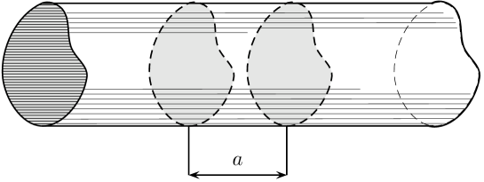
Figure 1: Two plates inside an infinite cylinder

To calculate the force on each of the two plates inside a cylinder with the cross section $M$ one can perform the following gedanken experiment that was frequently used to calculate the Casimir force between two infinite parallel perfectly conducting plates. Imagine that $4$ parallel plates are inserted inside an infinite cylinder and then $2$ exterior plates are moved to spatial infinity. This situation is exactly equivalent to $3$ perfectly conducting cavities touching each other. From the energy of this system one has to subtract the Casimir energy of an infinite cylinder without plates inside it, only then do we obtain the energy of interaction between the interior parallel plates, the one that can be measured in the experiment. Doing so we obtain the attractive force on each interior plate inside the cylinder:

$$F(a) =-\frac{\partial\mathcal{E}(a)}{\partial a},$$ (25)

$$\mathcal{E}(a) =\sum_{\omega_{wave}}\frac{1}{2}\ln(1-\exp(-2a\,\omega_{wave})),$$ (26)

the sum here is over all $TE$ and $TM$ eigenfrequencies $\omega_{wave}$ for a cylinder with the cross section $M$ and an infinite length.

In fact, the final results for this geometry should coincide with the results for the three plates’ piston geometry when one of the three piston plates (the exterior plate) is moved to infinity. Also one can immediately obtain the result for three plates’ system inside a cylinder, which is exactly the piston geometry, employing the same arguments and renormalization scheme. In the three plates’ system the force on the interior plate is equal to the sum of the forces acting on this plate from the two exterior plates, i.e. the piston geometry can be effectively considered as $2$ two plates’ systems. It should be emphasized that these assertions are valid for perfect boundary conditions.

By making use of an identity [15]

$$\frac{1}{2}\int_{-\infty}^{+\infty}\frac{dp}{2\pi}\ln\bigl{(}1-\exp(-2a\sqrt{\lambda^{2}+p^{2}})\bigr{)}=-\frac{\lambda}{2\pi}\sum_{l=1}^{+\infty}\frac{K_{1}(2l\lambda\,a)}{l}$$ (27)

one can rewrite (26) in the form:

$$\mathcal{E}(a)=-\frac{1}{2\pi}\sum_{l=1}^{+\infty}\biggl{(}\sum_{\lambda_{kD}}\frac{\lambda_{kD}K_{1}(2l\lambda_{kD}a)}{l}+\sum_{\lambda_{iN}}\frac{\lambda_{iN}K_{1}(2l\lambda_{iN}a)}{l}\biggr{)}.$$ (28)

The results (26) , (28) are our main zero temperature results. Our results are exact for an arbitrary curved geometry of a cylinder. This fact may be important for the experimental check of the Casimir effect in piston related geometries with curved boundaries. One can choose an arbitrary curved plate geometry $M$, for this geometry the eigenvalues of the two dimensional Dirichlet and Neumann problems $\lambda_{kD}$, $\lambda_{iN}$ can be found numerically. After that the exact expressions (26), (28) can be used to obtain the Casimir force on a plate. In fact, similar in the form mathematical results can be obtained in the case of a one dimensional massive scalar field theory on a manifold with boundary, however, in our case an infinite number of ”masses” $\lambda_{kD}$, $\lambda_{iN}$ appear in the theory due to existence of the cylinder cross section.

For convenience of the reader we write explicitly two special cases: rectangular and circular cylinders. For a rectangular cylinder with the sides $b$ and $c$ the exact Casimir energy of two plates inside it can be written as:

$$\mathcal{E}_{rect}(a)=-\sum_{l=1}^{+\infty}\sum_{m,n=-\infty}^{+\infty\>\prime}\frac{\sqrt{m^{2}/b^{2}+n^{2}/c^{2}}}{4l}\>\>K_{1}(2l\pi a\sqrt{m^{2}/b^{2}+n^{2}/c^{2}}).$$ (29)

The prime means that the term $m=n=0$ is omitted in the sum.

For a circular cylinder the eigenvalues of the two dimensional Laplace operator $\lambda_{kD},\lambda_{iN}$ are determined by the roots of Bessel functions and derivatives of Bessel functions. The exact Casimir energy of two circular plates of the radius $b$ separated by a distance $a$ inside an infinite circular cylinder of the radius $b$ is given by:

$$\mathcal{E}_{circ}(a)=-\sum_{l=1}^{+\infty}\sum_{\nu=0}^{+\infty}\sum_{j}\frac{1}{2\pi b}\frac{\mu_{D\nu j}K_{1}(2l\mu_{D\nu j}a/b)+\mu_{N\nu j}K_{1}(2l\mu_{N\nu j}a/b)}{l},$$ (30)

$$J_{\nu}(\mu_{D\nu j})=0,\>\>\>\>J_{\nu}^{{}^{\prime}}(\mu_{N\nu j})=0.$$

The sum is over positive $\mu_{D\nu j}$ and $\mu_{N\nu j}$.

The leading asymptotic behaviour of $\mathcal{E}(a)$ for long distances $\lambda_{1D}a\gg 1$, $\lambda_{1N}a\gg 1$ is determined by the lowest positive eigenvalues of the two dimensional Dirichlet and Neumann problems $\lambda_{1D},\lambda_{1N}$:

$$\mathcal{E}(a)|_{\lambda_{1D}a\gg 1,\>\lambda_{1N}a\gg 1}\sim-\frac{1}{4\sqrt{\pi a}}\Bigl{(}\sqrt{\lambda_{1D}}e^{-2\lambda_{1D}a}+\sqrt{\lambda_{1N}}e^{-2\lambda_{1N}a}\Bigr{)},$$ (31)

so the Casimir force between the two plates in a cylinder is exponentially small for long distances. This important property of the solution is due to the gap in the frequency spectrum or, in other words, it is due to the finite size of the cross section of the cylinder.

3 Finite temperature results

To get the free energy $\mathcal{F}(a,\beta)$ for bosons at nonzero temperatures ($T=1/\beta$) one has to make the substitutions:

$$p \to p_{m}=\frac{2\pi m}{\beta},$$ (32)

$$\int_{-\infty}^{+\infty}\frac{dp}{2\pi} \to\frac{1}{\beta}\sum_{m=-\infty}^{+\infty}.$$ (33)

Thus the free energy describing the interaction of the two parallel perfectly conducting plates inside an infinite perfectly conducting cylinder of an arbitrary cross section has the form:

$$\mathcal{F}(a,\beta)=$$

$$=\frac{1}{\beta}\sum_{\lambda_{kD}}\sum_{m=-\infty}^{+\infty}\>\frac{1}{2}\ln\Bigl{(}1-\exp\bigl{(}-2a\sqrt{\lambda_{kD}^{2}+p_{m}^{2}}\bigr{)}\Bigr{)}+$$

$$+\frac{1}{\beta}\sum_{\lambda_{iN}}\sum_{m=-\infty}^{+\infty}\>\frac{1}{2}\ln\Bigl{(}1-\exp\bigl{(}-2a\sqrt{\lambda_{iN}^{2}+p_{m}^{2}}\bigr{)}\Bigr{)}.$$ (34)

This is our central finite temperature result. Note that $\lambda_{iN}\neq 0$. For rectangular and circular cylinders one can substitute the explicitly known $\lambda_{kD}$, $\lambda_{iN}$ to (34) in analogy to (29) and (30).

The attractive force between the plates inside an infinite cylinder of the same cross section at nonzero temperatures is given by:

$$F(a,\beta) =-\frac{\partial\mathcal{F}(a,\beta)}{\partial a}=-\frac{1}{\beta}\sum_{\omega_{TD}}\frac{\omega_{TD}}{\exp(2a\omega_{TD})-1}$$

$$-\frac{1}{\beta}\sum_{\omega_{TN}}\frac{\omega_{TN}}{\exp(2a\omega_{TN})-1}.$$ (35)

Here $\omega_{TD}=\sqrt{p_{m}^{2}+\lambda^{2}_{kD}}$ and $\omega_{TN}=\sqrt{p_{m}^{2}+\lambda^{2}_{iN}}$.

In the long distance limit $a\gg\beta/(4\pi)$ one has to keep only $m=0$ term in $(\ref{r21})$. Thus the free energy of the plates inside a cylinder in the high temperature limit is equal to:

$$\mathcal{F}(a,\beta)|_{a\gg\beta/(4\pi)}=\frac{1}{2\beta}\sum_{\lambda_{kD}}\>\ln\Bigl{(}1-\exp(-2a\lambda_{kD})\Bigr{)}+\\ +\frac{1}{2\beta}\sum_{\lambda_{iN}}\>\ln\Bigl{(}1-\exp(-2a\lambda_{iN})\Bigr{)}.$$ (36)

One can check that the limit $\lambda_{1D}a\ll 1$, $\lambda_{1N}a\ll 1$ in (36) immediately yields the known high temperature result for two parallel perfectly conducting plates separated by a distance $a$ (see eq.(51) for details).

If the conditions $\lambda_{1D}a\gg 1$, $\lambda_{1N}a\gg 1$ are satisfied in addition to the condition $a\gg\beta/(4\pi)$ then the leading asymptotic behaviour of the free energy can be expressed via the lowest positive eigenvalues of the two dimensional Dirichlet and Neumann problems $\lambda_{1D}$ and $\lambda_{1N}$ as follows:

$$\mathcal{F}(a,\beta)|_{a\gg\beta/(4\pi),\>\lambda_{1D}a\gg 1,\>\lambda_{1N}a\gg 1}\sim-\frac{1}{2\beta}\bigl{(}e^{-2a\lambda_{1D}}+e^{-2a\lambda_{1N}}\bigr{)},$$ (37)

so the force between the two plates in a cylinder is exponentially small for large enough distances between them at finite temperatures as well.

4 Free energy: short distance behaviour

It is convenient to apply the technique of the heat kernel and zeta function to obtain the short distance behaviour of the free energy (34). It can be done by noting that if the heat kernel expansion

$$\sum_{\lambda_{i}}e^{-t\lambda_{i}^{2}}\underset{t\to 0}{\sim}\sum_{k=0}^{+\infty}t^{\frac{-d+k}{2}}c_{k}$$ (38)

exists ($d$ is a dimension of the Riemannian manifold) then one can write the expansion

$$\sum_{\lambda_{i}}e^{-\sqrt{t}\lambda_{i}}\underset{t\to 0}{\sim}\sum_{k=0}^{d-1}\frac{2\;\Gamma(d-k)}{\Gamma((d-k)/2)}\;\;t^{\frac{-d+k}{2}}c_{k}$$ (39)

by making use of the analytical structure of the zeta function.

The proof can be done as follows. Zeta function can be written in two different forms:

$$\zeta(s) =\sum_{\lambda_{i}}\frac{1}{\Gamma(s/2)}\int_{0}^{+\infty}dt\,t^{\frac{s}{2}-1}\exp(-t\lambda_{i}^{2}),$$ (40)

$$\zeta(s) =\sum_{\lambda_{i}}\frac{1}{2\Gamma(s)}\int_{0}^{+\infty}dt\,t^{\frac{s}{2}-1}\exp(-\sqrt{t}\lambda_{i}).$$ (41)

It is well known that residues at the poles of the zeta function are related to the coefficients $c_{k}$ of the heat kernel expansion (38):

$$c_{k}=\frac{1}{2}\>{\rm Res}_{s=d-k}\bigl{(}\zeta(s)\Gamma(s/2)\bigr{)},$$ (42)

which follows from (40) and (38). The expansion (39) now follows from (41) and (42).

The free energy (34) can be rewritten as follows:

$$\mathcal{F}(a,\beta)=\sum_{\lambda_{rD}^{(3)}}\frac{1}{\beta}\ln\Bigl{(}1-\exp(-2a\lambda_{rD}^{(3)})\Bigr{)}+\sum_{\lambda_{kD}}\frac{1}{2\beta}\ln\Bigl{(}1-\exp(-2a\lambda_{kD})\Bigr{)}+\\ +\sum_{\lambda_{sN}^{(3)}}\frac{1}{\beta}\ln\Bigl{(}1-\exp(-2a\lambda_{sN}^{(3)})\Bigr{)}-\sum_{\lambda_{iN}}\frac{1}{2\beta}\ln\Bigl{(}1-\exp(-2a\lambda_{iN})\Bigr{)}-\\ -\sum_{\lambda_{lN}}\frac{1}{\beta}\ln\Bigl{(}1-\exp(-2a\lambda_{lN}^{(1)})\Bigr{)}$$ (43)

Here the eigenvalues $\lambda_{rD}^{(3)}$ satisfy the equation $\Delta^{(3)}p_{r}(x,y,z)=-\lambda_{rD}^{(3)2}p_{r}(x,y,z)$ and $p_{r}(x,y,z)$ satisfy Dirichlet boundary conditions at the boundary of the manifold $[0,\beta/2]\times M$, the eigenvalues $\lambda_{sN}^{(3)}$ satisfy the equation $\Delta^{(3)}p_{s}(x,y,z)=-\lambda_{sN}^{(3)2}p_{s}(x,y,z)$ and $p_{s}(x,y,z)$ satisfy Neumann boundary conditions at the boundary of the manifold $[0,\beta/2]\times M$, $M$ is an arbitrary cross section of the cylinder. Here we sum over all nonzero eigenvalues $\lambda_{sN}^{(3)}$.

The eigenvalues $\lambda_{lN}^{(1)}$ satisfy the one dimensional Laplace equation with Neumann boundary conditions at the boundary of the manifold $[0,\beta/2]$. They appear due to the condition $\lambda_{iN}\neq 0$ in equation (34) and our decision to sum over all nonzero $\lambda_{sN}^{(3)}$ in (43). Thus in the last line of (43) the eigenvalues $\lambda_{sN}^{(3)}$ corresponding to the eigenfunctions $p_{n}(x,y,z)=\cos(2\pi nz/\beta)$ (for which $\lambda_{iN}=0$) are effectively subtracted.

Our strategy is the following: one expands the logarithms in the formula (43) in series

$$\ln(1-\exp(-2a\lambda_{i}))=-\sum_{n=1}^{+\infty}\frac{\exp(-2an\lambda_{i})}{n},$$ (44)

applies the expansion (39) to each term in (44) for short distances $a$ and performs the sum over $n$ thus getting Riemann zeta function at integer positive values.

It is possible to obtain the coefficients of the heat kernel expansion for the operators $\Delta^{(3)}$ along the following lines. For the manifold $[0,\beta/2]\times M$ and Dirichlet boundary conditions one can write:

$$\exp(-t\Delta^{(3)})\underset{t\to 0}{\sim}\Biggl{(}\frac{\beta/2}{\sqrt{4\pi}}\>t^{-1/2}-\frac{1}{2}\Biggr{)}\\ \Biggl{(}\frac{S}{4\pi}t^{-1}-\frac{P}{4\sqrt{4\pi}}\>t^{-1/2}+\sum_{i}\frac{1}{24}\Bigl{(}\frac{\pi}{\alpha_{i}}-\frac{\alpha_{i}}{\pi}\Bigr{)}+\frac{1}{12\pi}\int_{\gamma_{j}}L_{aa}(\gamma_{j})dl\Biggr{)}$$ (45)

Here $S$ is an area and $P$ is a perimeter of the cross section $M$, $\alpha_{i}$ is the interior angle of each sharp corner at the boundary $\partial M$ and $L_{aa}(\gamma_{j})$ is the curvature of each boundary smooth section described by the curve $\gamma_{j}$.

Thus the important for our purpose Seeley coefficients for the operator $\Delta^{(3)}$ with Dirichlet boundary conditions imposed at the boundary of the manifold $[0,\beta/2]\times M$ can be obtained from (45) as the coefficients at specific powers of $t$ in the expansion (38):

$$c_{0D}^{(3)} =\frac{\beta S}{2(4\pi)^{3/2}}$$ (46)

$$c_{1D}^{(3)} =-\frac{S}{8\pi}-\frac{\beta P}{32\pi}$$ (47)

$$c_{2D}^{(3)} =\frac{\beta}{4\sqrt{\pi}}\Biggl{(}\sum_{i}\frac{1}{24}\Bigl{(}\frac{\pi}{\alpha_{i}}-\frac{\alpha_{i}}{\pi}\Bigr{)}+\frac{1}{12\pi}\int_{\gamma_{j}}L_{aa}(\gamma_{j})dl\Biggr{)}+\frac{P}{16\sqrt{\pi}}$$ (48)

One can check by a direct calculation that $c_{0N}^{(3)}=c_{0D}^{(3)}$, $c_{1N}^{(3)}=-c_{1D}^{(3)}$, $c_{2N}^{(3)}=c_{2D}^{(3)}$ for manifold $[0,\beta/2]\times M$ with Neumann boundary conditions.

The other needed coefficients for manifold $M$ can also be read off from (45): $c_{1D}^{(2)}=-c_{1N}^{(2)}=-P/(8\sqrt{\pi})$, for manifold $[0,\beta/2]$: $c_{0N}^{(1)}=\beta/(4\sqrt{\pi})$.

For $a\ll\beta/(4\pi)$ and $\lambda_{1D}a\ll 1$, $\lambda_{1N}a\ll 1$ one obtains from (39) and (43) the leading terms for the free energy:

$$\mathcal{F}(a,\beta)|_{a\ll\beta/(4\pi),\>\lambda_{1D}a\ll 1,\>\lambda_{1N}a\ll 1}=-\frac{\zeta_{R}(4)}{8\pi^{2}}\frac{S}{a^{3}}-\frac{\zeta_{R}(2)}{4\pi a}(1-2\chi)+O(1),$$ (49)

where

$$\chi=\sum_{i}\frac{1}{24}\Bigl{(}\frac{\pi}{\alpha_{i}}-\frac{\alpha_{i}}{\pi}\Bigr{)}+\sum_{j}\frac{1}{12\pi}\int_{\gamma_{j}}L_{aa}(\gamma_{j})d\gamma_{j}.$$ (50)

The force calculated from (49) coincides with the zero temperature force $F_{C}$ in [3], (Eq.7). Thus we prove that in the finite temperature case the leading short distance terms are the same as in the zero temperature case.

In the limit $\lambda_{1D}a\ll 1$, $\lambda_{1N}a\ll 1$ one immediately obtains from (36) the high temperature result for two parallel perfectly conducting plates separated by a distance $a$. One expands logarithms in series and uses (39) and $c_{0D}=c_{0N}=S/(4\pi)$ in two dimensions ($d=2$) to obtain:

$$\mathcal{F}(a,\beta)|_{a\gg\beta/(4\pi),\>\lambda_{1D}a\ll 1,\>\lambda_{1N}a\ll 1}=\\ =-\sum_{\lambda_{kD}}\frac{1}{2\beta}\sum_{n=1}^{+\infty}\frac{\exp(-2an\lambda_{kD})}{n}\Bigl{|}_{a\to 0}-\sum_{\lambda_{iN}}\frac{1}{2\beta}\sum_{n=1}^{+\infty}\frac{\exp(-2an\lambda_{iN})}{n}\Bigr{|}_{a\to 0}=\\ =\sum_{n=1}^{+\infty}-\frac{1}{2\beta}\frac{1}{n}\frac{1}{(2an)^{2}}2(c_{0D}+c_{0N})=-\frac{\zeta_{R}(3)}{\beta a^{2}}\frac{S}{8\pi},$$ (51)

which is a well known result [16, 17, 18].

References

• [1] H.B.G.Casimir, K.Ned.Akad.Wet.Proc.51, 793 (1948).
• [2] R.M.Cavalcanti, Phys.Rev.D 72, 065015 (2004) [arXiv: quant-ph/0310184].
• [3] M. P. Hertzberg, R. L. Jaffe, M. Kardar and A. Scardicchio, Phys. Rev. Lett. 95, 250402 (2005) [arXiv: quant-ph/0509071].
• [4] G.Barton, Phys.Rev.D 73, 065018 (2006).
• [5] S.A.Fulling and J.H.Wilson, Repulsive Casimir Pistons [arXiv: quant-ph/0608122].
• [6] A.Edery, Casimir piston for massless scalar fields in three dimensions [arXiv: hep-th/0610173].
• [7] Xiang-hua Zhai, Xin-zhou Li, Casimir pistons with hybrid boundary conditions [arXiv: hep-th/0612155].
• [8] E.M.Santangelo, Theor.Math.Phys. 131, 527 (2002); Teor.Mat.Fiz.131, 98 (2002) [arXiv: hep-th/0104025].
• [9] E. Elizalde, S. D. Odintsov, A. Romeo, A.Bytsenko and S. Zerbini, ”Zeta regularization with applications”, World Sci., Singapore, 1994.
• [10] D.Β V.Β Vassilevich, Phys.Rept. 388, 279 (2003) [arXiv:hep-th/0306138].
• [11] P.Β B.Β Gilkey, ”Invariance theory, the heat equation, and the Atiyah-Singer index theorem”, CRC Press, 1994.
• [12] V.N.Marachevsky, One loop boundary effects: techniques and applications [arXiv: hep-th/0512221].
• [13] W.Lukosz, Physica(Amsterdam) 56, 109 (1971).
• [14] M.Bordag, U.Mohideen, V.M.Mostepanenko, Phys.Rept. 353, 1 (2001) [arXiv: quant-ph/0106045].
• [15] V.V.Nesterenko and I.G.Pirozhenko, J.Math.Phys.38, 6265 (1997) [arXiv: hep-th/9703097].
• [16] I.Brevik, S.A.Ellingsen and K.A.Milton, New J. Phys. 8, 236 (2006) [arXiv: quant-ph/0605005].
• [17] F.Sauer, PhD Thesis Gottingen, 1962.
• [18] E.M.Lifshitz, Zh.Eksp.Teor.Fiz. 29, 94 (1956) [ Soviet Phys. JETP 2, 73]; I.D.Dzyaloshinskii, E.M.Lifshitz and L.P.Pitaevskii, Usp.Fiz.Nauk 73, 381 (1961) [ Soviet Phys.Usp.4, 153].