The conformal anomaly of k-strings

Abstract:

Simple scaling properties of correlation functions of a confining gauge theory in d-dimensions lead to the conclusion that k-string dynamics is described, in the infrared limit, by a two-dimensional conformal field theory with conformal anomaly $c=(d-2)\sigma_{k}/\sigma$, where $\sigma_{k}$ is the k-string tension and $\sigma$ that of the fundamental representation. This result applies to any gauge theory with stable k-strings. We check it in a 3D $\Z_{4}$ gauge model at finite temperature, where a string effect directly related to $c$ can be clearly identified.

1 Introduction

One of the simplest and most general consequences of the effective string description of the quark confinement [1, 2, 3] is the presence of measurable effects on physical observables of the gauge theory, produced by the quantum fluctuations of that string [4, 5]. The most widely known is the Lüscher correction to the interquark confining potential $V$ at large distance $r$

$$V(r)=\sigma\,r+2\,\mu-(d-2)\frac{\pi}{24r}+O(1/r^{2})\,,$$ (1)

where $\sigma$ is the string tension and $\mu$ a self-energy term. The attractive, Coulomb-like correction is universal in the sense that it is the same for whatever confining gauge theory and depends only on the $d-2$ transverse oscillation modes of the string.

A similar universal effect has been found in the low temperature behaviour of the string tension [6]

$$\sigma(T)=\sigma-(d-2)\frac{\pi}{6}T^{2}+O(T^{4})\,.$$ (2)

Both effects may be rephrased by saying that the infrared limit of the effective string is described by a two-dimensional conformal field theory (CFT) with conformal anomaly $c=d-2$. In this language, the (generalised) Lüscher term $-\frac{c\,\pi}{24\,r}$ is the zero-point energy of a 2D system of size $r$ with Dirichlet boundary conditions, while the $-\frac{c\,\pi}{6}T^{2}$ term is the zero-point energy density in a cylinder (i.e. the string world-sheet of the Polyakov correlator) of period $L=1/T$ [7].

In this paper we propose a method to extend these results to a more general class of confining objects of $\mathop{\rm SU}(N)$ gauge theories, the k-strings, describing the infrared behaviour of the flux tube joining sources in representations with $N-$ality $k$. There are of course infinitely many irreducible representations corresponding to the same value of $k$. No matter what representation $\mathscr{R}$ is chosen, the stable string tension $\sigma_{k}$ depends only on the $N-$ality $k$ of $\mathscr{R}$, i.e. on the number (modulo $N$) of copies of the fundamental representation needed to build $\mathscr{R}$ by tensor product, since the sources may be screened by gluons. As a consequence, at sufficiently large distances, the heavier strings find it energetically favourable to decay into the string of smallest string tension, called k-string.

The spectrum of k-string tensions has been extensively studied in recent years, in the continuum [8]–[16] as well as on the lattice [17]–[24]. So far, in numerical analyses one typically measured the temperature-dependent k-string tensions $\sigma_{k}(T)$ through the Polyakov correlators and then extrapolated to $T=0$ using (2), hence assuming a free bosonic string behaviour.

Recently this assumption has been questioned by a numerical experiment. It showed that in a 3D $\Z_{4}$ gauge theory, though the 1-string fitted perfectly the free string formulae with a much higher precision than in the $\mathop{\rm SU}(N)$ case, the 2-string failed to meet free string expectations [25]. One could object that there is no compelling reason for a 2-string of a $\Z_{4}$ gauge system to behave like a 2-string of $\mathop{\rm SU}(N)$ gauge system; a k-string can be seen as a bound state of $k$ 1-strings and the binding force would presumably depend on the specific properties of the gauge system.

On the other hand, from a theoretical point of view there are good reasons to expect values of $c$ larger than $d-2$. In fact the conformal anomaly can be thought of as counting the number of degrees of freedom of the k-string. Therefore the relevant degrees of freedom are not only the transverse displacements but also the splitting of the k-string into its constituent strings. If the mutual interactions where negligible, each constituent string could vibrate independently so we had $c=k\,(d-2)$. Thus we expect that $c$ can vary in the range

$$d-2\leq\,c\,\leq k\,(d-2)\,.$$ (3)

An unexpected insight into the actual value of $c$ comes when considering the infrared properties of the N-point Polyakov correlators related to the baryon vertex of $\mathop{\rm SU}(N)$

$$\langle\,P_{f}(\vec{r}_{1})\,P_{f}(\vec{r}_{2})\dots P_{f}(\vec{r}_{N})\,\rangle_{T}\,,$$ (4)

where $P_{f}(\vec{r}_{i})$ is the Polyakov line in the fundamental representation identified by $d-1$ spatial coordinates $\vec{r}_{i}$ and directed along the periodic temporal direction of size $L=1/T$. If all the distances $|\vec{r}_{i}-\vec{r}_{j}|$ are much larger than any other relevant scale, this correlator is expected to obey a simple scaling property. When combining this fact with the circumstance that, depending on the positions $\vec{r}_{i}$ of the sources, some strings of the baryon vertex may coalesce into k-strings [26, 13], one obtains the geometric constraint

$$\sigma_{k}(T)=\sigma_{k}-(d-2)\frac{\pi\,\sigma_{k}}{6\,\sigma}\,T^{2}+O(T^{3})\,,$$ (5)

which is the main result of this paper. We check this formula in a 3D $\Z_{4}$ gauge model where, thanks to duality, very efficient simulation techniques are available, yielding high precision results which give fairly convincing evidence for the scaling law (5).

The contents of this paper are as follows. In the next Section we expose in detail the above-mentioned scaling argument, while in the following Section we describe a lattice calculation on a three-dimensional $\Z_{4}$ gauge theory where combining duality transformation with highly efficient simulation techniques it is possible to confirm that the stable 2-string matches nicely Eq.(5). We finish with a discussion of our results and some of their implications.

2 Scaling form of the Polyakov correlators

The main role of the string picture of confinement is to fix the functional form of the vacuum expectation value of gauge invariant operators in the infrared limit. It predicts two different asymptotic behaviours of the correlation function of a pair of Polyakov loops $\langle P_{f}(\vec{r}_{1})\,P^{\dagger}_{f}(\vec{r}_{2}\rangle_{T}$, when both $r\equiv|\vec{r}_{1}-\vec{r}_{1}|$ and $L\equiv 1/T$ are large, depending on the value of the ratio $2r/L$. Using (1) and (2) we can write

$$-\frac{1}{L}\log\langle P_{f}(\vec{r}_{1})\,P^{\dagger}_{f}(\vec{r}_{2})\rangle_{T}=V(r)+O(e^{-\pi\,L/r})~{},~{}~{}2\,r<\,L\,,$$ (6)

$$-\frac{1}{L}\log\langle P_{f}(\vec{r}_{1})\,P^{\dagger}_{f}(\vec{r}_{2})\rangle_{T}=\sigma(T)\,r+2\mu+\frac{1}{2L}\log{\frac{2r}{L}}+O(e^{-4\pi r/L})~{},~{}~{}2\,r>\,L\,,$$ (7)

where $V(r)$ and $\sigma(T)$ are given by (1) and (2). There are strong indications that the $r^{-3}$ and $T^{3}$ terms are zero and the $r^{-4}$ and $T^{4}$ are universal (see for instance the discussion in [27] and references quoted therein). For our purposes we need only the first universal term, which is directly related to the central charge of the CFT describing the IR limit of the underlying confining string. In this approximation the Polyakov loop correlation functions should decay at large $r$ while keeping constant $T$ as

$$\langle P_{f}(\vec{r}_{1})\,P^{\dagger}_{f}(\vec{r}_{2})\rangle_{T}\stackrel{{\scriptstyle\sim}}{{\propto}}\exp\left[-\sigma(T)\,r\,L-2\mu\,L\right]\,.$$ (8)

Similar expansions are expected to be valid also for Polyakov correlators describing more specific features of $\mathop{\rm SU}(N)$ gauge theory, like those involving baryonic vertices.

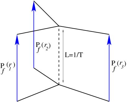
Figure 1: The three-bladed world-sheet of a static SU(3) baryon.

A baryon vertex is a gauge-invariant coupling of $N$ multiplets in the fundamental representation $f$ which gives rise to configurations of finite energy, or baryonic potential, with $N$ external sources. At finite temperature $T$ these sources are the Polyakov lines $P_{f}(\vec{r}_{i})$. Assume for a moment $N=3$. When the mutual distances $|\vec{r}_{i}-\vec{r}_{j}|$ $(i,j=1,2,3)$ are all large, three confining strings of chromo-electric flux form, which, starting from the three sources, meet a common junction; their world-sheet forms a three-bladed surface with a common intersection [28, 29] (see Fig.1).

The total area $\mathbb{A}$ of this world-sheet is $L\,\ell(\vec{r}_{1},\vec{r}_{2},\vec{r}_{3})$ where $\ell$ is the total length of the string. The stable configuration (hence the position of the common junction) is the one minimising $\mathbb{A}$. The balance of tensions implies angles of $\frac{2\pi}{3}$ between the blades.

The complete functional form of the 3-point correlator is substantially unknown. Nonetheless, the static baryon potential, defined as

$$V=-\lim_{T\to\infty}T\,\log\langle\,P_{f}(\vec{r}_{1})\,P_{f}(\vec{r}_{2})\,P_{f}(\vec{r}_{3})\,\rangle_{T}\,,$$ (9)

has a simple form in the IR limit:

$$V=\sigma\,\ell(\vec{r}_{1},\vec{r}_{2},\vec{r}_{3})+3\mu+\dots$$ (10)

The universal $1/r$ corrections have been calculated in [30].

In the IR limit at finite temperature, i.e. $|\vec{r}_{i}-\vec{r}_{j}|\gg L~{}\forall i\not=j$, we assume, in analogy with (8),

$$\langle\,P_{f}(\vec{r}_{1})\,P_{f}(\vec{r}_{2})\dots P_{f}(\vec{r}_{N})\,\rangle_{T}=e^{-F_{N}}\sim\exp\left[-\sigma(T)\,L\,\ell(\vec{r}_{1},\vec{r}_{2},\dots,\vec{r}_{N})-N\mu\,L\right]\,,$$ (11)

or, more explicitly,

$$F_{N}(\ell,L)\sim\sigma\,L\ell-(d-2)\frac{\pi\,\ell}{6\,L}+N\mu\,L~{},\,~{}(|\vec{r}_{i}-\vec{r}_{j}|\gg L~{}\forall i\not=j)\,,$$ (12)

where the coefficient of the $\ell/L$ term specifies that in this IR limit the behaviour of the baryon flux distribution is described by a CFT with conformal anomaly $d-2$ on the string world-sheet singled out by the position of the external sources.

The above considerations are completely standard and nothing new happens so far.

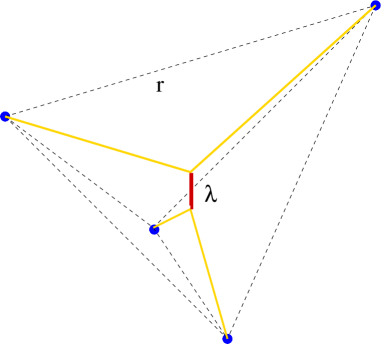
Figure 2: Confining string configuration of a SU(4) static baryon. The thick line is a 2-string.

The surprise comes when considering the latter expression in the case $N>3$. Notice that, depending on the positions $\vec{r}_{i}$ of the sources, some fundamental strings of the baryon vertex may coalesce into k-strings [26, 13]. As a consequence, the shape of the world-sheet changes in order to balance the string tensions and $\ell$ becomes a weighted sum, where a k-string of length $\lambda$ contributes with a term $\lambda\,\frac{\sigma_{k}(T)}{\sigma(T)}\,$, where $\sigma(T)$ is given by (2), while

$$\sigma_{k}(T)=\sigma_{k}-c_{k}\,\frac{\pi}{6}T^{2}+O(T^{3})\,,$$ (13)

where $c_{k}$ is the conformal anomaly of the k-string. When the string is in the fundamental representation the $T^{3}$ term (2) is missing [31, 32, 33], however we cannot exclude it in the k-string with $k>1$. The string tension ratio is

$$\frac{\sigma_{k}(T)}{\sigma(T)}=\frac{\sigma_{k}}{\sigma}+\frac{\sigma_{k}}{\sigma}\left(\frac{d-2}{\sigma}-\frac{c_{k}}{\sigma_{k}}\right)\frac{\pi}{6}T^{2}+O(T^{3})\,;$$ (14)

if the coefficient of the $T^{2}$ term does not vanish the asymptotic functional form (12) of the free energy gets modified.

As a simple, illustrative example, let us consider the chromo-electric flux distribution of a 4D $SU(4)$ gauge system generated by four external quarks placed at the vertices of a regular tetrahedron (see Fig. 2). Preparing the external sources in a symmetric configuration does not necessarily imply that the distribution of the gauge flux preserves the tetrahedral symmetry. In fact, the formation of a 2-string breaks this symmetry (see Fig.2). The actual symmetry breaking or restoration depends on the cost in free energy of the configuration, of course. It is easy to show that, when $\frac{\sigma_{2}}{\sigma}<\frac{2}{\sqrt{3}}$, the tetrahedral symmetry is spontaneously broken [13] and the length $\lambda$ of the 2-string, which is a function of the ratio $\sigma_{2}/\sigma$, is given by

$$\lambda=\frac{r}{\sqrt{2}}-\frac{r\,\sigma_{2}}{\sqrt{4\,\sigma^{2}-\sigma_{2}^{2}}}\,,$$ (15)

where $r$ is the edge length. The free energy $F_{4}$ of the four-quark system is

$$F_{4}=\sigma(T)\,L\,\ell(T)+4\mu L=\sigma(T)\,L\,\left(2\,r\sqrt{1-\left(\frac{\sigma_{2}(T)}{2\sigma(T)}\right)^{2}}+\frac{r}{\sqrt{2}}\,\frac{\sigma_{2}(T)}{\sigma(T)}\right)+4\mu\,L\,.$$ (16)

Now the total length $\ell$ of the string may depend on $T$ through the ratio $\sigma_{2}(T)/\sigma(T)$. Expanding in $T=1/L$ as in (14) we get

$$F_{4}=\sigma\,L\,\ell(0)-\frac{\pi}{6}\left[(d-2)\frac{\ell(0)}{L}-{\sigma_{2}}\left(\frac{d-2}{\sigma}-\frac{c_{2}}{\sigma_{2}}\right)\frac{\lambda}{L}\right]+4\mu\,L+O(1/L^{2})\,.$$ (17)

Clearly the term proportional to $\lambda$ violates the expected asymptotic form of the free energy (12), unless $c_{2}=(d-2)\,\sigma_{2}/\sigma\,$.

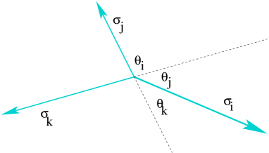
Figure 3: The balance of the string tensions.

More generally, the baryonic free energy keeps the expected asymptotic form (12) only if the world-sheet shape does not change while varying $T$. Now in a generic string configuration contributing to $\mathop{\rm SU}(N)$ baryon potential, the angles at a junction of three arbitrary k-strings are given by (see Fig.3)

$$\cos\theta_{i}=\frac{\sigma_{j}(T)^{2}+\sigma_{k}(T)^{2}-\sigma_{i}(T)^{2}}{2\,\sigma_{j}(T)\,\sigma_{k}(T)}$$ (18)

and others obtained by cyclic permutations of the indices $i,j,k$. As a consequence, these angles are kept fixed only if all the string tension ratios are constant up to $T^{3}$ terms, i.e. only if

$$\frac{c_{i}}{\sigma_{i}}=\frac{c_{j}}{\sigma_{j}}=\frac{c_{k}}{\sigma_{k}}=\frac{(d-2)}{\sigma}$$ (19)

which leads directly to

$$\sigma_{k}(T)=\sigma_{k}-(d-2)\frac{\pi\,\sigma_{k}}{6\,\sigma}\,T^{2}+O(T^{3})$$ (20)

as anticipated in the Introduction.

3 The 3D $\Z_{4}$ gauge model and its dual

The above general argument on the finite temperature corrections of the k-string tensions suggests a different behaviour with respect to the usual assumption that these corrections are those produced by a free bosonic string. Since the comparison with theoretical predictions of k-string tensions is sensitive to this behaviour, it is important to check its validity.

In this Section we address such a question with a lattice calculation in a 3D $\Z_{4}$ gauge theory which is perhaps the simplest gauge system where there is a stable 2-string.

We work on a periodic cubic lattice $L\times L\times L_{\tau}$. The degrees of freedom are the fourth roots of the identity $\zeta_{l}$ $~{}(\zeta^{4}=1)$, defined on the links $l$ of the lattice. The partition function is

$$Z(\beta_{f},\beta_{ff})=\prod_{l}\sum_{\zeta_{l}=\pm 1,\pm i}e^{\sum_{p}(\beta_{f}{\cal U}_{p}+\beta_{ff}{\cal U}^{2}_{p}/2+c.c.)}\,,$$ (21)

where the sum is extended to all plaquettes $p$ of the lattice and ${\cal U}_{p}=\prod_{l\in p}\zeta_{l}$; $\beta_{f}$ and $\beta_{ff}$ are two coupling constants. When they vary in a suitable range the system belongs to a confining phase. In analogy with the $\mathop{\rm SU}(N)$ case we say that ${\cal U}_{p}$ is in the fundamental ($f$) representation while ${\cal U}_{p}^{2}$ lies in the double-fundamental ($ff$) representation. From a computational point of view it is convenient to recast $Z$ as the partition function of two coupled $\Z_{2}$ gauge systems

$$Z(\beta_{f},\beta_{ff})=\prod_{l}\sum_{\{U_{l}=\pm 1,V_{l}=\pm 1\}}e^{\sum_{p}\beta_{f}(U_{p}+V_{p})+\beta_{ff}U_{p}V_{p}}\,,~{}\left(U_{p}=\prod_{l\in p}U_{l}\,,V_{p}=\prod_{l\in p}V_{l}\right)\,.$$ (22)

The external sources generating the 1-string and the 2-string are given respectively by the two products

$$P_{f}(\vec{r})\equiv\prod_{l\in\gamma_{\vec{r}}}U_{l}~{}{\rm or}~{}\prod_{l\in\gamma_{\vec{r}}}V_{l}~{};~{}~{}P_{ff}(\vec{r})\equiv\prod_{l\in\gamma_{\vec{r}}}U_{l}\,V_{l}\,,$$ (23)

where $\gamma_{\vec{r}}$ is a closed path in the lattice which winds once around the temporal direction $L_{\tau}$ and passes through $\vec{r}$.

This model, as any three-dimensional abelian gauge system, admits a spin model as its dual. We have recently shown [34] that this $\Z_{4}$ gauge model is dual to a spin model with global $\Z_{4}$ symmetry which can be written as a symmetric Ashkin-Teller (AT) model, i.e. two coupled Ising models defined by the two-parameter action

$$S_{AT}=-\sum_{\langle xy\rangle}\left[\beta(\sigma_{x}\sigma_{y}+\tau_{x}\tau_{y})+\alpha(\sigma_{x}\sigma_{y}\tau_{x}\tau_{y})\right]\,,$$ (24)

where $\sigma_{x}$ and $\tau_{x}$ are Ising variables ($\sigma,\tau=\pm 1$) associated to the site $x$ and the sum is over all the links $\langle xy\rangle$ of the dual cubic lattice. The two couplings $\alpha$ and $\beta$ are related to the gauge couplings $\beta_{f}$ and $\beta_{ff}$ by [34]

$$\alpha = \frac{1}{4}\log\left(\frac{(\coth\beta_{f}+\tanh\beta_{f}\tanh\beta_{ff})(\coth\beta_{f}+\tanh\beta_{f}\coth\beta_{ff})}{2+\tanh\beta_{ff}+\coth\beta_{ff}}\right)\,,$$ (25)

$$\beta = \frac{1}{4}\log\left(\frac{1+\tanh^{2}\beta_{f}\tanh\beta_{ff}}{\tanh^{2}\beta_{f}+\tanh\beta_{ff}}\right)\,.$$ (26)

The duality transformation maps any physical observable of the gauge theory into a corresponding observable of the spin model. In particular it is well known that the Wilson loops are related to suitable flips of the couplings of the spin model. We have found the identity

$$\langle\hskip 1.99997ptV_{P}\hskip 1.99997pt\rangle_{gauge}=\langle\hskip 1.99997pte^{-2(\beta+\alpha\tau_{x}\tau_{y})\sigma_{x}\sigma_{y}}\hskip 1.99997pt\rangle_{AT}$$ (27)

generalising the known dual identity of the Ising model. Similarly, flipping the signs of both spins $\sigma_{x}$ and $\tau_{x}$ we get the plaquette variable in the $k=2$ representation as $\langle\hskip 1.99997ptU_{P}V_{P}\hskip 1.99997pt\rangle$. Combining together a suitable set of plaquettes we may build up any Wilson loop or Polyakov-Polyakov correlator with $k=1$ or $k=2$.

3.1 Monte Carlo simulations

Our interest in writing this model in terms of Ising variables is twofold.

First we can easily apply for the simulation a very efficient non-local algorithm [35], basically similar to the standard Fortuin-Kasteleyn cluster method of Ising systems: each update step is composed by an update of the $\sigma$ variables using the current values of the $\tau$’s as a background (thus locally changing the coupling from $\beta$ to $\beta\pm\alpha$ according to the value of $\tau_{x}\tau_{y}$ on the link $\langle xy\rangle$), followed by an update of the $\tau$’s using the $\sigma$ values as background.

		$\alpha=0.05$	$\alpha=0.07$
		$\beta=0.2070$	$\beta=0.1975$
$\sigma\equiv\sigma_{f}$		0.02085(10)	0.0157(1)
$\sigma_{2}\equiv\sigma_{ff}$		0.0328(5)	0.0210(5)
$\sigma_{2}-\sigma$		0.01195(51)	0.0053(5)
	$N_{\tau}=9$	0.00864(6)	–
	$N_{\tau}=10$	0.00951(8)	0.003700(30)
	$N_{\tau}=11$	0.01010(10)	0.004220(35)
	$N_{\tau}=12$	0.01050(15)	0.004550(35)
$\Delta\,\sigma(T)$	$N_{\tau}=13$	0.01080(20)	0.004750(40)
	$N_{\tau}=14$	0.01100(25)	0.004910(40)
	$N_{\tau}=15$	–	0.005020(45)
	$N_{\tau}=16$	–	0.005110(50)
$\Delta\,\sigma(0)$		0.01271(2)	0.00591(1)

Table 1: String tension differences $\Delta\sigma(T)$ as resulting from fits to Eq.(30). $\Delta\,\sigma(0)$ is evaluated from a fit to Eq.(31) using $\Delta\sigma(T)$ data. All the quantities are expressed in lattice spacing units.

Secondly, by flipping a suitable set of couplings, we can insert any Wilson loop or Polyakov correlator directly in the Boltzmann factor, producing results with very high precision. If, for instance, we generate a sequence of Monte Carlo configurations where the $\sigma_{x}$ couplings of all the links crossing the cylindric surface bounded by the Polyakov lines $\gamma_{\vec{r}_{1}}$ and $\gamma_{\vec{r}_{2}}$ are flipped, then the average of whatever observable ${\cal Q}$ is actually the quantity

$$\frac{\langle\,{\cal Q}\,P_{f}(\vec{r}_{1})\,P^{\dagger}_{f}(\vec{r}_{2})\rangle_{T}}{\langle\,P_{f}(\vec{r}_{1})\,P^{\dagger}_{f}(\vec{r}_{2})\rangle_{T}}\,.$$ (28)

In our numerical experiment we choose ${\cal Q}=P_{f}(\vec{r}_{1})\,P^{\dagger}_{f}(\vec{r}_{2})$, therefore the corresponding averages yield directly, according to (23), the ratio

$$R(|\vec{r}_{1}-\vec{r}_{2}|,T)=\frac{\langle\,P_{ff}(\vec{r}_{1})\,P_{ff}(\vec{r}_{2})\rangle_{T}}{\langle\,P_{f}(\vec{r}_{1})\,P^{\dagger}_{f}(\vec{r}_{2})\rangle_{T}}\,.$$ (29)

We estimated this vacuum expectation value with a very powerful method, based on the linking properties of the FK clusters [36]: for each FK configuration generated by the above-mentioned algorithm one looks for paths in the clusters linked with the loops $\gamma_{\vec{r}_{1}}$ and $\gamma_{\vec{r}_{2}}$. If there is no path of this kind we put ${\cal Q}=1$, otherwise we set ${\cal Q}=0$. The algorithm we used to determine the linking properties is described in [37]. This method leads to an estimate of $R(|\vec{r}_{1}-\vec{r}_{2}|,T)$ with reduced variance with respect to the conventional numerical estimates.

3.2 Results

We performed our Monte Carlo simulations on the AT model, at two different points of the confining region, for which we measured previously the string tensions [25] (see Table 1) . We worked on a cubic periodic lattice of size $128\times 128\times N_{\tau}$ with $N_{\tau}$ chosen in such a way that temperature of our simulations ranged from $T/T_{c}\simeq 0.5$ to $T/T_{c}\simeq 0.8$ and we took the averages over $10^{6}$ configurations in each point.

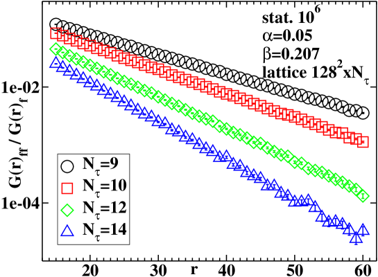
Figure 4: Plot of $G(r)_{ff}/G(r)_{f}$ on a log scale.

The large distance behaviour of the data is well described by a purely exponential behaviour (see Fig.4)

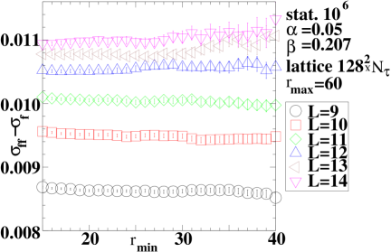
Figure 5: The fitted value of $\Delta\sigma$ to Eq.(30) as a function of the minimal distance $r_{min}$ considered for different values of $N_{\tau}$. The large plateaux show the stability of the fit.

$$G(r)_{ff}/G(r)_{f}=\frac{\langle\,P_{ff}(\vec{r}_{1})\,P_{ff}(\vec{r}_{2})\rangle_{T}}{\langle\,P_{f}(\vec{r}_{1})\,P^{\dagger}_{f}(\vec{r}_{2})\rangle_{T}}\propto e^{-\Delta\sigma\,r\,N_{\tau}}\,,$$ (30)

with $\Delta\,\sigma=\sigma_{ff}-\sigma_{f}$. Comparison with (7) shows that the logarithmic term, which is a potential source of systematic errors when neglected in Polyakov correlators, here is cancelled in the ratio. Since (30) is an asymptotic expression, valid in the IR limit, we fitted the data to the exponential by progressively discarding the short distance points and taking all the values in the range $r_{min}\leq r\leq r_{max}=60\,a$ with $r_{min}$ varying from 15 to 40 lattice spacings $a$. The resulting value of $\Delta\sigma$ turns out to be very stable, as Fig. 5 shows. The whole set of values of $\Delta\,\sigma(T)$ as functions of the inverse temperature $N_{\tau}=1/T$ are reported in Table 1.

According to Eq.(5), in the low temperature limit we expect the asymptotic behaviour

$$\Delta\,\sigma(T)=\Delta\,\sigma(0)\left(1-\frac{\pi}{6\,\sigma}T^{2}\right)+O(T^{3})\,.$$ (31)

Assuming for $\sigma$ the values estimated in [25], we used $\Delta\sigma(0)$ as the only fitting parameter. Neglecting one or two points too close to $T_{c}$ we got very good fits to (31) as shown in Figs. 6 and 7. The fitting parameter $\Delta\,\sigma(0)$ as well as the estimates of $\Delta\,\sigma(T)$ are reported in Table 1. Note that $\Delta\,\sigma(0)$ agrees with the difference of the previous estimates [25], also reported in Table 1, however the error is reduced by a factor of 25 (first set of data) and even of 50 (second set of data). The reason of this gain in precision is due to the fact that $\sigma_{2}$ was evaluated from a fit to (8), even taking in account the Next-to-Leading-Order terms, which was rather poor because the 2-string does not behave as a free bosonic string [25]. On the contrary our fits to (30) and (31) are very stable and the corresponding reduced $\chi^{2}/d.o.f$ are of the order of 1 or less.

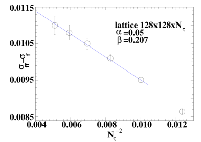
Figure 6: Values of $\Delta\sigma(T)$ from the first set of data of Table 1 versus $T^{2}=1/N^{2}_{\tau}$. The solid line is a one-parameter fit to Eq.(31).

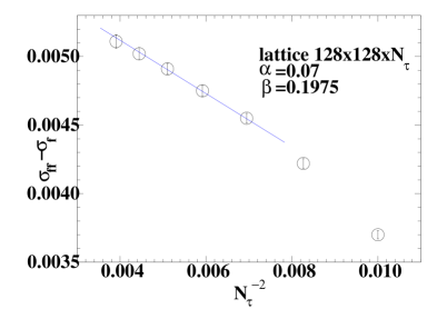
Figure 7: Same as Fig.6, but for the second set of data of Table 1.

4 Discussion

Our calculations in this paper were in two parts. In the first part we investigated the string nature of long flux tubes generated in an $\mathop{\rm SU}(N)$ gauge theory by external sources in representations with $N-$ality $k>1$. In a previous work [25] we were led to the conclusion that these k-strings are not adequately described by the free bosonic string picture. In this paper we argued that the central charge of the effective k-string theory is not simply $d-2$, like in the free bosonic string, but $c_{k}=(d-2)\frac{\sigma_{k}}{\sigma}$. This simple recipe was a straightforward consequence of demanding that the asymptotic functional form of Polyakov correlators associated to the baryon vertex should not change when varying the mutual positions of the Polyakov lines, the reason being that certain positions create k-strings inside the baryon vertex which modify the functional form of the correlator unless $\frac{\sigma_{k}(T)}{\sigma(T)}={\rm constant}+O(T^{3})$. This in turn fixes unambiguously the value of $c_{k}$. Although the geometric derivation is quite general and the resulting expression for $c_{k}$ is appealing for its simplicity, it would be very important to find some independent quantum argument in support of it.

The second part of the paper dealt with 2-strings in a 3D $\Z_{4}$ gauge model and in particular with the difference $\Delta\sigma(T)=\sigma_{2}(T)-\sigma(T)$ of the string tensions as a function of the temperature. Combining together three essential ingredients, namely the duality transformation, an efficient non-local cluster algorithm and finally a choice of flipped links which allows to directly measure the ratio of Polyakov correlators belonging to different representations, we obtained values for $\Delta\sigma(T)$ with unprecedented precision which nicely agree with our general formula (5). There is however much scope for improving these calculations: as Fig. 6 and 7 show, with little more effort it would be possible to evaluate also the corrections of order $T^{3}$ and $T^{4}$, that in the case of fundamental string are expected to be universal.

- [1] Y. Nambu, in Proc. Int. Conf. on Symmetries and Quark Models, Wayne State University 1969 (Gordon and Breach, 1970) p. 269.
- [2] Y. Nambu, Phys. Rev. D 10 (1974) 4262.
- [3] Y. Nambu, Phys. Lett. B 80 (1979) 372.
- [4] M. Lüscher, K. Symazik and P. Weisz, Nucl. Phys. B 173 (1980) 365.
- [5] M. Lüscher, Nucl. Phys. B 180 (1981) 317.
- [6] R.D. Pisarski and O. Alavarez, Phys. Rev. D 26 (1982) 3735.
- [7] H.W.J. Blöte, J.L. Cardy and M.O. Nightingale, Phys. Rev. Lett. 56 (1986) 343; I. Afflek, Phys. Rev. Lett. 56 (1986) 347.
- [8] M.R. Douglas and S.H. Shenker, Nucl. Phys. B 447 (1995) 271 [hep-th/9503163].
- [9] A. Hanany, M.J. Strassler and A. Zaffaroni, Nucl. Phys. B 513 (1998) 87 [hep-th/9707244].
- [10] C.P. Herzog and I. R. Klebanov, Phys. Lett. B 526 (2002) 388 [hep-th/0111078].
- [11] A. Armoni and M. Shifman, Nucl. Phys. B 671 (2003) 67 [hep-th/0307020].
- [12] F. Gliozzi, J. High Energy Phys. 08 (2005) 063 [hep-th/0507016].
- [13] F. Gliozzi, Phys. Rev. D 72 (2005) 055011 [hep-th/0504105].
- [14] Y. Imamura, Prog. Theor. Phys. 115 (2006) 815 [hep-th/0512314].
- [15] A. Armoni and B. Lucini, J. High Energy Phys. 06 (2006) 036 [hep-th/0604055].
- [16] J. M. Ridgway, hep-th/0701079.
- [17] B. Lucini and M. Teper, Phys. Lett. B 501 (2001) 128 [hep-lat/0012025].
- [18] B. Lucini and M. Teper, J. High Energy Phys. 06 (2001) 050 [hep-lat/0103027].
- [19] B. Lucini and M. Teper, Phys. Rev. D 64 (2001) 105019 [hep-lat/0107007].
- [20] B. Lucini, M. Teper and U. Wenger, J. High Energy Phys. 06 (2004) 012 [hep-lat/0404008].
- [21] Y. Koma, E. M. Ilgenfritz, H. Toki and T. Suzuki, Phys. Rev. D 64 (2001) 011501 [hep-ph/0103162].
- [22] L. Del Debbio, H. Panagopoulos, P. Rossi and E. Vicari, Phys. Rev. D 65 (2002) 021501 [hep-th/0106185].
- [23] L. Del Debbio, H. Panagopoulos, P. Rossi and E. Vicari, J. High Energy Phys. 01 (2002) 009 [hep-th/0111090].
- [24] L. Del Debbio, H. Panagopoulos and E. Vicari, J. High Energy Phys. 09 (2003) 034 [hep-lat/0308012].
- [25] P. Giudice, F. Gliozzi and S. Lottini, PoS(LAT2006) 65 [hep-lat/0609055].
- [26] S. A. Hartnoll and R. Portugues, Phys. Rev. D 70 (2004) 066007 [hep-th/0405214].
- [27] J. Kuti, PoS(LAT2005) 001 [hep-lat/0511023].
- [28] Ph. de Forcrand and O. Jahn, Nucl. Phys. A 755 (2005) 475 [hep-ph/0502039].
- [29] F. Bissey, F. G. Cao, A. R. Kitson, A. I. Signal, D. B. Leinweber, B. G. Lasscock and A. G. Williams, hep-lat/0606016.
- [30] O. Jahn and P. de Forcrand, Nucl. Phys. 129 (Proc. Suppl.) (2004) 700 [hep-lat/0309115].
- [31] M. Lüscher and P. Weisz, J. High Energy Phys. 07 (2004) 014 [hep-th/0406205].
- [32] M. Drummond, hep-th/0411017, hep-th/0608109.
- [33] N.D. Hari Dass and P. Matlock, hep-th/0606265.
- [34] P. Giudice, F. Gliozzi and S. Lottini, J. High Energy Phys. 01 (2007) 084 [hep-th/0612131].
- [35] S. Wiseman and E. Domany, Phys. Rev. E 48 (1993) 4080 [hep-lat/9310015].
- [36] F.Gliozzi and S. Vinti, Nucl. Phys. 53 (Proc. Suppl.) (1997) 593 [hep-lat/9609026].
- [37] R.M. Ziff, Phys. Rev. E 72 (2005) 017104 [cond-mat/0504260].