Supersymmetric Bethe Ansatz and Baxter Equations from Discrete Hirota Dynamics
Vladimir Kazakov${}^{a,\!}$,         Alexander Sorin^b,         Anton Zabrodin^c,d
a Laboratoire de Physique Théorique
de l’Ecole Normale Supérieure et l’Université Paris-VI,
24 rue Lhomond, Paris CEDEX 75231, France
^b Bogoliubov Laboratory of Theoretical Physics,
Joint Institute for Nuclear Research,
141980 Dubna (Moscow Region), Russia
^c Institute of Biochemical Physics,
Kosygina str. 4, 119991, Moscow, Russia
^d Institute of Theoretical and Experimental Physics,
Bol. Cheremushkinskaya str. 25, 117259, Moscow, Russia

Abstract

We show that eigenvalues of the family of Baxter $Q$-operators for supersymmetric integrable spin chains constructed with the $gl(K|M)$-invariant $R$-matrix obey the Hirota bilinear difference equation. The nested Bethe ansatz for super spin chains, with any choice of simple root system, is then treated as a discrete dynamical system for zeros of polynomial solutions to the Hirota equation. Our basic tool is a chain of Bäcklund transformations for the Hirota equation connecting quantum transfer matrices. This approach also provides a systematic way to derive the complete set of generalized Baxter equations for super spin chains.

1 Introduction

1.1 Motivation and background

Supersymmetric extensions of quantum integrable spin chains were proposed long ago [1, 2] but the proper generalization of the standard methods such as algebraic Bethe ansatz and Baxter $TQ$-relations is still not so well understood, as compared to the case of integrable models with usual symmetry algebras, and still contains some elements of guesswork.

Bethe ansatz equations for integrable models based on superalgebras are believed to be written according to the general “empirical” rules [3] applied to graded Lie algebras. Accepting this as a departure point, one can try to reconstruct other common ingredients of the theory of quantum integrable systems such as Baxter relations and fusion rules. For the super spin chains based on the rational or trigonometric $R$-matrices, the algebraic Bethe ansatz works rather similarly to the case of usual “bosonic” spin chains, but the Bethe ansatz equations for a given model do not have a unique form and depend on the choice of the system of simple roots. The situation becomes even more complicated when one considers spins in higher representations of the superalgebra, and especially typical ones containing continuous Kac-Dynkin labels. The systematic description of all possible Bethe ansatz equations and $TQ$-relations becomes then a cumbersome task [4]-[6] not completely fulfilled in the literature. To our knowledge, a unified approach is still missing.

In this article we propose a new approach to the supersymmetric spin chains based on the Hirota-type relations for quantum transfer matrices and Bäcklund transformations for them. Functional relations between commuting quantum transfer matrices are known to be a powerful tool for solving quantum integrable models. They are based on the fusion rules for various irreducible representations in the auxiliary space of the model. First examples were given in [7, 8]. Later, these functional relations were represented in the determinant form [9] and in the form of the Hirota bilinear difference equation [10, 11]. In [12]-[15] it was shown that transfer matrices in the supersymmetric case are subject to exactly the same functional equations as in the purely bosonic case. The Hirota form of the functional equations has been proved to be especially useful and meaningful [16, 17]. It is the starting point for our construction.

The Hirota equation [18] is probably the most famous equation in the theory of classical integrable systems on the lattice. It provides a universal integrable discretization of various soliton equations and, at the same time, serves as a generating equation for their hierarchies. In this sense, it is a kind of a Master equation for the theory of solitons. It covers a great variety of integrable problems, classical and quantum.

In our approach, quantization and discretization appear to be closely related in the sense that solutions to the quantum problems are given in terms of the discrete classical dynamics. What specifies the problem are the boundary and analytic conditions for the variables entering the Hirota equation. In applications to quantum spin chains, these variables are parameters of the representation of the symmetry algebra in the auxiliary space. For representations associated with rectangular Young diagrams they are height and length of the diagram denoted by $a$ and $s$ respectively. In the case of spin chains based on usual (bosonic) algebras $gl(K)$, the boundary conditions are such that the non-vanishing transfer matrices live in a strip $0\leq a\leq K$ in the $(a,s)$ plane [16, 17]. In the case of superalgebras of the type $gl(K|M)$, the strip turns into a domain of the “fat hook” type presented in Fig. 1.

In the nested Bethe ansatz scheme for $gl(K)$, one successively lowers the rank of the algebra $gl(K)\to gl(K\!-\!1)$ (and thus the width of the strip) until the problem gets fully “undressed”. This purely quantum technique has a remarkable “classical face”: it is equivalent to a chain of Bäcklund transformations for the Hirota equation [16, 17]. They stem from the discrete zero curvature representation and associated systems of auxiliary linear equations. This solves the discrete Hirota dynamics in terms of Bethe equations or the general system of Baxter’s $TQ$-relations.

The aim of this article is to extend this program to the models based on superalgebras $gl(K|M)$. In this case, there exist two different types of Bäcklund transformations. One of them lowers $K$ while the other one lowers $M$. The undressing goes until the fat hook is collapsed to $K=M=0$. The result of this procedure does not depend on the order in which we perform these transformations but the form of the equations does. Different orders lead to different types of Bethe ansatz equations and Baxter’s $TQ$-relations associated with Cartan matrices for different systems of simple roots. In this way, the abundance of various Bethe equations and $TQ$-relations is easily explained and classified. All of them are constructed in our paper. Instead of $K+1$ Baxter’s $Q$-functions for the bosonic $gl(K)$ algebra we recover $(K\!+\!1)(M\!+\!1)$ $Q$-functions (some of them are initially fixed by the physical problem). More than that, we establish a new equation relating all these $Q$-functions which is again of the Hirota type. This “$QQ$-relation” opens the most direct and easiest way to construct various systems of Bethe equations. Similar relations hold for the transfer matrices at each step of the undressing procedure.

Our construction goes through when observables in the Hilbert space of the generalized spin chain are in arbitrary finite dimensional representations of the symmetry (super)algebra. We can also successfully incorporate the case of typical representations carrying the continuous Kac-Dynkin labels, as it is illustrated by examples of superalgebras $gl(1|1)$ and $gl(2|1)$.

Some standard facts and notation related to superalgebras and their representations are listed in Appendix A. For details see [19]-[22]. Throughout the paper, we use the language of the algebraic Bethe ansatz and the quantum inverse scattering method on the lattice developed in [23] (see also reviews [1, 24] and book [25]). On the other hand, we employ standard methods of classical theory of solitons [26] and discrete integrable equations [27]-[31].

1.2 A sketch of the results

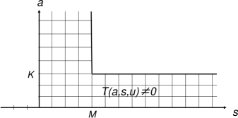
Figure 1: The domain (“fat hook”) of non-vanishing transfer matrices $T(a,s,u)$ for the supersymmetric spin chain with the $gl(K|M)$ symmetry.

We consider integrable generalized spin chains with $gl(K|M)$-invariant $R$-matrix. The generating function of commuting integrals of motion is the quantum transfer matrix $T^{(\lambda)}(u)$, which depends on the spectral parameter $u\in{\mathbb{C}}$ and the Young diagram $\lambda$. It is obtained as the (super)trace of the quantum monodromy matrix ${\cal T}^{(\lambda)}(u)$ in the auxiliary space carrying the irreducible representation of the symmetry algebra labeled by $\lambda$:

$$T^{(\lambda)}(u)=\mbox{str}_{{\rm aux}}\,{\cal T}^{(\lambda)}(u)\,.$$

We deal with covariant tensor irreducible representations (irreps) of the superalgebra.

The transfer matrices for different $\lambda$ are known to be functionally dependent. For rectangular diagrams $\lambda=(s^{a})$ with $a$ rows and $s$ columns the functional relation takes the form of the famous Hirota difference equation:

$$T(a,s,u\!+\!1)T(a,s,u\!-\!1)-T(a,s\!+\!1,u)T(a,s\!-\!1,u)=T(a\!+\!1,s,u)T(a\!-\!1,s,u),$$ (1.1)

where the transfer matrix for rectangular diagrams, after some $a,s$-dependent shift of the spectral parameter $u$, is denoted by $T(a,s,u)$. We see that it enters the equation as the $\tau$-function [29]. Since all the $T$’s commute, the same relation holds for their eigenvalues. We use the normalization in which all non-vanishing $T$’s are polynomials in $u$ of degree $N$, where $N$ is the number of sites in the spin chain.

While the functional relation is the same for ordinary and super-algebras, the boundary conditions are different. In the $gl(K)$-case, the domain of non-vanishing $T$’s in the $(s,a)$ plane is the half-strip $s\geq 0$, $0\leq a\leq K$. In the $gl(K|M)$-case, the domain of non-vanishing $T$’s has the form of a “fat hook”. It is shown in Fig. 1. To ensure compatibility with the Hirota equation, the boundary values at $s=0$ and $a=0$ should be rather special. In our normalization,

$$T(0,s,u)=\phi(u-s)\,,\quad\quad T(a,0,u)=\phi(u+a)\,,$$ (1.2)

where $\phi(u)=\prod_{i}(u-\theta_{i})$ is a fixed polynomial of degree $N$ which characterizes the spin chain.

Our goal is to solve the Hirota equation, with the boundary conditions given above, using the classical methods of the theory of solitons. This program for the case of ordinary Lie algebras (and for models with elliptic $R$-matrices) was realized in [16]. In this paper, we extend it to the case of superalgebras (for models with rational $R$-matrices).

One of the key features of soliton equations is the existence of (auto) Bäcklund transformations (BT), i.e., transformations that send any solution of a soliton equation to another solution of the same equation. A systematic way to construct such transformations is provided by considering an over-determined system of linear problems (called auxiliary linear problems) whose compatibility condition is the non-linear equation at hand. We introduce two Bäcklund transformations for the Hirota equation. They send any solution with the boundary conditions described above to a solution of the same Hirota equation with boundary conditions of the same fat hook type but with different $K$ or $M$. Specifically, one of them lowers $K$ by $1$ and the other one lowers $M$ by $1$ leaving all other boundaries intact. We call these transformations BT1 and BT2. Applying them successively $K+M$ times, one comes to a collapsed domain which is a union of two lines, the $s$-axis and the $a$-semi-axis shown in Fig.1, meaning that the original problem gets “undressed” to a trivial one. This procedure appears to be equivalent to the nested Bethe ansatz. Different orders in which we diminish $K$ and $M$ give raise to different “dual” systems of nested Bethe Ansatz equations. All of them describe the same system. They correspond to different choices of the basis of simple roots.

Let $k,m$ be indices running from $0$ to $K$ and from $0$ to $M$ respectively, and let $T_{k,m}(a,s,u)$ be the transfer matrices obeying the Hirota equation with the boundary conditions as above but with $K,M$ replaced by $k,m$. They are obtained from $T_{K,M}(a,s,u)$ by a chain of BT’s. Namely, $T_{k-1,m}$’s and $T_{k,m-1}$’s are solutions to the auxiliary linear problems for the Hirota equation for $T_{k,m}$’s:

$$\begin{CD}T_{k,m\!-\!1}@<{\rm BT2}<{}<T_{k,m}\\ @V{}V{\rm BT1}V\\ \;\;\;\;T_{k\!-\!1,m}\end{CD}$$

The explicit formulas of these transformations are given below (eq.(3.29) and eq.(3.30)). The functions $T_{k,m}(a,s,u)$ are polynomials in $u$ for any $a,s,k,m$ but the degree depends only on $k,m$. Let $Q_{k,m}(u)$ be the boundary values of the $T_{k,m}(a,s,u)$, i.e.,

$$T_{k,m}(0,s,u)=Q_{k,m}(u-s)\,,\quad\quad T_{k,m}(a,0,u)=Q_{k,m}(u+a)\,.$$

However, they are not fixed for the values of $k,m$ other than $k=K$, $m=M$ (when $Q_{K,M}(u)=\phi(u)$) and $k=m=0$ (when $Q_{0,0}(u)$ is put equal to $1$) but are to be determined from a solution to the hierarchy of Hirota equations. In fact these $Q$’s are Baxter polynomial functions whose roots obey the Bethe equations.

The result of a successive application of the transformations BT1 and BT2 does not depend on their order. This fact can be reformulated as a discrete zero curvature condition

$$\hat{U}_{k,m+1}^{-1}\hat{V}_{k,m}=\hat{V}_{k+1,m}\hat{U}_{k,m}^{-1}$$ (1.3)

for the shift operators in $k$ and $m$:

$$\hat{U}_{k,m}(u) = \frac{Q_{k+1,m}(u)\,Q_{k,m}(u\!+\!2)}{Q_{k+1,m}(u\!+\!2)\,Q_{k,m}(u)}\,-\,\,e^{2\partial_{u}},$$

$$\hat{V}_{k,m}(u) = \frac{Q_{k,m}(u)\,Q_{k,m+1}(u\!+\!2)}{Q_{k,m}(u\!+\!2)\,Q_{k,m+1}(u)}\,-\,\,e^{2\partial_{u}}.$$ (1.4)

Relation (1.3) is equivalent to the following Hirota equation for the Baxter $Q$-functions:

$$Q_{k,m}(u)Q_{k+1,m+1}(u+2)-Q_{k+1,m+1}(u)Q_{k,m}(u+2)=Q_{k,m+1}(u)Q_{k+1,m}(u+2).$$ (1.5)

This equation represents our principal new result. By analogy with Baxter’s $TQ$-relations, we call eq. (1.5) the $QQ$-relation. It provides the most transparent way to derive different systems of Bethe equations for the generalized spin chain and “duality transformations” between them. We also show that a number of more general Hirota equations of the similar type (i.e., acting in the space spanned by $k,m$ and a particular linear combination of $a,s,u$) hold for the full set of functions $T_{k,m}(a,s,u)$. They lead to a system of algebraic equations for their roots which generalizes the system of Bethe equations.

The transfer matrices can be expressed through the $Q$-functions via generalized Baxter’s $TQ$-relations. A simple way to represent them is to consider the (non-commutative) generating series of the transfer matrices for one-row diagrams,

$$\hat{W}_{k,m}(u)=Q_{k,m}^{-1}(u)\sum_{s=0}^{\infty}T_{k,m}(1,s,u\!+\!s\!+\!1)\,e^{2s\partial_{u}},$$ (1.6)

where the factor in front of the sum is put here for the proper normalization. The operator $\hat{W}$ is similar to the wave (or dressing) operator in the Toda lattice theory. We prove the following fundamental operator relations:

$$\hat{W}_{k+1,m}=\hat{U}_{k,m}^{-1}\hat{W}_{k,m}\,,\quad\quad\hat{W}_{k,m+1}=\hat{V}_{k,m}\hat{W}_{k,m}\,,$$ (1.7)

which implement the Bäcklund transformations on the level of the generating series. These relations allow one to represent $\hat{W}_{K,M}$ (the quantity of prime interest) as an ordered product of the operators $\hat{U}_{k,m}^{-1}$ and $\hat{V}_{k,m}$ along a zigzag path from the point $(0,0)$ to the point $(K,M)$ on the $(k,m)$ lattice. This representation provides a concise form of the generalized Baxter relations. Different zigzag paths correspond to different choices of the basis of simple roots, i.e., to different “dual” forms of supersymmetric Bethe equations (see Fig.17).

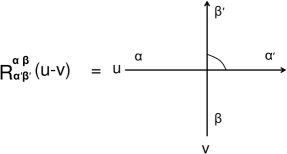
Figure 2: The $R$-matrix.

The normalization (1.2), with the roots $\theta_{i}$ of the polynomial $\phi(u)$ being in general position, implies that the “spins” of the inhomogeneous spin chain belong to the vector representation of the algebra $gl(K|M)$. Higher representations can be obtained by fusing of several copies of the vector ones. According to the fusion procedure, the corresponding $\theta$’s must be chosen in a specific “string-like” way which means that the differences between them are even integers constrained also by some more specific requirements. This amounts to the fact that the $Q$-functions become divisible by certain polynomials with explicitly prescribed roots located according to a similar string-like pattern. If one redefines the $Q$-functions dividing them by these normalization factors, then the $QQ$-relation gets modified and leads, in the same way as before, to the systems of Bethe equations with non-trivial right hand sides (sometimes called “vacuum parts”).

In section 7, we specify our construction for two popular examples, the $gl(1|1)$ and $gl(2|1)$ superalgebras. We present the $TQ$- and $QQ$-relations for all possible types of $Q$-functions $Q_{km}(u)$ ($0<k\leq K,\quad 0<m\leq M$) as well as Bethe equations for all types of simple roots systems and representations of the superalgebra (including typical representations with a continuous component of the Kac-Dynkin label) and compare them with the results existing in the literature. In our formalism, the construction becomes rather transparent and algorithmic. In this respect, our method is an interesting alternative to the algebraic Bethe ansatz approach.

2 Fusion relations for transfer matrices and Hirota equation

2.1 Quantum transfer matrices

Let $V={\mathbb{C}}^{K}\oplus{\mathbb{C}}^{M}\equiv{\mathbb{C}}^{K|M}$ be the graded linear space of the vector representation of the superalgebra $gl(K|M)$. The fundamental $gl(K|M)$-invariant rational $R$-matrix acts in $V\otimes V$ and has the form [1, 2]

$$R(u)=uI+2{\mit\Pi}=uI+2\sum_{\gamma,\gamma^{\prime}=1}^{K+M}(-1)^{p(\gamma^{\prime})}E_{\gamma\gamma^{\prime}}\otimes E_{\gamma^{\prime}\gamma}\,.$$ (2.1)

Here $I$ is the identity operator and $\mit\Pi$ is the super-permutation, i.e., the operator such that ${\mit\Pi}(x\otimes y)=(-1)^{p(x)p(y)}y\otimes x$ for any homogeneous vectors $x,y\in V$, and $E_{\alpha\beta}$ are the generators of the (super)algebra. In components, they read

$$I^{\alpha\beta}_{\alpha^{\prime}\beta^{\prime}}=\delta_{\alpha\alpha^{\prime}}\delta_{\beta\beta^{\prime}}\,,\quad\quad{\mit\Pi}^{\alpha\beta}_{\alpha^{\prime}\beta^{\prime}}=(-1)^{p(\alpha)p(\beta)}\delta_{\alpha\beta^{\prime}}\delta_{\alpha^{\prime}\beta}\,,\quad\quad(E_{\gamma\gamma^{\prime}})^{\alpha}_{\alpha^{\prime}}=\delta_{\alpha\gamma}\delta_{\alpha^{\prime}\gamma^{\prime}}\,.$$

Note that $\mit\Pi^{2}=I$, as in the ordinary case. The notation $p(x)$ is used to denote parity of the object $x$ (see Appendix A). The $R(u)$ has only even matrix elements. The complex variable $u$ is called the spectral parameter. The $R$-matrix obeys the graded Yang-Baxter equation (Fig. 3):

$$\begin{array}[]{ll}&\displaystyle{\sum_{\gamma\gamma^{\prime}\gamma^{\prime\prime}}(-1)^{p(\gamma^{\prime})(p(\alpha^{\prime\prime})+p(\gamma^{\prime\prime}))}R^{\alpha\alpha^{\prime}}_{\gamma\gamma^{\prime}}(u-v)R^{\gamma\alpha^{\prime\prime}}_{\beta\gamma^{\prime\prime}}(u)R^{\gamma^{\prime}\gamma^{\prime\prime}}_{\beta^{\prime}\beta^{\prime\prime}}(v)}\\ &\\ =&\displaystyle{\sum_{\gamma\gamma^{\prime}\gamma^{\prime\prime}}(-1)^{p(\gamma^{\prime})(p(\beta^{\prime\prime})+p(\gamma^{\prime\prime}))}R^{\alpha^{\prime}\alpha^{\prime\prime}}_{\gamma^{\prime}\gamma^{\prime\prime}}(v)R^{\alpha\gamma^{\prime\prime}}_{\gamma\beta^{\prime\prime}}(u)R^{\gamma\gamma^{\prime}}_{\beta\beta^{\prime}}(u-v)}\end{array}$$ (2.2)

This is the key relation to construct a family of commuting operators, as is outlined below.

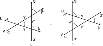
Figure 3: The Yang-Baxter equation.

The $R$-matrix is an operator in the tensor product of two linear spaces (not necessarily isomorphic). It is customary to call one of them quantum and the other one auxiliary space. In Fig. 2 they are associated with the vertical and the horizontal lines respectively. Let us fix a set of $N$ complex numbers $\theta_{i}$ and consider a chain of $N$ fundamental $R$-matrices $R(u-\theta_{i})$ with the common auxiliary space $V$. Multiplying them as linear operators in $V$ along the chain, we get an operator in $V^{\otimes N}$ which is called quantum monodromy matrix. In components, it can be written as

$${\cal T}^{\gamma_{0},\{\alpha_{i}\}}_{\gamma_{N},\{\beta_{i}\}}(u)=\!\!\!\sum_{\gamma_{1},\ldots,\gamma_{N-1}}R^{\gamma_{N-1}\alpha_{N}}_{\gamma_{N}\beta_{N}}(u\!-\!\theta_{N})\ldots R^{\gamma_{1}\alpha_{2}}_{\gamma_{2}\beta_{2}}(u\!-\!\theta_{2})R^{\gamma_{0}\alpha_{1}}_{\gamma_{1}\beta_{1}}(u\!-\!\theta_{1})\,(-1)^{\sum_{i=2}^{N}[p(\alpha_{i})+p(\beta_{i})]\sum_{j=1}^{i-1}p(\alpha_{j})}$$ (2.3)

It is usually regarded as an operator-valued matrix in the auxiliary space (with indices $\gamma_{0}$, $\gamma_{N}$), with the matrix elements being operators in the quantum space $V^{\otimes N}$ (see Fig. 4). Setting $\gamma_{0}=\gamma_{N}=\gamma$ and summing with the sign factor $(-1)^{p(\gamma)}$, we get the supertrace of the quantum monodromy matrix in the auxiliary space,

$$T(u)=\,\mbox{str}\,{\cal T}(u)=\sum_{\gamma}(-1)^{p(\gamma)}{\cal T}^{\gamma}_{\gamma}(u)$$ (2.4)

which is an operator in the quantum space (indices of the quantum space are omitted). It is called the quantum transfer matrix. Using the graded Yang-Baxter equation, it can be shown that the $T(u)$ commute at different $u$: $[T(u),\,T(u^{\prime})]=0$. Their diagonalization is the subject of one or another version of Bethe ansatz.

The (inhomogeneous) integrable “spin chain” or a vertex model on the square lattice is characterized by the symmetry algebra $gl(K|M)$ and the parameters $\theta_{i}$ (inhomogeneities at the sites or “rapidities”). Given such a model, the family of transfer matrices $T(u)$ (2.4) can be included into a larger family of commuting operators. It is constructed by means of the fusion procedure.

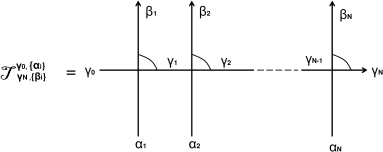
Figure 4: The monodromy matrix.

2.2 Fusion procedure

Using the $R$-matrix (2.1) as a building block, it is possible to generate other $gl(K|M)$-invariant solutions to the (graded) Yang-Baxter equation. They are operators in tensor products of two arbitrary finite dimensional irreps of the symmetry algebra. We consider covariant tensor irreps which are labeled (although in a non-unique way, see Appendix A) by Young diagrams $\lambda$. Let $V_{\lambda}$ be the corresponding representation space, then the $R$-matrix acts in $V_{\lambda}\otimes V_{\lambda^{\prime}}$. The construction of this $R$-matrix from the elementary one is referred to as fusion procedure [7, 32], [33]-[36].

Here we consider fusion in the auxiliary space, which allows one to construct, by taking (super)trace in this space, a large family of transfer matrices commuting with $T(u)$. In words, the fusion procedure consists in tensor multiplying several copies of the fundamental $R$-matrix (2.1) in the auxiliary space and subsequent projection onto an irrep of the $gl(K|M)$ algebra. As a result, one obtains an $R$-matrix $R^{(\lambda)}(u)$ whose quantum space is still $V$ (the space of the vector representation of $gl(K|M)$) and whose auxiliary space is the space $V_{\lambda}$ of a higher irrep $\lambda$ of this algebra. The fact that the $R$-matrix obtained in this way obeys the (graded) Yang-Baxter equation follows from the observation [7, 34] that the projectors onto higher irreps can be realized as products of the fundamental $R$-matrices (2.1) taken at special values of the spectral parameter. These values correspond to the degeneration points of the $R$-matrices.

In particular, the $R$-matrix (2.1) has two degeneration points $u=\pm 2$. Indeed, one can easily see that

$$\det R(u)=(u+2)^{d_{+}}(u-2)^{d_{-}}\,,\quad d_{\pm}=\frac{1}{2}((K+M)^{2}\pm(K-M))\,,$$ (2.5)

$$R(\pm 2)=\pm 2(I\pm{\mit\Pi})=\pm 4P_{\pm}\,,$$ (2.6)

where $P_{\pm}$ are projectors onto the symmetric and antisymmetric subspaces in $V\otimes V$. The dimensions of these subspaces are equal to $d_{\pm}$, and the projectors are complimentary, i.e., $P_{+}P_{-}=P_{-}P_{+}=0$. Therefore, to get the $R$-matrix with the auxiliary space carrying the $\lambda=(2^{1})$ irrep (respectively, the $\lambda=(1^{2})$ irrep), one should take the tensor product $R(u+2)\otimes R(u)$ (respectively, $R(u-2)\otimes R(u)$) in the auxiliary space and apply the projector $P_{+}$ (respectively, $P_{-}$):

$$R^{(2^{1})}(u)=P_{+}\Bigl{[}R(u+2)\otimes R(u)\Bigr{]}P_{+}\,,\quad R^{(1^{2})}(u)=P_{-}\Bigl{[}R(u-2)\otimes R(u)\Bigr{]}P_{-}\,.$$

Here, the tensor product notation still implies the usual matrix product in the quantum space. Note that $R^{(2^{1})}(-2)$ vanishes identically since the projector $P_{+}$ gets multiplied by the complementary projector $P_{-}$ coming from one of the $R$-matrices in the tensor product. Similarly, $R^{(1^{2})}(2)=0$.

In a more general case, the procedure is as follows. Let $\lambda$ be the Young diagram associated with a given irrep of the algebra. Let $n=|\lambda|$ be the number of boxes in the diagram and let

$$P_{\lambda}:\left({\mathbb{C}}^{K|M}\right)^{\otimes n}\longrightarrow V_{\lambda}$$

be the projector onto the space of the irreducible representation. Write in the box with coordinates $(i,j)$ ($i$-th line counting from top to bottom and $j$-th column counting from left to right) the number $u_{ij}=u-2(i-j)$, as is shown in Fig. 5. Then $R^{(\lambda)}(u)$ is constructed as

$$R^{(\lambda)}(u)=P_{\lambda}\Bigl{[}\bigotimes_{(ij)\in\lambda}^{\longleftarrow}R(u_{ij})\Bigr{]}\,\,P_{\lambda}$$ (2.7)

Here, the tensor factors are placed from right to left in the lexicographical order, i.e., elements of the first row from left to right, then elements of the second row from left to right, etc. For example, for the diagram $\lambda=(3,2)$ the product under the projectors reads $R(u)\otimes R(u-2)\otimes R(u+4)\otimes R(u+2)\otimes R(u)$.

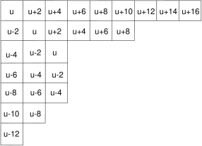
Figure 5: The Young diagram decorated by spectral parameters.

Omitting further details of the fusion procedure (see, e.g., [35, 36]), we now describe the structure of zeros of the fused $R$-matrix $R^{(\lambda)}(u)$ which is essential for what follows. As we have seen, the $R$-matrix $R^{(\lambda)}(u)$ is obtained by fusing $n=|\lambda|$ fundamental $R$-matrices in the auxiliary space. Then, by the construction, any matrix element of the $R^{(\lambda)}(u)$ is a polynomial in $u$ of degree $\leq n$. However, one can see that at some special values of the spectral parameter the complimentary projectors get multiplied and the matrix $R^{(\lambda)}(u)$ vanishes as a whole thing. In other words, the matrix elements have a number of common zeros. We call them “trivial zeros”. A more detailed analysis shows that the number of trivial zeros is $n-1$ (counting with multiplicities) and thus a scalar polynomial of degree $n-1$ can be factored out. Namely, this polynomial is equal to the product of the factors $u_{ij}=u-2(i-j)$ over the boxes of the diagram $\lambda$ with $(i,j)\in\lambda$ except $i=j=1$.

We consider here only the representations of the type $\lambda=(s^{a})$ corresponding to rectangular Young diagrams with $s$ rows and $a$ columns (rectangular irreps). In this case

$$R^{(s^{a})}(u)=r_{a,s}(u)\,{\sf R}^{(s^{a})}(u)\,,$$

where matrix elements of ${\sf R}^{(s^{a})}(u)$ are polynomials of degree $\leq 1$ and

$$r_{a,s}(u)=u^{-1}\prod_{j=1}^{s}\prod_{l=1}^{a}(u+2j-2l)\,,\quad\quad a,s\geq 1,$$ (2.8)

is the polynomial of degree $as-1$. For a future reference, we give its representation through the Barnes function $G(z)$ (a unique entire function such that $G(z+1)=\Gamma(z)G(z)$ and $G(1)=1$):

$$r_{a,s}(u)=2^{as}\,u^{-1}\,\frac{G(\frac{1}{2}u+s+1)\,G(\frac{1}{2}u-a+1)}{G(\frac{1}{2}u+1)\,\,G(\frac{1}{2}u+s-a+1)}\,.$$ (2.9)

The quantum monodromy matrix ${\cal T}^{(\lambda)}$ with the auxiliary space $V_{\lambda}$ is defined by the same formula as before but with the $R$-matrix $R^{(\lambda)}$. The transfer matrix is

$$T^{(\lambda)}(u)=\,\mbox{str}_{V_{\lambda}}{\cal T}^{(\lambda)}(u)$$ (2.10)

The transfer matrices commute for any $\lambda$ and $u$: $[T^{(\lambda)}(u),\,T^{(\lambda^{\prime})}(u^{\prime})]=0$. This commuting family of operators extends the family (2.4) which corresponds to the one-box diagram $\lambda$. For the empty diagram $\lambda=\emptyset$ we formally put $T^{(\emptyset)}(u)=1$. For rectangular diagrams $\lambda=s^{a}$ we use the special notation $T^{(\lambda)}(u):=T^{a}_{s}(u)$.

2.3 Functional relations for transfer matrices

The transfer matrices are functionally dependent. It appears that all $T^{(\lambda)}(u)$ can be expressed through $T^{1}_{s}(u)$ or $T^{a}_{1}(u)$ by means of the nice determinant formulas due to Bazhanov and Reshetikhin [9]. They are the same for all (super)algebras of the type $gl(K|M)$ with $K,M\geq 0$ [12]:

$$\begin{array}[]{lll}T^{(\lambda)}(u)&=&\displaystyle{\det_{1\leq i,j\leq\lambda_{1}^{\prime}}T^{1}_{\lambda_{j}+i-j}(u-2i+2)}\\ &&\\ &=&\displaystyle{\det_{1\leq i,j\leq\lambda_{1}}T^{\lambda_{j}^{\prime}+i-j}_{1}(u+2i-2)}\,.\end{array}$$ (2.11)

For rectangular diagrams, they read:

$$\begin{array}[]{lll}T^{a}_{s}(u)&=&\displaystyle{\det_{1\leq i,j\leq a}T^{1}_{s+i-j}(u-2i+2)}\\ &&\\ &=&\displaystyle{\det_{1\leq i,j\leq s}T^{a+i-j}_{1}(u+2i-2)}\,.\end{array}$$ (2.12)

These formulas should be supplemented by the “boundary conditions” $T^{0}_{s}(u)=T^{a}_{0}(u)=1$, $T^{-n}_{s}(u)=T^{a}_{-n}(u)=0$ for all $a,s\geq 0$ and $n\geq 1$. Since all the transfer matrices commute, they can be diagonalized simultaneously, and the same relations are valid for any of their eigenvalues. Keeping this in mind, we will often refer to the transfer matrices as scalar functions and call them “$T$-functions”.

Applying the Jacobi identity for determinants to formulas (2.12) (see, e.g., [37, 16]), one obtains a closed functional relation between transfer matrices for rectangular diagrams, equivalent to Hirota difference equation:

$$T^{a}_{s}(u-2)T^{a}_{s}(u)-T^{a}_{s+1}(u-2)T^{a}_{s-1}(u)=T^{a-1}_{s}(u-2)T^{a+1}_{s}(u)$$ (2.13)

The bilinear form of the functional relations was discussed in [10], [11], [16], [37]-[40]. Below we illustrate this relation by simple examples.

2.3.1 Simple examples of the functional equation

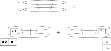
Figure 6: Fusion of two fundamental transfer matrices and the corresponding Hirota equation. As usual, each line carries the vector representation, each crossing corresponds to the insertion of the $R$-matrix, and the closed lines correspond to taking traces in the auxiliary space. The insertions of projectors $P^{\pm}$ are interpreted as insertions of the $R$-matrices with given values of spectral parameters.

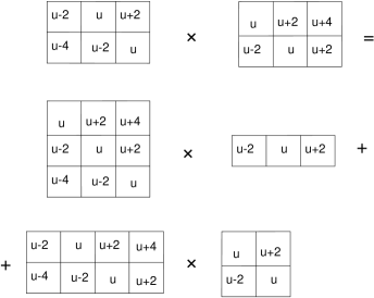
Figure 7: The Hirota-type relation illustrated by rectangular Young diagrams decorated by spectral parameters. To obtain the first term in the r.h.s., one takes the first row of the second diagram in the l.h.s. and puts it on the top of the first one. To obtain the second term in the r.h.s., one takes the first column of the first diagram in the l.h.s. and attaches it to the second one from the left.

To figure out the general pattern, it is useful to consider the simplest case of the fusion of two transfer matrices with fundamental representations in the auxiliary space. The proof is summarized in Fig. 6. Let us represent the first term in eq.(2.13) as

$$T_{1}^{1}(u-2)T_{1}^{1}(u)={\rm tr}_{{\rm aux}\,,\,V\otimes V}\left[{\cal T}_{20}(u-2){\cal T}_{10}(u)\right]$$ (2.14)

The index $0$ denotes the common quantum space represented in the figure by several vertical lines, the indices $1,2$ denote the two copies of the auxiliary space $V$. Inserting $I=P_{+}+P_{-}$ inside the trace, we get two terms. Using the projector property $P_{\pm}^{2}=P_{\pm}$, we immediately see that the term with $P_{+}$ is equal to $T_{2}^{1}(u-2)$, by the definition of the latter. The term with $P_{-}$ does not literally coincide with the definition of $T_{1}^{2}(u)$ since the order of the horizontal lines is reversed. However, plugging $P_{-}=-\frac{1}{4}R(-2)$ and using the Yang-Baxter equation to move the vertical lines to the other side of the $R$-matrix $R(-2)$, we come to the equivalent graph with the required order of the horizontal lines. Finally, we get

$$T_{1}^{1}(u-2)T_{1}^{1}(u)=T_{2}^{1}(u-2)+T_{1}^{2}(u)\,.$$ (2.15)

Hence we have reproduced the simplest case of eq.(2.13).

Let us comment on the general case. An illustrative example is given in fig.7. The rectangular Young diagrams are decorated by the values of the spectral parameter

$$u_{ij}=u-2(i-j),$$ (2.16)

as is explained above. Each box of such decorated diagrams corresponds to a line characterized by a given value of the spectral parameter. All these lines cross each other and the $R$-matrices are associated to the crossing points. The order of the crossings is irrelevant due to the Yang-Baxter equation. The reshuffling of spectral parameters in the second and third terms of equation (2.13) (corresponding to the second and the third lines in the figure) is done by the exchange of a row or a column between the two diagrams of the first line. The decoration of the resulting Young diagrams follows the rule (2.16). Of course this is not a proof, just an illustration.

2.3.2 Analogy with formulas for characters and identities for symmetric functions

Equations (2.11) are spectral parameter dependent versions of the second Weyl formula for characters of (super)groups (see [20]):

$$\chi_{\lambda}(w_{1},\dots,w_{K};v_{1},\dots,v_{M})=\det_{i,j=1,\dots,K+M}S_{\lambda_{i}+i-j}\,.$$ (2.17)

In the theory of symmetric functions such formulas are known as the Jacobi-Trudi determinant identities. Here $\lambda_{i}$ are the lengths of the rows of the diagram $\lambda$, $S_{n}$ are super Schur polynomials defined as

$$\frac{\prod_{m=1}^{M}\left(1-zv_{m}\right)}{\prod_{k=1}^{K}\left(1-zw_{k}\right)}=\sum_{n=1}^{\infty}z^{n}S_{n},$$ (2.18)

and $w_{k}$, $v_{m}$ are eigenvalues of the $A$- and $D$-parts of the diagonalized element of the supergroup in the matrix realization of the type (A1).

For the rectangular irrep with $\lambda=s^{a}$ eq. (2.17) reads

$$\chi_{s^{a}}\equiv\chi(a,s)=\det_{i,j=1,\dots,a}S_{s+i-j}.$$ (2.19)

The characters $\chi_{s^{a}}$ satisfy the bilinear relation

$$\chi^{2}(a,s)=\chi(a+1,s)\chi(a-1,s)+\chi(a,s+1)\chi(a,s-1)$$ (2.20)

which follows from the Jacobi identity for determinants. It is the spectral parameter independent version of the Hirota equation.

2.3.3 Normalization and boundary conditions

A simple redefinition of the $T$-functions by a shift of the spectral parameter,

$$T^{(a,s)}(u)\equiv T^{a}_{s}(u-s+a)$$ (2.21)

brings equation (2.13) to the form

$$T^{(a,s)}(u+1)T^{(a,s)}(u-1)-T^{(a,s+1)}(u)T^{(a,s-1)}(u)=T^{(a+1,s)}(u)T^{(a-1,s)}(u)$$ (2.22)

which appears to be completely symmetric with respect to interchanging of $a$ and $s$. This is the famous Hirota bilinear difference equation [18] which is the starting point of our approach to the Bethe ansatz and generalized Baxter equations in this paper. For convenience, we also give the determinant representation (2.12) in terms of $T^{(a,s)}(u)$:

$$\begin{array}[]{lll}T^{(a,s)}(u)&=&\displaystyle{\det_{1\leq i,j\leq a}T^{(1,\,s+i-j)}(u+a+1-i-j)}\\ &&\\ &=&\displaystyle{\det_{1\leq i,j\leq s}T^{(a+i-j,\,1)}(u+s+1-i-j)}\,.\end{array}$$ (2.23)

Let us comment on the meaning of equation (2.22). On the first glance, there is no much content in this equation. Its general solution (with the boundary conditions fixed above) is just given by formulas (2.23) with arbitrary functions $T^{(1,s)}(u)$ or $T^{(a,1)}(u)$. However, in the problem of interest these functions are by no means arbitrary. They are to be found from certain analytic conditions. For the finite spin chains with finite dimensional representations at each site these conditions simply mean that $T^{(a,s)}(u)$ must be a polynomial of degree $asN$, where $N$ is the length of the chain, with $(as-1)N$ fixed zeros. These zeros are just the trivial zeros coming from the fusion procedure. Their location is determined by the scalar factor $r_{a,s}(u)$ (2.8) of the $R$-matrix. We thus see that the polynomial $T^{(a,s)}(u)$ for all $a,s\geq 1$ must be divisible by the polynomial

$$\prod_{i=1}^{N}r_{a,s}(u-s+a-\theta_{i}):=\Phi(a,s,u)\,.$$

This constraint makes the problem non-trivial.

Let us introduce the function

$$\phi(u)=\prod_{i=1}^{N}(u-\theta_{i})\,,$$ (2.24)

in terms of which the scalar polynomial factor is written as

$$\Phi(a,s,u)=\prod_{i=1}^{N}r_{a,s}(u-s+a-\theta_{i})=\phi^{-1}(u-s+a)\prod_{j=1}^{s}\prod_{l=1}^{a}\phi(u-s+a+2j-2l)\,,\quad a,s\geq 1.$$

The representation through the Barnes function (2.9) allows us to extend this formula to all values of $a$ and $s$:

$$\Phi(a,s,u)=2^{asN}\phi^{-1}(u\!-\!s\!+\!a)\,\prod_{i=1}^{N}\frac{G\left(\frac{1}{2}(u+s+a)+1-\theta_{i}\right)\,G\left(\frac{1}{2}(u-s-a)+1-\theta_{i}\right)}{G\left(\frac{1}{2}(u-s+a)+1-\theta_{i}\right)\,G\left(\frac{1}{2}(u+s-a)+1-\theta_{i}\right)}$$ (2.25)

Extracting it from the $T^{(a,s)}(u)$, we introduce the $T$-function

$$T(a,s,u)=\Phi^{-1}(a,s,u)\,T^{(a,s)}(u)$$ (2.26)

which is a polynomial in $u$ of degree $N$ for all $a,s\geq 0$. Note that at $a=0$ or $s=0$ equation (2.25) yields $\Phi(0,s,u)=1/\phi(u-s)$, $\Phi(a,0,u)=1/\phi(u+a)$, so

$$T(0,s,u)=\phi(u-s)\,,\quad\quad T(a,0,u)=\phi(u+a)\,.$$ (2.27)

It is important to note that the renormalized $T$-function $T(a,s,u)$ obeys the same Hirota equation (2.22) as the $T$-function $T^{(a,s)}(u)$. Indeed, it easy to check that the transformation

$$T^{(a,s)}(u)\longrightarrow f_{0}(u\!+\!s\!+\!a)f_{1}(u\!+\!s\!-\!a)f_{2}(u\!-\!s\!+\!a)f_{3}(u\!-\!s\!-\!a)T^{(a,s)}(u),$$ (2.28)

where $f_{i}$ are arbitrary functions, leaves the form of the equation unchanged. Equation ((2.25)) shows that the function $\Phi(a,s,u)$ is precisely of this form (the factor $2^{asN}$ is easily seen to be of this form, too).

The main difference between the “bosonic” $gl(K)$ and supersymmetric $gl(K|M)$ cases is in the boundary conditions for the transfer matrices in the $(s,a)$-plane. For the algebra $gl(K)$ the rectangular Young diagrams live in the half-band $s\geq 0$, $0\leq a\leq K$, while for the superalgebra the rectangular diagrams live in the domain shown below in Fig. 9. The Hirota equation with boundary conditions of this type will be our starting point for the analysis of the inhomogeneous quantum integrable super spin chains and it will allow us to obtain the full hierarchy of Baxter relations, the new Hirota equation for the Baxter functions and the nested Bethe ansatz equations for all possible choices of simple root systems for $gl(K|M)$. This naturally generalizes the known relations for the spin chains based on the $gl(K)$ algebra.

3 Hierarchy of Hirota equations

Throughout the rest of the paper we deal with rectangular irreps only and use the normalization (2.26), where all the “trivial” zeros of the transfer matrix are excluded. This normalization was used in [16, 17], for the supersymmetric case see [15].

3.1 Hirota equation and boundary conditions for superalgebra $gl(K|M)$

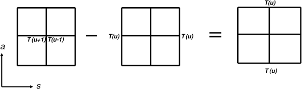
Figure 8: Hirota equation in the $(s,a)$-plane.

As we have seen in the previous section, the functional relations for transfer matrices of integrable quantum spin chains with “spins” belonging to representations of the superalgebra $gl(K|M)$ can be written [12] in the form of the same Hirota equation as in the case of the ordinary Lie algebra $gl(K)$:

$$T(a,s,u\!+\!1)T(a,s,u\!-\!1)-T(a,s\!+\!1,u)T(a,s\!-\!1,u)=T(a\!+\!1,s,u)T(a\!-\!1,s,u).$$ (3.1)

It can be schematically drawn in the $(s,a)$-plane as is shown in Fig. 8. All the non-vanishing $T(a,s,u)$’s are polynomials in $u$ of one and the same degree $N$ equal to the number of sites in the spin chain.

To distinguish solutions relevant to Bethe ansatz for a given (super)algebra, one should specify the boundary conditions in the discrete variables $a$ and $s$. For the superalgebra $gl(K|M)$ one can see [41, 12] that

$$T(a,s,u)=0\quad{\rm if:}\quad\mbox{(i)}\;\;a<0\quad{\rm or}\quad\mbox{(ii)}\;\;s<0\;\;{\rm and}\;\;a\neq 0,\quad{\rm or}\quad\mbox{(iii)}\;\;a>K\;\;{\rm and}\;\;s>M.$$ (3.2)

(see Fig. 9, where we use the letters $k,m$ rather than $K,M$ for later references). The latter requirement, that $T(a,s,u)$ vanishes if simultaneously $a>K$ and $s>M$, comes from the fact that the Young superdiagrams for $gl(K|M)$ containing a rectangular subdiagram with $K+1$ rows and $M+1$ columns are illegal, i.e., the corresponding representations vanish [21]. Note that we want the Hirota equation to be valid in the whole $(s,a)$ plane, not just in the quadrant $a,s\geq 1$. This is why we have to require that $T(0,s,u)$ does not vanish identically on the negative $s$-axis, otherwise the Hirota equation would break down at the origin $a=s=0$.

The boundary values of $T(a,s,u)$ are rather special. For example, at $a=0$ eq. (3.1) converts into

$$T(0,s,u\!+\!1)T(0,s,u\!-\!1)=T(0,s\!+\!1,u)T(0,s\!-\!1,u)$$

which is a discrete version of the d’Alembert equation with the general solution $T(0,s,u)=f_{+}(u+s)f_{-}(u-s)$ where $f_{\pm}$ are arbitrary functions. In the normalization (2.26) we have $f_{+}(u)=1$, $f_{-}(u)=\phi(u)$ (see (2.27)). Similarly, the boundary function at the half-axis $s=0,a\geq 0$ is normalized to depend on $u+a$ only in which case it has to be equal to $f_{-}(u+a)=\phi(u+a)$. As soon as this is fixed, there is no more freedom left, and the boundary functions at the interior boundaries are in general products of a function of $u+s$ and a function of $u-s$ on the horizontal line (respectively, of $u+a$ and $u-a$ on the vertical line). One more thing to be taken into account is the identification (up to a sign) of the $T$-functions on the two interior boundaries:

$$T(K,M+n,u)=(-1)^{nM}T(K+n,M,u),\quad n\geq 0.$$ (3.3)

This equality reflects the fact that the two rectangular Young diagrams of the shapes $\left((M\!+\!n)^{K}\right)$ and $(M^{K+n})$ correspond to the same representation of the algebra $gl(K|M)$ with the Kac-Dynkin label $b_{1}=\ldots=b_{K-1}=0$, $b_{K}=M+n$, $b_{K+1}=\ldots=b_{K+M-1}=0$ [21]. Note also that every point with integer coordinates inside the domain in Fig. 9 corresponds to an atypical representation while the points on the interior boundaries correspond to typical ones, and in this respect the coordinate along the boundary can be treated as a continuous number.

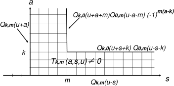
Figure 9: Boundary conditions for the Hirota equation in the case of the superalgebra $gl(k|m)$. Note that $T(0,s,u)=Q_{k,m}(u-s)\neq 0$ on the whole axis $-\infty<s<+\infty$.

Summarizing, we can write:

$$T(0,s,u) = Q_{K,M}(u-s),\quad-\infty<s<\infty,$$

$$T(a,0,u) = Q_{K,M}(u+a),\quad 0\leq a<\infty,$$

$$T(K,s,u) = Q_{K,0}(u+s+K)Q_{0,M}(u-s-K),\quad M\leq s<\infty,$$

$$T(a,M,u) = (-1)^{M(a-K)}Q_{K,0}(u+a+M)Q_{0,M}(u-a-M),\quad K\leq a<\infty,$$ (3.4)

where the polynomial boundary function $Q_{K,M}(u)=\phi(u)$ is regarded as a fixed input characterizing the quantum space of the spin chain while the polynomials $Q_{K,0}(u)$ and $Q_{0,M}(u)$ are to be determined from the solution to the Hirota equation. At $K=M=0$ the domain of non-vanishing $T$’s shrinks to the axis $a=0$ and the half-axis $s=0$, $a\geq 0$, and the “gauge” freedom allows one to put $Q_{0,0}(u)=1$. It should be noted that the identification (3.3) does not yet imply the coincidence of the $Q$-functions in the third and the fourth lines of eq. (3.1) (i.e., on the horizontal and vertical parts of the interior boundary). In fact the specific form of the boundary conditions given in eq. (3.1) (as well as the sign factor $(-1)^{M(a-K)}$) is determined by a consistency with a more general hierarchy of Hirota equations connecting the $T$-functions for different values of $K$ and $M$. The uniqueness of the boundary conditions (3.1) will be justified in the next subsection.

In the case of the usual Lie algebra $gl(K)$ ($M=0$) the boundary conditions (3.1) become the same as the ones imposed in [17] (in the original paper [16] a gauge equivalent version was used). The domain of non-vanishing $T$’s in Fig. 9 degenerates so that the vertical strip collapses to a line. Therefore, the $T$-functions on the interior boundaries cease to be dynamical variables and become equal, up to a shift of the argument, to the fixed function $Q_{K,0}=\phi(u)$ characterizing the spin chain (see [16, 17]).

One of the possible setups of the problem is the following: we fix the polynomial $Q_{K,M}(u)$ and then solve the Hirota equation with the aforementioned boundary and analytic conditions. The result is a finite set of solutions for $T(a,s,u)$ which yield the spectrum of eigenvalues of the quantum transfer matrix. We proceed by constructing a hierarchy of Hirota equations connecting neighboring “levels” of the array in Fig. 9, i.e., equations connecting $T$-functions for which $K$ or $M$ differ by $1$. The existence of such a hierarchy follows from classical integrability of the Hirota equation. Decreasing $K$ and $M$ by $1$, one can “undress” step by step the original $gl(K|M)$ problem to an empty problem formally corresponding to $gl(0|0)$. This procedure appears to be equivalent to the hierarchial (nested) Bethe ansatz.

3.2 Auxiliary linear problems and Bäcklund transformations

Like almost all known nonlinear integrable equations, the Hirota equation (3.1) serves as a compatibility condition for over-determined linear problems [30, 16]. To introduce them, it is convenient to pass to the new variables

$$\begin{array}[]{l}p=\frac{1}{2}(u-s-a)\\ \\ q=\frac{1}{2}(u+s+a)\\ \\ r=\frac{1}{2}(-u-s+a)\end{array}$$ (3.5)

We call them “chiral” or “light-cone” variables while the original ones will be refered to as “laboratory” variables. Here are the formulas for the inverse transformation,

$$a=q+r\,,\quad s=-p-r\,,\quad u=p+q$$ (3.6)

and for the transformation of the vector fields:

$$\partial_{p}=\partial_{u}-\partial_{s}\,,\quad\partial_{q}=\partial_{u}+\partial_{a}\,,\quad\partial_{r}=\partial_{a}-\partial_{s}$$ (3.7)

We set $\tau(p,q,r)=T(q+r,\,-p-r,\,p+q)$ and introduce the following linear problems for an auxiliary function $\psi=\psi(p,q,r)$:

$$\begin{array}[]{l}\displaystyle{\left(e^{\partial_{r}}+\frac{\tau(p\!+\!1,r\!+\!1)\,\,\tau}{\tau(p+1)\tau(r+1)}\right)\psi=\psi(p+1)}\\ \\ \displaystyle{\left(e^{\partial_{r}}-\frac{\tau(q\!+\!1,r\!+\!1)\,\,\tau}{\tau(q+1)\tau(r+1)}\right)\psi=\psi(q+1)}\end{array}$$ (3.8)

where we indicate explicitly only those variables that are subject to shifts. The compatibility means that the difference operators

$$e^{-\partial_{p}}\left(e^{\partial_{r}}+\frac{\tau(p\!+\!1,r\!+\!1)\,\,\tau}{\tau(p+1)\tau(r+1)}\right)\quad\mbox{and}\quad\;e^{-\partial_{q}}\left(e^{\partial_{r}}-\frac{\tau(q\!+\!1,r\!+\!1)\,\,\tau}{\tau(q+1)\tau(r+1)}\right)$$

commute. This leads to the relation

$$\tau(p+1)\tau(q+1,r+1)+\tau(q+1)\tau(p+1,r+1)=h(2p,2q)\tau(r+1)\tau(p+1,q+1)$$

where $h$ can be an arbitrary function of $p$ and $q$. In the original variables this equation reads

$$T(a+1)T(a-1)+T(s+1)T(s-1)=h(u\!-\!s\!-\!a,u\!+\!s\!+\!a)\,T(u+1)T(u-1)$$

From the boundary conditions (3.1) at $a=0$ or $s=0$ it follows that $h=1$ and we obtain the Hirota equation (3.1).

An advantage of the “light-cone” variables is their separation in the linear problems: the first problem does not involve $q$ while the second one does not involve $p$. However, in contrast to the “laboratory” variables $a,s,u$, they have no immediate physical meaning. Coming back to the “laboratory” variables, we set $\psi(p,q,r)=\Psi(q+r,\,-p-r,\,p+q)$ and rewrite the linear problems (3.8) in the form

$$\begin{array}[]{l}\displaystyle{\left[e^{\partial_{a}-\partial_{s}}+\frac{T(a\!-\!1,s\!+\!1,u)T(a,s\!-\!1,u\!+\!1)}{T(a,s,u)\,T(a\!-\!1,s,u\!+\!1)}\right]\Psi(a\!-\!1,s\!+\!1,u)=\Psi(a\!-\!1,s,u\!+\!1)}\\ \\ \displaystyle{\left[e^{\partial_{a}-\partial_{s}}-\frac{T(a\!-\!1,s\!+\!1,u)T(a\!+\!1,s,u\!+\!1)}{T(a,s,u)\,T(a,s\!+\!1,u\!+\!1)}\right]\Psi(a\!-\!1,s\!+\!1,u)=\Psi(a,s\!+\!1,u\!+\!1)}\end{array}$$ (3.9)

Because the $T$-functions can vanish identically at some $a,s$, we eliminate the denominators by passing to the new auxiliary function $F=T\Psi$, in terms of which we have

$$\begin{array}[]{l}\displaystyle{T(a\!-\!1,s,u\!+\!1)F(a,s,u)\,+\,T(a,s\!-\!1,u\!+\!1)F(a\!-\!1,s\!+\!1,u)=T(a,s,u)F(a\!-\!1,s,u\!+\!1)}\\ \\ \displaystyle{T(a,s\!+\!1,u\!+\!1)F(a,s,u)\,-\,T(a\!+\!1,s,u\!+\!1)F(a\!-\!1,s\!+\!1,u)=T(a,s,u)F(a,s\!+\!1,u\!+\!1)}\end{array}$$ (3.10)

Note that the second equation can be obtained from the first one by the transformation $T(a,s,u)\longrightarrow(-1)^{as}T(-s,-a,u)$ (and the same for $F$) which leaves the Hirota equation invariant. Note also that the pair of equations can be written in a matrix form as follows:

$$\left(\begin{array}[]{cc}T(a\!-\!1,s,u)&T(a,s\!-\!1,u)\\ &\\ T(a,s\!+\!1,u)&-T(a\!+\!1,s,u)\end{array}\right)\left(\begin{array}[]{c}F(a,\,s,\,u\!-\!1)\\ \\ F(a\!-\!1,s\!+\!1,u\!-\!1)\end{array}\right)=T(a,s,u\!-\!1)\left(\begin{array}[]{c}F(a\!-\!1,s,u)\\ \\ F(a,s\!+\!1,u)\end{array}\right).$$ (3.11)

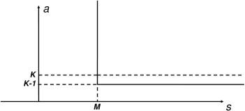
Figure 10: Boundary conditions for the first Bäcklund transformation in the $(s,a)$ plane.

A remark on the symmetry properties of the linear problems is in order. One can see that while the Hirota equation (3.1) written for the function $(-1)^{\frac{1}{2}(a^{2}+s^{2})}T(a,s,u)$ is form-invariant with respect to any permutation of the variables $a,s,u$ and changing sign of any variable, the system of two linear problems (3.10) is not. To make the symmetry explicit, we multiply both sides of eq. (3.11) by the matrix inverse to the one in the left hand side and use the Hirota equation for $T$’s. In this way we get another pair of linear problems,

$$\begin{array}[]{l}\displaystyle{T(a\!+\!1,s\!+\!1,u)F(a,s,u)\,-\,T(a\!+\!1,s,u\!+\!1)F(a,s\!+\!1,u\!-\!1)=T(a,s,u)F(a\!+\!1,s\!+\!1,u)}\\ \\ \displaystyle{T(a,s,u\!+\!1)F(a,s,u\!-\!1)\,-\,T(a,\,s\!-\!1,\,u)\,F(a,\,s\!+\!1,\,u)\,=\,T(a\!+\!1,\,s,u)\,F(a\!-\!1,\,s,u)}\end{array}$$ (3.12)

which are equivalent to (and thus compatible with) the pair (3.10) by construction. The set of four linear problems (3.11), (3.12) possesses the required symmetry (note that the second equation in (3.12) is symmetric by itself, and its structure resembles the Hirota equation). Furthermore, the Hirota equation can be derived as a compatibility condition for any two linear problems of these four, and the other two hold automatically. The four linear problems (3.11), (3.12) can be combined into a single matrix equation:

$$\left(\begin{array}[]{cccc}0&T(a,s,u\!-\!1)&-T(a,s\!+\!1,u)&T(a\!+\!1,s,u)\\ &&&\\ -T(a,s,u\!-\!1)&0&T(a\!-\!1,s,u)&T(a,s\!-\!1,u)\\ &&&\\ T(a,s\!+\!1,u)&-T(a\!-\!1,s,u)&0&-T(a,s,u\!+\!1)\\ &&&\\ -T(a\!+\!1,s,u)&-T(a,s\!-\!1,u)&T(a,s,u\!+\!1)&0\end{array}\right)\left(\begin{array}[]{c}F(a\!-\!1,\,s,\,u)\\ \\ F(a,\,s\!+\!1,\,u)\\ \\ F(a,\,s,\,u\!-\!1)\\ \\ F(a\!-\!1,s\!+\!1,u\!-\!1)\end{array}\right)=0.$$ (3.13)

The Hirota equation implies that the determinant of the antisymmetric matrix in the left hand side vanishes. If this holds, the rank of this matrix equals 2, so there are two linearly independent solutions to the linear problem (3.13). Their meaning will be clarified below. The symmetric form of the linear problems was suggested in [42]. For more details on the linear problems for the Hirota equation and their symmetries see [30, 31, 42, 43] and Appendix B.

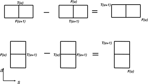
Figure 11: Two equations for the first Bäcklund transformation (BT1) in the $(s,a)$ plane: the variables change within a “brick” consisting of two neighboring squares.

There is a remarkable duality between $T(a,s,u)$ and $F(a,s,u)$ [30, 16]: one can exchange the roles of the functions $T$, $F$ and treat eqs. (3.10) as an over-determined system of linear problems for the function $T$ with coefficients $F$. Their compatibility condition is the same Hirota equation for $F$:

$$F(a,s,u+1)F(a,s,u-1)-F(a,s+1,u)F(a,s-1,u)=F(a+1,s,u)F(a-1,s,u)\,.$$ (3.14)

This can be seen by rewriting (3.10) in yet another equivalent form. Namely, shifting $a\to a+1$ in the first equation and $s\to s-1$ in the second, we represent the two equations in the matrix form

$$\left(\begin{array}[]{cc}F(a\!+\!1,s,u)&F(a,s\!+\!1,u)\\ &\\ F(a,s\!-\!1,u)&-F(a\!-\!1,s,u)\end{array}\right)\left(\begin{array}[]{c}T(a,\,s,\,u\!+\!1)\\ \\ T(a\!+\!1,s\!-\!1,u\!+\!1)\end{array}\right)=F(a,s,u\!+\!1)\left(\begin{array}[]{c}T(a\!+\!1,s,u)\\ \\ F(a,s\!-\!1,u)\end{array}\right)$$ (3.15)

which is to be compared with (3.11). It is obvious that they differ by the substitution $T\leftrightarrow F$ and changing signs of all variables. Therefore, we get the same Hirota equation for $F$. We thus conclude that any solution to the linear problems (3.10), where the $T$-function obeys the Hirota equation, provides an auto-Bäcklund transformation, i.e., a transformation that sends a solution of the nonlinear integrable equation to another solution of the same equation. In what follows we call them simply Bäcklund transformations (BT) and distinguish two types of them.

Let us rewrite the linear problems (3.10) changing the order of the terms and shifting the variables:

$$T(a\!+\!1,s,u)F(a,s,u\!+\!1)-T(a,s,u\!+\!1)F(a\!+\!1,s,u) = T(a\!+\!1,s\!-\!1,u\!+\!1)F(a,s\!+\!1,u),$$

$$T(a,s\!+\!1,u\!+\!1)F(a,s,u)-T(a,s,u)F(a,s\!+\!1,u\!+\!1) = T(a\!+\!1,s,u\!+\!1)F(a\!-\!1,s\!+\!1,u).$$ (3.16)

These equations are graphically represented in Fig. 11 in the $(s,a)$ plane. Given polynomials $T(a,s,u)$ obeying the Hirota equation, we are going to seek for polynomial solutions for $F$.

It is easy to see that equations (3.2) are not compatible if one imposes the boundary conditions for $F(a,s,u)$ and $T(a,s,u)$ of the fat hook type with the same $K$ and $M$. Indeed, applying them in the corner point of the interior boundary, one sees that the boundary values must vanish identically. However, it is straightforward to verify that equations (3.2) are compatible with the boundary conditions of the following two types. The boundary conditions for $F(a,s,u)$ can be either

$$F(a,s,u)=0\quad{\rm if:}\quad\mbox{(i)}\;\;a<0\quad{\rm or}\quad\mbox{(ii)}\;\;s<0\;\;{\rm and}\;\;a\neq 0,\quad{\rm or}\quad\mbox{(iii)}\;\;a>K\!-\!1\;\;{\rm and}\;\;s>M,$$ (3.17)

or

$$F(a,s,u)=0\quad{\rm if:}\quad\mbox{(i)}\;\;a<0\quad{\rm or}\quad\mbox{(ii)}\;\;s<0\;\;{\rm and}\;\;a\neq 0,\quad{\rm or}\quad\mbox{(iii)}\;\;a>K\;\;{\rm and}\;\;s>M+1\,,$$ (3.18)

which are again of the fat hook type but with the shifts $K\to K-1$ or $M\to M+1$.

3.2.1 First Bäcklund transformation

The first Bäcklund transformation (BT1) $T\longrightarrow F$ is given by the linear problems (3.2) with boundary conditions (3.17). Moreover, the linear problems are also compatible with the more specific form of the boundary conditions (3.1), where $K$ is replaced by $K-1$ and $M$ remains the same. To see this, one should check all cases when one of the three terms in the linear equations vanishes, which imposes certain constraints on the boundary functions. The first equation at $s=0$ (the “brick” in position 8 in Fig. 12), with $T(a,0,u)$ as in (3.2), states that $F(a,0,u)$ depends only on $u+a$. Therefore, we can set $F(a,0,u)=Q_{K-1,M}(u+a)$, which at this step is just the notation. Similarly, the second equation at $a=0$ (position 5) implies that $F(0,s,u)$ depends only on $u-s$. At $s=0$ it must equal $Q_{K-1,M}(u)$, therefore, $F(0,s,u)=Q_{K-1,M}(u-s)$.

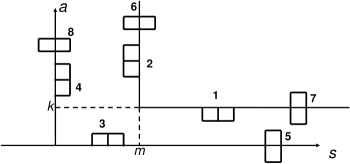
Figure 12: Particular cases of application of the first Bäcklund transformation (BT1) in the form depicted in Fig. 11.

The consistency of the last two boundary conditions in (3.2) follows from a similar analysis at the interior boundaries. Indeed, at $a=K-1,\,\,s>M$ (position 1) the first equation becomes

$$\begin{array}[]{ll}&Q_{K,0}(u+s+K)Q_{0,M}(u-s-K)F(K-1,s,u+1)\\ &\\ =&Q_{K,0}(u+s+K)Q_{0,M}(u-s-K+2)F(K-1,s+1,u)\,.\end{array}$$ (3.19)

This equation fixes the $(u-s)$-dependent factor in $F(K-1,s,u)$ to be $Q_{0,M}(u-s-(K-1))$ while no restrictions on the $(u+s)$-dependent factor emerge. One is free to call it $Q_{K-1,0}(u+s+K-1)$, so that

$$F(K-1,s,u)=Q_{K-1,0}(u+s+K-1)Q_{0,M}(u-s-K+1),\quad M\leq s<\infty,$$ (3.20)

i.e., the boundary condition for $F(a,s,u)$ on the half-line $a=K-1,\,\,M\leq s<\infty$ takes the same form as the 3-rd one from eq.(3.1) for $T(a,s,u)$ on the half-line $a=K,\,\,M\leq s<\infty$ (see Fig. 10). Finally, one can check that the first equation in (3.2) at $s=M$, $a\geq K$ (position 6) is consistent with

$$F(a,M,u)=(-1)^{M(a-K+1)}Q_{K-1,0}(u+a+M)Q_{0,M}(u-a-M),\quad K-1\leq a<\infty,$$ (3.21)

and does not bring any new constraints. The sign factor is not fixed by this argument. To fix it, one should require consistency with the second Bäcklund transformation which we consider in the next subsection.

3.2.2 Second Bäcklund transformation

As is seen from eq. (3.18), the transformations generated by the linear problems (3.2) are not able to move the vertical part of the interior boundary from the right to the left. For our purpose, we need a transformation which would be able to decrease $M$. Using the duality between $T$ and $F$ explained in the end of Sect. 3.2, one can introduce Bäcklund transformations of the required type. The second Bäcklund transformation (BT2) $T\longrightarrow F^{*}$ is obtained from eq.(3.2) by exchanging $T\to F^{*}$ and $F\to T$:

$$F^{*}(a\!+\!1,s,u)T(a,s,u\!+\!1)-F^{*}(a,s,u\!+\!1)T(a\!+\!1,s,u) = F^{*}(a\!+\!1,s\!-\!1,u\!+\!1)T(a,s\!+\!1,u),$$

$$F^{*}(a,s\!+\!1,u\!+\!1)T(a,s,u)-F^{*}(a,s,u)T(a,s\!+\!1,u\!+\!1) = F^{*}(a\!+\!1,s,u\!+\!1)T(a\!-\!1,s\!+\!1,u).$$ (3.22)

These equations are represented graphically in Fig. 13 in the $(s,a)$ plane. As is argued in Sect. 3.2, their compatibility condition is the Hirota equation (3.1) for $T$. If it holds, then any solution $F^{*}$ obeys the same Hirota equation and thus provides an auto-Bäcklund transformation.

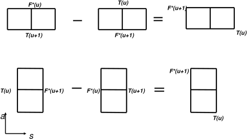
Figure 13: Two equations of the second pair of linear problems in the $(s,a)$ plane.

Given a solution $T(a,s,u)$ with the boundary conditions (3.1), equations (3.2.2) are compatible with the following boundary condition for $F^{*}(a,s,u)$:

$$F^{*}(a,s,u)=0\quad{\rm if:}\quad\mbox{(i)}\;\;a<0\quad{\rm or}\quad\mbox{(ii)}\;\;s<0\;\;{\rm and}\;\;a\neq 0,\quad{\rm or}\quad\mbox{(iii)}\;\;a>K\;\;{\rm and}\;\;s>M-1,$$ (3.23)

which directly follow from (3.18) and differ from those for $T$ (3.2) by the shift $M\to M-1$. Moreover, they are also compatible with the more specific form of the boundary conditions (3.1), where $M$ is replaced by $M-1$ and $K$ remains the same. In complete analogy with BT1, one verifies this by applying BT2 on the exterior boundaries (positions 8 and 5 in Fig. 12) and on the interior ones (positions 7 and 2). In particular, on the half-line $s=M-1,\,K\leq a<\infty$ we have

$$F^{*}(a,M-1,u)=(-1)^{(M-1)(a-K)}Q_{K,0}(u+a+M-1)Q_{0,M-1}(u-a-M+1),\quad K\leq a<\infty,$$ (3.24)

the sign being uniquely fixed from the second equation of (3.2.2) applied in position 2. This means that the boundary condition for $F^{*}(a,s,u)$ on the half-line $s=M-1,\,\,K\leq a<\infty$ takes the same form as the one for $T(a,s,u)$ on the half-line $s=M,\,\,K\leq a<\infty$ (see the 4-th equation in (3.1) and Fig. 14).

Our final goal is to “undress”, using the transformations BT1 and BT2, the original problem by collapsing the region where the Hirota equation acts: $K\to 0,\,\,M\to 0$.

3.3 Hierarchy of Hirota equations and linear problems

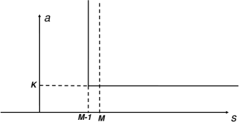
Figure 14: Boundary conditions for the second Bäcklund transformation in the $(s,a)$ plane.

We see now that by applying BT1 or BT2 to a solution to the Hirota equation with the boundary conditions (3.1) we can shift the interior boundaries as $K\to K-1$ or $M\to M-1$ (Fig. 10 and Fig. 14, respectively). In this way we come to the problem for $F(a,s,u)$ or $F^{*}(a,s,u)$ of the same kind as the original problem for $T(a,s,u)$. Repeating these steps several times, we arrive at the hierarchy of the functions $T_{k,m}(a,s,u)$ such that

$$\begin{array}[]{l}T_{K,M}(a,s,u)\equiv T(a,s,u),\\ \\ T_{K-1,M}(a,s,u)\equiv F(a,s,u),\\ \\ T_{K,M-1}(a,s,u)\equiv F^{*}(a,s,u),\quad{\rm etc.},\end{array}$$ (3.25)

all of them satisfying the Hirota equation

$$T_{k,m}(a,s,u+1)T_{k,m}(a,s,u-1)-T_{k,m}(a,s+1,u)T_{k,m}(a,s-1,u)=T_{k,m}(a+1,s,u)T_{k,m}(a-1,s,u)\,,$$ (3.26)

where $k=0,\dots K$ and $m=0,\dots,M$. The boundary conditions are as follows

$$T_{k,m}(a,s,u)=0\quad{\rm if:}\quad\mbox{(i)}\;\;a<0\quad{\rm or}\quad\mbox{(ii)}\;\;s<0\;\;{\rm and}\;\;a\neq 0,\quad{\rm or}\quad\mbox{(iii)}\;\;a>k\;\;{\rm and}\;\;s>m,$$ (3.27)

and

$$T_{k,m}(0,s,u) = Q_{k,m}(u-s),\quad-\infty<s<\infty,$$

$$T_{k,m}(a,0,u) = Q_{k,m}(u+a),\quad 0\leq a<\infty,$$

$$T_{k,m}(k,s,u) = Q_{k,0}(u\!+\!s\!+\!k)\,Q_{0,m}(u\!-\!s\!-\!k),\quad m\leq s<\infty,$$

$$T_{k,m}(a,m,u) = (-1)^{m(a-k)}\,Q_{k,0}(u\!+\!a\!+\!m)\,Q_{0,m}(u\!-\!a\!-\!m),\quad k\leq a<\infty,$$ (3.28)

(see Fig. 9). The function $Q_{K,M}(u)$ is a fixed polynomial of degree $N$ which depends on the choice of the quantum (super) spin chain with the $gl(K|M)$ symmetry. We set $Q_{0,0}(u)=1$ (it corresponds to an empty chain). The other polynomial functions $Q_{k,m}(u)$ will be determined from polynomial solutions to the hierarchy of Hirota equations.

The linear problem (3.2) generates a chain of Bäcklund transformations BT1:

$$\begin{array}[]{c}T_{k,m}(a+1,s,u)T_{k-1,m}(a,s,u+1)-T_{k,m}(a,s,u+1)T_{k-1,m}(a+1,s,u)\\ \\ =\,\,T_{k,m}(a+1,s-1,u+1)T_{k-1,m}(a,s+1,u),\\ \\ T_{k,m}(a,s+1,u+1)T_{k-1,m}(a,s,u)-T_{k,m}(a,s,u)T_{k-1,m}(a,s+1,u+1)\\ \\ =\,\,T_{k,m}(a+1,s,u+1)T_{k-1,m}(a-1,s+1,u),\\ \\ \end{array}$$ (3.29)

($k=1,\dots,K$). The linear problem (3.2.2) generates a chain of Bäcklund transformations BT2:

$$\begin{array}[]{c}T_{k,m-1}(a+1,s,u)T_{k,m}(a,s,u+1)-T_{k,m-1}(a,s,u+1)T_{k,m}(a+1,s,u)\\ \\ =\,\,T_{k,m-1}(a+1,s-1,u+1)T_{k,m}(a,s+1,u),\\ \\ T_{k,m-1}(a,s+1,u+1)T_{k,m}(a,s,u)-T_{k,m-1}(a,s,u)T_{k,m}(a,s+1,u+1)\\ \\ =\,\,T_{k,m-1}(a+1,s,u+1)T_{k,m}(a-1,s+1,u)\end{array}$$ (3.30)

($m=1,\dots,M$). Note that (3.30) differs from (3.29) only by the “direction” of the Bäcklund flow: it is $k\to k-1$ in (3.29) and $m\to m+1$ in (3.30). In the 5D linear space with coordinates $a,s,u,k,m$, the four equations (3.29), (3.30) act in the hyper-planes

$$\begin{array}[]{c}\{m=\mbox{const}\}\,\cap\,\{u+s+a=\mbox{const}\},\\ \\ \{m=\mbox{const}\}\,\cap\,\{u-s-a=\mbox{const}\},\\ \\ \{k=\mbox{const}\}\,\cap\,\{u+s+a=\mbox{const}\},\\ \\ \{k=\mbox{const}\}\,\cap\,\{u-s-a=\mbox{const}\},\end{array}$$

respectively. Thus each of them is actually a dynamical equation in three variables rather than five. It is easy to see that all of them can be transformed to the standard form of the Hirota equation (B2) by linear changes of variables.

The two Bäcklund transformations can be unified in a matrix equation of the type (3.13). Let ${\mathbb{T}}_{k,m}(a,s,u)$ be the antisymmetric matrix from the left hand side in (3.13) at the level $k,m$:

$${\mathbb{T}}_{k,m}(a,s,u)=\left(\begin{array}[]{cccc}0&T_{k,m}(a,s,u\!-\!1)&-T_{k,m}(a,s\!+\!1,u)&T_{k,m}(a\!+\!1,s,u)\\ &&&\\ -T_{k,m}(a,s,u\!-\!1)&0&T_{k,m}(a\!-\!1,s,u)&T_{k,m}(a,s\!-\!1,u)\\ &&&\\ T_{k,m}(a,s\!+\!1,u)&-T_{k,m}(a\!-\!1,s,u)&0&-T_{k,m}(a,s,u\!+\!1)\\ &&&\\ -T_{k,m}(a\!+\!1,s,u)&-T_{k,m}(a,s\!-\!1,u)&T_{k,m}(a,s,u\!+\!1)&0\end{array}\right),$$ (3.31)

then the Bäcklund transformations BT1 and $(\mbox{BT2})^{-1}$ (the transformation inverse to BT2) in the symmetric form are obtained as the first and the second columns of the matrix equation

$${\mathbb{T}}_{k,m}(a,s,u)\left(\begin{array}[]{cc}T_{k\!-\!1,m}(a\!-\!1,\,s,\,u)&T_{k,m\!+\!1}(a\!-\!1,\,s,\,u)\\ &\\ T_{k\!-\!1,m}(a,\,s\!+\!1,\,u)&T_{k,m\!+\!1}(a,\,s\!+\!1,\,u)\\ &\\ T_{k\!-\!1,m}(a,\,s,\,u\!-\!1)&T_{k,m\!+\!1}(a,\,s,\,u\!-\!1)\\ &\\ T_{k\!-\!1,m}(a\!-\!1,s\!+\!1,u\!-\!1)&T_{k,m\!+\!1}(a\!-\!1,s\!+\!1,u\!-\!1)\end{array}\right)=0.$$ (3.32)

The first and the second equations in (3.29), (3.30) are obtained in the second and the first lines of the matrix equation (3.32) respectively. As we have seen above, the rank of the $4\times 4$ matrix ${\mathbb{T}}_{k,m}$ is $2$, so it has two linearly independent zero eigenvectors. Now we see that they correspond to the two independent transformations shifting either $k$ or $m$.

3.4 Bilinear equations for the $T$-functions with different $k$ and $m$

In this subsection we derive additional bilinear equations (3.38)-(3.43) for the functions $T_{k,m}(a,s,u)$ in which both indices $k,m$ undergo shifts by $\pm 1$. They are also of the Hirota type. A special case of them (equation (3.45)) is particularly important. It provides a bilinear relation for the $Q$-functions (the “$QQ$-relation”) which will be also derived in section 4 by other means.

All these additional bilinear relations follow from compatibility of equations (3.29), (3.30) with shifts in $k$ and in $m$. To see this more explicitly, we note that these equations admit a remarkable alternative representation. Namely, it is straightforward to verify that the first equations in (3.29), (3.30) can be identically rewritten as

$$\frac{T_{k-1,m}(a\!+\!1,s,u)}{T_{k-1,m}(a,s\!+\!1,u)}=\left[\frac{T_{k-1,m}(a,s,u\!+\!1)T_{k,m}(a,s\!+\!1,u)}{T_{k-1,m}(a,s\!+\!1,u)T_{k,m}(a,s,u\!+\!1)}-e^{\partial_{u}-\partial_{s}}\right]\frac{T_{k,m}(a\!+\!1,s,u)}{T_{k,m}(a,s\!+\!1,u)}\,,$$ (3.33)

$$\frac{T_{k,m+1}(a\!+\!1,s,u)}{T_{k,m+1}(a,s\!+\!1,u)}=\left[\frac{T_{k,m+1}(a,s,u\!+\!1)T_{k,m}(a,s\!+\!1,u)}{T_{k,m+1}(a,s\!+\!1,u)T_{k,m}(a,s,u\!+\!1)}-e^{\partial_{u}-\partial_{s}}\right]\frac{T_{k,m}(a\!+\!1,s,u)}{T_{k,m}(a,s\!+\!1,u)}\,,$$ (3.34)

while the second equations as

$$\frac{T_{k+1,m}(a,s\!+\!1,u)}{T_{k+1,m}(a\!+\!1,s,u)}=\left[\frac{T_{k+1,m}(a,s,u\!-\!1)T_{k,m}(a\!+\!1,s,u)}{T_{k+1,m}(a\!+\!1,s,u)T_{k,m}(a,s,u\!-\!1)}+e^{-\partial_{u}-\partial_{a}}\right]\frac{T_{k,m}(a,s\!+\!1,u)}{T_{k,m}(a\!+\!1,s,u)}\,,$$ (3.35)

$$\frac{T_{k,m-1}(a,s\!+\!1,u)}{T_{k,m-1}(a\!+\!1,s,u)}=\left[\frac{T_{k,m-1}(a,s,u\!-\!1)T_{k,m}(a\!+\!1,s,u)}{T_{k,m-1}(a\!+\!1,s,u)T_{k,m}(a,s,u\!-\!1)}+e^{-\partial_{u}-\partial_{a}}\right]\frac{T_{k,m}(a,s\!+\!1,u)}{T_{k,m}(a\!+\!1,s,u)}\,.$$ (3.36)

In this form they appear as linear problems for the difference operators in the brackets together with particular solutions. One can notice that they again look like auxiliary linear problems for the Hirota equation but for a different choice of the variables. For example, equations (3.33), (3.34) should be compared with eq. (B1) from Appendix B, where we identify $\tau$ with $T$ and choose the variables as $p_{1}=-k$, $p_{2}=m$, $p_{3}=\frac{1}{2}(u-s)$ (note that the variables $a$ and $\frac{1}{2}(u+s)$ are kept constant in the $T$-functions entering the difference operator in (3.33), (3.34)). We see that the two equations coincide with the two corresponding linear problems from (B1) (with $\lambda_{1}=-\lambda_{2}=1$), with

$$\psi_{k,m}(a,s,u)=\frac{T_{k,m}(a\!+\!1,s,u)}{T_{k,m}(a,s\!+\!1,u)}$$

being their common solution. Because they hold for any $k,m$, the function $\psi_{k-1,m+1}(a,s,u)$ can be represented in two different ways as follows:

$$\left[\frac{T_{k-1,m+1}(a,s,u\!+\!1)T_{k-1,m}(a,s\!+\!1,u)}{T_{k-1,m+1}(a,s\!+\!1,u)T_{k-1,m}(a,s,u\!+\!1)}-e^{\partial_{u}-\partial_{s}}\right]\left[\frac{T_{k-1,m}(a,s,u\!+\!1)T_{k,m}(a,s\!+\!1,u)}{T_{k-1,m}(a,s\!+\!1,u)T_{k,m}(a,s,u\!+\!1)}-e^{\partial_{u}-\partial_{s}}\right]\psi_{k,m}$$

$$=\,\,\,\left[\frac{T_{k-1,m+1}(a,s,u\!+\!1)T_{k,m+1}(a,s\!+\!1,u)}{T_{k-1,m+1}(a,s\!+\!1,u)T_{k,m+1}(a,s,u\!+\!1)}-e^{\partial_{u}-\partial_{s}}\right]\left[\frac{T_{k,m+1}(a,s,u\!+\!1)T_{k,m}(a,s\!+\!1,u)}{T_{k,m+1}(a,s\!+\!1,u)T_{k,m}(a,s,u\!+\!1)}-e^{\partial_{u}-\partial_{s}}\right]\psi_{k,m}\,.$$

Opening the brackets, one finds that the terms multiplied by $\psi_{k,m}(a,s,u)$ and $\psi_{k,m}(a,s\!-\!2,u\!+\!2)$ cancel automatically while the terms proportional to $\psi_{k,m}(a,s\!-\!1,u\!+\!1)$ give a non-trivial relation connecting the $T$-functions with different $k$ and $m$. It has the form

$$\begin{array}[]{c}T_{k,m}(a,s\!+\!1,u)T_{k+1,m+1}(a,s,u\!+\!1)-T_{k,m}(a,s,u\!+\!1)T_{k+1,m+1}(a,s\!+\!1,u)\\ \\ =\,\,\,f_{k,m}(a,u\!+\!s)\,T_{k+1,m}(a,s,u\!+\!1)T_{k,m+1}(a,s\!+\!1,u)\,,\end{array}$$ (3.37)

where $f_{k,m}(a,u\!+\!s)$ is an arbitrary function of $k,m$ and $a,\,u+s$. Comparing it with a similar equation obtained in the same way from the other pair of linear problems (3.35), (3.36), one can see that it actually depends on the combination $u+s-a$ as well as on $k,m$ (see Appendix C for details). To fix it, we take $s=m$, so the first term of the equation vanishes (at $a\geq k+1$), and use boundary conditions (3.3). This fixes the function $f_{k,m}$ to be $1$.

Clearly, eq. (3.37) (with $f_{k,m}(a,u\!+\!s)=1$) is the Hirota equation of the form (B2) in the variables $-k$, $m$ and $\frac{1}{2}(u-s)$. The Hirota equation implies the compatibility of the linear problems, i.e., the discrete zero curvature condition for the difference operators in (3.33), (3.34) holds true. In our situation, it appears to be equivalent to the “weak form” of this condition, i.e., with the operators being applied to a particular solution of the linear problems. In other words, the compatibility of the linear problems (which in general means existence of a continuous family of common solutions) follows, in our case, from the existence of just one common solution (cf. [44]).

There are other equations of the same type. It is convenient to write them all as the following chain of equalities:

$$1 = \frac{T_{k,m}(a,s+1,u)T_{k+1,m+1}(a,s,u+1)-T_{k,m}(a,s,u+1)T_{k+1,m+1}(a,s+1,u)}{T_{k,m+1}(a,s+1,u)T_{k+1,m}(a,s,u+1)}$$ (3.38)

$$= \frac{T_{k,m}(a-1,s,u)T_{k+1,m+1}(a,s,u+1)-T_{k,m}(a,s,u+1)T_{k+1,m+1}(a-1,s,u)}{T_{k,m+1}(a-1,s,u)T_{k+1,m}(a,s,u+1)}$$ (3.39)

$$= \frac{T_{k,m}(a-1,s,u)T_{k+1,m+1}(a,s-1,u)-T_{k,m}(a,s-1,u)T_{k+1,m+1}(a-1,s,u)}{T_{k,m+1}(a-1,s,u)T_{k+1,m}(a,s-1,u)}\,.$$ (3.40)

These equations have the same structure. In each equation, one of the variables $a,s,u$ enters as a parameter. More precisely, they act in the hyper-planes

$$\begin{array}[]{c}\{a=\mbox{const}\}\,\cap\,\{u+s=\mbox{const}\},\\ \\ \{s=\mbox{const}\}\,\cap\,\{u-a=\mbox{const}\},\\ \\ \{u=\mbox{const}\}\,\cap\,\{a+s=\mbox{const}\},\\ \\ \end{array}$$

respectively. The first equality in this chain is already proved. The proof of the other two is straightforward: one should pass to common denominator, to group together similar terms and to use equations (3.32). In fact this chain can be continued by three more equations of a similar but different structure:

$$1 = \frac{T_{k,m}(a,s-1,u)T_{k+1,m+1}(a,s,u+1)-T_{k,m}(a,s,u+1)T_{k+1,m+1}(a,s-1,u)}{T_{k,m+1}(a-1,s,u)T_{k+1,m}(a+1,s-1,u+1)}$$ (3.41)

$$= \frac{T_{k,m}(a,s,u+1)T_{k+1,m+1}(a+1,s,u)-T_{k,m}(a+1,s,u)T_{k+1,m+1}(a,s,u+1)}{T_{k,m+1}(a,s+1,u)T_{k+1,m}(a+1,s-1,u+1)}$$ (3.42)

$$= \frac{T_{k,m}(a,s-1,u)T_{k+1,m+1}(a+1,s,u)-T_{k,m}(a+1,s,u)T_{k+1,m+1}(a,s-1,u)}{T_{k,m+1}(a,s,u-1)T_{k+1,m}(a+1,s-1,u+1)}\,.$$ (3.43)

They are proved in the same manner. There is no need to prove the first equality separately since one can just continue the chain of equations (3.38)-(3.40) proving that (3.40) is equal to (3.41). Other forms of these equations and more details can be found in Appendix C. Equations (3.41)-(3.43) act in the hyper-planes

$$\begin{array}[]{c}\{a-k+m=\mbox{const}\}\,\cap\,\{u-s-a=\mbox{const}\},\\ \\ \{s+k-m=\mbox{const}\}\,\cap\,\{u+s+a=\mbox{const}\},\\ \\ \{u-k+m=\mbox{const}\}\,\cap\,\{u+s-a=\mbox{const}\},\\ \\ \end{array}$$

respectively. Therefore, equations (3.38)-(3.40) and (3.41)-(3.43) are actually equations in three variables rather than five. They can be transformed to the standard form of the Hirota equation (B2) by linear changes of variables.

We note that equations (3.38)-(3.40) can be written in the following concise form:

$$\left(e^{\partial_{p}}-e^{\partial_{q}}\right)\frac{T_{k+1,m+1}}{T_{km}}\,=\,\left(e^{\partial_{p}}\frac{T_{k+1,m}}{T_{km}}\right)\left(e^{\partial_{q}}\frac{T_{k,m+1}}{T_{km}}\right)\,.$$ (3.44)

Here $T_{k,m}\equiv T_{k,m}(a,u,s)$ and $(p,q)$ stands for any one of the pairs $(u,s)$, $(u,-a)$ and $(a,s)$.

Restricting the bilinear equations to the boundaries of the fat hook domain, one obtains new equations which include the $Q$-functions. For example, setting $a=0$ in eq. (3.37) (or eq. (3.38)) and using (3.3), we get the $QQ$-relation mentioned in the Introduction:

$$Q_{k,m}(u)Q_{k+1,m+1}(u+2)-Q_{k,m}(u+2)Q_{k+1,m+1}(u)=Q_{k,m+1}(u)Q_{k+1,m}(u+2)\,.$$ (3.45)

In the next section, it will be derived by other means. Another new relation, which is of a mixed ($TQ$ and $QQ$) type, is the particular case of eq. (3.43) at $a=0,s=1$:

$$T_{k+1,m+1}(1,1,u)Q_{k,m}(u)-T_{k,m}(1,1,u)Q_{k+1,m+1}(u)=Q_{k,m+1}(u-2)Q_{k+1,m}(u+2)\,.$$ (3.46)

4 $TQ$- and $QQ$-relations

In this section we partially solve the “undressing” problem for the hierarchy of the $T$-functions $T_{k,m}(a,s,u)$ and derive the generalized Baxter equations ($TQ$-relations) which express $T(1,s,u)$, $T(a,1,u)$ through the Baxter functions $Q_{k,m}(u)$. This is done by constructing an operator generating series for the $T$-functions and factorizing it into an ordered product of first order difference operators, with coefficients being ratios of the $Q$-functions. These operators obey a discrete zero curvature condition which leads to a bilinear relation for the functions $Q_{k,m}$ with different values of $k,m$ (the $QQ$-relation).

4.1 Operator generating series and generalized Baxter relations

We start by introducing the following difference operators of infinite order:

$$\hat{W}_{k,m}(u) = \sum_{s=0}^{\infty}\frac{T_{k,m}(1,s,u\!+\!s\!+\!1)}{Q_{k,m}(u)}\,e^{2s\partial_{u}},$$

$$\check{W}_{k,m}(u) = \sum_{a=0}^{\infty}(-1)^{a}e^{2a\partial_{u}}\,\frac{T_{k,m}(a,1,u\!-\!a\!+\!1)}{Q_{k,m}(u+2)}$$ (4.1)

which represent operator generating series for the transfer matrices corresponding to one-row or one-column Young diagrams. The denominators are introduced for the proper normalization. Let us show that the difference operators

$$\hat{U}_{k,m}(u) = \frac{Q_{k+1,m}(u)\,Q_{k,m}(u\!+\!2)}{Q_{k+1,m}(u\!+\!2)\,Q_{k,m}(u)}\,-\,\,e^{2\partial_{u}},$$

$$\hat{V}_{k,m}(u) = \frac{Q_{k,m}(u)\,Q_{k,m+1}(u\!+\!2)}{Q_{k,m}(u\!+\!2)\,Q_{k,m+1}(u)}\,-\,\,e^{2\partial_{u}}.$$ (4.2)

shift the level indices $k,m$ of the $\hat{W}_{k,m}(u)$ and $\check{W}_{k,m}(u)$. Namely, we are going to prove the following operator relations:

$$\hat{W}_{k,m}(u) = \hat{U}_{k,m}(u)\hat{W}_{k+1,m}(u),$$

$$\hat{W}_{k,m+1}(u) = \hat{V}_{k,m}(u)\,\hat{W}_{k,m}(u),$$ (4.3)

$$\check{W}_{k\!+\!1,m}(u) = \check{W}_{k,m}(u)\,\hat{U}_{k,m}(u),$$

$$\check{W}_{k,m}(u) = \check{W}_{k,m\!+\!1}(u)\,\hat{V}_{k,m}(u).$$ (4.4)

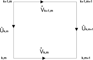
Figure 15: The discrete zero curvature condition $\hat{U}_{k,m+1}\hat{V}_{k+1,m}=\hat{V}_{k,m}\hat{U}_{k,m}$.

To prove the first equation in (4.1), we write

$$\hat{W}_{k-1}(u)+e^{2\partial_{u}}\hat{W}_{k}(u)=\hat{W}_{k-1}(u)+\hat{W}_{k}(u+2)e^{2\partial_{u}}$$

$$=\,\,\,\,\frac{T_{k-1}(1,0,u+1)}{Q_{k-1}(u)}+\sum_{s=1}^{\infty}\left[\frac{T_{k-1}(1,s,u\!+\!s\!+\!1)}{Q_{k-1}(u)}+\frac{T_{k}(1,s\!-\!1,u\!+\!s\!+\!2)}{Q_{k}(u+2)}\,\right]e^{2s\partial_{u}}\,.$$ (4.5)

(Here and below in the proof we omit the second index $m$ since it is the same everywhere.) To transform the expression in the square brackets, we use the first equation of the BT1 at $a=0$ (position 3 in Fig. 12):

$$T_{k}(1,s,u)Q_{k-1}(u\!-\!s\!+\!1)-T_{k-1}(1,s,u)Q_{k}(u\!-\!s\!+\!1)=T_{k}(1,s\!-\!1,u\!+\!1)Q_{k-1}(u\!-\!s\!-\!1).$$ (4.6)

Shifting it $u\to u+s+1$ and dividing both sides by $Q_{k}(u+2)Q_{k-1}(u)$, we obtain

$$\frac{T_{k}(1,s,u+s+1)Q_{k-1}(u+2)}{Q_{k}(u+2)Q_{k-1}(u)}\,-\,\frac{T_{k-1}(1,s,u+s+1)}{Q_{k-1}(u)}\,=\,\frac{T_{k}(1,s-1,u+s+2)}{Q_{k}(u+2)}\,.$$

Using this, we rewrite the term in the square brackets under the sum in eq.(4.1) as

$$\frac{Q_{k}(u)\,Q_{k-1}(u\!+\!2)}{Q_{k}(u\!+\!2)\,Q_{k-1}(u)}\,\,\frac{T_{k}(1,s,u+s+1)}{Q_{k}(u)}$$

and continue the equality (4.1):

$$\hat{W}_{k-1}(u)+e^{2\partial_{u}}\hat{W}_{k}(u) = \frac{T_{k-1}(1,0,u+1)}{Q_{k-1}(u)}+\frac{Q_{k}(u)\,Q_{k-1}(u\!+\!2)}{Q_{k}(u\!+\!2)\,Q_{k-1}(u)}\sum_{s=1}^{\infty}\frac{T_{k}(1,s,u\!+\!s\!+\!1)}{Q_{k}(u)}\,e^{2s\partial_{u}}$$ (4.7)

$$= \frac{Q_{k}(u)\,Q_{k-1}(u\!+\!2)}{Q_{k}(u\!+\!2)\,Q_{k-1}(u)}\sum_{s=0}^{\infty}\frac{T_{k}(1,s,u+s+1)}{Q_{k}(u)}\,e^{2s\partial_{u}}.$$

In the last step we have noticed that the $s=0$ term of the sum multiplied by the ratio of $Q$’s is just equal to $T_{k-1}(1,0,u+1)/Q_{k-1}(u)$. The sum in the r.h.s. is $\hat{W}_{k}(u)$, so the first equality in (4.1) is proved. The proof of the three other equations in (4.1-4.1) is completely similar.

Combining equations (4.1),(4.1), we see that

$$\check{W}_{k-1,m}(u)\hat{W}_{k-1,m}(u)=\check{W}_{k,m}(u)\hat{W}_{k,m}(u)=\check{W}_{k,m+1}(u)\hat{W}_{k,m+1}(u)\,,$$

i.e., the operator $\check{W}_{k,m}(u)\hat{W}_{k,m}(u)$ does not depend on $k,m$. Note that $\hat{W}_{0,0}(u)=\check{W}_{0,0}(u)=1$ as operators, since all the terms in (4.1) are zero except the first one, which is $1$ thanks to the “boundary conditions” $T_{0,0}(1,0,u+1)=Q_{0,0}(u+2)=1,T_{0,0}(0,1,u+1)=Q_{0,0}(u)=1$. Therefore, we conclude that the operators $\hat{W}_{k,m}$ and $\check{W}_{k,m}$ are mutually inverse:

$$\check{W}_{k,m}(u)\hat{W}_{k,m}(u)=1.$$ (4.8)

In addition, applying equations (4.1), (4.1) many times, we arrive at the following operator relations:

$$\begin{array}[]{lll}\hat{W}_{k,m}&=&\hat{U}^{-1}_{k-1,m}\dots\hat{U}^{-1}_{0,m}\,\hat{V}_{0,m-1}\dots\hat{V}_{0,0},\\ &&\\ \check{W}_{k,m}&=&\hat{V}^{-1}_{0,0}\dots\hat{V}^{-1}_{0,m-1}\,\hat{U}_{0,m}\dots\hat{U}_{k-1,m},\end{array}$$ (4.9)

where we have skipped $u$ since it is the same everywhere. Taking equations (4.1), (4.9) at $k=K$, $m=M$, we obtain the “non-commutative generating functions” for the transfer matrices in the basic representations $(s^{1})$ or $(1^{a})$:

$$\sum_{s=0}^{\infty}\frac{T_{K,M}(1,s,u+s+1)}{Q_{K,M}(u)}\,e^{2s\partial_{u}} = \hat{U}^{-1}_{K-1,M}(u)\dots\hat{U}^{-1}_{0,M}(u)\,\hat{V}_{0,M-1}(u)\dots\hat{V}_{0,0}(u),$$

$$\sum_{a=0}^{\infty}(-1)^{a}\frac{T_{K,M}(a,1,u+a+1)}{Q_{K,M}(u+2a+2)}\,e^{2a\partial_{u}} = \hat{V}^{-1}_{0,0}(u)\dots\hat{V}^{-1}_{0,M-1}(u)\,\hat{U}_{0,M}(u)\dots\hat{U}_{K-1,M}(u).$$ (4.10)

Expanding the right hand sides in powers of $e^{2\partial_{u}}$ and comparing the coefficients, one obtains a set of generalized Baxter relations between $T$’s and $Q$’s. In principle, these formulas solve our original problem: they give solutions to the Hirota equation in terms of the $Q$-functions representing the boundary conditions at each level $k,m$.

4.2 Zero curvature condition and $QQ$-relation

The $Q$-functions are polynomials whose roots obey the Bethe equations. Contrary to the case of bosonic $gl(K)$ algebras, the Bethe equations for superalgebras admit many different forms. They correspond to all possible “undressing paths” in the $(k,m)$ plane. Their equivalence can be established by means of certain “duality transformations” [14].

Here we suggest an easy transparent argument to derive all these systems of Bethe equations and the corresponding duality transformations. Namely, we are going to show that the functions $Q_{k,m}(u)$ obey their own Hirota equation. Given an undressing path, it immediately produces the chain of Bethe equations. The duality transformation is nothing else than the discrete zero curvature condition for the operators (4.1) on the $k,m$ lattice.

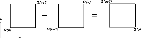
Figure 16: The Hirota equation for the Baxter functions $Q_{k,m}(u)$ in the $(k,m)$ plane.

Equations (4.1) imply $\hat{W}_{k-1,m+1}=\hat{U}_{k-1,m+1}\hat{V}_{k,m}\hat{W}_{k,m}=\hat{V}_{k-1,m}\hat{U}_{k-1,m}\hat{W}_{k,m}$ which gives the discrete zero curvature condition

$$\hat{U}_{k,m+1}\hat{V}_{k+1,m}=\hat{V}_{k,m}\hat{U}_{k,m}.$$ (4.11)

We remark that it looks a bit non-symmetric because $\hat{V}$ shifts $m$ by $+1$ while $\hat{U}$ shifts $k$ by $-1$. Being written through $\hat{U}^{-1}$ and $\hat{V}$, the zero curvature condition acquires the standard symmetric form

$$\hat{U}_{k,m+1}^{-1}\hat{V}_{k,m}=\hat{V}_{k+1,m}\hat{U}_{k,m}^{-1}.$$ (4.12)

As a consequence of it, the following bilinear relation for the $Q^{\prime}s$ is valid:

$$Q_{k,m}(u)Q_{k+1,m+1}(u+2)-Q_{k+1,m+1}(u)Q_{k,m}(u+2)=Q_{k,m+1}(u)Q_{k+1,m}(u+2).$$ (4.13)

It was already derived in section 3.4 as a particular case of more general “$TT$-relations” (3.38), (3.39) (see (3.45)). This is the Hirota equation in “chiral” variables (see Appendix B). Strictly speaking, the zero curvature condition (4.11) implies eq.(4.13) up to an additional factor in the r.h.s. depending on $k,m$ which remains unfixed by this argument. However, this factor can always be eliminated by an appropriate normalization of $Q_{k,m}(u)$’s:

$$Q_{k,m}(u)=A_{k,m}\prod_{j=1}^{J_{k,m}}\left(u-u_{j}^{(k,m)}\right)\,,$$ (4.14)

i.e., by choosing the coefficients $A_{k,m}$. Moreover, the result of section 3.4 shows that the boundary conditions (3.3) already imply the normalization in which the $QQ$-relation has the form (4.13) (see the argument right after eq. (3.37)).

The zero curvature condition allows us to represent equations (4.1) in a more general form. Given an arbitrary zigzag path $\gamma_{K,M}$ from $(K,M)$ to $(0,0)$, the r.h.s. of these equations becomes the ordered product of the shift operators along it (see Fig. 17):

$$\begin{array}[]{rcl}\displaystyle{\sum_{s=0}^{\infty}\,\frac{T_{K,M}(1,s,u+s+1)}{Q_{K,M}(u)}\,e^{2s\partial_{u}}}&=&\displaystyle{\prod\limits_{({\bf x,n})\in\gamma_{K,M}}^{\longleftarrow}\hat{V}_{({\bf x,n})}(u)}\,,\\ &&\\ \displaystyle{\sum_{a=0}^{\infty}(-1)^{a}\frac{T_{K,M}(a,1,u+a+1)}{Q_{K,M}(u+2a+2)}\,e^{2a\partial_{u}}}&=&\displaystyle{\prod\limits_{({\bf x,n})\in\gamma_{K,M}}^{\longrightarrow}\hat{V}^{-1}_{({\bf x,n})}(u)}\,.\end{array}$$ (4.15)

Here we use the natural notation: ${\bf x}$ is the vector on the lattice with coordinates $(k,m)$ ($k$ is the vertical coordinate and $m$ is the horizontal coordinate!), ${\bf n}=(-1,0)$ or $(0,-1)$ is the unit vector looking along the next step of the path. In other words, $({\bf x},{\bf n})$ is the (oriented) edge of the path from $(K,M)$ to $(0,0)$ starting at the point ${\bf x}$ and looking in the direction ${\bf n}$. In the first equation, the shift operators are ordered from the last edge of the path (ending at the origin) to the first one while in the second equation the order is opposite. In fact the zero curvature condition implies that equations (4.15) remain true for any path leading from $(K,M)$ to the origin provided the shift operators are chosen as follows:

$$\begin{array}[]{llll}\hat{V}_{({\bf x,n})}(u)&=&\hat{U}_{k-1,m}^{-1}(u),&{\bf n}=(-1,0),\\ &&&\\ \hat{V}_{({\bf x,n})}(u)&=&\hat{U}_{k,m}(u),&{\bf n}=(1,0),\\ &&&\\ \hat{V}_{({\bf x,n})}(u)&=&\hat{V}_{k,m}^{-1}(u),&{\bf n}=(0,1),\\ &&&\\ \hat{V}_{({\bf x,n})}(u)&=&\hat{V}_{k,m-1}(u),&{\bf n}=(0,-1).\end{array}$$ (4.16)

Some simple examples of equations (4.15) are given in Section 8.

5 Bethe equations

The bilinear $QQ$-relation (4.13) obtained in the previous section (see also section 3.4 for an alternative derivation) gives the easiest and the most transparent way to derive different systems of Bethe equations and to prove their equaivalence. In a similar way, the generalized $TT$-relations (3.38)-(3.40) can be used to derive a new system of Bethe-like equations for roots of the polynomials $T_{k,m}(a,s,u)$.

5.1 Bethe equations for roots of $Q$’s

To derive the system of equations for zeros of the polynomials $Q_{k,m}$ (4.14), we put $u$ in the Hirota equation (4.13) successively equal to $u_{j}^{(k,m)}$, $u_{j}^{(k+1,m+1)}\!-\!2$, $u_{j}^{(k,m)}\!-\!2$, $u_{j}^{(k+1,m+1)}$, $u_{j}^{(k,m+1)}$ and $u_{j}^{(k+1,m)}\!-\!2$, each corresponding to a zero of one of the six $Q$-functions in the equation. After proper shifts of $k$ and $m$ such that the arguments of the $Q$-functions become $u_{j}^{(k,m)}$ and $u_{j}^{(k,m)}\pm 2$, we get the relations

$$\begin{array}[]{rcll}-\,Q_{k,m}\left(u_{j}^{(k,m)}+2\right)Q_{k+1,m+1}\left(u_{j}^{(k,m)}\right)&=&Q_{k,m+1}\left(u_{j}^{(k,m)}\right)Q_{k+1,m}\left(u_{j}^{(k,m)}+2\right)&\quad\quad({\rm a})\\ &&&\\ -\,Q_{k,m}\left(u_{j}^{(k,m)}-2\right)Q_{k-1,m-1}\left(u_{j}^{(k,m)}\right)&=&Q_{k,m-1}\left(u_{j}^{(k,m)}\right)Q_{k-1,m}\left(u_{j}^{(k,m)}-2\right)&\quad\quad({\rm b})\\ &&&\\ Q_{k,m}\left(u_{j}^{(k,m)}-2\right)Q_{k+1,m+1}\left(u_{j}^{(k,m)}\right)&=&Q_{k+1,m}\left(u_{j}^{(k,m)}\right)Q_{k,m+1}\left(u_{j}^{(k,m)}-2\right)&\quad\quad({\rm c})\\ &&&\\ Q_{k,m}\left(u_{j}^{(k,m)}+2\right)Q_{k-1,m-1}\left(u_{j}^{(k,m)}\right)&=&Q_{k-1,m}\left(u_{j}^{(k,m)}\right)Q_{k,m-1}\left(u_{j}^{(k,m)}+2\right)&\quad\quad({\rm d})\\ &&&\\ Q_{k,m-1}\left(u_{j}^{(k,m)}\right)Q_{k+1,m}\left(u_{j}^{(k,m)}+2\right)&=&Q_{k,m-1}\left(u_{j}^{(k,m)}+2\right)Q_{k+1,m}\left(u_{j}^{(k,m)}\right)&\quad\quad({\rm e})\\ &&&\\ Q_{k,m+1}\left(u_{j}^{(k,m)}\right)Q_{k-1,m}\left(u_{j}^{(k,m)}-2\right)&=&Q_{k,m+1}\left(u_{j}^{(k,m)}-2\right)Q_{k-1,m}\left(u_{j}^{(k,m)}\right)&\quad\quad({\rm f})\,.\end{array}$$ (5.1)

Here $1\leq k\leq K-1$, $1\leq m\leq M-1$ and $j$ runs from $1$ to $J_{k,m}$. This is the (over)complete set of Bethe equations for our problem. Their consistency is guaranteed by the Hirota equation (4.13). To convert them into a more familiar form, let us divide eq. (a) by eq. (c) and eq. (b) by eq. (d). Using also eqs. (e) and (f), it is easy to rewrite the system in the form where each group of equations contains the $Q$-functions at three neighboring sites. In this way we obtain the following sets of equations:

$$\begin{array}[]{lll}\begin{CD}\bullet\\ @V{}V{}V\\ \bullet\\ @V{}V{}V\\ \bullet\end{CD}&\phantom{aaaaa}&\displaystyle{\frac{Q_{k-1,m}\left(u_{j}^{(k,m)}\right)Q_{k,m}\left(u_{j}^{(k,m)}-2\right)Q_{k+1,m}\left(u_{j}^{(k,m)}+2\right)}{Q_{k-1,m}\left(u_{j}^{(k,m)}-2\right)Q_{k,m}\left(u_{j}^{(k,m)}+2\right)Q_{k+1,m}\left(u_{j}^{(k,m)}\right)}=\,-\,1}\,,\end{array}$$ (5.2)

$$\begin{array}[]{lll}\begin{CD}\bullet @<{}<{}<\bullet @<{}<{}<\bullet\end{CD}&\phantom{aa}&\displaystyle{\frac{Q_{k,m+1}\left(u_{j}^{(k,m)}\right)Q_{k,m}\left(u_{j}^{(k,m)}-2\right)Q_{k,m-1}\left(u_{j}^{(k,m)}+2\right)}{Q_{k,m+1}\left(u_{j}^{(k,m)}-2\right)Q_{k,m}\left(u_{j}^{(k,m)}+2\right)Q_{k,m-1}\left(u_{j}^{(k,m)}\right)}=\,-\,1}\,,\end{array}$$ (5.3)

$$\begin{array}[]{lll}\begin{CD}\bullet\\ @V{}V{}V\\ \bullet @<{}<{}<\bullet\end{CD}&\phantom{aaaaaaaaaaaaaaaaaaaaa}&\displaystyle{\frac{Q_{k+1,m}\left(u_{j}^{(k,m)}\right)Q_{k,m-1}\left(u_{j}^{(k,m)}+2\right)}{Q_{k+1,m}\left(u_{j}^{(k,m)}+2\right)Q_{k,m-1}\left(u_{j}^{(k,m)}\right)}=\,1}\,,\end{array}$$ (5.4)

$$\begin{array}[]{lll}\begin{CD}\bullet @<{}<{}<\bullet\\ @V{}V{}V\\ \bullet\end{CD}&\phantom{aaaaaaaaaaaaaaaaaaaaa}&\displaystyle{\frac{Q_{k,m+1}\left(u_{j}^{(k,m)}\right)Q_{k-1,m}\left(u_{j}^{(k,m)}-2\right)}{Q_{k,m+1}\left(u_{j}^{(k,m)}-2\right)Q_{k-1,m}\left(u_{j}^{(k,m)}\right)}=\,1}\,.\end{array}$$ (5.5)

These equations are valid at any point of the $(k,m)$ lattice and do not depend on the choice of the undressing zigzag path. The figures show the sites of the $(k,m)$ lattice ($k$ and $m$ are the vertical and horizontal coordinates respectively) which are connected by the corresponding Bethe equation. The point $(k,m)$ is the one between the other two. The edges of the $(k,m)$ lattice are represented by the arrows which show the directions of the transformations BT1 and BT2. For completeness, we also present here two other equations derived from (5.1):

$$\begin{array}[]{lll}\begin{CD}\bullet\\ @V{}V{}V\\ \bullet @<{}<{}<\bullet\end{CD}&\phantom{aaa}&\displaystyle{\frac{Q_{k,m+1}\left(u_{j}^{(k,m)}\right)Q_{k,m}\left(u_{j}^{(k,m)}-2\right)Q_{k+1,m}\left(u_{j}^{(k,m)}+2\right)}{Q_{k,m+1}\left(u_{j}^{(k,m)}-2\right)Q_{k,m}\left(u_{j}^{(k,m)}+2\right)Q_{k+1,m}\left(u_{j}^{(k,m)}\right)}=\,-\,1}\,,\end{array}$$ (5.6)

$$\begin{array}[]{lll}\begin{CD}\bullet @<{}<{}<\bullet\\ @V{}V{}V\\ \bullet\end{CD}&\phantom{aaa}&\displaystyle{\frac{Q_{k-1,m}\left(u_{j}^{(k,m)}\right)Q_{k,m}\left(u_{j}^{(k,m)}-2\right)Q_{k,m-1}\left(u_{j}^{(k,m)}+2\right)}{Q_{k-1,m}\left(u_{j}^{(k,m)}-2\right)Q_{k,m}\left(u_{j}^{(k,m)}+2\right)Q_{k,m-1}\left(u_{j}^{(k,m)}\right)}=\,-\,1}\,,\end{array}$$ (5.7)

It is clear from the figures that these patterns are forbidden for a zigzag path.

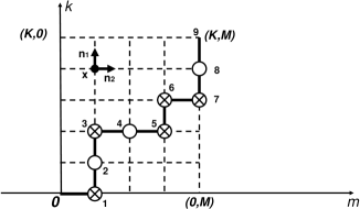
Figure 17: The “undressing” procedure by means of BT1 and BT2 in the $(s,a)$ plane along an arbitrary zigzag path $\gamma_{K,M}$. This path defines the Cartan matrix which characterizes the basis of generators of the Cartan subalgebra.

Let us show how to reduce this 2D array of Bethe equations to a chain. Suppose one fixes a particular zigzag path $\gamma_{K,M}$ from $(K,M)$ to $(0,0)$. Then, for each vertex of the path (except for the first and the last ones), one writes the Bethe equations according to the configuration of the path around the vertex. Let us enumerate vertices of the path by numbers from $0$ to $K+M$ so that the point $(k,m)\in\gamma_{K,M}$ acquires the number $k+m$. Set

$$Q_{k,m}(u)\equiv Q_{k+m}(u)=A_{k+m}\prod_{j=1}^{J_{k+m}}(u-u_{j}^{(k+m)})\,,\quad\quad(k,m)\in\gamma_{K,M}\,.$$

Let us also enumerate edges of the path by numbers from $1$ to $K+M$ so that the edge joining the $(n-1)$-th and the $n$-th vertex acquires the number $n$. (Note that in the course of undressing one passes these edges in the inverse order.) To the $n$-th edge of the path (oriented according to the direction of the undressing, i.e., either from the north to the south or from the east to the west) we assign the sign factor according to the rule:

$$p_{n}=\left\{\begin{array}[]{l}+1\quad\mbox{if the $n$-th edge looks to the south}\\ \\ -1\quad\mbox{if the $n$-th edge looks to the west}\end{array}\right.$$

Then the system of the Bethe equations along the path can be written as follows:

$$\frac{Q_{n+1}\left(u_{j}^{(n)}+2p_{n+1}\right)Q_{n}\left(u_{j}^{(n)}-2p_{n+1}\right)Q_{n-1}\left(u_{j}^{(n)}\right)}{Q_{n+1}\left(u_{j}^{(n)}\right)Q_{n}\left(u_{j}^{(n)}+2p_{n}\right)Q_{n-1}\left(u_{j}^{(n)}-2p_{n}\right)}\,=\,(-1)^{\frac{1+p_{n}p_{n+1}}{2}},$$ (5.8)

where $n$ runs from $1$ to $K+M-1$. The boundary conditions are $Q_{0}(u)=1$, $Q_{K+M}(u)=\phi(u)$. Any chain of Bethe equations includes $K+M-1$ equations for the roots of $K+M-1$ polynomials $Q_{k,m}(u)$ picked along a path as in Fig. 17. All the other $[(K+1)(M+1)-2]-(K+M-1)=KM$ $Q$-functions inside the $K\times M$ rectangle can be expressed through them by iterations of the Hirota equation (4.13).

This form of the Bethe equations agrees with the general one suggested in [3]. To see this, let us redefine the $Q$-functions by the shift of the spectral parameter:

$$Q_{k,m}(u)=\check{Q}_{k+m}\left(u-k+m\right)\,,$$ (5.9)

which is equivalent to

$$Q_{n}(u)=\check{Q}_{n}\left(u-\sum_{\alpha=1}^{n}p_{\alpha}\right)\,.$$ (5.10)

In terms of the roots

$$\check{u}_{j}^{(n)}=u_{j}^{(n)}-\sum_{\alpha=1}^{n}p_{\alpha}\,.$$ (5.11)

of the polynomial $\check{Q}_{n}(u)$ the system of Bethe equations (5.8) acquires a concise form

$$\prod_{b=1}^{K+M}\frac{\check{Q}_{b}\left(\check{u}_{j}^{(a)}-K_{ab}\right)}{\check{Q}_{b}\left(\check{u}_{j}^{(a)}+K_{ab}\right)}=(-1)^{\frac{K_{aa}}{2}}\,,\quad\quad a=1,\ldots,K+M-1\,,$$ (5.12)

where

$$K_{ab}=(p_{a}+p_{a+1})\delta_{a,b}-p_{a+1}\delta_{a+1,b}-p_{a}\delta_{a,b+1}$$ (5.13)

is the Cartan matrix for the simple root system corresponding to the chosen undressing path (see, for example, [14]). So it is natural to think of the Kac-Dynkin diagram for the superalgebras as a zigzag path on the $(k,m)$ plane, as shown in Fig.17.

Let us give a remark on the duality transformations. There are $\frac{(K+M)!}{K!M!}$ different ways to choose the undressing path $\gamma_{K,M}$ (Fig. 17), and hence there are as many chains of Bethe equations for $gl(K|M)$ algebra, all of them describing the same system but for different choices of the simple roots basis. The transformation from one basis to another can be (and sometimes is) called the duality transformation meaning that the two descriptions of the model are equivalent and in a sense dual to each other. For particular low rank superalgebras such transformations were discussed in [46, 49, 50, 51, 52], and for general superalgebras in [14] (see also [45]). In various solid state applications of supersymmetric integrable models (for example, the t-J model) this transformation corresponds to the so-called “particle-hole” duality. It is clear that any duality transformation can be decomposed into a chain of elementary ones. The elementary duality transformation consists in swithing two neighboring orthogonal edges of the path (joining at a “fermionic” node of the Kac-Dynkin diagram) to another pair of such edges surrounding the same face of the lattice. It corresponds to replacing eq.(5.4) at the roots $u=u^{(k,m)}_{j}$ by eq.(5.4) at the roots $u=u^{(k+1,m-1)}_{j}$ or vice versa, which induces also the subsequent change of the Bethe equations at two neighboring nodes. On the operator level, the elementary duality transformation consists in replacing $\hat{V}^{-1}_{k,m}\hat{U}_{k,m+1}$ by $\hat{U}_{k,m}\hat{V}^{-1}_{k+1,m}$ in the products (4.1), according to the zero curvature condition (4.11).

5.2 Bethe-like equations for roots of $T$’s

Actually, roots of all the polynomial $T$-functions $T_{k,m}(a,s,u)$ obey a system of algebraic equations which generalize the Bethe equations (5.8). They can be derived along the same lines using, instead of the $QQ$-relation (3.45) or (4.13), the bilinear $TT$-relations (3.38)-(3.43). Fixing an undressing zigzag path $\gamma_{K,M}$, we set

$$T_{k,m}(a,s,u)\equiv T_{k+m}(a,s,u)=A_{k+m}(a,s)\prod_{j=1}^{J_{k+m}}(u-u_{j}^{(k+m)}(a,s))\,,\quad(k,m)\in\gamma_{K,M}\,.$$

At $a=s=0$ the root $u_{j}^{(n)}(0,0)$ coincides with $u_{j}^{(n)}$ from the previous subsection. Repeating all the steps leading to the Bethe equations (5.8), we arrive at the following Bethe-like equations:

$$\frac{T_{n+1}(a,s\!-\!p_{n+1},u_{*}\!+\!p_{n+1})~{}T_{n}(a,s\!+\!p_{n+1},u_{*}\!-\!p_{n+1})~{}T_{n-1}(a,s,u_{*})}{T_{n+1}(a,s,u_{*})~{}T_{n}(a,s\!-\!p_{n},u_{*}\!+\!p_{n})~{}T_{n-1}(a,s\!+\!p_{n},u_{*}\!-\!p_{n})}\,=\,(-1)^{\frac{1+p_{n}p_{n+1}}{2}}\,,$$ (5.14)

$$\frac{T_{n+1}(a\!+\!p_{n+1},s,u_{*}\!+\!p_{n+1})~{}T_{n}(a\!-\!p_{n+1},s,u_{*}\!-\!p_{n+1})~{}T_{n-1}(a,s,u_{*})}{T_{n+1}(a,s,u_{*})~{}T_{n}(a\!+\!p_{n},s,u_{*}\!+\!p_{n})~{}T_{n-1}(a\!-\!p_{n},s,u_{*}\!-\!p_{n})}\,=\,(-1)^{\frac{1+p_{n}p_{n+1}}{2}}\,,$$ (5.15)

$$\frac{T_{n+1}(a\!-\!p_{n+1},s\!+\!p_{n+1},u_{*})~{}T_{n}(a\!+\!p_{n+1},s\!-\!p_{n+1},u_{*})~{}T_{n-1}(a,s,u_{*})}{T_{n+1}(a,s,u_{*})~{}T_{n}(a\!-\!p_{n},s\!+\!p_{n},u_{*})~{}T_{n-1}(a\!+\!p_{n},s\!-\!p_{n},u_{*})}\,=\,(-1)^{\frac{1+p_{n}p_{n+1}}{2}}\,,$$ (5.16)

$$\frac{T_{n+1}(a-p_{n+1},s+p_{n+1},u_{*})~{}T_{n}(a,s-p_{n+1},u_{*}-p_{n+1})~{}T_{n-1}(a+p_{n},s,u_{*}+p_{n})}{T_{n+1}(a-p_{n+1},s,u_{*}-p_{n+1})~{}T_{n}(a,s+p_{n},u_{*}+p_{n})~{}T_{n-1}(a+p_{n},s-p_{n},u_{*})}\,=\,(-1)^{\frac{1+p_{n}p_{n+1}}{2}}\,,$$ (5.17)

$$\frac{T_{n+1}(a-p_{n+1},s+p_{n+1},u_{*})~{}T_{n}(a+p_{n+1},s,u_{*}-p_{n+1})~{}T_{n-1}(a,s-p_{n},u_{*}+p_{n})}{T_{n+1}(a,s+p_{n+1},u_{*}-p_{n+1})~{}T_{n}(a-p_{n},s,u_{*}+p_{n})~{}T_{n-1}(a+p_{n},s-p_{n},u_{*})}\,=\,(-1)^{\frac{1+p_{n}p_{n+1}}{2}}\,,$$ (5.18)

$$\frac{T_{n+1}(a-p_{n+1},s,u_{*}-p_{n+1})~{}T_{n}(a+p_{n+1},s+p_{n+1},u_{*})~{}T_{n-1}(a,s-p_{n},u_{*}+p_{n})}{T_{n+1}(a,s+p_{n+1},u_{*}-p_{n+1})~{}T_{n}(a-p_{n},s-p_{n},u_{*})~{}T_{n-1}(a+p_{n},s,u_{*}+p_{n})}\,=\,(-1)^{\frac{1+p_{n}p_{n+1}}{2}}\,,$$ (5.19)

where $u_{*}\equiv u_{j}^{(n)}(a,s)$. The values of $a,~{}s$ and $n$ are assumed to be such that none of the $T$-functions is identically zero. At the boundaries $a=0$ or $s=0$ equations (5.14), (5.15) coincide with the Bethe equations (5.8).

6 Algorithm for integration of the Hirota equation

In this section we develop a general algorithm to solve the Hirota equation (3.26) expressing the functions $T_{k,m}(a,s,u)$ through the boundary functions $Q_{k,m}(u)$ (3.3). We note that it gives an operator realization of the combinatorial rules given in [12].

6.1 Shift operators

Our starting point is the alternative representation of the first and second Bäcklund transformations given by equations (3.33)-(3.36) which we rewrite here in a slightly different form. Equations (3.33), (3.34) read

$$T_{k-1,m}(a,s,u) = \widehat{H}_{k^{-},m}(a-1,s,u)~{}T_{k,m}(a,s,u),$$ (6.1)

$$T_{k,m+1}(a,s,u) = \widehat{H}_{k,m^{+}}(a-1,s,u)~{}T_{k,m}(a,s,u)\,,$$ (6.2)

and equations (3.35), (3.36) read

$$T_{k+1,m}(a,s,u) = \widehat{H}_{k^{+},m}(a,s-1,u)~{}T_{k,m}(a,s,u),$$ (6.3)

$$T_{k,m-1}(a,s,u) = \widehat{H}_{k,m^{-}}(a,s-1,u)~{}T_{k,m}(a,s,u)\,.$$ (6.4)

Here the difference operators $\widehat{H}_{k^{\pm},m}(a,s,u)$ and $\widehat{H}_{k,m^{\pm}}(a,s,u)$ are given by

$$\widehat{H}_{k^{-},m}(a,s,u):=\frac{T_{k-1,m}(a,s,u+1)}{T_{k,m}(a,s,u+1)}-\frac{T_{k-1,m}(a,s+1,u)}{T_{k,m}(a,s,u+1)}~{}e^{\partial_{u}-\partial_{s}},$$ (6.5)

$$\widehat{H}_{k,m^{+}}(a,s,u):=\frac{T_{k,m+1}(a,s,u+1)}{T_{k,m}(a,s,u+1)}-\frac{T_{k,m+1}(a,s+1,u)}{T_{k,m}(a,s,u+1)}~{}e^{\partial_{u}-\partial_{s}},$$ (6.6)

$$\widehat{H}_{k^{+},m}(a,s,u):=\frac{T_{k+1,m}(a,s,u-1)}{T_{k,m}(a,s,u-1)}+\frac{T_{k+1,m}(a+1,s,u)}{T_{k,m}(a,s,u-1)}~{}e^{-(\partial_{u}+\partial_{a})},$$ (6.7)

$$\widehat{H}_{k,m^{-}}(a,s,u):=\frac{T_{k,m-1}(a,s,u-1)}{T_{k,m}(a,s,u-1)}+\frac{T_{k,m-1}(a+1,s,u)}{T_{k,m}(a,s,u-1)}~{}e^{-(\partial_{u}+\partial_{a})}.$$ (6.8)

As we have seen in section 3.4, these equations are equivalent to equations (3.29) and (3.30) which have been used to define the Bäcklund transformations BT1 and BT2.

The operators introduced above obey, by construction, the “weak” zero curvature conditions

$$T_{k\mp 1,m\pm 1}=\widehat{H}_{k\mp 1,m^{\pm}}\widehat{H}_{k^{\mp},m}T_{k,m}=\widehat{H}_{k^{\mp},m\pm 1}\widehat{H}_{k,m^{\pm}}T_{k,m},$$ (6.9)

where $\widehat{H}_{k^{-},m}\equiv\widehat{H}_{k^{-},m}(a-1,s,u)$, $\widehat{H}_{k^{+},m}\equiv\widehat{H}_{k^{+},m}(a,s-1,u)$, $\widehat{H}_{k,m^{+}}\equiv\widehat{H}_{k,m^{+}}(a-1,s,u)$, $\widehat{H}_{k,m^{-}}\equiv\widehat{H}_{k,m^{-}}(a,s-1,u)$ and $T_{k,m}\equiv T_{k,m}(a,s,u)$. As is pointed out in section 3.4, they imply the “strong”, operator form of these conditions:

$$\widehat{H}_{k\mp 1,m^{\pm}}~{}\widehat{H}_{k^{\mp},m}=\widehat{H}_{k^{\mp},m\pm 1}~{}\widehat{H}_{k,m^{\pm}}\,.$$ (6.10)

The operators $\widehat{H}_{k^{\pm},m}$, $\widehat{H}_{k,m^{\pm}}$ generalize the shift operators $\hat{U}_{k,m}$, $\hat{V}_{k,m}$ introduced in section 4. We hold the same name for them. Comparing to $\hat{U}_{k,m}$, $\hat{V}_{k,m}$, they act to functions of three variables, not just to functions of the spectral parameter $u$, and involve non-trivial shifts in two independent directions. However, the shift operators at $a=0$ or $s=0$ are effectively one-dimensional since they do not depend on $u+s$ (or $u-a$):

$$\widehat{H}_{k^{-},m}(0,s,u)=\frac{Q_{k-1,m}(u-s+1)}{Q_{k,m}(u-s+1)}-\frac{Q_{k-1,m}(u-s-1)}{Q_{k,m}(u-s+1)}~{}e^{\partial_{u}-\partial_{s}},$$

$$\widehat{H}_{k,m^{+}}(0,s,u)=\frac{Q_{k,m+1}(u-s+1)}{Q_{k,m}(u-s+1)}-\frac{Q_{k,m+1}(u-s-1)}{Q_{k,m}(u-s+1)}~{}e^{\partial_{u}-\partial_{s}},$$

$$\widehat{H}_{k^{+},m}(a,0,u)=\frac{Q_{k+1,m}(u+a-1)}{Q_{k,m}(u+a-1)}+\frac{Q_{k+1,m}(u+a+1)}{Q_{k,m}(u+a-1)}~{}e^{-(\partial_{u}+\partial_{a})},$$

$$\widehat{H}_{k,m^{-}}(a,0,u)=\frac{Q_{k,m-1}(u+a-1)}{Q_{k,m}(u+a-1)}+\frac{Q_{k,m-1}(u+a+1)}{Q_{k,m}(u+a-1)}~{}e^{-(\partial_{u}+\partial_{a})}\,.$$ (6.11)

They are functionals of $Q_{k,m}(u)$ only. The first (last) two of them, when restricted to the functions of $u-s$ ($u+a$), are equivalent to (adjoint) operators $\hat{U}_{k,m}$ and $\hat{V}_{k,m}$ ($\hat{U}^{*}_{k,m}$ and $\hat{V}^{*}_{k,m}$) respectively. More precisely,

$$\frac{1}{Q_{k,m}(u\!-\!s\!-\!1)}~{}\widehat{H}_{(k+1)^{-},m}(0,s,u)~{}Q_{k+1,m}(u\!-\!s\!-\!1) \rightarrow \hat{U}_{k,m}(u\!-\!s\!-\!1),$$

$$\frac{1}{Q_{k,m+1}(u\!-\!s\!-\!1)}~{}\widehat{H}_{k,m^{+}}(0,s,u)~{}Q_{k,m}(u\!-\!s\!-\!1) \rightarrow \hat{V}_{k,m}(u\!-\!s\!-\!1),$$

$$\frac{(-1)^{-a}}{Q_{k+1,m}(u\!+\!a\!+\!1)}~{}\widehat{H}_{k^{+},m}(a,0,u)~{}(-1)^{a}~{}Q_{k,m}(u\!+\!a\!+\!1) \rightarrow \hat{U}^{*}_{k,m}(u\!+\!a\!-\!1),$$

$$\frac{(-1)^{-a}}{Q_{k,m}(u\!+\!a\!+\!1)}~{}\widehat{H}_{k,(m+1)^{-}}(a,0,u)~{}(-1)^{a}~{}Q_{k,m+1}(u\!+\!a\!+\!1) \rightarrow \hat{V}^{*}_{k,m}(u\!+\!a\!-\!1),$$ (6.12)

where it is implied that the operators in the l.h.s. act on functions of $u-s$ ($u+a$).

A simple inspection shows that the shift operators can be written as

$$\widehat{H}_{k^{-},m}(a,s,u)=\frac{T_{k-1,m}(a,s,u+1)}{T_{k,m}(a,s,u+1)}~{}\widehat{h}^{(1)}_{k-1,m}(a,s+1,u),$$ (6.13)

$$\widehat{H}_{k,m^{+}}(a,s,u)=\frac{T_{k,m+1}(a,s,u+1)}{T_{k,m}(a,s,u+1)}~{}\widehat{h}^{(1)}_{k,m+1}(a,s+1,u),$$ (6.14)

$$\widehat{H}_{k^{+},m}(a,s,u)=\frac{T_{k+1,m}(a,s,u-1)}{T_{k,m}(a,s,u-1)}~{}\widehat{h}^{(2)}_{k+1,m}(a+1,s,u),$$ (6.15)

$$\widehat{H}_{k,m^{-}}(a,s,u)=\frac{T_{k,m-1}(a,s,u-1)}{T_{k,m}(a,s,u-1)}~{}\widehat{h}^{(2)}_{k,m-1}(a+1,s,u)$$ (6.16)

where

$$\widehat{h}^{(1)}_{k,m}(a,s,u):=~{}T_{k,m}(a,s,u)~{}\left(1-e^{\partial_{u}-\partial_{s}}\right)~{}\frac{1}{T_{k,m}(a,s,u)},$$ (6.17)

$$\widehat{h}^{(2)}_{k,m}(a,s,u):=~{}T_{k,m}(a,s,u)~{}\left(1+e^{-(\partial_{u}+\partial_{a})}\right)~{}\frac{1}{T_{k,m}(a,s,u)}.$$ (6.18)

From this representation it is obvious that they have nontrivial kernels, $T_{k,m}(a,s,u)f^{(1)}_{k,m}(a,u-a+s)$ and $T_{k,m}(a,s,u)(-1)^{a}f^{(2)}_{k,m}(s,u-a+s)$ respectively, so their common kernel is $T_{k,m}(a,s,u)(-1)^{a}f^{(3)}_{k,m}(u-a+s)$, where $f^{(i)}_{k,m}$ are arbitrary functions of their arguments. Modulo these kernels the shift operators $\widehat{H}_{k^{\pm},m}(a,s,u)$ and $\widehat{H}_{k,m^{\pm}}(a,s,u)$ can be inverted. We have:

$$\widehat{H}^{-1}_{(k+1)^{-},m}(a,s,u)=T_{k,m}(a,s+1,u)~{}(1-e^{\partial_{u}-\partial_{s}})^{-1}~{}\frac{1}{T_{k,m}(a,s+1,u)}~{}\frac{T_{k+1,m}(a,s,u+1)}{T_{k,m}(a,s,u+1)}$$

$$=T_{k,m}(a,s+1,u)~{}\sum_{j=0}^{\infty}~{}\frac{1}{T_{k,m}(a,s-j+1,u+j)}~{}\frac{T_{k+1,m}(a,s-j,u+j+1)}{T_{k,m}(a,s-j,u+j+1)}~{}e^{j(\partial_{u}-\partial_{s})}$$ (6.19)

and

$$\widehat{H}^{-1}_{k,(m+1)^{-}}(a,s,u)=T_{k,m}(a+1,s,u)~{}(1+e^{-(\partial_{u}+\partial_{a})})^{-1}~{}\frac{1}{T_{k,m}(a+1,s,u)}\frac{T_{k,m+1}(a,s,u-1)}{T_{k,m}(a,s,u-1)}$$

$$=T_{k,m}(a+1,s,u)~{}\sum_{j=0}^{\infty}~{}\frac{(-1)^{j}}{T_{k,m}(a-j+1,s,u-j)}\frac{T_{k,m+1}(a-j,s,u-j-1)}{T_{k,m}(a-j,s,u-j-1)}~{}e^{-j(\partial_{u}+\partial_{a})}.$$ (6.20)

Equations (6.1) and (6.4) rewritten in the following equivalent form

$$T_{k+1,m}(a,s,u)=\widehat{H}^{-1}_{(k+1)^{-},m}(a-1,s,u)~{}T_{k,m}(a,s,u)\,,$$ (6.21)

$$T_{k,m+1}(a,s,u)=\widehat{H}^{-1}_{k,(m+1)^{-}}(a,s-1,u)~{}T_{k,m}(a,s,u)$$ (6.22)

will be useful for integration of the Hirota equation.

As it is clear from the explicit expressions (6.1), (6.1), the inverse shift operators acting on the function $T_{k,m}(a,s,u)$ in eqs. (6.21), (6.22) are represented by sums of fractions whose numerators and denominators are products of $T$’s containing both positive and negative values of the arguments $a$ and/or $s$. The same is also true for products of the shift operators $\widehat{H}_{k^{\pm},m}(a,s,u)$ and $\widehat{H}_{k,m^{\pm}}(a,s,u)$ since the operators $e^{-\partial_{s}}$ and $e^{-\partial_{a}}$ lower values of $a$ and $s$. The functions $T_{k,m}(a,s,u)$ are equal to zero at negative integer values of $s$ or $a$ according to the boundary conditions (3.27). Therefore, the numerators and denominators of some ratios could simultaneously become zero at some values of $s$ or $a$. We have to define their values in a way consistent with the hierarchy of Hirota equations. One way to do that is to analytically continue the $T$-functions to negative values $a=-n+\epsilon$ and/or $s=-l+\delta$, where $n,l\in{\mathbb{N}}$ and $\epsilon,\delta\in{\mathbb{R}}$ tend to $0$. One can straightforwardly verify that the behavior

$$T_{k,m}(-n+\epsilon,s,u)=O(\epsilon^{n}),$$

$$T_{k,m}(a,-l+\delta,u)=O(\delta^{l}),$$

$$T_{k,m}(-n+\epsilon,-l+\delta,u)=O(\epsilon^{n}\delta^{l})$$ (6.23)

is consistent with the Hirota equation and equations (3.29), (3.30). We then notice that both operators $\widehat{H}^{-1}_{k^{-},m}(a,s,u)$ and $\widehat{H}^{-1}_{k,m^{-}}(a,s,u)$, as well as their products, are nonsingular when acting on the functions $T_{k,m}(a,s,u)$. Actually, the behavior (6.1) is equivalent to the following prescription to define the series of the form (6.1) or (6.1) acting on $T_{k,m}(a,s,u)$: fractions containing $T$’s at negative values of $s$ and/or $a$ do not give any contribution to the sum. Thus, for finite positive values of $s$ and $a$, the inverse shift operators $\widehat{H}^{-1}_{k^{-},m}(a,s,u)$ and $\widehat{H}^{-1}_{k,m^{-}}(a,s,u)$ acting on $T_{k,m}(a,s,u)$ contain a finite sum of nonzero terms. We use this prescription in what follows.

Now, we are ready to present a general algorithm of reconstructing the functions $T_{k,m}(a,s,u)$ in terms of $Q_{k,m}(u)$ based on equations (6.2), (6.3) and (6.21), (6.22).

6.2 Integration of the Hirota equation

Equations (6.3) and (6.21) ((6.2) and (6.22)) are recurrence relations allowing one to express the functions $T_{k,m}(a,s,u)$ in terms of the same functions but with smaller values of $k,m$ and/or $a,s$:

$$T_{k,m}(a,s,u) = \Big{(}\prod_{p=n+1}^{k}\widehat{H}^{-1}_{p^{-},m}(a-1,s,u)\Big{)}~{}T_{n,m}(a,s,u),$$ (6.24)

$$T_{k,m}(a,s,u) = \Big{(}\prod_{q=l}^{m-1}\widehat{H}_{k,q^{+}}(a-1,s,u)\Big{)}~{}T_{k,l}(a,s,u),$$ (6.25)

$$T_{k,m}(a,s,u) = \Big{(}\prod_{p=n}^{k-1}\widehat{H}_{p^{+},m}(a,s-1,u)\Big{)}~{}T_{n,m}(a,s,u),$$ (6.26)

$$T_{k,m}(a,s,u) = \Big{(}\prod_{q=l+1}^{m}\widehat{H}^{-1}_{k,q^{-}}(a,s-1,u)\Big{)}~{}T_{k,l}(a,s,u).$$ (6.27)

Here $k,l,m,n$ are positive integer numbers such that

$$0\leq l\leq m-1,\quad 0\leq n\leq k-1,\quad 0\leq k\leq K,\quad 0\leq m\leq M,$$

and $\prod_{n=l}^{m}\widehat{O}_{n}\equiv\widehat{O}_{m}\ldots\widehat{O}_{l}$ by definition. Substituting $n=a$, $l=0$ into eqs. (6.24), (6.25), and $n=0$, $l=s$ into eqs. (6.26), (6.27), we obtain:

$$T_{K,0}(a,s,u) = \Big{(}\prod_{p=a+1}^{K}\widehat{H}^{-1}_{p^{-},0}(a-1,s,u)\Big{)}~{}T_{a,0}(a,s,u),$$ (6.28)

$$T_{K,M}(a,s,u) = \Big{(}\prod_{q=0}^{M-1}\widehat{H}_{K,q^{+}}(a-1,s,u)\Big{)}~{}T_{K,0}(a,s,u).$$ (6.29)

(where $0<a<K$, $0\leq s<\infty$) and

$$T_{K,M}(a,s,u) = \Big{(}\prod_{p=0}^{K-1}\widehat{H}_{p^{+},M}(a,s-1,u)\Big{)}~{}T_{0,M}(a,s,u),$$ (6.30)

$$T_{0,M}(a,s,u) = \Big{(}\prod_{q=s+1}^{M}\widehat{H}^{-1}_{0,q^{-}}(a,s-1,u)\Big{)}~{}T_{0,s}(a,s,u)$$ (6.31)

(where $0\leq a<\infty$, $0<s<M$). This representation allows us to write down the formulas for the whole set of the nonzero $T$-functions which do not belong to the boundaries:

$$T_{K,M}(a,s,u) = \Big{(}\prod_{q=0}^{M-1}\widehat{H}_{K,q^{+}}(a-1,s,u)\Big{)}~{}\Big{(}\prod_{p=a+1}^{K}\widehat{H}^{-1}_{p^{-},0}(a-1,s,u)\Big{)}~{}T_{a,0}(a,s,u)$$ (6.32)

(where $0<a<K$, $0\leq s<\infty$) and

$$T_{K,M}(a,s,u) = \Big{(}\prod_{p=0}^{K-1}\widehat{H}_{p^{+},M}(a,s-1,u)\Big{)}~{}\Big{(}\prod_{q=s+1}^{M}\widehat{H}^{-1}_{0,q^{-}}(a,s-1,u)\Big{)}~{}T_{0,s}(a,s,u)$$ (6.33)

(where $0\leq a<\infty$, $0<s<M$). Note that the functions $T_{a,0}(a,s,u)$ and $T_{0,s}(a,s,u)$ entering these equations are boundary functions:

$$T_{a,0}(a,s,u)=Q_{a,0}(u+a+s)\quad(0\leq s<\infty),\quad T_{a,0}(a,s,u)=0\quad(-\infty\leq s<0)$$ (6.34)

and

$$T_{0,s}(a,s,u)=(-1)^{as}Q_{0,s}(u-a-s)\quad(0\leq a<\infty),\quad T_{0,s}(a,s,u)=0\quad(-\infty\leq a<0),$$ (6.35)

according to the boundary conditions (3.3).

Let us put $a=1$ in eq. (6.32),

$$T_{K,M}(1,s,u)=\Big{(}\prod_{q=0}^{M-1}\widehat{H}_{K,q^{+}}(0,s,u)\Big{)}~{}\Big{(}\prod_{p=2}^{K}\widehat{H}^{-1}_{p^{-},0}(0,s,u)\Big{)}~{}T_{1,0}(1,s,u)\quad(0\leq s<\infty,\quad 1<K),$$ (6.36)

and $s=1$ in eq. (6.33),

$$T_{K,M}(a,1,u)=\Big{(}\prod_{p=0}^{K-1}\widehat{H}_{p^{+},M}(a,0,u)\Big{)}~{}\Big{(}\prod_{q=2}^{M}\widehat{H}^{-1}_{0,q^{-}}(a,0,u)\Big{)}~{}T_{0,1}(a,1,u)\quad(0\leq a<\infty,\quad 1<M).$$ (6.37)

Since the shift operators entering these equations are functionals of the boundary functions $Q_{k,m}(u)$ only, we immediately obtain explicit expressions for $T_{k,m}(1,s,u)$ and $T_{k,m}(a,1,u)$ in terms of the boundary functions $Q_{k,m}(u)$.

Let us rewrite the solutions (6.36) and (6.37) in a slightly different form:

$$T_{K,M}(1,s,u)=\Big{(}\prod_{q=0}^{M-1}\widehat{H}_{K,q^{+}}(0,s,u)\Big{)}~{}\Big{(}\prod_{p=1}^{K}\widehat{H}^{-1}_{p^{-},0}(0,s,u)\Big{)}~{}T_{0,0}(1,s,u),$$ (6.38)

$$T_{K,M}(a,1,u)=\Big{(}\prod_{p=0}^{K-1}\widehat{H}_{p^{+},M}(a,0,u)\Big{)}~{}\Big{(}\prod_{q=1}^{M}\widehat{H}^{-1}_{0,q^{-}}(a,0,u)\Big{)}~{}T_{0,0}(a,1,u).$$ (6.39)

Taking into account the explicit form of $T_{0,0}$,

$$T_{0,0}(a,s,u)=1\quad\mbox{at}\quad(i)\quad a=0\quad\mbox{or}\quad(ii)\quad s=0\quad\mbox{and}\quad a>0$$

$$T_{0,0}(a,s,u)=0\quad\mbox{at}\quad(i)\quad a\neq 0\quad\mbox{and}\quad s\neq 0\quad\mbox{or}\quad(ii)\quad s=0\quad\mbox{and}\quad a<0,$$ (6.40)

it is easy to see that these solutions can be represented as the generating series

$$\sum_{n=0}^{\infty}T_{K,M}(1,n,u-s+n)~{}e^{n(\partial_{u}-\partial_{s})} = \Big{(}\prod_{q=0}^{M-1}\widehat{H}_{K,q^{+}}(0,s,u)\Big{)}~{}\Big{(}\prod_{p=1}^{K}\widehat{H}^{-1}_{p^{-},0}(0,s,u)\Big{)},$$ (6.41)

$$\sum_{n=0}^{\infty}T_{K,M}(n,1,u+a-n)~{}e^{-n(\partial_{u}+\partial_{a})} = \Big{(}\prod_{p=0}^{K-1}\widehat{H}_{p^{+},M}(a,0,u)\Big{)}~{}\Big{(}\prod_{q=1}^{M}\widehat{H}^{-1}_{0,q^{-}}(a,0,u)\Big{)}.$$ (6.42)

Indeed, it is clear that the operator in the r.h.s. of (6.41) is expended in the powers of $e^{\partial_{u}-\partial_{s}}$ as is written in the l.h.s., with some coefficients. To fix them, one applies the both sides to the function $T_{0,0}(1,s,u)$ and takes into account that $e^{n(\partial_{u}-\partial_{s})}T_{0,0}(1,s,u)=T_{0,0}(1,s-n,u+n)=0$ unless $n=s$. The same argument works for the second equality. Using (6.1), one can see that the operator relations (6.41), (6.42) are identical to (4.1).

Once the functions $T_{K,M}(1,s,u)$ and $T_{K,M}(a,1,u)$ are constructed, the other $T$-functions can be expressed in terms of $Q_{k,m}(u)$ by either iterating eq. (6.32) with respect to $a$ or eq. (6.33) with respect to $s$. Therefore, setting successively $a=1,2,\ldots$ ($s=1,2,\ldots$) in eq. (6.32) (eq. (6.33))) starting with $a=1$ ($s=1$), one can step by step express $T_{K,M}(a,s,u)$ with different $a$ and $s$ in terms of $Q_{k,m}(u)$. Equations (6.32) and (6.33) solve the problem of the integration of the Hirota equation for the case of rectangular paths. Using zero curvature conditions (6.10), one can easily generalize these equations to the case of an arbitrary zigzag path, along the lines of section 4.2.

7 Higher representations in the quantum space

In the previous sections, it is implied that zeros of the polynomial function $\phi(u)$ are in general position. This corresponds to an inhomogeneous spin chain in the vector representation of $gl(K|M)$ at each site. In principle, this includes all other cases such as spins in higher representations in the quantum space. Indeed, the higher representations can be constructed by fusing elementary ones according to the fusion procedure outlined in Section 2. There, we have considered fusion in the auxiliary space but for the quantum space the construction is basically the same. To get a higher representation at a site of the spin chain, one should combine several sites of the chain carrying the vector representations, with the corresponding $\theta$’s being chosen in a specific “string-like” way, and then project onto the higher representation. Before the projection, the spin chain looks exactly like the ones dealt with in the previous sections. However, zeros of the function $\phi(u)$ are no longer in general position.

The string-type boundary values impose certain requirements on the location of zeros of the polynomials $T(a,s,u)$. Indeed, the Hirota equation implies that some of these polynomials must contain similar “string-like” factors. From the Hirota equation point of view, the projection onto a higher representation means selecting a class of polynomial solutions divisible by factors of this type. In fact, given the boundary values, different schemes of extracting such factors are possible. They correspond to different types of fusion in the quantum space.

7.1 Symmetric representations in the quantum space

To be more specific, consider the simplest case of symmetric tensor representations (one-row Young diagrams). Fix an integer $\ell\geq 1$ and consider a combined site $i$ consisting of $\ell$ sites (labeled by the double index as $(i,1),\ldots,(i,\ell)$) carrying the vector representation. According to the fusion procedure, the corresponding parameters $\theta_{i,r}$ form a “string”: $\theta_{i,r}=\theta_{i}-2(r-1),\quad r=1,\dots,\ell$. Therefore, the boundary values of the $T$-functions are given by $T(0,s,u)=\phi_{\ell}^{+}(u-s)$, $T(a,0,u)=\phi_{\ell}^{+}(u+a)$, where

$$\begin{array}[]{lll}\phi_{\ell}^{+}(u)&=&\phi(u)\phi(u+2)\ldots\phi(u+2(\ell-1))\\ &&\\ &=&\displaystyle{2^{\ell N}\prod_{i=1}^{N}\frac{\Gamma\left(\frac{u-\theta_{i}}{2}+\ell\right)}{\Gamma\left(\frac{u-\theta_{i}}{2}\right)}}\,,\quad\ell=0,1,2,\ldots\,.\end{array}$$ (7.1)

Here $\phi(u)=\prod_{i=1}^{N}(u-\theta_{i})$, as before. The representation through the $\Gamma$-function is useful for the analytic continuation in $\ell$.

A thorough inspection shows that the Hirota equation is consistent with extracting the following polynomial factor from $T(a,s,u)$ for $s=0,1,\ldots,\ell$ and $a\geq 1$:

$$\begin{array}[]{lll}T(a,s,u)&=&\phi_{\ell-s}^{+}(u+s+a)\tilde{T}(a,s,u)\\ &&\\ &=&\displaystyle{2^{(\ell-s)N}\left[\prod_{i=1}^{N}\frac{\Gamma\left(\frac{u-s+a-\theta_{i}}{2}+\ell\right)}{\Gamma\left(\frac{u+s+a-\theta_{i}}{2}\right)}\right]\tilde{T}(a,s,u)\,.}\end{array}$$ (7.2)

Here $\tilde{T}(a,s,u)$ is a polynomial of degree $sN$ (if $s=0,1,\ldots,\ell$). We extend the definition of $\tilde{T}(a,s,u)$ to higher values of $s$ by setting $\tilde{T}(a,s,u)=T(a,s,u)$ ($s\geq\ell$, $a\geq 1$). Note that the factor in the right hand side of (7.2) is a product of functions depending separately on $u+s+a$ and $u-s+a$. Therefore, if this relation between $T$ and $\tilde{T}$ was valid for all values of $s$, then the $\tilde{T}$’s would obey the same Hirota equation in the whole $(a,s,u)$ space (see (2.28)). However, since the definition of $\tilde{T}$ is changed when $s\geq\ell$, the Hirota equation breaks down in the plane $s=\ell$. It is easy to see that it gets modified as follows:

$$\begin{array}[]{c}\tilde{T}(a,s,u\!+\!1)\tilde{T}(a,s,u\!-\!1)\,-\,\left[\phi(u\!+\!s\!+\!a\!-\!1)\right]^{\delta_{s,\ell}}\tilde{T}(a,s\!+\!1,u)\tilde{T}(a,s\!-\!1,u)\\ \\ =\,\left[\phi_{s\!+\!(\ell\!-\!s)\theta(s\geq\ell)}^{+}(u\!-\!s)\right]^{\delta_{a,1}}\tilde{T}(a\!+\!1,s,u)\tilde{T}(a\!-\!1,s,u)\,.\end{array}$$ (7.3)

The function $\theta(s\geq\ell)$ is defined as $\theta(s\geq\ell)=1$ if $s\geq\ell$ and $0$ otherwise, so the pre-factor in the right hand side equals $\phi_{s}^{+}(u-s)$ if $0\leq s\leq\ell$ and $\phi_{\ell}^{+}(u-s)$ if $s\geq\ell$ (at $a=1$). The boundary conditions are $\tilde{T}(a,0,u)=\tilde{T}(0,s,u)=1$ ($a,s\geq 0$). If the point $(a,s)$ belongs to the interior boundary, then the function $\tilde{T}$ defined by eq. (7.2) (and by eq. (7.5) below) may contain some additional zeros of a similar string-like type.

7.2 Antisymmetric representations in the quantum space

In the case of the antisymmetric fusion (one-column Young diagrams) the parameters $\theta_{i,r}$ also form a “string”: $\theta_{i,r}=\theta_{i}+2(r-1),\quad r=1,\dots,\ell$. Comparing to the symmetric fusion, this string “looks” to the opposite direction, i.e., the sequence of $\theta$’s increases rather than decreases. The two types of strings are actually equivalent since they are obtained one from the other by an overall shift of $\theta_{i}$’s. Our convention here is chosen to be consistent with the general case outlined below.

The boundary values of the $T$-functions are given by $T(0,s,u)=\phi_{\ell}^{-}(u-s)$, $T(a,0,u)=\phi_{\ell}^{-}(u+a)$, where

$$\begin{array}[]{lll}\phi_{\ell}^{-}(u)&=&\phi(u)\phi(u-2)\ldots\phi(u-2(\ell-1))\\ &&\\ &=&\displaystyle{2^{\ell N}\prod_{i=1}^{N}\frac{\Gamma\left(\frac{u-\theta_{i}}{2}+1\right)}{\Gamma\left(\frac{u-\theta_{i}}{2}-\ell+1\right)}}\,,\quad\ell=0,1,2,\ldots\,.\end{array}$$ (7.4)

A thorough inspection shows that the Hirota equation is consistent with extracting the following polynomial factor from $T(a,s,u)$ for $a=0,1,\ldots,\ell$ and $s\geq 1$:

$$\begin{array}[]{lll}T(a,s,u)&=&\phi_{\ell-a}^{-}(u-s-a)\tilde{T}(a,s,u)\\ &&\\ &=&\displaystyle{2^{(\ell-a)N}\left[\prod_{i=1}^{N}\frac{\Gamma\left(\frac{u-s-a-\theta_{i}}{2}+1\right)}{\Gamma\left(\frac{u-s+a-\theta_{i}}{2}-\ell+1\right)}\right]\tilde{T}(a,s,u)\,.}\end{array}$$ (7.5)

Here $\tilde{T}(a,s,u)$ is a polynomial of degree $aN$ (if $a=0,1,\ldots,\ell$). We extend the definition of $\tilde{T}(a,s,u)$ to higher values of $a$ by setting $\tilde{T}(a,s,u)=T(a,s,u)$ ($a\geq\ell$, $s\geq 1$). The modified Hirota equation for $\tilde{T}$ reads as follows:

$$\begin{array}[]{c}\tilde{T}(a,s,u\!+\!1)\tilde{T}(a,s,u\!-\!1)\,-\,\left[\phi_{a\!+\!(\ell\!-\!a)\theta(a\geq\ell)}^{-}(u\!+\!a)\right]^{\delta_{s,1}}\tilde{T}(a,s\!+\!1,u)\tilde{T}(a,s\!-\!1,u)\\ \\ =\,\left[\phi(u\!-\!s\!-\!a\!+\!1)\right]^{\delta_{a,\ell}}\tilde{T}(a\!+\!1,s,u)\tilde{T}(a\!-\!1,s,u)\,.\end{array}$$ (7.6)

The pre-factor in the second term in the left hand side equals $\phi_{a}^{-}(u+a)$ if $0\leq a\leq\ell$ and $\phi_{\ell}^{-}(u+a)$ if $a\geq\ell$ (at $s=1$). The boundary conditions are $\tilde{T}(a,0,u)=\tilde{T}(0,s,u)=1$ ($a,s\geq 0$).

7.3 The general case: remarks and conjectures

Let us consider the case of a general covariant representation $\mu$ at each site of the chain. We construct such a site $i$ by fusing $|\mu|$ “elementary” sites with $\theta$-parameters $\theta_{i}+2(p-q)$, where $(p,q)\in\mu$. We remind the reader that the integer coordinates $(p,q)\in{\mathbb{Z}}^{2}$ on a Young diagram are such that the row index $p$ increases as one goes from top to bottom and the column index $q$ increases as one goes from left to right, and the top left box of $\mu$ has the coordinates $(1,1)$.

Given a diagram $\mu$, we define the polynomial function

$$\phi_{\mu}(u)=\prod_{i=1}^{N}\prod_{(p,q)\in\mu}(u-2(p-q)-\theta_{i})=\prod_{(p,q)\in\mu}\phi(u-2(p-q))\,,$$ (7.7)

then the boundary values of the $T$-functions are:

$$T(0,s,u)=\phi_{\mu}(u-s)\,,\quad\quad T(a,0,u)=\phi_{\mu}(u+a)\,.$$ (7.8)

Let $\bar{\mu}(a,s)$ be the Young diagram obtained as the intersection of $\mu$ and the rectangular diagram $(s^{a})$ (Fig. 18):

$$\bar{\mu}(a,s)\equiv\mu\cap(s^{a})\,.$$

For brevity, we will sometimes denote the cut diagram $\bar{\mu}(a,s)$ simply $\bar{\mu}$ dropping the dependence on $a,s$. Let us introduce the polynomial function

$$\phi_{\mu\setminus\bar{\mu}(a,s)}(u)=\frac{\phi_{\mu}(u)}{\phi_{\bar{\mu}(a,s)}(u)}=\prod_{(p,q)\in\mu\setminus\bar{\mu}(a,s)}\phi(u-2(p-q))\,,$$ (7.9)

where the product goes over boxes of the skew diagram $\mu\setminus\bar{\mu}(a,s)$. If $\mu$ is contained in the rectangle $(s^{a})$, then we set $\phi_{\mu\setminus\bar{\mu}(a,s)}(u)=1$.

Figure 18: The intersection of Young diagrams $\mu$ and $(s^{a})$.

Now we are ready to present our first conjecture. We expect that the projection onto the representation $\mu$ in the quantum space means, for the Hirota equation, that we consider the solutions such that the polynomial $T(a,s,u)$ is divisible by the polynomial $\phi_{\mu\setminus\bar{\mu}(a,s)}$:

$$T(a,s,u)=\phi_{\mu\setminus\bar{\mu}(a,s)}(u\!-\!s\!+\!a)\,\tilde{T}(a,s,u)\,.$$ (7.10)

For one-row or one-column diagrams this formula yields equations (7.2) and (7.5). Presumably, this conjecture can be proved by means of the technique developed in [36]. If the point $(a,s)$ belongs to the interior boundary, then the function $\tilde{T}$ defined by eq. (7.10) may contain some additional zeros of a similar string-like type.

We note that the functions $\tilde{T}(a,s,u)$ defined by (7.10) obey the modified Hirota equation:

$$\begin{array}[]{ll}&\tilde{T}(a,s,u+1)\,\tilde{T}(a,s,u-1)\\ &\\ =&\displaystyle{\left[\prod_{j=\bar{\mu}^{\prime}_{s+1}}^{\bar{\mu}^{\prime}_{s}-1}\phi(u\!+\!s\!+\!a\!-\!2j\!-\!1)\right]\,\tilde{T}(a,s\!+\!1,u)\tilde{T}(a,s\!-\!1,u)}\\ &\\ +&\displaystyle{\left[\prod_{j=\bar{\mu}_{a+1}}^{\bar{\mu}_{a}-1}\phi(u\!-\!s\!-\!a\!+\!2j\!+\!1)\,\right]\tilde{T}(a\!+\!1,s,u)\tilde{T}(a\!-\!1,s,u)}\,.\end{array}$$ (7.11)

Here the products like $\prod_{j=n}^{n-1}$ are understood to be $1$ and

$$\bar{\mu}^{\prime}_{s}=\mbox{min}\,(\mu^{\prime}_{s},a)\,,\quad\quad\bar{\mu}_{a}=\mbox{min}\,(\mu_{a},s)$$

are respectively the lengths of the $s$-th column and the $a$-th row of the diagram $\bar{\mu}=\bar{\mu}(a,s)$. The boundary conditions are $\tilde{T}(a,0,u)=\tilde{T}(0,s,u)=1$ ($a,s\geq 0$). Note that the pre-factors in the modified Hirota equation are equal to $1$ if the rectangle $(s^{a})$ is contained in the diagram $\mu$. In the opposite case, when the diagram $\mu$ is contained in the rectangle $(s^{a})$, the functions $\tilde{T}(a,s,u)$ coincide with $T(a,s,u)$ and the pre-factors are again equal to $1$. Given equation (7.10), the derivation of the modified Hirota equation for $\tilde{T}$’s is straightforward. We present here two simple identities which appear to be useful:

$$\frac{\phi_{\bar{\mu}(a,s+1)}(u)}{\phi_{\bar{\mu}(a,s)}(u)} = \phi(u\!+\!2s)\,\phi(u\!+\!2s\!-\!2)\,\ldots\,\phi\left(u\!+\!2s\!-\!2(\bar{\mu}^{\prime}_{s+1}\!-\!1)\right)\,,$$

$$\frac{\phi_{\bar{\mu}(a+1,s)}(u)}{\phi_{\bar{\mu}(a,s)}(u)} = \phi(u\!-\!2a)\,\phi(u\!-\!2a\!+\!2)\,\ldots\,\phi\left(u\!-\!2a\!+\!2(\bar{\mu}_{a+1}\!-\!1)\right)\,.$$ (7.12)

The next challenge is to find out how the polynomial factor extracted from the $T$-functions behaves under the Bäcklund transformations. Here is our second conjecture. At each step $(k,m)$ of the chain of the transformations BT1 and BT2 the same relation (7.10) holds,

$$T_{k,m}(a,s,u)=\phi_{\mu_{k,m}\setminus\bar{\mu}_{k,m}(a,s)}(u\!-\!s\!+\!a)\,\tilde{T}_{k,m}(a,s,u)\,,$$ (7.13)

where the diagram $\mu_{k,m}$ is obtained from $\mu=\mu_{K,M}$ by cutting off $K-k$ upper rows and $M-m$ left columns. If $K-k$ exceeds the number of rows in the diagram $\mu$, or $M-m$ exceeds the number of columns in $\mu$, then we set $\mu_{k,m}=\emptyset$. In other words, the transformation BT1 cuts off the upper row while BT2 cuts off the left column. The coordinates $(p,q)$ on the diagrams $\mu_{k,m}$ are such that the top left box of any diagram has coordinates $(1,1)$.

At last, we would like to remark that instead of the function $\phi_{\mu}(u)$ one could use the function

$$\bar{\phi}_{\mu}(u)=\prod_{(p,q)\in\mu}\phi(u+2(p-q))$$ (7.14)

and arrive to similar formulas. This can probably be explained by invoking the representation theory of (super)Yangians. It suggests that the function $\bar{\phi}_{\mu}(u)$ corresponds to the representation associated with the usual Young diagram $\mu$ while the function $\phi_{\mu}(u)$ comes from the representation associated with the “reversed” diagram $\mu^{{\dagger}}$ regarded as a skew diagram, see the first reference in [36]. (The reversed diagram is obtained from $\mu$ by inversion with respect to the left top corner.) This point needs further clarification.

7.4 Bethe equations with non-trivial vacuum parts

It is known that when “spins” in the quantum space belong to a higher representation of the symmetry algebra, Bethe equations (5.2)-(5.5) acquire non-trivial right hand sides (sometimes called vacuum parts). We are going to show that they actually follow from the equations with trivial vacuum parts if one partially fixes the roots of the polynomials $Q_{k,m}(u)$ in a special way. Specifically, we set

$$Q_{k,m}(u)=\phi_{\mu_{k,m}}(u)\,\tilde{Q}_{k,m}(u)\,,$$ (7.15)

which can be regarded as an ansatz suggested by the fusion procedure. Note that it is the particular case of eq. (7.13) at $a=0$ or $s=0$. Accepting this, we are going to substitute it into the $QQ$-relation to get an equation for $\tilde{Q}$’s. This allows us to derive the system of Bethe equations for the roots of $\tilde{Q}$’s. The derivation itself does not depend on the validity of the conjectures given above.

Figure 19: Reduction of the Young diagram $\mu$ to $\mu_{k,m}$ under $K-k$ applications of BT1 and $M-m$ applications of BT2. The full diagram $\mu$ is depicted by thin lines (including the axis), the reduced one, $\mu_{k,m}$, by the thick lines.

To proceed, we need some more notation. Given a Young diagram $\mu$, let $l(\mu)=\mu^{\prime}_{1}$ be the number of its rows or, equivalently, the length of the first row of the transposed diagram $\mu^{\prime}$. The short hand notation

$$l_{k,m}=l(\mu_{k,m})\,,\quad\quad l_{k,m}^{\prime}=l(\mu_{k,m}^{\prime})$$ (7.16)

is convenient. In other words, $l_{k,m}\times l^{\prime}_{k,m}$ is the minimal rectangle (of height $l_{k,m}$ and length $l_{k,m}^{\prime}$) containing the diagram $\mu_{k,m}$. It is obvious that if $\mu_{k,m}\neq\emptyset$, then (see Fig.19)

$$\begin{array}[]{l}l_{k,m}=(\mu^{\prime}_{k,m})_{1}=\mu_{M-m+1}^{\prime}-K+k\\ \\ l_{k,m}^{\prime}=(\mu_{k,m})_{1}=\mu_{K-k+1}^{\prime}-M+m\,.\end{array}$$ (7.17)

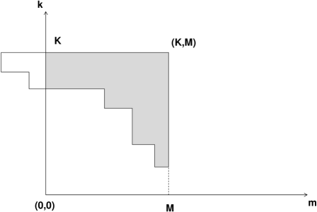
Figure 20: The domain (shadowed region), where the Hirota equation for $\tilde{Q}$’s is modified in the rectangle $0\leq k\leq K$, $0\leq m\leq M$. The diagram $\mu$ is reflected with respect to its vertical boundary.

Now we are ready to substitute (7.15) into the Hirota equation for $Q$’s (4.13). We have:

$$\begin{array}[]{lll}\phi_{\mu_{k,m}}(u)&=&\phi_{\mu_{k-1,m-1}}(u)\,\phi_{l^{\prime}_{k,m}}^{+}(u)\,\phi_{l_{k,m}}^{-}(u)\,\phi^{-1}(u)\\ &&\\ &=&\phi_{\mu_{k-1,m}}(u-2)\,\phi_{l^{\prime}_{k,m}}^{+}(u)\\ &&\\ &=&\phi_{\mu_{k,m-1}}(u+2)\,\phi_{l_{k,m}}^{-}(u)\,,\end{array}$$

provided $\mu_{k,m}$ is not empty (otherwise the right hand sides are equal to 1), where the “string polynomials” $\phi^{\pm}_{l}(u)$ are defined in (7.1) and (7.4). Using these obvious identities, it is straightforward to obtain the $\tilde{Q}\tilde{Q}$-relation:

$$\begin{array}[]{c}\phi\bigl{(}u+2l^{\prime}_{k,m}\bigr{)}\,\tilde{Q}_{k\!-\!1,m\!-\!1}(u)\,\tilde{Q}_{k,m}(u+2)\\ \\ -\,\,\,\,\phi\bigl{(}u\!-\!2l_{k,m}\!+\!2\bigr{)}\,\tilde{Q}_{k\!-\!1,m\!-\!1}(u+2)\,\tilde{Q}_{k,m}(u)\\ \\ =\,\,\,\tilde{Q}_{k-1,m}(u)\,\tilde{Q}_{k,m-1}(u+2)\,.\end{array}$$ (7.18)

In this form it is valid if $\mu_{k,m}\neq\emptyset$, otherwise the functions $\tilde{Q}$ obey the standard Hirota equation (4.13). In other words, the Hirota equation gets modified in the region shown in Fig.20. The boundary of this region in the $(k,m)$ plane is exactly the boundary of the diagram $\mu$. The functions $\tilde{Q}_{0,0}$ and $\tilde{Q}_{K,M}$ are fixed to be 1: $\tilde{Q}_{0,0}(u)=\tilde{Q}_{K,M}(u)=1$.

The Bethe equations are derived from (7.18) in the same way as in section 5. They acquire non-trivial right hand sides which can be compactly written in terms of the quantities $l_{k,m}$ and $l^{\prime}_{k,m}$:

$$\frac{\tilde{Q}_{k-1,m}\left(u_{j}^{(k,m)}\right)\tilde{Q}_{k,m}\left(u_{j}^{(k,m)}-2\right)\tilde{Q}_{k+1,m}\left(u_{j}^{(k,m)}+2\right)}{\tilde{Q}_{k-1,m}\left(u_{j}^{(k,m)}-2\right)\tilde{Q}_{k,m}\left(u_{j}^{(k,m)}+2\right)\tilde{Q}_{k+1,m}\left(u_{j}^{(k,m)}\right)}=\,-\,\frac{\phi\left(u_{j}^{(k,m)}+2l^{\prime}_{k,m}\right)}{\phi\left(u_{j}^{(k,m)}+2l^{\prime}_{k+1,m}\right)}\,,$$ (7.19)

$$\frac{\tilde{Q}_{k,m+1}\left(u_{j}^{(k,m)}\right)\tilde{Q}_{k,m}\left(u_{j}^{(k,m)}-2\right)\tilde{Q}_{k,m-1}\left(u_{j}^{(k,m)}+2\right)}{\tilde{Q}_{k,m+1}\left(u_{j}^{(k,m)}-2\right)\tilde{Q}_{k,m}\left(u_{j}^{(k,m)}+2\right)\tilde{Q}_{k,m-1}\left(u_{j}^{(k,m)}\right)}=\,-\,\frac{\phi\left(u_{j}^{(k,m)}-2l_{k,m+1}\right)}{\phi\left(u_{j}^{(k,m)}-2l_{k,m}\right)}\,,$$ (7.20)

$$\frac{\tilde{Q}_{k+1,m}\left(u_{j}^{(k,m)}\right)\tilde{Q}_{k,m-1}\left(u_{j}^{(k,m)}+2\right)}{\tilde{Q}_{k+1,m}\left(u_{j}^{(k,m)}+2\right)\tilde{Q}_{k,m-1}\left(u_{j}^{(k,m)}\right)}=\,\frac{\phi\left(u_{j}^{(k,m)}+2l_{k+1,m}^{\prime}\right)}{\phi\left(u_{j}^{(k,m)}-2l_{k,m}\right)}\,,$$ (7.21)

$$\frac{\tilde{Q}_{k,m+1}\left(u_{j}^{(k,m)}\right)\tilde{Q}_{k-1,m}\left(u_{j}^{(k,m)}-2\right)}{\tilde{Q}_{k,m+1}\left(u_{j}^{(k,m)}-2\right)\tilde{Q}_{k-1,m}\left(u_{j}^{(k,m)}\right)}=\,\frac{\phi\left(u_{j}^{(k,m)}-2l_{k,m+1}\right)}{\phi\left(u_{j}^{(k,m)}+2l_{k,m}^{\prime}\right)}\,,$$ (7.22)

These equations are listed here in the same order as equations (5.2)-(5.5). For empty diagrams, $l_{k,m}$ and $l^{\prime}_{k,m}$ are put equal to $0$. Using formulas (7.17), we can represent the right hand sides in a more explicit but less compact form:

$$\frac{\tilde{Q}_{k-1,m}\left(u_{j}^{(k,m)}\right)\tilde{Q}_{k,m}\left(u_{j}^{(k,m)}-2\right)\tilde{Q}_{k+1,m}\left(u_{j}^{(k,m)}+2\right)}{\tilde{Q}_{k-1,m}\left(u_{j}^{(k,m)}-2\right)\tilde{Q}_{k,m}\left(u_{j}^{(k,m)}+2\right)\tilde{Q}_{k+1,m}\left(u_{j}^{(k,m)}\right)}=\,-\,\frac{\phi\left(u_{j}^{(k,m)}\!+\!2m\!-\!2M\!+\!2\mu_{K-k+1}\right)}{\phi\left(u_{j}^{(k,m)}\!+\!2m\!-\!2M\!+\!2\mu_{K-k}\right)}\,,$$ (7.23)

$$\frac{\tilde{Q}_{k,m+1}\left(u_{j}^{(k,m)}\right)\tilde{Q}_{k,m}\left(u_{j}^{(k,m)}-2\right)\tilde{Q}_{k,m-1}\left(u_{j}^{(k,m)}+2\right)}{\tilde{Q}_{k,m+1}\left(u_{j}^{(k,m)}-2\right)\tilde{Q}_{k,m}\left(u_{j}^{(k,m)}+2\right)\tilde{Q}_{k,m-1}\left(u_{j}^{(k,m)}\right)}=\,-\,\frac{\phi\left(u_{j}^{(k,m)}\!-\!2k\!+\!2K\!-\!2\mu_{M-m}^{\prime}\right)}{\phi\left(u_{j}^{(k,m)}\!-\!2k\!+\!2K\!-\!2\mu_{M-m+1}^{\prime}\right)}\,,$$ (7.24)

$$\frac{\tilde{Q}_{k+1,m}\left(u_{j}^{(k,m)}\right)\tilde{Q}_{k,m-1}\left(u_{j}^{(k,m)}+2\right)}{\tilde{Q}_{k+1,m}\left(u_{j}^{(k,m)}+2\right)\tilde{Q}_{k,m-1}\left(u_{j}^{(k,m)}\right)}=\,\frac{\phi\left(u_{j}^{(k,m)}\!+\!2m\!-\!2M\!+\!2\mu_{K-k}\right)}{\phi\left(u_{j}^{(k,m)}\!-\!2k\!+\!2K\!-\!2\mu_{M-m+1}^{\prime}\right)}\,,$$ (7.25)

$$\frac{\tilde{Q}_{k,m+1}\left(u_{j}^{(k,m)}\right)\tilde{Q}_{k-1,m}\left(u_{j}^{(k,m)}-2\right)}{\tilde{Q}_{k,m+1}\left(u_{j}^{(k,m)}-2\right)\tilde{Q}_{k-1,m}\left(u_{j}^{(k,m)}\right)}=\,\frac{\phi\left(u_{j}^{(k,m)}\!-\!2k\!+\!2K\!-\!2\mu_{M-m}^{\prime}\right)}{\phi\left(u_{j}^{(k,m)}\!+\!2m\!-\!2M\!+\!2\mu_{K-k+1}\right)}\,.$$ (7.26)

These equations are the building blocks to make up the chain of Bethe equations for any undressing path.

For example, the chain of the Bethe equations for the simplest path $(K,M)\longrightarrow(0,M)\longrightarrow(0,0)$ is as follows. Moving down from $(K,M)$ to $(0,M)$, we have the equations

$$\frac{\tilde{Q}_{k-1,M}\left(u_{j}^{(k,M)}\right)\tilde{Q}_{k,M}\left(u_{j}^{(k,M)}-2\right)\tilde{Q}_{k+1,M}\left(u_{j}^{(k,M)}+2\right)}{\tilde{Q}_{k-1,M}\left(u_{j}^{(k,M)}-2\right)\tilde{Q}_{k,M}\left(u_{j}^{(k,M)}+2\right)\tilde{Q}_{k+1,M}\left(u_{j}^{(k,M)}\right)}=\,-\,\frac{\phi\left(u_{j}^{(k,M)}\!+\!2\mu_{K-k+1}\right)}{\phi\left(u_{j}^{(k,M)}\!+\!2\mu_{K-k}\right)}\,,$$ (7.27)

where $k=1,2,\ldots,K-1$. They agree with the chain of Bethe equations presented in [47, 48] for the bosonic case. At the corner, the equation is

$$\frac{\tilde{Q}_{1,M}\left(u_{j}^{(0,M)}\right)\tilde{Q}_{0,M-1}\left(u_{j}^{(0,M)}+2\right)}{\tilde{Q}_{1,M}\left(u_{j}^{(0,M)}+2\right)\tilde{Q}_{0,M-1}\left(u_{j}^{(0,M)}\right)}=\,\frac{\phi\left(u_{j}^{(0,M)}\!+\!2\mu_{K}\right)}{\phi\left(u_{j}^{(0,M)}\!+\!2K\!-\!2\mu_{1}^{\prime}\right)}\,,$$ (7.28)

Finally, moving to the left from $(0,M)$ to $(0,0)$, we have the equations

$$\frac{\tilde{Q}_{0,m+1}\left(u_{j}^{(0,m)}\right)\tilde{Q}_{0,m}\left(u_{j}^{(0,m)}-2\right)\tilde{Q}_{0,m-1}\left(u_{j}^{(0,m)}+2\right)}{\tilde{Q}_{0,m+1}\left(u_{j}^{(0,m)}-2\right)\tilde{Q}_{0,m}\left(u_{j}^{(0,m)}+2\right)\tilde{Q}_{0,m-1}\left(u_{j}^{(0,m)}\right)}=\,-\,\frac{\phi\left(u_{j}^{(0,m)}\!+\!2K\!-\!2\mu_{M-m}^{\prime}\right)}{\phi\left(u_{j}^{(0,m)}\!+\!2K\!-\!2\mu_{M-m+1}^{\prime}\right)}\,,$$ (7.29)

where $m=1,2,\ldots,M-1$. One can see that the differences of arguments of the $\phi$-functions in the numerator and the denominator are equal to the doubled Kac-Dynkin labels (A2) corresponding to the diagram $\mu$.

One can also write down the chain of equations for an arbitrary path, similarly to eq. (5.8). However, the general form of the right hand sides is not very illuminating.

The last remark concerns the form of the ansatz (7.15). Instead of (7.15) one could use a similar ansatz

$$Q_{k,m}(u)=\bar{\phi}_{\mu_{k,m}}\left(u\!+\!2(K\!-\!k)\!-\!2(M\!-\!m)\right)\,\bar{Q}_{k,m}(u)$$ (7.30)

with the function $\bar{\phi}_{\mu}(u)$ defined in (7.14). This leads to a similar system of Bethe equations with non-trivial vacuum parts. There is a one-to-one correspondence between solutions of the both systems.

8 Examples

8.1 Baxter and Bethe equations for $gl(1|1)$

Let us consider in detail the $gl(1|1)$ case. In this case all elements of transfer matrix $T_{1,1}(a,s,u)\equiv T(a,s,u)$ lay on the boundaries of the fat hook domain, as we see in Fig. 21. We read off from this figure:

$$T(0,0,u) = Q_{1,1}(u)\equiv\phi(u)=\prod_{j=1}^{N}\left(u-\theta_{j}\right)$$

$$T(a,0,u) = Q_{1,1}(u+a),\qquad a\geq 0$$

$$T(0,s,u) = Q_{1,1}(u-s),\qquad-\infty<s<\infty$$

$$T(a,1,u) = (-1)^{a-1}Q_{1,0}(u+a+1)Q_{0,1}(u-a-1),\qquad a\geq 1$$

$$T(1,s,u) = Q_{1,0}(u+s+1)Q_{0,1}(u-s-1),\qquad s\geq 1\,.$$ (8.1)

Using the Hirota equation (4.13) we get the only nontrivial $QQ$-relation:

$$Q_{0,0}(u)Q_{1,1}(u+2)-Q_{1,1}(u)Q_{0,0}(u+2) = Q_{0,1}(u)Q_{1,0}(u+2),$$

which gives, together with $Q_{0,0}(u)=1$,

$$Q_{1,0}(u)Q_{0,1}(u-2)=\phi(u)-\phi(u-2).$$ (8.2)

This relation allows us to exclude, for example, $Q_{0,1}$ or $Q_{1,0}$ from eq.(8.1) and to obtain, in particular, the Baxter $TQ$-relations:

$$T(1,s,u) = \frac{Q_{0,1}(u-s-1)}{Q_{0,1}(u+s-1)}\left(\phi(u+s+1)-\phi(u+s-1)\right)\,,$$

$$T(1,s,u) = \frac{Q_{1,0}(u+s+1)}{Q_{1,0}(u-s+1)}\left(\phi(u-s+1)-\phi(u-s-1)\right).$$ (8.3)

From the second relation, using regularity of the left hand side, we obtain the following Bethe equation:

$$1=\frac{\phi(u_{j}^{(1,0)})}{\phi(u_{j}^{(1,0)}-2)}.$$ (8.4)

It is a free fermion equation. We can also obtain it from the undressing procedure $Q_{1,1}\to Q_{1,0}\to Q_{0,0}=1$, putting $u=u^{(1,0)}+s-1$ in eq.(8.2). For another undressing procedure, $Q_{1,1}\to Q_{0,1}\to Q_{0,0}=1$, or by canceling poles at $u=u^{(0,1)}-s+1$ in the first equation in (8.1), we get the Bethe equation

$$1=\frac{\phi(u_{j}^{(0,1)})}{\phi(u_{j}^{(0,1)}+2)}.$$ (8.5)

Note that the Bethe equations (8.4), (8.5) do not depend on the representation parameter $s$ whereas the eigenvalues $T(1,s,u)$ do depend on it. In principle, nothing prevents this parameter to be continued analytically to the complex plane. This is precisely the continuous label of typical (long) irreducible representations [21] of the superalgebra in auxiliary space.

Let us consider higher rectangular irreps in the physical space. To cover representations with an arbitrary spin $\ell$ (one-row diagrams with $\ell$ boxes), we take a special form of the function $\phi(u)$, as in eq. (7.1):

$$\phi(u)=\varphi(u)\varphi(u+2)\dots\varphi(u+2\ell)\varphi\left(u+2(\ell-1)\right),$$ (8.6)

describing a “string” of length $\ell$. (Comparing to the previous section, we have changed the notation slightly denoting the polynomial function with roots $\theta_{i}$ by $\varphi(u)=\prod_{j}(u-\theta_{j})$.) According to (7.15), we have:

$$\begin{array}[]{lll}Q_{0,1}(u)&=&\tilde{Q}_{0,1}(u)\\ &&\\ Q_{1,0}(u)&=&\varphi(u)\varphi(u+2)\ldots\varphi(u+2(\ell-2))\,\tilde{Q}_{1,0}(u)\,.\end{array}$$

From the first equation in (8.1) we obtain the transfer matrix $T_{1,1}(1,s,u)\equiv T(1,s,u)$:

$$T(1,s,u+1)=\frac{\tilde{Q}_{0,1}(u-s)}{\tilde{Q}_{0,1}(u+s)}\left[\varphi(u+s+2\ell)-\varphi(u+s)\right]\,\,\,\prod_{j=1}^{\ell-1}\varphi(u+s+2j).$$ (8.7)

The last factor represents trivial zeros of $T(a,s,u)$. It has the same origin as the one in eq. (7.2). However, one should note that because $T(1,s,u)$ lives on the interior boundary, this factor contains more zeros than the one in eq. (7.2) (see the remark in the end of section 7.1). The Bethe equation (8.5) becomes:

$$1=\frac{\varphi(u_{j}^{(0,1)})}{\varphi(u_{j}^{(0,1)}+2\ell)}.$$ (8.8)

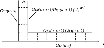
Figure 21: Boundary conditions for the transfer matrix $T(a,s,u)\equiv T_{1,1}(a,s,u)$ for the $gl(1|1)$ superalgebra.

It is easy to generalize these results to the case of an arbitrary physical spin $\ell_{l}$ at each site $l=1,2,\ldots,N$ of the chain. In this case we take

$$\phi(u)=\prod_{l=1}^{N}(u-\theta_{l})(u-\theta_{l}+2)\ldots(u-\theta_{l}+2\ell_{l}-2).$$

This yields the transfer matrix

$$T(1,s,u+1)=\frac{\tilde{Q}_{0,1}(u-s)}{\tilde{Q}_{0,1}(u+s)}\left(\prod_{l=1}^{N}\left(u-\theta_{l}+s+2\ell_{l}\right)-\prod_{l=1}^{N}\left(u-\theta_{l}+s\right)\right)\prod_{l=1}^{N}\prod_{j=0}^{\ell_{l}-2}(u-\theta_{l}+s+2j).$$ (8.9)

The last factor represents the trivial zeros which can be absorbed by normalization. Introducing a new renormalized function $T^{\prime}$ with the trivial zeroes removed,

$$T(1,s,u+1)=T^{\prime}(1,s,u+1)\,\,\prod_{l=1}^{N}\prod_{j=1}^{\ell_{l}-1}(u-\theta_{l}+s+2j)$$ (8.10)

we obtain, redefining the parameters $\theta_{l}=\hat{\theta}_{l}+\ell_{l}$,

$$T^{\prime}(1,s,u+1)=\frac{\tilde{Q}_{0,1}(u-s)}{\tilde{Q}_{0,1}(u+s)}\left(\prod_{l=1}^{N}\left(u-\hat{\theta}_{l}+s+\ell_{l}\right)-\prod_{l=1}^{N}\left(u-\hat{\theta}_{l}+s-\ell_{l}\right)\right)$$ (8.11)

which is essentially the same transfer matrix eigenvalue as for the rational limit of the equations (A.9), (A.10) from [53], with the definition of the $gl(1|1)$ $S$-matrix (3.1), (3.2) from [54]. The Bethe equations are

$$1=\prod_{l(\neq j)=1}^{N}\frac{u_{j}^{(0,1)}-\hat{\theta}_{l}+s+\ell_{l}}{u_{j}^{(0,1)}-\hat{\theta}_{l}+s-\ell_{l}}.$$ (8.12)

For the complete comparison one should exchange in these papers the parameters $\ell\rightarrow s,\,\,s\to r$ of the auxiliary and quantum spaces and take the rational limit. Some simple shifts in the arguments and definitions of Bethe roots are also necessary. Note that unlike [53], where they are the soliton charges, both representation labels $\ell$ and $s$ can be now considered as continuous parameters of the typical representation of $gl(1|1)$. This corresponds to the limit of large charges and large period of these soliton charges.

8.2 Baxter and Bethe equations for $gl(2|1)$

In the $gl(2|1)$ case, the transfer matrices $T_{2,1}(a,s,u)\equiv T(a,s,u)$ are on the boundaries of the fat hook except $T(1,s,u)$ in the middle row, as we see in Fig. 22. There are six $Q$-functions $Q_{k,m}(u)$ ($k=0,1,2;\,m=0,1$), two of them being fixed by the boundary conditions. The $T$-functions are expressed through them in the following way:

$$T(0,0,u) = Q_{2,1}(u)\equiv\phi(u)=\prod_{j=1}^{N}\left(u-\theta_{j}\right)$$

$$T(a,0,u) = Q_{2,1}(u+a),\qquad a\geq 0$$

$$T(0,s,u) = Q_{2,1}(u-s),\qquad-\infty<s<\infty$$

$$T(a,1,u) = Q_{2,0}(u+a+1)Q_{0,1}(u-a-1)(-1)^{a-2},\qquad a\geq 2$$

$$T(2,s,u) = Q_{2,0}(u+s+2)Q_{0,1}(u-s-2),\qquad s\geq 1\,.$$ (8.13)

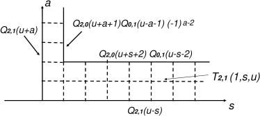
Figure 22: Boundary conditions for $T(a,s,u)\equiv T_{2,1}(a,s,u)$ for the $gl(2|1)$ superalgebra.

8.2.1 Baxter equations for the Kac-Dynkin diagram ${}_{1}\bigotimes\!\!-\!\!\!-\!\!\!-\!\!\bigodot$

(Here and below the subscript $1$ means the fundamental representation in the quantum space.)

The operator generating series (4.15) reads

$$\sum_{a=0}^{\infty}\frac{T(a,1,u+a+1)}{Q_{2,1}(u+2a+2)}\,e^{2a\partial_{u}}=\hat{U}_{1,0}\hat{U}_{2,0}\hat{V}^{-1}_{2,0}=$$ (8.14)

$$= \left(\frac{Q_{1,0}(u)}{Q_{1,0}(u+2)}-e^{2\partial_{u}}\right)\left(\frac{Q_{2,0}(u)}{Q_{2,0}(u+2)}\frac{Q_{1,0}(u+2)}{Q_{1,0}(u)}-e^{2\partial_{u}}\right)\left(\frac{Q_{2,0}(u)}{Q_{2,0}(u+2)}\frac{Q_{2,1}(u+2)}{Q_{2,1}(u)}-e^{2\partial_{u}}\right)^{-1}.$$

In particular,

$$\frac{T(2,1,u+3)}{\phi(u+4)}= \frac{Q_{2,0}(u+6)}{Q_{2,0}(u+4)}\frac{\phi(u+4)}{\phi(u+6)}-\frac{Q_{1,0}(u+4)}{Q_{1,0}(u+2)}\frac{Q_{2,0}(u+6)}{Q_{2,0}(u+4)}\frac{\phi(u+2)}{\phi(u+6)}$$ (8.15)

$$- \frac{Q_{1,0}(u)}{Q_{1,0}(u+2)}\frac{Q_{2,0}(u+6)}{Q_{2,0}(u+2)}\frac{\phi(u+2)}{\phi(u+6)}+\frac{Q_{2,0}(u+6)}{Q_{2,0}(u+2)}\frac{\phi(u)}{\phi(u+6)}\,.$$

From this equation and equation

$$T(2,s,u)=\frac{Q_{2,0}(u+s+2)}{Q_{2,0}(u-s+4)}\,T(2,1,u-s+1)$$

which follows from eq.(8.2), we obtain

$$\frac{T(2,s,u)}{\phi(u-s+2)} = \frac{Q_{2,0}(u+s+2)}{Q_{2,0}(u-s+2)}\frac{\phi(u-s+2)}{\phi(u-s+4)}-\frac{Q_{1,0}(u-s+2)}{Q_{1,0}(u-s)}\frac{Q_{2,0}(u+s+2)}{Q_{2,0}(u-s+2)}\frac{\phi(u-s)}{\phi(u-s+4)}$$ (8.16)

$$- \frac{Q_{1,0}(u-s-2)}{Q_{1,0}(u-s)}\frac{Q_{2,0}(u+s+2)}{Q_{2,0}(u-s)}\frac{\phi(u-s)}{\phi(u-s+4)}+\frac{Q_{2,0}(u+s+2)}{Q_{2,0}(u-s)}\frac{\phi(u-s-2)}{\phi(u-s+4)}\,.$$

Note that the representation index $s$ can be treated as a continuous parameter. It corresponds to the continuous label of typical representations of the $gl(2|1)$ superalgebra.

8.2.2 Spins in higher irreps in the quantum space

As an illustrative example to section 5, as well as for the purpose of comparison with the result of [6] (eq.(E1) obtained from the specific $S$-matrix by the algebraic Bethe Ansatz), we consider here spins in the quantum space in the irrep $(r^{2})$ (Young diagrams with two rows of length $r$). At the end, the number $r$ will be treated as a continuous label.

Let us introduce new definitions, following eq. (7.7) of the previous section:

$$\phi(u)\equiv\phi_{2,1}(u)=\varphi(u-2)\left[\varphi^{2}(u)\varphi^{2}(u+2)\dots\varphi^{2}\left(u+2r-4\right)\right]\varphi\left(u+2r-2\right),$$ (8.17)

$$\phi_{2,0}(u)=\varphi(u-2)\left[\varphi^{2}(u)\varphi^{2}(u+2)\dots\varphi^{2}\left(u+2r-6\right)\right]\varphi\left(u+2r-4\right)\,,$$ (8.18)

$$\phi_{1,0}(u)=\varphi(u)\varphi(u+2)\dots\varphi\left(u+2r-4\right).$$ (8.19)

Here $\varphi(u)=\prod_{j}(u-\theta_{j})$. Then, according to eq. (7.15),

$$Q_{2,0}(u)=\phi_{2,0}(u)\,\tilde{Q}_{2,0}(u)\,,$$ (8.20)

$$Q_{1,0}(u)=\phi_{1,0}(u)\,\tilde{Q}_{1,0}(u)\,.$$ (8.21)

In this notation, eq.(8.16) takes the form

$$T^{\prime}(2,s,u) = \frac{\tilde{Q}_{2,0}(u+s+2)}{\tilde{Q}_{2,0}(u-s+2)}$$

$$- \frac{\tilde{Q}_{1,0}(u-s+2)}{\tilde{Q}_{1,0}(u-s)}\frac{\tilde{Q}_{2,0}(u+s+2)}{\tilde{Q}_{2,0}(u-s+2)}\frac{\phi_{1,0}(u-s+2)}{\phi_{1,0}(u-s)}\frac{\phi(u-s)}{\phi(u-s+2)}$$

$$- \frac{\tilde{Q}_{1,0}(u-s-2)}{\tilde{Q}_{1,0}(u-s)}\frac{\tilde{Q}_{2,0}(u+s+2)}{\tilde{Q}_{2,0}(u-s)}\frac{\phi_{1,0}(u-s-2)}{\phi_{1,0}(u-s)}\frac{\phi_{2,0}(u-s+2)}{\phi_{2,0}(u-s)}\frac{\phi(u-s)}{\phi(u-s+2)}$$

$$+ \frac{\tilde{Q}_{2,0}(u+s+2)}{\tilde{Q}_{2,0}(u-s)}\frac{\phi_{2,0}(u-s+2)}{\phi_{2,0}(u-s)}\frac{\phi(u-s-2)}{\phi(u-s+2)}\,,$$

where we redefined the transfer matrix extracting trivial zeros:

$$T(2,s,u) = T^{\prime}(2,s,u)\,\frac{\phi^{2}(u-s+2)}{\phi(u-s+4)}\frac{\phi_{2,0}(u+s+2)}{\phi_{2,0}(u-s+2)}=$$ (8.22)

$$= T^{\prime}(2,s,u)\,\,\left[\varphi(u-s)\varphi(u-s+2)\phi_{2,0}(u+s+2)\right].$$

For the reason already discussed in the case of $gl(1|1)$, $T^{\prime}$ is not equal to $\tilde{T}$ of eq.(7.10).

Calculating the ratios of $\phi$-functions in eq.(8.2.2), we find for the following result for the transfer matrix in physical irrep $(r^{2})$ and the auxiliary irrep $(s^{2})$:

$$T^{\prime}_{r}(2,s,u) = \frac{\tilde{Q}_{2,0}(u+s+2)}{\tilde{Q}_{2,0}(u-s+2)}$$ (8.23)

$$- \frac{\tilde{Q}_{1,0}(u-s+2)}{\tilde{Q}_{1,0}(u-s)}\frac{\tilde{Q}_{2,0}(u+s+2)}{\tilde{Q}_{2,0}(u-s+2)}\frac{\varphi(u-s-2)}{\varphi(u-s+2r)}$$

$$- \frac{\tilde{Q}_{1,0}(u-s-2)}{\tilde{Q}_{1,0}(u-s)}\frac{\tilde{Q}_{2,0}(u+s+2)}{\tilde{Q}_{2,0}(u-s)}\frac{\varphi(u-s-2)}{\varphi(u-s+2r)}$$

$$+ \frac{\tilde{Q}_{2,0}(u+s+2)}{\tilde{Q}_{2,0}(u-s)}\frac{\varphi(u-s-4)}{\varphi(u-s+2r-2)}\frac{\varphi(u-s-2)}{\varphi(u-s+2r)}\,.$$

Using the notation of eq.(5.9) $\tilde{Q}_{k+m}(u)=\tilde{Q}_{k,m}(u+k-m)$ and setting $\tilde{\varphi}(u)=\varphi(u+r-1)$ we bring eq.(8.23) to the form

$$T^{\prime}_{r}(2,s,u) = \frac{\tilde{Q}_{2}(u+s)}{\tilde{Q}_{2}(u-s)}$$ (8.24)

$$- \frac{\tilde{Q}_{1}(u-s+1)}{\tilde{Q}_{1}(u-s-1)}\frac{\tilde{Q}_{2}(u+s)}{\tilde{Q}_{2}(u-s)}\frac{\tilde{\varphi}(u-s-r-1)}{\tilde{\varphi}(u-s+r+1)}$$

$$- \frac{\tilde{Q}_{1}(u-s-3)}{\tilde{Q}_{1}(u-s-1)}\frac{\tilde{Q}_{2}(u+s)}{\tilde{Q}_{2}(u-s-2)}\frac{\tilde{\varphi}(u-s-r-1)}{\tilde{\varphi}(u-s+r+1)}$$

$$+ \frac{\tilde{Q}_{2}(u+s)}{\tilde{Q}_{2}(u-s-2)}\frac{\tilde{\varphi}(u-s-r-3)}{\tilde{\varphi}(u-s+r-1)}\frac{\tilde{\varphi}(u-s-r-1)}{\tilde{\varphi}(u-s+r+1)}\,.$$

This transfer matrix eigenvalue coincides, after shifting $r\to r-1$ and making an easy generalization to the inhomogeneous chain (i.e., to spins in arbitrary irreps at each site of the chain), with eq.(E1) taken from [6] (see Appendix E, where their result is rewritten in our notation). Note also that the spin label $r$, as well as $s$, can be treated as continuous parameters here. Hence our method is general enough to describe the transfer matrices in all possible typical and atypical irreps in quantum and auxiliary spaces.

Canceling the poles at $u=u^{(2,0)}_{j}+s-2$ and $u=u^{(1,0)}_{j}+s$ in eq.(8.23), we write the following Bethe equations:

$$\frac{\varphi\left(u^{(2,0)}_{j}+2r-2\right)}{\varphi\left(u^{(2,0)}_{j}-4\right)} = \frac{\tilde{Q}_{1,0}\left(u^{(2,0)}_{j}\right)}{\tilde{Q}_{1,0}\left(u^{(2,0)}_{j}-2\right)}$$

$$-1 = \frac{\tilde{Q}_{1,0}\left(u^{(1,0)}_{j}+2\right)}{\tilde{Q}_{1,0}\left(u^{(1,0)}_{j}-2\right)}\frac{\tilde{Q}_{2,0}\left(u^{(1,0)}_{j}\right)}{\tilde{Q}_{2,0}\left(u^{(1,0)}_{j}+2\right)},$$ (8.25)

or, in the notation of eq. (8.24),

$$\frac{\tilde{\varphi}\left(u^{(2)}_{j}+r+1\right)}{\tilde{\varphi}\left(u^{(2)}_{j}-r-1\right)} = \frac{\tilde{Q}_{1}\left(u^{(2)}_{j}+1\right)}{\tilde{Q}_{1}\left(u^{(2)}_{j}-1\right)}$$

$$-1 = \frac{\tilde{Q}_{1}\left(u^{(1)}_{j}+2\right)}{\tilde{Q}_{1}\left(u^{(1)}_{j}-2\right)}\frac{\tilde{Q}_{2}\left(u^{(1)}_{j}-1\right)}{\tilde{Q}_{2}\left(u^{(1)}_{j}+1\right)}.$$ (8.26)

As an example, let us also consider two other equations for different choices of the Kac-Dynkin diagram.

8.2.3 Bethe equations for the Kac-Dynkin diagram $\bigotimes\!\!-\!\!\!-\!\!\!-\!\!\bigodot_{1}$

Let us express $T(1,s,u)$ through $Q$’s using eq.(4.1):

$$\sum_{a=0}^{\infty}\frac{T(a,1,u+a+1)}{Q_{2,1}(u+2a+2)}\,e^{2a\partial_{u}}=\hat{V}^{-1}_{0,0}\hat{U}_{1,1}\hat{U}_{2,1}=$$

$$= \left(\frac{Q_{0,1}(u+2)}{Q_{0,1}(u)}-e^{2\partial_{u}}\right)^{-1}\left(\frac{Q_{1,1}(u)}{Q_{1,1}(u+2)}\frac{Q_{0,1}(u+2)}{Q_{0,1}(u)}-e^{2\partial_{u}}\right)\left(\frac{Q_{2,1}(u)}{Q_{2,1}(u+2)}\frac{Q_{1,1}(u+2)}{Q_{1,1}(u)}-e^{2\partial_{u}}\right).$$

In particular,

$$\frac{T(1,1,u+2)}{\phi(u+4)}=-\frac{Q_{1,1}(u)}{Q_{1,1}(u+2)}-\frac{Q_{0,1}(u)}{Q_{0,1}(u+2)}\frac{\phi(u+2)}{\phi(u+4)}\frac{Q_{1,1}(u+4)}{Q_{1,1}(u+2)}+\frac{Q_{0,1}(u)}{Q_{0,1}(u+2)}\frac{\phi(u+2)}{\phi(u+4)}.$$ (8.28)

Canceling the poles in eq.(8.28), it is straightforward to write the following Bethe equations for $gl(2|1)$ superalgebra:

$$\frac{\phi\left(u^{(1,1)}_{j}+4\right)}{\phi\left(u^{(1,1)}_{j}+2\right)} = \frac{Q_{0,1}\left(u^{(1,1)}_{j}\right)}{Q_{0,1}\left(u^{(1,1)}_{j}+2\right)}\frac{Q_{1,1}\left(u^{(1,1)}_{j}+4\right)}{Q_{1,1}\left(u^{(1,1)}_{j}\right)}$$

$$1 = \frac{Q_{1,1}\left(u^{(0,1)}_{j}+4\right)}{Q_{1,1}\left(u^{(0,1)}_{j}+2\right)}.$$ (8.29)

8.2.4 Bethe equations for the Kac-Dynkin diagram $\bigotimes\!\!-\!\!\!-\!\!\!-\!\!\bigotimes_{1}$

Using eq.(4.16) or eq.(4.15), we write the operator generating series:

$$\sum_{a=0}^{\infty}\frac{T(a,1,u+a+1)}{Q_{2,1}(u+2a+2)}\,e^{2a\partial_{u}}=\hat{U}_{1,0}\hat{V}^{-1}_{1,0}\hat{U}_{2,1}=$$

$$= \left(\frac{Q_{1,0}(u)}{Q_{1,0}(u+2)}-e^{2\partial_{u}}\right)\left(\frac{Q_{1,0}(u)}{Q_{1,0}(u+2)}\frac{Q_{1,1}(u+2)}{Q_{1,1}(u)}-e^{2\partial_{u}}\right)^{-1}\left(\frac{Q_{2,1}(u)}{Q_{2,1}(u+2)}\frac{Q_{1,1}(u+2)}{Q_{1,1}(u)}-e^{2\partial_{u}}\right).$$

In particular,

$$\frac{T(1,1,u+2)}{\phi(u+3)}=-\frac{Q_{1,0}(u+4)}{Q_{1,0}(u+2)}\frac{\phi(u+2)}{\phi(u+4)}+\frac{Q_{1,0}(u+4)}{Q_{1,0}(u+2)}\frac{Q_{1,1}(u)}{Q_{1,1}(u+2)}\frac{\phi(u+2)}{\phi(u+4)}-\frac{Q_{1,1}(u)}{Q_{1,1}(u+2)}.$$ (8.31)

Canceling the poles in eq.(8.31), we write the following Bethe equations:

$$1 = \frac{Q_{1,1}\left(u^{(1,0)}_{j}\right)}{Q_{1,1}\left(u^{(1,0)}_{j}-2\right)}$$

$$\frac{\phi\left(u^{(1,1)}_{j}\right)}{\phi\left(u^{(1,1)}_{j}+2\right)} = \frac{Q_{1,0}\left(u^{(1,1)}_{j}\right)}{Q_{1,0}\left(u^{(1,1)}_{j}+2\right)}.$$ (8.32)

8.3 Examples of the integration algorithm

To illustrate the general algorithm of section 6, we apply it to $gl(2)$, $gl(2|1)$ and $gl(2|2)$ (super)algebras.

8.3.1 $gl(2)$ algebra

In this case equation (6.36) reads

$$T_{2,0}(1,s,u)=\widehat{H}^{-1}_{2^{-},0}(0,s,u)~{}T_{1,0}(1,s,u),\quad 0\leq s<\infty.$$ (8.33)

Substituting explicit expressions for $\widehat{H}^{-1}_{2^{-},0}(0,s,u)$ (6.1) and $T_{1,0}(1,s,u)$ (6.34), we immediately obtain the explicit formula for non-vanishing functions which do not belong to the boundaries:

$$T_{2,0}(1,s,u+s-1)=Q_{1,0}(u+2s)Q_{1,0}(u-2)\sum_{j=0}^{s}\frac{Q_{2,0}(u+2j)}{Q_{1,0}(u+2j-2)Q_{1,0}(u+2j)}.$$ (8.34)

8.3.2 $gl(2|1)$ superalgebra

In this case equation (6.36) reads

$$T_{2,1}(1,s,u)=\widehat{H}_{2,0^{+}}(0,s,u)~{}\widehat{H}^{-1}_{2^{-},0}(0,s,u)~{}T_{1,0}(1,s,u)\equiv\widehat{H}_{2,0^{+}}(0,s,u)~{}T_{2,0}(1,s,u),\quad 0\leq s<\infty.$$ (8.35)

Substituting explicit expressions for $\widehat{H}_{2,0^{+}}(0,s,u)$ (6.1) and $T_{2,0}(1,s,u)$ (8.34), we obtain, after straightforward calculations, the following result for non-vanishing functions which do not belong to the boundaries:

$$T_{2,1}(1,s,u\!+\!s\!-\!1)=Q_{1,0}(u\!+\!2s)\left(\frac{Q_{2,1}(u)}{Q_{1,0}(u)}+Q_{1,1}(u\!-\!2)\sum_{j=0}^{s-1}\frac{Q_{2,0}(u+2j+2)}{Q_{1,0}(u+2j)Q_{1,0}(u+2j+2)}\,\theta(s\!-\!1)\right).$$ (8.36)

The step function $\theta(s)=1$ at $s\geq 0$ and $0$ otherwise. In the calculation, we have used eq. (3.45) to substitute

$$\frac{Q_{1,0}(u-2)Q_{2,1}(u)-Q_{1,0}(u)Q_{2,1}(u-2)}{Q_{2,0}(u)}=Q_{1,1}(u-2)\,.$$

8.3.3 $gl(2|2)$ superalgebra

In this case equations (6.36) and (6.37) read

$$T_{2,2}(1,s,u) = \widehat{H}_{2,1^{+}}(0,s,u)~{}\widehat{H}_{2,0^{+}}(0,s,u)~{}\widehat{H}^{-1}_{2^{-},0}(0,s,u)~{}T_{1,0}(1,s,u)$$ (8.37)

$$\equiv \widehat{H}_{2,1^{+}}(0,s,u)~{}\widehat{H}_{2,0^{+}}(0,s,u)~{}T_{2,0}(1,s,u)\equiv\widehat{H}_{2,1^{+}}(0,s,u)~{}T_{2,1}(1,s,u),\quad 0\leq s<\infty~{}~{}~{}~{}$$

and

$$T_{2,2}(a,1,u)=\widehat{H}_{1^{+},2}(a,0,u)~{}\widehat{H}_{0^{+},2}(a,0,u)~{}\widehat{H}^{-1}_{0,2^{-}}(a,0,u)~{}T_{0,1}(a,1,u),\quad 0\leq a<\infty\,.$$ (8.38)

Substituting explicit expressions for the shift operators, we finally obtain:

$$T_{2,2}(1,s,u+s-1)=Q_{1,0}(u+2s)\Big{(}\frac{Q_{2,2}(u)}{Q_{1,0}(u)}+\frac{Q_{2,2}(u)Q_{1,1}(u-2)Q_{2,0}(u+2)}{Q_{2,1}(u)Q_{1,0}(u)Q_{1,0}(u+2)}\,\theta(s-1)$$ (8.39)

$$- \frac{Q_{2,2}(u-2)Q_{2,1}(u+2)}{Q_{2,1}(u)Q_{1,0}(u+2)}\,\theta(s-1)+Q_{1,2}(u-2)\sum_{j=0}^{s-2}\frac{Q_{2,0}(u+2j+4)}{Q_{1,0}(u+2j+2)Q_{1,0}(u+2j+4)}\,\theta(s-2)\Big{)}~{}~{}~{}$$

and

$$T_{2,2}(a,1,u-a+1)=Q_{0,1}(u-2a)\Big{(}\frac{Q_{2,2}(u)}{Q_{0,1}(u)}+\frac{Q_{2,2}(u)Q_{1,1}(u+2)Q_{0,2}(u-2)}{Q_{1,2}(u)Q_{0,1}(u)Q_{0,1}(u-2)}\,\theta(a-1)$$ (8.40)

$$+ \frac{Q_{2,2}(u+2)Q_{1,2}(u-2)}{Q_{1,2}(u)Q_{0,1}(u-2)}\theta(a-1)+Q_{2,1}(u+2)\sum_{j=0}^{a-2}\frac{(-1)^{j}Q_{0,2}(u-2j-4)}{Q_{0,1}(u-2j-2)Q_{0,1}(u-2j-4)}\,\theta(a-2)\Big{)}.~{}~{}~{}~{}$$

In the calculation, we have used eq. (3.45) to substitute

$$Q_{1,1}(u-2)Q_{2,2}(u)-Q_{1,1}(u)Q_{2,2}(u-2)=Q_{1,2}(u-2)Q_{2,1}(u)$$

and

$$\frac{Q_{0,1}(u)Q_{1,2}(u+2)-Q_{0,1}(u+2)Q_{1,2}(u)}{Q_{0,2}(u)}=Q_{1,1}(u+2).$$

The functions $T_{2,2}(1,s,u)$ and $T_{2,2}(a,1,u)$ form a complete set of non-vanishing $T$-functions which do not lie on the boundaries of the fat hook domain for the case of the $gl(2|2)$ superalgebra.

9 Discussion

In this paper we have dealt with finite dimensional representations of $gl(K|M)$ and the periodic spin chains based on the rational $R$-matrices. We believe that the method is powerful enough to incorporate various generalizations, such as extension to twisted and open spin chains, to infinite-dimensional representations of non-compact version of the symmetry group as well as to models with more general $R$-matrices, including various exotic ones, as the Hubbard $R$-matrix or the recently constructed AdS/CFT S-matrix. We expect that the Hirota relation should be the same for all these problems, with only difference being in the boundary and analyticity conditions.

For example, the extension to spin chains with twisted boundary conditions can be accomplished by replacing the polynomial $Q$-functions by “Bloch polynomials”, i.e., functions of the form $Q(u)=Ae^{\kappa u}\prod_{j}(u-u_{j})$, where $\kappa$ is related to the twisted boundary condition. This leads to appropriate simple modifications in the Bethe equations.

The extension to supersymmetric spin chains with trigonometric $R$-matrices is also straightforward. The Hirota equation and the boundary conditions remain the same. The only change is again in the analytical properties of the $T$-functions: in the trigonometric case they are “trigonometric polynomials”, i.e., finite products of $\sin(\eta(u-u_{j}))$ or $\mbox{sinh}\,(\eta(u-u_{j}))$. A hypothetical generalization to the elliptic case is much more interesting. As far as we know, supersymmetric quantum spin chains with elliptic $R$-matrices were never discussed in the literature. On the other hand, the bosonic case suggests [16] that the functional relations between commuting integrals of motion are given by the same Hirota equation. The solutions are sought in the form of “elliptic polynomials”, i.e., finite products of Jacobi theta-functions $\theta(\eta(u-u_{j})|\tau)$. From this point of view, it would be interesting to analyze elliptic polynomial solutions to the Hirota equation with boundary conditions of the fat hook type. They might solve (as yet hypothetical) supersymmetric quantum integrable models with elliptic $R$-matrices.

It is also important to elaborate, within the framework of Hirota equations, a more direct approach to spin chains in typical representations of superalgebras (the ones having a continuous label). One would like to understand them not only in the sense of analytic continuation with respect to the representation label (as we demonstrated in this paper by simple examples) but also to find their place on other levels of the construction. A characterization of solutions to the Hirota equation that are responsible for spin chains in typical representations would be of particular importance.

Appendix A. Superalgebras and their representations

For completeness, we list here some basic objects and notation related to Lie superalgebras $gl(K|M)$ and their representations. The main references are [19]-[22].

We use the notation $p(\alpha)$ for the ${\mathbb{Z}}_{2}$-grading of the index $\alpha$: $p(\alpha)=0$ if $\alpha$ is bosonic and $p(\alpha)=1$ if $\alpha$ is fermionic. The same notation is used to denote the grading of any objects (vectors, operators,…) with definite parity. Objects with definite parity are called homogeneous.

A matrix $A$ with matrix elements $A^{i}_{j}$ (we imply that they are usual numbers, i.e., $p(A^{i}_{j})=0$) is said to be even (odd) if $p(i)+p(j)$ is even (odd) for all non-vanishing elements of $A$. The $R$-matrix (2.1) is an even matrix.

Let $X$, $Y$ be two graded spaces, and let $e_{i}$, $f_{j}$ be the corresponding (homogeneous) basis vectors. For any two vectors $x=\sum_{i}x_{i}e_{i}$, $y=\sum_{i}y_{i}f_{i}$ we have

$$x\otimes y=\sum_{i,j}(x_{i}e_{i})\otimes(y_{j}f_{j})=\sum_{i,j}(-1)^{p(i)p(j)}x_{i}y_{j}\,(e_{i}\otimes f_{j})\,,$$

so the components of the vector $x\otimes y$ in the basis $e_{i}\otimes f_{j}$ are $(-1)^{p(i)p(j)}x_{i}y_{j}$. The action of the operator $A\otimes B$ in $X\otimes Y$ is defined on homogeneous objects as $A\otimes B\,(x\otimes y)=(-1)^{p(x)p(y)}A(x)\otimes B(y)$. Matrix elements of the tensor product of even matrices $A^{i}_{j}$, $B^{\alpha}_{\beta}$ are:

$$(A\otimes B)^{i\alpha}_{j\beta}=(-1)^{p(\alpha)(p(i)+p(j))}A^{i}_{j}B^{\alpha}_{\beta}\,.$$

This rule explains the origin of the sign factors in the graded Yang-Baxter equation.

The Lie superalgebra $gl(K|M)$ can be most transparently defined through its matrix realization: it is the set of block matrices

$$g=\left(\begin{array}[]{cc}A&B\\ C&D\end{array}\right)$$ (A1)

such that $A,B,C,D$ are respectively $K\times K$, $K\times M$, $M\times K$ and $M\times M$ matrices. The even subalgebra $gl(K|M)_{0}$ has $B=C=0$, the odd subalgebra $gl(K|M)_{1}$ has $A=D=0$. For homogeneous elements, the bracket is given by

$$[g,g^{\prime}]=gg^{\prime}-(-1)^{p(g)p(g^{\prime})}g^{\prime}g\,.$$

Note that $gl(K|M)_{0}=gl(K)\oplus gl(M)$. For elements $g$ realized as above the supertrace is defined by $\mbox{str}\,g=\mbox{tr}\,A-\mbox{tr}\,D$.

A basis for $gl(K|M)$ consists of matrices $E_{ij}$ with entry $1$ at position $(i,j)$ and $0$ otherwise. A Cartan subalgebra of $gl(K|M)$ is spanned by the elements $E_{ii}$, $i=1,\ldots,K+M$. The set of generators of $gl(K|M)$ consists of the $E_{ii}$ and the elements $E_{i,i+1}$ and $E_{i+1,i}$, $i=1,\ldots,K+M-1$. The space dual to the Cartan subalgebra is spanned by the linear forms $\epsilon_{i}:g\mapsto A_{ii}$ ($i=1,\ldots,K$) and $\delta_{i}:g\mapsto D_{ii}$ ($i=1,\ldots,M$), where $g$ is given by (A1). Let us choose the basis in the space dual to the Cartan subalgebra to be $\epsilon_{1},\ldots,\epsilon_{K},\delta_{1},\ldots,\delta_{M}$. On this space there is a bilinear form induced by the supertrace in the superalgebra:

$$(\epsilon_{i}|\epsilon_{j})=\delta_{ij}\,,\quad(\epsilon_{i}|\delta_{j})=(\delta_{i}|\epsilon_{j})=0\,,\quad(\delta_{i}|\delta_{j})=-\delta_{ij}\,.$$

Even (bosonic) roots are $\epsilon_{i}-\epsilon_{j}$ and $\delta_{i}-\delta_{j}$ ($i\neq j$), odd (fermionic) roots are $\pm(\epsilon_{i}-\delta_{j})$. There are several choices of simple root systems. The distinguished simple root system has the form $\alpha_{i}=\epsilon_{i}-\epsilon_{i+1}$ for $i=1,\ldots,K-1$, $\alpha_{K}=\epsilon_{K}-\delta_{1}$, $\alpha_{K+j}=\delta_{j}-\delta_{j+1}$ for $j=1,\ldots,M-1$. All other simple root systems are obtained from this one by reflections with respect to odd roots $\alpha$ with $(\alpha|\alpha)=0$.

Elements of the space dual to the Cartan subalgebra are called the weights. The weight is an expression of the form

$$\Lambda=\sum_{i=1}^{K}\Lambda_{i}\epsilon_{i}+\sum_{j=1}^{M}\bar{\Lambda}_{j}\delta_{j}\,.$$

Let $\lambda$ be a Young diagram formed by a sequence of non-negative non-increasing integers: $\lambda=(\lambda_{1},\lambda_{2},\ldots)$, $\lambda_{1}\geq\lambda_{2}\geq\ldots\geq 0$. To such a diagram one assigns the weight $\Lambda_{i}=\lambda_{i}$ ($i=1,\ldots,K)$, $\bar{\Lambda}_{j}=\bar{\lambda}_{j}$ $(j=1,\ldots,M)$, where $\bar{\lambda}_{j}=\mbox{max}\,(\lambda_{j}^{\prime}-K,\,0)$ and $\lambda^{\prime}_{j}$ is the height of the $j$-th column of the diagram $\lambda$. It is implied that $\lambda_{K+1}\leq M$.

A Kac-Dynkin label is a sequence $b_{1},b_{2},\ldots,b_{K},\ldots,b_{K+M-1}$, where all $b_{j}$ except $b_{K}$ are non-negative integers while $b_{K}$ may be any real number. There is a one-to-one correspondence between finite-dimensional irreducible representations (irreps) of the superalgebra $gl(K|M)$ and the Kac-Dynkin labels [19]. We consider covariant tensor irreps of the superalgebra $gl(K|M)$. One can assign the following Kac-Dynkin label to any highest weight $\Lambda$ associated with a Young diagram $\lambda$ as above:

$$\begin{array}[]{ll}b_{i}=\lambda_{i}-\lambda_{i+1}\,,&i=1,\ldots,K-1\,,\\ &\\ b_{K}=\lambda_{K}+\bar{\lambda}_{1}\,,&\\ &\\ b_{j+K}=\bar{\lambda}_{j}-\bar{\lambda}_{j+1}\,,&j=1,\ldots,M-1\,.\end{array}$$ (A2)

Therefore, one associates a tensor irrep of $gl(K|M)$ to any Young diagram. (The diagrams containing a rectangular subdiagram with $K+1$ rows and $M+1$ columns correspond to vanishing representations, so such diagrams are illegal, similarly to diagrams containing $K+1$ rows for $gl(K)$.) However, for superalgebras this correspondence is not one-to-one. Different Young diagrams may correspond to equivalent irreps (i.e., to the same Kac-Dynkin label). In particular, this is the case for rectangular diagrams when $M+n$ columns of $K$ boxes are replaced by $M$ columns of $K+n$ boxes [21].

There is a large class of finite-dimensional irreps of $gl(K|M)$ which cannot be associated with a Young diagram. Given an irreducible tensor representation with the highest weight $\Lambda$, there is a one-parametric family of finite-dimensional irreps with the highest weight $\Lambda(c)=\Lambda+c\sum_{i=1}^{K}\epsilon_{i}$, where $c$ is a real parameter. This yields the Kac-Dynkin label with a non-integer $b_{K}=\lambda_{K}+\bar{\lambda}_{1}+c$.

One distinguishes typical and atypical irreps [19] (in physical terminology, long and short irreps, respectively). An irrep with the highest weight $\Lambda$ is atypical iff there exists at least one pair $(i,j)$, $i=1,\ldots,K$, $j=1,\ldots,M$, such that

$$(\Lambda+\rho,\epsilon_{i}-\delta_{j})=0\,,$$ (A3)

where

$$\rho=\frac{1}{2}\sum_{i=1}^{K}(K-M-2i+1)\epsilon_{i}+\frac{1}{2}\sum_{j=1}^{M}(K+M-2j+1)\delta_{j}\,.$$

For typical irreps, there is no such pair $(i,j)$ that (A3) holds. All irreps with $b_{K}\geq M$ are typical. All rectangular irreps corresponding to diagrams having $a$ rows and $s$ columns with $a<K$ or $s<M$ are atypical.

Appendix B. Auxiliary linear problems for the Hirota equation

Let $\tau=\tau(p_{1},p_{2},p_{3})$ be a function of three variables. For brevity, we denote

$$\tau(p_{1}+1,p_{2},p_{3}):=\tau_{1},\quad\tau(p_{1},p_{2}+1,p_{3}):=\tau_{2},\quad\tau(p_{1}+1,p_{2}+1,p_{3}):=\tau_{12},\quad\mbox{etc.}$$

Let $\alpha\beta\gamma$ be any cyclic permutation of $123$. Consider the following system of three linear equations for a function $\psi=\psi(p_{1},p_{2},p_{3})$:

$$\left(e^{\partial_{\alpha}}+\lambda_{\gamma}\,\frac{\tau\,\tau_{\alpha\beta}}{\tau_{\alpha}\tau_{\beta}}\right)\psi=e^{\partial_{\beta}}\psi\,,\quad\alpha\beta\gamma=123,\;231,\;312,$$ (B1)

where $\lambda_{\alpha}$ are parameters and $\partial_{\alpha}\equiv\partial/\partial_{p_{\alpha}}$. Their compatibility implies the Hirota equation for $\tau$:

$$\lambda_{1}\tau_{1}\tau_{23}+\lambda_{2}\tau_{2}\tau_{13}+\lambda_{3}\tau_{3}\tau_{12}=0\,.$$ (B2)

To see this, consider the first and the second linear equations. Their compatibility means that the difference operators

$$e^{-\partial_{1}}\left(e^{\partial_{2}}-\lambda_{3}\,\frac{\tau\,\tau_{12}}{\tau_{1}\tau_{2}}\right)\quad\mbox{and}\quad e^{-\partial_{3}}\left(e^{\partial_{2}}+\lambda_{1}\,\frac{\tau\,\tau_{23}}{\tau_{2}\tau_{3}}\right)$$

commute. A simple calculation shows that their commutativity is equivalent to the condition that the function

$$\frac{\lambda_{1}\tau_{1}\tau_{23}+\lambda_{3}\tau_{3}\tau_{12}}{\tau_{2}\tau_{13}}:=h(p_{1},p_{3})$$

does not depend on $p_{2}$. Compatibility with the third linear problem implies that the function $h$ must be a constant equal to $-\lambda_{3}$, whence the Hirota equation follows. In the case when the function $h$ can be fixed in some other way (for example, from the boundary conditions), just two linear problems are enough to represent the Hirota equation as a discrete zero curvature condition. Moreover, the specific form of the coefficient functions in the difference operators (B1) implies that the compatibility follows from the existence of just one non-trivial common solution (cf. [44]).

In terms of the function $\varphi=\psi\tau$ the linear problems acquire the form

$$\tau_{\gamma}\varphi_{\beta}-\tau_{\beta}\varphi_{\gamma}+\lambda_{\alpha}\tau_{\beta\gamma}\varphi=0\,,\quad\quad\alpha\beta\gamma=123,\;231,\;312\,.$$ (B3)

From the first and the second ones we have

$$\tau_{2}=\frac{\tau_{3}\varphi_{2}+\lambda_{1}\tau_{23}\varphi}{\varphi_{3}}\,,\quad\tau_{1}=\frac{\tau_{3}\varphi_{1}-\lambda_{2}\tau_{13}\varphi}{\varphi_{3}}\,.$$

Plugging this into the Hirota equation, we obtain another linear problem compatible with the previous ones:

$$\lambda_{1}\tau_{23}\varphi_{1}+\lambda_{2}\tau_{13}\varphi_{2}+\lambda_{3}\tau_{12}\varphi_{3}=0\,.$$ (B4)

The four linear problems can be combined into a single matrix equation as follows [43]:

$$\left(\begin{array}[]{cccc}0&\tau_{3}&-\tau_{2}&\lambda_{1}\tau_{23}\\ &&&\\ -\tau_{3}&0&\tau_{1}&\lambda_{2}\tau_{13}\\ &&&\\ \tau_{2}&-\tau_{1}&0&\lambda_{3}\tau_{12}\\ &&&\\ -\lambda_{1}\tau_{23}&-\lambda_{2}\tau_{13}&-\lambda_{3}\tau_{12}&0\end{array}\right)\left(\begin{array}[]{c}\varphi_{1}\\ \\ \varphi_{2}\\ \\ \varphi_{3}\\ \\ \varphi\end{array}\right)=0\,.$$ (B5)

The determinant of the antisymmetric matrix in the left hand side is equal to $(\lambda_{1}\tau_{1}\tau_{23}+\lambda_{2}\tau_{2}\tau_{13}+\lambda_{3}\tau_{3}\tau_{12})^{2}$. It vanishes if $\tau$ obeys the Hirota equation, and the rank of the matrix is 2 in this case, so only two of the four equations are linearly independent.

One may regard system (B3) as linear equations for $\tau$ with coefficients $\varphi$. Shifting the variables $p_{\beta}\to p_{\beta}-1$, $p_{\gamma}\to p_{\gamma}-1$, and then passing to the new variables $p_{1,2,3}\to-p_{1,2,3}$, one sees that the form of this system remains the same. Since the Hirota equation is invariant under the simultaneous change of the signs of all variables, the compatibility condition is the same Hirota equation for $\varphi$:

$$\lambda_{1}\varphi_{23}\varphi_{1}+\lambda_{2}\varphi_{13}\varphi_{2}+\lambda_{3}\varphi_{12}\varphi_{3}=0\,.$$ (B6)

Let us pass to the “laboratory” variables $x_{1},x_{2},x_{3}$ according to the formulas

$$\begin{array}[]{l}p_{1}=\frac{1}{2}(-\varepsilon_{1}x_{1}\!+\!\varepsilon_{2}x_{2}\!+\!\varepsilon_{3}x_{3})\\ \\ p_{2}=\frac{1}{2}(\,\varepsilon_{1}x_{1}-\varepsilon_{2}x_{2}+\varepsilon_{3}x_{3})\\ \\ p_{3}=\frac{1}{2}(\,\varepsilon_{1}x_{1}+\varepsilon_{2}x_{2}-\varepsilon_{3}x_{3})\,,\end{array}$$

where $\varepsilon_{\alpha}=\pm 1$ is a fixed set of signs (clearly, there are $2^{3}=8$ possible choices). The inverse transformation reads

$$x_{1}=\varepsilon_{1}(p_{2}+p_{3})\,,\quad x_{2}=\varepsilon_{2}(p_{1}+p_{3})\,,\quad x_{3}=\varepsilon_{3}(p_{1}+p_{2})\,.$$

We introduce the functions $T(x_{1},x_{2},x_{3})=\tau(p_{1},p_{2},p_{3})$ and $F(x_{1},x_{2},x_{3})=\varphi(p_{1},p_{2},p_{3})$, where the variables $x_{\alpha}$ and $p_{\alpha}$ are connected by the formulas given above. In the “laboratory” variables, the system of four linear problems takes the form

$$\left(\begin{array}[]{cccc}0&T_{12}&-T_{13}&\lambda_{1}T_{1123}\\ &&&\\ -T_{12}&0&T_{23}&\lambda_{2}T_{1223}\\ &&&\\ T_{13}&-T_{23}&0&\lambda_{3}T_{1233}\\ &&&\\ -\lambda_{1}T_{1123}&-\lambda_{2}T_{1223}&-\lambda_{3}T_{1233}&0\end{array}\right)\left(\begin{array}[]{c}F_{23}\\ \\ F_{13}\\ \\ F_{12}\\ \\ F\end{array}\right)=0\,,$$ (B7)

where we denote $T_{1}\equiv T(x_{1}\!+\!\varepsilon_{1},x_{2},x_{3})$, $T_{12}\equiv T(x_{1}\!+\!\varepsilon_{1},x_{2}\!+\!\varepsilon_{2},x_{3})$, $T_{1123}\equiv T(x_{1}\!+\!2\varepsilon_{1},x_{2}\!+\!\varepsilon_{2},x_{3}\!+\!\varepsilon_{3})$, etc (and similarly for $F$).

The compatibility of these linear problems implies the Hirota equation

$$\lambda_{1}T_{1123}T_{23}+\lambda_{2}T_{1223}T_{13}+\lambda_{3}T_{1233}T_{12}=0\,.$$

Shifting the variables ($x_{\alpha}\to x_{\alpha}-\varepsilon_{\alpha}$), we get the equation

$$\lambda_{1}T(x_{1}\!+\!\varepsilon_{1},x_{2},x_{3})T(x_{1}\!-\!\varepsilon_{1},x_{2},x_{3})+\lambda_{2}T(x_{1},x_{2}\!+\!\varepsilon_{2},x_{3})T(x_{1},x_{2}\!-\!\varepsilon_{2},x_{3})+\lambda_{3}T(x_{1},x_{2},x_{3}\!+\!\varepsilon_{3})T(x_{1},x_{2},x_{3}\!-\!\varepsilon_{3})=0$$

Note that it is the same for any choice of the $\varepsilon$’s. Linear equations (B7) provide inequivalent Bäcklund transformations for it. However, only four of them (corresponding, say, to the choices $\varepsilon_{1}=\varepsilon_{2}=\varepsilon_{3}=1$, $-\varepsilon_{1}=\varepsilon_{2}=\varepsilon_{3}=1$, $\varepsilon_{1}=-\varepsilon_{2}=\varepsilon_{3}=1$, $\varepsilon_{1}=\varepsilon_{2}=-\varepsilon_{3}=1$) are actually different because the simultaneous change of signs of all $\varepsilon$’s means passing to the “conjugate” system of linear problems, where the roles of $T$ and $F$ are interchanged. Equation (3.13) in the main text corresponds to the choice $x_{1}=a$, $x_{2}=s$, $x_{3}=u$, $\lambda_{1}=\lambda_{2}=-\lambda_{3}=1$, $\varepsilon_{1}=-\varepsilon_{2}=\varepsilon_{3}=1$.

Appendix C. On bilinear equations (3.38)-(3.43) and their compatibility with (3.29), (3.30)

Here we complete the proof of equation (3.38) and present some more details on compatibility of bilinear equations (3.29), (3.30) and (3.38)-(3.43).

As we have seen, the pair of equations (3.33), (3.34) implies the relation

$$\begin{array}[]{c}T_{k,m}(a,s\!+\!1,u)T_{k+1,m+1}(a,s,u\!+\!1)-T_{k,m}(a,s,u\!+\!1)T_{k+1,m+1}(a,s\!+\!1,u)\\ \\ =\,\,\,f_{k,m}(a,u\!+\!s)\,T_{k+1,m}(a,s,u\!+\!1)T_{k,m+1}(a,s\!+\!1,u)\,,\end{array}$$ (C1)

where $f_{k,m}(a,u\!+\!s)$ is an arbitrary function of $k,m$ and $a,\,u+s$. In the same way, the pair of equations (3.35), (3.36) implies the relation

$$\begin{array}[]{c}T_{k,m}(a\!-\!1,s,u)T_{k+1,m+1}(a,s,u\!+\!1)-T_{k,m}(a,s,u\!+\!1)T_{k+1,m+1}(a\!-\!1,s,u)\\ \\ =\,\,\,g_{k,m}(s,u\!-\!a)\,T_{k,m+1}(a\!-\!1,s,u)T_{k+1,m}(a,s,u\!+\!1)\,,\end{array}$$ (C2)

where $g_{k,m}(s,u\!-\!a)$ is an arbitrary function of $k,m$ and $s,\,u-a$. On the other hand, we have the identity

$$\frac{T_{k,m}(a,s+1,u)T_{k+1,m+1}(a,s,u+1)-T_{k,m}(a,s,u+1)T_{k+1,m+1}(a,s+1,u)}{T_{k,m+1}(a,s+1,u)T_{k+1,m}(a,s,u+1)}$$ (C3)

$$= \frac{T_{k,m}(a-1,s,u)T_{k+1,m+1}(a,s,u+1)-T_{k,m}(a,s,u+1)T_{k+1,m+1}(a-1,s,u)}{T_{k,m+1}(a-1,s,u)T_{k+1,m}(a,s,u+1)}\,,$$ (C4)

which is straightforwardly proved by passing to the common denominator, grouping together similar terms and using equations (3.29), (3.30). Its left hand side is $f_{k,m}(a,u\!+\!s)$, and the right hand side is $g_{k,m}(s,u\!-\!a)$. Therefore, we conclude that

$$f_{k,m}(a,u\!+\!s)=g_{k,m}(s,u\!-\!a)\,.$$

This equality is possible only if $f_{k,m}(a,u\!+\!s)$ actually depends on the difference of its arguments, i.e., on $u+s-a$. This fact has been used in section 3.4 to prove that $f_{k,m}(a,u\!+\!s)=1$.

The system of bilinear equations (3.38)-(3.43) can be represented in the form

$$(e^{\partial_{u}}-e^{\partial_{s}})~{}\frac{T_{k+1,m+1}(a,s,u)}{T_{k,m}(a,s,u)} = \frac{T_{k,m+1}(a,s+1,u)~{}T_{k+1,m}(a,s,u+1)}{T_{k,m}(a,s+1,u)~{}T_{k,m}(a,s,u+1)},$$ (C5)

$$(e^{\partial_{a}}-e^{-\partial_{u}})~{}\frac{T_{k+1,m+1}(a,s,u)}{T_{k,m}(a,s,u)} = \frac{T_{k,m+1}(a,s,u-1)~{}T_{k+1,m}(a+1,s,u)}{T_{k,m}(a,s,u-1)~{}T_{k,m}(a+1,s,u)},$$ (C6)

$$(e^{\partial_{a}}-e^{\partial_{s}})~{}\frac{T_{k+1,m+1}(a,s,u)}{T_{k,m}(a,s,u)} = \frac{T_{k,m+1}(a,s+1,u)~{}T_{k+1,m}(a+1,s,u)}{T_{k,m}(a,s+1,u)~{}T_{k,m}(a+1,s,u)},$$ (C7)

$$(e^{\partial_{s}}-e^{-\partial_{u}})~{}\frac{T_{k+1,m+1}(a,s,u)}{T_{k,m}(a,s,u)} = \frac{T_{k,m+1}(a-1,s+1,u-1)~{}T_{k+1,m}(a+1,s,u)}{T_{k,m}(a,s,u-1)~{}T_{k,m}(a,s+1,u)}\,,$$ (C8)

$$(e^{\partial_{a}}-e^{\partial_{u}})~{}\frac{T_{k+1,m+1}(a,s,u)}{T_{k,m}(a,s,u)} = \frac{T_{k,m+1}(a,s+1,u)~{}T_{k+1,m}(a+1,s-1,u+1)}{T_{k,m}(a,s,u+1)~{}T_{k,m}(a+1,s,u)},$$ (C9)

$$(e^{\partial_{s}}-e^{-\partial_{a}})~{}\frac{T_{k+1,m+1}(a,s,u)}{T_{k,m}(a,s,u)} = \frac{T_{k,m+1}(a-1,s+1,u-1)~{}T_{k+1,m}(a,s,u+1)}{T_{k,m}(a-1,s,u)~{}T_{k,m}(a,s+1,u)}\,.$$ (C10)

These equations have a similar structure: different commuting difference operators in the left hand sides act on the same fraction of the $T$-functions. It is a simple exercise to verify that these equations are self-consistent if equations (3.29), (3.30) are satisfied. The self-consistency conditions obviously follow from the commutativity of the difference operators in the left hand sides. Now, let us demonstrate that all the equations from (3.29), (3.30) are encoded in the system (C5)-(C10). To this end, we subtract the sum of equations (C5) and (C9) (equations (C7) and (C8)) from eq. (C7) (eq. (C6)) and find that the resulting equation reproduces the first equation from (3.30) (respectively, the second equation from (3.29)). The remaining second (first) equation from BT2 (3.30) (BT1 (3.29)) results from the consistency condition of equations (C6) and (C8) (respectively, equations (C5) and (C9)).

The connections between the different bilinear relations for the transfer matrices $T_{k,m}(a,s,u)$ become more transparent if one represents them in a matrix form. Namely, two pairs of equations (3.38), (3.42) and (3.39), (3.41) can be rewritten as

$$\left(\begin{array}[]{cc}T_{k,m}(a,s\!+\!1,u)&-T_{k\!+\!1,m\!+\!1}(a,s\!+\!1,u)\\ &\\ -T_{k,m}(a\!+\!1,s,u)&T_{k\!+\!1,m\!+\!1}(a\!+\!1,s,u)\end{array}\right)\left(\begin{array}[]{c}T_{k\!+\!1,m\!+\!1}(a,\,s,\,u\!+\!1)\\ \\ T_{k,m}(a,s,u\!+\!1)\end{array}\right)$$ (C17)

$$=\,\,T_{k,m\!+\!1}(a,s\!+\!1,u)\left(\begin{array}[]{c}T_{k\!+\!1,m}(a,s,u\!+\!1)\\ \\ T_{k\!+\!1,m}(a\!+\!1,s\!-\!1,u\!+\!1)\end{array}\right)$$ (C21)

and

$$\left(\begin{array}[]{cc}-T_{k,m}(a,s\!+\!1,u)&T_{k\!+\!1,m\!+\!1}(a,s\!+\!1,u)\\ &\\ -T_{k,m}(a\!+\!1,s,u)&T_{k\!+\!1,m\!+\!1}(a\!+\!1,s,u)\end{array}\right)\left(\begin{array}[]{c}T_{k\!+\!1,m\!+\!1}(a,\,s,\,u\!-\!1)\\ \\ T_{k,m}(a,s,u\!-\!1)\end{array}\right)$$ (C28)

$$=\,\,T_{k\!+\!1,m}(a\!+\!1,s,u)\left(\begin{array}[]{c}T_{k,m\!+\!1}(a\!-\!1,s\!+\!1,u\!-\!1)\\ \\ T_{k,m\!+\!1}(a,s,u\!-\!1)\end{array}\right),$$ (C32)

respectively. Then, multiplying both sides of equations (C17) and (C28) by the matrices inverse to the ones in their left hand sides (for the calculation of the determinant eq. (3.40) is used), the resulting equations reproduce respectively the first and the second equations from the linear systems BT1 and BT2 (3.29), (3.30). Similarly, representing the two equations of the last line of the matrix equation (3.32) in the matrix form

$$\left(\begin{array}[]{cc}-T_{k\!+\!1,m\!+\!1}(a\!-\!1,s,u)&T_{k\!+\!1,m\!+\!1}(a,s,u\!-\!1)\\ &\\ -T_{k,m}(a\!-\!1,s,u)&T_{k,m}(a,s,u\!-\!1)\end{array}\right)\left(\begin{array}[]{c}T_{k\!+\!1,m}(a\!+\!1,\,s,u)\\ \\ T_{k\!+\!1,m}(a,s,u\!+\!1)\end{array}\right)$$ (C39)

$$=\,\,T_{k\!+\!1,m}(a,s\!-\!1,u)\left(\begin{array}[]{c}T_{k\!+\!1,m\!+\!1}(a,s\!+\!1,u)\\ \\ T_{k,m}(a,s\!+\!1,u)\end{array}\right),$$ (C43)

multiplying the both sides by the matrix inverse to the one in the l.h.s., and using eq. (3.42) to calculate the determinant of this matrix, one arrives at equations (3.41), (3.43).

Appendix D. An alternative derivation of the Bethe equations

Here we give a direct derivation of the Bethe equations from the pair of linear problems (Bäcklund transformation) (3.29). It does not use the Hirota equation for the $Q$-functions.

We know that we can use the $k$ (respectively, $m$) flow of the BT1 (resp., BT2) to decrease rank $K$ (resp., $M$) of the original problem to $K-1$ (resp., $M-1$). For the step by step passing from $(K,M)$ to $(0,0)$ we can choose any zigzag path of the type drown in Fig. 17. The interior boundaries of the domain of non-vanishing $T$’s move towards the exterior ones until the domain collapses to the horizontal and vertical lines, so that the original problem gets “undressed”. The final solution can be formulated in terms of Bethe equations. Let us derive them for the simplest path with just one turn.

First, using the transformation BT1 at each step, we move the horizontal interior boundary $a=K,\,s\geq M$ to the half-line $a=0,\,s\geq M$, as shown in Fig. 10. Consider the second equation from eq.(3.29) at $s=0$ (Fig. 12, position 4):

$$T_{k,M}(a,1,u\!+\!1)Q_{k-1,M}(u\!+\!a)-Q_{k,M}(u\!+\!a)T_{k-1,M}(a,1,u\!+\!1)=Q_{k,M}(u\!+\!a+\!2)T_{k-1,M}(a\!-\!1,1,u),$$ (D1)

where $k=1,\dots,K$, or, denoting $P^{a}_{k}(u)\equiv T_{k,M}(a,1,u-a+1)$, $Q_{k,M}(u)\equiv Q_{k}(u)$:

$$P^{a}_{k}(u)Q_{k-1}(u)-P^{a}_{k-1}(u)Q_{k}(u)=P^{a-1}_{k-1}(u-2)Q_{k}(u+2),\quad k=1,\dots,K.$$ (D2)

We know that $P^{a}_{k}(u)$ and $Q_{k}(u)$ should be polynomials in $u$. We set:

$$Q_{k}(u)=\prod_{j=1}^{J_{k}}\left(u-u^{(k)}_{j}\right)\,.$$ (D3)

Taking equation (D2) at zeroes of $Q_{k-1}(u)$, $Q_{k}(u)$ and $Q_{k}(u+2)$, we obtain the equations

$$-P^{a}_{k-1}\left(u^{(k-1)}_{j}\right)Q_{k}\left(u^{(k-1)}_{j}\right) = P^{a-1}_{k-1}\left(u^{(k-1)}_{j}-2\right)Q_{k}\left(u^{(k-1)}_{j}+2\right),$$

$$P^{a}_{k}\left(u^{(k)}_{j}\right)Q_{k-1}\left(u^{(k)}_{j}\right) = P^{a-1}_{k-1}\left(u^{(k)}_{j}-2\right)Q_{k}\left(u^{(k)}_{j}+2\right),$$

$$P^{a}_{k}\left(u^{(k)}_{j}-2\right)Q_{k-1}\left(u^{(k)}_{j}-2\right) = P_{k-1}^{a}\left(u^{(k)}_{j}-2\right)Q_{k}\left(u^{(k)}_{j}-2\right).$$ (D4)

Dividing the second equation (with the shift $a\to a+1$) by the third one and excluding the ratio of $P$’s with the help of the first equation, we arrive at the following standard system of Bethe equations:

$$\frac{Q_{t+1}\left(u^{(t)}_{j}+2\right)Q_{t}\left(u^{(t)}_{j}-2\right)Q_{t-1}\left(u^{(t)}_{j}\right)}{Q_{t+1}\left(u^{(t)}_{j}\right)Q_{t}\left(u^{(t)}_{j}+2\right)Q_{t-1}\left(u^{(t)}_{j}-2\right)}=-1\quad(j=1,\ldots J_{t}\,,\;t=1,\ldots,K-1).$$ (D5)

Then, using the transformation BT2 eq.(3.30) at each step, we move (as shown in Fig. 14) the vertical interior boundary $s=M,\,a\geq 0$ to the half-line $s=0,\,a\geq 0$. Consider the second equation of (3.30) at $s=0$ (Fig. 12, position 4). In a similar way, we get the Bethe equations for the roots $u_{j}^{(m-M)}$ of $Q_{0,m}(u):=Q_{m-M}(u)$:

$$\frac{Q_{t+1}\left(u^{(t)}_{j}\right)Q_{t}\left(u^{(t)}_{j}-2\right)Q_{t-1}\left(u^{(t)}_{j}+2\right)}{Q_{t+1}\left(u^{(t)}_{j}-2\right)Q_{t}\left(u^{(t)}_{j}+2\right)Q_{t-1}\left(u^{(t)}_{j}\right)}=-1\quad(j=1,\ldots J_{t}\,,\;t=-1,\ldots,-M+1).$$ (D6)

To get the missing equation for zeros $u^{(0)}_{j}$ of the function $Q_{0}(u)=Q_{0,M}(u)$, we use the second equation of BT1 at $k=1,m=M$, and the second equation of BT2 at $k=0,m=M$:

$$P_{1}^{a}(u)Q_{0}(u)-P_{0}^{a}(u)Q_{1}(u) = P_{0}^{a-1}(u-2)Q_{1}(u+2),$$

$$R_{1}^{a}(u)Q_{0}(u)-P_{0}^{a}(u)Q_{-1}(u) = P_{0}^{a-1}(u-2)Q_{-1}(u+2),$$ (D7)

where $P_{1}^{a}(u)=T_{1,M}(a,1,u-a+1)$, $R_{1}^{a}(u)=T_{0,M-1}(a,1,u-a+1)$. At the “fermionic” roots of $Q_{0}(u)=\prod_{j=1}^{J_{0}}\left(u-u^{(0)}_{j}\right)$ the ratio of these two equations gives the missing system of Bethe equation:

$$\frac{Q_{1}\left(u^{(0)}_{j}\right)Q_{-1}\left(u^{(0)}_{j}+2\right)}{Q_{1}\left(u^{(0)}_{j}+2\right)Q_{-1}\left(u^{(0)}_{j}\right)}=1\,,\quad j=1,\ldots J_{0}\,.$$ (D8)

The “boundary conditions” for the system of nested Bethe equations are: $Q_{K}(u)=Q_{K,M}(u)=\phi(u)$ (a given polynomial function), $Q_{-M}(u)=Q_{0,0}(u)=1$.

Note that our numbering of the $Q$’s here differs slightly from the one in section 4.5: the $Q$’s here are numbered from $-M$ to $K$ while the same $Q$’s there have the numbers from $0$ to $K+M$. Taking this into account, it is easy to see that the chain of Bethe equations obtained here coincides with (5.8), where the signs are chosen as $p_{1}=p_{2}=\ldots=p_{M}=-1$, $p_{M+1}=p_{M+2}=\ldots=p_{M+K}=1$.

This is only one of possible sets of Bethe equations for the same model. We could also apply the elementary moves BT1 and BT2 in any other order. At each change of the direction we obtain an equation of the fermionic type (D8). The different sets of equations lead to the same solution for the $T$-functions $T(a,s,u)\equiv T_{K,M}(a,s,u)$ at the highest level of the hierarchy. The different systems of Bethe equations are known to be related by certain “duality transformations” [14, 45]. As we have seen in the main text, they admit a natural explanation in terms of a discrete “zero curvature condition” on the $(k,m)$ lattice.

Appendix E. Comparison of the results for $gl(2|1)$ algebra with the results of [6]

Let us compare eq.(6.1) of [6], with the notation $\mu=-\frac{1}{2}u,\,\lambda_{k}=\frac{1}{2}u^{(2)}_{k},\,\nu_{k}=\frac{1}{2}u^{(1)}_{k},\,b=s+\frac{1}{2}$,

$$Q_{1}(u)=\prod_{j=1}^{J_{u}}\left(u-u^{(1)}_{j}\right),\qquad Q_{2}(u)=\prod_{j=1}^{J_{v}}\left(u-u^{(2)}_{j}\right),\qquad\phi_{\pm}(u)=\prod_{j=1}^{N}\left(u\pm r_{j}\right),$$

with our eq. (8.23). The Baxter $TQ$-relation from [6] for the $(b,1/2)$ irrep in the auxiliary space and $(b_{i},1/2)$ irreps at the sites of the chain now reads as follows:

$$T_{s|\{{\rm r}_{l}\}}(u) = \qquad\qquad\qquad\frac{Q_{2}(u+s)}{Q_{2}(u-s)}$$ (E1)

$$- \frac{Q_{1}(u-s+1)}{Q_{1}(u-s-1)}\frac{Q_{2}(u+s)}{Q_{2}(u-s)}\qquad\quad\frac{\phi_{+}(u-s)}{\phi_{-}(u-s)}$$

$$- \frac{Q_{1}(u-s-3)}{Q_{1}(u-s-1)}\frac{Q_{2}(u+s)}{Q_{2}(u-s-2)}\quad\frac{\phi_{+}(u-s)}{\phi_{-}(u-s)}$$

$$+ \qquad\qquad\qquad\frac{Q_{2}(u+s)}{Q_{2}(u-s-2)}\quad\frac{\phi_{+}(u-s)}{\phi_{-}(u-s)}\frac{\phi_{+}(u-s-2)}{\phi_{-}(u-s-2)}\,.$$

We see that it coincides with our eq.(8.23) up to the redefinition of $\varphi$-functions.

Let us give also the Bethe equations ensuring the polynomiality of $T_{s|\{r_{l}\}}(u)$:

• Canceling poles at $u=u^{(2)}_{j}+s$,

  $$\frac{\phi_{-}(u^{(2)}_{j})}{\phi_{+}(u^{(2)}_{j})}=\frac{Q_{1}(u^{(2)}_{j}+1)}{Q_{1}(u^{(2)}_{j}-1)}$$ (E2)

  we arrive at the Bethe equations for the fermionic node.

• Canceling the poles at $u=u^{(1)}_{j}+s+1$,

  $$-1=\frac{Q_{1}(u^{(1)}_{j}+2)}{Q_{1}(u^{(1)}_{j}-2)}\frac{Q_{2}(u^{(1)}_{j}-1)}{Q_{2}(u^{(1)}_{j}+1)}$$ (E3)

  we get the Bethe equations for the bosonic node. (We note a mistake in the denominator of the r.h.s. of eq. (6.3) of [6].)

• The condition of canceling poles at $u=u^{(2)}_{j}+b+3$ is the same as the first one.

References

- [1] P. Kulish and E. Sklyanin, On solutions of the Yang-Baxter equation, Zap. Nauchn. Sem. LOMI 95 (1980) 129-160; Engl. transl.: J. Soviet Math., 19 (1982) 1956.
- [2] P. Kulish, Integrable graded magnetics, Zap. Nauchn. Sem. LOMI 145 (1985), 140-163.
- [3] E. Ogievetsky and P. Wiegmann, Factorized -matrix and the Bethe ansatz for simple Lie groups, Phys. Lett. 168B (1986) 360-366; N. Reshetikhin and P. Wiegmann, Towards the classification of completely integrable quantum field theories (the Bethe ansatz associated with Dynkin diagrams and their automorphisms), Phys. Lett. 189B (1987) 125-131.
- [4] Z. Maassarani, Lattice Models, J. Phys. A: Math. Gen. 28 (1995) 1305-1324.
- [5] P. B. Ramos and M. J. Martins, One-parameter family of an integrable vertex model: Algebraic Bethe ansatz and ground state structure, Nucl. Phys. B474 (1996) 678-714.
- [6] M. P. Pfannmuller and H. Frahm, Algebraic Bethe Ansatz for gl(2,1) Invariant 36-Vertex Models, Nucl. Phys. B479 (1996) 575, arXiv.org: cond-mat/9604082.
- [7] P. Kulish and N. Reshetikhin, On -invariant solutions of the Yang-Baxter equation and associated quantum systems, Zap. Nauchn. Sem. LOMI 120 (1982) 92-121 (in Russian), Engl. transl.: J. Soviet Math. 34 (1986) 1948-1971.
- [8] N. Reshetikhin, The functional equation method in the theory of exactly soluble quantum systems, Sov. Phys. JETP 57 (1983) 691-696.
- [9] V. Bazhanov and N. Reshetikhin, Restricted solid-on-solid models connected with simply laced algebras and conformal field theory, J. Phys. A: Math. Gen. 23 (1990) 1477-1492.
- [10] A. Klümper and P. Pearce, Conformal weights of RSOS lattice models and their fusion hierarchies, Physica A183 (1992) 304-350.
- [11] A. Kuniba and T. Nakanishi, Rogers dilogarithm in integrable systems, preprint HUTP-92/A046, arXiv.org: hep-th/9210025.
- [12] Z. Tsuboi, Analytic Bethe ansatz and functional equations for Lie superalgebra , J. Phys. A: Math. Gen. 30 (1997) 7975-7991.
- [13] Z. Tsuboi, Analytic Bethe ansatz related to a one-parameter family of finite-dimensional representations of the Lie superalgebra , J. Phys. A: Math. Gen. 31 (1998) 5485-5498.
- [14] Z. Tsuboi, Analytic Bethe ansatz and functional equations associated with any simple root systems of the Lie superalgebra , Physica A 252 (1998) 565-585.
- [15] Z. Tsuboi, Nonlinear integral equations and high temperature expansion for the Perk-Schultz model, Nucl. Phys. B737 (2006) 261-290, arXiv.org: cond-mat/0510458.
- [16] I. Krichever, O. Lipan, P. Wiegmann and A. Zabrodin, Quantum integrable systems and elliptic solutions of classical discrete nonlinear equations, Commun. Math. Phys. 188 (1997) 267-304, arXiv.org: hep-th/9604080.
- [17] A. Zabrodin, Discrete Hirota’s equation in quantum integrable models, Int. J. Mod. Phys. B 11 (1997) 3125-3158, arXiv.org: hep-th/9610039; A. Zabrodin, Hirota equation and Bethe ansatz, Teor. Mat. Fys. 116 (1998) 54-100 (English translation: Theor. Math. Phys. 116 (1998) 782-819).
- [18] R. Hirota, Discrete analogue of a generalized Toda equation, Journ. of the Phys. Soc. of Japan, 50 (1981) 3785-3791.
- [19] V. Kac, Lie superalgebras, Adv. Math. 26 (1977) 8-96; V. Kac, Lecture Notes in Mathematics, 676, pp. 597-626, Springer-Verlag, New York, 1978.
- [20] A. Baha Balantekin and I. Bars, Dimension And Character Formulas For Lie Supergroups, J. Math. Phys. 22, 1149 (1981).
- [21] I. Bars, B. Morel and H. Ruegg, Kac-Dynkin diagrams and supertableaux, J. Math. Phys. 24 (1983) 2253-2262.
- [22] M. Gould and R. Zhang, Classification of all star irreps of , J. Math. Phys. 31 (1990) 2552-2559.
- [23] L. Faddeev and L. Takhtadjan, Quantum inverse scattering method and the Heisenberg model, Uspekhi Mat. Nauk, 34:5 (1979) 13-63.
- [24] L. Faddeev, The Bethe ansatz, SFB 288 Preprint No. 70 (1993); L. Faddeev Algebraic Aspects of Bethe-Ansatz Int. J. Mod. Phys. A10 (1995) 1845-1878, arXiv.org: hep-th/9404013.
- [25] N. Bogoliubov, A. Izergin and V. Korepin, Quantum inverse scattering method and correlation functions, Cambridge: Cambridge University Press, 1993.
- [26] V. Zakharov, S. Manakov, S. Novikov and L. Pitaevsky, Theory of solitons, Moscow, Nauka, 1980.
- [27] T. Miwa, On Hirota’s difference equations, Proc. Japan Acad. Ser. A 58 (1982) 9-12.
- [28] E. Date, M. Jimbo and T. Miwa, Method for generating discrete soliton equations I, J. Phys. Soc. Japan 51 (1982) 4116-4127.
- [29] M. Jimbo and T. Miwa, Solitons and infinite dimensional Lie algebras, Publ. RIMS 19 (1983) 943-1001.
- [30] S. Saito and N. Saitoh, Linearization of bilinear difference equations, Phys. Lett. A120 (1987) 322-326; Gauge and dual symmetries and linearization of Hirota’s bilinear equations, J. Math. Phys. 28 (1987) 1052-1055.
- [31] A. Zabrodin, Hirota’s difference equations, Teor. Mat. Fys. 113 (1997) 179-230 (English translation: Theor. Math. Phys. 113 (1997) 1347-1392), arXiv.org: solv-int/9704001.
- [32] P. Kulish, N. Reshetikhin and E. Sklyanin, Yang-Baxter equation and representation theory: I, Lett. Math. Phys. 5 (1981) 393-403; P. Kulish and E. Sklyanin, Quantum spectral transform method. Recent developments, Lecture Notes in Physics, 151, Berlin-Hiedelberg-New York: Springer, 1982, pp. 61-119.
- [33] I. Cherednik, On the properties of factorized matrices in elliptic functions, Yad. Phys. 36 (1982) 549-557, English translation: Sov. J. Nucl. Phys. 36 (1982) 320-324; I. Cherednik, On “quantum” deformations of irreducible finite-dimensional representations of , Sov. Math. Dokl. 33 (1986) 507-510.
- [34] I. Cherednik, On special basis of irreducible representations of degenerated affine Hecke algebras, Funk. Analys. i ego Prilozh. 20:1 (1986) 87-88 (in Russian);
- [35] M. Nazarov, Yangians and Capelli Identities, Amer. Math. Soc. Transl. 181 (1998) 139-163, arXiv.org: q-alg/9601027.
- [36] M. Nazarov and V. Tarasov, On irreduciiblity of tensor products of Yangian modules, Intern. Math. Research Notices (1998) 125-150, arXiv.org: q-alg/9712004; M. Nazarov and V. Tarasov, On irreduciiblity of tensor products of Yangian modules associated with skew Young diagrams, Duke Math. J. 112 (2002) 343-378, arXiv.org: q-alg/0012039.
- [37] A. Kuniba, T. Nakanishi and J. Suzuki, Functional relations in solvable lattice models I: Functional relations and representation theory, Int. J. Mod. Phys. A9 (1994) 5215-5312, arXiv.org: hep-th/9309137.
- [38] A. Kuniba and J. Suzuki, Analytic Bethe Ansatz for Fundamental Representations of Yangians, Commun. Math. Phys. 173 (1995) 225-264, arXiv.org: hep-th/9406180.
- [39] A. Kuniba, Y. Ohta and J. Suzuki, Quantum Jacobi-Trudi and Giambelli Formulae for from Analytic Bethe Ansatz, J. Phys. A: Math. Gen. 28 (1997) 6211-6226, arXiv.org: hep-th/9506167.
- [40] Y. Zhou and P. Pearce, Solutions of functional equations of restricted fused lattice models, Nucl. Phys. B446 (1995) 485-510, arXiv.org: hep-th/9502067.
- [41] T. Deguchi and P. Martin, An algebraic approach to vertex models and transfer matrix spectra, Int. J. Mod. Phys. A7, Suppl. 1A (1992) 165-196; P. Martin and V. Rittenberg, A template for quantum spin chain spectra, Int. J. Mod. Phys. A7 Suppl. 1B (1992) 707-730.
- [42] N. Shinzawa and S. Saito, A symmetric generalization of linear Bäcklund transformation associated with the Hirota bilinear difference equation, J. Phys. A: Math. Gen. 31 (1998) 4533-4540, arXiv.org: solv-int/9801002.
- [43] N. Shinzawa, Symmetric linear Bäcklund transformation for discrete BKP and DKP equations, J. Phys. A: Math. Gen. 33 (1998) 3957-3970, arXiv.org: solv-int/9907016; N. Shinzawa and R. Hirota, The Bäcklund transformation equations for the ultradiscrete KP equation, arXiv.org: nlin.SI/0212014.
- [44] I. Krichever, Characterizing Jacobians via trisecants of the Kummer Variety, arXiv.org: math.AG/0605625.
- [45] N. Beisert, V. A. Kazakov, K. Sakai and K. Zarembo, Complete spectrum of long operators in N = 4 SYM at one loop, JHEP 0507 (2005) 030 [arXiv:hep-th/0503200].
- [46] P. A. Bares, I. M. P. Karmelo, J. Ferrer and P. Horsch, Charge-spin recombination in the one-dimensional supersymmetric model, Phys. Rev. B46 (1992) 14624-14654.
- [47] P. Kulish and N. Reshetikhin, Diagonalization of invariant transfer matrices and quantum -wave system (Lee model), J. Phys. A: Math. Gen. 16 (1983) L591-L596.
- [48] E. Mukhin, V. Tarasov and A. Varchenko, Bethe eigenvactors of higher transfer matrices, J. Stat. Mech. Theory Exp. no.8 (2006) P08002, 1-44 (electronic), arXiv.org: math.QA/0605015.
- [49] F.H.L. Essler and V.E. Korepin, Higher conservation laws and algebraic Bethe Ansätze for the supersymmetric model, Phys. Rev. B46 (1992) 9147-9162.
- [50] F. H. L. Essler, V. E. Korepin and K. Schoutens, New Exactly Solvable Model of Strongly Correlated Electrons Motivated by High Superconductivity, Phys. Rev. Lett. 68 (1992) 2960-2963, arXiv.org: cond-mat/9209002; Exact solution of an electronic model of superconductivity in (1+1)-dimensions, arXiv.org: cond-mat/9211001.
- [51] F. Göhmann, A. Seel, A note on the Bethe Ansatz solution of the supersymmetric t-J model, contribution to the 12th Int. Colloquium on quantum groups and int. systems, Prague 2003, arXiv.org: cond-mat/0309138.
- [52] F. Woynarovich, Low energy excited states in a Hubbard chain with on-site attraction , J. Phys. C: Solid State Phys. 16 (1983) 6593.
- [53] P. Fendley and K. A. Intriligator, Scattering And Thermodynamics In Integrable N=2 Theories, Nucl. Phys. B380 (1992) 265-292, arXiv.org: hep-th/9202011.
- [54] P. Fendley and K. A. Intriligator, Scattering and thermodynamics of fractionally charged supersymmetric solitons, Nucl. Phys. B372 (1992) 533-558, arXiv.org: hep-th/9111014.
- [55] A. Belitsky, S. Derkachov, G. Korchemsky, and A. Manashov, Baxter -operator for graded spin chain, J. Stat. Mech. 0701 (2007) P005, arXive.org: hep-th/0610332; A. Belitsky, Baxter equation for long-range magnet, arXiv.org: hep-th/0703058.
- [56] V. Bazhanov and Z. Tsuboi, work in progress; Z. Tsuboi, talk at the Melbourne meeting “From Statistical Mechanics to Conformal and Quantum Field Theory”, January 2007.