Abstract

A BPS limit is systematically derived for straight multi- D- and DF-strings from the D3$\bar{\mathrm{D}}3$ system in the context of boundary superstring field theory. The BPS limit is obtained in the limit of thin D(F)-strings, where the Bogomolnyi equation supports singular static multi-D(F)-string solutions. For the BPS multi-string configurations with arbitrary separations, BPS sum rule is fulfilled under a Gaussian type tachyon potential and reproduces exactly the descent relation. For the DF-strings ($(p,q)$-strings), the distribution of fundamental string charge density coincides with its energy density and the Hamiltonian density takes the BPS formula of square-root form.

1 Introduction

When the system of D-brane and ${\bar{\rm D}}$-brane decays, lower-dimensional D-branes of codimension-two are produced as the representative nonperturbative degrees [1]. When the D3${\bar{\rm D}}$3 is considered, the D-strings or DF-strings ($(p,q)$-strings) are particularly intriguing as cosmic string candidates [2, 3]. As has been done for the cosmic strings from the Nielsen-Olesen vortices in Abelian-Higgs model, the straight strings saturating the Bogomolnyi bound [4] enable us to study various dynamical issues analytically [5].

The tachyon dynamics for D3${\bar{\rm D}}$3 is described in the several contexts, and the boundary string field theory (BSFT or background-independent string field theory) [6] should be an appropriate language with taking into account string off-shell contributions [7]. In BSFT of D$p{\bar{\rm D}}p$ for superstring theory, the effective BSFT action for a complex tachyon field was derived and the descent relation for single codimension-two brane was obtained in an exact form from the energy density difference between the false and true vacua [8].

Since the kinetic term of the BSFT action is very complicated, the static multi-D-string configurations and the related issues have been dealt in the limited references [9, 10, 11]. For BPS static kinks and rolling tachyons in the BSFT of an unstable D-brane, the equations of motion from the BSFT action were analyzed [12, 13, 14] and even an exact topological BPS kink solution was obtained [14]. Additionally, in the Dirac-Born-Infeld (DBI) type effective field theory (EFT) of a complex tachyon field and U(1)$\times$U(1) gauge fields [15, 16], some studies have been made recently. The single thin BPS vortex satisfying the descent relation was reproduced [15], the solutions corresponding thick D- and DF-strings were found in the presence of radial electric field [17], and the gravitating solutions including black brane structure were obtained [18]. In relation with cosmic strings, the BPS limit for static straight multi-D(F)-strings was established [18].

In this Letter, we will consider the D$p{\bar{\rm D}}p$ action in super-BSFT and derive rigorously a BPS limit for static straight multi- D- and DF-strings. To be specific, the BPS limit is achieved in the limit of zero thickness, the pressure components and off-diagonal stress component vanish in the plane orthogonal to string direction, a BPS sum rule based on the descent relation of codimension-two branes is satisfied under a Gaussian-type tachyon potential. The form of first-order Bogomolnyi equation is the same as that in DBI-type EFT, and the multi-BPS-D(F)-string solutions also satisfy the Euler-Lagrange equation. The obtained BPS properties may open new windows to tackle dynamical and cosmological issues with the D(F)-strings [19, 20, 21] in BSFT.

In section 2, we derive the BPS limit for multi-D(F)-strings in the context of BSFT. In section 3, we show that the Euler-Lagrange equation for the tachyon field does not support static regular topological vortex solution, which may imply uniqueness of singular BPS solutions as static D-vortex solutions. We conclude in section 4 with brief discussions on further studies.

2 BPS Multi- D- and DF-strings

In BSFT for superstrings, off-shell BSFT action $S$ is obtained through an identification with worldsheet partition function $Z$, $S=Z$ [22]. For the system of D$p{\bar{\rm D}}p$ in their coincidence limit, the BSFT action of the tachyon field $T$ and its complex conjugate ${\bar{T}}$, coupled to an Abelian gauge field $A_{\mu}$ with $F_{\mu\nu}=\partial_{\mu}A_{\nu}-\partial_{\nu}A_{\mu}$, is given by [8]

$$S=-2{\cal T}_{p}\int d^{p+1}x\,V(T,{\bar{T}})\sqrt{-\det(\eta_{\mu\nu}+F_{\mu\nu})}\,{\mathcal{F}}(y_{+}){\mathcal{F}}(y_{-}),$$ (2.1)

where ${\mathcal{T}}_{p}$ is tension of the D$p$-brane. The runaway tachyon potential is Gaussian type,

$$V(T,{\bar{T}})=e^{-T{\bar{T}}},$$ (2.2)

and functional form of the derivative term is

$${\mathcal{F}}(y_{\pm})=\frac{y_{\pm}\,4^{y_{\pm}}\,\Gamma(y_{\pm})^{2}}{2\Gamma(2y_{\pm})},$$ (2.3)

where the variables,

$$y_{\pm}=2(G^{\mu\nu}\partial_{\mu}T\partial_{\nu}{\bar{T}})\pm 2\sqrt{(G^{\mu\nu}\partial_{\mu}T\partial_{\nu}T)(G^{\rho\sigma}\partial_{\rho}{\bar{T}}\partial_{\sigma}{\bar{T}})+(\theta^{\mu\nu}\partial_{\mu}T\partial_{\nu}{\bar{T}})^{2}}\,,$$ (2.4)

are expressed in terms of open string metric $G^{\mu\nu}$ and noncommutativity parameter $\theta^{\mu\nu}$ as

$$G^{\mu\nu}=\left(\frac{1}{\eta+F}\right)^{(\mu\nu)},\qquad\theta^{\mu\nu}=\left(\frac{1}{\eta+F}\right)^{[\mu\nu]}\,.$$ (2.5)

Let us consider static multi-D(F)-strings from D3${\bar{\rm D}}$3 ($p=3$), which are stretched parallel to $z$-direction. An appropriate ansatz for the D-string and fundamental string is

$$T=T(x^{i}),\quad-F_{0z}=E_{z}(x^{i}),\quad(i=1,2),$$ (2.6)

where all the other components of the field strength are assumed to be vanishing. Substitution of the electric field $E_{z}$ (2.6) into the Bianchi identity, $\partial_{\mu}F_{\nu\rho}+\partial_{\nu}F_{\rho\mu}+\partial_{\rho}F_{\mu\nu}=0$, forces $E_{z}$ to be constant. The static tachyon field (2.6) with constant electric field $E_{z}$ leads to tachyon equation,

$$2\partial_{i}\left\{V\sqrt{1-E_{z}^{2}}\left[\mathcal{F}^{\prime}(y_{+}){\mathcal{F}}(y_{-})\left(\eta^{ij}\partial_{j}T+\frac{\eta^{ij}\partial_{j}{\bar{T}}(\eta^{kl}\partial_{k}T\partial_{l}T)}{\sqrt{|\eta^{ij}\partial_{i}T\partial_{j}T|^{2}}}\right)\right.\right.$$ (2.7)

$$\left.\left.+{\mathcal{F}}(y_{+})\mathcal{F}^{\prime}(y_{-})\left(\eta^{ij}\partial_{j}T-\frac{\eta^{ij}\partial_{j}{\bar{T}}(\eta^{kl}\partial_{k}T\partial_{l}T)}{\sqrt{|\eta^{ij}\partial_{i}T\partial_{j}T|^{2}}}\right)\right]\right\}=\sqrt{1-E_{z}^{2}}\,{\mathcal{F}}(y_{+}){\mathcal{F}}(y_{-})\frac{\partial V}{\partial{\bar{T}}},$$

where $y_{\pm}$ in (2.4) reduce to

$$y_{\pm}=2(\eta^{ij}\partial_{i}T\partial_{j}{\bar{T}})\pm 2\sqrt{|\eta^{ij}\partial_{i}T\partial_{j}T|^{2}}\;.$$ (2.8)

These field configurations automatically satisfy the equation of the gauge field $A_{\mu}$, $\partial_{\mu}\Pi^{\mu\nu}=0$, where $\Pi^{\mu\nu}\equiv\partial{\mathcal{L}}/\partial(\partial_{\mu}A_{\nu})$. Since the momentum densities, $T^{0i}$ and $T^{0z}$, and some off-diagonal stress components, $T^{iz}=T^{zi}$, are vanishing under the ansatz (2.6), the conservation of energy-momentum tensor becomes

$$\partial_{j}T^{ji}=0,$$ (2.9)

and it is equivalent to the tachyon equation (2.7) for nontrivial configurations.

To investigate the BPS limit of the D(F)-strings, we examine the pressure components perpendicular to the D(F)-strings

$$T^{x}_{\;x} = -2{\cal T}_{3}V(T)\sqrt{1-E_{z}^{2}}\left\{{\mathcal{F}}(y_{+}){\mathcal{F}}(y_{-})+2[\mathcal{F}^{\prime}(y_{+})\mathcal{F}(y_{-})y_{+}^{xx}+\mathcal{F}(y_{+})\mathcal{F}^{\prime}(y_{-})y_{-}^{xx}]\right\},$$ (2.10)

$$T^{y}_{\;y} = -2{\cal T}_{3}V(T)\sqrt{1-E_{z}^{2}}\left\{{\mathcal{F}}(y_{+}){\mathcal{F}}(y_{-})+2\left[\mathcal{F}^{\prime}(y_{+})\mathcal{F}(y_{-})y_{+}^{yy}+\mathcal{F}(y_{+})\mathcal{F}^{\prime}(y_{-})y_{-}^{yy}\right]\right\},$$ (2.11)

where $y_{\pm}^{ij}$ are defined by

$$y_{\pm}^{ij}=-2\partial_{(i}T\partial_{j)}\bar{T}\mp\frac{(\partial_{i}T\partial_{j}T)(\partial_{k}\bar{T}\partial_{k}\bar{T})+(\partial_{i}\bar{T}\partial_{j}\bar{T})(\partial_{k}T\partial_{k}T)}{\sqrt{|\partial_{k}T\partial_{k}T|^{2}}}.$$ (2.12)

As a necessary condition, pressure difference is required to vanish;

$$T^{x}_{\;x}-T^{y}_{\;y} = 8{\cal T}_{3}V(T)\sqrt{1-E_{z}^{2}}\,(|\partial_{x}T|^{2}-|\partial_{y}T|^{2})\Bigg{\{}\left[\mathcal{F}^{\prime}(y_{+})\mathcal{F}(y_{-})+\mathcal{F}(y_{+})\mathcal{F}^{\prime}(y_{-})\right]$$ (2.13)

$$\qquad+\frac{\left[\mathcal{F}^{\prime}(y_{+})\mathcal{F}(y_{-})-\mathcal{F}(y_{+})\mathcal{F}^{\prime}(y_{-})\right](|\partial_{x}T|^{2}+|\partial_{y}T|^{2})}{\sqrt{|(\partial_{x}T)^{2}+(\partial_{y}T)^{2}|^{2}}}\Bigg{\}}$$

$$= 4{\cal T}_{3}V(T)\sqrt{1-E_{z}^{2}}\,\left[(\overline{\partial_{x}T+i\partial_{y}T})(\partial_{x}T-i\partial_{y}T)+(\overline{\partial_{x}T-i\partial_{y}T})(\partial_{x}T+i\partial_{y}T)\right]$$

$$\times\Bigg{\{}\left[\mathcal{F}^{\prime}(y_{+})\mathcal{F}(y_{-})+\mathcal{F}(y_{+})\mathcal{F}^{\prime}(y_{-})\right]$$

$$\hskip 19.91692pt+\frac{\left[\mathcal{F}^{\prime}(y_{+})\mathcal{F}(y_{-})-\mathcal{F}(y_{+})\mathcal{F}^{\prime}(y_{-})\right](|\partial_{x}T|^{2}+|\partial_{y}T|^{2})}{2\sqrt{|(\partial_{x}T)^{2}+(\partial_{y}T)^{2}|^{2}}}\Bigg{\}}$$

$$= 0.$$ (2.14)

We read first-order Cauchy-Riemann equation as Bogomolnyi equation from vanishing pressure difference (2.13)

$$(\partial_{x}\pm i\partial_{y})T=0,\qquad(\partial_{x}\ln\tau=\pm\partial_{y}\chi~{}\textrm{and}~{}\partial_{y}\ln\tau=\mp\partial_{x}\chi),$$ (2.15)

where $T=\tau e^{i\chi}$. By using (2.15), we easily check that the remaining off-diagonal stress component becomes automatically zero;

$$T^{x}_{\;y} = -4{\cal T}_{3}V(T)\sqrt{1-E_{z}^{2}}\,[\mathcal{F}^{\prime}(y_{+})\mathcal{F}(y_{-})y_{+}^{xy}+\mathcal{F}(y_{+})\mathcal{F}^{\prime}(y_{-})y_{-}^{xy}]$$

$$= 4{\cal T}_{3}V(T)\sqrt{1-E_{z}^{2}}\,(\partial_{x}T\partial_{y}\bar{T}+\partial_{y}T\partial_{x}\bar{T})$$

$$\times\left\{[\mathcal{F}^{\prime}(y_{+})\mathcal{F}(y_{-})+\mathcal{F}(y_{+})\mathcal{F}^{\prime}(y_{-})]+\frac{[\mathcal{F}^{\prime}(y_{+})\mathcal{F}(y_{-})-\mathcal{F}(y_{+})\mathcal{F}^{\prime}(y_{-})](|\partial_{x}T|^{2}+|\partial_{y}T|^{2})}{\sqrt{|(\partial_{x}T)^{2}+(\partial_{y}T)^{2}|^{2}}}\right\}$$

$$= 2{\cal T}_{3}V(T)\sqrt{1-E_{z}^{2}}\,\left[(\partial_{x}T\pm i\partial_{y}T)(\overline{\partial_{y}T\pm i\partial_{x}T})+(\overline{\partial_{y}T\mp i\partial_{x}T})(\partial_{x}T\mp i\partial_{y}T)\right]$$

$$\times\left\{[\mathcal{F}^{\prime}(y_{+})\mathcal{F}(y_{-})+\mathcal{F}(y_{+})\mathcal{F}^{\prime}(y_{-})]+\frac{[\mathcal{F}^{\prime}(y_{+})\mathcal{F}(y_{-})-\mathcal{F}(y_{+})\mathcal{F}^{\prime}(y_{-})](|\partial_{x}T|^{2}+|\partial_{y}T|^{2})}{\sqrt{|(\partial_{x}T)^{2}+(\partial_{y}T)^{2}|^{2}}}\right\}$$

$$\stackrel{{\scriptstyle(\ref{Beq})}}{{=}} 0.$$ (2.17)

For the $n$ straight strings (anti-strings) spread arbitrarily on the $(x,y)$-plane, the ansatz on the tachyon phase $\chi$ is

$$\chi=\pm\sum_{p=1}^{n}\theta_{p}=\pm\sum_{p=1}^{n}\tan^{-1}\frac{y-y_{p}}{x-x_{p}}.$$ (2.18)

Then the tachyon amplitude $\tau$ is obtained as an exact solution of the Bogomolnyi equation (2.15),

$$\tau=\prod_{p=1}^{n}\tau_{\rm BPS}|{\bf x}-{\bf x}_{p}|.$$ (2.19)

Inserting the BPS solutions (2.18)–(2.19) into the formula (2.8), we obtain

$$y\equiv y_{\pm}=4\partial_{x}{\bar{T}}\partial_{x}T=4\tau_{{\rm BPS}}^{2}\prod_{p=1}^{n}(\tau_{{\rm BPS}}|{\bf x}-{\bf x}_{p}|)^{2}\sum_{q,r=1}^{n}\frac{\cos\theta_{qr}}{(\tau_{{\rm BPS}}|{\bf x}-{\bf x}_{q}|)\;(\tau_{{\rm BPS}}|{\bf x}-{\bf x}_{r}|)},$$ (2.20)

where $\theta_{qr}$ is the angle between two vectors, $({\bf x}-{\bf x}_{q})$ and $({\bf x}-{\bf x}_{r})$. Substituting (2.18)–(2.20) into the pressure components (2.10)–(2.11), we have $-T^{x}_{\;x}=-T^{y}_{\;y}=2{\cal T}_{3}V\sqrt{1-E_{z}^{2}}\,{\mathcal{F}}({\mathcal{F}}-2y{\mathcal{F}}^{\prime})$. Therefore, the pressure components (2.10)–(2.11) vanish only in the limit of zero thickness of each vortex, $\tau_{{\rm BPS}}\rightarrow\infty$, due to the rapidly-decaying tachyon potential $V(\tau)$ (2.2) except for the site of each vortex ${\bf x}={\bf x}_{p}$, i.e., $\displaystyle{\lim_{\tau_{{\rm BPS}\rightarrow\infty}}(-T^{x}_{\;x})|_{{\bf x}={\bf x}_{p}}=\lim_{\tau_{{\rm BPS}\rightarrow\infty}}(-T^{y}_{\;y})|_{{\bf x}={\bf x}_{p}}=\frac{\pi}{2}{\cal T}_{3}\sqrt{1-E_{z}^{2}}}\,$. This nonvanishing pressure at each D(F)-string location is different from the character of BPS vortices in Abelian gauge theories with Higgs mechanism where the pressure components vanish everywhere including vortex points [4, 23]. The stress component $T^{x}_{\;y}$ also vanishes for the BPS configuration as shown in (2)–(2.17), and then the conservation of energy-momentum tensor (2.9) reduces to $\partial_{x}T^{x}_{\;x}=0$ and $\partial_{y}T^{y}_{\;y}=0$. For the aforementioned pressure components of the BPS D(F)-strings in the infinite $\tau_{{\rm BPS}}$ limit, the equations hold when the derivatives are considered as weak derivatives [24]. As $\tau_{{\rm BPS}}\rightarrow\infty$, the static singular solution (2.18)–(2.19) of BPS equation satisfies the conservation of energy-momentum tensor (2.9), which is equivalent to the tachyon equation (2.7) for nontrivial tachyon configurations. In the section 3, we also show that the tachyon equation (2.7) does not support regular static straight D(F)-string solution.

For the static configurations of $\dot{T}=\dot{\bar{T}}=0$ with constant $E_{z}$, the conjugate momenta of the tachyon field and its complex conjugate vanish, $\Pi_{T}\equiv\partial{\mathcal{L}}/\partial{\dot{T}}=0$ and $\Pi_{{\bar{T}}}\equiv\partial{\mathcal{L}}/\partial{\dot{\bar{T}}}=0$, and the conjugate momentum of the gauge field $\Pi_{z}$ is

$$\Pi_{z}=-\frac{E_{z}}{\sqrt{1-E_{z}^{2}}}\;2{\cal T}_{3}V{\mathcal{F}}(y_{+}){\mathcal{F}}(y_{-}).$$ (2.21)

The Hamiltonian density obtained by a Legendre transform leads to the BPS formula for DF-strings (($p,q$)-strings) [25],

$${\mathcal{H}}=\sqrt{\Pi_{z}^{2}+\left[2{\cal T}_{3}V{\mathcal{F}}(y_{+}){\mathcal{F}}(y_{-})\right]^{2}}\,,$$ (2.22)

where the limit of D-strings, ${\mathcal{H}}|_{\Pi_{z}=0}=2{\cal T}_{3}V{\mathcal{F}}(y_{+}){\mathcal{F}}(y_{-})$, is trivially involved in the absence of fundamental string charge density $\Pi_{z}=0$. Plugging the conjugate momentum (2.21), the Hamiltonian density (2.22) coincides exactly with the energy density $-T^{t}_{\;t}$, and, due to the boost symmetry along the $z$-direction, the multi-D(F)-string configuration satisfies $T^{t}_{\;t}=T^{z}_{\;z}$;

$$-T^{t}_{\;t}=-T^{z}_{\;z}=\frac{2{\cal T}_{3}V(T)}{\sqrt{1-E_{z}^{2}}}{\cal F}(y_{+}){\cal F}(y_{-}).$$ (2.23)

Noticing easily that the energy density is proportional to the electric flux density as

$${\cal H}=-\frac{\Pi_{z}}{E_{z}},$$ (2.24)

we read for the DF-strings that the charge distribution of fundamental string part is exactly proportional to the energy density of D-string part, which is confined at each string site in $(x,y)$-plane.

If we require a BPS sum rule to the energy per unit D(F)-string length for the BPS configuration with $y_{+}=y_{-}$,

$${\cal T}_{1}|n|=\frac{H}{\int_{-\infty}^{\infty}dz}=\frac{2{\cal T}_{3}}{\sqrt{1-E_{z}^{2}}}\int d^{2}x\lim_{\tau_{{\rm BPS}}\rightarrow\infty}V{\mathcal{F}}^{2}=(2\pi\sqrt{\alpha^{\prime}}\,)^{2}\frac{{\cal T}_{3}}{\sqrt{1-E_{z}^{2}}}|n|,\quad(\alpha^{\prime}=2),$$ (2.25)

the descent relation of a D(F)-string,

$${\cal T}_{1}=(2\pi\sqrt{\alpha^{\prime}}\,)^{2}{\cal T}_{3}/\sqrt{1-E_{z}^{2}}\,,$$ (2.26)

is correctly reproduced, and a constraint condition for a BPS sum rule is achieved for the tachyon potential,

$$4\pi^{2}|n|=\int d^{2}x\lim_{\tau_{{\rm BPS}}\rightarrow\infty}V(\tau){\mathcal{F}}^{2}.$$ (2.27)

Since the integrand, $\displaystyle{\lim_{\tau_{{\rm BPS}}\rightarrow\infty}V(\tau){\mathcal{F}}^{2}}$, has infinity at each string site ${\bf x}={\bf x}_{p}$ and vanishes at ${\bf x}\neq{\bf x}_{p}$ in the BPS limit of infinite $\tau_{{\rm BPS}}$, the condition (2.27) is reexpressed by a local form,

$$\lim_{\tau_{{\rm BPS}}\rightarrow\infty}V(\tau){\mathcal{F}}^{2}=4\pi^{2}\sum_{p=1}^{n}\delta^{(2)}({\bf x}-{\bf x}_{p}).$$ (2.28)

In summary, the energy-momentum tensor of $n$ D(F)-strings is in the BPS limit,

$$-T^{\mu}_{\;\nu}={\cal T}_{1}\sum_{p=1}^{n}\,{\rm diag}\,\left(\delta^{(2)}({\bf x}-{\bf x}_{p}),\frac{1-{E_{z}}^{2}}{16\pi}{\mathbb{I}}({\bf x}-{\bf x}_{p}),\frac{1-{E_{z}}^{2}}{16\pi}{\mathbb{I}}({\bf x}-{\bf x}_{p}),\delta^{(2)}({\bf x}-{\bf x}_{p})\right),$$ (2.29)

where ${\mathbb{I}}({\bf x}-{\bf x}_{p})$ has unity at ${\bf x}={\bf x}_{p}$ and zero at ${\bf x}\neq{\bf x}_{p}$. Note that the pressure components orthogonal to the string direction vanish in the limit of critical electric field, $|E_{z}|\rightarrow 1$.

From now on, let us perform the integration (2.27) with the tachyon potential (2.2) and show that it reproduces the required value for saturating the BPS sum rule. First, we consider a single D(F)-string of $n=1$ at an arbitrary position. In this case, $y$ is independent of $x$, $y=4\tau_{\rm BPS}^{2}$, so is ${\mathcal{F}}$. Then, a rescaling ${\tilde{\bf x}}=\tau_{{\rm BPS}}{\bf x}$ with a translation in (2.27) provides a definite integral without explicit dependence of $\tau_{{\rm BPS}}$;

$$\int d^{2}x\lim_{\tau_{{\rm BPS}}\rightarrow\infty}e^{-(\tau_{\rm BPS}|{\bf x}|)^{2}}\mathcal{F}(4\tau_{\rm BPS}^{2})^{2} = \lim_{\tau_{{\rm BPS}}\rightarrow\infty}\frac{\mathcal{F}(4\tau_{\rm BPS}^{2})^{2}}{\tau_{\rm BPS}^{2}}\int d^{2}{\tilde{x}}\,e^{-|{\tilde{\bf x}}|^{2}}.$$ (2.30)

If we perform the Gaussian integral for arbitrary $\tau_{{\rm BPS}}$ and take the limit of infinite $\tau_{{\rm BPS}}$ by using the asymptotic form of $\mathcal{F}(y)^{2}$, $\mathcal{F}(y)^{2}=\pi y+\pi/8+{\cal O}(y^{-1})$, in (2.30), then value of the integral is $4\pi^{2}$, which satisfies the descent relation. Second, we consider the superimposed D(F)-strings of arbitrary $|n|$. Now $y$ of ${\mathcal{F}}(y)$ has $x$-dependence as $y=4n^{2}\tau_{\rm BPS}^{2}(\tau_{\rm BPS}|{\bf x}|)^{2n-2}$, and then we use the same rescaling of ${\bf x}$ as

$$\int d^{2}x\lim_{\tau_{{\rm BPS}}\rightarrow\infty}e^{-(\tau_{\rm BPS}|{\bf x}|)^{2n}}\mathcal{F}(4n^{2}\tau_{\rm BPS}^{2}(\tau_{\rm BPS}|{\bf x}|)^{2n-2})^{2}$$ (2.31)

$$= 4\pi n^{2}\lim_{\tau_{{\rm BPS}}\rightarrow\infty}\int d^{2}{\tilde{x}}\,e^{-|{\tilde{\bf x}}|^{2n}}|{\tilde{\bf x}}|^{2n-2}\frac{\mathcal{F}(4n^{2}\tau_{\rm BPS}^{2}|{\tilde{\bf x}}|^{2n-2})^{2}}{4n^{2}\pi\tau_{\rm BPS}^{2}|{\tilde{\bf x}}|^{2n-2}}.$$ (2.32)

As $\tau_{{\rm BPS}}$ increases, the integrand with explicit $\tau_{{\rm BPS}}$ dependence becomes

$$\lim_{\tau_{{\rm BPS}}\rightarrow\infty}\frac{\mathcal{F}(4n^{2}\tau_{\rm BPS}^{2}|{\tilde{\bf x}}|^{2n-2})^{2}}{4n^{2}\pi\tau_{\rm BPS}^{2}|{\tilde{\bf x}}|^{2n-2}}$$ (2.33)

$$= \lim_{\tau_{{\rm BPS}}\rightarrow\infty}\left[\frac{(\sqrt{\pi\times 4n^{2}\tau_{\rm BPS}^{2}|{\tilde{\bf x}}|^{2n-2}}\,)^{2}}{4n^{2}\pi\tau_{\rm BPS}^{2}|{\tilde{\bf x}}|^{2n-2}}+{\mathcal{O}}(1/\tau_{{\rm BPS}}^{2},1/|{\tilde{\bf x}}|^{2n-2})\right]$$

$$= 1$$ (2.34)

with keeping $|{\tilde{\bf x}}|$ finite. For infinite $|{\tilde{\bf x}}|$, the integrand vanishes due to the exponential term. Since ${\mathcal{F}}(y)^{2}$ is analytic for every non-negative $y$, the integrand is finite at ${\tilde{\bf x}}=0$, and the asymptotic form of $\mathcal{F}(y)^{2}$ guarantees finiteness of the integral (2.32) for finite $\tau_{{\rm BPS}}$, we can take infinite $\tau_{{\rm BPS}}$ limit to ${\mathcal{F}}(y)^{2}/\pi y$ part in (2.32). Therefore, value of the integral (2.32) is $4\pi^{2}n$ which fits (2.27). Third, we consider the case of $n$ separated D(F)-strings where the distance between any pair of D(F)-strings is much larger than $1/\tau_{{\rm BPS}}$. When ${\bf x}\neq{\bf x}_{s}$ $(s=1,2,\ldots,n)$, it is obvious that $y$ in (2.20) diverges in the $\tau_{\rm BPS}\to\infty$ limit for any tachyon field. When ${\bf x}={\bf x}_{s}$, the term with $p=q=r$ in (2.20) survives and hence $y\to\infty$ in this BPS limit. Thus we see that $y$ always becomes infinite in the $\tau_{\rm BPS}\to\infty$ limit. Accordingly, ${{\cal{F}}(y)}^{2}$ in the integral (2.27) diverges everywhere. Let us examine the tachyon potential part in (2.27). When ${\bf x}={\bf x}_{p}$ $(p=1,2,\ldots,n)$, $\tau$ in (2.19) vanishes and then the tachyon potential has unity, $V(\tau=0)=1$. When ${\bf x}\neq{\bf x}_{s}$, it vanishes in the infinite $\tau_{\rm BPS}$ limit and the integrand in (2.27) also vanishes due to the exponential damping of the tachyon potential despite of the leading divergent term of $\mathcal{F}$, ${\mathcal{F}}(y)\rightarrow\sqrt{\pi y}\,$. Therefore, among $n^{2}$-terms in $y$ (2.20) specified by the $(q,r)$-indices, the $n$-terms with $q=r$ contribute to the integral (2.27). In addition, functional shape of the integrand diverges at each string site but vanishes away from the location of each D(F)-string. In what follows, we will show that the contribution of each term at ${\bf x}={\bf x}_{p}$ to the integration is exactly the same as that of delta function given in single D(F)-string (2.30) as far as the distance $|{\bf x}_{p}-{\bf x}_{q}|$ for any $p$ and $q$ ($p\neq q$) is sufficiently larger than $1/\tau_{{\rm BPS}}$. Since only the neighborhoods of D(F)-string sites, ${\bf x}={\bf x}_{p}$, contribute to (2.27) in performing the $(x,y)$-integration and become sufficiently small for infinite $\tau_{\rm BPS}$, only the leading terms of $V$ and ${\cal{F}}^{2}$ can contribute nonvanishing value to the integral (2.27). To be specific, we can replace the integrand $V{\cal{F}}^{2}$ and then perform the integration as follows,

$$\lim_{\tau_{\rm BPS}\to\infty}\int d^{2}xV\mathcal{F}^{2} = 4\pi\int d^{2}x\lim_{\tau_{\rm BPS}\to\infty}\sum_{s=1}^{n}\exp\left[-\left(\prod\limits_{\scriptstyle p=1\atop\scriptstyle(p\neq s)}^{n}\tau_{\rm BPS}|{\bf x}_{s}-{\bf x}_{p}|\right)^{2}\left(\tau_{\rm BPS}|{\bf x}-{\bf x}_{s}|\right)^{2}\right]$$ (2.35)

$$\times\tau_{\rm BPS}^{2}\left(\prod\limits_{\scriptstyle q=1\atop\scriptstyle(q\neq s)}^{n}\tau_{\rm BPS}|{\bf x}_{s}-{\bf x}_{q}|\right)^{2}$$

$$= 4\pi^{2}n,$$

which is exactly the value in (2.27). Fourth, we consider the case of arbitrary BPS configuration where $n_{p}$ D(F)-strings among the $n$ D(F)-strings are superimposed at an ${\bf x}_{p}$ with $\displaystyle{n=\sum_{p}n_{p}}$. If we replace the integration (2.30) by (2.31)–(2.34), the integration reproduces the value in (2.27) by applying repeatedly the above third argument. In synthesis, the aforementioned four arguments lead to a conclusion that the Gaussian type tachyon potential (2.2) fulfills the integration (2.27) in the thin BPS limit.

3 Nonexistence of Nonsingular D- and DF-string Solutions

In this section, we deal with the tachyon equation (2.7) and discuss nonexistence of the monotonically-increasing nonsingular D-vortex solution connecting the boundary conditions at the origin, $\tau(|{\bf x}|=0)=0$, and infinity, $\tau(|{\bf x}|=\infty)=\infty$. This perhaps supports uniqueness of the singular BPS multi-D(F)-string solutions obtained in the previous section.

Suppose that we have $n$ superimposed straight D(F)-strings stretched along the $z$-axis. Since the electric field $E_{z}$ is actually canceled in both sides of the tachyon equation (2.7), we have

$$\frac{1}{r}\frac{d}{dr}\left[re^{-\tau^{2}}\tau^{\prime}{\mathcal{F}}^{\prime}(y_{+}){\mathcal{F}}(y_{-})\right]=\tau e^{-\tau^{2}}{\mathcal{F}}(y_{+})\left[\frac{n^{2}}{r^{2}}{\mathcal{F}}^{\prime}(y_{-})-\frac{1}{4}{\mathcal{F}}(y_{-})\right]\,,$$ (3.1)

where $y_{\pm}$ in (2.4) become

$$y_{+}=4\tau^{\prime 2}\,,\qquad y_{-}=\frac{4n^{2}}{r^{2}}\tau^{2}\,.$$ (3.2)

The D(F)-string solutions of our interest are given by monotonically-increasing tachyon configurations connecting the boundary conditions, $\tau(r=0)=0$ and $\tau(r=\infty)=\infty$.

Expansion of the tachyon amplitude $\tau$ near the origin is

$$\tau(r)\approx\tau_{0}r^{n}(1-\tau_{1}r^{2}+...\,),$$ (3.3)

where $\tau_{0}$ is an undetermined constant determined by the behavior at asymptotic region. Since the coefficient of subleading term $\tau_{1}$ is always positive irrespective $n$,

$$\tau_{1}=\left\{\begin{array}[]{lc}\displaystyle{\frac{{\mathcal{F}}(4\tau_{0}^{2})-8\tau_{0}^{2}{\mathcal{F}}^{\prime}(4\tau_{0}^{2})}{32[{\mathcal{F}}^{\prime}(4\tau_{0}^{2})+8\tau_{0}^{2}{\mathcal{F}}^{\prime\prime}(4\tau_{0}^{2})]}}\,,&(n=1)\\ \displaystyle{\frac{1}{24\ln 2}\left\{64\tau_{0}^{2}\left[8(\ln 2)^{2}-\frac{\pi^{2}}{3}\right]+\frac{1}{4}\right\}}\,,&(n=2)\\ \displaystyle{\frac{1}{32(\ln 2)(n+1)}}\,,&(n\geq 3)\end{array}\right.,$$ (3.4)

increasing tendency of the tachyon field $\tau(r)$ decreases as $r$ increases. If we try expansion at asymptotic region by using a power law, $\tau\sim\tau_{\infty}r^{k},~{}(k>0)$, or a logarithmic increase, $\tau\sim\tau_{\infty}\ln r$, many possibilities are ruled out by the tachyon equation (3.1) and survived cases are

$$\tau(r)\approx\tau_{\infty 0}r^{1+k}+\tau_{\infty 1}r^{1+k-l}+...,\qquad(k>0,~{}0<l<2k),$$ (3.5)

where both $\tau_{\infty 0}$ and $\tau_{\infty 1}$ are not determined by the tachyon equation (3.1). The leading term is rapidly increasing since $\displaystyle{\lim_{r\rightarrow\infty}\tau^{\prime}\rightarrow\infty}$. Comparison of the power series solutions near the origin (3.3) and at the asymptotic region (3.5) suggests that smooth connection of both increasing tachyon profiles seems unlikely.

Another possibility is the solution with maximum value, i.e., the tachyon amplitude increases near the origin, reaches a maximum value $\tau_{{\rm m}}$ at a finite coordinate $r=r_{{\rm m}}$, and then starts to decrease with $d^{2}\tau/dr^{2}|_{r=r_{{\rm m}}}<0$. Expansion near $r=r_{{\rm m}}$ gives

$$\tau(r)\approx\tau_{{\rm m}}\left[1-\frac{1}{2}\tau_{{\rm m}2}(r-r_{{\rm m}})^{2}+...\,\right],$$ (3.6)

where the coefficient $\tau_{{\rm m}2}$ is

$$\tau_{{\rm m}2}=\frac{{\mathcal{F}}(y_{-}^{{\rm m}})-\frac{4n^{2}}{r_{{\rm m}}^{2}}{\mathcal{F}}^{\prime}(y_{-}^{{\rm m}})}{8(\ln 2){\mathcal{F}}(y_{-}^{{\rm m}})},\qquad y_{-}^{{\rm m}}=\frac{4n^{2}\tau_{{\rm m}}^{2}}{r_{{\rm m}}^{2}}.$$ (3.7)

In order to have the maximum $\tau_{\rm m}$=$\tau(r_{\rm m})$, $\tau_{\rm m}$ and $r_{\rm m}$ should satisfy the following inequality,

$$\tau_{\rm m}^{2}>{\frac{d}{d({\rm ln}{y_{-}^{\rm m}})}\rm ln{\mathcal{F}}}(y_{-}^{\rm m}).$$ (3.8)

Numerical works support that every regular solution with finite $\tau_{0}$ has the maximum value $\tau_{{\rm m}}$ at a finite $r_{{\rm m}}$ irrespective of $n$ as shown in Fig. 1.

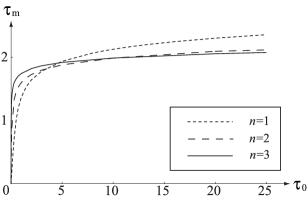
Figure 1: $\tau_{0}$ vs. $\tau_{{\rm m}}$. $n=1$ for dotted line, $n=2$ for dashed line, and $n=3$ for solid line.

Probably, there does not exist any static nonsingular monotonically-increasing D(F)-string solution of the tachyon equation (3.1) with $\tau(0)=0$ and $\tau(\infty)=\infty$. Since the aforementioned discussion does not rule out the singular solution $\tau$ with infinite slope $d\tau/dr\sim\infty$, the BPS solutions (2.18)–(2.19) are free from the argument of nonexistence. This conclusion, the nonexistence of regular static topological non-BPS D(F)-string solutions, is consistent with the same result of nonexistence in DBI EFT [17].

4 Conclusion

The system of D3${\bar{\rm D}}$3 has been considered in the scheme of super-BSFT EFT (2.1) including a complex tachyon and U(1)$\times$U(1) gauge fields. From the vanishing pressure difference, the first-order Bogomolnyi equation (2.15) was derived and straight topological BPS multi-D(F)-string configurations were given as exact static solutions (2.18)–(2.19) which also satisfy the conservation of energy-momentum tensor (2.9). Since the forms of derived Bogomolnyi equation and singular BPS solutions coincide exactly with those in DBI type EFT, this BPS structure seems universal and is consistent with type II superstring theories. The expression of energy was rewritten by the BPS sum rule for the BPS multi-D(F)-string solutions (2.25), and reproduced the descent relation for codimension-two objects (2.26), which allowed to interpret the obtained vortex-strings as BPS D1-branes in IIB string theory. This results in a constraint condition for the BPS tachyon potential (2.27), and the Gaussian type potential of BSFT (2.2) fulfills the condition. Since it is nothing but making a sum of delta functions in the thin BPS limit (2.28), the uniqueness of BPS tachyon potential seems unlikely. When the $z$-component of constant electric field (2.6) is turned on, the conjugate momentum of the gauge field, the charge density of fundamental strings (2.21), is confined along the D-strings. In addition, the corresponding Hamiltonian density takes a BPS formula (2.22), $\sqrt{p^{2}+q^{2}}$ form for the D1-charge density $q$ and the fundamental string charge density $p$, so that the configuration with constant electric field along the string direction is the DF-string (or $(p,q)$-string) from D3$\bar{\mathrm{D}}3$. Though we checked the conditions for BPS vortex configurations explicitly, the form of obtained BPS limit is different from the usual BPS bound for vortices, of which energy minimum is saturated only when the Bogomolnyi equations are satisfied. In this sense, the BPS bound for codimension-two branes from D${\bar{\rm D}}$ system needs further study. We also checked the possibility that the tachyon equation (3.1) could possess a nonsingular D(F)-string solutions and the analysis supported negative answer.

Since we achieved a BPS limit of multi-vortex-strings, it may open systematic study of classical dynamics of BPS multi-D(F)-strings, particularly moduli space dynamics in the context of BSFT. Studies of the D(F)-strings in curved spacetime naturally have cosmological implication as candidates of cosmic superstrings.

References

• [1] For a review, see A. Sen, “Tachyon dynamics in open string theory,” Int. J. Mod. Phys. A 20, 5513 (2005) [arXiv:hep-th/0410103], and references therein.
• [2] E. J. Copeland, R. C. Myers and J. Polchinski, “Cosmic F- and D-strings,” JHEP 0406, 013 (2004) [arXiv:hep-th/0312067].
• [3] G. Dvali and A. Vilenkin, “Formation and evolution of cosmic D-strings,” JCAP 0403, 010 (2004) [arXiv:hep-th/0312007].
• [4] E. B. Bogomolny, “Stability of classical solutions,” Sov. J. Nucl. Phys.  24, 449 (1976) [Yad. Fiz.  24, 861 (1976)].
• [5] For a review, see A. Vilenkin and E. P. S. Shellard, Cosmic strings and other topological defects, (Cambridge University Press, 1984) or T. W. B. Kibble, “Cosmic strings reborn?,” arXiv:astro-ph/0410073.
• [6] E. Witten, “On background independent open string field theory,” Phys. Rev. D 46, 5467 (1992) [arXiv:hep-th/9208027]; “Some computations in background independent off-shell string theory,” Phys. Rev. D 47, 3405 (1993) [arXiv:hep-th/9210065]; K. Li and E. Witten, “Role of short distance behavior in off-shell open string field theory,” Phys. Rev. D 48, 853 (1993) [arXiv:hep-th/9303067]; S. L. Shatashvili, “Comment on the background independent open string theory,” Phys. Lett. B 311, 83 (1993) [arXiv:hep-th/9303143], “On the problems with background independence in string theory,” Alg. Anal.  6, 215 (1994) [arXiv:hep-th/9311177].
• [7] A. A. Gerasimov and S. L. Shatashvili, “On exact tachyon potential in open string field theory,” JHEP 0010, 034 (2000) [arXiv:hep-th/0009103]; D. Kutasov, M. Marino and G. W. Moore, “Some exact results on tachyon condensation in string field theory,” JHEP 0010, 045 (2000) [arXiv:hep-th/0009148]; “Remarks on tachyon condensation in superstring field theory,” arXiv:hep-th/0010108.
• [8] P. Kraus and F. Larsen, “Boundary string field theory of the DD-bar system,” Phys. Rev. D 63, 106004 (2001) [arXiv:hep-th/0012198]; T. Takayanagi, S. Terashima and T. Uesugi, “Brane-antibrane action from boundary string field theory,” JHEP 0103, 019 (2001) [arXiv:hep-th/0012210].
• [9] N. T. Jones and S. H. H. Tye, “An improved brane anti-brane action from boundary superstring field theory and multi-vortex solutions,” JHEP 0301, 012 (2003) [arXiv:hep-th/0211180].
• [10] N. T. Jones, L. Leblond and S. H. H. Tye, “Adding a brane to the brane anti-brane action in BSFT,” JHEP 0310, 002 (2003) [arXiv:hep-th/0307086].
• [11] N. T. Jones and S. H. H. Tye, “Spectral flow and boundary string field theory for angled D-branes,” JHEP 0308, 037 (2003) [arXiv:hep-th/0307092].
• [12] K. Hashimoto and S. Hirano, “Metamorphosis of tachyon profile in unstable D9-branes,” Phys. Rev. D 65, 026006 (2002) [arXiv:hep-th/0102174].
• [13] S. Sugimoto and S. Terashima, “Tachyon matter in boundary string field theory,” JHEP 0207, 025 (2002) [arXiv:hep-th/0205085]; J. A. Minahan, “Rolling the tachyon in super BSFT,” JHEP 0207, 030 (2002) [arXiv:hep-th/0205098]; A. Ishida, Y. Kim and S. Kouwn, “Homogeneous rolling tachyons in boundary string field theory,” Phys. Lett.  B 638, 265 (2006) [arXiv:hep-th/0601208].
• [14] C. Kim, Y. Kim, O. K. Kwon and H. U. Yee, “Tachyon kinks in boundary string field theory,” JHEP 0603, 086 (2006) [arXiv:hep-th/0601206].
• [15] A. Sen, “Dirac-Born-Infeld action on the tachyon kink and vortex,” Phys. Rev. D 68, 066008 (2003) [arXiv:hep-th/0303057].
• [16] M. R. Garousi, “D-brane anti-D-brane effective action and brane interaction in open string channel,” JHEP 0501, 029 (2005) [arXiv:hep-th/0411222].
• [17] Y. Kim, B. Kyae and J. Lee, “Global and local D-vortices,” JHEP 0510, 002 (2005) [arXiv:hep-th/0508027]; I. Cho, Y. Kim and B. Kyae, “DF-strings from D3 D3-bar as cosmic strings,” JHEP 0604, 012 (2006) [arXiv:hep-th/0510218].
• [18] T. Kim, Y. Kim, B. Kyae and J. Lee, “Cosmic D- and DF-strings from D3D-bar3: Black strings and BPS bound,” arXiv:hep-th/0612285.
• [19] M. G. Jackson, N. T. Jones and J. Polchinski, “Collisions of cosmic F- and D-strings,” JHEP 0510, 013 (2005) [arXiv:hep-th/0405229]; A. Hanany and K. Hashimoto, “Reconnection of colliding cosmic strings,” JHEP 0506, 021 (2005) [arXiv:hep-th/0501031]; E. J. Copeland, T. W. B. Kibble and D. A. Steer, “Collisions of strings with Y junctions,” Phys. Rev. Lett.  97, 021602 (2006) [arXiv:hep-th/0601153]; “Constraints on string networks with junctions,” Phys. Rev.  D 75, 065024 (2007) [arXiv:hep-th/0611243].
• [20] S. H. Tye, I. Wasserman and M. Wyman, “Scaling of multi-tension cosmic superstring networks,” Phys. Rev. D 71, 103508 (2005) [Erratum-ibid. D 71, 129906 (2005)] [arXiv:astro-ph/0503506]; E. J. Copeland and P. M. Saffin, “On the evolution of cosmic-superstring networks,” JHEP 0511, 023 (2005) [arXiv:hep-th/0505110]; M. Hindmarsh and P. M. Saffin, “Scaling in a SU(2)/Z(3) model of cosmic superstring networks,” JHEP 0608, 066 (2006) [arXiv:hep-th/0605014].
• [21] H. Firouzjahi, L. Leblond and S. H. Henry Tye, “The (p,q) string tension in a warped deformed conifold,” JHEP 0605, 047 (2006) [arXiv:hep-th/0603161]; S. Thomas and J. Ward, “Non-Abelian (p,q) strings in the warped deformed conifold,” JHEP 0612, 057 (2006) [arXiv:hep-th/0605099].
• [22] M. Marino, “On the BV formulation of boundary superstring field theory,” JHEP 0106, 059 (2001) [arXiv:hep-th/0103089]; V. Niarchos and N. Prezas, “Boundary superstring field theory,” Nucl. Phys. B 619, 51 (2001) [arXiv:hep-th/0103102].
• [23] J. Hong, Y. Kim and P. Y. Pac, “On the multivortex solutions of the Abelian Chern-Simons-Higgs theory,” Phys. Rev. Lett.  64, 2230 (1990); R. Jackiw and E. J. Weinberg, “Selfdual Chern-Simons vortices,” Phys. Rev. Lett.  64, 2234 (1990).
• [24] L. C. Evans, Partial differential equations, (American Mathematical Society, Providence, 1998).
• [25] E. Witten, “Bound states of strings and p-branes,” Nucl. Phys.  B 460, 335 (1996) [arXiv:hep-th/9510135].