Instantons and Supersymmetry

Abstract

The role of instantons in describing non-perturbative aspects of globally supersymmetric gauge theories is reviewed. The cases of theories with ${\cal N}$=1, ${\cal N}$=2 and ${\cal N}$=4 supersymmetry are discussed. Special attention is devoted to the intriguing relation between instanton solutions in field theory and branes in string theory.

 
ROM2F/2007/08
TCDMATH 07–08
hep-th/0703142

1 Introduction

In this review we discuss the role of instantons in describing non-perturbative effects in globally supersymmetric gauge theories .

Instantons (anti-instantons) are non-trivial self-dual (anti-self-dual) solutions of the equations of motion of the pure non-abelian Yang–Mills theory when the latter is formulated in a compactified S₄ Euclidean manifold. Instanton solutions are characterised by a topological charge (the Pontrjagin number, $K$) which takes integer values, $K\in\mathbbm{Z}$. The integer $K$ represents the number of times the (sub)group $SU(2)$ of the gauge group is wrapped by the classical solution, while its space-time location spans the S₃-sphere at infinity.

The presentation of the material of this review can be naturally split into three parts according to the number of supersymmetries endowed by the theory. In the first part (Sects. 2-5) we discuss (weak and strong coupling) computations of instanton dominated correlators in pure ${\cal N}=1$ Super Yang–Mills (SYM) and in some Super QCD-like (SQCD) and chiral extensions of it. A careful analysis of the latter case shows that with a suitable choice of the chiral matter flavour representations the interesting phenomenon of dynamical breaking of supersymmetry occurs in the theory, as a consequence of the constraints imposed by the Konishi anomaly equation.

In the second part (Sects. 6-11) we move to the ${\cal N}=2$ Super Yang–Mills case. We will show how the highly sophisticated instanton calculus, developed in the years, is able to produce the correct coefficients that determine the exact expression of the ${\cal N}=2$ prepotential, derived in the famous Seiberg–Witten (SW) construction. We will also review the construction of the instanton solution in terms of branes with the purpose of illustrating the intriguing relation with string theory.

In the third part (Sects. 12-18) we discuss the role of instantons in ${\cal N}=4$ Super Yang–Mills. Although there are no anomalous $U(1)$’s in this theory (with the consequence that there exist no chiral $U(1)$ selection rules that would limit the value of Pontrjagin number of the instanton solutions contributing to correlators, as instead happens in the ${\cal N}=1$ and ${\cal N}=2$ cases), instantons are crucial to check the validity of the Maldacena conjecture beyond the realm of perturbation theory. Furthermore, their correspondence with IIB string D-instantons gives us hope to understand the yet elusive Montonen–Olive duality between the weak and strong coupling regimes of ${\cal N}=4$ Super Yang–Mills.

A detailed outline of this review is as follows. In Sect. 2 we start with some introductory remarks about instantons and their interpretation as field configurations interpolating between classical Euclidean vacua (quantum tunneling) and we discuss in detail how semi-classical calculations are performed in the instanton background with special reference to the notion of collective coordinates. We also illustrate the simplifications that occur in supersymmetric theories. In Sect. 3 we derive from supersymmetry and holomorphicity the general structure of the Green functions with only insertions of lowest (highest) components of chiral (anti-chiral) superfields. We show that these Green functions do not depend on the operator insertion points and have a completely fixed dependence upon the parameters of the theory (like masses and coupling constant). We then move in Sect. 4 to the explicit semi-classical instanton computation of constant Green functions in pure SYM and in massive SQCD finding perfect agreement between the theoretical expectations spelled out in the previous section and the results of actual calculations. The main result of this analysis is that the perturbative non-renormalisation theorems of supersymmetry are violated in the semi-classical instanton approximation. The instanton calculus is then extended to encompass the more delicate cases of massless SQCD and to Georgi–Glashow type theories with matter in suitable non-anomalous chiral representations. In the first case certain inconsistencies are found between results obtained in the massless limit of the massive theories and what can be directly computed in the strictly massless situation. The problem is discussed in detail and the issue of “strong coupling” vs “weak coupling” instanton calculation strategy is addressed. In the second case conflicting results with the constraints imposed by the Konishi anomaly equation lead to the conclusion that in certain supersymmetric chiral theories supersymmetry is dynamically broken by non-perturbative instanton effects. In Sect. 5 we give the expression of the effective action for all the cases for which we have obtained results in the semi-classical instanton approximation. A nice agreement between these two approaches is found, which gives support to instanton based computations.

We then pass to discuss instanton effects in ${\cal N}=2$ SYM theories. After the introduction to the subject contained in Sect. 6, we present some general discussion of their properties in Sect. 7. We start by recalling their supermultiplet content. We then describe the coupling of vector multiplets to hypermultiplets and the structure of the classical and effective actions. In Sect. 8 we review the celebrated analysis of Seiberg and Witten and the derivation of the expression of the analytic prepotential in the case of pure ${\cal N}=2$ SYM with $SU(2)$ gauge group. ${\cal N}=2$ instanton calculus is argued to provide a powerful check of the SW prepotential in Sect. 9. In Sect. 9.1 we describe Matone’s non-linear recursion relations for the expansion coefficients. The validity of the recursion relations and thus of the analytic prepotential itself is checked against instanton calculations for winding numbers $K=1$ and $K=2$ in Sect. 9.2. In order to go beyond these two cases, we follow the strategy advocated by Nekrasov and collaborators which is based on the possibility of topologically twisting ${\cal N}=2$ SYM theories and turning on a non-commutative deformation that localises the integration over instanton moduli spaces. After reviewing the strategy in Sect. 10, we describe how to couple hypermultiplets in Sect. 10.1. We then sketch the mathematical arguments that lead to the localisation of the measure in Sect. 10.2 and the computation of the residues that allows a non-perturbative check of the correctness of the SW prepotential for arbitrary winding number in Sect. 10.3. In Sect. 11 we change gear and exploit the Veneziano model and D-branes in order to embed (supersymmetric) YM theories in string theory. In particular we outline the emergence of the ADHM data and the ADHM equations as a result of the introduction of lower dimensional D-branes in a given configuration with maximal ${\cal N}=4$ supersymmetry. Finally we describe in Sect. 11.1 the truncation to ${\cal N}=2$ supersymmetry and the derivation of the SW prepotential within this framework in Sect. 11.2.

In the final part of the review, starting in Sect. 12, we discuss instanton effects in ${\mathcal{N}}=4$ SYM, focussing in particular on the rôle of instantons in the context of the AdS/CFT correspondence. ${\mathcal{N}}=4$ SYM is the maximally extended (rigid) supersymmetric theory in four dimensions and is believed to be exactly conformally invariant at the quantum level. The main properties of the model are reviewed in Sect. 13. We give explicitly the form of the action and the supersymmetry transformations and we discuss the basic implications of conformal invariance on the physics of the theory, highlighting some of the features which make it special compared to the ${\mathcal{N}}=1$ and ${\mathcal{N}}=2$ theories considered in previous sections. General aspects of instanton calculus in ${\mathcal{N}}=4$ SYM are presented in Sect. 14. We describe the general strategy for the calculation of instanton contributions to correlation functions of gauge-invariant composite operators in the semi-classical approximation, emphasising again the essential differences with respect to the ${\mathcal{N}}=1$ and ${\mathcal{N}}=2$ cases. In Sect. 15 we focus on the case of the $SU(N_{c})$ gauge group, which is relevant for the AdS/CFT duality, and we discuss in detail the calculation of correlation functions in the one-instanton sector. We first construct a generating function which facilitates a systematic analysis of instanton contributions to gauge-invariant correlators and we then present some explicit examples. The generalisation of these results to multi-instanton sectors in the large-$N_{c}$ limit is briefly outlined in Sect. 16. At this point we change somewhat perspective and we move to a discussion of the remarkable gauge/gravity duality conjectured by Maldacena, explaining how instanton calculus allows to test its validity beyond perturbation theory. In Sect. 17 we recall the basic aspects of the duality which relates ${\mathcal{N}}=4$ SYM to type IIB superstring theory in an AdS${}_{5}\times S^{5}$ background. Instanton effects in ${\mathcal{N}}=4$ SYM are in correspondence with the effects of D-instantons in string theory. More precisely instanton contributions to correlators in ${\mathcal{N}}=4$ SYM are related to D-instanton induced scattering amplitudes in the AdS${}_{5}\times S^{5}$ string theory. In Sects. 18.1 and 18.2 we present the calculation of D-instanton contributions to the string amplitudes dual to the SYM correlation functions studied in Sect. 15. The remarkable agreement between gauge and string theory calculations provides a rather stringent test of the conjectured duality. Finally in Sect. 18.3 we review the rôle of instantons in a particularly interesting limit of the AdS/CFT correspondence, the so-called BMN limit, in which the gravity side of the correspondence is under a better quantitative control beyond the low-energy supergravity approximation. We show how instanton effects provide again important insights into the non-perturbative features of the duality.

Our notation and various technical details are discussed in a number of Appendices.

Given the pedagogic nature of this review we refrain from drawing any conclusion or present any speculation. In Sect. 19 we try, instead, to summarise the crucial contributions given by Gabriele to the subject both as the father of open string theory and as one of the deepest and most original investigators of the non-perturbative aspects of gauge theories. We thus simply list a few lines of research activity where Gabriele’s profound insight was precious to put existing problems in the correct perspective and help in solving them.

2 Generalities about instantons

Instantons (anti-instantons) are self-dual (${F}_{\mu\nu}=\tilde{F}_{\mu\nu}$, $\tilde{F}_{\mu\nu}=\frac{1}{2}\epsilon_{\mu\nu\rho\sigma}F_{\rho\sigma}$) (anti-self-dual, ${F}_{\mu\nu}=-\tilde{F}_{\mu\nu}$) solutions of the classical non-abelian Yang–Mills (YM) Euclidean equations of motion (e.o.m.) BEL ; GTH  . They are classified by a topological number, the Pontrjagin (or winding) number, $K\in\mathbbm{Z}$, which represents the number of times the (sub)group $SU(2)$ of the gauge group is wrapped by the classical solution, $A_{\mu}^{aI}(x)$, when $x$ spans the S₃-sphere at the infinity of the compactified S₄ Euclidean space-time . Homotopy theory shows, in fact, that the homotopically inequivalent mappings S${}_{3}\to SU(2)$ are classified by integers since $\Pi_{3}(SU(2))\sim\Pi_{3}({\rm S}_{3})=\mathbbm{Z}$ BOOK .

2.1 The geometry of instantons

In the Feynman gauge ($\partial_{\mu}A_{\mu}^{a}=0$) the explicit expression of the gauge instanton with winding number $K=1$ for the $SU(2)$ gauge group (to which case we now restrict) is

$$A_{\mu}^{aI}=\frac{2}{g}\bar{\eta}^{a}_{\mu\nu}\frac{(x-x_{0})_{\nu}}{(x-x_{0})^{2}}\frac{\rho^{2}}{(x-x_{0})^{2}+\rho^{2}}\,,$$ (1)

where $\bar{\eta}^{a}_{\mu\nu}$ are the ’t Hooft symbols GTH  . In (1) $x_{0}$ and $\rho$ are the so-called location and size of the instanton, respectively. They are not fixed by the YM classical e.o.m., neither is the orientation of the instanton gauge field in colour space. Consequently the derivatives of the instanton solution with respect to each one of these parameters (collective coordinates GS ) will give rise to zero modes of the operator associated with the quadratic fluctuations of the gauge field in the instanton background GTH ; BER ; YAF (see Appendix 21 for details).

The winding number of a gauge configuration can be expressed in terms of the associated field strength through the (gauge invariant) formula

$$K=\frac{g^{2}}{32\pi^{2}}\int{\rm d}^{4}x\,F^{a}_{\mu\nu}\tilde{F}^{a}_{\mu\nu}\,.$$ (2)

For the action of a self-dual (or anti-self-dual) instanton configuration one then gets

$$S^{I}=\frac{8\pi^{2}}{g^{2}}|K|\,.$$ (3)

The topological nature of (1) can be better enlightened by first recasting it in the form ($y\equiv x-x_{0}$)

$$A_{\mu}^{I}=\frac{i}{g}\frac{\rho^{2}}{y^{2}+\rho^{2}}\big{[}\Omega^{(1)\dagger}\partial_{\mu}\Omega^{(1)}\big{]}(y)\,,$$ (4)

where (see (535))

$$\big{[}\Omega^{(1)\dagger}\partial_{\mu}\Omega^{(1)}\big{]}(x)=-\bar{\sigma}_{\mu\nu}\frac{x_{\nu}}{\sqrt{x^{2}}}\,.$$ (5)

In the previous equations

$$\Omega^{(1)}(x)=\sigma_{\mu}\frac{x_{\mu}}{\sqrt{x^{2}}}$$ (6)

is a topologically non-trivial $SU(2)$ gauge transformation, since it does not tend to the group identity as $\sqrt{x^{2}}$ tends to infinity. To compute the winding number of the gauge configuration (4) it is convenient to gauge transform it by the transformation $\Omega^{(1)}$ itself. One gets in this way

$$(A_{\mu}^{I})^{N.S.}=\big{[}A_{\mu}^{I}\big{]}^{\Omega^{(1)}}=\frac{i}{g}\frac{y^{2}}{y^{2}+\rho^{2}}\big{[}\Omega^{(1)}\partial_{\mu}\Omega^{(1)\dagger}\big{]}(y)=$$

$$=-\frac{i}{g}\sigma_{\mu\nu}\frac{y_{\nu}}{\sqrt{y^{2}}}\frac{y^{2}}{y^{2}+\rho^{2}}\,.$$ (7)

From the second equality we see that $(A_{\mu}^{I})^{N.S.}$ tends at infinity to a non-trivial pure gauge. Inserting (7) in (2), one gets the expected result, $K=1$.

The form (1) (or (4)) of the one-instanton field is called “singular” because the point where the non-vanishing contribution to the action integral comes from is at $x=x_{0}$, unlike the “non-singular” form (7) in which this point has been brought to infinity.

We recall in this context that the $F^{a}_{\mu\nu}\tilde{F}^{a}_{\mu\nu}$ density can be locally rewritten as the divergence of a gauge non-invariant vector through the formula

$$F^{a}_{\mu\nu}\tilde{F}^{a}_{\mu\nu}=2\partial_{\mu}K_{\mu}\,,\qquad K_{\mu}=\epsilon_{\mu\nu\rho\sigma}{\rm Tr}\big{[}A_{\nu}F_{\rho\sigma}+\frac{2ig}{3}A_{\nu}A_{\rho}A_{\sigma}\big{]}\,.$$ (8)

Thus (2) can be written

$$K=\frac{g^{2}}{16\pi^{2}}\int_{{\rm S}_{3}^{\infty}}{\rm d}S_{\mu}K_{\mu}\,,$$ (9)

where S${}_{3}^{\infty}$ is the three-sphere at infinity in S₄. Since, as we noticed above, $(A_{\mu}^{I})^{N.S.}$ tends to a pure gauge at infinity and hence its field strength vanishes, (9) can be cast in the very expressive form

$$K=\frac{1}{24\pi^{2}}\int_{{\rm S}_{3}^{\infty}}{\rm d}S_{\mu}\epsilon_{\mu\nu\rho\sigma}{\rm Tr}\big{[}\Omega^{\dagger}\partial_{\nu}\,\Omega\Omega^{\dagger}\partial_{\rho}\Omega\,\Omega^{\dagger}\partial_{\sigma}\Omega\big{]}\,,$$ (10)

in which we recognise the Cartan–Maurer formula. In general terms this quantity is an integer, which represents the winding number of the $SU(2)$ gauge transformation, $\Omega$ .

2.2 Quantum tunneling

The existence of instanton solutions in YM can be interpreted as an indication of quantum tunneling between different vacua, the latter being pure gauge configurations characterised by their winding numbers GTH ; TUN1 ; TUN2 . This fact can be illustrated in quite a number of ways. An easy, but heuristic argument is described below. A more sophisticated analysis is presented in Appendix 22.

Consider again the asymptotic formula (9), in which, however, the closed surface S${}_{3}^{\infty}$ has been (smoothly) deformed to an other closed surface, which we take as a hyper-cylinder of length $T$, bounded at $t=-T/2$ and $t=T/2$ by three-dimensional compact spatial manifolds, S₃. In the limit $T\to\infty$ (9) can then be rewritten as the sum of three contributions

$$K=\frac{ig^{3}}{24\pi^{2}}\lim_{T\to\infty}\Big{(}\int_{{\rm S}_{3}}{\rm d}^{3}x\,\epsilon_{4ijk}{\rm Tr}\big{[}A_{i}A_{j}A_{k}\big{]}|_{t=T/2}+$$

$$-\int_{{\rm S}_{3}}{\rm d}^{3}x\,\epsilon_{4ijk}{\rm Tr}\big{[}A_{i}A_{j}A_{k}\big{]}|_{t=-T/2}+$$

$$+\int_{-T/2}^{T/2}\int_{{\rm S}_{L}}{\rm d}S_{i}\,\epsilon_{i\nu\rho\sigma}{\rm Tr}\big{[}A_{\nu}A_{\rho}A_{\sigma}\big{]}\Big{)}\,,$$ (11)

where ${\rm S}_{L}$ is the three-dimensional lateral surface of the cylinder. It can be proved SCIU that one can always find a gauge where 1) $A_{0}=0$ on the lateral surface ${\rm S}_{L}$; 2) the (time-independent) gauge transformations $\Omega_{\pm}(\vec{x})$ at $t=\pm T/2$ are such that at large $|\vec{x}|$ they are independent on the direction $\vec{x}/|\vec{x}|$. Under these conditions the third term in the r.h.s. of (11) vanishes. The other two terms take integer values because they represent the winding number of the mapping $\vec{x}\to\Omega_{\pm}(\vec{x})$ from the (manifold $\mathbbm{R}^{3}$ compactified to the) S₃ sphere onto $SU(2)$ . The net result of these considerations is that (11) can be cast in the form

$$K=n_{+}-n_{-}\,,$$ (12)

$$n_{\pm}=-\frac{1}{24\pi^{2}}\epsilon_{ijk}\int_{{\rm S}_{3}}{\rm d}^{3}x\,{\rm Tr}\big{[}\Omega^{\dagger}_{\pm}\partial_{i}\Omega_{\pm}\,\Omega^{\dagger}_{\pm}\partial_{j}\Omega_{\pm}\,\Omega^{\dagger}_{\pm}\partial_{k}\Omega_{\pm}(\vec{x})\big{]}\,,$$ (13)

which shows that the instanton solution ($K\neq 0$) interpolates between vacuum states (pure gauge configurations) with different winding numbers.

We refer the reader to Appendix 22 for a more rigorous discussion of instanton induced tunneling effects in a YM theory.

2.3 Introducing fermions

In this subsection we want to briefly recall some elementary facts on how to deal with fermions in the functional language in general and in the semi-classical approximation in particular.

Fermionic functional integration

When fermions are introduced it is necessary to define integration rules for Grassmann variables. This is a beautiful piece of mathematics of which a simple account can be found in BERE . The well-known results of this analysis can be summarised as follows.

1) The functional integration over the degrees of freedom of a Dirac fermion belonging to the representation ${\bf R}$ of the gauge group has the effect of adding to the gauge action a contribution which is formally given by

$$\log\left\{\int{\cal D}\mu[{\bf R}](\psi,\bar{\psi})\exp\big{[}\int{\rm d}^{4}x\,(\bar{\psi}i\gamma_{\mu}D_{\mu}[{\bf R}]\psi)(x)\big{]}\right\}=$$

$$=\log\left\{{\rm det}\big{[}i\gamma_{\mu}D_{\mu}[{\bf R}]\big{]}\right\}={\rm Tr}\log\big{[}i\gamma_{\mu}D_{\mu}[{\bf R}]\big{]}\,,$$ (14)

where

$$iD_{\mu}[{\bf R}]\gamma_{\mu}=iD_{\mu}[{\bf R}]\left(\begin{array}[]{cc}0&\sigma_{\mu}\\ \bar{\sigma}_{\mu}&0\end{array}\right)$$ (15)

and the matrices $\sigma_{\mu}$ and $\bar{\sigma}_{\mu}$ are defined in Appendix 20.

2) For a Weyl fermion, which has half the degrees of freedom of a Dirac fermion (compare (15) and (533)), there is the subtlety that the Dirac–Weyl operator maps dotted indices into undotted ones, thus making problematic the definition of a determinant for such an operator. In the literature many prescriptions have been proposed to address this issue in a rigorous way (see MEU and works quoted therein). Actually this difficulty is not relevant in practice, because one can always imagine to factor out the free operator and compute the determinant of the resulting operator which is perfectly well defined MRT . The contribution from the free part is obviously irrelevant in the computation of Green functions as it will cancel with an identical contribution from the normalisation factor (see (522)). Loosely speaking, looking at (15) and (533), we may say that ceteris paribus the contribution of a Weyl fermion to the functional integral is the “square root” of that of a Dirac fermion.

Fermionic zero modes

In computing the fermionic functional integral one is led to consider the decomposition of the associated spinor fields in eigenstates of the fermionic kinetic operator. As is well known, the existence of zero modes in certain background gauge fields, such as instantons, is of particular relevance for non-perturbative calculations both in ordinary and supersymmetric field theories GTH ; AKMRV ; REV .

The number of zero modes of the Dirac operator in an external field is controlled by the famous Atiyah-Singer index theorem AS . The theorem states that “the index of the Dirac operator (15), i.e. the difference between the number of left-handed ($n_{L}$) and right-handed ($n_{R}$) zero modes, is equal to twice the Dynkin index of the representation ${\bf R}$ times the Pontrjagin number of the background gauge field”. In formulae we write

$${\rm ind}(D_{\mu}[{\bf R}]\gamma_{\mu})\equiv n_{L}-n_{R}=2\ell[{\bf R}]K\,,$$ (16)

where $\ell[{\bf R}]$ is the Dynkin index of the representation ${\bf R}$. Let us now consider some interesting applications of this theorem.

1. Weyl fermion in the adjoint representation, ${\bf Adj}$, of the gauge group. We must distinguish between the left-handed ($D_{\mu}[{\bf Adj}]\bar{\sigma}_{\mu}$) and the right-handed ($D_{\mu}[{\bf Adj}]\sigma_{\mu}$) Weyl operator. In the first case $n_{R}=0$ and the formula (16) becomes

   $${\rm ind}(D_{\mu}[{\bf Adj}]\bar{\sigma}_{\mu})=n_{L}=2N_{c}K\,,$$ (17)

   because $\ell[{\bf Adj}]=N_{c}$. Since obviously $n_{L}$ is a non-negative number, there can exist zero modes of the left-handed Weyl operator only if the classical background instanton field has positive winding number, $K>0$. Similarly for the right-handed Weyl operator one gets

   $${\rm ind}(D_{\mu}[{\bf Adj}]\sigma_{\mu})=-n_{R}=2N_{c}K\,,$$ (18)

   implying that there can be zero modes only if $K<0$.

2. Actually the number of zero-modes in the adjoint representation of any compact Lie group, $G$, is always given by twice the value of the quadratic Casimir operator, $2c_{2}({\bf Adj}(G))$. This result follows from the formula BCGW

   $${\bf Adj}(G)=4{\bf Adj}(SU(2))+n(G)\,{\bf 2}+s(G)\,{\bf 1}\,,$$ (19)

   which expresses how the adjoint representation of $G$ can be decomposed into irreducible representations of $SU(2)$. In (19) we have introduced the definitions

   $$n(G)=2(c_{2}({\bf Adj}(G))-2)\,,$$ (20)

   $$s(G)=d({\bf Adj}(G))-4c_{2}({\bf Adj}(G))+5\,,$$ (21)

   where $d({\bf Adj}(G))$ is the dimension of the adjoint representation of $G$. The number of zero-modes is then $4+2(c_{2}({\bf Adj}(G))-2)=2c_{2}({\bf Adj}(G))$

3. Dirac fermion in the fundamental representation, ${\bf N_{c}}$, of the gauge group. Equation (16) with $\ell[{\bf N_{c}}]=1/2$ gives

   $${\rm ind}(D_{\mu}[{\bf N_{c}}]\gamma_{\mu})=n_{L}-n_{R}=K\,.$$ (22)

   Again in the classical background instanton field there can be either left-handed fermionic zero modes, if $K>0$, or right-handed ones, if $K<0$.

4. Fermion in the rank-two antisymmetric representation ${\bf N_{c}(N_{c}-1)/2}$. The number of zero modes (of definite chirality) is $(N_{c}-2)K$.

Deriving the explicit expression of all these fermionic zero modes is beyond the scope of this review and we refer the interested reader to the general methods that, starting from the seminal paper of ADHM , have been developed in the literature TEM ; KHOREV . However, for completeness we give their explicit expression for a few cases more relevant for this review in Appendix 20.

2.4 Putting together fermion and boson contributions

As we said, we are interested in computing expectation values of (multi-local) gauge invariant operators, by dominating the functional integral with the semi-classical contributions coming from the non-trivial minima (instantons) of the Euclidean action. The obvious question is whether this computational strategy leads to a reliable estimate of $\langle O\rangle$.

The general case

In order to prepare ourselves for this analysis, let us write down the formal result obtained by performing the integration over the quadratic fluctuations (semi-classical approximation, s.c.) around an instanton solution with winding number $K$. Including also the fermionic contribution in (578) and assuming for simplicity that there are no scalar fields in the theory , one gets

$$\langle O\rangle\Big{|}_{s.c.}=\mu^{n_{B}-\kappa_{F}n_{F}}\frac{{\rm e}^{-\frac{8\pi^{2}}{g^{2}}|K|}}{Z|_{s.c.}}$$ (23)

$$\int\!\prod_{j=1}^{n_{F}}{\rm d}c_{j}\int\!\prod_{i=1}^{n_{B}}{\rm d}\beta_{i}\frac{||a^{(i)}||}{\sqrt{2\pi}}\frac{({\rm det}^{\prime}[{\cal M}_{\mu\nu}^{g.f.}])^{-\frac{1}{2}}{\rm det}[-D^{2}(A^{I})]}{({\rm det}[{\cal M}_{0;\mu\nu}^{g.f.}])^{-\frac{1}{2}}{\rm det}[-\partial^{2}]}\frac{{\rm det}^{\prime}[{\mbox{$\not\!\!D$}}(A^{I})]}{{\rm det}[\,\mbox{$\not\!\!\partial$}\,]}\,O(c;A^{I})\,.$$

where $\not\!\!D$ is the fermionic kinetic operator appropriate to the kind of fermion one is dealing with (Dirac or Weyl) and the prime on the determinants is there to mean that obviously only non-zero eigenvalues are to be included. Further observations about this formula are the following.

$\bullet$ The factor $\kappa_{F}$ is 1 for a Dirac fermion and $\frac{1}{2}$ for a Weyl fermion.

$\bullet$ The residual fermionic integration $\prod_{j=1}^{n_{F}}dc_{j}$ is over the Grassmannian coefficients associated with the $n_{F}$ zero modes of the fermionic kinetic operator. We stress that in order not to get a trivially vanishing result, the Berezin BERE integration rules require a perfect matching in the number of fermionic zero modes between those of the fermion operators in the action and those contained in the operator $O$.

$\bullet$ The extra $\mu$ dependence in front of the r.h.s. of (23) (with respect to (578)) is due (similarly to the case of the bosonic functional integration, see Appendix 21), to unmatched $\mu$ factors coming from the determinant of the fermion Pauli–Villars (PV) regulators .

$\bullet$ The power $\kappa_{F}n_{F}$ is dictated by the way in which zero modes contribute to the fermionic mass term in the action and the nature of the Grassmannian integration rules.

$\bullet$ No further factor comes from dealing with the fermionic zero modes, provided they are normalised to one, which we will always do (this is at variance with what happens for bosonic zero modes, each of which contributes a factor $||{\rm norm}||/\sqrt{2\pi}$ to (23)).

$\bullet$ Generally speaking, the ratio of determinants in (23) will be a function of the instanton collective coordinates as well as $\mu$.

The computational strategy outlined above can be safely used if it can be convincingly argued that the classical minima (instantons) really dominate the integral. This is a delicate issue which can only be settled on a case by case basis. For instance, for the instanton contribution to dominate the functional integral one can imagine considering Green functions that are zero in perturbation theory. The argument here is that otherwise the non-perturbative instanton contribution, which is proportional to $\exp(-{8\pi^{2}}|K|/{g^{2}})$, would represent a completely negligible correction with respect to any perturbative term. This is the situation one is usually dealing with in ${\cal N}=1$ supersymmetric theories.

In the ${\cal N}=2$ and ${\cal N}=4$ cases it is, instead, interesting to consider more general correlators which do not necessarily vanish in perturbation theory. In these cases instanton contributions, though comparatively exponentially small, can always be “tracked” if the theory $\vartheta$-dependence is followed (see Appendix 22).

A second crucial question concerns the finiteness of the r.h.s. of (23). In his beautiful paper ’t Hooft GTH has shown that in QCD the integration over the instanton collective coordinates around the classical instanton solution

$$A_{\mu}=A^{I}_{\mu}\,,\qquad{\rm all\,\,other\,\,fields\,\,equal\,to\,\,zero}$$ (24)

does not lead to a finite result. The reason behind this fact is that the integration over the size of the instanton, $\rho$, which comes from the ratios of determinant in (23) as well as from the norm of the bosonic zero modes, diverges in the infrared limit, i.e. for large values of $\rho$ (the integration near $\rho=0$ is, instead, convergent thanks to asymptotic freedom). This problem is not present in the supersymmetric case which we discuss next.

The supersymmetric case

Something really surprising indeed happens in the case of a supersymmetric theory. There, irrespective of the details of the theory (number of supersymmetries, gauge group, matter content, etc.), the whole ratio of (regularised) determinants is always exactly equal to 1 DADI . This is because the eigenvalues of the various kinetic operators in the instanton background are, up to multiplicities, essentially all equal and, due to supersymmetry, there is a perfect matching between bosonic and fermionic degrees of freedom, leading to contributions that are one the inverse of the other. The formula (23) thus becomes

$$\langle O\rangle\Big{|}_{s.c.}^{\rm SUSY}=\mu^{n_{B}-\frac{1}{2}n_{F}}\frac{{\rm e}^{-\frac{8\pi^{2}}{g^{2}}|K|}}{Z|_{s.c.}}\times$$

$$\times\int\prod_{i=1}^{n_{B}}{\rm d}\beta_{i}\frac{||a^{(i)}||}{\sqrt{2\pi}}\sum_{\{j_{k}\}}(-1)^{P_{\{j_{k}\}}}O(\prod_{k}f_{j_{k}};A^{I})\,,$$ (25)

where we have explicitly carried out the final integration over the Grassmannian variables $c_{j}$, ${j=1,2,\ldots,n_{F}}$. As a result the product of the $n_{F}$ fermionic fields contained in $O$ is simply replaced by the product of the wave functions, $f_{j}(x,\beta)$, of the $n_{F}$ zero modes. The sum over permutations is weighted by alternating signs because of Fermi statistics. Finally we have set $\kappa_{F}=\frac{1}{2}$, because in supersymmetric theories fermions are always introduced as Weyl particles.

Actually in the case $K=1$ (25) can be made even more explicit, because for a gauge invariant operator the only dependence on the collective coordinates is that on the size and position of the instanton. Using (584) of Appendix 21 and the coset integration formula (derived in BER ) necessary for the generalisation to the case of the $SU(N_{c})$ group, one gets to leading order in $g$ (where $Z|_{s.c.}=1$)

$$\langle O\rangle\Big{|}_{s.c.}^{\rm SUSY}=V_{N_{c}}\mu^{4N_{c}-\frac{1}{2}n_{F}}\frac{{\rm e}^{-\frac{8\pi^{2}}{g^{2}}}}{(g^{2})^{2N_{c}}}\times$$

$$\times\int\!\frac{{\rm d}\rho}{\rho^{5}}\,{\rm d}^{4}x_{0}(\rho^{2})^{2N_{c}}\sum_{\{j_{k}\}}(-1)^{P_{\{j_{k}\}}}O(\prod_{k}f_{j_{k}};A^{I})\,,$$ (26)

with

$$V_{N_{c}}=\frac{4}{\pi^{2}}\frac{(4\pi^{2})^{2N_{c}}}{(N_{c}-1)!(N_{c}-2)!}\,.$$ (27)

Supersymmetry has in store another surprise for us. Recalling the multiplicity of the fermionic zero modes as given by the Atiyah–Singer theorem (see Appendix 20), one finds that for a supersymmetric theory

$$4N_{c}-\frac{1}{2}n_{F}=b_{1}\,,$$ (28)

$$\beta=-\frac{g^{3}}{16\pi^{2}}b_{1}+{\rm O}(g^{5})\,,$$ (29)

where $b_{1}>0$ is the first coefficient of the Callan–Symanzik $\beta$-function. To prove (28) we recall the general formula

$$b_{1}=\frac{11}{3}\ell[{\bf Adj}]-\frac{2}{3}\sum_{{\bf R_{F}}}n_{{\bf R_{F}}}\ell[{\bf R_{F}}]-\frac{1}{3}\sum_{{\bf R_{B}}}n_{{\bf R_{B}}}\ell[{\bf R_{B}}]\,,$$ (30)

where $n_{{\bf R_{F}}}$ and $n_{{\bf R_{B}}}$ are the numbers of fermions and bosons in the representations ${\bf R_{F}}$ and ${\bf R_{B}}$, respectively. Since in a supersymmetric theory each fermion is accompanied by a bosonic partner belonging to the same representation ${\bf R}$, (30) simplifies to

$$b_{1}=3\ell[{\bf Adj}]-\sum_{{\bf R}}n_{{\bf R}}\ell[{\bf R}]=3N_{c}-\sum_{{\bf R}}n_{{\bf R}}\ell[{\bf R}]\,,$$ (31)

with $n_{{\bf R}}$ the number of chiral superfields in the representation ${\bf R}$. To be able to compare $b_{1}$ in the above equation with the combination that appears in the l.h.s. of (28) we make use of the Atiyah–Singer theorem (see (16)). Separating out the contribution due to gluinos (the fermions in the gauge supermultiplet) which accounts for a $2N_{c}/2$ contribution, we can write the l.h.s. of (28) in the form

$$4N_{c}-\frac{1}{2}n_{F}=4N_{c}-N_{c}-\frac{1}{2}2\sum_{{\bf R}}n_{{\bf R}}\ell[{\bf R}]=3N_{c}-\sum_{{\bf R}}n_{{\bf R}}\ell[{\bf R}]\,,$$ (32)

in agreement with (31).

The interesting consequence of this equality is that we can combine the exponential of the instanton action with the explicit $\mu$ dependence to form the renormalisation group invariant $\Lambda$-parameter of the theory. Introducing the running coupling $g(\mu)$, we can thus write

$$\mu^{4N_{c}-\frac{1}{2}n_{F}}{\rm e}^{-\frac{8\pi^{2}}{g(\mu)^{2}}}=\Lambda^{b_{1}}\,.$$ (33)

We will exploit this key observation in the following, making it more precise (Sect. 4.1).

3 Chiral and supersymmetric Ward–Takahashi identities

Before embarking in explicit instantonic calculations of correlators, we want to spell out the constraints imposed on correlators by chiral and supersymmetric Ward–Takahashi identities (WTI’s). We will show that in some interesting cases, when these “geometric” constraints are coupled to the requirement of renormalisability, the expression of certain Green functions is (up to multiplicative numerical constants) completely fixed.

The special Green functions which enjoy this amazing property are the $n$-point correlation functions of lowest (highest) components of chiral (anti-chiral) gauge invariant composite superfields. Although this is a very limited set of correlators, we will see that their knowledge, when used in conjunction with clustering, is sufficient to draw interesting non-perturbative information about the structure of the vacuum and of its symmetry properties. For this reason in this section we will limit our consideration to such correlators. We will in particular concentrate on the case of ${\cal N}=1$ Super QCD (SQCD) (see Appendix 20 for notations) with the purpose of exploring the properties of a sufficiently general theory in which also mass terms can be present.

WTI’s provide relations among different Green functions. They will be worked out under the assumption that supersymmetry is not spontaneously (or explicitly) broken, i.e. under the assumption that the vacuum of the theory is annihilated by all the generators of supersymmetry. Our philosophy will be that, if we find that some dynamical calculation turns out to be in contradiction with constraints imposed by supersymmetry, then this should be interpreted as evidence for spontaneous supersymmetry breaking.

As we explained above, we are now going to consider the $n$-point Green functions

$$G(x_{1},\ldots,x_{n})=\langle 0|T\big{(}\chi_{1}(x_{1})\ldots\chi_{n}(x_{n})\big{)})|0\rangle\,,$$ (34)

where each $\chi_{k}(x_{k})$ is a local gauge invariant operator made out of a products of lowest components of the fundamental chiral superfields of the theory. Thus the operators $\chi_{k}$ are themselves lowest components of some composite chiral super field, $X_{k}$, for which we formally have the expansion

$$X_{k}(x)=\chi_{k}(y)+\sqrt{2}\theta^{\alpha}\psi_{\alpha k}(y)+\theta^{2}F_{k}(y)\,,$$ (35)

$$y_{\mu}=x_{\mu}+i\theta^{\alpha}\sigma_{\mu}^{\alpha\dot{\alpha}}\bar{\theta}_{\dot{\alpha}}\,.$$ (36)

On these fields the $Q$ and $\bar{Q}$ generators of supersymmetry act as “raising” and “lowering” operators according to the (anti-)commutation rules

$$[\bar{Q}^{\dot{\alpha}},\chi_{k}(x)]=0\,,\qquad \{\bar{Q}^{\dot{\alpha}},\psi^{\alpha}_{k}(x)\}=\sqrt{2}\,\bar{\sigma}_{\mu}^{\dot{\alpha}\alpha}\partial_{\mu}\chi_{k}(x)\,,$$ (37)

$$[Q_{\alpha},F_{k}(x)]=0\,,\qquad \{Q_{\alpha},\psi_{k\beta}(x)\}=\sqrt{2}\epsilon_{\alpha\beta}F_{k}(x)\,.$$ (38)

3.1 Space-time dependence

The independence of the correlators of the form (34) from space-time arguments immediately follows from the (anti-)commutation relations (37). Taking, in fact, the derivative of $G$ with respect to $x_{\ell}$ and contracting with $\sqrt{2}\,\bar{\sigma}_{\mu}^{\dot{\alpha}\alpha}$, one gets

$$\sqrt{2}\,\bar{\sigma}_{\mu}^{\dot{\alpha}\alpha}\frac{\partial}{\partial x_{\ell\mu}}G(x_{1},\ldots,x_{n})=$$

$$=\langle 0|T\big{(}\chi_{1}(x_{1})\ldots\{\bar{Q}^{\dot{\alpha}},\psi^{\alpha}_{\ell}(x_{\ell})\}\ldots\chi_{n}(x_{n})\big{)}|0\rangle=0\,.$$ (39)

The last equality is a consequence of the fact that $\bar{Q}$ can be freely (first commutation rule in (37)) brought to act on the vacuum state at the beginning and at the end of the string of $\chi_{k}$ operators and that, under the assumption that supersymmetry is unbroken, $\bar{Q}|0\rangle=0$. Contributions coming from the derivative acting on the $\theta$-functions that prescribe the time-ordering of operators in $G$ are zero because they give rise to the vanishing equal-time commutators, $[\chi_{\ell}(\vec{x}_{\ell},t_{\ell}),\chi_{k}(\vec{x}_{k},t_{k})]\delta(t_{k}-t_{\ell})=0$. Equation (39) proves the constancy of $G$. A similar result clearly holds for $n$-point correlators, $G^{*}$, where only lowest components of antichiral superfields are inserted.

We end this section with the important observation that all these correlators vanish identically in perturbation theory. Only non-perturbative instanton-like contributions can make them non-zero.

3.2 Mass and $g$ dependence

The following further properties hold for correlators of lowest components of chiral, $G$, (or antichiral, $G^{*}$) superfields SWTI1 ; ARV ; AKMRV

a) $G$ is an analytic function of the complex mass parameters $m_{f}$, i.e. it does not depend on $m_{f}^{*}$ (the opposite being true for $G^{*}$).

b) The mass dependence of $G$ (and $G^{*}$) is completely fixed.

c) When renormalisation group invariant operators are inserted, the dependence upon the coupling constant is, in a mass independent renormalisation scheme, fully accounted for by the renormalisation group invariant (RGI) quantities $\Lambda$ and $[m_{f}]_{\rm inv}\equiv\hat{m}_{f}$ (see below (51)).

It is important to remark that properties of this kind can be readily exported to the generating functional of Green functions, as they only follow from symmetry principles. They provide strong constraints on the form of the associated effective action. A celebrated example of application of this observation, though in a different context, can be found in the construction of the low energy effective action that describes the interaction of pions in QCD WEIN ; GL . In supersymmetric theories the invariances are so tight that often the full expression of the effective superpotential is completely determined VY ; TVY ; ADSALL1 ; ADSALL2 (see Sect. 5).

a) Mass analyticity

The statement a) follows from the supersymmetric relation (no sum over $f$)

$$m^{*}_{f}\frac{\partial}{\partial m^{*}_{f}}G(x_{1},\ldots,x_{n})=m^{*}_{f}\langle 0|T\big{(}\chi_{1}(x_{1}),\ldots,\chi_{n}(x_{n})\int{\rm d}^{4}x\,F^{*f}_{f}(x)\big{)}|0\rangle=$$

$$=m^{*}_{f}\int{\rm d}^{4}x\,\langle 0|T\big{(}\chi_{1}(x_{1})\ldots\chi_{n}(x_{n})\{\bar{Q}_{\dot{\alpha}}\psi^{f\dot{\alpha}}_{f}(x)\}\big{)}|0\rangle=0\,,$$ (40)

with $F^{*f}_{f}$ the auxiliary field of the antichiral superfield $T^{*f}_{f}=(\chi^{*f}_{f},\bar{\psi}^{*f}_{f},F^{*f}_{f})$. The first equality follows from the fact that, before the auxiliary field is eliminated by the e.o.m., $F^{*f}_{f}$ is the coefficient of $m^{*}_{f}$. The second is a consequence of the complex conjugate of the anticommutation relation in (38). Finally, since $\bar{Q}$ commutes with the $\chi_{k}$’s, it can be brought in contact with the vacuum state which is thus annihilated.

b) Mass dependence

In order to simplify this analysis we restrict to Green functions where only the gauge invariant composite operators

$$\frac{g^{2}}{32\pi^{2}}\lambda^{\alpha a}(x)\lambda_{\alpha}^{a}(x)\equiv\frac{g^{2}}{32\pi^{2}}\lambda\lambda(x)\,,$$ (41)

$$\tilde{\phi}^{fr}(x)\phi_{hr}(x)\equiv\tilde{\phi}^{f}\phi_{h}(x)$$ (42)

are inserted. They are the lowest components of chiral superfields which will be called $S$ and $T^{f}_{h}$, respectively. Besides their obvious complex conjugate fields, we will sometimes also consider the composite operators $\tilde{\psi}^{fr}_{\alpha}(x)\psi^{\alpha}_{hr}(x)=\tilde{\psi}^{f}\psi_{h}(x)$. In general terms we will consider correlators of the kind

$$G^{(p,q)f_{1},\ldots,f_{p}}_{h_{1},\ldots,h_{p}}(x_{1},\ldots,x_{p};x_{p+1},\ldots,x_{p+q})=$$ (43)

$$=\langle 0|T\big{(}\tilde{\phi}^{f_{1}}\phi_{h_{1}}(x_{1})\ldots\tilde{\phi}^{f_{p}}\phi_{h_{p}}(x_{p})\frac{g^{2}}{32\pi^{2}}\lambda\lambda(x_{p+1})\ldots\frac{g^{2}}{32\pi^{2}}\lambda\lambda(x_{p+q})\big{)})|0\rangle\,.$$

The dependence of (43) upon the mass parameters can be established in the following way. First of all we notice that from (40) we have

$$m_{f}\frac{\partial}{\partial m_{f}}\,G^{(p,q)}=\Big{(}m_{f}\frac{\partial}{\partial m_{f}}-m^{*}_{f}\frac{\partial}{\partial m^{*}_{f}}\Big{)\,}G^{(p,q)}=\frac{1}{i}\frac{\partial}{\partial\alpha_{f}}\,G^{(p,q)}\,,$$ (44)

where we have set

$$m_{f}=|m_{f}|{\rm e}^{i\alpha_{f}}\,.$$ (45)

In order to compute the derivative in the r.h.s. of (44) we perform the non-anomalous $U_{A}^{f}(1)$ transformation (see Appendix 20)

$$(\tilde{\psi}^{h},\psi_{h})\to{\rm e}^{i\delta_{fh}\alpha_{f}/2}(\tilde{\psi}^{h},\psi_{h})\,,\quad(\tilde{\phi}^{h},\psi_{h})\to{\rm e}^{i(\delta_{fh}-1/N_{c})\alpha_{f}/2}(\tilde{\phi}^{h},\psi_{h})\,,$$

$$\lambda\to{\rm e}^{-i\alpha_{f}/2N_{c}}\lambda\,,$$ (46)

by means of which the $\alpha_{f}$ dependence of the action is eliminated, but it is brought in the fields appearing in $G^{(p,q)}$. This allows to carry out in an explicit way the $\alpha_{f}$ derivative, leading to the result

$$m_{f}\frac{\partial}{\partial m_{f}}G^{(p,q)f_{1},\ldots,f_{p}}_{h_{1},\ldots,h_{p}}=q^{(f),f_{1},\ldots,f_{p}}_{h_{1},\ldots,h_{p}}G^{(p,q)f_{1},\ldots,f_{p}}_{h_{1},\ldots,h_{p}}\,,$$ (47)

$$q^{(f),f_{1},\ldots,f_{p}}_{h_{1},\ldots,h_{p}}=\frac{p+q}{N_{c}}-\frac{1}{2}\sum_{\ell=1}^{p}(\delta_{f_{\ell},f}+\delta_{h_{\ell},f})\,,$$ (48)

where $q^{(f)}$ is the sum of all the $U_{A}^{f}(1)$ charges of the operators contained in $G^{(p,q)}$. The above differential equation is easily integrated and yields

$$\prod_{\ell=1}^{p}(m_{f_{\ell}}m_{h_{\ell}})^{\frac{1}{2}}G^{(p,q)f_{1},\ldots,f_{p}}_{h_{1},\ldots,h_{p}}=C^{(p,q)f_{1},\ldots,f_{p}}_{h_{1},\ldots,h_{p}}(\mu,g)\Big{(}\prod_{\ell=1}^{N_{f}}m_{\ell}\Big{)}^{\frac{(p+q)}{N_{c}}}\,.$$ (49)

The $\mu$ dependence of $C^{(p,q)f_{1},\ldots,f_{p}}_{h_{1},\ldots,h_{p}}(\mu,g)$ is trivially fixed by dimensional analysis and one finds

$$C^{(p,q)f_{1},\ldots,f_{p}}_{h_{1},\ldots,h_{p}}(\mu,g)\propto\mu^{(p+q)(3-N_{f}/N_{c})}\,.$$ (50)

c) $g$ dependence

The $g$ dependence of $C^{(p,q)f_{1},\ldots,f_{p}}_{h_{1},\ldots,h_{p}}(\mu,g)$ is completely determined by renormalisability. In fact, having factorised in the l.h.s. of (49) the mass factor $\prod_{\ell=1}^{p}(m_{f_{\ell}}m_{h_{\ell}})^{\frac{1}{2}}$, which precisely serves the purpose of making the $\tilde{\phi}^{f}\phi_{h}$ operators in $G^{(p,q)}$ behave like RGI insertions, the rest of the $g$ dependence must all be expressed through the RGI quantities

$$\Lambda=\mu\exp\Big{(}-\int^{g}\frac{1}{\beta(g^{\prime})}{\rm d}g^{\prime}\Big{)}\,,\quad\hat{m}=m\exp\Big{(}-\int^{g}\frac{\gamma_{m}(g^{\prime})}{\beta(g^{\prime})}{\rm d}g^{\prime}\Big{)}\,,$$ (51)

where $\beta\neq 0$ and $\gamma_{m}(g)$ are the Callan–Symanzik function of the theory and the mass anomalous dimension of the matter superfield, respectively. This implies that the $g$ dependence must be of the form

$$C^{(p,q)f_{1},\ldots,f_{p}}_{h_{1},\ldots,h_{p}}(\mu,g)\propto\exp\Big{\{}-\int^{g}\frac{{\rm d}g^{\prime}}{\beta(g^{\prime})}(p+q)\big{[}(3-\frac{N_{f}}{N_{c}})+\gamma_{m}(g^{\prime})\frac{N_{f}}{N_{c}}\big{]}\Big{\}}\,,$$ (52)

in order to have

$$\prod_{\ell=1}^{p}(m_{f_{\ell}}m_{h_{\ell}})^{\frac{1}{2}}G^{(p,q)f_{1},\ldots,f_{p}}_{h_{1},\ldots,h_{p}}=$$

$$=\Lambda^{(p+q)(3-N_{f}/N_{c})}\Big{(}\prod_{\ell=1}^{N_{f}}\hat{m}_{\ell}\Big{)}^{\frac{(p+q)}{N_{c}}}t^{(p,q)f_{1},\ldots,f_{p}}_{h_{1},\ldots,h_{p}}\,,$$ (53)

with $t^{(p,q)f_{1},\ldots,f_{p}}_{h_{1},\ldots,h_{p}}$ a dimensionless constant tensor in flavour space.

The form of $t^{(p,q)f_{1},\ldots,f_{p}}_{h_{1},\ldots,h_{p}}$ is strongly constrained (and sometimes completely determined) by the pattern of unbroken flavour symmetries of the theory. Its explicit computation will be one of the main subjects of the next sections.

3.3 The anomalous $U_{\lambda}(1)$ R-symmetry

The integrated WTI associated with the anomalous $U_{\lambda}(1)$ R-symmetry (see Appendix 20, (549), (550) and (538)) reads

$$2iKN_{c}\langle O(x_{1},\ldots,x_{n})\rangle=\sum_{i=1}^{n}\langle\frac{\partial O^{(\alpha)}}{\partial\alpha(x_{i})}(x_{1},\ldots,x_{n})\Big{|}_{\alpha=0}\rangle\,,$$ (54)

where $O^{(\alpha)}$ is the operator which is obtained by performing on $O$ a $U_{\lambda}(1)$ rotation of an angle $\alpha$. For the special Green function $G^{(p,q)f_{1},\ldots,f_{p}}_{h_{1},\ldots,h_{p}}$ (see (43)) and (54) simply becomes

$$2KN_{c}G^{(p,q)f_{1},\ldots,f_{p}}_{h_{1},\ldots,h_{p}}(x_{1},\ldots,x_{p};x_{p+1},\ldots,x_{p+q})=$$

$$=2(p+q)G^{(p,q)f_{1},\ldots,f_{p}}_{h_{1},\ldots,h_{p}}(x_{1},\ldots,x_{p};x_{p+1},\ldots,x_{p+q})\,,$$ (55)

because the $U_{\lambda}(1)$ rotation of $G^{(p,q)f_{1},\ldots,f_{p}}_{h_{1},\ldots,h_{p}}$ is proportional to $G^{(p,q)f_{1},\ldots,f_{p}}_{h_{1},\ldots,h_{p}}$ itself through the factor $2(p+q)$. As a result only if

$$p+q=KN_{c}\,,$$ (56)

we can get a non-vanishing result. Notice that (56) implies $K>0$ consistently with the fact that we are dealing with lowest components of chiral superfields. Negative values of $K$ will come into play in correlators with insertions of highest components of antichiral superfields.

A particularly interesting situation arises if we insist that each flavour should appear exactly $K$ times. Then (56) requires $N_{f}\leq N_{c}$. At this point to simplify our treatment we restrict ourselves to the case $K=1$. Since in this situation $p=N_{f}$, the whole dependence on the bare mass parameters drops out from the Green function we are considering and we get

$$G^{(N_{f},N_{c}-N_{f})f_{1},\ldots,f_{N_{f}}}_{h_{1},\ldots,h_{N_{f}}}(x_{1},\ldots,x_{N_{f}};x_{N_{f}+1},\ldots,x_{N_{c}})\propto\Lambda^{3N_{c}-N_{f}}\,.$$ (57)

We expressly note that the exponent to which $\Lambda$ is raised in (57) is not only the physical dimension of $G^{(N_{f},N_{c}-N_{f})}$, but it also coincides with the first coefficient of the $\beta$-function of SQCD (see the discussion and the formulae in Sect. 2.4).

Among the Green functions of the type (43) which fulfill the further requirements spelled out in this subsection, we wish to specially mention here the one relevant in pure SYM where one gets the famous correlator RUS1 ; RV

$$G^{(0,N_{c})}(x_{1},\ldots,x_{N_{c}})=\langle\frac{g^{2}}{32\pi^{2}}\lambda\lambda(x_{1})\ldots\frac{g^{2}}{32\pi^{2}}\lambda\lambda(x_{N_{c}})\rangle\,.$$ (58)

3.4 The Konishi anomaly

The general need to regularise products of operator fields at the same point is at the origin of the axial anomaly SABJ (see Appendix 20) and of the anomalous contribution that appears in certain supersymmetric anticommutators. Starting from the supersymmetry graded algebra summarised in (37) and (38), it has been shown in KON that, after regularisation, in massive SQCD the following (anomalous) anticommutation relation holds

$$\frac{1}{2\sqrt{2}}\{\bar{Q}^{\dot{\alpha}},\bar{\psi}_{\dot{\alpha}}^{f}\phi_{h}(x)\}=-m_{f}\tilde{\phi}^{f}\phi_{h}(x)+\frac{g^{2}}{32\pi^{2}}\lambda\lambda(x)\delta^{f}_{h}\,,$$ (59)

where besides the naive $m_{f}\tilde{\phi}^{f}\phi_{h}(x)$ term an extra contribution appears. This relation is what usually goes under the name of “Konishi anomaly”. Clearly, if the vacuum of the theory is supersymmetric, by taking the v.e.v. of (59) a proportionality relation between gluino and scalar condensates emerges, namely

$$m_{f}\langle\tilde{\phi}^{f}\phi_{f}\rangle=\frac{g^{2}}{32\pi^{2}}\langle\lambda\lambda\rangle\,,\quad{\rm no\,\,sum\,\,over\,\,}f\,,$$ (60)

besides

$$\langle\tilde{\phi}^{f}\phi_{h}\rangle=0\,,\quad f\neq h\,.$$ (61)

4 Instanton calculus

We want to show in this section that the Green functions considered in (57) receive a non-vanishing computable one-instanton contribution. In other words, although zero in perturbation theory, they can be exactly evaluated in the semi-classical approximation by dominating the functional integral with the one-instanton saddle-point. A non-trivial result is obtained because the number of fermionic fields that are inserted in $G^{(N_{f},N_{c}-N_{f})}$ (either at face value or at the appropriate order in $g$) is precisely equal to the number of fermionic zero modes present in the $K=1$ instanton background.

4.1 Instanton calculus in SYM

The computation of the correlator (58) in the semi-classical one-instanton approximation is not too difficult by using the results we have recollected in Appendix 21 (about bosonic zero modes and collective coordinate integration) and the explicit expression of the $2N_{c}$ gluino zero modes that can be found in Appendix 20 TEM ; AKMRV .

We will consider the case of a pure SYM theory with gauge group $SU(N_{c})$ . The striking outcome of the calculation (which is based on equations from (25) to (27)) is that the apparently extremely complicated dependence of the correlator upon the space-time location of the inserted operators is completely washed out by the bosonic collective coordinate integration and, as expected, a space-time independent (constant) result is obtained in agreement with the supersymmetric WTI (39). Explicitly one finds RUS1 ; RV

$$G^{(0,N_{c})}(x_{1},\ldots,x_{N_{c}})=C_{N_{c}}\big{(}\Lambda_{\rm SYM}^{\rm 2-loops}\big{)}^{3N_{c}}\,,$$ (62)

where 

$$C_{N_{c}}=\frac{2^{N_{c}}}{(3N_{c}-1)(N_{c}-1)!}\,,$$ (63)

$$\Lambda_{\rm SYM}^{\rm 2-loops}=\mu\,{\rm e}^{-8\pi^{2}/3N_{c}g^{2}}(g^{2})^{-1/3}\,.$$ (64)

Equation (64) follow from the known value of the 2-loop coefficient of the $\beta$-function of the theory and shows that dominating the functional integral by the semi-classical one-instanton saddle-point gives a (2-loop) RGI answer.

From this result two important consequences can be derived, one concerning the form of the $\beta$-function of the theory and the second the structure of the vacuum.

The SYM $\beta$-function

One can argue that the result (64) is valid to all loops in the sense that higher order power corrections in $g$ are indeed all vanishing. The argument goes as follows. As we remarked in Appendix 21 just at the end of the first subsection, one can go on with perturbation theory around the instanton background by expanding in powers of $g$ terms cubic and quartic in the fluctuations, as well as terms coming from the Faddeev–Popov procedure. One should be finding in this way logarithmically divergent contributions which would be interpreted as higher order terms in the Callan–Symanzik $\beta$-function. In the present case, however, no such term can arise because there is no dimensionful quantity with which we might scale the (would-be) logarithmically divergent $\mu$ dependence. In fact, the only other dimensionful quantities are the relative distances $x_{i}-x_{j}$ of the operator insertion points. But the supersymmetric WTI (39) prohibits any such dependence.

We must conclude that in the regularisation and renormalisation scheme we work and in the background gauge, the $\Lambda$ parameter is “2-loop exact”. This observation is equivalent to the result of $\beta$-exactness first put forward in RUS3 , which amounts to say that one has the exact formula

$$\beta_{\rm SYM}(g)=-\frac{g^{3}}{16\pi^{2}}\frac{3N_{c}}{1-2{g^{2}N_{c}}/{16\pi^{2}}}\,.$$ (65)

Introducing (65) in

$$-\int^{g(\mu)}_{g(\mu_{0})}\frac{{\rm d}g^{\prime}}{\beta_{\rm SYM}(g^{\prime})}=\int^{\mu}_{\mu_{0}}\frac{{\rm d}\mu^{\prime}}{\mu^{\prime}}\,.$$ (66)

one gets, in fact, by a straightforward integration precisely (64). We stress that no approximation (no expansion in powers of $g$) has been performed in the step from (65) to the formula (64).

Equation (65) can be generalised RUS3 to encompass the case of extended supersymmetry with ${\cal N}=1,2,4$ supercharge multiplets through the simple formula

$$\beta_{\cal N}(g)=-\frac{g^{3}}{16\pi^{2}}\frac{(4-{\cal N})N_{c}}{1-2(2-{\cal N}){g^{2}N_{c}}/{16\pi^{2}}}\,,$$ (67)

which incorporates the known facts that the ${\cal N}=2$ $\beta$-function is 1-loop exact and the ${\cal N}=4$ $\beta$-function just vanishes.

The structure of the SYM vacuum

The space-time constancy of the result (64) allows us to compute the expectation value of the composite operator ${g^{2}}\lambda\lambda/{32\pi^{2}}$ by simply imagining that the separations $|x_{i}-x_{j}|$ are very large. Using clustering, it will be possible to write $G^{(0,N_{c})}$ as the product of the v.e.v.’s of such operators (gluino condensate, in the following).

The computation is straightforward if the vacuum of the theory is unique. Here the situation is more complicated because of the very fact that the gluino condensate is not vanishing. This means, in fact, that the residual $\mathbbm{Z}_{2N_{c}}$ symmetry of the theory (see Appendix 20) is actually spontaneously broken down to $\mathbbm{Z}_{2}$ with the consequence that there are $N_{c}$ degenerate vacua in which the theory can live, related by $\mathbbm{Z}_{N_{c}}$ transformations. Incidentally we note that this result is perfectly consistent with the prediction based on the Witten index calculation WITIND .

In the presence of many equivalent vacua the functional integral yields non-perturbative results where contributions coming from different vacua are averaged out. Thus in order to extract useful information from the clustering properties of the theory one has to take into account this phenomenon and go through a procedure called “vacuum disentangling” RV ; AKMRV . All this simply means that we should write for $G^{(0,N_{c})}$ the formula

$$G^{(0,N_{c})}=\frac{1}{N_{c}}\sum_{k=1}^{N_{c}}\big{[}\langle\Omega_{k}|\frac{g^{2}}{32\pi^{2}}\lambda\lambda|\Omega_{k}\rangle\big{]}^{N_{c}}\,,$$ (68)

with the gluino condensates transforming under $\mathbbm{Z}_{2N_{c}}$ as

$$\langle\Omega_{k}|\frac{g^{2}}{32\pi^{2}}\lambda\lambda|\Omega_{k}\rangle={\rm e}^{\frac{2\pi ik}{N_{c}}}\langle\Omega_{0}|\frac{g^{2}}{32\pi^{2}}\lambda\lambda|\Omega_{0}\rangle\,,\quad k=1,2,\ldots,N_{c}\,.$$ (69)

This equation is telling us that the average in (68) is trivial and we get in the $k$-th vacuum

$$\langle\Omega_{k}|\frac{g^{2}}{32\pi^{2}}\lambda\lambda|\Omega_{k}\rangle={\rm e}^{\frac{2\pi ik}{N_{c}}}\big{(}C_{N_{c}}\big{)}^{1/N_{c}}\big{(}\Lambda_{\rm SYM}^{\rm 2-loops}\big{)}^{3}\,,\quad k=1,\ldots,N_{c}\,.$$ (70)

Discussion of the results

The picture we got from the calculation presented in the previous section looks rather convincing and physically sound. It perfectly matches all our expectations and it has been carried out in a clean and rigorous mathematical way. It is uniquely based on the assumption that Green functions which can receive contributions only from the $K=1$ sector of the theory can be reliably computed by dominating the functional integral by the one-instanton saddle-point. We have also argued that the 2-loop RGI result obtained in the semi-classical approximation is exact in the sense that it does not get further perturbative corrections.

Despite all these nice features, it has been argued in the literature that the method employed to get the result (62) cannot be right because it seems to encounter a number of problems with other considerations.

(1) The $N_{c}$ dependence of $C_{N_{c}}$ leads in the ’t Hooft limit ($N_{c}\to\infty$ with $g^{2}N_{c}$ fixed) to an $N_{c}$ dependence of the gluino condensate (70) that it is not what one would expect from the fact that the gluinos (together with the gauge field, $A_{\mu}$) belong to the adjoint representation of the gauge group. Taking into account the $g^{2}$ factor that was introduced in front of the gluino bilinear, one would naively expect $\langle g^{2}\lambda\lambda\rangle\sim{\rm O}(g^{2}N_{c}^{2})\sim{\rm O}(N_{c})$ in the ’t Hooft limit. From (62) and (63), one finds instead $\langle g^{2}\lambda\lambda\rangle\sim{\rm O}(g^{2}N_{c})\sim{\rm O}(1)$.

(2) In KHO1 the calculation of $G^{(0,N_{c})}$ has been repeated in a fully supersymmetric formalism and the result summarised in (62), (63) and (64) was confirmed (up to the correction for the factor $2^{N_{c}}$ that we already mentioned). Interestingly these authors have also been able to extend, in the large $N_{c}$ limit, the semi-classical instanton calculation to Green functions which receive contributions from topological sectors with winding numbers $K>1$, i.e. to Green functions with $KN_{c}$ insertions of the gluino bilinear. The result of this calculation, when clustering is used, is inconsistent with it, because it leads to a value of the condensate which is not independent of $K$.

(3) The computation of $G^{(0,N_{c})}$ can be indirectly done starting from the more complicated case where extra massive matter supermultiplets are added ADSALL1 ; ADSALL2 ; SEI and then exploit the notion of decoupling APP ; AMRV . We recall that in a nut-shell decoupling is the property of a local field theory according to which when some mass becomes large, the corresponding matter field disappears from the low energy physics (see Appendix 23), modulo possible consistency conditions resulting from the requirement of anomaly cancellation THOA .

From symmetry arguments it is often possible to determine, up to a multiplicative constant, the form of the effective superpotential of the enlarged theory in terms of the relevant composite operators (see Sect. 5). Then consistency arguments, following from sending to infinity each mass successively, supplemented by “constrained instanton” calculations (see next paragraph), can be used to determine this constant (see Sect. 5.2). Clearly checking its value is important for the self-consistency and the reliability of the various approaches (see point (1)) above). One finds that, if computed by looking at the effective superpotential calculations, the value of this constant does not agree with what one can deduce from the formulae (62) to (64). Of course the comparison was done after having properly matched the RGI parameters associated with the different regularisations employed in the various calculations COR . For instance, in the $SU(2)$ case one finds from the equations in Sect. 4.1 $C_{2}=4/5$ instead of the result $C_{2}=1$ one would obtain from decoupling arguments.

Despite a lot of work in the years that followed these findings, there is no clear understanding of why there are such discrepancies and where they come from. One line of arguments RUS2 ; ADSALL1 ; ADSALL2 ; FS , first prompted by the results described in (3), relies on the observation that when scalar fields are present other quasi-saddle-points exist, in which scalar fields get a non-vanishing v.e.v., which should be taken as background configurations in the semi-classical calculation of Green functions. In fact, the (partial or full) breaking of the gauge symmetry leads in the limit of very large v.e.v.’s to a weakly coupled theory, where semi-classical instanton calculations are expected to be reliable. In this context the non-trivial problem arising from the fact that in the presence of non-vanishing scalar v.e.v.’s the SQCD e.o.m. have no solution (owing precisely to the nature of the scalar boundary conditions) is circumvented by making recourse to the so-called “constrained instanton” method AFF  .

It is not completely clear to us whether the constrained instanton method (sometimes also called the “weak coupling instanton” (WCI) method, from which the nick-name “strong coupling instanton” (SCI) method was in opposition attributed to the approach described in Sect. 4.1 and further employed in Sect. 4.2 below) can be considered as a completely satisfactory solution to the problems listed above. We now want to briefly discuss this question by illustrating some pro’s and con’s of the two approaches.

$\bullet$ Certainly, if one accepts the WCI computational strategy, the problem mentioned in (1) disappears. As for the question of consistency with clustering (point (2) above), to date no check of the kind done in KHO1 was carried out. Finally we do not see a really rigorous way to decide on the basis of the present knowledge whether $\sqrt{C_{2}}=2/\sqrt{5}$ or $\sqrt{C_{2}}=1$ is the correct answer for the constant in front of the gluino condensate. One possibility to settle this question could be to make recourse to a lattice formulation of SYM CV and directly measure in Monte Carlo simulations the gluino condensate. Up to now unfortunately severe technical difficulties have prevented such a measurement. For a recent review on the subject of supersymmetry on the lattice see MONT .

$\bullet$ The whole idea of working in the Higgs phase of SQCD comes from the key observation that, in the massless limit, the superpotential possesses a complicated vacuum manifold (see Appendix 24). It is customary in the literature to speak about “flat directions” BD ; ADSALL1 ; ADSALL2 , i.e. constant values of the scalar fields along which the $D$-term vanishes. It is in this situation that all the explicit WCI calculations have been carried out . Despite the fact that explicit instanton calculations have been carried out in the massless limit, their results and implications have been employed in the massive case. In this context it should be noted that the massless limit of the massive SQCD theory is a very delicate one. For instance, as we shall see, the SCI approach gives results in the massive case that, when extrapolated to vanishing mass, are not consistent with results directly obtained in the massless theory. This feature finds a natural explanation in the infrared structure of the theory which is such that the massless limit of the massive theory does not coincide with the strictly massless situation AMRV .

$\bullet$ The WCI approach has found its most successful application in predicting the non-perturbative expansion coefficients of the SW SW expression for the effective prepotential of the ${\cal N}=2$ SYM theory (see Sect. 9).

$\bullet$ On the other hand in ${\cal N}=4$ SYM, despite the fact that there are flat directions for the scalar potential, no scalar v.e.v.’s are assumed to be generated (as a non-vanishing v.e.v. would break the (super)conformal invariance of the theory) and all instanton calculations are performed in the SCI way we described in Sect. 4.1. Actually in ${\cal N}=4$ there is no running of the gauge coupling (67) and one can always think that calculations are done at infinitesimally small values of $g$. Thus non-perturbative instanton calculations in ${\cal N}=4$ SYM do not seem to fall under the criticisms raised for the ${\cal N}=1$ and ${\cal N}=2$ cases (see Sects. 14-15).

4.2 Instanton calculus in SQCD

In this section we move to SQCD. The action of SQCD is obtained by coupling (in a gauge invariant and supersymmetric way) to the SYM supermultiplet $N_{f}$ pairs of matter chiral superfields, $\Phi_{f}^{r}$ and $\tilde{\Phi}_{r}^{f}$ ($f=1,2,\ldots,N_{f}$, $r=1,2,\ldots,N_{c}$) belonging, respectively, to the ${\bf N_{c}}$ and ${\bf\bar{N}_{c}}$ representation of the gauge group (see Appendix 20 for some detail and KP for an extension of these considerations to theories with different gauge groups and matter content).

We want to identify and compute, according to the strategy developed in Sect. 4.1 to deal with SYM, the Green functions that, besides being space-time constant, can be reliably evaluated by dominating the functional integral with the one-instanton saddle-point. We shall start by analysing the massive case, where the further information provided to us by the Konishi anomaly relation KON can be exploited and will allow to determine both the gluino and the scalar matter condensates and check the internal consistency of our calculations. In Sect. 4.2 we will discuss the puzzling features that arise when the limit $m\to 0$ is taken.

Massive SQCD

Already looking at the general results derived in Sect. 3.2 about the mass dependence of Green functions with only lowest components of chiral superfields, we see that their small mass limit is rather delicate, as infrared divergences seem to arise. To avoid hitting this difficulty we start by limiting the use of instanton calculus to the computation of the correlators that according to (53) are mass independent. Among those we will concentrate here on the following three (see (57))

$${\rm A)}\quad F^{(0,N_{c})}(x_{1},\ldots,x_{N_{c}})=\prod_{f=1}^{N_{f}}\frac{\partial}{\partial m_{f}}\,G^{(0,N_{c})}(x_{1},\ldots,x_{N_{c}})=$$

$$=\prod_{f=1}^{N_{f}}\frac{\partial}{\partial m_{f}}\,\langle\frac{g^{2}}{32\pi^{2}}\lambda\lambda(x_{1})\ldots\frac{g^{2}}{32\pi^{2}}\lambda\lambda(x_{N_{c}})\rangle\,,$$ (71)

$${\rm B)}\quad G^{(N_{f},N_{c}-N_{f})}(x_{1},\ldots,x_{N_{c}})=$$

$$=\langle\tilde{\phi}^{1}\phi_{1}(x_{1})\ldots\tilde{\phi}^{{N_{f}}}\phi_{{N_{f}}}(x_{N_{f}})\frac{g^{2}}{32\pi^{2}}\lambda\lambda(x_{N_{f}+1})\ldots\frac{g^{2}}{32\pi^{2}}\lambda\lambda(x_{N_{c}})\rangle\,,$$ (72)

and, in the particular case $N_{f}=N_{c}$,

$${\rm C)}\quad D(x,x^{\prime})=\langle{\rm det}\phi(x){\rm det}\tilde{\phi}(x^{\prime})\rangle\,,$$ (73)

$${\rm det}\,\phi=\frac{1}{N_{c}!}\epsilon^{f_{1},\ldots,f_{N_{f}}}\epsilon_{r_{1},\ldots,r_{N_{c}}}\phi_{f_{1}}^{r_{1}},\ldots,\phi_{f_{N_{f}}}^{r_{N_{c}}}\,,$$ (74)

$${\rm det}\,\tilde{\phi}=\frac{1}{N_{c}!}\epsilon_{f_{1},\ldots,f_{N_{f}}}\epsilon^{r_{1},\ldots,r_{N_{c}}}\tilde{\phi}^{f_{1}}_{r_{1}},\ldots,\tilde{\phi}^{f_{N_{f}}}_{r_{N_{c}}}\,,$$ (75)

(A) Let us start the discussion with $F^{(0,N_{c})}$. We notice that it contains exactly the number of gluino fields necessary to match the number of zero modes that the theory possesses in the $K=1$ sector. We recall that, since at the moment we are considering the case in which the matter is massive, no zero modes associated with matter Weyl operators exist. In this situation we can safely compute the functional integral which defines the above correlator by dominating it with the one-instanton saddle-point. The calculation goes through the following steps.

1) Every factor ${\partial}/{\partial m_{f}}$ can be replaced by the insertion of the action mass term

$$\frac{\partial}{\partial m_{f}}\to\int{\rm d}^{4}x\,\big{[}\tilde{\psi}^{f}\psi_{f}(x)+m^{*}_{f}(\phi^{*f}\phi_{f}(x)+\tilde{\phi}^{f}\tilde{\phi}^{*}_{f}(x))\big{]}\,,$$ (76)

2) which, after integration over the matter supermultiplets, becomes

$$\frac{|m_{f}|^{2}}{\mu}{\rm Tr}\Big{[}\frac{2}{D^{2}-|m_{f}|^{2}}-{\rm tr}\big{(}\frac{1}{{\mbox{$\not\!\!D$}}{\mbox{$\not\!\!D$}}-|m_{f}|^{2}}\big{)}\Big{]}\,.$$ (77)

It is understood that the covariant operators $\not\!\!D$ and $D^{2}$ in (77) are computed in the one-instanton background field. The multiplicative mass factors in front of the trace have the following origin: i) the term $m^{*}_{f}$ comes from the expression of the matter propagators; ii) the ratio $m_{f}/\mu$ comes from what is left out from the ratio between the determinant of the matter Weyl operator and its regulator, after the supersymmetric cancellation of the non-zero mode contribution has been taken care of.

3) A cancellation of modes also takes place between the two terms in (77). Only the fermionic mode with eigenvalue $m_{f}$ (i.e. the zero mode in the massless limit) contributes and one simply gets

$$\frac{\partial}{\partial m_{f}}\to\frac{|m_{f}|^{2}}{\mu}\frac{1}{|m_{f}|^{2}}=\frac{1}{\mu}\,.$$ (78)

4) At this point the functional integration with respect to the gauge supermultiplet fields remains to be done. Since the sole effect of the matter integration is to yield the factor $\mu^{-N_{f}}$, we are left with exactly the same calculation we did in Sect. 4.1. We thus get

$$F^{(0,N_{c})}(x_{1},\ldots,x_{N_{c}})=C_{N_{c}}\frac{(\Lambda^{\rm 1-loop}_{\rm SQCD})^{3N_{c}-N_{f}}}{g^{2N_{c}}}\,,$$ (79)

from which, by integrating with respect to $m_{f}$, $f=1,\ldots,N_{f}$, we obtain

$$G^{(0,N_{c})}(x_{1},\ldots,x_{N_{c}})=C_{N_{c}}\frac{(\Lambda^{\rm 1-loop}_{\rm SQCD})^{3N_{c}-N_{f}}}{g^{2N_{c}}}\prod_{f=1}^{N_{f}}m_{f}\,.$$ (80)

Two observations are in order here. First of all, by taking the $N_{c}$-th root of the above expression, one can determine the value of the gluino condensate in massive SQCD. One finds

$$\langle\Omega_{k}|\frac{g^{2}}{32\pi^{2}}\lambda\lambda|\Omega_{k}\rangle={\rm e}^{\frac{2\pi ik}{N_{c}}}\Big{(}C_{N_{c}}\big{(}\Lambda_{\rm SQCD}^{\rm 1-loop}\big{)}^{3N_{c}-N_{f}}\frac{1}{g^{2N_{c}}}\prod_{f=1}^{N_{f}}m_{f}\Big{)}^{1/N_{c}}\,,$$ (81)

which shows that, as in SYM, the discrete $\mathbbm{Z}_{2N_{c}}$ symmetry is spontaneously broken down to $\mathbbm{Z}_{2}$, living behind an $N_{c}$-fold vacuum degeneracy. This is the expected result, since the presence of massive fields cannot modify the value of the Witten index WITIND .

Secondly, it can be checked that the formulae (80) and (81) define 2-loop RGI quantities, as it follows from the known expressions of the $\beta$ and $\gamma_{m}$ functions of the theory. Through O($g^{5}$) and O($g^{2}$) they read, respectively

$$\beta_{\rm SQCD}\!=\!-\frac{g^{3}}{16\pi^{2}}(3N_{c}-N_{f})\!+\!\frac{g^{5}}{(16\pi^{2})^{2}}(-6N_{c}^{2}+4N_{c}N_{f}-2\frac{N_{f}}{N_{c}})+{\rm O}(g^{7})\,,$$ (82)

$$\gamma_{m}=-\frac{g^{2}}{8\pi^{2}}\frac{N_{c}^{2}-1}{N_{c}}+{\rm O}(g^{4})\,.$$ (83)

Actually it has been argued RUS3 that the following “exact” formula holds

$$\beta_{\rm SQCD}(g)=-\frac{g^{3}}{16\pi^{2}}-\frac{3N_{c}-N_{f}[1-\gamma_{m}(g)]}{{1-2{g^{2}N_{c}}/{16\pi^{2}}}}\,,$$ (84)

which generalises (65) to the SQCD case. Formula (84) perfectly fits with the previous ones to the order they are known and renders the expressions (80) and (81) RGI quantities to all orders.

(B) The computation of the correlator (72) is much more subtle. First of all one notices that it vanishes to lowest order in $g$ because at the instanton saddle-point $\phi_{f}=\tilde{\phi}^{f}=0$. Secondly the number of inserted gluino fields does not appear to match the number of the existing zero modes. Finally the matter functional integration requires the knowledge of the massive fermion and scalar propagators, $({\mbox{$\not\!\!D$}}{\mbox{$\not\!\!D$}}-|m|^{2})^{-1}$ and $(D^{2}-|m|^{2})^{-1}$, in the instanton background which is not available in closed form.

The first and second problems are solved by observing that the integration over the scalar matter fields amounts to substituting $\phi_{f}$ and $\tilde{\phi}^{f}$ with the solutions of their classical e.o.m., which schematically read

$$\phi_{f}=-i\sqrt{2}g\,(D^{2}-|m_{f}|^{2})^{-1}\lambda\psi_{f}\,,$$ (85)

$$\tilde{\phi}^{f}=i\sqrt{2}g\,(\tilde{D}^{2}-|m_{f}|^{2})^{-1}\tilde{\psi}_{f}\lambda\,.$$ (86)

One easily checks that, at the expenses of going to higher order in $g$, in this fashion one ends up having the right number of inserted gluino fields.

As for the last problem, we start by observing that the integration over the matter fermions has the effect of replacing for each flavour the $\tilde{\psi}^{f}(x)\psi_{f}(x^{\prime})$ product with the corresponding fermionic propagator in the instanton background. After the matter integration one thus arrives at an extremely complicated integral over the collective instanton coordinates, where the unknown fermion and scalar background propagators appear. In order to proceed with the calculation we notice that the instanton semi-classical approximation respects supersymmetry and that consequently the correlators we are considering will come out to be constant in space-time and mass independent, as shown in Sect. 3. The idea is then to perform the residual computation in the limit of very large masses (more precisely in the limit $m_{f}\gg|x_{i}-x_{j}|^{-1}\gg\Lambda_{\rm SQCD}$), where the fermion and scalar background propagators tend to their free-field expression. One ends up in this way with feasible integrals which yield the result (compare with (80))

$$G^{(N_{f},N_{c}-N_{f})}(x_{1},\ldots,x_{N_{c}})=C_{N_{c}}\frac{(\Lambda^{\rm 1-loop}_{\rm SQCD})^{3N_{c}-N_{f}}}{g^{2N_{c}}}\,.$$ (87)

We remark that this quantity is not RGI as it stands. To make it RGI we must renormalise the scalar fields. One way of doing this is to multiply both sides of (87) by the factor $\prod_{f}m_{f}$.

(C) The computational strategy outlined above leads for the correlator (73) to the simple result

$$D(x,x^{\prime})=0\,.$$ (88)

From the results (81) and (87) one can compute both the gluino and the scalar condensates. Recalling (82) and (83), one gets

$$\langle\Omega_{k}|m_{f}\tilde{\phi}^{f}\phi_{f}|\Omega_{k}\rangle=\langle\Omega_{k}|\frac{g^{2}}{32\pi^{2}}\lambda\lambda|\Omega_{k}\rangle=$$

$$={\rm e}^{\frac{2\pi ik}{N_{c}}}\Big{(}C_{N_{c}}\big{(}\Lambda_{\rm SQCD}^{\rm 2-loop}\big{)}^{3N_{c}-N_{f}}\prod_{f=1}^{N_{f}}\hat{m}_{f}^{\rm 1-loop}\Big{)}^{1/N_{c}}\,.$$ (89)

Furthermore, one can derive the relations ARV ; AKMRV

$$\langle\Omega_{k}|\tilde{\phi}^{f}\phi_{h}|\Omega_{k}\rangle=0\,,\quad f\neq h\,,$$ (90)

$$\langle\Omega_{k}|{\rm det}\,\tilde{\phi}|\Omega_{k}\rangle=\langle\Omega_{k}|{\rm det}\,\phi|\Omega_{k}\rangle=0\,.$$ (91)

All these results (see (89) to (91)) are fully consistent with the WTI’s of supersymmetry and with (60) and (61) implied by the Konishi anomaly relation AKMRV .

The important conclusion of this thorough analysis is that the non-renormalisation theorems NOREN of supersymmetry are violated by instanton effects as it results from the fact that chiral (composite) operators acquire non-vanishing v.e.v.’s, while they are identically zero at the perturbative level. One way of understanding this surprising finding in the language of the effective theory approach of Sect. 5 is to say that instantons generate a contribution to the effective superpotential which is non-perturbative in nature.

Massless SQCD

We now consider the strictly massless ($m_{f}=0$, $f=1,\ldots,N_{f}$) SQCD theory. From the formulae we derived in the previous sections it should be already clear that the limit $m_{f}\to 0$ is not smooth. Indeed, we will see that a straightforward application of the instanton calculus rules, that we have developed in the massive case, to massless SQCD leads to results that do not agree with the massless limit of the massive formulae.

The origin of this discrepancy is not completely clear. As we said, one possibility is that the $m_{f}\to 0$ limit of the massive theory does not coincide with the strictly massless theory, as a consequence of the fact that the small mass limit of massive SQCD is plagued by infrared divergences. Besides the divergences encountered if the massless limit of (89) is taken, a simple analysis shows, in fact, that a (naive) small $|m_{f}|^{2}$ Taylor expansion gives raise to $|m_{f}|^{2}\times 1/|m_{f}|^{2}$ contributions that would be absent in the strictly massless SQCD theory. Another possibility, strongly advocated in refs. RUS1 and ADSALL1 ; ADSALL2 , is related to the observation that in the absence of mass terms the matter superpotential has a huge manifold of flat directions along which the exponential of the action does not provide any damping. In this situation it is not at all clear that the instanton solution (24) can be taken as the configuration which dominates the functional integral. Other types of quasi saddle-points, where scalar fields take a non-zero v.e.v., may be also relevant. The strategy suggested by these authors to deal with this situation will be discussed in Sect. 5. Here we want to first show what sort of results follow when the massive instanton calculus developed in Sect. 4.2 is blindly applied to massless SQCD.

The Green functions that have the correct number of fermionic zero modes in the one-instanton background are restricted to

$$\bullet\,G^{(N_{f},N_{c}-N_{f})\{f\}}_{\{h\}}(x_{1},\ldots,x_{N_{c}})=\quad\quad\quad\quad\quad{\rm for}\,\,N_{c}\geq N_{f}$$ (92)

$$=\langle\tilde{\phi}^{f_{1}}\phi_{h_{1}}(x_{1})\ldots\tilde{\phi}^{{f_{N_{f}}}}\phi_{h_{N_{f}}}(x_{N_{f}})\frac{g^{2}}{32\pi^{2}}\lambda\lambda(x_{N_{f}+1})\ldots\frac{g^{2}}{32\pi^{2}}\lambda\lambda(x_{N_{c}})\rangle\,,$$

$$\bullet\,D(x,x^{\prime})=\langle{\rm det}[\tilde{\phi}(x)]{\rm det}[\tilde{\phi}(x^{\prime})]\rangle\,,\quad\quad\quad\quad\quad{\rm for}\,\,N_{c}=N_{f}\,,$$ (93)

because now there exist zero modes also for the matter fermions, $\tilde{\psi}^{f}$ and $\psi_{f}$. A non-vanishing result is obtained if for each scalar field an appropriate Yukawa interaction term is brought down from the action. In this way $2N_{c}$ gluino zero modes, $\lambda_{0}$, together with the fermionic matter zero modes, $\tilde{\psi}_{0}^{f}$ and $\psi_{0f}$, $f=1,\ldots,N_{f}$, will appear simultaneously. At the same time, when scalars are contracted in pairs, the scalar propagator in the instanton background, $(D^{2})^{-1}$ or $(\tilde{D}^{2})^{-1}$, is generated which will act on the product $\lambda_{0}\psi_{0}$ or $\tilde{\psi}_{0}\lambda_{0}$, respectively. Unlike the massive case, closed expressions for $(D^{2})^{-1}$ and $(\tilde{D}^{2})^{-1}$ exist which allows to explicitly compute the form of the “induced scalar modes”, by solving the field equations $D^{2}\phi+ig\sqrt{2}\lambda_{0}\psi_{0}=0$ and $\tilde{D}^{2}\tilde{\phi}-ig\sqrt{2}\tilde{\psi}_{0}\lambda_{0}=0$, respectively.

The problem with the SCI computational strategy we have briefly described can already be seen by taking, for simplicity the case $N_{c}=2$ and $N_{f}=1$. In massless SQCD (after correcting for the usual factor $2^{N_{c}}$ with respect to result quoted in AKMRV ), one gets

$$\langle\tilde{\phi}\phi(x_{1})\frac{g^{2}}{32\pi^{2}}\lambda\lambda(x_{2})\rangle\big{|}_{m=0}=\frac{1}{2}\frac{(\Lambda_{2,1}^{{\rm 1-loop}})^{5}}{g^{4}}\,,$$ (94)

while for the same Green function in the massive case we got (see (87))

$$\langle\tilde{\phi}\phi(x_{1})\frac{g^{2}}{32\pi^{2}}\lambda\lambda(x_{2})\rangle\big{|}_{m\neq 0}=\frac{4}{5}\frac{(\Lambda_{2,1}^{{\rm 1-loop}})^{5}}{g^{4}}\,.$$ (95)

Apart from the numerical discrepancy visible between (94) and (95), what is more disturbing is that (94) is in conflict with the Konishi anomaly relation (60), which in the massless regime (and using clustering) implies the vanishing of the gluino condensate. An alternative to this conclusion would be to say that the scalar condensate can be infinite in massless SQCD (see the discussion in Sect. 5.2).

Notice that for $N_{f}>1$ the massless SQCD action possesses a non-anomalous $SU_{L}(N_{f})\times SU_{R}(N_{f})\times U_{V}(1)\times U_{\hat{A}}(1)$ symmetry (see (557)). This means that in extracting the scalar condensates a vacuum disentangling step analogous to the one performed in Sect. 4.1 is necessary. Proceeding in this way, one again finds results for the condensates that do not agree with what was found in the massive case.

Also the result for the correlator (93) is at variance with (88). We now find $D(x,x^{\prime})\neq 0$, which implies (no disentangling is necessary here, as ${\rm det}\phi$ and ${\rm det}\tilde{\phi}$ are invariant under the chiral flavour group)

$$\langle{\rm det}\,\tilde{\phi}\rangle\neq 0\,,\qquad\langle{\rm det}\,\phi\rangle\neq 0\,,$$ (96)

signaling the spontaneous breaking of the $U_{V}(1)$ symmetry.

4.3 The case of chiral theories

In this section we wish to discuss the very interesting case of supersymmetric theories of the Georgi–Glashow type GEGL , where matter fermions are chiral. There is a quite remarkable literature on the subject. A selection of useful papers can be found in refs. MV ; ADSALL2 ; BGK1 ; BGK2 ; AKMRV .

In this review we will limit to consider $SU(N_{c})$ gauge theories with matter in the fundamental, ${\bf N_{c}}$, and antisymmetric, ${\bf N_{c}(N_{c}-1)/2}$, representation. We recall that gauge anomaly cancellation requires the number of fundamentals, $n_{\rm fund}$, and antisymmetric, $n_{\rm anti}\equiv M$, representations to be related by

$$n_{\rm fund}=M(N_{c}-4)\,.$$ (97)

The resulting $\beta$-function

$$\beta_{\rm GG}=-\frac{g^{2}}{8\pi^{2}}[3(N_{c}+M)-MN_{c}]+{\rm O}(g^{5})$$ (98)

implies asymptotic freedom if $M<3N_{c}/(N_{c}-3)$.

The composite operators that, besides ${g^{2}}\lambda\lambda/{32\pi^{2}}$, come into play are generically constructed in terms of the lowest components of the chiral matter superfields for which we introduce the notation

$$\begin{array}[]{ll}\Phi^{I}_{r}&\,,\quad I=1,2,\ldots,n_{\rm fund}\,,\\ \\ X^{rs}_{i}=-X^{sr}_{i}&\,,\quad r,s=1,2,\ldots,N_{c}\,,\,\,i=1,2,\ldots,M\,.\end{array}$$ (99)

Non-perturbative calculations are of special importance here, as Witten index arguments have so far been unable to make any definite statement about the nature of the vacua of the theory. Actually a variety of scenarios turn out to be realised according to the specific matter content of the action that can be summarised as follows.

(I) Unbroken supersymmetry with well defined vacua MV ; ADSALL2 . One such example is the $SU(6)$ case with $M=1$ and correspondingly $n_{\rm fund}=2$. The allowed superpotential possesses no flat directions and the unique perturbative vacuum is at vanishing values of the scalar fields. There exist instanton dominated (constant) Green functions which upon using clustering give results in perfect agreement with the constraints coming from the Konishi anomaly relations. One finds that the discrete $\mathbbm{Z}_{30}$ symmetry is spontaneously broken down to $\mathbbm{Z}_{6}$, leaving behind 30/6=5 well defined supersymmetric vacua. We remark that here, unlike SYM and SQCD, the number of vacua is not equal to $N_{c}$. It should be noted that in this example vacuum disentangling can be trivially carried out.

A more delicate situation occurs if we double the number of families, i.e. if we take $M=2$ BGK2 , because a non-trivial vacuum disentangling over the transformations of the complexification of the global symmetry group $SU(4)\times SU(2)$ is necessary here. When this is done, results from instanton calculations allow to determine all the condensates. In particular one finds that the discrete $\mathbbm{Z}_{12}$ symmetry group is spontaneously broken down to $\mathbbm{Z}_{3}$, leaving behind 12/3=4 well defined supersymmetric vacua. The interesting observation is that in this theory also the relations entailed by the Konishi anomaly equations allow to completely compute all the condensates. Reassuringly the two sets of results turn out to be in perfect agreement. For a discussion of these results from the complementary effective action point of view see Sect. 5.3.

In both the above cases when the superpotential is switched off the vacuum becomes ill defined, because in this limit necessarily some of the condensates must “run away” to infinity. This is due to the fact that the relations among condensates involve (inverse) factors of the Yukawa couplings.

(II) Unbroken supersymmetry with ill defined vacua. This situation occurs in theories based on a $SU(N_{c})$ gauge group with $N_{c}$ even and larger than 8. Also in the presence of a non-vanishing superpotential, one finds that, in order to reconcile instanton results with the implication of the Konishi anomaly relations, one has to assume that some of the scalar condensates run away to infinity BGK2 . Such a result is seen to be related to the existence of flat directions in the superpotential. In this respect the situation is similar to massless SQCD, where we had at the same time flat directions in the superpotential and infinite scalar condensate in order to avoid contradictory results between instanton calculations and the Konishi anomaly equation.

(III) Spontaneously broken supersymmetry. This conclusion indirectly arises in Georgi–Glashow type models in which the gauge group is $SU(N_{c})$ with $N_{c}$ odd, because of conflicting constraints between instanton calculations and relations implied by the Konishi anomaly equation. Several specific cases have been considered in the literature. We list here some interesting examples.

1. $N_{c}=5$, $M=1$ and consequently $n_{\rm fund}=1$. Although in this case no superpotential can be constructed, it can be shown that the theory does not admit any perturbative flat direction ADSALL2 . Because of the absence of superpotential the Konishi anomaly relations imply that the gluino condensate must vanish. When this result is put together with the non-perturbative calculations of certain instanton dominated Green functions MV ; AKMRV , one is led to the conclusion that the involved scalar condensate cannot take a finite value, if clustering is used and the vacuum is supersymmetric. The wandering to infinity of the scalar condensate in the absence of flat directions looks highly implausible and one should rather conclude that there is a dynamical breaking of supersymmetry owing to non-perturbative instanton effects.

2. $N_{c}=5$, $M=2$ and consequently $n_{\rm fund}=2$. This time the theory admits a superpotential but still no flat directions exist. Unlike the previous case, from the Konishi anomaly equations one can prove that all condensates must vanish. This is in contradiction with the non-vanishing result given by the instanton calculation of the Green function where the product of these condensates appear, if clustering is invoked and the vacuum is supersymmetric. The most tempting conclusion is that supersymmetry is dynamically broken. One might object to this conclusion that actually the instanton calculation is performed in the absence of a superpotential, i.e. in a situation where disentangling is necessary and flat directions are present. This should not be a problem, however, because, unlike the case of the mass dependence, one expects the limit in which the superpotential coupling vanishes to be a smooth one. For a discussion of these results from the complementary effective action point of view see Sect. 5.3.

3. $N_{c}\geq 7$, $M=1$. There exist many instanton dominated Green functions which, after vacuum disentangling, yield an overdetermined set of relations for the condensates BGK2 . One can solve the resulting equations finding full consistency with clustering. However, the Konishi anomaly equations are such as to imply the vanishing of several condensates and thus through instanton results the run away of others. Because no (perturbative) flat directions exist in these models, one is led again to conclude that supersymmetry is spontaneously broken.

5 The effective action approach

Symmetry properties of the action in the form of anomalous and non-anomalous WTI’s together with explicit dynamical (instanton) calculations have taught us a lot about the nature of supersymmetric ${\cal N}=1$ theories. A very useful and elegant way to recollect all these results is to make recourse to the notion of “effective”, or “low energy”, action (sometimes also referred to as “effective Lagrangian”). This notion, though with slightly different meanings and realm of application, has a long history. It was first introduced in the papers of WEIN , as a way of compactly deriving the soft pion theorems of Current Algebra, then fully developed for QCD with the inclusion of the $\eta^{\prime}$ meson and the $U_{A}(1)$ anomaly in the works quoted in refs. RDWN and GL . A parallel road was opened by Symanzik SYM to deal with the lattice regularisation of QCD, which turned out to be crucial for understanding the approach to the continuum of the lattice theory.

The extension of these ideas to supersymmetric theories was first proposed in refs. VY ; TVY , where the cases of ${\cal N}=1$ pure SYM and SQCD were considered, and then expanded to a field of investigation of its own in ADSALL1 ; FIPU ; SEI . Some review papers on the subject can be found in REVET .

Effective actions for all the theories we have discussed in the previous sections have been constructed and many interesting results have been obtained. In the following we want to briefly review what was done with the main purpose of comparing with instanton results.

5.1 The effective action of SYM

The first step along the way of constructing the effective action, ${\Gamma}_{\rm eff}$, describing the low energy dynamics of a theory is to identify the degrees of freedom relevant in the energy regime $E\ll\Lambda$, where $\Lambda$ is the theory RGI mass scale. In the pure SYM case, where confinement seems to hold, the obvious degrees of freedom can be collected in the (dimension three) superfield

$$S=\frac{g^{2}}{16\pi^{2}}{\rm Tr}(W^{\alpha}W_{\alpha})\,,$$ (100)

whose lowest component is precisely the gluino composite operator (41).

The second step is the observation that the interesting piece of ${\Gamma}_{\rm eff}^{\rm SYM}$ is not so much its kinetic contribution (a $D$-term which is non-holomorphic in $S$ and reduces to the standard kinetic terms as $g\to 0$), but rather the $F$-term which provides the correct anomalous transformation properties of the effective action. In the present case it is enough and convenient to make reference to the $U_{R}(1)$ symmetry (see (554)) to fix the form of this term, which is often referred to with the name of “effective superpotential” in the literature.

Recalling the $U_{R}(1)$ transformation properties of the superfield $S$ (see Table in Appendix 20)

$$S(x,\theta)\to{\rm e}^{3i\alpha}S(x,\theta{\rm e}^{-3i\alpha/2})\,,$$ (101)

we are led to write for the full effective action the formula

$${\Gamma}_{{\rm eff};N_{c}}^{\rm SYM}={\Gamma}_{\rm kin}^{\rm SYM}(S,S^{*})+\big{[}{W}_{{\rm eff};N_{c}}^{\rm SYM}(S)+{\rm h.c.}\big{]}\,.$$ (102)

where

$${\Gamma}_{\rm kin}^{\rm SYM}(S,S^{*})=k\big{[}(S^{*}S)^{1/3}\big{]}_{D}\,,$$ (103)

$${W}_{{\rm eff};N_{c}}^{\rm SYM}(S)=-\Big{[}S\big{(}\log\frac{S^{N_{c}}}{(c\Lambda_{\rm SYM})^{3N_{c}}}-N_{c}\big{)}\Big{]}_{F}\,.$$ (104)

In the above equations we used the short-hand notation

$$\big{[}\big{(}\ldots\big{)}\big{]}_{F}\equiv\int{\rm d}^{4}x\,{\rm d}^{2}\theta\,\big{(}\ldots\big{)}\,,\qquad\big{[}\big{(}\ldots\big{)}\big{]}_{D}\equiv\int{\rm d}^{4}x\,{\rm d}^{2}\theta\,{\rm d}^{2}\bar{\theta}\,\big{(}\ldots\big{)}\,.$$ (105)

The expression of ${\Gamma}_{\rm kin}^{\rm SYM}(S,S^{*})$ in (103) is in no way unique. It is only an example of a functional having the property that (with a suitable choice of the constant $k$) it reproduces the standard form of the kinetic term in the limit $g\to 0$. The other constant $c$ cannot be fixed by symmetry considerations only. A way of determining its value will be discussed in Sect. 5.2. Equation (104) is the famous Veneziano–Yankielowicz effective action VY .

It is not difficult to prove that the second term in (102) has the desired transformation properties under $U_{R}(1)$ (see (555)). From (101) we get in fact (the $x$-dependence and the corresponding space-time integration is understood)

$$\bullet\!\int\!{\rm d}^{2}\theta\,S(\theta)\to{\rm e}^{3i\alpha}\int{\rm d}^{2}\theta\,S(x,\theta{\rm e}^{-3i\alpha/2})=$$

$$=\int{\rm d}^{2}(\theta{\rm e}^{-3i\alpha/2})S(\theta{\rm e}^{-3i\alpha/2})=\int{\rm d}^{2}\theta\,S(\theta)\,,$$ (106)

$$\bullet\!\int{\rm d}^{2}\theta\,S(\theta)\log S(x,\theta)\to{\rm e}^{3i\alpha}\int{\rm d}^{2}\theta\,S(\theta{\rm e}^{-3i\alpha/2})\big{(}3i\alpha+\log S(\theta{\rm e}^{-3i\alpha/2})\big{)}=$$

$$=3i\alpha\int{\rm d}^{2}(\theta{\rm e}^{-3i\alpha/2})S(\theta{\rm e}^{-3i\alpha/2})+\!\!\int{\rm d}^{2}(\theta{\rm e}^{-3i\alpha})S(\theta{\rm e}^{-3i\alpha})\log S(\theta{\rm e}^{-3i\alpha/2})=$$

$$=3i\alpha\!\int{\rm d}^{2}\theta\,S(\theta)+\!\int{\rm d}^{2}\theta\,S(\theta)\log S(\theta)\,.$$ (107)

Useful information about the non-perturbative properties of the theory can be obtained from the formula (102) by determining the values of $S$ which make ${\Gamma}_{\rm eff}^{\rm SYM}$ stationary. These are constant field configurations which minimise the effective action. Thus they yield the values of the v.e.v. of the gluino composite operator (gluino condensate). From (102) one gets the result

$$\langle S\rangle=(c\Lambda_{\rm SYM})^{3}{\rm e}^{2i\pi k/N_{c}}\,,\quad k=1,\ldots,N_{c}\,.$$ (108)

If $c^{3}$ is identified with $(C_{N_{c}})^{1/N_{c}}$, then (108) becomes identical to (70). However, in connection with the comments we made in Sect. 4.1, we must remark here that there is a discrepancy between the number given by the above identification and the choice $c=1$ made in refs. ADSALL2 ; COR ; REVET . The latter can be justified in the framework of the SQCD effective action approach, if in conjunction with WCI calculations, certain consistency relations following from decoupling (see Sect. 5.2) are employed.

A crystal clear way to resolve this puzzling discrepancy would be to arrive at an evaluation of the SYM effective action from first principles, i.e. á la Wilson–Polchinski WP . Many efforts have been made in this direction and a lot of interesting results have been obtained KEN insisting on the role of anomalies ARKA ; KON in the construction of the Wilsonian action. A different and perhaps more promising road has been recently undertaken which uses the matrix model formulation of SYM VW . In this framework the form of the effective action could be derived GEO ; KY and the result $c=1$ was obtained.

5.2 The effective action of SQCD

For the purpose of extending the previous considerations to SQCD it is convenient to distinguish among the three cases $N_{c}>N_{f}$, $N_{c}=N_{f}$ and $N_{c}<N_{f}$ and separately discuss the massive and the massless situation.

SQCD with $N_{c}>N_{f}$

$\bullet$ The massive case

The generalisation of the previous formulae to massive SQCD is almost immediate if one includes among the degrees of freedom that describe the low energy dynamics of the theory also the composite operators (42)

$$T^{f}_{h}=\tilde{\phi}^{f}_{r}(x)\phi_{h}^{r}(x)\,.$$ (109)

Apart from the unessential (for this discussion) kinetic terms, one finds that the formula which extends (102) is

$${\Gamma}_{{\rm eff};N_{c},N_{f}}^{\rm SQCD}(S,S^{*};T,T^{*})=$$ (110)

$$={\Gamma}_{\rm kin}^{\rm SQCD}(S,S^{*};T,T^{*})+\big{[}{W}_{{\rm eff};N_{c},N_{f}}^{\rm SQCD}(S;T)+{\rm h.c.}\big{]}\,,$$

$${W}_{{\rm eff};N_{c},N_{f}}^{\rm SQCD}(S;T)=$$ (111)

$$=\Big{[}-S\big{(}\log\frac{S^{N_{c}-N_{f}}{\rm det}T}{(c^{\prime}\Lambda_{\rm SQCD})^{3N_{c}-N_{f}}}-(N_{c}-N_{f})\big{)}+\sum_{f}m_{f}T^{f}_{f}\Big{]}_{F}\,.$$

As before, the constant $c^{\prime}$ cannot be fixed by symmetry considerations only. We will discuss the important issue of determining its precise value below. The minimisation conditions (also called $F$-flatness conditions) allow to determine all the condensates and one finds 

$$\langle S\rangle={\rm e}^{\frac{2i\pi k}{N_{c}}}(c^{\prime}\Lambda_{\rm SQCD})^{3}\prod_{f=1}^{N_{f}}\Big{(}\frac{m_{f}}{c^{\prime}\Lambda_{\rm SQCD}}\Big{)}^{1/N_{c}}\,,\quad k=1,\ldots,N_{c}\,,$$ (112)

$$\langle T^{f}_{h}\rangle=\delta^{f}_{h}\frac{\langle S\rangle}{m_{f}}\,,$$ (113)

viz. the same results that were obtained in (89) up to the normalisation of the $\Lambda$ parameter.

Equation (111) has a number of nice properties.

1) It is mathematically meaningful not only for $N_{c}>N_{f}$, where instanton calculations are feasible, but for any value of $N_{c}$ and $N_{f}$, except $N_{c}=N_{f}$. Actually in the last case a further composite operator has to come into play, as already hinted at by the results of Sects. 4.2 and 4.2. We will discuss in detail this case below.

2) It obeys the expected decoupling theorem in the sense that when one of the flavours gets infinitely massive, (111) precisely turns into the effective action for the theory with one less flavour, in which that particular flavour is absent, provided the $\Lambda$ parameters of the two theories, $\Lambda^{N_{f}}_{\rm SQCD}$ and $\Lambda^{N_{f}-1}_{\rm SQCD}$, are matched as described in Appendix 23.

3) The massive $S$ field can be “integrated out”, leaving a pure matter effective superpotential

$${W}^{\rm SQCD}_{{\rm eff};N_{c},N_{f}}(T)=$$

$$=\Big{[}(N_{c}-N_{f})\Big{(}\frac{(c^{\prime}\Lambda_{\rm SQCD})^{3N_{c}-N_{f}}}{{\rm det}T}\Big{)}^{\frac{1}{(N_{c}-N_{f})}}+\sum_{f}m_{f}T^{f}_{f}\Big{]}_{F}\,,$$ (114)

which coincides with the Affleck–Dine–Seiberg ADSALL1 effective superpotential. One has to remark, however, that the last formula is only meaningful for $N_{c}>N_{f}$.

$\bullet$ The massless case

The discussion of the massless case is quite delicate (and controversial). This is to be expected looking at the results of the dynamical instanton calculations presented in Sect. 4.2, which showed conflicting findings for the condensates when the massless limit of the massive results were compared to what one gets in the strictly massless case.

Let us now see what are the implications of the massless SQCD effective action from using the formulae (111) or (114). If we start from (111), we conclude that, when any of the masses is sent to zero, the gluino condensate must be taken to vanish for consistency with (112), while (113) does not contain sufficient information to determine any of the scalar condensates $\langle T^{f}_{h}\rangle$. If on the contrary all the masses are set to zero from the beginning, as was done in ADSALL2 , and (114) is used, one must conclude that the scalar condensates run away to infinity as the potential generated by the massless effective action (114) monotonically decreases to zero in this limit.

SQCD with $N_{c}=N_{f}$

When $N_{f}=N_{c}$ new composite operators can be constructed which must appear among the fields of the effective action. They are the determinants, $X$ and $\tilde{X}$, over colour and flavour indices of the matter fields, whose lowest components are shown in (74) and (75). The need for new field operators is confirmed by the observation that the action (110) does not contain a sufficiently large number of massless fermions to satisfy the ’t Hooft anomaly matching conditions THOA ; SEI ; REVET associated with the non-anomalous $U_{\hat{A}}(1)$ symmetry defined by (556) and (557) (see also Table in Appendix 20).

$\bullet$ The massive case

The most general form of effective action is

$${\Gamma}_{\rm eff}^{\rm SQCD}(S,S^{*};T,T^{*};X,\tilde{X})={\Gamma}_{\rm kin}^{\rm SQCD}(S,S^{*};T,T^{*};X,\tilde{X})+$$ (115)

$$+\Big{[}-S\big{(}\log\frac{{\rm det}T}{(c^{\prime\prime}\Lambda_{\rm SQCD})^{2N_{c}}}+f(Z)\big{)}+\sum_{f}m_{f}T^{f}_{f}+{\rm h.c.}\Big{]}_{F}\,,$$

where $f(Z)$ is a function of the ratio $Z=X\tilde{X}/{\rm det}T$. For $m_{f}\neq 0$ (all $f$) the stationarity conditions lead to the equations

$$\log\frac{{\rm det}T}{(c^{\prime\prime}\Lambda_{\rm SQCD})^{2N_{c}}}+f(Z)=0\,,$$ (116)

$$m_{f}\delta^{f}_{h}=S\,\big{[}1-Z\frac{\partial f(Z)}{\partial Z}\big{]}(T^{-1})_{f}^{h}\,,$$ (117)

$$S\,\frac{\partial f(Z)}{\partial Z}\,\frac{\tilde{X}}{{\rm det}T}=0\,,$$ (118)

$$S\frac{\partial f(Z)}{\partial Z}\,\frac{X}{{\rm det}T}=0\,,$$ (119)

which have the solution

$$\langle X\rangle\!=\!\langle\tilde{X}\rangle\!=\!0\,,$$ (120)

$$m_{f}\langle T^{f}_{h}\rangle\!=\!\delta^{f}_{h}{\langle S\rangle}\,,$$ (121)

$$\langle{\rm det}T\rangle\!=\!{\rm e}^{-f(0)}c^{\prime\prime}\big{(}\Lambda_{\rm{SQCD}}\big{)}^{2N_{c}}\,,$$ (122)

a result with exactly the same structure as (89)-(91).

$\bullet$ The massless case

The massless case is, as usual, more subtle. Besides $\langle S\rangle=0$ (as implied by the massless limit of the Konishi anomaly equation (121)), by varying the effective action with respect to $S$ one still gets the constraint

$$\log\frac{{\rm det}T}{(c^{\prime\prime}\Lambda_{\rm SQCD})^{2N_{c}}}+f(Z)=0\,,$$ (123)

which (if $f(Z)\neq 0$) only fixes one combination of $\langle X\rangle$, $\langle\tilde{X}\rangle$ and $\langle{\rm det}T\rangle$, leaving the other two undetermined. This can be interpreted as the equivalent of the statement that for $N_{f}=N_{c}$ and $m_{f}=0$ the perturbative flat directions are not (all) removed, so vacua with arbitrarily large values of these condensates can occur. The effective action vanishes at the minimum and one is only left with the constraint (123).

The explicit form of this constraint was worked out in SEI with the conclusion that the classical relation ${\rm det}T=X\tilde{X}$ is lifted by quantum correction to the formula

$${\rm det}T-X\tilde{X}=(\Lambda_{\rm SQCD})^{2N_{c}}\,.$$ (124)

This was the first example of a by now well known phenomenon (see Sect. 8) according to which the quantum theory can display a whole manifold of (degenerate) vacuum states where supersymmetry is unbroken. It is a complex Kähler manifold (often called the “quantum moduli space”, ${\cal M}$) to which the point representing the classical vacuum not always belongs. We end this discussion by noticing that the constraint (124) can also be derived by a massless effective action of the type (115) if one simply takes

$$f(Z)=\log(1-Z)\,.$$ (125)

SQCD with $N_{f}>N_{c}$

In this case neither dynamical instanton calculations are possible (see our discussion in Sect. 4) nor the general considerations of ADSALL2 apply. In principle one can imagine to go on with the effective action approach, guided by information on the relevant low energy degrees of freedom provided by the ’t Hooft anomaly matching conditions.

$\bullet$ For instance, in the case $N_{f}=N_{c}+1$ the two baryon-like superfields

$$B^{f}=\epsilon^{ff_{1}f_{2}\ldots f_{N_{c}}}\epsilon_{r_{1}r_{2}\ldots r_{N_{c}}}\Phi^{r_{1}}_{f_{1}}\Phi^{r_{2}}_{f_{2}}\ldots\Phi^{r_{N_{c}}}_{f_{N_{c}}}\,,$$ (126)

$$\tilde{B}_{f}=\epsilon_{ff_{1}f_{2}\ldots f_{N_{c}}}\epsilon^{r_{1}r_{2}\ldots r_{N_{c}}}\bar{\Phi}_{r_{1}}^{f_{1}}\bar{\Phi}_{r_{2}}^{f_{2}}\ldots\bar{\Phi}_{r_{N_{c}}}^{f_{N_{c}}}\,.$$ (127)

must come into play in order to fulfill such conditions. They can combine with $T^{f}_{h}$ to give the term $B^{f}T_{f}^{h}\bar{B}_{h}$ in the effective action. The whole expression of the latter can then be argued to have the form

$${\Gamma}_{\rm eff}^{\rm SQCD}={\Gamma}_{\rm kin}^{\rm SQCD}+\Big{[}\frac{{\rm det}T-B^{f}T_{f}^{h}\tilde{B}_{h}}{(\Lambda_{\rm SQCD})^{b_{1}}}+{\rm h.c.}\Big{]}_{F}\,,$$ (128)

where $b_{1}=3N_{c}-N_{f}=2N_{c}-1$. As a consistency check, it can be shown that, if the $N_{f}+1$-th flavour is given a mass and decoupled, then the situation we described in the previous subsection where we had $N_{f}=N_{c}$ is recovered.

It is interesting to remark that by solving the $F$-flatness equations implied by the effective action (128), one finds that, unlike the case $N_{f}=N_{c}$, the point corresponding to the classical vacuum $\langle T_{f}^{h}\rangle=\langle B^{f}\rangle=\langle\tilde{B}_{h}\rangle=0$ belongs to the moduli space of the theory. At this point the (non-anomalous) symmetry of the classical action, $SU_{L}(N_{f})\times SU_{R}(N_{f})\times U_{V}(1)\times U_{\hat{A}}(1)$, is fully unbroken.

$\bullet$ For larger values of $N_{f}$ ($N_{f}>N_{c}+1$, but smaller than $3N_{c}$, where UV asymptotic freedom is lost) the above formulae have an obvious generalisation. One introduces the chiral superfields

$$B^{f_{1}\ldots f_{\tilde{N}_{c}}}=\epsilon^{f_{1}\ldots f_{\tilde{N}_{c}}f_{\tilde{N}_{c}+1}\ldots f_{N_{f}}}\epsilon_{r_{1}\ldots r_{N_{c}}}\Phi^{r_{1}}_{f_{\tilde{N}_{c}+1}}\ldots\Phi^{r_{N_{c}}}_{f_{N_{f}}}\,,$$ (129)

$$\tilde{B}_{f_{1}\ldots f_{\tilde{N}_{c}}}=\epsilon_{f_{1}\ldots f_{\tilde{N}_{c}}f_{\tilde{N}_{c}+1}\ldots f_{N_{f}}}\epsilon^{r_{1}\ldots r_{N_{c}}}\tilde{\Phi}_{r_{1}}^{f_{\tilde{N}_{c}+1}}\ldots\tilde{\Phi}_{r_{N_{c}}}^{f_{N_{f}}}\,,$$ (130)

where, following SEI , we have set

$${\tilde{N}_{c}}=N_{f}-N_{c}\,.$$ (131)

In terms of the operators (129), (130) and $T_{f}^{h}$ one may construct the effective action

$${\Gamma}_{\rm eff}^{\rm SQCD}={\Gamma}_{\rm kin}^{\rm SQCD}+$$ (132)

$$+\Big{[}\frac{{\rm det}T-B^{f_{1}f_{2}\ldots f_{\tilde{N}_{c}}}T_{f_{1}}^{h_{1}}T_{f_{2}}^{h_{2}}\ldots T_{f_{\tilde{N}_{c}}}^{h_{\tilde{N}_{c}}}\tilde{B}_{h_{1}h_{2}\ldots h_{\tilde{N}_{c}}}}{(\Lambda_{\rm SQCD})^{b_{1}}}+{\rm h.c.}\Big{]}_{F}\,,$$

where $b_{1}$ is the first coefficient of the $\beta$-function of the theory.

The trouble with this analysis is that neither the ’t Hooft anomaly conditions are fulfilled, if only the above set of composite operators is considered, nor the superpotential has the correct quantum numbers to fit the anomalous symmetries of the theory.

An inspiring and physically compelling interpretation of the situation was given in SEI , where it was argued that the theory admits also a “dual” description in terms of a SQCD-like action with the same global “flavour” symmetries, hence with quark fields $Q^{f}$ and $\tilde{Q}_{f}$ ($f=1,2,\ldots,N_{f}$), but with gauge group $SU(\tilde{N}_{c})$ with $\tilde{N}_{c}=N_{f}-N_{c}$. This conclusion follows from the observation that the moduli space of the theory remains unmodified quantum mechanically for all values of $N_{f}>N_{c}+1$, at least up to $N_{f}=3N_{c}$. In turn this means that the classical vacuum at the origin (where all the expectation values of the composite fields which represent the degrees of freedom of the low energy theory vanish) preserves the original $SU_{L}(N_{f})\times SU_{R}(N_{f})\times U_{V}(1)\times U_{\hat{A}}(1)$ symmetry. Consequently in the dual theory there must necessarily be $N_{f}$ quark fields, though coupled to a different gauge group. In this theory the operators (129) and (130) are interpreted as composite operators of the form

$$B^{f_{1}\ldots f_{\tilde{N}_{c}}}=\epsilon^{r_{1}\ldots r_{\tilde{N}_{c}}}\tilde{Q}_{r_{1}}^{f_{1}}\tilde{Q}_{r_{2}}^{f_{2}}\ldots\tilde{Q}_{r_{\tilde{N}_{c}}}^{f_{\tilde{N}_{c}}}\,,$$ (133)

$$\tilde{B}_{f_{1}\ldots f_{\tilde{N}_{c}}}=\epsilon_{r_{1}\ldots r_{\tilde{N}_{c}}}Q^{r_{1}}_{f_{1}}Q^{r_{2}}_{f_{2}}\ldots Q^{r_{\tilde{N}_{c}}}_{f_{\tilde{N}_{c}}}\,.$$ (134)

An additional chiral, gauge invariant, supermultiplet, $M_{f}^{h}$, is assumed to exist, which is necessary for matching the ’t Hooft anomaly conditions. In terms of the above composite fields an effective superpotential can be written down. It reads $Q^{f}M_{f}^{h}\tilde{Q}_{h}$. The relation between this theory and the original theory is referred to as “non-abelian electric-magnetic duality” (or more simply as “Seiberg duality”) and indeed it can be argued to be a duality relation in the sense that the dual of the dual is the original theory with the quarks and gluons of one description interpreted as solitons (magnetic monopoles) of the other.

Summarising, according to SEI ; REVET , we can briefly describe what happens to SQCD when $N_{f}$ increases at fixed $N_{c}$ beyond $N_{c}+1$ as follows.

- For $N_{c}+2\leq N_{f}<3N_{c}/2$ the asymptotic particles of the theory are the the dual quark fields $Q^{f}$ and $\tilde{Q}_{f}$ and the mesons $M_{f}^{h}$, which interact through an IR-free ($b_{1}=3\tilde{N}_{c}-N_{f}=2N_{f}-3N_{c}<0$) supersymmetric theory with gauge group $SU(\tilde{N}_{c})$. This is how the SQCD theory we started with looks in terms of “magnetic” variables dual to the original “electric” variables (which are instead strongly coupled in this range of $N_{f}$ values).

- As soon $N_{f}$ goes through the value $3N_{c}/2$, the first coefficient of the dual theory $\beta$-function changes sign and the theory is expected to flow to a non-trivial IR fixed point. This continues to be true for the whole range of values $3N_{c}/2<N_{f}<3N_{c}$. Both the original and the dual theory can be argued to be conformal theories of interacting quarks and gluons (we remark that $3N_{c}/2<N_{f}<3N_{c}\Longleftrightarrow 3\tilde{N}_{c}/2<N_{f}<3\tilde{N}_{c}$). However, as $N_{f}$ increases the electric variables tend to become more and more weakly coupled and the opposite happens for the dual magnetic variables.

- At $N_{f}=3N_{c}$, where the original theory loses asymptotic freedom, the IR fixed fixed point comes to zero coupling.

- For even larger values of $N_{f}>3N_{c}$ the original electric theory is an IR free theory of quarks and gluons.

Normalising the SQCD and SYM effective action

As we have seen, the interesting piece of the SYM and SQCD effective actions can be fixed by symmetry arguments only up to a constant rescaling of their $\Lambda$ parameter. We want to show in this section how, exploiting the self-consistency requirement implicit in the decoupling theorem, one can fix these constants, if at the same time a dynamical (e.g. instanton based) information is available. We will develop the argument along the line of reasoning advocated in refs. ADSALL2 ; COR ; FIPU and summarised in REVET .

$\bullet$ The case of SQCD

Starting from (114) with just one massive flavour, say the $N_{f}$-th one, we require that the effective superpotential of the theory with $N_{f}$ flavours, namely

$${W}_{{\rm eff};N_{c},N_{f}}^{\rm SQCD}(T)=$$

$$=\Big{[}(N_{c}-N_{f})\eta(N_{f})\Big{(}\frac{(\Lambda_{\rm SQCD}^{(N_{f})})^{3N_{c}-N_{f}}}{{\rm det}T}\Big{)}^{\frac{1}{(N_{c}-N_{f})}}+m_{N_{f}}T^{N_{f}}_{N_{f}}\Big{]}_{F}\,,$$ (135)

goes over to the effective superpotential of the theory with one flavour less when $m_{N_{f}}$ gets large after using (615). To simplify and clarify notations we have introduced the new constant $\eta(N_{f})=(c^{\prime})^{3N_{c}-N_{f}/N_{c}-N_{f}}$ with respect to what we had in (114) and we have attached the extra superscript $N_{f}$ to the $\Lambda$ parameter of SQCD in order to trace the number of “active” flavours in each theory.

We now proceed to eliminate $T^{N_{f}}_{N_{f}}$ by using the $F$-flatness condition for $T^{N_{f}}_{N_{f}}$, which amounts to the stationarity equation $\partial{W}_{{\rm eff};N_{c},N_{f}}^{\rm SQCD}(T)/\partial T^{N_{f}}_{N_{f}}=0$. We also notice that the analogous conditions for the $T^{f}_{N_{f}}$ and $T^{N_{f}}_{h}$ components imply the vanishing of their expectation value. After some algebra one finds that the r.h.s. of (135) becomes

$$\Big{[}\big{(}\eta(N_{f})\big{)}^{\frac{N_{c}-N_{f}}{N_{c}-N_{f}+1}}(N_{c}-N_{f}+1)\Big{(}\frac{m_{N_{f}}(\Lambda_{\rm SQCD}^{(N_{f})})^{3N_{c}-N_{f}}}{{\rm det}\tilde{T}}\Big{)}^{\frac{1}{(N_{c}-N_{f}+1)}}\Big{]}_{F}\,,$$ (136)

where ${\rm det}\tilde{T}$ is the matter determinant with the $N_{f}$-th flavour missing. Since the decoupling condition (615) implies

$$m_{N_{f}}(\Lambda_{\rm SQCD}^{(N_{f})})^{3N_{c}-N_{f}}=(\Lambda_{\rm SQCD}^{(N_{f}-1)})^{3N_{c}-N_{f}+1}\,,$$ (137)

we see that the expression (136) becomes the formula for the effective superpotential of SQCD with $N_{f}-1$ flavours if $\eta(N_{f})$ satisfies the equation

$$\big{(}\eta(N_{f})\big{)}^{\frac{N_{c}-N_{f}}{N_{c}-N_{f}+1}}=\eta(N_{f}-1)\,.$$ (138)

The most general solution of (138) is

$$\eta(N_{f})=\eta_{0}^{\frac{1}{N_{c}-N_{f}}}\,,$$ (139)

with $\eta_{0}$ a quantity which does not depend on $N_{f}$. The last observation is rather important as it can be exploited to simplify the calculation of $\eta_{0}$. In practice one can proceed in two ways. One is based on an explicit dynamical computation which was done in the WCI approach with the result $\eta_{0}=1$ RUS2 ; ADSALL1 ; ADSALL2 ; FS . The calculation is performed in the especially simple case of SQCD with $N_{f}=N_{c}-1$ flavours, where the $SU(N_{c})$ gauge symmetry is completely broken by non-vanishing scalar v.e.v.’s (see Appendix 24). In this situation the theory is weakly coupled for sufficiently large v.e.v.’s, thus constrained AFF instanton calculations are expected to be fully reliable.

The second strategy FIPU consists in determining $\eta_{0}$ by means of a self-consistency constraint that fixes the value of the gluino condensate in an $SU(2)_{1}\times SU(2)_{2}$ gauge theory with matter in the $({\bf 2},{\bf 2})$ representation. The argument, which is quite elegant, exploits the knowledge of the effective superpotential of the theory, derived in ILS , and confirms the result $\eta_{0}=1$.

$\bullet$ The case of SYM

Already the result mentioned at the end of the previous section is telling us that the normalising constant, $c$, in (104) is to be taken equal to one, at variance with the direct SCI calculation which, if a factor $N_{c}=2$ is divided out, gave $c=1/\sqrt{5}$ (see (70)-(63) and the discussion in Sect. 4.1).

There are other similar indirect ways to determine $c$. An elegant one is to start from a pure ${\cal N}=2$ SYM theory with the addition of a mass term for the chiral (matter) superfield which breaks supersymmetry down to ${\cal N}=1$. Decoupling the massive multiplet by sending the mass parameter to infinity leaves behind a pure ${\cal N}=1$ SYM theory. The reason to reach ${\cal N}=1$ in this somewhat complicated way is that for the effective action of pure ${\cal N}=2$ SYM we have the beautiful SW formula SW and a simple description of the theory in terms of low energy degrees of freedom (see Sect. 8).

To illustrate the method we wish to present here a simplified adaptation of the original argument given in KHO1 . The starting point is the formula

$$\langle g^{2}\lambda^{\alpha a}\lambda_{\alpha}^{a}\rangle=-{16\pi}i\,\frac{\partial W_{\rm eff}^{{\cal N}=1}}{\partial\tau}=\frac{32\pi^{2}}{b_{1}}\,\Lambda\,\frac{\partial W_{\rm eff}^{{\cal N}=1}}{\partial\Lambda}\,,$$ (140)

where for the $SU(2)$ gauge group $b_{1}=3\times 2$ and we have set

$$\tau=\frac{4\pi i}{g^{2}}+\frac{\vartheta}{2\pi}\,,$$ (141)

$$\Lambda=\mu{\rm e}^{2\pi i\tau(\mu)}\,.$$ (142)

We need to compute $W_{\rm eff}^{{\cal N}=1}$ with its correct normalisation. In principle $W_{\rm eff}^{{\cal N}=1}$ could be obtained from (104), after integrating out the $S$ superfield. Precisely because at this stage the normalisation of the ${\cal N}=1$ effective action is unknown, we shall start from the well defined expression of the ${\cal N}=2$ effective superpotential which in the relevant strong-coupling regime takes the form

$$W_{\rm eff}^{{\cal N}=2}(A_{D},M,\bar{M})=\sqrt{2}\bar{M}A_{D}M+mU(A_{D})\,,$$ (143)

where the chiral superfields $M,\bar{M}$ describe the monopole multiplet and $A_{D}$ is the dual Higgs superfield. In this regime the quantum modulus, $U$, is naturally expressed in terms of $A_{D}$ (and not of $A$). Solving the $F$-flatness conditions leads to the v.e.v.’s

$$a_{D}\equiv\langle A_{D}\rangle=0\,,\qquad\langle M\rangle=\langle\bar{M}\rangle=\Big{(}-\frac{m}{\sqrt{2}}\,\frac{{\rm d}U(x)}{{\rm d}x}\Big{|}_{x=0}\Big{)}^{\frac{1}{2}}\,.$$ (144)

In this vacuum configuration one finds

$$W_{\rm eff}^{{\cal N}=2}(0,\langle M\rangle,\langle\bar{M}\rangle)=m\,u(0)+\ldots=$$

$$=m\big{(}\Lambda_{\rm SW}\big{)}^{2}+\ldots=2m\big{(}\Lambda^{{\cal N}=2}_{\rm PV}\big{)}^{2}+\ldots\,,$$ (145)

where $u(0)=\langle U(0)\rangle=\Lambda^{2}_{\rm SW}$ (as it follows from the known relation between $a_{D}$ and $u=\langle U\rangle$ ) and $\Lambda_{\rm SW}$ is the SW dynamical scale. In the last equality for the purpose of comparing with the rest of our formulae we have introduced the more standard Pauli-Villars scale (which we consistently used throughout this review) related to the former by the relation FIPU $\Lambda^{{\cal N}=2}_{\rm PV}=\Lambda_{\rm SW}/\sqrt{2}$.

The last step of this quite elaborate argument consists in decoupling the matter superfield by sending $m$ to infinity while keeping fixed the combination (see (615) and (67))

$$\Lambda^{6}=m^{2}\,\big{(}\Lambda^{{\cal N}=2}_{\rm PV}\big{)}^{4}\,.$$ (146)

Inserting this relation in the last equality of (145) gives

$$W_{\rm eff}^{{\cal N}=1}=2\Lambda^{3}\,,$$ (147)

from which the equation

$$\langle\frac{g^{2}}{32\pi^{2}}\lambda^{\alpha a}\lambda_{\alpha}^{a}\rangle=\Lambda^{3}$$ (148)

follows. This calculation again yields the so-called WCI result $c=1$.

Although, as we have developed the argument, this computation is enough to fix the normalisation of the effective potential for any number of colours, it would be nice to repeat a similar reasoning in the generic case of an $SU(N_{c})$ gauge group in order to explicitly check the $N_{c}$ behaviour of the gluino condensate. This issue is of relevance for the interesting question of relating non-supersymmetric QCD-like gauge theories with supersymmetric ones in the large $N_{c}$ limit as proposed in the nice papers of ASV .

5.3 The effective action of Georgi–Glashow type models

A number of interesting results have been obtained in the literature BGK1 ; KV for supersymmetric theories with chiral matter. Here, for brevity, we will only discuss two specific cases 1) $SU(6)$ with two matter superfields in the ${\bf 6}$ and one in the ${\bf\bar{15}}$ representation and 2) $SU(5)$ with one matter superfields in the ${\bf 5}$ and another one in the ${\bf\bar{10}}$ representation, as prototypes of two different typical situations, namely unbroken supersymmetry with well defined vacua and dynamically broken supersymmetry, respectively (see the corresponding discussion in Sect. 4.3).

$SU(6)$ with matter in $2\times{\bf 6}+{\bf\bar{15}}$

The construction of the effective action of this theory requires, besides the chiral composite superfields (see (99))

$$S=\frac{g^{2}}{32\pi^{2}}W^{\alpha}W_{\alpha}\,,\quad T=\epsilon_{IJ}\Phi^{I}_{r}\Phi^{J}_{s}X^{rs}\,,$$ (149)

$$U=\epsilon_{r_{1}s_{1}r_{2}s_{2}r_{3}s_{3}}X^{r_{1}s_{1}}X^{r_{2}s_{2}}X^{r_{3}s_{3}}\,,$$ (150)

the real (vector) ones

$$R^{J}_{I}=\Phi_{I}^{\dagger}{\rm e}^{2gV({\bf 6})}\Phi^{J}\,,\quad Q=X^{\dagger}{\rm e}^{2gV({\bf\bar{15}})}X\,.$$ (151)

The expression of the effective action which fulfills all the relevant anomalous and non-anomalous WTI’s of the microscopic theory reads BGK1

$$\Gamma_{\rm eff}^{{\rm GG}-SU(6)}=\Big{[}{\rm Tr}R+Q+S^{\star}S+\xi_{R}{\rm Tr}\log R+\xi_{Q}\log Q+$$

$$+{\rm Tr}(T^{\dagger}R^{-1}T)({\rm det}R)^{-1}Q^{-1}+U^{\star}UQ^{-3}\Big{]}_{D}+$$

$$+\Big{[}{\rm Tr}W^{2}_{R}+W^{2}_{Q}+S\log\frac{S^{3}XT}{\Lambda_{\rm GG}^{15}}+hT+h^{\prime}U+{\rm h.c.}\Big{]}_{F}\,.$$ (152)

where $\xi_{R},\xi_{Q}$ are (in principle) calculable constants, $\Lambda_{\rm GG}$ is the RGI scale parameter of the theory and

$$W_{R\alpha}=-\frac{1}{4}\bar{D}^{2}R^{-1}D_{\alpha}R\,,\qquad W_{Q\alpha}=-\frac{1}{4}\bar{D}^{2}Q^{-1}D_{\alpha}Q\,.$$ (153)

Despite its quite complicated form, the consequences of (152) are rather simple. One gets for the v.e.v.’s of the composite operators (149) and (150)

$$\langle S\rangle_{k}=\big{(}hh^{\prime}\big{)}^{1/5}\big{(}\Lambda_{\rm GG}\big{)}^{3}{\rm e}^{2\pi ik/5}\,,\quad k=1,2,\ldots,5\,,$$ (154)

$$\langle T\rangle_{k}=\frac{\langle S\rangle_{k}}{h}\,,\qquad\langle U\rangle_{k}=\frac{\langle S\rangle_{k}}{h^{\prime}}\,,$$ (155)

in perfect agreement with instanton results and the constraints imposed by the Konishi anomaly equations. One finds that the discrete $\mathbbm{Z}_{15}$ symmetry group is spontaneously broken down to $\mathbbm{Z}_{3}$, leaving behind 15/3=5 well defined supersymmetric vacua. As we noticed in Sect. 4.3 point (I), for non-vanishing value of the Yukawa couplings $h,h^{\prime}$ supersymmetry is unbroken and the vacuum states are well defined. Only when either $h$ or $h^{\prime}$ go to zero and flat directions appear in the superpotential, some of the condensates run away to infinity.

$SU(5)$ with matter in ${\bf 5}+{\bf\bar{10}}$

This case is more interesting as the phenomenon of dynamical breaking of supersymmetry is seen to occur KV . The construction of the effective action which fulfills all the anomalous and non-anomalous WTI’s of the microscopic theory again requires the introduction of the two real composite (vector) superfields

$$R=\Phi^{\dagger}{\rm e}^{2gV({\bf 5})}\Phi\,,\quad Q=X^{\dagger}{\rm e}^{2gV({\bf\bar{10}})}X\,.$$ (156)

Furthermore, besides the chiral composite operators (149) and (150), the chiral superfields

$$Y\!=\!W_{s}^{r_{1}}W_{r}^{s}\Phi_{t}X^{tr}X^{r_{2}r_{3}}X^{r_{4}r_{5}}\epsilon_{r_{1}r_{2}r_{3}r_{4}r_{5}}\,,\quad A\!=\!\frac{g^{2}}{16\pi^{2}}(W^{2})^{r}_{s}\Phi_{r}\Phi_{s^{\prime}}X^{s^{\prime}s}$$ (157)

must come into play in order to fulfill the ’t Hooft anomaly conditions. Finally the requirement of the absence of flat directions in the microscopic theory implies a judicious choice of the invariant kinetic terms. An expression of the effective action which satisfies all the above constraints is

$$\Gamma_{\rm eff}^{{\rm GG}-SU(5)}=\Big{[}R+Q+S^{\star}S+\xi_{1}\log R+\xi_{2}\log Q+$$

$$+(Y^{\star}R^{-1}TQ^{-3}Y)^{-1}+A^{\star}RQA\Big{]}_{D}+$$

$$+\Big{[}\kappa_{1}W^{2}_{R}+\kappa_{2}W^{2}_{Q}+S\log\frac{S^{2}Y}{\Lambda_{\rm GG}^{13}}+{\rm h.c.}\Big{]}_{F}\,.$$ (158)

The minimisation of $\Gamma_{\rm eff}^{{\rm GG}-SU(5)}$, displays the phenomenon of dynamical breaking of supersymmetry. One finds, in fact, that the minimum occurs at finite non-vanishing values of all the condensates (with the exception of $A$ for which a vanishing result is obtained) and that at this point the effective superpotential is positive.

It is interesting to look at the spectrum of the low-lying states that emerges from the analysis of the effective potential (158). Together with supersymmetry, a non-anomalous $U(1)$ is spontaneously broken by the v.e.v. of $Y$. Another anomalous $U(1)$ remains instead unbroken and its triangle anomaly is saturated by the composite fermion in $A$, which remains massless. The only other massless fermion in the spectrum is the Goldstino associated with the spontaneous breaking of supersymmetry. The latter partially lies in the real vector fields $R$ and $Q$. In the spin zero sector we find the massless Goldstone boson of the spontaneously broken $U(1)$ mentioned above. Two more would-be Goldstone bosons are eaten up á la Higgs to give mass to the vector bosons belonging to $R$ and $Q$. It is the fact that the Goldstino partially lies in the real superfields $R$ and $Q$ that prevents integrating out their massive degrees of freedom, because if one does so the manifest supersymmetry of the effective action is lost.

The overall picture that is coming out is completely consistent with the symmetry breaking pattern that emerges from the dynamical instanton computation of the Green functions with only insertions of lowest components of chiral composite superfields (see Sect. 4.3 point (III) ${1.}$).

6 ${\cal N}=2$ SYM: Introduction

As shown in the previous discussion of ${\cal N}=1$ SYM theories, the combination of instanton calculus with holomorphy of the $F$-terms in the (low-energy) effective action proves to be very powerful in that it allows to determine non-perturbative corrections to the superpotential and argue for dynamical supersymmetry breaking in a class of models. Unfortunately the spectrum of bound-states in supersymmetric vacuum configurations, if present, depends not only on the $F$-terms, encompassing the superpotential and gauge kinetic terms, but also on $D$-terms, encoding the kinetic terms for chiral multiplets and their couplings to vector multiplets. $D$-terms are determined by the Kähler potential $K(\Phi,\Phi^{\dagger},V)$, a real non-holomorphic “function” of the (light) chiral multiplets and the vector multiplets, that in principle receives both perturbative and non-perturbative corrections .

The situation significantly improves for ${\cal N}=2$ SYM theories, since the extra supersymmetry relates what in the ${\cal N}=1$ description would be unrelated, i.e. the Kähler potential, the superpotential and the gauge kinetic function N2susy . This is true not only when ${\cal N}=2$ vector multiplets are present but also when one couples the resulting ${\cal N}=2$ SYM to “matter” fields belonging to so-called hypermultiplets, or hypers for short . ${\cal N}=2$ supersymmetry allows only (${\cal N}=2$) minimal couplings of hyper to vector multiplets, coded in “tri-holomorphic moment maps”, and the hypers are known to have vanishing anomalous dimensions Zeq0hypers . The (low-energy) effective theory is thus determined by an analytic prepotential ${\cal F}$, which only depends on the ${\cal N}=2$ vector multiplets, and a choice of gauging of tri-holomorphic isometries of the hyperkähler manifold described by the hypers N2frerev . Vector multiplets are “chiral” in the ${\cal N}=2$ description. In turn the analytic prepotential is known to receive only one-loop and non-perturbative corrections. In their seminal paper SW , Seiberg and Witten were able to determine the exact form of ${\cal F}$ for pure ${\cal N}=2$ SYM with gauge group $SU(2)$ by a series of elegant arguments based on electric-magnetic duality emdual . In a subsequent paper seibwitt2 they extended their arguments to the case of ${\cal N}=2$ SQCD with gauge group $SU(2)$ that arise after minimal coupling of $N_{f}$ hypermultiplets belonging to the pseudo-real fundamental representation of $SU(2)$. Later on, these results have been generalised to other gauge groups with hypers in various representations both in the Coulomb branch, corresponding to turning on v.e.v’s of scalars in vector multiplets thus preserving the rank of the gauge group, and in the Higgs branch, corresponding to turning on v.e.v’s of scalars in hypers thus generically reducing the rank of the gauge group. The possibility of having new and mixed branches has also been widely explored.

Our aim is to first describe the structure of ${\cal N}=2$ SYM theories both at the microscopic level and at the macroscopic one, when they are described in terms of Wilsonian low-energy effective actions. We then review the arguments of Seiberg and Witten leading to the identification of an auxiliary Riemann surface, i.e. a “complex curve”, encoding the complexified gauge coupling $\tau$ in (the ratio of) the derivatives of its two “period” integrals, eventually arriving at the determination of ${\cal F}$ in the simplest case of $SU(2)$. We then discuss the non linear recursion relations satisfied by the coefficients of the instanton expansion following the work of Matone’s matone and check the consistency of Matone’s relations and, thus, of the SW prepotential, with instanton calculus in sectors with $K=1,2$ fuctrav . In order to tackle the general case, i.e. arbitrary $K$ and generic gauge group (with $SU(N_{c})$ in mind), one may exploit the “topological twist” of ${\cal N}=2$ SYM theories N2twist that, combined with some “non-commutativity” parameter seibwitt3 , in the form of the so-called $\Omega$-background, allowed Nekrasov and collaborators nekra1 ; mns ; nekra2 ; nekra3 to localise the integrals over instanton moduli spaces and compute recursively the expansion coefficients of the non-perturbative series. To this end we sketch these beautiful, but at the same time rather technical, mathematical arguments underlying the ADHM construction. We then turn to the string description of the ADHM construction and its ramifications douglas ; witten . The astonishing feature of string theory is that the sophisticated algebro-geometric ADHM construction becomes rather transparent and intuitive once D-branes and their open string excitations are taken into account billo1 ; billo2 . In particular, (supersymmetric) gauge theories emerge as the low-energy effective theories governing the dynamics of stacks of D-branes branetogaugerev . In this setting instantons can be realised as lower dimensional D-branes within higher dimensional ones douglas ; witten . The structure of the ADHM data emerge naturally from the set of open strings connecting the various stacks of branes. Even Nekrasov’s $\Omega$-background admits a natural description in terms of the closed string graviphoton that couples to D-branes and their open string excitations billo1 ; billo2 . Last but not least, the long sought for duality between gauge fields and strings turns out to emerge quite naturally, at least in the maximally supersymmetric case (${\cal N}=4$ SYM), in the form of Maldacena’s holographic correspondence malda ; GKP ; Witthol ; adscftrevs ; MBrev . We will return to this unprecedented achievement of string theory in Sects. 17-18. Here we only give a schematic description of how instanton effects can be computed within string theory in a particular double scaling limit billo1 ; billo2 .

7 ${\cal N}=2$ SYM: generalities

${\cal N}=2$ SYM theories admit two kinds of massless multiplets, both containing four bosonic and as many fermionic degrees of freedom. Vector multiplets are described by chiral ${\cal N}=2$ superfields that comprise a vector boson, two Weyl fermions (the gauginos) and a complex scalar all in the adjoint representation of the gauge group. ${\cal N}=2$ vector superfields will be denoted by $A$ and their $\theta$ expansion schematically reads

$$A(x,\theta)=a(x)+\theta^{r}_{\alpha}\lambda^{\alpha}_{r}(x)+{1\over 2}\theta^{r}_{\alpha}\sigma^{\mu\nu\alpha}{}_{\beta}\theta^{\beta}_{r}F_{\mu\nu}(x)+...\,.$$ (159)

Higher order terms in $\theta^{r}$ with $r=1,2$ can be expressed as derivatives of the lower ones. In terms of ${\cal N}=1$ supersymmetry, a ${\cal N}=2$ vector multiplet can be decomposed into a vector superfield $V$ and a chiral superfield $\Phi$, both in the adjoint representation of the gauge group (see Appendix 25 for notation).

${\cal N}=2$ massless “matter” appears in hypermultiplets that consist of four real scalars and two Weyl fermions (the hyperinos), belonging to a real representation of the gauge group. In terms of ${\cal N}=1$ supersymmetry, they can be decomposed into a chiral superfield $Q$ in an a priori complex representation ${\bf R}$ of the gauge group and a chiral superfield $\tilde{Q}$ in the conjugate representation ${\bf{\bar{R}}}$. Among the massive representations, a special role is played by the 1/2 BPS representations that are shorter than generic massive representations in that they only involve eight bosonic and as many fermionic degrees of freedom (see Appendix 26 for a brief explanation of this and related notions). Thanks to the relation between mass and “central” charge

$$M=|Z|\,,$$ (160)

1/2 BPS states are indeed annihilated by half of the supersymmetry charges.

The structure of classical ${\cal N}=2$ SYM theories is tightly constrained by the large amount of (super)symmetry they are endowed with. The most general two-derivative classical action is completely determined in terms of an “analytic” prepotential ${\cal F}$ that is a priori an analytic function of the ${\cal N}=2$ vector multiplets $A$ and the complex coupling constant

$$\tau={\vartheta\over 2\pi}+{4\pi i\over g^{2}}\,.$$ (161)

The ${\cal N}=2$ hypermultiplet dynamics is described by a non linear $\sigma$ model on a hyperkähler space (see Appendix 29). The coupling of ${\cal N}=2$ hypermultiplets to vector multiplets is minimal in that the vector fields “gauge” (make local) the global hyperkähler isometries of the hypermultiplet metric that preserve the three Kähler structures

$$\omega^{I}={1\over 2}\,\omega^{I}_{ij}\,{\rm d}q^{i}\wedge{\rm d}q^{j}\,,$$ (162)

where $\omega^{I}_{ij}=-\omega^{I}_{ji}$ with $I=1,2,3$ and $i,j=1,...,4n_{{}_{H}}$ are antisymmetric tensors such that ${\rm d}\omega^{I}=0$, where ${\rm d}$ denotes the exterior differential in field space, i.e. with respect to the scalar components $q^{i}$ of the $n_{{}_{H}}$ hypermultiplets. In the simple case of constant $\omega^{I}_{ij}$, writing $i=f+4r$ with $f=1,...,4$ and $r=0,...,n_{{}_{H}}-1$, one can choose

$$\omega^{I}_{f+4r,f^{\prime}+4r^{\prime}}=\eta^{I}_{ff^{\prime}}\delta_{rr^{\prime}}\,,$$ (163)

where $\eta^{I}_{ff^{\prime}}$ are the ’t Hooft symbols GTH .

The effect of “gauging” (hyperkähler) isometries can be elegantly expressed through the minimal substitution

$$\partial_{\mu}q^{i}\rightarrow D_{\mu}q^{i}=\partial_{\mu}q^{i}+gA_{\mu}^{a}\xi^{i}_{a}(q)\,,$$ (164)

where $a=1,...,n_{{}_{V}}$. A tri-holomorphic isometry generated by the vector field $\xi_{a}=\xi^{i}_{a}\partial/\partial q^{i}$ satisfies

$${\cal L}_{\xi}\omega^{I}\equiv\iota_{\xi_{a}}{\rm d}\omega^{I}+{\rm d}(\iota_{\xi_{a}}\omega^{I})={\rm d}(\iota_{\xi_{a}}\omega^{I})=0\,,$$ (165)

where $\iota_{\xi_{a}}$ denotes contraction with the Killing vector field $\xi_{a}(q)$. As a consequence $\iota_{\xi_{a}}\omega^{I}={\rm d}\mu_{a}^{I}$ a tri-holomorphic Killing vector $\xi_{a}(q)$ admits hyperkähler moment maps $\mu^{I}_{a}(q)$ since locally $\xi^{i}_{a}(q)\omega^{I}_{ij}(q)=\partial_{j}\mu^{I}_{a}(q)$. The $\mu^{I}_{a}(q)$ may be thought of as some sort of ${\cal N}=2$ auxiliary fields. In the ${\cal N}=1$ notation, whereby a hypermultiplet with scalar components $q^{f}$ is described by two chiral multiplets with scalar components $\phi=q^{1}+iq^{2}$ and $\tilde{\phi}=q^{3}+iq^{4}$, one has

$$\mu^{3}_{a}(q)=D_{a}(\phi,\tilde{\phi};\phi^{\dagger},\tilde{\phi}^{\dagger})$$

$$\mu^{+}_{a}(q)=\mu^{1}_{a}(q)+i\mu^{2}_{a}(q)=F_{a}(\phi,\tilde{\phi})$$

$$\mu^{-}_{a}(q)=\mu^{1}_{a}(q)-i\mu^{2}_{a}(q)=\bar{F}_{a}(\phi^{\dagger},\tilde{\phi}^{\dagger})\,.$$ (166)

Indeed the contribution of the hypermultiplets to the potential is exactly given by

$$V_{H}(q)={1\over 2}\delta_{IJ}{\rm Im\,}\tau_{a}(a)\mu^{I}_{a}(q)\mu^{J}_{a}(q)\,.$$ (167)

Notice that except for the minimal coupling (164) and its ${\cal N}=2$ completion, entailing (167) and various Yukawa type interactions, there is no neutral coupling between the vector and the hyper multiplets. In particular, as indicated, the complexified gauge couplings $\tau_{a}(a)$ can only depend on the lowest scalar components $a$ of the $n_{{}_{V}}$ vector multiplets $A$.

Quantum renormalisability drastically restricts the choice of ${\cal F}(A)$ and $\xi(q)$, or equivalently of $\mu(q)$. In the microscopic fundamental theory, ${\cal F}(A)$ is at most a quadratic function of $A$, while $\xi^{i}_{a}(q)$ are linear in the $q$’s, viz.

$$\xi^{i}_{a}(q)=(T_{a})^{i}{}_{j}q^{j}\,,$$ (168)

where $T_{a}$ are the generators of the gauge group in the (a priori reducible) representation spanned by the scalars in the hypermultiplets. Moreover the hyperkähler metric is flat, up to global tri-holomorphic identifications $\mathbbm{R}^{4n}/\Gamma$ (examples are the ALE spaces $\mathbbm{R}^{4}/\Gamma_{ADE}$ where $n=1$ and $\Gamma_{ADE}$ is one of the Kleinian discrete subgroups of $SU(2)$, in the ADE classification, see e.g.  BFMR ). As a result the tri-holomorphic moment maps $\mu^{I}_{a}(q)$ are completely determined in case of semi-simple gauge groups. When abelian factors are present in the gauge group, one can add constant tri-holomorphic Fayet-Iliopoulos terms $\zeta^{I}_{a}$, so that $\mu^{I}_{a}(q)=\hat{\mu}^{I}_{a}(q)+\zeta^{I}_{a}$, where $\hat{\mu}^{I}_{a}(q)$ is such that $\hat{\mu}^{I}_{a}(q=0)=0$.

A different story applies to the Wilsonian effective action  for the light (massless) modes that survive, i.e. do not acquire a mass after, partial or complete gauge symmetry breaking below the scale $\Lambda$ WP . Here $\Lambda$ is the explicit cutoff in the Wilsonian effective action, such that all modes with mass or energy above this scale have been integrated out. It is not known how to explicitly perform this task, but the outcome of the “integrating out” procedure is severely constrained by symmetries and one can often “guess” the correct result to lowest order approximation, which is nothing else but a book-keeping of the relevant degrees of freedom and the symmetries of the theory.

In addition to the Coleman-Weinberg CW type logarithmic correction at one-loop

$${\cal F}_{1-{\rm loop}}(A)={i\over 8}b_{1}A^{2}\log{A^{2}\over\Lambda^{2}}\,,$$ (169)

where $b_{1}$ is the $\beta$ function coefficient, i.e. $b_{1}=2N_{c}-N_{f}$ for $SU(N_{c})$ with $N_{f}$ hypers in the fundamental representation, the prepotential can and in fact must acquire an infinite number of non-perturbative corrections. Indeed ${\cal N}=2$ supersymmetry prevents further perturbative corrections, but the one-loop term violates positivity of the imaginary part of the effective gauge coupling

$$\tau(a)={\partial^{2}{\cal F}(a)\over\partial a^{2}}={\vartheta(a)\over 2\pi}+{4\pi i\over g^{2}(a)}\,,$$ (170)

where $a$ denotes the lowest (scalar) component of the chiral superfield $A$ that describes the ${\cal N}=2$ vector multiplet and has been defined in (159).

8 Seiberg–Witten analysis

In their seminal paper SW , Seiberg and Witten have shown how one can exactly compute the analytic prepotential ${\cal F}(A)$ in the case of an $SU(2)$ gauge theory without hypermultiplets. In another closely related paper seibwitt2 they have shown how to incorporate $2N_{f}$ half-hypermultiplets in the fundamental representation of $SU(2)$, leading to a theory that deserves to be called ${\cal N}=2$ SQCD. The case $N_{f}=2N_{c}=4$ is special since it corresponds to an exact quantum ${\cal N}=2$ superconformal theory.

Clearly, in the Coulomb phase we are focussing on, higher derivative terms are generated by quantum effects with finite coefficients and are suppressed by inverse powers of the v.e.v.’s of the scalar fields. In the superconformal phase with vanishing v.e.v.’s the situation is much subtler. The relevant observables are correlation functions of gauge invariant operators. The modern tool to tackle this interesting issue is the AdS/CFT correspondence proposed by Maldacena that will be discussed in Sects. 17-18.

After briefly reviewing the arguments of Seiberg and Witten’s, based on symmetries, monodromies and duality, we will describe how to check the result by (constrained) instanton calculus.

As we already mentioned, classical ${\cal N}=2$ SYM admits an infinite tower of BPS saturated monopoles and dyons thanks to the existence of a complex scalar central charge $Z$ in the ${\cal N}=2$ extended superalgebra. In the simple case of $SU(2)$, they are the supersymmetric analogue of the classical solutions found by ’t Hooft thooftmonop and Polyakov polyamonop and by Julia and Zee dyons . Indeed, we recall that the potential of pure ${\cal N}=2$ SYM, which reads

$$V(a,a^{\dagger})={1\over 2}\,{\rm Tr}([a,a^{\dagger}]^{2})\,,$$ (171)

has flat directions identified by the condition $[a,a^{\dagger}]=0$. Up to gauge transformations, this means that both $a$ and $a^{\dagger}$ belong to the Cartan subalgebra generated by e.g. $T_{3}=\sigma_{3}/2$. In modern terms one says the theory admits a one complex dimensional moduli space of classical vacua parametrised by $a_{3}$ or rather by the gauge invariant composite

$$u={\rm Tr}(a^{2})={1\over 2}a^{2}_{3}\,.$$ (172)

Henceforth we denote $a_{3}$ by $a$ for simplicity. Along the flat direction the gauge group is broken to $U(1)$ and one automatically realises the Prasad–Sommerfield condition  without the need of sending the scalar self-coupling to zero PraSomm . Monopole solutions that saturate the Bogomol’nyi bound

$$M_{M}=|p\tau_{0}a|\,,$$ (173)

where $\tau_{0}$ denotes the classical “complexified” coupling, that we have already encountered many times by now, and $p$ is the magnetic charge, can be explicitly constructed solving Nahm’s equations Nahm . Notice the striking analogy with the Higgs formula for the mass of a $U(1)$ $W$-like boson with charge $q$

$$M_{{}_{W}}=|q_{e}a|\,.$$ (174)

In fact one can do better and show that 1/2 BPS saturated dyons have a mass spectrum given by the formula

$$M_{{}_{D}}=|q_{e}a+q_{m}a_{{}_{D}}|=|Z|\,,$$ (175)

where we have introduced the notation $a_{{}_{D}}=\tau_{0}a$ and $Z$ is the “central” extension of the ${\cal N}=2$ superalgebra, that being central, i.e. commuting with all the remaining generators, has to be a c-number by Schur’s Lemma OliWitt ; Osb . In terms of the analytic prepotential ${\cal F}(a)=\tau_{0}a^{2}/2+\cdots$ one is led to the identification

$$a_{{}_{D}}={\partial{\cal F}\over\partial a}=\tau_{0}a+\cdots\,,$$ (176)

where the dots take into account quantum corrections to ${\cal F}(a)$ and thus to $\tau(a)=\tau_{0}+\cdots$. The exact (quantum) identification $a_{{}_{D}}={\partial{\cal F}\over\partial a}$ is tantamount to assuming that the classical formula (175) for the central charge retains the same form in the quantum theory, as strongly suggested by consideration of ${\cal N}=2$ supersymmetry. Actually, the formula $|Z|=|q_{e}a+q_{m}a_{{}_{D}}|$ displays a remarkable symmetry under $SL(2,\mathbbm{Z})$ transformations acting on the electric and magnetic charges $q$ and $p$. In fact under

$$q_{e}\rightarrow kq_{e}+lq_{m}\qquad q_{m}\rightarrow mq_{e}+nq_{m}$$ (177)

$Z$ is invariant if one simultaneously performs a “monodromy” transformation

$$a\rightarrow na-la_{{}_{D}}\qquad a_{{}_{D}}\rightarrow-ma+ka_{{}_{D}}\,.$$ (178)

In this way $a,a_{{}_{D}}$ are seen as components of a section of an $SL(2,\mathbbm{Z})$ bundle over the moduli space of vacua parametrised by the gauge invariant composite $u$, for which we write $a=a(u),a_{{}_{D}}=a_{{}_{D}}(u)$. This geometrical description implies that the components $a=a(u)$ and $a_{{}_{D}}=a_{{}_{D}}(u)$ undergo non trivial transformations, i.e. acquire non trivial monodromy, when one parallel transports them as functions of $u$ around some special points. As a result of their dependence of $a=a(u),a_{{}_{D}}=a_{{}_{D}}(u)$ on $u$, the complexified coupling that has been so far considered a function of $a$ can be considered a function of $u$ given by the ratio of the derivatives of $a_{{}_{D}}(u)$ and $a(u)$ through the chain rule

$$\tau(a)=\tau(a(u))=\tau(u)={\partial^{2}{\cal F}(a)\over\partial a^{2}}={\partial\over\partial a}{\partial{\cal F}(a)\over\partial a}={\partial a_{{}_{D}}\over\partial a}={{{\rm d}a_{{}_{D}}\over{\rm d}u}\over{{\rm d}a\over{\rm d}u}}\,,$$ (179)

with ${\rm Im\,}\tau(u)>0$ (for vacuum stability). Remarkably, at this point, the complexified effective coupling $\tau(u)$ can be considered as the modular parameter (the “period”) of an auxiliary torus, a Riemann surface of genus one. The latter is also known as an “elliptic curve”, i.e. a complex dimension one manifold whose periods are determined in terms of elliptic integrals. In fact determining this auxiliary elliptic curve, the so-called “Seiberg-Witten curve”, allows one to compute its periods from the equations

$$a_{{}_{D}}^{\prime}(u)={{\rm d}a_{{}_{D}}\over{\rm d}u}\,,\quad a^{\prime}(u)={{\rm d}a_{{}_{D}}\over{\rm d}u}$$ (180)

and, after integration w.r.t. $u$, ${\cal F}(a)$ itself, since $a_{{}_{D}}={\partial{\cal F}(a)\over\partial a}$.

In order to determine the SW curve one starts by computing the monodromy of the section ($a=a(u),a_{{}_{D}}=a_{{}_{D}}(u)$) at infinity where the theory, being asymptotically free ($b_{1}=2N_{c}=4$ for $SU(2)$), is weakly coupled and (see (169))

$${\cal F}(a)\approx{i\over 2}a^{2}\log{a^{2}\over\Lambda^{2}}$$ (181)

with $\Lambda$ the RGI invariant scale

$$\Lambda=M\exp(-8\pi^{2}/b_{1}g^{2}(M))\,.$$ (182)

In this way one gets

$$a_{{}_{D}}={\cal F}^{\prime}(a)\approx{i\over 2}[2a\log{a^{2}\over\Lambda^{2}}+2a]\,.$$ (183)

Under $u\rightarrow{\rm e}^{2\pi i}u$, one has $a\rightarrow-a$ and $a_{{}_{D}}\rightarrow-a_{{}_{D}}+2a$. These considerations fix the monodromy of the section ($a=a(u),a_{{}_{D}}=a_{{}_{D}}(u)$) around the branch point at infinity.

Perturbatively the other branch point of ${\cal F}(a)$ is at $a=0$. If this were the full story, the theory would be inconsistent since ${\rm Im\,}\tau$ could not possibly be positive throughout the moduli space, being $\tau$ holomorphic and thus ${\rm Im\,}\tau$ harmonic. Seiberg and Witten argued that the non-abelian symmetry ($a=0$) is never restored at the quantum level and that this is consistent with assuming the existence of only two more singular points. They interpreted the singularities as due to the fact that some massive states become massless at each of the two additional singular points in the moduli space. In fact the two relevant states are a monopole $(q_{e}=0,q_{m}=1)$ and a dyon $(q_{e}=1,q_{m}=-1)$ . In order to identify the location of these extra singularities, it is crucial to exploit a discrete $\mathbbm{Z}_{4}$ symmetry of the quantum theory for $N_{c}=2$ which is a remnant of the anomalous $U(1)_{R}$ subgroup of the $U(2)$ R-symmetry of the classical theory. Indeed classically ${\cal N}=2$ SYM is invariant under global $SU(2)\times U(1)_{R}$ transformations under which the gauge field is invariant, the gaugini rotate as a ${\bf 2}_{1/2}$ and the complex boson is a charge $+1$ $SU(2)$ singlet. The $U(1)_{R}$ symmetry is broken by the quantum anomaly that preserves a $\mathbbm{Z}_{4N_{c}}\approx\mathbbm{Z}_{2N_{c}}\times\mathbbm{Z}_{2}$ where the latter factor is fermion parity and the former is the above mentioned $\mathbbm{Z}_{4}$ under which $u\rightarrow-u$. This is enough to completely determine the SW curve

$${\cal E}_{\rm SW}:\quad y^{2}=(x^{2}-\Lambda^{2})(x^{2}-u^{2})\,,$$ (184)

which is indeed singular when $u=\pm\Lambda$. A generic elliptic curve can be written as a double cover of the sphere $y^{2}=(x-x_{1})(x-x_{2})(x-x_{3})(x-x_{4})$ with branch points at $x=x_{i}$. By the $SL(2,\mathbbm{C})$ symmetry of the sphere one can always put three of the branch points at, say, $0,1$ and $\infty$ so that the remaining complex parameter determines the shape of the torus (actually the ratio of the two periods). In order not to spoil the $\mathbbm{Z}_{2}$ symmetry of quantum ${\cal N}=2$ SYM theory, it is however more convenient to fix only two branch points at, say, $\pm\Lambda$ (or $\pm 1$ after rescaling the variables). The remaining two branch points are set at $\pm u$. When $u$ reaches $\pm\Lambda$ the curve (184) representing the torus degenerates, i.e. one of the two cycles and the corresponding period become zero signalling the presence of a singularity in the theory.

The periods of ${\cal E}_{\rm SW}$ can be expressed in terms of elliptic integrals and after identifying the cycles that correspond to $a_{{}_{D}}^{\prime}(u)$ and $a^{\prime}(u)$ one can eventually compute ${\cal F}$.

Making more precise the above geometrical considerations, we can say that the vector $(a_{{}_{D}},a)$ is a section of a flat bundle over the moduli space parametrised by $u$ with monodromy group $\Gamma(2)\subset SL(2,\mathbbm{Z})$ generated by

$$M_{-1}=\left(\begin{array}[]{cc}-1&2\\ -2&3\end{array}\right)\qquad M_{1}=\left(\begin{array}[]{cc}1&0\\ -2&1\end{array}\right)\qquad M_{\infty}=\left(\begin{array}[]{cc}-1&2\\ 0&-1\end{array}\right)$$ (185)

such that $M_{1}M_{-1}=M_{\infty}$. It can be checked that the monodromy transformations of $(a_{{}_{D}},a)$ around $\pm\Lambda$ are indeed represented by the matrices $M_{\pm 1}$.

If the modular parameter $\tau$ of ${\cal E}_{\rm SW}$ were the ratio $a_{{}_{D}}/a$ we would have completed our task, since $a_{{}_{D}}$ and $a$ would have coincided with the two “canonical” periods of the unique holomorphic  differential ${\rm d}\omega={\rm d}x/y$. However $\tau=a_{{}_{D}}^{\prime}(u)/a^{\prime}(u)$ and this means that $a_{{}_{D}}$ and $a$ are periods of a meromorphic differential whose derivative w.r.t. $u$ is the unique holomorphic differential ${\rm d}\omega$. Seiberg and Witten identified the “natural” meromorphic differential ${\rm d}\lambda(u)$ that prior to monodromy considerations is only determined up to a meromorphic differential independent of $u$. Setting $\Lambda=1$ for simplicity, one finds that

$${\rm d}\lambda(u)={\sqrt{x-u}\over\sqrt{x^{2}-1}}\,{\rm d}x$$ (186)

is the unique differential that satisfies all the requirements, i.e. ${\rm d}\lambda^{\prime}(u)={\rm d}\omega$ and it is such that

$$a_{{}_{D}}(u)={\sqrt{2}\over\pi}\int^{u}_{1}{\sqrt{x-u}\over\sqrt{x^{2}-1}}\,{\rm d}x\,,\quad a(u)={\sqrt{2}\over\pi}\int^{1}_{-1}{\sqrt{x-u}\over\sqrt{x^{2}-1}}\,{\rm d}x$$ (187)

have the correct monodromy when parallel transported around $\pm 1$ and $\infty$. Consistently with the surviving $\mathbbm{Z}_{4}$ symmetry, one can write

$${\cal F}(a)={\cal F}_{\rm pert}(a)+{\cal F}_{\rm non-pert}(a)\,,$$ (188)

where

$${\cal F}_{\rm pert}(a)={\cal F}_{\rm tree}(a)+{\cal F}_{\rm 1-loop}(a)={i\over 2}a^{2}\log{a^{2}\over\Lambda^{2}}$$ (189)

and

$${\cal F}_{\rm non-pert}(a)=a^{2}\sum_{K=1}^{\infty}{\cal F}_{{}_{K}}{\Lambda^{4K}\over a^{4K}}\,,$$ (190)

with the latter incorporating the contribution of instantons of increasing winding number $K$.

A few comments are in order here. First $a=0$ is excised from the moduli space, i.e. there is no value of $u$ such that $a(u)=0$. Second the singular points $u=\pm\Lambda$ correspond to $a_{{}_{D}}(u)=0$ and $a_{{}_{D}}(u)=a$, respectively, and lie on the so called surface of marginal stability where ${\rm Im\,}\tau=0$. This is the locus where the lattice of BPS states collapses and transitions of the form $|Z=Z_{1}+Z_{2}\rangle\rightarrow|Z_{1}\rangle+|Z_{2}\rangle$ are allowed by both charge and mass conservation.

The effective coupling $g^{2}(a)=4\pi^{2}/{\rm Im\,}\tau(u)$ is always semi-positive definite and never grows too much. At large $a$ this is due to asymptotic freedom. In the interior of the moduli space all charged vector bosons become extremely massive and the theory is essentially abelian. Near the singular points, one better switches to a dual magnetic or dyonic description whereby the abelian magnetic or dynonic photons are coupled to light monopoles and dyons. The effective coupling decreases with the renormalisation scale $\mu$ in the IR until it reaches the value

$$\tilde{g}^{2}(\mu)|_{\mu=m}\approx{1\over|\log(m/\Lambda)|}\,,$$ (191)

with $m$ the mass of the lightest charged state, be it a monopole or a dyon. As stressed above, these states are arranged in hypermultiplets. Due to the presence of light charged particles in hypermultiplets coupled to abelian vector multiplets, the dual magnetic or dyonic theory is different from the original electric theory, that only involved non-abelian vector multiples. Yet electric-magnetic duality led us for quite a long way. Only for ${\cal N}=4$ SYM and for other exactly (super)conformal invariant theories the dual magnetic or dyonic theory is expected to coincide with the electric theory .

Finally, at the singular points $u=\pm\Lambda^{2}$ new branches of the moduli space open up where monopoles or dyons can condense, i.e. acquire a v.e.v., thus inducing (oblique) confinement of the chromo-electric charges and flux tubes due to the dual Meissner effect dualMeissconf . Adding ${\cal N}=1$ supersymmetric mass terms to the adjoint chiral multiplet induces dynamical chiral symmetry breaking and confinement in a controllable way.

9 Checking the SW formula by instanton calculations

Our next task is to check the SW prepotential against explicit instanton computations. A one instanton check is not enough because of ambiguities in the definition of $\Lambda$ that can rescale it by a finite constant. The perspective for a two instanton check seems a priori daunting but the calculation turns out to be feasible fuctrav ; FIPU . In fact one can do much better. Matone has shown that the coefficients of the SW prepotential satisfy non linear recurrence relations that can be checked to hold in instanton calculus matone . Fucito and Travaglini have shown that multi-instanton calculus precisely reproduces the desired relations fuctrav . More recently the problem has been attacked once again in a beautiful series of papers by Nekrasov and collaborators nekra1 ; mns ; nekra2 ; nekra3 . Introducing suitable deformations parameters ($\Omega$ background) one can localise the measure over the multi-instanton (super)moduli space reducing the calculation of the ${\cal F}{{}_{K}}$ coefficients to a mere, though certainly not trivial, combinatorial problem. We will have limited space to discuss this fascinating issue and we refer the reader to the original literature as well as to the accessible reviews nekra1 ; mns ; nekra2 ; nekra3 . We cannot resist saying immediately that the somewhat obscure deformation parameters introduced by Nekrasov admit a very natural explanation in a string setting for the problem whereby open string excitations of D-branes account for the gauge and matter light degrees of freedom douglas ; witten ; billo1 . The $\Omega$-deformation is equivalent to turning on a background for a closed string state in the so-called “Ramond-Ramond” (R–R) sector, the graviphoton, effectively producing a non (anti-)commutative superspace billo2 , i.e. a superspace where the $\theta$ variables do not anti-commute very much like the $x$ variables do not commute. From this vantage point, higher order terms in the deformation, receiving instanton corrections, are associated with higher derivative gravitational $F$-terms that appear in the type II low energy effective actions after compactification on Calabi-Yau threefolds gravFterms . A similar approach for the calculation of the SW prepotential, based on localisation on the instanton moduli space, was proposed in th1 .

9.1 Matone relations

Exploiting powerful results in the theory of uniformisation of Riemann surfaces, it was shown in matone that the non perturbative coefficients in the expansion of ${\cal F}(a)$ satisfy certain recursion relations known as Matone’s relations. In order to achieve this result it is convenient to consider the auxiliary function

$${\cal G}(a)={\cal F}(a)-{a\over 2}{\partial{\cal F}(a)\over\partial a}\,,$$ (192)

where ${\cal F}(a)$ is defined in (188) and consider the expansion

$${\cal G}(a)=a^{2}\sum_{K=0}^{\infty}{\cal G}_{{}_{K}}{\Lambda^{4K}\over a^{4K}}\,.$$ (193)

We will momentarily see that ${\cal G}(a)=u$. The expansion coefficients ${\cal G}_{K}$ and ${\cal F}_{K}$ are related by

$${\cal G}_{K}=2K{\cal F}_{K}\,,$$ (194)

for $K\neq 0$ while ${\cal G}_{0}=1/2$.

As previously discussed, for $SU(2)$ the moduli space is parameterised by $u={\rm Tr}(\phi^{2})$ and turns out to be a Riemann sphere with three punctures at $u_{1}=-\Lambda$, $u_{2}=\Lambda$ and $u_{3}=\infty$ with a symmetry $u\leftrightarrow-u$. We recall that $(a_{{}_{D}}(u),a(u))$ is a section of a flat bundle over the moduli space with monodromy group $\Gamma(2)\subset SL(2,\mathbbm{Z})$ generated by the three matrices $M_{-1}$, $M_{+1}$ and $M_{\infty}$ in (185) with $M_{-1}M_{+1}=M_{\infty}$.

Using the obvious integrability of the differential

$$W(u)\,{\rm d}u=a\,{\rm d}a_{{}_{D}}-a_{{}_{D}}{\rm d}a\,,$$ (195)

that being a complex function of the single variable $u$ is necessarily an exact differential, one can define the auxiliary function

$$g(u)=\int_{1}^{u}{\rm d}z\,W(z)\,.$$ (196)

This helps determining the behaviour of ${\cal F}$ under monodromy (modular transformations). In fact by integrating

$$\partial_{u}{\cal F}=a_{{}_{D}}\partial_{u}a={1\over 2}[\partial_{u}(a_{{}_{D}}a)-W(u)]$$ (197)

one finds

$${\cal F}(u)={1\over 2}[a_{{}_{D}}a-g(u)]+{\cal F}_{0}\,.$$ (198)

One can check that, under

$$a_{{}_{D}}\rightarrow\tilde{a}_{{}_{D}}=k{a}_{{}_{D}}-ma$$

$$a\rightarrow\tilde{a}=-l{a}_{{}_{D}}+na\,,$$

with $kn-lm=1$, one has

$$\tilde{{\cal F}}(\tilde{a})={{\cal F}}({a})+{1\over 2}[lma_{{}_{D}}a-kla_{{}_{D}}^{2}-mna^{2}]\,,$$ (199)

while ${\cal G}(a)$, conveniently defined as above, turns out to be modular invariant, i.e.

$$\tilde{{\cal G}}(\tilde{a})={{\cal G}}({a})\,,$$ (200)

since $u$ and hence $g(u)$ are invariant. By taking the ratio of $a_{{}_{D}}^{\prime}(u)$ and $a^{\prime}(u)$ and keeping in mind that $u$ is invariant, one also finds that

$$\tau(a)={\partial^{2}{{\cal F}}({a})\over\partial{a}^{2}}={a_{{}_{D}}^{\prime}(u)\over a^{\prime}(u)}\rightarrow\tilde{\tau}(\tilde{a})={\partial^{2}\tilde{{\cal F}}(\tilde{a})\over\partial\tilde{a}^{2}}={k\tau(a)-m\over-l\tau(a)+n}\,,$$ (201)

which is the expected projective transformation of the complexified coupling.

By uniformisation arguments, i.e. monodromy invariance and asymptotic behaviour at large $a$, Matone eventually showed that matone

$${\cal G}(a)=-i\pi g(u)/2=u\,.$$ (202)

The linear $u$ dependence of $g(u)$ is tantamount to saying that $W(u)$ is a constant, independent of $u$. In fact $W(u)=a(u)a_{{}_{D}}^{\prime}(u)-a_{{}_{D}}(u)a^{\prime}(u)$ is nothing but the Wronskian of the solutions of the second order differential equation satisfied by $a(u)$ and $a_{{}_{D}}(u)$, which in canonical (Schrödinger-like) form reads

$$(1-u^{2})\,{{\rm d}^{2}\psi(u)\over{\rm d}u^{2}}-{1\over 4}\psi(u)=0\,.$$ (203)

As a result of the uniformisation theorem of the moduli space of Riemann surfaces, ${\cal G}(a)$ obeys a non-linear differential equation of the form

$$(1-{\cal G}^{2})\,{{\rm d}^{2}{\cal G}\over{\rm d}a^{2}}+{1\over 4}a\left({{\rm d}{\cal G}\over{\rm d}a}\right)^{3}=0\,,$$ (204)

so that the coefficients of the expansion (193) satisfy the sought for recursion relation

$${\cal G}_{K+1} \!=\! {1\over 8{\cal G}_{0}^{2}({K+1})^{2}}\times\left\{(2K-1)(4K-1){\cal G}_{K}+\rule{0.0pt}{14.0pt}\right.$$ (205)

$$\!+\! 2{\cal G}_{0}\sum_{N=0}^{K-1}c(N,K)\,{\cal G}_{K-N}\,{\cal G}_{N+1}-$$

$$\!-\! \!\left.2\sum_{L=0}^{K-1}\sum_{N=0}^{L+1}d(L,N,K)\,{\cal G}_{K-L}\,{\cal G}_{L+1-N}\,{\cal G}_{N}\right\}\,,$$

where

$$c(N,K)=2N(K-N-1)+K-1$$

$$d(L,N,K)=[2(K-L)-1][2K-3L-1+2N(L-N+1)]$$ (206)

and ${\cal G}_{0}=1/2$. The first few coefficients read

$${\cal G}_{1}={1\over 2^{2}}\,,\quad{\cal G}_{2}={5\over 2^{6}}\,,\quad{\cal G}_{3}={9\over 2^{7}}\,,$$ (207)

in perfect agreement with the results of Seiberg and Witten. Moreover since $u={\cal G}(a)$ using the asymptotic behaviour of ${\cal G}$ one can determine the constant value of $W$ that reads

$$W=a_{{}_{D}}^{\prime}a-a_{{}_{D}}a^{\prime}={2i\over\pi}\,.$$ (208)

This relation is very useful in order to determine the “critical” curve where ${\rm Im\,}\!(a_{{}_{D}}/a)=0$. On this curve the lattice of BPS states collapses to a line, as already observed.

9.2 (Constrained) instanton checks for $K=1,2$

Following Matone matone , Fucito and Travaglini fuctrav have been able to check the non perturbative relation

$$\langle{\rm Tr}(\phi^{2})\rangle(a)=u(a)={\cal G}(a)=\left({\cal F}(a)-{a\over 2}{\partial{\cal F}(a)\over\partial a}\right)$$ (209)

for $K=1,2$ and show agreement with the SW prepotential.

Using the relation between ${\cal F}$ in (188) and ${\cal G}$ in (193), one finds

$$\langle{\rm Tr}(\phi^{2})\rangle(a)=-{a^{2}\over 2}-\sum_{K}{\cal G}_{K}{\Lambda^{4K}\over a^{4K-2}}\,.$$ (210)

The calculation was carried out by making use of the ADHM construction, which we now briefly review in the $SU(2)$ case ADHM . In the ADHM approach ADHM , the gauge connection is written in the form

$$A_{\mu}(x)=U^{\dagger}(x)\partial_{\mu}U(x)\,.$$ (211)

The key observation is that $U(x)$ is not a unitary $SU(2)$ matrix but rather a $(1+K)\times 1$ “array” of quaternions, satisfying

$$\Delta^{\dagger}(x)U(x)=0\,,$$ (212)

where

$$\Delta(x)=a+bx\,,$$ (213)

with $x=x^{\mu}\sigma_{\mu}$ the position quaternion. Self-duality requires

$$\Delta^{\dagger}(x)\Delta(x)=f^{-1}\otimes\mathbbm{1}\,,$$ (214)

with $f$ an invertible $K\times K$ matrix and $\mathbbm{1}$ the $2\times 2$ identity matrix. The projector on the kernel of $\Delta^{\dagger}(x)$, spanned by $U(x)$, reads

$$P(x)=U(x)U^{\dagger}(x)=\mathbbm{1}-\Delta f\Delta^{\dagger}(x)\,.$$ (215)

Gauge field zero-modes, that we here denote by $a_{\mu}$, are orthogonal to the gauge orbit and can be parametrised as TEM ; fuctrav

$$a_{\mu}(x)=U^{\dagger}(x)[C\bar{\sigma}_{\mu}fb^{\dagger}-bf\sigma_{\mu}C^{\dagger}]U(x)\,,$$ (216)

with $C$ a $(1+K)\times K$ “matrix” of quaternions satisfying

$$\Delta^{\dagger}(x)C=(\Delta^{\dagger}(x)C)^{T}\,.$$ (217)

These conditions reduce the number of independent (quaternionic) components of $C$ from $(1+K)\times K$ to $(1+K)\times K-(K-1)\times K=2K$, i.e. $8K$ zero-modes as expected for $SU(2)$ instantons. Modulo symmetries, which are local $SU(2)$ and global $SO(K)$, the components of $C$ can be identified with the fluctuations of $\Delta$, $\delta\Delta$, i.e. variations of the ADHM data, satisfying the self-duality condition

$$(\Delta+\delta\Delta)^{\dagger}(x)(\Delta+\delta\Delta)(x)=f^{-1}\otimes\mathbbm{1}$$ (218)

if non linear terms are neglected. Since $\delta\Delta=C$ is linear in the gauge field zero-modes parametrised by $C$, one can identify zero-modes of the gauge fields with solutions of the linearised ADHM equations around a given self-dual solution. This is equivalent to identifying the bosonic zero modes as solutions of the equation $S[A_{\mu}+a_{\mu}]=S[A_{\mu}]$ up to cubic terms. One can similarly determine the fermionic zero-modes that in the case of ${\cal N}=2$ are as many as the bosonic zero-modes and are given by TEM ; fuctrav

$$\lambda^{(i)}_{\beta\dot{a}}=\sigma^{\mu}_{\beta\dot{a}}a^{(i)}_{\mu}\,,$$ (219)

with $i=1,...,8$. In the presence of flat directions of the classical scalar potential, the constrained instanton method entails an expansion around a solution of the (approximate) coupled equations 

$$D_{\mu}F^{\mu\nu}=0\,,\quad D^{2}\phi=0$$ (220)

with boundary condition at infinity, $\phi\rightarrow\phi_{\rm flat}$. For $SU(2)$ $\phi_{\rm flat}=a\sigma_{3}/2i$ modulo gauge transformations.

For $K=1$, everything simplifies drastically. As discussed in detail in Sects. 2.3, 2.4 and Appendix B, the bosonic measure (“integrated” over $SU(2)/\mathbbm{Z}_{2}$) reads

$${\rm d}\mu_{B}={4\over\pi^{2}}\left({2\pi\rho\mu\over g^{2}}\right)^{8}{{\rm d}^{4}x_{0}\,{\rm d}\rho\over\rho^{5}}\,.$$ (221)

Using the fermionic zero modes, that are not normalised, the fermionic measure is given by

$${\rm d}\mu_{F}={\rm d}^{4}\eta\,{\rm d}^{4}\bar{\xi}\left({g^{2}\over 32\pi^{2}\mu}\right)^{4}\,.$$ (222)

Due to the presence of the scalar v.e.v., $a$, the classical action consists of various terms

$$S_{\rm cl}=S_{\rm YM}+S_{\rm scal}+S_{\rm ferm}+S_{\rm Yuk}+S_{\rm pot}\,.$$ (223)

After integration over the fluctuations of $\phi$ and $\phi^{\dagger}$ around their v.e.v., the Yukawa couplings produce an additional (to $\phi_{\rm harmonic}$) inhomogeneous term in $\phi$ of the form

$$\phi^{a}_{\rm inhom}=\sqrt{2}[D^{-2}]^{a}{}_{b}\epsilon^{bcd}\lambda^{\alpha}_{c}\lambda_{d\alpha}=\sqrt{2}\zeta^{\alpha}\lambda^{a}_{\alpha}\,,$$ (224)

where $\zeta^{\alpha}=\eta^{\alpha}+x^{\mu}\sigma_{\mu}^{\alpha\dot{\alpha}}\bar{\xi}_{\dot{\alpha}}$. The absence of zero-modes with “wrong” chirality leads to

$$S_{\rm Yuk}=\bar{a}^{b}\bar{\xi}_{\dot{\alpha}}\sigma_{b}^{\dot{\alpha}\dot{\beta}}\bar{\xi}_{\dot{\beta}}{g\over\sqrt{2}}\left({g^{2}\over 32\pi^{2}\mu}\right)^{-1}\,.$$ (225)

Moreover

$$S_{\rm scal}=4\pi^{2}|a|^{2}\rho^{2}$$ (226)

and we set

$$\Lambda^{4}=\mu^{4}{\rm e}^{-8\pi^{2}/g^{2}}\,.$$ (227)

The explicit computation of $u$ (the v.e.v. of ${\rm Tr}(\phi^{2})$) then yields

$$u \!=\! \langle\phi^{a}\phi_{a}\rangle_{K=1}=\Lambda^{4}\int{4\over\pi^{2}}\left({2\pi\over g}\right)^{8}{{\rm d}^{4}x_{0}{\rm d}\rho}\,\rho^{3}\,{\rm e}^{-4\pi^{2}|a|^{2}\rho^{2}}F^{a}_{\mu\nu}F_{a}^{\mu\nu}\times$$ (228)

$$\!\times\! \int{\rm d}^{4}\eta{\rm d}^{4}\bar{\xi}\left({g^{2}\over 32\pi^{2}}\right)^{4}(\eta\eta)^{2}\,\exp\left[{-\bar{a}^{b}\bar{\xi}\sigma_{b}\bar{\xi}{g\over\sqrt{2}}\left({g^{2}\over 32\pi^{2}\mu}\right)^{-1}}\right]\,.$$

Performing the integrations over the collective coordinates yields

$$\langle\phi^{a}\phi_{a}\rangle_{K=1}={2\over g^{4}}{\Lambda^{4}\over a^{2}}$$ (229)

in agreement with ${\cal G}_{1}$.

For $K=2$, the (constrained) instanton calculus is more laborious. The off-diagonal component $d$ of the lower sub-block of $\Delta$ is of the form

$$d={1\over 2}{y\over y^{2}}(\bar{v}_{2}v_{1}-\bar{v}_{1}v_{2})\,,$$ (230)

where $y=x_{1}-x_{2}\equiv 2e$ and $x_{0}=(x_{1}+x_{2})/2$, with $x_{1}$ and $x_{2}$ denoting the two instanton “centers” and $v_{1}$ and $v_{2}$ the two extra quaternionic collective coordinates. Similar restrictions as before apply to $C=\delta\Delta$ so that the off-diagonal component $\gamma$ of the lower sub-block of $C$ is of the form

$$\gamma={y\over y^{2}}(2\bar{d}\eta+\bar{v}_{2}\nu_{1}-\bar{v}_{1}\nu_{2})\,,$$ (231)

where $\eta$, $\nu_{1}$ and $\nu_{2}$ are quaternions that parametrise the independent fluctuations of the fermions. Separating the four collective coordinates associated with translations, $x_{0}$, and the four broken Poincaré supersymmetries, $\eta_{0}$, the relevant correlator reads

$$\langle\phi^{a}\phi_{a}\rangle_{K=2} = {\Lambda^{8}\over 16}\int{\rm d}^{4}v\,{\rm d}^{4}e\,{\rm d}^{4}\bar{\xi}\,{\rm d}^{4}\nu_{1}\,{\rm d}^{4}\nu_{2}\left({J_{B}\over J_{F}}\right)^{1/2}{\rm e}^{-S_{\rm Yuk}-S_{\rm scal}}\times$$ (232)

$$\!\times\! \int{\rm d}^{4}x_{0}{\rm d}^{4}\eta_{0}\,(\eta_{0}\eta_{0})^{2}F^{a}_{\mu\nu}F_{a}^{\mu\nu}$$

where

$$\left({J_{B}\over J_{F}}\right)^{1/2}={2^{10}\over\pi^{8}}{|\ |e|^{2}-|d|^{2}\ |\over|v_{1}|^{2}+|v_{2}|^{2}+4(|d|^{2}+|c|^{2})}\,.$$ (233)

Performing all the many necessary integrations yields

$$\langle\phi^{a}\phi_{a}\rangle_{K=2}=-{5\over 4g^{8}}{\Lambda^{8}\over a^{6}}$$ (234)

in agreement with ${\cal G}_{2}$.

Actually one can formally prove that Matone relations are satisfied by instanton calculus for any $K$ fuctrav .

Another elegant approach to derive the SW prepotential from first principles is based on the so called ${\cal N}=2^{*}$ theory. This is nothing else but ${\cal N}=4$ SYM theory deformed by the addition of a mass $M$ for the hypermultiplet in the adjoint representation, or equivalently the same mass $M_{1}=M_{2}=M$ for two of the three adjoint chiral multiplets in the ${\cal N}=1$ description of the ${\cal N}=4$ theory. Quite remarkably the hypermultiplet, $H=\{\Phi_{1},\Phi_{2}\}$, appears quadratically in the microscopic action,

$$S[\Phi_{I=1,2};\Phi_{3},V] = \int{\rm d}^{2}\theta{\rm d}^{2}\bar{\theta}\,{\rm Tr}(\Phi^{\dagger}_{I}{\rm e}^{gV}\Phi^{I})+$$

$$+ \int{\rm d}^{2}\theta\,g{\rm Tr}([\Phi_{1},\Phi_{2}]\Phi_{3})+{1\over 2}M\,{\rm Tr}(\Phi_{I})^{2}+{\rm h.c.}\,,$$

and can be integrated out in a Gaussian fashion. One ends up with an effective action à la Wilson-Polchinski where $M$ plays the role of an UV cutoff. The advantage of the approach is the UV finiteness of ${\cal N}=4$ SYM theory which persists after the inclusion of the ${\cal N}=2$ supersymmetric mass terms. The resulting low energy effective action is expected to coincide with the one resulting from the SW prepotential. As we said in Sect.5, this has been partially checked by means of the exact Renormalisation Group in KEN .

10 Topological twist and non-commutative deformation

${\cal N}=2$ SYM theories admit an interesting reformulation which goes under the name of “topological twist” N2twist . Although the topologically twisted version is not fully equivalent to the original (dynamical) theory, some of the observables coincide. In particular, one can suspect that the analytic prepotential ${\cal F}$ could be one of these observables thanks to holomorphy. As we will see later on, this is not completely true. The topological theory cannot reproduce the logarithmic term generated by one-loop corrections. Yet, a properly defined partition function of the topological theory captures all the non-perturbative corrections to ${\cal F}$ and more. Indeed, higher derivative “gravitational” $F$-terms can be reliably computed by means of its topologically twisted version if a suitable background inducing “non-commutativity” is turned on. After briefly reviewing the topological twist formalism, we will sketch the arguments leading to the derivation of ${\cal F}_{\rm non-pert}$ from the topological partition function.

The topological twist consists in bringing bosons and fermions to transform in the same way under the subgroup $SU(2)_{L}\times SU(2)_{D}\subset SU(2)_{L}\times SU(2)_{R}\times SU(2)_{I}$, where $D$ stands for the diagonal subgroup of $SU(2)_{R}\times SU(2)_{I}$, which is not to be confused with the (Euclidean) Lorentz group $SU(2)_{L}\times SU(2)_{R}$, since $SU(2)_{I}$ is part of the R-symmetry group $U(1)\times SU(2)_{I}$. Under $SU(2)_{L}\times SU(2)_{D}$ the two Weyl gaugini transform as a four-vector, $\psi_{\mu}\in(1/2,1/2)$, a singlet, $\bar{\eta}\in(0,0)$, and a self-dual tensor, $\bar{\chi}^{+}_{\mu\nu}\in(0,1)$, where, adhering to standard notation, $(j_{L},j_{D})$ refers to the $SU(2)_{L}\times SU(2)_{D}$ spins rather than the dimension of the representation. Similarly the superspace variables dual to the eight supercharges are $\theta\rightarrow\theta_{\mu},\bar{\theta}^{+}_{\mu\nu},\bar{\theta}$, so that the chiral superfield $\Phi$ admits the newly looking decomposition

$$\Phi=\phi+\theta^{\mu}\psi_{\mu}+{1\over 2}\theta^{\mu}\theta^{\nu}F_{\mu\nu}+\cdots\,,$$ (236)

where

$$\theta^{\mu}={1\over 2}\sigma^{\mu}_{\alpha,r}\theta^{\alpha,r}\,.$$ (237)

The supercharge $\bar{Q}=\varepsilon^{\dot{\alpha}r}\bar{Q}_{\dot{\alpha}r}$ is a scalar and plays the role of topological BRST charge. In the topologically twisted version, which we would like to stress is only a reformulation of ${\cal N}=2$ SYM theories, the action reads

$$S_{\rm top}=\int F\wedge F+\{\bar{Q},\Psi\}\,,$$ (238)

where $\Psi=\phi\partial_{\mu}\psi^{\mu}+F_{\mu\nu}\chi^{\mu\nu}+\eta[\bar{\phi},\phi]$ is the “topological gauge fermion”.

For hyperkähler manifolds, i.e. manifolds with three closed Kähler forms, the supercharges $\bar{Q}^{+}_{\mu\nu}$ can also be exploited in order to perform the topological twist N2twist . Nekrasov nekra2 ; nekra3 proposed to also use $Q_{\mu}$ or better deform $\bar{Q}$ to

$$\bar{Q}_{E}=\bar{Q}+E_{a}V^{a}_{\mu\nu}x^{\mu}Q^{\nu}\,,$$ (239)

where $V^{a}_{\mu\nu}=-V^{a}_{\nu\mu}$ are the six generators of the Euclidean rotation group $SO(4)$ and $E_{a}$ are constant parameters. This allows to define equivariant forms $\Omega(E)=\sum_{p}\Omega_{p}(E)=\sum_{p}\sum_{i_{1},\ldots,i_{p}}{1\over p!}\Omega_{i_{1},\ldots,i_{p}}{\rm d}x^{i_{1}}\wedge\ldots{\rm d}x^{i_{p}}$ such that

$$R\Omega(E)=\Omega(R^{-1}ER)$$ (240)

for any $R\in SO(4)$. $\Omega(E)$ are naturally acted on by the equivariant exterior derivative

$${\rm d}_{E}={\rm d}+\iota_{V(E)}\,,$$ (241)

where $\iota_{V(E)}$ denotes contraction with the vector field $V(E)=E_{a}V^{a}_{\mu\nu}x^{\mu}\partial^{\nu}$, i.e.

$${\rm d}_{E}\Omega_{p}={\rm d}\Omega_{p}+\iota_{V(E)}\Omega_{p}\,.$$ (242)

As a result, acting with ${\rm d}_{E}$ on a $p$-form generically yields both a $(p+1)$-form ${\rm d}\Omega_{p}$ and a $(p-1)$-form $\iota_{V(E)}\Omega_{p}$.

One can check that the topological observable

$${\cal O}_{P}^{\Omega(E)}=\int_{\mathbbm{R}^{4}}\Omega(E)\wedge P(\Phi)$$ (243)

is $\bar{Q}_{E}$-closed iff $\Omega(E)$ is “equivariantly” closed, i.e. iff ${\rm d}_{E}\Omega(E)=0$. For generic choices of $E^{a}$ the set of equivariantly closed forms is empty. However one can consider $E^{a}\in U(2)_{\omega}\subset SO(4)$, where $U(2)_{\omega}$ is the stability group of a “reference” symplectic (Kähler and thus closed) form

$$\omega={\rm d}x^{1}\wedge{\rm d}x^{2}+{\rm d}x^{3}\wedge{\rm d}x^{4}\,,$$ (244)

that by definition satisfies ${\rm d}\omega=0$. In this way from the condition of equivariance, that can be phrased in terms of the vanishing of the following Lie derivative

$${\cal L}_{V(E)}\omega=0={\rm d}(\iota_{V(E)}\omega)+\iota_{V(E)}{\rm d}\omega\,,$$ (245)

it follows that, at least locally,

$$\iota_{V(E)}\omega={\rm d}\mu(E)\,,$$ (246)

or in other terms

$${\rm d}_{E}(\omega-\mu(E))=0\,.$$ (247)

Decomposing $\mu(E)$ along the four generators of the stability group $U(2)_{\omega}$, one finds

$$h(x)\equiv\mu^{0}=\delta_{\mu\nu}x^{\mu}x^{\nu}\quad\mu^{a}=\sum_{\mu<\nu}\eta^{a}_{\mu\nu}x^{\mu}x^{\nu}\,,$$ (248)

where $\eta^{a}_{\mu\nu}$ are ’t Hooft symbols. Since $\omega$ defines a complex structure one can introduce complex coordinates $z_{1},z_{2}$ such that $\omega={\rm d}z_{1}\wedge{\rm d}\bar{z}_{1}+{\rm d}z_{2}\wedge{\rm d}\bar{z}_{2}$. We also define

$$H=\mu_{R}(E)=\epsilon_{1}|z_{1}|^{2}+\epsilon_{2}|z_{2}|^{2}\,,$$ (249)

where $\mu_{R}(E)={1\over 2}(\epsilon_{1}+\epsilon_{2})\mu^{0}(z,\bar{z})+{1\over 2}(\epsilon_{1}-\epsilon_{2})\mu^{3}(z,\bar{z})$ is an arbitrary linear combination of the “real” moment maps, the complex part being $\mu_{C}=\mu^{1}+i\mu^{2}$.

Relying on the equivariance properties of $\omega$ and $H$, one can define the generating function of $\bar{Q}_{E}$-closed observables by the formula

$$Z(a,\epsilon)=\left\langle\exp\left\{{1\over(2\pi i)^{2}}\int_{\mathbbm{R}^{4}\equiv\mathbbm{C}^{2}}\left[\omega\wedge{\rm Tr}(\phi F+{1\over 2}\psi\wedge\psi)-\right.\right.\right.$$

$$\left.\left.\left.-{1\over 2}H(x){\rm Tr}(F\wedge F)\right]\right\}\right\rangle_{a}\,,$$ (250)

where the suffix $a$ denotes the dependence on the scalar v.e.v., $a$. Supersymmetry, which in this context is tantamount to topological invariance since $\bar{Q}_{E}$ is a linear combination of the supercharges, guarantees a perfect cancellation of all perturbative contributions between bosons and fermions. As a result $Z(a,\epsilon)$ is saturated by instantons, viz.

$$Z(a,\epsilon)=\sum_{K}q^{K}Z{{}_{K}}(a,\epsilon)\,,$$ (251)

where $q=\exp(2\pi i\tau)$. Moreover the presence of $H$ suppresses the contribution of widely separated instantons and can be combined with $\omega$ into

$${\cal H}(x,\theta)=H(x)+{1\over 2}\omega_{\mu\nu}\theta^{\mu}\theta^{\nu}\,.$$ (252)

${\cal H}(x,\theta)$ represents a manifestly supersymmetric regulator for the holomorphic function ${\cal F}(a,\Lambda)$, where the explicit presence of $\Lambda$ as an argument is to denote the dependence of ${\cal F}$ on the renormalisation group invariant scale. In turn the latter gets effectively replaced by ${\cal F}(a,\Lambda{\rm e}^{-{\cal H}})$. Indeed rescaling the metric of $\mathbbm{R}^{4}\equiv\mathbbm{C}^{2}$ by a factor $\lambda$ and taking the limit $\lambda\rightarrow\infty$, only the last term survives in the partition function, since all the other terms are suppressed by inverse powers of $\lambda$ that appear in the propagators needed for the contractions. Taking into account that derivatives of $H$ with respect to $x^{\mu}$ or, equivalently, $z_{1}$ and $z_{2}$, are proportional to $\epsilon_{1,2}$ one finds

$$Z(a,\epsilon) = \exp\left\{{1\over 2(2\pi i)^{2}}\int_{\mathbbm{R}^{4}}\omega\wedge\omega\,{\partial^{2}{\cal F}(a,\Lambda{\rm e}^{-H})\over\partial\log\Lambda^{2}}\right\}+{\cal O}(\epsilon)$$ (253)

$$\approx \exp\left\{{{\cal F}_{\rm inst}(a,\Lambda)+{\cal O}(\epsilon)\over\epsilon_{1}\epsilon_{2}}\right\}$$

where

$${\cal F}_{\rm inst}(a,\Lambda)=\int_{0}^{\infty}{\partial^{2}{\cal F}(a,\Lambda{\rm e}^{-H})\over\partial H^{2}}\,H\,{\rm d}H\,.$$ (254)

Equation (254) makes the analytic properties of $Z$ and ${\cal F}$ manifest.

10.1 Including Hypermultiplets

In the presence of $N_{f}$ hypermultiplets in the fundamental representation with masses $m_{f}$, a possible parametrisation  of the SW curve is SWcurveNf

$$w+{\Lambda^{2N_{c}-N_{f}}Q(z)\over w}=P(z)\,,$$ (255)

where

$$Q(z)=\prod_{f=1}^{N_{f}}(z+m_{f})$$ (256)

and

$$P(z)=\prod_{l=1}^{N_{c}}(z-\alpha_{l})\,.$$ (257)

The $\alpha_{l}$’s are related to the v.e.v.’s of the adjoint scalars belonging to the Cartan subalgebra and are such that $\sum_{l}\alpha_{l}=0$. The space of monic polynomials $P(z)$, i.e. polynomials where the coefficient of the monomial of highest degree is 1, so that the coefficient of the monomial of next to highest degree is 0, is ${\cal U}=\mathbbm{C}^{N_{c}-1}$ and can thus be parametrised by the $N_{c}-1$ variables $u_{n}={\rm Tr}(a^{n})$, with $n=1,...,N_{c}-1$. The latter are symmetric polynomials in the $\alpha_{l}$ that can be identified with the $N_{c}-1$ Casimirs of $SU(N_{c})$. The first two symmetric polynomials are 1 and $u_{2}=\sum_{l}\alpha_{l}^{2}$ or, equivalently, $\sum_{l<l^{\prime}}\alpha_{l}\alpha_{l^{\prime}}$ since $\sum_{l}\alpha_{l}=0$. The relation between $u_{n}$ and $\alpha_{l}$ can be similarly determined. We now discuss how to determine the relation between $u_{n}$ and the periods $a_{l}$ and $a_{l}^{D}$ of the SW curve.

In the perturbative region, where $|\alpha_{l}|,|\alpha_{l}-\alpha_{n}|\gg|\Lambda|,|m_{f}|$, one can choose local coordinates

$$a_{l}={1\over 2\pi i}\oint_{A_{l}}{z\,{\rm d}w\over w}$$ (258)

and

$$a^{D}_{l}={1\over 2\pi i}\oint_{B_{l}}{z\,{\rm d}w\over w}\,,$$ (259)

where the $A_{l}$ cycles encircle the cuts in the $z$-plane from the point $\alpha_{l}^{+}$ to the point $\alpha_{l}^{-}$, where the points $\alpha_{l}^{\pm}$ are such that

$$P(z=\alpha_{l}^{\pm})=\pm 2\Lambda^{N_{c}-{N_{f}\over 2}}\sqrt{Q(z=\alpha_{l}^{\pm})}\,.$$ (260)

Not all $A_{l}$ cycles are homologically independent since $\sum_{l}A_{l}\approx 0$ can be shrunk to zero. The $B_{l}$ cycles go through the cuts from $\alpha_{l}^{+}$ to $\alpha_{l+1({\rm mod}\>N)}^{-}$. Once again $\sum_{l}B_{l}\approx 0$ in homology. As a result, $\sum_{l}{\rm d}a_{l}\wedge{\rm d}a^{D}_{l}=0$ and on local patches one can introduce the prepotential ${\cal F}(a;m,\Lambda)$ such that

$${\rm d}{\cal F}(a;m,\Lambda)=\sum_{l}a^{D}_{l}{\rm d}a_{l}\,.$$ (261)

${\cal F}(a;m,\Lambda)$ admits an expansion of the form

$${\cal F}(a;m,\Lambda)={\cal F}_{\rm pert}(a;m,\Lambda)+{\cal F}_{\rm inst}(a;m,\Lambda)\,,$$ (262)

where ${\cal F}_{\rm inst}(a;m,\Lambda)$ encompasses the instanton contribution, that can be computed by the localisation techniques outlined below, and

$${\cal F}_{\rm pert}(a;m,\Lambda) = {1\over 2}\sum_{l\neq l^{\prime}}(a_{l}-a_{l^{\prime}})^{2}\log\left(a_{l}-a_{l^{\prime}}\over\Lambda\right)+$$ (263)

$$- \sum_{l,f}(a_{l}+m_{f})^{2}\log\left(a_{l}+m_{f}\over\Lambda\right)$$

encodes the logarithmic running of the gauge coupling with the mass scales at play. Indeed $a_{l}-a_{l^{\prime}}$ are the masses of the $W$-bosons and $a_{l}+m_{f}$ are the masses of the charged hypermultiplets.

10.2 Instanton measure and localisation for arbitrary $K$

Following the ADHM construction ADHM , the moduli space ${\cal M}_{K,N_{c}}$ of $K$ instantons in $SU(N_{c})$ with fixed framing (i.e. orientation in colour space) at infinity is a $4KN_{c}$ dimensional variety and can be viewed as the hyperkähler quotient of the ADHM data $(B_{1},B_{2},I,J)$, where $B_{1,2}\in{\rm End}(V_{K})$, $I\in{\rm Hom}(W_{N_{c}},V_{K})$ and $J\in{\rm Hom}(V_{K},W_{N_{c}})$, with respect to the action of $U(K)$. The corresponding formulae

$$\mu_{\bf C}=[B_{1},B_{2}]+IJ=0$$ (264)

and

$$\mu_{\bf R}=[B_{1},B_{1}^{\dagger}]+[B_{2},B_{2}^{\dagger}]+II^{\dagger}-J^{\dagger}J=0$$ (265)

are the celebrated ADHM equations ADHM that indeed enjoy invariance under $U(K)$ transformations.

As a result ${\cal M}_{K,N_{c}}$ is neither compact in the UV (due to small size instantons) nor in the IR (due to the non compactness of $\mathbbm{R}^{4}$).

Various compactifications of ${\cal M}_{K,N_{c}}$ have been proposed DonKron . The Uhlenbeck compactification ${\cal M}^{U}_{K,N_{c}}$ corresponds to the construction of a hyperkähler orbifold where the UV problem is cured by including point-like instantons, e.g. gluing subspaces of the form ${\cal M}_{K-1,N_{c}}\times\mathbbm{R}^{4}$, ${\cal M}_{K-2,N_{c}}\times\mathbbm{R}^{8}$, ${\cal M}_{K-3,N_{c}}\times\mathbbm{R}^{12}$ and so on. Alternatively, according to Nekrasov and Schwarz the singularities of ${\cal M}^{U}_{K,N_{c}}$ can be blown up to a smooth space ${\cal M}^{NS}_{K,N_{c}}$ which includes “exceptional divisors” in place of the original singularities nekra1 ; mns . This blowing up relies on a non-commutative extension of the gauge theory that translates in the possibility of deforming the ADHM equations (264) and (264) to 

$$\mu_{\bf R}=\zeta_{\bf R}\mathbbm{1}_{K}\,,\quad\mu_{\bf C}=0\,.$$ (266)

Deformed instanton calculus then boils down to computing equivariant volumes of ${\cal M}^{NS}_{K,N_{c}}$, provided one uses in the definition of the integration measure the closed symplectic 2-form  lifted from ${\cal M}^{U}_{K,N_{c}}$, where the relevant symplectic form is the reference Kähler form. Since this symplectic form vanishes when restricted to the exceptional divisors it does not add contributions “extraneous” to the original “commutative” gauge theory. In order to localise the measure, i.e. reduce the integrals to contour integrals that are calculable by the residue theorem, it is convenient to consider the combined action of $U(K)$, $G=SU(N_{c})/\mathbbm{Z}_{N_{c}}$ and ${\bf T}^{2}$, the latter representing the maximal torus, i.e. the exponential of the Cartan subalgebra, of $SO(4)$. The use of this combined action is instrumental in deforming the symplectic Kähler form $\omega$ of $\mathbbm{R}^{4}$ by the moment maps $\mu_{G}=\delta_{G}{\cal A}^{{}^{\Lambda}}\omega^{\rm ADHM}_{{}_{\Lambda\Lambda^{\prime}}}{\cal A}^{{}^{\Lambda^{\prime}}}$, where ${\cal A}^{{}^{\Lambda^{\prime}}}$ collectively denote the ADHM data, and $\mu_{T^{2}}=\epsilon_{a}x^{i}(V^{a}_{T^{2}})_{i}{}^{j}\omega_{jk}x^{k}$ and in constructing an equivariant form that localises the integrals on point-like abelian instantons.

The partition function over the compactified instanton moduli space reads

$$Z(a,\epsilon_{1},\epsilon_{2};q)=\sum_{K}q^{K}\oint_{{\cal M}_{K}}1$$ (267)

where $q={\rm e}^{2\pi i\tau}$ and $\oint 1$ denotes the localisation of the integral to point-like instantons while $a=(a_{1},...,a_{N_{c}})$ parametrise the Cartan subalgebra of $G=SU(N_{c})$, i.e. $\sum_{i=1}^{N_{c}}a_{i}=0$ and $\epsilon_{1},\epsilon_{2}$ are deformation parameters corresponding to the $\Omega$ background, defined below. For the purpose of computing the integral it is convenient to rewrite the contour integral in the form

$$Z_{K}=\oint_{{\cal M}_{K}}1=\int_{{\cal M}_{K}}\exp(\omega+\mu_{G}(a)+\mu_{T^{2}}(\epsilon))\,,$$ (268)

due to topological BRST invariance. The non-perturbative contributions to the prepotential, but not the perturbative ones, are proportional to the logarithm of the topological partition function

$$Z(a,\epsilon_{1},\epsilon_{2};q)=\exp\left({1\over\epsilon_{1}\epsilon_{2}}{\cal F}_{\rm non-pert}(a,\epsilon_{1},\epsilon_{2};q)\right)\,,$$ (269)

as previously shown. Here we are only describing an efficient way to explicitly compute the contour integrals that yield $Z_{K}$, the coefficients of the expansion of the topological partition function. Using localisation, one can indeed derive an explicit expression for $Z(a,\epsilon_{1},\epsilon_{2};q)$. Taking for simplicity $\epsilon_{1}=-\epsilon_{2}=\hbar$ (the notation $\hbar$ suggests that some quantum non-commutativity is switched on as we will see!), one finds

$$Z(a,\hbar,-\hbar;q)=\sum_{\vec{K}}q^{|\vec{K}|}\prod_{(m,n)\neq(i,j)}{a_{mi}+\hbar(K_{m,n}-K_{i,j}+j-n)\over a_{mi}+\hbar(j-n)}\,,$$ (270)

where $a_{mi}=a_{m}-a_{i}$ and the sum is over the “coloured” partitions of the instanton numbers among the $N_{c}$ abelian factors $U(1)^{N_{c}}$ of the Cartan subalgebra of $U(N_{c})$

$$\vec{K}=(\vec{K}_{1},\ldots,\vec{K}_{N_{c}})$$ (271)

with

$$\vec{K}_{n}=\{K_{n,1}\geq K_{n,2}\geq\cdots\geq K_{n,l_{n}}\geq K_{n,l_{n}+1}=K_{n,l_{n}+2}=\cdots=0\}\,,$$ (272)

while the product in (270) is over $1\leq m,i\leq N_{c}$ and $n,j\geq 1$.

The theory can be enlarged by the addition of $N_{f}$ hypermultiplets in the fundamental ${\bf N_{c}}+{\bf N_{c}}^{*}$ with masses $m_{1},...,m_{N_{f}}$. The explicit expression of $Z(a_{i},m_{f},\hbar,-\hbar;q)$ in this case becomes

$$Z(a_{i},m_{f},\hbar,-\hbar;q) = \sum_{\vec{K}}(q\hbar^{N_{f}})^{|\vec{K}|}\!\prod_{(m,n)}\prod_{f=1}^{N_{f}}\!{\Gamma({1\over\hbar}(a_{m}+m_{f})+1+K_{m,n}-n)\over a_{mi}+\hbar(j-n)}\times$$ (273)

$$\times\!\!\prod_{(m,n)\neq(i,j)}{a_{mi}+\hbar(K_{m,n}-K_{i,j}+j-n)\over a_{mi}+\hbar(j-n)}\,.$$

10.3 Computing the residues and checking the instanton contributions

In a remarkable paper, Moore, Nekrasov and Shatashvili mns have indeed been able to reduce the computation of $Z_{K}$ in the $K$-instanton sector to contour integrals of the form

$$Z_{K}(a;\epsilon_{i})={1\over K!}{(\epsilon_{1}+\epsilon_{2})^{K}\over(2\pi i\epsilon_{1}\epsilon_{2})^{K}}\oint\prod_{I=1}^{K}{{\rm d}\phi_{I}Q(\phi_{I})\over P(\phi_{I})P(\phi_{I}+\epsilon_{1}+\epsilon_{2})} \!\!\!\times$$

$$\times\prod_{1\leq I<J\leq K}{\phi_{IJ}^{2}(\phi_{IJ}^{2}-(\epsilon_{1}+\epsilon_{2})^{2})\over(\phi_{IJ}^{2}-\epsilon_{1}^{2})(\phi_{IJ}^{2}-\epsilon_{2}^{2})}$$ , (274)

where the complex variables $\phi_{IJ}=\phi_{I}-\phi_{J}$ can be thought of as entries of a $K\times K$ matrix, $P(z)$ and $Q(z)$ were defined before and the integration contours run along the real axis.

The variables $\phi_{I}$, $a_{l}$ and $\epsilon_{1,2}$ represent an infinitesimal deformation of the ADHM equations such that

$$[B_{1},\phi]=\epsilon_{1}B_{1}\quad[B_{2},\phi]=\epsilon_{2}B_{2}$$

$$-\phi I+Ia=0\quad-aJ+J\phi=-(\epsilon_{1}+\epsilon_{2})J\,.$$ (275)

In the bases of the $K$ dimensional vector space $V_{{}_{K}}$ and the $N_{c}$ dimensional vector space $W_{{}_{N_{c}}}$ of the ADHM construction, where the $K\times K$ matrix $\phi$ and the $N_{c}\times N_{c}$ matrix $a$, representing the scalar v.e.v.’s, are diagonal, one has

$$(\phi_{IJ}+\epsilon_{1})B_{1,IJ}=0\qquad(\phi_{IJ}+\epsilon_{2})B_{2,IJ}=0$$

$$(\phi_{I}-a_{l})I_{I,l}=0\qquad(\phi_{I}+\epsilon_{1}+\epsilon_{2}-a_{l})J_{l,I}=0\,.$$ (276)

The poles at $\phi_{IJ}=\pm\epsilon_{1,2}$ should be avoided by deforming the contour or setting $\epsilon_{1,2}\rightarrow\epsilon_{1,2}+i\delta$. Similarly $a_{l}\rightarrow a_{l}+i\delta^{\prime}$ in order to avoid the zeroes of $P$ in the denominator. The origin of the poles at $\phi_{IJ}=\pm\epsilon_{1,2}$ can be understood by means of the Duistermaat–Heckman (DH) formula

$${1\over n!}\int_{X^{2n}}\omega^{n}\,{\rm e}^{-\mu[\xi]}=\!\!\sum_{P_{f}:V_{\xi}(P_{f})=0}{{\rm e}^{-\mu[\xi](P_{f})}\over\prod_{i=1}^{n}W_{i}[\xi](P_{f})}\,,$$ (277)

where ${X^{2n}}$ is a symplectic manifold with symplectic form $\omega$ and $\mu$ is the moment map of a “torus” action generated by $\xi$ and represented by $V_{\xi}$, that has fixed points $P_{f}$ with “exponents” $W_{i}[\xi](P_{f})$. In the case of $X={\cal M}^{NS}_{K,N_{c}}$ the relevant torus action, that consists of the geometric transformations that form an abelian group, is $U(1)^{N_{c}-1}\subset SU(N_{c})$ and $U(1)^{2}\subset U(2)_{\omega}$. Indeed $U(1)^{N_{c}-1}$ is the maximal torus of the gauge group, generated by the Cartan subalgebra and one cannot hope to get any larger torus action from the gauge group generators. Similarly $U(1)^{2}$ is the maximal abelian subgroup of the stability group of the symplectic Kähler form and one cannot get anything more from the Euclidean rotation group. For generic ADHM data, the deformed ADHM equations have solutions only in correspondence with the poles of the integrand, this means that $\phi_{I}$ and $\phi_{IJ}=\phi_{I}-\phi_{J}$ are uniquely specified in terms of $a_{l}$, $\epsilon_{1,2}$ and $P_{f}$. The last ingredient, $\prod_{i=1}^{n}W_{i}[\xi](f)$, in the DH formula can be related to the Chern character of the tangent bundle of ${\cal M}^{NS}_{K,N_{c}}$ at the point $P_{f}$.

Another important step in the computation of the contour integral is the classification of the residues in terms of Young tableaux  $\vec{Y}=(Y_{1},...,Y_{N_{c}})$, such that $\sum_{l}|Y_{l}|=K$. Indeed to each $Y_{l}$ with $0<K_{l}\leq K$ boxes corresponds a partition

$$K_{l,1}\geq\cdots\geq K_{l,n_{l}}\geq K_{l,n_{l}+1}=K_{l,n_{l}+2}=\cdots=0\,.$$ (278)

Then the pole corresponding to a given $\vec{Y}$ is located at

$$\phi^{(r,s)}_{I}=a_{l}+\epsilon_{1}(r-1)+\epsilon_{2}(s-1)\,,$$ (279)

with the integers $r$ and $s$ such that $0\leq r\leq n_{l}$ and $0\leq s\leq K_{l,r}$.

In more physical terms the fixed points of the action of $G\times T^{2}$ on the “resolved” ${\cal M}^{NS}_{K,N_{c}}$ correspond to $U(N_{c})$ non-commutative instantons that split into $U(1)^{N_{c}}$ non-commutative instantons such that the instanton charge $K$ is split into $K=\sum_{l}K_{l}$ with $K_{l}$ in the $l^{th}$ subgroup. The non-commutativity induced by the $\epsilon$-deformation prevents the instantons from coalescing one on top of the other.

For a given $\vec{Y}$ the residue of the contour integral reads

$$R(\vec{Y})={1\over(\epsilon_{1}\epsilon_{2})^{K}}\times$$ (280)

$$\prod_{l=1}^{N_{c}}\prod_{r=1}^{n_{l}}\prod_{s=1}^{K_{l,r}}{T_{l}(\epsilon_{1}(r-1)+\epsilon_{2}(s-1))\over(\epsilon(\ell_{l}(r,s)+1)-\epsilon_{2}h_{l}(r,s))(\epsilon_{2}h_{l}(r,s)-\epsilon\ell_{l}(r,s))}\times\prod_{l<m}^{1,{N_{c}}}\prod_{r=1}^{n_{l}}\prod_{p=1}^{n_{m}}$$

$$\prod_{s=1}^{K_{l,r}}\prod_{t=1}^{K_{m,p}}\left[{(a_{lm}+\epsilon_{1}(t-K_{m,p})-\epsilon_{2}(s-1))(a_{lm}+\epsilon_{1}t-\epsilon_{2}(s-1-K_{l,r}))\over(a_{lm}+\epsilon_{1}(t-K_{m,p})-\epsilon_{2}(s-1-K_{l,r}))(a_{lm}+\epsilon_{1}t-\epsilon_{2}(s-1)}\right]^{2},$$

where $\epsilon=\epsilon_{1}+\epsilon_{2}$, $a_{lm}=a_{l}-a_{m}$, $\ell_{l}(r,s)=K_{l,r}-s$, $h_{l}(r,s)=K_{l,r}+K_{l,s}-r-s+1$ and

$$T_{l}(z)={Q(z+a_{l})\over\prod_{m\neq l}(z+a_{lm})(z+\epsilon+a_{lm})}\,.$$ (281)

For future use it is convenient to define

$$S_{l}(z)={Q(z+a_{l})\over\prod_{m\neq l}(z+a_{lm})^{2}}\,,$$ (282)

in terms of which the first two coefficients of the instanton expansion of the topological partition function are given by

$$Z_{1} = {1\over\epsilon_{1}\epsilon_{2}}\sum_{l}S_{l}(0)\,,$$ (283)

$$Z_{2} = {1\over(\epsilon_{1}\epsilon_{2})^{2}}\left[{1\over 4}\sum_{l}S_{l}(0)[S_{l}(\hbar)+S_{l}(-\hbar)]+{1\over 2}\sum_{l\neq m}{S_{l}(0)S_{m}(0)a_{lm}^{4}\over(a_{lm}^{2}-\hbar^{2})^{2}}\right]$$

and so on. Using the known relation between the topological partition function and the non-perturbative contribution to the holomorphic prepotential (190) one gets

$${\cal F}_{1} = \sum_{l}S_{l}(0)\,,$$

$${\cal F}_{2} = {1\over 4}\sum_{l}S_{l}(0)S_{l}^{\prime\prime}(0)+\sum_{l\neq m}{S_{l}(0)S_{m}(0)\over a_{lm}^{2}}+{\cal O}(\hbar^{2})$$ (284)

and so on. Formulae tend soon to become unwieldy but Nekrasov has been able to check agreement with previous results for the holomorphic prepotential up to five instantons nekra2 ; nekra3 . The consistency among various independent approaches confirms the correctness of the result for the SW prepotential.

11 (Constrained) instantons from open strings

One of the most astonishing features of critical strings is the presence of a massless vector boson in the open string spectrum and of a massless symmetric tensor in the closed string spectrum. The latter can be interpreted as the graviton. The former can be interpreted as the photon in the abelian case or as a gauge boson in the non-abelian one. Originally, a Yang-Mills group was introduced ad hoc through Chan–Paton (CP) factors. They respect the cyclicity of the Veneziano amplitude veneziano , that requires insertions of open string vertex operators on the boundary of a disk. In modern terms the group theory structure emerges from certain configuration of D$p$-branes (D standing for Dirichelet, $p$ for the number of spatial dimensions of the brane), i.e. hypersurfaces where open strings can end Dbranes .

In the supersymmetric case, i.e. after GSO projection, the low-energy world-volume dynamics of $N_{c}$ coincident D$p$-branes is governed by the dimensional reduction from $d=10$ to $d=p+1$ of the ${\cal N}=1$ SYM theory with gauge group $U(N_{c})$ wittbranes . In particular, $p=3$ corresponds to the celebrated ${\cal N}=4$ SYM in $d=4$, some (non-)perturbative properties of which will be discussed later on. From a macroscopic view-point D$p$-branes are 1/2 BPS solitons of type II or type I supergravities, in that they preserve one half of the supersymmetries of the parent theory. Configurations with different kinds of D$p$-branes are generically non supersymmetric except for very special choices of embeddings, i.e. dimensions and orientation of the various branes w.r.t. one another. For our purposes of relating strings to instanton calculus, it is crucial that a configuration with $K$ D$(p-4)$-branes lying within a stack of $N_{c}$ D$p$-branes, i.e. such that the branes have $p-4$ dimensions in common, preserves 1/4 of the original supersymmetries. In fact this configuration is a “bound state” at threshold wittbranes , i.e. the mass of the bound state is the sum of the masses of the constituent branes. Moreover the D$(p-4)$-branes have all the right to be considered as a “gas” of instantons within the D$p$-branes douglas .

We will exploit the fact that D$(p-4)$-branes behave as a gas of instantons within the D$p$-branes for the case $p=3$ that corresponds to ${\cal N}=4$ SYM and will indicate how to get instantons in gauge theories with less or no supersymmetries. We will also discuss how to tune the parameters, i.e. the string tension $T=1/2\pi{\alpha^{\prime}}$ and the string coupling $g_{s}$ (related to the v.e.v. of the massless scalar dilaton) in order to decouple heavy string modes. We will not consider the cases $p\neq 3$.

In the presence of $N_{c}$ D$3$ and $K$ D$(-1)$-branes there are three sectors of the open string spectrum. Strings that start and end on D$3$-branes provide the $U(N_{c})$ gauge fields and their superpartners. Strings that start and end on D$(-1)$-branes yield $U(K)$ non-dynamical (background) gauge fields and their superpartners. Together they provide a subset of the (super) ADHM data, e.g. the center of mass $x_{CM}=\sum_{i}M_{i}x_{i}/\sum_{i}M_{i}$, where $M_{i}$ are the masses of the brane constituents, and global SUSY parameters. Strings that start on D$3$-branes and end on D$(-1)$-branes or that start on D$(-1)$-branes and end on D$3$-branes provide the remaining (super) ADHM data.

Suppressing CP factors for the moment, the vertex operators for gauge bosons, that belong to the Neveu–Schwarz (NS) sector, read

$$V_{A}=A_{M}(p)\Psi^{M}{\rm e}^{-\varphi}{\rm e}^{ip\cdot X}\,,$$ (285)

where $X^{M}$ and $\Psi^{M}$, with $M=0,...,9$, denote the bosonic and fermionic string coordinates, respectively, and $\varphi$ the superghost boson. BRST invariance requires $p^{2}=0$ and $p\cdot A(p)=0$, which is the form that the linearised Yang-Mills equations for $A^{M}(p)$ take in the transverse gauge. Vertex operators for gauginos, belonging to the Ramond (R) sector, read

$$V_{\Lambda}=\Lambda^{a}(p)S_{a}{\rm e}^{-\varphi/2}{\rm e}^{ip\cdot X}\,,$$ (286)

where $S_{a}$, with $a=1,...16$, is a chiral spin field that creates a cut for $\Psi^{M}$, i.e. a line connecting two branch points of the polydromous fields $\Psi^{M}$. This means that the Operator Product Expansion (OPE) of $\Psi^{M}(z)$ with $S_{a}(w)$ contains half integer powers of $z-w$. BRST invariance requires $p^{2}=0$ and $p\cdot\Gamma_{ab}\Lambda^{b}(p)=0$, which is the massless Dirac equation for $\Lambda^{b}(p)$.

After reduction to $d=4$, relevant for D$3$-branes, the gauge bosons in $d=10$ yield gauge bosons $A_{\mu}$ as well as six real scalars $A_{i}=\phi_{i}$. The $d=10$ gauginos yield four Weyl gauginos $\Lambda_{\alpha}^{A}$ and their antiparticles $\bar{\Lambda}^{\dot{\alpha}}_{A}$. The structure of the on-shell effective action can be extracted from the knowledge of the scattering amplitudes on the disk with D$3$-brane boundary conditions. In the low-energy limit, ${\alpha^{\prime}}\rightarrow 0$ with the Yang–Mills coupling $g^{2}=4\pi g_{s}$ fixed, the effective action coincides with ${\cal N}=4$ SYM theory.

After reduction to $d=0$, relevant for D$(-1)$-branes, also known as D-instantons, the gauge field vertex operator $V_{A}$ defined above yields 10 non-dynamical “fields”, i.e. matrices whose dynamics is governed by an action in 0 dimensions. Due to the breaking of the (Euclidean) Lorentz symmetry $SO(10)$ to $SO(4)\times SO(6)$ in the presence of D$3$-branes, it turns out to be convenient to split the ten “gauge bosons”, $a_{M}$, into four gauge bosons, $a_{\mu}$, and six real “scalars”, $\chi_{i}$. Similarly, the $d=10$ gauginos, $V_{\Lambda}$, produce four non-dynamical Weyl “gauginos”, $\Theta_{\alpha}^{A}$, and their antiparticles, $\bar{\Theta}^{\dot{\alpha}}_{A}$. The structure of the on-shell effective action can be extracted from the scattering amplitudes on the disk with D$(-1)$-brane boundary conditions. In the low-energy limit, ${\alpha^{\prime}}\rightarrow 0$ with the zero-dimensional Yang–Mills coupling $g^{2}_{0}=g_{s}/4\pi^{3}({\alpha^{\prime}})^{2}$ fixed, the effective action for the low lying excitations of the D$(-1)$-brane reads

$${\cal S}_{{\rm D}(-1)}={\cal S}_{\rm cub}+{\cal S}_{\rm quart}\,,$$ (287)

where

$${\cal S}_{\rm cub}={i\over g_{0}^{2}}\,{\rm Tr}_{K}\left(\bar{\Theta}_{A}\sigma^{\mu}[a_{\mu},\Theta^{A}]-{1\over 2}\tau_{i}^{AB}\bar{\Theta}_{A}[\chi^{i},\bar{\Theta}_{B}]-\right.$$

$$\left.-{1\over 2}\bar{\tau}^{i}_{AB}\Theta_{A}[\chi_{i},\Theta_{B}]\right)$$ , (288)

with ${\rm Tr}_{K}$ denoting the trace in the $K$-dimensional representation of $U(K)$ and

$${\cal S}_{\rm quart}={1\over 4g_{0}^{2}}\,{\rm Tr}_{K}\!\left([a_{\mu},a_{\nu}][a^{\mu},a^{\nu}]+2[a_{\mu},\chi_{i}][a^{\mu},\chi^{i}]+[\chi_{i},\chi_{j}][\chi^{i},\chi^{j}]\right).$$ (289)

In what follows, it is crucial to replace ${\cal S}_{\rm quart}$ with a cubic action ${\cal S}^{\prime}_{\rm cub}$, through the Hubbard–Stratonovich procedure, that entails the introduction of auxiliary fields $X_{\mu\nu}$, $Y_{\mu i}$ and $Z_{ij}$. Their vertex operators, bilinear in the fermions $\Psi$’s, are not BRST invariant and a priori one should not insert them as vertices in scattering amplitudes. Nevertheless, three-point amplitudes with one auxiliary field insertion are consistent and yield the correct interactions, because the BRST non invariant part decouples. In the end one replaces ${\cal S}_{\rm quart}$ with

$${\cal S}^{\prime}_{\rm cub}={1\over 2g_{0}^{2}} \!{\rm Tr}_{K}\!\left({1\over 2}X_{\mu\nu}X^{\mu\nu}+Y_{\mu i}Y^{\mu i}+{1\over 2}Z_{ij}Z^{ij}\right.+$$ (290)

$$\left.\rule{0.0pt}{14.0pt}+X_{\mu\nu}[a^{\mu},a^{\nu}]+2Y_{\mu i}[a^{\mu},\chi^{i}]+Z_{ij}[\chi^{i},\chi^{j}]\right)\ .$$

We now pass to consider open strings connecting D$3$-branes to D$(-1)$-branes. Vertex operators in this sector involve $\mathbbm{Z}_{2}$ bosonic twist fields, $\sigma_{(\mu)}$, because one is changing the boundary conditions of the four (Euclidean) “spacetime” coordinates from Neumann (D$3$) to Dirichelet (D$(-1)$). Twist fields are local conformal primary operators that generate a cut in the bosonic coordinate field $X$ very much like spin fields, already encountered above, generate cuts in the fermionic coordinates $\Psi$. In the canonical superghost picture $q=-1$ for bosons, the vertex operators read

$$V^{(-1)}_{w}=w_{\dot{\alpha}}\Sigma C^{\dot{\alpha}}{\rm e}^{-\varphi}T_{K,N_{c}}\,,\qquad V^{(-1)}_{\bar{w}}=\bar{w}_{\dot{\alpha}}\Sigma C^{\dot{\alpha}}{\rm e}^{-\varphi}T_{N_{c},K}\,,$$ (291)

where $\Sigma=\prod_{\mu}\sigma_{(\mu)}$ is a bosonic twist field of dimension $1/4=4\times 1/16$ and $C^{\dot{\alpha}}$ is an $SO(4)$ spin field of dimension 1/4. $T_{N_{c},K}$ denote the $K\times N_{c}$ Chan–Paton “matrices”. The supersymmetry partners, in the canonical $q=-1/2$ picture for fermions, have vertex operators of the form

$$V^{(-1/2)}_{\nu}=\nu^{A}\Sigma C_{A}{\rm e}^{-\varphi/2}T_{K,N_{c}}\,,\qquad V^{(-1/2)}_{\bar{\nu}}={\bar{\nu}}^{A}\Sigma C_{A}{\rm e}^{-\varphi/2}T_{N_{c},K}\,,$$ (292)

where $C_{A}$ is an $SO(6)$ spin field.

Computing amplitudes on disks with mixed boundary conditions allows one to extract the effective action for the “twisted” sector. Defining the $K\times K$ matrices

$$W^{a}=(w\sigma^{a}\bar{w})_{{}_{K\times K}}\,,$$ (293)

the action that governs the dynamics of the light modes (or moduli) of the system of D$(-1)$-branes in the presence of D$3$-branes, takes the form

$${\cal S}_{\rm twist}={2i\over g_{0}^{2}}\,{\rm Tr}_{K}\!\left((w_{\dot{\alpha}}\bar{\nu}^{A}+\nu^{A}\bar{w}_{\dot{\alpha}})\bar{\Theta}^{\dot{\alpha}}_{A}-X_{a}W^{a}+\rule{0.0pt}{14.0pt}\right.$$

$$+\left.{1\over 2}\chi_{i}\tau^{i}_{AB}\nu^{A}\bar{\nu}^{B}-i\chi_{i}w^{\dot{\alpha}}\bar{w}_{\dot{\alpha}}\chi^{i}\right),$$ (294)

where we have set $X_{\mu\nu}=X_{a}\bar{\eta}^{a}_{\mu\nu}+\bar{X}_{a}\eta^{a}_{\mu\nu}$, so that the three components $\bar{X}_{a}$ actually decouple because $\eta^{a}_{\mu\nu}\bar{\eta}_{b}^{\mu\nu}=0$.

Combining with the previous terms and rescaling appropriately the fields, so as to get a non-trivial field theory limit, one finds for the complete action that governs the dynamics of the light modes (or moduli) of the system of D$(-1)$-branes in the presence of D$3$-branes

$${\cal S}_{\rm moduli}={\cal S}_{\rm cub}+{\cal S}^{\prime}_{\rm cub}+{\cal S}_{\rm twist}\ .$$ (295)

One can check that

$$x^{\mu}_{0}={\rm Tr}_{K}(a^{\mu})\quad{\rm and}\quad\theta_{0}^{\alpha A}={\rm Tr}_{K}(\Theta^{\alpha A})\,,$$ (296)

drop from the action, while varying w.r.t. $X_{a}$ and $\bar{\Theta}^{\dot{\alpha}}_{A}$ yields the super ADHM equations. The latter consist in $3K\times K$ real bosonic equations

$$W^{a}+i\bar{\eta}^{a}_{\mu\nu}[a^{\mu},a^{\nu}]=0$$ (297)

that, taking into account $U(K)$ invariance, impose $4K\times K$ constraints on the ADHM data which implement the hyperkähler quotient, and $8{K\times K}$ fermionic constraints (for ${\cal N}=4$ supersymmetry)

$$w_{\dot{\alpha}}\bar{\nu}^{A}+\nu^{A}\bar{w}_{\dot{\alpha}}+[\Theta^{\alpha A},a_{\mu}]\sigma^{\mu}_{\alpha\dot{\alpha}}=0\,,$$ (298)

that reduce the number of independent fermionic zero modes. These ingredients, i.e. the constrained ADHM superdata encoded in the various open string vertex operators and their interactions encoded in the scattering amplitudes, are sufficient to reconstruct the classical super instanton profile as well as to compute instanton contributions to correlation functions. In particular

$$A^{\rm inst}_{\mu}(p;w,\bar{w})=\langle\langle V_{\bar{w}}^{(-1)}U_{\mu}^{(0)}(-p)V_{w}^{(-1)}\rangle\rangle=(\bar{w}\sigma_{a}w)_{{}_{N_{c}\times N_{c}}}\bar{\eta}^{a}_{\mu\nu}p^{\nu}{\rm e}^{-ip\cdot x_{0}}\,,$$ (299)

where $U^{(0)}_{\mu}$ is the “amputated” vertex operator

$$U_{\mu}^{(0)}(-p)=2i(\partial X_{\mu}-ip\cdot\Psi\Psi_{\mu}){\rm e}^{-ip\cdot X}$$ (300)

in the $q=0$ superghost picture. After Fourier transforming to $x$ space one obtains

$$A^{\rm inst}_{\mu}(x;w,\bar{w}) = \int{{\rm d}^{4}p\over 4\pi^{2}p^{2}}A^{\rm inst}_{\mu}(p;w,\bar{w}){\rm e}^{ip\cdot x}=$$ (301)

$$= (\bar{w}\sigma_{a}w)_{{}_{N_{c}\times N_{c}}}\bar{\eta}^{a}_{\mu\nu}{(x-x_{0})^{\nu}\over(x-x_{0})^{4}}\,,$$

which should coincide with the asymptotic behaviour of the unconstrained instanton at large distance in the singular gauge. Indeed, focussing on $K=1$ and $N_{c}=2$, if one sets $2\rho^{2}=\bar{w}w$ by a global $SU(2)$ rotation, one finds

$$A^{{\rm inst},a}_{\mu}(x;\rho)\approx 2\rho^{2}\bar{\eta}^{a}_{\mu\nu}{(x-x_{0})^{\nu}\over(x-x_{0})^{4}}\,,$$ (302)

which is the large distance term in the expansion of the celebrated BPST solution. To make contact with (1) one clearly has to extract a factor $g$ from (302). Higher order terms in $\rho^{2}=\bar{w}w/2$ are sub-dominant at large distances and are anyway determined by solving the YM equations with the given asymptotic behaviour. By similar methods one can compute the classical asymptotic profiles of the other elementary fields (gauginos and scalars) that involve the 16 supersymmetry (8 Poincaré and 8 superconformal) parameters broken by the D-instanton but preserved by the D$3$-branes (in the near horizon limit). These profiles enter the computation of instanton contributions to amplitudes.

One can then embark in the computation of instanton dominated correlators. Denoting by $U_{{\cal O}}(p)$ the unintegrated open string vertex operators corresponding to the SYM fields ${{\cal O}}(-p)$, one schematically has to compute

$$\langle{\cal O}_{1}(p_{1})...{\cal O}_{n}(p_{n})\rangle|^{\rm D-inst}_{\rm amp}=$$ (303)

$$=\int{\rm d}{\cal M}\langle\langle U_{{\cal O}_{1}}(-p_{1})\rangle_{{\cal D}({\cal M})}...\langle\langle U_{{\cal O}_{n}}(-p_{n})\rangle\rangle_{{\cal D}({\cal M})}{\rm e}^{-{\cal S}({\cal M})}\ .$$

The simple “product” form of the integrand is due to the fact that the amplitude is dominated by disconnected disks with mixed boundary conditions ${\cal D}({\cal M})$ obtained by inserting the non-dynamical (super)moduli fields, which must include at least the 16 exact fermionic zero-modes. This is the most interesting part of the string construction of instantons. We have only devoted few lines to it because, once the “super-instanton” profile has been generated and the “supermoduli” have been correctly identified, one can repeat word by word what has been pedagogically said and carefully done in the discussion of ${\cal N}=1$ SYM.

11.1 ${\cal N}=2$ SYM from open strings

There are various ways to realise $d=4$ ${\cal N}=2$ SYM in string theory. The easiest way is to put a stack of D$3$-branes at an orbifold point , let us say the origin of $\mathbbm{R}^{6}/\Gamma$, such that the holonomy group  $\Gamma$ is a discrete subgroup of $SU(2)$ of dimension $r$. As discussed in BFMR ; DM , in the context of ALE instantons in string theory, there are essentially two kinds of branes one can consider. Regular branes are those that transform in the “regular” representation of $\Gamma$, i.e. the (usually reducible) representation of dimension $r=\sum_{i}n_{i}^{2}$ equal to the dimension of $\Gamma$. For instance for the cyclic group $\mathbbm{Z}_{n}$, the regular $n$-dimensional reducible representation is simply the direct sum of the $n$ one-dimensional irreducible representations. The D$3$-branes can be moved away from the orbifold point, where the curvature is concentrated, to the flat bulk in such a way that the $r$ images in the covering space actually correspond to one physical brane in $\mathbbm{R}^{6}/\Gamma$. There can be other branes that transform under smaller (irreducible) representation of $\Gamma$, e.g. any of the $n-1$ non trivial one-dimensional irreps of $\mathbbm{Z}_{n}$, and are called “fractional” branes in that they carry fractional R–R charge in $\mathbbm{R}^{6}/\Gamma$, corresponding to integer charge in the covering space. Branes of this kind cannot be moved away from the orbifold point and give rise to gauge theories with lower supersymmetry than branes that can be moved into the flat bulk (here “moving” has exactly the same meaning as above). In orbifolds the curvature is concentrated at the singularity. If a (stack of) branes is displaced from the singular (orbifold) point and placed in the bulk, the effective field theory governing the dynamics of the light modes enjoys ${\cal N}=4$ SUSY.

For definiteness, let us consider the case of $\Gamma=\mathbbm{Z}_{n}\subset SU(2)$, corresponding to the A-series in the ADE classification of discrete subgroups of $SU(2)$ and thus the case of ALE instantons, see e.g.  BFMR . The regular representation is $n$-dimensional and reducible. One starts with $n$ stacks of $N_{c}$ branes each. The reduction of SUSY from ${\cal N}=4$ to ${\cal N}=2$ is achieved by truncating the parent theory with gauge group $U(nN_{c})$ to the sector which is invariant under the action of $\mathbbm{Z}_{n}$. The natural action of $\mathbbm{Z}_{n}\subset SU(2)$ on the gauge fields and complex scalars is given by

$$A_{\mu}\rightarrow A_{\mu}\quad,\quad\phi_{3}\rightarrow\phi_{3}\quad,\quad\phi_{1}\rightarrow\omega\phi_{1}\quad,\quad\phi_{2}\rightarrow\bar{\omega}\phi_{2}\quad,$$ (304)

where $\omega=\exp(2\pi i/n)$. Furthermore $\mathbbm{Z}_{n}$ is taken to act on the gauge group $U(nN_{c})$ via a discrete Wilson line

$$W_{\rm reg}=(\mathbbm{1}_{{}_{n\times n}},\omega\,\mathbbm{1}_{{}_{n\times n}},\ldots,\omega^{n-1}\,\mathbbm{1}_{{}_{n\times n}})\,,$$ (305)

in such a way that

$$T^{a}\rightarrow WT^{a}W^{-1}\,.$$ (306)

Taking into account the combined action of $\mathbbm{Z}_{n}$ in (304)-(306), one concludes that the condition $W\Phi W^{-1}=\omega_{\Phi}\Phi$, where $\Phi$ collectively denotes the (bosonic) fields, truncates the theory to one with a vector boson and a complex scalar $\phi_{3}$ in the adjoint of $U(N_{c})^{n}$ and two complex bosons $\phi_{1,2}$ in the bi-fundamental of adjacent $U(N_{c})$’s. Since we have chosen precisely $\mathbbm{Z}_{n}\subset SU(2)$, out of the 16 supersymmetry parameters associated with the ${\cal N}=4$ Poincaré supersymmetry, 8 are invariant and generate the ${\cal N}=2$ Poincaré supersymmetry. Indeed the $(\mathbf{2}_{L},\mathbf{4})$ and $(\mathbf{2}_{R},\mathbf{4}^{*})$ spinors (that arise from dimensional reduction of the $\mathbf{16}$ of ${\cal N}=1$ SYM in $d=10$) give rise to $(\mathbf{2}_{L},\mathbf{2},\mathbf{1})$ and $(\mathbf{2}_{R},\mathbf{2},\mathbf{1})$ spinors that are invariant under $SU(2)_{H}$ as well as to $(\mathbf{2}_{L},\mathbf{1},\mathbf{2})$ and $(\mathbf{2}_{R},\mathbf{1},\mathbf{2})$ spinors that are not invariant under $SU(2)_{H}$. The resulting ${\cal N}=2$ Poincaré supersymmetry implies that each of the above bosons is accompanied by its fermion superpartner that promote the theory to ${\cal N}=2$ SYM coupled to hypermultiplets in the $({\bf N}_{i},{\bf N}^{*}_{i+1})\oplus({\bf N}_{i}^{*},{\bf N}_{i+1})$ representation. The one-loop beta function of $SU(N_{c})^{n}$ turns out to be zero, because $2N_{c}-2N_{c}=0$, while the $U(1)\subset U(N_{c})^{n}$ are IR free (as for any abelian gauge theory coupled to charged matter) and thus the $U(1)$ vector multiplets decouple at low energies. One is dealing with an exact ${\cal N}=2$ superconformal theory in the IR. In fact, one can turn on v.e.v.’s of the adjoint scalar (Coulomb branch) or of the bi-fundamentals (Higgs branch). The former generically breaks the group to $U(1)^{nN_{c}}$, the latter to $U(N_{c})_{\rm diag}$ realising the expected simultaneous motion of the $n$ stacks of $N_{c}$ branes away from the fixed point into the bulk, where supersymmetry is enhanced to ${\cal N}=4$, since the hypermultiplets in the bi-fundamentals produce the extra adjoint of $U(N_{c})_{\rm diag}$ needed to promote a ${\cal N}=2$ vector multiplet to a ${\cal N}=4$ vector multiplet. The diagonal $U(1)\subset U(N_{c})_{\rm diag}$ is free and corresponds to the center of mass motion of the bound state of the various stacks of D-branes.

If instead of choosing the “regular” embedding of $\mathbbm{Z}_{n}$ in $U(nN_{c})$ one takes another representation for $W$, one gets non superconformal theories that live on fractional branes. In the extreme case where $W=W_{k}$ with

$$W_{k}=(\omega^{k}\mathbbm{1}_{{}_{M\times M}})\,,$$ (307)

and $\omega={\rm e}^{2\pi i/n}$ for any $k=1,...,n-1$ one gets pure ${\cal N}=2$ SYM with gauge group $U(M)$ where $M$ is not necessarily a multiple of $n$, i.e. $M\neq nN_{c}$ generically. Fractional branes are stuck at the fixed point, conventionally put at the origin of $\mathbbm{R}^{6}/\mathbbm{Z}_{n}$ and cannot move away from it. Referring to our previous notation, out of the six real $\phi_{i}$’s only two (one complex), $\phi$ and $\phi^{\dagger}$, survive the orbifold projection. The precise linear combination of the six original real scalar fields is determined by the choice of the embedding of $SU(2)$ into the rotation group of $\mathbbm{R}^{6}$, $SO(6)\approx SU(4)$. Similarly, out of the four gaugini only two survive the projection, i.e. the ones that are singlets of $SU(2)\supset\Gamma$ and transform as a charged doublet under the $SU(2)\times U(1)$ subgroup of $SO(6)\approx SU(4)$ commuting with $\Gamma$. The complexified gauge coupling of the surviving ${\cal N}=2$ SYM theory with gauge group $U(M)$ is determined by the closed string background, i.e. the v.e.v.’s of the so-called blowing up modes of the orbifold fixed point. The blowing up modes are nothing but twist fields for the closed string coordinates, this means that the OPE of the bosonic coordinates $X(z,\bar{z})$ with the bosonic twist fields $\sigma(w,\bar{w})$ contains fractional powers. We have already encountered twist fields for the open string coordinates. Since closed string vertex operators are given by combinations of open string vertex operators for the left- and right-moving excitations of the closed string, blowing up modes are described by products of twist fields for the left and right movers, schematically $\sigma(z,\bar{z})=\sigma_{L}(z)\sigma_{R}(\bar{z})$.

Indeed one may regard fractional D$3$-branes as D$5$-branes wrapped around homologically non-trivial cycles, sometimes called “exceptional divisors”, that are complex varieties of codimension one  in $\mathbbm{R}^{4}/\Gamma\equiv\mathbbm{C}^{2}/\Gamma$, that shrink to zero size, i.e. to zero area in one’s preferred units, at the fixed point in the orbifold limit, i.e. prior to resolution of the singularity. For a $\mathbbm{Z}_{n}$ singularity there are $n-1$ two-spheres that intersect according to the Cartan matrix of $A_{n-1}$. The complexified coupling is given by the “period integrals” of the 2-form $B_{2}+iC_{2}$, with $B_{2}$ belonging to the Neveu–Schwarz – Neveu–Schwarz (NS–NS) sector and $C_{2}$ belonging to the R–R sector. For regular branes, the gauge coupling of the diagonal subgroup, the one surviving when the branes move to the bulk, is given by $\Phi+iC_{0}$, where $\Phi$ is the NS–NS dilaton and $C_{0}$ is the R–R scalar “axion”. Indeed one can show that the corresponding tadpoles precisely match the one-loop running of the couplings angarm ; mbjfm !

Essentially the same analysis applies to open strings with both ends on D$(-1)$-branes (D-instantons). Taking $K$ fractional D-instantons with

$$W^{{\rm D-inst}}_{l}=(\omega^{l}\mathbbm{1}_{{}_{K\times K}})\,,$$ (308)

produces the truncation of the world-volume low-energy theory to pure (0-dimensional!) ${\cal N}=2$ SYM with gauge group $U(K)$. The surviving adjoint scalars will be denoted by $\chi$ and $\chi^{\dagger}$. The two associated non-dynamical fermions will be denoted by $\Theta^{r}_{\alpha}$ with $r=1,2$ and their conjugates by $\bar{\Theta}_{r}^{\dot{\alpha}}$. Setting

$$a^{\mu}_{{}_{K\times K}}=x_{0}^{\mu}\mathbbm{1}_{{}_{K\times K}}+y_{g}^{\mu}{\bf T}^{g}_{{}_{K\times K}}\,,$$ (309)

where ${\bf T}^{g}_{{}_{K\times K}}$ are the generators of $SU(K)$, and

$$\Theta^{r\alpha}_{{}_{K\times K}}=\theta^{r\alpha}_{0}\mathbbm{1}_{{}_{K\times K}}+\zeta_{g}^{r\alpha}{\bf T}^{g}_{{}_{K\times K}}$$ (310)

one can regard $x_{0}^{\mu}$ and $\theta^{r\alpha}_{0}$ as coordinates in ${\cal N}=2$ superspace.

Open strings connecting $N_{c}$ fractional D$3$-branes to $K$ fractional D-instantons belong to the bi-fundamental $({\bf N_{c}},{\bf\bar{K}})$ representation of $U(N_{c})\times U(K)$. The bosonic modes $w_{\dot{\alpha}}$ and $\bar{w}_{\dot{\alpha}}$ are as in the ${\cal N}=4$ case, while the fermionic modes are halved and will be consistently denoted by $\nu^{r}$ and $\bar{\nu}^{r}$.

In the double scaling limit ${\alpha^{\prime}}\rightarrow 0$, $g_{0}\rightarrow\infty$ ($g_{0}$ has mass dimension +2) with $(4\pi^{2}{\alpha^{\prime}}g_{0})^{2}=4\pi g_{s}=g^{2}$ fixed, the non dynamical moduli fields are governed by the action

$${\cal S}^{{\cal N}=2}_{\rm moduli}={\cal S}_{\rm bose}+{\cal S}_{\rm fermi}+{\cal S}_{\rm ADHM}\,,$$ (311)

where

$${\cal S}^{{\cal N}=2}_{\rm bose} = {\rm Tr}_{K}\!\left(-2[\chi^{\dagger},a^{\mu}][\chi,a_{\mu}]+\chi w^{\dot{\alpha}}\bar{w}_{\dot{\alpha}}\chi^{\dagger}+\chi^{\dagger}w^{\dot{\alpha}}\bar{w}_{\dot{\alpha}}\chi\right)$$

$${\cal S}^{{\cal N}=2}_{\rm fermi} = i{\sqrt{2}\over 2}\varepsilon_{rs}{\rm Tr}_{K}\!\left(\nu^{r}\bar{\nu}^{s}\chi^{\dagger}-\Theta^{r}[\chi,\Theta^{s}]\right)$$ (312)

$${\cal S}^{{\cal N}=2}_{\rm ADHM} = -i{\rm Tr}_{K}[\bar{\Theta}^{\dot{\alpha}}_{r}(w_{\dot{\alpha}}\bar{\nu}^{r}+\nu^{r}\bar{w}_{\dot{\alpha}}\!+\![\Theta^{\alpha r},a_{\mu}]\sigma^{\mu}_{\alpha\dot{\alpha}})\!-\!X_{a}(W^{a}+i\bar{\eta}^{a}_{\mu\nu}[a^{\mu},a^{\nu}])].$$

Varying the action w.r.t. $X_{a}$ and $\bar{\Theta}^{\dot{\alpha}}_{A}$ yields the ${\cal N}=2$ super ADHM constraints

$$W^{a}+i\bar{\eta}^{a}_{\mu\nu}[a^{\mu},a^{\nu}]=0$$ (313)

and

$$w_{\dot{\alpha}}\bar{\nu}^{r}+\nu^{r}\bar{w}_{\dot{\alpha}}+[\Theta^{\alpha r},a_{\mu}]\sigma^{\mu}_{\alpha\dot{\alpha}}=0\,.$$ (314)

As before, one can perform a Hubbard–Stratonovich transformation and replace the quartic couplings in ${\cal S}^{{\cal N}=2}_{\rm bose}$ with trilinear couplings to auxiliary fields $Y^{\mu}_{{}_{K\times K}}$ and $U^{\dot{\alpha}}_{{}_{N_{c}\times K}}$ and $\bar{U}^{\dot{\alpha}}_{{}_{K\times N_{c}}}$ and their conjugates. As a result one gets

$${\cal S}^{{\cal N}=2}_{\rm bose} = {\rm Tr}_{K}\!\left(2Y^{\mu}Y_{\mu}^{\dagger}-2Y_{\mu}[\chi^{\dagger},a^{\mu}]-2Y_{\mu}^{\dagger}[\chi,a_{\mu}]\right.+$$

$$+ \left.U^{\dagger}_{\dot{\alpha}}U^{\dot{\alpha}}+\bar{U}^{\dagger}_{\dot{\alpha}}\bar{U}^{\dot{\alpha}}+\bar{U}^{\dagger}_{\dot{\alpha}}\bar{w}^{\dot{\alpha}}\chi+\bar{U}_{\dot{\alpha}}\bar{w}^{\dot{\alpha}}\chi^{\dagger}+\chi{w}^{\dot{\alpha}}U^{\dagger}_{\dot{\alpha}}+\chi^{\dagger}{w}^{\dot{\alpha}}U_{\dot{\alpha}}\right).$$

Computing amplitudes with insertions of the scalar field vertex operator

$$V^{(-1)}_{\phi}(p)=\phi(p){\rm e}^{-\varphi}{\rm e}^{ip\cdot X}$$ (316)

at $p=0$, that correspond to turning on a v.e.v. for $\phi$ in the Cartan subalgebra of $U(N_{c})$, one can construct the relevant action for the moduli fields. By the invariance of the scattering amplitudes under the exchange of the dynamical field $\phi$ with the non-dynamical field $\chi$, the effect of the presence of a constant $\phi$ in the computation of instanton effects simply amounts to the replacements

$$\chi_{{K\times K}}\otimes\mathbbm{1}_{{N_{c}\times N_{c}}}\rightarrow\chi_{{K\times K}}\otimes\mathbbm{1}_{{N_{c}\times N_{c}}}-\mathbbm{1}_{{K\times K}}\otimes\phi_{{N_{c}\times N_{c}}}$$ (317)

and

$$\chi^{\dagger}_{{K\times K}}\otimes\mathbbm{1}_{{N_{c}\times N_{c}}}\rightarrow\chi^{\dagger}_{{K\times K}}\otimes\mathbbm{1}_{{N_{c}\times N_{c}}}-\mathbbm{1}_{{K\times K}}\otimes\phi^{\dagger}_{{N_{c}\times N_{c}}}\,.$$ (318)

It is crucial to observe at this point that $\phi$ and $\phi^{\dagger}$ do not enter the fermionic action in the same way, indeed the additional terms in the fermionic action of the ${\cal N}=2$ supermoduli read

$$\Delta{\cal S}^{{\cal N}=2}_{\rm fermi}=i{\sqrt{2}\over 2}\,\varepsilon_{rs}\,{\rm Tr}_{K}\!\left(\nu^{r}\phi^{\dagger}\bar{\nu}^{s}\right).$$ (319)

As a consequence all $2K(N_{c}-2)$ zero-modes associated with $\bar{\nu}^{r}$ and $\nu^{s}$ are lifted.

11.2 SW prepotential from string instantons

Let us now specialise to the case of a $SU(2)$ gauge group. We are ready to accomplish the task of checking the SW prepotential, ${\cal F}_{\rm SW}$, by means of Veneziano’s open string theory! The Wilsonian effective action for the light neutral modes is

$$S_{\rm eff}[\Phi]=\int{\rm d}^{4}x\,{\rm d}^{4}\theta{\cal F}(\Phi)+{\rm h.c.}\,,$$ (320)

where $\Phi=\Phi_{3}\sigma^{3}/2$ is the ${\cal N}=2$ vector superfield,

$$\Phi(x,\theta)=\phi(x)+\theta^{\alpha}_{r}\lambda^{r}_{\alpha}(x)+{1\over 2}\theta^{\alpha}_{r}\theta^{\beta}_{s}(\varepsilon^{rs}\sigma^{\mu\nu}_{\alpha\beta}F_{\mu\nu}(x)+\sigma_{a}^{rs}\varepsilon_{\alpha\beta}X^{a}(x))+\cdots\ .$$ (321)

In (321) $\cdots$ stands for higher order terms in $\theta$’s that can be expressed in terms of the lowest components. We hope the reader does not get confused by the notation. In this section, $\Phi$ denotes an ${\cal N}=2$ chiral superfield (previously denoted by $A$), $\phi$ is its lowest component and $v$ denote the v.e.v. of $\phi$, while $a$ or more precisely $a_{\mu}$ are the non dynamical moduli fields.

The contribution of the $K$-instanton sector to $S_{\rm eff}[\Phi]$ is given by

$$S^{(K)}_{\rm eff}[\Phi]=\int_{{\cal M}_{K}}{\rm d}\mu_{K}\,{\rm e}^{-{\cal S}_{K}(\Phi,\mu)}\,,$$ (322)

where $\mu$ collectively denotes the supermoduli parametrising ${\cal M}_{K}$. Separating the collective coordinates $x^{\mu}_{0}$ and $\theta^{r\alpha}_{0}$ and, dropping the subscript $0$ for simplicity, one gets

$$S^{(K)}_{\rm eff}[\Phi]=\int{\rm d}^{4}x\,{\rm d}^{4}\theta\int_{\hat{\cal M}_{K}}{\rm d}\hat{\mu}_{K}\,{\rm e}^{-{\cal S}_{K}(\Phi,\hat{\mu})}\,,$$ (323)

so that comparison with the formula (323) yields

$${\cal F}_{K}(\Phi)=\int_{\hat{\cal M}_{K}}{\rm d}\hat{\mu}_{K}\,{\rm e}^{-{\cal S}_{K}(\Phi,\hat{\mu})}\,,$$ (324)

where ${\hat{\cal M}_{K}}$ denotes the supermoduli space of “centered” instantons. ${\hat{\cal M}_{K}}$ describes configurations with fixed position of the center of mass of the various instantons, which in turn are parameterised by $\hat{\mu}$’s, i.e. by the collective coordinates that do not move the position of the center of mass. Since $\Phi(x,\theta)$ may be taken to be a constant (slowly varying) superfield $\Phi(x,\theta)=\phi$ independent of the $\hat{\mu}$’s, one can compute ${\cal F}_{K}(\phi)$ and then promote the argument $\phi$ to a chiral superfield by holomorphy in the low energy approximation. Indeed higher (super)derivatives would contribute to the 1PI effective action. Resumming the infinite number of such contributions should reveal the spectrum of stable particles (BPS monopoles and dyons), expected on the basis of the SW analysis. The study of this feature is beyond the scope of the present analysis.

Following this strategy till the end, one finds

$${\cal F}_{K}(\phi)={\cal C}_{K}\phi^{2}\,{\Lambda^{4K}\over\phi^{4K}}\,,$$ (325)

where $\Lambda=v\exp(-8\pi^{2}/g^{2}(v)b_{1})$ is the RG invariant scale, dynamically generated by dimensional transmutation, and $v$ is an arbitrary scale that can be taken to coincide with the v.e.v. of $\phi$. The coefficients of the $\phi$ expansion of ${\cal F}$ can be computed by setting $\phi$ to any convenient value, including $\phi=0$, and are given by

$${\cal C}_{K}=\int_{\hat{\cal M}_{K}}{\rm d}\hat{\mu}_{K}\,{\rm e}^{-{\cal S}_{K}(\phi=0,\hat{\mu})}\,.$$ (326)

The coefficients ${\cal C}_{K}$ are also known as Gromov-Witten invariants. They have been explicitly computed for $K=1$ and $K=2$ by performing the integral over ${\hat{\cal M}_{K}}$ and shown to match with the SW proposal and to reproduce Matone’s relations, as previously reviewed.

In fact, as previously shown in Sect. 10.2, they can all be computed by exploiting powerful localisation properties of the integral over the (super)moduli space. Nekrasov and collaborators nekra1 ; mns ; nekra2 ; nekra3 have been able to localise the integrals over instanton moduli spaces by turning on the so-called $\Omega$-background, characterised by a constant self-dual antisymmetric tensor $\Omega_{\mu\nu}=\varepsilon_{a}\eta^{a}_{\mu\nu}$. From the string vantage point, the $\Omega$-background amounts to a constant R–R graviphoton field-strength in the (Euclidean) spacetime directions $f_{\mu\nu}=f_{a}\eta^{a}_{\mu\nu}$. The precise numerical factor is ${1\over 2}$ so that $f_{\mu\nu}={1\over 2}\Omega_{\mu\nu}$ or $f_{a}={1\over 2}\varepsilon_{a}$. In the presence of such a background the D$3$-brane action gets modified to 

$$S_{{\rm D}3}=S_{\rm SYM}-\int{\rm d}^{4}x\,[2igf_{\mu\nu}{\rm Tr}_{N_{c}}(\bar{\phi}F^{\mu\nu})+g^{2}f_{\mu\nu}f^{\mu\nu}\,{\rm Tr}_{N_{c}}(\bar{\phi}^{2})]\,,$$ (327)

where ${\rm Tr}_{N_{c}}$ denotes the trace over the ${N_{c}}$ dimensional representation of the $U({N_{c}})$ Chan–Paton group associated with the D$3$-branes. The modification of the effective action of the D$3$-branes after switching on the $\Omega$-background can be derived by the procedure of computing open string scattering amplitudes on the disk with an insertion of a closed string vertex operator for the R–R graviphoton. In the canonical $(-1/2,-1/2)$ superghost picture the vertex operator for the R–R graviphoton reads

$$V_{f}=f_{\mu\nu}S^{\alpha}\sigma^{\mu\nu}_{\alpha\beta}\tilde{S}^{\beta}\Sigma\tilde{\Sigma}^{\dagger}{\rm e}^{-(\varphi+\tilde{\varphi})/2}\ .$$ (328)

We observe that the only relevant amplitude is

$$\langle\langle V^{(-1)}_{A}V^{(0)}_{\bar{\phi}}V^{(-1/2,-1/2)}_{f}\rangle\rangle\ .$$ (329)

In fact all other amplitudes, including the one with $V^{(0)}_{\bar{\phi}}$ replaced by $V^{(0)}_{\phi}$, either vanish or are irrelevant in the low energy limit, i.e. produce higher derivative terms. The combined effect of the $\Omega$-background and the non-vanishing v.e.v. for $\phi$ is to replace the standard ADHM matrix $\Delta_{{}_{({N_{c}}+2K)\times 2K}}$ with

$$\Delta_{{}_{({N_{c}}+2K)\times 2K}}\rightarrow\Delta_{{}_{({N_{c}}+2K)\times 2K}}+i{\cal A}_{{}_{({N_{c}}+2K)\times 2K}}(v,\varepsilon)+\cdots\ .$$ (330)

It is important to note hat the upper block of ${\cal A}_{{}_{({N_{c}}+2K)\times 2K}}(v,\varepsilon)$ is given by

$${\cal A}^{\rm up}_{{}_{{N_{c}}\times 2K}}(\phi,\varepsilon)=\phi^{u}{}_{v}w^{v}_{i\dot{\alpha}}-w^{u}_{j\dot{\alpha}}\chi^{j}{}_{i}\,,$$ (331)

where $u,v=1,...{N_{c}}$, $i,j=1,...,K$, and the lower block is

$${\cal A}^{\rm low}_{{}_{2K\times 2K}}(v,\varepsilon)=[\chi,a_{\mu}]\sigma^{\mu}_{\alpha\dot{\alpha}}+\varepsilon_{a}\sigma^{a}_{\alpha}{}^{\beta}a_{\mu}\sigma^{\mu}_{\beta\dot{\alpha}}\ .$$ (332)

As in the standard (commutative, in the absence of graviphoton background, i.e. for $\Omega=0$) case, the gauge field can be written in the convenient form $gA_{\mu}=U^{\dagger}\partial_{\mu}U$, which, as before, is not a pure gauge because $U$ is not an ${N_{c}}\times{N_{c}}$ matrix.

The fermionic zero modes can be parametrised as

$$g^{1/2}\lambda^{\alpha r}=U^{\dagger}({\cal L}^{r}f(w,x)\bar{b}^{\alpha}+b^{\alpha}f(w,x)\bar{\cal L}^{r})U\,,$$ (333)

where ${\cal L}^{r},\bar{\cal L}^{r}$ are $K\times K$ spinor matrices satisfying the super ADHM constraints and $b,\bar{b}$ are $({N_{c}}+2K)\times 2K$ constant spinor matrices with vanishing upper block and diagonal lower block. Moreover, one has

$$f_{{}_{K\times K}}(w,x)=(\bar{w}_{\dot{\alpha}}w^{\dot{\alpha}}+(a-x\mathbbm{1})^{2})^{-1}$$ (334)

as a consequence of the ADHM constraints. Finally, the scalar field profile in the presence of the non-commutative $\Omega$ background is given by

$$\phi=i\sqrt{2}\epsilon_{rs}U^{\dagger}{\cal L}^{r}f(w,x)\bar{\cal L}^{s}U+U^{\dagger}{\cal J}U$$ (335)

and correctly satisfies

$$D^{2}\phi=-i\sqrt{2}\epsilon_{rs}\lambda^{\alpha r}\lambda^{s}_{\alpha}-ig\Omega_{\mu\nu}F^{\mu\nu}$$ (336)

to lowest order in $g$ with $F_{\mu\nu}=\tilde{F}_{\mu\nu}$. We note that ${\cal J}$ is an $({N_{c}}+2K)\times({N_{c}}+2K)$ block diagonal matrix with the upper block ${\cal J}^{\rm up}_{{}_{{N_{c}}\times{N_{c}}}}=v_{{}_{{N_{c}}\times{N_{c}}}}$, where $v_{{}_{{N_{c}}\times{N_{c}}}}$ represents the v.e.v. of the dynamical scalar fields $\phi_{{}_{{N_{c}}\times{N_{c}}}}$, and the lower block ${\cal J}^{\rm low}_{{}_{2K\times 2K}}=\chi_{{}_{K\times K}}\otimes\mathbbm{1}+\mathbbm{1}\otimes\varepsilon_{a}\sigma^{a}$, where $\chi_{{}_{K\times K}}$ represents the non-dynamical scalar fields (moduli).

In principle one can analyse by similar means gauge theories with lower (${\cal N}=1$) or no supersymmetry. This analysis is only in its infancy and goes beyond the scope of this review. It is the subject of very intense research activity at present, see e.g.  N1stringinst . We hope we have provided the interested and proficient reader with the necessary tools to enter the arena of this fascinating endeavor.

12 Instanton effects in ${\mathcal{N}}=4$ SYM

In the following sections we shall review the calculation of instanton effects in ${\mathcal{N}}=4$ SYM N4susy . This is the maximally extended (rigid) supersymmetric theory in four dimensions and possesses a number of remarkable properties. It is ultra-violet finite finN4 and provides an example of four dimensional quantum field theory with exact conformal invariance at the quantum level. The theory is also believed to be invariant under a strong$\leftrightarrow$weak coupling duality, known as S-duality, which generalises the Montonen–Olive electric-magnetic duality gno ; emdual . Originally the interest in the theory was driven by the discovery of its finiteness properties. In recent years it has been extensively studied in the context of the AdS/CFT duality malda ; GKP ; Witthol , which relates it to type IIB superstring theory in an AdS${}_{5}\times S^{5}$ background.

As a conformal field theory ${\mathcal{N}}=4$ SYM has rather different physical properties from those of the ${\mathcal{N}}=1$ and ${\mathcal{N}}=2$ theories previously discussed. However, instanton effects play a decisive rôle also here and the methods of supersymmetric instanton calculus described in the previous sections have recently been extensively applied to the study of non-perturbative aspects of the model. In particular, instantons are expected to be instrumental to the realisation of S-duality in ${\mathcal{N}}=4$ SYM and the study of their contributions has led to some of the most striking tests of the validity of the AdS/CFT correspondence.

After a brief overview of the structure of ${\mathcal{N}}=4$ SYM and its notable properties, in Sects. 14-16 we shall describe the calculation of instanton contributions to correlation functions, essentially following the method that in Sect. 2 was called the SCI method. In Sects. 17 and 18 we shall then discuss the rôle of instantons in the AdS/CFT duality.

13 ${\mathcal{N}}=4$ supersymmetric Yang–Mills theory

The ${\mathcal{N}}=4$ supersymmetric Yang–Mills theory was originally constructed in N4susy as the dimensional reduction of the ten-dimensional ${\mathcal{N}}=1$ supersymmetric Yang–Mills theory on a six-torus. The field content of the theory consists of a gauge field, $A_{\mu}$, four Weyl fermions, $\lambda^{A}_{\alpha}$ ($A=1,\ldots,4$), and six real scalars, $\varphi^{i}$ ($i=1,\ldots,6$). In terms of ${\mathcal{N}}=1$ multiplets these fields combine into one vector and three chiral multiplets. All the fields are in the adjoint representation of the gauge group, which in most of the following will be taken to be $SU(N_{c})$. The global supergroup of symmetries of the theory is $PSU(2,2|4)$, whose maximal bosonic subgroup is $SO(2,4)\times SU(4)$. The $SO(2,4)$ factor is the four-dimensional conformal group and $SU(4)$ is the R-symmetry group under which the fermions transform in the $\mathbf{4}$ (and their conjugates in the $\mathbf{\bar{4}}$), the scalars in the $\mathbf{6}$ and the gauge field is a singlet. It is often convenient to label the scalars by an antisymmetric pair of indices in the $\mathbf{4}$, as $\varphi^{AB}$, subject to the reality constraint

$$\bar{\varphi}_{AB}=(\varphi^{AB})^{\dagger}=\frac{1}{2}\varepsilon_{ABCD}\varphi^{CD}\,.$$ (337)

The two parametrisations are related by

$$\varphi^{i}=\frac{1}{\sqrt{2}}\,\Sigma^{i}_{AB}\varphi^{AB}\,,\qquad\varphi^{AB}=\frac{1}{\sqrt{8}}\,\bar{\Sigma}^{AB}_{i}\varphi^{i}\,,$$ (338)

where $\Sigma_{AB}^{i}$ ($\bar{\Sigma}_{i}^{AB}$) are Clebsch-Gordan coefficients projecting the product of two $\mathbf{4}$’s (two $\mathbf{\bar{4}}$’s) onto the $\mathbf{6}$. They can be expressed in terms of the ’t Hooft symbols GTH as

$$\Sigma^{i}_{AB}=(\Sigma^{a}_{AB},\Sigma^{a+3}_{AB})=(\eta^{a}_{AB},i\bar{\eta}^{a}_{AB})\,,$$ (339)

$$\bar{\Sigma}_{i}^{AB}=(\bar{\Sigma}^{a}_{AB},\bar{\Sigma}^{a+3}_{AB})=(-\eta_{a}^{AB},i\bar{\eta}^{AB}_{a})\,,\qquad i=1,\ldots,6\,,\;a=1,2,3\,.\rule{0.0pt}{14.0pt}$$

The elementary fields are conveniently represented as colour matrices and the classical action of the theory, which is uniquely determined (up to the choice of gauge group) by ${\mathcal{N}}=4$ supersymmetry, can be written as

$$S \!\!=\!\! \int{\rm d}^{4}x\,{\rm Tr}\left\{\frac{1}{2}F_{\mu\nu}F^{\mu\nu}+2D_{\mu}\varphi^{AB}D^{\mu}\bar{\varphi}_{AB}-2i\lambda^{\alpha A}\,{\raisebox{0.5pt}{$/$}D}_{\alpha{\dot{\alpha}}}\bar{\lambda}_{A}^{\dot{\alpha}}-\right.$$

$$\!\!-\!\! \left.2g\lambda^{\alpha A}[\lambda^{B}_{\alpha},\bar{\varphi}_{AB}]-2g\bar{\lambda}_{{\dot{\alpha}}A}[\bar{\lambda}^{\dot{\alpha}}_{B},\varphi^{AB}]-2g^{2}[\varphi^{AB},\varphi^{CD}][\bar{\varphi}_{AB},\bar{\varphi}_{CD}]\rule{0.0pt}{14.0pt}\right\}.$$

The action (13) is invariant under the supersymmetry transformations

$$\delta_{\epsilon}\varphi^{AB}=\frac{1}{2}\left(\lambda^{\alpha A}\epsilon_{\alpha}^{B}-\lambda^{\alpha B}\epsilon_{\alpha}^{A}\right)+\frac{1}{2}\varepsilon^{ABCD}\bar{\epsilon}_{{\dot{\alpha}}C}\bar{\lambda}^{\dot{\alpha}}_{D}$$

$$\delta_{\epsilon}\lambda_{\alpha}^{A}=-\frac{1}{2}F_{\mu\nu}\sigma^{\mu\nu\,\beta}_{\alpha}\epsilon_{\beta}^{A}+4i\left(\,{\raisebox{0.5pt}{$/$}D}_{\alpha{\dot{\alpha}}}\varphi^{AB}\right)\bar{\epsilon}^{\dot{\alpha}}_{B}-8g[\bar{\varphi}_{BC},\varphi^{CA}]\epsilon_{\alpha}^{B}$$ (341)

$$\delta_{\epsilon}A^{\mu}=-i\lambda^{\alpha A}\sigma^{\mu}_{\alpha{\dot{\alpha}}}\bar{\epsilon}^{\dot{\alpha}}_{A}-i\epsilon^{\alpha A}\sigma^{\mu}_{\alpha{\dot{\alpha}}}\bar{\lambda}^{\dot{\alpha}}_{A}\,.$$

Given the gauge group, the action (13) contains a single parameter, the coupling constant $g$ . The absence of divergences in the theory implies that the corresponding $\beta$-function vanishes. As discussed in Appendix 22, it is possible to add to the action a $\vartheta$-term.

The ${\mathcal{N}}=4$ SYM theory has a vacuum manifold parametrised by the v.e.v.’s of the six scalars which make the potential vanish. The resulting moduli space turns out to be

$${\mathcal{M}}=\mathbbm{R}^{6r}/{\mathcal{S}}_{r}\,,$$ (342)

where $r$ is the rank of the gauge group and ${\mathcal{S}}_{r}$ is the group of permutations of $r$ elements. At a generic point of the moduli space the theory is in a Coulomb phase and the gauge group is broken down to $U(1)^{r}$. In this phase and in the presence of a $\vartheta$-term the theory contains BPS-saturated monopole and dyon states characterised by integer quantum numbers, $q_{e}$ and $q_{m}$, associated with their electric and magnetic charges OliWitt ; Osb . The conjectured S-duality of ${\mathcal{N}}=4$ SYM requires that the spectrum of such states be invariant under the action of $SL(2,\mathbbm{Z})$ transformations acting projectively on the complexified coupling, $\tau$ (defined in (141)),

$$\tau\to\frac{a\tau+b}{c\tau+d}\,,\qquad a,b,c,d\in\mathbbm{Z}\,,\qquad ad-bc=1\,,$$ (343)

while simultaneously rotating the electric and magnetic quantum numbers according to

$$\left(\begin{array}[]{c}q_{e}\\ q_{m}\end{array}\right)\to\left(\begin{array}[]{cc}-a&b\\ c&-d\end{array}\right)\left(\begin{array}[]{c}q_{e}\\ q_{m}\end{array}\right)\,.$$ (344)

Significant evidence in support of this conjecture has been obtained using semi-classical methods sen .

The conformal phase of the theory corresponds to the origin of the moduli space where all the scalar v.e.v.’s vanish. As already observed, at this point the classical (super)conformal symmetry is preserved at the quantum level, resulting in a non-trivial interacting conformal field theory. In this phase the fundamental observables are correlation functions of gauge-invariant composite operators constructed from the elementary fields in (13). Such operators are classified according to their transformation under the global symmetries and are organised in multiplets of the superconformal group, $PSU(2,2|4)$. Some properties of the ${\mathcal{N}}=4$ superconformal group and its multiplets are reviewed in Appendix 28. Each operator is characterised by its quantum numbers with respect to the bosonic subgroup $SO(2,4)\times SU(4)$. These can be chosen to be two spins, $(j_{1},j_{2})$, and the scaling dimension, $\Delta$, identifying the transformation under the conformal group together with three Dynkin labels, $[k,l,m]$, identifying the $SU(4)$ representation under which the operator transforms. ${\mathcal{N}}=4$ composite operators can be broadly divided into two classes, protected operators belonging to short or semi-short “BPS” multiplets of the superconformal group and unprotected ones belonging to long multiplets N4multi ; MBrev . Correlation functions of protected operators satisfy special non-renormalisation properties. A notable example of BPS multiplet is the one comprising the $PSU(2,2|4)$ conserved currents, i.e. the energy-momentum tensor, ${\mathcal{T}}_{\mu\nu}$, and the supersymmetry and R-symmetry currents, $\Sigma^{\mu}_{\alpha A}$ and ${\mathcal{J}}_{A}^{\mu\,B}$, respectively. We give here the explicit form of the first few components of the ${\mathcal{T}}_{\mu\nu}$ multiplet

$${\mathcal{Q}}^{[A_{1}B_{1}][A_{2}B_{2}]}={\rm Tr}\left(2\varphi^{A_{1}B_{1}}\varphi^{A_{2}B_{2}}+\varphi^{A_{1}A_{2}}\varphi^{B_{1}B_{2}}+\varphi^{A_{1}B_{2}}\varphi^{A_{2}B_{1}}\right)$$

$${\mathcal{X}}^{A_{1}[A_{2}B_{2}]}_{\alpha}={\rm Tr}\left(2\lambda^{A_{1}}_{\alpha}\varphi^{A_{2}B_{2}}+\lambda^{A_{2}}_{\alpha}\varphi^{A_{1}B_{2}}-\lambda^{B_{2}}_{\alpha}\varphi^{A_{1}A_{2}}\right)$$

$${\mathcal{E}}^{(A_{1}A_{2})}={\rm Tr}\left(-\lambda^{\alpha A_{1}}\lambda^{A_{2}}_{\alpha}+g\,t^{(A_{1}A_{2})}_{CDEFGH}\,\varphi^{CD}\varphi^{EF}\varphi^{GH}\right)$$ (345)

$${\mathcal{B}}^{[A_{1}A_{2}]}_{\mu\nu}={\rm Tr}\left(\lambda^{\alpha A_{1}}\sigma_{\mu\nu\,\alpha}{}^{\beta}\lambda^{A_{2}}_{\beta}+2iF_{\mu\nu}\varphi^{A_{1}A_{2}}\right)$$

$$\Lambda^{A}_{\alpha}={\rm Tr}\left\{\sigma^{\mu\nu\,\beta}_{\,\alpha}F_{\mu\nu}\lambda^{A}_{\beta}+g[{\bar{\varphi}}_{BC},\varphi^{CA}]\lambda^{B}_{\alpha}+\left(\,{\raisebox{0.5pt}{$/$}D}_{\alpha{\dot{\alpha}}}{\bar{\lambda}}^{\dot{\alpha}}_{B}+g[\lambda^{C}_{\alpha},{\bar{\varphi}}_{BC}]\right)\varphi^{AB}\right\}.$$

The operator ${\mathcal{Q}}$ is the lowest component of the multiplet and transforms in the ${\bf 20^{\prime}}$ of the $SU(4)$ R-symmetry, ${\mathcal{E}}$ and ${\mathcal{B}}_{\mu\nu}$ are respectively in the ${\bf 10}$ and ${\bf 6}$ and the fermionic operators ${\mathcal{X}}_{\alpha}$ and $\Lambda_{\alpha}$ transform in the ${\bf 20}$ and ${\bf 4}$ respectively. The tensor $t^{(A_{1}A_{2})}_{CDEFGH}$ in ${\mathcal{E}}$ projects the product of three ${\bf 6}$’s onto the ${\bf 10}$. In the next sections we shall study various examples of correlation functions involving the operators in (345). We shall also consider other BPS multiplets in the same class whose lowest component is a dimension $\ell$ scalar operator which, in terms of the $\varphi^{i}$ scalars, takes the form 

$${\mathcal{Q}}_{\ell}^{\{i_{1}i_{2}\cdots i_{\ell}\}}={\rm Tr}\left[\varphi^{\{i_{1}}\varphi^{i_{2}}\cdots\varphi^{i_{\ell}\}}\right]\,.$$ (346)

The first example of long (non-BPS) multiplet is the ${\mathcal{N}}=4$ Konishi multiplet, whose lowest component is the dimension 2, $SU(4)$ singlet scalar

$${\mathcal{K}}_{\mathbf{1}}=\varepsilon_{ABCD}\,{\rm Tr}\left(\varphi^{AB}\varphi^{CD}\right)\,.$$ (347)

Conformal invariance implies that, given a complete basis of operators in the theory, any correlation function is fully determined, via the Operator Product Expansion (OPE), by two sets of numbers, the scaling dimensions of the operators and the Wilson coefficients that couple triplets of operators. Both scaling dimensions and Wilson coefficients receive perturbative and non-perturbative quantum corrections, so they are non-trivial functions of the coupling, $g$, and the $\vartheta$-angle.

The spectrum of scaling dimensions in ${\mathcal{N}}=4$ SYM has been the subject of extensive study in the context of the AdS/CFT correspondence. The scaling dimensions of composite operators are determined by their two-point correlation functions. For a primary operator, ${\mathcal{O}}(x)$, conformal invariance fixes the form of the two-point function $\langle{\mathcal{O}}(x){\mathcal{O}}^{\dagger}(y)\rangle$ to be

$$\langle{\mathcal{O}}(x){\mathcal{O}}^{\dagger}(y)\rangle=\frac{c}{(x-y)^{2\Delta}}\,,$$ (348)

where $\Delta$ is the scaling dimension and $c$ is a constant which may, in general, depend on $g$ and the $\vartheta$-angle . In general $\Delta$ receives quantum corrections, $\Delta=\Delta_{0}+\gamma$, where $\Delta_{0}$ is the bare or engineering dimension and $\gamma$ the anomalous part. The latter has an expansion of the form

$$\gamma(g,\vartheta)=\sum_{n=1}^{\infty}\gamma^{\rm pert}_{n}g^{2n}+\sum_{K>0}\sum_{m=0}^{\infty}\left[\gamma^{(K)}_{m}g^{2m}\,{\rm e}^{(-8\pi^{2}/g^{2}+i\vartheta)K}+{\rm c.c.}\right]\,,$$ (349)

where the first series contains the perturbative contributions and the second double series the instanton and anti-instanton contributions. The two-point functions of protected operators are not renormalised implying that their bare dimensions are not corrected ($\Delta=\Delta_{0}$).

The behaviour (349) of the anomalous dimensions illustrates an important feature of ${\mathcal{N}}=4$ observables. In general physical quantities receive contributions at all orders in perturbation theory and from all instanton sectors. Moreover in each instanton sector there exists an infinite series of perturbative corrections arising from fluctuations around the leading instanton semi-classical contribution. This is the consequence of the absence of chiral selection rules and marks an important difference with respect to the cases of ${\mathcal{N}}=1$ and ${\mathcal{N}}=2$ theories considered in the previous sections. Indeed, in ${\mathcal{N}}=4$ SYM there are no anomalous $U(1)$’s. As a consequence, as will be discussed in the next sections, there exist no correlation functions which are dominated by the contribution of specific instanton sectors.

In the conformal phase the field equations of ${\mathcal{N}}=4$ SYM admit no (non-singular) monopole or dyon solutions and the conjectured S-duality has a different realisation. Specifically it requires that the spectrum of scaling dimensions of gauge-invariant operators be invariant under the $SL(2,\mathbbm{Z})$ transformations (343). This suggests that the scaling dimensions should naturally be written as functions of $\tau$ and $\bar{\tau}$ in the form

$$\Delta=\Delta(\tau,\bar{\tau})=\Delta_{0}+\gamma(\tau,\bar{\tau})\,.$$ (350)

We then conclude that instanton effects, which are the source of the $\vartheta$ dependence in (349), must play a crucial rôle here. Similarly, it can be argued that instantons are important in determining the behaviour of correlation functions under S-duality. As will be discussed in Sects. 17 and 18, the arguments outlined here also resonate with what is understood about the rôle of D-instantons in the dual type IIB string theory compactified on AdS${}_{5}\times S^{5}$. Unfortunately, little is known beyond these qualitative considerations and the details of how the S-duality of ${\mathcal{N}}=4$ SYM is implemented in the superconformal phase remain largely elusive, see, however, VaWi and langlands for recent progress.

14 Instanton calculus in ${\mathcal{N}}=4$ SYM

In this section we discuss some general features of instanton calculus in the ${\mathcal{N}}=4$ SYM theory, highlighting the differences with respect to the ${\mathcal{N}}=1$ and ${\mathcal{N}}=2$ cases. In the next section we analyse in more detail one-instanton contributions to some specific correlation functions, focussing on the case of $SU(N_{c})$ gauge group which is particularly important for the applications to the AdS/CFT correspondence. Multi-instanton configurations are described using the ADHM formalism ADHM (see also Sect. 9.2). A full account of the technical aspects of the ADHM construction is beyond the scope of the present work. A comprehensive review of multi-instanton calculus in supersymmetric gauge theories can be found in KHOREV . The calculation of multi-instanton contributions is extremely involved and their direct evaluation is only possible for small instanton numbers (although remarkable progress was made in nekra2 ; nekra3 . See the discussion in Sect. 10). However, dramatic simplifications occur in the large $N_{c}$ limit of relevance for the AdS/CFT duality. A brief review of the computation of multi-instanton corrections to ${\mathcal{N}}=4$ correlators in this limit will be given in Sect. 16 following the work of KHETAL .

The calculation of correlation functions in ${\mathcal{N}}=4$ SYM in the semi-classical approximation proceeds as described in a general setting in Sect. 2. The path integral is evaluated using a saddle point approximation around the instanton configuration and thus reduced to a finite dimensional integral over the collective coordinate manifold associated with bosonic and fermionic zero- modes. However, the form of the interaction terms in the ${\mathcal{N}}=4$ action (13), and in particular the coupling to the scalar fields, requires a modification of the previous analysis.

In principle, as done in Sect. 2, it is possible to use as saddle point configuration the solution in which the gauge field is given by the standard bosonic instanton with all the other fields vanishing, i.e.

$$A_{\mu}=A_{\mu}^{I}\,,\qquad\lambda^{A}_{\alpha}=\bar{\lambda}^{\dot{\alpha}}_{A}=\varphi^{AB}=0\,.$$ (351)

The fluctuations of the various fields in the background of this configuration, including fermions, should then be treated perturbatively. This results in an expansion which, in the case under consideration of ${\mathcal{N}}=4$ SYM, is somewhat hard to handle beyond leading order. A more efficient approach consists in utilising as saddle point configuration a finite action solution of the complete set of coupled field equations of the theory including higher order corrections in $g$. This also provides a natural framework for implementing the supersymmetric generalisation of the ADHM construction.

A generic $n$-point correlation function computed in the semi-classical approximation around such a saddle point has an expression analogous to (23)-(25) which we schematically rewrite in the form

$$\langle{\mathcal{O}}_{1}(x_{1})\cdots{\mathcal{O}}_{n}(x_{n})\rangle=\int{\rm d}\mu(\beta,c)\,{\rm e}^{-S_{\rm inst}}\,\hat{\mathcal{O}}_{1}(x_{1};\beta,c)\cdots\hat{\mathcal{O}}_{n}(x_{n};\beta,c)\,,$$ (352)

where ${\rm d}\mu(\beta,c)$ is the integration measure over the bosonic ($\beta$) and fermionic ($c$) collective coordinates arising from the zero-mode fluctuations around the classical solution and $S_{\rm inst}$ is the action evaluated on the solution. With $\hat{\mathcal{O}}_{i}$ we denote the classical expressions of the operators at the saddle point. The latter depend on the insertion points of the operators and the collective coordinates.

For pure ${\mathcal{N}}=1$ SYM there exists a whole manifold of saddle points (including the one in (351)) which correspond to field configurations with $A_{\mu}=A_{\mu}^{I}$, a gaugino solution of the Weyl–Dirac equation

$$\bar{\,}{\raisebox{0.5pt}{$/$}D}^{{\dot{\alpha}}\alpha}\lambda_{\alpha}=0\,,$$ (353)

and the anti-chiral fermion, $\bar{\lambda}_{\dot{\alpha}}$, identically zero. The resulting semi-classical expectation values involve integrals over the $n_{B}$ bosonic collective coordinates as well as the $n_{F}$ fermion zero-modes resulting from the index theorem and discussed in previous sections.

The generalisation of this analysis to the ${\mathcal{N}}=4$ case incurs in a serious obstacle: no exact topologically non-trivial solution of the coupled field equations is known except (351). The ${\mathcal{N}}=4$ SYM field equations read

$$D_{\mu}F^{\mu\nu}+i\,g\{\lambda^{\alpha A}\sigma^{\nu}_{\alpha{\dot{\alpha}}},\bar{\lambda}_{A}^{\dot{\alpha}}\}+\frac{1}{2}g[\bar{\varphi}_{AB},D^{\nu}\varphi^{AB}]=0$$

$$D^{2}\varphi^{AB}+\sqrt{2}\,g[\{\lambda^{\alpha A},\lambda^{B}_{\alpha}\}+\frac{1}{2}\,\varepsilon^{ABCD}\{\bar{\lambda}_{{\dot{\alpha}}C},\bar{\lambda}^{\dot{\alpha}}_{D}\}]-\frac{g^{2}}{2}[\bar{\varphi}_{CD},[\varphi^{AB},\varphi^{CD}]]=0$$

$$\bar{\,{\raisebox{0.5pt}{$/$}D}}^{{\dot{\alpha}}\alpha}\lambda^{A}_{\alpha}+i\sqrt{2}\,g[\varphi^{AB},\bar{\lambda}^{\dot{\alpha}}_{B}]=0$$ (354)

$$\,{\raisebox{0.5pt}{$/$}D}_{\alpha{\dot{\alpha}}}\bar{\lambda}_{A}^{\dot{\alpha}}-i\sqrt{2}\,g[\bar{\varphi}_{AB},\lambda^{B}_{\alpha}]=0\rule{0.0pt}{16.0pt}\,.$$

In the following discussion we denote by $\Phi^{(n)}$ a solution of the classical equations of motion for the generic field $\Phi$ which depends on $n$ zero modes of the Dirac operator in the instanton background. As already observed, the equations (354) are solved by the purely bosonic configuration (351), where $A_{\mu}^{I}=A^{(0)}_{\mu}$ is a charge-$K$ instanton, with $n_{B}$ associated collective coordinates. One can try to do better and solve iteratively the full set of coupled equations (354). Upon substituting the instanton solution (351), the equation for $\lambda^{A}$ is of the form (353) and admits $n_{F}$ independent solutions for each “flavour” $A=1,\ldots,4$. After this first step of the iteration, which generates a non-trivial solution, $\lambda^{A(1)}_{\alpha}$, for the gauginos, one notices that the configuration

$$A_{\mu}=A^{(0)}_{\mu}\,,\quad\lambda^{A}_{\alpha}=\lambda^{A(1)}_{\alpha}\,,\quad\varphi^{AB}=\bar{\lambda}^{\dot{\alpha}}_{A}=0\,,$$ (355)

unlike what happens in the cases of ${\cal N}=1$ and ${\cal N}=2$ SYM, is not a solution of (354) and the process has to continue. The equation for the scalar fields, obtained inserting back $\lambda^{A(1)}_{\alpha}$, admits a solution which is bilinear in the fermion modes, $\varphi^{AB(2)}$. Again the resulting configuration

$$A_{\mu}=A^{(0)}_{\mu}\,,\quad\lambda^{A}_{\alpha}=\lambda^{A(1)}_{\alpha}\,,\quad\varphi^{AB}=\varphi^{AB(2)}\,,\quad\bar{\lambda}^{\dot{\alpha}}_{A}=0\,,$$ (356)

is not an exact solution of (354). A further iteration generates a non-trivial field configuration, $\bar{\lambda}^{{\dot{\alpha}}(3)}_{A}$, for the anti-chiral fermions involving three zero-modes. At this point also the first equation in (354) gets an extra term, so that at the next step a modification, $A^{(4)}_{\mu}$, of the standard bosonic instanton is necessary. One may notice that the field strength associated with $A^{(4)}_{\mu}$ is no longer (anti-)self-dual.

In principle this recursive procedure can only stop when, after a number of successive iterations, a field configuration involving a number of fermion modes exceeding $n_{F}$ is generated. The first few steps of the construction described above were explicitly carried out in bvnv . However, a complete super-instanton multiplet, which would exactly solve (354) in closed form is not known. Indeed it has been argued in KHOREV that for generic gauge group such an exact solution may not exist. In spite of this obstacle it is possible to consistently compute the semi-classical contribution to correlation functions expanding the path integral around an appropriately approximate solution. The crucial observation is that successive steps in the iterative procedure outlined above produce corrections to the solution which are suppressed by increasing powers of $g$. Therefore in the weak coupling limit it is consistent to employ as saddle point configuration an approximate truncated solution of the equations of motion in which only terms up to a certain power of $g$ are retained. Thus the idea is to solve the field equations to leading order and include in the integration in (352) all the zero-modes of the truncated equations. For the purpose of computing correlators in the semi-classical approximation the relevant saddle point is determined by solving the system

$$F_{\mu\nu}=\widetilde{F}_{\mu\nu}$$

$$\bar{\,}{\raisebox{0.5pt}{$/$}D}^{{\dot{\alpha}}\alpha}\lambda^{A}_{\alpha}=0$$ (357)

$$D^{2}\varphi^{AB}=g\,\sqrt{2}\left(\lambda^{\alpha A}\lambda^{B}_{\alpha}-\lambda^{\alpha B}\lambda^{A}_{\alpha}\right)\,,$$

with the integration measure in (352) including all the associated fermion zero-modes. The action evaluated on the solution of (357) is not simply given by ${8\pi^{2}}/{g^{2}}$, but manifestly depends on a subset of the collective coordinates

$$S_{\rm inst}=\frac{8\pi^{2}}{g^{2}}-i\vartheta+\tilde{S}_{\rm inst}(\tilde{\beta},\tilde{c})\,,$$ (358)

where we have denoted with $\tilde{\beta}$ and $\tilde{c}$ the collective coordinates associated with the “non-exact” zero-modes, i.e. those which are zero-modes of the truncated equations (357), but not of the full coupled equations (354). These non-exact zero-modes are said to be “lifted” by the interactions. As will be discussed more explicitly in the next section, in the case of gauge group $SU(N_{c})$, the only fermion modes which remain unlifted are those associated with the Poincaré and special supersymmetries which are broken in the instanton background. All the remaining modes are lifted by the coupling to the scalars.

The lifting of fermion zero-modes has important consequences for the properties of correlation functions which receive instanton contributions. Since some of the fermionic collective coordinates ($\tilde{c}$ in the formula above) appear explicitly in the action, it is not necessary to saturate the corresponding fermionic integrations with the operator insertions in order to obtain a non-vanishing result. This implies that in the ${\mathcal{N}}=4$ theory there are no (strict) selection rules determining which correlation functions receive contributions from which winding number sector, unlike what happens in the ${\mathcal{N}}=1$ and ${\mathcal{N}}=2$ cases. In particular non-vanishing correlators receive contributions from configurations with arbitrary instanton number. This result emerging from explicit calculations has its origin in the absence of an anomalous $U(1)$ R-symmetry in ${\mathcal{N}}=4$ SYM.

It must be stressed that the approach described here is consistent only if restricted to the calculation of the leading order contributions in $g$ (see (357)). The reason is that in order to go to higher orders in a consistent way one should also take systematically into account all the quantum fluctuations that beyond the semi-classical approximation have been neglected.

15 One-instanton in ${\mathcal{N}}=4$ SYM with $SU(N_{c})$ gauge group

In the one-instanton sector the approach described in the previous section can be implemented in a straightforward way. We focus here on the case of $SU(N_{c})$ gauge group, but the generalisation to orthogonal and symplectic groups is not too difficult. As explained above, we shall use as saddle point for the calculation of correlation functions in the semi-classical approximation the solution to the truncated equations (357) . The resulting saddle-point field configuration is characterised by $4N_{c}$ bosonic collective coordinates. As we know they are the position, $x_{0}$, and size, $\rho$, of the instanton and its global gauge orientation parameters. The latter can be conveniently identified with the set of variables, $w_{u{\dot{\alpha}}}$ and $\bar{w}^{{\dot{\alpha}}u}$ (where $u=1,\ldots,N_{c}$ is a colour index and ${\dot{\alpha}}=1,2$ is a spinor index), parametrising the coset $SU(N_{c})/SU(N_{c}-2)\times U(1)$ describing the $SU(2)$ colour orientation of the instanton and its embedding into $SU(N_{c})$ BER . Moreover, as we will be working with the approximate solution of (357), all the $8N_{c}$ fermionic collective coordinates associated with the zero modes of the Dirac operator will be included in the integration measure. These comprise the sixteen moduli associated with the Poincaré and special supersymmetries broken by the bosonic instanton and denoted respectively by $\eta^{A}_{\alpha}$ and $\bar{\xi}^{A}_{\dot{\alpha}}$ ($A=1,2,3,4$). For brevity we shall refer collectively to these modes as superconformal modes. The remaining fermion moduli, which can be thought of superpartners of the gauge orientation parameters, are described by $8N_{c}$ parameters, $\nu^{A}_{u}$ and $\bar{\nu}^{Au}$, subject to the $2\times 8$ constraints

$$\bar{w}^{{\dot{\alpha}}u}\nu^{A}_{u}=0\,,\quad\bar{\nu}^{Au}w_{u{\dot{\alpha}}}=0\,,$$ (359)

which effectively reduce their number to $8(N_{c}-2)$.

As discussed in the previous section, only the sixteen superconformal modes remain exact zero modes to all orders in $g$. The $\nu^{A}_{u}$ and $\bar{\nu}^{Au}$ modes are lifted and appear explicitly in the instanton action. The solution of the coupled equations (357) generates a non-trivial configuration for the scalars, $\varphi^{AB}$, which is bilinear in the $8N_{c}$ fermion zero-modes. Substituting this solution, together with $\bar{\lambda}^{\dot{\alpha}}_{A}=0$, in the action (truncated to the cubic couplings for consistency with our iterative procedure) gives

$$S_{\rm inst}=-2\pi i\tau+S_{4F}=-2\pi i\tau+\frac{\pi^{2}}{2g^{2}\rho^{2}}\,\varepsilon_{ABCD}\,{\mathcal{F}}^{AB}{\mathcal{F}}^{CD}\,,$$ (360)

where $\tau$ was defined in (141) and

$${\mathcal{F}}^{AB}=\frac{1}{2\sqrt{2}}\left(\bar{\nu}^{Au}\nu_{u}^{B}-\bar{\nu}^{Bu}\nu_{u}^{A}\right)\,.$$ (361)

It is the four-fermion term, $S_{4F}$, arising from the Yukawa couplings $\lambda^{A}[\lambda^{B},\bar{\varphi}_{AB}]$ which is responsible for the lifting the of the $8(N_{c}-2)$ $\nu^{A}_{u}$ and $\bar{\nu}^{Au}$ modes.

15.1 A generating function

In the following we only consider correlators of gauge-invariant operators for which the integration over the moduli describing the global orientation of the instanton simply produces a volume factor which can be absorbed in the measure BER . We denote by ${\rm d}\mu_{\rm phys}$ the gauge-invariant, or physical, integration measure on the instanton moduli space obtained after integration over the gauge orientation parameters. The physical measure to be used in the calculation of expectation values in semi-classical approximation in the one-instanton sector is 

$$\int{\rm d}\mu_{\rm phys}\,{\rm e}^{-S_{\rm inst}}=\frac{\pi^{-4N_{c}}g^{4N_{c}}{\rm e}^{2\pi i\tau}}{(N_{c}-1)!(N_{c}-2)!}\times$$ (362)

$$\times\int{\rm d}\rho\,{\rm d}^{4}x_{0}\prod_{A=1}^{4}{\rm d}^{2}\eta^{A}{\rm d}^{2}\bar{\xi}^{A}\,{\rm d}^{N_{c}-2}\nu^{A}{\rm d}^{N_{c}-2}\bar{\nu}^{A}\,\rho^{4N_{c}-13}{\rm e}^{-S_{4F}}\,,$$

where the instanton action is given in (360)-(361) and the $\rho$, $g$ and $N_{c}$ dependence is the result of the normalisation of the collective coordinates as explained in Sect. 2.

Following KHETAL the integration over the $8(N_{c}-2)$ non-exact modes, $\nu^{A}_{u}$ and $\bar{\nu}^{Au}$, can be reduced to a Gaussian form introducing auxiliary bosonic coordinates, $\chi^{i}$, $i=1,\ldots,6$, and rewriting the r.h.s. of (362) in the form

$$\frac{\pi^{-4N_{c}}g^{4N_{c}}{\rm e}^{2\pi i\tau}}{(N_{c}-1)!(N_{c}-2)!}\int{\rm d}\rho\,{\rm d}^{4}x_{0}\,{\rm d}^{6}\chi\,\prod_{A=1}^{4}{\rm d}^{2}\eta^{A}{\rm d}^{2}\bar{\xi}^{A}\,{\rm d}^{N_{c}-2}\nu^{A}{\rm d}^{N_{c}-2}\bar{\nu}^{A}\times$$

$$\hskip 71.13188pt\times\rho^{4N_{c}-7}\exp\left[-2\rho^{2}\chi^{i}\chi^{i}+\frac{4\pi i}{g}\chi_{AB}{\mathcal{F}}^{AB}\right]\,,$$ (363)

where $\chi_{AB}=\frac{1}{\sqrt{8}}\Sigma^{i}_{AB}\chi^{i}$ and ${\mathcal{F}}^{AB}$ is defined in (361).

The semi-classical contribution to a correlation function of local gauge-invariant operators is obtained by integrating the product of their profiles in the instanton background with the above measure. The integration over the Grassmann variables in (363) requires that the classical expressions of the operators soak up the sixteen fermion modes $\eta^{A}_{\alpha}$ and $\bar{\xi}^{A}_{\dot{\alpha}}$ for the result to be non-zero. The Grassmann integrals over the $\nu^{A}$ and $\bar{\nu}^{A}$ modes are non-vanishing even if the operators do not contain any dependence on these variables. In the following we shall use the terminology introduced in gk and refer to correlation functions in which the operator insertions soak up only the sixteen exact modes as “minimal”. Correlators in which the operators contain a dependence on more than sixteen modes will be referred to as “non-minimal”. In order to systematically study the instanton contributions to generic correlation functions it is convenient to construct a generating function. This allows to drastically simplify the combinatorics associated with the $\nu^{A}$ and $\bar{\nu}^{A}$ integrations in the non-minimal cases gk . For this purpose we introduce sources, $\bar{\vartheta}^{u}_{A}$ and $\vartheta_{Au}$, in (363) coupled to those fermionic variables and define

$$Z[\vartheta,\bar{\vartheta}]\!=\!\frac{\pi^{-4N_{c}}g^{4N_{c}}{\rm e}^{2\pi i\tau}}{(N_{c}-1)!(N_{c}-2)!}\!\int\!{\rm d}\rho\,{\rm d}^{4}x_{0}\,{\rm d}^{6}\chi\prod_{A=1}^{4}\!{\rm d}^{2}\eta^{A}\,{\rm d}^{2}{\bar{\xi}}^{A}\,{\rm d}^{N_{c}-2}{\bar{\nu}}^{A}\,{\rm d}^{N_{c}-2}\nu^{A}\times$$

$$\times\rho^{4N_{c}-7}\exp\left[-2\rho^{2}\chi^{i}\chi^{i}+\frac{\sqrt{8}\pi i}{g}{\bar{\nu}}^{Au}\chi_{AB}\nu^{B}_{u}+{\bar{\vartheta}}^{u}_{A}\nu^{A}_{u}+\vartheta_{Au}{\bar{\nu}}^{Au}\right].$$ (364)

Since the integrals over ${\bar{\nu}}$ and $\nu$ are Gaussian, they can be immediately computed. Introducing polar coordinates

$$\chi^{i}\,\rightarrow\,(r,\Omega)\>,\quad\sum_{i=1}^{6}(\chi^{i})^{2}=r^{2}\,,$$ (365)

we find

$$Z[\vartheta,\bar{\vartheta}] \!\!=\!\! \frac{2^{-29}\pi^{-13}\,g^{8}{\rm e}^{2\pi i\tau}}{(N_{c}-1)!(N_{c}-2)!}\int{\rm d}\rho\,{\rm d}^{4}x_{0}\,{\rm d}^{5}\Omega\prod_{A=1}^{4}{\rm d}^{2}\eta^{A}\,{\rm d}^{2}{\bar{\xi}}^{A}\,\rho^{4N_{c}-7}\times$$ (366)

$$\times\int_{0}^{\infty}{\rm d}r\,r^{4N_{c}-3}{\rm e}^{-2\rho^{2}r^{2}}{\mathcal{Z}}(\vartheta,\bar{\vartheta};\Omega,r)\,,$$

where all the numerical coefficients omitted in previous expressions have been reinstated and we have introduced the density

$${\mathcal{Z}}(\vartheta,\bar{\vartheta};\Omega,r)=\exp\left[-\frac{ig}{\pi r}\,{\bar{\vartheta}}_{A}^{u}\Omega^{AB}\vartheta_{Bu}\right]\,,$$ (367)

where the symplectic form $\Omega^{AB}$ is given by (see (365))

$$\Omega^{AB}=\bar{\Sigma}^{AB}_{i}\Omega^{i}\,,\qquad\sum_{i=1}^{6}\left(\Omega^{i}\right)^{2}=1\,.$$ (368)

Notice that the angular variables, $\Omega^{i}$, introduced in the polar representation of the auxiliary coordinates, $\chi^{i}$, parametrise a five-sphere. This will play a very important rôle in comparing with string theory results in the context of the AdS/CFT correspondence.

A $n$-point correlation function in the semi-classical approximation takes now the form (see (352))

$$\langle{\mathcal{O}}_{1}(x_{1})\cdots{\mathcal{O}}_{n}(x_{n})\rangle=\int{\rm d}\mu_{\rm phys}\,{\rm e}^{-S_{\rm inst}}\,\hat{\mathcal{O}}_{1}\cdots\hat{\mathcal{O}}_{n}\,,$$ (369)

where

$$\hat{\mathcal{O}}_{i}=\hat{\mathcal{O}}_{i}(x_{i};x_{0},\rho,\eta^{A},\bar{\xi}^{A},\nu^{A},\bar{\nu}^{A})$$ (370)

denotes the classical instantonic profile of the operator ${\mathcal{O}}_{i}$ and generically depends on all the bosonic and fermionic moduli. In particular the $\nu^{A}$ and $\bar{\nu}^{A}$ modes appear in gauge invariant operators only in colour singlet bilinears, in either symmetric or anti-symmetric combinations belonging to the representation ${\bf 10}$ or ${\bf 6}$ of $SU(4)$, respectively, i.e. in the combinations

$$(\bar{\nu}^{A}\nu^{B})_{\bf{10}} \equiv \displaystyle\bar{\nu}_{\rule{0.0pt}{2.0pt}}^{u(A}\nu^{B)}_{u}=({\bar{\nu}}^{Au}\nu^{B}_{u}+{\bar{\nu}}^{Bu}\nu^{A}_{u})\,,$$ (371)

$$(\bar{\nu}^{A}\nu^{B})_{\bf 6} \equiv \displaystyle\bar{\nu}_{\rule{0.0pt}{2.0pt}}^{u[A}\nu^{B]}_{u}=({\bar{\nu}}^{Au}\nu^{B}_{u}-{\bar{\nu}}^{Bu}\nu^{A}_{u})\,.$$ (372)

The strategy is then to rewrite the dependence on these collective coordinates in each insertion in (369) in terms of derivatives with respect to the sources $(\vartheta_{A},\bar{\vartheta}_{A})$. In this way the dependence on the $\nu^{A}$’s and $\bar{\nu}^{A}$’s is traded for a dependence on the angular variables $\Omega^{AB}$. After this step the integration over the radial parameter, $r$, can be computed and one is left with an integration over the bosonic coordinates, $x_{0}$, $\rho$, $\Omega^{AB}$, and the sixteen coordinates associated with the exact modes, $\eta^{A}_{\alpha}$ and $\bar{\xi}^{A}_{\dot{\alpha}}$. In the next subsections we present some examples of such calculations.

15.2 Minimal correlation functions

A class of correlation functions which have been extensively studied in the context of the AdS/CFT correspondence are those involving the operators in the ${\mathcal{N}}=4$ supercurrent multiplet (345). This is a 1/2-BPS supermultiplet and thus all its components are protected operators. Their two- and three-point functions are not renormalised and in particular do not receive instanton contributions. However, their four- and higher-point functions can be non-zero in an instanton background and turn out to contain interesting dynamical information. The first examples of correlators in this class were considered in bgkr in the case of $SU(2)$ gauge group. The calculations have then been generalised to $SU(N_{c})$ in dkmv and to multi-instantons in the large $N_{c}$ limit in KHETAL .

$\bullet$ The simplest minimal correlation function involves sixteen insertions of the fermionic operator 

$$\Lambda^{A}_{\alpha}=\frac{1}{g^{2}}\,{\rm Tr} \left\{\sigma^{\mu\nu\,\beta}_{\,\alpha}F_{\mu\nu}\lambda^{A}_{\beta}+[{\bar{\varphi}}_{BC},\varphi^{CA}]\lambda^{B}_{\alpha}+\right.$$

$$\left.\;+\left(\,{\raisebox{0.5pt}{$/$}D}_{\alpha{\dot{\alpha}}}{\bar{\lambda}}^{\dot{\alpha}}_{B}+[\lambda^{C}_{\alpha},{\bar{\varphi}}_{BC}]\right)\varphi^{AB}\right\}\,,$$ (373)

transforming in the ${\bf 4}$ of the $SU(4)$ R-symmetry group

$$G_{16}(x_{1},x_{2},\ldots,x_{16})=\langle\Lambda^{A_{1}}_{\alpha_{1}}(x_{1})\,\Lambda^{A_{2}}_{\alpha_{2}}(x_{2})\cdots\Lambda^{A_{16}}_{\alpha_{16}}(x_{16})\rangle\,.$$ (374)

For the calculation of (374) in the semi-classical approximation only the contribution of the first term in (373) to the classical profile of $\Lambda^{A}_{\alpha}$ is relevant. In fact by reinserting for a moment the powers of $g$ that were absorbed in the redefinition of the fields, it is immediately seen that all the other terms are of higher order in $g$.

Substituting the solution for $A^{(0)}_{\mu}$ and $\lambda^{A(1)}_{\alpha}$ one obtains for the classical profile of $\Lambda^{A}_{\alpha}$

$$\hat{\Lambda}^{A}_{\alpha}(x)=\frac{96}{g^{2}}\,\rho^{4}\,\left[f(x)\right]^{4}\,\zeta^{A}_{\alpha}(x)\,,$$ (375)

where the function $f(x)$ is defined in (561) and $\zeta^{A}_{\alpha}(x)$ is the combination

$$\zeta^{A}_{\alpha}(x)=\frac{1}{\sqrt{\rho}}\left[\rho\,\eta^{A}_{\alpha}-(x-x_{0})_{\mu}\sigma^{\mu}_{\alpha{\dot{\alpha}}}\bar{\xi}^{{\dot{\alpha}}A}\right]\,.$$ (376)

We explicitly note that $\hat{\Lambda}^{A}_{\alpha}$ is linear in the superconformal collective coordinates and does not depend on the $\nu^{A}$ and $\bar{\nu}^{A}$ modes. This means that in evaluating the correlator (374) the sources $\bar{\vartheta}^{u}_{A}$ and $\vartheta_{Au}$ can be set to zero. We thus get

$$G_{16}(x_{1},\ldots,x_{16})=\frac{2^{51}\,3^{16}\,\pi^{-13}\,{\rm e}^{2\pi i\tau}}{g^{24}\,(N_{c}-1)!(N_{c}-2)!}\int{\rm d}\rho\,{\rm d}^{4}x_{0}\,{\rm d}^{5}\Omega\prod_{A=1}^{4}{\rm d}^{2}\eta^{A}\,{\rm d}^{2}{\bar{\xi}}^{A}\times$$

$$\times\int_{0}^{\infty}{\rm d}r\,r^{4N_{c}-3}{\rm e}^{-2\rho^{2}r^{2}}\rho^{4N_{c}-7}\prod_{i=1}^{16}\rho^{4}\left[f(x_{i})\right]^{4}\,\zeta^{A_{i}}_{\alpha_{i}}(x_{i})\,.$$ (377)

The $r$ integral is elementary and yields

$$\int_{0}^{\infty}{\rm d}r\,r^{4N_{c}-3}{\rm e}^{-2\rho^{2}r^{2}}=2^{-2N_{c}}\,\rho^{2-4N_{c}}\Gamma(2N_{c}-1)\,,$$ (378)

so that

$$G_{16}(x_{1},\ldots,x_{16}) \!=\! \frac{c_{1}(N_{c})\,2^{51}\,3^{16}\,\pi^{-13}\,{\rm e}^{2\pi i\tau}}{g^{24}}\int\frac{{\rm d}\rho\,{\rm d}^{4}x_{0}}{\rho^{5}}\,{\rm d}^{5}\Omega\prod_{A=1}^{4}{\rm d}^{2}\eta^{A}\,{\rm d}^{2}{\bar{\xi}}^{A}\times$$ (379)

$$\times\prod_{i=1}^{16}\frac{\rho^{4}}{[(x_{i}-x_{0})^{2}+\rho^{2}]^{4}}\,\zeta^{A_{i}}_{\alpha_{i}}(x_{i})\,,$$

where

$$c_{1}(N_{c})=\frac{2^{-2N_{c}}\Gamma(2N_{c}-1)}{(N_{c}-1)!(N_{c}-2)!}~{}\raisebox{-6.0pt}{$\begin{array}[]{c}\displaystyle\sim\\ \scriptstyle N_{c}\to\infty\end{array}$}N_{c}^{1/2}\,.$$ (380)

The integration over the fermion modes selects terms with eight $\eta^{A}$’s and eight $\bar{\xi}^{A}$’s in (379) and results in a fully anti-symmetric tensor in the $SU(4)$ and spinor indices. As will be discussed in Sect. 18, the unintegrated expression (379) suffices for the comparison with the associated dual process in string theory.

$\bullet$ As a second example of minimal correlation function we consider the four-point function

$$G_{4}(x_{1},\ldots,x_{4})=\langle{\mathcal{Q}}^{A_{1}B_{1}C_{1}D_{1}}(x_{1})\cdots{\mathcal{Q}}^{A_{4}B_{4}C_{4}D_{4}}(x_{4})\rangle\,,$$ (381)

where the scalar operators ${\mathcal{Q}}^{ABCD}$ belong to the ${\bf 20^{\prime}}$ of $SU(4)$ and are given by

$${\mathcal{Q}}^{ABCD}=\frac{1}{g^{2}}\,{\rm Tr}\left(2\varphi^{AB}\varphi^{CD}+\varphi^{AC}\varphi^{BD}-\varphi^{AD}\varphi^{BC}\right)\,.$$ (382)

When evaluated on the solution of the saddle point equations (357), the ${\mathcal{Q}}^{ABCD}$’s contain four fermion modes. Unlike the fermions $\Lambda^{A}_{\alpha}$ they also involve the $\nu^{A}$ and $\bar{\nu}^{A}$ modes. However, in the minimal correlator (381) this dependence can be neglected as all the fermion modes need to be of type $\eta^{A}$ and $\bar{\xi}^{A}$ to saturate the corresponding Grassmann integrals. The relevant terms giving the profile of ${\mathcal{Q}}^{ABCD}$ are

$$\hat{\mathcal{Q}}^{ABCD}=\frac{96}{g^{2}}\,\rho^{4}\left[f(x)\right]^{4}\,\left[(\zeta^{\alpha A}\zeta^{C}_{\alpha})(\zeta^{\beta B}\zeta^{D}_{\beta})-(\zeta^{\alpha A}\zeta^{D}_{\alpha})(\zeta^{\beta B}\zeta^{C}_{\beta})\right]\,,$$ (383)

with $\zeta^{A}_{\alpha}$ defined in (376).

Proceeding as for the sixteen-point function (374), one finds

$$G_{4}(x_{1},\ldots,x_{4})=c_{1}(N)\,2^{-9}\,3^{4}\,\pi^{-13}\,{\rm e}^{2\pi i\tau}\int\frac{{\rm d}\rho\,{\rm d}^{4}x_{0}}{\rho^{5}}\,{\rm d}^{5}\Omega\prod_{A=1}^{4}{\rm d}^{2}\eta^{A}\,{\rm d}^{2}{\bar{\xi}}^{A}\times$$

$$\times\prod_{i=1}^{4}\frac{\rho^{4}}{[(x-x_{0})^{2}+\rho^{2}]^{4}}\,\left[(\zeta^{A_{i}}\zeta^{C_{i}})(\zeta^{B_{i}}\zeta^{D_{i}})-(\zeta^{A_{i}}\zeta^{D_{i}})(\zeta^{B_{i}}\zeta^{C_{i}})\right]\!\!(x_{i})\,,$$ (384)

with $c_{1}(N)$ given in (380).

In the case of the four-point function (381) the final integrals in (384) have been explicitly computed in bkrs1 . The result is a very complicated function of the distances $x_{ij}^{2}=(x_{i}-x_{j})^{2}$, which, however, can be used to extract information about instanton contributions to the anomalous dimensions of certain operators via the OPE analysis. As discussed in bkrs1 , the result shows, in particular, that the Konishi operator (347) does not acquire an instanton induced anomalous dimension. The study of the OPE also shows that there are $SU(4)$ singlet operators with $\Delta_{0}=4$ which do receive an instanton contribution (as well as possibly a perturbative one) to their anomalous dimension. We shall briefly return to the calculation of instanton corrections to the scaling dimensions of composite operators at the end of the next subsection and to the interpretation of (379) and (384) in Sect. 18.2.

15.3 Non-minimal correlation functions

The minimal correlators considered above are not dominated by the contribution of the one-instanton sector. Apart from ordinary perturbative corrections, they receive contributions from $K>1$ instanton configurations as well as from perturbative fluctuations in each instanton sector. The non-minimal correlation functions, in which the operator insertions soak up more than the minimal number of fermion zero-modes, have similar properties in this respect. However, their calculation presents new complications that will now be illustrated with explicit examples. In general one can distinguish two classes of such non-minimal correlation functions, based on the features that differentiate them from related minimal cases, i.e. those involving additional insertions and those involving higher-dimensional operators.

$\bullet$ An example of the first type is the twenty-point function

$$G_{20}(x_{1},\ldots,x_{20})=\langle\Lambda^{A_{1}}_{\alpha_{1}}(x_{1})\cdots\Lambda^{A_{16}}_{\alpha_{16}}(x_{16})\,{\mathcal{E}}^{B_{1}C_{1}}(y_{1})\cdots{\mathcal{E}}^{B_{4}C_{4}}(y_{4})\rangle\,,$$ (385)

where $\Lambda^{A}_{\alpha}$ is defined in (373) and

$${\mathcal{E}}^{BC}=\frac{1}{g^{2}}\,{\rm Tr}\left(-\lambda^{\alpha B}\lambda^{C}_{\alpha}+t^{(BC)}_{DEFGHL}\,\varphi^{DE}\varphi^{FG}\varphi^{HL}\right)\,.$$ (386)

For the calculation of (385) in the semi-classical approximation only the first term in (386) is relevant. Its contribution to the classical profile of ${\mathcal{E}}^{BC}$ is

$$\hat{\mathcal{E}}^{BC}=-\frac{96}{g^{2}}\,\rho^{4}\left[f(x)\right]^{4}\,\zeta^{\alpha B}\zeta^{C}_{\alpha}-\frac{2}{g^{2}}\,\rho^{2}\left[f(x)\right]^{3}(\bar{\nu}^{Bu}\nu^{C}_{u}+\bar{\nu}^{Cu}\nu^{B}_{u})\,.$$ (387)

As explained in the previous subsection, the operator $\Lambda^{A}_{\alpha}$ does not depend on the fermion modes of type $\nu^{A}$ and $\bar{\nu}^{A}$ and thus in evaluating (385) we need to use for each ${\mathcal{E}}^{BC}$ insertion the second term in (387), as the $\Lambda^{A}_{\alpha}$ insertions already soak up all the superconformal modes. In this way we get

$$G_{20}(x_{1},\ldots,x_{20}) \!=\! \frac{1}{g^{40}}\int{\rm d}\mu_{\rm phys}\,{\rm e}^{-S_{\rm inst}}\prod_{i=1}^{16}96\rho^{4}\left[f(x_{i})\right]^{4}\zeta^{\alpha_{i}A_{i}}(x_{i})\times$$ (388)

$$\hskip 56.9055pt\times\prod_{j=1}^{4}2\rho^{2}\left[f(y_{j})\right]^{3}(\bar{\nu}^{(B_{j}}\nu^{C_{j})})\,.$$

Using the generating function (366), this formula can be rewritten in the form

$$G_{20}(x_{1},\ldots,x_{20})=\frac{2^{55}3^{16}\pi^{-13}\,{\rm e}^{2\pi i\tau}}{g^{32}(N_{c}-1)!(N_{c}-2)!}\int\!{\rm d}\rho\,{\rm d}^{4}x_{0}\,{\rm d}^{5}\Omega\prod_{A=1}^{4}\!{\rm d}^{2}\eta^{A}\,{\rm d}^{2}{\bar{\xi}}^{A}\times$$

$$\times\int_{0}^{\infty}{\rm d}r\,r^{4N_{c}-3}{\rm e}^{-2\rho^{2}r^{2}}\,\rho^{4N_{c}-7}\prod_{i=1}^{16}\rho^{4}\left[f(x_{i})\right]^{4}\,\zeta^{\alpha_{i}A_{i}}(x_{i})\prod_{j=1}^{4}\rho^{2}\left[f(y_{j})\right]^{3}\times$$

$$\times\left.\left[\frac{\delta^{8}{\mathcal{Z}}(\vartheta,{\bar{\vartheta}},\Omega,r)}{\delta\vartheta_{u_{1}(B_{1}}\delta{\bar{\vartheta}}^{u_{1}}_{C_{1})}\cdots\delta\vartheta_{u_{4}(B_{4}}\delta{\bar{\vartheta}}^{u_{4}}_{C_{4})}}\right]\right|_{\vartheta={\bar{\vartheta}}=0}.$$ (389)

After evaluating the derivatives and eliminating the sources the integral over $r$ can be performed and one gets

$$G_{20}(x_{1},\ldots,x_{20})=\frac{2^{57}3^{16}\pi^{-17}\,c_{2}(N_{c})\,{\rm e}^{2\pi i\tau}}{g^{28}}\int\frac{{\rm d}\rho\,{\rm d}^{4}x_{0}}{\rho^{5}}\,\prod_{A=1}^{4}{\rm d}^{2}\eta^{A}\,{\rm d}^{2}{\bar{\xi}}^{A}\times$$

$$\times\prod_{i=1}^{16}\frac{\rho^{4}}{[(x_{i}-x_{0})^{2}+\rho^{2}]^{4}}\,\zeta^{\alpha_{i}A_{i}}(x_{i})\prod_{j=1}^{4}\frac{\rho^{3}}{[(y_{j}-x_{0})^{2}+\rho^{2}]^{3}}$$

$$\times\int{\rm d}^{5}\Omega\,\left[\Omega^{B_{1}C_{2}}\Omega^{B_{2}C_{1}}\Omega^{B_{3}C_{4}}\Omega^{B_{4}C_{3}}+\cdots\right]\,,$$ (390)

where the ellipsis in the last line stands for permutations of the $B_{i},C_{i}$ indices and

$$c_{2}(N_{c}) = \frac{2^{-2N_{c}}(N_{c}-2)^{2}\Gamma(2N_{c}-3)}{(N_{c}-1)!(N_{c}-2)!}$$ (393)

$$\begin{array}[]{c}\displaystyle\sim\\ \scriptstyle N_{c}\to\infty\end{array} N_{c}^{1/2}\left[1-\frac{25}{8N_{c}}+{\rm O}(1/N_{c}^{2})\right]\,.$$

The factor of $(N_{c}-2)^{2}$ in the numerator of $c_{2}(N_{c})$ comes from the contraction of colour indices in the $\vartheta_{Au}$’s and ${\bar{\vartheta}}_{A}^{u}$’s sources. The integration over the five sphere in (390) gives the $SU(4)$ tensor

$$t^{B_{1}C_{1}\cdots B_{4}C_{4}}=\varepsilon^{B_{1}C_{2}B_{2}C_{1}}\varepsilon^{B_{3}C_{4}B_{4}C_{3}}+{\rm permutations}\,.$$ (394)

The main difference to be noted with respect to the minimal cases is the non-trivial dependence on the angular variables parametrising the five-sphere. In general, as in the above expression, the five-sphere integral factorises and gives rise to $SU(4)$ selection rules. Specifically, a correlation function can receive a non-zero instanton contribution only if the $SU(4)$ flavour indices carried by the non-exact modes, $\nu^{A}$ and $\bar{\nu}^{A}$, appear in a combination containing the $SU(4)$ singlet representation. We shall re-examine the results (390)-(393) in Sect. 18.2 in connection with the corresponding processes in the dual string theory. In particular we will see that the calculation of non-minimal correlators such as (385) leads to a puzzle: the $N$-dependence in the SYM result does not agree with that of the amplitudes which are naturally identified as their dual. The resolution of the puzzle will require taking into account further types of contributions which do not arise in the minimal case (see Sect. 18.2).

From the previous example and the form of the generating function (366) we can deduce some general features of non-minimal correlation functions. The insertion of each $(\bar{\nu}^{A}\nu^{B})$ bilinear in a correlator corresponds to two derivatives of (367) with respect to the sources. This, besides producing a factor of $g$, also modifies the $r$ dependence of the integrand, thus affecting the overall $N_{c}$-dependence, see (378). Moreover additional factors of $N_{c}$ are associated with the contraction of the colour indices carried by the $\nu^{A}_{u}$’s and $\bar{\nu}^{Au}$’s variables. From (366) and (367) one checks that in general the insertion of any $(\bar{\nu}^{A}\nu^{B})_{\bf{10}}$ pair yields a factor $g$ and the insertion of each $(\bar{\nu}^{A}\nu^{B})_{\bf 6}$ pair a factor $g\sqrt{N_{c}}$.

Schematically for a generic non-minimal $n$-point correlation function containing $q$ $(\bar{\nu}^{A}\nu^{B})_{\bf{10}}$ factors and $p$ $(\bar{\nu}^{A}\nu^{B})_{\bf 6}$ bilinears one finds

$$\langle{\mathcal{O}}_{1}(x_{1})\cdots{\mathcal{O}}_{n}(x_{n})\rangle \!\sim\! g^{8+p+q}\,{\rm e}^{2\pi i\tau}\alpha(N_{c})\int\frac{{\rm d}\rho\,{\rm d}^{4}x_{0}}{\rho^{5}}\,{\rm d}^{5}\Omega\,\prod_{A=1}^{4}{\rm d}^{2}\eta^{A}\,{\rm d}^{2}\bar{\xi}^{A}\times$$ (395)

$$\hskip 28.45274pt\times\rho^{p+q}\prod_{i=1}^{n}\tilde{\mathcal{O}}_{i}(x_{i};x_{0},\rho,\eta,\bar{\xi},\Omega)\,,$$

where $\tilde{\mathcal{O}}_{i}$ denote the profiles of the operators after the dependence on the non-exact modes has been re-expressed in terms of the $\Omega^{AB}$’s of (368). For future use we give the expression of the coefficient $\alpha(N_{c})$ at large $N_{c}$

$$\alpha(N_{c}) \!=\! \frac{2^{-2N_{c}}\Gamma\left(2N_{c}-1-\frac{p+q}{2}\right)}{(N_{c}-1)!(N_{c}-2)!}N_{c}^{p+\frac{q}{2}}\left[1+{\rm O}(\frac{1}{N_{c}})\right]$$ (396)

$$\!\sim\! N_{c}^{\frac{1}{2}+\frac{p}{2}}\left[1+{\rm O}(\frac{1}{N_{c}})\right]\,.$$

$\bullet$ All the operators in the supercurrent multiplet considered so far only involve the $(\bar{\nu}^{A}\nu^{B})_{\mathbf{10}}$ bilinears. Anti-symmetric bilinears occur in higher dimension operators such as those in multiplets having as lowest component the scalars (346) with $\ell\geq 3$. An example of correlation function containing such insertions is

$$G_{16}(x_{1},\ldots,x_{16})=\langle\Lambda^{A_{1}}_{\alpha_{1}}(x_{1})\cdots\Lambda^{A_{14}}_{\alpha_{14}}(x_{14})\tilde{\Lambda}^{B_{1}B_{2}B_{3}}_{\beta_{1}}(y_{1})\tilde{\Lambda}^{C_{1}C_{2}C_{3}}_{\beta_{2}}(y_{2})\rangle\,,$$ (397)

where the operator $\tilde{\Lambda}^{B_{1}B_{2}B_{3}}_{\alpha}$, which belongs to the same multiplet as ${\mathcal{Q}}_{\ell=3}$ and transforms in the ${\bf\overline{20}}$ of $SU(4)$, is

$$\tilde{\Lambda}^{B_{1}B_{2}B_{3}}_{\alpha} \!=\! \frac{1}{g^{3}N_{c}^{1/2}}\,{\rm Tr}\left[2\lambda^{B_{1}}_{\alpha}\left(\lambda^{\beta\,B_{2}}\lambda_{\beta}^{B_{3}}+\lambda^{\beta\,B_{3}}\lambda_{\beta}^{B_{2}}\right)+\right.$$ (398)

$$+\lambda^{B_{2}}_{\alpha}\left(\lambda^{\beta\,B_{1}}\lambda_{\beta}^{B_{3}}+\lambda^{\beta\,B_{3}}\lambda_{\beta}^{B_{1}}\right)+\lambda^{B_{3}}_{\alpha}\left(\lambda^{\beta\,B_{1}}\lambda_{\beta}^{B_{2}}+\lambda^{\beta\,B_{2}}\lambda_{\beta}^{B_{1}}\right)+$$

$$\!\!\left.+F_{mn}\sigma^{mn\,\beta}_{\,\alpha}\left(\{\lambda^{B_{2}}_{\beta},\varphi^{B_{1}B_{3}}\}+\{\lambda^{B_{3}}_{\beta},\varphi^{B_{1}B_{2}}\}\right)+\cdots\right],$$

with the ellipsis referring to terms which are negligible in the semi-classical approximation.

The profile of the operator (398) in the one-instanton background is

$$\hat{\tilde{\Lambda}}^{B_{1}B_{2}B_{3}}_{\alpha}=\frac{24}{g^{3}N_{c}^{1/2}}\,\rho^{4}\left[f(x)\right]^{5}\left[\zeta^{B_{2}}_{\alpha}(\bar{\nu}^{[B_{1}}\nu^{B_{3}]})+\zeta^{B_{3}}_{\alpha}(\bar{\nu}^{u[B_{1}}\nu^{B_{2}]}_{u})\right]\,.$$ (399)

The correlation function (397) is computed by replacing each inserted operator with its classical profile and integrating over the moduli space. In particular the normalisation of the operators $\tilde{\Lambda}^{ABC}_{\alpha}$ is such as to compensate the additional factors $N_{c}$ associated with the $(\bar{\nu}^{A}\nu^{B})_{\bf 6}$ bilinears and the final result behaves again like $N_{c}^{1/2}$ in the large-$N_{c}$ limit. Proceeding as in the previous cases, one finds

$$G_{16}(x_{1},\ldots,x_{16})=\frac{c_{3}(N_{c})\,2^{48}\,3^{16}\,{\rm e}^{2\pi i\tau}}{\pi^{17}\,g^{24}}\int\frac{{\rm d}\rho\,{\rm d}^{4}x_{0}}{\rho^{5}}\,{\rm d}^{5}\Omega\prod_{A=1}^{4}{\rm d}^{2}\eta^{A}\,{\rm d}^{2}{\bar{\xi}}^{A}\times$$

$$\times\prod_{i=1}^{14}\frac{\rho^{4}}{[(x_{i}-x_{0})^{2}+\rho^{2}]^{4}}\,\zeta^{A_{i}}_{\alpha_{i}}(x_{i})\times$$ (400)

$$\times\left[\frac{\rho^{5}}{[y_{1}-x_{0})^{2}+\rho^{2}]^{5}}\,\zeta^{B_{2}}_{\beta_{1}}(y_{1})\,\Omega^{B_{1}B_{3}}\,\frac{\rho^{5}}{[y_{2}-x_{0})^{2}+\rho^{2}]^{5}}\,\zeta^{C_{2}}_{\beta_{2}}(y_{2})\,\Omega^{C_{1}C_{3}}+\cdots\right]\,,$$

where the $\cdots$ refers to symmetrisation in $(B_{2},B_{3})$ and $(C_{2},C_{3})$. The $N_{c}$ dependence is contained in the coefficient $c_{3}(N_{c})$, where

$$c_{3}(N_{c})=\frac{2^{-2N_{c}}(N_{c}-2)^{2}\Gamma(2N_{c}-2)}{N_{c}(N_{c}-1)!(N_{c}-2)!}~{}\raisebox{-6.0pt}{$\begin{array}[]{c}\displaystyle\sim\\ \scriptstyle N_{c}\to\infty\end{array}$}N_{c}^{1/2}\,.$$ (401)

The integration over the five-sphere in this case gives a single $\varepsilon$-tensor

$$\int{\rm d}^{5}\Omega\,\Omega^{AB}\Omega^{CD}=\frac{\pi^{3}}{6}\,\varepsilon^{ABCD}\,.$$ (402)

The example of (397) allows to illustrate another feature of non-minimal correlators. Since not all the fields are employed to soak up the sixteen exact superconformal modes, there are contributions to the expectation value in which pairs of fields are contracted with an instantonic propagator. In the case of (397) for instance it is possible to contract pairs of scalars in the two $\tilde{\Lambda}^{ABC}_{a}$ operators. Contributions of this type are of the same order in $g$ as those in which the extra insertions soak up $\nu^{A}$ and $\bar{\nu}^{A}$ modes, since with the normalisations we are using ($S\propto 1/g^{2}$) the scalar propagator is proportional to $g^{2}$. They are, however, sub-leading with respect to terms containing $(\bar{\nu}^{A}\nu^{B})_{\bf 6}$ pairs at large $N_{c}$. The evaluation of the contributions with contractions is rather involved because they require the use of the propagator in the instanton background, which has a complicated expression bccl ; TEM . We shall not discuss further these effects, but we stress that they are essential for the comparison with certain string theory amplitudes gk .

There are many other interesting examples of non-minimal correlation functions in ${\mathcal{N}}=4$ SYM which could be discussed. For lack of space we conclude this section with a brief list of some other notable cases, referring the reader to the original literature for further details. A comprehensive study of non-minimal correlators can be found in gk .

• A special class of correlation functions in ${\mathcal{N}}=4$ SYM are the so-called extremal correlators. These are $n$-point functions of operators of the type (346) in which the dimension, $\ell_{1}$, of one of the operators equals the sum of the dimensions, $\ell_{i}$, $i=2,\ldots,n$, of the others ($\ell_{1}=\sum_{i=2}^{n}\ell_{i}$). The analysis of the associated dual amplitudes in supergravity led to the prediction that such correlation functions should not be renormalised extr . This was then confirmed by field theory calculations in bk ; ehssw . In particular an argument for the absence of instanton corrections to extremal correlators, based on the analysis of fermion zero-modes, was given in bk . Similar results have been shown to hold for next-to-extremal correlation functions for which $\ell_{1}=\sum_{i=2}^{n}\ell_{i}-2$ nextextr . A more complicated class are the near extremal correlators, characterised by the condition $\ell_{1}=\sum_{i=2}^{n}\ell_{i}-m$ with $m\leq n-3$. These satisfy certain partial non-renormalisation properties nearextr , which have been argued in gk to survive the inclusion of instanton corrections.

• The Wilson loop is a particularly important operator in non-abelian gauge theories since it plays the rôle of order parameter characterising confinement. In pure Yang–Mills theory the Wilson loop is the expectation value

  $$W[{\mathcal{C}}]=\frac{1}{N_{c}}\langle{\rm Tr}_{{}_{\bm{N_{c}}}}{\mathcal{P}}\exp\left[i\oint_{\mathcal{C}}{\rm d}x^{\mu}\,A_{\mu}\right]\rangle$$ (403)

  of the holonomy associated with the closed contour ${\mathcal{C}}$. A generalisation of this quantity in ${\mathcal{N}}=4$ SYM has been constructed in wilson together with a proposal for the dual quantity in string theory to be associated with it. A special class of Wilson loops in ${\mathcal{N}}=4$ SYM are circular BPS loops, which are annihilated by sixteen linear combinations of Poincaré and special supersymmetries. These Wilson loops are defined as

  $$W[{\mathcal{C}}_{R}]=\frac{1}{N_{c}}\langle{\rm Tr}_{{}_{\bm{N_{c}}}}{\mathcal{P}}\exp\left[i\oint_{{\mathcal{C}}_{R}}{\rm d}s\,\left(A_{\mu}\dot{x}^{\mu}+i\varphi_{i}n^{i}|\dot{x}|\right)\right]\rangle\,,$$ (404)

  where $n^{i}$ is a constant unit vector on the five-sphere and ${\mathcal{C}}_{R}$ is a circle of radius $R$. An elegant method for computing instanton corrections to (404) in the case of $SU(2)$ gauge group was devised in bgk . The BPS Wilson loop is a non-minimal correlator since it is non-polynomial in the fields. In the $SU(N_{c})$ case its calculation in the instanton background is a formidable task and the $SU(2)$ analysis of bgk has not been extended to this more general case.

• In Sect. 15.2 we mentioned that certain results concerning instanton corrections to the anomalous dimensions of gauge invariant composite operators can be obtained from the OPE analysis of four-point functions such as (381). On the other hand, as discussed in Sect. 13, the anomalous dimensions can be computed directly from two-point functions after resolving the operator mixing. Depending on the bare dimension of the operators one is considering two-point functions can be minimal or non-minimal. A systematic study of instanton contributions to two-point functions of scalar operator was initiated in instadim . As discussed in Sect. 13, general considerations, and in particular arguments based on S-duality, suggest that generically anomalous dimensions in ${\mathcal{N}}=4$ SYM should receive both perturbative and non-perturbative contributions. A rather surprising result found in instadim is the absence of instanton corrections to the majority of scalar operators of bare dimensions $\Delta_{0}\leq 5$.

• Finally an important class of non-minimal correlation functions are those relevant for the so-called BMN limit, which is the subject of Sect. 18.3.

16 Generalisation to multi-instanton sectors

The generalisation of the analysis presented in the previous section to multi-instanton sectors is technically very involved and requires the full machinery of the ADHM construction ADHM . A detailed description of this formalism and its generalisation to supersymmetric theories, as well as references to the original literature can be found in KHOREV . Due to space limits we shall only report an important result of KHETAL , where multi-instanton contributions to ${\mathcal{N}}=4$ SYM correlation functions were explicitly evaluated in the large $N_{c}$ limit.

In the generic $K$-instanton sector and with gauge group $SU(N_{c})$ an instanton configuration in pure Yang–Mills theory is characterised by $4KN_{c}$ collective coordinates parametrising a hyper-Kähler manifold, ${\mathcal{M}}_{K}$. A description of the moduli space associated with general (anti-)self-dual gauge configurations can be given using the ADHM construction ADHM . This is based on the introduction of an over-complete set of matrix-valued parameters on ${\mathcal{M}}_{K}$, satisfying non-linear constraints which can be shown to be equivalent to the self-duality condition for the Yang–Mills field strength. The constraints can be implemented describing the moduli space, ${\mathcal{M}}_{K}$, and the associated metric by means of what is referred to as a hyper-Kähler quotient construction hklr . In the case of the $SU(N_{c})$ ${\mathcal{N}}=4$ SYM theory there are also $8KN_{c}$ fermionic collective coordinates in the generic $K$ instanton sector. These can be included in the ADHM formalism as matrix-valued generalisations of the collective coordinates introduced in the one-instanton sector, subject to suitable constraints.

As usual, the calculation of instanton contributions to correlation functions involves the integration over the instanton moduli space. This can be formally achieved integrating over the redundant set of bosonic and fermionic ADHM matrices and imposing the constraints via $\delta$-functions. However, as already observed, the calculations are not feasible for generic $K$, since an explicit solution to the constraints is not known.

In the case of ${\mathcal{N}}=4$ SYM these calculations are also not particularly enlightening since, in general, correlators receive non-vanishing contributions from all instanton sectors. However, a dramatic simplification occurs in the large $N_{c}$ limit, making the calculation of $K$-instanton corrections to correlation functions feasible for arbitrary $K$ KHETAL . The reason for this simplification is that in the large $N_{c}$ limit the integration over the (super) moduli space is dominated by a very special configuration and can be evaluated using a saddle-point approximation. After the introduction of a matrix generalisation of the auxiliary variables $\chi^{i}$, the saddle-point that dominates the $K$-instanton moduli space integration corresponds to a configuration in which the $K$ instantons have the same size and share the same location both in space-time and in the five-sphere directions parametrised by the $\chi^{i}$’s . As in the one-instanton sector only the sixteen exact fermion zero-modes associated with the broken superconformal symmetries remain exact. The physical moduli space integration measure obtained using the saddle-point approximation is

$$\int{\rm d}\mu^{(K)}_{\rm phys}\,{\rm e}^{-S_{\rm inst}}$$ (405)

$$\raisebox{-6.0pt}{$\begin{array}[]{c}\displaystyle\longrightarrow\\ \scriptstyle N_{c}\to\infty\end{array}$}~{}\frac{N_{c}^{1/2}\,g^{8}\,{\rm e}^{2\pi iK\tau}}{K^{3}\,2^{17K^{2}/2-K/2+25}\,\pi^{9K^{2}/2+9}}\int\frac{{\rm d}^{4}x_{0}\,{\rm d}\rho}{\rho^{5}}\,{\rm d}^{5}\Omega\prod_{A=1}^{4}{\rm d}^{2}\eta^{A}\,{\rm d}^{2}\bar{\xi}\,Z_{K}\,,$$ (408)

where $Z_{K}$ contains the integration over the fluctuations around the saddle-point. These can be expressed in terms of $[K]\times[K]$ bosonic and fermionic matrices, $A_{M}$, $M=0,\ldots,9$ and $\Psi_{r}$, $r=1,\ldots,16$, by means of which the $Z_{K}$ factor in (405) takes the form of the partition function of a $SU(K)$ supersymmetric matrix model , i.e.

$$Z_{K}=\frac{1}{{\rm Vol}\;SU(K)}\int{\rm d}^{10}A\,{\rm d}^{16}\Psi\,{\rm e}^{-S(A,\Psi)}\,,$$ (409)

where

$$S(A,\Psi)=-\frac{1}{2}\,{\rm Tr}_{K}\left([A_{M},A_{N}]^{2}+\bar{\Psi}[\,{\raisebox{0.5pt}{$/$}A},\Psi]\right)\,.$$ (410)

The partition function $Z_{K}$ was computed in mns ; kns with the result

$$Z_{K}=2^{17K^{2}/2-K/2-8}\,\pi^{9K^{2}-9/2}\,K^{-1/2}\sum_{m|K}\frac{1}{m^{2}}\,,$$ (411)

where the sum is over the positive integer divisors of $K$.

Correlation functions of composite operators in the large $N_{c}$ limit are computed integrating their profiles in the $K$-instanton background with the measure (405). In particular, if the operator profiles do not depend on the collective coordinates parametrising the matrix model, the partition function $Z_{K}$ factors out. This is the case for minimal correlation functions of gauge invariant operators such as those considered in Sect. 15.2. As an example of this type we consider the $K$-instanton contribution to (374). In the large $N_{c}$ limit the profile of the operator $\Lambda^{A}_{\alpha}$ in the $K$-instanton background does not depend on the matrix model coordinates. It is proportional to its one-instanton expression, namely

$$\left.\hat{\Lambda}^{A}_{\alpha}\right|_{K{\rm-inst}}=\frac{96\,K}{g^{2}}\,\frac{\rho^{4}}{[(x-x_{0})^{2}+\rho^{2}]^{4}}\,\zeta^{A}_{a}\equiv K\left.\hat{\Lambda}^{A}_{\alpha}\right|_{1{\rm-inst}}\,.$$ (412)

Therefore one finds KHETAL

$$\langle\Lambda^{A_{1}}_{\alpha_{1}}(x_{1})\cdots\Lambda^{A_{16}}_{\alpha_{16}}(x_{16})\rangle_{K{\rm-inst}}=\frac{N_{c}^{1/2}\,K^{25/2}\,2^{47}\,3^{16}\,\pi^{-27/2}\,{\rm e}^{2\pi iK\tau}}{g^{24}}\sum_{m|K}\frac{1}{m^{2}}\times$$

$$\times\int\frac{{\rm d}\rho\,{\rm d}^{4}x_{0}}{\rho^{5}}\,{\rm d}^{5}\Omega\prod_{A=1}^{4}{\rm d}^{2}\eta^{A}\,{\rm d}^{2}{\bar{\xi}}^{A}\prod_{i=1}^{16}\frac{\rho^{4}}{[(x_{i}-x_{0})^{2}+\rho^{2}]^{4}}\,\zeta^{A_{i}}_{\alpha_{i}}(x_{i})\,.$$ (413)

The calculation of multi-instanton contributions to non-minimal correlation functions, even in the large $N_{c}$ limit, is much more complicated. In the non-minimal case the operator insertions depend on the one-instanton moduli and also on the matrix model variables and thus one cannot simply factor out $Z_{K}$. It is natural to expect that in these cases, instead of the partition function, the integration over the $A_{M}$ and $\Psi_{r}$ variables should be related to certain correlation functions in the matrix model giving rise to generalisations of (411).

17 AdS/CFT correspondence: a brief overview

As already mentioned, the recent renewed interest in ${\mathcal{N}}=4$ SYM stems from the conjecture about the AdS/CFT correspondence malda ; GKP ; Witthol . In this section we provide a brief overview of the main concepts at the basis of this conjecture and in the following sections we review the rôle of instantons in this context.

The idea of the AdS/CFT correspondence was presented in malda and a more concrete formulation was given in GKP ; Witthol . Reviews can be found in adscftrevs ; MBrev . In malda Maldacena proposed a remarkable duality relation connecting two completely different theories, ${\mathcal{N}}$=4 SYM with $SU(N_{c})$ gauge group and type IIB superstring theory in an AdS${}_{5}\times S^{5}$ background.

The type IIB superstring theory has ${\mathcal{N}}=(2,0)$ supersymmetry in ten dimensions, i.e. it is invariant under 32 supersymmetries. Its spectrum contains a finite number of massless states and an infinite tower of massive states. The massless spectrum is chiral. The bosonic degrees of freedom are divided into the so-called Neveu–Schwarz-Neveu–Schwarz (NS–NS) and Ramond–Ramond (R–R) sectors. The massless NS–NS sector contains a traceless rank-two symmetric tensor (the graviton, $g_{MN}$, $M,N=0,\ldots,9$), an anti-symmetric two-form ($B_{MN}$) and a scalar (the dilaton, $\phi)$. The massless R–R sector contains a scalar ($C_{(0)}$), an anti-symmetric two-form ($C_{MN}$) and an anti-symmetric four-form ($C_{MNPQ})$, with self-dual field strength. The massless fermions are the spin 1/2 dilatino ($\lambda$) and the spin 3/2 gravitino ($\psi_{M}$). These are complex Weyl spinors of opposite chiralities. The theory has two parameters, the coupling constant, related to the v.e.v. of the dilaton, $g_{\rm s}={\rm e}^{\langle\phi\rangle}$, and the inverse string tension, ${\alpha^{\prime}}$. The latter sets the scale for the massive states in the spectrum which have masses proportional to $1/\sqrt{{\alpha^{\prime}}}$.

The background relevant for the correspondence with ${\mathcal{N}}=4$ SYM, AdS${}_{5}\times S^{5}$, is the product of a five-dimensional anti de Sitter space and a five-sphere. The non-compact factor, Lorentzian AdS₅, can be described as a hyperboloid embedded in six dimensions, i.e. in terms of six Cartesian coordinates, $X^{i}$, $i=0,\ldots,5$, satisfying the constraint

$$X_{0}^{2}-X_{1}^{2}-\cdots-X_{4}^{2}+X_{5}^{2}=L^{2}$$ (414)

where $L$ is the (constant) radius of curvature. This definition immediately shows that the AdS₅ space has isometry group $SO(2,4)$. So-called global coordinates for AdS₅ are introduced setting

$$X_{0}=L\cosh\rho\,\cos t\,,\qquad X_{5}=L\cosh\rho\,\sin t\,,$$

$$X_{r}=L\sinh\rho\,\Omega_{r}\,,\qquad r=1,2,3,4\,,\qquad\sum_{r}\Omega_{r}^{2}=1\,.$$ (415)

In terms of these coordinates the metric reads

$${\rm d}s^{2}=L^{2}(-\cosh^{2}\rho\,{\rm d}t^{2}+{\rm d}\rho^{2}+\sinh^{2}\rho\,{\rm d}\Omega^{2})\,.$$ (416)

Another convenient set of coordinates for AdS₅ are the so-called Poincaré coordinates, $(z_{\mu},z_{0})$. The $z_{0}$ coordinate parametrises the radial direction of AdS₅ and the four $z_{\mu}$ coordinates parametrise the directions parallel to the boundary located at $z_{0}=0$. In terms of these coordinates the metric is

$${\rm d}s^{2}=\frac{L^{2}}{z_{0}^{2}}\left({\rm d}z_{\mu}^{2}+{\rm d}z_{0}^{2}\right)\,.$$ (417)

The AdS${}_{5}\times S^{5}$ space is maximally supersymmetric if the two factors have the same radius of curvature, $L$. The non-vanishing components of the Ricci tensor are

$$R_{mn}=-\frac{4}{L^{2}}\,g_{mn}\,,\qquad R_{ab}=\frac{4}{L^{2}}\,g_{ab}\,,$$ (418)

where the indices $m,n$ span the AdS₅ directions and the indices $a,b$ the $S^{5}$ directions. Moreover the self-dual R–R five-form field strength has a non-vanishing background value

$$F_{mnpqr}=\frac{1}{L}\,\varepsilon_{mnpqr}\,,\qquad F_{abcde}=\frac{1}{L}\,\varepsilon_{abcde}\,.$$ (419)

The conjectured duality has a holographic nature in that it relates the physics described by the string theory in the bulk of AdS${}_{5}\times S^{5}$ to that of a gauge theory, ${\mathcal{N}}=4$ SYM, living on the four-dimensional boundary of AdS₅.

The first ingredient of the correspondence is a dictionary relating the parameters of the two theories. In ${\mathcal{N}}=4$ SYM the parameters are the coupling, $g$, and the rank of the gauge group. In the string theory, besides the coupling constant, $g_{\rm s}$, and the inverse string tension, ${\alpha^{\prime}}$, the radius of curvature, $L$, of the AdS₅ and $S^{5}$ spaces enters as an additional dimensionful parameter. The relations among the gauge and string theory parameters are

$$g^{2}=4\pi g_{\rm s}\,,\qquad L^{4}=4\pi g_{\rm s}{\alpha^{\prime}}^{2}N_{c}\,.$$ (420)

The second equation can be used to relate the dimensionless ratio $L^{4}/{\alpha^{\prime}}^{2}$ to the ’t Hooft coupling, $\lambda=g^{2}N_{c}$,

$$\frac{L^{4}}{{\alpha^{\prime}}^{2}}=\lambda\,.$$ (421)

The $\vartheta$-angle, that can be turned on in the gauge theory, is related to the expectation value of the R–R scalar

$$\frac{\vartheta}{2\pi}=\langle C_{(0)}\rangle\,.$$ (422)

Given this dictionary for the parameters of the two theories, the correspondence is formulated in terms of two additional basic ingredients:

• A map between the fundamental degrees of freedom of the two theories.

• A prescription for the computation the observables of one theory in terms of those of the other.

The map between degrees of freedom is dictated by the symmetries. The (super)isometries of the string background, under which the states in the string spectrum are classified, coincide with the (super)group of global symmetries of the gauge theory, which, as already discussed, is $PSU(2,2|4)$. The duality associates states in the string spectrum with gauge-invariant composite operators in ${\mathcal{N}}=4$ SYM, which have the same quantum numbers under the $SO(2,4)\times SO(6)$ maximal bosonic subgroup of $PSU(2,2|4)$. Specifically, 1) the Lorentz quantum numbers are identified, 2) the masses of the string states are related to the scaling dimensions of the dual operators and 3) the $SO(6)$ quantum numbers arising in the Kaluza–Klein (KK) reduction on $S^{5}$ of the string theory are related to the Dynkin labels characterising the transformation of the dual gauge theory operators under the $SU(4)$ R-symmetry. Supersymmetry then implies that entire multiplets are related. The simplest case of this relation is represented by the correspondence between the supergravity multiplet, which contains the graviton and its superpartners, and the ${\mathcal{N}}=4$ supercurrent multiplet discussed in Sect. 13.

The prescription relating observables on the two sides of the correspondence is based on the identification of properly defined partition functions. The string partition function in AdS${}_{5}\times S^{5}$ is a functional of the boundary values of the fields. The latter play the rôle of sources for the dual operators in the boundary gauge theory GKP ; Witthol and one is led to propose the holographic formula

$$Z_{\rm IIB}[\Phi|_{\partial{\rm AdS}}=J]=\int[{\rm d}A][{\rm d}\lambda][{\rm d}\bar{\lambda}][{\rm d}\varphi]\,\exp\!\left(\!-S_{{\mathcal{N}}=4}+\int{\mathcal{O}}_{\Phi}J\!\right).$$ (423)

Here $\Phi$ denotes a generic field in the string theory and ${\mathcal{O}}_{\Phi}$ is the dual composite operator in ${\mathcal{N}}=4$ SYM according to the map previously described.

The quantisation of string theory in an AdS${}_{5}\times S^{5}$ background is not understood well enough to make really operative use of (423). However, interesting results can be obtained in certain limits. In particular in the weak coupling and small curvature limit on the gravity side, where

$$g_{\rm s}\ll 1\,,\qquad\frac{L^{2}}{{\alpha^{\prime}}}\gg 1\,,$$ (424)

classical supergravity becomes a good approximation. Based on the dictionary (420) this limit corresponds to the limit of large $N_{c}$ and large ’t Hooft coupling, $\lambda$, in the gauge theory. Since in the $N_{c}\to\infty$ limit $\lambda$ plays effectively the rôle of coupling constant, one obtains a duality between classical type IIB supergravity in AdS${}_{5}\times S^{5}$ and the strong coupling limit of ${\mathcal{N}}=4$ SYM in the planar approximation. This observation illustrates the strong/weak nature of the duality, which on the one hand makes it difficult to test, but on the other makes it a powerful tool for the study of strongly coupled gauge theories.

In the limit (424) the IIB partition function in (423) is well approximated by

$$Z_{\rm IIB}[\Phi|_{\partial{\rm AdS}}=J]\sim{\rm e}^{-S_{\rm IIB}[\Phi|_{\partial{\rm AdS}}=J]}\,,$$ (425)

where $S_{\rm IIB}$ is the classical type IIB supergravity action in the AdS${}_{5}\times S^{5}$ background.

In this limit the relation (423) has a simple and intriguing interpretation. Correlation functions in the gauge theory are obtained taking functional derivatives with respect to the sources on the r.h.s. of (423). Using the approximation (425), one finds that differentiating with respect to the sources is equivalent to solving the supergravity equations of motion with boundary conditions $\Phi|_{\partial{\rm AdS}}=J$. Therefore the correspondence states that a $n$-point correlation function, $\langle{\mathcal{O}}_{1}(x_{1})\cdots{\mathcal{O}}_{n}(x_{n})\rangle$, in ${\mathcal{N}}=4$ SYM is equal to an amplitude in which, for each ${\mathcal{O}}_{i}$ insertion, the dual supergravity state, $\Phi_{i}$, is propagated from the bulk to the boundary point $x_{i}$. An intuitive graphical representation of this prescription was proposed in Witthol  . Figure 1 represents the supergravity amplitudes contributing to the process dual to a SYM four-point function, $\langle{\mathcal{O}}_{1}(x_{1})\cdots{\mathcal{O}}_{4}(x_{4})\rangle$. The interior of the circle in Fig. 1 represents the bulk of AdS${}_{5}\times S^{5}$ and the circle itself is the four-dimensional boundary where the gauge theory lives.

Figure 1: Contact and exchange contributions to a four-point amplitude in AdS${}_{5}\times S^{5}$

A normalisable solution of the free supergravity equations of motions satisfying the boundary condition $\Phi|_{\partial{\rm AdS}}=J$ can be written as

$$\Phi^{(i)}(z_{\mu},z_{0})=\int{\rm d}^{4}x\,K_{i}(z_{\mu},z_{0};x^{(i)}_{\mu})\,J_{\Phi}(x^{(i)}_{\mu})\,,$$ (426)

where the function $K_{i}(z_{\mu},z_{0};x_{\mu}^{(i)})$ is a so-called bulk-to-boundary propagator, i.e. the kernel that allows to express a supergravity field, $\Phi$, at the bulk point $(z_{\mu},z_{0})$ in terms of its boundary value, $J_{\Phi}$, at ($z_{\mu}=x_{\mu}^{(i)},z_{0}=0)$. Substituting the solution (426) in the generating functional (425) one obtains the following expressions for the two contributions in Fig. 1

$${\mathcal{A}}_{\rm cont}(x_{1},\ldots,x_{4}) \!=\! N_{c}^{2}\int\frac{{\rm d}^{4}z\,{\rm d}z_{0}}{z_{0}^{5}}\,{\rm d}^{5}\omega\,\prod_{i=1}^{4}K_{i}(z_{\mu},z_{0};x_{\mu}^{(i)})$$ (427)

$${\mathcal{A}}_{\rm exc}(x_{1},\ldots,x_{4}) \!=\! N_{c}^{2}\int\frac{{\rm d}^{4}z\,{\rm d}z_{0}}{z_{0}^{5}}\,{\rm d}^{5}\omega\,\sum_{m}\prod_{i=1}^{2}\prod_{j=3}^{4}K_{i}(z_{\mu},z_{0};x_{\mu}^{(i)})\times$$ (428)

$$\hskip 64.01869pt\times G_{m}(z,w)\,K_{j}(z_{\mu},z_{0};x_{\mu}^{(j)})\,,$$

where $G_{m}(z,w)$ in the second amplitude, corresponding to the exchange diagram, represents a bulk-to-bulk propagator in AdS₅ and the index $m$ runs over the set of all allowed intermediate states. In (427)-(428) we have used Poincaré coordinates, $(z_{\mu},z_{0})$, to parametrise AdS₅ and angles, $\omega_{i}$, for the five-sphere. In terms of these parameters the AdS${}_{5}\times S^{5}$ metric becomes

$${\rm d}s^{2}=\frac{L^{2}}{z_{0}^{2}}\left({\rm d}z_{\mu}^{2}+{\rm d}z_{0}^{2}+z_{0}^{2}\,{\rm d}\omega_{5}^{2}\right)\,.$$ (429)

In (427)-(428) the overall factor of $N_{c}^{2}$ is obtained rewriting the coefficient in front of the IIB supergravity action in the string frame, namely $L^{8}/{\alpha^{\prime}}^{4}g_{\rm s}^{2}$, in terms of Yang–Mills parameters using (420).

In the next sections we shall discuss the inclusion of instanton effects in this picture. In Sect. 18.3 we shall consider another notable limit, i.e. the BMN limit, in which the string theory $\leftrightarrow$ field theory correspondence is under control beyond the supergravity approximation.

18 Instanton effects in the AdS/CFT duality

In the AdS/CFT correspondence the effects of Yang–Mills instantons in ${\mathcal{N}}=4$ SYM are related to non-perturbative effects induced by D-instantons in the dual IIB string theory bg . In the low energy supergravity limit of string theory D-instantons arise as non-trivial solutions of the Euclidean field equations. In ten-dimensional Euclidean space they correspond to configurations in which the metric (in the Einstein frame) is flat and the dilaton and the R–R scalar have non-constant profiles while all the other fields vanish. As the ordinary Yang–Mills instantons, the supergravity D-instantons are characterised by their integer-valued charge. The supergravity action evaluated on a charge-$K$ D-instanton configuration is proportional to $K$, as in the Yang–Mills case, and inversely proportional to the string coupling, $g_{\rm s}$. The D-instanton solution of the type IIB field equations in AdS${}_{5}\times S^{5}$ has similar properties and can be obtained from the flat space solution bgkr . In string theory D-instantons are identified with D$(-1)$-branes, i.e. point-like objects in Euclidean ten-dimensional space. Their world-volume is zero-dimensional and therefore open strings ending on D$(-1)$-branes carry no propagating degrees of freedom. They describe instead zero-modes associated with the D-instantons as discussed in Sect. 11. D-branes, and D-instantons in particular, can also be described in terms of closed string modes as collective excitations using the so-called boundary state formalism. This will be utilised in a special case in Sect. 18.3.

The discussion of the general principles of the AdS/CFT correspondence in Sect. 17 and specifically the fundamental relation (423) indicate that, in order to make contact with the calculation of instanton contributions to ${\mathcal{N}}=4$ correlation functions, one should study D-instanton induced contributions to string scattering amplitudes in AdS${}_{5}\times S^{5}$. In principle this involves including in the genus expansion of the closed string amplitudes the contribution of world-sheets with boundaries associated with the presence of D($-1$)-branes. However, as already explained, in the AdS${}_{5}\times S^{5}$ background such calculations are not under control and one is restricted to a low energy supergravity analysis. In the supergravity approximation the inclusion of the effect of D-instantons requires a refinement of (425) in which the classical supergravity action is replaced by the low energy effective action which incorporates the effect of the infinite tower of massive string excitations on the dynamics of the massless modes.

18.1 The type IIB effective action

The type IIB string theory effective action is expressed as a powers series in the inverse string tension, ${\alpha^{\prime}}$. It takes the form

$$S^{\rm eff}_{\rm IIB}=\frac{1}{{\alpha^{\prime}}^{4}}\,\left(S^{(0)}+{\alpha^{\prime}}^{3}S^{(3)}+{\alpha^{\prime}}^{4}S^{(4)}+\cdots+{\alpha^{\prime}}^{r}S^{(r)}+\cdots\right)\,,$$ (430)

where $S^{(0)}$ denotes the classical action and the subsequent terms contain higher derivative couplings, which receive D-instanton contributions. The inclusion of such vertices in supergravity amplitudes in AdS${}_{5}\times S^{5}$ gives rise to contributions which are in correspondence with the correlation functions discussed in Sects. 15 and 16.

The form of (430) is in principle determined by supersymmetry. The terms appearing in the leading correction, $S^{(3)}$, have been extensively studied. The couplings arising at this level include the well known ${\mathcal{R}}^{4}$ term and a large number of other terms related to it by supersymmetry. Schematically, in the string frame, the form of $S^{(3)}$ is

$${\alpha^{\prime}}^{3}\,S^{(3)} \!=\! \frac{1}{{\alpha^{\prime}}}\int{\rm d}^{10}X\,\sqrt{-g}\,{\rm e}^{-\phi/2}\left[f_{1}^{(0,0)}(\tau,\bar{\tau})\left({\mathcal{R}}^{4}+(G\bar{G})^{4}+\cdots\right)+\cdots+\right.$$ (431)

$$\hskip 14.22636pt\left.+f_{1}^{(8,-8)}(\tau,\bar{\tau})\left(G^{8}+\cdots\right)+\cdots+f_{1}^{(12,-12)}(\tau,\bar{\tau})\lambda^{16}\right]\,.$$

The precise form of many of these couplings has been determined, see for instance gg where the ${\mathcal{R}}^{4}$ coupling was studied. In the following we shall further discuss certain vertices which are relevant for the comparison with the Yang–Mills calculations of the previous sections. The coefficients in (431) are functions of the complex scalar, $\tau=\tau_{1}+i\tau_{2}=C_{(0)}+i{\rm e}^{-\phi}$, where $\phi$ is the dilaton and $C_{(0)}$ the R–R scalar. The effective action is invariant under $SL(2,\mathbbm{Z})$ transformations acting on $\tau$ as

$$\tau\to\frac{a\tau+b}{c\tau+d}\,,$$ (432)

where the integers $a,b,c,d$ satisfy $ad-bc=1$. Under such transformations any supergravity field, $\Phi$, acquires a phase

$$\Phi\to\left(\frac{c\tau+d}{c\bar{\tau}+d}\right)^{q_{\Phi}}\Phi\,,$$ (433)

where $q_{\Phi}$ is the charge of $\Phi$ under the local $U(1)$ symmetry of (430) which also rotates the two chiral supersymmetries SIIB . In particular the metric and the IIB self-dual five-form are not charged, the complex combination $G_{(3)}=(\tau{\rm d}B_{(2)}+{\rm d}C_{(2)})/\sqrt{\tau_{2}}$ (where $B_{(2)}$ and $C_{(2)}$ are the NS– NS and R–R two-forms) has charge $1$, the fluctuation of the complex scalar, $\delta\tau\equiv\hat{\tau}$, has charge $2$, the dilatino, $\lambda$, and the gravitino, $\psi_{M}$, have respectively charge $3/2$ and $1/2$. The coefficient functions in (431) transform as modular forms with holomorphic and anti-holomorphic weights $(w,-w)$, so that

$$f_{1}^{(w,-w)}(\tau,\bar{\tau})\to\left(\frac{c\tau+d}{c\bar{\tau}+d}\right)^{w}f^{(w,-w)}_{1}(\tau,\bar{\tau})\,.$$ (434)

Invariance under $SL(2,\mathbbm{Z})$ requires that the weight $w$ of the modular form in each term in the effective action be equal to half the sum of the $U(1)$ charges of the fields in the vertex.

The modular forms $f^{(w,-w)}_{1}(\tau,\bar{\tau})$ are obtained acting on $f^{(0,0)}_{1}(\tau,\bar{\tau})$ with modular covariant derivatives

$$f^{(w,-w)}_{1}(\tau,\bar{\tau})=D_{w-1}D_{w-2}\cdots D_{0}f^{(0,0)}_{1}(\tau,\bar{\tau})\,,$$ (435)

where $D_{w}=\tau_{2}\frac{\partial}{\partial\tau}-i\frac{w}{2}$.

The modular form in front of the ${\mathcal{R}}^{4}$ term, $f^{(0,0)}_{1}(\tau,\bar{\tau})$, is given by a non-holomorphic Eisenstein series

$$f^{(0,0)}_{1}(\tau,\bar{\tau})=\sum_{(m,n)\neq(0,0)}\frac{\tau_{2}^{3/2}}{|m+n\tau|^{3}}\,.$$ (436)

It can be expanded in Fourier modes as

$$f_{1}^{(0,0)}(\tau,\bar{\tau})=\sum_{K=-\infty}^{\infty}{\mathcal{F}}^{1}_{K}(\tau_{2})\,{\rm e}^{2\pi iK\tau_{1}}=2\zeta(3)\tau_{2}^{\frac{3}{2}}+\frac{2\pi^{2}}{3}\tau_{2}^{-\frac{1}{2}}+$$ (437)

$$+4\pi\sum_{K\neq 0}|K|^{\frac{1}{2}}\mu(K,1)\,{\rm e}^{-2\pi(|K|\tau_{2}-iK\tau_{1})}\sum_{j=0}^{\infty}(4\pi K\tau_{2})^{-j}\frac{\Gamma(j-1/2)}{\Gamma(-j-1/2)j!}\,,$$

where the r.h.s. is the result of a further weak coupling (large $\tau_{2}$) expansion.

The non-zero Fourier modes are interpreted as D-instanton contributions with instanton number $K$ ($K>0$ terms are D-instanton contributions while $K<0$ terms are anti D-instanton contributions). The measure factor, $\mu(K,1)$, is

$$\mu(K,1)=\sum_{m|K}\frac{1}{m^{2}}\,,$$ (438)

where the sum is over the positive integer divisors of $K$. The coefficients of the D-instanton terms in (437), include an infinite series of perturbative fluctuations around any charge-$K$ D-instanton. The leading term in this series is the one of relevance for the comparison with the semi-classical Yang–Mills instanton calculations. In the case of $f^{(0,0)}_{1}(\tau,\bar{\tau})$ this term is independent of $\tau_{2}$. From (435) it follows that the leading D-instanton term in the modular form $f^{(w,-w)}_{1}(\tau,\bar{\tau})$ behaves as $\tau_{2}^{w}=g_{\rm s}^{-w}$. The zero D-instanton term, ${\mathcal{F}}^{1}_{0}$, contains only two power-behaved contributions that arise in string perturbation theory as tree-level and one-loop contributions, with no higher-loop terms.

Much less is known about higher order terms beyond $S^{(3)}$ in the string effective action, but various terms in $S^{(5)}$ are known and certain classes of terms at higher orders have been studied. Among the interactions at order ${\alpha^{\prime}}^{5}$ we have the following

$${\alpha^{\prime}}^{5}S^{(5)} \!=\! {\alpha^{\prime}}\int{\rm d}^{10}X\,\sqrt{-g}\,{\rm e}^{\phi/2}\left[f_{2}^{(0,0)}(\tau,\bar{\tau})\,D^{4}{\mathcal{R}}^{4}+f_{2}^{(2,-2)}(\tau,\bar{\tau})\,G^{4}{\mathcal{R}}^{4}+\right.$$ (439)

$$\left.+f_{2}^{(12,-12)}(\tau,\bar{\tau})\,{\mathcal{R}}^{2}\lambda^{16}+f_{2}^{(12,-12)}(\tau,\bar{\tau})\,{\mathcal{R}}^{2}\lambda^{16}+\cdots\right]\,.$$

The modular forms, $f_{2}^{(w,-w)}(\tau,\bar{\tau})$, appearing here are generalisations of those previously defined. More generally at higher orders in the ${\alpha^{\prime}}$ expansion one expects modular forms of the type

$$f^{(0,0)}_{l}(\tau,\bar{\tau})=\sum_{(m,n)\neq(0,0)}\frac{\tau_{2}^{l+\frac{1}{2}}}{|m+n\tau|^{2l+1}}\,.$$ (440)

All these functions satisfy relations similar to (435). The weak coupling expansion of $f_{2}^{(0,0}(\tau,\bar{\tau})$ is

$$f_{2}^{(0,0)}(\tau,\bar{\tau})=2\zeta(5)\tau_{2}^{\frac{5}{2}}+\frac{4\pi^{4}}{135}\tau_{2}^{-\frac{3}{2}}+$$ (441)

$$+\frac{8\pi^{2}}{3}\sum_{K\neq 0}|K|^{\frac{3}{2}}\mu(K,2)\,{\rm e}^{-2\pi(|K|\tau_{2}-iK\tau_{1})}\left(1+\frac{3}{16\pi K}\tau_{2}^{-1}+\cdots\right)\,,$$

where $\mu(K,2)=\sum_{m|K}1/m^{4}$.

In the next subsection we shall discuss how the D-instanton induced terms appearing in the IIB effective action are related to instanton contributions to ${\mathcal{N}}=4$ correlation functions. In the analysis of processes dual to non-minimal correlators it will also be important to include the effect of the fluctuations, $\hat{\tau}$, of the complex scalar in the modular forms $f_{l}^{(w,-w)}(\tau,\bar{\tau})$. For instance re-writing the complex scalar as $\tau=\tau_{0}+\hat{\tau}$ (where $\tau_{0}$ is the constant background value of $\tau$), the expansion of the D-instanton exponential factor in $f_{1}^{(0,0)}(\tau,\bar{\tau})$ gives rise to a series of the form

$${\rm e}^{2\pi iK\tau}={\rm e}^{2\pi iK\tau_{0}}\sum_{r}\frac{(2\pi iK)^{r}}{r!}\,\hat{\tau}^{r}\,.$$ (442)

Equations (442) and (431) show that at order ${\alpha^{\prime}}$ in the string low energy action there are effective vertices of the form $\hat{\tau}^{r}\,{\mathcal{R}}^{4}$, which can contribute to scattering amplitudes in the AdS${}_{5}\times S^{5}$ background.

18.2 D-instantons in AdS${}_{5}\times S^{5}$ and comparison with Yang–Mills instantons

The discussion in the previous subsection provides the background necessary to analyse the processes dual to the correlation functions computed in Sects. 15 and 16. These are dual to supergravity amplitudes involving the D-instanton induced vertices in the IIB effective action. In order to make contact with ${\mathcal{N}}=4$ SYM one needs to specialise the general expressions of the vertices in (431) to the case of the AdS${}_{5}\times S^{5}$ background. For this purpose we shall expand the ten-dimensional supergravity fields in harmonics on the five-sphere krv

$$\Phi(X)=\sum_{\ell}\Phi^{I_{\ell}}(z)\,{\mathcal{Y}}^{(\ell)}_{I_{\ell}}(\omega)\,,$$ (443)

where the ${\mathcal{Y}}^{(\ell)}_{I_{\ell}}(\omega)$’s are spherical harmonics, with $\ell$ denoting the level and $I_{\ell}$ a set of $SO(6)$ indices. After expanding the supergravity fields in $S^{\rm eff}_{\rm IIB}$ in this way the amplitudes dual to SYM correlators are computed using the prescription described in Sect. 17.

In studying AdS amplitudes we distinguish again between minimal and non-minimal cases, characterising an amplitude as (non-)minimal if it is dual to a (non-)minimal Yang–Mills correlator.

Minimal AdS amplitudes

The simplest minimal amplitude is the one dual to the sixteen-point correlation function (374). The operator $\Lambda^{A}_{\alpha}$ in (373) is dual to the type IIB dilatino, $\lambda$, and thus according to the prescription explained in section 17 we need to consider an amplitude with sixteen dilatini propagating to the boundary. The vertex in the effective action which contributes to such process is

$$\frac{1}{{\alpha^{\prime}}}\int{\rm d}^{10}X\,\sqrt{-g}\,{\rm e}^{-\phi/2}f_{1}^{(12,-12)}(\tau,\bar{\tau})\,t_{16}\,\lambda^{16}\,,$$ (444)

where $t_{16}$ is a sixteen-index antisymmetric tensor contracting the spinor indices of the sixteen dilatini. The amplitude dual to (374) involves the leading D-instanton term in (444) (see (435)-(437)), i.e.

$$\frac{1}{{\alpha^{\prime}}}\int{\rm d}^{10}X\,\sqrt{-g}\,2^{14}\pi^{13}\sum_{K>0}K^{25/2}\sum_{m|K}\frac{1}{m^{2}}\,{\rm e}^{2\pi iK\tau}{\rm e}^{-25\phi/2}\,t_{16}\,\lambda^{16}\,.$$ (445)

The amplitude induced by this interaction is depicted on the l.h.s. of Fig. 2: it is a contact amplitude in which the sixteen dilatini interact via the vertex (445) and propagate to the boundary points $x_{1},\ldots,x_{16}$.

Figure 2: D-instanton induced minimal amplitudes in AdS${}_{5}\times S^{5}$.

After introducing an explicit parametrisation for AdS${}_{5}\times S^{5}$ and rewriting the string theory parameters, $g_{\rm s}$ and ${\alpha^{\prime}}$, in terms of Yang–Mills parameters using the dictionary (420), the amplitude in Fig. 2 becomes

$$\frac{N_{c}^{1/2}}{g^{24}}\sum_{K>0}K^{\frac{25}{2}}\sum_{m|K}\frac{1}{m^{2}}\,{\rm e}^{2\pi iK\tau}\!\!\int\!\frac{{\rm d}^{4}z\,{\rm d}z_{0}}{z_{0}^{5}}\,{\rm d}^{5}\omega\>t_{16}\times$$

$$\times\prod_{i=1}^{16}{\mathcal{Y}}_{F}^{(0)}(\omega)\,K_{7/2}^{F}(z,z_{0};x_{i})$$ , (446)

where overall numerical constants have been dropped and no indices have been indicated explicitly. In (446) we have used Poincaré coordinates, $(z_{\mu},z_{0})$, for AdS₅, with $z_{\mu}$ parametrising the directions parallel to the boundary and $z_{0}$ the radial direction. In terms of these coordinates and five angular variables for the $S^{5}$ factor, the AdS${}_{5}\times S^{5}$ metric has the form (429). The ten-dimensional dilatino has been expanded in spherical harmonics. In the expansion we have retained the ground state component, dual to the SYM operator $\Lambda^{A}_{\alpha}$. ${\mathcal{Y}}_{F}^{(0)}(\omega)$ denotes the corresponding harmonic function. In (446) $K_{7/2}^{F}$ denotes the bulk-to-boundary propagator for the dilatino, i.e. a spin 1/2 fermion with AdS mass $-\frac{3}{2L}$

$$K_{7/2}^{F}(z,z_{0};x)=K_{4}(z,z_{0};x)\left[\sqrt{z_{0}}\,\gamma_{5}-\frac{1}{\sqrt{z_{0}}}\,(x-z)_{\mu}\gamma^{\mu}\right]\,,$$ (447)

where

$$K_{\Delta}(z,z_{0};x)=\frac{z_{0}^{\Delta}}{[(z-x)^{2}+z_{0}^{2}]^{\Delta}}\,.$$ (448)

Remarkably, the result (446), in its unintegrated form, is in exact agreement with the multi-instanton contribution to the correlation function (374) (cf. equation (379) and its multi-instanton generalisation (413)) after the integration over the sixteen exact fermion zero-modes in the latter. To compare the two results one identifies the AdS₅ coordinates, $z_{\mu},z_{0}$, with the position and size of the instanton and the $S^{5}$ angles with the auxiliary angular variables, $\Omega^{AB}$, introduced in the gauge theory calculation. The integration over the position of the interaction point in the supergravity amplitude reproduces the integration over the ${\mathcal{N}}=4$ moduli space, which, in the large $N_{c}$ limit and with the inclusion of the auxiliary variables, is precisely one copy of AdS${}_{5}\times S^{5}$. The bulk-to-boundary propagators reconstruct the dependence on the moduli contained in the profiles of the Yang–Mills operators. Finally, although we have not kept track of all the numerical factors, the dependence on the parameters, $g$ and $N_{c}$, as well as on the instanton number, $K$, are in perfect agreement. The factors of $\tau_{2}$ in the weak coupling expansion of the modular form $f^{(12,-12)}_{1}(\tau,\bar{\tau})$ give rise to the same $g$ dependence as in the Yang–Mills result. Similarly the matrix model partition function is reproduced by the measure factor, $\mu(K,1)$, in the modular form, see (438). The power of $N_{c}$ in (446) follows from the application of the AdS/CFT dictionary (420), which gives

$$\frac{{\rm e}^{-\phi/2}L^{2}}{{\alpha^{\prime}}}=2\pi^{1/2}\sqrt{N_{c}}\,.$$ (449)

The calculation of the amplitude dual to the four-point function (381) is completely analogous. The ${\mathcal{N}}=4$ scalar operator ${\mathcal{Q}}^{ABCD}$ in the $\mathbf{20^{\prime}}$ of SU(4) is dual to a linear combination of the trace part of the metric in the $S^{5}$ directions and the $S^{5}$ components of the R–R four-form potential. The scalar in the supergravity multiplet, corresponding to ${\mathcal{Q}}^{ABCD}$, arises at level $\ell=2$ in the expansion in spherical harmonics. An amplitude contributing to the process dual to (381) involves the ${\mathcal{R}}^{4}$ interaction in the bulk. This is depicted on the r.h.s in Fig. 2. Proceeding as in the case of the sixteen-point amplitude one finds that this four-point amplitude is

$$N_{c}^{1/2}\sum_{K>0}K^{1/2}\sum_{m|K}\frac{1}{m^{2}}\,{\rm e}^{2\pi iK\tau}\int\frac{{\rm d}^{4}z\,{\rm d}z_{0}}{z_{0}^{5}}\,{\rm d}^{5}\omega\times$$

$$\times\prod_{i=1}^{4}{\mathcal{Y}}^{(2)}_{B}(\omega)\,K_{4}(z,z_{0};x_{i})$$ , (450)

where the bulk-to-boundary propagator, $K_{4}$, is now the one appropriate for a scalar of mass squared $-4/L^{2}$ in AdS and the ${\mathcal{Y}}^{(2)}_{B}$’s are $\ell=2$ scalar spherical harmonics. Again the result agrees perfectly with the Yang–Mills calculation.

The examples described here illustrate the striking agreement between instanton contributions to Yang–Mills correlation functions and D-instanton induced supergravity amplitudes. The agreement found represents one of the most convincing tests of the validity of the AdS/CFT correspondence. The majority of the explicit tests of the Maldacena conjecture compare protected quantities which do not depend on the coupling constant and thus coincide with their free theory expressions. In these cases the comparison is not affected by the strong/weak coupling nature of the correspondence, but the calculations simply test that the same non-renormalisation properties are valid on both sides. The calculations reviewed above represent instead one of the few instances in which a precise comparison is possible for quantities which do receive non-trivial quantum corrections . Such a precise agreement is remarkable and somewhat unexpected, since the calculations in this section and those in Sect. 15 appear to have different regimes of validity. It is natural to interpret the result of the comparison as due to an underlying partial non-renormalisation property gogr , whose origin, however, remains unexplained.

Non-minimal AdS amplitudes

The discussion in the previous subsection has a natural generalisation to the case of amplitudes dual to the non-minimal correlation functions of Sect. 15.3. In the non-minimal case the study of SYM correlators has not been generalised to multi-instanton sectors. In this section we show how the supergravity analysis gives results which are in qualitative agreement with those of the ${\mathcal{N}}=4$ calculations in the one-instanton sector. We consider supergravity amplitudes related to the two main types of non-minimal correlators discussed in Sect. 15.3.

Correlators such as (397) correspond to amplitudes involving KK excited states in the spectrum of type IIB supergravity in AdS${}_{5}\times S^{5}$. The ${\mathcal{N}}=4$ operators in 1/2 BPS multiplets with lowest component a scalar of the form (346) with $\ell>2$ are dual to KK excited states. In particular, the fermionic operator $\tilde{\Lambda}^{ABC}_{\alpha}$ in (398) is dual to the first KK excitation of the dilatino. Therefore the amplitude dual to the correlation function (397) is similar to the sixteen-point amplitude considered in the previous subsection, but with two of the dilatini in the first KK excited level.

The other class of non-minimal correlators presented in Sect. 15.3 comprises higher-point functions which have a natural interpretation as dual to amplitudes induced by vertices in the string effective action at order ${\alpha^{\prime}}^{5}$ and higher. However, in these cases the comparison is less straightforward and as will be shown shortly there are subtleties that need to be taken into account.

The amplitude dual to the sixteen-point correlator (397) involves the same interaction as in (444)-(445) with the only difference that upon reduction on the five-sphere one selects for two of the dilatini the first excited state instead of the KK ground state. The diagrammatic representation of the amplitude is given in Fig. 3, where the double lines indicate bulk-to-boundary propagators for the KK excited states. The dilatini in the first KK level are spin 1/2 fermions of mass $-\frac{5}{2L}$ for which the bulk-to-boundary propagator is

$$K_{9/2}^{F}(z,z_{0};x)=K_{5}(z,z_{0};x)\left[\sqrt{z_{0}}\,\gamma_{5}-\frac{1}{\sqrt{z_{0}}}\,(x-z)_{\mu}\gamma^{\mu}\right]\,.$$ (451)

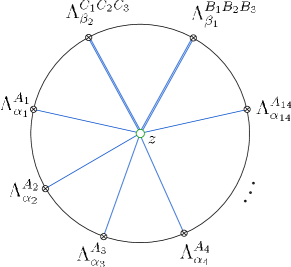
Figure 3: Contact and exchange contributions to a four-point amplitude in AdS${}_{5}\times S^{5}$

The resulting amplitude is

$$\frac{N_{c}^{1/2}}{g^{24}}\sum_{K>0}K^{\frac{25}{2}}\sum_{m|K}\frac{1}{m^{2}}\,{\rm e}^{2\pi iK\tau}\!\!\int\!\frac{{\rm d}^{4}z\,{\rm d}z_{0}}{z_{0}^{5}}\,{\rm d}^{5}\omega\,t_{16}\times$$

$$\times\prod_{i=1}^{14}{\mathcal{Y}}_{F}^{(0)}(\omega)\,K_{7/2}^{F}(z,z_{0};x_{i})\prod_{j=1}^{2}{\mathcal{Y}}_{F}^{(1)}(\omega)\,K_{9/2}^{F}(z,z_{0};y_{i})\,.$$ (452)

where ${\mathcal{Y}}_{F}^{(1)}(\omega)$ denotes the first excited fermionic spherical harmonic. The result (452) is again in agreement with the corresponding Yang–Mills calculation (400).

Non-minimal amplitudes of this type, involving KK excited states, are generalisations of the analogous minimal ones. Apart from the appearance of bulk-to-boundary propagators for fields of the appropriate mass, the only difference is in the five-sphere integrals, because of the presence of higher harmonics, which are necessary to reproduce the $\Omega$-dependence of the corresponding Yang–Mills expressions.

The study of the other class of non-minimal amplitudes is more complicated and yields some surprises. In order to describe the main features of these amplitudes we focus on the example of the process dual to the correlation function (385) involving sixteen fermionic operators, $\Lambda^{A}_{\alpha}$, in the $\mathbf{4}$ of SU(4) and four scalar operators, ${\mathcal{E}}^{AB}$, in the $\mathbf{10}$. As already observed, it is natural to expect that in these cases the amplitudes should involve couplings of order ${\alpha^{\prime}}^{5}$ and beyond. The operator ${\mathcal{E}}^{AB}$ in (386) is dual to a linear combination of the NS–NS and R–R two-forms with indices in the internal directions. The corresponding field strength, $G_{(3)}$, was defined in Sect. 18.1. Therefore a contact amplitude involving the vertex

$${\alpha^{\prime}}\int{\rm d}^{10}X\,\sqrt{-g}\,{\rm e}^{\phi/2}f_{2}^{(14,-14)}(\tau,\bar{\tau})\,G^{4}\,\lambda^{16}$$ (453)

represents an obvious candidate for the dual of the correlator (385). This process is represented in the second diagram of Fig. 4.

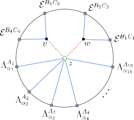
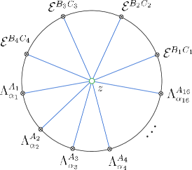
Figure 4: Contributions to the twenty-point amplitude dual to the correlation function (385).

This interpretation, however, leads to a puzzle. Using the dictionary (420) the twelve-derivative couplings at order ${\alpha^{\prime}}^{5}$ give rise to contributions of order $N_{c}^{-1/2}$, in fact

$$\frac{{\alpha^{\prime}}\,{\rm e}^{\phi/2}}{L}\sim N_{c}^{-1/2}\,,$$ (454)

which is not the behaviour expected from the Yang–Mills analysis. The leading contribution to the correlation function (385) is in fact of order $N_{c}^{1/2}$, as follows from (390)-(393).

The resolution of this mismatch requires the inclusion in the supergravity analysis of contributions of a type not encountered in the calculation of minimal amplitudes. These are exchange diagrams involving a D-instanton induced vertex as well as additional perturbative couplings. The relevant D-instanton vertices are those of order $1/{\alpha^{\prime}}$ in the expansion of the effective action, so that the resulting amplitudes give rise to contributions of order $N_{c}^{1/2}$, see (449). In order to generate contributions to non-minimal amplitudes one needs to include in the D-instanton vertices the fluctuations of the complex scalar, $\tau=\tau_{0}+\hat{\tau}$, as described at the end of Sect. 18.1.

In the case of the amplitude under consideration one needs to consider the vertex coupling sixteen dilatini with two additional insertions of $\hat{\tau}$ coming from the expansion of the exponential factor in the modular form $f^{(12,-12)}_{1}(\tau,\bar{\tau})$. The non-perturbative part of the effective vertex is

$$\frac{1}{{\alpha^{\prime}}}\int{\rm d}^{10}X\,\sqrt{-g}\,{\rm e}^{-25\phi/2}\,{\rm e}^{2\pi i\tau}\,\hat{\tau}^{2}\,t_{16}\,\lambda^{16}\,,$$ (455)

where only the $K=1$ contribution relevant for the comparison with the one-instanton sector in ${\mathcal{N}}=4$ SYM has been included. The amplitude contributing to the dual of the twenty-point correlator (385) is depicted on the l.h.s. of Fig. 4. The two bulk-to-bulk lines joining the D-instanton vertex at point $z$ to the points $v$ and $w$ are $\langle\hat{\tau}\hat{\bar{\tau}}\rangle$ propagators and the two cubic vertices are $\hat{\bar{\tau}}GG$ couplings from the classical type IIB action.

In evaluating this diagram, upon using dimensional reduction-like formulae as (443), one has to sum over all the contributions associated with the exchange of the KK excitations of the complex scalar. The coupling to the external three-forms restricts this sum to the states allowed by the $SO(6)$ selection rules enforced by the integration over the five sphere. In the present case there is only one allowed contribution, corresponding to the exchange of a complex scalar in the second KK excited level, i.e. a state in the representation $\mathbf{20^{\prime}}$ of $SO(6)\sim SU(4)$.

At first sight the resulting amplitude does not resemble the ${\mathcal{N}}=4$ SYM result: it is an exchange amplitude requiring integrations over three bulk points. However, because of the specific coupling involved the integrations over the positions of the two cubic couplings can be performed. This is because, after using expressions such as (443), one can integrate by parts the derivatives in each of the three-form field strengths onto the $\hat{\tau}$ scalar, and the cubic couplings schematically reduce to the form

$$(\partial^{2}+m_{\tau_{\mathbf{20^{\prime}}}})\hat{\tau}\,B_{ij}B^{ij}\,,$$ (456)

where $B$ is the complex combination of the NS–NS and R–R two-forms and the mass term comes from the derivatives in the $S^{5}$ directions. After the integration by parts one thus reconstructs the AdS₅ wave operator acting on the internal bulk-to-bulk propagators which then yield five-dimensional $\delta$-functions. The integrations at the points $v$ and $w$ in Fig. 4 can thus be computed and the exchange diagram reduces to a contact contribution. Therefore the net effect of the exchange diagram is to give rise to a new coupling in the AdS₅ effective action of the form

$$\frac{1}{g_{\rm s}^{2}{\alpha^{\prime}}}\int\frac{{\rm d}^{4}z\,{\rm d}z_{0}}{z_{0}^{5}}\,{\rm e}^{-25\phi/2}\,{\rm e}^{2\pi i\tau}\,t_{16}\,\lambda^{16}\,B^{4}\,,$$ (457)

where the factor of $g_{\rm s}^{-2}$ arises from the rescaling of the complex scalar, $\hat{\tau}$, needed to make its kinetic term canonically normalised.

The amplitude induced by this vertex (expressed in terms of SYM parameters) takes schematically the form

$$\frac{\sqrt{N_{c}}\,{\rm e}^{2\pi i\tau}}{g^{28}}\int\frac{{\rm d}^{4}z\,{\rm d}z_{0}}{z_{0}^{5}}\,\prod_{i=1}^{16}K_{7/2}^{F}(z,z_{0};x_{i})\prod_{j=1}^{4}K_{3}(z,z_{0};y_{j})\,,$$ (458)

which reproduces the leading large $N_{c}$ term in the ${\mathcal{N}}=4$ result (390) with the correct space-time dependence.

The amplitude involving the order ${\alpha^{\prime}}^{5}$ vertex $\lambda^{16}G^{4}$ in (453) gives rise to a contribution with the same space-time dependence, but of order $N_{c}^{-1/2}$. This sub-leading contribution is interpreted as corresponding to the $1/N_{c}$ correction in the SYM result (390).

The example of the above twenty-point function illustrates some features common to many non-minimal amplitudes. In general, unlike in the minimal cases, the amplitudes dual to non-minimal ${\mathcal{N}}=4$ correlation functions receive several contributions. Various effects such as those described in the previous example need to be taken into account to show agreement between the Yang–Mills and supergravity calculations. More details and other non-minimal examples are discussed in gk .

18.3 Beyond supergravity: the BMN limit

The AdS/CFT correspondence discussed in the previous sections is a very remarkable duality and the study of instanton effects has led to some of the most successful tests of its validity. In the formulation presented so far the duality has, however, some limitations. Because of our present limited understanding of the quantisation of string theory in non-trivial backgrounds such as AdS${}_{5}\times S^{5}$ the study of the gravity side of the correspondence is restricted to the supergravity approximation. Moreover, even in this regime, the strong–weak coupling nature of the duality makes the direct comparison of the two sides problematic. In this section we briefly review a very interesting limit of the correspondence, the so-called BMN limit bmn , which allows to overcome both the above limitations . The idea is to consider string theory in a background obtained from AdS${}_{5}\times S^{5}$ via a special procedure known as Penrose limit penlim . The result of the limit is a background with the geometry of a maximally supersymmetric gravitational plane-wave bfhp . Remarkably, despite the non-flatness of the metric and the presence of a R–R background, it is possible to quantise string theory in this geometry met ; mt . In bmn it has been proposed that strings propagating in this particular plane-wave background are dual to a certain sector of ${\mathcal{N}}=4$ SYM. The latter, usually referred to as the BMN sector, comprises operators of large scaling dimension, $\Delta$, and large charge, $J$, with respect to a $U(1)$ subgroup of the $SU(4)$ R-symmetry group. The possibility of quantising string theory in the plane-wave background has made the comparison between string and gauge theory possible beyond the supergravity approximation, albeit only in a specific sector of ${\mathcal{N}}=4$ SYM. Moreover, in this limit there exists a regime in which both sides of the correspondence are weakly coupled, so that the strong–weak coupling problem is also avoided.

At the heart of the correspondence proposed in bmn is a relation between the energy, $E$, of plane-wave string states and a combination of the scaling dimension and R-charge of the dual operators, which reads

$$\frac{1}{\mu}\,E=\Delta-J\,,$$ (459)

where the parameter $\mu$ is related to the value of the R–R self-dual five-form present in the background, see (464). The validity of (459) has been successfully tested in perturbation theory in a number of cases. Reviews of these results can be found in bmnrevs . In this subsection we present a brief overview of the non-perturbative tests carried out in gks1 ; gks2 ; gks3 .

In order to take the Penrose limit that gives rise to the plane-wave background we start with the AdS${}_{5}\times S^{5}$ metric written in global coordinates

$${\rm d}s^{2}=L^{2} \left[-\cosh^{2}\rho\,{\rm d}t^{2}+{\rm d}\rho^{2}+\sinh^{2}\rho\,{\rm d}\Omega_{3}^{2}+\right.$$

$$\left.\;+\cos^{2}\theta\,{\rm d}\psi^{2}+{\rm d}\theta^{2}+\sin^{2}\theta\,{\rm d}\tilde{\Omega}_{3}^{2}\right],$$ (460)

where $\Omega_{3}$ and $\tilde{\Omega}_{3}$ refer to angles parametrising two three-spheres inside AdS₅ and $S^{5}$ respectively. In this coordinate system one can choose

$$\tilde{x}^{\pm}=\pm\frac{1}{\sqrt{2}}(t\pm\psi)$$ (461)

as light-cone variables and define the new coordinates

$$x^{+}=\frac{1}{\mu}\tilde{x}^{+}\,,\qquad x^{-}=\mu L^{2}\tilde{x}^{-}\,,\qquad\rho=\frac{r}{L}\,,\qquad\theta=\frac{y}{L}\,,$$ (462)

where $\mu$ is an arbitrary scale. The Penrose limit is obtained sending $L$ to infinity while keeping $x^{\pm},\rho$ and $y$ “fixed”. The resulting metric is that of a plane-wave

$${\rm d}s^{2}=2{\rm d}x^{+}{\rm d}x^{-}-\mu^{2}x^{I}x^{I}({\rm d}x^{+})^{2}+{\rm d}x^{I}{\rm d}x^{I}\,,$$ (463)

where $x^{I}$, $I=1,\ldots,8$, are Cartesian coordinates such that $x^{I}x^{I}=r^{2}+y^{2}$. The original AdS${}_{5}\times S^{5}$ background has also a non-zero self-dual R–R five-form (419), which after the limit has non-vanishing components

$$F_{+1234}=F_{+5678}=2\mu\,,$$ (464)

with indices $1,2,\ldots,8$ corresponding to the $x^{I}$ directions .

The plane-wave background preserves the same (maximal) amount of supersymmetry as the original AdS${}_{5}\times S^{5}$. In fact at the level of the super-isometries the Penrose limit corresponds to an Inönü–Wigner contraction . The supergroup of isometries resulting from the contraction of $PSU(2,2|4)$ is $PSU(2|2)\times PSU(2|2)\times U(1)\times U(1)$ with maximal bosonic subgroup $H(4)^{2}\rtimes SO(4)\times SO(4)\times U(1)\times U(1)$, where $H(4)$ denotes the four-dimensional Heisenberg group bfhp . In the following we shall denote the two $SO(4)$ factors with $SO(4)_{C}$ and $SO(4)_{R}$, where the subscript refers to the fact that they are subgroups respectively of the conformal group and the R-symmetry group of the dual ${\mathcal{N}}=4$ SYM theory. The states in the string spectrum can therefore be labeled by quantum numbers characterising their transformation under $SO(4)_{C}\times SO(4)_{R}\times U(1)\times U(1)$. These are identified with two pairs of spins, $(s_{1},s_{2};s_{1}^{\prime},s_{2}^{\prime})$, and the light-cone energy and momentum, $(p_{+},p_{-})$, associated with translations in the $x^{+}$ and $x^{-}$ directions.

A very remarkable feature of the plane-wave background is that it allows the quantisation of string theory in the Green–Schwarz (GS) formalism  As shown in met , in the light-cone gauge the plane-wave GS string is described by a (massive) free world-sheet theory. This allows to carry out the quantisation essentially in same fashion as in flat space. The string action constructed in met is

$$S \!=\! \frac{1}{2\pi{\alpha^{\prime}}}\int_{-\infty}^{+\infty}{\rm d}\tau\int_{0}^{2\pi p_{-}}{\rm d}\sigma\,\left[\frac{1}{2}\partial_{+}X^{I}\partial_{-}X^{I}-\frac{1}{2}m^{2}X^{I}X^{I}+\right.$$ (465)

$$\left.\hskip 56.9055pt+i\left(S^{a}\partial_{+}S^{a}+\tilde{S}^{a}\partial_{-}\tilde{S}^{a}-2mS^{a}\Pi_{ab}\tilde{S}^{b}\right)\right],$$

where the mass parameter $m=\mu p_{-}{\alpha^{\prime}}$ has been introduced. In (465) the $X^{I}$’s denote the transverse coordinates of the string and the index $I=1,\ldots,8$ is in the ${\mathbf{8}_{\rm v}}$ of $SO(8)$. The $S^{a}$’s and $\tilde{S}^{a}$’s, $a=1,\ldots,8$, are GS fermions. These are $SO(8)$ spinors of the same chirality in the ${\mathbf{8}_{\rm s}}$. The matrix $\Pi$ is a product of $SO(8)$ $\gamma$-matrices, $\Pi=\gamma^{1}\gamma^{2}\gamma^{3}\gamma^{4}$. As usual in the light-cone gauge the non-physical components have been eliminated setting $X^{+}(\sigma,\tau)=2\pi{\alpha^{\prime}}p_{-}\tau$, whereas $X^{-}(\sigma,\tau)$ is expressed in terms of the $X^{I}$’s using the so-called Virasoro constraints which follow from consistency with the equation of motion for the world-sheet metric.

Since (465) describes a free theory the equations of motions lead to a standard mode expansion. For instance for the transverse bosons one finds

$$X^{I}(\sigma,\tau) \!=\! \cos(m\tau)\,x_{0}^{I}+\frac{1}{m}\sin(m\tau)\,p_{0}^{I}+$$ (466)

$$\!+\! i\sum_{n\neq 0}\frac{1}{\omega_{n}}\left({\rm e}^{-i\omega_{n}\tau+2i\pi n\sigma}\alpha^{I}_{n}+{\rm e}^{-i\omega_{n}\tau-2i\pi n\sigma}\tilde{\alpha}^{I}_{n}\right)\,,$$

where

$$\omega_{n}={\rm sign}(n)\sqrt{m^{2}+n^{2}}\,.$$ (467)

The GS fermions have a similar mode expansion with coefficients which will be denoted by $S^{a}_{\pm n}$ and $\tilde{S}^{a}_{\pm n}$.

Upon quantisation the coefficients in the expansion of the world-sheet fields give rise to creation and annihilation operators for the states in the string spectrum. In order to construct the physical creation and annihilation operators the $SO(8)$ oscillators need to be decomposed under $SO(4)_{C}\times SO(4)_{R}$. Massive excitations of the string are associated with non-zero oscillators. The bosonic ones, $\alpha^{I}_{n}$ and $\tilde{\alpha}^{I}_{n}$, are in the $\mathbf{8_{\rm v}}$ which decomposes as $\mathbf{8_{\rm v}}\to(\mathbf{4};\mathbf{1})\oplus(\mathbf{1};\mathbf{4})$, and one obtains

$$\alpha^{I}_{n}~{}\to~{}\alpha^{i}_{n}\,,~{}~{}\alpha^{\mu+5}_{n}\,,\qquad\tilde{\alpha}^{I}_{n}~{}\to~{}\tilde{\alpha}^{i}_{n}\,,~{}~{}\tilde{\alpha}^{\mu+5}_{n}\,,\qquad n\in\mathbbm{Z}\,,\quad n\neq 0\,,$$ (468)

where $i=1,2,3,4$ and $\mu=0,1,2,3$ are vector indices in $SO(4)_{R}$ and $SO(4)_{C}$ respectively. The fermions are in the $\mathbf{8_{\rm s}}$ which decomposes into $(\mathbf{2}_{L};\mathbf{2}_{L})\oplus(\mathbf{2}_{R};\mathbf{2}_{R})$. The fermionic oscillators are decomposed using the projectors $P_{\pm}=\frac{1}{2}(1\pm\Pi)$

$$S^{a}_{n}~{}\to~{}S^{\pm}_{n}=P_{\pm}S^{a}_{n}\,,\qquad\tilde{S}^{\pm}_{n}=P_{\pm}\tilde{S}^{a}_{n}\,,$$ (469)

which yield spinors with $SO(4)_{C}\times SO(4)_{R}$ chiralities $(+,+)$ and $(-,-)$.

The zero-modes in the expansion of the world-sheet fields are treated similarly. The bosonic ones, $x_{0}^{I}$ and $p_{0}^{I}$, associated with the transverse position and momentum of the string, are combined into

$$a^{I}=\frac{1}{\sqrt{2|m|}}(p_{0}^{I}-i|m|x_{0}^{I})\quad{\rm and}\quad{a^{I}}^{\dagger}=\frac{1}{\sqrt{2|m|}}(p_{0}^{I}+i|m|x_{0}^{I})\,.$$ (470)

These are then decomposed as in (468). The fermion zero-modes, $S_{0}$ and $\tilde{S}_{0}$, are combined into

$$\theta=\frac{1}{\sqrt{2}}(S_{0}+i\tilde{S}_{0})\quad{\rm and}\quad\bar{\theta}=\frac{1}{\sqrt{2}}(S_{0}-i\tilde{S}_{0})$$ (471)

and then further decomposed as

$$\theta_{L,R}=P_{+,-}\theta\,,\qquad\bar{\theta}_{L,R}=P_{+,-}\bar{\theta}\,.$$ (472)

The Fock space of states is built on a vacuum, $|0\rangle_{h}=|0,p_{-}\rangle_{h}$, defined as the state annihilated by $\theta_{R}$, $\bar{\theta}_{L}$, $a^{I}$ and all the non-zero oscillators of positive frequency. This is a non-degenerate bosonic state of zero mass usually referred to as the BMN vacuum. The fermionic zero-modes $\theta_{L}$ and $\bar{\theta}_{R}$ are creation operators and generate the supergravity multiplet acting on $|0\rangle_{h}$ mt . The bosonic zero-modes ${a^{I}}^{\dagger}$ create Kaluza–Klein-like excitations. The massive string modes are created by combinations of non-zero oscillators with negative frequencies, $\alpha^{i}_{-n}$, $\tilde{\alpha}^{i}_{-n}$, $\alpha^{\mu+5}_{-n}$, $\tilde{\alpha}^{\mu+5}_{-n}$, $S^{\pm}_{-n}$ and $\tilde{S}^{\pm}_{-n}$, acting on the BMN vacuum. Physical states, $|s\rangle_{\rm phys}$, are subject to the level matching condition

$$\left(N-\tilde{N}\right)|s\rangle_{\rm phys}=0\,,$$ (473)

where the left and right moving number operators are defined by

$$\begin{array}[]{l}\displaystyle N=\sum_{n=1}^{\infty}\left(\frac{n}{\omega_{n}}\,\alpha^{I}_{-n}\alpha^{I}_{n}+n\,S^{a}_{-n}S^{a}_{n}\right)\\ \displaystyle\tilde{N}=\sum_{n=1}^{\infty}\left(\frac{n}{\omega_{n}}\,\tilde{\alpha}^{I}_{-n}\tilde{\alpha}^{I}_{n}+n\,\tilde{S}^{a}_{-n}\tilde{S}^{a}_{n}\right)\,.\rule{0.0pt}{20.0pt}\end{array}$$ (474)

The string theory Hamiltonian can be expressed in terms of the above oscillators as

$$2p_{-}\,H \!=\! m\left({a^{I}}^{\dagger}a^{I}+\theta_{L}^{a}\bar{\theta}_{L}^{a}+\bar{\theta}_{R}^{a}\theta_{R}^{a}\right)+$$ (475)

$$\!+\! \sum_{k=1}^{\infty}\left[\alpha^{I}_{-k}\alpha_{k}^{I}+\tilde{\alpha}^{I}_{-k}\tilde{\alpha}_{k}^{I}+\omega_{k}\left(S^{a}_{-k}S^{a}_{k}+\tilde{S}^{a}_{-k}\tilde{S}^{a}_{k}\right)\right]\,.$$

From the form of the Hamiltonian (475) it is straightforward to compute the free string spectrum. The mass of a generic massive string excitation is

$$\frac{1}{\mu}\,M=\frac{1}{m}\sum_{n=1}^{\infty}\left(N+\tilde{N}\right)|\omega_{n}|\,,$$ (476)

with $\omega_{n}$ defined in (467) and $m=\mu p_{-}{\alpha^{\prime}}$.

In the following our discussion will focus on massive string states, which are more interesting in the context of the duality with ${\mathcal{N}}=4$ SYM since their masses receive quantum corrections. For simplicity we shall restrict our attention to states created by the $\alpha^{i}_{-n}$ and $\tilde{\alpha}^{i}_{-n}$ oscillators

$$|s\rangle=\alpha^{i_{1}}_{-n_{1}}\cdots\alpha^{i_{r}}_{-n_{r}}\cdots\tilde{\alpha}^{j_{1}}_{-m_{1}}\cdots\tilde{\alpha}^{j_{s}}_{-m_{s}}\cdots|0\rangle_{h}\,,$$ (477)

with $\sum_{r}n_{r}=\sum_{s}m_{s}$ to satisfy level-matching.

As has been mentioned before, the states in the spectrum are characterised by the their $SO(4)_{C}\times SO(4)_{R}$ quantum numbers, besides their mass and light-cone momentum. As in the original formulation of the AdS/CFT correspondence the quantum numbers associated with the symmetries on the two sides also dictate the map relating string states to composite operators in ${\mathcal{N}}=4$ SYM. Equation (462) leads to the following identifications

$$\begin{array}[]{l}\displaystyle\frac{1}{\mu}\,H\equiv\frac{1}{\mu}\,p_{+}=-i\partial_{+}=-i(\partial_{t}+\partial_{\psi})\to{\mathcal{D}}-{\mathcal{J}}\\ \displaystyle p_{-}=-i\partial_{-}=\frac{i}{2\mu L^{2}}(\partial_{t}-\partial_{\psi})\to\frac{1}{2\mu L^{2}}({\mathcal{D}}+{\mathcal{J}})\,,\end{array}$$ (478)

where, as usual, $L^{4}=4\pi g_{\rm s}N_{c}{\alpha^{\prime}}^{2}$. Equations (478) relate the string light-cone energy and momentum to linear combinations of the dilation operator, ${\mathcal{D}}$, and the generator, ${\mathcal{J}}$, of the $U(1)$ subgroup of the $SU(4)$ R-symmetry singled out in taking the Penrose limit. From the above relations it follows that in the $L\to\infty$ limit string states with finite energy and light-cone momentum correspond to SYM operators with values of ${\mathcal{D}}$ and ${\mathcal{J}}$ satisfying

$$\Delta\to\infty\,,\qquad J\to\infty\,,\qquad\Delta-J\quad{\rm finite}\,.$$ (479)

Operators with these properties form the BMN sector of ${\mathcal{N}}=4$ SYM. The explicit form of the operators dual to states in the plane-wave string spectrum was proposed in bmn . The starting point for the construction of such operators is the definition of the dual to the BMN vacuum which is identified with the operator

$${\mathcal{O}}=\frac{1}{\sqrt{JN_{c}^{J}}}\,{\rm Tr}\left(Z^{J}\right)\,,$$ (480)

where $Z$ is the complex combination of the ${\mathcal{N}}=4$ scalar fields with $J=1$ for which we choose $Z=2\varphi^{14}$ (see (337)-(338)). The operator (480) has $\Delta-J=0$ as expected for the dual of a zero energy state. Operators corresponding to the other states in the string spectrum are obtained inserting in the trace in (480) “impurities”, i.e. other elementary fields in the ${\mathcal{N}}=4$ fundamental multiplet. The action of each creation operator on the string side corresponds to the insertion of an impurity of a certain type . In particular the operators dual to states of the form (477) are

$${\mathcal{O}}^{i_{1}\ldots i_{k}}_{J;n_{1}\ldots n_{k}} \!=\! \frac{1}{\sqrt{J^{k-1}\left(\frac{g^{2}N_{c}}{8\pi^{2}}\right)^{J+k}}}\times$$ (483)

$$\!\times\! \begin{array}[t]{c}{\displaystyle\sum_{p_{1},\ldots,p_{k-1}=0}^{J}}\\ {\scriptstyle p_{1}+\cdots+p_{k-1}\leq J}\end{array}{\rm e}^{2\pi i[(n_{1}+\cdots+n_{k-1})p_{1}+(n_{2}+\cdots+n_{k-1})p_{2}+\cdots+n_{k-1}p_{k-1}]/J}\times$$

$$\!\times\! {\rm Tr}\left(Z^{J-(p_{1}+\cdots+p_{k-1})}\varphi^{i_{1}}Z^{p_{1}}\varphi^{i_{2}}\cdots Z^{p_{k-1}}\varphi^{i_{k}}\right)\,,$$ (484)

where the integers $n_{i}$ correspond to the mode numbers of the string state  and the action of the creation operators in (477) is in correspondence with the insertion of impurities, $\varphi^{i}$, for which we have the definitions

$$\begin{array}[]{ll}\displaystyle\displaystyle\varphi^{1}=\frac{1}{\sqrt{2}}\left(-\varphi^{13}+\varphi^{24}\right)\,,&\displaystyle\varphi^{2}=\frac{1}{\sqrt{2}}\left(\varphi^{12}+\varphi^{34}\right)\,,\\ \displaystyle\varphi^{3}=\frac{i}{\sqrt{2}}\left(-\varphi^{13}-\varphi^{24}\right)\,,&\displaystyle\varphi^{4}=\frac{i}{\sqrt{2}}\left(\varphi^{12}-\varphi^{34}\right)\,,\rule{0.0pt}{18.0pt}\end{array}$$ (485)

The four real scalars, $\varphi^{i}$, transform in the $(\mathbf{1};\mathbf{4})$ of $SO(4)_{C}\times SO(4)_{R}$ and the map between the operators (484) and the string states (477) is determined by the $SO(4)_{R}$ quantum numbers.

To make the comparison between string theory in the plane-wave background and the BMN sector of ${\mathcal{N}}=4$ SYM possible at a quantitative level one has to consider the large $N_{c}$ limit. The combination of the large $N_{c}$ limit with the limit of large $\Delta$ and $J$, implies that new effective parameters, $\lambda^{\prime}$ and $g_{2}$, arise bmn ; kpss ; mit1 , which are related to the ordinary ’t Hooft parameters, $\lambda$ and $1/N_{c}$, by a rescaling

$$\lambda^{\prime}=\frac{g^{2}N_{c}}{J^{2}}\,,\qquad g_{2}=\frac{J^{2}}{N_{c}}\,.$$ (486)

These in turn are related to the parameters of the plane-wave string theory by

$$m^{2}=(\mu p_{-}{\alpha^{\prime}})^{2}=\frac{1}{\lambda^{\prime}}\>,\qquad 4\pi g_{\rm s}m^{2}=g_{2}\,.$$ (487)

The double scaling limit defined by (479) and $N_{c}\to\infty$ with $J^{2}/N_{c}$ fixed connects the weak coupling regime of the gauge theory to string theory at small $g_{s}$ and large $m$. The property that in this limit physical quantities can be expanded in powers of the effective parameters, $\lambda^{\prime}$ and $g_{2}$, is referred to as BMN scaling.

Instanton effects in the BMN limit

Tests of the BMN limit of the AdS/CFT correspondence consist in verifying the validity of the relation

$$\frac{1}{\mu}\,H={\mathcal{D}}-{\mathcal{J}}\,.$$ (488)

This is an operator relation and it requires that the eigenvalues of the two sides be equal, i.e. masses of states in the plane-wave string spectrum, rescaled by a factor of $\mu$, should equal the combination $\Delta-J$ for the dual operators. In general the comparison requires the resolution of a mixing problem, i.e. the diagonalisation of the operators in (488).

The quantum corrections to the string mass spectrum are extracted from two-point amplitudes. At the perturbative level calculations of such amplitudes have been performed using string field theory methods. The non-perturbative corrections that we are interested in are induced by two-point amplitudes in which the external states are coupled to D-instantons. These quantum corrections to the string masses should be compared to instanton corrections to the eigenvalues of the operator ${\mathcal{D}}-{\mathcal{J}}$, i.e. to the anomalous dimensions of BMN operators since the charge $J$ is not renormalised.

The leading D-instanton contribution to a two-point amplitude is obtained coupling the external states to two disconnected disks, with Dirichlet boundary conditions, localised at the same space-time point. This is schematically depicted in Fig. 5.

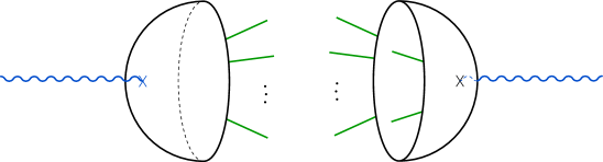
Figure 5: Leading D-instanton contribution to a two-point scattering amplitude.

The D-instanton in the plane-wave string theory can be described as a collective excitation of elementary closed string oscillators using the boundary state formalism gabgre . The construction of the D-instanton boundary state in the plane-wave background follows closely the approach used in gg2 for the light-cone GS string theory in flat space. The boundary state describing a D-instanton with transverse position $z^{I}$ will be denoted by $||z^{I}\rangle\!\rangle$. It is defined by the following gluing conditions

$$\begin{array}[]{l}\displaystyle\left(\alpha^{I}_{n}-\tilde{\alpha}^{I}_{-n}\right)||z^{I}\rangle\!\rangle=0\,,\\ \displaystyle\left(S^{a}_{n}+iM^{ab}_{n}\tilde{S}^{b}_{-n}\right)||z^{I}\rangle\!\rangle=0\rule{0.0pt}{17.0pt}\,,\qquad n\in\mathbbm{Z}\,,\end{array}$$ (489)

where the matrix $M_{n}$ is

$$M_{n}=\frac{1}{n}\left(\omega_{n}\mathbbm{1}-m\Pi\right)\,,$$ (490)

with $\omega_{n}$ given in (467). The explicit expression for $||z^{I}\rangle\!\rangle$ is gabgre

$$||z^{I}\rangle\!\rangle=(4\pi m)^{2}\exp\left(\sum_{k=1}^{\infty}\frac{1}{\omega_{k}}\alpha^{I}_{-k}\tilde{\alpha}^{I}_{-k}-iS^{a}_{-k}M_{k}\tilde{S}^{a}_{-k}\right)\,||z^{I}\rangle\!\rangle_{0}\,,$$ (491)

where $||z^{I}\rangle\!\rangle_{0}$ denotes the zero-mode part

$$||z^{I}\rangle\!\rangle_{0}={\rm e}^{-|m|(z^{I})^{2}/2}\,{\rm e}^{i\sqrt{2|m|}z^{I}{a^{I}}^{\dagger}}\,{\rm e}^{\frac{1}{2}{a^{I}}^{\dagger}{a^{I}}^{\dagger}}|0\rangle_{D}$$ (492)

and $|0\rangle_{D}=\theta^{1}_{L}\theta^{2}_{L}\theta^{3}_{L}\theta^{4}_{L}|0\rangle_{h}$.

The plane-wave background is maximally supersymmetric, i.e. it is invariant under 32 supersymmetries. These are divided into sixteen kinematical supersymmetries, which do not commute with the string Hamiltonian, and sixteen dynamical ones, which commute with the Hamiltonian. The boundary state (491)-(492) is annihilated by eight kinematical and eight dynamical supersymmetries as a consequence of the conditions (489). The other half of the supersymmetries acting on $||z^{I}\rangle\!\rangle$ generate the fermion zero-modes of the D-instanton. These are represented by the open strings attached to the boundary of the disks in Fig. 5. We shall denote the combinations of kinematical and dynamical supersymmetries which act non-trivially on the boundary state by $(\bar{q}_{L},\bar{q}_{R})$ and $Q^{-}$ respectively. The bosonic collective coordinates of the D-instanton correspond to its position in the ten-dimensional plane-wave geometry.

In order to compute a two-point amplitude of the type represented in Fig. 5 one needs to construct a state that includes the full dependence on the collective coordinates of the D-instanton and couples to two external states. We shall refer to such a state as a “dressed two-boundary state”. The latter describes the two disks in Fig. 5 and is obtained considering the product of two boundary states associated with distinct Fock spaces but located at the same position, $z^{I}$. The “dressing” corresponding to the inclusion of the dependence on the bosonic and fermionic collective coordinates is achieved acting with the bosonic and fermionic generators of the broken symmetries. Denoting the two Fock spaces with indices 1 and 2, the dressed two-boundary state can be written as

$$||V_{2};\bm{z},\eta,\epsilon\rangle\!\rangle={\rm e}^{iz^{+}(p_{1+}+p_{2+})}{\rm e}^{iz^{-}(p_{1-}+p_{2-})}\times$$ (493)

$$\times\left[\eta\left(Q^{-}_{1}+Q^{-}_{2}\right)\right]^{8}\left[\epsilon_{L}\left(q_{1L}+q_{2L}\right)\right]^{4}\left[\epsilon_{L}\left(q_{1L}+q_{2L}\right)\right]^{4}||z^{I}\rangle\!\rangle_{1}\otimes||z^{I}\rangle\!\rangle_{2}\,,$$

where $\bm{z}=(z^{I},z^{+},z^{-})$ is the ten-dimensional location of the D-instanton and the $SO(8)$ spinors $\eta$ and $\epsilon\!=\!(\epsilon_{L},\epsilon_{R})$ denote the fermionic collective coordinates associated with the dynamical and kinematical supersymmetries broken by the D-instanton.

The two-point amplitude that we are interested in is obtained coupling the dressed two-boundary state to a pair of external physical states and integrating over the bosonic and fermionic collective coordinates of the D-instanton. Denoting the incoming and outgoing states by $|s_{1}\rangle$ and $|s_{2}\rangle$, the one-particle irreducible part of the amplitude is

$${\mathcal{A}}=c\,g_{\rm s}^{7/2}\,{\rm e}^{2\pi i\tau}\int{\rm d}^{8}z\,{\rm d}z^{+}\,{\rm d}z^{-}\,{\rm d}^{8}\eta\,{\rm d}^{8}\epsilon\,(\langle s_{1}|\otimes\langle s_{2}|)||V_{2};\bm{z},\eta,\epsilon\rangle\!\rangle\,,$$ (494)

where $c$ is a numerical constant which has not been explicitly computed and the measure factor, $g_{\rm s}^{7/2}\,{\rm e}^{2\pi i\tau}$, follows from the comparison with the D-instanton induced contributions to the low energy effective action.

As an example of amplitude of the type (494) we consider the leading D-instanton contribution to the case in which $|s_{1}\rangle$ and $|s_{2}\rangle$ are particular states in the class (477). Specifically we consider $SO(4)_{R}$ singlet states with four impurities

$$\langle s_{1}|\otimes\langle s_{2}| \!=\! \frac{1}{\omega_{n_{1}}\omega_{n_{2}}\omega_{m_{1}}\omega_{m_{2}}}\,\varepsilon_{ijkl}\,\varepsilon_{i^{\prime}j^{\prime}k^{\prime}l^{\prime}}\times$$ (495)

$$\!\times\! {}_{h}\!\langle 0|\alpha^{(1)i}_{n_{1}}\alpha^{(1)j}_{n_{2}}\tilde{\alpha}^{(1)k}_{n_{1}}\tilde{\alpha}^{(1)l}_{n_{2}}\otimes{}_{h}\!\langle 0|\alpha^{(2)i^{\prime}}_{m_{1}}\alpha^{(2)j^{\prime}}_{m_{2}}\tilde{\alpha}^{(2)k^{\prime}}_{m_{1}}\tilde{\alpha}^{(2)l^{\prime}}_{m_{2}}\,,$$

where the prefactors ensure that the states are normalised to one. A generic four impurity state has three independent mode numbers, after imposing the level matching condition. In (495) we have made a special choice: each of the states contains two left- and two right-moving excitations with pairwise equal mode numbers. This is because only states of this type couple to a D-instanton at leading order in $g_{\rm s}$. This is a general property of D-instanton induced amplitudes: because of the way in which the creation operators enter in (491)-(492), the boundary state couples only to states with the same number of left- and two right-moving oscillators with pairwise matched mode numbers.

To proceed with the calculation of the leading D-instanton contribution we insert (495) into (494). The general strategy for the calculation of such amplitudes consists in expanding the $||z^{I}\rangle\!\rangle$ factors in the dressed boundary state in a power series retaining only the terms which do not annihilate the product $\langle s_{1}|\otimes\langle s_{2}|$ on the left. The integration over the collective coordinates $z^{+}$ and $z^{-}$ imposes conservation of light-cone energy and momentum. Because of the non-linear dispersion relation (467) energy conservation requires that the mode numbers in the incoming and outgoing states be equal. Of the remaining integrations those over the eight transverse $z^{I}$’s and over the eight $\epsilon$ fermionic moduli are trivial in the case of external states of the type we are considering . The non-trivial part of the calculation is the integration over the eight fermion moduli $\eta$

$$\langle s_{1}|\otimes\langle s_{2}|\int{\rm d}^{8}\eta\,\left[\eta(Q^{-}_{1}+Q^{-}_{2})\right]^{8}\exp\left[\sum_{n}\frac{1}{\omega_{n}}(\alpha^{(1)}_{-n}\tilde{\alpha}^{(1)}_{-n}+\right.$$ (496)

$$\hskip 28.45274pt\left.+\alpha^{(2)}_{-n}\tilde{\alpha}^{(2)}_{-n})-i(S^{(1)}_{-n}M_{n}\tilde{S}^{(1)}_{-n}+S^{(2)}_{-n}M_{n}\tilde{S}^{(2)}_{-n})\right]|0\rangle_{1}\otimes|0\rangle_{2}\,.$$

These integrations induce a coupling between the two disks, since the dynamical supercharges, $Q^{-}$, which couple to the $\eta$’s depend non-trivially on the non-zero string oscillators. The calculation is greatly simplified when one considers the large $m$ limit relevant for the comparison with ${\mathcal{N}}=4$ SYM at weak coupling. Since in this limit $M_{n}\sim m$, the dominant contribution to the amplitude with external states (495) is obtained retaining in the expansion of the boundary state two $SM\tilde{S}$ factors on each disk and distributing the eight $Q^{-}$’s evenly on the two disks. After some lengthy but straightforward algebra one obtains

$${\mathcal{A}}(n_{1},n_{2})=\varepsilon_{ijkl}\,\varepsilon_{i^{\prime}j^{\prime}k^{\prime}l^{\prime}}\>{\rm e}^{2\pi i\tau}\,g_{\rm s}^{7/2}\,m^{8}\,\frac{1}{n_{1}^{2}n_{2}^{2}}\,I^{ijkl,i^{\prime}j^{\prime}k^{\prime}l^{\prime}}_{\eta}$$ (497)

where

$$I^{ijkl,i^{\prime}j^{\prime}k^{\prime}l^{\prime}}_{\eta} \!=\! \int{\rm d}^{8}\eta\,\eta^{+}\gamma^{ij}\eta^{+}\eta^{+}\gamma^{kl}\eta^{+}\eta^{-}\gamma^{i^{\prime}j^{\prime}}\eta^{-}\eta^{-}\gamma^{k^{\prime}l^{\prime}}\eta^{-}=$$ (498)

$$\!=\! (\varepsilon^{ijkl}+\delta^{ik}\delta^{jl}-\delta^{il}\delta^{jk})(\varepsilon^{i^{\prime}j^{\prime}k^{\prime}l^{\prime}}-\delta^{i^{\prime}k^{\prime}}\delta^{j^{\prime}l^{\prime}}+\delta^{i^{\prime}l^{\prime}}\delta^{j^{\prime}k^{\prime}})\,.$$

In the case of the amplitude (497) the only contribution comes from the term containing the product of two $\varepsilon$-tensors in (498) and one gets

$${\mathcal{A}}(n_{1},n_{2})=576\>{\rm e}^{2\pi i\tau}\,g_{\rm s}^{7/2}\,m^{8}\,\frac{1}{n_{1}^{2}n_{2}^{2}}\,.$$ (499)

The same integral (498) arises in the calculation of two-point amplitudes between other $SO(4)_{C}\times SO(4)_{R}$ singlet four-impurity operators and in these cases the terms involving Kronecker $\delta$’s in $I^{ijkl,i^{\prime}j^{\prime}k^{\prime}l^{\prime}}_{\eta}$ can contribute.

The result (497) is the leading non-perturbative correction to the one particle irreducible part of the two-point amplitude and thus it yields the D-instanton correction to the mass matrix for states of the form (495)

$$\frac{1}{\mu}\,\delta M\sim\frac{{\rm e}^{2\pi i\tau}\,g_{\rm s}^{7/2}\,m^{7}}{(n_{1}n_{2})^{2}}=\frac{{\rm e}^{-\frac{8\pi^{2}}{g_{2}\lambda^{\prime}}+i\vartheta}g_{2}^{7/2}}{(n_{1}n_{2})^{2}}\,.$$ (500)

The SYM operators dual to the states in (495) are a special case of (484), i.e. four impurity $SO(4)_{C}\times SO(4)_{R}$ singlets. They are given by

$${\mathcal{O}}_{n_{1},n_{2},n_{3}} \!=\! \frac{\varepsilon_{ijkl}}{\sqrt{J^{3}(g^{2}N_{c})^{J+4}}}\begin{array}[t]{c}{\displaystyle\sum_{p,q,r=0}^{J}}\\ {\scriptstyle p+q+r\leq J}\end{array}{\rm e}^{2\pi i[(n_{1}+n_{2}+n_{3})p+(n_{2}+n_{3})q+n_{3}r]/J}\times$$ (503)

$$\!\times\! \,{\rm Tr}\left[Z^{J-(p+q+r)}\varphi^{i}Z^{p}\varphi^{j}Z^{q}\varphi^{k}Z^{r}\varphi^{l}\right]\,.$$ (504)

In order to compute the one instanton contribution to the matrix of anomalous dimensions for such operators one considers the two-point function

$$G(x_{1},x_{2})=\langle{\mathcal{O}}_{n_{1}n_{2}n_{3}}(x_{1})\,\bar{\mathcal{O}}_{m_{1}m_{2}m_{3}}(x_{2})\rangle\,.$$ (505)

The calculation proceeds as in the case of the correlators discussed in Sect. 15. In the semi-classical approximation one needs to compute the classical profiles of the operators ${\mathcal{O}}_{n_{1}n_{2}n_{3}}$ and $\bar{\mathcal{O}}_{m_{1}m_{2}m_{3}}$ and integrate them over the instanton moduli space. The profiles of the operator (504) and of its conjugate contain $2J+8$ fermion zero-modes each and thus (505) is non-minimal according to the terminology introduced in Sect. 15.

Although the calculation of the two-point function (505) presents no new conceptual difficulties, it involves rather complicated combinatorics associated with the distribution of the exact and non-exact fermion zero-modes in the two operators. Each of the two operators should soak up eight of the sixteen superconformal modes in the combination $(\zeta^{1})^{2}(\zeta^{2})^{2}(\zeta^{3})^{2}(\zeta^{4})^{2}$, while the remaining modes are of type $\nu^{A}$ and $\bar{\nu}^{A}$. Expanding the trace in (504) and in the conjugate operator one obtains a large number of terms satisfying this requirement. The double limit $N_{c}\to\infty$, $J\to\infty$, with $J^{2}/N_{c}$ fixed, simplifies somewhat the analysis. The dominant contributions in this limit come from certain specific distributions of the fermion modes. The large $N_{c}$ limit requires that all the $\bar{\nu}^{A}\nu^{B}$ bilinears be in the $\mathbf{6}$, see (396). Moreover at large $J$ the leading contributions to the operator profiles come from terms in which as many of the superconformal modes as possible are provided by the $Z$’s and $\bar{Z}$’s rather than by the impurities. This is because one gets roughly a multiplicity factor of $J$ associated with every $Z$ or $\bar{Z}$ providing one such mode. Taking into account these simplifications the calculation of the profiles of ${\mathcal{O}}_{n_{1}n_{2}n_{3}}$ and $\bar{\mathcal{O}}_{m_{1}m_{2}m_{3}}$, albeit rather tedious, is feasible. Eventually the dependence on the collective coordinates in all the relevant terms in the profile of the operator ${\mathcal{O}}_{n_{1}n_{2}n_{3}}$ reduces to

$$\frac{\rho^{8}}{[(x_{1}-x_{0})^{2}+\rho^{2}]^{J+8}}\left(\bar{\nu}^{[1}\nu^{4]}\right)^{J}\left[\left(\zeta^{1}\right)^{2}\left(\zeta^{2}\right)^{2}\left(\zeta^{3}\right)^{2}\left(\zeta^{4}\right)^{2}\right]\!(x_{1})\,.$$ (506)

Similarly all the terms in the classical profile of $\bar{\mathcal{O}}_{m_{1}m_{2}m_{3}}$ which contribute in the BMN limit contain the following factor

$$\frac{\rho^{8}}{[(x_{2}-x_{0})^{2}+\rho^{2}]^{J+8}}\left(\bar{\nu}^{[2}\nu^{3]}\right)^{J}\left[\left(\zeta^{1}\right)^{2}\left(\zeta^{2}\right)^{2}\left(\zeta^{3}\right)^{2}\left(\zeta^{4}\right)^{2}\right]\!(x_{2})\,.$$ (507)

After factoring out the dependence on the collective coordinates the dependence on the mode numbers, $n_{i}$ and $m_{i}$, is determined by sums of the form

$$K(n_{1},n_{2},n_{3};J) = \begin{array}[t]{c}{\displaystyle\sum_{p,q,r=0}^{J}}\\ {\scriptstyle p+q+r\leq J}\end{array}{\rm e}^{2\pi i[(n_{1}+n_{2}+n_{3})p+(n_{2}+n_{3})q+n_{3}r]/J}\times$$

$$\times\left[\frac{c_{1}}{4!}p(p-1)(p-2)(p-3)+\frac{c_{2}}{3!}qp(p-1)(p-2)+\cdots\right]\,,$$

where each term contains combinatorial factors and $c_{1},c_{2},\ldots$ are numerical coefficients.

The two-point function (505) is thus

$$\langle{\mathcal{O}}(x_{1})\,\bar{\mathcal{O}}(x_{2})\rangle_{\rm inst}=$$

$$=c(g,N_{c},J)\int\frac{{\rm d}^{4}x_{0}\,{\rm d}\rho}{\rho^{5}}\frac{\rho^{2J+16}}{[(x_{1}-x_{0})^{2}+\rho^{2}]^{J+8}[(x_{2}-x_{0})^{2}+\rho^{2}]^{J+8}}\times$$

$$\times\int{\rm d}^{8}\eta\,{\rm d}^{8}\bar{\xi}\,\prod_{A=1}^{4}\left[\zeta^{A}(x_{1})\right]^{2}\left[\zeta^{A}(x_{2})\right]^{2}\times$$

$$\times\int{\rm d}^{5}\Omega\,\left(\Omega^{14}\right)^{J}\left(\Omega^{23}\right)^{J}\,\left[K(n_{1},n_{2},n_{3};J)\,K(m_{1},m_{2},m_{3},J)\right]\,.$$ (511)

where $c(g,N_{c},J)$ contains the dependence on the parameters arising from the normalisation of the operators and the moduli space integration measure, as well as the factors of $g\sqrt{N_{c}}$ obtained rewriting the $(\bar{\nu}^{A}\nu^{B})_{\mathbf{6}}$ bilinears in terms of the angular variables $\Omega^{AB}$. In the large $J$ limit the sums in (18.3) can be approximated with integrals. For instance the first term becomes

$$\sum_{p,q,r=0}^{J}{\rm e}^{2\pi i[(n_{1}+n_{2}+n_{3})p+(n_{2}+n_{3})q+n_{3}r]/J}p(p-1)(p-2)(p-3)$$ (512)

$$\to J^{7}\int_{0}^{1}{\rm d}x\int_{0}^{1-x}{\rm d}y\int_{0}^{1-x-y}{\rm d}z\,{\rm e}^{2\pi i[(n_{1}+n_{2}+n_{3})x+(n_{2}+n_{3})y+n_{3}z]}\,x^{4}$$

From (511) and (512), recalling the analysis in Sect. 15, one can deduce the dependence of the two-point function on the parameters. There are numerous sources of powers of $g$, $N_{c}$ and $J$ in the calculation, but remarkably the final result can be expressed only in terms of the parameters $g_{2}$ and $\lambda^{\prime}$, as required by BMN scaling. In detail one gets

$$\underbrace{\left(\frac{1}{\sqrt{J^{3}(g^{2}N_{c})^{J+4}}}\right)^{2}}_{{\rm norm.~{}operators}}\times\underbrace{{\rm e}^{2\pi i\tau}g^{8}\sqrt{N_{c}}}_{{\rm measure}}\times\underbrace{\frac{\left(g\sqrt{N_{c}}\right)^{2J}}{J^{2}}}_{\begin{array}[]{c}\scriptstyle\nu,\bar{\nu}\\ \scriptstyle{\rm integrals}\end{array}}\times\underbrace{\frac{1}{J^{2}}}_{\begin{array}[]{c}\scriptstyle x_{0},\rho\\ \scriptstyle{\rm integrals}\end{array}}\times\underbrace{\left(J^{7}\right)^{2}}_{{\rm sums}}\sim$$ (517)

$$\sim\frac{J^{7}}{N_{c}^{7/2}}\,{\rm e}^{2\pi i\tau}=g_{2}^{7/2}\,{\rm e}^{-\frac{8\pi^{2}}{g_{2}\lambda^{\prime}}+i\vartheta}\,.$$ (518)

which is in agreement with the $\lambda^{\prime}$ and $g_{2}$ dependence of the string theory result (497).

The simple mode number dependence of the string two-point amplitude is more complicated to reproduce. In the SYM two-point function the dependence on the integers $n_{i}$ and $m_{i}$ is contained in the functions $K(n_{1},n_{2},n_{3};J)$ and $K(m_{1},m_{2},m_{3},J)$ defined in (18.3). Each term in these sums receives a large number of contributions resulting in very complicated expressions. However, combining all the contributions leads to impressive cancellations and a very simple result. In conclusion the one-instanton contribution to the two-point function (505) can be written in the form

$$G(x_{1},x_{2})=\frac{3^{2}\,(g_{2})^{7/2}\,{\rm e}^{-\frac{8\pi^{2}}{g_{2}\lambda^{\prime}}+i\vartheta}}{2^{41}\,\pi^{13/2}}\,\frac{1}{(n_{1}n_{2}m_{1}m_{2})}\frac{1}{(x_{12}^{2})^{J+4}}\log\left[\Lambda^{2}x_{12}^{2}\right]\,,$$ (519)

where $\Lambda$ is a scale that appears as a consequence of the logarithmic divergence in the $x_{0}$ and $\rho$ integrals, which signals a contribution to the matrix of anomalous dimensions. Notably the result is only non-zero if the mode numbers in the two operators are equal in pairs, again in agreement with string theory.

From the coefficient of (519) one can read off the contribution to the matrix of anomalous dimensions. The above calculation is not sufficient to determine the actual anomalous dimension of the operator (504) since this requires the diagonalisation of the matrix of two-point functions of all the operators with the same quantum numbers. However, all such two-point functions are expected to have the same dependence on $\lambda^{\prime}$ and $g_{2}$ found in (519). Therefore one can conclude that the behaviour of the leading instanton contribution to the anomalous dimension of four impurity $SO(4)_{C}\times SO(4)_{R}$ singlet operators is

$$\gamma_{\rm inst}\sim\frac{g_{2}^{7/2}\,{\rm e}^{-\frac{8\pi^{2}}{g_{2}\lambda^{\prime}}+i\vartheta}}{(n_{1}n_{2})^{2}}\,,$$ (520)

in agreement with (500). In view of the complexity of the calculation this result provides a striking test of the BMN proposal.

A number of other two-point string amplitudes and their dual correlation functions have been studied in gks1 ; gks2 ; gks3 . The many interesting results obtained in these papers can be summarised in the following statements.

• Four impurity operators in other representations of $SO(4)_{R}$ and the corresponding string states have two-point functions which behave as $(\lambda^{\prime})^{2}(g_{2})^{7/2}\exp(-8\pi^{2}/g_{2}\lambda^{\prime}+i\vartheta)$, i.e. they are suppressed by two powers of $\lambda^{\prime}$ with respect to those in the singlet sector.

• Two impurity operators have the same suppression. The calculation of instanton contributions to two-point functions of two impurity operators in ${\mathcal{N}}=4$ SYM is rather subtle because in order to saturate the integrations over the superconformal modes one needs to use the classical solution for the scalar fields involving six fermion modes, $\varphi^{(6)\,AB}$.

• Supergravity states and their KK excitations do not couple to the D-instanton boundary state and thus, as expected, their masses do not receive non-perturbative corrections. This result is far from obvious in the gauge theory and requires non-trivial cancellations which have not been explicitly verified.

• (D-)Instantons contribute to the mixing of states in the NS–NS and R–R sectors of the plane string theory .

• Instanton contributions to two-point functions of certain operators dual to R–R string states, i.e. operators with an even number of fermionic impurities, involve inverse powers of $\lambda^{\prime}$. Although this behaviour is rather surprising, it is not pathological in the $\lambda^{\prime}\to 0$ limit because the inverse powers of $\lambda^{\prime}$ are accompanied by the instanton weight $\exp(-8\pi^{2}/\lambda^{\prime}g_{2})$. These two-point functions vanish in perturbation theory.

It is notable that many of these results can be straightforwardly obtained in string theory where they are easily deduced from properties of the D-instanton boundary state, whereas they are much more complicated to obtain from a field theoretical calculation in ${\mathcal{N}}=4$ SYM.

19 Conclusions

We would like to conclude this long review by highlighting the many topics where Gabriele’s contributions along the years have been at the heart of the theoretical developments that have made our understanding of non-perturbative effects of field theory so deep and powerful.

Conceptually, perhaps the most important contributions in this direction have been his works on the foundation of the notion of effective action in a supersymmetric framework. The effective action for the ${\cal N}=1$ SYM theory VY and its extension to SQCD TVY are milestones along the way of dealing with the non-perturbative structure of field theory. These works appear as an immediate extension and generalisation of the approach established for the description of the low energy degrees of freedom of QCD WEIN ; GL , as soon as the fundamental rôle of anomalies was recognized WI ; RDWN ; DVNPV . The validation of the famous Witten-Veneziano formula WIVE for the $\eta^{\prime}$ mass, yielded by lattice simulations GIU , and the explicit instanton calculations, carried out in various instances in supersymmetric theories AKMRV , have beautifully confirmed the predictive power of the effective action approach both in a supersymmetric and in a non-supersymmetric context.

Together with many other important, independently derived, results ADSALL1 , these ideas have proved to be of enormous impact on the way we think today of possible extensions of the Standard Model.

We cannot end this review without mentioning what we consider the most important step of modern physics beyond field theory, namely the construction of the dual Veneziano amplitude veneziano , which is expressed by the remarkably simple formula

$$A(s,t)=\int_{0}^{1}{\rm d}x\,x^{-{\alpha^{\prime}}s-1}(1-x)^{-{\alpha^{\prime}}t-1}\,.$$ (521)

It is unanimously recognized that (521) represents the founding paper of String Theory. It took some time to realise that the infinite tower of “resonances” exchanged in the $s$ and $t$ channel are the excitations of an open bosonic string living in 26 dimensions. Planar duality, $A(s,t)=A(t,s)$, and the UV softness of the amplitude are exposed quite neatly by its geometric interpretation in terms of vertex operators inserted on the boundary of a disk. The presence of a massless vector excitation has brought String Theory to be the most credited candidate for the unification of all interactions, including gravity. In this respect, the graviton comes in as the massless excitation of the closed string spectrum and its vertex operator is a sort of “square” of the vertex operator for the massless vector of the Veneziano amplitude. That open strings might be considered more fundamental than closed strings is something which seems to emerge in all modern approaches, where D-branes and their open string excitations are used to describe interactions mediated by gauge bosons. We want also to recall that in a somewhat more distant context string excitations have been shown to be able to account for the microscopic degrees of freedom of Black Holes, thus yielding what is considered today the only satisfactory solution to the holographic puzzle of Black Hole thermodynamics VAST .

In the present review we have briefly sketched the enormous simplification that open strings bring into the ADHM construction of instantons. However, for lack of space we had no chance to stress the far-reaching consequences of ideas underlying the Veneziano amplitude in the quest for unification and in the process of clarification of the many puzzles of quantum gravity. We dare to conclude by saying that we expect the Veneziano amplitude to be among the basic blocks of any consistent formulation of the fundamental laws of Nature.

Acknowledgments

Discussions with Massimo Testa, Yassen Stanev and especially Michael Green are gratefully acknowledged. The work of SK was supported in part by a Marie Curie Intra-European Fellowship and by the EU-RTN network Constituents, Fundamental Forces and Symmetries of the Universe (MRTN-CT-2004-005104).

20 – Notations

$\bullet$ Generalities

We work in Euclidean metric with $g^{E}_{\mu\nu}=\delta_{\mu\nu}$. Factors of the gauge coupling constant, $g$, will be explicit everywhere. We are interested in computing expectation values of gauge invariant (possibly multi-local) renormalisable, composite operators, i.e. functional integrals of the type

$$\langle O\rangle\!=\!\frac{1}{Z}\!\int\!{\cal D}\mu(\psi,\bar{\psi}){\cal D}A_{\mu}\exp\big{[}\!-S_{\rm YM}+\!\int\!{\rm d}^{4}x\,\bar{\psi}({\mbox{$\not\!\!D$}}+m)\psi\big{]}O[\psi,\bar{\psi},A_{\mu}]\,,$$ (522)

where $\not\!\!D$ can be either a Dirac or a Weyl–Dirac operator (see below) and $Z$ is a similar functional integral with $O$ replaced by the identity operator.

$\bullet$ Yang–Mills action

The pure Yang–Mills action has the form

$$S_{\rm YM}=\frac{1}{2}\int{\rm d}^{4}x\,{\rm Tr}[F_{\mu\nu}F_{\mu\nu}]=\frac{1}{4}\int{\rm d}^{4}x\sum_{a}F^{a}_{\mu\nu}F^{a}_{\mu\nu}\,,$$ (523)

$$F_{\mu\nu}=T^{a}F^{a}_{\mu\nu}\,,\qquad F_{\mu\nu}=\partial_{\mu}A_{\nu}-\partial_{\nu}A_{\mu}+ig[A_{\mu},A_{\nu}]\,.$$ (524)

$\bullet$ Some group theory formulae

In (523) the matrices $T^{a}\equiv T^{a}_{{\bf N_{c}}}$, $a=1,2,\ldots,N^{2}_{c}-1$ are the $SU(N_{c})$ generators in the fundamental representation, ${\bf N_{c}}$. In general the generators, $T_{{\bf R}}$, in the (irreducible) representation ${\bf R}$ are normalised according to the formula

$${\rm Tr}\big{[}T_{{\bf R}}^{a}T^{b}_{{\bf R}}\big{]}=\ell[{\bf R}]\delta^{ab}\,,$$ (525)

with $\ell[{\bf R}]$ the Dynkin index of the representation. It is customary to normalise generators in the ${\bf N_{c}}$, ${\bf\bar{N}_{c}}$ and ${\bf Adj}$ representations so that

$$\ell[{\bf N_{c}}]=\ell[{\bf\bar{N_{c}}}]=\frac{1}{2}\,,\qquad\ell[{\bf Adj}]=N_{c}\,.$$ (526)

Taking the trace of the equation which defines the quadratic Casimir operator of the representation ${\bf R}$

$$\sum_{a}T_{{\bf R}}^{a}T^{a}_{{\bf R}}=c_{2}[{\bf R}]\mathbbm{1}_{{\rm dim}({\bf R})\times{\rm dim}({\bf R})}\,,$$ (527)

and using (525), one gets the useful relation

$$c_{2}[{\bf R}]{\rm dim}({\bf R})=\ell[{\bf R}]{\rm dim}(G)\,.$$ (528)

$\bullet$ Dirac fermions

The Euclidean action of a Dirac fermion, $\psi$, $\bar{\psi}$, in the representation ${\bf R}$ of the gauge group $SU(N_{c})$ takes the form

$$S_{\rm DF}=\int{\rm d}^{4}x\,\bar{\psi}_{r}D^{r}_{\mu s}[{\bf R}]\gamma_{\mu}\psi^{s}\,,\quad r,s=1,\ldots,{\rm dim}({\bf R})\,,$$ (529)

where Dirac indices are understood and

$$D^{r}_{\mu s}[{\bf R}]=\partial_{\mu}\delta^{r}_{s}-g(T^{a}_{{\bf R}})^{r}_{s}A_{\mu}^{a}\,.$$ (530)

In (529) hermitean $\gamma$-matrices are used, satisfying the anti-commutation relations $\{\gamma_{\mu},\gamma_{\nu}\}=2\delta_{\mu\nu}$.

$\bullet$ Weyl fermions

The Euclidean action of a Weyl fermion, $\lambda^{a}_{\alpha},\bar{\lambda}^{a}_{\dot{\alpha}}$ ($\alpha,\dot{\alpha}=1,2$) belonging to the adjoint representation of the gauge group $SU(N_{c})$ takes the form

$$S_{\rm WF}=\int{\rm d}^{4}x\,\bar{\lambda}^{a}_{\dot{\alpha}}D^{ab}_{\mu}[{\bf Adj}]\bar{\sigma}_{\mu}^{\dot{\alpha}\alpha}\lambda^{b}_{\alpha}\,,$$ (531)

where

$$D_{\mu}^{ab}[{\bf Adj}]=\partial_{\mu}\delta^{ab}-gf^{abc}A_{\mu}^{c}\,,$$ (532)

$$\bar{\sigma}_{\mu}=(\mathbbm{1},-i\sigma_{k})\,,$$ (533)

with $\sigma_{k}$ the Pauli matrices. It is also useful to introduce the matrices $(\sigma_{\mu})_{\alpha\dot{\alpha}}$

$$\sigma_{\mu}=(\mathbbm{1},i\sigma_{k})\,.$$ (534)

and the definitions

$$(\sigma_{\mu\nu})_{\alpha}^{\beta}=\frac{1}{2}(\sigma_{\mu\alpha\dot{\alpha}}\bar{\sigma}_{\nu}^{\dot{\alpha}\beta}-\sigma_{\nu\alpha\dot{\alpha}}\bar{\sigma}_{\mu}^{\dot{\alpha}\beta})\,,$$ (535)

$$(\bar{\sigma}_{\mu\nu})_{\dot{\alpha}}^{\dot{\beta}}=\frac{1}{2}(\bar{\sigma}_{\mu}^{\dot{\beta}\alpha}\sigma_{\nu\alpha\dot{\alpha}}-\bar{\sigma}_{\nu}^{\dot{\beta}\alpha}\sigma_{\mu\alpha\dot{\alpha}})\,.$$ (536)

$\bullet$ The SYM action

The Euclidean action of the minimal ${\cal N}=1$ supersymmetric gauge theory (Super Yang–Mills, SYM), $S_{\rm SYM}$, when written in components, is simply given by the sum of (523) and (531). The classical action is invariant under the $U_{\lambda}(1)$ R-symmetry RSYM

$$\lambda\to{\rm e}^{i\alpha}\lambda\,,\qquad A_{\mu}\,\,{\rm untouched}\,.$$ (537)

Quantum mechanically this symmetry is anomalous with

$$\partial_{\mu}J^{(\lambda)}_{\mu}=2i\ell[{\bf Adj}]\frac{g^{2}}{32\pi^{2}}F_{\mu\nu}^{a}\tilde{F}_{\mu\nu}^{a}=2iN_{c}\frac{g^{2}}{32\pi^{2}}F_{\mu\nu}^{a}\tilde{F}_{\mu\nu}^{a}\,,$$ (538)

$$J^{(\lambda)}_{\mu}=\bar{\lambda}_{\dot{\alpha}}^{a}\bar{\sigma}_{\mu}^{\dot{\alpha}\alpha}\lambda_{\alpha}^{a}\,,$$ (539)

but has a non-anomalous discrete subgroup

$$\mathbbm{Z}_{2N_{c}}=\{z_{k}={\rm e}^{i\alpha_{k}}\,,\alpha_{k}=2\pi k/2N_{c}\,,k=1,2,\ldots,2N_{c}\}\,.$$ (540)

This important statement can be proved in different ways. An elegant proof makes use of the (natural) extension of SYM in which a $\vartheta$ term is added to the action (see last section of Appendix C). In this situation under a $U_{\lambda}(1)$ rotation of the gluino fields in the functional integral, we get the (anomalous) WTI

$$\langle O_{1}(x_{1})\ldots O_{n}(x_{n})\rangle^{(\vartheta)}=\langle O_{1}(x_{1})\ldots O_{n}(x_{n})\rangle^{(\vartheta+2N_{c}\alpha)}\,.$$ (541)

Since the theory is classically invariant under such a rotation (the transformation $u(\alpha)O_{k}u^{\dagger}(\alpha)=\exp{(i\eta_{k}\alpha)}O_{k}$, with $\eta_{k}$ the $U_{\lambda}(1)$ charge of $O_{k}$ leaves invariant the correlator if the vacuum is annihilated by the unitary operator $u(\alpha)$), the only effect of the transformation is to change the value of the $\vartheta$ angle. The change does not affect physics if

$$2N_{c}\alpha=2n\pi\,,\quad n\in\mathbbm{Z}\,.$$ (542)

Clearly this result holds for any value of $\vartheta$, thus also at $\vartheta=0$.

When written in superfields, the SYM action takes the form RSYM

$$S_{\rm SYM}=\int{\rm d}^{4}x\,{\rm d}^{2}\theta\,{\rm Tr}[W_{\alpha}W^{\alpha}]\,,$$ (543)

$$W_{\alpha}=-\frac{1}{4}\bar{D}^{2}\big{(}{\rm e}^{-gV}D_{\alpha}{\rm e}^{gV}\big{)}\,,$$ (544)

$$V(x,\theta)=C(x)+\theta\mu(x)+\bar{\theta}\bar{\mu}(x)+{1\over 2}\theta^{2}S(x)+{1\over 2}\bar{\theta}^{2}\bar{S}(x)+$$

$$+\,\theta\sigma^{\mu}\bar{\theta}A_{\mu}(x)+{1\over 2}\bar{\theta}^{2}\theta\lambda(x)+{1\over 2}\theta^{2}\bar{\theta}\bar{\lambda}(x)+{1\over 4}\theta^{2}\bar{\theta}^{2}D(x)+\ldots\,,$$ (545)

where dots stand for terms that can be expressed as derivatives of the fields already present in (545).

$\bullet$ The SQCD action

The Euclidean action of the ${\cal N}=1$ supersymmetric theory which more closely resembles QCD is obtained by coupling in a supersymmetric and gauge invariant way to the SYM supermultiplet $N_{f}$ pairs of matter chiral superfields fields ($f=1,\ldots,N_{f}$, $r=1,\ldots,N_{c}$)

$$\Phi_{f}^{r}(x)=\phi_{f}^{r}(y)+\sqrt{2}\theta^{\alpha}\psi^{r}_{\alpha f}(y)+\theta^{2}F_{f}^{r}(y)\,,\qquad y_{\mu}=x_{\mu}+i\theta\sigma_{\mu}\bar{\theta}\,,$$ (546)

$$\tilde{\Phi}_{r}^{f}(x)=\tilde{\phi}_{r}^{f}(y)+\sqrt{2}\theta^{\alpha}\tilde{\psi}_{\alpha r}^{f}(y)+\theta^{2}\tilde{F}_{r}^{f}(y)\,,$$ (547)

belonging to the representations ${\bf N_{c}}$ and ${\bf\bar{N}_{c}}$, respectively, of the gauge group. In this way the gauge invariant mass term

$$S_{\rm SQCD}^{\rm mass}=\sum_{f}\Big{[}m_{f}\int{\rm d}^{4}x\sum_{\alpha r}\tilde{\psi}^{\alpha f}_{r}\psi_{\alpha f}^{r}+m^{*}_{f}\int{\rm d}^{4}x\sum_{\dot{\alpha}r}\bar{\psi}_{\dot{\alpha}r}^{f}{\bar{\tilde{\psi}}}^{\dot{\alpha}r}_{f}+$$

$$+|m_{f}|^{2}\int{\rm d}^{4}x\sum_{r}(\phi^{*f}_{r}\phi^{r}_{f}+\tilde{\phi}^{f}_{r}\tilde{\phi}^{*r}_{f})\Big{]}$$ (548)

can be constructed. The rest of the action is completely standard and can be found in any textbook or, for instance, in AKMRV .

$\bullet$ The “flavour” symmetries of the SQCD action

I) The classical SQCD action is invariant under the $U_{\lambda}(1)$ R-symmetry RSYM   which now transforms in a non-trivial way gluinos and scalars according to

$$\lambda\to{\rm e}^{i\alpha}\lambda\,,\quad\phi\to{\rm e}^{i\alpha}\phi\,,\quad\tilde{\phi}\to{\rm e}^{i\alpha}\tilde{\phi}\,,\quad+\quad{\rm complex\,\,conjugate\,,}$$

$$A_{\mu}\,,\quad\psi,\bar{\psi}\,,\quad\tilde{\psi},\bar{\tilde{\psi}}\,,\quad{\rm untouched}\,.$$ (549)

The $U_{\lambda}(1)$ R-symmetry of SQCD is anomalous with the same anomaly as in SYM (see (538)). Again only the $\mathbbm{Z}_{2N_{c}}$ subgroup is unbroken. With respect to the SYM case $J^{(\lambda)}_{\mu}$ must now be augmented with the inclusion of the matter contribution and reads

$$J^{(\lambda)}_{\mu}=\bar{\lambda}_{\dot{\alpha}}^{a}\bar{\sigma}_{\mu}^{\dot{\alpha}\alpha}\lambda_{\alpha}^{a}+\sum_{f}\Big{\{}\big{[}i\phi^{f*}\!\buildrel\leftrightarrow\over{\partial}_{\mu}\!\phi_{f}\big{]}+\big{[}\phi_{f}\to\tilde{\phi}^{f}\big{]}\Big{\}}\,.$$ (550)

II) The massless theory with $N_{f}$ flavours possesses a global $SU(N_{f})\times SU(N_{f})\times U_{V}(1)\times U_{A}(1)$ symmetry. The chiral $SU(N_{f})\times SU(N_{f})$ symmetry is broken by matter mass terms. For instance, if all masses are equal ($m_{f}=m$), the unbroken subgroup is the diagonal vector group $U_{V}(N_{f})$, while, if all masses are different ($m_{1}\neq m_{2}\neq\ldots\neq m_{f}$), the leftover unbroken subgroup is $U(1)^{N_{f}}$.

III) The $U_{A}(1)$ transformation

$$(\phi,\psi)\to{\rm e}^{i\alpha}(\phi,\psi)\,,\quad(\tilde{\phi},\tilde{\psi})\to{\rm e}^{i\alpha}(\tilde{\phi},\tilde{\psi})\,,\quad+\quad{\rm complex\,\,conjugate\,,}$$

$$\lambda\,,\quad A_{\mu}\,,\quad{\rm untouched}\,.$$ (551)

is classically a symmetry at vanishing masses, but it is quantum-mechanically anomalous with

$$\partial_{\mu}J^{(A)}_{\mu}=2iN_{f}\frac{g^{2}}{32\pi^{2}}F_{\mu\nu}^{a}\tilde{F}_{\mu\nu}^{a}\,,$$ (552)

$$J^{(A)}_{\mu}=\sum_{f}\Big{\{}\big{[}\bar{\psi}_{\dot{\alpha}}^{f}\bar{\sigma}_{\mu}^{\dot{\alpha}\alpha}\psi_{\alpha f}+i\phi^{*f}\!\buildrel\leftrightarrow\over{\partial}_{\mu}\!\phi_{f}\big{]}+\big{[}(\phi_{f},\psi_{f})\to(\tilde{\phi}^{f},\tilde{\psi}^{f})\big{]}\Big{\}}\,.$$ (553)

IV) Often, instead of $U_{\lambda}(1)$, the linear combination

$$U_{R}(1)=\frac{3}{2}U_{\lambda}(1)-\frac{1}{2}U_{A}(1)$$ (554)

is introduced because the associated current belongs to the current supermultiplet FZPS . This classical symmetry is anomalous and from (538) and (552) we see that the associated current obeys the anomaly equation

$$\partial_{\mu}{J}_{\mu}^{(R)}=i(3N_{c}-N_{f})\frac{g^{2}}{32\pi^{2}}F_{\mu\nu}^{a}\tilde{F}_{\mu\nu}^{a}\,.$$ (555)

V) It is possible to construct a non-anomalous, exactly conserved current, ${J}_{\mu}^{({\hat{A}})}$, out of the two anomalous currents $J^{(A)}_{\mu}$ and $J^{(\lambda)}_{\mu}$ (see (553) and (550)). One finds

$${J}_{\mu}^{({\hat{A}})}=-N_{f}J^{(\lambda)}_{\mu}+N_{c}J^{(A)}_{\mu}\,.$$ (556)

The transformations induced on the fields by the associated $U_{\hat{A}}(1)$ symmetry (556) are

$$(\phi,\tilde{\phi})\to{\rm e}^{i(N_{c}-N_{f})\alpha}(\phi,\tilde{\phi})\,,\,\,\,(\psi,\tilde{\psi})\to{\rm e}^{iN_{c}\alpha}(\psi,\tilde{\psi})\,,\,\,\,+\,\,\,\,{\rm complex\,\,conjugate}\,,$$

$$\lambda\to{\rm e}^{-iN_{c}\alpha}\lambda\,,\quad+\quad{\rm complex\,\,conjugate}\,.$$ (557)

VI) In the Table below we recollect for convenience the charges of elementary and composite gauge and matter fields under the various $U(1)$’s we have introduced. In the last two rows we report the coefficient of the anomaly of the associated current in units of $Q=\frac{g^{2}}{32\pi^{2}}F_{\mu\nu}^{a}\tilde{F}_{\mu\nu}^{a}$ and we indicate whether the conservation of the current is broken by mass terms or not.

Field	$SU(N_{f})$	$SU(N_{f})$	$U_{A}(1)$	$U_{R}(1)$	$U_{\hat{A}}(1)$	$U_{\lambda}(1)\!=\!U_{A}^{PQ}(1)$	$U_{V}(1)$
$\lambda$	${\bf 1}$	${\bf 1}$	0	3/2	-$N_{f}$	1	0
$\psi$	${\bf N_{f}}$	${\bf 1}$	1	1	$N_{c}$	0	1
$\phi$	${\bf N_{f}}$	${\bf 1}$	1	-1/2	$N_{c}-N_{f}$	1	0
$\tilde{\psi}$	${\bf 1}$	${\bf N_{f}}$	1	1	$N_{c}$	0	-1
$\tilde{\phi}$	${\bf 1}$	${\bf N_{f}}$	1	-1/2	$N_{c}-N_{f}$	1	0
$S|_{\theta=0}$	${\bf 1}$	${\bf 1}$	0	3	$-2N_{f}$	2	0
$T^{f}_{h}|_{\theta=0}$	${\bf N_{f}}$	${\bf N_{f}}$	2	2	$2(N_{c}-N_{f})$	2	0
Anomaly	/	/	$2N_{f}$	$3N_{c}-N_{f}$	0	$2N_{c}$	0
Mass term	Yes	Yes	Yes	Yes	Yes	No	No

Table 1: The $SU(N_{f})\times SU(N_{f})$ quantum numbers and $U(1)$-charges of elementary and composite fields of SQCD. The anomaly associated with each $U(1)$ current is given in units of ${g^{2}}/{32\pi^{2}}F^{a}_{\mu\nu}\tilde{F}^{a}_{\mu\nu}$. In the last line by “Yes” (“No”) we mean that the corresponding symmetry is (is not) broken by the presence of mass terms.

$\bullet$ Gluino zero modes

The explicit expression of the $2N_{c}$ gluino zero modes endowed with the correct normalisation $\int{\rm d}^{4}x\,\sum_{a}\lambda^{a\alpha}(x)\lambda^{a*}_{\alpha}(x)=1$ is (the index counting the $2N_{c}$ zero modes is indicated in parenthesis)

$$(\lambda^{\alpha}_{(k)})^{s}_{r}(x)=\frac{1}{\pi}(\delta^{\alpha}_{r}\delta^{s}_{k}-\epsilon^{\alpha s}\epsilon_{rk})\rho^{2}(f(x))^{2}\,,\quad k=1,2\,,$$ (558)

$$(\lambda^{\alpha(\dot{\alpha})})^{s}_{r}(x)=-\frac{i}{\sqrt{2}\pi}\bar{\sigma}^{\dot{\alpha}\beta}_{\mu}(x-x_{0})_{\mu}(\delta^{\alpha}_{r}\delta^{s}_{\beta}-\epsilon^{\alpha s}\epsilon_{r\beta})\rho(f(x))^{2}\,,\quad\dot{\alpha}=1,2\,,$$ (559)

$$(\lambda^{\alpha}_{(\pm i)})^{s}_{r}(x)=\frac{1}{\sqrt{2}\pi}(\delta^{\alpha}_{r}\delta^{s}_{i}\pm\epsilon^{\alpha s}\delta_{ri})\rho(f(x))^{3/2}\,,\quad i=1,\ldots,N_{c}-2\,,$$ (560)

with

$$f(x)=\frac{1}{(x-x_{0})^{2}+\rho^{2}}\,.$$ (561)

The first four modes are $SU(2)$ triplets, while the last $2(N_{c}-2)$ are doublets. The four triplets can be directly generated from the expression (24) by acting on it with anyone of two supersymmetric and two superconformal transformations that are unbroken in the background instanton field. They are often called “exact zero modes” in the literature, see for instance KHETAL and references therein. This name originates from the following observation. Effectively the overall field configuration which is relevant for the kind of computations we have presented in Sect. 4 (see Sect. 14 for further applications) is given by the gauge instanton solution, the associated set of fermionic zero modes and the expression of the scalar fields that are obtained by solving their linearised classical e.o.m., i.e. the e.o.m. that result upon neglecting the quartic scalar self-interaction terms. The reason for neglecting such terms is that the latter would give rise to contributions of higher order in $g$ compared to the leading ones we have been keeping. When the action of the theory is computed in this approximation and on the above field configuration, it just happens that the result does not depend on the fermionic collective coordinates associated with the four $SU(2)$ triplet zero modes of (558) and (559). The other fermionic zero modes will give origin to quartic terms in the remaining $2(N_{c}-2)$ fermionic collective coordinates (see Sect. 14).

21 – Bosonic collective coordinates and functional integration

In this Appendix we want to explain how one can compute the pure gauge part of the functional integration in the semi-classical approximation around a non-trivial instantonic background. We will follow the method of YAF , which neatly explains how to deal with the problem of bosonic zero modes and the consequent need of introducing collective coordinates.

In the semi-classical approximation one starts by expanding the (gauge) action around the (instanton) classical solution, keeping only terms up to quadratic fluctuations. Setting

$$A_{\mu}=A^{I}_{\mu}+Q_{\mu}\,,$$ (562)

one gets in this way

$$S_{\rm YM}=S^{I}-\frac{1}{2}\int{\rm d}^{4}x\,{\rm Tr}\big{[}Q_{\mu}{\cal M}_{\mu\nu}(A^{I})Q_{\nu}\big{]}+{\mbox{O}}(Q^{3})\,,$$ (563)

where

$$S^{I}=\frac{8\pi^{2}}{g^{2}}|K|\,,$$ (564)

$${\cal M}_{\mu\nu}(A^{I})=-D^{2}(A^{I})\delta_{\mu\nu}+D_{\mu}(A^{I})D_{\nu}(A^{I})-2[F_{\mu\nu}^{I},\cdot\,]\,,$$ (565)

$$D_{\mu}(A^{I})=\partial_{\mu}+g[A^{I}_{\mu},\cdot\,]\,.$$ (566)

The operator ${\cal M}_{\mu\nu}(A^{I})$ has quite a large manifold of (normalisable and non-normalisable) zero modes. Not only it is annihilated by all the functions of the form $D_{\nu}(A^{I})F(x)$, as a consequence of gauge invariance, but also by the $4|K|N_{c}$ normalisable vectors that are obtained by differentiating the instanton field configuration with respect to the $4|K|N_{c}$ parameters, $\beta_{i}$, $i=1,\ldots,4|K|N_{c}$ (bosonic collective coordinates in the following), upon which the most general classical solution depends . The existence of such zero modes is immediately proved by noticing that by differentiating the classical instanton e.o.m., $(\delta S_{\rm YM}/\delta A_{\mu})_{A^{I}_{\mu}}=0$, with respect to $\beta_{i}$, one gets

$$\int{\rm d}^{4}x^{\prime}\,\Big{(}\frac{\delta^{2}S_{\rm YM}}{\delta A_{\mu}(x)\delta A_{\nu}(x^{\prime})}\Big{)}_{A^{I}_{\mu}}\frac{\partial A^{I}_{\nu}(x^{\prime},\beta)}{\partial\beta_{i}}=$$

$$={\cal M}_{\mu\nu}(A^{I})\frac{\partial A^{I}_{\nu}(x,\beta)}{\partial\beta_{i}}=0\,,\quad i=1,\ldots,4|K|N_{c}\,.$$ (567)

The most elegant way to deal with an operator with such a kernel was worked out some time ago in YAF . The idea is to functionally integrate over all fluctuations, $Q_{\mu}(x)=A_{\mu}(x)-A^{I}_{\mu}(x,\beta)^{U}$, that are orthogonal to the manifold described by $A^{I}_{\mu}(x,\beta)^{U}$ when $U$ spans the space of topologically trivial gauge transformations, ${\cal G}_{0}$, and the parameters $\beta_{i}$ are let to move in their allowed range of variation. In more mathematical terms the latter manifold is called the “instanton moduli space”.

The orthogonality conditions (567) are imposed by a straightforward generalisation of the usual Faddeev–Popov (FP) procedure FP which consists in introducing in the functional integral the identity

$$1=\Delta_{\rm FP}\int_{{\cal G}_{0}}\prod_{a,x}\delta h^{a}(x)\int_{\cal M}\prod_{i}{\rm d}\beta_{i}\,\delta\Big{(}<(A_{\mu}-A^{I}_{\mu}(\beta)^{U_{h}}),\frac{\delta A^{I}_{\mu}(\beta)^{U_{h}}}{\delta h^{a}(x)}>\Big{)}\times$$

$$\times\delta\Big{(}<(A_{\nu}-A^{I}_{\nu}(\beta)^{U_{h}}),\frac{\partial A^{I}_{\nu}(\beta)^{U_{h}}}{\delta\beta_{i}}>\Big{)}\,,$$ (568)

where $\Delta_{\rm FP}$ is the FP determinant. In (568) we have used the short-hand notation

$$<f_{\mu},g_{\mu}>\,=\frac{1}{2}\int{\rm d}^{4}x\,{\rm Tr}_{{\bf Adj}}[f_{\mu}(x)g_{\mu}(x)]$$ (569)

for the scalar product $<\cdot,\cdot>$ induced in the space of functions by the form of the gauge action. After some algebra (see TRAV for details) (568) can be cast in the more expressive form

$$1=\Delta_{\rm FP}\int_{{\cal G}_{0}}\!\prod_{a,x}{\cal D}\mu[h^{a}(x)]\int_{\cal M}\!\prod_{i}{\rm d}\beta_{i}\,\delta\Big{(}{\rm Tr}[T^{a}D_{\mu}(A^{I})(A_{\mu}(x)^{U_{h}^{\dagger}}\!-\!A^{I}_{\mu}(x,\beta))]\Big{)}\times$$

$$\times\delta\Big{(}<(A_{\nu}^{U_{h}^{\dagger}}-A^{I}_{\nu}(\beta)),\frac{\partial A^{I}_{\nu}(\beta)}{\delta\beta_{i}}>\Big{)}\,,$$ (570)

which shows that we are naturally brought to work in the instanton background gauge. $\Delta_{\rm FP}$ can be shown to have in the semi-classical approximation the expression

$$\Delta_{\rm FP}={\rm det}_{a,b}^{x,y}\big{[}-D^{2}(A^{I})^{ab}\delta(x-y)\big{]}{\rm det}_{i,j}\big{[}<a^{(i)}(\beta),a^{(j)}(\beta)>\big{]}\,,$$ (571)

where the $a^{(i)}$’s ($i=1,2,\ldots,2|K|N_{c}$) are the mutually orthogonal (see next subsection) vectors

$$a^{(i)}_{\mu}(x,\beta)=\Big{[}\delta_{\mu\nu}-D_{\mu}(A)[D^{2}(A)]^{-1}D_{\nu}(A)\big{|}_{A_{\mu}=A_{\mu}^{I}}\Big{]}\frac{\partial A^{I}_{\nu}(x,\beta)}{\partial\beta_{i}}\,.$$ (572)

We will indicate by $||a^{(i)}||$ their norm in the metric induced by the scalar product (569). The vectors $a^{(i)}_{\mu}(x,\beta)$ are not exactly the functions ${\partial A^{I}_{\mu}(x,\beta)}/{\partial\beta_{i}}$. They differ from the latter by a term which makes them to fulfill the equation

$$D_{\mu}(A^{I})a^{(i)}_{\mu}(x,\beta)=0\,,$$ (573)

i.e. which makes them transverse with respect to the covariant derivative in the instanton background.

Putting everything together and noticing that the orthogonality condition among the vectors (572) makes immediate the computation of the factor ${\rm det}_{i,j}[<a^{(i)}(\beta),a^{(j)}(\beta)>]$ in $\Delta_{\rm FP}$, one finally gets for the v.e.v. of a gauge invariant operator, $O(A)$, in the semi-classical approximation around an instanton configuration with winding number $|K|$ the expression

$$\langle O\rangle\Big{|}_{s.c.} = \frac{{\rm e}^{-\frac{8\pi^{2}}{g^{2}}|K|}}{Z|_{s.c.}}\int{\cal D}Q_{\mu}\prod_{i}{\rm d}\beta_{i}\frac{||a^{(i)}||}{\sqrt{2\pi}}\times$$

$$\times {\rm e}^{-\frac{1}{2}\int{\rm d}^{4}x{\rm d}^{4}y\,Q_{\mu}{\cal M}_{\mu\nu}^{g.f.}Q_{\nu}}{\rm det}[-D^{2}(A^{I})]\delta(D_{\mu}^{ab}(A^{I})Q_{\mu}^{b})O(A^{I})\,,$$

where

$$Z|_{s.c.}=\int{\cal D}Q_{\mu}{\rm e}^{-\frac{1}{2}\int{\rm d}^{4}x{\rm d}^{4}y\,Q_{\mu}{\cal M}_{0;\mu\nu}^{g.f.}Q_{\nu}}{\rm det}[-\partial^{2}]\delta(\partial_{\mu}Q_{\mu}^{a})\,,$$ (575)

$${\cal M}_{\mu\nu}^{g.f.}=-D^{2}(A^{I})\delta_{\mu\nu}-2\,[F_{\mu\nu}^{I},\cdot\,]\,,$$ (576)

$${\cal M}_{0;\mu\nu}^{g.f.}=-\partial^{2}\delta_{\mu\nu}\,.$$ (577)

$Z|_{s.c.}$ is the necessary normalisation factor which, in order to be consistent with the approximation we are working in, must be evaluated by expanding the action around the trivial solution of the field e.o.m. keeping only terms quadratic in the fluctuations. Note that to make more transparent analogies and differences between (21) and (575) we have named $Q_{\mu}$ the integration variable also in (575). ${\cal M}_{\mu\nu}^{g.f.}$ (${\cal M}_{0\mu\nu}^{g.f.}$) is the gauge fixed operator that governs the quadratic fluctuations of the gauge field in the instanton (trivial) background and ${\rm det}[-D^{2}(A^{I})]$ (${\rm det}[-\partial^{2}]$) is the associated FP determinant.

One can formally perform the gauge functional integrations in the r.h.s. of (21), getting

$$\langle O\rangle\Big{|}_{s.c.} = \mu^{n_{B}}\frac{{\rm e}^{-\frac{8\pi^{2}}{g^{2}}|K|}}{Z|_{s.c.}}\int\prod_{i=1}^{n_{B}}{\rm d}\beta_{i}\frac{||a^{(i)}||}{\sqrt{2\pi}}\times$$ (578)

$$\times \frac{({\rm det}^{\prime}[{\cal M}_{\mu\nu}^{g.f.}])^{-\frac{1}{2}}{\rm det}[-D^{2}(A^{I})]}{({\rm det}[{\cal M}_{0;\mu\nu}^{g.f.}])^{-\frac{1}{2}}{\rm det}[-\partial^{2}]}\,O(A^{I})\,,$$

where $n_{B}=4|K|N_{c}$ is the number of bosonic zero modes and $\mu$ is the subtraction point (see below). The prime on ${\rm det}^{\prime}[{\cal M}_{\mu\nu}^{g.f.}]$ is to mean that the determinant should be taken in the space orthogonal to the manifold spanned by the zero modes (572).

A number of observations are in order here.

1) As is seen from the above equations, by the method of YAF one is naturally led to the background gauge fixing condition $D_{\mu}^{ab}(A^{I})Q_{\mu}^{b}=0$.

2) One must imagine that the above functional integral has been computed in some regularisation. In these instantonic computations it is customary to work in the Pauli–Villars (PV) regularisation GTH , where a ghost-like field with mass $\mu$ (but opposite statistics) is introduced for each fundamental field in the action (gluons, FP-ghosts and, if present, fermions). The net effect of the presence of PV regulators is that the result of the functional integration over quadratic fluctuations will have the form of a product of factors, with each term being the ratio of the determinant of each particle quadratic operator divided by the associated PV-ghost determinant (raised to the appropriate power according to multiplicity and statistics).

3) When the limit $\mu\to\infty$ is taken, the only left-over $\mu$ dependence is the multiplicative factor $\mu^{n_{B}}$, $n_{B}=4|K|N_{c}$. This factor comes about because of the following reason. There is a one-to-one correspondence between the eigenvectors (and the eigenvalues) of analogous operators in each ratio of determinants, except for the zero modes. There is, in fact, a mismatch between numerator and denominator in the sense that there are some (actually $n_{B}=4|K|N_{c}$) eigenvalues in the PV-denominator that do not have their counterpart in the “primed” determinant in the numerator. This leaves out precisely a factor $(\mu^{2})^{\frac{1}{2}}$ for each bosonic collective coordinate (and actually a factor $\mu^{-\frac{1}{2}}$ for each Weyl fermion zero mode, see (23) in Sect. 2.3).

4) The factor $1/\sqrt{2\pi}$ for each bosonic zero mode appears for a similar reason. In fact, the integrations that give rise to the product of eigenvalues finally leading to the various bosonic determinants are all Gaussian in the (quadratic, i.e. semi-classical) approximation in which we are working. Since, as we noticed above, there is a one-to-one correspondence between physical modes and PV modes, all the factors $\sqrt{2\pi}$ will compensate between the numerator and the denominator, except for the factors coming from the integration over the PV-modes that are in correspondence with the bosonic zero modes. The reason is that no Gaussian integration is associated with the bosonic zero modes, as the latter were replaced by integrations over the related collective coordinates. In this way a factor $1/\sqrt{2\pi}$ for each bosonic zero mode will be left in the denominator.

5) In principle one can go beyond the semi-classical formulae (21) and (578), including perturbatively ${\mbox{O}}(Q_{\mu}^{3})\sim{\mbox{O}}(g)$ and ${\mbox{O}}(Q_{\mu}^{4})\sim{\mbox{O}}(g^{2})$ corrections that were neglected before. As is well known, perturbation theory in an external field is perfectly well defined and fully renormalisable.

Bosonic zero modes

We close this Appendix by reporting in the case $N_{c}=2$ and $K=1$ the explicit expression of the $4|K|N_{c}=8$ “transverse” bosonic zero modes and of their norms. One finds ($y=x-x_{0}$)

$$\begin{array}[]{lll}&a_{\mu}^{(\nu)}=F_{\mu\nu}^{I}(y)\,,&||a_{\mu}^{(\nu)}||=\frac{2\sqrt{2}\pi}{g}\,,\\ \\ &a_{\mu}^{({\rm dil.})}=A^{I}_{\mu}(y){\frac{2y^{2}}{\rho(y^{2}+\rho^{2})}}\,,&||a_{\mu}^{({\rm dil.})}||={\frac{4\pi}{g}}\,,\\ \\ &a_{\mu}^{(a)}=D_{\mu}(A^{I})\big{[}\frac{T^{a}}{g}\frac{y^{2}}{y^{2}+\rho^{2}}\big{]}\,,&||a_{\mu}^{(a)}||=\frac{2\pi\rho}{g}\,.\end{array}$$ (584)

One can check that these vectors are mutually orthogonal.

22 – Quantum tunneling

The emergence of the quantum tunneling phenomenon in the presence of instantons is most easily and rigorously explained in the Schrödinger functional formalism FHSCHR , where the theory is formulated in terms of a “propagation kernel” which expresses the probability amplitude to find the gauge field configuration $\vec{A}^{(2)}(\vec{x})=(A_{i}^{(2)}(\vec{x})\,,i=1,2,3)$ at the final time $t=T/2$, if the gauge field configuration at the initial time $t=-T/2$ was $\vec{A}^{(1)}(\vec{x})=(A_{i}^{(1)}(\vec{x})\,,i=1,2,3)$.

The Schrödinger functional in the temporal gauge

The Schrödinger kernel is most expressively written in the temporal gauge PREV . As a result of making use of the Faddeev–Popov procedure, one can show that in the formal continuum language it takes the form 

$${\cal K}[\vec{A}^{(2)},\vec{A}^{(1)};T]=\int_{\hat{\cal G}_{0}}\prod_{\vec{x}}{\cal D}\mu[h(\vec{x})]\int_{\vec{A}^{(1)}(\vec{x})}^{[\vec{A}^{(2)}(\vec{x})]^{U_{0}[h(\vec{x})]}}\!\!\!\prod_{a,\vec{x}}\prod_{-\frac{T}{2}<t<\frac{T}{2}}\,{\cal D}\vec{A}^{a}(\vec{x},t)\times$$

$$\times\exp\big{[}-S_{YM}[\vec{A},A_{0}=0]\big{]}\,,$$ (585)

where $U_{0}[h]=\exp(iT^{a}h^{a})\in{\hat{\cal G}_{0}}$ with ${\hat{\cal G}_{0}}$ the group of the time-independent, topologically trivial gauge transformations (i.e. those that tend to the group identity at spatial infinity) and ${\cal D}\mu[h(\vec{x})]$ is the invariant Haar measure over $SU(N_{c})$ at each spatial point $\vec{x}$. The integration over the spatial components of the gauge field is extended to all configurations that satisfy the boundary conditions $\vec{A}(\vec{x},T/2)=[\vec{A}^{(2)}(\vec{x})]^{U_{0}[h(\vec{x})]}$ and $\vec{A}(\vec{x},-T/2)=\vec{A}^{(1)}(\vec{x})$.

The gauge integration over ${\hat{\cal G}_{0}}$ plays a crucial role in the formalism as it has the effect of projecting out from the kernel all the states that do not satisfy the Gauss’ law constraint. In fact, since the Gauss’ law operator is the generator of the time-independent topologically trivial gauge transformations, only the states annihilated by it will appear in the spectral decomposition of ${\cal K}[\vec{A}^{(2)},\vec{A}^{(1)};T]$ PREV , for which we can then formally write

$${\cal K}[\vec{A}^{(2)},\vec{A}^{(1)};T]=\sum_{n}{\rm e}^{-E_{n}T}\Psi_{n}[\vec{A}^{(2)}](\Psi_{n}[\vec{A}^{(1)}])^{*}\,,$$ (586)

where

$${\cal H}\,\Psi_{n}[\vec{A}]=E_{n}\Psi_{n}[\vec{A}]\,,$$ (587)

$$D_{i}(\vec{A})^{ab}\,\frac{\delta}{\delta A_{i}^{b}(\vec{x})}\,\Psi_{n}[\vec{A}]=0\,.$$ (588)

The last equation is indeed the statement that the eigenstates of the Hamiltonian appearing in the spectral decomposition (586) are left untouched by time-independent gauge transformations that tend to the identity at infinity. In fact, from the invariance property

$${\cal U}_{0}[h]\Psi_{n}[\vec{A}]=\Psi_{n}[\vec{A}^{U_{0}[h]}]=\Psi_{n}[\vec{A}]\,,$$ (589)

$${\cal U}_{0}[h]=\exp\Big{(}-\int{\rm d}^{3}x\,(D_{i}^{ab}h^{b}(\vec{x}))\frac{\delta}{\delta A_{i}^{a}(\vec{x})}\Big{)}\,,$$ (590)

the Gauss’ law (588) follows by expanding (589) in powers of $h(\vec{x})$, if the latter function vanishes as $|\vec{x}|\to\infty$, i.e. precisely if $U_{0}[h]\in{\hat{\cal G}_{0}}$. An equivalent way to prove this statement is to observe that the Schrödinger kernel enjoys the invariance properties

$${\cal K}[(\vec{A}^{(2)})^{U_{0}},(\vec{A}^{(1)});T]={\cal K}[\vec{A}^{(2)},\vec{A}^{(1)};T]={\cal K}[\vec{A}^{(2)},(\vec{A}^{(1)})^{U_{0}};T]\,.$$ (591)

The first equality follows from the invariance of the Haar measure, as the $U_{0}$ gauge transformation can be reabsorbed in the integration measure over $\hat{\cal G}_{0}$. The second equality is an immediate consequence of the previous equation and the invariance property

$${\cal K}[(\vec{A}^{(2)})^{U},(\vec{A}^{(1)})^{U};T]={\cal K}[\vec{A}^{(2)},\vec{A}^{(1)};T]\,,\quad U\in\hat{\cal G}_{0}$$ (592)

which in turn follows from the observation that any time-independent gauge transformation acting on the boundary fields can be reabsorbed by the change of variables $\vec{A}\to\vec{A}^{\prime}=\vec{A}^{U}$ in (585). The invariance property (592) can be used to show that the $\hat{\cal G}_{0}$ gauge integration in (585) can be equally well performed over the time-independent gauge transformations acting on the boundary field $\vec{A}^{(1)}$ at $t=-T/2$.

Emergence of the $\vartheta$ angle

We finally notice that the states $\Psi_{n}$ also support a unitary representation, ${\cal U}_{{}_{K}}$, of the abelian homotopy group $\Pi_{3}(SU(2))\sim\Pi_{3}({\rm S}_{3})=\mathbbm{Z}$. Since the Hamiltonian, ${\cal H}$, and ${\cal U}_{{}_{K}}$ commute, they can be simultaneously diagonalised. Thus on their common eigenvectors (for a while we will keep calling them $\Psi_{n}$) we have

$${\cal U}_{{}_{K}}\Psi_{n}[\vec{A}]=\Psi_{n}[\vec{A}^{U_{{}_{K}}}]={\rm e}^{-i\vartheta_{{}_{K}}}\Psi_{n}[\vec{A}]\,.$$ (593)

Consistency with the group property

$${\cal U}_{{}_{K}}{\cal U}_{{}_{K^{\prime}}}={\cal U}_{{}_{K+K^{\prime}}}$$ (594)

implies

$$\vartheta_{{}_{K}}=K\vartheta\,,$$ (595)

naturally leading to the emergence of a $\vartheta$-angle. States should (and will) then be indicated by $\Psi_{n}^{(\vartheta)}[\vec{A}]$ in the following.

Classical vacua and quantum tunneling

The classical vacua of the theory are immediately identified as the gauge configurations for which the classical Hamiltonian

$$H=\int{\rm d}^{3}x\,\Big{(}\frac{1}{2}\dot{A}^{a}_{i}\dot{A}^{a}_{i}+\frac{1}{4}{F}^{a}_{ij}{F}^{a}_{ij}\Big{)}$$ (596)

vanishes, thus as time-independent ($\dot{A}^{a}_{i}=0$) pure gauges (${F}^{a}_{ij}=0$). This simple argument shows that there are infinitely many “vacua” labeled by an integer, $K\in\mathbbm{Z}$, which is telling us which homotopy class the $K$-th vacuum belongs to.

In Euclidean time the one-instanton ($K=1$) solution interpolates between adjacent minima, i.e. between pure gauge configurations with winding number differing by one unit . The formulae (12) and (13) can then be immediately proved. Since $A_{0}=0$, one successively gets, in fact

$$K\!=\!\frac{g^{2}}{32\pi^{2}}\!\int\!{\rm d}^{4}x\,F^{a}_{\mu\nu}\tilde{F}^{a}_{\mu\nu}(x)\!=\!\frac{g^{2}}{16\pi^{2}}\!\int\!{\rm d}^{4}x\,\partial_{\mu}K_{\mu}(x)\!=\!\frac{g^{2}}{16\pi^{2}}\!\int\!{\rm d}^{4}x\,\partial_{0}K_{0}(\vec{x},t)=$$

$$=\frac{g^{2}}{16\pi^{2}}\Big{[}\int{\rm d}^{3}x\,K_{0}(\vec{x},+\infty)-\int{\rm d}^{3}x\,K_{0}(\vec{x},-\infty)\Big{]}=n_{+}-n_{-}\,.$$ (597)

The last equality follows remembering that at very large (positive and negative) times $K_{0}\propto\epsilon_{ijk}{\rm Tr}[A_{i}A_{j}A_{k}]$ with $\vec{A}$ a pure gauge.

The classical vacuum degeneracy is removed by the quantum mechanical tunneling between adjacent minima occurring with an amplitude $\Gamma^{I}\propto\exp(-S^{I})=\exp(-8\pi^{2}/g^{2})$. A band spectrum is generated with the lowest energy eigenstates and eigenvalues given by

$$\Psi_{0}^{(\vartheta)}[\vec{A}]=\sum_{K\in\mathbbm{Z}}{\rm e}^{-iK\vartheta}\Psi_{0}^{(K)}[\vec{A}]\,,$$ (598)

$$E_{0}(\vartheta)=\alpha_{0}+\beta_{0}\cos\vartheta\,,$$ (599)

where, at the leading order in $\Gamma^{I}$, $\Psi_{0}^{(K)}[\vec{A}]$ is the perturbative vacuum state functional “centered” around the $K$-th minimum of the energy, i.e. around a pure gauge field with winding number $K$ and $\alpha_{0}$, $\beta_{0}$ are computable constants proportional to the spatial volume of the system.

It is not too difficult to prove the result (599). We start by observing that, once quantum tunneling has been recognised to take place, the spectral decomposition of the Schrödinger kernel can be written in more informative form ($\sum_{n}\to\int{\rm d}\vartheta\sum_{\ell}$)

$${\cal K}[\vec{A}^{(2)},\vec{A}^{(1)};T]=\int_{0}^{2\pi}{\rm d}\vartheta\sum_{\ell}{\rm e}^{-E_{\ell}(\theta)T}\Psi_{\ell}^{(\theta)}[\vec{A}^{(2)}](\Psi_{\ell}^{(\theta)}[\vec{A}^{(1)}])^{*}\,.$$ (600)

For the purpose of our calculation it is enough to take $\vec{A}^{(2)}$ and $\vec{A}^{(1)}$ as pure gauges. At this point only their winding number matters and we can simplify our notation by writing the Schrödinger kernel and the associated state functionals in the form ${\cal K}[K^{(2)},K^{(1)};T]$ and $\Psi_{\ell}^{(\vartheta)}[K]$, respectively. In this notation (593) becomes

$${\cal U}_{{}_{K}}\Psi_{\ell}^{(\vartheta)}[0]=\Psi_{\ell}^{(\vartheta)}[K]={\rm e}^{-i\vartheta K}\Psi_{\ell}^{(\vartheta)}[0]\,,$$ (601)

where, we stress, “$0$” means a pure gauge configuration with $K=0$.

To leading order in the instanton tunneling amplitude, we only need to evaluate the kernels ${\cal K}[K,K;T]$, ${\cal K}[K,K+1;T]$ and ${\cal K}[K+1,K;T]$, as all the others should be considered exponentially small to this order

$${\cal K}[K,K^{\prime};T]=0\,,\qquad|K-K^{\prime}|>1\,.$$ (602)

In order to proceed further we first note the relation

$${\cal K}[K,K+1;T]=({\cal K}[K+1,K;T])^{*}=$$

$$=\int_{0}^{2\pi}{\rm d}\vartheta\sum_{\ell}\Psi_{\ell}^{(\vartheta)}[K](\Psi_{\ell}^{(\vartheta)}[K+1])^{*}{\rm e}^{-E_{\ell}(\vartheta)T}=$$

$$=\int_{0}^{2\pi}{\rm d}\vartheta\,{\rm e}^{i\vartheta}\sum_{\ell}\Psi_{\ell}^{(\vartheta)}[0](\Psi_{\ell}^{(\vartheta)}[0])^{*}{\rm e}^{-E_{\ell}(\vartheta)T}\,,$$ (603)

that follows from (601). Since we are interested in computing the energy of the lowest lying state, we shall take $T$ very large, keeping however $T\exp(-8\pi^{2}/g^{2})<1$. Expanding the exponential of the energy up to terms linear in $T$, one finds

$${\cal K}[K,K+1;T]=\!\int_{0}^{2\pi}\!\!{\rm d}\vartheta{\rm e}^{i\vartheta}|\Psi^{(\vartheta)}_{0}[0]|^{2}(1-E_{0}(\vartheta)T+{\mbox{O}}(T^{2}))=$$

$$=|\Psi^{\rm P.T.}_{0}[0]|^{2}\!\!\int_{0}^{2\pi}\!\!\frac{{\rm d}\vartheta}{2\pi}{\rm e}^{i\vartheta}(1-E_{0}(\vartheta)T+{\mbox{O}}(T^{2}))=$$

$$=-T|\Psi^{\rm P.T.}_{0}[0]|^{2}\!\!\int_{0}^{2\pi}\!\!\frac{{\rm d}\vartheta}{2\pi}{\rm e}^{i\vartheta}E_{0}(\vartheta)+{\mbox{O}}(T^{2})\,,$$ (604)

$${\cal K}[K+1,K;T]=-T|\Psi^{\rm P.T.}_{0}[0]|^{2}\!\int_{0}^{2\pi}\!\!\frac{{\rm d}\vartheta}{2\pi}{\rm e}^{-i\vartheta}E_{0}(\vartheta)+{\mbox{O}}(T^{2})\,,$$ (605)

$${\cal K}[K,K;T]=|\Psi^{\rm P.T.}_{0}[0]|^{2}-T|\Psi^{\rm P.T.}_{0}[0]|^{2}\!\int_{0}^{2\pi}\!\!\frac{{\rm d}\vartheta}{2\pi}E_{0}(\vartheta)+{\mbox{O}}(T^{2})\,,$$ (606)

where the first equality in (604) follows from the fact that in the semi-classical approximation one has

$$|\Psi^{(\vartheta)}_{0}[0]|^{2}=\frac{1}{2\pi}|\Psi^{\rm P.T.}_{0}[0]|^{2}\,.$$ (607)

We conclude from (602), (604), (605) and (606) that the coefficient of the terms linear in $T$ has only the three non-vanishing Fourier components of order $\pm 1,0$. Thus $E_{0}(\vartheta)$ is precisely of the form (599).

Adding a $\vartheta$-term

It is instructive to see what happens if a $\vartheta$-term is added to the gauge action. In this case the contribution

$$i\vartheta\frac{g^{2}}{32\pi^{2}}\int{\rm d}^{4}x\,F^{a}_{\mu\nu}\tilde{F}^{a}_{\mu\nu}(x)$$ (608)

should be included in (523) . It is easy to prove that such an action describes a world with a well defined $\vartheta$-angle (obviously equal to the value appearing in (608)). From the formula (see (585))

$${\cal K}^{(\vartheta)}[\vec{A}^{(2)},\vec{A}^{(1)};T]=\int_{\hat{\cal G}_{0}}\prod_{\vec{x}}{\cal D}\mu[h(\vec{x})]\tilde{{\cal K}}^{(\vartheta)}[(\vec{A}^{(2)})^{U_{0}[h]},\vec{A}^{(1)};T]\,,$$ (609)

$$\tilde{{\cal K}}^{(\vartheta)}[\vec{A}^{(2)},\vec{A}^{(1)};T]=\int_{\vec{A}^{(1)}(\vec{x})}^{\vec{A}^{(2)}(\vec{x})}\!\prod_{a,\vec{x}}\prod_{-\frac{T}{2}<t<\frac{T}{2}}\,{\cal D}\vec{A}^{a}(\vec{x},t)$$

$$\exp{\big{[}-S_{YM}[\vec{A},A_{0}=0]-i\vartheta\frac{g^{2}}{32\pi^{2}}\int{\rm d}^{4}x\,F^{a}_{\mu\nu}\tilde{F}^{a}_{\mu\nu}(x)\big{]}}\,,$$ (610)

one checks, in fact, that under a homotopically non-trivial (time-independent) gauge transformation with winding number $K$, acting, say, on the boundary gauge field at $T/2$, the Schrödinger kernel is not invariant (recall the situation in the absence of a $\vartheta$-term, (592)), rather one has

$${{\cal K}}^{(\vartheta)}[(\vec{A}^{(2)})^{U_{{}_{K}}},\vec{A}^{(1)};T]={\rm e}^{-iK\vartheta}{\cal K}^{(\vartheta)}[\vec{A}^{(2)},\vec{A}^{(1)};T]\,.$$ (611)

This result (which incidentally implies that physics is invariant if we replace $\vartheta$ with $\vartheta+2\pi$) follows from the fact that the exponent in (610) is not invariant under such gauge transformation. Obviously the YM action is invariant, but the second term is not. The reason can be traced back to the fact that the vector $K_{\mu}$ in (8) is not gauge invariant. Under the time independent gauge transformation $U_{{}_{K}}$ in (611) one finds, in fact (recall that we are in the temporal gauge)

$$\frac{g^{2}}{32\pi^{2}}\int{\rm d}^{4}x\,\big{[}F^{a}_{\mu\nu}\tilde{F}^{a}_{\mu\nu}\big{]}^{U_{{}_{K}}}=\frac{g^{2}}{16\pi^{2}}\int{\rm d}^{3}x\,\big{[}K_{0}[(\vec{A}^{(2)})^{U_{{}_{K}}}]-K_{0}[\vec{A}^{(1)}]\big{]}=$$

$$=\frac{g^{2}}{16\pi^{2}}\int{\rm d}^{3}x\,\big{[}K_{0}[\vec{A}^{(2)}]-K_{0}[\vec{A}^{(1)}]\big{]}+$$ (612)

$$+\frac{\epsilon_{ijk}}{24\pi^{2}}\int_{{\rm S}_{3}}\!{\rm d}^{3}x\,{\rm Tr}\big{[}U_{{}_{K}}^{\dagger}\partial_{i}U_{{}_{K}}\,U_{{}_{K}}^{\dagger}\partial_{j}U_{{}_{K}}\,U_{{}_{K}}^{\dagger}\partial_{k}U_{{}_{K}}\big{]}\!=\!\frac{g^{2}}{32\pi^{2}}\int\!{\rm d}^{4}x\,\big{[}F^{a}_{\mu\nu}\tilde{F}^{a}_{\mu\nu}\big{]}\!+\!K\,.$$

From the spectral decomposition of ${\cal K}^{(\vartheta)}$, one concludes that (601) holds for each state appearing in it, thus proving the announced statement.

23 – Decoupling

The physical content of the Applequist–Carazzone theorem APP is that in an asymptotically free theory a heavy particle (i.e. a particle with $m_{f}\gg\Lambda$) should “decouple”, that is to say, it should not influence physics at energies $E\ll m_{f}$.

The most important (for us) consequence of this statement is that one can relate the $\Lambda$ parameter of an $SU(N_{c})$ gauge theory with $N_{f}$ flavours to that of the theory with $N_{f}-1$ dynamically active flavours, which is obtained after the mass of one of the flavours (say the $N_{f}$-th one) has been sent to infinity.

The running of the coupling constant of the two theories is guided at 1-loop by the evolution equations (the dependence of $b_{1}$ on $N_{c}$ is understood)

$$\frac{g^{2}_{N_{f}}(\mu)}{8\pi^{2}}=\frac{1}{b_{1,N_{f}}\log\mu/\Lambda^{(N_{f})}}\,,$$ (613)

$$\frac{g^{2}_{N_{f}-1}(\mu)}{8\pi^{2}}=\frac{1}{b_{1,N_{f}-1}\log\mu/\Lambda^{(N_{f}-1)}}\,.$$ (614)

A necessary implication of decoupling is that for $m_{f}\gg\Lambda^{(N_{f}-1)},\Lambda^{(N_{f})}$ the running of $g^{2}$ in the theory with $N_{f}$ flavour must change from the behaviour in (613) - when $\mu$ is sufficiently larger than $m_{f}$ - to that in (614) - when $\mu$ is well below it. The equality of the coupling constants at $\mu\sim m_{f}$ (required by smoothness) leads to the sought relation

$$\Big{(}\frac{m_{f}}{\Lambda^{(N_{f})}}\Big{)}^{b_{1,N_{f}}}=\Big{(}\frac{m_{f}}{\Lambda^{(N_{f}-1)}}\Big{)}^{b_{1,N_{f}-1}}\,.$$ (615)

Notice that, since we are assuming that $m_{f}$ is larger than both $\Lambda^{(N_{f}-1)}$ and $\Lambda^{(N_{f})}$, from (615) it follows $\Lambda^{(N_{f}-1)}>\Lambda^{(N_{f})}$. This relation is phenomenologically quite important. It is telling us that, when the energy scale, $E$, of a process goes through the production threshold of a particle of mass $m_{f}$, since the running of the coupling constant switches from that of (613) to that of (614), it just happens that the value taken by the effective coupling constant, $g^{2}_{\rm eff}(E)$, that controls the process is always the largest between $g^{2}_{N_{f}-1}(E)$ and $g^{2}_{N_{f}}(E)$ for all values of $E$.

24 – Flat directions of massless SQCD

In this Appendix we want to elucidate the structure of the vacuum manifold of massless SQCD. The theory possesses the (non-anomalous) symmetry group (see Table 1)

$$G=SU_{L}(N_{f})\times SU_{R}(N_{f})\times U_{V}(1)\times U_{\hat{A}}(1)\,.$$ (616)

Any field configuration of the type

$$A_{\mu}=\lambda=\psi=\bar{\psi}=\tilde{\psi}=\bar{\tilde{\psi}}=0\,,$$ (617)

$$D^{a}=\phi_{f}^{r\,\dagger}(T^{a})_{r}^{r^{\prime}}\phi_{r^{\prime}}^{f}-\tilde{\phi}_{f}^{r}(T^{a})_{r}^{r^{\prime}}\tilde{\phi}_{r^{\prime}}^{f\,\dagger}=0$$ (618)

has vanishing energy, thus it is to be interpreted as a classical vacuum state. Non-renormalisation theorems ensure that this configuration is stable against perturbative corrections (but, as we have seen, not against non-perturbative instantonic corrections).

For the applications it is important to determine the solutions of (618). In order to simplify the discussion, it is convenient to separately examine the case $N_{f}<N_{c}$ and $N_{f}\geq N_{c}$.

$\bullet$ For $N_{f}<N_{c}$ it can be easily seen that (up to symmetry operations) the most general solution of (618) is given by

$$\langle\phi_{r}^{f}\rangle=\langle\tilde{\phi}_{r}^{f\,\dagger}\rangle=\left\{\begin{array}[]{cc}v_{r}\delta^{rf}&\quad 1\leq r\leq N_{f}\\ 0&\quad{\rm otherwise}\end{array}\right.$$ (619)

If the $v$’s are all non-vanishing the gauge symmetry is broken from the original $SU(N_{c})$ group down to $SU(N_{c}-N_{f})$. In the special case $N_{f}=N_{c}-1$ the gauge symmetry is completely broken. Among the quark superfields, $(2N_{c}-N_{f})N_{f}$ of them become heavy owing to the super-Higgs mechanism, while the remaining $N_{f}^{2}$ will contain the Goldstone bosons of the various broken global symmetries, as well as their superpartners. The pattern of surviving symmetries will depend upon the detailed values assumed by the $v_{r}$’s in (619). $\bullet$ For $N_{f}\geq N_{c}$ the analysis of (618) is a bit more involved. The result is that (up to symmetry operations) the most general pattern of scalar v.e.v.’s that makes $D^{a}$ vanish is

$$\langle\phi_{r}^{f}\rangle\,=\,\left\{\begin{array}[]{cc}v_{r}\delta^{rf}&\quad 1\leq f\leq N_{c}\\ 0&\quad{\rm otherwise}\end{array}\right.$$ (622)

$$\langle\tilde{\phi}_{r}^{f\,\dagger}\rangle=\left\{\begin{array}[]{cc}(|v_{r}|^{2}-b^{2})^{\frac{1}{2}}\delta^{rf}&\quad 1\leq f\leq N_{c}\\ 0&\quad{\rm otherwise}\end{array}\right.$$ (625)

where $b$ is an arbitrary constant. For non-zero $v_{r}$ the gauge symmetry is completely broken and $N_{c}^{2}-1$ quarks become massive by the super-Higgs mechanism. Again the detailed pattern of surviving symmetries depend on the particular values taken by the scalar v.e.v.’s (622) and (625).

We wish to conclude with a comment. As we have seen, the vacuum manifold is not compact. This is due to the fact that the symmetry of the set of supersymmetric vacua is a certain complexification of the symmetry group of the Lagrangian OWLK . In fact, any rescaling of the massless scalar fields, although not a symmetry of the theory, when applied to a vacuum configuration leads to another acceptable, physically inequivalent, vacuum.

25 – ${\cal N}=2$ Lagrangian and supersymmetry transformations

Rigid ${\cal N}=2$ supersymmetric theories consist of two kinds of massless multiplets. Vector multiplets and hypermultiplets.

Vector multiplets contain a vector $A_{\mu}$, two spinor gaugini $\lambda^{r}_{\alpha}$ and a complex scalar $\phi$ all transforming in the adjoint representation of the gauge group. Vector multiplets are described by chiral superfields usually denoted by ${\cal A}$ whose $\theta$ expansion schematically reads

$${\cal A}(x,\theta)=a(x)+\theta^{r}_{\alpha}\lambda^{\alpha}_{r}(x)+{1\over 2}\theta^{r}_{\alpha}\sigma^{\mu\nu\alpha}{}_{\beta}\theta^{\beta}_{r}F_{\mu\nu}(x)+\cdots\,.$$ (626)

Higher order terms in $\theta^{r}$ with $r=1,2$ can be expressed as derivatives of the lower ones.

The Lagrangian of pure ${\cal N}=2$ SYM theory is given by

$$L=\int{\rm d}^{4}\theta\,{\cal F}({\cal A})\,,$$ (627)

where ${\cal F}({\cal A})$ is a group invariant function of the chiral superfields. Renormalisability restricts ${\cal F}({\cal A})$ to be quadratic

$${\cal F}({\cal A})={1\over 2}\tau_{0}{\cal A}^{2}\,,$$ (628)

so that

$$\tau_{0}\delta_{ab}={\partial^{2}{\cal F}({\cal A})\over\partial{\cal A}_{a}\partial{\cal A}_{b}}$$ (629)

and

$$L_{{\cal N}=2} = {\rm Im\,}\tau_{0}\,{\rm Tr}\left({1\over 4}F_{\mu\nu}F^{\mu\nu}+i\lambda^{r}\sigma^{\mu}D_{\mu}\bar{\lambda}_{r}+D_{\mu}\phi D^{\mu}\phi^{\dagger}+\right.$$ (630)

$$+ \left.\rule{0.0pt}{13.0pt}\![\phi,\phi^{\dagger}]^{2}+\lambda^{r}[\phi^{\dagger},\lambda_{r}]+\bar{\lambda}^{r}[\phi,\bar{\lambda}_{r}]\right)\ .$$

The Lagrangian $L_{{\cal N}=2}$ is invariant under Poincaré transformations (up to total derivatives), under $U(2)_{R}$ R-symmetry transformations and under the global ${{\cal N}=2}$ supersymmetry transformations

$$\delta A_{\mu}=\eta^{r}\sigma_{\mu}\bar{\lambda}_{r}+\bar{\eta}^{r}\bar{\sigma}_{\mu}\lambda_{r}$$

$$\delta\lambda^{r}=({1\over 2}F_{\mu\nu}\sigma^{\mu\nu}+[\phi,\phi^{\dagger}])\eta^{r}+i\sigma^{\mu}D_{\mu}\phi\bar{\eta}^{r}$$

$$\delta\phi=\eta^{r}\lambda_{r}\,,$$ (631)

where $A_{\mu}$ is the gauge potential associated with the field strength $F_{\mu\nu}$. R-symmetry indices are raised and lowered with the symplectic matrix $\varepsilon^{rs}$.

26 – BPS configurations

The acronym BPS, for Bogomol’nyi–Prasad–Sommefield, was initially introduced to designate certain solitonic solutions in non-supersymmetric quantum field theories. The simplest configuration of this type is a symmetric monopole arising in the Georgi–Glashow model GeoGla describing a $SU(2)$ gauge field coupled to a scalar field in the adjoint representation. The Lagrangian of the model is

$${\mathcal{L}}=-\frac{1}{4}\,F^{a}_{\mu\nu}F^{a\mu\nu}+\frac{1}{2}\,D_{\mu}\Phi^{a}D^{\mu}\Phi^{a}-\frac{\lambda}{4}(\Phi^{a}\Phi^{a}-v^{2})^{2}\,,\qquad a=1,2,3\,,$$ (632)

with gauge coupling constant $e$. As shown by ’t Hooft thooftmonop and Polyakov polyamonop , in the Coulomb phase, i.e. in the presence of a v.e.v. for the adjoint scalar, the theory admits monopole solutions characterised by an integer-valued topological charge. Static finite energy configurations have vanishing scalar potential at spatial infinity. The condition for the vanishing of the potential defines a two-sphere, $\sum_{a}\Phi^{a}\Phi^{a}=v^{2}$. Therefore for such configurations the scalar field provides a map from the two-sphere at spatial infinity into the two-sphere of the Higgs vacuum. This map defines the second homotopy group of $S^{2}$, $\Pi_{2}(S^{2})\equiv\mathbbm{Z}$. As a result, the magnetic charge, $g$, associated with a solution of the field equations satisfies a Dirac quantisation condition. Denoting by $\vec{B}$ the non-abelian magnetic field with components $B^{ai}=-\frac{1}{2}\varepsilon^{ijk}F^{a}_{jk}$, one finds

$$g=\int_{S^{2}_{\infty}}\vec{B}\cdot{\rm d}\vec{\Sigma}=\frac{1}{2ev^{3}}\int{\rm d}\Sigma^{i}\,\varepsilon^{ijk}\varepsilon^{abc}\Phi^{a}\partial^{j}\Phi^{b}\partial^{k}\Phi^{c}=\frac{4\pi n}{e}\,,$$ (633)

where the integer $n$ is the winding number determined by the behaviour of the Higgs field at spatial infinity.

No exact solution to the complete non-linear field equations is know explicitly, even in the simplest case of gauge group $SU(2)$. However, the analysis can be drastically simplified taking advantage of the implications of a general bound on the mass of field configurations with non-vanishing winding number known as the Bogomol’nyi bound. For a static field configuration with vanishing electric field, $E^{ai}=-F^{a0i}=0$, the energy (mass) satisfies

$$M \!=\! \int{\rm d}^{3}r\,\frac{1}{2}\left[\vec{B^{a}}\cdot\vec{B^{a}}+\vec{D}\Phi^{a}\cdot\vec{D}\Phi^{a}+V(\Phi)\right]\geq$$ (634)

$$\!\geq\! \frac{1}{2}\int{\rm d}^{3}r\left(\vec{B^{a}}-\vec{D}\Phi^{a}\right)^{2}+vg\,,$$

implying the bound

$$M\geq vg\,.$$ (635)

Minimal energy configurations saturate the bound and thus should have vanishing potential and should satisfy the first order Bogomol’nyi equation

$$\vec{B^{a}}=\vec{D}\Phi^{a}\,.$$ (636)

The first explicit example of solution to (636) with $M=vg$ is the spherically symmetric one constructed by Prasad and Sommerfield PraSomm . Following their analysis the expression BPS saturated has been used to designate solutions to the field equations saturating the Bogomol’nyi bound. For dyons with electric and magnetic charges $e$ and $g$ respectively the bound generalises to

$$M\geq v(e^{2}+g^{2})^{1/2}\,.$$ (637)

A comprehensive review of the physics of solitons and monopoles in gauge theory can be found in tong .

27 – Extended superalgebras, central charges and multiplet shortening

In the context of supersymmetric theories certain short multiplets which correspond to special representations of the supersymmetry algebra (see also Appendix 20) are referred to as BPS multiplets. States in such multiplets saturate a generalisation of the Bogomol’nyi bound (635), which relates their mass, $M$, to their “central charge”.

The ${\cal N}=1$ supersymmetry algebra in $D=4$,

$$\{Q_{\alpha},\bar{Q}_{\dot{\alpha}}\}=i\sigma^{\mu}_{\alpha\dot{\alpha}}P_{\mu}\,,\qquad\{Q_{\alpha},{Q}_{\beta}\}=0\,,$$ (638)

admits no central extension. Generalised (non scalar) central charges associated with the existence of domain wall configurations may appear, but they carry Lorentz indices.

Extended supersymmetry algebras, on the other hand, admit non trivial bona fide central charges, usually denoted by $Z$. The ${\cal N}=1$ superalgebra (638) can be generalised to

$$\{Q^{A}_{\alpha},\bar{Q}_{\dot{\alpha}B}\}=i\delta^{A}{}_{B}\sigma^{\mu}_{\alpha\dot{\alpha}}P_{\mu}\,,\qquad\{Q^{A}_{\alpha},{Q}^{B}_{\beta}\}=Z^{AB}\epsilon_{\alpha\beta}\,,$$ (639)

where $A,B=1,...,{\cal N}$ are supersymmetry indices and the central charges, $Z^{AB}$, satisfy $Z^{AB}=-Z^{BA}$. In particular for ${\cal N}=2$ there is only one complex central charge, $Z\equiv Z^{12}$, while for ${\cal N}=4$ there are six complex central charges satisfying a (self) duality condition $Z^{AB}=\frac{1}{2}\epsilon^{ABCD}\bar{Z}_{CD}$, very much as the elementary scalar fields in the theory. By means of a R-symmetry transformation, the central charges can be skew diagonalised and shown to satisfy

$$M\geq|Z_{1}|\geq|Z_{2}|\geq\cdots\geq|Z_{i}|\geq\cdots\geq 0\,,$$ (640)

where $M^{2}=P_{\mu}P^{\mu}$ is one of the Casimirs of the representation one is considering, for a proper ordering of the skew eigenvalues $Z_{i}$, $i=1,...,[{\cal N}/2]$. For ${\cal N}$ odd, one eigenvalue is necessarily zero by Binet’s theorem. The relation (640) represents a generalisation of the Bogomol’nyi bound.

Irreducible “massive” representations of the supersymmetry algebra are indeed constructed by going to the rest frame. This reduces the form of the algebra to that of a Clifford algebra and one can split the $4{\cal N}$ supercharges into $2{\mathcal{N}}$ creation operators and $2{\mathcal{N}}$ annihilation operators by considering suitable linear combinations RSYM . This means that, in general, a massive multiplet consists of $2^{2{\cal N}}$ states, $2^{2{\cal N}-1}$ bosonic and as many fermionic. However, if some of the central charges coincide with $M$ the multiplet shortens, since some of the creation operators annihilate the ground state.

In the case of ${\cal N}=2$, this happens when $M=|Z|$. The corresponding multiplet is said to be 1/2 BPS since half the creation operators (4 out of 8) act trivially. As a result the supermultiplet contains only half as many states, i.e. 8 (4 bosons and 4 fermions) instead of $16=2^{4}$.

In the case of the ${\cal N}=4$ superalgebra, one has two sub-cases $M=|Z_{1}|=|Z_{2}|$ (1/2 BPS) and $M=|Z_{1}|\neq|Z_{2}|$ (1/4 BPS). The corresponding multiplets are respectively 1/2 and 3/4 the length of ordinary ${\mathcal{N}}=4$ multiplets.

As discussed in Sect. 13, in the conformal phase the ${\mathcal{N}}=4$ SYM theory has a larger group of symmetries, the ${\mathcal{N}}=4$ superconformal group, $PSU(2,2|4)$, see Appendix 28.

In this situation the fundamental degrees of freedom of the theory are gauge-invariant composite operators which are organised into multiplets forming unitary irreducible representations (UIR’s) of $PSU(2,2|4)$. Each composite operator in a multiplet can be labelled by the quantum numbers associated with the maximal bosonic sub-group of $PSU(2,2|4)$, $SO(2,4)\times SO(6)$, i.e. two spins, $j_{1}$ and $j_{2}$, the scaling dimension, $\Delta$, and three $SO(6)$ Dynkin labels, $[k,l,m]$.

A further generalisation of the concept of BPS multiplet arises in this context. The UIR’s of $PSU(2,2|4)$ have been classified in dobpet . For a review and applications to the AdS/CFT correspondence see MBrev ; N4multi . Ordinary long representations contain a number of states proportional to $2^{16}$, with the proportionality constant related to the dimension of the representation of the bosonic sub-group under which the lowest component transforms. Shorter representations arise when specific relations occur among the $SO(2,4)\times SO(6)$ quantum numbers of the lowest component of the multiplet. The correlation functions considered in Sect. 15 involve operators belonging to multiplets classified as 1/2 BPS. These are characterised by the fact that their lowest component is a Lorentz scalar operator of dimension $\Delta=\ell$, with $\ell\geq 2$, transforming in the $[0,\ell,0]$ representation of the $SO(6)$ R-symmetry group. Generic multiplets of this type have $\frac{1}{12}\ell^{2}(\ell^{2}-1)\,2^{8}$ components. The cases $\ell=2,3$ are special in that they are characterised by a further accidental shortening and are sometimes referred to as ultra-short. Many other shortening conditions can be identified. For instance 1/4 BPS multiplets arise when the lowest component is a Lorentz scalar, double trace operator with $\Delta=2k+l$ transforming in the representation $[k,l,k]$ of $SO(6)$. In the case of 1/2 and 1/4 BPS multiplets the range of spin is respectively 4 and 6 units, whereas long multiplets have a spin range of 8 units.

28 – The ${\mathcal{N}}=4$ superconformal group

In this Appendix we summarise some basic properties of the four-dimensional ${\mathcal{N}}=4$ superconformal group, $PSU(2,2|4)$. More details and references can be found in the reviews adscftrevs . The maximal bosonic subgroup of $PSU(2,2|4)$ is the direct product of the four-dimensional conformal group, $SO(2,4)\sim SU(2,2)$, and of the R-symmetry group of the ${\mathcal{N}}=4$ superalgebra, $SO(6)\sim SU(4)$. The conformal group is the group of transformations which preserve the form of the metric up to a (position dependent) scale factor. In four-dimensional Minkowski space, with metric $\eta_{\mu\nu}={\rm diag}(-,+,+,+)$, it is generated by translations, Lorentz transformations, dilations and special conformal transformations. We denote the corresponding generators respectively by $P_{\mu}$, $L_{\mu\nu}$, $D$ and $K_{\mu}$, $\mu,\nu=0,1,2,3$. For the generators of the $SU(4)$ R-symmetry we use $T^{a}$, $a=1,2,\ldots,15$.

The action of infinitesimal conformal transformations on the coordinates, $x_{\mu}\to x^{\prime}_{\mu}(x)=x_{\mu}+\delta x_{\mu}(x)$, is the following

$$\delta x_{\mu}(x)=a_{\mu}\quad({\rm translations})$$

$$\delta x_{\mu}(x)=\Lambda_{\mu}{}^{\nu}x_{\nu}\quad({\rm Lorentz~{}transformations})$$

$$\delta x_{\mu}(x)=\lambda x_{\mu}\quad({\rm dilations})$$ (641)

$$\delta x_{\mu}(x)=2b_{\nu}x^{\nu}x_{\mu}-x_{\nu}x^{\nu}b_{\mu}\quad({\rm special~{}conformal~{}transformations})\,,$$

where $a_{\mu}$ and $b_{\mu}$ are constant vectors, $\lambda\in\mathbbm{R}^{+}$ and the constant matrix $\Lambda_{\mu}{}^{\nu}$ satisfies $\eta^{\rho\sigma}\Lambda_{\rho}{}^{\mu}\Lambda_{\sigma}{}^{\nu}=\eta^{\mu\nu}$.

The fermionic symmetries in $PSU(2,2|4)$ comprise sixteen Poincaré supersymmetries, generated by the supercharges $Q^{A}_{\alpha}$ and $\bar{Q}_{A}^{\dot{\alpha}}$, with $A=1,2,3,4$ and $\alpha,{\dot{\alpha}}=1,2$, and sixteen special (or conformal) supersymmetries, generated by the supercharges $S_{A}^{\alpha}$ and $\bar{S}^{A}_{\dot{\alpha}}$.

As explained in Appendix 26 the superconformal algebra also admits six complex scalar central charges as well as additional generalised central charges which carry Lorentz indices.

Neglecting the central extensions the superconformal algebra reads

$$[L_{\mu\nu},P_{\rho}]=-i(\eta_{\mu\rho}P_{\nu}-\eta_{\nu\rho}P_{\mu})\,,\quad[L_{\mu\nu},K_{\rho}]=-i(\eta_{\mu\rho}K_{\nu}-\eta_{\nu\rho}K_{\mu})\,,$$

$$[L_{\mu\nu},L_{\rho\sigma}]=-i\eta_{\mu\rho}L_{\nu\sigma}+{\rm\,permutations}\,,\quad[P_{\mu},K_{\nu}]=2iL_{\mu\nu}-2i\eta_{\mu\nu}D\,,$$

$$[D,L_{\mu\nu}]=0\,,\quad[D,P_{\mu}]=-iP_{\mu}\,,\quad[D,K_{\mu}]=iK_{\mu}\,,$$

$$\{Q^{A}_{\alpha},Q^{B}_{\beta}\}=\{S^{\alpha}_{A},S^{\beta}_{B}\}=\{Q^{A}_{\alpha},\bar{S}^{B}_{\dot{\alpha}}\}=\{\bar{Q}^{\dot{\alpha}}_{A},S^{\beta}_{B}\}=0\,,$$

$$\{Q^{A}_{\alpha},\bar{Q}_{{\dot{\alpha}}B}\}=2\sigma^{\mu}_{\alpha{\dot{\alpha}}}P_{\mu}\delta^{A}{}_{B}\,,\quad\{S_{\alpha A},\bar{S}_{\dot{\alpha}}^{B}\}=2\sigma^{\mu}_{\alpha{\dot{\alpha}}}P_{\mu}\delta_{A}{}^{B}\,,$$

$$\{Q^{A}_{\alpha},S_{\beta B}\}=\varepsilon_{\alpha\beta}(\delta^{A}{}_{B}D+T^{A}{}_{B})+\frac{1}{2}\delta^{A}{}_{B}L_{\mu\nu}\varepsilon_{\beta\gamma}\sigma_{\,\alpha}^{\mu\nu\,\gamma}\,.$$ (642)

The R-symmetry group of automorphisms of the generic ${\mathcal{N}}$-extended supersymmetry algebra is $U({\mathcal{N}})$. The ${\mathcal{N}}=4$ case under consideration is special in that the $U(1)$ factor in the decomposition $U({\mathcal{N}})=SU({\mathcal{N}})\times U(1)$ of the R-symmetry becomes an outer automorphism: none of the other generators in the algebra is charged under this $U(1)$ symmetry dobpet ; intri and all the fields and composite operators in ${\mathcal{N}}=4$ SYM are neutral under this central $U(1)$. The absence of the abelian factor in the R-symmetry is reflected in the notation $PSU(2,2|4)$ as opposed to $SU(2,2|4)$.

As has been discussed in Sect. 13, the observables in the ${\mathcal{N}}=4$ SYM theory are correlation functions of local gauge-invariant composite operators. Such operators are labelled by the quantum numbers characterising their transformation under the bosonic subgroup $SO(2,4)\times SO(6)$. A class of operators playing a special rôle in a conformal field theory such as ${\mathcal{N}}=4$ SYM are the conformal primary operators. These are defined by the condition of being annihilated by special conformal transformations acting at the origin,

$$[K_{\mu},{\mathcal{O}}(x)]\big{|}_{x=0}=0\,.$$ (643)

The existence of such operators is associated with the presence of a lower bound on the dimension of fields and operators in a unitary conformal field theory. Since the action of $K_{\mu}$ lowers the dimension of an operator, the existence of the unitarity bound implies that in every representation of the conformal group there must be an operator satisfying (643). The action of the generators of the conformal group on primary operators is as follows,

$$[P_{\mu},{\mathcal{O}}(x)]=i\partial_{\mu}{\mathcal{O}}(x)$$

$$[L_{\mu\nu},{\mathcal{O}}(x)]=[i(x_{\mu}\partial_{\nu}-x_{\nu}\partial_{\mu})+M_{\mu\nu}]{\mathcal{O}}(x)$$

$$[D,{\mathcal{O}}(x)]=-i(\Delta-x^{\mu}\partial_{\mu}){\mathcal{O}}(x)$$ (644)

$$[K_{\mu},{\mathcal{O}}(x)]=[i(x^{2}\partial_{\mu}-2x_{\mu}x^{\nu}\partial_{\nu}+2x_{\mu}\Delta)-2x^{\nu}M_{\mu\nu}]{\mathcal{O}}(x)\,.$$

The functional form of two- and three-point functions of primary operators is fixed by conformal invariance. In the case of Lorentz scalars, for instance, the two-point function vanishes unless the two operators have the same scaling dimension, in which case it takes the form

$$\langle{\mathcal{O}}_{i}(x_{1})\,{\mathcal{O}}_{j}(x_{2})\rangle=\frac{c_{ij}}{|x_{12}|^{2\Delta}}\,,$$ (645)

where $x_{12}=x_{1}-x_{2}$, $c_{ij}$ are constants and $\Delta$ is the common dimension of ${\mathcal{O}}_{i}$ and ${\mathcal{O}}_{j}$. For three-point functions conformal invariance implies

$$\langle{\mathcal{O}}_{i}(x_{1}){\mathcal{O}}_{j}(x_{2}){\mathcal{O}}_{k}(x_{3})\rangle\!=\!\frac{c_{ijk}}{|x_{12}|^{\Delta_{i}+\Delta_{j}-\Delta_{k}}|x_{13}|^{\Delta_{i}+\Delta_{k}-\Delta_{j}}|x_{23}|^{\Delta_{j}+\Delta_{k}-\Delta_{i}}}\,,$$ (646)

where $c_{ijk}$ are numerical coefficients. The form of four- and higher-point functions is not completely determined by the conformal symmetry. Four-point functions, for instance, are determined up a function of two conformally invariant cross-ratios constructed from the four insertion points, e.g. $r=x_{12}^{2}x_{34}^{2}/x_{13}^{2}x_{24}^{2}$ and $s=x_{14}^{2}x_{23}^{2}/x_{13}^{2}x_{24}^{2}$. The scaling dimensions and the coefficients, $c_{ij}$ and $c_{ijk}$, in (645) and (646) are in general functions of the Yang–Mills coupling constant, $g$, and the $\vartheta$-angle.

Local composite operators in ${\mathcal{N}}=4$ SYM are organised in multiplets of the superconformal group. The bottom component of any such multiplet, i.e. the operator of lowest dimension, is referred to as a superconformal primary operator. Superconformal primary operators are annihilated by the special supersymmetry generators acting at the origin,

$$\{S^{A}_{\alpha},{\mathcal{O}}(x)]\big{|}_{x=0}=0\,,$$ (647)

where the symbol $\{S,{\mathcal{O}}]$ indicates a commutator if ${\mathcal{O}}$ is bosonic and an anti-commutator if ${\mathcal{O}}$ is fermionic. Notice that superconformal primary operators are always also conformal primaries, but the opposite is not true.

As discussed in Appendix 26 there are special UIR’s of the superconformal group corresponding to short BPS multiplets. Operators in such multiplets are protected and their two- and three-point functions do not receive quantum corrections. This implies that their scaling dimensions and three-point couplings are not renormalised.

29 – Compendium of differential geometry

An $n$ dimensional topological manifold is a set of points such that the neighborhood of a point $P$ (any open set containing the point $P$) looks like $\mathbbm{R}^{n}$. In order to describe a manifold one needs an atlas made of many patches that are related to one another by transition functions. If the transition functions are continuous, then the manifold is continuous. If the transition functions are differentiable, then the manifold is differentiable. If the transition functions are complex analytic, then the manifold is complex.

One can add further structures. On a differentiable manifold one can define a metric which is a symmetric bilinear form on the vector fields such that $g(U,V)=g(V,U)=g_{ij}U^{i}V^{j}$ in a local coordinate patch. Parallel transport is achieved by means of a connection $\Gamma^{i}_{jk}$ that can be fixed to be the Christoffel connection imposing that the metric be covariantly constant, i.e. $0=D_{i}g_{jk}\equiv\partial_{i}g_{jk}-\Gamma^{l}_{ik}g_{jl}-\Gamma^{l}_{ji}g_{lk}$. One can then construct the Riemann curvature tensor $R_{ij}^{k}{}_{l}$ and its contractions, the Ricci curvature tensor $R_{il}$ and the scalar curvature $R$. After parallel transport a vector gets transformed by means of a $SO(n)$ rotation. Transformations along closed paths form the holonomy group of the manifold, which is necessarily a subgroup of $SO(n)$.

On differentiable manifolds one can define $p$-forms with $p<n$. A 0-form is a function, a 1-form is combination of the differentials of the local coordinates $A=A_{i}(x){\rm d}x^{i}$. In a local coordinate patch

$$A_{p}={1\over p!}\sum_{i_{1},...,i_{p}}A_{i_{1},...,i_{p}}{\rm d}x^{i_{1}}\wedge...\wedge{\rm d}x^{i_{p}}\,.$$ (648)

where the (anti-)symmetric wedge product satisfies $A_{p}\wedge B_{q}=(-)^{pq}B_{q}\wedge A_{p}$. On forms one can define an exterior differential ${\rm d}A_{p}=B_{p+1}$, that satisfies the (graded) Leibniz rule. On a Riemannian manifold, one can also define a Hodge star operator $*A_{p}=\tilde{A}_{n-p}$. Combining ${\rm d}$ and $*$ one can define a differential operator $\delta$ such that $\delta A_{p}\equiv*\,{\rm d}\!*A_{p}=C_{p-1}$, that generalises the divergence. The Lie derivative of a $p$-form along a vector field $V$ is defined by

$${\cal L}_{V}A_{p}=\iota_{V}{\rm d}A_{p}+{\rm d}(\iota_{V}A)\,,$$ (649)

where $\iota_{V}$ denotes contraction with $V$. In a local coordinate patch one has

$${\cal L}_{V}A_{i_{1},...,i_{p}}=V^{i}\partial_{i}A_{i_{1},...,i_{p}}-\sum_{k=1}^{p}A_{i_{1},...,i,...,i_{p}}\partial_{i_{k}}V^{i}\,.$$ (650)

Both ${\rm d}$ and $\delta$ are nilpotent, i.e. ${\rm d}^{2}=0$ and $\delta^{2}=0$. The generalised Laplacian is given by $\Delta A_{p}=({\rm d}\delta+\delta{\rm d})A_{p}$. It coincides with the standard Laplacian $\Delta={||g||}^{-1/2}\partial_{i}({||g||}^{1/2}g^{ij}\partial_{j})$ on 0-forms (scalars). A form is closed if ${\rm d}A=0$ and exact if $A={\rm d}C$. A form is co-closed if $\delta A=0$ and co-exact if $A=\delta C$. A form which is closed and co-closed is harmonic, i.e. $\Delta A=0$. The equivalence classes of closed forms ${\cal C}^{p}$ that differ by exact forms ${\cal E}^{p}$ define the cohomology groups ${\cal H}^{p}={\cal C}^{p}/{\cal E}^{p}$. De Rham has shown that one can always find a harmonic representative in each cohomology class .

A symplectic manifold is an even dimensional manifold that admits a closed 2-form, known as symplectic form, e.g. for the phase space of a point in $\mathbbm{R}^{n}$ one has $\Omega=\sum_{i}{\rm d}p_{i}\wedge{\rm d}x^{i}$.

On complex manifolds one can decompose ${\rm d}$ as ${\rm d}=\partial+\bar{\partial}$, where both $\partial$ and $\bar{\partial}$ are nilpotent. By a complex coordinate change one can always put the metric in Hermitean form ${\rm d}s^{2}=g_{i\bar{j}}{\rm d}z^{i}{\rm d}\bar{z}^{\bar{j}}$ at least locally.

The Kähler form on a complex Riemannian manifold is $\omega=g_{i\bar{j}}{\rm d}z^{i}\wedge{\rm d}\bar{z}^{\bar{j}}$. If $\omega$ is closed, ${\rm d}\omega=0$, which implies $\partial\omega=0=\bar{\partial}\omega$, the manifold is Kähler. Locally $\omega=\partial\bar{\partial}K$, where $K(z,\bar{z})$ is the Kähler potential. If the manifold has real dimension $4n$ and admits three closed Kähler forms, ${\rm d}\omega^{I}=0$, $I=1,2,3$, whose components satisfy the algebra of quaternions the manifold is said to be hyper-Kähler. If the three Kähler forms are not closed but rather ${\rm d}\omega^{I}=c_{n}\epsilon^{IJK}\omega_{J}\wedge\omega_{K}$, the manifold is said to be quaternionic.

An isometry of the metric is a coordinate transformation that leaves the metric invariant and is thus generated by a vector field $V$ that satisfies

$$0={\cal L}_{V}g_{ij}=V^{k}\partial_{k}g_{ij}-g_{ik}\partial_{j}V^{k}-g_{ik}\partial_{j}V^{k}\equiv-\nabla_{i}V_{j}-\nabla_{j}V_{i}\,,$$ (651)

where indices are raised and lowered with the metric.

A holomorphic isometry is such that ${\cal L}_{V}\omega=0$. Thanks to the closure of $\omega$, $V$ admits a prepotential because ${\rm d}(\iota_{V}\omega)=0$ implies $\iota_{V}\omega={\rm d}\mu_{V}$ locally. The prepotential is known also as the holomorphic Kähler map. A tri-holomorphic isometry is such that ${\cal L}_{V}\omega^{I}=0$. Thanks to the closure of $\omega^{I}$, $V$ admits three prepotentials because ${\rm d}(\iota_{V}\omega^{I})=0$ implies $\iota_{V}\omega^{I}={\rm d}\mu^{I}_{V}$ locally. The prepotentials are known also as the tri-holomorphic Kähler maps.

References

- (1) A.A. Belavin, A.M. Polyakov, A.M. Schwartz and Yu.S. Tyupkin, Phys. Lett. B 59, 85 (1975).
- (2) G. ’t Hooft, Phys. Rev. Lett. 37, 8 (1976); Phys. Rev. D 14, 3432 (1976); ibidem 18, 2199 (1978) and Phys. Rept. 142, 357 (1986).
- (3) S.R. Coleman, “The uses of Instantons”, Lecture delivered at 1977 Int. School of Subnuclear Physics, Erice, Italy, Jul 23-Aug 10, 1977, Plenum Press (New York, 1978).
- (4) D. Amati, K. Konishi, Y. Meurice, G.C. Rossi and G. Veneziano, Phys. Rept. 162, 169 (1988).
-
(5)
A.I. Vainshtein, V.I. Zakharov, V.A. Novikov, M.A. Shifman,
Sov. Phys. Usp. 25 195 (1982) [Usp. Fiz. Nauk 136
553 (1982)], revised and updated version published in
“ITEP Lectures on Particle Physics and Field theory”,
World Scientific (Singapore, 1999), Volume 1 pp. 201-299;
M.A. Shifman, Lectures given at the International School of Physics “Enrico Fermi”, Varenna, Italy, July 3-6 1995, hep-th/9704114;
M.A. Shifman and A.I. Vainhstein, hep-th/9902016. - (6) N. Dorey, T.J. Hollowood, V.V. Khoze and M.P. Mattis, Phys. Rept. 371, 231 (2002) [hep-th/0206063] and references therein.
- (7) M. Nakahara, “Geometry, Topology and Physics”, Graduate Student Series in Physics, Gen. Ed. D.F. Brewer, Institute of Physics Publishing (Bristol and Philadelphia, 1990).
-
(8)
J.L. Gervais and B. Sakita, Phys. Rev. B 11, 2943 (1975);
E. Tomboulis, Phys. Rev. B 12, 1678 (1975). - (9) C. Bernard, Phys. Rev. D 19, 3013 (1979).
- (10) L.G. Yaffe, Nucl. Phys. B 151, 247 (1979).
- (11) R. Jackiw and C. Rebbi, Phys. Rev. Lett. 37, 172 (1976) and Phys. Rev. D 14, 517 (1976).
- (12) C. Callan, R. Dashen and D. Gross, Phys. Lett. B 63, 334 (1976) and Phys. Lett. B66, 375 (1977).
- (13) D.I. Olive, R.J. Crewther and S. Sciuto, Riv. Nuovo Cim. 2N8, 1 (1979).
-
(14)
F.A. Berezin, “The Method of Second Quantization”, Academic
Press (New York, 1966);
L.D. Faddeev, “Introduction to Functional Methods” in “Methods in Field Theory”, Les Houches 1975, Eds. R. Balian and J. Zinn-Justin, North Holland (Amsterdam, 1976);
P. Ramond, “Field Theory: a Modern Primer”, Benjamin-Cumming (Reading, Mass., 1981). - (15) Y. Meurice, Phys. Lett. B 164, 141 (1985).
- (16) L. Maiani, G.C. Rossi and M. Testa, Phys. Lett. B 292, 397 (1992).
-
(17)
M.F. Atiyah and I.M. Singer, Bull. Amer. Math. Soc. 69,
422 (1963); Ann. Math. 87, 485 and 546 (1968);
M.F. Atiyah and G.B. Segal, Ann. Math. 87, 531 (1968);
L. Alvarez-Gaumé, Comm. Math. Phys. 90, 161 (1983);
D. Friedan and P. Windey, Nucl. Phys. B 235, 395 (1984). - (18) C.W. Bernard, N.H. Christ, A.H. Guth and E.J. Weinberg, Phys. Rev. D 16, 2967 (1977).
- (19) M.F. Atiyah, V. Drinfeld, N. Hitchin and Y. Manin, Phys. Lett. A 65, 185 (1978).
-
(20)
E. Corrigan, D. Fairlie, S. Templeton and P. Goddard, Nucl. Phys. B
140, 31 (1978);
N.H. Christ, E.G. Weinberg and N.K. Stanton, Phys. Rev. D 18, 2013 (1978);
E. Corrigan, P. Goddard and S. Templeton, Nucl. Phys. B 151, 63 (1979). - (21) I. Affleck, M. Dine and N. Seiberg, Phys. Rev. Lett. 51, 1026 (1983); Nucl. Phys. B241, 493 (1984) and Nucl. Phys. B 256, 557 (1985).
- (22) V.A. Novikov, M.A. Shifman, A.I. Vainshtein and V.I. Zakharov, JETP Lett. 39 601 (1984).
- (23) S.F. Cordes, Nucl. Phys. B 273, 629 (1986).
- (24) A. D’Adda and P. Di Vecchia, Phys. Lett. B 73, 162 (1978).
- (25) G. Veneziano, Phys. Lett. B 124, 357 (1983).
- (26) D. Amati, G.C. Rossi and G. Veneziano, Nucl. Phys. B 249, 1 (1985).
-
(27)
S. Coleman, J. Wess and B. Zumino, Phys. Rev. 177, 2239
(1969);
C.G. Callan, S. Coleman, J. Wess and B. Zumino, Phys. Rev. 177, 2247 (1969);
S. Weinberg, Physica A 96, 327 (1979). - (28) J. Gasser and H. Leutwyler, Phys. Rept. 87, 77 (1982); Annals Phys. 158, 142 (1984) and Nucl. Phys. B 250, 465 (1985).
- (29) G. Veneziano and S. Yankielowicz, Phys. Lett. B 113, 321 (1982).
- (30) T. Taylor, G. Veneziano and S. Yankielowicz, Nucl. Phys.B 218, 493 (1983).
- (31) I. Affleck, M. Dine and N. Seiberg, Phys. Lett. B 137, 187 (1983); Phys. Rev. Lett. 52, 1677 (1984) and Phys. Lett. B 140, 59 (1984).
- (32) V.A. Novikov, M.A. Shifman, A.I. Vainshtein and V.I. Zakharov, Nucl. Phys. B 223, 445 (1983) and 229, 407 (1983).
- (33) G.C. Rossi and G. Veneziano, Phys. Lett. B 138, 195 (1984).
-
(34)
J. Schwinger, Phys. Rev. 82, 664 (1951);
S. Adler, Phys. Rev. 177, 2426 (1969);
J.S. Bell and R. Jackiw, Nuovo Cimento A 60, 47 (1969). -
(35)
K. Konishi, Phys. Lett. B 135, 439 (1984);
K. Konishi and K. Shizuya, Nuovo Cimento A 90, 111 (1985);
T.E. Clark, O. Piguet and K. Sibold, Nucl. Phys. B 143, 445 (1978); ibidem 159, 1 (1979) and ibidem 169, 77 (1980);
S. Gates, Jr., M.T. Grisaru, M. Roček and W. Siegel, “Superspace” Benjamin/Cummings (New York, 1983) [hep-th/0108200]. - (36) K. Konishi and H. Panagopoulos, Phys. Lett. B 191, 290 (1987).
- (37) D. Finnell and P. Pouliot, Nucl. Phys. B 453, 227 (1995) [hep-th/9503115].
- (38) T.J. Hollowood, V.V. Khoze, W.J. Lee and M.P. Mattis, Nucl. Phys. B 570, 241 (2000) [hep-th/9904116].
-
(39)
V.A. Novikov, M.A. Shifman, A.I. Vainshtein and V.I. Zakharov,
Nucl. Phys. B 229, 381 (1983) and Phys. Lett. B 166
329 (1986] [Sov. J. Nucl. Phys. 43, 294 (1986); Yad. Fiz.
43, 459 (1986)];
T. Morris, D. Ross and C. Sachrajda, Phys. Lett. B 172, 40 (1986). - (40) E. Witten, Nucl. Phys. B 202, 253 (1982).
- (41) N. Seiberg, Phys. Rev. D 49, 6857 (1994) [hep-th/9402044] and Nucl. Phys. B 431 484 (1995) [hep-th/9408099].
- (42) T. Appelquist and J. Carazzone, Phys. Rev. D 11, 2856 (1975).
- (43) D. Amati, Y. Meurice, G.C. Rossi and G. Veneziano, Nucl. Phys. B 263, 591 (1986).
- (44) G. ’t Hooft, Proceedings of the 1979 Cargése Summer School, Eds. G. ’t Hooft et al., Plenum Press (New York, 1980).
-
(45)
V.A. Novikov, M.A. Shifman, A.I. Vainshtein and V.I. Zakharov,
JETP Lett. 39, 601 (1984) and Nucl. Phys. B 260,
157 (1985);
M.A. Shifman, A.I. Vainshtein and V.I. Zakharov, Usp. Fiz. Nauk 146, 683 (1985) [Sov. Phys. Usp. 28, 709 (1985)]. -
(46)
J. Fuchs and M.G. Schmidt, Z. Phys. C 30, 161 (1986);
J. Fuchs, Nucl. Phys. B 272, 677 (1986) and ibidem 282, 437 (1987). - (47) I. Affleck, Nucl. Phys. B 191, 429 (1981).
- (48) G. Curci and G. Veneziano, Nucl. Phys. B 292, 555 (1987).
- (49) I. Montvay, Int. J. Mod. Phys. A 17, 2377 (2002) [hep-lat/0112007].
- (50) F. Buccella, J.P. Derendiger, S. Ferrara and C. Savoy, Phys. Lett. B 115, 375 (1982).
- (51) N. Seiberg and E. Witten, Nucl.Phys. B 426, 19 (1994); Erratum ibidem 430, 485 (1994) [hep-th/9407087].
-
(52)
J. Wess and B. Zumino, Phys. Lett. B 49, 52 (1974);
J. Iliopoulos and B. Zumino, Nucl. Phys. B 76, 310 (1974);
S. Ferrara, J. Iliopoulos and B. Zumino, Nucl. Phys. B 77, 413 (1974);
S. Weinberg, Phys. Lett. B 62, 111 (1976);
M.T. Grisaru, M. Roček and W. Siegel, Nucl. Phys. B 159, 429 (1979). - (53) H. Georgi and S. Glashow, Phys. Rev. Lett. 32, 438 (1974).
- (54) Y. Meurice and G. Veneziano, Phys. Lett. B 141, 69 (1984).
-
(55)
E. Guadagnini and K. Konishi, Nuovo Cimento A 90, 400 (1985);
A. Bicci and K. Konishi, Europhys. Lett. 1, 275 (1986). - (56) K. Konishi, Nucl. Phys. B 289, 253 (1987).
-
(57)
C. Rosenzweig, J. Schechter and G. Trahern, Phys. Rev. D 21,
3388 (1980);
P. Di Vecchia and G. Veneziano, Nucl. Phys. B 171, 253 (1980);
E. Witten, Ann. Phys. 128, 363 (1980);
K. Kawarabayashi and N. Ohta, Nucl. Phys. B 175 477 (1980);
K. Kawarabayashi and N. Ohta, Prog. Theor. Phys. 66 1789 (1981):
P. Nath and A. Arnowitt, Phys. Rev. D 23, 473 (1981). -
(58)
K. Symanzik, in “New Developments in Gauge Theories”,
page 313, Eds. G. ’t Hooft et al., Plenum (New York, 1980);
K. Symanzik, “Some topics in quantum field theory” in “Mathematical Problems in Theoretical Physics”, Eds. R. Schrader et al., Lectures Notes in Physics, Vol. 153, Springer (New York, 1982);
K. Symanzik, Nucl. Phys. B 226, 187 and 205 (1983). -
(59)
G. Shore and G. Veneziano, Int. J. Mod. Phis. A 1, 499 (1986);
M. Peskin, Proc. of the 1996 Theoretical Advanced Study Institute, “Fields, String and Duality”, Boulder, Colorado, 2-28 June 1996, hep-th/9702094. -
(60)
K.G. Wilson, Phys. Rev. B 4, 3174 (1971);
J. Polchinski, Nucl. Phys. B 231, 269 (1984);
G. Gallavotti, Rev. Mod. Phys. 57, 471 (1985). -
(61)
S. Arnone, C. Fusi and K. Yoshida, JHEP 9902, 022 (1999)
[hep-th/9812022];
S. Arnone, S. Chiantese and K. Yoshida, Int. J. Mod. Phys. A 16, 1811 (2001) [hep-th/0012111].
S. Arnone, D. Francia and K. Yoshida, Mod. Phys. Lett. A 17, 1191 (2002) [hep-th/0110104];
J. Ambjörn and R.A. Janik, Phys. Lett. B 569, 81 (2003) [hep-th/0306242];
S. Arnone and K. Yoshida, Int. J. Mod. Phys. B 18, 469 (2004);
S. Arnone, F. Guerrieri and K. Yoshida, JHEP 0405, 031 (2004) [hep-th/0402035]. - (62) N. Arkani-Hamed and H. Murayama, Phys. Rev. D 57, 6638 (1998) [hep-th/9705189] and JHEP 0006, 030 (2000) [hep-th/9707133].
-
(63)
R. Dijkgraaf and C. Vafa, hep-th/0208048;
R. Dijkgraaf, M.T. Grisaru, C.S. Lam, C. Vafa, and D. Zanon, Phys. Lett. B 573, 138 (2003) [hep-th/0211017]. - (64) G. Hailu and H. Georgi, JHEP 0402, 038 (2004) [hep-th/0401101].
- (65) H. Kawai, T. Kuroki, T. Morita and K. Yoshida, Phys. Lett. B 611, 269 (2005) [hep-th/0412216].
- (66) K.A. Intriligator, R.G. Leigh, N. Seiberg, Phys. Rev. D 50, 1092 (1994) [hep-th/9403198].
-
(67)
A. Armoni, M.A. Shifman and G. Veneziano, Nucl. Phys. B
667, 170 (2003) [hep-th/0302163];
Phys. Rev. Lett. 91, 191601 (2003) [hep-th/0307097]
and Phys. Lett. B 579, 384 (2004) [hep-th/0309013];
A. Armoni, G. Shore and G. Veneziano, Nucl. Phys. B 740, 23 (2006) [hep-th/0511143]. - (68) K. Konishi and G. Veneziano, Phys. Lett. B 187, 106 (1987).
-
(69)
S. Ferrara and B. Zumino,
Nucl. Phys. B 79, 413 (1974).
M. Sohnius, K.S. Stelle and P.C. West, Phys. Lett. B 92, 123 (1980).
W. Lerche, “Lecture on N = 2 supersymmetric gauge theory”, Given at NATO Advanced Study Institute: Les Houches Summer School on Theoretical Physics, Session 64: Quantum Symmetries, Les Houches, France, 1 Aug - 8 Sep 1995.
A. Bilal, hep-th/9601007. -
(70)
L. Brink, J.H. Schwarz and J. Scherk,
Nucl. Phys. B 121, 77 (1977).
F. Gliozzi, J. Scherk and D. Olive, Nucl. Phys. B 122, 256 (1977). - (71) P.S. Howe, K.S. Stelle and P.C. West, Phys. Lett. B 124, 55 (1983).
- (72) L. Andrianopoli, M. Bertolini, A. Ceresole, R. D’Auria, S. Ferrara, P. Fre and T. Magri, J. Geom. Phys. 23, 111 (1997) [hep-th/9605032].
- (73) C. Montonen and D.I. Olive, Phys. Lett. B 72 (1977) 117.
- (74) N. Seiberg and E. Witten, Nucl. Phys. B 431, 484 (1994) [hep-th/9408099].
-
(75)
M. Matone,
Phys. Lett. B 357, 342 (1995)
[hep-th/9506102].
M. Matone, JHEP 0104, 041 (2001) [hep-th/0103246]. - (76) F. Fucito and G. Travaglini, Phys. Rev. D 55, 1099 (1997) [hep-th/9605215].
- (77) E. Witten, Commun. Math. Phys. 117, 353 (1988).
- (78) N. Seiberg and E. Witten, JHEP 9909, 032 (1999) [hep-th/9908142].
- (79) N. Nekrasov and A.S. Schwarz, Commun. Math. Phys. 198, 689 (1998) [hep-th/9802068].
- (80) G. W. Moore, N. Nekrasov and S. Shatashvili, Commun. Math. Phys. 209, 77 (2000) [hep-th/9803265].
- (81) N.A. Nekrasov, Commun. Math. Phys. 241, 143 (2003) [hep-th/0010017].
- (82) N.A. Nekrasov, Adv. Theor. Math. Phys. 7, 831 (2004) [hep-th/0206161].
- (83) M.R. Douglas, hep-th/9512077.
-
(84)
E. Witten,
Nucl. Phys. B 460, 335 (1996)
[hep-th/9510135].
E. Witten, JHEP 0204, 012 (2002) [hep-th/0012054]. - (85) M. Billo, M. Frau, I. Pesando, F. Fucito, A. Lerda and A. Liccardo, JHEP 0302, 045 (2003) [hep-th/0211250].
- (86) M. Billo, M. Frau, F. Fucito and A. Lerda, hep-th/0606013.
- (87) A. Giveon and D. Kutasov, Rev. Mod. Phys. 71, 983 (1999) [hep-th/9802067].
- (88) J.M. Maldacena, Adv. Theor. Math. Phys. 2, 231 (1998) [Int. J. Theor. Phys. 38, 1113 (1999)] [hep-th/9711200].
- (89) S.S. Gubser, I.R. Klebanov and A.M. Polyakov, Phys. Lett. B 428, 105 (1998) [hep-th/9802109].
- (90) E. Witten, Adv. Theor. Math. Phys. 2, 253 (1998) [hep-th/9802150].
-
(91)
O. Aharony, S.S. Gubser, J.M. Maldacena,
H. Ooguri and Y. Oz, Phys. Rept. 323, 183 (2000)
[hep-th/9905111].
E. D’Hoker and D.Z. Freedman, Lectures given at Theoretical Advanced Study Institute in Elementary Particle Physics: Strings, Branes and Extra Dimensions, Boulder, Colorado, 3-29 Jun 2001, hep-th/0201253. -
(92)
M. Bianchi,
Nucl. Phys. Proc. Suppl. 102, 56 (2001)
[hep-th/0103112].
M. Bianchi, Fortsch. Phys. 53, 665 (2005) [hep-th/0409304]. -
(93)
M. Bianchi, F. Fucito, G.C. Rossi and M. Martellini,
Nucl. Phys. B 440, 129 (1995)
[hep-th/9409037].
M. Bianchi, F. Fucito, G.C. Rossi and M. Martellini, Nucl. Phys. B 473, 367 (1996) [hep-th/9601162]. - (94) S.R. Coleman and E. Weinberg, Phys. Rev. D 7, 1888 (1973).
- (95) G. ’t Hooft, Nucl. Phys. B 79, 276 (1974).
- (96) A.M. Polyakov, JETP Lett. 20 (1974) 194 [Pisma Zh. Eksp. Teor. Fiz. 20 (1974) 430].
- (97) B. Julia and A. Zee, Phys. Rev. D 11, 2227 (1975).
- (98) M.K. Prasad and C.M. Sommerfield, Phys. Rev. Lett. 35, 760 (1975).
- (99) W. Nahm, Phys. Lett. B 90, 413 (1980).
- (100) E. Witten and D.I. Olive, Phys. Lett. B 78, 97 (1978).
- (101) H. Osborn, Phys. Lett. B 83, 321 (1979).
- (102) P. Goddard, J. Nuyts and D.I. Olive, Nucl. Phys. B 125, 1 (1977).
- (103) G. ’t Hooft, Nucl. Phys. B 153, 141 (1979).
- (104) R. Dijkgraaf, M.T. Grisaru, H. Ooguri, C. Vafa and D. Zanon, JHEP 0404, 028 (2004) [hep-th/0310061].
- (105) T.J. Hollowood, JHEP 0203, 038 (2002) [hep-th/0201075] and Nucl. Phys. B 639, 66 (2002) [hep-th/0202197].
-
(106)
D. Anselmi and P. Fré, Nucl. Phys. B 404, 288 (1993)
[hep-th/9211121] and Phys. Lett. B 347, 247 (1995)
[hep-th/9411205].
E. Witten, Math. Res. Lett. 1, 769 (1994) [hep-th/9411102]. - (107) A. Klemm, W. Lerche and S. Theisen, Int. J. Mod. Phys. A 11, 1929 (1996) [hep-th/9505150].
- (108) S.K. Donaldson and P.B. Kronheimer, “The Geometry of Four-Manifolds”, Oxford Mathematical Monographs, Oxford University Press (Oxford, New York, 1997).
- (109) G. Veneziano, Nuovo Cim. A 57, 190 (1968).
-
(110)
J. Dai, R.G. Leigh and J. Polchinski,
Mod. Phys. Lett. A 4, 2073 (1989).
R.G. Leigh, Mod. Phys. Lett. A 4, 2767 (1989).
J. Polchinski, Phys. Rev. Lett. 75, 4724 (1995) [hep-th/9510017].
C. Angelantonj and A. Sagnotti, Phys. Rept. 371, 1 (2002) [Erratum-ibid. 376, 339 (2003)] [hep-th/0204089]. - (111) E. Witten, JHEP 9807, 006 (1998) [hep-th/9805112].
- (112) M.R. Douglas and G.W. Moore, hep-th/9603167.
- (113) C. Angelantonj and A. Armoni, Phys. Lett. B 482, 329 (2000) [hep-th/0003050].
- (114) M. Bianchi and J.F. Morales, JHEP 0008, 035 (2000) [hep-th/0006176].
-
(115)
F. Fucito, J.F. Morales, R. Poghossian
and A. Tanzini, JHEP 0601, 031 (2006)
[hep-th/0510173].
R. Blumenhagen, M. Cvetic and T. Weigand, hep-th/0609191.
M. Haack, D. Krefl, D. Lust, A. Van Proeyen and M. Zagermann, hep-th/0609211.
L.E. Ibanez and A.M. Uranga, hep-th/0609213.
B. Florea, S. Kachru, J. McGreevy and N. Saulina, hep-th/0610003.
N. Akerblom, R. Blumenhagen, D. Lust, E. Plauschinn and M. Schmidt-Sommerfeld, hep-th/0612132.
M. Bianchi and E. Kiritsis, hep-th/0702015. -
(116)
L.V. Avdeev, O.V. Tarasov and A.A. Vladimirov,
Phys. Lett. B 96, 94 (1980);
M.T. Grisaru, M. Roček and W. Siegel, Phys. Rev. Lett. 45, 1063 (1980);
M.F. Sohnius and P.C. West, Phys. Lett. B 100, 245 (1981);
W.E. Caswell and D. Zanon, Nucl. Phys. B 182, 125 (1981);
S. Mandelstam, Nucl. Phys. B 213, 149 (1983);
L. Brink, O. Lindgren and B.E.W. Nilsson, Phys. Lett. B 123, 323(1983);
P.S. Howe, K.S. Stelle and P.K. Townsend, Nucl. Phys. B 236, 125 (1984). - (117) A. Sen, Phys. Lett. B 329, 217 (1994) [hep-th/9402032].
- (118) M. Bianchi, F.A. Dolan, P.J. Heslop and H. Osborn, hep-th/0609179.
- (119) C. Vafa and E. Witten, Nucl. Phys. B 431, 3 (1994) [hep-th/9408074].
-
(120)
A. Kapustin and E. Witten, hep-th/0604151;
S. Gukov and E. Witten, hep-th/0612073;
A. Kapustin, hep-th/0612119. - (121) N. Dorey, T.J. Hollowood, V.V. Khoze, M.P. Mattis and S. Vandoren, Nucl. Phys. B552, 88 (1999) [hep-th/9901128].
- (122) A.V. Belitsky, S. Vandoren and P. van Nieuwenhuizen, Class. Quant. Grav. 17, 3521 (2000) [hep-th/0004186].
- (123) M.B. Green and S. Kovacs, JHEP 0304, 058 (2003) [hep-th/0212332].
- (124) M. Bianchi, M.B. Green, S. Kovacs and G.C. Rossi, JHEP 9808, 013 (1998) [hep-th/9807033].
- (125) N. Dorey, V.V. Khoze, M.P. Mattis and S. Vandoren, Phys. Lett. B 442, 145 (1998) [hep-th/9808157].
- (126) M. Bianchi, S. Kovacs, G.C. Rossi and Ya.S. Stanev, JHEP 9908, 020 (1999) [hep-th/9906188].
- (127) L.S. Brown, R.D. Carlitz, D.B. Creamer, C. Lee, Phys. Rev. D 17, 1583 (1978).
- (128) E. D’Hoker, D.Z. Freedman, S.D. Mathur, A. Matusis and L. Rastelli, hep-th/9908160.
- (129) M. Bianchi and S. Kovacs, Phys. Lett. B 468, 102 (1999) [hep-th/9910016].
- (130) B. Eden, P.S. Howe, C. Schubert, E. Sokatchev and P.C. West, Phys. Lett. B 472, 323 (2000) [hep-th/9910150].
-
(131)
J. Erdmenger and M. Perez-Victoria,
Phys. Rev. D 62, 045008 (2000)
[hep-th/9912250];
B.U. Eden, P.S. Howe, E. Sokatchev and P.C. West, Phys. Lett. B 494, 141 (2000) [hep-th/0004102]. - (132) E. D’Hoker, J. Erdmenger, D.Z. Freedman and M. Perez-Victoria, Nucl. Phys. B 589, 3 (2000) [hep-th/0003218].
-
(133)
S.J. Rey and J.T. Yee,
Eur. Phys. J. C 22, 379 (2001)
[hep-th/9803001].
J.M. Maldacena, Phys. Rev. Lett. 80, 4859 (1998) [hep-th/9803002]. - (134) M. Bianchi, M.B. Green and S. Kovacs, JHEP 0204, 040 (2002) [hep-th/0202003]; hep-th/0107028.
- (135) S. Kovacs, Nucl. Phys. B 684, 3 (2004) [hep-th/0310193].
- (136) N.J. Hitchin, A. Karlhede, U. Lindstrom and M. Roček, Commun. Math. Phys. 108, 535 (1987).
-
(137)
W. Krauth, H. Nicolai and M. Staudacher,
Phys. Lett. B 431, 31 (1998) [hep-th/9803117];
W. Krauth and M. Staudacher, Phys. Lett. B 435, 350 (1998) [hep-th/9804199]. - (138) T. Banks and M.B. Green, JHEP 9805, 002 (1998) [hep-th/9804170].
- (139) M.B. Green and M. Gutperle, Nucl. Phys. B 498, 195 (1997) [hep-th/9701093].
- (140) J.H. Schwarz, Nucl. Phys. B 226, 269 (1983).
- (141) H.J. Kim, L.J. Romans and P. van Nieuwenhuizen, Phys. Rev. D 32, 389 (1985).
- (142) R. Gopakumar and M.B. Green, JHEP 9912, 015 (1999) [hep-th/9908020].
- (143) D. Berenstein, J.M. Maldacena and H. Nastase, JHEP 0204, 013 (2002) [hep-th/0202021].
-
(144)
B. Sundborg,
Nucl. Phys. B 573, 349 (2000) [hep-th/9908001]
S.E. Konstein, M.A. Vasiliev and V.N. Zaikin, JHEP 0012, 018 (2000) [hep-th/0010239];
E. Witten, “Spacetime Reconstruction”, Talk at JHS 60 Conference, California Institute of Technology, Nov. 3-4, 2001 http://quark.caltech.edu/jhs60/witten/1.html;
E. Sezgin and P. Sundell, JHEP 0109, 036 (2001) [hep-th/0105001];
E. Sezgin and P. Sundell, JHEP 0109, 025 (2001) [hep-th/0107186];
A.M. Polyakov, Int. J. Mod. Phys. A 17S1, 119 (2002) [hep-th/0110196]. -
(145)
M. Bianchi, J.F. Morales and H. Samtleben,
JHEP 0307, 062 (2003) [hep-th/0305052];
N. Beisert, M. Bianchi, J.F. Morales and H. Samtleben, JHEP 0402, 001 (2004) [hep-th/0310292];
N. Beisert, M. Bianchi, J.F. Morales and H. Samtleben, JHEP 0407, 058 (2004) [hep-th/0405057]. -
(146)
R. Penrose, in Differential Geometry and
Relativity, eds. M. Cahen and M. Flato (Reidel, Dordrecht,
Netherlands 1976);
R. Gueven, Phys. Lett. B 482, 255 (2000) [hep-th/0005061]. - (147) M. Blau, J. Figueroa-O’Farrill, C. Hull and G. Papadopoulos, Class. Quant. Grav. 19, L87 (2002) [hep-th/0201081]and JHEP 0201, 047 (2002) [hep-th/0110242].
- (148) R.R. Metsaev, Nucl. Phys. B 625, 70 (2002) [hep-th/0112044].
- (149) R.R. Metsaev and A.A. Tseytlin, Phys. Rev. D 65, 126004 (2002) [hep-th/0202109].
-
(150)
A. Pankiewicz, Fortsch. Phys. 51,
1139 (2003) [hep-th/0307027].
J.C. Plefka, Lectures given at RTN Winter School on Strings, Supergravity and Gauge Theory, Turin, Italy, 7-11 January 2003, Fortsch. Phys. 52, 264 (2004) [hep-th/0307101].
J. M. Maldacena, Lectures given at the Theoretical Advanced Study Institute in Elementary Particle Physics (TASI 2003): Recent Trends in String Theory, Boulder, Colorado, 1-27 Jun 2003, hep-th/0309246.
M. Spradlin and A. Volovich, Lectures given at ICTP Spring School on Superstring Theory and Related Topics, Trieste, Italy, 31 Mar - 8 Apr 2003, hep-th/0310033.
D. Sadri and M.M. Sheikh-Jabbari, Rev. Mod. Phys. 76, 853 (2004) [hep-th/0310119].
R. Russo and A. Tanzini, Class. Quant. Grav. 21, S1265 (2004) [hep-th/0401155]. - (151) M.B. Green, S. Kovacs and A. Sinha, JHEP 0505, 055 (2005) [hep-th/0503077].
- (152) M.B. Green, S. Kovacs and A. Sinha, JHEP 0512, 038 (2005) [hep-th/0506200].
- (153) M.B. Green, S. Kovacs and A. Sinha, Phys. Rev. D 73, 066004 (2006) [hep-th/0512198].
- (154) E.J. Saletan, J. Math. Phys. 7, 53 (1961).
- (155) C. Kristjansen, J. Plefka, G.W. Semenoff and M. Staudacher, Nucl. Phys. B 643, 3 (2002) [hep-th/0205033].
- (156) N.R. Constable, D.Z. Freedman, M. Headrick, S. Minwalla, L. Motl, A. Postnikov and W. Skiba, JHEP 0207, 017 (2002) [hep-th/0205089].
- (157) M.R. Gaberdiel and M.B. Green, Annals Phys. 307, 147 (2003) [hep-th/0211122].
- (158) M.B. Green and M. Gutperle, Nucl. Phys. B 476, 484 (1996) [hep-th/9604091].
- (159) E. Witten, Nucl. Phys. B 223 422 (1983).
- (160) P. Di Vecchia, F. Nicodemi, R. Pettorino and G. Veneziano, Nucl. Phys. B 181 318 (1981).
-
(161)
E. Witten, Nucl. Phys. B 156, 269 (1979);
G. Veneziano, Nucl. Phys. B 159, 213 (1979). - (162) For a recent review see, L. Del Debbio, L. Giusti, C. Pica, Nucl. Phys. (Proc. Suppl) B 140 603 (2005) [hep-lat/0409100] and references therein.
- (163) C. Vafa and A. Strominger, Phys. Lett. B379 99 (1996) [hep-th/9601029].
-
(164)
J. Wess and B. Zumino, Nucl. Phys. B 70, 39 (1974);
P. Fayet and S. Ferrara, Phys. Rept. 32, 250 (1977);
J. Wess and J. Bagger, “Supersymmetry and Supergravity”, 2nd Edition, Princeton Univ. Press (Princeton, 1992). - (165) R. Peccei and H. Quinn, Phys. Rev. Lett. 38, 1440 (1977) and Phys. Rev. D 16, 1791 (1977).
-
(166)
S. Ferrara and B. Zumino, Nucl. Phys. B 87, 207 (1975);
O. Piguet and K. Sibold, Nucl. Phys. B 196, 428 (1982); ibidem 447 (1982) and Helv. Phys. Acta 63, 71 (1990). - (167) L. Faddeev and V. Popov, Phys. Lett. B 25, 29 (1967).
- (168) G. Travaglini, Ph.D. lectures, University of Rome “Tor Vergata”, unpublished.
- (169) R.P. Feynman and A.R. Hibbs, “Quantum Mechanics and Path Integrals”, Mc Graw Hill (New York, 1977).
-
(170)
G.C. Rossi and M. Testa, Nucl. Phys. B 163, 109 (1980); ibidem B176, 477 (1980) and ibidem B237, 442
(1984);
K. Symanzik, Nucl. Phys. B 190, 1 (1981);
J.P. Leroy, J. Micheli, G.C. Rossi and K. Yoshida, Z. Phys. C 48, 653 (1990). -
(171)
M. Lüscher, Comm. Math. Phys. 54, 283 (1977);
G. Marchesini and E. Onofri, Nuovo Cim. A 65, 298 (1981);
M. Lüscher, R. Narayanan, P. Weisz and U. Wolff, Nucl. Phys. B 384, 168 (1992);
M. Lüscher, R. Sommer, P. Weisz and U. Wolff, Nucl. Phys. B 389, 247 (1993) and ibidem 413, 481 (1994);
S. Sint, Nucl. Phys. B 421, 135 (1994) and Nucl. Phys. B 451, 416 (1995). -
(172)
B.A. Ovrut and J. Wess, Phys. Rev. D 25, 409 (1982);
W.E. Lerche, Nucl. Phys. B 238, 582 (1984);
T. Kugo, I. Ojima and T. Yanagida, Phys. Lett. B 135, 402 (1984). - (173) H. Georgi and S. L. Glashow, Phys. Rev. D 6, 2977 (1972).
- (174) D. Tong, Lectures given at Theoretical Advanced Study Institute in Elementary Particle Physics: Many Dimensions of String Theory, Boulder, Colorado, 5 Jun - 1 Jul 2005, hep-th/0509216.
- (175) V.K. Dobrev and V.B. Petkova, Phys. Lett. B 162, 127 (1985).
- (176) K. Intriligator, Nucl. Phys. B 551, 575 (1999) [hep-th/9811047].