LPTENS-07/13
hep-th/0703137 Classical limit of Quantum Sigma-Models from Bethe Ansatz

Abstract:

In these proceedings we review the results of [1, 2, 3]. We show on the example of the $SU(2)$ chiral-field how to reproduce the classical finite gap solutions for a large class of integrable sigma models from their exact quantum solutions. These solutions are usually formulated as Bethe ansatz equations for physical particles on a circle, with the interaction given by the factorized S-matrix conjectured from Zamolodchikovs’ bootstrap procedure. Our method opens a new systematic way to justify this procedure. As an application of our method to the integrability in AdS/CFT correspondence, we reproduce the asymptotic string Bethe ansatz conjectured eartlier in the $S^{3}\times R_{t}$ sector of the Green–Schwarz–Metsaev–Tseytlin superstring. The role of the Virasoro constraints in this setup is clarified.

1 Introduction

The classical integrable two-dimensional non-linear sigma models are relatively easy to solve. At least, when the corresponding Lax pair is known, one can construct a large class of the so called classical finite gap solutions [4]. These solutions are known to constitute a dense (in the sense of parameters of initial conditions) subset in the space of solutions of the model.

However, the quantization of such classically integrable sigma-models usually creates substantial problems and is known to be virtually impossible to do in the direct way, in terms of the original degrees of freedom of the classical action. The existing quantum solutions are usually based on plausible assumptions which are difficult to prove in a systematic way.

There were a few successful, though not completely justified, attempts to find the quantum solutions of $SU(N)\times SU(N)$ principal chiral field model (PCF), starting from the original action. A. Zamolodchikov and Al. Zamolodchikov [5] found the factorizable bootstrap S-matrices for the $O(N)$ sigma models, later generalized to many other sigma models. The $O(4)$ case which we are focused on in this paper, is equivalent to the $SU(2)\times SU(2)$ PCF. Polyakov and Wiegmann [6, 7] found the equivalent non-relativistic integrable Thirring model reducible in a special limit to the PCF. Faddeev and Reshetikhin [8] proposed the ”equivalent” double spin chain for the $SU(2)\times SU(2)$ PCF. In both cases, the equivalence is based on subtle assumptions, difficult to verify, though both approaches perfectly reproduce the solution following from the S-matrix approach [9].

The verification of such solutions is usually based on the perturbation theory, large $N$ limit or Monte-Carlo simulations [5, 9, 10, 11].

Here we address this question in a more systematic way. Namely, we will reproduce all classical finite gap solutions of a sigma model from the Bethe ansatz solution for a system of physical particles on the space circle, in a special large density and large energy limit. We shall call it the continuous limit though, as we show, it is the actual classical limit of the theory. We will see that in this limit the Bethe Ansartz equations (BAE) diagonalizing the periodicity condition, will be reduced to a Riemann-Hilbert problem. Such a limit in the Bethe ansatz equation is similar to the one considered in [12, 13, 14, 15]) defining the algebraic curve of the finite gap method for the underlying classical model.

We demonstrate the method inspired by [16] and worked out in [2, 3] for the $SU(2)\times SU(2)$ principal chiral field (PCF) with the action

$$S=\frac{\sqrt{\lambda}}{8\pi}\int d\sigma d\tau\,{\rm tr}\,\partial_{a}g^{\dagger}\partial_{a}g,\qquad g\in SU(2)\,.$$ (1)

In [2] we also repeated this construction for the $O(6)$ sigma-model and explained how the generalization to the $O(2n)$ model can be done in a trivial way. In fact, as it will be clear below, the method seems to be general enough to work for all sigma-models described by a factorizable bootstrap S-matrix. Hence it gives a new way to relate, in a general and systematic way, the classical and quantum integrability.

The model (1) is equivelent to the $O(4)$ sigma model where the fundamental field is the four dimensional unit vector $\vec{X}(\sigma,\tau)$. Therefore, at least classically, it can be used to study a string on the $S^{3}\times R_{1}$ background. Indeed, our main motivation for this study was the search for new approaches in the quantization of the Green–Schwarts–Metsaev–Tseytlin superstring on the $AdS_{5}\times S^{5}$ which is classically (and most-likely quantum-mechanically as well) an integrable field theory. The simplest nontrivial subsector of it is described by the sigma model on the subspace $S^{3}\times R_{t}$, where $R_{t}$ is the coordinate corresponding to the AdS time. The time direction will be almost completely decoupled from the dynamics of the rest of the string coordinates, appearing only through the Virasoro conditions. These conditions are a selection rule for the states of the theory or, better to say, for the classical solutions appearing when we pick the classical limit in Bethe equations. The degrees of freedom eliminated in this way are the longitudinal modes associated with the reparametrization invariance of the string.

Of course, in the absence of the fermions and of the AdS part of the full 10d superstring theory, this model will be asymptotically free and will not be suitable as a viable (conformal) quantum string theory. Nevertheless, in the classical limit we shall encounter the full finite gap solution of the string in the $SO(4)$ sector found in [1]. The method can be generalized to the $SO(6)$ sector in [17] and hopefully to the full Green–Schwarts–Metsaev–Tseytlin superstring on the $AdS_{5}\times S^{5}$ space, including fermions, where the finite gap solution was constructed in [17] (although it appears to be more difficult for the last, and the most interesting, system).

At the end of the paper we go slightly further and derive from these BAE the conjectured asymptotic string Bethe ansatz (the so called AFS-equation [19]) with its nontrivial dressing factor to the leading order in large $\lambda$ which is known to capture some quantum effects, such as level spacing [20].

1.1 Classical $SU(2)\times SU(2)$ Principal Chiral Field

In this section we will review the classical finite gap solution of the $SU(2)\times SU(2)$ principal chiral field. We will essentially go through the construction of [1] to fix the notations for the easy comparison with the quantum Bethe ansatz solution of the model. As mentioned in the introduction, classically this model can be used to describe the string on $S^{3}\times R_{t}\subset AdS_{5}\times S^{5}$. At the quantum level, even dropping all the rest of the degrees of freedom, one might still expect to capture some features of the full superstring theory. As we will see in the latter sections, this is indeed the case.

1.1.1 The model

The action (1) possesses the obvious global symmetry under the right and left multiplication by $SU(2)$ group element. The currents associated with this symmetry are, respectively,

$$j^{R}\equiv j=g^{-1}dg\,,\qquad j^{L}=dgg^{-1}\,,$$ (2)

and the corresponding Noether charges read

$$Q_{R}=\frac{i\sqrt{\lambda}}{4\pi}\int_{0}^{2\pi}d\sigma\ {\rm tr}\left(j^{R}_{\tau}\,\tau^{3}\right),\;\;\;\;\;Q_{L}=\frac{i\sqrt{\lambda}}{4\pi}\int_{0}^{2\pi}d\sigma\ {\rm tr}\left(j^{L}_{\tau}\tau^{3}\right)\,.\;\;\;\;\;$$ (3)

In the quantum theory these charges are positive integers.

Virasoro conditions read ${\rm tr}\left(j_{\tau}\pm j_{\sigma}\right)^{2}=-2\,\kappa_{\pm}^{2}$, where we used the residual reparametrization symmetry to fix the $AdS$ global time $Y$ to

$$Y=\frac{\kappa_{+}}{2}(\tau+\sigma)+\frac{\kappa_{-}}{2}(\tau-\sigma)\,.$$ (4)

Finally, from the action, we read off the energy and momentum as

$$E^{\,\rm cl}\pm P^{\,\rm cl}=-\frac{\sqrt{\lambda}}{8\pi}\int_{0}^{2\pi}{\rm tr}\left(j_{\tau}\pm j_{\sigma}\right)^{2}d\sigma=\frac{\sqrt{\lambda}}{2}\,\kappa^{2}_{\pm}\,.$$ (5)

1.2 Classical Integrability and Finite Gap Solution

The equations of motion and the fact that the current is of the form $j=g^{-1}dg$ can be encoded into a single flatness condition for a Lax connection over the world-sheet[4],

$$\left[\partial_{\sigma}-\frac{x\,j_{\tau}+j_{\sigma}}{x^{2}-1},\partial_{\tau}-\frac{x\,j_{\sigma}+j_{\tau}}{x^{2}-1}\right]=0.$$ (6)

In particular, we can then use this flat connection to define the monodromy matrix

$$\Omega(x)=\stackrel{{\scriptstyle\leftarrow}}{{P}}\exp\int_{0}^{2\pi}d\sigma\,\frac{xj_{\tau}+j_{\sigma}}{x^{2}-1}.$$ (7)

By construction $\Omega(x)$ is a unimodular matrix (and also unitary for real $x$) whose eigenvalues can therefore be written as

$$\left(e^{i\tilde{p}(x)},e^{-i\tilde{p}(x)}\right)$$ (8)

where $\tilde{p}(x)$ is called the quasi-momentum. These functions of $x$ do not depend on time $\tau$ due to (6) and provide therefore an infinite set of classical integrals of motion of the model.

From the explicit expression (7) we can determine the behaviour of the quasi-momentum close to $x=\pm 1,0,\infty$. Using (5) and (3), we obtain

$$\tilde{p}(x) \simeq -\frac{\pi\kappa_{\pm}}{x\mp 1}\,,$$ (9)

$$\tilde{p}(x) \simeq 2\pi m+{2\pi Q_{L}\over\sqrt{\lambda}}x\,,$$ (10)

$$\tilde{p}(x) \simeq -\frac{2\pi Q_{R}}{\sqrt{\lambda}\,}\frac{1}{x}\,.$$ (11)

Since, by construction, $\Omega(x)$ is analytical in the whole plane except at $x=\pm 1$ where it develops essential singularities, it follows from eq.(12) that for $x\neq\pm 1$ the only singularities of

$$\tilde{p}\,^{\prime}(x)=-\frac{1}{\sqrt{4-\left({\rm tr}\,\Omega(x)\right)^{2}}}\frac{d}{dx}{\rm tr}\,\Omega(x)\,.$$ (12)

are of the form

$$\tilde{p}\,^{\prime}\,(x\to x_{k})\simeq\frac{1}{\sqrt{x-x_{k}}}\,.$$ (13)

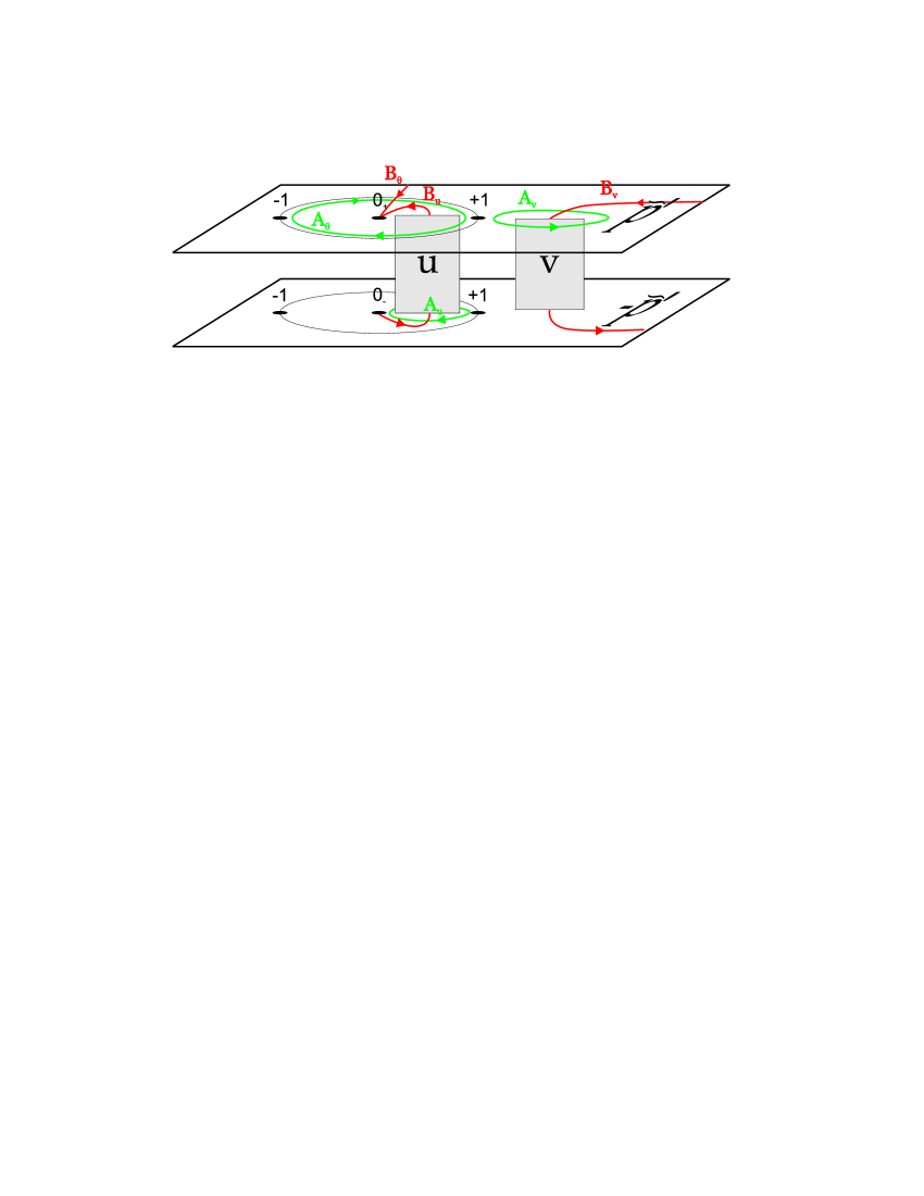
Figure 1: Algebraic curve from the finite gap method. $u$ and $v$ cuts correspond to cuts inside and outside the unit circle respectively.

If we are looking for a finite gap solution the number $K$ of these cuts is finite and we conclude that $\tilde{p}^{\prime}(x),-\tilde{p}^{\prime}(x)$ are two branches of an analytical function defined by a hyperelliptic curve (see fig.1),

$$(p^{\prime})^{2}=\frac{P^{2}(x)}{Q(x)},$$ (14)

where $Q(x)$ has $2K$ zeros and the order of $P(x)$ is fixed by the large $x$ asymptotics eq.(11). We denote the branch cuts of $p^{\prime}(x)$ by $u$ ($v$) cuts if they are inside (outside) the unit circle. These cuts are the loci where the eigenvalues of the monodromy matrix become degenerate. Thus, when crossing such cut the quasi-momentum may at most jump by a multiple of $2\pi$ which characterizes each cut,

$$\tilde{p}/(x)=\pi n_{k},\qquad x\in{\cal C}_{k}$$ (15)

where $\tilde{p}/(x)$ is the average of the quasi-momentum above and below the cut,

$$\tilde{p}/(x)\equiv\frac{1}{2}\left(\tilde{p}(x+i0)+\tilde{p}(x-i0)\right)\,.$$ (16)

Each cut is also parameterized by the filling fraction numbers which we define as integrals along $A$-cycles of the curve (see fig.1)

$$S_{i}^{v}=-\frac{\sqrt{\lambda}}{8\pi^{2}i}\oint_{A^{v}_{i}}\tilde{p}(x)\left(1-\frac{1}{x^{2}}\right)dx,\;\;\;\;\;S_{i}^{u}=\frac{\sqrt{\lambda}}{8\pi^{2}i}\oint_{A^{u}_{i}}\tilde{p}(x)\left(1-\frac{1}{x^{2}}\right)dx\,.$$ (17)

Finally, imposing (15,17,9,10,11) one fixes completely the undetermined constants in (14).

2 Quantum Bethe Ansatz and Classical Limit: $O(4)$ Sigma-Model

We will describe a quantum state of the $O(4)$ sigma model by a system of $L$ relativistic particles of mass $\mu/2\pi$ put on a circle of the length $2\pi$. The momentum and the energy of each particle can be suitably parametrized by its rapidity as $p=\frac{\mu}{2\pi}\sinh\theta$ and $e=\frac{\mu}{2\pi}\cosh\theta$ so that the total energy and momentum will be given by

$$P = \frac{\mu}{2\pi}\sum\limits_{{\alpha}=1}^{L}\sinh(\pi\theta_{\alpha})\,,$$ (18)

$$E = \frac{\mu}{2\pi}\sum\limits_{{\alpha}=1}^{L}\cosh(\pi\theta_{\alpha})\,.$$ (19)

These particles transform in the vector representation under $O(4)$ symmetry group or in the bi-fundamental representations of $SU(2)_{R}\times SU(2)_{L}$. The scattering of the particles in this theory is known to be elastic and factorizable: the relativistic S-matrix $\hat{S}\left(\theta_{1}-\theta_{2}\right)$ depends only on the difference of rapidities of scattering particles $\theta_{1}$ and $\theta_{2}$ and obeys the Yang–Baxter equations. As was shown in [5] (and in [7, 9, 23, 24] for the general principle chiral field) these properties, together with the unitarity and crossing-invariance, define essentially unambiguously the S-matrix $\hat{S}$. Let us recall briefly how the bootstrap program goes. From the symmetry of the problem we know that

$$\hat{S}=\hat{S}_{L}\times\hat{S}_{R}$$ (20)

where $S_{L,R}$ are built by use of the two $SU(2)$ invariant tensors and can therefore be written as

$$S_{R,L}(\theta)^{a^{\prime}b^{\prime}}_{a\,b}=\frac{S_{0}(\theta)}{\theta-i}\left(\theta\,\delta^{a^{\prime}}_{a}\delta^{b^{\prime}}_{b}-i\,f(\theta)\,\delta^{b^{\prime}}_{a}\delta^{a^{\prime}}_{b}\right)\,.$$

Imposing the Yang-Baxter equation on $\hat{S}$ yields $f(\theta)=1$, while the unitarity constrains the remaining unknown function to obey

$$S_{0}(\theta)S_{0}(-\theta)=1\,$$ (21)

and crossing symmetry requires

$$S_{0}(\theta)=\left(1-\frac{i}{\theta}\right)S_{0}(i-\theta)\,.$$ (22)

From (21), (22) and the absence of poles on the physical strip $0<\theta<2$ one can compute the scalar factor: $S_{0}(\theta)=\frac{\Gamma\left(-\frac{\theta}{2i}\right)\Gamma\left(\frac{1}{2}+\frac{\theta}{2i}\right)}{\Gamma\left(\frac{\theta}{2i}\right)\Gamma\left(\frac{1}{2}-\frac{\theta}{2i}\right)}$. For our purpose we just need the much easier to extract large $\theta$ asymptotics,

$$i\log S^{2}_{0}(\theta)\sim 1/\theta+O(1/\theta^{3})\,.$$ (23)

2.1 Bethe Equations for Particles on a Circle

When this system of particles is put into a finite 1-dimensional periodic box of the length $\cal L$ the set of rapidities of the particles $\{\theta_{\alpha}\}$ is constrained by the condition of periodicity of the wave function $|\psi\rangle$ of the system,

$$|\psi\rangle=e^{i\mu\sinh\pi\theta_{\alpha}}\overleftarrow{\prod_{1}^{{\alpha}-1}}\ \hat{S}\left(\theta_{\alpha}-\theta_{\beta}\right)\overrightarrow{\prod_{N}^{{\alpha}+1}}\ \hat{S}\left(\theta_{\alpha}-\theta_{\beta}\right)|\psi\rangle$$ (24)

where the first term is due to the free phase of the particle and the second is the product of the scattering phases with the other particles. The arrows stand for ordering of the terms in the product and $\mu=m_{0}{\cal L}$ is a dimensionless parameter. Diagonalization of both the L and R factors in the process of fixing the periodicity (24) leads to the following set of Bethe equations [25] which may be found from eq.(24) by the algebraic Bethe ansatz method [26, 27]

$$2\pi m_{\alpha} = \mu\sinh\pi\theta_{\alpha}-\sum_{\beta\neq\alpha}^{L}\,i\log S_{0}^{\,2}\left(\theta_{\alpha}-\theta_{\beta}\right)$$ (25)

$$- \sum_{j}^{J_{u}}i\log\frac{\theta_{\alpha}-u_{j}+i/2}{\theta_{\alpha}-u_{j}-i/2}\,-\sum_{k}^{J_{v}}i\log\frac{\theta_{\alpha}-v_{k}+i/2}{\theta_{\alpha}-v_{k}-i/2}\,,$$

$$2\pi n_{j}^{u} = \sum_{\beta}^{L}i\log\frac{u_{j}-\theta_{\beta}-i/2}{u_{j}-\theta_{\beta}+i/2}+\sum_{i\neq j}^{J_{u}}i\log\frac{u_{j}-u_{i}+i}{u_{j}-u_{i}-i}\,,$$ (26)

$$2\pi n_{j}^{v} = \sum_{\beta}^{L}i\log\frac{v_{k}-\theta_{\beta}-i/2}{v_{k}-\theta_{\beta}+i/2}+\sum_{l\neq k}^{J_{v}}i\log\frac{v_{k}-v_{l}+i}{v_{k}-v_{l}-i}\,,$$ (27)

where $u$’s and $v$’s are the Bethe roots appearing from the diagonalization of (24) and characterizing each quantum state. A quantum state with no such roots corresponds to the highest weight ferromagnetic state where all spins of both kinds are up. Adding a $u$ ($v$) roots corresponds to flipping one of the right (left) $SU(2)$ spins, thus creating a magnon. The left and right charges of the wave function, associated with the two $SU(2)$ spins are given by

$$Q_{L}=L-2J_{u}\,,\qquad Q_{R}=L-2J_{v}\,.$$ (29)

This model with massive relativistic particles and the asymptotically free UV behavior cannot look like a consistent quantum string theory. Only in the classical limit we can view it as a string toy model obeying the classical conformal symmetry. In the classical case it is also easy to impose the Virasoro conditions. In the quasi-classical limit , we still can try to impose the Virasoro conditions as some natural constraints on the quantum states. We will discuss this point latter.

2.2 Quasi-classical limit

In the classical limit the physical mass of the particle

$$\frac{\mu}{2\pi}\sim e^{-\sqrt{\lambda}/2}\,,$$ (30)

where $\lambda$ is the physical coupling at the scale $2\pi$, vanishes since $\lambda\rightarrow\infty$. Moreover we should focus on quantum states with large quantum numbers, i.e. we shall consider a large number $L\to\infty$ of particles on the ring.

Let us now think of (25-27) as of the equations for the equilibrium condition for a system of three kinds of particles: ($\theta_{\alpha}$, $u_{j}$ and $v_{k}$), interacting between themselves and experiencing the external constant forces ($2\pi m_{\alpha}$, $2\pi n_{j}^{u}$ and $2\pi n_{k}^{v}$). The particles of the $\theta$ kind are also placed into the external confining potential

$$V(z)=\mu\cosh(\pi Mz)\,\,,\,\,\qquad z=\theta/M$$ (31)

where

$$M\equiv-\frac{\log\mu}{2\pi}\simeq\frac{\sqrt{\lambda}}{4\pi}\,.$$ (32)

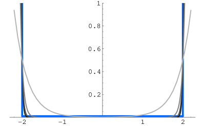
Figure 2: We plot $V(z)$ for $M=1,5,9,13$ (lighter to darker gray). It is clear that the potential approaches the blue box potential as $M\rightarrow\infty$.

In the classical limit the potential becomes a square box potential with the infinite walls at $z=\pm 2$ (see fig.2). Moreover, since this is a large box for the original variables we can use the asymptotics (23) for the force between particles of the $\theta$ (or $z$) type. The box potential provides the appropriate boundary conditions for the density of particles interacting by the Coulomb force. Since they repeal each other the density should be peaked around $z=\pm 2$. To find the correct asymptotics close to these two points, we can consider eq.(25) as the equilibrium condition for the gas of Coulomb particles in the box.

If the right and left modes (magnons) are not excited we have only the states with $U(1)$ modes. In the classical limit, using the Coulomb approximation eq.(23), we have for this sector the following Bethe equation

$$\mu\sinh\pi Mz_{\alpha}-2\pi\,m = -\frac{1}{M}\sum_{\beta\neq\alpha}^{L}\frac{1}{z_{{\alpha}}-z_{\beta}}\,.$$

In the continuous limit, the equation for the asymptotic density, $L\sim M\rightarrow\infty$, is given, through the resolvent $G_{\theta}(z)=\frac{1}{M}\sum_{\beta=1}^{L}\frac{1}{z-z_{\beta}}$ by

$$\,/\!\!\!\!G_{\theta}(z)=-2\pi m,\;\;\;\;\;\,z\in\mathcal{C}_{\theta}\,,$$ (33)

with inverse square root boundary conditions near $\pm 2$. The analytical function $G_{\theta}(x)$ having a real part on the cut defined by eq.(33), with support $[-2,2]$, with inverse square root boundary conditions (the only compatible with the asymptotics at $z\to\infty$: $G_{\theta}(z)\to\frac{L}{M}\frac{1}{z}$, is completely fixed:

$$G_{\theta}(z)=\left(\frac{2\pi m\ z+\frac{L}{M}}{\sqrt{z^{2}-4}}-2\pi m\right),\qquad L>4\pi|m|M$$ (34)

which gives for the density

$$\rho_{\theta}(z)=\frac{1}{\pi}\left(\frac{2\pi m\ z+\frac{L}{M}}{\sqrt{4-z^{2}}}\right)\,.$$ (35)

For a general solution with $u$ and $v$ magnons we will also find the same asymptotics

$$\rho(z)\equiv\frac{1}{M}\sum_{\alpha=1}^{L}\delta\left(z-z_{\alpha}\right)\simeq\frac{2\kappa_{\pm}}{\sqrt{2\mp z}},\qquad z\to\pm 2.$$ (36)

with $\kappa_{\pm}$ yet to be determined through the energy and momentum of the solution, as we shall explain in the next section.

We will be considering the scenario where we have the same mode number $m_{\alpha}=m$ for all $z$ particles. As proposed in [2, 16] this is the adequate set of states which will obey the Virasoro constraints in the classical limit.

First, we will relate the $z$ behavior close to the walls, characterized by the constants $\kappa_{\pm}$ with the energy and momentum $E,P$ of the quantum state, as given by (37,19). Then we shall eliminate the $\theta$’s from the system of Bethe equations by explicitly solving the first one in the considered limit. Finally, we will justify why we take the same mode number $m$ for all $\theta$’s by identifying the longitudinal modes to the excited mode numbers $m_{i}$ in the Bethe ansatz setup. This constraint on the states will correspond to the Virasoro conditions, at least in the classical limit.

2.2.1 Energy and momentum

The total momentum can be calculated exactly, before any classical limit

$$P=\frac{\mu}{2\pi}\sum_{{\alpha}}\sinh(\pi\theta_{\alpha})=m_{p}L_{p}-\sum_{p}n_{p}S_{p}^{u}-\sum_{p}n_{p}S_{p}^{v}$$ (37)

where $L_{p},S_{p}^{u},\;S_{p}^{v}$ are the filling fractions, or the numbers of Bethe roots with a given mode numbers $m_{p},n_{u,p},n_{v,p}$. To prove this, it suffices to sum the eq.(25) for all roots $\theta_{\alpha}$. The contribution of $S_{0}(\theta)$ terms cancels due to antisymmetry while the second and third sums in the r.h.s. of (25) are replaced using (26) and (27), respectively.

Let us show how to calculate the energy (19) which is a fare less trivial task [2]. As a byproduct we will also reproduce the total momentum from the behavior at the singularities at $z=\pm 2$ described by the residua $\kappa_{\pm}$. We want to compute the sum

$$E\equiv\frac{\mu}{2\pi}\sum_{\alpha}\cosh(\pi\theta_{\alpha})\,,$$

but we cannot simply replace this sum by an integral and use the asymptotic density $\rho_{\theta}(z)$ to compute the energy. That is because the main contribution to the energy comes from large $\theta$’s, near the walls, where the expression for the asymptotic density is no longer accurate. It is natural for the classical limit since the particles become effectively massless and the contributions of right and left modes are clearly distinguishable and located far from $\theta=0$. We notice that the energy is dominated by large $\theta$’s where, with exponential precision, we can replace $\cosh\pi\theta_{\alpha}$ by $\pm\sinh\pi\theta_{\alpha}$ for positive (negative) $\theta_{\alpha}$. Furthermore, the contribution from the $\theta$’s in the middle of the box is also exponentially suppressed since $\mu$ is very small. Thus we can pick a point $a$ somewhere in the box not too close to the walls. One can think of $a$ as being somewhere in the middle. Then,

$$E=\sum_{z_{\alpha}>a}\frac{\mu}{2\pi}\sinh\left(\pi z_{\alpha}M\right)-\sum_{z_{\alpha}<a}\frac{\mu}{2\pi}\sinh\left(\pi z_{\alpha}M\right)\,,$$

where, let us stress, the result is correct independently of the point $a$ within the interval $-2<a<2$ with the exponential precision. Each sum of $\sinh\pi\theta_{\alpha}$ can be substituted by the corresponding r.h.s. of the Bethe equation (25), thus giving

$$E \simeq \frac{i}{\pi}\!\!\!\!\sum_{z_{\beta}<a<z_{\alpha}}\!\!\!\!\log S_{0}^{2}\left(M\left[z_{\alpha}-z_{\beta}\right]\right)+\sum_{\alpha}m\;{\rm sign}(z_{\alpha}-a)\,$$

$$- \frac{1}{2\pi}\sum_{j,\alpha}{\rm sign}(z_{\alpha}-a)i\log\frac{Mz_{\alpha}-u_{j}+i/2}{Mz_{\alpha}-u_{j}-i/2}-\frac{1}{2\pi}\sum_{k,\alpha}{\rm sign}(z_{\alpha}-a)i\log\frac{Mz_{\alpha}-v_{k}+i/2}{Mz_{\alpha}-v_{k}-i/2}$$

As mentioned above we assume all $m_{\alpha}$ to be the same . Now we can safely go to the continuous limit since in the first term the distances between $z$’s are now mostly of the order $1$. This allows to rewrite the energy, with $1/M$ precision, as follows

$$E \simeq -\frac{M}{\pi}\int_{-2}^{a}dz\int_{a}^{2}dw\frac{\rho_{\theta}(z)\rho_{\theta}(w)}{z-w}-\frac{M}{2\pi}\int\frac{\rho_{\theta}(z)\rho_{u}(w)}{z-w}{\rm sign}(z-a)\,dz\,dw$$ (39)

$$- \frac{M}{2\pi}\int\frac{\rho_{\theta}(z)\rho_{v}(w)}{z-w}{\rm sign}(z-a)\,dz\,dw+m\,M\int\rho_{\theta}(z){\rm sign}(z-a)\,dz$$

where we are now free to use the asymptotic density $\rho_{\theta}(z)$. By the use of Bethe equations, we managed to transform the original sum over $\cosh$’s, highly peaked at the walls, into a much smoother sum where the main contribution is now softly distributed along the bulk and where the continuous limit does not look suspicious. From the previous discussion we know that this expression does not depend on $a$ provided $a$ is not too close to the walls. In fact, we can easily see that it does not depend on $a$ at all after taking the continuous limit leading to the perfect box-like potential. To prove it one notices that due to Bethe equations eq.(25) the $a$-derivative of eq.(39) is zero for all $a\in]-2,2[$. Hence we can even send $a$ close to a wall: $a=-2+\epsilon$, where $\epsilon$ is very small. But then the last three terms in (39) are precisely the momentum (37), as explained in the beginning of this section. To compute the first term we can now use the asymptotics (23,36). The contribution of this term is then given by

$$-\frac{M}{\pi}\int_{-2}^{-2+\epsilon}dz\int_{-2+\epsilon}^{2}dw\frac{\rho_{\theta}(z)\rho_{\theta}(w)}{z-w}\simeq-\int_{-2}^{-2+\epsilon}dz\int_{-2+\epsilon}^{2}dw\frac{4M\kappa_{-}^{2}}{\pi(z-w)\sqrt{2+z}\sqrt{2+w}}\simeq 2\pi M\kappa_{-}^{2}$$

so that

$$E\simeq 2M\kappa_{-}^{2}\pi+P\,.$$ (40)

If we compute the $a$-independent integral (39) near the other wall, i.e. for $a=2-\epsilon$, we find

$$E\simeq 2M\kappa_{+}^{2}\pi-P\,.$$

Therefore, equating the results one obtains the desired expressions for the energy and momentum

$$E\pm P=2\pi\,M\,\kappa_{\pm}^{2}$$ (41)

through the singularities of the density of rapidities at $z=\pm 2$, described by $\kappa_{\pm}$. Together with (32) this is precisely the classical formula (5).

2.2.2 Elimination of $\theta$’s and AFS equations

It is useful for what follows, to introduce some new notations. Using the Zhukovsky map

$$z=x(z)+\frac{1}{x(z)}\,\,,\,\,|x(z)|>1$$ (42)

we define

$$y_{j}^{\,\pm}\equiv x\left(\frac{u_{j}\pm\,i/2}{M}\right),\;\;\;\;\;y_{j}\equiv x\left(\frac{u_{j}}{M}\right)$$

with the similar expressions for $v_{l}$ given by $\tilde{y}_{l}^{\pm}$ and $\tilde{y}_{l}$.

In this section, for the purposes of comparison with the asymptotic AFS Bethe ansatz for the N=4 SYM theory, let drop the $v$ magnons, $J_{v}=0$. Their contributions will be easily restored later. As explained at the beginning of this section we can write the first Bethe equation, (25) as

$$-\hskip-11.66573pt\int_{-2}^{2}\frac{\rho(w)}{z-w}dw=-\sum_{j}^{J_{u}}i\log\frac{Mz-u_{j}+i/2}{Mz-u_{j}-i/2}-2\pi m,\,\,\,\,z\in[-2,2]\,.$$

The solution to this Riemann-Hilbert problem with the boundary conditions and the normalization given by (36) looks as follows [3]

$$\rho(z) = \frac{1}{\pi\sqrt{4-z^{2}}}\left[\left(2\pi m+i\sum\limits_{j=1}^{J_{u}}\log\frac{y_{j}^{-}}{y_{j}^{+}}\right)\,z+\frac{L}{M}+2i\sum\limits_{j=1}^{J_{u}}\left(\frac{1}{y_{j}^{+}}-\frac{1}{y_{j}^{-}}\right)\right]$$ (43)

$$- \frac{1}{\pi}\sum\limits_{j=1}^{J_{u}}\log\left(\frac{x(z)y_{j}^{+}-1}{x(z)y_{j}^{-}-1}\,\,\,\,\frac{x(z)-y_{j}^{-}}{x(z)-y_{j}^{+}}\right)\ .$$

We want to focus on such states that the momentum $P$ related to the asymptotics close to the walls by (41), vanishes. Thus we should set to zero the first term in the r.h.s. of eq.(43):

$$P=m-\frac{i}{2\pi}\sum\limits_{j=1}^{J_{u}}\log\frac{y_{j}^{+}}{y_{j}^{-}}=0\,.$$ (44)

Then, plugging this density into (26), integrating over the rapidities and exponentiating the result, we find [3]

$$\left(\frac{y_{k}^{+}}{y_{k}^{-}}\right)^{L}=\prod_{j\neq k}^{J_{u}}\frac{u_{k}-u_{j}+i}{u_{k}-u_{j}-i}\,\sigma^{2}(u_{j},u_{k})\,,$$ (45)

where the “dressing” factor $\sigma^{2}$ is given by

$$\sigma^{2}(u_{j},u_{k})=\left(\frac{1-1/(y_{j}^{-}y_{k}^{+})}{1-1/(y_{j}^{+}y_{k}^{-})}\right)^{-2}\left(\frac{y_{j}^{-}y_{k}^{-}-1}{y_{j}^{-}y_{k}^{+}-1}\frac{y_{j}^{+}y_{k}^{+}-1}{y_{j}^{+}y_{k}^{-}-1}\right)^{2i(u_{j}-u_{k})}\,.$$ (46)

These are precisely the AFS equations conjectured in [19] as the asymptotic Bethe ansatz equation for the $SU(2)$ sector of $N=4$ SYM theory . The dispersion relation for these dressed magnons can be read off from the asympotics of the density eq.(43) close to the walls

$$\Delta\equiv\sqrt{\lambda}\,\kappa=L+2Mi\sum\limits_{j=1}^{J_{u}}\left(\frac{1}{y_{j}^{+}}-\frac{1}{y_{j}^{-}}\right)\,.$$ (47)

2.2.3 Classical limit and KMMZ algebraic curve

To consider the classical limit we trivially restore the $v$ roots from the previous calculation, to find

$$\left(\frac{y_{k}^{+}}{y_{k}^{-}}\right)^{L} = \prod_{j\neq k}^{J_{u}}\frac{u_{k}-u_{j}+i}{u_{k}-u_{j}-i}\,\sigma^{2}(u_{j},u_{k})\,\prod_{l=1}^{J_{v}}\sigma^{2}(v_{l},u_{k})\,,$$ (48)

and similarly for $\tilde{y}_{k}$, and consider the limit where $J_{u},J_{v},L\sim M$, so that the $u$ and $v$ roots also scale as $M$. Then the expansion of this equation, after taking the $\log$’s, gives to the leading order in $1/M$

$$\pi n_{k} = \frac{\frac{L}{2M}y_{k}+2\pi m}{1-y_{k}^{2}}+\frac{1}{y_{k}^{2}-1}\frac{1}{M}\sum_{l=1}^{J_{v}}\frac{1}{1/y_{k}-\tilde{y}_{l}}+\frac{y^{2}_{k}}{y^{2}_{k}-1}\frac{1}{M}\sum_{j\neq k}^{J_{u}}\frac{1}{y_{k}-y_{j}}\,.$$ (49)

Finally we can define the quasimomentum [3]

$$p(x)=\frac{\frac{L}{2M}x+2\pi m}{1-x^{2}}+\frac{1}{x^{2}-1}\frac{1}{M}\sum_{j=1}^{J_{v}}\frac{1}{1/x-\tilde{y}_{j}}+\frac{x^{2}}{x^{2}-1}\frac{1}{M}\sum_{j=1}^{J_{u}}\frac{1}{x-y_{j}}\,.$$ (50)

Let us explain how it becomes precisely the quasimomentum we had in the context of the algebraic curve in section 1.2 in the classical theory. It is clear that we indeed have the asymptotics (10,11) close to $x=0,\infty$. Then, to relate the residues of eq.(50) to the ones found from the algebraic curve in eq.(9), we expand (47) in our limit as follows:

$$\Delta=L+\sum_{j}\frac{2}{y_{j}^{2}-1}+\sum_{l}\frac{2}{\tilde{y}_{l}^{2}-1}$$ (51)

and check that this is indeed what one finds from the quasimomenta we just defined. Finally, when we consider a large number of magnons $J_{u},J_{v}$ the roots in eq.(50) condense into a number of one dimensional supports, the sums becoming the integrals along these lines giving the same square root cuts as we had in the finite gap construction.

2.2.4 Geometric proof

The roots solving (25,26,27) with the same mode number will condense into a single square root cut. When we consider more than one type of mode numbers we see that the particles condense into a few distinct supports, one for each distinct mode number

$$\mathcal{C}=\mathcal{C}_{1}\cup\dots\cup\mathcal{C}_{K}\,.$$

We can now rescale the Bethe roots

$$(u,v,\theta)=M(x,y,z)$$ (52)

and define

$$p_{1}=-p_{2} = \frac{1}{M}\sum_{i=1}^{J_{u}}\frac{1}{z-x_{i}}-\frac{1}{2M}\sum_{\beta=1}^{L}\frac{1}{z-z_{\beta}}$$

$$p_{3}=-p_{4} = \frac{1}{M}\sum_{l=1}^{J_{v}}\frac{1}{z-y_{l}}-\frac{1}{2M}\sum_{\beta=1}^{L}\frac{1}{z-z_{\beta}}\,.$$ (53)

Then we can recast the Bethe equations in this scaling limit as follows

$$x\in{\cal C}_{u}, \;\;\;\;\;{p_{1}}^{+}-{p_{2}}^{-}=2\pi n_{u}$$

$$x\in{\cal C}_{\theta}, \;\;\;\;\;{p_{2}}^{+}-{p_{3}}^{-}=2\pi m$$ (54)

$$x\in{\cal C}_{v}, \;\;\;\;\;{p_{3}}^{+}-{p_{4}}^{-}=2\pi n_{v}$$

$$x\in{\cal C}_{\theta}, \;\;\;\;\;{p_{4}}^{+}-{p_{1}}^{-}=2\pi m,$$

where we

• considered, as in the preceding section, one single mode number $m$ for all rapidities;

• dropped the momentum $\mu\sinh\theta$. As we explained in section 2.2 we can do this provided we replace it by the boundary conditions (36).

These equations tell us that $p^{\prime}_{1}(z),p^{\prime}_{2}(z),p^{\prime}_{3}(z),p^{\prime}_{4}(z)$ form four sheets of the Riemann surface of an analytical function $p^{\prime}(z)$ (see fig.3).

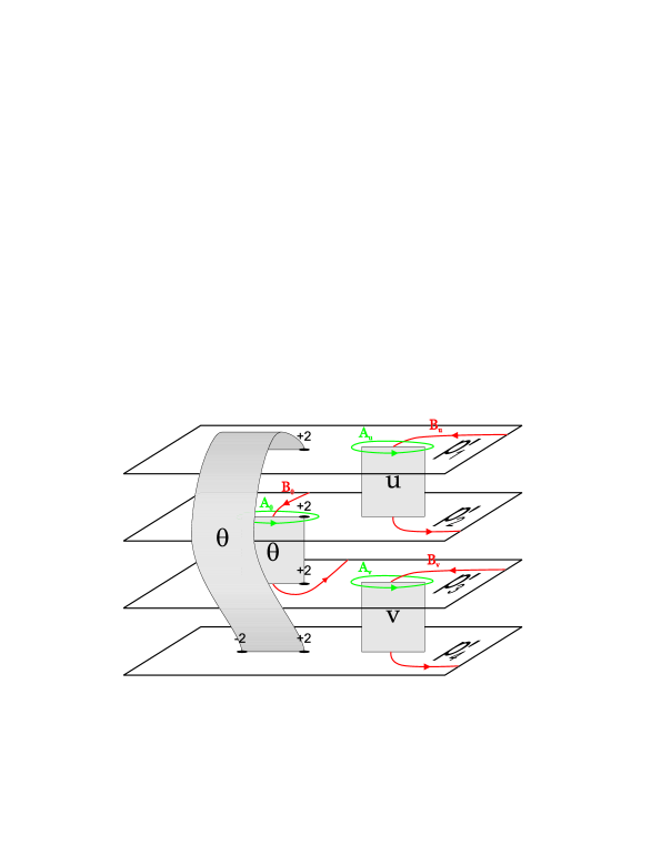
Figure 3: Structure of the curve coming from the Bethe ansatz side. This figure is related with fig.1 by means of the Zhukovsky map.

They can also be written as holomorphic integrals around the infinite B-cycles:

$$\oint_{B^{u}_{j}}dp = 2\pi n_{u,j}\qquad n_{j}=1,\ldots,K_{u}$$

$$\oint_{B^{v}_{j}}dp = 2\pi n_{v,j}\qquad n_{j}=1,\ldots,K_{v}$$ (55)

$$\oint_{B^{\theta}}dp = 2\pi m$$

where the the first two conditions correspond to the equations in the first and third line of (54), respectively, while the last one corresponds to any of the equations of the second and fourth lines of (54). The $B$ cycles are defined as in fig.3.

We found two Riemann surfaces which we plotted in figures 1 and 3. The equivalence between these two curves is achieved through the Zhukovsky map [2]

$$z=x+\frac{1}{x}$$

and amounts to the equivalence between the finite gap solutions for the classical theory and the Bethe ansatz solutions in the scaling limit.

2.2.5 Virasoro modes

We established the equivalence between

• all classical solutions following from the PCF action (1) and subject to the Virasoro conditions ${\rm tr}\left(j_{\tau}\pm j_{\sigma}\right)^{2}=-2\kappa_{\pm}^{2}$ as described by the construction of the algebraic curve of section 1.2.

• and the Bethe ansatz quantum solution (25-26) in the scaling limit (52) with all rapidities $\theta_{\alpha}$ having the same mode number $m$.

In the context of string theory one is interested in quantizing the Polyakov string action

$$S=\frac{\sqrt{\lambda}}{8\pi}\int d\sigma d\tau\sqrt{h}\,h^{ab}\left({\rm tr}\,\partial_{a}g^{\dagger}\partial_{b}g-\partial_{a}Y\partial_{b}Y\right)\,.$$ (56)

Due to its local reparametrization and Weyl symmetries one can then fix the target space time $Y$ as in (4) and reduce the action to (1). However, due to the residual reparametrization symmetry

$$\tau\pm\sigma\rightarrow f_{\pm}(\tau\pm\sigma)\,,$$ (57)

one must keep in mind that the original presence of the world-sheet metric field imposes that the stress energy tensor vanishes. This is precisely the Virasoro conditions.

On the other hand, from the field theory point of view the Bethe ansatz equations (25-27) should describe all possible states of the theory, not only those for which

$$\langle\psi|T^{ab}|\phi\rangle=0\,.$$ (58)

Thus, in view of the equivalence we proved, we are lead to the conclusion that if we start with some classical solution with one $\theta$ cut and some $u$ and $v$ cuts, the excitation of additional microscopic $\theta$ cuts should correspond to the inclusion of the longitudinal modes which we drop in the context of string theory. Indeed, these massless (from the world-sheet point of view) excitations coming from our conformal gauge choice, appear if one expands the action around the classical solution without fixing the Virasoro conditions from the beginning (see for instance expression 2.7 and the discussion following it in [31]). In this section we verify this claim therefore justifying this single $\theta$ cut restriction, first proposed in [16] and given the interpretation as the Virasoro condition in [2].

In (2.2.1) we computed the energy of a quantum state where all mode numbers $m_{\alpha}=m$ were the same. If we change the mode numbers of a few $\theta$’s we will have a macroscopic support with particles having the mode number $m$ surrounded by some microscopic domains, linear supports, with mode numbers $m_{\beta}<m$ (to the left of it) and $m_{\beta}>m$ (to its right).

Let us assume that we excite them one at a time and focus on the first particle whose mode number we change. Before we do it, it is in equilibrium due to the exponential force exerted by the wall of the box (31) and by (an equal) force produced by all the other particles and by the constant force $2\pi m$ – see (25). When we change the particle mode number the constant force increases pushing the particle against the wall. However since the forces are exponential the shift will be very small, much smaller than $1/M$ - the characteristic distance between the neighboring rapidities. Then let us consider the particles in the middle of the box, the ones whose position is well described by the asymptotic density $\rho(z)$. They only feel the change in mode number through the new position of the corresponding $\theta$ particle. Since this shift is very small the asymptotic density, to the order we are interested, is not changed. Thus, in this procedure of changing a few mode numbers we conclude that, when going to the continuous limit in (2.2.1), only the second term will lead to a different result so that

$$\delta E=\sum_{n}|n|N_{m+n}$$ (59)

where $N_{n}$ is the number of particles with mode number $n$. We found in this way the massless (world-sheet) modes associated with the local reparametrization symmetry of the world-sheet. These modes appear when considering the fluctuations around a classical solution [31] and are the only ones not taken into account by the finite gap algebraic curve [20].

- [1] V. A. Kazakov, A. Marshakov, J. A. Minahan and K. Zarembo, “Classical / quantum integrability in AdS/CFT,” JHEP 0405 (2004) 024 [arXiv:hep-th/0402207].
- [2] N. Gromov, V. Kazakov, K. Sakai and P. Vieira, “Strings as multi-particle states of quantum sigma-models,” Nucl. Phys. B 764 (2007) 15 [arXiv:hep-th/0603043].
- [3] N. Gromov and V. Kazakov, “Asymptotic Bethe ansatz from string sigma model on ,” arXiv:hep-th/0605026.
- [4] S. Novikov, S. V. Manakov, L. P. Pitaevsky and V. E. Zakharov, “Theory Of Solitons. The Inverse Scattering Method,” Consultants Bureau, New York and London, 1984.
- [5] A. B. Zamolodchikov and A. B. Zamolodchikov, “Relativistic Factorized S Matrix In Two-Dimensions Having O(N) Isotopic Symmetry,” Nucl. Phys. B 133 (1978) 525 [JETP Lett. 26 (1977) 457].
- [6] A.M. Polyakov, P.B. Wiegmann, ”Theory of Non-Abelian Goldstone Bosons”, Phys.Lett.131B (1984) 121.
- [7] P. B. Wiegmann, “Exact Solution For The SU(N) Main Chiral Field In Two-Dimensions,” JETP Lett. 39 (1984) 214 [Pisma Zh. Eksp. Teor. Fiz. 39 (1984) 180].
- [8] L. D. Faddeev and N. Y. Reshetikhin, “Integrability Of The Principal Chiral Field Model In (1+1)-Dimension,” Annals Phys. 167 (1986) 227.
- [9] P. Wiegmann, “Exact Factorized S Matrix Of The Chiral Field In Two-Dimensions,” Phys. Lett. B 142, 173 (1984).
- [10] V.A. Fateev, V.A. Kazakov, P.B. Wiegmann, ”Principal chiral field at large N”, Nucl. Phys. B424 [FS] (1994) 505-520, [arXiv:hep-th/9403099].
- [11] J. Balog, S. Naik, F. Niedermayer, P. Weisz, Phys.Rev.Lett. 46 (1992). 356.
- [12] N. Reshetikhin and F. Smirnov “Quantum Floquet functions”, Zapiski nauchnikh seminarov LOMI (Notes of scientific seminars of Leningrad Branch of Steklov Institute) v.131 (1983) 128 (in russian).
- [13] N. Beisert, J. A. Minahan, M. Staudacher and K. Zarembo, “Stringing spins and spinning strings”, JHEP 0309, 010 (2003) [arXiv:hep-th/0306139].
- [14] B. Sutherland, “Low-Lying Eigenstates of the One-Dimensional Heisenberg Ferromagnet for any Magnetization and Momentum”, Phys. Rev. Lett. 74, 816 (1995).
- [15] G. P. Korchemsky, “WKB quantization of reggeon compound states in high-energy QCD,” arXiv:hep-ph/9801377.
- [16] N. Mann and J. Polchinski, “Bethe ansatz for a quantum supercoset sigma model,” Phys. Rev. D 72 (2005) 086002 [arXiv:hep-th/0508232].
- [17] N. Beisert, V. A. Kazakov and K. Sakai, “Algebraic curve for the SO(6) sector of AdS/CFT,” Phys. Rev. D 71 (2005) 125019 [arXiv:hep-th/0504024].
- [18] G. Arutyunov, S. Frolov and M. Staudacher, “Bethe ansatz for quantum strings,” JHEP 0410 (2004) 016 [arXiv:hep-th/0406256].
- [19] L. F. Alday, G. Arutyunov and S. Frolov, “New integrable system of 2dim fermions from strings on ,” JHEP 0601 (2006) 078 [arXiv:hep-th/0508140]; G. Arutyunov and S. Frolov, “Uniform light-cone gauge for strings in : Solving sector,” JHEP 0601 (2006) 055 [arXiv:hep-th/0510208].
- [20] N. Gromov and P. Vieira, to appear
- [21] N. Beisert, V. A. Kazakov, K. Sakai and K. Zarembo, “Complete spectrum of long operators in N = 4 SYM at one loop,” JHEP 0507 (2005) 030 [arXiv:hep-th/0503200].
- [22] N. Dorey and B. Vicedo, “On the dynamics of finite-gap solutions in classical string theory,” arXiv:hep-th/0601194.
- [23] P. B. Wiegmann, “On The Theory Of Nonabelian Goldstone Bosons In Two-Dimensions: Exact Solution Of The O(3) Nonlinear Sigma Model,” Phys. Lett. B 141, 217 (1984).
- [24] E. Ogievetsky, N. Reshetikhin and P. Wiegmann, “The Principal Chiral Field In Two-Dimension And Classical Lie Algebra,” NORDITA-84/38
- [25] A. B. Zamolodchikov and A. B. Zamolodchikov, “Massless factorized scattering and sigma models with topological terms,” Nucl. Phys. B 379 (1992) 602.
- [26] L. D. Faddeev, E. K. Sklyanin and L. A. Takhtajan, “The Quantum Inverse Problem Method. 1,” Theor. Math. Phys. 40, 688 (1980) [Teor. Mat. Fiz. 40, 194 (1979)].
- [27] P. P. Kulish, N. Y. Reshetikhin and E. K. Sklyanin, “Yang-Baxter Equation And Representation Theory: I,” Lett. Math. Phys. 5, 393 (1981).
- [28] H. Bethe, ”On the Theory of Metals. 1. Eigenvalues and Eigenfunctions for the linear atomic chain”, Z.Phys. 71 (1931) 205.
- [29] J. A. Minahan, “The SU(2) sector in AdS/CFT,” Fortsch. Phys. 53, 828 (2005) [arXiv:hep-th/0503143].
- [30] A. Rej, D. Serban and M. Staudacher, “Planar N = 4 gauge theory and the Hubbard model,” arXiv:hep-th/0512077.
- [31] S. Frolov and A. A. Tseytlin, “Quantizing three-spin string solution in ,” JHEP 0307 (2003) 016 [arXiv:hep-th/0306130].