Ellipsoidal universe in the brane world

Abstract

We study a scenario of the ellipsoidal universe in the brane world cosmology with a cosmological constant in the bulk . From the five-dimensional Einstein equations we derive the evolution equations for the eccentricity and the scale factor of the universe, which are coupled to each other. It is found that if the anisotropy of our universe is originated from a uniform magnetic field inside the brane, the eccentricity decays faster in the bulk in comparison with a four-dimensional ellipsoidal universe. We also investigate the ellipsoidal universe in the brane-induced gravity and find the evolution equation for the eccentricity which has a contribution determined by the four- and five-dimensional Newton’s constants. The role of the eccentricity is discussed in explaining the quadrupole problem of the cosmic microwave background.

1 Introduction

The WMAP three-year results show that the CMB anisotropy data are in a remarkable agreement with the simplest inflation model, but interestingly the large-scale feature still warrant further attention [1]. The suppression of power spectrum at large angular scales ($\theta\geq 60^{\circ}$), which is reflected in the most distinguishable way in the reduction of the quadrupole $\mathcal{C}_{2}$, remains unexplained by the standard inflation model. Several authors suggest that the low multipole anomalies in the CMB fluctuations maybe a signal of a nontrivial cosmic topology [2, 3, 4]. More precise measurements of WMAP showed that the quadrupole $C_{2}$ and octupole $C_{3}$ are unusually aligned and are concentrated in a plane inclined about $30^{\circ}$ to the Galactic plane [5]. This motivated an asymmetric expansion universe model, in which one direction expands differently from the other two (transverse) directions of the equatorial plane [6]. It was further found that if the large-scale spatial geometry of our universe is plane symmetric with an eccentricity at decoupling of order $10^{-2}$, the quadrupole amplitude can be drastically reduced without affecting higher multipoles of the angular power spectrum of the temperature anisotropy [7].

In this paper, we explore a scenario of the ellipsoidal universe in the brane world. The brane cosmology of a 3-brane universe in a five dimensional spacetime has been investigated in Refs. [8, 9, 10]. The Friedmann equation for such a brane cosmology shows that the square of the Hubble parameter $H$ depends quadratically on the brane energy density, whenever it depends linearly on the matter energy density in the standard cosmology [10]. We now extend the isotropic 4D spacetime to an anisotropic spacetime in the brane cosmology, find the equations for the isotropic scale factor as well as the eccentricity for anisotropy and then relate the eccentricity with the quadrupole anisotropy of CMB.

The organization of this paper is as follows. In Sec. II, we derive the basic equations of a 4D ellipsoidal universe and find that for the isotropic part of the total energy-momentum tensor, the evolution of energy density is described by $\rho^{I}\propto(1-e^{2})^{-(\omega+1)}a^{-3(w+1)}$, where $e$ is the eccentricity of the universe and $\omega$ is a parameter for the equation of state. In Sec. III, we find the 5D Einstein equations for an ellipsoidal universe with a cosmological constant in the bulk. And we obtain the equations governing the evolution of the scale factor and the eccentricity and then discuss their cosmological consequences. In particular, we show that if anisotropy of the our universe is mainly originated from a uniform magnetic field inside the brane, the eccentricity decays faster in the bulk. In Sec. IV, we present the evolution of the eccentricity in the brane-induced gravity and find some higher order contributions due to the presence of an extra dimension. In Sec. V, we discuss the relation between the eccentricity in the brane and the CMB anisotropy and conclude the paper.

2 Four dimensional planar symmetric universe

In this section, we derive the basic equations that describe the evolution of a 4D ellipsoidal universe. The general plane-symmetric metric is given by [11]

$$ds^{2}=dt^{2}-a^{2}(t)(dx_{1}^{2}+dx_{2}^{2})-c^{2}(t)\,dx_{3}^{2},$$ (1)

where the scale factors $a$ and $c$ are functions of the cosmic time $t$ only and $x_{1}x_{2}$ denote the coordinates of the plane of symmetry. In terms of the eccentricity defined by

$$e=\sqrt{1-\left(\frac{c}{a}\right)^{2}},$$ (2)

the metric can be rewritten as

$$ds^{2}=dt^{2}-a^{2}(t)(dx_{1}^{2}+dx_{2}^{2})-(1-e^{2}(t))a^{2}(t)dx_{3}^{2}.$$ (3)

Notice that we have tentatively assumed that $a\geq c$. In fact, whether the shape of the universe is an oblate ($a\geq c$) or prolate ($a\leq c$) spheroid depends on the form of anisotropic energy-momentum density. The eccentricity for a prolate sphere ($a\leq c$) is given by another form, $e=\sqrt{1-\left(\frac{a}{c}\right)^{2}}$. Here, we should justify the use of an oblate spheroid and the corresponding eccentricity of the form (2). As we have mentioned the universe would have expanded isotropically before an anisotropic expansion would have become important. The isotropic tension densities plus anisotropic tension densities would have caused the spherically symmetric sphere evolve into a spheroid. At a later stage of the evolution of the universe, when all of the contributions except the vacuum energy (cosmological constant) faded away, the longitudinal and transverse directions expand in an equal ratio and the expansion became isotropic. It was proved in Ref. [6] that if the isotropy symmetry of the universe is broken by a uniform magnetic field or a cosmic string, then the resulting shape of the universe is an oblate sphere (see figure 1). In our discussions below, we focus mainly on a homogenous but anisotropic universe, where the anisotropy is contributed by a uniform magnetic field.

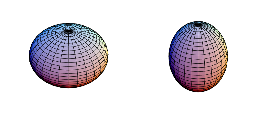
Figure 1: A uniform magnetic field or a cosmic string results in an oblate spheroid shape of the universe (left figure), while domain walls lead to prolate spheroids (right figure) [6].

The energy-momentum tensor of the whole universe can be in general given by

$$T^{\mu}_{\;\;\nu}=\mbox{diag}\,(\rho,-p_{\|},-p_{\|},-p_{\bot}).$$ (4)

Then the Einstein equations read

$$\Bigl{(}\frac{\dot{a}}{a}\Bigr{)}^{2}-\frac{2}{3}\frac{\dot{a}}{a}\frac{e\dot{e}}{1-e^{2}}=\frac{8\pi}{3}G\rho,$$ (5)

$$\Bigl{(}\frac{\dot{a}}{a}\Bigr{)}^{2}+\frac{2\ddot{a}}{a}-3\frac{\dot{a}}{a}\frac{e\dot{e}}{1-e^{2}}-\frac{e\ddot{e}}{1-e^{2}}-\frac{{\dot{e}}^{2}}{(1-e^{2})^{2}}=-8\pi Gp_{\|},$$ (6)

$$\Bigl{(}\frac{\dot{a}}{a}\Bigr{)}^{2}+2\frac{\ddot{a}}{a}=-8\pi Gp_{\bot},$$ (7)

where overdots denote derivatives with respect to the cosmic time. ¿From Eqs. (5), (6) and (7), we get the conservation equation for the energy-momentum tensor

$$\dot{\rho}+2\Bigl{(}\frac{\dot{a}}{a}\Bigr{)}(\rho+p_{\|})+\Bigl{(}\frac{\dot{a}}{a}-2\frac{\dot{e}e}{1-e^{2}}\Bigr{)}(\rho+p_{\bot})=0.$$ (8)

In principle, the total energy-momentum tensor, $T^{\mu}_{~{}\nu}$, can be separated into two different parts: an anisotropic contribution $(T_{A})^{\mu}_{~{}\nu}=diag(\rho^{A},-p^{A}_{\|},-p^{A}_{\|},-p^{A}_{\bot})$, which may include magnetic fields or static aligned strings or static stacked walls, and an isotropic contribution, $({T_{I}})^{\mu}_{~{}\nu}=diag(\rho^{I},-p^{I},-p^{I},-p^{I})$, which includes symmetric contributions from vacuum energy or matter or radiation. As in the isotropic universe, we may have a thermodynamic relation

$$\frac{Tdp^{I}}{dT}=\rho^{I}+p^{I},$$ (9)

where $T$ is the temperature. Up to an additive constant, the entropy in a volume $V$ is given by

$$S=(\rho^{I}+p^{I})\frac{V}{T}.$$ (10)

Using $V\propto\sqrt{1-e^{2}}a^{3}$, we obtain

$$\frac{\dot{S}}{S}=(1-e^{2})^{-\frac{1}{2}}(-2e\dot{e})a^{3}+3a^{2}\dot{a}(1-e^{2})^{\frac{1}{2}}+a^{3}(1-e^{2})^{\frac{1}{2}}\Bigl{(}\frac{\dot{\rho}^{I}}{\rho^{I}+p^{I}}\Bigr{)}.$$ (11)

Assuming an adiabatic expansion of the universe, where the entropy in a comoving volume is conserved, from Eq. (11) we obtain a conservation equation

$$\dot{\rho}^{I}+3\Bigl{(}\frac{\dot{a}}{a}\Bigr{)}(\rho^{I}+p^{I})-\frac{2e\dot{e}}{1-e^{2}}(\rho^{I}+p^{I})=0.$$ (12)

In the limiting case of $e=0$, Eq. (12) is exactly the well-known conservation equation for the energy-momentum tensor in the standard cosmology. For a matter with the equation of state $p^{I}=\omega\rho^{I}$, by solving Eq. (12) we find that the density evolves as

$$\rho^{I}\propto(1-e^{2})^{-(\omega+1)}a^{-3(\omega+1)}.$$ (13)

Therefore, we have $\rho^{I}\propto(1-e^{2})^{-1}a^{-3}$ in the matter-dominant era $(p^{I}=0)$ and $\rho^{I}\propto(1-e^{2})^{-4/3}a^{-4}$ in the radiation-dominant era $(p^{I}=\rho^{I}/3)$. Subtracting Eq. (12) for the isotropic part from the conservation equation (8) for the total energy-momentum, we obtain a similar equation for the anisotropic part

$$\dot{\rho}^{A}+2\Bigl{(}\frac{\dot{a}}{a}\Bigr{)}(\rho^{A}+p^{A}_{\|})+\Bigl{(}\frac{\dot{a}}{a}-\frac{2e\dot{e}}{1-e^{2}}\Bigr{)}(\rho^{A}+p^{A}_{\bot})=0.$$ (14)

Some exact solutions of the Einstein equations for kinds of plane symmetric plus isotropic components are given in Ref. [6].

We now give an example of a uniform magnetic field here, the simplest case, whose physical interpretation in the brane-world scenario will be discussed in Sec. IV. Let us consider the ellipsoidal universe in the matter-dominant era $(p^{I}=0)$, and normalize the scale factors such that $a(t_{0})=c(t_{0})=1$ and thus $e(t_{0})=0$ in the present time. The uniform magnetic field has the energy-momentum tensor ${(T_{A})}^{\mu}_{~{}\nu}=\rho^{A}diag(1,-1,-1,1)$, where $\rho^{A}=B^{2}/8\pi$ is the magnetic energy density. Here, it is assumed that the magnetic field is frozen into the plasma due to the high conductivity of the primordial plasma and the magnetic field evolves as $B\propto a^{-2}$. Then, for a small eccentricity and thus $(1-e^{2})\sim 1$, Eqs. (6), (7) and (14) can be approximately written as

$$\frac{d}{dt}(e\dot{e})+3He\dot{e}=16\pi G\rho^{A},$$ (15)

$$\dot{H}^{2}+2\frac{\ddot{a}}{a}=8\pi G\rho^{A},$$ (16)

$$\dot{\rho}^{A}+4H\rho^{A}=0,$$ (17)

where $H=\dot{a}/a$ is the Hubble constant and $\Lambda$ is the cosmological constant. In the matter-dominant era, we have $a(t)\sim(3H_{0}t/2)^{2/3}$ and then $H=2/3t$. The solution of Eq. (15) is $e^{2}=8\Omega^{A}_{(0)}(1-3a^{-1}+2a^{-3/2})$, where $\Omega^{A}_{(0)}=\rho^{A}(t_{0})/\rho_{\rm cr}^{(0)}$, where $\rho_{\rm cr}^{(0)}=3H_{0}^{2}/8\pi G$ is the actual critical energy density. Since $a(t)<a(t_{0})=1$, the dominant term of the eccentricity is $e^{2}\sim 16\Omega^{A}_{(0)}a^{-3/2}$. The result of Ref. [7] shows that a small eccentricity of order $e_{dec}\sim 10^{-2}$ at the decoupling epoch generated by the uniform cosmic magnetic field with a strength $B_{0}\sim 10^{-9}$G can explain the quadrupole problem without affecting higher multipoles of the angular power spectrum of the temperature anisotropy.

3 Ellipsoidal universe in a bulk

In the following, we discuss the ellipsoidal universe in the brane world cosmology. The main purpose of this section is to derive the corresponding equations governing the evolution of the ellipsoidal universe for the brane metric. In fact, recent results show that brane world cosmological models have the capability to endow dark energy with an excitingly new possibility ($\omega<-1$) without suffering from the problems faced by phantom energy [12]. We consider a 5D spacetime metric with an induced plane-symmetric metric on the brane

$$ds^{2}=\tilde{g}_{AB}dx^{A}dx^{B}=g_{\mu\nu}dx^{\mu}dx^{\nu}-b^{2}dy^{2},$$ (18)

where $y$ is the coordinate in the fifth dimension. Here and hereafter, we focus our attention on the hypersurface defined by $y=0$, which we identify with the world volume of the brane that forms our universe. The upper case Latin letters $A,B,...$ denote 5-dimensional indices, Greek letters $\mu,\nu,...$ denote indices parallel to the brane world volume, 5 an index transverse to the brane, and Latin letters $i,j,...$ denote space-like indices parallel to the brane world volume. We can further take a metric of the form

$$ds^{2} = n^{2}(\tau,y)d\tau^{2}-a^{2}(\tau,y)(dx_{1}^{2}+dx_{2}^{2})-\left(1-e^{2}(\tau,y)\right)a^{2}(\tau,y)dx_{3}^{2}$$ (19)

$$-b^{2}(\tau,y)dy^{2},$$

where the $x_{1}x_{2}$ plane is the plane of symmetry and $n(\tau,y)$ is a lapse function. The five-dimensional Einstein equations take the usual form

$$\tilde{G}_{AB}\equiv\tilde{R}_{AB}-\frac{1}{2}\tilde{R}\tilde{g}_{AB}=\kappa^{2}\tilde{T}_{AB},$$ (20)

where $\tilde{R}_{AB}$ is the five-dimensional Ricci tensor, $\tilde{R}=\tilde{g}^{AB}\tilde{R}_{AB}$ is the scalar curvature, and the constant $\kappa$ is related to the five-dimensional Newton’s constant $G_{(5)}$ and the five-dimensional reduced Planck mass $M_{(5)}$ by the relation, $\kappa^{2}=8\pi G_{(5)}=M^{-3}_{(5)}$. The energy-momentum tensor can be decomposed into two parts

$$\tilde{T}^{A}_{~{}B}=\check{T}^{A}_{~{}B}\mid_{bulk}+{T}^{A}_{~{}B}\mid_{brane},$$ (21)

where $\check{T}^{A}_{~{}B}\mid_{bulk}$ is the energy-momentum tensor of the bulk matter. The bulk tensor $\check{T}^{A}_{~{}B}\mid_{bulk}$ can be further decomposed into two parts: the isotropic contribution, $(\check{T_{I}})^{A}_{~{}B}\mid_{bulk}=\rho^{I}_{B}diag(-1,-1,-1,-1,-1)$, from a cosmological constant, and the anisotropic part, $(\check{T_{\mathcal{A}}})^{A}_{~{}B}\mid_{bulk}=diag(\rho^{\mathcal{A}}_{B},-P^{\mathcal{A}}_{B~{}\|},-P^{\mathcal{A}}_{B~{}\|},-P^{\mathcal{A}}_{B~{}\bot},-P^{\mathcal{A}}_{B~{}T})$, where the bulk energy density and pressures are independent of the coordinate $y$. The second term ${T}^{A}_{~{}B}\mid_{brane}$ corresponds to the matter on the brane($y=0$). The most general energy-momentum tensor consistent with the planar symmetry takes the form

$${T}^{A}_{~{}B}\mid_{brane}=\frac{\delta(y)}{b}diag(\rho,-p_{\|},-p_{\|},-p_{\bot},0).$$ (22)

Substituting Eq. (19) into the Einstein equation, we get the non-vanishing components of the Einstein tensor $\tilde{G}^{A}_{~{}B}$:

$$\tilde{G}^{0}_{I~{}0} = \frac{3}{b^{2}}\Bigl{(}-\frac{a^{\prime 2}}{a^{2}}+\frac{a^{\prime}b^{\prime}}{ab}+\frac{3ea^{\prime}e^{\prime}}{a(1-e^{2})}-\frac{a^{\prime\prime}}{a}\Bigr{)}$$ (23)

$$+3\frac{\dot{a}}{an^{2}}\Bigl{(}\frac{\dot{a}}{a}+\frac{\dot{b}}{b}\Bigr{)}-\frac{e\dot{e}\dot{a}}{an^{2}(1-e^{2})},$$

$$\tilde{G}^{1}_{I~{}1} = G^{2}_{I~{}2}=\frac{1}{b^{2}}\Bigl{(}-\frac{a^{\prime 2}}{a^{2}}+\frac{2a^{\prime}b^{\prime}}{ab}+\frac{2ea^{\prime}e^{\prime}}{a(1-e^{2})}-2\frac{a^{\prime}n^{\prime}}{an}+\frac{b^{\prime}n^{\prime}}{bn}-\frac{2a^{\prime\prime}}{a}-\frac{n^{\prime\prime}}{n}\Bigr{)}$$ (24)

$$+\frac{1}{n^{2}}\Bigl{(}\frac{\dot{a}^{2}}{a^{2}}+\frac{2\dot{a}\dot{b}}{ab}-\frac{2e\dot{a}\dot{e}}{a(1-e^{2})}-2\frac{\dot{a}\dot{n}}{an}-\frac{\dot{b}\dot{n}}{bn}+\frac{2\ddot{a}}{a}+\frac{\ddot{b}}{b}\Bigr{)},$$

$$\tilde{G}^{3}_{I~{}3} = \frac{1}{b^{2}}\Bigl{(}-\frac{a^{\prime 2}}{a^{2}}+\frac{2a^{\prime}b^{\prime}}{ab}-2\frac{a^{\prime}n^{\prime}}{an}+\frac{b^{\prime}n^{\prime}}{nb}-\frac{2a^{\prime\prime}}{a}-\frac{n^{\prime\prime}}{n}\Bigr{)}$$ (25)

$$+\frac{1}{n^{2}}\Bigl{(}\frac{\dot{a}^{2}}{a^{2}}+\frac{2\dot{a}\dot{b}}{ab}-\frac{2\dot{a}\dot{n}}{an}-\frac{\dot{b}\dot{n}}{bn}+\frac{2\ddot{a}}{a}+\frac{\ddot{b}}{b}\Bigr{)},$$

$$\tilde{G}^{0}_{I~{}5} = \frac{1}{n^{2}}\Bigl{(}\frac{3n^{\prime}\dot{a}}{an}+\frac{3a^{\prime}\dot{b}}{ab}-\frac{ea^{\prime}\dot{e}}{a(1-e^{2})}+\frac{3ee^{\prime}\dot{a}}{a(1-e^{2})}-\frac{3\dot{a}^{\prime}}{a}\Bigr{)},$$ (26)

$$\tilde{G}^{5}_{I~{}0} = \frac{1}{b^{2}}\Bigl{(}-\frac{3n^{\prime}\dot{a}}{an}-\frac{3a^{\prime}\dot{b}}{ab}+\frac{ea^{\prime}\dot{e}}{a(1-e^{2})}-\frac{3ee^{\prime}\dot{a}}{a(1-e^{2})}+\frac{3\dot{a}^{\prime}}{a}\Bigr{)},$$ (27)

$$\tilde{G}^{5}_{I~{}5} = \frac{1}{n^{2}}\Bigl{(}\frac{3\dot{a}^{2}}{a^{2}}-\frac{3e\dot{e}\dot{a}}{a(1-e^{2})}-\frac{3\dot{a}\dot{n}}{an}+\frac{3\ddot{a}}{a}\Bigr{)}$$ (28)

$$+\frac{1}{b^{2}}\Bigl{(}-\frac{3a^{\prime 2}}{a^{2}}+\frac{ea^{\prime}e^{\prime}}{a(1-e^{2})}-\frac{3a^{\prime}n^{\prime}}{an}\Bigr{)}.$$

In the above expressions, primes stand for derivatives with respect to $y$, and overdots for derivatives with respect to the cosmic time $\tau$. The reason why we can separate the Einstein tensors into isotropic parts and anisotropic parts is that the corresponding parts of the energy-momentum tensor obey their own conservation equations, Eqs. (12) and (14). We assume that there is no flow of matter along the fifth dimension, i. e. $(\check{T}_{I})_{05}=0$, which in turn implies that $\tilde{G}^{0}_{I~{}5~{}}=\tilde{G}^{5}_{I~{}0}=0$. Then the components $(0,0)$ and $(5,5)$ of Einstein equations (23) and (28) in the bulk can be written in the simple form

$$F^{\prime}=\frac{2a^{\prime}a^{3}}{3}(1-e^{2})\kappa^{2}\check{T}^{0}_{I~{}0},~{}~{}~{}\dot{F}=\frac{2\dot{a}a^{3}}{3}(1-e^{2})\kappa^{2}\check{T}^{5}_{I~{}5},$$ (29)

where $F$ is a function of $\tau$ and $y$ defined by

$$F(\tau,y)=(1-e^{2})\Bigl{[}\Bigl{(}\frac{\dot{a}a}{n}\Bigr{)}^{2}-\Bigl{(}\frac{a^{\prime}a}{b}\Bigr{)}^{2}\Bigr{]}.$$ (30)

Integrating Eq. (30), we obtain the relation

$$\Bigl{(}\frac{\dot{a}}{an}\Bigr{)}^{2}=\Bigl{(}\frac{a^{\prime}}{ab}\Bigr{)}^{2}+\frac{\kappa^{2}}{6}\check{T}^{0}_{I~{}0}-\frac{\int a^{4}d(1-e^{2})}{6a^{4}(1-e^{2})}\check{T}^{0}_{I~{}0}+\frac{\mathcal{C}_{1}}{a^{4}(1-e^{2})},$$ (31)

where $\mathcal{C}_{1}$ is a constant of integration. The above equation shows that the scale factor $a(\tau,y)$ and the eccentricity are coupled to each other. If $e=0$, then Eq. (31) reduces exactly to the result of Ref. [10].

We now consider the anisotropic contribution of the total energy-momentum tensor. The corresponding anisotropic part of the Einstein tensors can be written as

$$\tilde{G}^{0}_{\mathcal{A}~{}0} = \frac{1}{b^{2}(1-e^{2})}\Bigl{(}{ee^{\prime\prime}}+\frac{e^{\prime 2}}{(1-e^{2})}-\frac{eb^{\prime}e^{\prime}}{b}+\frac{ea^{\prime}e^{\prime}}{a}\Bigr{)}$$ (32)

$$-\frac{1}{n^{2}(1-e^{2})}\Bigl{(}\frac{e\dot{a}\dot{e}}{a}+\frac{e\dot{b}\dot{e}}{b}\Bigr{)},$$

$$\tilde{G}^{1}_{\mathcal{A}~{}1} = \tilde{G}^{2}_{\mathcal{A}~{}2}=\frac{1}{b^{2}(1-e^{2})}\Bigl{(}\frac{ea^{\prime}e^{\prime}}{a}-\frac{eb^{\prime}e^{\prime}}{b}+\frac{e^{\prime 2}}{(1-e^{2})}+ee^{\prime}n^{\prime}+{ee^{\prime\prime}}\Bigr{)}$$ (33)

$$-\frac{1}{n^{2}(1-e^{2})}\Bigl{(}\frac{e\dot{a}\dot{e}}{b}+\frac{e\dot{b}\dot{e}}{b}+\frac{\dot{e}^{2}}{(1-e^{2})}-\frac{e\dot{e}\dot{n}}{n}+\ddot{e}e\Biggr{)},$$

$$\tilde{G}^{3}_{\mathcal{A}~{}3} = 0,$$ (34)

$$\tilde{G}^{0}_{\mathcal{A}~{}5} = \frac{1}{n^{2}(1-e^{2})}\Bigl{(}-\frac{ee^{\prime}\dot{a}}{a}-\frac{ee^{\prime}\dot{b}}{b}+\frac{ea^{\prime}\dot{a}}{a}+\frac{e^{\prime}\dot{e}}{(1-e^{2})}-\frac{en^{\prime}\dot{e}}{n}+e\dot{e}^{\prime}\Bigr{)},$$ (35)

$$\tilde{G}^{5}_{\mathcal{A}~{}0} = \frac{1}{b^{2}(1-e^{2})}\Bigl{(}\frac{ee^{\prime}\dot{a}}{a}+\frac{ee^{\prime}\dot{b}}{b}-\frac{ea^{\prime}\dot{a}}{a}-\frac{e^{\prime}\dot{e}}{(1-e^{2})}+\frac{en^{\prime}\dot{e}}{n}-{e\dot{e}^{\prime}}\Bigr{)},$$ (36)

$$\tilde{G}^{5}_{\mathcal{A}~{}5} = \frac{1}{1-e^{2}}\Bigl{(}\frac{ea^{\prime}e^{\prime}}{ab^{2}}+\frac{ee^{\prime}n^{\prime}}{b^{2}}-\frac{e\dot{a}\dot{e}}{an^{2}}-\frac{\dot{e}^{2}}{n^{2}}+\frac{e\dot{e}\dot{n}}{n^{3}}-\frac{e\ddot{e}}{n^{2}}\Bigr{)}.$$ (37)

Here we also assume that $\check{T}^{0}_{\mathcal{A}~{}5}=0$, that is to say no flow of anisotropic matter (magnetic fields or cosmic strings or domain walls) along the fifth dimension and so $G^{0}_{\mathcal{A}~{}5}=G^{5}_{\mathcal{A}~{}0}=0$. Eqs. (32) and (37) can be written as

$$K^{\prime}\simeq 2ee^{\prime}(1-e^{2})a^{2}\kappa^{2}\check{T}^{0}_{\mathcal{A}~{}0},~{}~{}~{}\dot{K}\simeq 2e\dot{e}(1-e^{2})a^{2}\kappa^{2}\check{T}^{5}_{\mathcal{A}~{}5},$$ (38)

where $K$ is defined by

$$K=\Bigl{(}\frac{aee^{\prime}}{b}\Bigr{)}^{2}-\Bigl{(}\frac{ae\dot{e}}{n}\Bigr{)}^{2}.$$ (39)

Integrating Eq. (38) we obtain

$$\Bigl{(}\frac{e\dot{e}}{(1-e^{2})n}\Bigr{)}^{2}=\Bigl{(}\frac{ee^{\prime}}{(1-e^{2})b}\Bigr{)}^{2}+\frac{1}{2}\kappa^{2}\check{T}^{0}_{\mathcal{A}~{}0}+\frac{\int(1-e^{2})da^{2}}{a^{2}(1-e^{2})}\check{T}^{0}_{\mathcal{A}~{}0}+\frac{\mathcal{C}_{2}}{a^{2}(1-e^{2})^{2}},$$ (40)

where $\mathcal{C}_{2}$ is another integration constant.

We now take the brane into consideration by using the Israel’s junction condition [13]. When the coordinate system (18) is chosen, the extrinsic curvature tensor of a given hypersurface (for example, the $y=0$ surface) is defined by $K_{\mu\nu}=\partial_{y}g_{\mu\nu}/2$. The Israel’s junction condition at $y=0$ can be written as [14, 15]

$$\{K_{\mu\nu}-Kg_{\mu\nu}\}_{y}=-\frac{\kappa^{2}}{2}T_{\mu\nu},$$ (41)

where $K$ is defined by $K\equiv K_{\mu\nu}g^{\mu\nu}$, $T_{\mu\nu}$ is the energy-momentum tensor of the brane. We have assumed a brane with $Z_{2}$ symmetry and the index _y means accordingly that the value of the component $K_{\mu\nu}$ is taken over one side of the brane, namely at $y=0^{+}$. The junction condition on the planar symmetric metric background are given by

$$\frac{[a^{\prime}]}{a_{0}b_{0}} = \frac{\kappa^{2}}{3}\rho+\frac{\kappa^{2}}{3}(p_{\|}-p_{\bot}),$$ (42)

$$\frac{e_{0}[e^{\prime}]}{b_{0}(1-e_{0}^{2})} = \kappa^{2}(p_{\|}-p_{\bot}),$$ (43)

$$\frac{[n^{\prime}]}{n_{0}b_{0}} = -\frac{\kappa^{2}}{3}(2\rho+2p_{\|}+p_{\bot})$$ (44)

where the subscript $0$ for $a$, $b$, and $n$ means that they are taken at $y=0$, and $[Q]=Q(0^{+})-Q(0^{-})$ denotes the jump of the function $Q$ across $y=0$. From Eqs. (42)-(44), we can see that when $p_{\|}=p_{\bot}$ the boundary conditions reduce to the spherical cases discussed in Ref. [10]. Assuming the symmetry $y\leftrightarrow-y$ for simplicity, the junction conditions (42)-(44) can be used to compute $a^{\prime}$ and $e^{\prime}$ on the two sides of the brane, and by continuity when $y\rightarrow-y$, Eq. (31) and Eq. (40) are reexpressed as (after setting $n_{0}=1$)

$$\Bigl{(}\frac{\dot{a}}{a_{0}}\Bigr{)}^{2}=\frac{\kappa^{2}\rho_{B}^{I}}{6}+\frac{\kappa^{4}\rho^{2}}{36}+\frac{\kappa^{4}}{36}(p_{\|}-p_{\bot})^{2}-\frac{\int a^{4}d(1-e^{2})}{6a_{0}^{4}(1-e_{0}^{2})}\rho_{B}^{I}+\frac{\mathcal{C}_{1}}{a_{0}^{4}(1-e_{0}^{2})}~{}~{}$$ (45)

$$\Bigl{(}\frac{{e_{0}}{\dot{e}}_{0}}{1-{e_{0}}^{2}}\Bigr{)}^{2}=\frac{\kappa^{4}}{4}(p_{\|}-p_{\bot})^{2}+\frac{\kappa^{2}}{2}\rho_{B}^{\mathcal{A}}+\frac{\int(1-e^{2})da^{2}}{a_{0}^{2}(1-e_{0}^{2})^{2}}\rho_{B}^{\mathcal{A}}+\frac{\mathcal{C}_{2}}{a_{0}^{2}(1-e_{0}^{2})^{2}}.$$ (46)

The above two equations are the main results of our work. From Eq. (45), we can see that when $p_{\|}=p_{\bot}$, the scale factor is exactly what was found in Ref. [10]. If the third term in Eq. (45) is small compared with the other terms, it play a role of perturbation and the Friedman equation does not deviate much from that of Ref. [10]. Eq. (46) describes the evolution of the eccentricity on the brane world, which shows that the evolution of the eccentricity depends on both the brane anisotropic pressures and the bulk anisotropic energy density. We should notice that the energy conservation on the brane, which was obtained in Sec. II, still works here

$$\dot{\rho}+2\Bigl{(}\frac{\dot{a}}{a}\Bigr{)}(\rho+p_{\|})+\Bigl{(}\frac{\dot{a}}{a}-2\frac{\dot{e}e}{1-e^{2}}\Bigr{)}(\rho+p_{\bot})=0.$$ (47)

Since the scale factor and the eccentricity are coupled to each other, we do not expect to solve Eqs. (45) and (46) exactly. But for a small eccentricity, i.e. $\rho\sim(1-e^{2})^{-(\omega+1)}a^{-3(\omega+1)}\approx a^{-3(\omega+1)}$ and when the third term in Eq. (45) can be neglected, the time evolution of the scale factor can be given by [10]

$$a_{0}(t)=a_{*}(\kappa^{2}\rho_{*})^{1/q}\Bigl{(}\frac{q^{2}}{72}\kappa^{2}\rho_{\Lambda}t^{2}+\frac{q}{6}t\Bigr{)}^{1/q},$$ (48)

where the energy density on the brane has been decomposed into three parts $\rho=\rho^{I}+\rho^{\mathcal{A}}+\rho_{\Lambda}$, $q=3(\omega+1)$, $a_{*}$ and $\rho_{*}$ are constants, and $\rho_{\Lambda}$ is a constant that represents an intrinsic tension of the brane. Here the Randall-Sundrum relation, $\kappa^{2}\rho_{B}^{I}/6+\kappa^{2}\rho_{\Lambda}^{2}/36=0$ has been used [16]. Eq. (48) indicates that at a very early universe, the cosmology is characterized by $a(t)\sim t^{1/q}$, while at a late time it is described by the standard cosmology, $a\sim t^{2/q}$. We are going to solve Eq. (46), by considering only the first term and neglecting others. We still assume the anisotropy of the our universe is contributed by a uniform magnetic field with the energy-momentum tensor ${(T_{\mathcal{A}})}^{\mu}_{~{}\nu}=\rho^{{\mathcal{A}}}diag(1,-1,-1,1)$, and thus from Eq. (47) we find that $\rho^{{\mathcal{A}}}\propto a^{-4}$. Substituting $a\sim t^{1/q}$ , $H=1/qt$, and $\rho^{{\mathcal{A}}}=\rho_{0}^{{\mathcal{A}}}a^{-4}$ back to Eq. (46), we obtain

$$e^{2}=\frac{2\kappa^{2}\rho_{0}^{{\mathcal{A}}}t^{1-\frac{4}{q}}}{q-4}+\mathcal{C}_{3},$$ (49)

where $\mathcal{C}_{3}$ is an integration constant. Similarly, at a late time of the universe, $a\sim t^{2/q}$ , $H=2/qt$, and $\rho^{A}=\rho_{0}^{{\mathcal{A}}}a^{-4}$, the eccentricity is expressed as

$$e^{2}=\frac{2\kappa^{2}\rho_{0}^{{\mathcal{A}}}t^{1-\frac{8}{q}}}{q-8}+\mathcal{C}_{4},$$ (50)

where $\mathcal{C}_{4}$ is also another integration constant. In the matter-dominant era $(q=3)$, we find that the late-time evolution of eccentricity in the bulk approximately is $e^{2}\sim a^{-5/2}$, which decays a little faster than that in 4D universe, while $e^{2}\sim a^{-1}$ for a very early universe $a\sim t^{1/q}$ with $q=3$.

4 Ellipsoidal Universe in the brane-induced gravity model

In this section, we explore a scenario of the ellipsoidal universe based on the Dvali-Gabadadze-Porrati (DGP) model of brane-induced gravity [17]. In this model, the 3-brane is embedded in a spacetime with an infinite-size extra dimension. The usual gravitational laws is obtained by adding to the action of the brane an Einstein-Hilbert term computed with the intrinsic curvature on the brane. Particularly, one recovers a standard four-dimensional (4D) Newtonian potential for small distances, whereas gravity is in a 5D regime for large distances. The cosmology of this model in the case of a 5D bulk was studied by Daffayet, Dvali and Gabadadze. It is shown there that if the cosmological model contains a scalar curvature term in the action for the brane, besides the brane and bulk cosmological constraints, the presence of the scalar curvature term in the brane action can lead to a late-time acceleration of the universe even in the absence of any material form of dark energy [8, 9].

Following the framework of Refs. [8, 9], we consider a 3-brane embedded in a 5D spacetime with an intrinsic curvature term induced on the brane and the action of the form

$$S_{(5)}=-\frac{1}{2\kappa^{2}}\int d^{5}x\sqrt{-\tilde{g}}\tilde{R}+\int d^{5}x\mathcal{L}_{m}-\frac{1}{2\mu^{2}}\int d^{4}x\sqrt{-g}R$$ (51)

The first term in Eq. (51) corresponds to the Einstein-Hilbert action in five dimensions for a 5D metric $\tilde{g}_{AB}$(bulk metric). Similarly, the last term in (51) is the Einstein-Hilbert action for the induced metric $g_{cd}$ on the brane, $R$ being its scalar curvature. The induced metric $g_{cd}$ is defined as usual from the bulk metric, $g_{cd}=\partial_{c}X^{A}\partial_{d}X^{B}\tilde{g}_{AB}$, where $X^{A}(x^{c})$ represents the coordinates of an event on the brane labeled by $x^{c}$. The second term in (51) denotes the matter content.

The five-dimensional Einstein equations in the brane-induced gravity is given by

$$\tilde{G}_{AB}\equiv\tilde{R}_{AB}-\frac{1}{2}\tilde{R}\tilde{g}_{AB}=\kappa^{2}\tilde{S}_{AB},$$ (52)

where the tensor $\tilde{S}$ is the sum of the energy-momentum tensor $\tilde{T}$ of matter and the contribution coming from the scalar curvature of the brane. We denote the latter contribution $\tilde{U}$, so

$$\tilde{S}^{A}_{~{}B}=\tilde{T}^{A}_{~{}B}+\tilde{U}^{A}_{~{}B}.$$ (53)

The junction condition in the brane-induced gravity model is replaced by $\{K_{\mu\nu}-Kg_{\mu\nu}\}_{q}=-(\kappa^{2}/2)S_{\mu\nu},$ with $S_{\mu\nu}=T_{\mu\nu}-(1/\mu^{2})U_{\mu\nu}$, where $\mu^{2}$ is the four-dimensional Newton’s constant, $\mu^{2}=8\pi G_{(4)}=M_{(4)}^{-2}$. The Israel boundary condition is then written as

$$\frac{[a^{\prime}]}{a_{0}b_{0}} = \frac{\kappa^{2}}{3}\rho+\frac{\kappa^{2}}{3}(p_{\|}+p_{\bot})-\frac{\kappa^{2}}{3\mu^{2}n^{2}_{0}}$$ (54)

$$\Bigl{(}3\frac{\dot{a}^{2}}{a^{2}_{0}}+\frac{e_{0}\dot{a}\dot{e}}{a_{0}(1-e^{2}_{0})}+\frac{e_{0}\ddot{e}}{1-e^{2}_{0}}-\frac{e_{0}\dot{e}\dot{n}}{n_{0}(1-e^{2}_{0})}+\frac{\dot{e}^{2}}{(1-e^{2}_{0})^{2}}\Bigr{)},$$

$$\frac{e_{0}[e^{\prime}]}{b_{0}(1-e^{2}_{0})} = \kappa^{2}(p_{\|}-p_{\bot})$$ (55)

$$- \frac{\kappa^{2}}{\mu^{2}n^{2}_{0}}\Bigl{(}\frac{3e_{0}\dot{a}\dot{e}}{a_{0}(1-e^{2}_{0})}+\frac{e_{0}\ddot{e}}{1-e^{2}_{0}}-\frac{e_{0}\dot{e}\dot{n}}{n_{0}(1-e^{2}_{0})}+\frac{\dot{e}^{2}}{(1-e^{2}_{0})^{2}}\Bigr{)},$$

$$\frac{[n^{\prime}]}{n_{0}b_{0}} = -\frac{\kappa^{2}}{3}(2\rho+2p_{\|}+p_{\bot})+\frac{\kappa^{2}}{\mu^{2}n^{2}_{0}}\Bigl{(}\frac{\dot{a}^{2}}{a^{2}_{0}}+2\frac{\dot{a}\dot{n}}{a_{0}n_{0}}-\frac{2\ddot{a}}{a_{0}}\Bigr{)}+\frac{2\kappa^{2}}{3\mu^{2}n^{2}_{0}}$$ (56)

$$\Bigl{(}\frac{e_{0}\dot{a}\dot{e}}{a_{0}(1-e^{2}_{0})}+\frac{e_{0}\ddot{e}}{1-e^{2}_{0}}-\frac{e_{0}\dot{e}\dot{n}}{n_{0}(1-e^{2}_{0})}+\frac{\dot{e}^{2}}{(1-e^{2}_{0})^{2}}\Bigr{)}~{}.~{}$$

Substituting Eqs. (31), (40), (54) and (55) into the (0,0)-component of the Israel’s junction condition and assuming $\rho_{B}^{I}$, $\rho_{B}^{\mathcal{A}}$, $\mathcal{C}_{1}$ and $\mathcal{C}_{2}$ to be approximately zero, we have

$$\Bigl{(}H-\epsilon\frac{\mu^{2}}{\kappa^{2}}\Bigr{)}^{2}-\frac{2}{3}\frac{e\dot{e}}{1-e^{2}}\Bigl{(}H-\epsilon\frac{\mu^{2}}{\kappa^{2}}\Bigr{)}\simeq\frac{\mu^{2}}{3}\rho+\epsilon^{2}\frac{\mu^{4}}{\kappa^{4}},$$ (57)

where $H=\dot{a}/a_{0}$, $\epsilon$ is the sign of $[a^{\prime}]$ such that $\epsilon=\pm 1$ and the lapse function is set to be $n_{0}=1$. One should note that when $\mu^{2}/\kappa^{2}<2\mu^{2}/\kappa^{2}\ll H$, or in terms of the Hubble radius $H^{-1}$, when $H^{-1}\ll M_{(4)}^{2}/2M_{(5)}^{3}$, the 4D ellipsoidal universe is recovered, i.e. one can return to Eq. (5).

We notice that from Eqs. (40) and (55) with vanishing anisotropic bulk energy-momentum tensor $\rho_{B}^{\mathcal{A}}$ and vanishing $\mathcal{C}_{2}$, it follows that

$$\Bigl{(}\frac{e\ddot{e}}{1-e^{2}}+\frac{\dot{e}^{2}}{(1-e^{2})^{2}}\Bigr{)}+{\frac{(e\dot{e})}{(1-e^{2})}}\Bigl{(}3\frac{\dot{a}}{a}+2\epsilon\frac{\mu^{2}}{\kappa^{2}}\Bigr{)}={\mu^{2}}(p_{\|}-p_{\bot}).$$ (58)

When $2\epsilon\mu^{2}/\kappa^{2}$ in the second term can be neglected, then Eq. (58) exactly equals to Eq. (7) subtracted by Eq. (6). In the small eccentricity approximation $1-e^{2}\sim 1$, we solve Eq. (58) in the matter-dominant era with $a\sim t^{2/3}$ and $H=2/3t$. We normalize the scale factor such that $a(t_{0})=1$ and $e(t_{0})=0$ in the present time and consider the anisotropy on the brane contributed by a uniform magnetic field with the energy-momentum tensor ${(T_{{\mathcal{A}}})}^{\mu}_{~{}\nu}=\rho^{{\mathcal{A}}}diag(1,-1,-1,1)$. The solution of Eq. (58) can be approximately written as

$$e^{2}(t) \sim \int_{t}^{t_{0}}4\pi\rho_{0}^{A}e^{-2\epsilon\frac{\mu^{2}}{\kappa^{2}}t^{\prime}}t^{\prime-2}dt^{\prime}$$ (59)

$$= \int_{t}^{t_{0}}4\pi\rho_{0}^{A}\Bigl{(}1-2\epsilon\frac{\mu^{2}}{\kappa^{2}}t^{\prime}+\frac{4\frac{\mu^{4}}{\kappa^{4}}t^{\prime 2}}{2!}+\cdots\Bigr{)}t^{\prime-2}dt^{\prime}.$$

Eq. (59) indicates that $\epsilon$ should be $1$, otherwise the eccentricity in the brane does not converge when $t\rightarrow\infty$. Fortunately, Ref. [8] shows that the brane cosmology with $\epsilon=1$ can produce a late-time accelerated expansion. When $2\mu^{2}/\kappa^{2}\ll H$ and then $e^{-2\epsilon\frac{\mu^{2}}{\kappa^{2}}t}\simeq e^{-2\epsilon\frac{\mu^{2}}{\kappa^{2}}H^{-1}}\sim 1$, thus $e^{2}(t)\sim t^{-1}\sim a^{-3/2}$, which is exactly the dominant term of the 4D case. Integrating Eq. (59), the eccentricity on the brane can be written as

$$e^{2}(t)\simeq\frac{1}{3}\Omega^{\mathcal{A}}_{(0)}\Bigl{(}a^{-3/2}+2\frac{\ln a}{r_{c}}-\frac{a^{3/2}}{r_{c}^{2}}\Bigr{)},$$ (60)

where $\Omega^{\mathcal{A}}_{(0)}=\rho^{\mathcal{A}}(t_{0})/\rho_{\rm cr}^{(0)}$, $\rho_{\rm cr}^{(0)}=3H_{0}^{2}/8\pi G$ and $r_{c}=\kappa^{2}/2\mu^{2}=M_{(4)}^{2}/2M_{(5)}^{3}$ is the length scale for the crossover between 4D gravity and the 5D gravity regimes [17]. Differently from that of the 4D case, the brane-induced gravity contributes some higher order corrections to the eccentricity duo to the presence of an extra dimension.

5 Discussion and Conclusion

In the brane cosmology we have found the Friedmann-like equation for the ellipsoidal universe in the bulk, which depends on the geometry and matter (both isotropic and anisotropic) content of the brane. We also have found that the evolution equation of the eccentricity in the bulk depends only on the anisotropic pressures inside the brane and the anisotropic energy density in the bulk, except a constant parameter. The evolution equation of the eccentricity is coupled to that of the scale factor. As a model calculation, we have shown that if only a uniform magnetic field inside the brane contributes to the anisotropy of our universe but the anisotropic energy density from the bulk and other terms are neglected, the evolution of the eccentricity decays faster than that in a 4D universe. To compare with the 4D ellipsoidal universe, we have considered the ellipsoidal universe with a 3-brane embedded in a 5D spacetime with an intrinsic curvature term included in the brane action. The results show that the usual ellipsoidal cosmology is recovered for Hubble radii smaller than the crossover scale given by $r_{c}={M_{(4)}^{2}}/{2M_{(5)}^{3}}$ between 4D and 5D gravity.

We now briefly discuss the relation between eccentricity and cosmic microwave background quadrupole problem. For a small eccentricity of the universe in the brane, the metric tensor may be written in a perturbation form

$$ds^{2}=dt^{2}-a^{2}(t,y)(\delta_{ij}-h_{ij})dx^{i}dx^{j}-b^{2}(t,y)dy^{2},$$ (61)

where $h_{ij}$ represents a metric perturbation, $h_{ij}=e^{2}\delta_{i3}\delta_{j3}$. Suppose a photon emitted at $t=t_{dec}$ from the last scattering surface travels along a null geodesic and reaches an observer at $t=t_{0}$. Let $n^{i}$ be a unit vector along the null ray from the observer to the surface. With respect to the observer at the origin, the photon ray is $x^{i}(t)=\eta(t)n^{i}$, where $\eta(t)=\int_{t}^{t_{0}}dt^{\prime}/a(t^{\prime})$. The geodesic deviation between an observer at $x^{i}$ and another observer at $x^{i}+\delta x^{i}$ along the ray at any time $t$ is given by $\delta l=(-g_{ij}\delta x^{i}\delta x^{j})\propto a(1-h_{ij}n^{i}n^{j}/2)$ to first order in $h_{ij}$. ¿From the proper velocity $v=d\delta l/dt$ of one observer with respect to another and the redshift of the photon’s physical frequency $\delta\omega_{p}/\omega_{p}=-v$, we find the redshift of the comoving frequency

$$\frac{\delta\omega_{c}}{\omega_{c}}=\frac{\delta(\omega_{p}a)}{\omega_{p}a}=\frac{1}{2}\frac{\partial h_{ij}}{\partial t}n^{i}n^{j}\delta t.$$ (62)

As the temperature of radiation with respect to the comoving observer is proportional to the frequency $(\delta T\propto\omega_{c})$, we may find the temperature variation from Eq. (62) as

$$\frac{\delta T}{T_{0}}=\frac{1}{2}\int_{t_{dec}}^{t_{0}}\frac{\partial h_{ij}}{\partial t}n^{i}n^{j}dt=\frac{1}{2}e^{2}_{\rm dec}n^{2}_{3},$$ (63)

where $n_{\rm 3}(\theta,\phi)=\cos\theta\cos\vartheta-\sin\theta\sin\vartheta\cos(\phi-\varphi)$ and $\vartheta,\varphi$ are the angles between spherical galactic coordinates and the c-axis and a-axis respectively [7].

On the other hand, the relative temperature anisotropy $\delta T(\theta,\phi)/T_{0}$ leads to the power spectrum

$$\frac{\delta T_{l}}{\langle T\rangle}=\sqrt{\frac{1}{2\pi}\,\frac{l(l+1)}{2l+1}\sum_{m}|a_{lm}|^{2}},$$ (64)

where $a_{lm}$ is the coefficient of spherical harmonics $Y_{lm}(\theta,\phi)$ and $\langle T\rangle=2.726\pm 0.010K$ is the actual average temperature of the CMB radiation. The power spectrum (64) fully describes all the CMB anisotropy and $l=2$ refers to the quadrupole anisotropy. Recent WMAP data hints a violation of statistical isotropy on its largest scales and a missing power at scales greater than $60^{\circ}$ [1]. Particularly, the observed quadrupole anisotropy

$$(\delta T_{2})^{2}_{obs}\simeq 236\mu K^{2},$$ (65)

deviates by order of magnitude from the prediction of standard inflation

$$(\delta T_{2})^{2}_{I}\simeq 1252\mu K^{2}.$$ (66)

This anomaly is called the quadrupole problem. Since we have assumed that the large-scale spatial geometry of our universe on the brane is plane symmetric with a small eccentricity, the observed CMB anisotropy map is a linear superposition of two independent contributions $\delta T=\delta T_{A}+\delta T_{I}$, where $\delta T_{A}$ represents the temperature fluctuations due to the anisotropic spacetime background, while $\delta T_{I}$ is the standard isotropic fluctuation caused by the inflation-led gravitational potential at the last scattering surface. Similarly, we may write $a_{lm}=a^{A}_{lm}+a^{I}_{lm}$, where $a^{A}_{lm}=(1/2)\int_{0}^{2\pi}\int_{0}^{\pi}e^{2}_{\rm dec}n^{2}_{3}Y^{*}_{lm}sin\theta d\theta d\phi$. Finally we note that while the quadrupole anisotropy contributed by the uniform magnetic field is $\mathcal{S}_{A}=\delta T_{2}/\langle T\rangle=(2/5\sqrt{3})e^{2}_{\rm dec}$ with an eccentricity of order $10^{-2}$, the predicted quadrupole anisotropy can be in a range of $46.2\mu\mbox{K}^{2}\leq\left(\delta T_{2}\right)^{2}\leq 1001.6\,\mu\mbox{K}^{2}$ (for detailed calculations, see Ref. [7]). Thus the data is in agreement with observations.

The equation that governs the evolution of eccentricity in a five-dimensional bulk is found in Sec. III, which is shown to depend on the anisotropic pressures inside the brane and the anisotropic energy density in the bulk. If anisotropy of the our universe is contributed by a uniform magnetic field inside the brane, and neglecting the anisotropic energy density from the bulk and other terms, the evolution of the eccentricity decays faster than that in a 4D ellipsoidal universe. Since the evolution of eccentricity here is described by a 5-dimensional Newton’s constant and is inconvenient to be compared with observational data, we have come to focus on the case of ellipsoidal universe in the brane-induced gravity in Sec. IV. The perturbational metric takes the form of Eq. (61) where we have assumed the fifth dimension to be stabilized under the perturbation. This is because the origin of eccentricity is contributed by the magnetic field which according to Ho$\rm{\check{r}}$ava-Witten picture is confined to a 3-brane [18]. From Eq. (60), we can determine the value of $e^{2}_{\rm dec}$. At the decoupling, $t=t_{\rm dec}$, we have $e^{2}_{\rm dec}\simeq\frac{1}{3}\Omega^{\mathcal{A}}_{(0)}(z^{3/2}_{\rm dec}-2\frac{\rm{ln}z_{\rm dec}}{r_{c}}-\frac{z^{-3/2}_{\rm dec}}{r^{2}_{c}})$, where $z_{\rm dec}\simeq 1088$ is the redshift at decoupling [19]. For large $r_{c}$ (for example, $r_{c}=1.21^{+0.09}_{-0.09}H^{-1}_{0}$ [8]), we have $e^{2}_{\rm dec}\simeq\frac{1}{3}\Omega^{\mathcal{A}}_{(0)}z^{3/2}_{\rm dec}$. Finally, we get $e_{\rm dec}\simeq\frac{1}{4\sqrt{3}}10^{-2}h^{-1}\frac{B_{0}}{10^{-8}G}$, where $B_{0}=B(t_{0})$ is defined by $\rho^{{\mathcal{A}}}_{0}=B^{2}_{0}/8\pi$, and $h\simeq 0.72$. Thus, for $B_{0}\simeq(4-5)\times 10^{-9}$G, we have $e_{\rm dec}\simeq(0.1-0.2)\times 10^{-2}$. Therefore, in the brane-induced gravity model, the evolution of eccentricity in the brane can also be used to explain the quadrupole problem of the cosmic microwave background.

In summary, we have considered a version of ellipsoidal universe in the brane world scenario. Here, we emphasize that the ellipsoidal universe discussed above is undergoing a homogenous but anisotropic expansion. That is to say, before the onset of inflation, a typical region of the universe is homogeneous and isotropic but in some regions an asymmetric expansion driven by magnetic fields would have stretched out the regions and left with an imprint through the end of inflation [6]. The ellipsoidal universe has been used to explain the suppression of quadrupole moment, but not all the low multipoles since in the ellipsoidal coordinate all the coefficients $a^{A}_{lm}$ with $l>2$ vanish. This can be easily found by calculating the formula $a^{A}_{lm}=(1/2)\int_{0}^{2\pi}\int_{0}^{\pi}e^{2}_{\rm dec}n^{2}_{3}Y^{*}_{lm}sin\theta d\theta d\phi$. In the above discussions, we have also investigated the ellipsoidal universe in the DGP model and used a large $r_{c}$ in obtaining the value of eccentricity. We notice that up to now the comparison between data and the DGP model based upon the expansion history of the universe is still contradictory. Recent data of Supernova and CMB suggested that the self-accelerating branch of the DGP model is somehow disfavored [20, 21, 22, 23, 24, 25, 26], while the most recent analysis of the new ’gold’ data set of supernovae [27] and the CMB shift parameter suggested that a flat universe is completely consistent with the DGP model [28, 29]. However, as the density perturbations of the DGP model may differ from those of $\Lambda$CDM model, it is still unclear at present whether the DGP model is marginally or significantly disfavored or not [30, 31, 32]. A full examination of this issue is beyond the scope of this paper, but from Eq. (60) we can see that a large enough $r_{c}$ contributes little to the value of the eccentricity.

References

References

[1] Hinshaw G et al, 2006 Preprint [astro-ph/0603451]
[2] Collins C B, Hawking S W, 1973
Mon. Not. Roy. Astron. Soc.162 307 ;
Barrow J D, Juszkiewicz R and Sonoda D H,
1985
Mon. Not. Roy. Astron. Soc.213 917
[3] Bunn E F, Ferreira P and Silk J, 1996
Phys. Rev. Lett.77 2883
[4] Cornish N Jet al, 2004
Phys. Rev. Lett.92 201302 ;
Roukema B Fet al, 2004
Astron. Astrophys.423 821 ;
Jaffe T R et al, 2005
Astrophys. J.629 L1
[astro-ph/0606046];
Cresswell J G et al, 2006
Phys. Rev. D73 041302;
Ghosh T, Hajian A and Souradeep T, 2006 Preprint [astro-ph/0604279]
[5] Tegmark M, de Oliveira-Costa A and Hamilton A, 2003 Phys. Rev. D68 123523;
de Oliveira-Costa A, Tegmark M,
Zaldarriage M and Hamilton A, 2004 Phys. Rev. D69 063516;
Copi C J, Huterer D and Starkman G D, 2003
Preprint [astro-ph/0310511]
[6] Berera A, Buniy R V and Kephart T W, 2004
J. Cosmol. Astropart. Phys.
JCAP 016(2004) 0410;
Buniy R V, Berera A and Kephart T W, 2006
Phys. Rev. D73 063529
[7] Campanelli L, Cea P and Tedesco L, 2006
Phys. Rev. Lett.97 131302
[8] Deffayet C, Dvali G and Gabadadze G, 2002 Phys. Rev. D65 044023;
Deffayet C, Landau S J, Raux J, Zaldarriaga M
and Astier P, 2002 Phys. Rev. D 66 024019 [astro-ph/0201164]
[9] Deffayet C, 2001 Phys. Lett. B502 199
[10] Bintruy P,Deffayet C, Ellwanger U and Langlois
D, 2000
Phys. Lett. B477 285 [
hep-th/9910219]
[11] Taub A H, 1951 Annals Math. 53 472
[12] Sahni V and Shtanov Y, 2003 J. Cosmol. Astropart. Phys. JCAP014
0311;
R.G. Cai, Y. Gong and B. Wang, 2006 J. Cosmol. Astropart. Phys. JCAP006
0603 [hep-th/0511301]