Spontaneous Breaking of Classical $\mathcal{P}\mathcal{T}$ Symmetry

Abstract

The classical trajectories of the family of complex $\mathcal{P}\mathcal{T}$-symmetric Hamiltonians $H=p^{2}+x^{2}(ix)^{\epsilon}$ ($\epsilon\geq 0$) form closed orbits. All such complex orbits that have been studied in the past are $\mathcal{P}\mathcal{T}$ symmetric (left-right symmetric). The periods of these orbits exhibit an unusual dependence on the parameter $\epsilon$. There are regions in $\epsilon$ of smooth behavior interspersed with regions of rapid variation. It is demonstrated that the onset of rapid variation is associated with strange new kinds of classical trajectories that have never been seen previously. These rare kinds of trajectories are not $\mathcal{P}\mathcal{T}$ symmetric and occur only for special rational values of $\epsilon$.

I Introduction

The classical trajectories $x(t)$ of the family of complex $\mathcal{P}\mathcal{T}$-symmetric Hamiltonians

$$H=p^{2}+x^{2}(ix)^{\epsilon}\qquad(\epsilon\geq 0)$$ (1)

have been examined in detail r1 . One can plot graphs of these trajectories by solving numerically the system of Hamilton’s differential equations dargweb

$${\dot{x}}=\frac{\partial H}{\partial p}=2p,\quad{\dot{p}}=-\frac{\partial H}{\partial x}=-(2+\epsilon)x(ix)^{\epsilon}$$ (2)

for a given set of initial conditions $x(0)$, $p(0)$. Since $x(0)$ and $p(0)$ are not necessarily real numbers and the differential equations (2) are complex, the classical trajectories are curves in the complex-$x$ plane. It is known r1 that for $\epsilon\geq 0$ nearly all trajectories are closed curves. (When $\epsilon$ is a positive integer, it is possible for trajectories that originate at some of the turning points to run off to infinity. However, we are not interested here in these isolated singular cases. When $\epsilon<0$, all trajectories are open curves.) If $\epsilon$ is noninteger, there is a branch cut in the complex-$x$ plane, and we take this cut to run from $0$ to $\infty$ along the positive-imaginary axis. Thus, it is possible for a closed classical trajectory to visit many sheets of the Riemann surface before returning to its starting point.

The non-Hermitian Hamiltonians (1) are remarkable because when they are quantized, their spectra are entirely real and positive r2 ; r3 . Moreover, these Hamiltonians specify a unitary time evolution r4 of the vectors in the associated Hilbert space. Thus, it is important to understand the nature of the complex classical systems underlying these quantum systems.

Several studies r5 ; r6 of the classical trajectories $x(t)$ of complex Hamiltonians were done prior to the work in Ref. r1 and from all these studies many features of the complex trajectories of $\mathcal{P}\mathcal{T}$-symmetric Hamiltonians (1) are known. However, some of the conclusions of the earlier work are wrong. For example, when $\epsilon\geq 0$, the $\mathcal{P}\mathcal{T}$ symmetry of the quantum-mechanical theory is unbroken r4 , and based on these studies it was believed that all classical orbits are $\mathcal{P}\mathcal{T}$ symmetric. [We say that an orbit is $\mathcal{P}\mathcal{T}$ symmetric if the orbit remains unchanged upon replacing $x(t)$ by $-x^{*}(-t)$. Such an orbit has mirror symmetry under reflection about the imaginary axis on the principal sheet of the Riemann surface.] While the equations of motion (2) exhibit $\mathcal{P}\mathcal{T}$ symmetry, it is not required that the solutions to these equations also exhibit $\mathcal{P}\mathcal{T}$ symmetry, but in all previous numerical studies only $\mathcal{P}\mathcal{T}$-symmetric orbits were found. We will show in this paper that there are also rare trajectories that are not $\mathcal{P}\mathcal{T}$ symmetric, and we will argue that these new kinds of orbits explain the strange fine-structure behavior of the periods of the orbits that was first reported in Ref. r1 .

This paper is organized as follows: In Sec. II we review briefly the earlier work on classical trajectories. Then, in Sec. III we present new findings that help us to grasp the underlying reasons for the appearance of the elaborate and intricate structures of the classical trajectories that were described in Ref. r1 . In Sec. IV we make some concluding remarks.

II Brief summary of previous numerical studies

To construct the classical trajectories, we note that the Hamiltonian in (1) is a constant of the motion. This constant (the energy $E$) may be chosen to be 1 because if $E$ were not 1, we could rescale $x$ and $t$ to make $E=1$. Because $p(t)$ is the time derivative of $\textstyle{\frac{1}{2}}x(t)$ [see (2)], the trajectory $x(t)$ satisfies a first-order differential equation whose solution is determined by the initial condition $x(0)$ and the sign of $\dot{x}(0)$.

The simplest version of the Hamiltonian (1) is the harmonic oscillator, which is obtained by setting $\epsilon=0$. For the harmonic oscillator the turning points, which are the solutions to $x^{2}=1$, lie at $x=\pm 1$. If we chose $x(0)$ to lie between these turning points, then the classical trajectory oscillates between the turning points with period $\pi$. However, while the harmonic-oscillator Hamiltonian is real, it still has complex classical trajectories. To generate one of these trajectories, we choose a value for $x(0)$ that does not lie between $\pm 1$ and find that the resulting trajectories are ellipses in the complex plane r1 . The foci of these ellipses are the turning points at $x=\pm 1$ r1 . The period for all of these closed orbits is $\pi$. The constancy of the period is due to the Cauchy integral theorem applied to the path integral that represents the period. The (closed) contour of integration encircles the square-root branch cut that joins the turning points.

As $\epsilon$ increases from 0, the turning points at $x=1$ (and at $x=-1$) rotate downward and clockwise (anticlockwise) into the complex-$x$ plane. These turning points are solutions to the equation $1+(ix)^{2+\epsilon}=0$. When $\epsilon\neq 2$, this equation has many solutions that all lie on the unit circle and have the form

$$x=\exp\left(i\pi\frac{4N-\epsilon}{4+2\epsilon}\right)\quad(N~{}{\rm integer}).$$ (3)

(This notation differs slightly from that used in Ref. r1 .) These turning points occur in $\mathcal{P}\mathcal{T}$-symmetric pairs (pairs that are symmetric when reflected through the imaginary axis) corresponding to the $N$ values $(N=-1,~{}N=0)$, $(N=-2,~{}N=1)$, $(N=-3,~{}N=2)$, $(N=-4,~{}N=3)$, and so on. We label these pairs by the integer $K$ ($K=0,~{}1,~{}2,~{}3,~{}\ldots$) so that the $K$th pair corresponds to $(N=-K-1,~{}N=K)$. The pair of turning points on the real-$x$ axis for $\epsilon=0$ deforms continuously into the $K=0$ pair of turning points when $\epsilon>0$. When $\epsilon$ is rational, there are a finite number of turning points in the complex-$x$ Riemann surface. For example, when $\epsilon=\frac{12}{5}$, there are 5 sheets in the Riemann surface and 11 pairs of turning points. The $K=0$ pair of turning points are labeled $N=-1$ and $N=0$, the $K=1$ pair are labeled $N=-2$ and $N=1$, and so on. The last ($K=10$) pair of turning points are labeled $N=-11$ and $N=10$. These turning points are shown in Fig. 1.

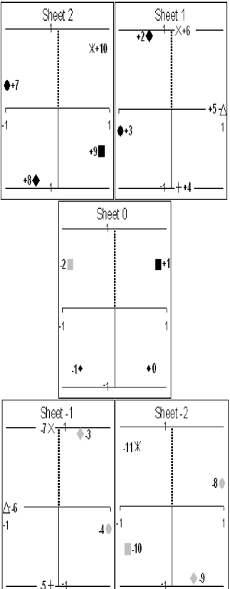
Figure 1: Locations of the turning points for $\epsilon=\frac{12}{5}$. There are 11 $\mathcal{P}\mathcal{T}$-symmetric pairs of turning points, with each pair being mirror images under reflection through the imaginary-$x$ axis on the principal sheet. All 22 turning points lie on the unit circle on a five-sheeted Riemann surface, where the sheets are joined by cuts on the positive-imaginary axis.

As $\epsilon$ increases from 0, the elliptical complex trajectories for the Harmonic oscillator begin to distort. However, the trajectories remain closed and periodic except for special singular trajectories that run off to complex infinity. These singular trajectories only occur when $\epsilon$ is an integer. All of the orbits discussed in Ref. r1 are $\mathcal{P}\mathcal{T}$ symmetric, and it was firmly believed that all closed periodic orbits are $\mathcal{P}\mathcal{T}$ symmetric. (We will see that this is not so, and that non-$\mathcal{P}\mathcal{T}$-symmetric orbits are crucial in understanding the observed rapid variation in the periods of the complex orbits as $\epsilon$ varies slowly.)

In Ref. r1 many complex trajectories $x(t)$ were examined, some having a rich topological structure. Some of these trajectories visit many sheets of the Riemann surface. The classical orbits exhibit fine structure that is exquisitely sensitive to the value of $\epsilon$. Small variations in $\epsilon$ can cause huge changes in the topology and in the periods of the closed orbits. Depending on the value of $\epsilon$, there are orbits having short periods as well as orbits having long and possibly arbitrarily long periods (see Fig. 2).

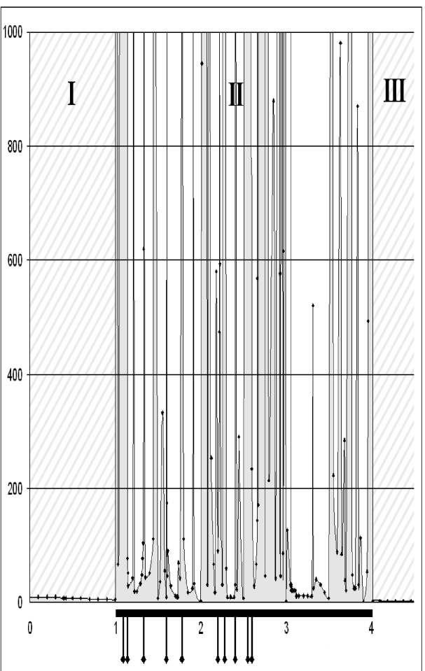
Figure 2: Period of a classical trajectory beginning at the $N=1$ turning point in the complex-$x$ plane. The period is plotted as a function of $\epsilon$. The period decreases smoothly for $0\leq\epsilon<1$ (Region I). However, when $1\leq\epsilon\leq 4$ (Region II), the period becomes a rapidly varying and noisy function of $\epsilon$. For $\epsilon>4$ (Region III) the period is once again a smoothly decaying function of $\epsilon$. Region II contains short subintervals where the period is a small and smoothly varying function of $\epsilon$. At the edges of these subintervals the period suddenly becomes extremely long. Detailed numerical analysis shows that the edges of the subintervals lie at special rational values of $\epsilon$. Some of these special rational values of $\epsilon$ are indicated by vertical line segments that cross the horizontal axis. At these rational values the orbit does not reach the $N=-2$ turning point and the $\mathcal{P}\mathcal{T}$ symmetry of the classical orbit is spontaneously broken.

Figure 2 delineates three regions of $\epsilon$ for which an orbit that begins at the $N=1$ turning point exhibits a specific kind of behavior. When $0\leq\epsilon\leq 1$ (Region I), the period is a smooth decreasing function of $\epsilon$; when $1<\epsilon\leq 4$ (Region II), the period is a rapidly varying and choppy function of $\epsilon$; when $4<\epsilon$ (Region III), the period is once again a smooth and decreasing function of $\epsilon$. For some values of $\epsilon$ in Region II the period is extremely long. Thus, it is difficult to see the behavior of the period in Regions I and III in Fig. 2. We have therefore plotted in Fig. 3 the period for these slowly varying regions.

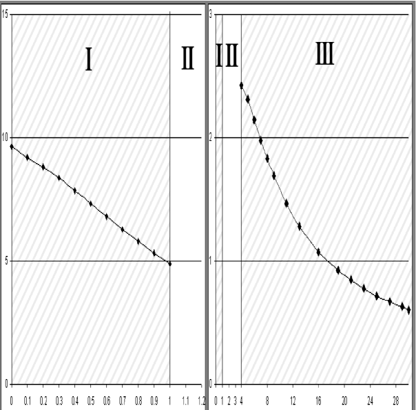
Figure 3: Period of a classical trajectory joining the $K=1$ pair of turning points for $\epsilon$ in Regions I and III. (See Fig. 2.) The orbits in these regions are all $\mathcal{P}\mathcal{T}$ symmetric.

For a trajectory beginning at the $N=2$ turning point, the period as a function of $\epsilon$ again exhibits these three types of behaviors. The period decreases smoothly for $0\leq\epsilon<\textstyle{\frac{1}{2}}$ (Region I). When $\textstyle{\frac{1}{2}}\leq\epsilon\leq 8$ (Region II), the period becomes a rapidly varying and noisy function of $\epsilon$. When $\epsilon>8$ (Region III) the period is once again a smoothly decaying function of $\epsilon$. These behaviors are shown in Fig. 4. Again, because it is difficult to see the dependence of the period in Regions I and III when Region II is included, we display the period for $K=2$ for $\epsilon$ in Regions I and III in Fig. 5. The trajectory terminates at the $N=-3$ turning point except when $\mathcal{P}\mathcal{T}$ symmetry is spontaneously broken. Broken-symmetry orbits occur only at isolated points in Region II.

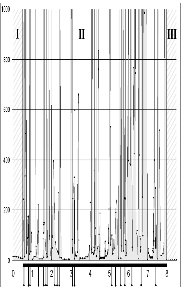
Figure 4: Period of a classical trajectory joining (except when $\mathcal{P}\mathcal{T}$ symmetry is broken) the $K=2$ pair of turning points. The period is plotted as a function of $\epsilon$. As in the $K=1$ case shown in Fig. 2, there are three regions. When $0\leq\epsilon\leq\textstyle{\frac{1}{2}}$ (Region I), the period is a smooth decreasing function of $\epsilon$; when $\textstyle{\frac{1}{2}}<\epsilon\leq 8$ (Region II), the period is a rapidly varying and choppy function of $\epsilon$; when $8<\epsilon$ (Region III), the period is again a smooth and decreasing function of $\epsilon$.

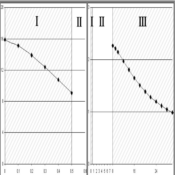
Figure 5: Period of a classical trajectory joining the $K=2$ pair of turning points in the complex-$x$ plane for $\epsilon$ in Regions I and III. (See Fig. 4.)

Figures 2 – 5 illustrate a general pattern that holds for all $K$. For classical orbits that oscillate between the $K$th pair of turning points, there are always three regions. The domain of Region I is $0\leq\epsilon\leq\frac{1}{K}$, the domain of Region II is $\frac{1}{K}<\epsilon<4K$, and the domain of Region III is $4K<\epsilon$. As $\epsilon$ varies, the turning points move in a characteristic fashion for each of these three regions (see Fig. 6). When $\epsilon=0$, the turning points lie on the real axis. As $\epsilon$ increases, the turning points rotate into the complex-$x$ plane. Just as $\epsilon$ reaches the upper edge of Region I, the turning points rotate through an angle of $\frac{\pi}{2}$ and now lie on the imaginary axis. As $\epsilon$ continues to increase, the turning points continue to rotate around $x=0$, and may encircle the origin many times. Just as $\epsilon$ reaches the upper boundary of Region II, the turning points again lie on the real axis. Finally, as $\epsilon$ moves from the lower edge to the upper edge of Region III ($\epsilon=\infty$), the turning points again rotate through an angle of $\frac{\pi}{2}$ and lie on the negative imaginary-$x$ axis.

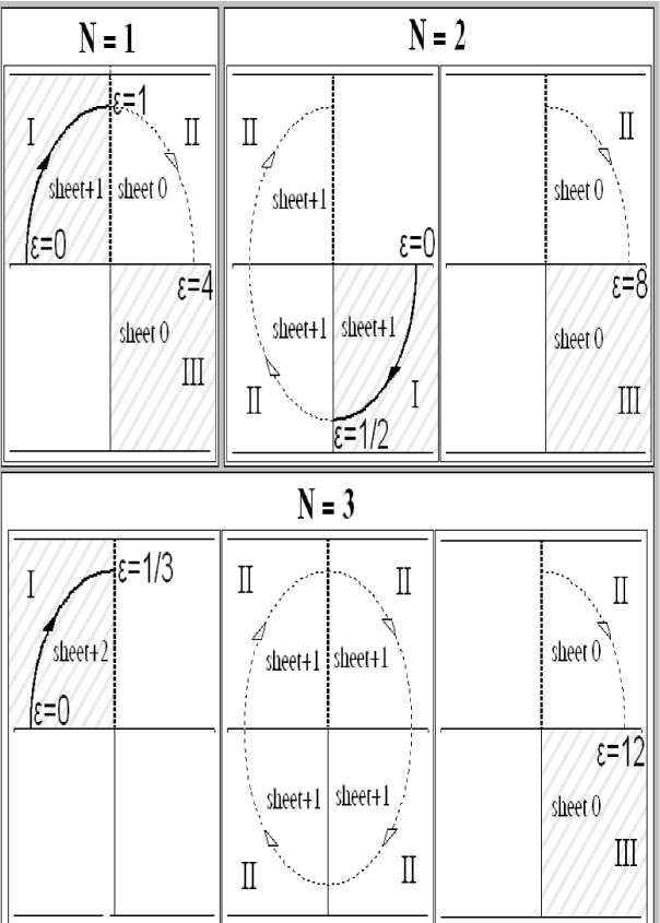
Figure 6: Locations of the turning points in the complex-$x$ plane as $\epsilon$ increases from $0$ to $\infty$. At $\epsilon=0$ the turning points lie on the real-$x$ axis. As $\epsilon$ increases through Region I the turning points rotate through an angle of $\frac{\pi}{2}$ and end up on the imaginary-$x$ axis. As $\epsilon$ increases through Region II, the turning points rotate around the origin and wind up once again on the real axis. Finally, as $\epsilon$ passes through Region III, the turning points again rotate through an angle of $\frac{\pi}{2}$ and finish up on the negative imaginary-$x$ axis.

In general, the period of any classical orbit depends on the specific pairs of turning points that are enclosed by the orbit and on the number of times that the orbit encircles each pair. As explained in Ref. r1 , any orbit can be deformed to a much simpler orbit of exactly the same period. This simpler orbit connects two turning points and oscillates between them rather than encircling them. For the elementary case of orbits that enclose only the $K=0$ pair of turning points, the formula for the period of the closed orbit is

$$T(\epsilon)=2\sqrt{\pi}\frac{\Gamma\left(\frac{3+\epsilon}{2+\epsilon}\right)}{\Gamma\left(\frac{4+\epsilon}{r4+2\epsilon}\right)}\cos\left(\frac{\epsilon\pi}{4+2\epsilon}\right).$$ (4)

The derivation of (4) is straightforward. The period $T$ is given by a closed contour integral along the trajectory in the complex-$x$ plane. This trajectory encloses the square-root branch cut that joins the $K=0$ pair of turning points. This contour can be deformed into a pair of rays that run from one turning point to the origin and then from the origin to the other turning point. The integral along each ray is easily evaluated as a beta function, which is then written in terms of gamma functions. Equation (4) is valid for all $\epsilon\geq 0$.

When the classical orbit encloses more than just the $K=0$ pair of turning points, the formula for the period of the orbit becomes more complicated r1 . In general, there are contributions to the period integral from many enclosed pairs of turning points. We label each such pair by the integer $j$. The general formula for the period of the topological class of classical orbits whose central orbit terminates on the $K$th pair of turning points is

$$T_{K}(\epsilon)=2\sqrt{\pi}\frac{\Gamma\left(\frac{3+\epsilon}{2+\epsilon}\right)}{\Gamma\left(\frac{4+\epsilon}{4+2\epsilon}\right)}\sum_{j=0}^{\infty}a_{j}(K,\epsilon)\left|\cos\left(\frac{(2j+1)\epsilon\pi}{4+2\epsilon}\right)\right|.$$ (5)

In this formula the cosines originate from the angular positions of the turning points in (3). The coefficients $a_{j}(K,\epsilon)$ are all nonnegative integers. The $j$th coefficient is nonzero only if the classical path encloses the $j$th pair of turning points. Each coefficient is an even integer except for the $j=K$ coefficient, which is an odd integer. The coefficients $a_{j}(K,\epsilon)$ satisfy

$$\sum_{j=0}^{\infty}a_{j}(K,\epsilon)=k,$$ (6)

where $k$ is the number of times that the central classical path crosses the imaginary axis. Equation (6) truncates the summation in (5) so that it contains a finite number of terms.

As we can see in Figs. 2 and 4, for an orbit that oscillates between the $K$th pair of turning points ($K>0$) the classical behavior undergoes abrupt transitions as $\epsilon$ is varied smoothly in Region II. In Region II there are narrow patches in which the period of the orbit is rapidly varying which are sandwiched between small regions of quiet stability. At the boundaries of the slowly varying and rapidly varying regions there are transitions in the topologies and periods of the classical orbits. We can understand from (5) how there can be rapid variations in the period of the orbit. The summation in (5) can vary rapidly as a function of $\epsilon$ because small changes in $\epsilon$ can cause fluctuations in the topology of the orbit. If the orbit suddenly encloses many more pairs of turning points, the value of the period may fluctuate wildly. [Note that abrupt changes in the periods of the orbits cannot occur for the trajectories joining the $K=0$ pairs of turning points because $T(\epsilon)$ in (4) is a smoothly decreasing function for all $\epsilon\geq 0$.]

III Classical Orbits Having Broken $\mathcal{P}\mathcal{T}$ Symmetry

We now demonstrate that the abrupt changes in the topology and the periods of the orbits that we observe for $\epsilon$ in Region II are associated with the appearance of orbits having spontaneously broken $\mathcal{P}\mathcal{T}$ symmetry. In Region II there are short patches where the period is relatively small and is a slowly varying function of $\epsilon$. These patches are bounded by special values of $\epsilon$ for which the period of the orbit suddenly becomes extremely long. From our numerical studies of the orbits connecting the $K$th pair of turning points, we believe that there are only a finite number of these special values of $\epsilon$ and that these values of $\epsilon$ are always rational. Furthermore, we have discovered that at these special rational values of $\epsilon$, the closed orbits are not $\mathcal{P}\mathcal{T}$-symmetric and we say that such orbits exhibit spontaneously broken $\mathcal{P}\mathcal{T}$ symmetry. Some special values of $\epsilon$ at which spontaneously broken $\mathcal{P}\mathcal{T}$-symmetric orbits occur are indicated in Figs. 2 and 4 by short vertical lines below the horizontal axis. These special values of $\epsilon$ always have the form $\frac{p}{q}$, where $p$ is a multiple of 4 and $q$ is odd.

Figure 7 displays an orbit having spontaneously broken $\mathcal{P}\mathcal{T}$ symmetry. This orbit occurs when $\epsilon=\frac{4}{5}$. The orbit starts at the $N=2$ turning point, but it never reaches the $\mathcal{P}\mathcal{T}$-symmetric turning point $N=-3$. Rather, the orbit terminates when it runs into and is reflected back from the complex conjugate $N=4$ turning point [see (3)]. Thus, a broken-$\mathcal{P}\mathcal{T}$-symmetric orbit is a failed $\mathcal{P}\mathcal{T}$-symmetric orbit. The period of the orbit is short ($T=4.63$). This orbit is not $\mathcal{P}\mathcal{T}$ (left-right) symmetric but it does possess complex-conjugate (up-down) symmetry. In general, for a non-$\mathcal{P}\mathcal{T}$-symmetric orbit to exist, it must join or encircle a pair of complex-conjugate turning points.

Figure 7: A horseshoe-shaped non-$\mathcal{P}\mathcal{T}$-symmetric orbit. This orbit is not symmetric with respect to the imaginary axis but it is symmetric with respect to the real axis. The orbit terminates at a complex-conjugate pair of turning points. For this orbit, $\epsilon=\frac{4}{5}$.

If we change $\epsilon$ slightly, $\mathcal{P}\mathcal{T}$ symmetry is restored and one can only find orbits that are $\mathcal{P}\mathcal{T}$ symmetric. For example, if we take $\epsilon=0.805$, we obtain the complicated orbit in Fig. 8. The period of this orbit is large ($T=173.36$).

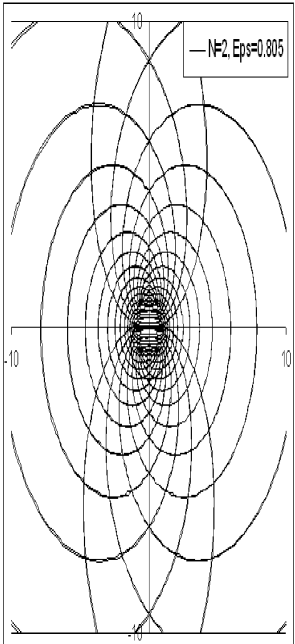
Figure 8: $\mathcal{P}\mathcal{T}$-symmetric orbit for $\epsilon=0.805$. This orbit connects the $K=2$ pair of turning points.

It is possible to have more than one kind of broken-$\mathcal{P}\mathcal{T}$-symmetric orbit for a given rational value of $\epsilon$. For example, in Figs. 9 and 10 we display two different non-$\mathcal{P}\mathcal{T}$-symmetric closed orbits for $\epsilon=\frac{12}{5}$. In Fig. 9 the horseshoe-shaped orbit terminates on the $N=3$ and $N=7$ turning points. The period of this orbit is ($T=5.04$). The more complicated orbit shown in Fig. 10 terminates on the $N=2$ and $N=8$ turning points. The period of this orbit is $T=12.90$. All of these turning points are shown in Fig. 1 .

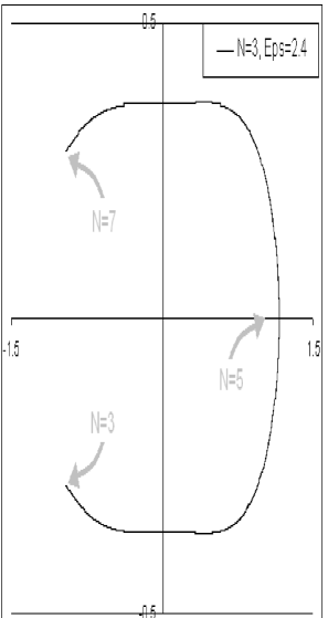
Figure 9: A non-$\mathcal{P}\mathcal{T}$-symmetric horseshoe-shaped orbit for $\epsilon=\frac{12}{5}$. This orbit begins at the $N=3$ turning point and terminates at the $N=7$ turning point, so that it fails to reach the $\mathcal{P}\mathcal{T}$-symmetric turning point at $N=-4$. These turning points are shown in Fig. 1. The period of this orbit is $T=5.04$.

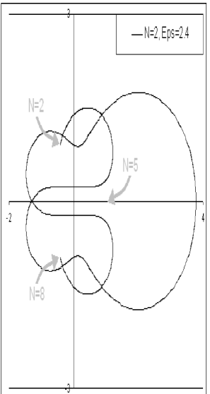
Figure 10: A non-$\mathcal{P}\mathcal{T}$-symmetric orbit for $\epsilon=\frac{12}{5}$. This orbit, which is more complicated than that shown in Fig. 9, begins at the $N=2$ turning point and ends at the $N=8$ turning point before it can reach the $\mathcal{P}\mathcal{T}$-symmetric turning point at $N=-3$. These turning points are shown in Fig. 1. The period of this orbit is $T=12.90$.

A non-$\mathcal{P}\mathcal{T}$-symmetric orbit that is even more complicated than that in Fig. 10 is shown in Fig. 11. This orbit connects the $N=2$ and $N=48$ turning points for $\epsilon=\frac{76}{13}$.

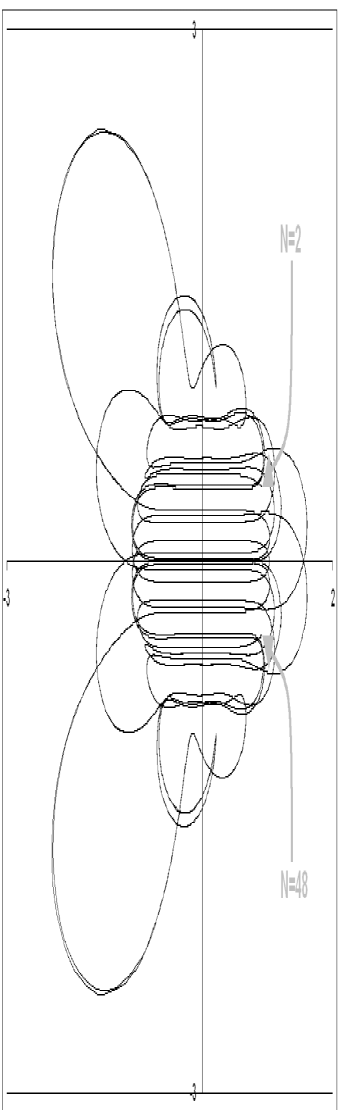
Figure 11: A broken-$\mathcal{P}\mathcal{T}$-symmetric orbit connecting the $N=2$ and $N=48$ turning points for $\epsilon=\frac{76}{13}$. The period of this orbit is $T=78.36$.

Non-$\mathcal{P}\mathcal{T}$-symmetric orbits can encircle a complex-conjugate pair of turning points as well as terminating at them. In Fig. 12 two non-$\mathcal{P}\mathcal{T}$-symmetric orbits are shown for $\epsilon=\frac{8}{5}$. One orbit joins the $N=1$ and $N=7$ complex-conjugate pair of turning points. The other orbit encircles these turning points. Both orbits have the same period of $T=9.07$.

Figure 12: Two non-$\mathcal{P}\mathcal{T}$-symmetric orbits of the same period $T=9.07$. The value of $\epsilon$ is $\frac{8}{5}$. The solid-line orbit terminates at the $N=1$ and $N=7$ turning points, while the dotted-line orbit encircles these turning points.

Broken-$\mathcal{P}\mathcal{T}$-symmetric orbits can have an elaborate topology. For example, at $\epsilon=\frac{16}{9}$ we find a non-$\mathcal{P}\mathcal{T}$-symmetric orbit whose topology is even more complicated than that of the orbit shown in Fig. 11. This orbit, which is shown in Fig. 13, is a failed $K=3$ $\mathcal{P}\mathcal{T}$-symmetric orbit. It originates at the $N=-4$ turning point, but it never reaches the $\mathcal{P}\mathcal{T}$-symmetric $N=3$ turning point. This is because it is reflected back by the complex-conjugate $N=-14$ turning point. Figure 14 shows the $\mathcal{P}\mathcal{T}$-symmetric companion of the orbit in Fig. 13. This orbit begins at the $N=3$ turning point, but is reflected back by the $N=13$ turning point, which is the $\mathcal{P}\mathcal{T}$ counterpart of the $N=-14$ turning point.

Figure 13: Non-$\mathcal{P}\mathcal{T}$-symmetric orbit for $\epsilon=\frac{16}{9}$. This topologically complicated orbit originates at the $N=-4$ turning point but does not reach the $\mathcal{P}\mathcal{T}$-symmetric $N=3$ turning point. Instead, it is reflected back at the complex-conjugate $N=-14$ turning point. The period of this orbit is $T=186.14$).

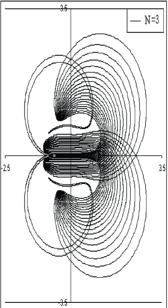
Figure 14: $\mathcal{P}\mathcal{T}$-symmetric reflection of the orbit in Fig. 13. This orbit originates at the $N=3$ turning point but is reflected back by the $N=13$ turning point.

To show that the orbits in Figs. 13 and 14 are $\mathcal{P}\mathcal{T}$ reflections, we have plotted both orbits in Fig. 15. The left-right symmetry is manifest. A definitive demonstration of the symmetry can be given by plotting the complex argument of $x(t)$ as a function of time $t$ for each orbit. This is done in Fig. 16.

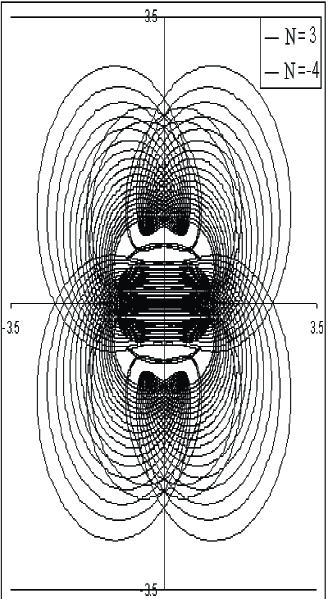
Figure 15: Superposition of the orbits in Figs. 13 and 14. The $\mathcal{P}\mathcal{T}$ (left-right) symmetry is exact.

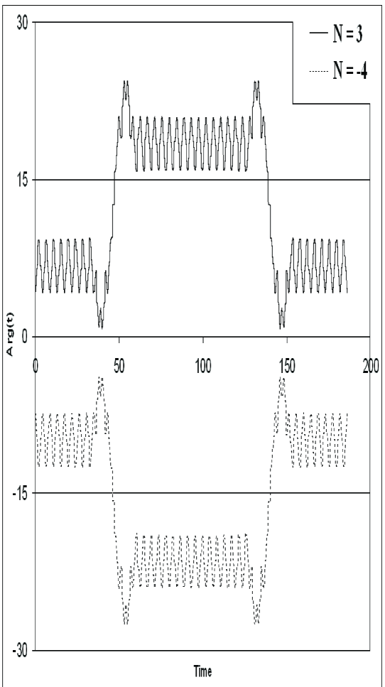
Figure 16: The complex argument of $x(t)$ plotted as a function of $t$ for the non-$\mathcal{P}\mathcal{T}$-symmetric orbits in Figs. 13 and 14. The two plots verify that the two orbits are $\mathcal{P}\mathcal{T}$-symmetric reflections of one another.

Finally, we display in Fig. 17 a spontaneously broken-$\mathcal{P}\mathcal{T}$-symmetric orbit that is vastly more complicated than those shown in Figs. 13 and 14. This orbit begins at the $N=1$ turning point for $\epsilon=\frac{16}{15}$. It terminates at the complex conjugate $N=21$ turning point rather than at the $\mathcal{P}\mathcal{T}$-symmetric $N=-2$ turning point. The period of this orbit is $T=3393.64$.

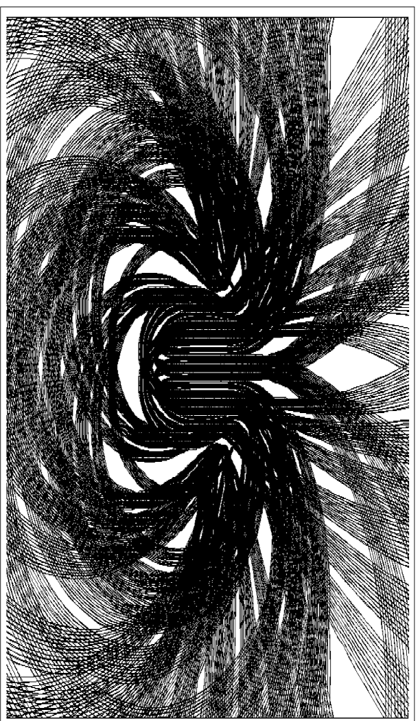
Figure 17: A non-$\mathcal{P}\mathcal{T}$-symmetric orbit having an extremely elaborate topology. The value of $\epsilon$ for this orbit is $\frac{16}{15}$. The orbit originates at the $N=1$ turning point and terminates at the complex-conjugate $N=21$ turning point. This orbit visits eight of the fifteen sheets of the Riemann surface and travels a great distance from the origin. Only the $-2<{\rm Re}\,x<2$, $-2<{\rm Im}\,x<2$ portion of the complex-$x$ plane is shown.

IV Concluding Remarks

The work in Ref. r1 provides a heuristic explanation of how very long-period orbits arise. In order for a classical trajectory to travel a great distance in the complex plane, its path must slip through a forest of turning points. When the trajectory comes under the influence of a turning point, it usually executes a huge number of nested U-turns and eventually returns back to its starting point. However, for some values of $\epsilon$ the complex trajectory may evade many turning points before it eventually encounters a turning point that takes control of the particle and flings it back to its starting point. We speculated in Ref. r1 that it may be possible to find special values of $\epsilon$ for which the classical path manages to avoid and sneak past all turning points. Such a path would have an infinitely long period. (We still do no know if such infinite-period orbits exist.)

However, in Ref. r1 we could not provide an explanation of why the period of a closed trajectory, as a function of $\epsilon$, is such a wildly fluctuating function. We have shown here that for special rational values of $\epsilon$ the trajectory bumps directly into a turning point that is located at a point that is the complex conjugate of the point from which the trajectory was launched. This turning point reflects the trajectory back to its starting point and prevents the trajectory from being $\mathcal{P}\mathcal{T}$ symmetric. Trajectories for values of $\epsilon$ near these special rational values have extremely different topologies and thus have periods that tend to be relatively long. This explains the noisy plots in Figs. 2 and 4.

Figs. 7 and 8 illustrate this phenomenon. The value of $\epsilon$ for Fig. 7 differs from that in Fig. 8 by only $0.005$. Nevertheless, the orbits in these two figures exhibit very different topologies. This is because the trajectory in Fig. 7 is a failed $\mathcal{P}\mathcal{T}$-symmetric orbit, where the trajectory that starts at the $N=2$ turning point is reflected almost immediately by the complex-conjugate $N=4$ turning point. When $\epsilon$ is changed by the tiniest amount, the turning points are slightly displaced. As a result, the trajectory in Fig. 8 manages to sneak past the $N=4$ turning point and travels a great distance in the complex plane before bouncing back from the $\mathcal{P}\mathcal{T}$-symmetric $N=-3$ turning point.

We do not know whether for each turning point there are a finite or an infinite number of special rational values of $\epsilon$ for which the classical orbit has a broken $\mathcal{P}\mathcal{T}$ symmetry. It is worth noting that the data used to produce Figs. 2 and 4 is far from exhaustive and that the bars underneath the horizontal axes are only the known examples of broken $\mathcal{P}\mathcal{T}$ symmetry. There are surely many more such special rational values of $\epsilon=\frac{p}{q}$. In this paper we concluded our study at $q=13$, and this work took an immense amount of computer time!

The study of complex trajectories for classical dynamical systems is a rich new area in mathematical physics that deserves extensive analytical and numerical exploration. Already, there has been work done on the complex orbits of the simple pendulum r7 , the complex extension of the Korteweg-de Vries equation r8 ; r9 , complex solutions of the Euler equations for rigid-body rotation r10 , and the complex version of the kicked rotor r11 . We expect that complex analysis will provide a deep insight into the behavior of dynamical systems.

- (1) C. M. Bender, J.-H. Chen, D. W. Darg, and K. A. Milton, J. Phys. A: Math. Gen. 39, 4219 (2006).
- (2) On the website http://users.ox.ac.uk/rege0582/ there is a java applet that can be used to plot the classical trajectories displayed in this paper.
- (3) C. M. Bender and S. Boettcher, Phys. Rev. Lett. 80, 5243 (1998).
- (4) P. Dorey, C. Dunning, and R. Tateo, J. Phys. A: Math. Gen. 34, L391 (2001) and 34, 5679 (2001).
- (5) C. M. Bender, D. C. Brody, and H. F. Jones, Phys. Rev. Lett. 89, 270401 (2002).
- (6) C. M. Bender, S. Boettcher, and P. N. Meisinger, J. Math. Phys. 40, 2201 (1999).
- (7) A. Nanayakkara, Czech. J. Phys. 54, 101 (2004) and J. Phys. A: Math. Gen. 37, 4321 (2004).
- (8) C. M. Bender, D. D. Holm, and D. W. Hook, J. Phys. A: Math. Theor. 40, F81 (2007).
- (9) C. M. Bender, D. C. Brody, J.-H. Chen, and E. Furlan, J. Phys. A: Math. Theor., to appear [arXiv: math-phys/0610003].
- (10) A. Fring [arXiv:math-ph/0701036].
- (11) C. M. Bender, D. D. Holm, and D. W. Hook, in preparation.
- (12) C. M. Bender, J. Feinberg, and D. W. Hook, in preparation.