March 8, 2007

DAMTP-07-15

hep-th/0703068

Geometry and topology of bubble solutions from gauge theory

Heng-Yu Chen¹, Diego H. Correa¹ and Guillermo A. Silva^2
1DAMTP, Centre for Mathematical Sciences
University of Cambridge, Wilberforce Road
Cambridge CB3 0WA, UK
and
²Departmento de Física
Universidad Nacional de La Plata
CC 67, 1900, La Plata, Argentina

Abstract

We study how geometrical and topological aspects of certain $\frac{1}{2}$-BPS type IIB supergravity solutions are captured by the ${\cal N}=4$ Super Yang-Mills gauge theory in the AdS/CFT context. The type IIB solutions are completely characterized by arbitrary droplets in a plane and we consider, in particular, concentric droplets. We probe the dual $\frac{1}{2}$-BPS operators of the gauge theory with single traces and extract their one-loop anomalous dimensions. The action of the one-loop dilatation operator can be reformulated as the Hamiltonian of a bosonic lattice. The operators defining the Hamiltonian encode the topology of the droplet. The axial symmetry of the droplets turns out to be essential for obtaining the spectrum of the Hamiltonians. In appropriate BMN limits, the near-BPS spectrum reproduces the spectrum of near-BPS string excitations propagating along each individual edge of the droplet of the dual geometric background. We also study semiclassical regimes for the Hamiltonians. We show that for droplets having disconnected constituents, the Hamiltonian admits different complimentary semiclassical descriptions, each one replicating the semiclassical description for closed strings extending in each of the constituents.

1 Introduction

The notion of emergent geometry in the AdS/CFT correspondence [1] holds certain appeal. The general idea is that judicial choices of BPS operators in the gauge theory are capable of encoding the characteristics of the corresponding dual geometries [2, 3].

A paradigmatic example was provided by [2], focusing on the $\frac{1}{2}$-BPS operators of $\mathcal{N}=4$ SYM constructed exclusively from a complex adjoint chiral scalar $Z$. The dynamics of this sub-sector can be described by gauged harmonic oscillators, which in turn can be mapped into a Fermi problem. The ground state of the system corresponds to a completely occupied Fermi sea forming a disc in the phase space. This distribution, known as the droplet, can then be associated, at the semi-classical level, with the allowed eigenvalues of the scalar field $Z$ [2]. Other $\frac{1}{2}$-BPS ‘excitations’ correspond to disc distortions, further splitting into isolated droplets and creation of holes within these droplets. All these lead to droplets with non-trivial shapes and topologies [3, 4, 5, 6]. This class of $\frac{1}{2}$-BPS states preserve 16 supersymmetries as well as a bosonic $R\times SO(4)\times SO(4)$ symmetry group. The dual type IIB supergravity backgrounds, known as Lin-Lunin-Maldacena (LLM) geometries, were constructed by fibering two $S^{3}$ over a two dimensional plane [3]. The base of the fibration in this construction was proposed to be identified with the droplets describing the eigenvalue distribution in the gauge theory. In particular, the $AdS_{5}\times S^{5}$ geometry is shown to correspond to a circular disc droplet, whereas single particle and hole creations were identified with the nucleations of a giant graviton in $AdS_{5}$ and $S^{5}$ respectively [2, 3]. The bottom line of the construction is that when the number of giant gravitons becomes large, the back-reacted non-singular geometry gets parameterized in terms of a single scalar function obeying a Laplace-like differential equation whose boundary conditions on a two dimensional plane can only take the values $\pm\frac{1}{2}$.

Generically, a probe closed string propagating on a LLM geometry should be seen in the dual gauge field theory as a non-BPS operator given by a single trace operator describing the excitations (probe string) on top of a $\frac{1}{2}$-BPS operator (LLM geometry). The study of the one-loop anomalous dimensions for such gauge theory operators turns out to be very rewarding. For the case of simply connected droplets, the gauge theory Hamiltonian describing probe strings was recently derived [7]. This Hamiltonian can be written in terms of certain operators obeying an algebra that encodes, in a simple fashion, the moments describing the geometry of the droplet. Moreover, using the coherent state basis for the operators, a semi-classical action was derived, from which it was possible to reconstruct the region of the LLM droplet plane where the dual string propagates [7]. The approach described in [7, 8, 9] is similar in spirit to the coherent state approach in the context of spin-chain/spinning string correspondence [10, 11], where the coherent state action for the integrable spin chain Hamiltonian [12] was identified with the spinning-string action in certain “fast-string” limit.

Making the existing picture more precise is the focus of our paper. In particular, we will obtain quantitative information about the dual metric, for droplets of general shapes and topologies, from gauge theory computations. For definiteness we will consider non-BPS excitations, or string probe states, in topologically non-trivial LLM backgrounds, evaluate their scaling dimensions and importantly, distinguish them from their counterparts in $AdS_{5}\times S^{5}$. From the dual gauge theory perspective, the key steps towards these aims amount to defining the appropriate field theory operators and compute the action of the dilatation operator whose eigenvalues give the scaling dimensions.

The generalization we carry out is interesting since the geometric backgrounds we consider are topologically different from $AdS_{5}\times S^{5}$ or any LLM geometries associated with simply connected droplets. In this regard, it is important to understand how topology is revealed from purely gauge theory means. In particular, the appearance of additional edges for the droplet indicates the existence of new disconnected sets of null geodesics in the geometry. Let us recall that for the case of circular disc, BPS and near-BPS string excitations are represented by single traces having a large number $J$ of complex chiral scalar fields $Z$ [13], furthermore these excitations get localized at the unique edge of the circular droplet [3]. When droplets with multiple edges are considered, one should identify new types of excitations and argue how they get localized at each individual edge. Another appealing situation to consider are the non-connected droplets, since one should then identify within the gauge theory the operators dual to strings whose propagations are restricted to each disconnected droplet.

The simplest setup for studying multiple edges and disconnected droplets is that of concentric droplets. An advantageous feature of these axially symmetric droplets is that the dual LLM geometry defining functions are explicitly given as superposition of uniform discs. The one-loop Hamiltonian we will derive on the gauge theory side corresponding to strings probing concentric LLM geometries, will be seen as the Hamiltonian of a bosonic lattice along the lines of [7, 8, 9]. Interestingly, the axial symmetry of the droplets will be essential for finding the Hamiltonian spectrum.

The rest of the paper is organized as follows: In section 2 we present the $\frac{1}{2}$-BPS operators we will be working with: they are characterized by a concentric distribution of eigenvalues and as should become clear dual to concentric LLM geometries. In section 3 we excite them with single traces. We focus on two particular cases: the annular droplet which is connected but has two edges and a droplet consisting of a disc and a disconnected annulus. We then derive the Hamiltonians corresponding to the one-loop anomalous dimension operators for non-BPS excited states. By taking appropriate BMN-like limits, we show the spectra of these Hamiltonians precisely match with the spectra of the corresponding dual string states. Furthermore, by considering the semi-classical coherent state action for these Hamiltonians, we show the agreement with the Polyakov action of the dual string solution in certain fast-string limit. We summarize and discuss potential research directions in section 4. In an appendix, we include details on LLM geometries as well as their BMN limits; we also list some semi-classical string solutions in backgrounds constructed from concentric droplets.

2 Concentric droplets

Half-BPS states of $U(N)$ ${\cal N}=4$ SYM can be described in terms of a gauged $N\times N$ normal matrix model with a harmonic oscillator potential [2, 14]. Each supersymmetric state is associated to a wave-function of the normal matrix model. The normalization of each BPS state coincides with the partition function of a random matrix model for a particular ensemble $W$,

$$\int\prod_{i=1}^{N}d^{2}z_{i}\,|\psi(z)|^{2}=\int\prod_{i=1}^{N}d^{2}z_{i}\,\exp\left(\sum_{j}W(z_{j},\bar{z}_{j})+2\sum_{j<k}\log|z_{j}-z_{k}|\right)\,.$$ (1)

The logarithm in the exponential is attributed to the Van Der Monde determinant, which arises from writing the integration measure in terms of the eigenvalues of the matrices (see [15] for a review) and is the origin of the system becoming fermionic. One effectively ends up with a system consisting on $N$ one-dimensional fermions.

The gauge theory ground state, which is dual to the $AdS_{5}\times S^{5}$ geometry, corresponds to the gaussian ensemble, i.e.

$$W(z,\bar{z})=-|z|^{2}\,.$$ (2)

In the large $N$ limit, the semi-classical continuum approximation to the matrix model partition function (1) leads to a characterization of the states in terms of a density distribution of eigenvalues $\rho$ defined on a two dimensional plane. The support of the density distribution determines what we call the droplets. For the gaussian potential (2), the saddle point analysis shows that the partition function (1) is dominated by a uniform distribution of eigenvalues on a disc of radius $\sqrt{N}$ centered at the origin [15].

Arbitrary $\frac{1}{2}$-BPS states are constructed as ‘excitations’ above the ground state and can be represented as [2, 5]

$$|\psi\rangle=\exp\left({\rm tr}\left(\Omega(Z)\right)\right)|\psi_{0}\rangle\,.$$ (3)

The corresponding normalization is again a matrix model partition function, but with the potential ensemble $W$ now generalizes to:

$$W(z,\bar{z})=-|z|^{2}+\Omega(z)+\overline{\Omega(z)}\,.$$ (4)

A harmonic $\Omega(z)$ function guarantees that in the large $N$ limit, the system continues to be dominated by a uniform distribution of eigenvalues, with the droplet shape depending on the potential ensemble $W$. BPS states corresponding to polynomial potentials and their string excitations have recently been studied in [7].

Exciting the ground state with the operator $\det(Z-\lambda)$ induces a potential $\Omega(z)=\log(z-\lambda)$, which generates a hole in the circular droplet at complex position $\lambda$ [2, 5]. This corresponds on the string side to a single non-back-reacting spherical giant graviton in the $AdS$ bulk. In order to obtain a hole of size comparable to the area of the droplet and create a back-reacted geometry, the number of giant gravitons needs to be comparable to $N$. Hence we need to excite the ground state with a product of $M\simeq{\cal O}(N)$ determinants. We will thus consider a density distribution of holes $\sigma(\lambda)$ giving the potential

$$\Omega(z)=\int d^{2}\lambda\ \sigma(\lambda)\log(z-\lambda)\,.$$ (5)

An important example is the following: Take $\sigma(\lambda)$ to be $\frac{1}{\pi}$ in the interior of a disc $D$ of radius $R_{1}=\sqrt{M}$ centered at the origin and zero elsewhere, the potential $W$ takes the form

$$W(z,\bar{z})=-|z|^{2}+\frac{2}{\pi}\int_{D}d^{2}\lambda\ \log|z-\lambda|\,.$$ (6)

The second term in (6) is nothing but the electrostatic potential in a two-dimensional plane due to an uniformly charged disc. Performing the integral, the potential (6) reads

$$W(z,\bar{z})=\left\{\begin{array}[]{c l}0&{\rm if}\ |z|\leq R_{1}\\ -|z|^{2}+R_{1}^{2}(1+2\log(|z|/R_{1}))&{\rm if}\ |z|>R_{1}\end{array}\right.$$ (7)

The random matrix problem with potential (7) is tractable even for finite $N$, we will nevertheless be interested in the large $N$ limit later.

Let $\rho(z)$ be the eigenvalues distribution, its mean value in the matrix model (1) is given by (see [15] for a review)

$$\langle\rho(z)\rangle_{N}=e^{W(|z|)}\sum_{i=0}^{N-1}\frac{|z|^{2i}}{h_{i}}\,,$$ (8)

and for the axially symmetric potentials, the constants $h_{i}$ are given by

$$\int d^{2}z\ z^{i}\overline{z}^{j}e^{W(z,\bar{z})}=h_{i}\delta_{ij}\,.$$ (9)

The potential (7) gives

$$h_{i}=\frac{R_{1}^{2i+2}}{i+1}+\left(\frac{e}{R_{1}^{2}}\right)^{R_{1}^{2}}\Gamma(n+1+R_{1}^{2},R_{1}^{2})\,.$$ (10)

Here $\Gamma(a,x)$ is the incomplete gamma function. Plotting (8) for different values of $N$ and $R_{1}$, it is easy to see that, as $N$ and $R_{1}^{2}$ are taken large, $\langle\rho(z)\rangle_{N}$ approaches $1/\pi$ for $R_{1}<|z|<\sqrt{R_{1}^{2}+N}$ or zero otherwise (see Figure 1).

Figure 1: Eigenvalue distributions for $N=1200$ and $M=400$ for: (left) homogeneously distributed holes on a disc and (right) all holes placed at the origin.

Let us analyze the continuum (large $N$) limit for an arbitrary distribution of holes $\sigma(\lambda)$. In other words, consider a state obtained by the product of $M\sim{\mathcal{O}}(N)$ determinants at arbitrary positions $\lambda_{\alpha}$ exciting the ground state,

$$|\psi\rangle=\prod_{\alpha=1}^{M}\det(Z-\lambda_{\alpha})|\psi_{0}\rangle\,.$$ (11)

The integrand in (1) then takes the form

$$|\psi|^{2} \!=\! \exp\left(-\int\!d^{2}\!z\,|z|^{2}\rho(z)+2\int\!\!\int\!d^{2}\!z\,d^{2}\!\lambda\,\rho(z)\sigma(\lambda)\log|z-\lambda|\right.{}$$ (12)

$$\qquad\qquad+\left.\int\!\!\int\!d^{2}\!z\,d^{2}\!{z^{\prime}}\rho(z)\rho(z^{\prime})\log|z-z^{\prime}|\right)\,,$$

where the eigenvalue and hole density distributions $\rho(z)$ and $\sigma(z)$ are constrained to satisfy

$$\int\!d^{2}\!z\,\rho(z)=N\,,\qquad\int\!d^{2}\!z\,\sigma(z)=M\,.$$ (13)

The normalization (12) is dominated by the eigenvalue distribution $\rho(z)$ maximizing the exponential. Taking a variation with respect to $\rho(z)$, one is led to the following equation of motion,

$$-|z|^{2}+2\!\int\!d^{2}\!\lambda\,\sigma(\lambda)\log|z-\lambda|+2\!\int\!d^{2}\!{z^{\prime}}\rho(z^{\prime})\log|z-z^{\prime}|=0\,.$$ (14)

Now, acting on (14) with the two-dimensional Laplace operator we get a consistency equation:

$$-4+4\pi\sigma(z)+4\pi\rho(z)=0\,.$$ (15)

This equation justifies the selection $\sigma(z)=\frac{1}{\pi}$ in (6). Choosing the hole density $\sigma(z)$ to be exclusively $1/\pi$ or zero guarantees having no partially filled regions. The droplet density $\rho(z)$ vanishes in the region where the hole density $\sigma(z)$ takes the value $1/\pi$, and takes the value $1/\pi$ where $\sigma(z)$ vanishes. This choice is the dual version of the one appearing on the gravity side ensuring singularity free geometries [3].

In the example discussed above (equations (6)-(7)), $\sigma(z)$ was taken to be constant over a disc of radius $R_{1}$, and as result the eigenvalues got distributed in an annular domain with radii $R_{1}=\sqrt{M}$ and $R_{2}=\sqrt{M+N}$. However, the potential (6) leading to the uniform annular eigenvalue distribution is not unique in the large $N$ limit. Alternatively, consider exciting the ground state with $\det(Z)^{M}$, which corresponds to placing all the holes at the origin, leads to $h_{n}=(n+M)!$ and the eigenvalue distribution,

$$\langle\rho(z)\rangle_{N}=e^{-|z|^{2}}|z|^{2M}\sum_{i=0}^{N-1}\frac{|z|^{2i}}{(i+M)!}\,,$$ (16)

which is only distinguishable from (8) for finite values of $N$ and $M$ (see Figure 1).

Let us summarize here, a general concentric droplet can be generated by exciting the ground state with the operator

$${\cal O}^{(BPS)}_{LLM}\!\! = \!\!\prod_{\alpha=1}^{M}\det(Z-\lambda_{\alpha})=\prod_{\alpha_{1}=1}^{M_{1}}\!\!\det(Z-\lambda_{\alpha_{1}})\dots\!\!\prod_{\alpha_{k}=1}^{M_{k}}\!\!\det(Z-\lambda_{\alpha_{k}}).$$ (17)

where each set $\{\lambda_{\alpha_{n}}\}$ of $M_{n}$ holes are distributed homogeneously in circles of radius $r_{n}$. The resulting eigenvalue distribution is a series of disconnected annuli centered at the origin. It would be interesting to better understand the relation between the operators ${\cal O}^{(BPS)}_{LLM}$ and the Young Tableaux [2, 14]. For the time being, what is relevant to us is that in the large $N$ limit (17) leads to concentric eigenvalue distributions

3 String excitations in concentric droplets

In the previous section we have seen how certain BPS operators are associated to droplet pictures in a plane. These operators are believed to be dual to some supergravity solutions with exactly the same quantum numbers, and moreover these solutions are also characterized by identical droplet pictures. A skeptical reader might object that only qualitative evidence supports this identification. In this section we will show that by probing these BPS operators with a non-BPS factor it is possible to reconstruct some geometrical and topological information of the dual LLM geometry.

We will consider single traces probing the BPS operators associated with the concentric droplets of the previous section and interpret them as closed string probes of concentric LLM backgrounds. We will take the probing single traces to be in the so-called $SU(2)$ sub-sector of ${\mathcal{N}}=4$ SYM, that is, in addition to the chiral $Z$ fields they also contain complex chiral scalar fields $Y$. The resulting excited operators are generically non-BPS and the study of their anomalous dimensions will substantiate their identification with closed string excitations.

To one-loop order, the dilatation operator in the $SU(2)$ sub-sector is given by [17]

$$D=D_{0}+\lambda D_{1}+{\cal O}(\lambda^{2})\,,$$ (18)

here $\lambda=\frac{g^{2}N}{8\pi^{2}}$ is the ’t Hooft coupling, $D_{0}={\rm tr}(Z\partial_{Z}+Y\partial_{Y})$ gives the classical dimension and the one-loop anomalous dimension operator $D_{1}$ can be written in the form,

$$D_{1}=N^{-1}{\rm tr}([Z,Y][\partial_{Z},\partial_{Y}])\,.$$ (19)

The action of the $D_{1}$ on the set of operators of the form ${\cal O}=\mathrm{tr}(ZY...){\cal O}^{(BPS)}_{LLM}$ receives two contributions, the first comes from the action of $\partial_{Z}$ (as well as $\partial_{Y}$) on the trace representing the string. The second contribution comes from the action of $\partial_{Z}$ on the product of determinants ${\cal O}^{(BPS)}_{LLM}$. The action of $\partial_{Z}$ on the product of determinants gives a sum over the $\lambda_{\alpha_{n}}$, which, in the continuous limit, can in turn be approximated by contour integrals in the complex plane. The result is

$$\!\!\!(\partial_{Z})^{i}_{j}{\cal O}^{(BPS)}_{LLM}\!\!\! = \!\!(\partial_{Z})^{i}_{j}\!\!\prod_{\alpha_{1}=1}^{M_{1}}\!\!\det(Z-\lambda_{\alpha_{1}}\!)...\!\!\prod_{\alpha_{k}=1}^{M_{k}}\!\!\det(Z-\lambda_{\alpha_{k}}\!)$$ (20)

$$= (M_{1}{(P_{1})}^{i}_{j}+...+M_{k}{(P_{k})}^{i}_{j}){\cal O}^{(BPS)}_{LLM}\,,$$

where

$$P_{n}=\frac{1}{M_{n}}\sum_{\alpha=1}^{M_{n}}\frac{1}{Z-\lambda_{\alpha}}\simeq\frac{1}{2\pi i}\oint_{|\lambda|=r_{n}}\frac{d\lambda}{\lambda(Z-\lambda)}\,.$$ (21)

We will see below that the matrix $P_{n}$ effectively projects the string excitations to the droplets lying outside $r_{n}$.

Let us begin by analyzing the doubly-connected annular domain, which can be generated, as discussed at the end of previous section, by exciting the vacuum with ${\cal O}^{(BPS)}_{LLM}=\det(Z)^{M}$. In this case (20) reduces to

$$(\partial_{Z})^{i}_{j}\,\det(Z)^{M}=M{(Z^{-1})}^{i}_{j}\,\det(Z)^{M}\,,$$ (22)

A closed string excitation on the annular LLM geometry is represented by a single trace operator on top of the product of determinants. Instead of the usual spin chain labeling [12], we use a generalization of the bosonic labeling worked out in [7, 8, 9, 18, 19]

$$|n_{1},\ldots,n_{L}\rangle\leftrightarrow{\rm tr}(YZ^{n_{1}}Y\cdots YZ^{n_{L}})\det(Z)^{M}\,.$$ (23)

Here $L$ is the number of $Y$ impurities in the trace and represents, for the closed string, an additional angular momentum along a $S^{3}$ transverse to the LLM plane. An important difference for the annular distribution compared to the operators representing closed strings in $AdS_{5}\times S^{5}$ is that the integers $n_{i}$ in (23) can be negative. Negative powers of $Z$ are simply a shorthand notation for derivatives $\partial_{Z}$ acting on the product of determinants. We will show that single trace operators with a large positive total occupation number $J=\sum n_{l}$ can be pictured as excitations traveling along the exterior edge of the annulus while those with large negative occupation number can be seen as the excitations traveling along the interior edge.

When one computes the action of the dilatation operator in the large $N$ limit at the leading order in $N$, one must take into account the proper normalization of the operators. The outcome of this computation is that the action of $D_{1}$ over the set $|n_{1},\ldots,n_{L}\rangle$ is closed in the large $N$ limit and can be shown to be represented by the following bosonic lattice Hamiltonian,

$$H=\lambda\sum_{l=1}^{L}(a_{l}-a_{l+1})^{\dagger}(a_{l}-a_{l+1})\,.$$ (24)

The cyclicity of the single trace implies $a_{L+1}=a_{1}$. Moreover, $a,a^{\dagger}$ operators acting at different sites commute. The $a$ and $a^{\dagger}$ operators are shift operators whose action over positive and negative occupation orthonormal states $|n\rangle$ is,

$$a|n\rangle=\left\{\begin{array}[]{c l}\sqrt{1+\gamma}\ |n-1\rangle&\quad{\rm if\ }n>0\\ \sqrt{\gamma}\ |n-1\rangle&\quad{\rm if\ }n\leq 0\end{array}\right.$$ (25)

where $\gamma=\frac{M}{N}$. Note that (24) coincides with the bosonic Hamiltonian that describes closed strings in a $SU(2)$ sub-sector of $AdS_{5}\times S^{5}$ [7]. The difference now being that the shift operators act over additional negatively occupied states. Of course, by setting $\gamma=0$ one recovers the shift operators corresponding to the disc [8, 9].

In what follows, it is convenient to define a set of coherent states of the shift operator $a$ defined in eqn. (25) (such that $a|z\rangle=z|z\rangle$). In terms of the Fock {$|n\rangle$} basis they are written as

$$|z\rangle=\sum_{n=-\infty}^{-1}\left(\gamma\right)^{-n/2}z^{n}|n\rangle+\sum_{n=0}^{\infty}\left(1+\gamma\right)^{-n/2}z^{n}|n\rangle\,.$$ (26)

The normalizability of (26) compels the complex coordinate $z$ to be restricted to a specific domain of the complex plane,

$$\langle z|z\rangle=\sum_{n=1}^{\infty}\left(\frac{\gamma}{|z|^{2}}\right)^{n}+\sum_{n=0}^{\infty}\left(\frac{|z|^{2}}{1+\gamma}\right)^{n}\ .$$ (27)

The norm $\langle z|z\rangle$ is finite when the geometric sums are convergent, i.e. in the domain $\sqrt{\gamma}<|z|<\sqrt{1+\gamma}$. We will see below that it is possible to identify this domain with the annular droplet defining the LLM geometry.

Let us remark that the coherent state basis is very useful to identify the ground state of Hamiltonian (24). A state constructed by having the same coherent state in all $L$ sites of the lattice $|\phi\rangle=|z,\ldots,z\rangle$, is a zero eigenvalue eigenstate and therefore the ground state of (24). Being the total occupation number conserved, this means a fixed total number of $Z$s in the excitation (23), it is possible to choose the Hamiltonian eigenstates to have definite total occupation number. We call this conserved number $J$. For instance, take the two-site Hamiltonian

$$H=2\lambda(a_{1}^{\dagger}a_{1}+a_{2}^{\dagger}a_{2}-a_{2}^{\dagger}a_{1}-a_{1}^{\dagger}a_{2})\,.$$ (28)

The ground state with positive total occupation number $J$ can be obtained as the contour integral $|\phi_{0}^{(J)}\rangle\propto\oint dz\ z^{-J-1}|z,z\rangle$. In terms of Fock states it takes the form

$$|\phi_{0}^{(J)}\rangle=\sum_{m=1}^{\infty}\left(\!\frac{\gamma}{1+\gamma}\!\right)^{\frac{m}{2}}\!\!\!(|J+m,-m\rangle+|-m,J+m\rangle)+\sum_{m=0}^{J}|J-m,m\rangle\,.$$ (29)

Similarly, for $-J$ occupation number one has

$$|\phi_{0}^{(-J)}\rangle=\sum_{m=1}^{\infty}\left(\!\frac{\gamma}{1+\gamma}\!\right)^{\frac{m}{2}}\!\!\!(|-J-m,m\rangle+|m,-J-m\rangle)+\sum_{m=0}^{J}|m-J,-m\rangle\,.$$ (30)

The discrete spectrum immediately above the ground state will be essential for conveying the localization of the near-BPS excitations at each edge. Moreover, we would like to take a limit in which the one-loop Hamiltonian description of the anomalous dimension can be safely extrapolated to strong coupling (a BMN-like limit). There are two interesting possibilities that allow for explicit comparisons with string theory computations. The first one is to keep the number of sites (the number of impurity fields $Y$ in the single trace) finite while taking the total occupation to infinity $|J|\to\infty$ in such a way that $\lambda/J^{2}\ll 1$ [13]. An alternative limit is to take the number of sites $L\to\infty$ in such a way that $\lambda/L^{2}\ll 1$. This second possibility correlates with a semi-classical (large quantum numbers) string description [20].

Let us first look for the spectrum of the two-site Hamiltonian (28). In the large $J$ occupation limit, its eigenstates are BMN operators with two impurities [13]. The spectrum is found by looking for normalizable eigenstates. Take the following ansatz for a state with total positive occupation $J$

$$|\phi\rangle=\sum_{m=1}^{\infty}\left(\!\frac{\gamma}{1+\gamma}\!\right)^{\frac{m}{2}}\!\!\!(f_{-m}|J+m,-m\rangle+f_{J+m}|-m,J+m\rangle)+\sum_{m=0}^{J}f_{m}|J-m,m\rangle\ \,,$$ (31)

Requiring (31) to be an eigenstate of (28) leads to a recurrent second order equation for the $f_{n}$ coefficients. One of the two arbitrary constants of a given solution amounts merely to a normalization. The second one has to be adjusted to get a normalizable state. We fix it by imposing the vanishing of $\left(\frac{\gamma}{1+\gamma}\!\right)^{n/2}f_{J+n}$ as $n$ goes to infinity. The vanishing of $\left(\frac{\gamma}{1+\gamma}\!\right)^{n/2}f_{-n}$ as $n$ goes to infinity requires to fine-tune the eigenvalue. The Hamiltonian eigenvalues of normalizable eigenstates must then satisfy,

$$0 = (2-\sqrt{E^{2}-4E}-E)^{J}\left[-E^{2}(1+\gamma)^{2}+E(3+7\gamma+4\gamma^{2})\right.{}$$ (32)

$$+\left.(1+(1+\gamma)\sqrt{E^{2}-4E})(-1+\sqrt{1+E^{2}(1+\gamma)^{2}-2E(1+3\gamma+2\gamma^{2})})\right]{}$$

$$+(2+\sqrt{E^{2}-4E}-E)^{J}\left[E^{2}(1+\gamma)^{2}-E(3+7\gamma+4\gamma^{2})\right.{}$$

$$+\left.(1-(1+\gamma)\sqrt{E^{2}-4E})(1-\sqrt{1+E^{2}(1+\gamma)^{2}-2E(1+3\gamma+2\gamma^{2})})\right]\,,$$

Equation (32) is transcendental, but a solution for $E$ can be found assuming an expansion in powers of $1/J$. The result is

$$E^{(+)}_{n}=(1+\gamma)\frac{8\pi^{2}n^{2}\lambda}{J^{2}}\left(1-\frac{2+4\gamma}{J}+{\cal O}\left(\frac{1}{J^{2}}\right)\right)\,,$$ (33)

where $n$ is an integer. A similar analysis shows that for large negative occupation number $-J$, the energy for the first excited states is

$$E^{(-)}_{n}=\gamma\frac{8\pi^{2}n^{2}\lambda}{J^{2}}\left(1-\frac{2+4\gamma}{J}+{\cal O}\left(\frac{1}{J^{2}}\right)\right)\,.$$ (34)

This is our first important result. The string spectrum on the plane-wave spacetime obtained, as a Penrose limit, when zooming around null geodesics sitting on the exterior and interior edges of the LLM annular droplet are actually different (see (73) and (74) in the appendix). The matching of the leading terms of (33) and (34) with (73) and (74) is perfect. This is a clear evidence that a single trace excitation with a large positive number of $Z$’s and a finite number of $Y$’s can be regarded as a string excitation traveling along the exterior edge; whereas a single trace operator with a large negative number of $Z$’s and finite $Y$’s can be regarded as a string excitation traveling along the interior edge. It also gives confidence for the correctness of the BPS operators (17) claimed in section 2 to describe the LLM geometries.

The fact that the coherent state complex coordinate domain is an annulus indicates that we can attribute a geometrical meaning to it: the domain of the complex coordinate associated to the coherent states coincides with the support of droplet defined on the LLM ($y=0$) plane [7].

To give support to this last claim we will now extrapolate the one-loop analysis to strong coupling regime performing the second BMN-like limit mentioned above. We will take the number of sites $L$ to infinite keeping $\lambda/L^{2}$ fixed and small. This limit is known, in the context of integrable spin-chains, as the “Thermodynamic limit” [11, 21].

On the string side, this second limit corresponds to consider semi-classical string solutions in the annulus background. Consider in particular a folded string stretching between $R_{1}$ and $R_{2}$ in the LLM plane and carrying a large angular momentum $L$ in the transverse $S^{3}$ (see the appendix). This angular momentum $L$ should be identified with the $U(1)_{Y}$ $R$-charge carried by the $Y$ chiral fields. The one-loop energy $E$, in asymptotic global $AdS$ coordinates, of this folded string solutions can be expressed, in the large $L$ limit, as (see (79))

$$E-J-L\simeq\frac{4\lambda}{L}(\sqrt{1+\gamma}-\sqrt{\gamma})^{2}\,.$$ (35)

We will now reproduce this relation from a semiclassical gauge theory computation. Take a lattice coherent state $|z_{1}\ldots z_{L}\rangle$, where the $z_{l}$ are arranged as

$$z_{l}=\left\{\begin{array}[]{ll}(\sqrt{1+\gamma}-\sqrt{\gamma})\frac{2l}{L}+\sqrt{\gamma}&{\rm if\ }l\leq L/2\\ (\sqrt{\gamma}-\sqrt{1+\gamma})\frac{2l}{L}+2\sqrt{1+\gamma}-\sqrt{\gamma}&{\rm if\ }l>L/2\end{array}\right.$$ (36)

In the continuum limit this election mimics the parametrization of the folded string solution. The expectation value of the Hamiltonian on this state exactly coincides with the leading term in the BMN-like expansion (35)

$$\langle z_{1}...z_{L}|H|z_{1}...z_{L}\rangle=\frac{4\lambda}{L}(\sqrt{1+\gamma}-\sqrt{\gamma})^{2}\,.$$ (37)

This is just a particular case of a general and more notable matching: the semi-classical sigma-model action corresponding to the one-loop Hamiltonian describing the system in the large $L$ (continuum) limit coincides with the Polyakov action for a string propagating in corresponding LLM geometry in the gauge where the angular momentum $L$ on the $S^{3}$ is homogeneously distributed along the string and when a fast-string limit is taken. The semi-classical sigma model action is given by

$$S=\int\!dt\left(i\langle z_{1}...z_{L}|\frac{d}{dt}|z_{1}...z_{L}\rangle-\langle z_{1}...z_{L}|H|z_{1}...z_{L}\rangle\right).$$ (38)

In the large $L$ limit, the sums from 1 to $L$ appearing in (38) can be approximated by integrals. The result is

$$S=L\int\!dt\int_{0}^{1}\!d\sigma\left(\frac{i}{2}V\dot{\bar{z}}-\frac{i}{2}\bar{V}\dot{z}-\frac{\lambda}{L^{2}}|z^{\prime}|^{2}\right)\,,$$ (39)

where

$$V(z,\bar{z}) \!\!=\!\! \partial_{\bar{z}}\log(\langle z|z\rangle){}$$ (40)

$$\!\!=\!\! \frac{z}{\hat{R}_{2}^{2}-|z|^{2}}+\frac{\hat{R}_{1}^{2}}{{\bar{z}}(\hat{R}_{1}^{2}-|z|^{2})}\,,$$

with $\hat{R}_{1}=\sqrt{\gamma}$ and $\hat{R}_{2}=\sqrt{1+\gamma}$. This is our second important result for the annulus: The action (39) coincides with the fast-string limit of the Polyakov action, when written in a gauge that homogeneously distributes along the string the angular momentum on the transverse $S^{3}$ (cf.(82)). Moreover, the expression for the function $V(z,\bar{z})$ in (39) reproduces exactly the LLM function $V(z,\bar{z})$ for the annulus droplet (cf.(81)). As a conclusion, by probing the operator $\det(Z)^{M}$ we were able to recreate some information about the metric of the LLM annular solution (the one-form $V_{a}$ restricted to the LLM plane $y=0$).

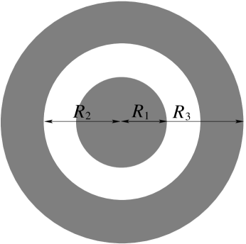
Figure 2: Distribution picture of $N_{1}$ eigenvalues in a disc and $N_{2}$ in the annulus.

In the following we will study the generalization corresponding to distributing $M$ holes in a circle centered around the origin. As discussed at the end of section 2 this leads to a droplet consisting of a black disc and an annulus (see Figure 2). The eigenvalues therefore get distributed in two disconnected droplets: a disc of radius $R_{1}=\sqrt{N_{1}}$ and an annular droplet of radii $R_{2}=\sqrt{N_{1}+M}$ and $R_{3}=\sqrt{N_{1}+N_{2}+M}$. Now, not only should one identify different near-BPS excitations associated to the three edges, but also be able to determine if a given semi-classical non-BPS excitations is localized either in the disc or in the annulus.

As we did for our first example, we analyze the action of $\partial_{Z}$ on the product of determinants

$$(\partial_{Z})^{i}_{j}\,{\cal O}^{(BPS)}_{LLM}=(\partial_{Z})^{i}_{j}\,\prod_{\alpha=1}^{M}\det(Z-\lambda_{\alpha})=M{(P)}^{i}_{j}\,{\cal O}^{(BPS)}_{LLM}\,.$$ (41)

The resulting $P$ matrix can be expressed in terms of the eigenvalues of the exterior droplet. To see this, it is convenient to use a matrix $\Lambda$ that diagonalizes $Z$

$$(P)^{i}_{j}\! \simeq \!\frac{1}{2\pi i}\sum_{k=1}^{N}(\Lambda)^{i}_{k}(\Lambda^{-1})^{k}_{j}\oint_{|\lambda|=r_{n}}\!\frac{d\lambda}{\lambda(z_{k}-\lambda)}{}$$ (42)

$$= \!\sum_{I/|z_{I}|>r}\frac{(\Lambda)^{i}_{I}(\Lambda^{-1})^{I}_{j}}{z_{I}}\,.$$

In particular, note that $PZ$ is a projector, satisfying $(PZ)^{2}=PZ$. Let us remark in passing that the action of $D_{0}$ on the product of determinants in (41) gives $M\,{\rm tr}(PZ)$ times the product of determinants and note that $M{\rm tr}(PZ)$ gives just a numerical factor $MN_{2}$. This is a reassuring result since one expects the BPS operator corresponding to a concentric eigenvalue distribution to have a definite number of $Z$ fields.

The presence of the operator $P$ suggests to write a general closed string excitation as

$$|\phi_{1},\ldots,\phi_{L}\rangle\leftrightarrow{\rm tr}(Y\phi_{1}(Z)Y\cdots Y\phi_{L}(Z))\prod_{\alpha=1}^{M}\det(Z-\lambda_{\alpha})\,,$$ (43)

where the possibilities for $\phi_{l}(Z)$ are

$$\phi_{l}(Z)=\left\{\begin{array}[]{ll}P^{n}&{\rm for\ }n\geq 1\\ Z_{P}^{n}\equiv Z^{n+1}P&{\rm for\ }n\geq 0\\ Z_{Q}^{n}\equiv Z^{n}-Z^{n+1}P&{\rm for\ }n\geq 0\end{array}\right..$$ (44)

Here the products $P^{n}$ can be thought of as negative powers of $Z$ with eigenvalues only belonging to (or projected onto) the annular droplet, while $Z_{P}^{n}$ and $Z_{Q}^{n}$ are thought of as positive powers of $Z$ projected onto the annulus and the disc respectively. The conclusion is that the appearance of the $P$ operator opens the possibility of occupying each site in the lattice with three different types of bosons.

The next step is to study the action of the one-loop dilatation operator (19) over the set of operators (43). However, the basis (44) is not the most appropriate one since states occupied by $Z_{P}^{n}$ and $Z_{Q}^{n}$ are not orthogonal. This may seem odd a first sight, since $Z_{P}^{n}$ is projected with $PZ$ and $Z_{Q}^{n}$ by its complement. Their interior product is

$$\langle Z_{P}^{n}|Z_{Q}^{n}\rangle\simeq\langle{\rm tr}(\overline{Z_{P}^{n}}Z_{Q}^{n})\rangle\,.$$ (45)

While $Z_{P}^{n}Z_{Q}^{n}$ is clearly zero, $\overline{Z_{P}^{n}}Z_{Q}^{n}$ is not. This is due to the matrix $Z$ being complex and $\Lambda$ being non-unitary in general. The set of orthogonal states we will consider is $\{|P^{n}\rangle,|Z_{P}^{0}\rangle,|n\rangle,|0\rangle,|Z_{Q}^{n}\rangle\}$ where

$$|0\rangle\equiv(N_{1}+M)|Z_{Q}^{0}\rangle+N_{1}|Z_{P}^{0}\rangle\,,$$ (46)

$$|n\rangle\equiv(N_{2}+M)|Z_{P}^{n}\rangle+N_{2}|Z_{Q}^{n}\rangle\quad{\rm for\ }n\geq 1\,,$$ (47)

The leading contribution to the action of $D_{1}$, when acting on the set discussed in the previous paragraph is again represented by a Hamiltonian of the form (24),

$$H=\lambda\sum_{l=1}^{L}(a_{l}-a_{l+1})^{\dagger}(a_{l}-a_{l+1})\,,$$ (48)

where the shift operators now act differently depending on the type of boson occupancy,

$$a|P^{n}\rangle\! = \!\sqrt{\nu_{1}+\gamma}\ |P^{n+1}\rangle\quad\quad{\rm if\ }n\geq 1\,,$$ (49)

$$a|Z_{P}^{0}\rangle\! = \!\sqrt{\nu_{1}+\gamma}|P\rangle\,,$$ (50)

$$a|0\rangle\! = \!0\,,$$ (51)

$$a|Z_{Q}\rangle\! = \!\sqrt{\frac{\nu_{1}\gamma(1+\gamma)}{(\nu_{1}+\gamma)(\nu_{2}+\gamma)}}|0\rangle-\sqrt{\frac{\nu_{1}^{2}\nu_{2}}{(\nu_{1}+\gamma)(\nu_{2}+\gamma)}}|Z_{P}^{0}\rangle\,,$$ (52)

$$a|1\rangle\! = \!\sqrt{\frac{\nu_{1}\nu_{2}(1+\gamma)}{(\nu_{1}+\gamma)(\nu_{2}+\gamma)}}|0\rangle+\sqrt{\frac{\gamma(1+\gamma)^{2}}{(\nu_{1}+\gamma)(\nu_{2}+\gamma)}}|Z_{P}^{0}\rangle\,,$$ (53)

$$a|Z_{Q}^{n}\rangle\! = \!\sqrt{\nu_{1}}\ |Z_{Q}^{n-1}\rangle\quad\quad\quad\quad{\rm if\ }n\geq 1\,,$$ (54)

$$a|n\rangle\! = \!\sqrt{1+\gamma}\ |{n-1}\rangle\quad\quad\ {\rm if\ }n\geq 1\,,$$ (55)

here $\gamma=\frac{M}{N}$, $\nu_{1}=\frac{N_{1}}{N}$ and $\nu_{2}=\frac{N_{2}}{N}$. As before, it is useful, for the semi-classical description, to define coherent states of the shift operator $a$. However, there is now no unique way of doing so. It is now possible to define coherent states involving no $|P^{n}\rangle$,

$$\!\!|z\rangle_{\rm I}\! = \!|0\rangle+\sqrt{\frac{\gamma(1+\gamma)}{(\nu_{1}+\gamma)(\nu_{2}+\gamma)}}\sum_{n=1}^{\infty}\left(\frac{z}{\sqrt{\nu_{1}}}\right)^{n}\!|Z_{Q}^{n}\rangle$$ (56)

$$+\sqrt{\frac{\nu_{1}\nu_{2}}{(\nu_{1}+\gamma)(\nu_{2}+\gamma)}}\sum_{n=1}^{\infty}\left(\frac{z}{\sqrt{1+\gamma}}\right)^{n}\!|n\rangle.$$

Alternatively, it is also possible to define coherent states involving no $|Z_{Q}^{n}\rangle$,

$$|z\rangle_{\rm II}=|0\rangle+\sqrt{\frac{\gamma(1+\gamma)}{\nu_{1}\nu_{2}}}|Z_{P}^{0}\rangle+\sqrt{\frac{\gamma(1+\gamma)}{\nu_{1}\nu_{2}}}\sum_{n=1}^{\infty}\left(\frac{z}{\sqrt{\nu_{1}+\gamma}}\right)^{-n}|P^{n}\rangle{}$$

$$\qquad\qquad+\sqrt{\frac{(\nu_{1}+\gamma)(\nu_{2}+\gamma)}{\nu_{1}\nu_{2}}}\sum_{n=1}^{\infty}\left(\frac{z}{\sqrt{1+\gamma}}\right)^{n}|n\rangle\ .$$ (57)

Both (56) and (57) satisfy $a|z\rangle=z|z\rangle$. Moreover (56) and(57) are normalizable in different complimentary domains,

$${}_{\rm I}\langle z|z\rangle_{\rm I}=1+\frac{\nu_{1}\nu_{2}}{(\nu_{1}+\gamma)(\nu_{2}+\gamma)}\sum_{n=1}^{\infty}\frac{|z|^{2n}}{\nu_{1}^{n}}+\frac{\gamma(1+\gamma)}{(\nu_{1}+\gamma)(\nu_{2}+\gamma)}\sum_{n=1}^{\infty}\frac{|z|^{2n}}{(1+\gamma)^{n}},$$ (58)

which is finite for $|z|<\nu_{1}$, the disc region, and

$${}_{\rm II}\langle z|z\rangle_{\rm II}=1+\frac{\gamma(1+\gamma)}{\nu_{1}\nu_{2}}\sum_{n=0}^{\infty}\frac{(\nu_{1}+\gamma)^{n}}{|z|^{2n}}+\frac{(\nu_{1}+\gamma)(\nu_{2}+\gamma)}{\nu_{1}\nu_{2}}\sum_{n=1}^{\infty}\frac{|z|^{2n}}{(1+\gamma)^{n}},$$ (59)

which is finite for $\nu_{1}+\gamma<|z|<1+\gamma$, the annulus region.

When using $|z\rangle_{\rm I}$ to compute the semi-classical action as done in (38)-(40), one finds (39) again. The only difference is in the function $V(z,\bar{z})$, which in the present case takes the form

$$V(z,\bar{z}) \!\!=\!\! \partial_{\bar{z}}\log(_{\rm I}\langle z|z\rangle_{\rm I}){}$$ (60)

$$\!\!=\!\! \frac{z}{\hat{R}_{3}^{2}-|z|^{2}}-\frac{z}{\hat{R}_{2}^{2}-|z|^{2}}+\frac{z}{\hat{R}_{1}^{2}-|z|^{2}}\,,$$

where ${\hat{R}}_{1}=\sqrt{\nu_{1}}$, ${\hat{R}}_{2}=\sqrt{\nu_{1}+\gamma}$ and ${\hat{R}}_{3}=\sqrt{1+\gamma}$. This is exactly the function $V(z,\bar{z})$ of a concentric droplet with three edges, for $|z|<{\hat{R}}_{1}$ (see (81))

Alternatively, when using $|z\rangle_{\rm II}$, a similar result is obtained for the semiclassical action, the function $V(z,\bar{z})$ in the (39) now being

$$V(z,\bar{z}) \!\!=\!\! \partial_{\bar{z}}\log(_{\rm II}\langle z|z\rangle_{\rm II}){}$$ (61)

$$\!\!=\!\! \frac{z}{{\hat{R}}_{3}^{2}-|z|^{2}}+\frac{z}{{\hat{R}}_{2}^{2}-|z|^{2}}-\frac{z}{{\hat{R}}_{1}^{2}-|z|^{2}}\,.$$

This is $V(z,\bar{z})$ as in (81) for ${\hat{R}}_{2}<|z|<{\hat{R}}_{3}$.

In conclusion, the two different coherent states $|z\rangle_{\rm I}$ and $|z\rangle_{\rm II}$ allow for two different large $L$ semiclassical limits. The first one valid for the disc $|z|<{\hat{R}}_{1}$ of the complex plane, while the second is valid for the annulus ${\hat{R}}_{2}<|z|<{\hat{R}}_{3}$. The two semi-classical actions so obtained for the bosonic lattice again coincide with the Polyakov action in the fast-string limit. Using $|z\rangle_{\rm I}$ leads to semiclassical strings stretching inside the disc and using $|z\rangle_{\rm II}$ to semiclassical strings within the black annulus.

4 Discussion

In this paper, we have derived in the large $N$ limit, the action of the one-loop dilatation operator on the set of gauge theory operators representing closed strings probing axially symmetric bubbling geometries whose corresponding droplets can have multiple edges and non-connected constituents. BMN-like limits were taken to extrapolate reliably the one-loop computations to strong ’t Hooft coupling and account for both geometrical and topological features of the bubbling geometries.

Concerning the topology of the SUGRA solutions, let us first remark that the gauge theory description was able to account for different sorts of BPS and near-BPS excitations that appear for multiple-edged droplets. The operators we found were in obvious correspondence with the dual string excitations traveling along null or almost null-geodesics (corresponding to the trajectories of BMN excitations) present on the droplet edges.

Motivated by [7], a large number of impurity fields $Y$ was inserted in the single trace operator corresponding to the closed string probe. In doing so, the gauge theory description reproduced the notion of LLM coordinates and was also able to reproduce some of the functions characterizing the bubbling metric. The novel characteristic for droplets with non-connected constituents was that different but complimentary semi-classical descriptions of the one-loop Hamiltonian were allowed. They precisely coincided with the actions of the possible semi-classical string solutions extending in each of the different disconnected components of the droplet with a fast-string limit imposed.

We specifically considered two bubbling configurations: the annulus, which is connected but has two edges, and the superposition of a disc and an annulus which is the simplest non-connected droplet.

Relying on the relation of $\frac{1}{2}$-BPS states of ${\cal N}=4$ SYM to matrix models [2, 14], we gave a prescription for the dual $\frac{1}{2}$-BPS operators to any arbitrary concentric droplet.

It has been previously seen that the action of the one-loop dilatation operator on the $SU(2)$ sub-sector operator can be reformulated in terms of the Hamiltonian of a bosonic lattice [8, 9]. In the first (annulus) example, we considered a single trace operator on top of $\det(Z)^{M}$. The Hamiltonian we obtained acts over a lattice whose sites can be occupied either by a positive or negative number of bosons. We explicitly solved the Hamiltonian spectrum for the case of large total boson occupation number, distinguishing the two possible cases of positive and negative occupations. In both cases the result was a BMN-like spectrum and the spectrum for positive (negative) occupation reproduced exactly the one obtained by quantizing a closed string traveling in the almost null-geodesic associated with the exterior (interior) edge of the annulus.

We remark that the axial symmetry of the droplets was essential for successfully computing the spectrum of the Hamiltonian. The axial symmetry entails a conserved total number of bosons. These eigenstates with definite number of bosons turn out to be solutions of a simple second order recurrent equation.

We also showed that the semi-classical sigma-model action for a lattice with a large number of sites coincides with a fast-string limit of the Polyakov action, when parameterized in such a way such that the angular momentum dual to the $R$-charge of the $Y$ fields is uniformly distributed along the string. This is in accordance with the bosonic lattice labeling of the probing single trace, since it uniformly accounts the $Y$ fields. In doing so, we were able to re-create the one-form $V_{a}$ of the LLM metric when restricted to the droplet plane $y=0$.

In the second (disc+annulus) example, the resulting Hamiltonian could again be expressed as acting on a bosonic lattice. In this case, the sites could be occupied by three different kinds of bosons. This was the gauge theory realization of the droplet having three edges. These corresponded to powers of the chiral complex $Z$ field projected either into the disc or into the annulus. It is significant to remark that the expression of the Hamiltonian is the same for all concentric cases, the difference being in the shift operators used. The action of the shift operators encodes the number of edges in the droplet and their radial distances to the origin. Moreover, for non-connected droplets, the set of coherent states of the shiftoperator is not unique. In the disc+annulus example, there were two possible types of coherent states $|z\rangle_{\rm I}$ in the domain $|z|<\hat{R}_{1}$, and $|z\rangle_{\rm II}$ in the domain $\hat{R}_{2}<|z|<\hat{R}_{3}$. The semi-classical descriptions derived from them coincided with the description of classical closed strings extended inside the disc or within the annulus of the droplet respectively.

Finally, it is interesting to mention that the isometry group $R\times SO(4)\times SO(4)$ of general LLM geometries is in fact the full bosonic component of $PSU(2|2)\times PSU(2|2)\ltimes R$. In the spin chain corresponding to $AdS_{5}\times S^{5}$, this is the residual symmetry of the ferromagnetic ground state. Short representations of the symmetry group extended to $PSU(2|2)\times PSU(2|2)\ltimes R^{3}$ give exact dispersion relations for elementary magnon excitations in the spin chain [22] as well as their bound states [23]. Open string solutions stretched between two points on the disc edge are interpreted as giant magnons [24] and magnon bound states [25], where the length of the string is related to the momentum carried by the magnon excitation. One can naturally ask if excitations with similar exact dispersion relation can exist in a general LLM background. Such solutions should again be an open string with ends at the edges of a general droplet. In this regard, we have found that there are semiclassical folded strings solutions in general LLM droplets, whose embedding is a straight line in the droplet with both folding points localized at edges. We could interpret our folded strings as a pair of generalized magnon bound states [25]. A crucial element in completing this argument is to construct scattering matrix between the generalization of elementary magnons, hence identifying the required pole for the bound states. We hope to return to this issues in near future.

Appendix

LLM geometries

In [3] Lin, Lunin and Maldacena worked out the regular 1/2 BPS solutions of type IIB supergravity with isometry group $R\times SO(4)\times SO(4)$. The geometric content of the solutions is given by the following metric.

$$ds^{2}=-h^{-2}(dt+V_{a}dx_{a})^{2}+h^{2}(dy^{2}+dx_{a}^{2})+ye^{G}d\Omega_{3}^{2}+ye^{-G}d{\tilde{\Omega}}_{3}^{2}\,,$$ (62)

where

$$h^{-2}=2y\cosh G\,,\quad\tanh G=2\rho(x_{1},x_{2},y)+1\,.$$ (63)

In general, the functions $V_{a}(x_{1},x_{2},y)$ and $\rho(x_{1},x_{2},y)$ are obtained by solving a linear differential equation with boundary conditions $\rho(x_{1},x_{2},0)$ specified on the two dimensional $y=0$ (droplet) plane. A smooth non-singular geometry requires $\rho(x_{1},x_{2},0)$ to take the values 0 or $-1$.

A concentric droplet with $K$ edges can be analytically solved, the functions $V_{a}$ and $\rho$ adopt the form

$$\!\!\!\!\!\rho(x_{1},x_{2},y)=\sum_{k=1}^{K}\frac{(-1)^{K-k}}{2}\!\left(\frac{r^{2}+y^{2}-R_{k}^{2}}{\sqrt{(r^{2}+y^{2}+R_{k}^{2})^{2}-4r^{2}R_{k}^{2}}}-1\right),$$ (64)

$$\!\!\!\!\!V_{\phi}(x_{1},x_{2},y)=\sum_{k=1}^{K}\frac{(-1)^{K-k+1}}{2}\!\left(\frac{r^{2}+y^{2}+R_{k}^{2}}{\sqrt{(r^{2}+y^{2}+R_{k}^{2})^{2}-4r^{2}R_{k}^{2}}}-1\right).$$ (65)

When the droplet is just the disc, the geometry is $AdS_{5}\times S^{5}$ and any compact droplet has $AdS_{5}\times S^{5}$ asymptotics. Notice that with a series of concentric annuli a concentric droplet with infinite black area can be constructed. In that case the resulting geometry possesses a different causal boundary [26].

Penrose limits and string spectra

The Penrose limits of LLM geometries corresponding to concentric droplets were computed in [27, 28], where the case of the annular droplets becoming thinner as the limit was taken. However, we are interested in the case where all the radii of the concentric domains are taken large while keeping their ratios fixed. The resulting plane wave geometries turn out to be the maximally supersymmetric plane-wane [29]. Nevertheless, it is important to keep track of the change of coordinates used in zooming a particular null geodesic of the LLM geometry in order to make a comparison among the string and gauge theory sides.

We consider the following change of coordinates in a generic LLM concentric droplet,

$$t=u\,,\qquad\qquad\qquad\phi=\pm\frac{v}{R_{i}}\,,$$ (66)

$$r=R_{i}+\frac{1}{2}(r_{1}^{2}-r_{2}^{2})\,,\quad y=r_{1}r_{2}\,,$$ (67)

where $R_{i}$ is the radius of any of the edges. The positive sign in (66) is chosen for the case where the edge separates an interior white region from an exterior black one. The negative sign is chosen for the opposite case. In both cases, taking all the $R_{i}$ to infinity, the resulting metric is the usual pp-wave

$$ds^{2}=-2dudv-(r_{1}^{2}+r_{2}^{2})du^{2}+d\vec{r}_{1}^{2}+d\vec{r}_{2}^{2}\,.$$ (68)

At this point we can just borrow the spectrum of $H_{lc}$ corresponding to a closed string in the background (68) [30],

$$H_{lc}=-p_{u}=\sum_{n}N_{n}\sqrt{1+\frac{n^{2}}{(\alpha^{\prime}p_{v})^{2}}}\,.$$ (69)

We can relate the charges $p_{u}$ and $p_{v}$ to the charges $E$ and $\hat{J}$ defined in coordinates that asymptotically tend to global $AdS_{5}\times S^{5}$ coordinates. Defining $\tilde{t}=t=u$ and $\tilde{\phi}=t+\phi=u\pm\frac{v}{R_{i}}$, we use

$$-p_{u}=i\partial_{u}=i(\partial_{\tilde{t}}+\partial_{\tilde{\phi}})=E-\hat{J}\,,$$ (70)

$$-p_{v}=i\partial_{v}=\pm\frac{i}{R_{i}}\partial_{\tilde{\phi}}=\mp\frac{\hat{J}}{R_{i}}\,,$$ (71)

to cast the spectrum (69) in the form,

$$E-\hat{J}=\sum_{n}N_{n}\sqrt{1+\frac{n^{2}R_{i}^{2}}{{\alpha^{\prime}}^{2}J^{2}}}=\sum_{n}N_{n}\sqrt{1+\frac{\pi R_{i}^{2}}{{\rm Area}(D)}\frac{8\pi^{2}n^{2}\lambda}{J^{2}}}\,,$$ (72)

where we have also used that Area$(D)=4\pi^{2}g_{s}N{\alpha^{\prime}}^{2}$.

Let us consider for instance the annular droplet. Choosing $R_{i}=R_{2}$ in (66)-(67), the Penrose limit zooms around the exterior edge. We use $\frac{\pi R_{2}^{2}}{{\rm Area}(D)}=1+\gamma$ and we let the angular momentum $\hat{J}$ take the value $J$. Expanding for $\frac{\lambda}{J^{2}}\ll 1$, we obtain

$$E\simeq J+2+(1+\gamma)\frac{8\pi^{2}n^{2}\lambda}{J^{2}}\,.$$ (73)

Similarly, the election $R_{i}=R_{1}$ zooms around the interior edge. In this case, $\frac{\pi R_{1}^{2}}{{\rm Area}(D)}=\gamma$ and we take the angular momentum $\hat{J}$ to be $-J$. Once again, expanding for $\frac{\lambda}{J^{2}}\ll 1$, we obtain

$$E\simeq-J+2+\gamma\frac{8\pi^{3}n^{2}\lambda}{J^{2}}\,,$$ (74)

where $\gamma$ is, as defined before, the ratio between area of the interior white disc and the area of the black annulus.

Semi-classical strings

Semiclassical strings in concentric LLM backgrounds have been previously studied in [31], [27], [32]. There, cases where the string was extended along $y$ were considered. We are interested instead in strings propagating in the $y=0$ section. More precisely, we will consider strings extended in any of the black regions of the LLM plane and also spinning along an angle $\eta$ of the transverse $S^{3}$. We will compare the description of these strings with large $J_{\eta}$ with a semiclassical description for the one-loop Hamiltonian with $L$ taken large. The index parameterizing the lattice hamiltonian counts uniformly the $Y$ fields of the single trace probing the BPS background operator. Then, a meaningful comparison with the string theory description can be done only fixing the parametrization of the worldsheet in a way such that $J_{\eta}$ is uniformly distributed along the string. This particular gauge fixing [33] in the Polyakov action for $AdS_{5}\times S^{5}$ written in LLM coordinates was originally done in [8] and more recently for a generic LLM geometry in [7], so we only quote the main result here. It is interesting to distinguish two possible situations. Firstly, some remarkable simplifications take place when restricting to static configurations in LLM coordinates, i.e. when $t=\tau$ and $r$ and $\phi$ only depending on $\sigma$. In that case, the resulting expression for the action is,

$$S=-\frac{L}{2\pi}\int d\tau\int_{0}^{2\pi}d\sigma\sqrt{1+\frac{1}{{\alpha^{\prime}}^{2}L^{2}}({r^{\prime}}^{2}+r^{2}{\phi^{\prime}}^{2})}\,,$$ (75)

Remarkably, all dependence on the LLM function $V_{\phi}(r,\phi)$ disappears. This holds even for the generic (non-axially symmetric) case. Thus, static solutions correspond to straight lines in the LLM droplet. Consider a folded string solution stretching between $R_{i}$ and $R_{i+1}$, so that its turning points move along light-like trajectories. This solution has the dispersion relation:

$$E-J=L\sqrt{1+\frac{(R_{i+1}-R_{i})^{2}}{\pi^{2}{\alpha^{\prime}}^{2}L^{2}}}=\sqrt{L^{2}+\frac{(R_{i+1}-R_{i})^{2}}{\pi^{2}{\alpha^{\prime}}^{2}}}\,.$$ (76)

The dispersion relation for the folded string in fact closely resembles the one for magnon bound states [25]. This can be made more transparent by introducing the normalized distance.

$$(\hat{R}_{i+1}-\hat{R_{i}})^{2}=\frac{\pi(R_{i+1}-R_{i})^{2}}{{\rm{Area}}(D)}\,,$$ (77)

where we have introduced the droplet area Area$(D)=4\pi^{2}g_{s}N{\alpha^{\prime}}^{2}=8\pi^{3}\lambda{\alpha^{\prime}}^{2}$. Using (77) in (76) we have

$$E-J=\sqrt{L^{2}+8\lambda(\hat{R}_{i+1}-\hat{R}_{i})^{2}}\,.$$ (78)

The folded string being a closed string solution should be thought of as a combination of two magnon bound states of equal charges but of opposite quasi-momentum. The magnon quasi-momentum can be identified with the distance stretched by the magnon in the droplet plane. In the case of a circular disc, this is given by $2\sin(p/2)$, whereas for the case of the annulus this is given by $(\hat{R}_{i+1}-\hat{R}_{i})$.

Considering a BMN-like expansion $\lambda/L^{2}\ll 1$ one has

$$E-J-L=\frac{4\lambda}{L}(\hat{R}_{i+1}-\hat{R}_{i})^{2}+...\,,$$ (79)

This precisely coincide with the weak coupling field theory result (35).

It is also interesting to consider the non-static configurations with a fast-string limit imposed [10, 11]. In this case the resulting action is

$$S=-\frac{L}{2\pi}\int d\tau\int_{0}^{2\pi}d\sigma\left(\dot{x}_{a}V_{a}+\frac{1}{2(\alpha^{\prime}L)^{2}}{x_{a}}^{\prime}{x_{a}}^{\prime}\right)\,,$$ (80)

In order to facilitate the comparison with field theory results, we define a normalized complex coordinate in the LLM plane $z=\sqrt{\frac{\pi}{{{\rm Area}(D)}}}(x_{1}+ix_{2})$. Writing the LLM functions in complex basis, for concentric droplets one has $\bar{z}V(z,\bar{z})=-V_{\phi}(x_{1},x_{2},0)$ with,

$$V(z,\bar{z})=\frac{z}{2|z|^{2}}\sum_{k=1}^{K}(-1)^{K-k}\left(\frac{|z|^{2}+{\hat{R}}_{k}^{2}}{||z|^{2}-{\hat{R}}_{k}^{2}|}-1\right)\,.$$ (81)

Here ${\hat{R}}_{k}$ are the normalized radii. Then, the Polyakov action in the fast-string limit adopts the form

$$S={L}\int d\tau\int_{0}^{1}d\sigma\left(\frac{i}{2}V\dot{\bar{z}}-\frac{i}{2}\bar{V}\dot{z}-\frac{\lambda}{L^{2}}|z^{\prime}|^{2}\right)\,,$$ (82)

This again precisely coincides with the coherent state action (39) defined for the Hamiltonian (24).

Some formulae

To study the action of the dilatation operator (19) over the single trace probing the background operator, it is necessary to consider $\partial_{Z}$ acting on positive and negative powers of $Z$ considered. For example,

$$(\partial_{Z})^{i}_{j}(Z^{n})^{k}_{l}=\sum_{a=1}^{n}(Z^{a-1})^{k}_{j}(Z^{n-a})^{i}_{l}\,,$$ (83)

$$(\partial_{Z})^{i}_{j}(Z^{-n})^{k}_{l}=-\sum_{a=1}^{n}(Z^{-a})^{k}_{j}(Z^{a-n-1})^{i}_{l}\,.$$ (84)

A careful inspection shows that, to the leading order in the large $N$ expansion, the relevant terms correspond to the case where an index of $\partial_{Z}$ is contracted with an index of $Z^{n}$. Even in that case, only one term of the sum contributes

$$(\partial_{Z})^{i}_{j}(Z^{n})^{j}_{l}=N(Z^{n-1})^{i}_{l}+\text{sub-leading}\,,$$ (85)

$$(\partial_{Z})^{i}_{j}(Z^{n})^{k}_{i}=N(Z^{n-1})^{k}_{j}+\text{sub-leading}\,.$$ (86)

The subleading terms in (19) give rise to multiple-traces probing the background operator and are suppressed in the large $N$ limit. The action of $\partial_{Z}$ is in all other cases always sub-leading.

In the case of three edges, we need the action of $\partial_{Z}$ over $P^{n}$ and $Z_{P}^{n}$ and $Z_{Q}^{n}$. Again, in the large $N$ limit the relevant contributions are

$$(\partial_{Z})^{i}_{j}(P^{n})^{j}_{l}=N_{1}(P^{n+1})^{i}_{l}+\text{sub-leading}\,,$$ (87)

$$(\partial_{Z})^{i}_{j}(P^{n})^{k}_{i}=N_{1}(P^{n+1})^{k}_{j}+\text{sub-leading}\,,$$ (88)

$$(\partial_{Z})^{i}_{j}(PZ)^{j}_{l}=N_{1}(P)^{i}_{l}+\text{sub-leading}\,,$$ (89)

$$(\partial_{Z})^{i}_{j}(PZ)^{k}_{i}=N_{1}(P)^{k}_{j}+\text{sub-leading}\,,$$ (90)

$$(\partial_{Z})^{i}_{j}(Z_{P}^{n})^{j}_{l}=N(Z_{P}^{n-1})^{i}_{l}+N_{2}(Z_{Q}^{n-1})^{i}_{l}+\text{sub-leading}\quad{\rm for\ }n\geq 1\,,$$ (91)

$$(\partial_{Z})^{i}_{j}(Z_{P}^{n})^{k}_{i}=N(Z_{P}^{n-1})^{k}_{j}+N_{2}(Z_{Q}^{n-1})^{k}_{j}+\text{sub-leading}\quad{\rm for\ }n\geq 1\,,$$ (92)

$$(\partial_{Z})^{i}_{j}(Z_{Q}^{n})^{j}_{l}=N_{1}(Z_{Q}^{n-1})^{i}_{l}+\text{sub-leading}\quad{\rm for\ }n\geq 1\,,$$ (93)

$$(\partial_{Z})^{i}_{j}(Z_{Q}^{n})^{k}_{i}=N_{1}(Z_{Q}^{n-1})^{k}_{j}+\text{sub-leading}\quad{\rm for\ }n\geq 1\,,$$ (94)

References

- [1] J. M. Maldacena, “The large N limit of superconformal field theories and supergravity,” Adv. Theor. Math. Phys. 2, 231 (1998) [arXiv:hep-th/9711200]. E. Witten, “Anti-de Sitter space and holography,” Adv. Theor. Math. Phys. 2, 253 (1998) [arXiv:hep-th/9802150]. S. S. Gubser, I. R. Klebanov and A. M. Polyakov, “Gauge theory correlators from non-critical string theory,” Phys. Lett. B 428, 105 (1998) [arXiv:hep-th/9802109].
- [2] D. Berenstein, “A toy model for the AdS/CFT correspondence,” JHEP 0407, 018 (2004) [arXiv:hep-th/0403110].
- [3] H. Lin, O. Lunin and J. Maldacena, “Bubbling AdS space and 1/2 BPS geometries,” JHEP 0410 (2004) 025 [arXiv:hep-th/0409174].
- [4] P. Horava and P. G. Shepard, “Topology changing transitions in bubbling geometries,” JHEP 0502, 063 (2005) [arXiv:hep-th/0502127].
- [5] D. Berenstein, “Large N BPS states and emergent quantum gravity,” JHEP 0601, 125 (2006) [arXiv:hep-th/0507203].
- [6] T. Brown, R. de Mello Koch, S. Ramgoolam and N. Toumbas, “Correlators, probabilities and topologies in N = 4 SYM,” arXiv:hep-th/0611290.
- [7] S. Vazquez, “Reconstructing 1/2 BPS space-time metrics from matrix models and spin chains,” arXiv:hep-th/0612014.
- [8] D. Berenstein, D. H. Correa and S. E. Vazquez, “Quantizing open spin chains with variable length: An example from giant gravitons,” Phys. Rev. Lett. 95, 191601 (2005) [arXiv:hep-th/0502172].
- [9] D. Berenstein, D. H. Correa and S. E. Vazquez, “A study of open strings ending on giant gravitons, spin chains and integrability,” JHEP 0609, 065 (2006) [arXiv:hep-th/0604123].
- [10] M. Kruczenski, “Spin chains and string theory,” Phys. Rev. Lett. 93, 161602 (2004) [arXiv:hep-th/0311203].
- [11] M. Kruczenski, A. V. Ryzhov and A. A. Tseytlin, “Large spin limit of AdS(5) x S**5 string theory and low energy expansion of ferromagnetic spin chains,” Nucl. Phys. B 692, 3 (2004) [arXiv:hep-th/0403120].
- [12] J. A. Minahan and K. Zarembo, ‘ ‘The Bethe-ansatz for N = 4 super Yang-Mills,” JHEP 0303 (2003) 013. [arXiv:hep-th/0212208].
- [13] D. Berenstein, J. M. Maldacena and H. Nastase, “Strings in flat space and pp waves from N = 4 super Yang Mills,” JHEP 0204, 013 (2002) [arXiv:hep-th/0202021].
- [14] S. Corley, A. Jevicki and S. Ramgoolam, “Exact correlators of giant gravitons from dual N = 4 SYM theory,” Adv. Theor. Math. Phys. 5, 809 (2002) [arXiv:hep-th/0111222].
- [15] A. Zabrodin, “Matrix models and growth processes: From viscous flows to the quantum Hall effect,” arXiv:hep-th/0412219.
- [16] D. Berenstein and R. Cotta, “A Monte-Carlo study of the AdS/CFT correspondence: an exploration of quantum gravity effects,” arXiv:hep-th/0702090.
- [17] N. Beisert, C. Kristjansen, J. Plefka, G. W. Semenoff and M. Staudacher, “BMN correlators and operator mixing in N = 4 super Yang-Mills theory,” Nucl. Phys. B 650, 125 (2003) [arXiv:hep-th/0208178].
- [18] D. H. Correa and G. A. Silva, “Dilatation operator and the super Yang-Mills duals of open strings on AdS giant gravitons,” JHEP 0611, 059 (2006) [arXiv:hep-th/0608128].
- [19] R. de Mello Koch, J. Smolic and M. Smolic, “Giant gravitons - with strings attached. II,” arXiv:hep-th/0701067.
- [20] S. S. Gubser, I. R. Klebanov and A. M. Polyakov, “A semi-classical limit of the gauge/string correspondence,” Nucl. Phys. B 636, 99 (2002) [arXiv:hep-th/0204051].
- [21] N. Beisert, J. A. Minahan, M. Staudacher and K. Zarembo, “Stringing spins and spinning strings,” JHEP 0309, 010 (2003) [arXiv:hep-th/0306139].
- [22] N. Beisert, “The su(2—2) dynamic S-matrix,” arXiv:hep-th/0511082.
- [23] H. Y. Chen, N. Dorey and K. Okamura, “The asymptotic spectrum of the N = 4 super Yang-Mills spin chain,” arXiv:hep-th/0610295.
- [24] D. M. Hofman and J. M. Maldacena, “Giant magnons,” J. Phys. A 39, 13095 (2006) [arXiv:hep-th/0604135].
- [25] N. Dorey, “Magnon bound states and the AdS/CFT correspondence,” J. Phys. A 39, 13119 (2006) [arXiv:hep-th/0604175].
- [26] A. E. Mosaffa and M. M. Sheikh-Jabbari, “On classification of the bubbling geometries,” JHEP 0604, 045 (2006) [arXiv:hep-th/0602270].
- [27] H. Ebrahim and A. E. Mosaffa, “Semiclassical string solutions on 1/2 BPS geometries,” JHEP 0501, 050 (2005) [arXiv:hep-th/0501072].
- [28] Y. Takayama and K. Yoshida, “Bubbling 1/2 BPS geometries and Penrose limits,” Phys. Rev. D 72, 066014 (2005) [arXiv:hep-th/0503057].
- [29] M. Blau, J. Figueroa-O’Farrill, C. Hull and G. Papadopoulos, “A new maximally supersymmetric background of IIB superstring theory,” JHEP 0201, 047 (2002) [arXiv:hep-th/0110242].
- [30] R. R. Metsaev, “Type IIB Green-Schwarz superstring in plane wave Ramond-Ramond background,” Nucl. Phys. B 625, 70 (2002) [arXiv:hep-th/0112044].
- [31] V. Filev and C. V. Johnson, “Operators with large quantum numbers, spinning strings, and giant gravitons,” Phys. Rev. D 71, 106007 (2005) [arXiv:hep-th/0411023].
- [32] M. Alishahiha, H. Ebrahim, B. Safarzadeh and M. M. Sheikh-Jabbari, “Semi-classical probe strings on giant gravitons backgrounds,” JHEP 0511, 005 (2005) [arXiv:hep-th/0509160].
- [33] G. Arutyunov and S. Frolov, “Integrable Hamiltonian for classical strings on AdS(5) x S**5,” JHEP 0502, 059 (2005) [arXiv:hep-th/0411089].