hep-th/0703066

The ODE/IM correspondence

Patrick Dorey¹, Clare Dunning² and Roberto Tateo³

¹Dept. of Mathematical Sciences, University of Durham,

Durham DH1 3LE, United Kingdom

²IMSAS, University of Kent, Canterbury, UK CT2 7NF, United Kingdom

³Dip. di Fisica Teorica and INFN, Università di Torino,

Via P. Giuria 1, 10125 Torino, Italy

E-mails:

p.e.dorey@durham.ac.uk, t.c.dunning@kent.ac.uk, tateo@to.infn.it

This article reviews a recently-discovered link between integrable quantum field theories and certain ordinary differential equations in the complex domain. Along the way, aspects of ${\cal P}{\cal T}$-symmetric quantum mechanics are discussed, and some elementary features of the six-vertex model and the Bethe ansatz are explained.

1 Introduction

Our aim in this article is to describe some links which are starting to emerge between two previously-separated areas of mathematical physics – the theory of integrable models in two dimensions, and the spectral analysis of ordinary differential equations.

The study of integrable lattice models has been an intriguing part of mathematical physics since Onsager’s solution of the two-dimensional Ising model. Lieb and Sutherland’s work on the six-vertex model showed that this was not an isolated phenomenon, and with Baxter’s work at the beginning of the 1970s the full richness of the field began to be appreciated by a wider community. Since that time interest in the subject has grown steadily, receiving a particular boost of late from the links which exist with integrable quantum field theories. Many different methods exist for the solution of these models, and a technique which will be very important in the following goes by the name of the ‘functional relations’ approach. The idea, initially put forward by Baxter, is to show that quantities of interest satisfy functional relations. When combined with suitable analyticity properties, these relations can be highly restrictive and often lead to exact formulae for quantities of physical interest.

In a parallel chain of development which also dates back at least to the early 1970s, Sibuya, Voros and others have shown that functional relations have an important rôle to play in a rather more classical area of mathematics, namely the theory of Stokes multipliers and spectral determinants for ordinary differential equations in the complex domain. However, it is only recently that the existence of a precise link – an ‘ODE/IM correspondence’ – between these two areas has been realised. The aim of these notes is to provide an elementary introduction to this connection and its background. For most of the time the focus will be on the simplest example, which connects second-order ordinary differential equations to integrable models associated with the Lie algebra $SU(2)$.

We begin, in the next section, with a short introduction to the types of spectral problems which will be relevant, mentioning in the process our third main theme, the intriguing reality properties of certain non-Hermitian spectral problems which arise in the study of ‘${\cal P}{\cal T}$-symmetric’ quantum mechanics. Integrable lattice models and their treatment via functional relations are introduced in section 3; we also discuss briefly the recent development of these ideas within quantum field theory. The differential equations side of the story is explained in section 4, after which the link with integrable models is made precise in section 5. Some applications and generalisations of the correspondence are outlined in section 6, and section 7 contains our conclusions. Various pieces of background material have been collected in the appendices, including an explanation of the algebraic Bethe ansatz in appendix A.

More on the ODE/IM correspondence can be found in references [1, 2, 3, 4, 5, 6, 7, 8, 9, 10, 11, 12, 13, 14, 15, 16, 17, 18, 19]. All of this work rests on earlier studies by, among others, Sibuya [20], Voros [21], and Bender et al [22, 23, 24] (on the ODE side) and by Baxter [25, 26], Klümper, Pearce and collaborators [27, 28], Fendley et al [29], and Bazhanov, Lukyanov and Zamolodchikov [30, 31, 32] on the integrable models side.

We have aimed to make this article accessible to readers with backgrounds in both the integrable models and the differential equations communities; for this reason, we have tried to keep the treatment relatively elementary. More details can be found in many places [20, 21, 33, 34].

Those readers primarily interested in ODEs may prefer to concentrate on section 2, briefly read sections 3.2, 3.9 and 3.10 to get a flavour of the integrable model picture, then move on to sections 4, 5 and 6, while those primarily interested in integrable models may like to look initially at sections 2, 3, 4 and then at 5.1, 5.2 and 5.6.

2 Prelude: three reality conjectures in ${\cal P}{\cal T}$-symmetric quantum mechanics

Spectral problems, some of a rather unconventional nature, will play a central rôle on the ‘differential equations’ side of our story. Rather than launch straight into technicalities, we shall warm up in this preliminary section by describing an intriguing class of problems much studied by Bender and collaborators and others in recent years. It all begins with a question posed by Bessis and Zinn-Justin, sometime near 1992:

Question 1: What does the spectrum of the Hamiltonian

$${\cal H}=p^{2}+ix^{3}$$ (2.1)

look like?

This is a cubic oscillator, with purely imaginary coupling $i$. (Strictly speaking, Bessis and Zinn-Justin, motivated by considerations of the Yang-Lee edge singularity [42, 43, 44], were initially interested in more general Hamiltonians of the form $p^{2}+x^{2}+igx^{3}$, from which the above problem emerged as a strong-coupling limit.) The corresponding Schrödinger equation is

$$-\frac{d^{2}}{dx^{2}}\psi(x)+ix^{3}\psi(x)=E\psi(x)$$ (2.2)

and we shall declare that the (possibly complex) number $E$ is in the spectrum if and only if, for that value of $E$, the equation has a solution $\psi(x)$ on the real axis which decays both at $x\to-\infty$ and at $x\to+\infty$, as illustrated in figure 1..

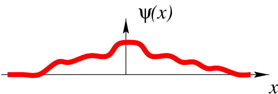
Figure 1: A wavefunction decaying at $x=\pm\infty$.

Notice that the differential equation forces the wavefunction $\psi(x)$ to be complex, even for real values of $x$ and $E$. And since the Hamiltonian is not (at least in any obvious way) Hermitian, the usual arguments to show that all of the eigenvalues must be real do not apply. Nevertheless, perturbative and numerical studies led Bessis and Zinn-Justin to the following claim:

Conjecture 1 [47]: The spectrum of ${\cal H}$ is real, and positive.

What might be behind this strange property? Bender and Boettcher [23] stressed the relevance of ${\cal P}{\cal T}$ symmetry. To be more precise, ‘${\cal P}$’, or parity, acts by sending $x$ to $-x$ and $p$ to $-p$ while ${\cal T}$, time reversal, sends $x$ to $x$, $p$ to $-p$ and $i$ to $-i$. Note that both ${\cal P}$ and ${\cal T}$ preserve the canonical commutation relation $[x,p]=i$ of quantum mechanics even if $x$ and $p$ are complex [24].

As shown in [24], ${\cal P}{\cal T}$ invariance implies that eigenvalues are either real, or appear in complex-conjugate pairs, much like the roots of a real polynomial. But, just as the typical real polynomial has many complex roots, on its own ${\cal P}{\cal T}$ invariance of the Hamiltonian does not guarantee reality. This is elegantly shown by the following generalisation of the Bessis-Zinn-Justin problem, proposed by Bender and Boettcher [23]:

Question 2: What is the spectrum of

$${\cal H}_{M}=p^{2}-(ix)^{2M}\qquad\quad\mbox{($M$ real, $>0$)}\,?$$ (2.3)

Later, it will turn out that the passage from question 1 to question 2 corresponds to a change in a parameter in a lattice model, or equivalently to a change of a quantum group deformation parameter in a Bethe ansatz system. But for now, the generalisation is appealing because it unites into a single family of eigenvalue problems both the $M=3/2$ case, for which we have the Bessis-Zinn-Justin conjecture, and the much more easily-understood $M=1$ case, the simple harmonic oscillator. Furthermore, for all $M$ the problem is ${\cal P}{\cal T}$-symmetric. The Schrödinger equation is now

$$-\frac{d^{2}}{dx^{2}}\psi(x)-(ix)^{2M}\psi(x)=E\psi(x)$$ (2.4)

and again we ask for those values of $E$ at which there is a solution along the real $x$-axis which decays at both plus and minus infinity. Two details need extra care: for non-integer values of $2M$, the ‘potential’ $-(ix)^{2M}$ is not single-valued; and when $M$ hits $2$, the naive definition of the eigenvalue problem runs into difficulties. The first problem is easily cured by adding a branch cut running up the positive imaginary $x$-axis. The second is more subtle, and its resolution more interesting; it will be discussed in greater detail in section 4 below.

For the moment, we shall agree to keep $M$ below $2$. Even so, there is an interesting surprise. Figure 2 is taken from [4] – it reproduces the results of [23]. Clearly, something strange occurs as $M$ decreases below $1$. Infinitely-many real eigenvalues pair off and become complex, and only finitely-many remain real. By the time $M$ has reached $0.75$, all but three have become complex, and as $M$ tends to $0.5$ the last real eigenvalue diverges to infinity. In fact, at $M{=}0.5$ the problem has no eigenvalues at all, as can be seen by shifting $ix$ to $ix-E$ and solving the resulting equation using an Airy function. For $M\geq 1$, numerical results combined with various pieces of analytical evidence indicated that the spectrum was entirely real, and positive, and so Bender and Boettcher generalised conjecture 1 to

Conjecture 2 [23]: The spectrum of ${\cal H}_{M}$ is real and positive for $M\geq 1$.

The ‘phase transition’ to infinitely-many complex eigenvalues at $M=1$ can be interpreted as a spontaneous breaking of ${\cal P}{\cal T}$ symmetry [23].

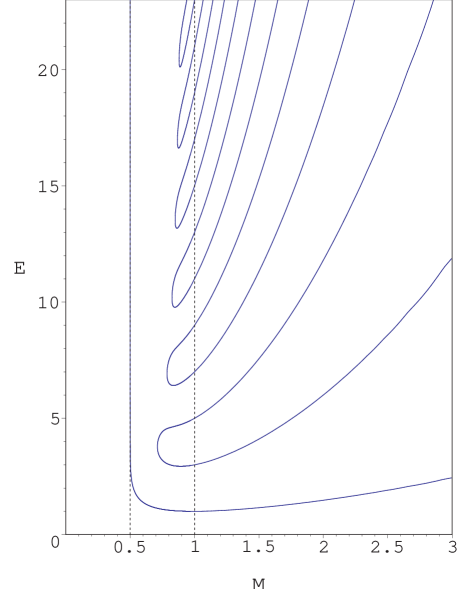
Figure 2: ${\cal H}_{M}=p^{2}-(ix)^{2M}$ : real eigenvalues as a function of $M$.

One further generalisation of the Bessis-Zinn-Justin conjecture will be relevant later. Consider

Question 3: What is the spectrum of

$${\cal H}_{M,l}=p^{2}-(ix)^{2M}+l(l{+}1)/x^{2}\qquad\mbox{($M$ and $l$ real, $M>0$)}\,?$$ (2.5)

This amounts to studying the effect of an angular-momentum-like term $l(l{+}1)x^{-2}$ on the Bender-Boettcher problem, and it was first investigated in [4]. Note that we continue to impose boundary conditions at $x=\pm\infty$, in the way stated just after equation (2.2) above. With the angular-momentum term included we need to specify how the wavefunction should be continued around the singularity at $x=0$; given the choice to place a branch cut on the positive-imaginary $x$ axis this continuation should be done through the lower half plane. (There will be much more discussion of boundary conditions later, so we won’t go into this detail any more for now.) Again, a combination of numerical and analytical work gave strong evidence for

Conjecture 3 [4]: The spectrum of ${\cal H}_{M,l}$ is real and positive for $M\geq 1$ and $|2l{+}1|<M{+}1$.

Although a small angular-momentum-like term does not have a significant effect while $M\geq 1$ and the eigenvalues all remain real, for $M<1$ it can make a remarkable difference to the way in which they become complex. Figure 3 shows the spectral plot for $l=-0.025$, and reveals a dramatic change from the earlier $l=0$ plot: the connectivity of the real eigenvalues has been reversed, so that while for $l=0$ the first and second excited states pair off, for $l=-0.025$ the first excited state is instead paired with the ground state, and so on up the spectrum. With this in mind, it may be hard to see how it is possible to pass between the sets of spectra depicted in figures 3 and 2 simply by varying the continuous parameter $l$ from $-0.025$ to zero. The mechanism should become clear by looking at the sample of intermediate pictures of figure 4.

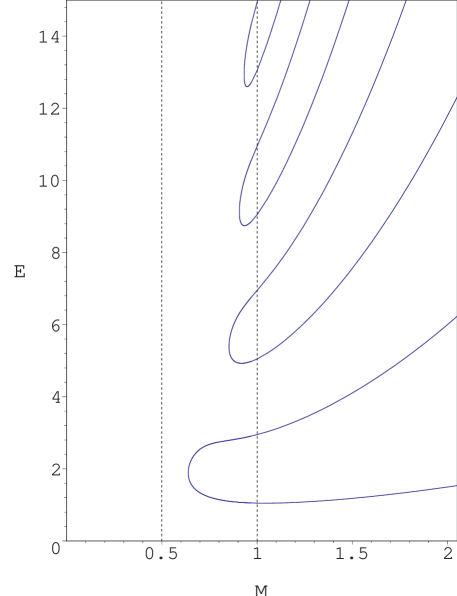
Figure 3: ${\cal H}_{M,l}=p^{2}-(ix)^{2M}+l(l{+}1)\,x^{-2}$ : real eigenvalues as a function of $M$ for $l=-0.025$, $l(l{+}1)=-0.024735$.

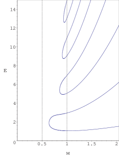
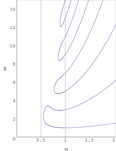
4a: $l=-0.025$

4b: $l=-0.005$

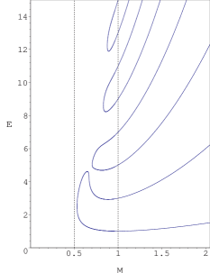
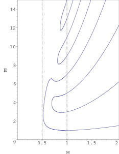
4c: $l=-0.0025$

4d: $l=-0.0015$

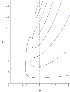
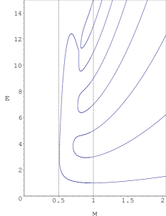
4e: $l=-0.001$

4f: $l=-0.0005$

Figure 4: Real eigenvalues of $p^{2}-(ix)^{2M}+l(l{+}1)/x^{2}$ as functions of $M$, for various values of $l$.

A final generalisation allows for an even richer phenomenology. Adding an inhomogeneous term $-\alpha(ix)^{M-1}$ to the potential for ${\cal H}_{M,l}$ gives a three-parameter family of problems:

$${\cal H}_{M,\alpha,l}=p^{2}-(ix)^{2M}-\alpha(ix)^{M-1}+l(l{+}1)/x^{2}.$$ (2.6)

Again, the first question to ask is whether the spectrum of ${\cal H}_{M,\alpha,l}$ is entirely real. Some general results will be described later in this review, but for now we illustrate the situation by giving some ‘experimental’ data for the case $M=3$. Special features of this particular case make it desirable to trade the parameter $l$ for $\rho:=\sqrt{3}(2l{+}1)$; this being understood, figure 5 shows, below the cusped line, the region of the $(\alpha,\rho)$ plane where all eigenvalues of ${\cal H}_{3,\alpha,l}$ are real. One last comment is worth making here: the alert reader might protest that substituting $M=3$ into (2.6) results in a Hamiltonian which is manifestly real, with a potential bounded from below, which should surely have an entirely real spectrum for all values of $\alpha$ and $l$ (or $\rho$). The question is a fair one, but it fails to take into account the fact that we have implicitly imposed boundary conditions which analytically continue those at $M=1$. This continuation takes $M$ past the value $2$ at which we already observed that there would be subtleties in defining the spectrum. We shall return to this point later.

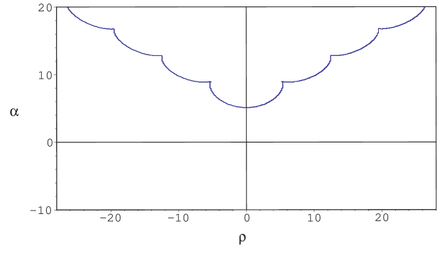
Figure 5: ${\cal H}_{3,\alpha,l}$ : region of unreality in the $(\alpha,\rho)$ plane, where $\rho=\sqrt{3}(2l{+}1)$.

Bender and Boettcher’s observation [23] has sparked a great deal of interest in reality properties in non-Hermitian quantum mechanics; a (small) sample of related work on the reality issue is provided by references [52, 53, 54, 55, 56, 57, 58, 59, 60, 61, 62, 63, 64, 65, 66, 67, 68, 69, 70, 71, 72, 73, 74, 75, 76, 77, 78, 79, 80, 81, 82, 83, 84, 85, 86, 87, 88, 89, 90, 91, 92, 93, 94, 95, 96, 97, 98, 99, 100, 101, 102, 103, 104, 105, 106, 107, 108, 109, 110, 111, 112]. In this already-long article, we won’t have space for any further discussion of non-Hermitian quantum mechanics in general; more on current issues in the field can be found in, for example, [41], the review article [113], the conference proceedings [114], and references therein. Instead we just remark that reality properties in ${\cal P}{\cal T}$-symmetric quantum mechanics of the sort described above have turned out to be surprisingly hard to establish by conventional means. An interesting byproduct of the ODE/IM correspondence has been a relatively elementary proof of conjectures 1, 2 and 3, and an understanding of many features of figure 5. We shall give this proof in section 6.2 below; it relies heavily on certain functional relations which had first made their appearance in a very different context: the theory of integrable lattice models. A rapid introduction to the background to this material is our next subject.

3 Integrable models and functional relations

In this section we shall introduce the integrable lattice models and quantum field theories that will be relevant later. One particular technique for their solution, the ‘functional relations’ approach, will be highlighted. We start with the lattice models, and then discuss what is known as the ‘continuum limit’ in preparation for the link with quantum-mechanical problems.

3.1 Generalities

Lattice models provide a way to understand the behaviours of magnets, and other substances, which exhibit a number of distinct ‘phases’ depending on the values taken by external parameters, such as the temperature. The simplest example is the Ising model, where a macroscopic magnet is modelled by a square lattice of microscopic ‘atoms’, each of which can exist in one of two states of magnetisation, up or down. By coupling nearest-neighbour atoms by an interaction which favours the lining-up of their magnetisations, a system is produced which captures the tendency of real magnets to exhibit an overall, macroscopic, magnetisation at low temperatures, which is then lost as the temperature is increased past some critical value. At this point, the model is said to undergo a ‘phase transition’, from an ‘ordered’ to a ‘disordered’ phase. The qualitative features of this behaviour can often be deduced from general arguments – the Peierls argument [115] is a good example – but for certain two-dimensional cases it turns out that much more can be said, and a number of important quantities can be calculated exactly as functions of the external parameters. Crudely speaking, these are the integrable lattice models, and the first example found was the two-dimensional Ising model, solved by Onsager in 1944 [116].

Much more can be said on this topic, but for the purposes of this review it is best now to move forward by two decades, and to describe the model which will be directly relevant to our subsequent story.

3.2 The six-vertex model and Bethe ansatz equations

We shall be interested in one particular set of integrable lattice models, called the ‘ice-type’ models, or, a little more prosaically, the six-vertex models. They were first solved in 1967, by Lieb [117] and Sutherland [118], and are among the simplest generalisations of the Ising model. Good places to look for further details are the book [33] by Baxter, and the short review [119] by McCoy.

The definition of the model begins with an $N\times N^{\prime}$ lattice, with periodic boundary conditions in both directions and, in order to avoid some annoying signs later on, $N/2$ even. Ultimately, we shall take a limit in which $N\to\infty$. On each horizontal or vertical link of the lattice, we place a spin $1$ or $2$, conveniently depicted by an arrow pointing either right or left (for the horizontal links) or up or down (for the vertical links), as in figure 6.

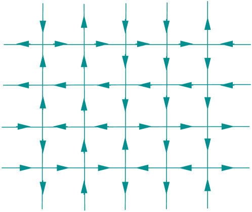
Figure 6: A typical configuration of spins for the six-vertex model.

In the ‘ice’ picture, each vertex represents an oxygen atom, and each link a bond between neighbouring atoms. Sitting on each bond is a hydrogen ion, lying near to one or the other end of the bond, according to the direction of the arrow. The ‘ice rule’ [121, 122] states that each oxygen atom should have exactly two hydrogen ions close to it, and two far away. Translated into the arrows, this implies that only those configurations that preserve the flux of arrows through each vertex are permitted. This means that there are six options for the spins around each site, or vertex, of the lattice (hence the alternative name ‘six-vertex’). For real ice, all allowed configurations are equally likely; but if we want to generalise slightly, then we can allow for differing probabilities for the different options. These overall probabilities are calculated in two steps. First, a number $W$, called a (local) Boltzmann weight, is assigned to each local possibility. If we further restrict ourselves to what is called the zero-field case, then the Boltzmann weights should be invariant under the simultaneous reversal of all arrows, and just three independent quantities need to be specified:

$$W\!\left[\mbox{$\rightarrow$\raisebox{6.45831pt}{$\uparrow$}\raisebox{-6.45831pt}{$\uparrow$}$\rightarrow$}\right]=W\!\left[\mbox{$\leftarrow$\raisebox{6.45831pt}{$\downarrow$}\raisebox{-6.45831pt}{$\downarrow$}$\leftarrow$}\right] = ~{}a~{};$$ (3.1)

$$W\!\left[\mbox{$\rightarrow$\raisebox{6.45831pt}{$\downarrow$}\raisebox{-6.45831pt}{$\downarrow$}$\rightarrow$}\right]=W\!\left[\mbox{$\leftarrow$\raisebox{6.45831pt}{$\uparrow$}\raisebox{-6.45831pt}{$\uparrow$}$\leftarrow$}\right] = ~{}b~{};$$ (3.2)

$$W\!\left[\mbox{$\rightarrow$\raisebox{6.45831pt}{$\uparrow$}\raisebox{-6.45831pt}{$\downarrow$}$\leftarrow$}\right]=W\!\left[\mbox{$\leftarrow$\raisebox{6.45831pt}{$\downarrow$}\raisebox{-6.45831pt}{$\uparrow$}$\rightarrow$}\right] = ~{}c~{}.$$ (3.3)

The relative probability of finding any given configuration is simply the product of the Boltzmann weights at the individual vertices. A first quantity to be calculated is the sum of these numbers over all possible configurations – the partition function, $Z$:

$$Z=\sum_{\{\sigma\}}\,\prod_{\rm sites}W\!\left[\mbox{$\,\cdot\,$\raisebox{6.45831pt}{$~{}\cdot\,$}\raisebox{-6.45831pt}{$\cdot\,$}$~{}\cdot\,$}\right]~{}.$$ (3.4)

One of the special features of integrable models is that quantities such as the partition function (or even better, the free energy per site, defined in equation (3.9) below) can be evaluated exactly, at least in the ‘thermodynamic limit’, where $N$ and $N^{\prime}$ both tend to infinity. The model under discussion turns out to be integrable for all values of $a$, $b$ and $c$. Their overall normalisation factors out trivially from all quantities, and it is convenient to parameterise the remaining two degrees of freedom using a pair of variables $\nu$ and $\eta$, called the spectral parameter and the anisotropy:

$$\quad a(\nu,\eta)=\sin(\eta+i\nu)~{},~{}~{}b(\nu,\eta)=\sin(\eta-i\nu)~{},{}~{}~{}c(\nu,\eta)=\sin(2\eta)~{}.\quad~{}~{}~{}$$ (3.5)

In calculations the anisotropy is usually held fixed, but it is useful to treat models with different values of the spectral parameter $\nu$ simultaneously. The weights can then be drawn as in figure 7.

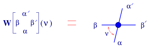
Figure 7: The local Boltzmann weights.

For those familiar with integrable quantum field theories, this picture might suggest a relationship between Boltzmann weights for integrable lattice models and S-matrix elements for integrable quantum field theories, with the spectral parameter of the Boltzmann weight proportional to the relative rapidity of two particles in the quantum field theory. We won’t explore this aspect much further here, but a nice discussion can be found in [123].

One popular tactic for the computation of the partition function employs the so-called transfer matrix, ${\mathbb{T}}$. Introduce multi-indices $\boldsymbol{\alpha}=(\alpha_{1},\alpha_{2}\dots\alpha_{N})$ and $\boldsymbol{\alpha}^{\prime}=(\alpha^{\prime}_{1},\alpha^{\prime}_{2}\dots\alpha^{\prime}_{N})$ and set

$${}~{}~{}{\mathbb{T}}^{\boldsymbol{\alpha}^{\prime}}_{\boldsymbol{\alpha}}(\nu){}~{}{}={}~{}{}\sum_{\{\beta_{i}\}}W\!\!\left[\mbox{$\beta_{1}$\raisebox{6.45831pt}{$\alpha^{\prime}_{1}$}\raisebox{-6.45831pt}{ $\alpha_{1}$}$\beta_{2}$}\right]\!\!(\nu)W\!\!\left[\mbox{$\beta_{2}$\raisebox{6.45831pt}{$\alpha^{\prime}_{2}$}\raisebox{-6.45831pt}{ $\alpha_{2}$}$\beta_{3}$}\right]\!\!(\nu)W\!\!\left[\mbox{$\beta_{3}$\raisebox{6.45831pt}{$\alpha^{\prime}_{3}$}\raisebox{-6.45831pt}{ $\alpha_{3}$}$\beta_{4}$}\right]\!\!(\nu)\dots W\!\!\left[\mbox{$\beta_{N}$\raisebox{6.45831pt}{$\alpha^{\prime}_{N}$}\raisebox{-6.45831pt}{ $\alpha_{N}$}$\beta_{1}$}\right]\!\!(\nu)\,.$$ (3.6)

A pictorial representation of ${\mathbb{T}}(\nu)$ is given in figure 8.

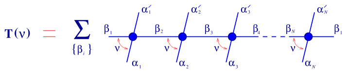
Figure 8: The transfer matrix.

The definition involves a sum over one set of horizontal links, and from the picture it is clear that the matrix indices of ${\mathbb{T}}$ correspond to the spin variables sitting on the vertical links. These can now be summed by matrix multiplication, with a final trace implementing the periodic boundary conditions in the vertical direction. Thus:

$$Z=\mbox{Trace}\left[{\mathbb{T}}^{N^{\prime}}\right]~{}.$$ (3.7)

Calculations can now continue via a diagonalisation of ${\mathbb{T}}$. Suppose that the first few eigenvalues, $t_{0}>t_{1}>\dots$ are known, with eigenvectors $\Psi^{(0)}$, $\Psi^{(1)}$, $\dots$ :

$$\sum_{\boldsymbol{\alpha}^{\prime}}{\mathbb{T}}^{\boldsymbol{\alpha}^{\prime}}_{\boldsymbol{\alpha}}\Psi^{(j)}_{\boldsymbol{\alpha}^{\prime}}=t_{j}\Psi^{(j)}_{\boldsymbol{\alpha}}~{}.$$ (3.8)

Then, for example, the free energy per site in the limit $N^{\prime}\to\infty$ can be obtained as

$$f=-{\textstyle\frac{1}{N\!N^{\prime}}}\log Z=-{\textstyle\frac{1}{N\!N^{\prime}}}\log\mbox{Trace}\left[{\mathbb{T}}^{N^{\prime}}\right]\sim-{\textstyle\frac{1}{N}}\log t_{0}~{}.$$ (3.9)

The eigenvalues $t_{0}$, $t_{1}$ …are functions of $\nu$ and $\eta$, and the remaining task is to find them. This appears to be a very tough problem – ${\mathbb{T}}$ is a $2^{N}\times 2^{N}$ matrix, and quickly becomes too large for even the most powerful computers to handle. It is necessary to exploit some of the special features of the model, and a popular technique for doing this goes by the name of the Bethe ansatz. There are two steps:

(i) Make a (well-informed) guess for a form for an eigenvector of ${\mathbb{T}}$, depending on a finite number $n$ of parameters $\nu_{1},\dots\nu_{n}$ (the ‘roots’).

(ii) Discover that this guess only works if the $\{\nu_{i}\}$ together solve a certain set of coupled equations (the ‘Bethe ansatz equations’).

Letting $n$ vary over a finite range, and for each $n$ taking the finite set of solutions to the corresponding Bethe ansatz equations, should then give totality of the eigenvectors of ${\mathbb{T}}$, or at least all those needed to capture the $N\to\infty$ limit of the system.

The justification of this procedure is an interesting story, or collection of stories, in its own right; in appendix A we outline one of the more elegant approaches, a technique called the algebraic Bethe ansatz.

For the six-vertex model, when the dust has settled the Bethe ansatz equations for the roots $\{\nu_{1}\dots\nu_{n}\}$ are

$$(-1)^{n}\prod_{j=1}^{n}\frac{\sinh(2i\eta-\nu_{k}+\nu_{j})}{\sinh(2i\eta-\nu_{j}+\nu_{k})}=-\frac{a^{N}\!(\nu_{k},\eta)}{b^{N}\!(\nu_{k},\eta)}~{}~{},\qquad k=1\dots n\,.$$ (3.10)

This is a set of $n$ equations for $n$ unknowns. There is no unique solution, but rather a discrete set. For each solution, an eigenvector $|\Psi\rangle$ of ${\mathbb{T}}$ can be constructed, with eigenvalue

$$t(\nu)=a^{N}\!(\nu,\eta)\prod_{j=1}^{n}g(\nu_{j}-\nu)+b^{N}\!(\nu,\eta)\prod_{j=1}^{n}g(\nu-\nu_{j})~{},$$ (3.11)

where $g(\nu):=a(\nu-i\eta,\eta)/b(\nu-i\eta,\eta)=-\sin(2\eta+i\nu)/\sin(i\nu)$ . To single out a given eigenvector and eigenvalue, supplementary conditions must be imposed on the roots. In particular, and this will be important later, the ground state eigenvalue $t_{0}(\nu)$ turns out to correspond, in the parameter region $0<\eta<\pi/2$, $\Re e(\nu)=0$, $-\eta<\Im m(\nu)<\eta$, to the Bethe ansatz solution with $n=N/2$ distinct real roots, packed as closely as possible and symmetrically placed about the origin (see for example [126, 33, 127]). This is depicted in figure 9.

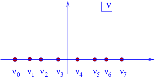
Figure 9: The $\nu_{i}$’s are real for the ground state.

3.3 Adding a twist

The periodic boundary conditions used above to define the transfer matrix can be modified in such a way that integrability is not spoilt (see for example [28, 128, 129]). This does not change the free energy per site in the thermodynamic limit, but it does modify some subleading effects.

The twist is introduced by modifying the local Boltzmann weights on one column, or seam, of the lattice, say the $N^{\rm th}$ (see figure 10).

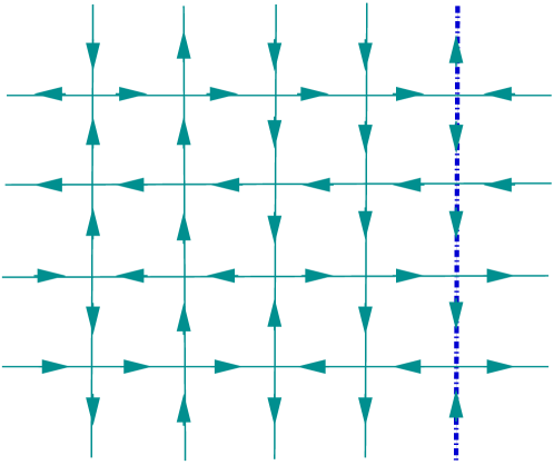
Figure 10: The twist is introduced by modifying the local Boltzmann weights on one column.

In the transfer matrix formulation the modification amounts to making the substitutions

$$W\!\left[\mbox{$\beta_{N}$\raisebox{6.45831pt}{$\alpha^{\prime}_{N}$}\raisebox{-6.45831pt}{ $\alpha_{N}$}$\rightarrow$}\right]\!(\nu)\Longrightarrow~{}e^{-i\phi}~{}W\!\left[\mbox{$\beta_{N}$\raisebox{6.45831pt}{$\alpha^{\prime}_{N}$}\raisebox{-6.45831pt}{ $\alpha_{N}$}$\rightarrow$}\right]\!(\nu)$$ (3.12)

and

$$W\!\left[\mbox{$\beta_{N}$\raisebox{6.45831pt}{$\alpha^{\prime}_{N}$}\raisebox{-6.45831pt}{ $\alpha_{N}$}$\leftarrow$}\right]\!(\nu)\Longrightarrow e^{i\phi}~{}W\!\left[\mbox{$\beta_{N}$\raisebox{6.45831pt}{$\alpha^{\prime}_{N}$}\raisebox{-6.45831pt}{ $\alpha_{N}$}$\leftarrow$}\right]\!(\nu)$$ (3.13)

in the initial definition (3.6) of ${\mathbb{T}}$. The algebraic Bethe ansatz works almost unchanged, with the result that the more general transfer matrix ${\mathbb{T}}(\nu,\phi)$ has eigenvalues given by

$$t(\nu,\phi)=e^{-i\phi}a^{N}\!(\nu,\eta)\prod_{j=1}^{n}g(\nu_{j}-\nu)+e^{i\phi}b^{N}\!(\nu,\eta)\prod_{j=1}^{n}g(\nu-\nu_{j})~{},$$ (3.14)

where the set of roots $\{\nu_{1}\dots\nu_{n}\}$ satisfy the modified Bethe ansatz equations

$$(-1)^{n}\prod_{j=1}^{n}\frac{\sinh(2i\eta-\nu_{k}+\nu_{j})}{\sinh(2i\eta-\nu_{j}+\nu_{k})}=-e^{-2i\phi}\frac{a^{N}\!(\nu_{k},\eta)}{b^{N}\!(\nu_{k},\eta)}~{}~{},\qquad k=1\dots n\,.$$ (3.15)

3.4 The $XXZ$ model

There is a well-known connection between classical two dimensional lattice models and quantum spin chains. The six-vertex model is related to the (spin $1/2$) $XXZ$ spin chain, a one-dimensional system of $N$ lattice sites with a spin variable taking the value $1$ or $2$ at each site, with each spin interacting only with its neighbours. The Hamiltonian is

$$H_{XXZ}=-\frac{1}{2}\sum_{j=1}^{N}\left(\sigma_{j}^{x}\sigma_{j+1}^{x}+\sigma_{j}^{y}\sigma_{j+1}^{y}-\cos 2\eta\,\sigma_{j}^{z}\sigma_{j+1}^{z}\right)~{},$$ (3.16)

where $\sigma_{j}^{\alpha}$ represents a Pauli matrix,

$$\sigma^{x}_{j}=\Big{(}\!\begin{array}[]{rr}0&1\\[-1.0pt] 1&0\end{array}\!\Big{)}\,,\quad\sigma^{y}_{j}=\Big{(}\!\begin{array}[]{rr}0&-i\\[-1.0pt] i&0\end{array}\!\Big{)}\,,\quad\sigma^{z}_{j}=\Big{(}\!\begin{array}[]{rr}1&0\\[-1.0pt] 0&-1\end{array}\!\Big{)}\,,$$ (3.17)

acting on the spin on the $j^{\rm th}$ lattice site. This model is sometimes also referred to as the Heisenberg-Ising chain, or the spin $1/2$ anisotropic Heisenberg chain. The six-vertex twist can be implemented by imposing twisted boundary conditions of the form

$$\sigma_{N+1}^{z}=\sigma_{1}^{z}\quad,\quad\sigma_{N+1}^{x}\pm i\sigma_{N+1}^{y}=e^{\pm i2\phi}\bigl{(}\sigma_{1}^{x}\pm i\sigma_{1}^{y}\bigr{)}\,.$$ (3.18)

From these definitions it is not obvious that the six-vertex and $XXZ$ models should be related. However it was noticed in the first work on the six-vertex model [117, 118] that its transfer matrix eigenvectors coincided with those of $H_{XXZ}$ , previously studied in great detail by Yang and Yang [130]. The initial identification rested on a coincidence of Bethe ansatz equations, and was given a more direct explanation when Baxter [131] showed that the six-vertex transfer matrix ${\mathbb{T}}$ and the Hamiltonian of the spin chain are directly connected through the relation

$$H_{XXZ}=-i\sin 2\eta\,\frac{d}{d\nu}\ln{\mathbb{T}}(\nu)\Bigr{|}_{\nu=-i\eta}-\frac{1}{2}\cos 2\eta\ {\mathbb{I}}^{\otimes N}\,.$$ (3.19)

Consequently, if we are able to determine the eigenvalues $t_{0},t_{1}\dots$ of the transfer matrix we gain, for free, information on the spectrum of the $XXZ$ model.

We shall return to a description of the six-vertex spectrum motivated by this connection with the $XXZ$ model shortly, but for now we note that for all values of the twist parameter, the Hamiltonian (3.16) commutes with the total spin operator $S^{z}=\sum_{i=1}^{N}\sigma_{i}^{z}/2$. Therefore the spectrum splits into disjoint sectors labelled by the spin $m=0,1,2\dots~{}$; and the true ground state lies in the $m=0$ sector. In the six-vertex model the $XXZ$ spin sectors correspond to taking the number of Bethe roots $n$ different from the ground state value of $n=N/2$. The relation between the number of Bethe roots and the $XXZ$ spin is $n=N/2-m$.

3.5 Baxter’s TQ relation

So much, for now, for the Bethe ansatz. There is a particularly neat reformulation of the final result, discovered by Baxter, that leads to an alternative way to solve the model. The first ingredient is the fact that the transfer matrices at different values of the spectral parameter $\nu$ commute:

$$[{\mathbb{T}}(\nu),{\mathbb{T}}(\nu^{\prime})]=0\,.$$ (3.20)

(The (standard) proof of this fact is given in appendix A.) Therefore, the transfer matrices ${\mathbb{T}}(\nu)$ can be simultaneously diagonalised, with eigenvectors which are independent of $\nu$. This allows us to focus on the individual eigenvalues $t_{0}(\nu)$, $t_{1}(\nu)$, … as functions of $\nu$. From the explicit form of the Boltzmann weights and the claim that the eigenvectors are $\nu$-independent, these functions are entire, and $i\pi$-periodic.

The second ingredient is the claim that, for each eigenvalue function $t(\nu)$, there exists an auxiliary function $q(\nu)$, also entire and (at least for the ground state) $i\pi$-periodic, such that

$$t(\nu)q(\nu)=e^{-i\phi}a^{N}\!(\nu,\eta)q(\nu+2i\eta)+e^{i\phi}b^{N}\!(\nu,\eta)q(\nu-2i\eta)\,.$$ (3.21)

We shall call this the TQ relation, though this phrase should really be reserved for the corresponding matricial equation, involving ${\mathbb{T}}(\nu)$ and another matrix ${\mathbb{Q}}(\nu)$, from which the above can be extracted when acting on eigenvectors. At first sight, it is not clear why this should encode the whole elaborate structure of the Bethe ansatz equations – instead of one unknown function $t(\nu)$, we now have two, and all we know about them is that they enjoy the curious relationship given by (3.21). But in fact this equation, combined with the simultaneous entirety of $t(\nu)$ and $q(\nu)$, imposes constraints on $t(\nu)$ which are so strong that there is no need to impose the BAE as a supplementary set of conditions. (Going further, Baxter was able to establish the TQ relation by an independent argument, thereby finding an alternative treatment of the six-vertex model which avoided the explicit construction of eigenvectors. He then generalised this approach to the previously unsolved eight-vertex model, but we shall not elaborate this aspect any further here.)

The BAE are extracted from (3.21) as follows. Suppose, anticipating the final result in the notation, that the zeros of $q(\nu)$ are at $\nu_{1}$, …$\nu_{n}$ . Given that $q(\nu)$ is $i\pi$-periodic, it can – up to an irrelevant overall normalisation – be written as a product over these zeros as

$$q(\nu)=\prod^{n}_{l=1}\sinh(\nu-\nu_{l})~{}.$$ (3.22)

From (3.21), $t(\nu)$ is fixed by $q(\nu)$, and from (3.22), $q(\nu)$ is fixed by the set $\{\nu_{i}\}$. To determine the $\{\nu_{i}\}$, set $\nu=\nu_{i}$ in (3.21). On the left-hand side we then have $t(\nu_{i})$, which is nonsingular since $t(\nu)$ is entire, multiplied by $q(\nu_{i})$ which is zero by (3.22). Thus the left-hand side vanishes, and rearranging we have

$$\frac{q(\nu_{i}-2i\eta)}{q(\nu_{i}+2i\eta)}=-e^{-2i\phi}\frac{a^{N}\!(\nu_{i},\eta)}{b^{N}\!(\nu_{i},\eta)}~{}~{}$$ (3.23)

or, using (3.22) one more time,

$$(-1)^{n}\prod^{n}_{l=1}\frac{\sinh(2i\eta-\nu_{i}+\nu_{l})}{\sinh(2i\eta-\nu_{l}+\nu_{i})}=-e^{-2i\phi}\frac{a^{N}\!(\nu_{i},\eta)}{b^{N}\!(\nu_{i},\eta)}~{}~{},\qquad i=1\dots n~{}.$$ (3.24)

These are exactly the Bethe ansatz equations (3.15) for the problem, with the $\nu_{i}$ the roots. The expression for $t(\nu)$ implied by (3.21) then matches the formula (3.14), as would have been found from a direct application of the Bethe ansatz.

3.6 The quantum Wronskian

In this review, the TQ relation will be our main tool in making the link with the theory of ordinary differential equations. However, there are other sets of functional equations associated with the six-vertex model which can be equally important. In principle these can all be obtained first as operator equations (see for example [26, 33, 31, 132]), and then turned into functional relations by specialising to individual eigenvectors. However a full discussion of this would take us too far afield, so instead we shall profit from the fact that we have already obtained the TQ relation from the lattice model, and give some indications as to why these further properties should hold.

We continue to consider the model with general (non-zero) twist, and discuss an important consequence of the identity (A.48):

$$t_{0}(\nu,\phi)=t_{0}(\nu,-\phi)\equiv t_{0}(\nu,|\phi|)~{},$$ (3.25)

where $t_{0}$ is the ground state eigenvalue of ${\mathbb{T}}(\nu,\phi)$ (with $N/2$ even) and $\phi$ is the twist parameter. In view of (3.25), the following two TQ relations hold simultaneously:

$$\!\!\!\!\!\!\!t_{0}(\nu,|\phi|)\,q_{0}(\nu,\phi) = a^{N}\!(\nu,\eta)e^{-i\phi}q_{0}(\nu+2i\eta,\phi)+b^{N}\!(\nu,\eta)e^{i\phi}q_{0}(\nu-2i\eta,\phi)\,;$$ (3.26)

$$\!\!\!\!\!\!\!t_{0}(\nu,|\phi|)\,q_{0}(\nu,-\phi) = a^{N}\!(\nu,\eta)e^{i\phi}q_{0}(\nu+2i\eta,-\phi)+b^{N}\!(\nu,\eta)e^{-i\phi}q_{0}(\nu-2i\eta,-\phi)$$ (3.27)

where $q_{0}$ is the corresponding ground state eigenvalue of the corresponding matrix ${\mathbb{Q}}(\nu,\phi)$. As equations for $q$, these only differ in the way that the twist factors $e^{\pm i\phi}$ appear, and even this difference can be eliminated by defining

$$\widetilde{q}_{0}(\nu,\phi):=e^{-\nu\phi/(2\eta)}q_{0}(\nu,\phi)$$ (3.28)

so that

$$\quad t_{0}(\nu,|\phi|)\,\widetilde{q}_{0}(\nu,\phi) = a^{N}\!(\nu,\eta)\widetilde{q}_{0}(\nu+2i\eta,\phi)+b^{N}\!(\nu,\eta)\widetilde{q}_{0}(\nu-2i\eta,\phi)\,;$$ (3.29)

$$\quad t_{0}(\nu,|\phi|)\,\widetilde{q}_{0}(\nu,-\phi) = a^{N}\!(\nu,\eta)\widetilde{q}_{0}(\nu+2i\eta,-\phi)+b^{N}\!(\nu,\eta)\widetilde{q}_{0}(\nu-2i\eta,-\phi)\,.$$ (3.30)

Thus $\widetilde{q}_{0}(\nu,\phi)$ and $\widetilde{q}_{0}(\nu,-\phi)$ both solve the single functional equation

$$t_{0}(\nu,|\phi|)\,\widetilde{q}(\nu)=a^{N}\!(\nu,\eta)\widetilde{q}(\nu+2i\eta)+b^{N}\!(\nu,\eta)\widetilde{q}(\nu-2i\eta)\,.$$ (3.31)

This is a finite-difference analogue of a second-order ordinary differential equation, and so it should have two linearly independent solutions; equations (3.29) and (3.30) confirm that this is indeed the case. The quasi-periodicity in $\nu$ induced by the definition (3.28), combined with the periodicity of the ‘potential’ $t_{0}$, means that $\widetilde{q}_{0}(\nu,\phi)$ and $\widetilde{q}_{0}(\nu,-\phi)$ can be interpreted as the two Bloch-wave solutions to (3.31) [31, 133]. Just as in the continuum case, given two solutions to a single second-order equation it is natural to construct their Wronskian. To this end, we can multiply (3.29) by $\widetilde{q}_{0}(\nu,-\phi)$ and (3.30) by $\widetilde{q}_{0}(\nu,\phi)$, subtract and regroup terms by defining

$$\Delta(\nu):=\widetilde{q}_{0}(\nu{+}i\eta,-\phi)\widetilde{q}_{0}(\nu{-}i\eta,\phi)-\widetilde{q}_{0}(\nu{+}i\eta,\phi)\widetilde{q}_{0}(\nu{-}i\eta,-\phi)$$ (3.32)

to find

$$0=a^{N}\!(\nu,\eta)\Delta(\nu{+}i\eta)-b^{N}\!(\nu,\eta)\Delta(\nu{-}i\eta)\,.$$ (3.33)

Recalling from (3.5) the definitions $a(\nu,\eta)=\sin(\eta+i\nu)$, $b(\nu,\eta)=\sin(\eta-i\nu)$, and the fact that $N$ is even, (3.33) implies that the function ${\cal W}(\nu):=\Delta(\nu)/\sinh^{N}(\nu)$ is periodic with period $P=2i\eta$. However, from (3.22) and (3.28), we see that ${\cal W}(\nu)$ also has the period $P^{\prime}=2i\pi$. For $P^{\prime}/P=\eta/\pi$ irrational, ${\cal W}(\nu)$ must therefore be constant; by continuity in $\eta$, ${\cal W}(\nu)$ is constant for all values of $\eta$.

Evaluating ${\cal W}$ at $\nu\rightarrow\infty$ gives an identity, the finite-lattice version of the quantum Wronskian relation discussed by Bazhanov, Lukyanov and Zamolodchikov in [31]. Re-expressed in terms of $q_{0}(\nu,\phi)$ it reads

$$\ e^{-i\phi}q_{0}(\nu{+}i\eta,\phi)q_{0}(\nu{-}i\eta,-\phi)-e^{i\phi}q_{0}(\nu{+}i\eta,-\phi)q_{0}(\nu{-}i\eta,\phi)=-2i\sin(\phi)\,\sinh^{N}(\nu).$$ (3.34)

In deriving this result we have only treated the ground state eigenvalues of ${\mathbb{T}}$ and ${\mathbb{Q}}$, and we have also assumed that the twist $\phi$ is non-zero. If these restrictions are dropped, a number of important subtleties arise, particularly in the so-called ‘root of unity’ cases when $P^{\prime}/P$ is rational. For more extensive discussions which address some of these issues, see, for example, [134] and [135, 136].

3.7 The fusion hierarchy and its truncation

A further functional equation results if we multiply the simultaneous TQ relations (3.29) and (3.30) by $\widetilde{q}_{0}(\nu{-}2i\eta,-\phi)$ and $\widetilde{q}_{0}(\nu{-}2i\eta,\phi)$, respectively, and subtract. We then obtain not the quantum Wronskian, but instead an alternative expression for $t_{0}$ in terms of ${\widetilde{q}}_{0}$ :

$$\!\!\!\!\!\!\!\!\!\!\!t_{0}(\nu,|\phi|) = a^{N}\!(\nu,\eta)\,{\widetilde{q}_{0}(\nu{+}2i\eta,-\phi)\widetilde{q}_{0}(\nu{-}2i\eta,\phi)-\widetilde{q}_{0}(\nu{+}2i\eta,\phi)\widetilde{q}_{0}(\nu{-}2i\eta,-\phi)\over\widetilde{q}_{0}(\nu,\phi)\widetilde{q}_{0}(\nu{-}2i\eta,-\phi)-\widetilde{q}_{0}(\nu,-\phi)\widetilde{q}_{0}(\nu{-}2i\eta,\phi)}$$ (3.35)

$$= \frac{-1}{2i\sin\phi}\,\Bigl{(}\widetilde{q}_{0}(\nu{+}2i\eta,-\phi)\widetilde{q}_{0}(\nu{-}2i\eta,\phi)-\widetilde{q}_{0}(\nu{+}2i\eta,\phi)\widetilde{q}_{0}(\nu{-}2i\eta,-\phi)\Bigr{)}$$

using the previously-obtained formula for the quantum Wronskian for the last equality. This is a sign that the quantum Wronskian fits into a hierarchy of relations which we now describe. It is convenient to change the normalisations slightly. Defining

$$\vec{q}^{\,(k)}:={1\over\sqrt{-2i\sin\phi}}\Big{(}e^{-ik\phi/2}q_{0}(\nu{-}ik\,\widetilde{\eta},\phi),e^{ik\phi/2}q_{0}(\nu{-}ik\,\widetilde{\eta},-\phi)\Big{)}^{T}$$ (3.36)

with $\widetilde{\eta}=-\eta{+}\pi/2$ and

$${\cal W}[k,-k](\nu):=\det(\vec{q}^{\,(k)},\vec{q}^{\,(-k)})=\left|\left|\begin{array}[]{cc}(q^{(k)})_{1}&(q^{(-k)})_{1}\\ (q^{(k)})_{2}&(q^{(-k)})_{2}\end{array}\right|\right|~{},$$ (3.37)

we set

$$t^{(k/2)}(\nu):={\cal W}[k+1,-k-1](\nu)~{},~{}~{}~{}k=-1,0,1,2,3\dots~{}.$$ (3.38)

Then $t^{(-1/2)}(\nu)=0$, and (3.34) and (3.35) imply

$$t^{(0)}(\nu)=[i\cosh(\nu)]^{N}~{},\quad t^{(1/2)}(\nu)=t_{0}(\nu)\,.$$ (3.39)

We can then use the following Plücker-type relation

$$\quad\det(\vec{a}_{0},\vec{a}_{1})\det(\vec{b}_{0},\vec{b}_{1})=\det(\vec{b}_{0},\vec{a}_{1})\det(\vec{a}_{0},\vec{b}_{1})+\det(\vec{b}_{1},\vec{a}_{1})\det(\vec{b}_{0},\vec{a}_{0})$$ (3.40)

and the property

$${\cal W}[k+a,-k+a](\nu)={\cal W}[k,-k](\nu-ia\widetilde{\eta})$$ (3.41)

to show that

$$t^{(m)}(\nu-i\widetilde{\eta})t^{(m)}(\nu+i\widetilde{\eta})=$$

$$\qquad t^{(0)}(\nu-i(2m{+}1)\widetilde{\eta})t^{(0)}(\nu+i(2m{+}1)\widetilde{\eta})+t^{(m{-}1/2)}(\nu)t^{(m{+}1/2)}(\nu)~{},$$ (3.42)

where the index $m$ takes the half-integer values $1/2$, $1$, $3/2$, $\dots$ . Another set of relations among the functions $t^{(m)}(\nu)$ is also a simple consequence of the identity (3.40):

$$t^{(1/2)}(\nu)t^{(m)}(\nu-i(2m{+}1)\widetilde{\eta})=$$

$$t^{(0)}(\nu-i\widetilde{\eta})t^{(m{+}1/2)}(\nu-i2m\widetilde{\eta})+t^{(0)}(\nu+i\widetilde{\eta})t^{(m{-}1/2)}(\nu-i(2m{+}2)\widetilde{\eta})~{}.$$ (3.43)

The sets of functional relations (3.42) and (3.43) are called fusion hierarchies [137, 138, 139, 140, 31]. The name comes from the fact that they can also be obtained by a process known as ‘fusion’ of the basic transfer matrix ${\mathbb{T}}$, without introducing the auxiliary function $q(\nu)$ [141].

An important phenomenon occurs at rational values of $\eta/\pi$, known as truncation of the fusion hierarchy. Here we shall just mention the case $\eta={\pi M\over 2M+2}$ ($\widetilde{\eta}={\pi\over 2M+2}$) with $2M\in{\mathbb{Z}}^{+}$ and $\phi={\pi\over 2M+2}$. Due to the $i\pi$ periodicity of $q(\nu)$ we have

$$t^{(M+1/2)}(\nu)=0$$ (3.44)

and also

$$\begin{array}[]{ccc}\vec{q}^{(2M+1)}&=&{-i\over\sqrt{-2i\sin\phi}}\Big{(}e^{{\textstyle\frac{i\pi}{4M+4}}}q_{0}(\nu{+}{\textstyle\frac{i\pi}{2M+2}},\phi),-e^{-{\textstyle\frac{i\pi}{4M+4}}}q_{0}(\nu{+}{\textstyle\frac{i\pi}{2M+2}},-\phi)\Big{)}^{T}~{};\\ \ \ \vec{q}^{(-2M-1)}&=&{i\over\sqrt{-2i\sin\phi}}\Big{(}e^{-{\textstyle\frac{i\pi}{4M+4}}}q_{0}(\nu{-}{\textstyle\frac{i\pi}{2M+2}},\phi),-e^{{\textstyle\frac{i\pi}{4M+4}}}q_{0}(\nu{-}{\textstyle\frac{i\pi}{2M+2}},-\phi)\Big{)}^{T}~{},\end{array}$$ (3.45)

which on comparing with

$$\begin{array}[]{ccc}\vec{q}^{(1)}&=&{1\over\sqrt{-2i\sin\phi}}\Big{(}e^{-{\textstyle\frac{i\pi}{4M+4}}}q_{0}(\nu{-}{\textstyle\frac{i\pi}{2M+2}},\phi),e^{{\textstyle\frac{i\pi}{4M+4}}}q_{0}(\nu{-}{\textstyle\frac{i\pi}{2M+2}},-\phi)\Big{)}^{T}~{};\\ \ \ \vec{q}^{(-1)}&=&{1\over\sqrt{-2i\sin\phi}}\Big{(}e^{{\textstyle\frac{i\pi}{4M+4}}}q_{0}(\nu{+}{\textstyle\frac{i\pi}{2M+2}},\phi),e^{-{\textstyle\frac{i\pi}{4M+4}}}q_{0}(\nu{+}{\textstyle\frac{i\pi}{2M+2}},-\phi)\Big{)}^{T}~{},\end{array}$$ (3.46)

shows that

$$t^{(M)}(\nu)=\det(\vec{q}^{\,(2M+1)},\vec{q}^{\,(-2M-1)})=\det(\vec{q}^{\,(1)},\vec{q}^{\,(-1)})=t^{(0)}(\nu)~{}.$$ (3.47)

Thus the infinite fusion hierarchy has been reduced, or truncated, to a finite set of functional equations (a T-system) constraining the $t$-functions. It is also easy to check that the relations (3.42), (3.44) and (3.47) together imply the symmetry

$$t^{(m)}(\nu)=t^{(M-m)}(\nu)\quad,\quad m=0,1/2,\dots M/2~{}.$$ (3.48)

Truncation is important because it leads to closed sets of functional relations. Subject to suitable analyticity properties, these can be converted into sets of integral equations which allow the model to be solved – an example of this procedure will be given in appendix D.1, in the slightly-simpler context of the large-$N$ limit. At generic values of $\phi$ and rational $\eta/\pi$, truncation is also possible, though it has to be implemented in a more complicated way to ensure that the analyticity properties required for the derivation of the integral equations continue to hold [31, 141, 142].

3.8 Continuum limit of lattice models

Very often, physicists are particularly interested in the behaviour of lattice models in the so-called ‘thermodynamic limit’, when the size of the system tends to infinity. If this limit is taken in a suitable way near to a phase transition, short-distance details of the model get washed away. The resulting behaviour is then said to be ‘universal’, and since it does not depend on the precise formulation of the model, it also tells us about more realistic systems near to their phase transitions, beyond the idealised models discussed so far. If we continue to measure distances by the number of lattice sites, all of the universal properties will be found in the long-distance asymptotics of quantities such as the transfer matrix eigenvalues $t_{0}$. To focus on these features, it is common to introduce a dimensionful lattice spacing $d$ – up to now this has been equal to one – and then let this spacing tend to zero while keeping the ‘physical’ width of the lattice, $Nd$, finite. This process – which may have to be accompanied by a suitable tuning, or renormalisation, of parameters to ensure that the objects of interest retain finite values – is known as taking the continuum limit. It has the additional feature that the limiting theory can often be studied using techniques from quantum field theory.

The six-vertex models lie at a phase transition of the more general eight-vertex model for all $0<\eta<\pi/2$, and so are well-suited to the taking of this limit. One place where universal behaviour can then be detected is in the behaviour of the logarithm of the dominant eigenvalue of the transfer matrix, $t_{0}$. As $N\to\infty$ ,

$$\ln t_{0}(N)=-f\,N+\frac{\pi c_{\rm eff}}{6N}+\dots\,.$$ (3.49)

The constant $f$ is simply the large-$N$ limit of the free energy per site (3.9), and such a term is expected on general grounds. The next term is the signal of a phase transition: it depends only algebraically on the system size, and its general form is a consequence of the scaling symmetry characteristic of (second-order) phase transitions. If we now introduce the lattice spacing $d$, replace $N$ by $L:=Nd$ and define the subtracted/rescaled free energy to be

$$F:=-\ln t_{0}(L)-fL$$ (3.50)

then the ‘$\dots$’ terms in (3.49) give vanishing contributions as $d\rightarrow 0$ with $L$ held fixed and in this limit

$$F(L)=-\frac{\pi c_{\rm eff}}{6L}\,,$$ (3.51)

where $L$ is now a continuous (positive) number. This is the expected behaviour of the free energy for a conformal field theory (CFT) on an infinite cylinder with circumference $L$. In unitary theories with periodic boundary conditions, the proportionality constant $c_{\rm eff}$ coincides with the standard Virasoro conformal central charge $c$. The continuum limit of the six-vertex model and the $XXZ$ spin chain is described by a unitary CFT with central charge $c^{\rm 6V}=1$. The effective central charge is $c_{\rm eff}^{\rm 6V}=c^{\rm 6V}=1$ in the periodic case, or

$$c_{\rm eff}^{\rm T6V}=1-{6\phi^{2}\over\pi(\pi-2\eta)}<1$$ (3.52)

in the twisted cases [143, 144].

The eigenvector $\Psi^{(0)}$ corresponding to the dominant eigenvalue $t_{0}$ just discussed is called the ground state of the model, and most of the results to be described later concern the Bethe roots for this state. However it is worth noting that the conformal field theory dictates the behaviour of all states in the continuum limit of the model [145, 146]. The remaining states are sometimes called ‘excited states’; they can be assigned an ‘energy’ as minus the rescaled logarithm of the corresponding eigenvalue, just as was done for the ground state to obtain the free energy $F$. The spectrum of the six-vertex model or $XXZ$ model with periodic boundary conditions then consists of states with energies that behave as [146, 147, 148, 149, 128]

$$F_{|\{m_{i}\},\{m^{\prime}_{i}\},k,k^{\prime}\rangle}(L)=\xi\left(-\frac{\pi c_{\rm eff}}{6L}+\frac{2\pi}{L}(x_{k,k^{\prime}}+m+m^{\prime})\right)~{},$$ (3.53)

where $k$, $k^{\prime}\in{\mathbb{Z}}$, $m=\sum_{i}m_{i}$, $m^{\prime}=\sum_{i}m^{\prime}_{i}$ with $m_{i}$ and $m^{\prime}_{i}$ non-negative integers, and $x_{k,k^{\prime}}=k^{2}x+k^{\prime 2}/(4x)$ with $x=(\pi-2\eta)/2\pi$. The quantity $\xi$ is a model-dependent parameter (the ‘velocity of light’). It is $1$ for the six-vertex model and, in the notation used here, ${\pi\sin 2\eta}/2\eta$ for the $XXZ$ model. (Alternatively, it could be made equal to $1$ simply by multiplying the $XXZ$ Hamiltonian by an overall factor [150].) For each pair $k,k^{\prime}$, the state with $m=m^{\prime}=0$ is associated in the CFT with what is called a ‘primary field’ with scaling dimension $x$. The states with other values of $m$ and $m^{\prime}$ are called ‘descendants’ of this field, and the even spacing of the energies of these descendants is a characteristic feature of the spectrum of a CFT. A similar tower-like structure also arises when twisted boundary conditions are imposed [147]. The terminology of primary fields and descendants relates to an underlying symmetry of the conformal field theories, the infinite-dimensional Virasoro algebra. For more on these topics, see, for example, [34].

It turns out that the universal behaviour described above corresponds to a special limit of the TQ and Bethe ansatz equations, in which their forms simplify. For this, it will be more convenient to re-express the results obtained in sections 3.2 and 3.5 using an alternative set of variables. Setting

$$E^{\prime}_{i}=e^{2\nu_{i}}~{}~{},~{}~{}~{}~{}\omega=-e^{-2i\eta}=e^{2i\widetilde{\eta}}\,,$$ (3.54)

the BAE become

$$\qquad\qquad\prod^{n}_{l=1}\left(\frac{E^{\prime}_{l}-\omega^{2}E^{\prime}_{i}}{E^{\prime}_{l}-\omega^{-2}E^{\prime}_{i}}\right)=-\omega^{2n-N}e^{-i2\phi}\left(\frac{1+\omega\,E^{\prime}_{i}}{1+\omega^{-1}E^{\prime}_{i}}\right)^{N}\,,\qquad i=1\dots n~{}.$$ (3.55)

If we continue to concentrate on the ground state, then, as already mentioned, $n=N/2$, and all of the $\nu_{i}$ lie on the real axis. This translates into all of the $E^{\prime}_{i}$ being real and positive, and eliminates the factor $\omega^{2n-N}$ from the RHS of the BAE. In the limit $N\to\infty$, the number of roots needed to describe the ground state diverges. This complication is to some extent compensated by the fact that the Bethe ansatz equations for the ‘extremal’ roots, those $\nu_{i}$ lying to the furthest left or right along the real axis, simplify in this limit, at least for $\eta>\pi/4$. Since the left and right sets of extremal roots are constrained by the symmetry

$$q_{0}(-\nu,\phi)=q_{0}(\nu,-\phi)\leftrightarrow\nu_{i}(\phi)=-\nu_{N/2+1-i}(-\phi)~{},$$ (3.56)

without loss of generality we shall concentrate on the left edge only.

The left edge of the root distribution tends to $-\infty$, as $-\frac{2\eta}{\pi}\log N$. (This behaviour can be extracted, for example, from the results of [28].) Hence the lowest-lying $E^{\prime}_{i}$ scale to zero as

$$E^{\prime}_{i}\sim E_{i}N^{-4\eta/\pi}~{}.$$ (3.57)

To capture their behaviour, replace each $E^{\prime}_{i}$ with $N^{-4\eta/\pi}E_{i}$ in the BAE, and then hold the $E_{i}$ finite as $N\to\infty$. The BAE simplify to the following:

$$\prod^{\infty}_{l=1}\left(\frac{E_{l}-\omega^{2}E_{i}}{E_{l}-\omega^{-2}E_{i}}\right)=-e^{-2i\phi}~{},\qquad i=1\dots\infty~{}.$$ (3.58)

(For $\eta\leq\pi/4$, the product must be regulated to ensure convergence in the $N\to\infty$ limit, which complicates the story. We won’t discuss this any further here, except to remark that it corresponds to the leaving of the semiclassical domain mentioned below.)

A similar limit can be performed on $q_{0}(\nu)$, taking care to adjust its normalisation to ensure a finite and non-zero result as $N\to\infty$ :

$$\quad q_{0}(\nu)\rightarrow q_{0}(E):=\lim_{N\rightarrow\infty}\Big{[}e^{N\nu/2}q_{0}(\nu)\Big{]}_{\nu={\textstyle\frac{1}{2}}\ln(EN^{-4\eta/\pi})}=\prod^{\infty}_{l=1}\left(1-{E\over E_{l}}\right)~{}.$$ (3.59)

Taking the same limit with $t_{0}(\nu)$ and in general on the functions $t^{(n)}(\nu)$ results in a simplification of the TQ relation to

$$t_{0}(E)q_{0}(E)=e^{i\phi}q_{0}(\omega^{2}E)+e^{-i\phi}q_{0}(\omega^{-2}E)~{},$$ (3.60)

and the fusion relations (3.42) and (3.43) become

$$t^{(m)}(\omega^{-1}E)t^{(m)}(\omega E)=1+t^{(m-1/2)}(E)t^{(m+1/2)}(E)$$ (3.61)

and

$$t^{(1/2)}(E)t^{(m)}(\omega^{2m+1}E)=t^{(m+1/2)}(\omega^{2m}E)+t^{(m-1/2)}(\omega^{2m+2}E)~{}.$$ (3.62)

These equations control the distribution of the extremal roots in the large-$N$ limit. Physically, they are important because they turn out to determine the constant $c_{\rm eff}$ which controls the leading finite-$N$ corrections to the ground state energy – see appendix E and for example, [28].

As already mentioned, for $\omega$ a root of unity the fusion relations truncate. For $\eta=\pi M/(2M{+}2)$ with $2M\in{\mathbb{Z}}^{+}$, and $\phi=\pi/(2M+2)$, the truncated set of $t$-equations can elegantly be written as:

$$\quad t^{(m)}(\omega^{-1}E)t^{(m)}(\omega E)=1+\prod_{j=1/2}^{(h-1)/2}\left(t^{(j)}(E)\right)^{G_{2j,2m}}\quad,\quad m=1/2,1,\dots,(h-1)/2$$ (3.63)

where $h=2M$, $\omega=e^{\pi i/(M{+}1)}$ and $G_{ab}$ is the incidence matrix of the $A_{h-1}$ Dynkin diagram:

$$\begin{array}[]{c}\ \epsfbox{an.eps}\end{array}$$

In the case of $M=3/2$ and $M=2$ the equations are respectively

$$t^{(1/2)}(\omega^{-1}E)t^{(1/2)}(\omega E)=1+t^{(1/2)}(E)~{};$$ (3.64)

and

$$t^{(1/2)}(\omega^{-1}E)t^{(1/2)}(\omega E) = 1+t^{(1)}(E)$$

$$t^{(1)}(\omega^{-1}E)t^{(1)}(\omega E) = 1+(t^{(1/2)}(E))^{2}~{}.$$ (3.65)

A first hint of a link with the theory of ordinary differential equations comes on comparing equation (3.64) with the title and content of Sibuya’s paper [151]: ‘On the functional equation $f(\lambda)+f(\omega\lambda)f(\omega^{-1}\lambda)=1$, ($\omega^{5}=1$)’. A precise ODE/IM equivalence was first established in [1] by mapping (3.65) into a functional relation which had previously been associated with the quartic anharmonic oscillator by Voros [21], and more importantly by showing an exact equivalence between the functions – and not just the functional relations – involved in the two setups. As explained in appendix E, techniques developed in the study of integrable models allow functional equations of the type (3.63) to be transformed into sets of nonlinear integral equations known as thermodynamic Bethe ansatz (TBA) equations [152].

In conclusion: starting from the six-vertex model with twisted boundary conditions and using the algebraic Bethe ansatz approach we have derived sets of functional relations: the Baxter’s TQ relation, the quantum Wronskian and the fusion hierarchy. Anticipating the correspondence with the theory of ordinary differential equations the continuum limit was taken, with the final set of equations encoding information about the $c=1$ conformal field theory defined on a cylinder with twisted boundary conditions, with the value of the twist depending on the twist in the original six-vertex model.

The precise way to extract information such as the effective central charge $c_{\rm eff}$ and the scaling dimensions goes through the transformation of functional relations into nonlinear integral equations (see appendix D.1). However, it turns out that there are other ways to derive the same sets of functional and integral equations rather than starting from the six-vertex model. One possibility is to work directly in field theory and exploit the fact that $c=1$ CFT also corresponds to the ultraviolet limit of the sine-Gordon model. The derivation of the integral equations makes use of the sine-Gordon scattering matrix description and as mentioned before goes under the name of the thermodynamic Bethe ansatz [152].

Another approach also directly based on a CFT was proposed by Bazhanov, Lukyanov and Zamolodchikov in [30] and further developed in [31, 32]. The starting point of [30, 31, 32] is not the unitary $c=1$ conformal field theory defined on a strip geometry with different boundary conditions as above, but a CFT with central charge

$$c=1-(\beta-\beta^{-1})^{2}<1\quad,\quad 0<\beta<1~{},$$ (3.66)

with periodic boundary conditions. This theory is neither unitary nor minimal and at fixed values of $\beta$ the Hilbert space still depends on a free parameter $p$ A brief summary of results relevant for the ODE/IM correspondence is reported in the next section.

3.9 TQ equations in continuum CFT: the BLZ approach

In [30, 31, 32], Bazhanov, Lukyanov and Zamolodchikov showed how for integrable models the structures such as Baxter’s ${\mathbb{T}}$ and ${\mathbb{Q}}$ matrices may also be studied directly using field-theoretic methods. BLZ considered a CFT with central charge $c$ parameterised in terms of $\beta$ according to (3.66). The description of the conformal spectrum of the $XXZ$ model in terms of towers of states, each tower consisting of a highest-weight state $|p\rangle$ and its descendents, applies to all CFTs. In this case, the highest-weight states have conformal dimension $\Delta_{p}=(p/\beta)^{2}+(c-1)/24$, where $p$ is a continuous parameter.

For each tower of states, BLZ define a continuum analogue of the lattice transfer matrix ${\mathbb{T}}$, an operator-valued entire function ${\bf T}(s,p)$. In analogy with (3.28), they also define a pair of operator-valued functions ${\bf Q}_{\pm}(s,p)$. Together, these operators mutually commute and satisfy a TQ relation

$${\bf T}(s,p){\bf Q}_{\pm}(s,p)={\bf Q}_{\pm}(q^{2}s,p)+{\bf Q}_{\pm}(q^{-2}s,p)$$ (3.67)

with $q=\exp(i\pi\beta^{2})$. Within each tower the highest-weight eigenvalues

$$T(s,p)=\langle p|{\bf T}(s,p)|p\rangle$$ (3.68)

and

$$Q_{\pm}(s,p)=\langle p|s^{\mp{\bf P}/\beta^{2}}{\bf Q}_{\pm}(s,p)|p\rangle~{},$$ (3.69)

satisfy the TQ relation

$$T(s)Q_{\pm}(s)=e^{\mp 2\pi ip}Q_{\pm}(q^{-2}s)+e^{\pm 2\pi ip}Q_{\pm}(q^{2}s)~{},$$ (3.70)

where ${\bf P}$ is an operator such that ${\bf P}|p\rangle=p|p\rangle$. If we set $\eta=\frac{\pi}{2}(1-\beta^{2})$, this relation between the six-vertex anistropy $\eta$ and the coupling $\beta$ ensures that $q^{2}=\exp(2i\pi\beta^{2})$ is equal to $\omega^{2}=\exp(-4i\eta)$ and the BLZ and continuum six-vertex TQ relations match perfectly. Moreover, for $\beta^{2}$ in the so-called semiclassical domain $0<\beta^{2}<1/2$, the eigenvalue $Q_{+}(s)$ can be written as a convergent product over its zeros $\{s_{k}\}$:

$$Q_{+}(s)=\prod_{k=1}^{\infty}\left(1-\frac{s}{s_{k}}\right)\quad,\quad(Q_{+}(0)=1)~{}.$$ (3.71)

Thus a set of Bethe ansatz equations follows from the TQ relation and the entirety in $s$ of the eigenvalues:

$$\prod_{l=1}^{\infty}\left(\frac{s_{l}-q^{2}s_{i}}{s_{l}-q^{-2}s_{i}}\right)=-e^{4\pi ip}\quad,\quad i=1\dots\infty~{}.$$ (3.72)

The other elements of the lattice picture also appear directly in the continuum context. From the identity operator ${\bf T}_{0}(s)$ and ${\bf T}_{\frac{1}{2}}(s)\equiv{\bf T}(s)$, an infinite set of mutually commuting operators are built using the fusion relations:

$$\quad\quad{\bf T}_{j}(qs){\bf T}_{j}(q^{-1}s)=1+{\bf T}_{j-\frac{1}{2}}(s){\bf T}_{j+\frac{1}{2}}(s)\quad,\quad j={\textstyle\frac{1}{2}},1,{\textstyle\frac{3}{2}}\dots~{}.$$ (3.73)

At rational values of the parameter $\beta^{2}$, the hierarchy truncates to a finite set of operators, just as in the lattice case. Alternatively, the operators ${\bf T}_{j}(s)$ are given directly in terms of the ${\bf Q}$’s:

$$\quad\quad 2i\sin(2\pi{\bf P}){\bf T}_{j}(s)={\bf Q}_{+}(q^{2j+1}s){\bf Q}_{-}(q^{-2j-1}s)-{\bf Q}_{+}(q^{-2j-1}s){\bf Q}_{-}(q^{2j+1}s)~{}.$$ (3.74)

Evaluating on the state $|p\rangle$ with $j=0$, we find the continuum version of the quantum Wronskian

$$q^{\frac{2p}{\beta^{2}}}\,Q_{+}(qs)Q_{-}(q^{-1}s)-q^{\frac{-2p}{\beta^{2}}}\,Q_{+}(q^{-1}s)Q_{-}(qs)=2i\sin(2\pi p)~{},$$ (3.75)

from which we deduce $Q_{-}(s,p)=Q_{+}(s,-p)$.

Since much of the current interest in the functional-relations approach to integrable models is focused on the continuum field theory applications, we concentrate on the above version of the TQ relation in the remainder of these notes. However it should be remembered that the link with the theory of ordinary differential equations applies equally to lattice models, so long as a large-$N$ limit is taken in a suitable way. To be more precise, by setting

$$\beta^{2}=1-{2\eta\over\pi}~{},~{}~{}p={\phi\over 2\pi}$$ (3.76)

one gets a full match between the six-vertex and the BLZ functional relations. Furthermore, for a non-unitary CFT on a cylinder with periodic boundary conditions the effective central charge is given by

$$c_{\rm eff}=c-24\Delta_{min}~{}.$$ (3.77)

We therefore see that $c_{\rm eff}=c-24\Delta_{p=0}=1$ corresponds to the effective central charge for the untwisted six-vertex model. And, within a single $p$ sector, the effective central charge associated to the highest-weight state $|p\rangle$ is

$$c_{\rm eff}^{(p)}=c-24\Delta_{p}=1-24\left(\frac{p}{\beta}\right)^{2}~{},$$ (3.78)

which matches the effective central charge for the six-vertex model with twisted boundary conditions $\phi$.

Bazhanov, Lukyanov and Zamolodchikov also discovered a relationship between the $T$ and $Q$ operators and (perturbed) boundary conformal field theory [30], which was followed up in later work [153, 156, 155, 154]. In the long term this probably corresponds to the most fertile ground for applications of the ODE/IM correspondence. But as a description of this would take us too far from the themes of this review, we address the interested readers to the papers [30, 156, 155, 154].

3.10 Summary

We conclude our survey of integrable lattice models with a summary of the vocabulary introduced thus far, specialising to the simplified case of the continuum limit. In order to solve the six-vertex model, it suffices to diagonalise the

transfer matrix ${\mathbb{T}}$
which depends on the

spectral parameter $\nu$
and has

eigenvalues $t(\nu)$ .
These can be given in terms of the

Bethe roots $\{E_{i}\}$
which solve

Bethe ansatz equations $\prod\left(\frac{E_{l}-\omega^{2}E_{i}}{E_{l}-\omega^{-2}E_{i}}\right)=-e^{-i2\phi}$
and these can be neatly encapsulated in Baxter’s

TQ relation $t(\nu)q(\nu)=e^{-i\phi}q(\nu+2i\eta)+e^{i\phi}q(\nu-2i\eta)$ .

4 Ordinary differential equations and functional relations

Surprisingly, the functional equations found in the last section also govern the problems in ${\cal P}{\cal T}$-symmetric quantum mechanics discussed in section 2. To understand how this comes about, we must first return to the subject of ${\cal P}{\cal T}$-symmetric eigenvalue problems and their generalisations in a little more depth.

4.1 General eigenvalue problems in the complex plane

We begin with one piece of unfinished business from section 2: what goes wrong with the Bender-Boettcher problem at $M{=}2$, and what can be done to resolve it? In figures 2 and 3, the energy levels continued smoothly past $M{=}2$, but in fact this can only be achieved by implementing a suitable distortion of the problem as originally posed. Consider the situation precisely at $M{=}2$ : the Hamiltonian is $p^{2}-x^{4}$, an ‘upside-down’ quartic oscillator, and a simple WKB analysis (about which more shortly) shows, instead of the exponential growth or decay more generally found, wavefunctions behaving as $x^{-1}\exp(\pm ix^{3}/3)$ as $x$ tends to plus or minus infinity along the real axis. All solutions thus decay, albeit algebraically, and this complicates matters significantly. The problem moves from what is called the limit-point to the limit-circle case (see [45, 46]), and additional boundary conditions should be imposed at infinity if the spectrum is to be discrete.

While interesting in its own right, this is clearly not the right eigenproblem if we wish to find a smooth continuation from the region $M<2$. Instead, it is necessary to enlarge the perspective and treat $x$ as a genuinely complex variable. This has been discussed by many authors, and is particularly emphasised in the book by Sibuya [20] , though the treatment which follows is perhaps closer to that of [22, 23].

The key is to examine the behaviour of solutions as $|x|\to\infty$ along a general ray in the complex plane, in spite of the fact that the only rays involved in the problem as initially posed were the positive and negative real axes. The WKB approximation tells us that

$$\psi(x)\sim P(x)^{-1/4}\,e^{\pm\int^{x}\!\sqrt{P(t)}dt}$$ (4.1)

as $|x|\to\infty$, with $P(x)=-(ix)^{2M}+l(l{+}1)x^{-2}-E$. (This is easily derived by substituting $\psi(x)=f(x)e^{g(x)}$ into the ODE.) Since the problem was set up with a branch cut running up the positive-imaginary axis, it is natural to define general rays in the complex plane by setting $x=\rho e^{i\theta}\!/i$ with $\rho$ real, as illustrated in figure 11.

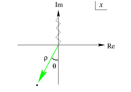
Figure 11: A ray in the complex $x$-plane.

For $M>1$, the leading asymptotic predicted by (4.1) is not changed if $P(x)$ is replaced by $-(ix)^{2M}$, and substituting into the WKB formula we see two possible behaviours, as expected of a second-order ODE:

$$\psi_{\pm}\sim P^{-1/4}\exp\left[\pm{\textstyle\frac{1}{M{+}1}}e^{i\theta(1{+}M)}\rho^{1{+}M}\right]\,.$$ (4.2)

For most values of $\theta$, one of these solutions will be exponentially growing, the other exponentially decaying. But whenever $\Re e[e^{i\theta(1{+}M)}]=0$, the two solutions swap rôles and there is a moment when both oscillate, and neither dominates the other. The relevant values of $\theta$ are

$$\theta=\pm\frac{\pi}{2M{+}2}~{},~{}\pm\frac{3\pi}{2M{+}2}~{},~{}\pm\frac{5\pi}{2M{+}2}~{},~{}\dots~{}.$$ (4.3)

(Confusingly, the rays that these values of $\theta$ define are sometimes called ‘anti-Stokes lines’, and sometimes ‘Stokes lines’. See, for example, [157].)

Whenever one of these lines lies along the positive or negative real axis, the eigenvalue problem as originally stated becomes much more delicate. Increasing $M$ from $1$, the first time that this happens is at $M=2$, the case of the upside-down quartic potential discussed above. But now we see that the problem arose because the line along which the wavefunction was being considered, namely the real axis, happened to coincide with an anti-Stokes line. We also see how the problem can be averted. Since all functions involved are analytic, there is nothing to stop us from examining the wavefunction along some other contour in the complex plane. In particular, before $M$ reaches $2$, the two ends of the contour can be bent downwards from the real axis without changing the spectrum, so long as their asymptotic directions do not cross any anti-Stokes lines in the process. Having thus distorted the original problem, $M$ can be increased through $2$ without any difficulties. The situation for $M$ just bigger than $2$ is illustrated in figure 12, with the anti-Stokes lines shown dashed and the wiggly line a curve along which the wavefunction $\psi(x)$ can be defined.

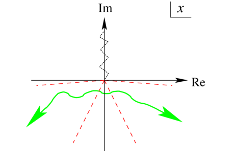
Figure 12: A possible wavefunction contour for $M>2$.

The wedges between the dashed lines are called Stokes sectors, and in directions out to infinity which lie inside these sectors, wavefunctions either grow or decay exponentially, leading to eigenvalue problems with straightforward, and discrete, spectra. Note that once $M$ has passed through $2$, as in figure 12, the real axis is once again a ‘good’ quantisation contour – but for a different eigenvalue problem, which is not the analytic continuation of the original $M<2$ problem to that value of $M$. (For the analogue of figure 2 for this new problem, see figure 20 of [24].) Going further, we could choose any pair of Stokes sectors for the start and finish of our contour. A priori, each pair of sectors defines a different problem, though we shall see later that some of these problems are related by simple variable changes.

All of the problems do share one feature – their quantisation contours begin and end in the neighbourhood of the point $x=\infty$. In the terminology of the WKB method, they are related to ‘lateral’ connection problems [158]. There is one other special point for the ordinary differential equation, namely the origin, and this provides another natural place where quantisation contours can end. Contours which join $x=0$ to $x=\infty$ lead to what are called ‘radial’ (or ‘central’) connection problems, and with suitable boundary conditions they can also have interesting, discrete, spectra. However, if both ends of the contour are placed at $x=0$, the resulting eigenvalue problem is always trivial. Some sample quantisation contours are shown in figure 13.

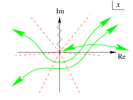
Figure 13: Some further quantisation contours.

We should pause for a moment to consider which boundary conditions can be imposed at the origin, in order to understand why $x=0$ and $|x|=\infty$ behave differently as end points of quantisation contours. Even with the angular-momentum-like term $l(l{+}1)x^{-2}$ included, the singularity at the origin is much milder than that at $|x|=\infty$, and irrespective of the direction in which it is approached, solutions there behave algebraically, as $x^{l+1}$ or $x^{-l}$. For this reason the complications associated with Stokes sectors do not arise in the neighbourhood of the origin, and there are just two natural boundary conditions to impose there – we can either demand that the solution behaves as $x^{l+1}$, or as $x^{-l}$ (the more singular of these two boundary conditions being defined by analytic continuation). This contrasts with the situation near $|x|=\infty$, where we can ask that a solution be subdominant in any one of the potentially infinitely-many different Stokes sectors. Expressed more technically, the ordinary differential equation has two singular points, one at the origin and one at infinity. The singular point at the origin is regular, and solutions have straightforward series expansions in its vicinity. These converge in the full neighbourhood of the origin, and can be analytically continued in a simple way. Infinity, on the other hand, is an irregular singular point, in the neighbourhood of which solutions have asymptotic expansions which only hold in selected Stokes sectors. This makes analytic continuation around the point at infinity much more subtle, and indeed this will be a major theme in the subsequent development.

To summarize: associated with an ODE of the type under consideration there are many natural eigenvalue problems, which fall into two classes. Problems in the first, lateral, class are defined by specifying a pair of Stokes sectors at infinity, and then asking for the values of $E$ at which there exist solutions to the equation which decay exponentially in both sectors simultaneously. Problems in the second, radial, class are defined by demanding decay in a single Stokes sector at infinity, and imposing one of the two simple boundary conditions at the origin. The questions in ${\cal P}{\cal T}$-symmetric quantum mechanics discussed in section 2 are all related to lateral problems, with one particular pair of Stokes sectors selected. Considerations of analytic continuation have led us to put all pairs of sectors on an equal footing, and we completed the story by bringing in the radial problems as well. But at this stage each eigenvalue problem sits on an isolated island, each with its own private spectrum.

In the next subsection, we shall start to construct some bridges between the islands, using methods inspired by earlier work of Sibuya and of Voros. Remarkably, these bridges turn out to be precisely the functional equations which had previously arisen in the context of integrable quantum field theory.

4.2 A simple example

To illustrate the basic ideas in the simplest possible way, for the time being we set $l(l{+}1)=0$, so we are dealing with the original Bender-Boettcher family of eigenproblems:

$$-\frac{d^{2}}{dx^{2}}\psi(x)-(ix)^{2M}\psi(x)=E\psi(x)~{}~{},\qquad\psi\in L^{2}({\cal C})~{}.$$ (4.4)

Now that the perspective has been widened to encompass eigenvalue problems on general contours, it is convenient to eliminate the factors of $i$ appearing everywhere by making the variable changes

$$x\to x/i~{},\quad E\to-E~{}$$ (4.5)

so that the differential equation becomes

$$\left[-\frac{d^{2}}{dx^{2}}+x^{2M}-E\right]\,\psi(x)=0\,.$$ (4.6)

This also moves the branch cut onto the negative real axis, and the initial quantisation contour onto the imaginary axis. (This final point explains why the reality of the spectrum remains a non-trivial question, despite the fact that the coefficients in (4.6) are all real.)

Next, we need to develop our treatment of ordinary differential equations in the complex domain, relying largely on the work of Sibuya and co-workers [161, 20]. The key result is the following:
$\bullet$ The ODE (4.6) has a ‘basic’ solution $y(x,E)$ such that
(i) $y$ is an entire function of $x$ and $E$;

[Though, because of the multivalued potential, $x$ lives on a cover of ${\mathbb{C}}\backslash\{0\}$ if $2M{\notin}{\mathbb{Z}}$ . ]

(ii) as $|x|\to\infty$ with $|\arg\,x\,|<3\pi/(2M{+}2)$,

$$y\, \sim {}~{}\frac{1}{\sqrt{2i}}\,x^{-M/2}\exp\left[-{\textstyle\frac{1}{M{+}1}}\,x^{M{+}1}\right]\,;$$ (4.7)

$$y^{\prime} \sim {-\frac{1}{\sqrt{2i}}}\,x^{M/2}\exp\left[-{\textstyle\frac{1}{M{+}1}}\,x^{M{+}1}\right]\,.$$ (4.8)

[Though there are small modifications for $M\leq 1$ – see, for example, [16] . ]
Furthermore, properties (i) and (ii) fix $y$ uniquely.

The second property can be understood via the WKB discussion of section 4.1. With the shift from $x$ to $x/i$, the anti-Stokes lines for (4.6) are

$$\arg(x)=\pm\frac{\pi}{2M{+}2}~{},~{}\pm\frac{3\pi}{2M{+}2}~{},~{}\dots$$ (4.9)

and in between them lie the Stokes sectors, which we label by defining

$${\cal S}_{k}:=\left|\arg(x)-\frac{2\pi k}{2M{+}2}\right|<\frac{\pi}{2M{+}2}\,.$$ (4.10)

Three of these sectors are shown in the figure 14, a $90^{\rm o}$ rotation of figure 12.

The asymptotic given as property (ii) then matches the result of a WKB calculation in ${\cal S}_{-1}\cup{\cal S}_{0}\cup{\cal S}_{1}$ . The determination of the large $|x|$ behaviour of the particular solution $y(x,E)$ beyond these three sectors is a non-trivial matter, since the continuation of a limit is not necessarily the same as the limit of a continuation. This subtlety is related to the so-called Stokes phenomenon, and it can be handled using objects known as Stokes multipliers, to be introduced shortly.

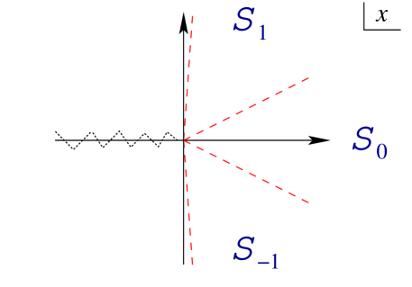
Figure 14: Three Stokes sectors for the ODE (4.6), with $M=2.1$.

One more piece of terminology: an exponentially-growing solution in a given sector is called dominant (in that sector); one which decays there is called subdominant. It is easy to check that $y$ as defined above is subdominant in ${\cal S}_{0}$, and dominant in ${\cal S}_{-1}$ and ${\cal S}_{1}$. A subdominant solution to a second-order ODE in a sector is unique up to a constant multiplier; this is why the quoted asymptotics are enough to pin down $y$ uniquely.

Having identified one solution to the ODE, we can now generate a whole family using a trick due to Sibuya. Consider the function $\hat{y}(x,E):=y(ax,E)$ for some (fixed) $a\in{\mathbb{C}}$. From (4.6), $\hat{y}(x,E)$ satisfies

$$\left[-\frac{d^{2}}{dx^{2}}+a^{2M+2}x^{2M}-a^{2}E\right]\,\hat{y}(x,E)=0\,.$$ (4.11)

(This is sometimes given the rather-grand name of ‘Symanzik rescaling’.) If $a^{2M+2}{=}1$, shifting $E$ to $a^{-2}E$ shows that $\hat{y}(x,a^{-2}E)$ again solves (4.6). Defining

$$\omega:=e^{2\pi i/(2M{+}2)}$$ (4.12)

and

$$y_{k}(x,E):=\omega^{k/2}y(\omega^{-k}x,\omega^{2k}E)$$ (4.13)

we then have the statements

$\bullet$ $y_{k}$ solves (4.6) for all $k\in{\mathbb{Z}}$ ;   [ This follows since $(\omega^{-k})^{2M{+}2}=1$. ]

$\bullet$ up to a constant, $y_{k}$ is the unique solution to (4.6) subdominant in ${\cal S}_{k}$.   [ This follows easily from the asymptotic of $y$. ]

$\bullet$ the functions $y_{k}$, $y_{k+1}$ are linearly independent for all $k$, so each pair $\{y_{k},y_{k+1}\}$ forms a basis of solutions for (4.6).   [ This follows on comparing the asymptotics of $y_{k}$ and $y_{k+1}$ in either ${\cal S}_{k}$ or ${\cal S}_{k+1}$. ]

We have almost arrived at the TQ relation. Next, the fact that $y_{-1}$ can be expanded in the $\{y_{0},y_{1}\}$ basis shows that a relation of the following form must hold:

$$y_{-1}(x,E)=C(E)y_{0}(x,E)+\widetilde{C}(E)y_{1}(x,E)~{}.$$ (4.14)

This is an example of a Stokes relation, with the coefficients $C(E)$ and $\widetilde{C}(E)$ Stokes multipliers. They can be expressed in terms of Wronskians, where [163] the Wronskian of two functions $f$ and $g$ is

$$W[f,g]:=fg^{\prime}-f^{\prime}g\,.$$ (4.15)

Given two solutions $f$ and $g$ of a second-order ODE with vanishing first-derivative term, their Wronskian $W[f,g]$ is independent of $x$, and vanishes if and only if $f$ and $g$ are proportional. As a convenient notation we set

$$W_{k_{1},k_{2}}:=W[y_{k_{1}},y_{k_{2}}]=y_{k_{1}}y_{k_{2}}^{\prime}-y_{k_{1}}^{\prime}y_{k_{2}}$$ (4.16)

and record the following two useful properties:

$$W_{k_{1}+1,k_{2}+1}(E)=W_{k_{1},k_{2}}(\omega^{2}E)~{},\quad W_{0,1}(E)=1\,.$$ (4.17)

Now ‘taking Wronskians’ of the Stokes relation (4.14) first with $y_{1}$ and then with $y_{0}$ shows that

$$C=\frac{W_{-1,1}}{W_{0,1}}~{}~{},\quad\widetilde{C}=-\frac{W_{-1,0}}{W_{0,1}}=-1$$ (4.18)

and so the relation itself can be rewritten as

$$C(E)y_{0}(x,E)=y_{-1}(x,E)+y_{1}(x,E)~{},$$ (4.19)

or, in terms of the original function $y$, as

$$C(E)y(x,E)=\omega^{-1/2}y(\omega x,\omega^{-2}E)+\omega^{1/2}y(\omega^{-1}x,\omega^{2}E)\,.$$ (4.20)

This looks very like a TQ relation. The only fly in the ointment is the $x$-dependence of the function $y$. But this is easily fixed: we just set $x$ to zero. We can also take a derivative with respect to $x$ before setting $x$ to zero, which swaps the phase factors $\omega^{\pm 1/2}$. So we define

$$D_{-}(E):=y(0,E)~{}~{},\quad D_{+}(E):=y^{\prime}(0,E)\,.$$ (4.21)

Then the Stokes relation (4.20) implies

$${}~{}~{}~{}~{}~{}~{}C(E)D_{\mp}(E)=\omega^{\mp 1/2}D_{\mp}(\omega^{-2}\!E)+\omega^{\pm 1/2}D_{\mp}(\omega^{2}\!E)~{},$$ (4.22)

and precisely matches the forms of the TQ equations (3.60) and (3.70) if the twist parameter is set to $\phi=2\pi p=\pi/(2M{+}2)$. Although the details are at this stage sketchy – more will be provided in later sections – we can already see how some concepts in the two worlds of integrable models and ordinary differential equations must be related:

$$\begin{array}[]{|lcl|}\hline\cr&&\\[-9.0pt] {}~{}\parbox{145.10922pt}{Six-vertex model with twist\\ $\phi=2\pi p=\pi/(2M{+}2)$}&&{}\parbox{139.41832pt}{Schr\"{o}dinger equation with\\ homogeneous potential $x^{2M}$}\\[12.0pt] \hline\cr&&\\[-10.0pt] \,\parbox{99.58464pt}{\small Spectral parameter}&{}\!\!\!\!\leftrightarrow}{}{&\mbox{Energy}\\[5.0pt] \,\parbox{99.58464pt}{\small Anisotropy}&{}\!\!\!\!\leftrightarrow}{}{&\mbox{Degree of potential}\\[5.0pt] \,\parbox{99.58464pt}{\small Transfer matrix}&{}\!\!\!\!\leftrightarrow}{}{&\mbox{The Stokes multiplier $C$}\\[6.0pt] \,\parbox{99.58464pt}{\small Q operator}&{}\!\!\!\!\leftrightarrow}{}{&\mbox{$D_{-}(E)$\,: the value of $y(x,E)$ at $x=0$~{}~{}}\\[10.0pt] \hline\cr\end{array}$$

If $y$ on the last line is replaced by $y^{\prime}$, then the twist changes to $\phi=-\pi/(2M{+}2)$.

A small puzzle remains at this stage: why should one particular value of the twist in the integrable model be singled out for a link with an ordinary differential equation? This was resolved shortly after the original observation in [1], when Bazhanov, Lukyanov and Zamolodchikov [2] pointed out that including an angular-momentum-like term $l(l{+}1)/x^{2}$ allowed Q operators at other values of the twist to be matched. The details, and a further small generalisation of the basic ODE (4.6), will be covered in section 5.

4.3 The spectral interpretation

How should we think about $C$ and $D$? In fact they are spectral determinants. The spectral determinant of an eigenvalue problem is a function which vanishes exactly at the eigenvalues of that problem: it generalises to infinite dimensions the characteristic polynomial $\det(M-\lambda{\rm I})$ of a finite-dimensional matrix. Recall that $C(E)$ is equal to the Wronskian $W_{-1,1}(E)$. Thus $C(E)$ vanishes if and only if $W[y_{-1},y_{1}]=0$, in other words if and only if $E$ is such that $y_{-1}$ and $y_{1}$ are linearly dependent. In turn, this is true if and only if the ODE (5.1) has a solution decaying in the two sectors ${\cal S}_{-1}$ and ${\cal S}_{1}$ simultaneously, which is exactly the lateral eigenvalue problem discussed in section 2, modulo the trivial redefinitions of $x$ and $E$. This is enough to deduce that, up to a factor of an entire function with no zeros, $C(E)$ is the spectral determinant for the Bender-Boettcher problem. Even this ambiguity can be eliminated, via Hadamard’s factorisation theorem, once the growth properties of the functions involved have been checked; see [4] for details. By its definition, the zeros of $D_{-}(E)$ are the values of $E$ at which the function $y(x)$, vanishing at $x=\infty$, also vanishes at $x=0$. Likewise, the zeros of $D_{+}(E)$ are the values of $E$ at which $y(x)$ has zero first derivative at $x=0$. Thus $D_{\mp}(E)$ are also spectral determinants. Note that the vanishing of $D_{-}$ or $D_{+}$ corresponds to there existing normalisable wave functions for the equation on the full real axis, with potential $|x|^{2M}$, which are odd or even, respectively, as illustrated in figures 15 and 16; this explains the labelling convention adopted earlier.

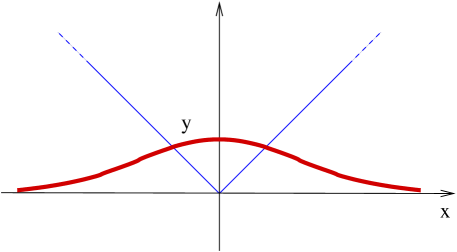
Figure 15: $|x|$-potential, even sector: the ground state wavefunction.

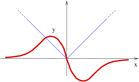
Figure 16: $|x|$-potential, odd sector: the first excited state wavefunction.

This insight allows a gap in the correspondence to be filled. We mentioned in section 3.2 that while the TQ relation is very restrictive, it does not have a unique solution. So to claim that $D_{-}(E)$ is ‘equal’ to $A_{+}(\lambda,p)$ begs the question: which $A_{+}(\lambda,p)$? To answer, we first note that the radial problem for which $D_{-}(E)$ is the spectral determinant, in contrast to the lateral Bender-Boettcher problem, is self-adjoint, and so all of its eigenvalues are guaranteed to be real. Back in the integrable model, we mentioned previously that there is only one solution to the BAE with all roots real, so the question is answered: the relevant $A_{+}(\lambda)$ is that corresponding to the ground state in the spin-zero sector of the model.

5 Completing the dictionary

5.1 Adding angular momentum

We now restore the angular momentum term, and consider the differential equation

$$\Bigl{[}-\frac{d^{2}}{dx^{2}}+x^{2M}+\frac{l(l+1)}{x^{2}}\Bigr{]}\Phi(x)=E\,\Phi(x)\,.$$ (5.1)

This is the ‘$\pi/2$-rotated’ version of the generalised Bender-Boettcher problem (2.5). In the process of discussing this ODE we shall fill in some of the technical details skipped previously. The $l=0$ case was the subject of the first ODE/IM correspondence in [1], while the generalisation to $l\neq 0$ was introduced in [2]. The initial treatment below follows [4].

At the origin, solutions to (5.1) behave as a linear combination of $x^{l+1}$ and $x^{-l}$. As mentioned in section 4.1, a natural eigenproblem for this equation asks for values of $E$ for which there is a solution that vanishes as $x\to+\infty$, and behaves as $x^{l+1}$ as $x\to 0$. In the Stokes/WKB language this is a radial problem. For $\Re e\,l>-1/2$, the condition at the origin is equivalent to the demand that the usually-dominant $x^{-l}$ behaviour there should be absent; outside this region, more care is needed, but the problem can be defined by analytic continuation. This issue will be discussed in more detail in section 5.4 below.

As for the simple example above we first employ Sibuya’s trick. From the uniquely-determined solution $y(x,E,l)$, with large, positive $x$ asymptotic [20]

$$y(x,E,l)\sim\frac{x^{-M/2}}{\sqrt{2i}}\exp\left(-{\textstyle\frac{x^{M+1}}{M+1}}\right),$$ (5.2)

we generate a set of functions

$$y_{k}(x,E,l)=\omega^{k/2}y(\omega^{-k}x,\;\omega^{2k}E,\;l){}~{}~{},\quad\omega=e^{\frac{2\pi i}{2M+2}}{}~{}~{},\quad k\in{\mathbb{Z}}$$ (5.3)

all of which solve (5.1). As before, any pair $\{y_{k},y_{k+1}\}$ forms a basis of the two-dimensional space of solutions, and so $y_{-1}$ can be written as a linear combination of $y_{0}$ and $y_{1}$. Rearranging the expansion and using the properties (4.16), which continue to hold with the addition of the angular-momentum term,

$$C(E,l)\,y_{0}(x,E,l)=y_{-1}(x,E,l)+y_{\;1}(x,E,l)\,,$$ (5.4)

where Stokes multiplier $C(E,l)$ again takes a simple form in the normalisations we have chosen:

$$C(E,l)=W[\,y_{-1}\,,y_{1}]/W[\,y_{0},y_{1}]=W[\,y_{-1}\,,y_{1}]\,.$$ (5.5)

There is one last complication: the angular-momentum term in (5.1) means $x$ cannot simply be set to zero in (5.4) to find a TQ relation. Instead $y$ should be projected onto another solution, defined via its asymptotics as $x\to 0$. Given that solutions near $x=0$ behave as linear combinations of $x^{l{+}1}$ and $x^{-l}$, a solution $\psi(x,E,l)$ can be defined by the requirement

$$\psi(x,E,l)\sim x^{l+1}+O(x^{l+3})\,.$$ (5.6)

This defines $\psi$ uniquely provided $\Re e\,l>-3/2$. A second solution can be obtained from the first by noting that the differential equation – though not the boundary condition – is invariant under the analytic continuation $l\to-1{-}l$. As a result, $\psi(x,E,-1{-}l)$ also solves (5.1). Near the origin, it behaves as $x^{-l}$ , and so at generic values of $l$ the pair of solutions

$$\psi_{+}(x,E) := \psi(x,E,l)\,,$$

$$\psi_{-}(x,E) := \psi(x,E,-1{-}l)$$ (5.7)

are linearly independent. There are some subtleties to this procedure at isolated values of $l$, to which we shall return in section 5.4 below. However, they do not affect the initial argument. In discussions of the radial Schrödinger equation (see, for example, Ch. 4 of [166]), $\psi_{+}$ is sometimes called the regular solution, if $\Re e\,l>-1/2$.

We now take the Wronskian of both sides of (5.4) with $\psi(x,E,l)$ to find an $x$-independent equation:

$$C(E,l)W[y_{0},\psi](E,l)=W[y_{-1},\psi](E,l)+W[y_{1},\psi](E,l)\,.$$ (5.8)

To relate the objects on the right-hand side of this equation back to $W[y_{0},\psi]$, we first define a set of ‘rotated’ solutions by analogy with (5.3):

$$\psi_{k}(x,E,l)=\omega^{k/2}\psi(\omega^{-k}x,\;\omega^{2k}E,\;l)\,,\quad k\in{\mathbb{Z}}\,.$$ (5.9)

These also solve (5.1), and a consideration of their behaviour as $x\to 0$ shows that

$$\psi_{k}(x,E,l)=\omega^{-(l+1/2)k}\psi(x,E,l)\,.$$ (5.10)

In addition,

$$W[y_{k},\psi_{k}](E,l) = \omega^{k}\,W[y(\omega^{-k}x,\omega^{2k}E,l),\psi(\omega^{-k}x,\omega^{2k}E,l)]$$ (5.11)

$$= W[y,\psi](\omega^{2k}E,l)\,.$$

Combining these results,

$$W[y_{k},\psi](E,l)=\omega^{(l{+}1/2)k}W[y,\psi](\omega^{2k}E,l)$$ (5.12)

and so, setting

$$D(E,l):=W[y,\psi](E,l)\,,$$ (5.13)

the projected Stokes relation (5.8) is

$$C(E,l)D(E,l)=\omega^{-(l+1/2)}D(\omega^{-2}E,l)+\omega^{(l+1/2)}D(\omega^{2}E,l)\,.$$ (5.14)

5.2 Matching TQ and CD relations

Finally we are ready to make the precise connection with the TQ relation (3.70). As a shorthand, define

$$D_{\mp}(E):=W[y,\psi_{\pm}](E,l)$$ (5.15)

(so $D_{-}(E)\equiv D(E,l)$ and $D_{+}(E)\equiv D(E,-1{-}l)$). Then (5.14) taken at $l$ and $-1{-}l$ becomes

$$C(E,l)D_{\mp}(E)=\omega^{\mp(2l+1)/2}D_{\mp}(\omega^{-2}E)+\omega^{\pm(2l+1)/2}D_{\mp}(\omega^{2}E)\,.$$ (5.16)

If we set

$$\beta^{2}=\frac{1}{M{+}1}~{}~{},\qquad p=\frac{2l+1}{4M{+}4}$$ (5.17)

then the match between the general TQ relation (3.70) and the Stokes relation (5.16) is perfect, with the following correspondences between objects from the IM and ODE worlds:

$$T~{} \leftrightarrow ~{}C$$

$$Q_{\pm}~{} \leftrightarrow ~{}D_{\mp}~{}.$$

The mapping could also have been made onto the limiting form of the Bethe ansatz equations for the six-vertex model with twisted boundary conditions that was obtained in section 3.5. In this case we have

$$t~{} \leftrightarrow ~{}C$$ (5.18)

$$q~{} \leftrightarrow ~{}D~{},$$

and, as mentioned before, the relationships between the anisotropy parameter $\eta$ and the twist $\phi$ of the lattice model, and the parameters $M$ and $l$ appearing in the potential of the Schrödinger equation are

$$\eta=\frac{\pi}{2}\frac{M}{M{+}1}\quad,\quad\phi=\frac{(2l+1)\pi}{2M+2}~{}.$$ (5.19)

The exact mapping between the functions appearing in these equations can be found by examining the functions at $E=0$ and their asymptotic behaviour at $E=\infty$. Since the behaviour of $D_{+}(E)$ can be deduced from that of $D_{-}(E)\equiv D(E,l)$, we only need the following results [4], which hold for $M>1$:

1. $C$ and $D$ are entire functions of $E$;

2. The zeros of $D$ are all real, and if $l>-1/2$ then they are all positive;

3. The zeros of $C$ are all real, and if $-1-M/2<l<M/2$ then they are all negative;

4. If $M>1$ then the large-$E$ asymptotic of $D$ is

   $$\ln D(E,l)\sim\frac{a_{0}}{2}(-E)^{\,\mu}\quad,\quad|E|\to\infty\quad,\quad|\arg(-E)|<\pi~{},$$ (5.20)

   where $\mu=(M{+}1)/2M$, and $a_{0}=-\,\Gamma{(-\mu)}\Gamma({\mu+\frac{1}{2})}/\sqrt{\pi}~{};$

5. At $E=0$

   $$\ D(E,l)|^{\phantom{p}}_{E=0}=\frac{1}{\sqrt{2i\pi}}\Gamma{(1+{\textstyle\frac{2l+1}{2M+2}})}(2M{+}2)^{\frac{2l+1}{2M+2}+\frac{1}{2}}~{}.$$ (5.21)

6. The large-$E$ asymptotic implies that $D(E,l)$ has order equal to $\mu$, which is strictly less than one for $M>1$. Thus, Hadamard’s factorisation applies in its simplest form and $D(E,l)$ can be represented as:

   $$D(E,l)=D(0,l)\prod_{k=1}^{\infty}\left(1-{E\over E_{k}}\right)$$ (5.22)

Property (i) follows from the definition of $D$ as a Wronskian, since all functions involved are entire functions of $E$. Properties (ii) and (iii) will be proven in section 6.2, while the proof of properties (iv) and (v) can be found in appendix B.

The relevant analytical properties of $T(s)$ and $Q_{+}(s)$ are given in [30, 31]. For $\beta^{2}$ in the semiclassical domain:

1. $T(s,p)$ and $Q_{\pm}(s,p)$ are entire functions of $s$ with an essential singularity at infinity on the real axis;

2. All zeros of $Q_{+}(s,p)$ are real, and if $2p>-\beta^{2}$ they are all strictly positive;

3. All zeros of $T(s,p)$ are real, and if $|p|<1/4$ they are all negative;

4. The large-$s$ asymptotics are

   $$\ \begin{array}[]{lcl}\ln T(s,p)&\!\!\!\!\sim&2\sqrt{\pi}\,\frac{\Gamma{(1-\mu)}}{\Gamma{(\frac{3}{2}-\mu)}}\,\Gamma{\left(\frac{1}{2\mu}\right)}^{2\mu}\,(s)^{\,\mu}\\[10.0pt] \ln Q_{\pm}(s,p)&\!\!\!\!\sim&a_{0}(M{+}1)\,\Gamma{\left(\frac{1}{2\mu}\right)}^{2\mu}\,(-s)^{\,\mu}\end{array}\quad,\quad|s|\to\infty\quad,\quad\arg(-s)<\pi~{},$$ (5.23)

   where $\mu=1/(2{-}2\beta^{2})$ and $a_{0}$ is as defined above;

5. If $s=0$

   $$Q_{+}(0)=1~{}.$$ (5.24)

6. The large-$s$ asymptotic implies that $Q_{\pm}(s)$ has order equal to $1/(2-2\beta^{2})$, which is again strictly less than one for $\beta^{2}$ in the semiclassical domain and we can write

   $$Q_{\pm}(s)=\prod_{k=1}^{\infty}\left(1-{s\over s_{k}}\right)$$ (5.25)

   The restriction of $\beta^{2}$ to the domain $0<\beta^{2}<1/2$ translates to the constraints $\pi/4<\eta<\pi/2$ on the lattice model parameter $\eta$, and we see that the point at which the factorised products have to be regularised coincide in the two cases. For convenience we have only considered $\beta^{2}$ inside the semiclassical domain; see [31, 32, 4] for discussions on the interesting case of $\beta^{2}\geq 1/2$.

Given (5.17), properties (i-iii) and (vi) match the equivalent statements for $T(s,p)$ and $Q_{+}(s,p)$ with $E$ replaced by $s$. Noting that $\mu=(M{+}1)/2M=1/(2{-}2\beta^{2})$, the asymptotic (iv) and the normalisations of $D_{-}$ and $Q_{+}$ can be made to agree by setting

$$\quad\quad\quad s=vE\quad,\quad v=(2M{+}2)^{-1/\mu}\,\Gamma({\textstyle\frac{1}{2\mu}})^{-2}\quad,\quad\gamma_{\mp}=D_{\mp}(0,2p/\beta^{2}{-}{\textstyle\frac{1}{2}})^{-1}~{}.$$ (5.26)

The precise result is [4]

$$Q_{\pm}(s,p)\Bigl{|}_{\beta^{2}} = \gamma_{\mp}\,D_{\mp}({\textstyle\frac{s}{v}},{\textstyle\frac{2p}{\beta^{2}}}{-}{\textstyle\frac{1}{2}})\Bigl{|}_{M=\beta^{-2}{-}1}~{};$$ (5.27)

$$T(s,p)\Bigl{|}_{\beta^{2}} = C({\textstyle\frac{s}{v}},{\textstyle\frac{2p}{\beta^{2}}}{-}{\textstyle\frac{1}{2}})\Bigl{|}_{M=\beta^{-2}{-}1}~{}.$$ (5.28)

5.3 The rôle of the fusion hierarchy

In section 3.7, another set of functional relations found in integrable models was described: the fusion hierarchy. Now that the TQ relation has been mapped onto a Stokes relation, it is natural to ask whether an analogue of the fusion hierarchy can also be found in the differential equation world, and it turns out that this is indeed possible [4].

Previously we examined the expansion of $y_{-1}$ in the basis $\{y_{0},y_{1}\}$, but one can equally ask about the expansion of $y_{k}$ in any other basis, such as $\{y_{k+r-1},y_{k+r}\}$:

$$y_{k-1}=C_{k}^{(r)}y_{k+r-1}+\widetilde{C}_{k}^{(r)}y_{k+r}$$ (5.29)

A change of basis from $\{y_{k+r-1},y_{k+r}\}$ to $\{y_{k-1},y_{k}\}$ can then be encoded in a $2\times 2$ matrix ${\bf C}_{k}^{(r)}$ as

$$\left(\matrix{y_{k-1}\cr y_{k}}\right)={\bf C}^{(r)}_{k}\left(\matrix{y_{k+r-1}\cr y_{k+r}}\right)~{}~{},\quad{\bf C}^{(r)}_{k}=\left(\matrix{C^{(r)}_{k}&\widetilde{C}^{(r)}_{k}\cr C^{(r-1)}_{k+1}&\widetilde{C}^{(r-1)}_{k+1}}\right)\,.$$ (5.30)

This matrix depends on $E$ and $l$, but not $x$. The following properties are immediate:

$${\bf C}^{(r)}_{k}(E,l)={\bf C}^{(r)}_{k-1}(\omega^{2}E,l)~{},$$ (5.31)

$${\bf C}^{(0)}_{k}=\left(\matrix{1&0\cr 0&1}\right)~{}~{},\quad{\bf C}^{(1)}_{k}=\left(\matrix{C_{k}^{(1)}&-1\cr 1&0}\right)~{}.$$ (5.32)

Further relations reflect the fact that the change from the basis $\{y_{k+r+n-1},y_{k+r+n}\}$ to $\{y_{k+r-1},y_{k+r}\}$, followed by the change from $\{y_{k+r-1},y_{k+r}\}$ to $\{y_{k-1},y_{k}\}$, has the same effect as accomplishing the overall change in one go:

$${\bf C}^{(r)}_{k}{\bf C}^{(n)}_{k+r}={\bf C}^{(r+n)}_{k}\,.$$ (5.33)

(These express the consistency of the analytic continuations, and can be thought of as monodromy relations.) The case $r=1$ gives two non-trivial relations:

$$C^{(1)}_{k}C^{(n)}_{k+1}-C^{(n-1)}_{k+2}=C^{(n+1)}_{k}$$ (5.34)

and

$$C^{(1)}_{k}\widetilde{C}^{(n)}_{k+1}-\widetilde{C}^{(n-1)}_{k+2}=\widetilde{C}^{(n+1)}_{k},$$ (5.35)

which can be combined with the ‘initial conditions’ (5.32): to deduce $\widetilde{C}^{(2)}_{k}=-C^{(1)}_{k}\,$; and then the more general equality

$$\widetilde{C}^{(n)}_{k}=-C^{(n-1)}_{k}$$ (5.36)

follows on comparing (5.35) with (5.34). If we now set

$$C^{(n)}(E)=C_{0}^{(n)}(\omega^{-n+1}E)\,,$$ (5.37)

then (5.34) is equivalent to

$$C(E)C^{(n)}(\omega^{n+1\!}E)=C^{(n-1)}(\omega^{n+2\!}E)+C^{(n+1)}(\omega^{n\!}E)\,,$$ (5.38)

and this matches the fusion relation (3.62). Since $C^{(0)}(E)=1=T_{0}(E)$ and, from the last section, $C^{(1)}(E)=C(E)=T_{1/2}(vE)$, this establishes the basic equality

$$C^{(n)}(E)=T_{n/2}(vE)~{}.$$ (5.39)

To find the fusion relation (3.61), we start by taking Wronskians of (5.29) as before to obtain

$$C_{k}^{(r)}=W_{k-1,k+r}\quad,\quad\widetilde{C}_{k}^{(r)}=-W_{k-1,k+r-1}~{},$$ (5.40)

from which we immediately recover (5.36), and can also deduce

$$C_{k}^{(r)}=-C_{k{+}r{+}1}^{(-r-2)}~{}.$$ (5.41)

This relation combined with the $n=-r$ case of (5.33), namely ${\bf C}_{k}^{(r)}{\bf C}_{k+r}^{(-r)}=1$, implies that

$$C^{(r-1)}(\omega^{-1\!}E)C^{(r-1)}(\omega E)-C^{(r)}(E)C^{(r-2)}(E)=1~{},$$ (5.42)

which reproduces the fusion relations (3.61), given the identification (5.39).

Finally, combining (5.39) and (5.40) we have an expression for $T_{n/2}(vE)$ in terms of a Wronskian:

$$T_{n/2}(vE)=C^{(n)}(E)=W_{-1,n}(\omega^{-n+1}E)~{}.$$ (5.43)

This result shows that the fused transfer matrices can also be interpreted as spectral determinants. The right hand side of (5.43) vanishes if and only if $E$ is such that $y_{-1}$ and $y_{n}$ are linearly dependent, which in turn is true if and only if the ODE has a nontrivial solution which simultaneously decays to zero as $|x|\to\infty$ in the sectors ${\cal S}_{-1}$ and ${\cal S}_{n}$. This is one of the lateral eigenvalue problems discussed in section 4.1, with the eigenvalues encoded in the zeros of $C^{(n)}$. The full story is illustrated in figure 17.

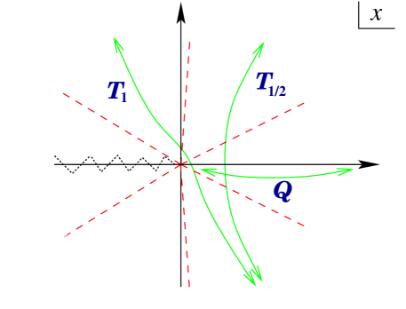
Figure 17: General quantisation contours involved in the ODE/IM correspondence.

Once the fused transfer matrices have been understood in this way, truncation of the fusion hierarchy can be reinterpreted in terms of the (quasi-) periodicity (in $k$) that the functions $y_{k}$ exhibit whenever $M$ is rational [4]. In the simplest cases (with $M$ rational and $l(l{+}1){=}0$) this periodicity arises because the solutions to the ODE live on a finite cover of ${\mathbb{C}}\backslash\{0\}$; for other cases, the monodromy around $x{=}0$ needs a little more care, but the story remains essentially the same.

As a simple example, consider the Schrödinger problems with $2M$ integer and $l(l+1)=0$. In these cases all solutions of the ODE are single-valued functions of $x$, and the sectors ${\cal S}_{n+2M+2}$ and ${\cal S}_{n}$ coincide. Thus both $y_{n}$ and $y_{n+2M+2}$ are subdominant in ${\cal S}_{n}$ and must be proportional. In fact, one can easily show from the asymptotics that $y_{n+2M+2}(x,E,l)=-y_{n}(x,E,l)$, from which we conclude from (5.43) that

$$C^{(2M)}(E)=1\quad,\quad C^{(2M+1)}(E)=0~{}.$$ (5.44)

Thus the set (5.42) of functional relations truncates to

$$C^{(r)}(\omega^{-1}E)C^{(r)}(\omega E)=1+\prod_{n=1}^{2M-1}(C^{(n)}(E))^{G_{nr}}~{},$$ (5.45)

perfectly matching the T-system (3.63).

5.4 The quantum Wronskians

There is one final set of functional relations to discuss: the quantum Wronskian (3.75) and its partner relations (3.74) which express the $T$’s in terms of the $Q$’s. Recall the solutions $\psi_{\pm}$ , defined in equation (5.7) by their behaviour at $x=0$. At generic values of $l$, these give an alternative basis in which to expand $y(x,E,l)$. Using the Wronskian

$$W[\psi_{+},\psi_{-}]=2l+1$$ (5.46)

(evaluated in the limit $x\to 0$), and the relations $D_{\mp}=W[y,\psi_{\pm}]$ ,

$$(2l{+}1)\,y(x,E,l)=D_{-}(E)\,\psi_{-}(x,E)-D_{+}(E)\,\psi_{+}(x,E)\,.$$ (5.47)

Notice that there is a problem with this expansion at $l=-1/2$ , which is easily understood: at this point the two solutions $\psi_{+}$ and $\psi_{-}$ coincide and no longer provide a basis, a fact which is reflected in the vanishing of their Wronskian (5.46). In fact this is not the only place where difficulties arise. So long as $l$ lies in the right half-plane $\Re e\,l>-1/2$, the solution $\psi_{+}(x,E)=\psi(x,E,l)$ can be proved to exist as the limit of a convergent sequence of approximate solutions – see [166, 167, 159]. However, this does not work in the left half-plane, which is another way to see why the second solution $\psi_{-}(x,E)=\psi(x,E,-1{-}l)$ must initially be defined by analytic continuation. At isolated values of $l$ in the left half-plane, poles may arise, causing $\psi_{-}$ to be ill-defined. As discussed in Chapter 4 of [166], these poles can be removed by multiplying $\psi_{-}$ by a regularising factor. However this inevitably inserts extra zeros into the Wronskian (5.46), and the regularised $\widetilde{\psi}_{-}$ fails to be independent of $\psi_{+}$ at exactly the points where the previous $\psi_{-}$ had failed to exist. For the simple power-law potential $x^{2M}$ that we are dealing with, the problem values of $l$ are best identified via the iterative construction of [159], and lead to the conclusion – see for example [4] – that $\{\psi_{+},\psi_{-}\}$ fails to be a basis at the points

$$l+{\textstyle\frac{1}{2}}=\pm(m_{1}+(M{+}1)m_{2})\,,$$ (5.48)

where $m_{1}$ and $m_{2}$ are two non-negative integers. Using (5.17), for the integrable model this corresponds to the twist values

$$2p=\pm(m_{1}\beta^{2}+m_{2})~{}.$$ (5.49)

The set

$$2p=\pm m_{2}~{},~{}~{}(m_{2}=0,1,\dots)$$ (5.50)

corresponds to the vanishing-points for the quantum Wronskian (see eq. (3.75)) and at

$$2p=-\beta^{2}-m_{2}~{},~{}~{}(m_{2}=0,1,\dots)$$ (5.51)

there is a normalisation problem for $Q_{+}(s,p)$ as a consequence of the appearance of a zero level ($s_{k}=0$ for some $k$) [31].

The problem points (5.48) can be dealt with by a limiting procedure – [4] discusses the first case, $l=-1/2$. For now, though, we will assume that $l$ has been picked so that these subtleties do not arise. Then the pair $\{\psi_{+},\psi_{-}\}$ does provide a basis for the ODE, and, using (4.13), we define pairs of solutions $\psi_{k}^{\pm}(x,E)$ as

$$\psi_{k}^{\pm}(x,E)=\omega^{k/2}\psi_{\pm}(\omega^{-k}x,\omega^{2k}E,l)\,,\quad k\in{\mathbb{Z}}\,.$$ (5.52)

These allow the rotated functions $y_{k}$ to be expanded as in (5.47):

$$(2l{+}1)\,y_{k}(x,E,l)=D_{-}(\omega^{2k}E)\,\psi_{k}^{-}(x,E)+D_{+}(\omega^{2k}E)\,\psi_{k}^{+}(x,E)\,.$$ (5.53)

The Wronskians of these solutions are very simple:

$$W[\psi_{k}^{+},\psi_{p}^{+}] = W[\psi_{k}^{-},\psi_{p}^{-}]=0\,,$$ (5.54)

$$W[\psi_{k}^{-},\psi_{p}^{+}] = (2l{+}1)\,\omega^{(k-p)(l+1/2)}\,.$$ (5.55)

The fundamental quantum Wronskian is now almost immediate: in our normalisations, $W[y_{-1},y_{0}]=1$ , and substituting the expansion (5.53) into this formula and using bilinearity of the Wronskian yields

$$(2l+1)=\omega^{-(l+1/2)}D_{-}(\omega^{-1}E)D_{+}(\omega E)-\omega^{l+1/2}D_{-}(\omega E)D_{+}(\omega^{-1}E)~{}.$$ (5.56)

The fused Wronskians are equally straightforward. Taking the Wronskian of $y_{-1}$ and $y_{n}$, again using the expansion (5.53), shifting $E$ to $\omega^{-n+1}E$ and using the relation (5.43) for $C^{(n)}$ shows that

$$(2l+1)C^{(n)}(E) = \omega^{-(n+1)(l+1/2)}D_{-}(\omega^{-n-1}E)D_{+}(\omega^{n+1}E)$$ (5.57)

$$\qquad-\omega^{(n+1)(l+1/2)}D_{-}(\omega^{n+1}E)D_{+}(\omega^{-n-1}E)~{},$$

which is precisely (3.74).

Next we evaluate (5.57) at $l=0$ and $n=M$ for integer $M$, and replace $C^{(M)}$ with $T_{M/2}$ to find

$$\frac{i}{2}\,T_{M/2}(E)=D_{-}(-E,0)D_{+}(-E,0)\equiv D(-E)~{}.$$ (5.58)

The final equality follows from recalling that $D_{-}(E,0)$ and $D_{+}(E,0)$ are the even and odd subdeterminants for the spectral problem defined on the full real axis. This, up to a factor of $i/2$ arising from our normalisation of $D(0)$, is precisely the original result conjectured in [1].

In fact, the quantum Wronksian relation (5.56) was the initial source of the ODE/IM correspondence [1]. As a bridge between the ODE and IM worlds, it has some advantages over the ‘TQ’ approach we have stressed in the foregoing. In particular, it allows for a complete proof of the correspondence [2].

5.5 Numerical techniques

One of the byproducts of the ODE/IM correspondence was the realisation that energy levels for Schrödinger problems can be calculated using nonlinear integral equations [1] of either TBA type or an alternative type known as the Destri de Vega or Klümper-Batchelor-Pearce equations (or simply NLIEs). In appendix D we derive the TBA equations and NLIEs associated with the spectral problems above, and explain how to obtain the spectrum by solving these equations iteratively.

These methods of solving such eigenvalue problems appear to be new, though iterative solution methods based on functional relations for spectral determinants had previously been employed by Voros [21], in work which was an important input to the initial observation of the ODE/IM correspondence in [1]. Numerically, the method is rather efficient – integral equations tend to be easier to solve than differential ones, and spectral determinants encode all the eigenvalues at once.

5.6 The full dictionary

All good correspondences need a dictionary, and the table below summarizes the mapping between objects seen by the integrable model and the differential equation.

$$\begin{array}[]{|lcl|}\hline\cr&&\\[-9.0pt] {}\parbox{85.35826pt}{Integrable\\ Model}&&{}\parbox{93.89418pt}{Schr\"{o}dinger\\ equation}\\[10.0pt] \hline\cr&&\\[-10.0pt] \,\parbox{99.58464pt}{\small Spectral parameter}&{}\!\!\!\!\leftrightarrow}{}{&\parbox{190.63338pt}{\small Energy}\\[5.0pt] \,\parbox{99.58464pt}{\small Anisotropy}&{}\!\!\!\!\leftrightarrow}{}{&\parbox{190.63338pt}{\small Degree of potential}\\[5.0pt] \,\parbox{99.58464pt}{\small Twist parameter}&{}\!\!\!\!\leftrightarrow}{}{&\parbox{190.63338pt}{\small Angular momentum}\\[7.0pt] \,\parbox{99.58464pt}{\small (Fused) transfer\\ matrices}&{}\!\!\!\!\leftrightarrow}{}{&\parbox{190.63338pt}{\small Lateral spectral problems defined at $|x|{=}\infty$}\\[14.0pt] \,\parbox{99.58464pt}{\small $Q$ operators}&{}\!\!\!\!\leftrightarrow}{}{&\parbox{190.63338pt}{\small Radial spectral problems linking $|x|{=}\infty$ and $|x|{=}0$}\\[14.0pt] \,\parbox{99.58464pt}{\small Truncation of the\\ fusion hierarchy}&{}\!\!\!\!\leftrightarrow}{}{&\parbox{190.63338pt}{\small Solutions on finite covers of ${\mathbb{C}}\backslash\{0\}$}\\[10.0pt] \hline\cr\end{array}$$

Armed with the dictionary, the horizontal axis of figure 2 can be annotated to indicate which integrable models correspond to the various values of $M$ in the Bender-Boettcher problem. Thus for $M=\frac{1}{2},1,\frac{3}{2},2$ and $3$, the relevant integrable models are the $N{=}2$ SUSY point of the sine-Gordon model the free-fermion point, the Yang-Lee model, ${\mathbb{Z}}_{4}$ parafermions and the $4$-state Potts model respectively. It is amusing that the $x^{3}$ potential is related by the correspondence to the Yang-Lee model (or, strictly speaking, to the sine-Gordon model at the value of the coupling which allows for a reduction to Yang-Lee), thus returning by a very indirect route to the original thought of Bessis and Zinn-Justin. Note that while the various results discussed here are derived for $M>1$, the ‘Airy case’ ($M=1/2,l=0$) has already been studied in [168], and has been shown to be consistent with integrable field theory predictions [1, 169].

We finish this section with the table below, which records the notation used for the related objects appearing in the six vertex model, the continuum integrable model and the differential equation picture.

$$\begin{array}[]{|lll|}\hline\cr&&\\[-9.0pt] {}\parbox{85.35826pt}{Six vertex\\ model}&{}\parbox{93.89418pt}{Integrable\\ model}&{}\parbox{93.89418pt}{Schr\"{o}dinger\\ equation}\\[10.0pt] \hline\cr&&\\[-10.0pt] {}~{}\nu&s&E\\[5.0pt] {}~{}\eta&\beta&M\\[5.0pt] {}~{}\phi&\phi&l\\[5.0pt] {}~{}t^{(m)}&T_{m}&C^{(2m)}\\[5.0pt] {}~{}q_{0}(\nu,\pm\phi)&Q_{\pm}&D_{\mp}\\[5.0pt] \hline\cr\end{array}$$

6 Applications and generalisations

The correspondence between ordinary differential equations and integrable models is intriguing, but is it good for anything? One answer comes from the fact that the properties of ordinary differential equations and their solutions are rather better understood than those of the $T$ and $Q$ functions from integrable quantum field theory. The correspondence therefore allows a number of conjectured properties of these functions to be proven for the first time – analyticity, duality… [153, 2, 170, 171, 154, 155, 172].

On the other hand, ideas from the theory of integrable models have led to new insights into the spectral properties of a number of quantum-mechanical problems. This section begins with some examples of this aspect, starting with the reality properties in ${\cal P}{\cal T}$-symmetric quantum mechanics that were described back in section 2. First we sketch how the most general class of problems discussed there can be linked with integrable models.

6.1 Inhomogeneous potentials

A key feature of the proof of the TQ relation in section 4 was the fact that the differential equation mapped to itself under the ‘Sibuya’ variable change $x\mapsto\omega^{-1}x$, $E\mapsto\omega^{2}E$, where $\omega{=}\exp(\pi i/(M{+}1))$. In turn, this relied on the ‘potential’ $V(x)=x^{2M}$ being invariant under $V(x)\mapsto\omega^{-2}\,V(\omega^{-1}x)$. A natural generalisation, first observed in [7] and further explored in [11], is to add a term which is exactly anti-invariant under the same transformation. This leads to the consideration of the inhomogeneous potential $V(x)=x^{2M}+\alpha\,x^{M-1}$ and the ordinary differential equation

$$\Bigl{[}-\frac{d^{2}}{dx^{2}}+x^{2M}+\alpha x^{M-1}+\frac{l(l+1)}{x^{2}}\Bigr{]}\Phi(x)=E\,\Phi(x)\,,$$ (6.1)

where $\alpha$ is a free parameter. Again the radial spectral problem asks for those values of $E$ admitting solutions which vanish as $x\to+\infty$, and behave as $x^{l+1}$ as $x\to 0$. With the inclusion of the additional term the subdominant large-$x$ asymptotic, defining the fundamental Sibuya solution, becomes

$$y(x,E,\alpha,l)\sim\frac{x^{-M/2-\alpha/2}}{\sqrt{2i}}\exp\left(-{\textstyle\frac{x^{M+1}}{M+1}}\right).$$ (6.2)

For integer $k$ we then generate a set of solutions to (6.1)

$${}~{}~{}~{}~{}y_{k}(x,E,\alpha,l)=\omega^{k/2+k\alpha/2}y(\omega^{-k}x,\;\omega^{2k}E,\;\omega^{(M+1)k}\alpha,\;l)\quad,\quad\omega=e^{\frac{\pi i}{M+1}}~{},$$ (6.3)

with each pair $\{y_{k},y_{k+1}\}$ forming a basis of solutions. Therefore, just as before, there must be a Stokes relation of the form

$$C(E,\alpha,l)y_{0}(x,E,\alpha,l)=y_{-1}(x,E,\alpha,l)+y_{1}(x,E,\alpha,l)\,,$$ (6.4)

with Stokes multiplier $C(E,\alpha,l)$

$$C(E,\alpha,l)=W[\,y_{-1}\,,y_{1}]/W[\,y_{0},y_{1}]=W[\,y_{-1}\,,y_{1}]~{}.$$ (6.5)

Since $\omega^{M+1}=-1$, the only values of $\alpha$ to arise in the set of functions $y_{k}(x,E,\alpha,l)$, related by (6.4), are $\alpha$ itself, and $-\alpha$. This makes it convenient to define

$$C^{(\pm)}(E):=C(E,\pm\alpha,l)~{},\quad y^{(\pm)}(x,E):=y(x,E,\pm\alpha,l)$$ (6.6)

after which taking (6.4) at positive and negative $\alpha$ implies the pair of coupled equations

$${}~{}~{}C^{(+)}(E)y^{(+)}(x,E)=\omega^{-(1+\alpha)/2}y^{(-)}(\omega x,\omega^{2M}E)+\omega^{(1+\alpha)/2}y^{(-)}(\omega^{-1}x,\omega^{-2M}E)\,,$$ (6.7)

$${}~{}~{}C^{(-)}(E)y^{(-)}(x,E)=\omega^{-(1-\alpha)/2}y^{(+)}(\omega x,\omega^{2M}E)+\omega^{(1-\alpha)/2}y^{(+)}(\omega^{-1}x,\omega^{-2M}E)\,.$$ (6.8)

To remove the $x$-dependence we project onto solutions $\psi_{\pm}(x,E,\alpha,l)$ which are defined at the origin by

$$\psi(x,\alpha,l)=\psi_{+}(x,\alpha,l)\sim x^{l+1}+\dots\quad,\quad x\to 0\,$$ (6.9)

and $\psi_{-}(x,\alpha,l)=\psi(x,\alpha,-1{-}l)$. The subscripts $\pm$ should not be confused with the bracketed superscripts $(\pm)$, which are used to differentiate positive and negative values of $\alpha$. We set

$$D(E,\alpha,l)=W[y,\psi_{+}](E,\alpha,l)~{}.$$ (6.10)

Then, reasoning as before, the Stokes relations (6.7) and (6.8) imply

$${}~{}~{}C^{(+)}(E)D^{(+)}(E)=\omega^{-(2l+1+\alpha)/2}D^{(-)}(\omega^{2M}E)+\omega^{(2l+1+\alpha)/2}D^{(-)}(\omega^{-2M}E)\,,$$ (6.11)

$${}~{}~{}C^{(-)}(E)D^{(-)}(E)=\omega^{-(2l+1-\alpha)/2}D^{(+)}(\omega^{2M}E)+\omega^{(2l+1-\alpha)/2}D^{(+)}(\omega^{-2M}E)\,,$$ (6.12)

where $D^{(\pm)}(E)=D(E,\pm\alpha,l)$ are easily identified with the spectral determinants for the radial problems (6.1) taken at $\pm\alpha$. These equations entwine the spectral problem at $+\alpha$ with that at $-\alpha$, and reduce to two copies of the six-vertex TQ relation for $\alpha=0$. At general $\alpha$ [7] they match equations satisfied by the ${\mathbb{T}}$- and ${\mathbb{Q}}$-operators for the 3-state Perk-Schultz lattice model [173, 174, 175], a model with $U_{q}(\widehat{gl}(2|1))$ symmetry.

6.2 ${\cal P}{\cal T}$-symmetry and reality proofs

For maximal generality, we consider the three-parameter family of Hamiltonians ${\cal H}_{M,\alpha,l}$ and look for solutions of the corresponding Schrödinger equation

$$\left[-\frac{d^{2}}{dx^{2}}-(ix)^{2M}-\alpha(ix)^{M-1}+\frac{l(l+1)}{x^{2}}\right]\psi_{k}(x)=\lambda_{k}\psi_{k}(x)$$ (6.13)

that decay simultaneously at both ends of a contour ${\cal C}$ which can be taken to be the real axis if $M{<}2$, suitably distorted to pass below the origin if $l(l+1)\neq 0$. For larger values of $M$ the contour should be further distorted so as to remain in the pair of Stokes sectors which includes the real axis at $M{=}1$, as illustrated in figure 12 of section 4. We shall prove
Theorem: The spectrum of ${\cal H}_{M,\alpha,l}$ is

• real for $M>1$ and $\alpha<M+1+|2l+1|$ ;

• positive for $M>1$ and $\alpha<M+1-|2l+1|$ .

This result includes the cases considered in section 2.

First we remove the factors of $i$ by setting $\Phi(x)=\psi(x/i)$, so that the Schrödinger problem becomes

$$\ \ \Bigl{[}-\frac{d^{2}}{dx^{2}}+x^{2M}+\alpha x^{M-1}+\frac{l(l+1)}{x^{2}}\Bigr{]}\Phi_{k}(x)=-\lambda_{k}\,\Phi_{k}(x)\,,{}~{}~{}~{}\Phi_{k}(x)\in L^{2}(i{\cal C})\,,$$ (6.14)

and has the same form as (6.1) with $E=-\lambda_{k}$, though with different boundary conditions: to qualify as an eigenfunction, $\Phi$ must decay as $|x|\to\infty$ along the contour $i{\cal C}$. However, it is an easy generalisation of the discussion in section 5 that the function $C(-\lambda,\alpha,l)$ defined in (6.5) is the spectral determinant associated to the spectral problem (6.14). This identification will allow us to prove the theorem using techniques inspired by the Bethe ansatz.

We start from equation (6.11):

$$\qquad C^{(+)}(E)D^{(+)}(E)=\omega^{-(2l+1+\alpha)/2}D^{(-)}(\omega^{-2}E)+\omega^{(2l+1+\alpha)/2}D^{(-)}(\omega^{2}E)\,,$$ (6.15)

and define the zeros of $C^{(+)}(E)=C(E,\alpha,l)$ to be the set $\{-\lambda_{k}\}$, and the zeros of $D^{(\pm)}(E)$ to be the set $\{E^{(\pm)}_{k}\}$. Setting $E=E^{(\pm)}_{k}$ in (6.15) leads back to a (coupled) set of Bethe ansatz equations for the zeros of $D^{(\pm)}$, much as before. However we can also investigate the effect of setting $E=-\lambda_{k}$. The left-hand side of (6.15) is again zero, so the equation can be rearranged to read

$$D^{(-)}(\omega^{2}\lambda_{k})/D^{(-)}(\omega^{-2}\lambda_{k})=-\omega^{-2l-1-\alpha}\,.$$ (6.16)

For $M>1$, WKB estimates show that the function $D^{(-)}(E)$ has order less than one, so that it can be written as a simple product over its zeros, as in (5.22) for the homogeneous potentials. Using this factorised form gives the following set of constraints on the $\lambda_{k}$’s:

$$\prod_{n=1}^{\infty}\left({E^{(-)}_{n}+\omega^{2}\,\lambda_{k}\over E^{(-)}_{n}+\omega^{-2}\,\lambda_{k}}\right)=-\omega^{-2l-1-\alpha}\,,\qquad k=1,2,\dots~{}.$$ (6.17)

Notice what has been achieved here – the little-understood set of numbers $\{\lambda_{k}\}$, eigenvalues of a non-Hermitian eigenvalue problem, are being constrained by the much better-understood set $\{E_{n}^{(-)}\}$ . Since the original eigenproblem (6.13) is invariant under $l\to-1{-}l$, we can assume $l\geq-1/2$ without any loss of generality. Then each $E^{(-)}_{n}$ is an eigenvalue of an Hermitian operator ${\cal H}_{M,-\alpha,l}$, and hence is real. Furthermore a Langer transformation [176] (see also [2, 4]) shows that the $E_{n}^{(-)}$ solve a generalised eigenproblem with an everywhere-positive ‘potential’, and so are all positive, for $\alpha<1{+}2l$. This can be sharpened by considering the value of $D^{(-)}(E)|^{\phantom{p}}_{E=0}$ , found by an easy generalisation of the result obtained in appendix B for the cases with $\alpha=0$. From

$$D^{(\pm)}(E)|^{\phantom{p}}_{E=0}=\sqrt{\frac{2}{i}}\Bigl{(}{\textstyle\frac{M{+}1}{2}}\Bigr{)}^{\frac{2l+1\mp\alpha}{2M+2}+\frac{1}{2}}\frac{\Gamma\left(\frac{2l+1}{M+1}+1\right)}{\Gamma\left(\frac{2l+1\pm\alpha}{2M+2}+\frac{1}{2}\right)}~{}.$$ (6.18)

we see that $D^{(-)}(E)|^{\phantom{p}}_{E=0}$ first vanishes when $\alpha=M{+}2l{+}2$. Until this point is reached, no eigenvalue $E^{(-)}_{n}$ can have passed the origin, and all must be positive. (It might be worried that negative eigenvalues could appear from $E=-\infty$ , but this possibility can be ruled out by a consideration of the Langer-transformed version of the equation.)

Taking the modulus² of (6.17), using the reality of the $E^{(-)}_{k}$, and writing the eigenvalues of (6.13) as $\lambda_{k}=|\lambda_{k}|\exp(i\,\delta_{k})$, we have

$$\prod_{n=1}^{\infty}\left({(E^{(-)}_{n})^{2}+|\lambda_{k}|^{2}+2E^{(-)}_{n}|\lambda_{k}|\cos({\textstyle\frac{2\pi}{M+1}}+\delta_{k})\over(E^{(-)}_{n})^{2}+|\lambda_{k}|^{2}+2E^{(-)}_{n}|\lambda_{k}|\cos({\textstyle\frac{2\pi}{M+1}}-\delta_{k})}\right)=1\,.$$ (6.19)

For $\alpha<M+2l+2$ , all the $E^{(-)}_{n}$ are positive, and each single term in the product on the LHS of (6.19) is either greater than, smaller than, or equal to one depending only on the relative values of the cosine terms in the numerator and denominator. These are independent of the index $n$. Therefore the only possibility to match the RHS is for each term in the product to be individually equal to one, which for $\lambda^{\phantom{p}}_{k}\neq 0$ requires

$$\cos({\textstyle\frac{2\pi}{M+1}}+\delta_{k})=\cos({\textstyle\frac{2\pi}{M+1}}-\delta_{k})\quad\mbox{or}\quad\sin({\textstyle\frac{2\pi}{M{+}1}})\sin(\delta_{k})=0\,.$$ (6.20)

Since $M>1$, this latter condition implies

$$\delta_{k}=m\pi\,,~{}~{}~{}~{}m\in{\mathbb{Z}}$$ (6.21)

and this establishes the reality of the eigenvalues of (6.13) for $M{>}1$ and $\alpha{<}M+2l+2$ or, relaxing the condition on $l$, $\alpha{<}M+1+|2l{+}1|$.

The plots and discussion in section 2 indicate that most of the $\lambda_{k}$ become complex as $M$ falls below $1$, at least for $\alpha=0$. We now see that this coincides with the point at which the order of $D^{(-)}(E)$ is greater than $1$, the factorised form of $D^{(-)}(E)$ provided by Hadamard’s theorem no longer has such a simple form, and the proof just given breaks down.

The borderline case $M=1$ is the simple harmonic oscillator, exactly solvable for all $l$ and $\alpha$ in terms of confluent hypergeometric functions. The case $\alpha=0$ is discussed in detail in appendix B.1; since a nonzero value of $\alpha$ can be absorbed in a simple shift of $E$, it is easily seen that the correctly-normalised solution for the general case is

$$y(x,E,\alpha,l)=\frac{1}{\sqrt{2i}}x^{l+1}e^{-x^{2}/2}U({\textstyle\frac{1}{2}}(l+{\textstyle\frac{3}{2}})-{\textstyle\frac{E-\alpha}{4}},l+{\textstyle\frac{3}{2}},x^{2})\,,$$ (6.22)

and that

$$C(E,\alpha,l)|^{\phantom{p}}_{M=1}=\frac{2\pi}{\Gamma\Bigl{(}\frac{1}{2}+\frac{2l+1+E-\alpha}{4}\Bigr{)}\Gamma\Bigl{(}\frac{1}{2}-\frac{2l+1-E+\alpha}{4}\Bigr{)}}\,.$$ (6.23)

Thus the eigenvalues of (6.13) for $M=1$ are $\lambda_{k}=4k-2-\alpha\pm(2l{+}1)$, $k=1,2,\dots$ . They are all real for all real values of $\alpha$ and $l$, and are all positive for $\alpha{<}2-|2l{+}1|$.

To discuss positivity at general values of $M>1$, we can continue in $M$, $\alpha$ and $l$ away from a point in the region $\{M{=}1,\,\alpha{<}2-|2l{+}1|\}$. So long as $\alpha$ remains less than $M+1+|2l{+}1|$, all eigenvalues will be confined to the real axis during this process, and the first passage of an eigenvalue from positive to negative values will be signalled by the presence of a zero in $C(-\lambda,\alpha,l)$ at $\lambda=0$. Using (6.18) we have

$$C(E,\alpha,l)|^{\phantom{p}}_{E=0}=\Bigl{(}{\textstyle\frac{M{+}1}{2}}\Bigr{)}^{\frac{\alpha}{M+1}}\frac{2\pi}{\Gamma\left(\frac{1}{2}+\frac{2l+1-\alpha}{2M+2}\right)\Gamma\left(\frac{1}{2}-\frac{2l+1+\alpha}{2M+2}\right)}~{},$$ (6.24)

and so the first zero arrives at $E=-\lambda=0$ when $\alpha=M+1-|2l{+}1|$. Thus for all $\alpha{<}M+1-|2l{+}1|$ , the spectrum is entirely positive, as claimed.

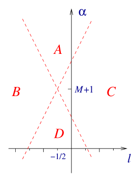
Figure 18: The approximate ‘phase diagram’ at fixed $M$. The proof in the text shows that the spectrum is entirely real in regions $B$, $C$ and $D$, and positive in region $D$.

Referring to the regions $A$, $B$, $C$ and $D$ shown on figure 18, the proof establishes reality for $(\alpha,l)\in B\cup C\cup D$, and positivity for $(\alpha,l)\in D$. This doesn’t mean that the spectrum immediately acquires complex elements when the region $A$ is entered, though. In [12] the shape of the domain of unreality was investigated in more detail, for the special case $M=3$ . (This value was chosen because the ${\cal P}{\cal T}$-symmetric problem is there equivalent to a radial problem, making the numerics a little easier to handle. This equivalence will be explained in the next subsection.)

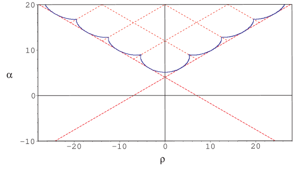
Figure 19: The domain of unreality of ${\cal H}_{3,\alpha,\rho}$, where $\rho=\sqrt{3}(2l{+}1)$. Also shown are segments of the lines along which the problem has a protected zero-energy level.

Figure 19 repeats the plot from [12] already shown in the prelude, this time superimposing the boundaries of regions $A$, $B$, $C$ and $D$. The full domain of unreality (the interior of the cusped line), only touches the borders of region $A$ at isolated points. There is also a small, approximately-triangular region inside $A$ near $\rho=0$ within which the spectrum is entirely real and positive, despite being outside region $D$.

In fact, the condition $\alpha{<}M+1+|2l+1|$, which arose as a technical point in the proof, has a rather more physical explanation [12]. Along the lines $\alpha=M+1\pm(2l+1)$ the problem can be reformulated in terms of a ${\cal P}{\cal T}$-symmetric version of supersymmetric quantum mechanics. On the supersymmetric lines the model has a protected zero-energy state which permits eigenvalues to become degenerate and pair off into complex conjugate pairs. For $M=3$ this occurs at the points where the cusped line touches the borders of $A$ on figure 19.

The idea of a protected zero-energy level also leads to a partial explanation for the pattern of cusps seen in figure 19. In addition to the supersymmetric lines $\alpha=M{+}1\pm(2l{+}1)$, there is a protected zero-energy state along all line segments shown in figure 19: this follows from (6.24), which shows that $C(E,\alpha,l)$ vanishes whenever $\alpha=(M{+}1)(2n+1)\pm(2l{+}1)$, $n=0,1,\dots$ . For $n\geq 1$ these are precisely the lines on which cusps would be expected to be found, as follows from a consideration of the mergings of the relevant levels, and the fact – special to $M=3$ – that the merging levels enjoy an $E\to-E$ symmetry.

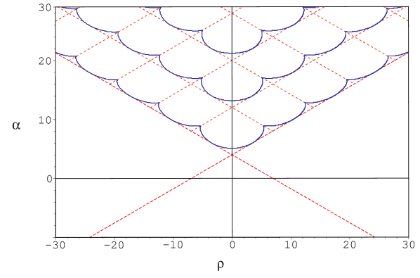
Figure 20: An expanded view of figure 19, showing the frontiers of the regions with zero, two, four and six complex levels.

The cusped line marking the frontier of the zone of reality is in fact only the first of infinitely-many such lines – figure 20 shows some further lines across which pairs of energy levels become complex.

Finally, we remark that Shin has extended the Bethe-ansatz-inspired ideas of the main proof given above to establish spectral reality for a somewhat wider class of non-Hermitian potentials [92, 89].

6.3 Curiosities at $M=3$

The correspondence with Bethe ansatz systems can also reveal unexpected relationships between the spectral properties of apparently very different problems. One set of examples, obtained in [11], connects quantum-mechanical problems via a third-order equation. Consider the radial problem studied in section 6.1 at $M=3$. For later convenience, we also swap $l$ for the variable $\rho:=\sqrt{3}(2l{+}1)$ already used in figure 19, so that the differential equation is

$$\left[-\frac{d^{2}}{dx^{2}}+x^{6}+\alpha x^{2}+\frac{\rho^{2}-3}{12\,x^{2}}\,\right]\Phi(x)=E\,\Phi(x)\,.$$ (6.25)

The spectrum is encoded in the spectral determinant $D(E,\alpha,l)|_{M=3}$.

On the other hand, we can consider a third-order ordinary differential equation:

$$\left[D(g_{2}{-}2)D(g_{1}{-}1)D(g_{0})+x^{3}\,\right]\phi(x)=\frac{3\sqrt{3}}{4}\,E\,\phi(x)$$ (6.26)

where $D(g)\equiv(\frac{d}{dx}-\frac{g}{x})$. Third-order equations of this type are generally associated with $SU(3)$-related Bethe ansatz equations, as shown in [5, 8], but for the particular ‘potential’ $x^{3}$ that appears in (6.26), they collapse onto $SU(2)$-type equations [11]. With the choice

$$g_{0}=1{+}(\alpha{+}\sqrt{3}\rho)/4~{},~{}~{}g_{1}=1{+}\alpha/2~{},~{}~{}g_{2}=1{+}(\alpha{-}\sqrt{3}\rho)/4~{},$$ (6.27)

the collapse is onto the same set of equations as govern the problem (6.25). This leads to a rather remarkable spectral equivalence between pairs of second- and third- order ordinary differential equations. Furthermore, the third-order equation is symmetrical in $\{g_{0},g_{1},g_{2}\}$, a feature which is completely hidden in the original second-order equation. By playing with this symmetry, some novel spectral equivalences can be established between different second-order radial problems, and also between these and certain lateral problems [11]. The parametrisation in terms of $\alpha$ and $\rho$ allows these relations to be expressed in a compact way in terms of certain $2\times 2$ matrices in the Weyl group of $SU(3)$ [100]. With $\boldsymbol{\alpha}=\Big{(}\!\begin{array}[]{c}\alpha\\[-4.0pt] \rho\end{array}\!\Big{)}$ , let

$$\mbox{Radial}(\boldsymbol{\alpha}) = {\rm Spect}\left(\,\mbox{(\ref{eqe2}) with radial boundary conditions}\,\right)$$

$$\mbox{Lateral}(\boldsymbol{\alpha}) = {\rm Spect}\left(\,\mbox{(\ref{eqe2}) with lateral boundary conditions}\,\right)$$

and define matrices ${\mathbb{L}}$ , ${\mathbb{T}}$ and ${\mathbb{L}}{\mathbb{T}}$ by

$$\qquad{\mathbb{L}}=\left(\begin{array}[]{cc}1&0\\ 0&-1\end{array}\right)~{},\quad{\mathbb{T}}=\frac{1}{2}\left(\begin{array}[]{cc}-1&\sqrt{3}\\ \sqrt{3}&\,1\end{array}\right)~{},\quad{\mathbb{L}}{\mathbb{T}}=\frac{1}{2}\left(\!\begin{array}[]{cc}-1&\sqrt{3}\\ -\sqrt{3}&\,-1\end{array}\right).$$ (6.28)

The reflections ${\mathbb{L}}$ and ${\mathbb{T}}$ together generate the Weyl group of $SU(3)$, with their product ${\mathbb{L}}{\mathbb{T}}$ being an anticlockwise rotation in the $(\rho,\alpha)$ plane by $2\pi/3$. The three mappings are illustrated in figure 21. With this notation in place, three simply-stated spectral equivalences hold:

$${\bf(a)}~{}~{}~{}\mbox{Radial}(\boldsymbol{\alpha}) = \mbox{Radial}({\mathbb{T}}\boldsymbol{\alpha})$$

$${\bf(b)}~{}~{}~{}\mbox{Lateral}(\boldsymbol{\alpha}) = \mbox{Lateral}({\mathbb{L}}\boldsymbol{\alpha})$$

$${\bf(c)}~{}~{}~{}\mbox{Lateral}(\boldsymbol{\alpha}) = \mbox{Radial}({\mathbb{L}}{\mathbb{T}}\boldsymbol{\alpha})~{}.$$

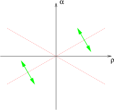
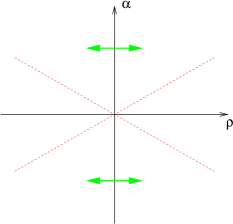
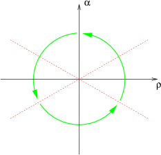
(a) $\boldsymbol{\alpha}\mapsto{\mathbb{T}}\boldsymbol{\alpha}$

(b) $\boldsymbol{\alpha}\mapsto{\mathbb{L}}\boldsymbol{\alpha}$

(c) $\boldsymbol{\alpha}\mapsto{\mathbb{L}}{\mathbb{T}}\boldsymbol{\alpha}$

Figure 21: The three mappings involved in the spectral equivalences.

Of these, the second is trivial – it just encodes the $l\to-1-l$ symmetry of the lateral problem – but the other two are not. The third, (c), gives a direct insight into spectral reality for $M=3$: it demonstrates that the ${\cal P}{\cal T}$-symmetric problem for this case is equivalent to an explicitly Hermitian problem. Notice that the domain of unreality for the ${\cal P}{\cal T}$-symmetric situation – shown in figure 19 above the wavy line – is rotated under (c) into a region of negative $\rho$, where $l$ is sufficiently negative that the radial problem $\mbox{Radial}({\mathbb{L}}{\mathbb{T}}\boldsymbol{\alpha})$ is also non-Hermitian and so no contradiction with unreality arises. (Interestingly, there are similar equivalences [177, 178, 110] for a subset of the non-Hermitian $M=2$ problems, though the methods of proof in those papers are very different.)

In the $(\alpha,\rho)$ coordinates adapted to $M=3$ the lines with a protected zero energy level shown on figure 19 are $\alpha=4J\pm\rho/\sqrt{3}$, $J=1,3,5,\dots$ , and they have an extra significance [12]: they correspond to points at which the model exhibits a ${\cal P}{\cal T}$-symmetric version of the quasi-exact solvability discussed in [179, 180], with an odd number $J$ of ‘QES’ eigenfunctions and eigenvalues which can be found algebraically. In fact, a further spectral equivalence from [11], related to a higher-order supersymmetry [182, 181, 11], can be used to show that if $\boldsymbol{\alpha}$ lies on the line $\alpha=4J+\rho/\sqrt{3}$, with $J$ an integer, then the non-QES part of the ${\cal P}{\cal T}$-symmetric spectrum $\mbox{Lateral}(\boldsymbol{\alpha})$ is the same as the full ${\cal P}{\cal T}$-symmetric spectrum $\mbox{Lateral}({\mathbb{T}}\boldsymbol{\alpha})$. (Likewise, if $\boldsymbol{\alpha}$ lies on $\alpha=4J-\rho/\sqrt{3}$ then there is a mapping of the non-QES spectrum onto $\mbox{Lateral}({\mathbb{L}}{\mathbb{T}}{\mathbb{L}}\boldsymbol{\alpha})$ .) If $\boldsymbol{\alpha}$ is inside the region $A$, so that some levels of $\mbox{Lateral}(\boldsymbol{\alpha})$ might be complex, then, looking at figure 21a, ${\mathbb{T}}\boldsymbol{\alpha}$ must be outside this region. Thus the non-QES part of $\mbox{Lateral}(\boldsymbol{\alpha})$ is real, and so the levels which become complex as $\boldsymbol{\alpha}$ moves into region $A$ through QES values must lie in the solvable part of the spectrum [12]. This complements a similar, but as yet unproven, conjecture concerning quartic QES potentials [183].

6.4 Further generalisations

The ODE/IM correspondence introduced here for $SU(2)$ Bethe-ansatz systems has been extended to a number of other integrable models and ordinary differential equations. To finish, we present a very schematic summary of the integrable models and differential equations involved in correspondences to date. The cited references should be consulted for more details of the models and parameters involved in each case.

• Six-vertex model, $\boldsymbol{su(2)}$ spin-$\boldsymbol{{\textstyle\frac{1}{2}}}$ XXZ quantum chains and the perturbed boundary sine-Gordon model [1, 2, 4, 3]:
  As already described, the ground state of the six-vertex model is related to the spectral properties of the ordinary differential equation

  $$\Bigl{[}-\frac{d^{2}}{dx^{2}}+x^{2M}+\frac{l(l+1)}{x^{2}}-E\Bigr{]}\Psi(x)=0~{}.$$ (6.29)

  This correspondence has been generalised [14] to map the excited states of the integrable model to the following differential equations:

  $$\ \Bigl{[}-\frac{d^{2}}{dx^{2}}+x^{2M}+\frac{l(l+1)}{x^{2}}-2{d^{2}\over dx^{2}}\sum_{k=1}^{L}\ln(x^{2M+2}-z_{k})-E\Bigr{]}\Psi(x)=0~{},$$ (6.30)

  where the constants $\{z_{k}\}$ satisfy

  $$\sum_{{j=1\atop j\neq k}}^{{\atop L}}{z_{k}(z_{k}^{2}+(M{+}3)(2M{+}1)z_{k}z_{j}+M(2M{+}1)z_{j}^{2})\over(z_{k}-z_{j})^{3}}-{Mz_{k}\over 4(M{+}1)}+\Delta=0\,,~{}$$ (6.31)

  and

  $$\Delta={(2l+1)^{2}-4M^{2}\over 16(M{+}1)}~{}.$$ (6.32)

  These equations were also obtained in [184]. Very recently, they and the simpler equation for the ground state have been interpreted as special cases of Langlands duality [185].

• Perk-Schultz models and the perturbed hairpin model of boundary interaction[7, 11, 186]:
  Adding a inhomogeneous term to (6.29) gives the ordinary differential equation discussed in section 6.1:

  $${\Big{[}}-\frac{d^{2}}{dx^{2}}+x^{2M}+\alpha x^{M-1}+\frac{l(l+1)}{x^{2}}-E{\Big{]}}\Psi(x)=0\,.$$ (6.33)

  Via a change of variables this is equivalently

  $$\Bigl{[}-\frac{d^{2}}{dx^{2}}-p^{2}+2q\kappa e^{x}+\kappa^{2}(e^{2x}+e^{-nx})\Bigr{]}\Psi(x)=0\,,$$ (6.34)

  the form that was used in [186].

• Spin-$\boldsymbol{j}$ $\boldsymbol{su(2)}$ quantum chains and the boundary parafermionic sinh-Gordon model[187, 188, 189]:
  The higher spin $su(2)$ chains are found by a process known as fusion, and their ground state Bethe ansatz roots group into characteristic ‘strings’ in the imaginary direction of length $2j$. This behaviour is captured by generalised eigenvalue problems of the form

  $$\Bigl{[}-\frac{d^{2}}{dx^{2}}+(x^{2M}-E)^{2j}+\frac{l(l+1)}{x^{2}}\Bigr{]}\Psi(x)=0$$ (6.35)

  or equivalently

  $$\left[-\frac{d^{2}}{dx^{2}}+\kappa^{2}(e^{-\frac{bx}{Q}}+e^{\frac{x}{bQ}})^{2j}-\xi^{2}\right]\Psi(x)=0$$ (6.36)

  where $Q=b+b^{-1}$. The formation of strings for this equation is discussed in [19].

• $\boldsymbol{su(n)}$ vertex models [5, 6, 8, 170, 187, 19]:
  To encode Bethe ansatz systems related to $su(n)$ with $n>2$, it turns out to be necessary to go to higher-order ordinary differential equations:

  $$\Bigl{[}(-1)^{n}D_{n}({\bf g})-P_{K}(x,E)\Bigr{]}\Psi(x)=0\,,$$ (6.37)

  where ${\bf g}=\{g_{0},g_{1}\,\dots\,g_{n-1}\}$ is a collection of ‘twist’ parameters,

  $$\ D_{n}({\bf g})=D(g_{n-1}-(n{-}1))\,\dots\,D(g_{1}-1)\,D(g_{0})~{},{}~{}~{}~{}D(g)=\left(\frac{d}{dx}-\frac{g}{x}\right)$$ (6.38)

  and

  $$P_{K}(x,E)=(x^{hM/K}-E)^{K}$$ (6.39)

  with $h=n+1$, the dual Coxeter number of $su(n)$, and the integer $K$ gives the degree of fusion of the vertex model.

• Finite spin-$\boldsymbol{j}$ XXZ quantum chains at $\boldsymbol{\Delta=\pm{\textstyle\frac{1}{2}}}$[15]:

  $$\Bigl{[}-\frac{d^{2}}{dx^{2}}-\frac{N(N+1)}{\cosh^{2}x}+\frac{M(M+1)}{\sinh^{2}x}+\sigma^{2}\Bigr{]}\Psi(x)=0\,,$$ (6.40)

  with $\sigma=(m+1)/(2j+2)$.

• Coqblin-Schrieffer model[171]:

  $$\Bigl{[}\left(-i\frac{d}{dx}+h_{1}\right)\dots\left(-i\frac{d}{dx}+h_{n}\right)-e^{n\theta}e^{x}x\Bigr{]}\Psi(x)=0\,.$$ (6.41)

  Notice that, after a variable change, this is a particular case of (6.37).

• Circular Brane[154]:

  $$\Bigl{[}-\frac{d^{2}}{dy^{2}}+h^{2}e^{y}+\kappa^{2}\exp(e^{y})\Bigr{]}\Psi(y)=0\,.~{}$$ (6.42)

• Paperclip models[155, 172]:

  $$\Bigl{[}-\frac{d^{2}}{dx^{2}}-p^{2}{e^{x}\over 1+e^{x}}-(q^{2}-\frac{1}{4}){e^{x}\over(1+e^{x})^{2}}+\kappa^{2}(1+e^{x})^{n}\Bigr{]}\Psi(x)=0\,.~{}$$ (6.43)

  Note, setting $x=y-\log n$ and taking the limit $n\to\infty$ reduces this to (6.42), the circular brane. The paperclip models and the perturbed boundary hairpins of [186] both exhibit the conformal hairpin boundary condition in their ultraviolet limits, but the perturbations are different.

• Finite spin-$\boldsymbol{{\textstyle\frac{1}{2}}}$ XYZ quantum chain (off-critical deformation of the $\boldsymbol{\Delta{=}-{\textstyle\frac{1}{2}}}$ XXZ model)[17]:

  $$6q{\partial\over\partial q}\Psi(x,q)=\Bigl{[}-{\partial^{2}\over\partial x^{2}}+9n(n+1)\raise 1.72218pt\hbox{{\Large$\wp$}}(3x|q^{3})+c(q,n)\Bigr{]}\Psi(x,q)$$ (6.44)

  where $\wp$ is the Weierstrass elliptic function, $q=e^{i\pi\tau}$, $\tau$ is the modular parameter,

  $$c(q,n)=-3n(n+1){\vartheta^{\prime\prime\prime}_{1}(0,q^{3})\over\vartheta^{\prime}_{1}(0,q^{3})}\,,$$ (6.45)

  and $\vartheta_{1}$ is the elliptic theta function.

• $\boldsymbol{so(2n)}$ vertex models[19]:

  $$\ \left[D_{n}({\bf g^{\dagger}})\left(\frac{d}{dx}\right)^{-1}\!D_{n}({\bf g})-\sqrt{P_{K}(x,E)}\left(\frac{d}{dx}\right)\sqrt{P_{K}(x,E)}\,\right]\Psi(x,E,{\bf g})=0\,,$$ (6.46)

  where ${\bf g}=\{g_{0},g_{1}\,\dots\,g_{n-1}\}$ is a set of twist parameters as for $su(n)$,
  ${\bf g}^{\dagger}=\{n{-}1{-}g_{0},n{-}1{-}g_{1},\dots,n{-}1{-}g_{n-1}\}$ , and the generalised potential term $P_{K}(x,E)$ is as in (6.39), but with $h=2n{-}2$.

• $\boldsymbol{so(2n+1)}$ vertex models[19]:

  $$\ \left[D_{n}({\bf g^{\dagger}})D_{n}({\bf g})+\sqrt{P_{K}(x,E)}\left(\frac{d}{dx}\right)\sqrt{P_{K}(x,E)}\,\right]\Psi(x,E,{\bf g})=0\,,$$ (6.47)

  where $P_{K}(x,E)$ is as in (6.39) with $h=2n{-}1$.

• $\boldsymbol{sp(2n)}$ vertex models[19]:

  $$\ \left[D_{n}({\bf g^{\dagger}})\left(\frac{d}{dx}\right)D_{n}({\bf g})-P_{K}(x,E){\left(d\over dx\right)^{-1}}P_{K}(x,E)\,\right]\psi(x,E,{\bf g})=0\,,$$ (6.48)

  where $P_{K}(x,E)$ is as in (6.39) with $h=n{+}1$.

7 Conclusions

The main conclusion of this review can be stated very simply: it is that the ${\bf T}$ and ${\bf Q}$ operators that arise in certain integrable quantum field theories encode spectral data. This gives a novel perspective on the Bethe ansatz, and also a new way to treat spectral problems via the solution of nonlinear integral equations. As an application, we have shown how Bethe ansatz ideas led to a proof of a reality property in ${\cal P}{\cal T}$-symmetric quantum mechanics. Techniques from integrability also shed light on the way that reality is lost [16]. The correspondence has proved useful in the converse direction as well [153, 171, 154, 155].

There are many further problems to be explored, and here we list just a few. First, it will be interesting to find out how many other BA systems can be brought into the correspondence, beyond those listed in section 6.4.

Second, most of the correspondences established to date have concerned massless integrable lattice models, in a field theory limit where the number of sites, and of Bethe ansatz roots, tends to infinity. The first match to a finite lattice system has been reported in [15], linking the Pöschl-Teller (Heun) equation in complex domain and spin-$\frac{L-2}{2}$ XXZ spin chains at special choices of $\Delta$. It would be of interest to extend this result to other models.

Third, while we have concentrated on describing the correspondence for the ground state eigenvalues of the ${\bf T}$ and ${\bf Q}$ operators, a spectral interpretation for the excited state eigenvalues $t_{1}(\nu)$, $t_{2}(\nu)$ and so on has now been found for the massless $SU(2)$-related system in the continuum limit [14]. The complicated distributions of Bethe roots is reflected in the significantly more complicated nature of the Schrödinger problems. In particular the potentials are no longer real, even for the radial problems. Since all eigenvalues satisfy the same functional relations as for the ground state, it is expected that a correspondence for the excited state eigenvalues of all models should exist.

Fourth, it would be of interest to extend the correspondence to encompass massive integrable models, a first step towards this goal having very recently been made in [17].

Finally, we should admit that our observations remain at a rather formal and mathematical level. It is natural to ask whether there is a more physical explanation for the correspondence, but perhaps this question will be easier to answer once some of the other open problems have been resolved.

Acknowledgements –

We would like to thank Carl Bender, Christian Korff, Sergei Lukyanov, Davide Masoero, Rafael Nepomechie, Adam Millican-Slater, Junji Suzuki, André Voros and Miloslav Znojil for useful discussions. This project was partially supported by the European network EUCLID (HPRN-CT-2002-00325), INFN grant TO12, NATO grant number PST.CLG.980424, The Nuffield Foundation grant number NAL/32601, and a grant from the Leverhulme Trust.

Appendix A The algebraic Bethe ansatz

In this appendix, we fill in some details of the Bethe ansatz for the six-vertex model. The technique we describe is called the algebraic Bethe ansatz, an elegant formulation developed by the ‘Leningrad school’, which reveals the rôle of the Yang-Baxter equation in a particularly transparent way. Our presentation borrows heavily from [127], fixing one or two typos; other useful references are [190] and [191]. To keep the discussion self-contained, we begin by recalling some of the definitions from section 3.

The local Boltzmann weights for the model are parametrised in terms of the spectral parameter $\nu$ and the anisotropy $\eta$ as

$$a(\nu,\eta)=\sin(\eta+i\nu)=W\!\!\left[\mbox{$\rightarrow$\raisebox{6.45831pt}{$\uparrow$}\raisebox{-6.45831pt}{$\uparrow$}$\rightarrow$}\right]=W\!\!\left[\mbox{$\leftarrow$\raisebox{6.45831pt}{$\downarrow$}\raisebox{-6.45831pt}{$\downarrow$}$\leftarrow$}\right]~{};$$ (A.1)

$$b(\nu,\eta)=\sin(\eta-i\nu)=W\!\!\left[\mbox{$\rightarrow$\raisebox{6.45831pt}{$\downarrow$}\raisebox{-6.45831pt}{$\downarrow$}$\rightarrow$}\right]=W\!\!\left[\mbox{$\leftarrow$\raisebox{6.45831pt}{$\uparrow$}\raisebox{-6.45831pt}{$\uparrow$}$\leftarrow$}\right]~{};$$ (A.2)

$$c(\nu,\eta)=\sin(2\eta)~{}~{}~{}~{}~{}=W\!\!\left[\mbox{$\rightarrow$\raisebox{6.45831pt}{$\uparrow$}\raisebox{-6.45831pt}{$\downarrow$}$\leftarrow$}\right]=W\!\!\left[\mbox{$\leftarrow$\raisebox{6.45831pt}{$\downarrow$}\raisebox{-6.45831pt}{$\uparrow$}$\rightarrow$}\right]~{},$$ (A.3)

representing the weights $W$ as in figure 22.

Figure 22: The local Boltzmann weights.

From these local weights, a $2^{N}\times 2^{N}$ transfer matrix ${\bf T}^{\boldsymbol{\alpha}^{\prime}}_{\boldsymbol{\alpha}}(\nu)$ is constructed:

$${}~{}~{}{\mathbb{T}}^{\boldsymbol{\alpha}^{\prime}}_{\boldsymbol{\alpha}}(\nu)=\sum_{\{\beta_{i}\}}W\!\!\left[\mbox{$\beta_{1}$\raisebox{6.45831pt}{$\alpha^{\prime}_{1}$}\raisebox{-6.45831pt}{ $\alpha_{1}$}$\beta_{2}$}\right]\!(\nu)\,W\!\!\left[\mbox{$\beta_{2}$\raisebox{6.45831pt}{$\alpha^{\prime}_{2}$}\raisebox{-6.45831pt}{ $\alpha_{2}$}$\beta_{3}$}\right]\!(\nu)\,W\!\!\left[\mbox{$\beta_{3}$\raisebox{6.45831pt}{$\alpha^{\prime}_{3}$}\raisebox{-6.45831pt}{ $\alpha_{3}$}$\beta_{4}$}\right]\!(\nu)\dots W\!\!\left[\mbox{$\beta_{N}$\raisebox{6.45831pt}{$\alpha^{\prime}_{N}$}\raisebox{-6.45831pt}{ $\alpha_{N}$}$\beta_{1}$}\right]\!(\nu)$$ (A.4)

where $\boldsymbol{\alpha}=(\alpha_{1},\alpha_{2}\dots\alpha_{N})$ and $\boldsymbol{\alpha}^{\prime}=(\alpha^{\prime}_{1},\alpha^{\prime}_{2}\dots\alpha^{\prime}_{N})$ are multiindices.

The task of the Bethe ansatz is to find eigenvectors $\Psi$ and eigenvalues $t$ of ${\mathbb{T}}$ , so that

$$\sum_{\boldsymbol{\alpha}^{\prime}}{\mathbb{T}}^{\boldsymbol{\alpha}^{\prime}}_{\boldsymbol{\alpha}}\Psi_{\boldsymbol{\alpha}^{\prime}}=t\,\Psi_{\boldsymbol{\alpha}}~{}.$$ (A.5)

As mentioned in section 3, the first step is to make a well-informed guess as to the form of a putative eigenvector. The algebraic Bethe ansatz makes this guess with the help of an additional piece of machinery, the monodromy matrix ${\cal T}$:

$${}~{}~{}{\cal T}^{\boldsymbol{\alpha}^{\prime}}_{\boldsymbol{\alpha}}(\nu)_{ab}=\sum_{\{\beta_{i}\}}W\!\!\left[\mbox{$a$\raisebox{6.45831pt}{$\alpha^{\prime}_{1}$}\raisebox{-6.45831pt}{ $\alpha_{1}$}$\beta_{2}$}\right]\!(\nu)\,W\!\!\left[\mbox{$\beta_{2}$\raisebox{6.45831pt}{$\alpha^{\prime}_{2}$}\raisebox{-6.45831pt}{ $\alpha_{2}$}$\beta_{3}$}\right]\!(\nu)\,W\!\!\left[\mbox{$\beta_{3}$\raisebox{6.45831pt}{$\alpha^{\prime}_{3}$}\raisebox{-6.45831pt}{ $\alpha_{3}$}$\beta_{4}$}\right]\!(\nu)\dots W\!\!\left[\mbox{$\beta_{N}$\raisebox{6.45831pt}{$\alpha^{\prime}_{N}$}\raisebox{-6.45831pt}{ $\alpha_{N}$}$b$}\right]\!(\nu)$$ (A.6)

The definition of ${\cal T}_{ab}$ differs from that of ${\mathbb{T}}$ in the omission of the sum over one of the horizontal spins, $\beta_{1}$ . Of course, ${\mathbb{T}}$ can immediately be recovered from ${\cal T}_{ab}$ , simply by performing this sum:

$${\mathbb{T}}(\nu)=\sum_{a}{\cal T}(\nu)_{aa}={\cal T}(\nu)_{\rightarrow\,\rightarrow}+{\cal T}(\nu)_{\leftarrow\,\leftarrow}~{}.$$ (A.7)

However, it turns out that important data is also hidden in the off-diagonal elements of ${\cal T}$. As for the transfer matrix, illustrated in figure 8 of section 3, the definition ${\cal T}$ is most easily digested with the aid of a picture, figure 23, where in the second line we used the double lines as a shorthand for the entire collections of lines carrying the multiindices $\boldsymbol{\alpha}$ and $\boldsymbol{\alpha}^{\prime}$.

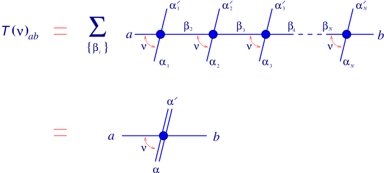
Figure 23: The monodromy matrix.

For convenience, we write the components of ${\cal T}$ as

$${\cal T}(\nu)_{ab}{}~{}{}={}~{}{}\left(\matrix{{\cal T}(\nu)_{\,\rightarrow\,\rightarrow}&{\cal T}(\nu)_{\,\rightarrow\,\leftarrow}\cr{\cal T}(\nu)_{\,\leftarrow\,\rightarrow}&{\cal T}(\nu)_{\,\leftarrow\,\leftarrow}}\right){}~{}{}={}~{}{}\left(\matrix{A(\nu)&B(\nu)\cr C(\nu)&D(\nu)}\right)$$ (A.8)

so that

$${\mathbb{T}}(\nu)=A(\nu)+D(\nu)~{},$$ (A.9)

and, in pictures,

$$A(\nu)={}~{}\raisebox{-17.0pt}{\epsfbox{A.eps}} \qquad B(\nu)={}~{}\raisebox{-17.0pt}{\epsfbox{B.eps}}$$

$$C(\nu)={}~{}\raisebox{-17.0pt}{\epsfbox{C.eps}} \qquad D(\nu)={}~{}\raisebox{-17.0pt}{\epsfbox{D.eps}}$$ (A.10)

As matrices acting on $2^{N}$-dimensional vectors, $A$, $B$, $C$ and $D$ inherit an important property from the microscopic Boltzmann weights by virtue of the ice rule, which preserves the total flux of arrows through each vertex and hence through each collection of vertices. If we define $S$ to be the total number of up arrows minus the total number of down arrows (the ‘spin’), then $A$ and $D$ act on vectors with a definite value of $S$ to give vectors with the same value, while $B$ decreases $S$ by two, and $C$ increases it by two.

We now come to a key property of the Boltzmann weights of the six-vertex model, a sufficient condition for integrability. There exists a collection of numbers $R^{ab}_{cd}(\nu)$, making up the so-called $R$ matrix and related to the Boltzmann weights via $R(\nu)=W(\nu-i\eta)$, such that

$$~{}R^{c^{\prime}\!c}_{aa^{\prime}}(\nu{-}\nu^{\prime})W\!\!\left[\mbox{\small$c\,\,$\raisebox{5.81247pt}{$\delta$}\raisebox{-5.81247pt}{ $\alpha$}$\,\,b$}\right]\!(\nu)\,W\!\!\left[\mbox{\small$c^{\prime}\,\,$\raisebox{5.81247pt}{$\alpha^{\prime}$}\raisebox{-5.81247pt}{ $\delta$}$\,\,\,b^{\prime}$}\right]\!(\nu^{\prime})=W\!\!\left[\mbox{\small$a\,\,$\raisebox{5.81247pt}{$\delta$}\raisebox{-5.81247pt}{ $\alpha$}$\,\,c$}\right]\!(\nu^{\prime})\,W\!\!\left[\mbox{\small$a^{\prime}\,\,$\raisebox{5.81247pt}{$\alpha^{\prime}$}\raisebox{-5.81247pt}{ $\delta$}$\,\,\,c^{\prime}$}\right]\!(\nu)R^{b^{\prime}\!b}_{cc^{\prime}}(\nu{-}\nu^{\prime})~{}.$$ (A.11)

This, a version of the famous Yang-Baxter relation, ‘intertwines’ the local Boltzmann weights at spectral parameters $\nu$ and $\nu^{\prime}$. It is best handled diagrammatically, representing $R^{cd}_{ab}$ as in figure 24.

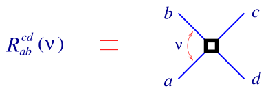
Figure 24: The $R$ matrix.

The perhaps-awkward, but standard, placing of the indices reflects the interpretation of $R$ as a matrix acting on the tensor product $V_{1}\otimes V_{2}$, where $V_{1}$ and $V_{2}$ are the two-dimensional vector spaces, spanned by $\rightarrow$ and $\leftarrow$, that are seen by the indices $c$ and $d$ respectively. The resulting pictorial representation of the intertwining relation is shown in figure 25.

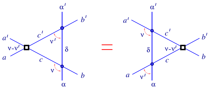
Figure 25: Intertwining the local Boltzmann weights.

Apart from a shift in the spectral parameter, the entries of the $R$ matrix are just the original Boltzmann weights, so in particular they respect the ice rule and the flux of arrows through the ‘$R$’ vertex is conserved. Explicitly, the non-zero entries are

$$R^{\rightarrow\rightarrow}_{\rightarrow\rightarrow}(\nu)=R^{\leftarrow\leftarrow}_{\leftarrow\leftarrow}(\nu) = \raisebox{-17.0pt}{\epsfbox{amat.eps}}=\raisebox{-17.0pt}{\epsfbox{amatr.eps}}=a(\nu{-}i\eta,\eta)=\sin(2\eta{+}i\nu)$$

$$R^{\leftarrow\rightarrow}_{\leftarrow\rightarrow}(\nu)=R^{\rightarrow\leftarrow}_{\rightarrow\leftarrow}(\nu) = \raisebox{-17.0pt}{\epsfbox{bmat.eps}}=\raisebox{-17.0pt}{\epsfbox{bmatr.eps}}=b(\nu{-}i\eta,\eta)=-\sin(i\nu)$$

$$R^{\rightarrow\leftarrow}_{\leftarrow\rightarrow}(\nu)=R^{\leftarrow\rightarrow}_{\rightarrow\leftarrow}(\nu) = \raisebox{-17.0pt}{\epsfbox{cmat.eps}}=\raisebox{-17.0pt}{\epsfbox{cmatr.eps}}=c(\nu{-}i\eta,\eta)=\sin(2\eta)~{}.$$ (A.12)

It is also useful to write $R^{cd}_{ab}(\nu)$ as a $4\times 4$ matrix, with the rows indexed by $ab$ and the columns by $cd$ , and both pairs of indices running $\rightarrow\rightarrow$, $\rightarrow\leftarrow$, $\leftarrow\rightarrow$, $\leftarrow\leftarrow$ :

$$R^{cd}_{ab}(\nu)=\left(\begin{array}[]{cccc}\sin(2\eta{+}i\nu)&0&0&0\\ 0&-\sin(i\nu)&\sin(2\eta)&0\\ 0&\sin(2\eta)&-\sin(i\nu)&0\\ 0&0&0&\sin(2\eta{+}i\nu)\end{array}\right)~{}.$$ (A.13)

This notation makes it easy to check the identity

$$\sum_{e,f}R^{ef}_{ab}(\nu)R^{cd}_{ef}(-\nu)=\sin(2\eta{+}i\nu)\sin(2\eta{-}i\nu)\,\delta^{c}_{a}\delta^{d}_{b}$$ (A.14)

which will be used shortly. (In the parallel universe of integrable quantum field theory, this is related to a property called ‘unitarity’.)

Once the local intertwining relation is known, it is a simple matter to chain together $N$ such equalities to find an analogous relation for the monodromy matrix. This is illustrated in figure 26.

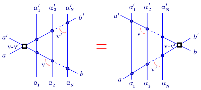
Figure 26: Commuting the monodromy matrices.

In equations, with sums on repeated indices,

$$\qquad~{}~{}R^{c^{\prime}\!c}_{aa^{\prime}}(\nu-\nu^{\prime})({\cal T}^{\boldsymbol{\delta}}_{\boldsymbol{\alpha}})_{cb}(\nu)({\cal T}^{\boldsymbol{\alpha}^{\prime}}_{\boldsymbol{\delta}})_{c^{\prime}b^{\prime}}(\nu^{\prime})=({\cal T}^{\boldsymbol{\delta}}_{\boldsymbol{\alpha}})_{ac}(\nu^{\prime})({\cal T}^{\boldsymbol{\alpha}^{\prime}}_{\boldsymbol{\delta}})_{a^{\prime}c^{\prime}}(\nu)R^{b^{\prime}\!b}_{cc^{\prime}}(\nu-\nu^{\prime})\,.$$ (A.15)

It is usually convenient to leave the fact that each component of ${\cal T}$ is itself a matrix implicit, so that this becomes

$$R^{c^{\prime}\!c}_{aa^{\prime}}(\nu-\nu^{\prime}){\cal T}_{cb}(\nu){\cal T}_{c^{\prime}b^{\prime}}(\nu^{\prime})={\cal T}_{ac}(\nu^{\prime}){\cal T}_{a^{\prime}c^{\prime}}(\nu)R^{b^{\prime}\!b}_{cc^{\prime}}(\nu-\nu^{\prime})\,.$$ (A.16)

Because of the way we have set things up, the ordering of matrices right to left in this equation corresponds to the ordering top to bottom of monodromy matrices in figure 26.

Two important consequences now follow. First, multiplying both sides by $R^{dd^{\prime}}_{b^{\prime}b}(\nu^{\prime}{-}\nu)$, summing on $b$ and $b^{\prime}$, taking traces on $a,d$ and on $a^{\prime},d^{\prime}$, and then finally using the cyclic property of the trace and (A.14) , it can be seen that the transfer matrices at different values of the spectral parameter commute:

$$[{\mathbb{T}}(\nu),{\mathbb{T}}(\nu^{\prime})]=0\,.$$ (A.17)

This establishes the claim made in section 3, and shows that all of the ${\mathbb{T}}(\nu)$ can be diagonalised simultaneously, with $\nu$-independent eigenvectors.

The second consequence is more technical, but crucial for the algebraic Bethe ansatz approach to the construction of eigenvectors. The key idea is to treat $B(\nu)$ as a creation operator, and for this it is necessary to know how to pass the other components of the monodromy matrix through it. Taking the relations implied by figure 26 over all possible values of the vector $(a,a^{\prime},b,b^{\prime})$ of free indices gives a total of $16$ quadratic relations. These can be rearranged to give, amongst others, the following exchange relations:

$$(\rightarrow,\rightarrow,\leftarrow,\leftarrow) : [B(\nu),B(\nu^{\prime})]=0~{};$$ (A.18)

$$(\rightarrow,\leftarrow,\leftarrow,\leftarrow) : D(\nu)B(\nu^{\prime})=g(\nu{-}\nu^{\prime})B(\nu^{\prime})D(\nu)-h(\nu{-}\nu^{\prime})B(\nu)D(\nu^{\prime})~{};$$ (A.19)

and (after swapping $\nu$ and $\nu^{\prime}$)

$$(\rightarrow,\rightarrow,\leftarrow,\rightarrow)~{}~{}:~{}~{}A(\nu)B(\nu^{\prime})=g(\nu^{\prime}{-}\nu)B(\nu^{\prime})A(\nu)-h(\nu^{\prime}{-}\nu)B(\nu)A(\nu^{\prime})~{}.$$ (A.20)

The ‘structure constants’ $g$ and $h$ are related to the components of the $R$ matrix:

$$g(\nu) = \frac{R^{\leftarrow\leftarrow}_{\leftarrow\leftarrow}(\nu)}{R^{\rightarrow\leftarrow}_{\rightarrow\leftarrow}(\nu)}=\frac{a(\nu-i\eta,\eta)}{b(\nu-i\eta,\eta)}=-\frac{\sin(2\eta+i\nu)}{\sin(i\nu)}~{};$$ (A.21)

$$h(\nu) = \frac{R^{\leftarrow\rightarrow}_{\rightarrow\leftarrow}(\nu)}{R^{\rightarrow\leftarrow}_{\rightarrow\leftarrow}(\nu)}=\frac{c(\eta)}{b(\nu-i\eta,\eta)}=-\frac{\sin(2\eta)}{\sin(i\nu)}~{}.$$ (A.22)

One example should illustrate the derivation of these relations. Setting $(a,a^{\prime},b,b^{\prime})=(\rightarrow,\leftarrow,\leftarrow,\leftarrow)$ in figure 26 and recording only the nonvanishing terms in the sums on left and righthand sides,

$$~{}\raisebox{-49.0pt}{\epsfbox{tDa.eps}}~{}+~{}\raisebox{-49.0pt}{\epsfbox{tDb.eps}}~{}=~{}\raisebox{-49.0pt}{\epsfbox{tDc.eps}}$$ (A.23)

Translated into symbols, this is

$$~{}~{}R^{\rightarrow\leftarrow}_{\rightarrow\leftarrow}(\nu-\nu^{\prime})D(\nu)B(\nu^{\prime})+R^{\leftarrow\rightarrow}_{\rightarrow\leftarrow}(\nu-\nu^{\prime})B(\nu)D(\nu^{\prime})=B(\nu^{\prime})D(\nu)R^{\leftarrow\leftarrow}_{\leftarrow\leftarrow}(\nu-\nu^{\prime})$$ (A.24)

which can be quickly rearranged to give (A.19).

At last we can write down some eigenvectors. The first is straightforward: it is the false ferromagnetic ground state $|\Omega\rangle=|\uparrow\,\uparrow\dots\uparrow\,\rangle$. In a vector notation,

$$|\Omega\rangle=\left(\matrix{1\cr 0}\right)\otimes\left(\matrix{1\cr 0}\right)\otimes\left(\matrix{1\cr 0}\right)\dots$$ (A.25)

Since $A$ and $D$ cannot change the value of the spin $S$, and $|\Omega\rangle$ is the unique state with (maximal) spin $N$, it is an eigenvector of both $A$ and $D$. In fact,

$$A(\nu)|\Omega\rangle=a^{N}\!(\nu,\eta)|\Omega\rangle\,,~{}~{}~{}D(\nu)|\Omega\rangle=b^{N}\!(\nu,\eta)|\Omega\rangle\,.$$ (A.26)

On the other hand $C(\nu)|\Omega\rangle=0$ (there is no state with a larger value of $S$) , while $B(\nu)|\Omega\rangle$ is, in general, a new state. For the simplest example, at $N=1$, $|\Omega\rangle=\bigl{(}{1\atop 0}\bigr{)}$ and $A$, $B$, $C$ and $D$ are all $2{\times}2$ matrices:

$$A|^{\phantom{p}}_{N=1}=\left(\matrix{a&0\cr 0&b}\right){}\,,~{}~{}~{}~{}B|^{\phantom{p}}_{N=1}=\left(\matrix{0&0\cr c&0}\right)\,,$$ (A.27)

$$C|^{\phantom{p}}_{N=1}=\left(\matrix{0&c\cr 0&0}\right){}\,,~{}~{}~{}~{}D|^{\phantom{p}}_{N=1}=\left(\matrix{b&0\cr 0&a}\right)\,.$$ (A.28)

Thus $A(\nu)|\Omega\rangle=a(\nu)|\Omega\rangle$, $D(\nu)|\Omega\rangle=b(\nu)|\Omega\rangle$, $C(\nu)|\Omega\rangle=0$, and $B(\nu)|\Omega\rangle=c(\nu)\bigl{(}{0\atop 1}\bigr{)}$. Notice also that $B(\nu)|\Omega\rangle$ would serve as a second eigenvector of ${\mathbb{T}}=A+D$. In fact, in this rather-trivial case it could equally have been $B(\nu^{\prime})|\Omega\rangle$, for (almost) any value of $\nu^{\prime}$. To generalise this observation, at larger values of $N$ one might search for eigenvectors of ${\mathbb{T}}$ of the form

$$|\Psi\rangle=B(\nu_{1})B(\nu_{2})\dots B(\nu_{n})|\Omega\rangle\,.$$ (A.29)

This is the guess mentioned in section 3 as stage (i) of the Bethe ansatz. For $N>1$ this guess (or ansatz) does not always work – extra conditions need to be imposed on the numbers $\nu_{1}\,\dots\nu_{n}$. To find these, we first compute the separate actions of $A(\nu)$ and $D(\nu)$ on our would-be eigenvector $|\Psi\rangle$. Using the $A{-}B$ exchange relation, (A.20),

$$A(\nu)|\Psi\rangle = A(\nu)B(\nu_{1})B(\nu_{2})\dots B(\nu_{n})|\Omega\rangle$$ (A.30)

$$= g(\nu_{1}{-}\nu)B(\nu_{1})A(\nu)B(\nu_{2})\dots B(\nu_{n})|\Omega\rangle$$

$${~{}~{}}-h(\nu_{1}{-}\nu)B(\nu)A(\nu_{1})B(\nu_{2})\dots B(\nu_{n})|\Omega\rangle\,.$$

Continuing to pass $A$ through the $B$ operators, but only recording explicitly those terms resulting from the first term on the right-hand side of (A.20), yields

$$A(\nu)|\Psi\rangle = \prod_{i=1}^{n}g(\nu_{i}-\nu)\,a^{N}\!(\nu,\eta)|\Psi\rangle$$ (A.31)

$${~{}~{}}-h(\nu_{1}{-}\nu)\prod_{i=2}^{n}g(\nu_{i}-\nu_{1})\,a^{N}\!(\nu,\eta)B(\nu)B(\nu_{2})\dots B(\nu_{n})|\Omega\rangle$$

$${~{}~{}}+\mbox{further terms}~{}.$$

A nice way to reconstruct the further terms uses the observation that $|\Psi\rangle$ depends on the parameters $\{\nu_{1}\dots\nu_{n}\}$ in a symmetrical manner, since, from (A.18), the $B(\nu_{j})$ commute. This enables us to deduce that

$$A(\nu)|\Psi\rangle=\Lambda^{+}|\Psi\rangle+\sum_{k=1}^{n}\Lambda^{+}_{k}|\Psi_{k}\rangle$$ (A.32)

where

$$\qquad\Lambda^{+}=a^{N}\!(\nu,\eta)\prod_{j=1}^{n}g(\nu_{j}-\nu)~{},~{}~{}~{}\Lambda^{+}_{k}=-a^{N}\!(\nu_{k},\eta)h(\nu_{k}-\nu)\prod_{j=1\atop j\neq k}^{n}g(\nu_{j}-\nu_{k})$$ (A.33)

and

$$|\Psi_{k}\rangle=B(\nu)\prod_{j=1\atop j\neq k}^{n}B(\nu_{j})|\Omega\rangle~{}.$$ (A.34)

(It is instructive to check this directly, at least for $n=2$.)

The same steps can be repeated to find the action of the matrix $D(\nu)$ on $|\Psi\rangle$, using (A.19) and (A.20). The result is:

$$D(\nu)|\Psi\rangle=\Lambda^{-}|\Psi\rangle+\sum_{k=1}^{n}\Lambda^{-}_{k}|\Psi_{k}\rangle$$ (A.35)

with

$$\qquad\Lambda^{-}=b^{N}\!(\nu,\eta)\prod_{j=1}^{n}g(\nu-\nu_{j})~{},~{}~{}~{}\Lambda^{-}_{k}=-b^{N}\!(\nu_{k},\eta)h(\nu-\nu_{k})\prod_{j=1\atop j\neq k}^{n}g(\nu_{k}-\nu_{j})~{}.$$ (A.36)

The ansatz $|\Psi\rangle$ will be an eigenvector of ${\mathbb{T}}=A+D$ if and only if all terms proportional to $|\Psi_{k}\rangle$ can be made to cancel between $A(\nu)|\Psi\rangle$ and $D(\nu)|\Psi\rangle$ . This requires $\Lambda^{+}_{k}+\Lambda^{-}_{k}=0$ for $k=1\dots n$, or

$$(-1)^{n}\prod_{j=1}^{n}\frac{\sinh(2i\eta-\nu_{k}+\nu_{j})}{\sinh(2i\eta-\nu_{j}+\nu_{k})}=-\frac{a^{N}\!(\nu_{k},\eta)}{b^{N}\!(\nu_{k},\eta)}~{}~{},\qquad k=1\dots n\,.$$ (A.37)

These are the Bethe ansatz equations (BAE) for the roots $\{\nu_{1}\dots\nu_{n}\}$. It is important to reiterate that these equations do not have a unique solution, but rather a discrete set, matching the fact that the matrix ${\mathbb{T}}$ has many eigenvalues. For each self-consistent solution $\{\nu_{i}\}$ of the BAE, the corresponding eigenvector $|\Psi\rangle$ of ${\mathbb{T}}$ has eigenvalue

$$t(\nu) = \Lambda^{+}+\Lambda^{-}$$ (A.38)

$$= a^{N}\!(\nu,\eta)\prod_{j=1}^{n}g(\nu_{j}-\nu)+b^{N}\!(\nu,\eta)\prod_{j=1}^{n}g(\nu-\nu_{j})~{},$$

recovering the formula (3.11) quoted in the main text.

The method can be straightforwardly extended to the more general situation of twisted boundary conditions [28, 128]. The twist described earlier can be implemented by trading

$$W\!\left[\mbox{$\beta_{N}$\raisebox{6.45831pt}{$\alpha^{\prime}_{N}$}\raisebox{-6.45831pt}{ $\alpha_{N}$}$\rightarrow$}\right]\!(\nu){}~{}\longrightarrow~{}~{}e^{-i\phi}~{}W\!\left[\mbox{$\beta_{N}$\raisebox{6.45831pt}{$\alpha^{\prime}_{N}$}\raisebox{-6.45831pt}{ $\alpha_{N}$}$\rightarrow$}\right]\!(\nu)$$ (A.39)

and

$$W\!\left[\mbox{$\beta_{N}$\raisebox{6.45831pt}{$\alpha^{\prime}_{N}$}\raisebox{-6.45831pt}{ $\alpha_{N}$}$\leftarrow$}\right]\!(\nu){}~{}\longrightarrow~{}e^{i\phi}~{}W\!\left[\mbox{$\beta_{N}$\raisebox{6.45831pt}{$\alpha^{\prime}_{N}$}\raisebox{-6.45831pt}{ $\alpha_{N}$}$\leftarrow$}\right]\!(\nu)$$ (A.40)

in the definition (A.6) of the monodromy matrix, so that ${\cal T}(\nu)_{ab}$ becomes

$${\cal T}_{ab}{}~{}{}={}~{}{}\left(\matrix{e^{-i\phi}~{}{\cal T}_{\,\rightarrow\rightarrow}&e^{i\phi}{\cal T}_{\,\rightarrow\leftarrow}\cr e^{-i\phi}~{}{\cal T}_{\,\leftarrow\rightarrow}&e^{i\phi}{\cal T}_{\,\leftarrow\leftarrow}}\right){}~{}{}={}~{}{}\left(\matrix{e^{-i\phi}~{}A(\nu)&e^{i\phi}B(\nu)\cr e^{-i\phi}~{}C(\nu)&e^{i\phi}D(\nu)}\right)~{}.$$ (A.41)

The more general transfer matrix

$${\mathbb{T}}(\nu)=e^{-i\phi}A(\nu)+e^{i\phi}D(\nu)~{},$$ (A.42)

then has eigenvalues

$$t(\nu) = e^{-i\phi}\Lambda^{+}+e^{i\phi}\Lambda^{-}$$ (A.43)

$$= e^{-i\phi}a^{N}\!(\nu,\eta)\prod_{j=1}^{n}g(\nu_{j}-\nu)+e^{i\phi}b^{N}\!(\nu,\eta)\prod_{j=1}^{n}g(\nu-\nu_{j})~{},$$

provided that the set of roots $\{\nu_{1}\dots\nu_{n}\}$ solves the twisted Bethe ansatz equations

$$\qquad(-1)^{n}\prod_{j=1}^{n}\frac{\sinh(2i\eta-\nu_{k}+\nu_{j})}{\sinh(2i\eta-\nu_{j}+\nu_{k})}=-e^{-2i\phi}\frac{a^{N}\!(\nu_{k},\eta)}{b^{N}\!(\nu_{k},\eta)}~{}~{},\qquad k=1\dots n\,.$$ (A.44)

Finally, note that the four-spin reversal invariance of the local Boltzmann weights implies the following property of the transfer matrix:

$${\mathbb{T}}_{\alpha}^{\alpha^{\prime}}(\nu,-\phi)={\mathbb{T}}_{\overline{\alpha}}^{\overline{\alpha}^{\prime}}(\nu,\phi)~{},~{}~{}~{}(\overline{\uparrow}=\downarrow,\overline{\downarrow}=\uparrow)~{}.$$ (A.45)

Indeed, from the definitions (A.1), (A.2), (A.3) and (A.6) we have ${\cal T}^{\boldsymbol{\alpha}^{\prime}}_{\boldsymbol{\alpha}}(\nu)_{\,ab}={\cal T}^{\overline{\boldsymbol{\alpha}}^{\prime}}_{\overline{\boldsymbol{\alpha}}}(\nu)_{\overline{a}\overline{b}}$ and therefore

$$\qquad{\mathbb{T}}^{\boldsymbol{\alpha}^{\prime}}_{\boldsymbol{\alpha}}(\nu,-\phi) = e^{i\phi}~{}{\cal T}^{\boldsymbol{\alpha}^{\prime}}_{\boldsymbol{\alpha}}(\nu)_{\,\rightarrow\rightarrow}+e^{-i\phi}{\cal T}^{\boldsymbol{\alpha}^{\prime}}_{\boldsymbol{\alpha}}(\nu)_{\,\leftarrow\leftarrow}=e^{i\phi}~{}{\cal T}^{\overline{\boldsymbol{\alpha}}^{\prime}}_{\overline{\boldsymbol{\alpha}}}(\nu)_{\,\leftarrow\leftarrow}+e^{-i\phi}{\cal T}^{\overline{\boldsymbol{\alpha}}^{\prime}}_{\overline{\boldsymbol{\alpha}}}(\nu)_{\,\rightarrow\rightarrow}$$ (A.46)

$$= {\mathbb{T}}^{\overline{\boldsymbol{\alpha}}^{\prime}}_{\overline{\boldsymbol{\alpha}}}(\nu,\phi)~{}~{}.$$

A first consequence of the equality (A.45) is that ${\mathbb{T}}(\nu,\phi)$ and ${\mathbb{T}}(\nu,-\phi)$ have the same set of eigenvalues. Furthermore, (A.45) also means that

$${\mathbb{T}}(\nu,-\phi)=U\,{\mathbb{T}}(\nu,\phi)\,U^{-1}~{}~{},~{}~{}U=\overbrace{\sigma_{x}\otimes\sigma_{x}\dots\otimes\sigma_{x}}^{N}$$ (A.47)

where $\sigma_{x}$ is in the vector notation a Pauli matrix. Hence $U^{2}=1$ and the set of eigenvectors of ${\mathbb{T}}(\nu,\phi)$ splits into $U$-invariant singlets and doublets. Invoking the Perron-Frobenius theorem in the spin $0$ sector at $\phi=0$ and continuity we conclude that the ground state is a singlet and its associated eigenvalue $t_{0}(\nu,\phi)$ depends on $\phi$ only through its square:

$$t_{0}(\nu,\phi)=t_{0}(\nu,-\phi)~{}.$$ (A.48)

Appendix B ODE results

This appendix collects some properties of a particular solution of the ordinary differential equation

$$\Bigl{[}-\frac{d^{2}}{dx^{2}}+x^{2M}+\frac{l(l+1)}{x^{2}}\Bigr{]}y(x)=E\,y(x)\,,$$ (B.1)

defined for $M>1$ by the asymptotic

$$y(x)\,\sim{}~{}\frac{1}{\sqrt{2i}}\,x^{-M/2}\exp\left[-{\textstyle\frac{1}{M{+}1}}\,x^{M{+}1}\right]$$ (B.2)

as $x$ tends to infinity in any closed subsector of ${\cal S}_{-1}\cup{\cal S}_{0}\cup{\cal S}_{1}$ , where

$${\cal S}_{k}:=\left|\arg(x)-\frac{2\pi k}{2M{+}2}\right|<\frac{\pi}{2M{+}2}\,.$$ (B.3)

This is the ‘Sibuya solution’, subdominant in ${\cal S}_{0}$ , relevant to the basic ODE/IM correspondence connecting the six-vertex model to an ordinary differential equation.

B.1 The special case of $M=1$

Setting $M=1$ gives the simple harmonic oscillator, exactly solvable for all $l$ in terms of the confluent hypergeometric functions $M(a,b,z)$ and $U(a,b,z)$. The correctly-normalised solution, subdominant in $S_{0}$, is

$$y(x,E,l)=\frac{1}{\sqrt{2i}}\,x^{l+1}e^{-x^{2}/2}U({\textstyle\frac{1}{2}}(l+{\textstyle\frac{3}{2}})-{\textstyle\frac{E}{4}},l+{\textstyle\frac{3}{2}},x^{2})\,,$$ (B.4)

and has the large $x$ asymptotic

$$y(x,E,l)\sim\frac{1}{\sqrt{2i}}\,x^{-1/2+E/2}[1+{\cal O}(x^{-2})]\,e^{-\frac{1}{2}x^{2}}\,.$$ (B.5)

Notice the appearance of an extra factor of $x^{E/2}$ compared with the formula (B.2). This has an interesting effect on the TQ relation [4]. First, the modified asymptotic means that the most natural definition of the shifted solutions $y_{k}(x,E,l)$ is now

$$y_{k}(x,E,l)=\omega^{k/2-kE/2}y(\omega^{-k}x,\;\omega^{2k}E,\;l)~{},\qquad\omega=e^{i\pi/2}~{},$$ (B.6)

since this preserves the property $W_{0,1}(E,l)=1$. The basic Stokes relation (4.19) remains

$$C(E,l)y_{0}(x,E,l)=y_{-1}(x,E,l)+y_{1}(x,E,l)\,,$$ (B.7)

where $C(E,l)=W_{-1,1}(E,l)$. This must be projected onto a solution defined through its behaviour at the origin to eliminate $x$. Define $\psi(x,E,l)$ as in (5.6) through the small-$x$ asymptotic

$$\psi(x,E,l)\sim x^{l+1}+O(x^{l+3})$$ (B.8)

and shifted solutions

$$\psi_{k}(x,E,l)=\omega^{k/2+kE/2}\psi(\omega^{-k}x,\omega^{2k}E,l)\,.$$ (B.9)

The prefactor ensures that $W[y_{k},\psi_{k}](E,l)=W[y,\psi](\omega^{2k}E,l)$ , while a consideration of the small-$x$ behaviour of $\psi_{k}$ shows that $\psi_{k}(x,E,l)=\omega^{-k(l{+}1/2)+kE/2}\psi(x,E,l)$. Hence $W[y_{k},\psi](E,l)=\omega^{k(l{+}1/2)-kE/2}\,W[y,\psi](\omega^{2k}E,l)$. Taking the Wronskian of (B.7) with $\psi$ and setting $D(E,l)=W[y,\psi](E,l)$,

$$\qquad C(E,l)D(E,l)=\omega^{-(l{+}1/2)+E/2}D(\omega^{-2}E,l)+\omega^{(l{+}1/2)-E/2}D(\omega^{2}E,l)\,.$$ (B.10)

The modified asymptotic has resulted in a couple of extra $E$-dependent factors. On the integrable models side of the correspondence, $M=1$ is the free-fermion point and explicit constructions of the $T$ and $Q$ functions had led Bazhanov, Lukyanov and Zamolodchikov to precisely the same ‘renormalisation’ of the TQ relation [31], and so the correspondence survives.

The functions $C$ and $D$ can also be calculated directly from the ordinary differential equation, of course. Taking from [192] the analytic continuation formula

$$\qquad U(a,b,ze^{2\pi in})=(1-e^{-2\pi ibn})\frac{\Gamma(1-b)}{\Gamma(1+a-b)}M(a,b,z)+e^{-2\pi ibn}U(a,b,z)\,,$$ (B.11)

the Wronskian

$$W[U(a,b,z),M(a,b,z)]=\frac{\Gamma(b)}{\Gamma(a)}z^{-b}e^{z}\,,$$ (B.12)

and, for $b>1$, the $|z|\to 0$ asymptotic

$$U(a,b,z)\sim\frac{\Gamma(b-1)}{\Gamma(a)}z^{1-b}+\dots$$ (B.13)

one finds

$$C(E,l)|^{\phantom{p}}_{M=1}=\frac{2\pi}{\Gamma\Bigl{(}\frac{1}{2}+\frac{2l+1+E}{4}\Bigr{)}\Gamma\Bigl{(}\frac{1}{2}-\frac{2l+1-E}{4}\Bigr{)}}$$ (B.14)

and

$$D(E,l)|^{\phantom{p}}_{M=1}=\frac{2\,\Gamma\Bigl{(}l+\frac{3}{2}\Bigr{)}}{\sqrt{2i}\,\Gamma\Bigl{(}\frac{2l+3-E}{4}\Bigr{)}}~{}.$$ (B.15)

The zeros of $D(E,l)$ are at $E=2l-1+4k$, $k=1,2,\dots$ , and reproduce the well-known eigenvalues of the radial simple harmonic oscillator. Zeros of $C(E,l)$ correspond to there being normalisable wavefunctions on a contour which runs along the imaginary axis, save for a diversion to the right of the singularity at $x=0$. A variable-change $x\to x/i$ maps this to the real axis and results in the so-called ${\cal P}{\cal T}$-symmetric simple harmonic oscillator, discussed in [193] and [4]. Since this variable change also negates $E$, the eigenvalues of this problem, from (B.14), are $4k-2\pm(2l{+}1)$, $k=1,2,\dots$ .

B.2 The values of $C(0,l)$ and $D(0,l)$

For general values of $M$, the ordinary differential equation cannot be solved in closed form. However it does simplify at $E=0$, and this allows the value $D(0,l)$ to be found. Observe first that the function

$$\varphi(x)=\left({\textstyle\frac{M{+}1}{2}}\right)^{\frac{M}{2M{+}2}}x^{\frac{M{-}1}{2M{+}2}}\,y\left(\left({\textstyle\frac{M{+}1}{2}}\right)^{\frac{1}{M{+}1}}x^{\frac{2}{M{+}1}},E,l\right)$$ (B.16)

solves the Schrödinger equation

$$\Bigl{[}\,-\frac{d^{2}}{dx^{2}}+x^{2}-\sigma x^{\frac{2-2M}{M+1}}+\frac{\gamma(\gamma+1)}{x^{2}}\,\Bigr{]}\varphi(x)=\Lambda\;\varphi(x)\,,$$ (B.17)

where

$$\sigma=\Bigl{(}{\textstyle\frac{2}{M{+}1}}\Bigr{)}^{\frac{2M}{M+1}}E\,,~{}~{}~{}\gamma=\frac{2l{+}1}{M{+}1}-\frac{1}{2}\,,~{}~{}~{}\Lambda=0~{}.$$ (B.18)

At $E{=}0$, $\sigma$ is zero and (B.17) is the simple harmonic oscillator, which as just described is exactly solvable in terms of the confluent hypergeometric functions $U(a,b,z)$ and $M(a,b,z)$. The correctly-normalised solution, subdominant in the sector ${\cal S}_{0}$, is

$$\varphi(x)|^{\phantom{p}}_{E=0}=\frac{1}{\sqrt{2i}}\,x^{\gamma+1}\,e^{-x^{2}/2}\,U\left(\,{\textstyle\frac{1}{2}}(\gamma{+}{\textstyle\frac{3}{2}}),\gamma{+}{\textstyle\frac{3}{2}},x^{2}\,\right).$$ (B.19)

Reversing the variable changes, extracting the leading behaviour as $x\to 0$ and comparing with (5.13), we find

$$\ D(E,l)|^{\phantom{p}}_{E=0}=\frac{1}{\sqrt{2i\pi}}\Gamma{(1+{\textstyle\frac{2l+1}{2M+2}})}(2M{+}2)^{\frac{2l+1}{2M+2}+\frac{1}{2}}\,.$$ (B.20)

The value of $C(0,l)$ is easier to find: from (5.14) at $E=0$,

$$C(E,l)|^{\phantom{p}}_{E=0}=2\cos\left(\frac{2l{+}1}{2M{+}2}\pi\right).$$ (B.21)

B.3 The large-$E$ behaviour of $D(E,l)$

Given that $\psi(x,E,l)$ is defined to have small-$x$ behaviour $\psi(x,E,l)\sim x^{l+1}$, the Wronskian $D(E,l)\equiv W[y(x,E,l),\psi(x,E,l)]$ can be evaluated for $\Re e\,l>-1/2$ as

$$D(E,l)=\lim_{x\rightarrow 0}\left[(2l{+}1)x^{l}\,y(x,E,l)\right],$$ (B.22)

where

$$\left[-\frac{d^{2}}{dx^{2}}+x^{2M}+\frac{l(l+1)}{x^{2}}-E\right]y=0\,.$$ (B.23)

For this subsection the aim is to find the leading behaviour of $D(E,l)$ as $|E|\to\infty$. As observed by Langer [176], the usual WKB approximation cannot be applied directly in this situation because of the singularity at $x=0$. Instead, Langer suggested making the variable change $x=e^{z}$ , $y(x)=e^{z/2}\phi(z)$ . Setting $\lambda=l+1/2$ the equation becomes

$$\left[-\frac{d^{2}}{dz^{2}}+R(z,E,\lambda)\right]\phi=0$$ (B.24)

where $R(z,E,\lambda)=e^{2z/g}-Ee^{2z}+\lambda^{2}$ and we set $g=1/(M{+}1)$. The general WKB approximation for $\phi$ is

$$\ \frac{A}{R(z,E,\lambda)^{1/4}}\exp\!\left[\int_{z_{0}}^{z}\!\!\sqrt{R(u,E,\lambda)}\,du\right]+\frac{B}{R(z,E,\lambda)^{1/4}}\exp\!\left[-\!\!\int_{z_{0}}^{z}\!\!\sqrt{R(u,E,\lambda)}\,du\right]~{}$$ (B.25)

where $z_{0}$ is an arbitrary constant. Provided $\arg(-E)<\pi$, this WKB expression is valid for all real $z$ (and thus for $x$ all the way down to zero) since $R^{-3/4}(R^{-1/4})^{{}^{\prime\prime}}$ tends to zero uniformly in $z$ as $|E|\to+\infty$ (see [158] for more discussion of the validity of the WKB approximation). The solution we aim to approximate is subdominant as $x\to+\infty$, which requires $A=0$. The value of $B$ is fixed by the large-$x$ asymptotic (B.2). It is convenient to set $z_{0}=+\infty$, in which case the correctly-normalised approximate solution can be written for $M>1$ ($g<1/2$) as [4]

$$\phi^{\rm{WKB}}(z,E,\lambda)=$$ (B.26)

$$\qquad\frac{1}{\sqrt{2i}\,R(z,E,\lambda)^{1/4}}\exp\!\left(\int_{z}^{\infty}\!\!\left[\sqrt{R(u,E,\lambda)}-e^{u/g}\,\right]du-g\,e^{z/g}\right).$$

Substituting into (B.22) gives the WKB approximation to the spectral determinant:

$$\quad D^{\rm{WKB}}(E,l) = \lim_{z\rightarrow-\infty}\left[2\lambda\,e^{\lambda z}\,\phi^{\rm{WKB}}(z,E,l)\right]$$

$$= \sqrt{\frac{2\lambda}{i}}\,\lim_{z\rightarrow-\infty}\left[\exp\left(\lambda z+\int_{z}^{\infty}\!\left[\sqrt{R(u,E,\lambda)}-e^{u/g}\,\right]du\right)\right].$$ (B.27)

To eliminate extraneous factors it is convenient to divide through by $D^{\rm WKB}(0,l)$, giving

$$\frac{D^{\rm WKB}(E,l)}{D^{\rm WKB}(0,l)}=\exp(I(E,\lambda))$$ (B.28)

where

$$I(E,\lambda)=\int_{-\infty}^{\infty}\left[\sqrt{e^{2u/g}-Ee^{2u}+\lambda^{2}}-\sqrt{e^{2u/g}+\lambda^{2}}\,\right]du\,.$$ (B.29)

The remaining step is to analyse this expression as $|E|\to\infty$ with $\arg(-E)<\pi$. Changing variables $u\to u+\frac{g}{2-2g}\ln(-E)$ and setting $\mu=1/(2{-}2g)=(M{+}1)/(2M)$ ,

$$I(E,\lambda) = (-E)^{\mu}\!\int_{-\infty}^{\infty}\left[\sqrt{e^{2u/g}+e^{2u}+\lambda^{2}(-E)^{-2\mu}}-\sqrt{e^{2u/g}+\lambda^{2}(-E)^{-2\mu}}\,\right]du$$ (B.30)

$$\sim (-E)^{\mu}\!\int_{-\infty}^{\infty}\left[\sqrt{e^{2u/g}{+}e^{2u}}-e^{u/g}\,\right]du=(-E)^{\mu}\!\int_{0}^{\infty}\left[\sqrt{t^{2M}{+}1}-t^{M}\right]dt\,.$$

Performing the integral then gives the result quoted in the main text:

$$\ln D(E,l)\sim\frac{a_{0}}{2}(-E)^{\mu}\quad,\quad|E|\to\infty\quad,\quad|\arg(-E)|<\pi~{},$$ (B.31)

where

$$a_{0} = \frac{1}{\sqrt{\pi}}\,\Gamma{(-{\textstyle\frac{1}{2}}{-}{\textstyle\frac{1}{2M}})}\,\Gamma{(1{+}{\textstyle\frac{1}{2M}})}$$ (B.32)

$$= \frac{-1}{\sqrt{\pi}}\,\Gamma{(-\mu)}\,\Gamma{(\mu+{\textstyle\frac{1}{2}})}\quad,\quad\mu=(M{+}1)/2M~{}.$$

Notice that this result is independent of $l$, and applies equally to $D_{-}(E,l)\equiv D(E,l)$ and (after analytic continuation) to $D_{+}(E,l)\equiv D(E,-1{-}l)$.

B.4 The ‘small-$E$/large-$l$’ asymptotic of $\ln D(E,l)$.

The Langer-transformed equation can also be used to extract the large-$l$ behaviour of the spectral determinant, a piece of data which is relevant for matching solutions of the quantum Wronskian equation. Once the initial differential equation for $y(x,E,l)$ has been transformed into the equivalent Schrödinger problem (B.24), the rôle of the energy parameter is taken by $-\lambda^{2}$, and the WKB approximation is thus good in the large-$l$ limit, in addition to the large-$E$ limit investigated above. It is therefore possible to study the large-$l$ behaviour of $D(E,l)$ with standard semiclassical techniques. We start with the WKB expression (B.28) for the ratio $D^{\rm{WKB}}(E,l)/D^{\rm{WKB}}(0,l)$, and expand the integrand of $I(E,\lambda)$ about $E=0$ as

$$\quad\sqrt{e^{2u/g}-Ee^{2u}+\lambda^{2}}-\sqrt{e^{2u/g}+\lambda^{2}}=-\sum_{n=1}^{\infty}{(2n-3)!!\over n!2^{n}}{E^{n}e^{2nu}\over\left(e^{2u/g}+\lambda^{2}\right)^{n-1/2}}~{},$$ (B.33)

so that

$$I(E,\lambda)=-\sum_{n=1}^{\infty}b_{n}(\lambda)E^{n}~{},$$ (B.34)

where the coefficients $b_{n}$ can be written in terms of standard Beta integrals:

$$b_{n}(\lambda) = {(2n-3)!!\over n!\,2^{n}}\int_{-\infty}^{\infty}{e^{2n\theta}\over\left(e^{2\theta/g}+\lambda^{2}\right)^{n-1/2}}\,d\theta$$ (B.35)

$$= \lambda^{1-2n+2ng}\left({g\over 4\,n!\sqrt{\pi}}\right)\Gamma(ng)\Gamma(-1/2+n(1-g))~{}.$$

To ease comparison with C, we also give this result in integrable models notation, using the dictionary entries

$$\lambda=2p/g~{}~{},~{}~{}E=\Gamma^{2}(1{-}g)\left({2\over g}\right)^{\!2-2g}s$$ (B.36)

to find

$$\ln\frac{D^{\rm{WKB}}(E,l)}{D^{\rm{WKB}}(0,l)}=-\sum_{n=1}^{\infty}a_{n}(p)\,s^{n}$$ (B.37)

where in the limit $p\gg 1$

$$a_{n}(p)\sim b_{n}(2p/g)\,\Gamma^{2n}(1{-}g)\left({2\over g}\right)^{\!2n-2ng}=\alpha_{n}\,p^{1-2n+2ng}~{},$$ (B.38)

$$\alpha_{n}={\Gamma(ng)\Gamma(-1/2+n(1{-}g))\over 2n!\sqrt{\pi}}\Gamma^{2n}(1{-}g)~{},$$ (B.39)

matching the results quoted in [153] and in (C.2).

Appendix C Quantum Wronskians and the Weiner-Hopf method

In this appendix we show how the quantum Wronskian allows the power series expansions of the functions $\ln Q_{\pm}$ to be pinned down uniquely, following Appendix A of [153]. A useful background reference for the Weiner-Hopf method is [194]. The proof relies on the following properties of $Q(s,p)$:

1. The function $\ln Q_{+}(s,p)$ has a formal power series expansion

   $$\ln Q_{+}(s,p)=-\sum_{n=1}^{\infty}a_{n}(p)\,s^{n}~{}.$$ (C.1)

2. The coefficients $a_{n}(p)$ are meromorphic functions of $p$, analytic in the half-plane $\Re e(2p)>-g$, where $g=\beta^{2}$ so $q=e^{i\pi g}$.

3. As $p\to\infty$ in the right half-plane,

   $$a_{n}(p)\sim\alpha_{n}\,p^{1-2n+2ng}$$ (C.2)

   with

   $$\alpha_{1}=\frac{1}{2\sqrt{\pi}}\Gamma(g)\Gamma(\frac{1}{2}-g)\Gamma(1-g)^{2}.$$ (C.3)

4. $Q_{-}$ is related to $Q_{+}$ as

   $$Q_{-}(s,p)=Q_{+}(s,-p)=\exp\left(-\sum_{n=1}^{\infty}a_{n}(-p)\,s^{n}\right).$$ (C.4)

5. The quantum Wronskian condition holds:

   $$e^{2\pi ip}Q_{+}(qs,p)\,Q_{-}(q^{-1}s,p)-e^{-2\pi ip}Q_{+}(q^{-1}s,p)\,Q_{-}(qs,p)=2i\sin(2\pi p)~{}.$$ (C.5)

These properties lead to a sequence of problems of Weiner-Hopf type which fix the coefficients $a_{n}(p)$ uniquely, as follows.

First, substituting the power series (C.1) and (C.4) into the quantum Wronskian (C.5) gives

$$\qquad e^{2\pi ip}\exp\left(-\sum_{n=1}^{\infty}(q^{n}a_{n}(p)+q^{-n}a_{n}(-p))s^{n}\right)$$

$$\qquad\qquad\qquad{}-e^{-2\pi ip}\exp\left(-\sum_{n=1}^{\infty}(q^{-n}a_{n}(p)+q^{n}a_{n}(-p))s^{n}\right)=2i\sin(2\pi p)~{}.\qquad$$ (C.6)

Expanding and equating coefficients leads to a set of relations of the form

$$\sin(\pi ng+2\pi p)a_{n}(p)-\sin(\pi ng-2\pi p)a_{n}(-p)=R_{n}(p)\,,\quad n=1,2,\dots~{}$$ (C.7)

where each function $R_{n}(p)$ can be expressed in terms of $a_{k}(\pm p)$ with $k=1\dots n{-}1$. For example,

$$R_{1} = 0$$ (C.8)

$$R_{2} = -(q\;a_{1}(p)+q^{-1}a_{1}(-p))^{2}e^{4\pi ip}\sin(2\pi p)/2~{}.$$ (C.9)

Let’s consider a homogeneous case first, setting $R_{n}=0$. Then (C.7) can be rewritten as

$$\frac{\Gamma(1-ng+2p)}{\Gamma(ng+2p)}\,a_{n}(p)=\frac{\Gamma(1-ng-2p)}{\Gamma(ng-2p)}\,a_{n}(-p)$$ (C.10)

The left-hand side of this equation is analytic in the right half-plane $\Re e(2p)>-g$, and the right-hand side is analytic in the left half-plane $\Re e(2p)<g$. The common strip of analyticity $-g<\Re e(2p)<g$ ensures that both sides correspond to a single function $f_{n}(p)$ which is therefore entire: it is analytic on the whole complex plane. Furthermore, combining $\Gamma(z+a)/\Gamma(z+b)\sim z^{a-b}$ with the asymptotic (C.2) shows that $f_{n}(p)=O(|p|^{2-2n})$ in the right half-plane; and likewise in the left half-plane. For $n>1$ Liouville’s theorem then implies that $f_{n}(p)$ is identically zero (i.e. there is no zero mode) while for $n=1$, $f_{1}(p)$ is a constant, which is then fixed by (C.3).

However, for $n>1$ the RHS of (C.7) is not zero. In addition the faster rate of decay of $a_{n}(p)$ allows for a more effective rearrangement of (C.7). Start by rewriting this equation as

$$\qquad\sin(\pi ng+2\pi p-\pi K)a_{n}(p)-\sin(\pi ng-2\pi p-\pi K)a_{n}(-p)=(-1)^{K}R_{n}(p)$$ (C.11)

for $K\in{\mathbb{Z}}$, and then as

$$\qquad\frac{\Gamma(1-ng+2p+K)}{\Gamma(ng+2p-K)}a_{n}(p)-\frac{\Gamma(1-ng-2p+K)}{\Gamma(ng-2p-K)}a_{n}(-p)=S_{n}(p)$$ (C.12)

where

$$\qquad S_{n}(p)=\frac{(-1)^{K}}{\pi}\,\Gamma(1-ng+2p+K)\,\Gamma(1-ng-2p+K)\,R_{n}(p)\,.$$ (C.13)

This function has poles at the points

$$2p=\pm(K+1-ng+m)\,\qquad m=0,1,2,\dots$$ (C.14)

coming from the gamma functions. Thus it has a strip of analyticity $|\Re e\,p|<(K+1-ng)$. To maximise the width of this strip, $K$ should be as large as possible. At the same time, we must preserve the property that the first term on the LHS of (C.12) decays in the right half-plane, and the second term decays on the left half-plane. The asymptotic behaviour of the first term in the right half-plane is

$$\frac{\Gamma(1-ng+2p+K)}{\Gamma(ng+2p-K)}\,a_{n}(p)\sim p^{2-2n+2K}$$ (C.15)

so the largest value we can take for $K$ is $n{-}2$. The equation to be solved becomes

$$\qquad\frac{\Gamma(n-1-ng+2p)}{\Gamma(2-n+ng+2p)}\,a_{n}(p)-\frac{\Gamma(n-1-ng-2p)}{\Gamma(2-n+ng-2p)}\,a_{n}(-p)=S_{n}(p)$$ (C.16)

where

$$\qquad S_{n}(p)=\frac{(-1)^{n}}{\pi}\,\Gamma(n-1-ng+2p)\,\Gamma(n-1-ng-2p)\,R_{n}(p)\,.$$ (C.17)

The final step is to find an ‘analytic decomposition’ of the right-hand side of (C.16) into the sum of functions analytic and decaying in the left and right half-planes:

$$S_{n}(p)=G_{+}(p)-G_{-}(p)~{}.$$ (C.18)

Assuming for the moment that this can be achieved, (C.16) can be rewritten as

$$\qquad\frac{\Gamma(n-1-ng+2p)}{\Gamma(2-n+ng+2p)}\,a_{n}(p)-G_{+}(p)=\frac{\Gamma(n-1-ng-2p)}{\Gamma(2-n+ng-2p)}\,a_{n}(-p)-G_{-}(p)~{}.$$ (C.19)

Now the same arguments as given above can be used to show that the left- and right-hand sides of (C.19) are identically zero. Hence

$$a_{n}(p)=\frac{\Gamma(2-n+ng+2p)}{\Gamma(n-1-ng+2p)}\,G_{+}(p)~{}.$$ (C.20)

It only remains to find the decomposition (C.18). So long as $S_{n}(p)$ has a non-empty strip of analyticity and remains bounded there, this can be achieved using Cauchy’s theorem. Write

$$S_{n}(p)=\frac{1}{2\pi i}\oint_{\cal C}\frac{S_{n}(p^{\prime})}{(p^{\prime}-p)}\,dp^{\prime}$$ (C.21)

where ${\cal C}$ is the contour $a\cup b\cup c\cup d$ shown in figure 27, enclosing the point $p$ and lying entirely within the strip of analyticity.

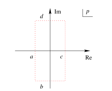
Figure 27: The contour for the analytic decomposition of $S_{n}(p)$.

Moving the segments $b$ and $d$ down and up to $-i\infty$ and $+i\infty$ respectively, their contributions to $S_{n}(p)$ vanish, allowing us to write

$$S_{n}(p)=G_{+}(p)-G_{-}(p)$$ (C.22)

where $G_{+}(p)$ is the contribution to (C.21) from $a$, and $G_{-}(p)$ is (minus) the contribution from $c$, and these two functions do indeed decay in the right and left half-planes, respectively. Changing integration variable to $t\equiv p^{\prime}/i$ and using (C.13) for $S_{n}(p)$, (C.20) becomes

$$a_{n}(p)=\frac{(-1)^{n}}{2\pi^{2}}\frac{\Gamma(2{-}n{+}ng{+}2p)}{\Gamma(n{-}1{-}ng{+}2p)}\,\int_{-\infty}^{\infty}\!\frac{\Gamma(n{-}1{-}ng{+}2it)\,\Gamma(n{-}1{-}ng{-}2it)\,R_{n}(it)}{(p{-}it)}\,dt~{},$$ (C.23)

and $a_{n}(p)$ has been determined uniquely in terms of the $a_{m}(p)$ with $m<n$. Since the first coefficient, $a_{1}(p)$, has already been fixed via the homogeneous equation and the asymptotic (C.3), this completes the proof that the power series (C.1) is uniquely determined by properties (i) – (v). Note that the question of the convergence of the series is at this stage moot. However, once the identification with the expansion of a spectral determinant has been made, this follows from standard properties of the solutions of ordinary differential equations.

Appendix D Derivation of the TBA equations and of the NLIE

In this appendix we describe how to turn certain functional relations into nonlinear integral equations. We also indicate how the equations encode the effective central charges of the associated integrable models.

D.1 TBA equations from truncated fusion hierarchies

Finite sets of functional equations such as the T-system (3.63) – or equivalently (5.45) – can be transformed into sets of nonlinear integral equations of the form known in the integrable model community as thermodynamic Bethe ansatz (TBA) equations [152]. Recall that the T-system (3.63) is the following set of $h{-}1$ coupled functional equations

$$\quad t^{(m)}(\omega^{-1}E)t^{(m)}(\omega E)=1+\prod_{j=1/2}^{(h-1)/2}\left(t^{(j)}(E)\right)^{G_{2j,2m}},~{}~{}~{}m=1/2,1,\dots,(h{-}1)/2$$ (D.1)

where $\omega=e^{2\pi i/h(M{+}1)}$ and $G$ is the incidence matrix of the $A_{h-1}$ Dynkin diagram. In fact the following arguments apply equally for any simply-laced Dynkin diagram, and so – in the spirit of [195, 196] – we shall give a slightly more general treatment here than is strictly needed for the differential equation application. Also, because we consider the more general situation we shall use the integrable model notation $T$ rather than $t$ and $s$ rather than $E$. We further streamline by setting $r=h{-}1$ and

$$T_{a}(s)=t^{(a/2)}(E)~{},\quad a=1\dots r$$ (D.2)

so that the T-system is

$$T_{a}(\omega^{-1}s)T_{a}(\omega s)=1+\prod_{b=1}^{r}\left(T_{b}(s)\right)^{G_{ab}},\quad a=1\dots r.$$ (D.3)

In the more general cases, $a$ and $b$ label nodes on the Dynkin diagram described by $G_{ab}$ , and $r$ is its rank.

The first step towards the TBA is to introduce the Y-functions, defined by

$$Y_{a}(s)=\prod_{b=1}^{r}T_{b}(s)^{G_{ab}}~{},\quad a=1\dots r.$$ (D.4)

Clearly, (D.3) implies

$$T_{b}(\omega^{-1}s)T_{b}(\omega s)=1+Y_{b}(s)$$ (D.5)

and a suitable product over $b$ results in the set of equations

$$Y_{a}(\omega s)Y_{a}(\omega^{-1}s)=\prod_{b=1}^{r}(1+Y_{b}(s))^{G_{ab}}\,,$$ (D.6)

called a Y-system. Equivalently, on setting $s=e^{\theta/\mu}$ with $\mu=(M+1)/hM$, we have

$$Y_{a}(\theta+i{\textstyle\frac{\pi}{h}})Y_{a}(\theta-i{\textstyle\frac{\pi}{h}})=\prod_{b=1}^{h-1}\left(1+Y_{b}(\theta)\right)^{G_{ab}}\,.$$ (D.7)

These coincide with the Y-systems of Al.B. Zamolodchikov [195], which for the $A_{h-1}$ cases encode the finite size effects of certain integrable quantum field theories with ${\mathbb{Z}}_{h}$ symmetry. (We shall comment on the relationship between these models and the continuum limit of the twisted six-vertex model at the relevant values of $\phi$ and $\eta$ at the end of this subsection.)

Since in our cases $T$ and $Y$ are entire functions of $s$, they are $2\pi i\mu=2\pi i(h{+}2)/h$ -periodic functions of $\theta$. In fact, given the symmetry $Y_{a}=Y_{h-a}$, this periodicity also follows from the Y-system (D.7); see [195, 197, 198] for more details.

Next, the Y-system is transformed into a set of integral equations by introducing the ‘pseudoenergies’

$$\varepsilon_{a}(\theta)=\ln Y_{a}(\theta)~{},$$ (D.8)

which as a result of (D.7) satisfy

$$\varepsilon_{a}(\theta+i{\textstyle\frac{\pi}{h}})+\varepsilon_{a}(\theta-i{\textstyle\frac{\pi}{h}})-\sum_{b=1}^{r}G_{ab}\varepsilon_{b}(\theta)=\sum_{b=1}^{r}G_{ab}\,L_{b}(\theta)$$ (D.9)

with

$$L_{a}(\theta)=\ln(1{+}e^{-\varepsilon_{a}(\theta)})~{}.$$ (D.10)

Equation (D.9) has many solutions, and to pin things down some more information about the properties of the functions involved is required. We shall need the following. Since the functions $t^{(a/2)}(s)$ are entire and hence regular at $E=0$, the $Y_{a}(\theta)$ approach constant values as $\theta\rightarrow-\infty$ . These constants solve the stationary ($\theta$-independent) version of (D.7); as will be justified shortly, the particular solution relevant here has all its components positive:

$${\cal Y}_{a}=\lim_{\theta\rightarrow-\infty}e^{\varepsilon_{a}(\theta)}={\sin({\textstyle\frac{a\pi}{h+2}})\sin({\textstyle\frac{(a+2)\pi}{h+2}})\over\sin^{2}({\textstyle\frac{\pi}{h+2}})}~{}.$$ (D.11)

On the other hand, as $|s|\to\infty$ with $-\pi+\delta<\arg(s)<\pi-\delta$ (where $\delta$ is an arbitrarily-small positive number), the leading asymptotics of the $\ln(t^{(m)}(s))$, and hence also of the $\ln(Y_{a}(s))$, are proportional to $s^{\mu}$ . Thus, as $\Re e\,\theta\to+\infty$ in any strip $|\Im m\,\theta|<\pi(h{+}2)/h-\delta$, the pseudoenergies behave as

$$\varepsilon_{a}(\theta)\sim m_{a}L\,e^{\theta}\,,$$ (D.12)

with, in fact, exponentially-small corrections. A consideration of (D.9) at large real values of $\theta$, where the right-hand side vanishes, shows that the constants $m_{a}L$ are proportional to the components of the Perron-Frobenius eigenvector of $G$. For the $A_{h-1}$ case of prime interest here, we can write these components as

$$m_{a}L={\textstyle\frac{b_{0}}{2}}\sin({\textstyle\frac{\pi a}{h}})~{},\quad b_{0}\in{\mathbb{R}}\,.$$ (D.13)

Finally, for the solution of (D.9) that we require here – the ground state eigenvalue of the integrable model, or equivalently the quantum-mechanical spectral determinant – the zeros of the $t^{(a/2)}(s)$ all lie on the negative $s$ axis. This means that the Y-functions do not vanish on the real $\theta$ axis, which when combined with (D.12) justifies the choice of the solution (D.11) of the stationary Y-system. It also implies that the functions

$$f_{a}(\theta)=\varepsilon_{a}(\theta)-m_{a}L\,e^{\theta}$$ (D.14)

are bounded in the ‘analyticity strip’ $|\Im m(\theta)|<\pi/h$ and satisfy the relation

$$f_{a}(\theta+i{\textstyle\frac{\pi}{h}})+f_{a}(\theta-i{\textstyle\frac{\pi}{h}})-\sum_{b=1}^{r}G_{ab}f_{b}(\theta)=\sum_{b=1}^{r}G_{ab}\,L_{b}(\theta)\,.$$ (D.15)

Taking an ($\epsilon$-regularised) Fourier transform

$$\widetilde{f}(k)={\cal F}[f(\theta)]=\lim_{\epsilon\rightarrow 0^{+}}\int_{-\infty}^{\infty}d\theta\,f(\theta)e^{-ik\theta+\epsilon\theta}$$ (D.16)

of both sides of (D.15),

$$\sum_{b=1}^{r}(2\,\delta_{ab}\cosh({\textstyle\frac{\pi k}{h}})-G_{ab})\,\widetilde{f}_{b}(k)=\sum_{b=1}^{r}G_{ab}\,\widetilde{L}_{b}(k)\,.$$ (D.17)

Solving for $\widetilde{f}_{a}(k)$ and transforming back to $\theta$-space yields the equations

$$\varepsilon_{a}(\theta)=m_{a}Le^{\theta}-{1\over 2\pi}\sum_{b=1}^{r}\int_{-\infty}^{\infty}\,\phi_{ab}(\theta-\theta^{\prime})L_{b}(\theta^{\prime})\,d\theta^{\prime}$$ (D.18)

with

$$\widetilde{\phi}_{ab}(k)=-2\pi\sum_{c=1}^{r}\left(2\,\delta_{ac}\cosh({\textstyle\frac{\pi k}{h}})-G_{ac}\right)^{-1}G_{cb}~{}.$$ (D.19)

The inverse Fourier transforms of the kernels $\widetilde{\phi}_{ab}(k)$ can be found exactly in terms of elementary functions, and the results written as

$$\phi_{ab}(\theta)=-i\frac{d}{d\theta}\ln S_{ab}(\theta)\,,$$ (D.20)

where

$$S_{ab}(\theta)=\prod_{x\in A_{ab}}\{x\}~{},\qquad a,b=1\dots r\,.$$ (D.21)

The integer-valued index set $A_{ab}$ can be characterised via the Weyl group of the related Lie algebra, and

$$\{x\}=(x{-}1)(x{+}1)\,~{}~{}~{},~{}~{}~{}(x)={\sinh({\textstyle\frac{\theta}{2}}{+}i{\textstyle\frac{\pi x}{2h}})\over\sinh({\textstyle\frac{\theta}{2}}{-}i{\textstyle\frac{\pi x}{2h}})}~{}.$$ (D.22)

For $A_{h-1}$ the explicit formula is

$$S_{ab}(\theta)=\prod_{|a-b|+1\atop{\rm step~{}2}}^{{}\atop a+b-1}\{x\}~{},\qquad a,b=1\dots r\,.$$ (D.23)

For the other cases see, for example, [199, 200]; for their relation with the Fourier transforms (D.19), see [195, 196].

Nonlinear integral equations of the form (D.18) also arise in the framework of the thermodynamic Bethe ansatz [152, 201] method for finding the ground-state energies of massive relativistic integrable field theories in $1+1$ dimensions, and hence they are often called TBA equations. In this picture $L$ should be interpreted as the circumference of the infinite cylinder on which the theory is defined, and $S_{ab}(\theta)$ are the two-particle S-matrix elements describing the factorised scattering of $r$ particles of relative masses $m_{a}$. Strictly speaking, the equations just derived correspond to an ultraviolet limit of these TBA equations, in which the overall mass scale is taken to zero.

Once the $\varepsilon_{a}(\theta)$ and hence the $Y_{a}(\theta)$ have been found via (D.18), it remains to recover the T-functions. This can be done using much the same reasoning as led to the TBA equation, starting this time from (D.5). Dividing through by $Y_{a}(s)$, using (D.4) and taking logs,

$$\ln T_{a}(\theta+i{\textstyle\frac{\pi}{h}})+\ln T_{a}(\theta-i{\textstyle\frac{\pi}{h}})-\sum_{b=1}^{r}G_{ab}\ln T_{b}(\theta)=L_{a}(\theta)\,.$$ (D.24)

From (D.11) and (D.5), the functions $\ln T_{a}(\theta)-m_{a}L\,e^{\theta}/(2\cos(\pi/h))$ are bounded in the same analyticity strip as the $f_{a}(\theta)$ above, and can likewise be found by a Fourier transformation. The final result is

$$\ln T_{a}(\theta)=\frac{m_{a}L}{2\cos(\pi/h)}\,e^{\theta}-{1\over 2\pi}\sum_{b=1}^{r}\int_{-\infty}^{\infty}\,\psi_{ab}(\theta-\theta^{\prime})L_{b}(\theta^{\prime})\,d\theta^{\prime}$$ (D.25)

where the Fourier transform of the kernel $\psi_{ab}(\theta)$ is

$$\widetilde{\psi}_{ab}(k)=-2\pi\left(2\,\delta_{ab}\cosh({\textstyle\frac{\pi k}{h}})-G_{ab}\right)^{-1}.$$ (D.26)

Again, the inverse transform can be performed, to find that $\psi_{ab}(\theta)$ is defined as $\phi_{ab}(\theta)$, save for the replacement of the blocks $\{x\}$ by $(x)$ in (D.21). However, as explained in section E.1 below, for spectral applications one can often get away without calculating the $T_{a}$ explicitly [1].

It is also interesting to extract the ground state energy of the spin chain, or of the corresponding quantum field theory. It might be tempting to use (3.19) for this purpose, but one has to be careful as the continuum limit involves an infinite shift of the $\theta$-like variable $\nu$ in (3.19). This provides some intuition for the fact that the universal part of the continuum ground-state energy is to be found in the large-$\theta$ asymptotic of the fundamental transfer matrix, $T_{1}(\theta)$ in current notations.

The relevant asymptotic expansion has the form [30, 202]

$$\ln T_{1}(\theta)-\frac{m_{1}L}{2\cos(\pi/h)}\,e^{\theta}\sim-\sum_{n=1}^{\infty}C_{n}I^{\rm vac}_{2n{-}1}\,e^{(1{-}2n)\theta}$$ (D.27)

where the numbers $I^{\rm vac}_{2n-1}$ are the eigenvalues of the local conserved charges of the system on a cylinder of circumference $L$. The first of these, $I_{1}$, gives the ground state energy; and from the results of [30, 202],

$$\ln T_{1}(\theta)-\frac{m_{1}L}{2\cos(\pi/h)}\,e^{\theta}\sim-\frac{4\sin(\pi/h)}{m_{1}}\,I^{\rm vac}_{1}\,e^{-\theta}-\dots~{}.$$ (D.28)

This asymptotic also follows from (D.24). Let $q^{(\sigma)}_{a}$ be an orthonormal set of eigenvectors of $G_{ab}$, where $\sigma$ runs over the exponents of $G$, so that

$$\sum_{b=1}^{r}G_{ab}\,q^{(\sigma)}_{b}=2\cos(\pi\sigma/h)\,q^{(\sigma)}_{a}\quad,\quad\sum_{\sigma}q_{a}^{(\sigma)}q_{b}^{(\sigma)}=\delta_{ab}\,.$$ (D.29)

Then

$$\widetilde{\psi}_{ab}(k)=-\pi\sum_{\sigma}\frac{q_{a}^{(\sigma)}q_{b}^{(\sigma)}}{\cosh(\pi k/h)-\cos(\pi\sigma/h)}$$ (D.30)

and is easily seen to have poles at $k=(\pm\sigma+2hn)i$, $n\in{\mathbb{Z}}$ . For large $\theta$ the inverse Fourier transform yielding $\psi_{ab}(\theta)$ can be expanded over the residues of these poles, the leading term coming from the pole nearest to the real axis:

$$\psi_{ab}(\theta) = \frac{1}{2\pi}\int_{-\infty}^{\infty}dk\,\widetilde{\psi}(k)e^{ik\theta}$$ (D.31)

$$= \frac{-h\,}{\sin(\pi/h)}\,q^{(1)}_{a}q^{(1)}_{b}\,e^{-\theta}+\dots~{}.$$

For the $A_{r}$ case relevant for comparison with the expansion (D.27), the normalised eigenvector has components $q^{(1)}_{a}=\sqrt{\frac{2}{h}}\,\sin(\pi a/h)$. Substituting (D.31) into the integral formula (D.25) and swapping sums with integrals gives an asymptotic expansion which matches (D.27), and begins

$$\qquad\ln T_{1}(\theta)-\frac{m_{1}L}{2\cos(\pi/h)}\,e^{\theta}=\frac{1}{\pi}\sum_{b=1}^{r}\int_{-\infty}^{\infty}\sin(\pi b/h)\,e^{-\theta+\theta^{\prime}}L_{b}(\theta^{\prime})\,d\theta^{\prime}+\dots~{}.$$ (D.32)

Comparing leading terms,

$$I^{\rm vac}_{1}\equiv E_{0}(L) = -\frac{1}{4\pi}\sum_{a=1}^{r}\int_{-\infty}^{\infty}m_{1}\frac{\sin(\pi a/h)}{\sin(\pi/h)}e^{\theta}L_{a}(\theta)\,d\theta$$ (D.33)

$$= -\frac{1}{4\pi}\sum_{a=1}^{r}\int_{-\infty}^{\infty}m_{a}e^{\theta}L_{a}(\theta)\,d\theta$$

where $L_{a}(\theta)=\ln(1+e^{-\varepsilon(\theta)})$ and $\varepsilon(\theta)$ solves (D.18). Recalling that $c_{\rm eff}$ was defined via

$$E_{0}(L)=F(L)=-\frac{\pi c_{\rm eff}}{6L}\,,$$ (D.34)

we see that (D.33) is equivalent to

$$c_{\rm eff}=\frac{3}{2\pi^{2}}\sum_{a=1}^{r}\int_{-\infty}^{\infty}d\theta\,m_{a}L\,e^{\theta}L_{a}(\theta)\,.$$ (D.35)

Even though $\varepsilon(\theta)$ cannot be found in closed form, it turns out that the integral in (D.35) can be calculated exactly as a sum of Rogers dilogarithm functions

$${\cal L}(x)=-{1\over 2}\int_{0}^{x}dy\left[{\ln y\over 1-y}+{\ln(1-y)\over y}\right]~{}.$$ (D.36)

(For more about sum rules for Rogers dilogarithm see [203].) For our model, the final result is

$$c_{\rm eff} = {3\over\pi^{2}}\sum_{a=1}^{r}{\cal L}\left({1\over 1+{\cal Y}_{a}}\right)={3\over\pi^{2}}\sum_{a=1}^{r}{\cal L}\left({\sin^{2}({\textstyle\frac{\pi}{h+2}})\over\sin^{2}(\pi{\textstyle\frac{a+1}{h+2}})}\right)$$ (D.37)

$$= {h-1\over h+2}={2M-1\over 2M+2}\quad,\quad(h=2M)~{},$$

which is exactly half the central charge for the ${\mathbb{Z}}_{h}$ parafermion models [204]. How does this compare with the continuum limit of the twisted six-vertex model? As mentioned before the untwisted six-vertex model is equivalent, in its continuum limit, to the theory of a free compactified boson with central charge $c_{\rm eff}^{6V}=1$. For the twisted variant of the six-vertex model we have instead

$$c_{\rm eff}^{T6V}=1-\frac{6\phi^{2}}{\pi(\pi-2\eta)}.$$ (D.38)

Inserting the relations

$$\eta={\pi\over 2}{M\over M+1}~{},~{}~{}~{}~{}\phi={\pi\over 2M+2}$$ (D.39)

we find

$$c_{\rm eff}^{T6V}={2M-1\over 2M+2}~{},$$ (D.40)

which is the result quoted in (D.37). The factor of two discrepancy with the parafermionic central charge is, for $h$ odd, simply due to a double counting that can be avoided via a folding procedure that identifies conjugate nodes $j\leftrightarrow h-j$ in the related $A_{h-1}$ Dynkin diagram. A slightly more subtle folding phenomena is at work in the $h$ even case too [1].

D.2 NLIEs from Bethe ansatz systems

The TBA method relies on the truncation of the fusion hierarchy, and so can only work at rational values of $\eta/\pi$ or $M$. In addition the resulting equations depend in a complicated way on the arithmetic properties of these numbers. However, there is another approach which works more generally. Employing ideas developed in [205, 27, 28, 31, 5], the Bethe ansatz equations associated with a TQ relation of the type discussed here can be transformed into a single nonlinear integral equation. Starting with the TQ relation (5.14), set $E=E_{k}$ and invoke the entirety of $C(E,l)$ and $D(E,l)$ to obtain

$$\omega^{2l+1}\frac{D(\omega^{2}E_{k},l)}{D(\omega^{-2}E_{k},l)}+1=0\quad,\quad k=1,2,\dots~{}.$$ (D.41)

Replacing $D(E,l)$ with its Hadamard factorisation (5.22), valid for $M>1$, the Bethe ansatz equations for the eigenvalues of $D(E,l)$ are recovered:

$$\prod_{j=1}^{\infty}\left(\frac{E_{j}-\omega^{2}E_{k}}{E_{j}-\omega^{-2}E_{k}}\right)=-\omega^{2l+1}\quad,\quad k=1\dots~{}.$$ (D.42)

Setting

$$a(E)=\omega^{2l{+}1}\frac{D(\omega^{2}E,l)}{D(\omega^{-2}E,l)}=\omega^{2l{+}1}\prod_{j=1}^{\infty}\left(\frac{E_{j}-\omega^{2}E}{E_{j}-\omega^{-2}E}\right)~{},$$ (D.43)

the Bethe ansatz equations are rephrased as conditions on the function $a(E)$:

$$a(E_{k})+1=0\quad,\quad k=1,2,\dots~{}.$$ (D.44)

In fact, it follows from the TQ relation that the zeros of $a(E)+1$ are precisely the zeros of $D(E)$, the Bethe roots $E_{k}$, together with the zeros of $T(E)$. For simplicity, we consider the ground state situation, for which all the $E_{k}$ are real and positive, and all the zeros of $T(E)$ are real and negative. We begin by taking the logarithm of (D.43)

$$\ln a(E)=\frac{i\pi(2l{+}1)}{M{+}1}+\sum_{k=1}^{\infty}F(E/E_{k})~{},$$ (D.45)

where $F(E)=\ln[(1-\omega^{2}E)/(1-\omega^{-2}E)]$ . The logarithmic derivative $\partial_{E}\ln(1+a(E))$ has a simple pole at each eigenvalue $E_{k}$. Applying Cauchy’s theorem, the infinite sum in (D.45) can be replaced by a contour integral, the contour encircling the points $E_{k}$ in an anticlockwise direction, while avoiding all other singularities of $\ln(1+a(E))$. Given our assumptions about the locations of the zeros of $D(E)$ and $T(E)$, a suitable contour $\cal C$ runs from $+\infty$ to $0$ above the real axis, encircles the origin then returns to $\infty$ below the real axis. With this in mind (D.45) becomes

$$\ln a(E)=\frac{i\pi(2l{+}1)}{M{+}1}+\int_{\cal C}\frac{dE^{\prime}}{2\pi i}\,F(E/E^{\prime})\,\partial_{E^{\prime}}\ln(1+a(E^{\prime}))\,.$$ (D.46)

We change variables via $E=\exp(2M\theta/(M{+}1))$ and define (with a mild abuse of notation) $\ln a(\theta)\equiv\ln a(e^{2M\theta/(M+1)})\,$. Integrating by parts we have

$$\ln a(\theta) = \frac{i\pi(2l{+}1)}{M{+}1}-\int_{{\cal C}_{1}}d\theta^{\prime}\,\partial_{\theta^{\prime}}R(\theta-\theta^{\prime})\ln(1+a(\theta^{\prime}))$$ (D.47)

$$\qquad\qquad\qquad{}+\int_{{\cal C}_{2}}d\theta^{\prime}\,\partial_{\theta^{\prime}}R(\theta-\theta^{\prime})\ln(1+a(\theta^{\prime}))~{},$$

where

$$R(\theta)~{}=~{}\frac{i}{2\pi}\,\partial_{\theta}F(e^{2M\theta/(M+1)})~{}.$$ (D.48)

The new integration contours ${\cal C}_{1}$ and ${\cal C}_{2}$ run from $-\infty$ to $\infty$ just below and just above the real axis respectively. Using the property $[a(\theta)]^{*}=a(\theta^{*})^{-1}$, which follows from the Bethe ansatz equations, we rewrite the integrals in terms of integrations along the real axis:

$$\ln a(\theta)-\int_{-\infty}^{\infty}d\theta^{\prime}R(\theta-\theta^{\prime})\ln a(\theta^{\prime}) = \frac{i\pi(2l{+}1)}{M{+}1}$$ (D.49)

$$\hskip-65.44142pt{}-2i\int_{-\infty}^{\infty}d\theta^{\prime}R(\theta{-}\theta^{\prime})\Im m\ln(1+a(\theta^{\prime}{-}i0))~{}.$$

It is then a simple matter to solve this equation using Fourier transforms. Using the notation $\widetilde{f}(k)$ and ${\cal F}[f(\theta)](k))$ introduced earlier, the Fourier-transformed equation is

$$(1-\widetilde{R}(k))\,{\cal F}[\ln a](k)=-\frac{2\pi^{2}(2l{+}1)}{M{+}1}\delta(k)-2i\widetilde{R}(k)\,\Im m\,{\cal F}[\ln(1+a)](k)~{}.$$ (D.50)

We apply $(1-\widetilde{R}(k))^{-1}$ to both sides, then take the inverse Fourier transform to find

$$\ln a(\theta) = \frac{i\pi(2l{+}1)}{M{+}1}{\cal F}^{-1}[(1-\widetilde{R}(k))^{-1}](0)+imL\,e^{\theta}$$ (D.51)

$$\hskip 28.45274pt{}-2i\int_{-\infty}^{\infty}d\theta^{\prime}\,\varphi(\theta-(\theta^{\prime}-i0))\Im m\,\ln(1+a(\theta^{\prime}-i0))\,,$$

where

$$\varphi(\theta)={\cal F}^{-1}\,[\,(1-{\widetilde{R}}(k))^{-1}{\widetilde{R}}(k)\,](\theta)~{},$$ (D.52)

and $mL$ is a real constant which arises from a zero mode and can be traced to the pole in $(1-{\widetilde{R}}(k))^{-1}$ at $k=i$. It should be fixed by a consideration of the large-$\theta$ asymptotic of $\ln a(\theta)$. From the definition of $R(\theta)$ and the relations

$$i\partial_{\theta}\ln\frac{\sinh\sigma\theta+i\pi\tau}{\sinh\sigma\theta-i\pi\tau} = \frac{2\sigma\sin 2\pi\tau}{\cosh 2\sigma\theta-\cos 2\pi\tau}$$ (D.53)

$$\int_{-\infty}^{\infty}\frac{d\theta}{2\pi}\,e^{-ik\theta}\frac{2\sigma\sin 2\pi\tau}{\cosh 2\sigma\theta-\cos 2\pi\tau} = \frac{\sinh(1-2\tau)\frac{\pi k}{2\sigma}}{\sinh\frac{\pi k}{2\sigma}}$$ (D.54)

we obtain a compact expression for the kernel $\varphi(\theta)$:

$$\varphi(\theta)=\int\frac{dk}{2\pi}\,e^{ik\theta}\frac{\sinh\frac{\pi k(M-1)}{2M}}{2\sinh\frac{\pi\,k}{2M}\cosh\frac{\pi k}{2}}~{}.$$ (D.55)

Finally we rewrite the equation in terms of the integration contours ${\cal C}_{1}$ and ${\cal C}_{2}$:

$$\ln a(\theta) = i\pi(l+{\textstyle\frac{1}{2}})-imL\,e^{\theta}$$ (D.56)

$$+\int_{{\cal C}_{1}}d\theta^{\prime}\,\varphi(\theta{-}\theta^{\prime})\ln(1+a(\theta^{\prime}))-\int_{{\cal C}_{2}}d\theta^{\prime}\,\varphi(\theta{-}\theta^{\prime})\ln(1+a(\theta^{\prime})^{-1})~{}.$$

This equation holds for all $\theta$ within the strip $|\Im m\,\theta|<\min(\pi,\pi/M)$. A little extra care is required for larger $\Im m\,\theta$ as the kernel $\varphi(\theta)$ has poles at $\theta=\pm i\pi$ and $\pm i\pi/M$. If $M>1$, the correct analytic continuation for positive values of $\Im m\,\theta$ is given by the second determination [206]

$$\ln a(\theta) = -i(1-e^{-i\pi/M})mL\,e^{\theta}$$ (D.57)

$$+\int_{{\cal C}_{1}}d\theta^{\prime}\,\varphi_{II}(\theta{-}\theta^{\prime})\ln(1+a(\theta^{\prime}))-\int_{{\cal C}_{2}}d\theta^{\prime}\,\varphi_{II}(\theta{-}\theta^{\prime})\ln(1+a(\theta^{\prime})^{-1})~{},$$

where

$$\varphi_{II}(\theta)=\frac{2i\cos(\frac{\pi}{2M})\sinh{(\theta-\frac{i\pi}{2M}})}{\pi\left(\cosh(2\theta{-}{\textstyle\frac{i\pi}{M}})-\cos(\frac{\pi}{M})\right)}~{}.$$ (D.58)

This equation is valid for $\pi/M<\Im m\,\theta<\pi$, when $M>1$. A similar continuation can be performed for $M<1$. For a detailed discussion of the effect of this continuation on eigenvalue asymptotics, see [16].

The NLIE (D.56) first arose in [27] as the continuum limit of an equation describing the finite size effects of the six-vertex model. It also appears in relativistic integrable scattering field theory in $1+1$ dimensions, where it describes the finite size effects of the ultraviolet limit of the massive sine-Gordon model [205]. In the latter situation the kernel $\varphi(\theta)$ is related to the scalar factor of the sine-Gordon soliton-soliton scattering amplitude. In the field theory context, the effective central charge is given in terms of $\ln a(\theta)$ according to

$$c_{\rm eff}=\frac{3imL}{\pi^{2}}\left[\int_{{\cal C}_{1}}\,d\theta\,e^{\theta}\log(1+a(\theta^{\prime}))-\int_{{\cal C}_{2}}\,d\theta\,e^{\theta}\log(1+a^{-1}(\theta^{\prime}))\right].$$ (D.59)

This integral can be evaluated exactly, with the result

$$c_{\rm eff}=1-\frac{6(l+\frac{1}{2})^{2}}{M+1}~{},$$ (D.60)

which, given the relations $\beta^{2}=1/(M+1)$ and $p=(2l+1)/(4M+4)$, agrees perfectly with

$$c_{\rm eff}=c-24\Delta_{p}=1-24\,\frac{p^{2}}{\beta^{2}}~{}.$$ (D.61)

The above NLIE has been derived for the ground state, for which the Bethe roots $\{E_{k}\}$ are all real and positive. However, nonlinear integral equations of both TBA and NLIE types can be found even when some of the Bethe roots lie in the complex plane. See, for example, [31, 202, 206, 207, 208, 209].

Appendix E Calculating the spectrum of an ODE

We briefly describe how to calculate the spectrum of

$$\left[-\frac{d^{2}}{dx^{2}}+x^{2M}+\frac{l(l{+}1)}{x^{2}}-E\right]\,\psi(x)=0~{}.$$ (E.1)

using the nonlinear integral equations derived in appendix D.

E.1 TBA approach

When $M$ is an integer and $l(l+1)=0$ the spectrum encoded in the spectral determinant $D(E,l)$ can be determined from the fusion relations (5.45) using TBA equations. Recall the following relation obtained in section 3.7:

$$\frac{i}{2}T_{M/2}(E)=\frac{i}{2}C^{(M)}(v^{-1}E)=D(-E)\equiv D_{+}(-E)D_{-}(-E)~{}.$$ (E.2)

From this we see that the real positive zeros of $D(E)$ are precisely the real negative zeros of $T_{M/2}(E)$ or $C^{(M)}(E)$. We set

$$t^{(m)}(\theta+i\pi{\textstyle\frac{h+2}{2h}})\equiv T_{m}(-E)\quad,\quad h=2M~{}.$$ (E.3)

Then from

$$1+Y_{2m}(\theta+i{\textstyle\frac{\pi}{2}})=t^{(m)}(\theta+i\pi{\textstyle\frac{h+2}{2h}})t^{(m)}(\theta+i\pi{\textstyle\frac{h-2}{2h}})~{},$$ (E.4)

we see that the eigenvalues $\{E_{k}\}$ are those zeros of $1+Y_{M}(\theta)$ that lie along the line $\Im m\,\theta=\pi/2$.

The constants $m_{a}L=\frac{b_{0}}{2}\sin\frac{\pi a}{h}$ appearing in the TBA equations (D.18) must be tuned to match the asymptotic properties of the spectral determinants. The correct result is found by setting $b_{0}=2\cos(\pi/2M)\,a_{0}$ where $a_{0}$ was defined in (5.20).

A very simple iteration scheme can be used to solve the TBA equations (D.18) numerically. Starting from

$$\quad\varepsilon_{a}^{(n+1)}(\theta)=\alpha\varepsilon_{a}^{(n)}(\theta)+(1-\alpha)\left[m_{a}Le^{\theta}-{1\over 2\pi}\sum_{b=1}^{h-1}\int_{-\infty}^{\infty}\,\phi_{ab}(\theta-\theta^{\prime})L_{b}^{(n)}(\theta^{\prime}){d\theta^{\prime}\over 2\pi}\right]$$ (E.5)

with $\varepsilon^{(0)}_{a}(\theta)=m_{a}L\,e^{\theta}$ and $0<\alpha\leq 1$, (E.5) can be iterated until the desired accuracy ($\sim 10^{-14}$) is reached. Empirically the value $\alpha=0.5$ gives a very good rate of convergence usually in less than one hundred iterations. Once the functions $\varepsilon_{a}(\theta)$ are known numerically along the real axis, the TBA equations (D.18) provide an integral representation which can be used to reconstruct the functions $\varepsilon_{a}(\theta)$ and $Y_{a}(\theta)=\exp(\varepsilon_{a}(\theta))$ everywhere in the complex plane. The only point to watch is that the singularities of the kernels $\phi_{ab}$’s at $\pm\imath\pi/h$ and beyond necessitate the introduction of extra terms when the $\varepsilon_{a}$’s are continued beyond the strip $-\pi/h<\Im m\,\theta<\pi/h$.

E.2 NLIE approach

As mentioned above, the single nonlinear integral equation derived in appendix D.2 encodes the zeros of both the spectral determinants $C$ and $D$. The zeros of $1+a(E)$ on the positive real axis are the zeros of $D(E,l)$, while those on the negative real axis are the zeros of $C(E,l)$. Under the variable change $E=\exp(2M\theta/(M{+}1))$ the positive real axis of the complex $E$-plane becomes the real-$\theta$ axis. Therefore the eigenvalues encoded in $D(E,l)$ can be found by searching along the real axis for the zeros of $1+a(\theta)$. Similarly the eigenvalues of $C(E,l)$ can be found as zeros of $1+a(\theta)$ on the line $\Im m\,\theta=\pi(M{+1})/2M$. Before we can solve the NLIE (D.56) we must fix the constants $mL$. The large-$E$ asymptotics of $a(E)$ are

$$\ \log a(E)\sim\left\{\begin{array}[]{ll}-{\textstyle\frac{1}{2}}ib_{0}(1{-}e^{-i\pi/M})(E)^{\mu}&~{}\frac{2\pi}{M{+}1}<\arg(E)<2\pi-\frac{2\pi}{M{+}1}\\[7.0pt] -{\textstyle\frac{1}{2}}ib_{0}(E)^{\mu}&-\frac{2\pi}{M{+}1}<\arg(E)<\frac{2\pi}{M{+}1}\\[7.0pt] -{\textstyle\frac{1}{2}}ib_{0}(1{-}e^{i\pi/M})(E)^{\mu}&-2\pi+\frac{2\pi}{M{+}1}<\arg(E)<-\frac{2\pi}{M{+}1}\end{array}\right.~{},$$ (E.6)

where $b_{0}=2\cos(\frac{\pi}{2M})a_{0}$ as before. Above, by $(E)^{\mu}$ we imply $e^{i\mu\arg(E)}|E|^{\mu}$. Thus the first and third asymptotics coincide, as indeed they must since $a$ is a single-valued function of $E$. Given (5.27), we set $mL={\textstyle\frac{1}{2}}b_{0}v^{-\mu}$, though the factor of $v^{-\mu}$ is arbitrary and is purely to match the conventions of [4, 31].

The NLIE can also be solved by iteration and the function $a(\theta)$ constructed for all complex $\theta$ using the integral representations (D.56) or (D.57) as appropriate. Consequently the eigenvalues of the spectral determinants $D(E)$ and $C(E)$ can be calculated for all $M>0$ and $l$. This method is more generally applicable than the TBA approach simply because the NLIE depends on the parameters $M$ and $l$ in a continuous manner.

References

- [1] P. Dorey and R. Tateo, ‘Anharmonic oscillators, the thermodynamic Bethe ansatz and nonlinear integral equations’, J. Phys. A32 (1999) L419, [arXiv:hep-th/9812211].
- [2] V.V. Bazhanov, S.L. Lukyanov and A.B. Zamolodchikov, ‘Spectral determinants for Schrödinger equation and Q-operators of conformal field theory’, J. Statist. Phys 102 (2001) 567, [arXiv:hep-th/9812247].
- [3] J. Suzuki, ‘Anharmonic oscillators, spectral determinant and short exact sequence of ’, J. Phys. A32 (1999) L183, [arXiv:hep-th/9902053].
- [4] P. Dorey and R. Tateo, ‘On the relation between Stokes multipliers and the T-Q systems of conformal field theory’, Nucl. Phys. B563 (1999) 573, [arXiv:hep-th/9906219].
- [5] P. Dorey and R. Tateo, ‘Differential equations and integrable models: the case’, Nucl. Phys. B571 (2000) 583, [arXiv:hep-th/9910102].
- [6] J. Suzuki, ‘Functional relations in Stokes multipliers and solvable models related to ’, J. Phys. A33 (2000) 3507, [arXiv:hep-th/9910215].
- [7] J. Suzuki, ‘Functional relations in Stokes multipliers – fun with potential’, J. Stat. Phys. 102(3) (2001) 1029, [arXiv:quant-ph/0003066].
- [8] P. Dorey, C. Dunning and R. Tateo, ‘Differential equations for general Bethe ansatz systems’, J. Phys. A33 (2000) 8427, [arXiv:hep-th/0008039].
- [9] J. Suzuki, ‘Stokes multipliers, spectral determinants and T-Q relations’, RIMS Proceedings Kokyuroku Vol. 1221 (2001) 21, [arXiv:nlin-si/0009006].
- [10] P. Dorey, C. Dunning and R. Tateo, ‘Ordinary differential equations and integrable quantum field theories’, Proceedings of the Johns Hopkins workshop on current problems in particle theory 24, Budapest, 2000 (World Scientific 2001).
- [11] P. Dorey, C. Dunning and R. Tateo, ‘Spectral equivalences, Bethe Ansatz equations, and reality properties in -symmetric quantum mechanics’, J. Phys. A34 (2001) 5679, [arXiv:hep-th/0103051].
- [12] P. Dorey, C. Dunning and R. Tateo, ‘Supersymmetry and the spontaneous breakdown of symmetry’, J. Phys. A34 (2001) L391, [arXiv:hep-th/0104119].
- [13] P. Dorey, C. Dunning and R. Tateo, ‘Ordinary differential equations and integrable models’, Proc. Nonperturbative quantum effects 2000 PRHEP-tmr2000/034 [arXiv:hep-th/0010148].
- [14] V.V. Bazhanov, S.L. Lukyanov and A.B. Zamolodchikov, ‘Higher-level eigenvalues of Q-operators and Schrödinger equation’, Adv. Theor. Math. Phys. 7 (2004) 711, [arXiv:hep-th/0307108].
- [15] P. Dorey, J. Suzuki and R. Tateo, ‘Finite lattice Bethe ansatz systems and the Heun equation’, J. Phys. A37 (2004) 204, [arXiv:hep-th/0308053].
- [16] P. Dorey, A. Millican-Slater and R. Tateo, ‘Beyond the WKB approximation in -symmetric quantum mechanics’, J. Phys. A38 (2005) 1305, [arXiv:hep-th/0410013].
- [17] V.V. Bazhanov and V.V. Mangazeev, ‘Eight-vertex model and non-stationary Lamé equation’, J. Phys. A38 (2005) L145, [arXiv:hep-th/0411094].
- [18] V.V. Bazhanov and V.V. Mangazeev, ‘The eight-vertex model and Painlevé VI’, J. Phys. A39 (2006) 12235, [arXiv:hep-th/0602122].
- [19] P. Dorey, C. Dunning, D. Masoero, J. Suzuki and R. Tateo, ‘Pseudo-differential equations, and the Bethe ansatz for the classical Lie algebras’, Nucl. Phys. B772 (2007) 249, [arXiv:hep-th/0612298].
- [20] Y. Sibuya, ‘Global theory of a second-order linear ordinary differential equation with polynomial coefficient’, (Amsterdam: North-Holland 1975).
-
[21]
A. Voros, ‘Semi-classical correspondence and exact results: the case
of the spectra of homogeneous Schrödinger operators’,
J. Physique Lett. 43 (1982) L1;
— ‘The return of the quartic oscillator. The complex WKB method’, Ann. Inst. Henri Poincaré Vol XXXIX (1983) 211;
— ‘Exact resolution method for general 1D polynomial Schrödinger equation’, J. Phys. A32 (1999) 5993 (and Corrigendum J. Phys. A34 (2000) 5783), [arXiv:math-ph/9903045]. - [22] C.M. Bender and A. Turbiner, ‘Analytic continuation of eigenvalue problems’, Phys. Lett. A173 (1993) 442.
- [23] C.M. Bender and S. Boettcher, ‘Real spectra in non-hermitian Hamiltonians having symmetry’, Phys. Rev. Lett. 80 (1998) 5243, [arXiv:physics/9712001].
- [24] C.M. Bender, S. Boettcher and P.N. Meisinger, ‘ symmetric quantum mechanics’, J. Math. Phys. 40 (1999) 2201, [arXiv:quant-ph/9809072].
- [25] R.J. Baxter, ‘Partition function of the eight-vertex lattice model’, Ann. Phys. 70 (1972) 193.
-
[26]
R.J. Baxter, ‘Eight-vertex model in lattice statistics and
one-dimensional anisotropic Heisenberg chain;
1. Some fundamental eigenvectors’, Ann. Phys. 76 (1973) 1;
— ‘2. Equivalence to a generalized ice-type model’, Ann. Phys. 76 (1973) 25;
— ‘3. Eigenvectors of the transfer matrix and Hamiltonian’, Ann. Phys. 76 (1973) 48. - [27] A. Klümper and P.A. Pearce, ‘Analytical calculations of scaling dimensions: tricritical hard square and critical hard hexagons’, J. Stat. Phys. 64 (1991) 13.
- [28] A. Klümper, M.T. Batchelor and P.A. Pearce, ‘Central charges of the 6- and 19-vertex models with twisted boundary conditions’, J. Phys. A24 (1991) 3111.
-
[29]
P. Fendley, F. Lesage and H. Saleur, ‘Solving 1-D plasmas and 2-D
boundary problems using Jack polynomials and functional relations’,
J. Stat. Phys. 79 (1995) 799,
[arXiv:hep-th/9409176];
— ‘A unified framework for the Kondo problem and for an impurity in a Luttinger liquid’, J. Stat. Phys. 85 (1996) 211, [arXiv:cond-mat/9510055]. - [30] V.V. Bazhanov, S.L. Lukyanov and A.B. Zamolodchikov, ‘Integrable structure of conformal field theory, quantum KdV theory and thermodynamic Bethe ansatz’, Commun. Math. Phys. 177 (1996) 381, [arXiv:hep-th/9412229].
- [31] V.V. Bazhanov, S.L. Lukyanov and A.B. Zamolodchikov, ‘Integrable structure of conformal field theory II. Q-operator and DDV equation’, Commun. Math. Phys. 190 (1997) 247, [arXiv:hep-th/9604044].
- [32] V.V. Bazhanov, S.L. Lukyanov and A.B. Zamolodchikov, ‘Integrable structure of conformal field theory III. The Yang-Baxter relation’, Commun. Math. Phys. 200 (1999) 297, [arXiv:hep-th/9805008].
- [33] R.J. Baxter, ‘Exactly solved models in statistical mechanics’, (Academic Press 1982).
- [34] P. Di Francesco, P. Mathieu and D. Sénéchal, ‘Conformal field theory’, (Springer 1998).
- [35] T.D. Lee, ‘Some special examples in renormalizable field theory’, Phys. Rev. 95 (1954) 1329.
- [36] R.C. Brower, M.A. Furman and M. Moshe, ‘Critical exponents for the Reggeon quantum spin model’, Phys. Lett. B76 (1978) 213.
- [37] S.A. Denham, B.C. Harms and S.T. Jones, ‘Complex energy spectra in Reggeon quantum mechanics with cubic plus generalized quartic interactions’, Nucl. Phys. B188 (1981) 155.
- [38] E. Caliceti, S. Graffi and M. Maioli, ‘Perturbation theory of odd anharmonic oscillators’, Commun. Math. Phys. 75 (1980) 51.
- [39] V. Buslaev and V. Grecchi, ‘Equivalence of unstable anharmonic oscillators and double wells’, J. Phys. A26 (1993) 5541.
- [40] F. Kleefeld, ‘Non-Hermitian quantum theory and its holomorphic representation: introduction and some applications’, [arXiv:hep-th/0408028].
- [41] C. Bender, ‘Introduction to -symmetric quantum theory’, Contemporary Physics 46 (2005) 277, [arXiv:quant-ph/0501052].
- [42] M.E. Fisher, ‘Yang-Lee edge singularity and field theory’, Phys. Rev. Lett. 40 (1978) 1610.
- [43] J.L. Cardy, ‘Conformal invariance and the Yang-Lee edge singularity in two dimensions’, Phys. Rev. Lett. 54 (1985) 1354.
- [44] J.L. Cardy and G. Mussardo, ‘S matrix of the Yang-Lee edge singularity in two-dimensions’, Phys. Lett. B225 (1989) 275.
- [45] M. Reed and B. Simon, ‘Methods of modern mathematical physics, I & II’, (Academic Press 1972, 1975).
- [46] R.D. Richtmyer, ‘Principles of advanced mathematical physics I’, (Springer-Verlag 1978).
- [47] D. Bessis and J. Zinn-Justin, unpublished.
- [48] M. Kac, ‘On the average number of real roots of a random algebraic equation’, Bull. Amer. Math. Soc. 49 (1943) 314 and 938.
- [49] M. Kac, ‘On the average number of real roots of a random algebraic equation (II)’, Proc. London Math. Soc. (3) 50 (1949) 390.
- [50] A. Edelman and E. Kostlan, ‘How many zeros of a random polynomial are real?’, Bull. Amer. Math. Soc. 32 (1995) 1, [arXiv:math-CA/9501224]; Erratum: Bull. Amer. Math. Soc. 33 (1996) 325.
- [51] A.P. Aldous and Y.V. Fyodorov, ‘Real roots of random polynomials: universality close to accumulation points’, J. Phys. A37 (2004) 1231, [arXiv:math-ph/0309014].
- [52] F. Cannata, G. Junker and J. Trost, ‘Schrödinger operators with complex potential but real spectrum’, Phys. Lett. A246 (1998) 219, [arXiv:quant-ph/9805085].
- [53] A.A. Andrianov, F. Cannata, J.P. Dedonder and M.V. Ioffe, ‘SUSY quantum mechanics with complex superpotentials and real energy spectra’, Int. J. Mod. Phys. A14 (1999) 2675, [arXiv:quant-ph/9806019].
- [54] F.M. Fernandez, R. Guardiola, J. Ros and M. Znojil, ‘A family of complex potentials with real spectrum’, J. Phys. A32 (1999) 3105, [arXiv:quant-ph/9812026].
- [55] C.M. Bender and G.V. Dunne, ‘Large-order perturbation theory for a non-Hermitian -symmetric Hamiltonian’, J. Math. Phys. 40 (1999) 4616, [arXiv:quant-ph/9812039].
- [56] E. Delabaere and F. Pham, ‘Eigenvalues of complex Hamiltonians with -symmetry. I’, Phys. Lett. A250 (1998) 25.
- [57] C.M. Bender, S. Boettcher, H.F. Jones and V.M. Savage, ‘Complex square well – a new exactly solvable quantum mechanical model’, J. Phys. A32 (1999) 6771, [arXiv:quant-ph/9906057].
- [58] B. Bagchi and R. Roychoudhury, ‘A new -symmetric complex Hamiltonian with a real spectrum’, J. Phys A33 (2000) L1, [arXiv:quant-ph/9911104].
- [59] G.A. Mezincescu, ‘Some properties of eigenvalues and eigenfunctions of the cubic oscillator with imaginary coupling constant’, J. Phys. A33 (2000) 4911, [arXiv:quant-ph/0002056].
- [60] E. Delabaere and D. Trinh, ‘Spectral analysis of the complex cubic oscillator’, J. Phys. A33 (2000) 8771.
- [61] B. Bagchi, F. Cannata and C. Quesne, ‘-symmetric sextic potentials’, Phys. Lett. A269 (2000) 79, [arXiv:quant-ph/0003085].
- [62] A. Khare and B.P. Mandal, ‘Non-Hermitian and non-PT invariant potentials with real QES eigenvalues’, [arXiv:quant-ph/0004019].
- [63] A. Khare and B.P. Mandal, ‘A -invariant potential with complex QES eigenvalues’, Phys. Lett. A272 (2000) 53, [arXiv:quant-ph/0006126].
- [64] B. Bagchi and C. Quesne, ‘ as a complex Lie algebra and the associated non-Hermitian Hamiltonians with real eigenvalues’, Phys. Lett. A273 (2000) 285, [arXiv:math-ph/0008020].
- [65] K.C. Shin, ‘On the eigenproblems of -symmetric oscillators’, J. Math. Phys. 42 (2001) 2513.
- [66] F. Cannata, M. Ioffe, R. Roychoudhury, P. Roy, ‘A New Class of -symmetric Hamiltonians with Real Spectra’, Phys. Lett. A281 (2001) 305, [arXiv:quant-ph/0011089].
- [67] C.M. Bender, G.V. Dunne, P.N. Meisinger and M. Simsek, ‘Quantum complex Hénon-Heiles potentials’, Phys. Lett. A281 (2001) 311, [arXiv:quant-ph/0101095].
- [68] C.M. Bender, M. Berry, P.N. Meisinger, Van M. Savage and M. Simsek, ‘Complex WKB analysis of energy-level degeneracies of non-Hermitian Hamiltonians’, J. Phys. A 34 (2001) L31.
- [69] B. Bagchi, S. Mallik and C. Quesne, ‘Generating complex potentials with real eigenvalues in supersymmetric quantum mechanics’, Int. J. Mod. Phys. A16 (2001) 2859, [arXiv:quant-ph/0102093].
- [70] C.M. Bender and Q. Wang, ‘Comment on a recent paper by Mezincescu’, J. Phys. A34 (2001) 3325.
- [71] G.A. Mezincescu, ‘The operator on (reply to Comment by Bender and Wang)’, J. Phys. A34 (2001) 3329.
- [72] C.R. Handy, ‘Generating converging eigenenergy bounds for the discrete states of the non-Hermitian potential’, J. Phys. A34 (2001) L271.
- [73] C.R. Handy, ‘Generating converging bounds to the (complex) discrete states of the Hamiltonian’, J. Phys. A34 (2001) 5065, [arXiv:math-ph/0104036].
- [74] C.R. Handy and X.Q. Wang, ‘Extension of a spectral bounding method to complex rotated Hamiltonians, with application to ’, J. Phys. A34 (2001) 8297, [arXiv:math-ph/0105019].
- [75] Z. Yan and C.R. Handy, ‘Extension of a spectral bounding method to the -invariant states of the non-Hermitian potential’, J. Phys. A34 (2001) 9907.
- [76] C.W. Bernard and V.M. Savage, ‘Numerical simulations of -symmetric quantum field theories’, Phys. Rev. D64 (2001) 085010, [arXiv:hep-lat/0106009].
- [77] A. Mostafazadeh, ‘Pseudo-Hermiticity versus symmetry. The necessary condition for the reality of the spectrum’, J. Math. Phys. 43 (2002) 205, [arXiv:math-ph/0107001].
- [78] Z. Ahmed, ‘Pseudo-Hermiticity of Hamiltonians under imaginary shift of the coordinate. Real spectrum of complex potentials’, Phys. Lett. A290 (2001) 19, [arXiv:quant-ph/0108016].
- [79] C.M. Bender, S. Boettcher, H.F. Jones, P. Meisinger and M. Simsek, ‘Bound states of non-Hermitian quantum field theories’, Phys. Lett. A291 (2001) 197, [arXiv:hep-th/0108057].
- [80] M. Znojil and M. Tater, ‘Complex Calogero model with real energies’, J. Phys. A34 (2001) 1793, [arXiv:quant-ph/0010087].
- [81] A. Mostafazadeh, ‘Pseudo-Hermiticity versus -Symmetry II: a complete characterization of non-Hermitian Hamiltonians with a real spectrum’, J. Math. Phys. 43 (2002) 2814, [arXiv:math-ph/0110016].
- [82] M. Znojil and G. Levai, ‘Spontaneous breakdown of PT symmetry in the solvable square-well model’, Mod. Phys. Lett. A16 (2001) 2273, [arXiv:hep-th/0111213].
- [83] C.K. Mondal, K. Maji and S.P. Bhattacharyya, ‘On the eigenvalues and dynamics of non-Hermitian symmetric Hamiltonians in finite basis spaces’, Phys. Lett. A291 (2001) 203.
- [84] A. Mostafazadeh, ‘Pseudo-Hermiticity versus -symmetry III: equivalence of pseudo-Hermiticity and the presence of antilinear symmetries’, J. Math. Phys. 43 (2002) 3944, [arXiv:math-ph/0203005].
- [85] S. Albeverio, S.M. Fei and P. Kurasov, ‘Point interactions: -Hermiticity and reality of the spectrum’, Lett. Math. Phys. 59 (2002) 227.
- [86] Z. Ahmed, ‘Pseudo-hermiticity of Hamiltonians under gauge-like transformation. Real spectrum of non-Hermitian Hamiltonians’, Phys. Lett. A294 (2002) 287.
- [87] C.M. Bender, M.V. Berry and A. Mandilara, ‘Generalized symmetry and real spectra’, J. Phys. A35 (2002) L467.
- [88] T.V. Fityo, ‘A new class of non-Hermitian Hamiltonians with real spectra’, J. Phys. A35 (2002) 5893.
- [89] K.C. Shin, ‘The potential generates real eigenvalues only, under symmetric rapid decay conditions’, J. Math. Phys. 46 (2005) 082110, [arXiv:hep-ph/0207251].
- [90] A. Mostafazadeh, ‘Pseudo-Hermiticity and generalized PT- and CPT-symmetries’, J. Math. Phys. 44 (2003) 974, [arXiv:math-ph/0209018].
- [91] S. Weigert, ‘-symmetry and its spontaneous breakdown explained by anti-linearity’, J. Opt B. 5 (2003) S416, [arXiv:quant-ph/0209054].
- [92] K.C. Shin, ‘On the reality of the eigenvalues for a class of -symmetric oscillators’, Commun. Math. Phys. 229 (2002) 543, [arXiv:math-ph/0201013].
- [93] A. Jannussis, G. Brodimas, S. Baskoutas and A. Leodaris, ‘Non-Hermitian harmonic oscillator with discrete complex or real spectrum for non-unitary squeeze operators’, J. Phys. A36 (2003) 2507.
- [94] O. Yesiltas, M. Simsek, R. Sever and C. Tezcan, ‘Exponential type complex and non-Hermitian potentials in -symmetric quantum mechanics’, Phys. Scripta 67 (2003) 472, [arXiv:hep-ph/0303014].
- [95] A. Mostafazadeh, ‘Exact -Symmetry is equivalent to Hermiticity’, J. Phys. A36 (2003) 7081, [arXiv:quant-ph/0304080].
- [96] Z. Ahmed, ‘Pseudo-reality and pseudo-adjointness of Hamiltonians’, [arXiv:quant-ph/0306093].
- [97] C.S. Jia, L.Z. Yi, S. Yu, J.Y. Liu and L.T. Sun, ‘New solvable pseudo-Hermitian potential models with real spectra’, Mod. Phys. Lett. A18 (2003) 1247.
- [98] O. Rosas-Ortiz and R. Munoz, ‘Non-hermitian SUSY hydrogen-like Hamiltonians with real spectra’, J. Phys. A36 (2003) 8497.
- [99] B. Basu-Mallick, T. Bhattacharyya, A. Kundu and B.P. Mandal, ‘Bound and scattering states of extended Calogero model with an additional invariant interaction’, Czech. J. Phys. 54 (2004) 5, [arXiv:hep-th/0309136].
- [100] P. Dorey, C. Dunning and R. Tateo, ‘A reality proof in -symmetric quantum mechanics’, Czech. J. Phys. 54 (2004) 35, [arXiv:hep-th/0309209].
- [101] P.K. Ghosh and K.S. Gupta, ‘On the real spectra of Calogero model with complex coupling’, Phys. Lett. A323 (2004) 29, [arXiv:hep-th/0310276].
- [102] A. Sinha, G. Levai and P. Roy, ‘-symmetry of a conditionally exactly solvable potential’, Phys. Lett. A322 (2004) 78.
- [103] M. Aktas and R. Sever, ‘Supersymmetric solution of -/non--symmetric and non-Hermitian Morse potential is studied to get real and supersymmetric solution of -/non--symmetric and non-Hermitian Morse potential via Hamiltonian hierarchy method’, Mod. Phys. Lett. A19 (2004) 2871, [arXiv:hep-th/0404213].
- [104] K.C. Shin, ‘Eigenvalues of -oscillators with polynomial potentials’, J. Phys. A38 (2005) 6147, [arXiv:math-SP/0407018].
- [105] K.C. Shin, ‘Schrödinger type eigenvalue problems with polynomial potentials: asymptotics of eigenvalues’, [arXiv:math-SP/0411143].
- [106] C.M. Bender and M. Monou, ‘New quasi-exactly solvable sextic polynomial potentials’, J. Phys. A38 (2005) 2179.
- [107] P.K. Ghosh, ‘Exactly solvable non-Hermitian Jaynes-Cummings-type Hamiltonian admitting entirely real spectra from supersymmetry’, J. Phys. A38 (2005) 7313, [arXiv:quant-ph/0501087].
- [108] F. Cannata, M.V. Ioffe and D.N. Nishnianidze, ‘Exactly solvable two-dimensional complex model with real spectrum’, Theor. Math. Phys. 148 (2006) 960, [arXiv:hep-th/0512110].
- [109] S. Weigert, ‘Detecting broken -Symmetry’, J. Phys. A39 (2006) 10239, [arXiv:quant-ph/0602141].
- [110] H.F. Jones and J. Mateo, ‘An equivalent Hermitian Hamiltonian for the non-Hermitian potential’, Phys. Rev. D73 (2006) 085002, [arXiv:quant-ph/0601188].
- [111] C. Figueira de Morisson Faria, A. Fring, ‘Time evolution of non-Hermitian Hamiltonian systems’, J. Phys. A39 (2006) 9269, [arXiv:quant-ph/0604014].
- [112] C. M. Bender, D. C. Brody, J. H. Chen, H. F. Jones, K. A. Milton and M. C. Ogilvie, ‘Equivalence of a complex PT-symmetric quartic Hamiltonian and a Hermitian quartic Hamiltonian with an anomaly’, Phys. Rev. D74 (2006) 025016, [arXiv:hep-th/0605066].
- [113] C.M. Bender, ‘Making sense of non-Hermitian Hamiltonians’, Rep. Prog. Phys. 70 (2007) 947
-
[114]
Znojil M (ed) ‘Proc. Workshop, Pseudo-Hermitian
Hamiltonians
in Quantum Physics’, (Prague, June 2003) Czech. J. Phys. 54
(2004) 1;
— Znojil M (ed) ‘Proc. Workshop, Pseudo-Hermitian Hamiltonians in Quantum Physics II’, (Prague, June 2004) Czech. J. Phys. 54 (2004) 1005;
— Znojil M (ed) ‘Proc. Workshop, Pseudo-Hermitian Hamiltonians in Quantum Physics III’, (Istanbul, June 2005) Czech. J. Phys. 55 (2005) 1049;
— Geyer H et al (ed) ‘Proc. Workshop, Pseudo-Hermitian Hamiltonians in Quantum Physics IV’, (Stellenbosch, November 2005) J. Phys. A: Math. Gen. 39 (2006) 9963;
— Znojil M (ed) Proc. Workshop, Pseudo-Hermitian Hamiltonians in Quantum Physics V’, (Bologna, July 2006) Czech. J. Phys. 56 (2006) 887. - [115] R. Peierls, ‘On Ising’s model of ferromagnetism’, Proc. Camb. Philos. Soc. 32 (1936) 477.
- [116] L. Onsager, ‘Crystal Statistics. 1. A two-dimensional model with an order disorder transition’, Phys. Rev. 65 (1944) 117.
-
[117]
E.H. Lieb,
‘Exact solution of the problem of the entropy of two-dimensional ice’,
Phys. Rev. Lett. 18 (1967) 692;
— ‘Residual entropy of square ice’, Phys. Rev. 162 (1967) 162;
— ‘Exact solution of the model of an antiferroelectric’, Phys. Rev. Lett. 18 (1967) 1046;
— ‘Exact solution of the two-dimensional Slater KDP model of a ferroelectric’, Phys. Rev. Lett. 19 (1967) 108. - [118] B. Sutherland, ‘Exact solution of a two-dimensional model for hydrogen-bonded crystals’, Phys. Rev. Lett. 19 (1967) 103.
- [119] B.M. McCoy, ‘The Baxter revolution’, J. Stat. Phys. 102 (2001) 375, [arXiv:cond-mat/0001256].
- [120] Y. Stroganov, ‘The importance of being odd’, J. Phys. A34 (2001) L179, [arXiv:cond-mat/0012035].
- [121] L. Pauling, ‘The structure and entropy of ice and of other crystals with some randomness of atomic arrangement’, J. Am. Chem. Soc. 57 (1935) 2680.
- [122] J.C. Slater, ‘Theory of the transition in ’, J. Chem. Phys. 9 (1941) 16.
- [123] A.B. Zamolodchikov, ‘Factorised S matrices and lattice statistical systems’, Sov. Sci. Rev., Physics, 2 (1980) 1.
- [124] K. Fabricius and B.M. McCoy, ‘Bethe’s equation is incomplete for the XXZ model at roots of unity’, J. Stat. Phys. 103 (2001) 647, [arXiv:cond-mat/0009279].
- [125] R.J. Baxter, ‘Completeness of the Bethe ansatz for the six and eight-vertex models’, J. Stat. Phys. 108 (2002) 1, [arXiv:cond-mat/0111188].
- [126] C.N. Yang and C.P. Yang, ‘Thermodynamics of one-dimensional systems of bosons with repulsive delta funtion interaction’, J. Math. Phys. 10 (1969) 1115.
- [127] H.J. de Vega, ‘Yang-Baxter algebras, integrable theories and quantum groups’, Int. J. Mod. Phys. A4 (1989) 2371.
- [128] F.C. Alcaraz, M.N. Barber and M.T. Batchelor, ‘Conformal invariance, the chain and the operator content of two-dimensional critical systems’, Ann. Phys. 182 (1988) 280.
- [129] C. Korff, ‘Auxiliary matrices for the six-vertex model and the algebraic Bethe ansatz’, J. Phys. A37, (2004) 7227, [arXiv:math-ph/0404028].
-
[130]
C.N. Yang and C.P. Yang, ‘One-dimensional chain of anisotropic
spin-spin interactions I. Proof of Bethe’s hypothesis for ground
state in a finite system’,
Phys. Rev. 150 (1966) 321;
— ‘One-dimensional chain of anisotropic spin-spin interactions II. Properties of the ground-state energy per lattice site for an infinite system’, Phys. Rev. 150 (1966) 327. - [131] R.J. Baxter, ‘One-dimensional anisotropic Heisenberg chain’, Ann. Phys. 70 (1972) 323.
- [132] C. Korff, ‘Solving Baxter’s TQ-equation via representation theory’, Contemporary Mathematics 391, AMS 2005, 199, [arXiv:math-ph/0411034].
- [133] I. Krichever, O. Lipan, P. Wiegmann and A. Zabrodin, ‘Quantum integrable models and discrete classical Hirota equations’, Commun. Math. Phys. 188 (1997) 267, [arXiv:hep-th/9604080].
- [134] G.P. Pronko and Y.G. Stroganov, ‘Bethe equations ‘on the wrong side of the equator’, J. Phys. A32 (1999) 2333, [arXiv:hep-th/9808153].
- [135] C. Korff, ‘Auxiliary matrices on both sides of the equator’, J. Phys. A38 (2005) 47, [arXiv:math-ph/0408023].
- [136] C. Korff, ‘A Q-operator identity for the correlation functions of the infinite XXZ spin-chain’, J. Phys. A38 (2005) 6641, [arXiv:hep-th/0503130].
- [137] P. P. Kulish and E. K. Sklyanin, ‘Quantum Spectral Transform Method. Recent Developments’, Lect. Notes Phys. 151 (1982) 61.
-
[138]
A.N. Kirillov and N. Yu.Reshetikhin,
‘Exact solution of XXZ-Heisenberg model of the higher spin’,
J. Sov. Math. 35 (1986) 2627;
— ‘Exact solution of the integrable XXZ Heisenberg model with arbitrary spin. I. The ground state and the excitation spectrum’, J. Phys. A20 (1987) 1565. - [139] A. Klümper and P.A. Pearce, ‘Conformal weights of RSOS lattice models and their fusion hierarchies’, Physica A183 (1992) 304.
- [140] A. Kuniba, T. Nakanishi and J. Suzuki, ‘Functional relations in solvable lattice models I: functional relations and representation theory’, Int. J. Mod. Phys. A9 (1994) 5215, [arXiv:hep-th/9309137].
- [141] A. Kuniba, K. Sakai and J. Suzuki, ‘Continued fraction TBA and functional relations in XXZ model at root of unity’, Nucl. Phys. B525 (1998) 597.
- [142] R. Tateo, ‘New functional dilogarithm identities and sine-Gordon Y-systems’, Phys. Lett. B355 (1995) 157, [arXiv:hep-th/9505022].
- [143] C. J. Hamer, G. R. W. Quispel and M. T. Batchelor, ‘Conformal anomaly and surface energy for Potts and Ashkin-Teller quantum chains’, J. Phys. A20 (1987) 5677.
- [144] C. Destri and H.J. De Vega, ‘Twisted boundary conditions in conformally invariant theories’, Phys. Lett. B223 (1989) 365.
- [145] J.L. Cardy, ‘Conformal invariance and universality in finite size scaling’, J. Phys. A17 (1984) L385.
- [146] J.L. Cardy, ‘Operator content of two-dimensional conformally invariant theories’, Nucl. Phys. B270 (1986) 186.
- [147] F.C. Alcaraz, M.N. Barber and M.T. Batchelor, ‘Conformal invariance and the spectrum of the chain’, Phys. Rev. Lett. 58 (1987) 771.
- [148] F. Woynarovich, ‘Excitation spectrum of the spin- Heisenberg chain and conformal invariance’, Phys. Rev. Lett. 59 (1987) 259.
- [149] M. Karowski, ‘Finite-size corrections for integrable systems and conformal properties of six-vertex models’, Nucl. Phys. B300 (1988) 473.
- [150] G. von Gehlen, V. Rittenberg and H. Ruegg, ‘Conformal invariant and finite one-dimensional quantum chains’, J. Phys. A19 (1986) 1957.
- [151] Y. Sibuya, ‘On the functional equation , ()’, R.C.P. 25 (Proceedings, 38e Rencontre entre Physiciens Thèoriciens et Mathématiciens, June 1984) vol. 34, IRMA, Strasbourg (1984) 91.
- [152] Al.B. Zamolodchikov, ‘Thermodynamic Bethe ansatz in relativistic models: scaling 3-state Potts and Lee-Yang models’, Nucl. Phys. B342 (1990) 695.
- [153] V.V. Bazhanov, S.L. Lukyanov and A.B. Zamolodchikov, ‘On nonequilibrium states in QFT model with boundary interaction’, Nucl. Phys. B549 (1999) 529, [arXiv:hep-th/9812091].
- [154] S.L. Lukyanov and A.B. Zamolodchikov, ‘Integrable circular brane model and Coulomb charging at large conduction’, J. Stat. Mech. 0405 (2004) P003, [arXiv:hep-th/0306188].
- [155] S.L. Lukyanov, E.S. Vitchev and A.B. Zamolodchikov, ‘Integrable model of boundary interaction: the paperclip’, Nucl. Phys. B683 (2004) 423, [arXiv:hep-th/0312168].
- [156] P. Dorey, I. Runkel, R. Tateo and G. Watts, ‘-function flow in perturbed boundary conformal field theories’, Nucl. Phys. B578 (2000) 85, [arXiv:hep-th/9909216].
- [157] M.V. Berry, ‘Uniform asymptotic smoothing of Stokes’s discontinuities’, Proc. R. Soc. A422 (1989) 7.
- [158] F.W.J. Olver, ‘Asymptotics and special functions’, (Academic Press 1974).
- [159] H. Cheng, ‘Meromorphic property of the S matrix in the complex plane of angular momentum’, Phys. Rev. 127 (1962) 647.
- [160] E.L. Ince, ‘Ordinary differential equations’, Longmans 1926 (Dover 1956).
- [161] P.F. Hsieh and Y. Sibuya, ‘On the asymptotic integration of second order linear ordinary differential equations with polynomial coefficients’, J. Math. Analysis and Applications 16 (1966) 84.
- [162] T.J. Tabara, ‘Asymptotic behavior of Stokes multipliers for as ’, Dynam. Contin. Discrete Impuls. Systems 5, 93 (1999).
- [163] E.A. Coddington and N. Levinson, ‘Theory of ordinary differential equations’, (McGraw-Hill 1955).
- [164] F.E. Mullin, ‘On the regular perturbation of the subdominant solution to a second order ordinary differential equations with polynomial coefficients’, Funkcial. Ekvac. 11, 1 (1968).
- [165] E. Delabaere and J.-M. Rasoamanana, ‘Resurgent deformations of an ordinary differential equation of order 2’, Pac. J. Math. 223 (2006) 35, [arXiv:math-CA/0403085].
- [166] R.G. Newton, ‘The complex -plane’, (Benjamin 1964).
- [167] E.J. Squires, ‘Complex angular momenta and particle physics’, (Benjamin 1963).
- [168] A. Voros, ‘Airy function - exact WKB results for potentials of odd degree’, J. Phys. A32 (1999) 1301, [arXiv:math-ph/9811001].
- [169] P. Fendley, ‘Airy functions in the thermodynamic Bethe ansatz’, Lett. Math. Phys. 49 (1999) 229, [arXiv:hep-th/9906114].
- [170] V.V. Bazhanov, A.N. Hibberd and S.M. Khoroshkin, ‘Integrable structure of conformal field theory, Quantum Boussinesq theory and boundary affine toda theory’, Nucl. Phys. B622 (2002) 475, [arXiv:hep-th/0105177].
- [171] V.V. Bazhanov, S.L. Lukyanov and A.M. Tsvelik, ‘Analytical results for the Coqblin-Schrieffer model with generalized magnetic fields’, Phys. Rev. B68 (2003) 094427, [arXiv:cond-mat/0305237].
- [172] S.L. Lukyanov, A.M. Tsvelik and A.B. Zamolodchikov, ‘Paperclip at ’, Nucl. Phys. B710 (2005) 103, [arXiv:hep-th/0501155].
- [173] J.H.H. Perk and C. Schulz, ‘New families of commuting transfer matrices in -state vertex models’, Phys. Lett. A84 (1981) 407.
- [174] C.L. Schulz, ‘Solvable -state models in lattice statistics and quantum field theory’, Phys. Rev. Lett. 46 (1981) 629.
- [175] C.L. Schulz, ‘Eigenvectors of the multi-component generalization of the six-vertex model’, Physica A122 (1983) 71.
- [176] R.E. Langer, ‘On the connection formulas and the solutions of the wave equation’, Phys. Rev. 51 (1937) 669.
- [177] A.A. Andrianov, ‘The large N expansion as a local perturbation theory’, Ann. Phys. (NY) 140 (1982) 82.
- [178] V. Buslaev and V. Grecchi, ‘Equivalence of unstable anharmonic oscillators and double wells’, J. Phys. A26 (1993) 5541.
- [179] A.V. Turbiner, ‘Quasi-exactly solvable problems and algebra’, Comm. Math. Phys. 118 (1988) 467.
- [180] A.G. Ushveridze, ‘Quasi-exactly solvable models in quantum mechanics’, Institute of Physics, Bristol, 1993.
- [181] H. Aoyama, M. Sato and T. Tanaka, ‘N-fold supersymmetry in quantum mechanics - general formalism’, Nucl. Phys. B619 (2001) 105, [arXiv:quant-ph/0106037].
- [182] S.M. Klishevich and M.S. Plyushchay, ‘Nonlinear supersymmetry, quantum anomaly and quasi-exactly solvable systems’, Nucl. Phys. B606 (2001) 583, [arXiv:hep-th/0012023].
- [183] C.M. Bender and S. Boettcher, ‘Quasi-exactly solvable quartic potential’, J. Phys. A31 (1998) L273.
- [184] D. Fioravanti, ‘Geometrical loci and CFTs via the Virasoro symmetry of the mKdV-SG hierarchy: An excursus’, Phys. Lett. B609 (2005) 173, [arXiv:hep-th/0408079].
- [185] B. Feigin and E. Frenkel, ‘Quantization of soliton systems and Langlands duality’, [arXiv:0705.2486v1 [math.QA]]
- [186] V.A. Fateev and S.L. Lukyanov, ‘Boundary RG flow associated with the AKNS soliton hierarchy’, J. Phys. A39 (2006) 12889, [arXiv:hep-th/0510271].
- [187] S.L. Lukyanov, Private communication (1991).
- [188] Al.B. Zamolodchikov, Unpublished notes (2001).
- [189] S.L. Lukyanov, ‘Notes on parafermionic QFT’s with boundary interaction’, [arXiv:hep-th/0606155].
- [190] L.D. Faddeev, ‘How algebraic Bethe ansatz works for integrable model’, Proceedings of the 1995 Les Houches summer school, [arXiv:hep-th/9605187].
- [191] V.E. Korepin, N.M. Bogoliubov and A.G. Izergin, ‘Quantum inverse scattering method and correlation functions’, (Cambridge University Press 1993).
- [192] M. Abramowitz and I.A. Stegun, ‘Handbook of Mathematics Functions’, (National Bureau of Standards 1964).
- [193] M. Znojil, ‘-symmetric harmonic oscillators’, Phys. Lett. A259 (1999) 220, [arXiv:quant-ph/9905020].
- [194] B.W. Roos, ‘Analytic functions and distributions in physics and engineering’, (Wiley 1969).
- [195] Al.B. Zamolodchikov, ‘On the thermodynamic Bethe ansatz equations for the reflectionless ADE scattering theories’, Phys. Lett. B253 (1991) 391.
- [196] F. Ravanini, R. Tateo and A. Valleriani, ‘Dynkin TBAs’, Int. J. Mod. Phys. A8 (1993) 1707, [arXiv:hep-th/9207040].
- [197] F. Gliozzi and R. Tateo, ‘Thermodynamic Bethe ansatz and threefold triangulations’, Int. J. Mod. Phys. A11, 4051 (1996), [arXiv:hep-th/9505102].
- [198] E. Frenkel and A. Szenes, ‘Thermodynamic Bethe ansatz and dilogarithm identities. 1’, Math. Res. Lett. 2 (1995) 667, [arXiv:hep-th/9506215].
- [199] H.W. Braden, E. Corrigan, P. Dorey and R. Sasaki, ‘Affine Toda field theory and exact S matrices’, Nucl. Phys. B338 (1990) 689.
- [200] P. Dorey, ‘Root systems and purely elastic S matrices’, Nucl. Phys. B358 (1991) 654.
- [201] T.R. Klassen and E. Melzer, ‘The thermodynamics of purely elastic scattering theories and conformal perturbation theory’, Nucl. Phys. B350 (1991) 635.
- [202] V.V. Bazhanov, S.L. Lukyanov and A.B. Zamolodchikov, ‘Integrable quantum field theories in finite volume: excited state energies’, Nucl. Phys. B489 (1997) 487, [arXiv:hep-th/9607099].
- [203] A.N. Kirillov, ‘Dilogarithm identities’, Prog. Theor. Phys. Suppl. 118 (1995) 61, [arXiv:hep-th/9408113].
- [204] V.A. Fateev and A.B. Zamolodchikov, ‘Parafermionic currents in the two-dimensional conformal quantum field theory and selfdual critical points in invariant statistical systems’, Sov. Phys. JETP 62 (1985) 215, [Zh. Eksp. Teor. Fiz. 89 (1985) 380].
-
[205]
C. Destri and H.J. de Vega, ‘New thermodynamic Bethe ansatz
equations without strings’,
Phys. Rev. Lett. 69 (1992) 2313;
— ‘Unified approach to thermodynamic Bethe ansatz and finite size corrections for lattice models and field theories’, Nucl. Phys. B438 (1995) 413, [arXiv:hep-th/9407117]. - [206] C. Destri and H.J. de Vega, ‘Non-linear integral equation and excited-state scaling functions in the sine-Gordon model’, Nucl. Phys. B504 (1997) 621.
- [207] P. Dorey and R. Tateo, ‘Excited states by analytic continuation of TBA equations’, Nucl. Phys. B482 (1996) 639, [arXiv:hep-th/9607167].
- [208] D. Fioravanti, A. Mariottini, E. Quattrini and F. Ravanini, ‘Excited state Destri-De Vega equation for sine-Gordon and restricted sine-Gordon models’, Phys. Lett. B390 (1997) 243, [arXiv:hep-th/9608091].
- [209] P. Dorey and R. Tateo, ‘Excited states in some simple perturbed conformal field theories’, Nucl. Phys. B515 (1998) 575, [arXiv:hep-th/9706140].