Statistics of intersecting D–brane models on $\mathbf{T^{6}/\mathbb{Z}_{6}}$

Abstract:

We perform a statistical analysis of supersymmetric intersecting D–brane models on the type II orientifold $T^{6}/\mathbb{Z}_{6}$. After providing an analytic proof of the finiteness of the number of possible solutions in this setup we study the frequency distributions of properties of the gauge group and the chiral matter content. In particular we search for models with a standard model gauge group and discuss their statistical suppression. The results are compared with the recent studies on $T^{6}/(\mathbb{Z}_{2}\!\times\!\mathbb{Z}_{2})$. The analysis is conducted using a statistical method, based on the choice of random subsets of the full ensemble of solutions. This method allows to calculate the total number of models with high precision to $3\times 10^{28}$.

1 Introduction

In order to make contact with low energy physics, the quest to find a realistic MSSM–like string vacuum is one of the most important tasks for string phenomenology. In the context of type II orientifolds there has been a huge amount of activity over the last years to obtain a model that resembles the standard model as closely as possible. Since it is believed that there exists a vast landscape of string vacua containing a huge number of possible solutions [4, 5], new methods have to be used to analyse this tremendous realm.

Instead of studying individual solutions, it might be better to analyse an ensemble of models using a statistical approach [5]. With statistical methods, one can try to answer questions about the distribution of certain properties within the ensemble of solutions. These distributions might give important insights into the overall shape of the landscape. On the one hand, they could be a valuable guide for model building, giving hints where to look for interesting solutions. Moreover, the issue of correlations of properties within the ensemble of models is of great importance. Finding correlations implies that it might be possible to deduce general aspects of the landscape, independent of specific models.

Dealing with statistics, there are several caveats not to be overlooked. One of them concerns the finiteness of solutions [9]. If the ensemble to be analysed is not finite, the possibility to make clear statements is greatly diminished, since one has to rely on properties which appear in a regular pattern. The same applies for a random sample, which has to be chosen with great care, in order to make it a representative subset of the full range of solutions.

In [10] and [11] methods to analyse the open string sector of intersecting brane models have been developed. In the second paper a survey of models on a $T^{6}/(\mathbb{Z}_{2}\!\times\!\mathbb{Z}_{2})$ orbifold was carried out using a computer based approach. This technique was also used to analyse the statistics of standard–model–like as well as $SU(5)$ and flipped $SU(5)$ models on the same orbifold in greater detail [12, 13] (for a summary of the results obtained for this geometry see also [14]). In [15] a survey of standard model vacua including fluxes has been accomplished for this background. An analytic proof of the finiteness of solutions to the tadpole and supersymmetry constraints in the case of an $T^{6}/(\mathbb{Z}_{2}\!\times\!\mathbb{Z}_{2})$ orbifold has been given in [16]. Moreover a statistical analysis of Gepner model orientifolds was performed in [17, 18, 19], and aspects of the heterotic landscape were discussed e.g. in [20, 21].

It is clear that the statistical analysis performed in the articles mentioned above for the case of the $T^{6}/(\mathbb{Z}_{2}\!\times\!\mathbb{Z}_{2})$ orientifold should be repeated for other background geometries in order to see if these previous results are somehow generic and persist, or if they are substantially different for other spaces. In this article we use similar methods as in the works described above to analyse a different intersecting brane setup, namely the IIA orientifold with intersecting D–branes on the $T^{6}/\mathbb{Z}_{6}$ orbifold. This class of models is also interesting from a phenomenological perspective, since it has already been shown that one can construct an intersecting brane model with three generations of quarks and leptons on this space [22].

There are many similarities to the $T^{6}/(\mathbb{Z}_{2}\!\times\!\mathbb{Z}_{2})$ case, but we encounter some new aspects as well. In particular, this background requires fractional branes, coming from the $\mathbb{Z}_{2}$–twisted sector of the orbifold [23, 24]. As it turns out, these fractional branes are essential for the properties of the low energy theory, in particular for the existence of chiral matter. Moreover, due to the existence of the fractional branes the number of solutions to the constraining equations is largely increased compared to the $T^{6}/(\mathbb{Z}_{2}\!\times\!\mathbb{Z}_{2})$ case, and the statistical distributions are also different.

In order to make statistical statements for the full parameter space, we use a new method of analysis, based on the choice of random subsets of solutions. As emphasized in [25], this has to be done very carefully, in order to obtain results that resemble the actual frequency distributions as closely as possible, since “floating correlations” could have the unwanted effect that certain observables are functions of the considered examples. Fortunately, as we will show in this article, the results obtained in this way are indeed sufficiently close to the full results to be trusted. We are confident that this method could also be applied to different setups and, since it greatly reduces the amount of necessary computations, might prove useful for subsequent surveys of the landscape.

1.1 Outline

This paper is organised as follows. In Section 2 we will recall the geometric setup of $T^{6}/\mathbb{Z}_{6}$, explain the orbifold and orientifold projections and describe the space of three–cycles. Section 3 contains a discussion of the constraining equations from tadpole cancellation, supersymmetry and K–theory. In Section 4 we give an analytic proof of the finiteness of possible solutions to the constraining equations. We explain our methods of statistical analysis in Section 5 and present the obtained results on the distribution of gauge sector observables in Section 6. In particular, we look for the frequency distribution of models with a standard model gauge group and their chiral matter content. Finally we summarise our results and give an outlook to further directions of research.

2 Geometry

In this section we will review the geometric setup of the $T^{6}/\mathbb{Z}_{6}$ orientifold and possible D–brane configurations. We will use the notation and conventions of [22], to which we refer for more details on the geometry and explicit derivations of some of the results we use in the following.

2.1 Orbifold and orientifold projections

We assume a factorisation of the $T^{6}$ into three two–tori, described by complex coordinates $z^{i}$, $i=1,2,3$, on which the orbifold group $\mathbb{Z}_{6}$ acts as

$$\theta:z^{i}\mapsto e^{2\pi iv_{i}}z^{i},$$

with the shift vector defined as $\vec{v}_{i}=\frac{1}{6}(1,1,-2)$. There exists another possible action, often denoted by $\mathbb{Z}^{\prime}_{6}$, with a different shift vector (for a recent model building approach on $\mathbb{Z}^{\prime}_{6}$ see [26]). We will not consider the $\mathbb{Z}^{\prime}_{6}$ orbifold in this article, but plan to come back to it in the future [27].

In addition to the orbifold group we introduce an orientifold projection, consisting of the reflection of worldsheet parity $\Omega$ and an antiholomorphic involution $\mathcal{R}$, which we choose to be complex conjugation,

$$\mathcal{R}:z^{i}\mapsto\bar{z}^{i}.$$ (1)

In order for the orbifold and orientifold projections to be compatible, (1) has to be an automorphism of the $\mathbb{Z}_{6}$ lattice. This allows for only two possible geometries of the three two–tori, denoted by $A$ and $B$. In the case of an $A$–geometry the torus lattice is given by the root lattice of $SU(3)$, spanned by $\{\sqrt{2},(1+i\sqrt{3})/\sqrt{2})\}$. The $B$–geometry, which corresponds to a $D9$–brane with background–flux in the dual type IIB picture, can be obtained from the $A$–case by a rotation of $e^{-i\pi/6}$.

Choosing different geometries for the three two–tori and considering only those combinations which cannot be obtained by trivially interchanging the first and second torus, which transform in the same way under $\theta$, we obtain six different possible setups, denoted in the following by $AAA,AAB,ABA,ABB,BBA$ and $BBB$.

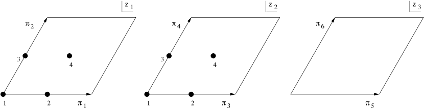
Figure 1: The three two–tori of the $T^{6}/\mathbb{Z}_{6}$ orbifold in the $AAA$–geometry. The fundamental cycles of the $T^{6}$ are denoted by $\pi_{i}$. The fixed points of $\theta^{3}$ on the first two $T^{2}$s, which are relevant for the definition of exceptional cycles, are marked by dots. The third torus is invariant under $\theta^{3}$.

2.2 Three–cycles

To wrap O6-planes and D6-branes on this geometry, we are interested in the number of three–cycles, given by the third Betti number $b_{3}=2(1+h_{2,1})$. According to [28] we have $h_{2,1}=5$, all coming form the orbifold–twisted sector. This leads in total to two bulk cycles inherited from the six–torus and ten exceptional cycles, which wrap a combination of a one–cycle on $T^{3}$ and a two–cycle around one of the $\mathbb{Z}_{3}$ fixed points. General three–cycles will be a combination of bulk and exceptional cycles, but one has to keep in mind that only those combinations are possible in which the bulk cycle passes through the fixed point in question.

2.2.1 Bulk cycles

The factorisable bulk cycles can be defined in terms of a basis of fundamental one–cycles on the three two–tori. For these we use the notation $\pi_{2i-1},\pi_{2i}$ for $T^{2}_{i}$, $i=1,2,3$, as shown in Figure 1. A basis for the bulk cycles can be defined as

$$\rho_{1}=2\left[(1+\theta+\theta^{2})\pi_{1}\otimes\pi_{3}\otimes\pi_{5}\right],$$

$$\rho_{2}=2\left[(1+\theta+\theta^{2})\pi_{2}\otimes\pi_{3}\otimes\pi_{5}\right],$$ (2)

with intersection matrix given by

$$I^{(\rho)}_{ij}=\rho_{i}\circ\rho_{j}=\begin{pmatrix}0&-2\\ 2&0\end{pmatrix}.$$ (3)

Any bulk three–cycle can be expanded using the basis (2.2.1) as

$$\Pi_{a}=Y_{a}\rho_{1}+Z_{a}\rho_{2}.$$ (4)

In terms of the wrapping numbers $n_{i},m_{i}$ of the fundamental one–cycles $\pi_{2i-1}$ and $\pi_{2i}$ the coefficients $Y_{a}$ and $Z_{a}$ read

$$Y_{a} = n_{1,a}n_{2,a}n_{3,a}-m_{1,a}m_{2,a}m_{3,a}-\sum_{i}m_{i,a}m_{j,a}n_{k,a},$$

$$Z_{a} = \sum_{i}m_{i,a}m_{j,a}n_{k,a}+\sum_{i}m_{i,a}n_{j,a}n_{k,a},\quad i,j,k\in\{1,2,3\}\mathrm{cyclic}.$$

From (3) and (4) one computes the intersections between two bulk cycles to be

$$I_{ab}:=\Pi_{a}\circ\Pi_{b}=2(Z_{a}Y_{b}-Y_{a}Z_{b}).$$

The action of the involution (1) on the fundamental one–cycles of the two–tori for the two possible geometries $A$ and $B$ is given by

$$A:\left\{\begin{array}[]{rcl}\pi_{2i-1}&\stackrel{{\scriptstyle\mathcal{R}}}{{\to}}&\pi_{2i-1},\\ \pi_{2i}&\stackrel{{\scriptstyle\mathcal{R}}}{{\to}}&\pi_{2i-1}-\pi_{2i},\end{array}\right.\qquad B:\left\{\begin{array}[]{rcl}\pi_{2i-1}&\stackrel{{\scriptstyle\mathcal{R}}}{{\to}}&\pi_{2i},\\ \pi_{2i}&\stackrel{{\scriptstyle\mathcal{R}}}{{\to}}&\pi_{2i-1}.\end{array}\right.$$

This leads to the following transformations of the bulk cycles (2.2.1) for the six inequivalent geometries,

$$\begin{array}[]{l@{\;\;\rho_1\rmap\;}l@{\quad\rho_2\rmap\;}l}AAA:\hfil\;\;\rho_{1}\stackrel{{\scriptstyle\mathcal{R}}}{{\to}}&\rho_{1},\hfil\quad\rho_{2}\stackrel{{\scriptstyle\mathcal{R}}}{{\to}}&\rho_{1}-\rho_{2},\\ AAB:\hfil\;\;\rho_{1}\stackrel{{\scriptstyle\mathcal{R}}}{{\to}}&\rho_{2},\hfil\quad\rho_{2}\stackrel{{\scriptstyle\mathcal{R}}}{{\to}}&\rho_{1},\\ ABA:\hfil\;\;\rho_{1}\stackrel{{\scriptstyle\mathcal{R}}}{{\to}}&\rho_{2},\hfil\quad\rho_{2}\stackrel{{\scriptstyle\mathcal{R}}}{{\to}}&\rho_{1},\\ ABB:\hfil\;\;\rho_{1}\stackrel{{\scriptstyle\mathcal{R}}}{{\to}}&\rho_{2}-\rho_{1},\hfil\quad\rho_{2}\stackrel{{\scriptstyle\mathcal{R}}}{{\to}}&\rho_{2},\\ BBA:\hfil\;\;\rho_{1}\stackrel{{\scriptstyle\mathcal{R}}}{{\to}}&\rho_{2}-\rho_{1},\hfil\quad\rho_{2}\stackrel{{\scriptstyle\mathcal{R}}}{{\to}}&\rho_{2},\\ BBB:\hfil\;\;\rho_{1}\stackrel{{\scriptstyle\mathcal{R}}}{{\to}}&-\rho_{1},\hfil\quad\rho_{2}\stackrel{{\scriptstyle\mathcal{R}}}{{\to}}&\rho_{2}-\rho_{1}.\end{array}$$ (5)

To obtain the cycles wrapped by O6-planes we have to combine two orbits, invariant under $\Omega\mathcal{R}\theta^{2k}$ and $\Omega\mathcal{R}\theta^{2k+1}$, respectively. For the different geometries we obtain

$$\Pi_{O6}=\left\{\begin{array}[]{lll}AAA:4\rho_{1},&&ABB:6\rho_{2},\\ AAB:4(\rho_{1}+\rho_{2}),&&BBA:4\rho_{2},\\ ABA:2(\rho_{1}+\rho_{2}),&&BBB:4(-\rho_{1}+2\rho_{2}).\end{array}\right.$$ (6)

2.2.2 Exceptional cycles

In addition to the three–cycles inherited from the six–torus we obtain additional, so–called exceptional cycles, which wrap a product of cycles around the $\theta^{3}$–orbifold fixed points (denoted by 1,2,3,4 in Figure 1) and a one–cycle on $T_{3}$. This situation is similar to the one that has been encountered in the case of compactifications on $T^{6}/\mathbb{Z}_{4}$ in [29].

We can choose the following basis of exceptional cycles, invariant under the orbifold projection,

$$\varepsilon_{1} = (e_{21}-e_{41})\otimes\pi_{5}+(e_{41}-e_{31})\otimes\pi_{6},$$

$$\tilde{\varepsilon}_{1} = (e_{31}-e_{41})\otimes\pi_{5}+(e_{21}-e_{31})\otimes\pi_{6},$$

$$\varepsilon_{2} = (e_{12}-e_{14})\otimes\pi_{5}+(e_{14}-e_{13})\otimes\pi_{6},$$

$$\tilde{\varepsilon}_{2} = (e_{13}-e_{14})\otimes\pi_{5}+(e_{12}-e_{13})\otimes\pi_{6},$$

$$\varepsilon_{3} = (e_{22}-e_{44})\otimes\pi_{5}+(e_{44}-e_{33})\otimes\pi_{6},$$

$$\tilde{\varepsilon}_{3} = (e_{33}-e_{44})\otimes\pi_{5}+(e_{22}-e_{33})\otimes\pi_{6},$$

$$\varepsilon_{4} = (e_{23}-e_{42})\otimes\pi_{5}+(e_{42}-e_{34})\otimes\pi_{6},$$

$$\tilde{\varepsilon}_{4} = (e_{34}-e_{42})\otimes\pi_{5}+(e_{23}-e_{34})\otimes\pi_{6},$$

$$\varepsilon_{5} = (e_{24}-e_{43})\otimes\pi_{5}+(e_{43}-e_{32})\otimes\pi_{6},$$

$$\tilde{\varepsilon}_{5} = (e_{32}-e_{43})\otimes\pi_{5}+(e_{24}-e_{32})\otimes\pi_{6},$$ (7)

where we denoted the two–cycles stuck at the fixed points on $T_{1}$ and $T_{2}$ by $e_{ij}$, $i,j=1,\ldots,4$ as shown in Figure 1. The intersection matrix of these exceptional cycles is given by

$$I^{(\varepsilon)}_{ij}:=\bigoplus_{k=1}^{5}\begin{pmatrix}\tilde{\varepsilon}_{k}\circ\tilde{\varepsilon}_{k}&\tilde{\varepsilon}_{k}\circ\varepsilon_{k}\\ \varepsilon_{k}\circ\tilde{\varepsilon}_{k}&\varepsilon_{k}\circ\varepsilon_{k}\end{pmatrix}=\bigoplus_{k=1}^{5}\begin{pmatrix}0&-2\\ 2&0\end{pmatrix}.$$

Under the action (1) of $\mathcal{R}$ the fixed points on the first two $T^{2}$s are mapped into each other as follows,

$$A:\left\{\begin{array}[]{rcl}1&\stackrel{{\scriptstyle\mathcal{R}}}{{\to}}&1,\\ 2&\stackrel{{\scriptstyle\mathcal{R}}}{{\to}}&2,\\ 3&\stackrel{{\scriptstyle\mathcal{R}}}{{\leftrightarrow}}&4\end{array}\right.\qquad B:\left\{\begin{array}[]{rcl}1&\stackrel{{\scriptstyle\mathcal{R}}}{{\to}}&1,\\ 2&\stackrel{{\scriptstyle\mathcal{R}}}{{\leftrightarrow}}&3,\\ 4&\stackrel{{\scriptstyle\mathcal{R}}}{{\to}}&4\end{array}\right.$$

It is possible to combine the bulk cycles (2.2.1) and exceptional cycles (2.2.2), including their images under the orbifold projection, into an unimodular lattice of basic three–cycles [22], which is an important consistency check for completeness of the symplectic basis. Since this particular basis is not very convenient for computations, we will not use it in the following.

3 Model building constraints

In addition to the O6–planes described by (6), we introduce $k$ stacks of D6–branes, wrapping fractional cycles. However, we would like to obtain supersymmetric models which are stable and free of anomalies. Therefore the brane configuration has to fulfil several constraining equations, which we will describe in the following.

3.1 Tadpole cancellation

In order to obtain consistent models we have to make sure that the total charge of the RR seven–forms in the compact space cancels. This imposes a condition on the cohomology classes of these forms, which can be reformulated in homology. Denoting the orientifold image of a cycle $\Pi_{a}$ wrapped by some brane $a$ by $\Pi_{a^{\prime}}$ it reads

$$\sum_{a}N_{a}\left(\Pi_{a}+\Pi_{a^{\prime}}\right)-4\Pi_{O6}=0.$$ (8)

We can split the tadpole condition into two parts containing contributions from the bulk and exceptional cycles, respectively. Since the orientifold planes wrap only bulk cycles according to (6), the contributions from D–branes wrapping exceptional cycles have to cancel among themselves.

Using the basis (4) and the transformation rules (5), we find for the six different geometries the following conditions for $k$ bulk branes with stack sizes $N_{a}$,

$$\begin{array}[]{rlcrl}AAA:&\sum_{a=1}^{k}N_{a}(2Y_{a}+Z_{a})=16,&&ABB:&\sum_{a=1}^{k}N_{a}(Y_{a}+2Z_{a})=24,\\ AAB:&\sum_{a=1}^{k}N_{a}(Y_{a}+Z_{a})=16,&&BBA:&\sum_{a=1}^{k}N_{a}(Y_{a}+2Z_{a})=16,\\ ABA:&\sum_{a=1}^{k}N_{a}(Y_{a}+Z_{a})=8,&&BBB:&\sum_{a=1}^{k}N_{a}Z_{a}=16.\end{array}$$ (9)

3.2 Supersymmetry conditions

In order to preserve $\mathcal{N}=1$ supersymmetry, the bulk cycles have to be calibrated with respect to the same calibration form as the orientifold planes. In our case of three–cycles, this is the holomorphic three–form and this means that the cycles have to be special Lagrangian. Expressed in terms of the expansion coefficients (4) the conditions are given by

$$\begin{array}[]{rlcrl}AAA:&Z_{a}=0,&&ABB:&Y_{a}=0,\\ AAB:&Y_{a}=Z_{a},&&BBA:&Y_{a}=0,\\ ABA:&Y_{a}=Z_{a},&&BBB:&2Y_{a}=-Z_{a}.\end{array}$$ (10)

Since these conditions boil down to the fact that the bulk branes have to wrap the same cycles as the O6–planes, we obtain the result that the intersection number between these branes and the orientifold planes always vanishes,

$$I_{aO6}=\Pi_{a}\circ\Pi_{O6}=0.$$ (11)

To exclude anti–branes from the spectrum, we have to impose one further condition,

$$AAA,AAB,ABA:\;Y_{a}>0,\qquad ABB,BBA,BBB:\;Z_{a}>0.$$ (12)

Fractional branes, being a combination of bulk and exceptional cycles, preserve half of the supersymmetry, if the bulk part obeys (11) and (12), and the exceptional part comes from fixed points that are traversed by the bulk cycle. In total there are 128 different possible combinations of exceptional cycles for a given bulk cycle. All possible combinations can be found in Tables 23 and 24 of [22].

3.3 K–theory constraints

In addition to the constraints from tadpole cancellation and supersymmetry, we have to demand that the four–dimensional models are anomaly–free. Cancellation of local gauge anomalies is guaranteed by a generalised Green–Schwarz mechanism, yet there exists the possibility to obtain a global gauge anomaly [30], which can be deduced from a K–theory analysis. In the case of our models, this condition requires an even amount of chiral matter from $Sp(2)$ probe branes, inserted in the geometric setup [31]. $Sp(2)$ gauge groups are carried by branes that are invariant under the orientifold action. Unfortunately this is not the only possible gauge group for these branes, they can equally well support an $SO(2)$ group. To differentiate between these two, one has to go beyond the algebraic approach that suffices to calculate the tadpole, the susy constraints and the chiral matter content. It is necessary to analyse the open string Möbius amplitude for each possible brane.

Fortunately the geometrical setup of the $\mathbb{Z}_{6}$ orientifold is such that we do not have to worry about this issue. In fact, it can be generally proved that all possible solutions that fulfil the tadpole and susy constraints will automatically satisfy the stronger condition where all possible orientifold–invariant probe branes are used. In this case we obtain the following condition for a model with $k$ stacks of branes,

$$\sum_{a=1}^{k}N_{a}\Pi_{a}\circ\Pi_{p}\equiv 0\mod 2,$$ (13)

and this equation should hold for any probe brane $p$ invariant under the orientifold map.

Because of this property and the fact that the bulk part of the probe branes does not intersect with the bulk part of all other branes, several of the terms in (13) vanish and we can rewrite it as

$$\sum_{i=1}^{5}\left(\sum_{a=1}^{k}N_{a}s_{a}^{i}\right)r_{p}^{i}\equiv 0\mod 2,$$ (14)

where the values $s_{a}^{i}$ are the coefficients of the cycles of brane $a$ which are odd under the orientifold projection and the $r_{p}^{i}$ parametrise the cycles of the probe branes which are even under the orientifold map. Note that we are summing over exactly half of the dimension of the basis of exceptional three–cycles. However, not all of the $r_{p}^{i}$ are independent, since the probe branes are bound to be on top of the orientifold planes. An explicit calculation shows that there exist only eight different possibilities and that the coefficients $r_{p}^{i}$ are always even. Therefore (14) is always fulfilled.

3.4 Open string spectrum

The massless chiral states arising at the intersection of different stacks of D–branes and at the intersection of branes with their orientifold mirrors and the orientifold planes, can be computed from the intersection numbers. In general a stack of $N$ branes supports a $U(N)$ gauge group, unless the three–cycle wrapped by this stack lies on top of the orientifold plane. In this case we are dealing with an $SO(N)$ or $Sp(N)$ group.

To compute the non–chiral spectrum, one has to analyse the open string amplitudes. In our statistical analysis we will not do so, but concentrate on the chiral spectrum only. As shown in Table 1, we obtain chiral matter in a bi–fundamental representation at the intersection of two stacks $a$ and $b$ with $N_{a}$ and $N_{b}$ branes, respectively. In addition there is the possibility for each stack to contribute matter in the symmetric and antisymmetric representations of the gauge group. From the discussion in Section 3.2 it follows that the amount of symmetric and antisymmetric representations will always be the same, since there can be no contribution from the intersection with the orientifold planes. Moreover, it is crucial to work with fractional cycles, since all bulk cycles that occur lie on top of the orientifold plane and do hence not intersect which each other.

representations	multiplicity
$(\mathbf{N}_{a},\overline{\mathbf{N}}_{b})$	$\Pi_{a}\circ\Pi_{b}$
$(\mathbf{N}_{a},\mathbf{N}_{b})$	$\Pi_{a}\circ\Pi^{\prime}_{b}$
$\mathbf{Sym}_{a}$	$\frac{1}{2}\left(\Pi_{a}\circ\Pi_{a^{\prime}}-\Pi_{a}\circ\Pi_{O6}\right)$
$\mathbf{Anti}_{a}$	$\frac{1}{2}\left(\Pi_{a}\circ\Pi_{a^{\prime}}+\Pi_{a}\circ\Pi_{O6}\right)$

Table 1: Multiplicities of the chiral spectrum.

3.5 Embedding of the standard model

Since our final goal is to quantify the number of standard model–like vacua that can be found in this type of compactifications, we have to chose a way to realise the gauge group and chiral matter content of the MSSM in terms of intersecting branes. In the present work we will consider only one type of embedding, mainly for two reasons. One is given by external constraints on computational power and feasibility. The second one lies in the special properties of the orbifold we are investigating. Since we saw in the previous section that the amount of symmetric and antisymmetric representations is always equal, several possible constructions of standard model spectra that use antisymmetric representations of $SU(2)$ cannot be realised, unless one also allows for chiral matter in the symmetric representation, which is not desirable from a phenomenological point of view.

particle	representation	multiplicity
$Q_{L}$	$(\mathbf{3},\overline{\mathbf{2}})_{0,0}+(\mathbf{3},\mathbf{2})_{0,0}$	$I_{ab}+I_{ab^{\prime}}$
$U_{R}$	$(\overline{\mathbf{3}},\mathbf{1})_{-1,0}+(\overline{\mathbf{3}},\mathbf{1})_{0,-1}$	$I_{a^{\prime}c}+I_{a^{\prime}d}$
$D_{R}$	$(\overline{\mathbf{3}},\mathbf{1})_{1,0}+(\overline{\mathbf{3}},\mathbf{1})_{0,1}$	$I_{a^{\prime}c^{\prime}}+I_{a^{\prime}d^{\prime}}$
$L$	$(\mathbf{1},\overline{\mathbf{2}})_{-1,0}+(1,\overline{\mathbf{2}})_{0,-1}+(\mathbf{1},\mathbf{2})_{-1,0}+(\mathbf{1},\mathbf{2})_{0,-1}$	$I_{bc}+I_{bd}+I_{b^{\prime}c}+I_{b^{\prime}d}$
$E_{R}$	$(\mathbf{1},\mathbf{1})_{1,1}$	$I_{cd}$
$N_{R}$	$(\mathbf{1},\mathbf{1})_{1,-1}$	$I_{cd^{\prime}}$

Table 2: Realisation of standard model particles with four stacks of branes. The notation in the second column gives the representation under $SU(3)$ and $SU(2)$ in brackets with the charges under the $U(1)$s of the third and fourth stack as subscripts.

The construction we will use in Section 6.5 for the analysis of the frequency distribution of standard models is well–known and has been used in many model building approaches of intersecting branes. It consists of two stacks of branes ($a$ and $b$) with gauge groups $U(3)$ and $U(2)$, and two branes ($c$ and $d$) with a $U(1)$ group. The standard model spectrum is realised through chiral matter transforming in bifundamental representations of the gauge groups. The complete spectrum and the assignment to particles is given in Table 2.

The hypercharge $Q_{Y}$ is realised in this construction as a combination of the $U(1)$ charges $Q_{i}$, with $i=\{a,b,c,d\}$ of the four branes. Explicitly it is given by

$$Q_{Y}=\frac{1}{6}Q_{a}+\frac{1}{2}Q_{b}+\frac{1}{2}Q_{c}.$$

4 Finiteness of solutions

An important question that we would like to answer before analysing the four–dimensional models in detail concerns the finiteness of possible solutions to the constraining equations outlined in Section 3. To answer this question, it is sufficient to analyse the solution space of the system of equations (9) and (10). We do not have to take the analogue expressions for the exceptional cycles into account, although the set of solutions is greatly enhanced by models containing exceptional cycles, because the number of possible combinations of these cycles is always finite (cf. Section 3.2). The K–theory constraints will play no rôle anyway, as has been argued above.

One important drawback of our approach has to be mentioned here. We cannot make any statement about the dependence of the number of solutions on the complex structure moduli. The complex structures of the three two–tori are fixed by the requirement to be compatible with the orbifold projection. Since $h_{2,1}=5$, we find ten complex structure moduli in the twisted sector. We do not analyse the blow up of the orbifold singularities and can therefore not make any statements about the behaviour of our models away from the orbifold point. Having said this, we will continue to prove that there is only a finite number of models at this point in moduli space.

After the susy conditions are fulfilled, we are left with one tadpole condition for each possible geometry, according to (9). It will contain one unknown wrapping number ($Y$ or $Z$, depending on the geometry), which is always positive according to (12). Therefore it follows trivially that the remaining unknown in the tadpole equations is bounded from above by the orientifold charge, which also depends on the geometry, but will never be greater than 24. To proof the finiteness of the number of models, it remains to be shown that the possible combinations of wrapping numbers $\{n_{i},m_{i}\}$, which make up $Y$ and $Z$ according to (2.2.1), are always finite.

In the following we will give an explicit proof for the $AAA$–geometry, the other five possibilities can be treated analogously. In order to simplify the discussion and reflect the symmetries of the problem, we define new variables for the wrapping numbers on the first two tori, while keeping the wrapping numbers on the third torus explicit.

$$\alpha := m_{1}m_{2}+n_{1}m_{2}+n_{2}m_{1},$$

$$\qquad\beta := n_{1}n_{2}+n_{1}m_{2}+n_{2}m_{1}.$$ (15)

Exchanging the first two tori, which is a symmetry of the geometric setup, will leave $\alpha$ and $\beta$ invariant. In terms of $\alpha,\beta,n_{3},m_{3}$ (10) reads

$$Z=n_{3}\alpha+m_{3}\beta=0.$$ (16)

Since we know from (12) that $Y$ has to be positive, one stack of branes has to contribute a finite value $0<T<16$ to the tadpole constraint. This amounts to a second equation,

$$Y=n_{3}(\beta-\alpha)-m_{3}\alpha=T.$$ (17)

To analyse the possibility of an infinite set of solutions to (16) and (17), we have to distinguish between the cases $n_{3}=0$ and $n_{3}\neq 0$.

$\mathbf{n_{3}=0}$:

Since $n_{3}$ and $m_{3}$ cannot vanish simultaneously, we get from (16) that

$$\beta=n_{1}(n_{2}+m_{2})+n_{2}m_{1}=0.$$ (18)

and from (17) we obtain

$$-m_{3}\alpha=-m_{3}\left(m_{2}(m_{1}+n_{1})+n_{2}m_{1}\right)=T.$$ (19)

An infinite number of solutions can only exist, if there is an infinite series of solutions to $\beta=0$ or $\alpha=\mathrm{const}$. Both cases can be treated analogously, so let us pick one of them and examine $\beta=0$. Again we analyse two cases, depending on the value of $n_{1}$. If $n_{1}=0$, we get from (18) that $n_{2}=0$ and (19) reads $-m_{1}m_{2}m_{3}=T$, which puts bounds on $\{m_{i}\}$. If $n_{1}\neq 0$, we can rewrite (18) as

$$m_{2}=-\frac{n_{2}}{n_{1}}\left(n_{1}+m_{1}\right).$$

Substituting this into (19) leads to

$$\frac{m_{3}n_{2}}{n_{1}}\left(n_{1}^{2}+m_{1}^{2}+n_{1}m_{1}\right)=T.$$

To obtain an infinite series, the expression in brackets would have to have an infinite number of solutions. This is not possible, since the term always defines an ellipse, which supports only a finite number of integer–valued points.

$\mathbf{n_{3}\neq 0}$:

In this case we can rewrite (16) as

$$\alpha=-\frac{m_{3}}{n_{3}}\beta.$$ (20)

Substitution in (17) leads to

$$\left(n_{3}+m_{3}+\frac{m_{3}^{2}}{n_{3}}\right)\beta=T.$$ (21)

The expression in brackets defines again an ellipse and can have only a finite number of solutions. The remaining possibility would be that there exists an infinite series to $\beta=n_{1}n_{2}+n_{1}m_{2}+n_{2}m_{1}=\mathrm{const}$.

Let us analyse the different possibilities for $\{n_{1},m_{1},n_{2},m_{2}\}$. If $n_{1}$ or $n_{2}$ are zero, we can see immediately that an infinite series is impossible. If $m_{1}$ vanishes instead, we obtain $n_{1}(n_{2}+m_{2})=\mathrm{const}$. If there should exist an infinite series, $n_{2}$ and $m_{2}$ have to be unbounded. Using the definition (4) we deduce that $\alpha=n_{1}m_{2}$ has would be unbounded as well. This is only consistent with (20) if $m_{3}$ would grow beyond all bounds, which is in contradiction to (21). The argument can be repeated analogously for $m_{2}$ vanishing.

So we are left with the case of $n_{1},n_{2},m_{1},m_{2}$ all non–vanishing. In this situation we can rewrite $\beta$ as

$$n_{1}n_{2}\left(1+\frac{m_{2}}{n_{2}}+\frac{m_{1}}{n_{1}}\right)=\mathrm{const},$$

which can have only an infinite number of solutions, if $m_{2}n_{1}=-m_{1}n_{2}$ with $m_{1},m_{2}$ unbounded. But in this case we find $\alpha$ to be unbounded, which is not possible with $\beta$ bounded at the same time. This completes the proof that there can only be a finite number of solutions to the tadpole and supersymmetry conditions.

5 Methods of analysis

In the following we describe the computational methods we used to obtain an ensemble of solutions to the tadpole, supersymmetry and K–theory conditions. The results of the statistical analysis are based on this explicitly calculated ensemble.

5.1 Choice of basis

It turns out that it is convenient to use a different basis of three–cycles for the computational analysis, because it makes the tadpole conditions (8) for the bulk cycles and exceptional cycles more uniform. The basis consists of $\mathcal{R}$ even cycles $\eta_{i}$ and $\mathcal{R}$ odd cycles $\lambda_{i}$, $i=0,\ldots,5$, which are given in terms of the basis of bulk cycles (2.2.1) and exceptional cycles (2.2.2) for the different geometries as

$$\vec{\eta} = \frac{1}{2}\left\{\begin{array}[]{rl}AAA:&(\rho_{1},-\varepsilon_{1}+2\tilde{\varepsilon}_{1},-\varepsilon_{2}+2\tilde{\varepsilon}_{2},-\varepsilon_{3}+2\tilde{\varepsilon}_{3},\tilde{\varepsilon}_{4}-\varepsilon_{5}+\tilde{\varepsilon}_{5},\varepsilon_{4}-\varepsilon_{5}),\\ AAB:&(\rho_{1}+\rho_{2},-\varepsilon_{1}+\tilde{\varepsilon}_{1},-\varepsilon_{2}+\tilde{\varepsilon}_{2},-\varepsilon_{3}+\tilde{\varepsilon}_{3},\varepsilon_{4}-\tilde{\varepsilon}_{5},-\tilde{\varepsilon}_{4}+\varepsilon_{5}),\\ ABA:&(\rho_{1}+\rho_{2},-\varepsilon_{1}+2\tilde{\varepsilon}_{1},2\varepsilon_{2}-\tilde{\varepsilon}_{2},-\varepsilon_{5}+2\tilde{\varepsilon}_{5},\tilde{\varepsilon}_{3}-\varepsilon_{4}+\tilde{\varepsilon}+4,\varepsilon_{3}-\varepsilon_{4}),\\ ABB:&(\rho_{2},-\varepsilon_{1}+\tilde{\varepsilon}_{1},\varepsilon_{2},-\varepsilon_{5}+\tilde{\varepsilon}_{5},\varepsilon_{3}-\tilde{\varepsilon}_{4},-\tilde{\varepsilon}_{3}+\varepsilon_{4}),\\ BBA:&(\rho_{2},2\varepsilon_{1}-\tilde{\varepsilon}_{1},2\varepsilon_{2}-\tilde{\varepsilon}_{2},2\varepsilon_{3}-\tilde{\varepsilon}_{3},\tilde{\varepsilon}_{4}-\tilde{\varepsilon}_{5},\varepsilon_{4}-\tilde{\varepsilon}_{4}+\varepsilon_{5}),\\ BBB:&(-\rho_{1}+2\rho_{2},\varepsilon_{1},\varepsilon_{2},\varepsilon_{3},-\varepsilon_{4}+\tilde{\varepsilon}_{4}-\tilde{\varepsilon}_{5},\varepsilon_{4}+\varepsilon_{5}),\end{array}\right.$$ (28)

and

$$\vec{\lambda} = \frac{1}{2}\left\{\begin{array}[]{rl}AAA:&(-\rho_{1}+2\rho_{2},\varepsilon_{1},\varepsilon_{2},\varepsilon_{3},\varepsilon_{4}+\varepsilon_{5},-\tilde{\varepsilon}_{4}-\varepsilon_{5}+\tilde{\varepsilon}_{5}),\\ AAB:&(-\rho_{1}+\rho_{2},\varepsilon_{1}+\tilde{\varepsilon}_{1},\varepsilon_{2}+\tilde{\varepsilon}_{2},\varepsilon_{3}+\tilde{\varepsilon}_{3},-\tilde{\varepsilon}_{4}-\varepsilon_{5},-\varepsilon_{4}-\tilde{\varepsilon}_{5}),\\ ABA:&(-\rho_{1}+\rho_{2},\varepsilon_{1},-\tilde{\varepsilon}_{2},\varepsilon_{5},\varepsilon_{3}+\varepsilon_{4},-\tilde{\varepsilon}_{3}-\varepsilon_{4}+\tilde{\varepsilon}_{4}),\\ ABB:&(-2\rho_{1}+\rho_{2},\varepsilon_{1}+\tilde{\varepsilon}_{1},\varepsilon_{2}-2\tilde{\varepsilon}_{2},\varepsilon_{5}+\tilde{\varepsilon}_{5},-\tilde{\varepsilon}_{3}+\varepsilon_{4},-\varepsilon_{3}-\tilde{\varepsilon}_{4}),\\ BBA:&(-2\rho_{1}+\rho_{2},-\tilde{\varepsilon}_{1},-\tilde{\varepsilon}_{2},-\tilde{\varepsilon}_{3},\varepsilon_{4}-\varepsilon_{5}+\tilde{\varepsilon}_{5},-\tilde{\varepsilon}_{4}-\tilde{\varepsilon}_{5}),\\ BBB:&(-\rho_{1},\varepsilon_{1}-2\tilde{\varepsilon}_{1},\varepsilon_{2}-2\tilde{\varepsilon}_{2},\varepsilon_{3}-2\tilde{\varepsilon}_{3},\varepsilon_{4}-\varepsilon_{5},-\tilde{\varepsilon}_{4}+\varepsilon_{5}-\tilde{\varepsilon}_{5}).\end{array}\right.$$ (35)

The expansion of a three–cycle in terms of this basis reads

$$\Pi_{a}=\vec{r}\cdot\vec{\eta}+\vec{s}\cdot\vec{\lambda}=\sum_{i=0}^{5}\left(r_{a}^{i}\eta_{i}+s_{a}^{i}\lambda_{i}\right),$$

with expansion coefficients $r^{i},s^{i}$, $i=0\ldots 5$. The tadpole equations are given by

$$\sum_{a}N_{a}\vec{r}_{a}=4\vec{r}_{O6},$$ (36)

The zeroth entry of $\vec{r}_{O6}$ can be read off from (9), while all others have to vanish, since the orientifold planes do not contribute to the tadpole equations of the exceptional cycles.

In terms of this new basis the intersection between two stacks of branes $a$ and $b$ defined by cycles $\Pi_{a}$ and $\Pi_{b}$ reads

$$I_{ab}=\Pi_{a}\circ\Pi_{b}=\frac{1}{2}\left(\vec{s}_{a}\cdot\vec{r}_{b}-\vec{r}_{a}\cdot\vec{s}_{b}\right).$$ (37)

5.2 Algorithm

To obtain a large number of models that fulfil the constraining equations, we used several computers to generate the solutions, which were subsequently stored in a database for later analysis. A priori no constraints have been imposed on the models besides being consistent solutions to the tadpole and supersymmetry conditions.

As mentioned before, the model building constraints described in Section 3 can be treated separately for bulk and exceptional cycles. The first part of the computer program we use, which searches for pure bulk configurations, employs the partition algorithm used in [11] to find all possible realisations of the left hand side of equation (36). Subsequently it runs through a certain range of pairwise coprime wrapping numbers searching for groups $(n_{i},m_{i}),\medspace i=1,2,3$ that yield the desired $r^{0}$ values. Care has to be taken to avoid multiple counting of cycles which are identified under the orbifold or orientifold action. Explicitly, two of the wrapping numbers are restricted to be always $>0$ and the wrapping numbers on the third torus, $(n_{3},m_{3})$ have been chosen to be both odd. In this way no double counting of solutions which are related by a geometric symmetry of the problem will occur. Subsequently the program checks the bulk supersymmetry conditions (10) and (12), which amount to $r_{a}>0,\medspace s_{a}^{0}=0$ in the notation introduced above. Finally one finds configurations of bulk cycles, which fulfil all consistency conditions, by combining the results of the previous steps.

According to tables 23 and 24 in [22] $128$ exceptional cycles, which already satisfy the supersymmetry conditions, arise for one single bulk cycle. The second part of our program runs through all $128^{k}$ possible combinations of exceptional cycles for a bulk configuration with $k$ stacks and checks the exceptional tadpole conditions explicitly. Unfortunately there is no way to exclude part of these $128^{k}$ combinations a priori and we have no choice but to compute every single one of them in order to perform a complete analysis. As a consequence the time necessary for the computation scales exponentially with the number of stacks and could reach the realm of years or even decades. In the following we will thus only present full statistics for models with a low number of stacks. For configurations with a higher number of stacks we randomly select a fraction of the $128^{k}$ possible combinations. As we will argue in the next section, these randomly chosen subsets can be trusted to resemble the full statistical distributions and are therefore sufficient to make statements about frequency distributions of gauge group properties and chiral matter content.

6 Results

In the following we present the results of a statistical analysis of the ensemble of solutions to the tadpole, supersymmetry and K–theory constraints, which have been computed as outlined in the last section.

As already mentioned before, a full analysis of all possible models is as yet impossible. This comes from the simple fact that the total number of solutions is of the order $10^{28}$, as we are going to show in the following, and an explicit computation of every single solution is beyond reach of contemporary computer technology. Therefore we used the technique of choosing random subsets of possible solutions which in turn were analysed in detail. As it turns out this method is perfectly sufficient for a statistical analysis.

After a more detailed explanation of this random method, we discuss the total number of solutions. Then we turn to discuss frequency distributions of various properties of the models, in particular the gauge group factors, the total rank and the chiral matter content. Finally we look for solutions that realise the gauge group of the standard model, discuss their suppression within the set of all solutions and the properties of the hidden sector gauge group.

Along the way we compare the results with an analysis of $\mathbb{Z}_{2}\!\times\!\mathbb{Z}_{2}$ models. We only cite the relevant results here, a summary of the statistical analysis that has been done in that case can be found in [14].

6.1 Choosing random subsets

The most time–consuming part of computing full solutions is given by adding exceptional cycles to configurations of bulk cycles that already fulfil the tadpole condition. As explained in Section 5.2, the bulk solutions are obtained using a fast partition algorithm, while for the exceptional part there is no other way then to run through all $128^{k}$ possible combinations and check if they fulfil the constrains. This algorithm clearly scales exponential with the number of stacks $k$, such that a complete survey of models with more then three stacks is not feasible.

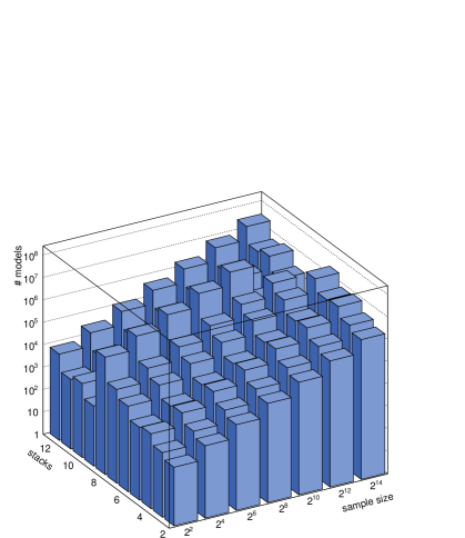
Figure 2: The number of solutions for different numbers of stacks and sizes of the random sample.

Nevertheless, as we will explain shortly, we are able to derive quite robust statistical statements about the full set of solutions. To do so, we apply a procedure to obtain random subsets of the $128^{k}$ possible ways to add exceptional cycles to a bulk solution. If the total number of solutions is large enough, it is possible to assume a linear dependence between the size of the sample $s$ and the number of solutions $n(s)$. Moreover, the gradient can be used to compute the total number of solutions $n_{tot}(k)$ for a given stack size, if we assume that this number scales with $128^{k}$.

To summarise, we assume that the following equation holds approximately,

$$n_{tot}\approx\frac{n(s)}{s}128^{k}.$$ (38)

In Figure 2 the number of solutions for different numbers of stacks and sizes of random samples is shown. Although not clearly visible in this three dimensional plot, the number of solutions grows indeed linearly with the size of the random sample. The accuracy of the linear fit increases with the number of stacks. According to (38), the slope of the logarithmic plot gives the average number of full solutions per bulk configuration, which varies between $10^{2}$ for the two–stack models and $4.3\times 10^{4}$ in the case of models with eight stacks.

stacks	exact	estimate	error
$2$	$1.7068\times 10^{6}$	$1.7079\times 10^{6}$	$<7\times 10^{-4}$
$3$	$3.9816\times 10^{8}$	$3.9818\times 10^{8}$	$<6\times 10^{-5}$

Table 3: Exact number of solutions and estimated values for models with two and three stacks of branes and the relative error of the estimate.

Using the exact results in the two– and three–stack case we can compare the total number of solutions with the estimated result from the random procedure. The results of this comparison are shown in Table 3. It turns out that the estimate is correct up to an error smaller then 0.7‰ in the case of models with two stacks and even an order of magnitude less in the case of three stacks. Although we cannot completely rule out that something dramatically different happens for models with a larger number of stacks, this seems very unlikely. Our results rather suggest that on the contrary one might conjecture that the estimate gets better for larger stack size $k$. This can be justified given that the deviation from linearity in the scaling gets smaller for larger $k$.

It can therefore be expected that the results obtained using the random method are sufficient for a statistical analysis and that we are allowed to extrapolate the frequency distributions obtained for a random sample to the full set of solutions using the relation (38). However, it should be emphasised that a good approximation of the number of solutions is not enough to obtain an accurate description of the properties of the models. Therefore we always perform a check for each distribution against the models with two and three stacks to see if the frequency distributions of the complete solution and the extrapolated distributions from the random samples do agree. In particular for properties of the gauge group we expect the method to work very well, since the gauge group factors depend on the bulk configuration only.

6.2 Total number of solutions

In order to make statistical statements about the probability of certain properties of solutions, it is certainly important to know about how many solutions we are talking. In Figure 3 the number of solutions depending on the number of stacks is given. The left figure shows the number of solutions to the bulk equations alone, not including exceptional cycles, while the right figure contains the full result of consistent models. The minimum number of stacks is two in both cases, while the maximum is twelve, which can be deduced immediately from the tadpole equations (36). Remember that all variables are positive and the maximum value of the right hand side is $24$, while the wrapping number on the left hand side is always a multiple of two.

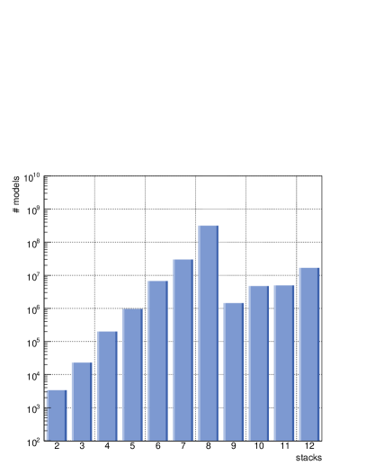
(a)

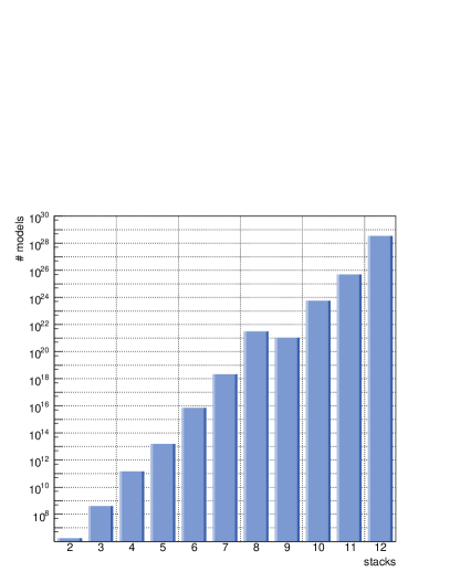
(b)

Figure 3: Logarithmic plot of the total number of solutions to the tadpole equations. The left plot (a) shows only bulk solutions, while the right one (b) show the full set of solutions, including exceptional cycles.

Let us begin with an analysis of supersymmetric solutions to the bulk part of the tadpole conditions (9) alone. Note that these configurations are just an intermediate step to a full solution, since we need to include exceptional cycles to obtain consistent models. Nevertheless it is an interesting question to ask how many solutions of the bulk equations exist, since this gives an overview of the number of candidate solutions to the full tadpole and susy constraints. As explained above, we will have to consider $128^{k}$ possibilities of configurations of exceptional cycles for each bulk solution.

As one can deduce from Figure 3(a), the maximum number of solutions of possible bulk cycles is obtained for models with $8$ stacks. In principle one would assume that the number of possible configurations grows dramatically with the number of stacks, since naively the number of models with $k$ stacks should be proportional to the number of factorisations of integer partitions of length $k$. However, the negative contribution of the orientifold planes to the tadpole equation is different for the six possible geometries. For the $AAA$, $AAB$, $BBA$ and $BBB$ cases we get a total contribution of $16$, while in the $AAB$ and $ABB$ cases we obtain $8$ and $24$, respectively. Keeping in mind that there is a factor of two on the left hand side of $\eqref{eqtadbulk}$ and that all brane contributions are positive, one finds that the condition for models with $AAB$ geometry can only be fulfilled if the number of stacks is smaller then five. In the case of $AAA$, $AAB$, $BBA$ and $BBB$ models with a maximum of eight stacks are possible. This explains the relatively small contributions for models with more then eight stacks.

After completing the models with exceptional cycles, the picture changes quite a bit. This is due to the aforementioned fact that there are in principle $128^{k}$ possible configurations of exceptional cycles for each bulk configuration. Not all of them are consistent, in the sense that they fulfil the full tadpole equations (36), but as we have shown in Section 6.1 the total number of solutions scales precisely with this number, multiplied by a coefficient of order $10^{2}$ to $10^{4}$. This explains the domination of models with twelve stacks, that can be seen in Figure 3(b). As we will see in the following, this dominance of models with large stack numbers has a large impact on the statistical distributions.

Using the randomly generated solutions for all possible numbers of stacks we can compute the total number of models to be $3.43\times 10^{28}\pm 1\%$. Since the linearity of the growth of solutions increases with large numbers of stacks, we can estimate the error in this calculation to be smaller then the relative error calculated explicitly for the two stack models in the last section.

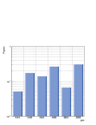
(a)

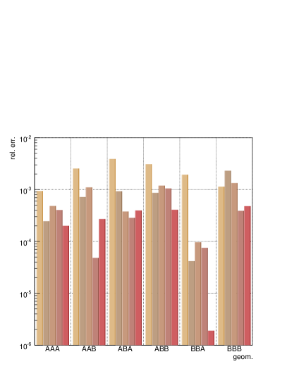
(b)

Figure 4: Relative contributions of the different geometries to the full set of solutions for models with three stacks. The right figure (b) shows the relative error between the random solutions for different stack sizes and the full set of solutions. The stacks sizes are 4, 16, 64, 256, 1024, 4096 and 16384 (from left to right).

To complete the picture, we analyse the individual contributions of the different geometries. This will also serve as a test of the random method that we used to obtain the statistical distributions. As can be seen in Figure 4(a), the largest contribution comes from the $BBB$ geometry. Concerning the relative error we make using the random method, it is found to be sufficiently small. As shown in Figure 4(b), already at a random sample size of $64$ out of $2^{21}$ combinations of exceptional cycles, we obtain an error smaller then 1%.

6.3 Gauge groups

We consider two properties of the gauge group of the models, which consists of a product of $U(N)$, $SO(2N)$ and $Sp(2N)$ groups. Firstly we analyse the distribution of the total rank, defined as

$$r:=\sum_{a=1}^{k}N_{a}.$$ (39)

In a second step we discuss the probability to find one brane with a gauge group of rank $N$. Both properties are obviously important to classify models which resemble the standard model.

6.3.1 Rank distribution

The frequency distribution of the total rank, see Figure 5(a), grows exponentially and reaches a maximum at rank $12$. This behaviour can be explained by the dominance of models with twelve stacks of branes. The exponential scaling of the total rank is directly related to the exponential scaling of the total number of solutions, because these are dominated by models with an $U(1)$ gauge group. This follows from the solutions to the tadpole equations, which are given as factorisations of partitions of the orientifold charge. The factor one is not only the number with the highest abundance in integer partitions, but it is in fact the only possible gauge group in models with twelve stacks of branes, as follows directly from the positivity of all variables in the tadpole equation.

This rank distribution has to be considered with some caution however, since it includes all possible $U(1)$ factors of the spectrum. It is well known that some of the $U(1)$s will acquire a mass in the effective theory. This could happen through a generalised Green–Schwarz mechanism that compensates a mixed gauge anomaly involving the $U(1)$ in question, but more general cases are possible. It would be of course very interesting to study the rank distribution that one obtains after subtracting the massive $U(1)$ factors, but for the full set of models the necessary computations are not feasible. In the analysis of models that contain the gauge group of the standard model in Section 6.5, we will make sure that at least one massless $U(1)_{Y}$ (the hypercharge) exists, but a quantitative statement about the number of massive $U(1)$s in the general case is beyond the means of our approach.

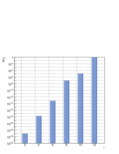
(a)

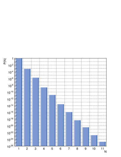
(b)

Figure 5: Frequency distributions of (a) the total rank $r$ and (b) the probability to find a gauge group of rank $N$.

One striking fact of the rank distribution still has to be explained: There are only solutions with even rank. This is a consequence of the specific $\mathbb{Z}_{6}$ geometry and different from other orbifold models, as for example the $\mathbb{Z}_{2}\!\times\!\mathbb{Z}_{2}$ models we already mentioned. To show why this is always the case, we have to take a closer look at the tadpole equation (36). The right hand side is always a multiple of $4$, depending on the geometry. Therefore we have to have

$$\sum_{a\in A}S_{a}\equiv 0\mod 4,\qquad\mbox{with}\quad S_{a}:=N_{a}Y_{a},\quad A:=\{1,\ldots,k\}.$$ (40)

We split the sum over $S_{a}$ into two parts, consisting of only even and only odd values:

$$\sum_{a\in A}S_{a}=\sum_{a\in O}S_{a}^{(odd)}+\sum_{a\in E}S_{a}^{(even)},\qquad\mbox{with}\quad O\cup E=A,\quad O\cap E=\emptyset.$$

The equivalence (40) can only be fulfilled, if there is an even number of $S_{a}^{odd}$. Writing the total rank (39) as

$$r=\sum_{a\in A}N_{a}=\sum_{a\in O}N_{a}+\sum_{a\in E}N_{a},$$ (41)

we get that the first part of this sum is even. Here we used that all branes in the set $O$ have to obey $N_{a}\equiv 1\mod 2$, for $S_{a}^{(odd)}\equiv 1\mod 2$. For the second part of (41) to be even, it is enough to show that $Y_{a}$ is always odd. This can be done by writing the wrapping number in terms of the fundamental torus wrapping numbers, similar to what we did in Section 4. From

$$Y=n_{2}(\alpha-\beta)-m_{2}(\beta)\quad,\quad Z=n_{2}\beta+m_{2}\alpha=0$$ (42)

and the constraints $(n_{2},m_{2})\equiv(1,1)\mod 2$, explained in Section 5, we obtain from the second equation in (42) that $\alpha\equiv\beta\mod 2$ and therefore $Y\equiv 1\mod 2$. This completes the proof.

6.3.2 Gauge group factors

In Figure 5(b) the probability to find a gauge group of rank $N$ is shown. For the reason explained in the last paragraph, namely the abundance of $U(1)$ gauge factors, the probability to find one brane with gauge group of rank one is almost 100%. The distribution falls off exponentially for larger $N$, which is again due to the exponential scaling of the number of solutions with the number of stacks.

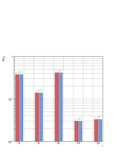
(a)

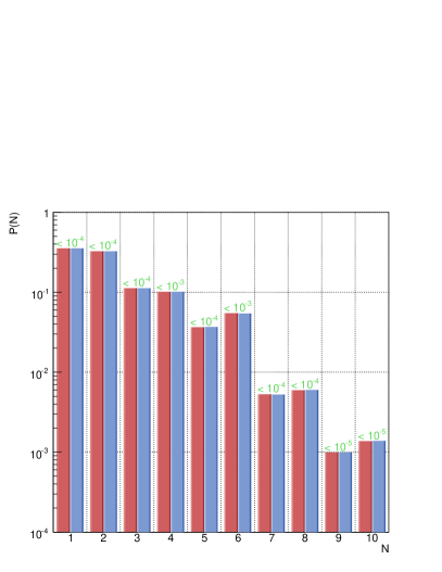
(b)

Figure 6: Comparison of the results for the distribution of (a) the total rank $r$ and (b) the probability to find a rank $N$ gauge factor for models with three stacks of branes. The full result is given by the red bars on the left, while the solutions obtained using a random set of $2^{14}$ exceptional cycles are shown as blue bars on the right. An upper bound on the relative error is given by the value above each bar.

As in the case of the total number of solutions, we have obtained the distributions using an extrapolation of results from random subsets. To check the validity of this approach, we compare with the full set of models in the case of three stacks of branes. The result is shown in Figure 6. For both cases, the total rank distribution as well as the probability distribution of single gauge factors, we obtain very accurate results. The relative error is always smaller then 1‰in both cases.

6.4 Mean chirality

To understand on a qualitative level how many of the solutions are chiral, we analyse the “mean chirality” of the set of solutions. To do so, we define the mean chirality to be the average of chiral representations in each model. This definition is identical to the one used in the statistical analysis of $\mathbb{Z}_{2}\!\times\!\mathbb{Z}_{2}$ orbifold models (cf. Section 3.2.2 of [14]). For a model with $k$ stacks we define the mean chirality $\chi$ as

$$\chi:=\frac{2}{k(k+1)}\sum_{\begin{subarray}{c}a,b=0\\ a<b\end{subarray}}^{k}\left|I_{a^{\prime}b}-I_{ab}\right|=\frac{2}{k(k+1)}\sum_{\begin{subarray}{c}a,b=0\\ a<b\end{subarray}}^{k}\left|\vec{s}_{a}\cdot\vec{r}_{b}\right|,$$ (43)

where we used the definition of the intersection $I_{ab}$ in terms of the $\eta,\lambda$–basis (37).

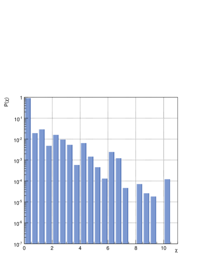
(a)

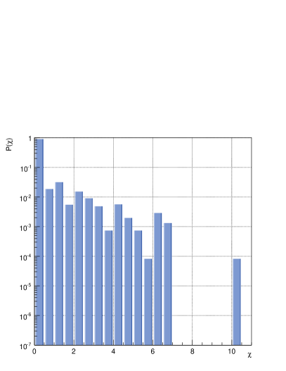
(b)

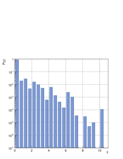
(c)

(d)

Figure 7: Frequency distribution of the mean chirality $\chi$ for models with three stacks of branes. Shown are the full set of solutions (a) and three sets generated using randomly chosen subsets of 64 (b), 1024 (c) and 16384 (d) out of all 2097152 possible combinations of exceptional cycles.

Before considering all random subsets, we have to make sure that the method can also be trusted in this case, since we are asking a different question then in the case of gauge factors or rank distributions. The definition of the mean chirality (43) involves a summation over intersection numbers. These depend very much on the choice of exceptional cycles, in contrast to the properties of the gauge group, which depend only on the configuration of bulk cycles.

In Figure 7 we compare the distribution obtained from the full set of solutions for models with three stacks of branes, including all $128^{3}=2^{21}$ possible choices of exceptional cycles, shown in Figure 7(a), with different random subset–models, shown in Figures 7(b), 7(c) and 7(d), which take 64, 1024 and 16384 randomly chosen combinations of exceptional cycles into account. Keeping in mind that the plots are logarithmic, one can see that the qualitative behaviour of the full solution is already captured by the sample with only 64 randomly chosen exceptional cycles, although we are losing a good deal of information about models with chirality above $6$. To obtain a quantitatively satisfying result, it is therefore necessary to include a bigger subset of cycles. For the highest value of $2^{14}$ random sets, we get a distribution which differs from the complete result by an overall error smaller then 1 ‰, comparable to the errors we found for frequency distributions of gauge group properties.

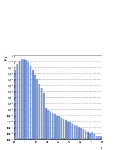
(a)

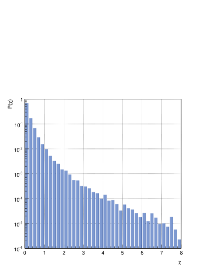
(b)

Figure 8: Frequency distribution of models with mean chirality $\chi$, as defined in (43), for the present $\mathbb{Z}_{6}$ case (a) to be compared with the result for $\mathbb{Z}_{2}\!\times\!\mathbb{Z}_{2}$ (b).

The inclusion of random samples of all possible stack sizes, weighted according to (38), leads to a frequency distribution as displayed in Figure 8(a). Until a value of $\chi\approx 2.8$ the contribution from models with more than eight stacks dominates. For these models the chirality is smaller on average, since the $AAB$ geometry, which allows for solutions with high chirality is no longer possible.

The distribution is quite different from what has been found for the $\mathbb{Z}_{2}\!\times\!\mathbb{Z}_{2}$ orbifold. In that case a general scaling behaviour was discovered, that has been conjectured in [10] based on a saddle point approximation. The chirality distribution, displayed in Figure 8(b), scales to a quite good approximation as $P(\chi)\sim e^{-3\sqrt{\chi}}$. In the present case the behaviour is different, especially because the distribution has two parts that scale differently. The first part goes roughly like $e^{-(\chi^{2})}$, while the second part scales like $e^{-\chi}$.

6.5 Standard model configurations

In the following we are going to focus our analysis on a special subclass of models, namely those which contain the gauge group and the chiral matter content of the standard model. To be precise, we should speak about the MSSM here, since all our models are $\mathcal{N}=1$ supersymmetric.

In order to simplify the analysis we use the term “standard model” in a very broad sense. In this section a standard model refers to a consistent solution which contains at least the gauge group and the chiral matter content of the MSSM. This means that there always exists a hidden sector, containing additional gauge groups and chiral matter. This is actually not necessarily bad for phenomenology, since in the end we need a mechanism to break supersymmetry, which can be nicely accomplished using a mediation through hidden sector fields.

Concerning so–called “chiral exotics”, i.e. matter that transforms non trivially under one of the gauge groups of the standard model, we will distinguish three cases to make our results comparable with the literature. Case (i) will have no restrictions on exotic matter at all. In case (ii) we forbid all exotic matter with the exception of bifundamental representations of the $SU(2)$ group of the standard model and an additional $U(1)$. These models are those that have been considered in [22] and might be of phenomenological relevance, since the bifundamentals can be interpreted as supersymmetric Higgs particles. However, since they do not transform under the same $U(1)$ as the weak doublets, it should be expected that the Yukawa couplings will be non–standard. In the most restrictive case (iii) we do not allow for any exotic matter at all.

As has been shown in [22], standard model configurations can only occur if the number of stacks is five or greater. The maximum number of stacks is nine, since models with more stacks do not support an $SU(3)$ gauge group. To simplify the analysis we will restrict ourselves to a special type of embedding of the standard model gauge group and chiral matter, namely the one introduced in Section 3.5.

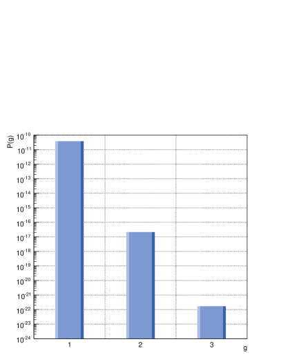
(a)

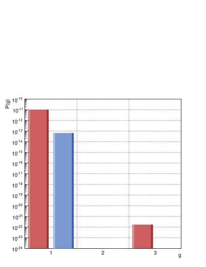
(b)

Figure 9: Distributions of the probability to find models with the gauge group of the standard model and $g$ generations of the chiral matter content. Figure (a) shows the results without any restrictions on chiral exotics, while in (b) the amount of bifundamental matter has been restricted either to maximally one pair transforming in the $SU(2)$ of the standard model (red bars on the left) or to no additional chiral matter at all (blue bars on the right).

6.5.1 Number of generations

At this point we leave the number of generations of quarks and leptons as a free parameter. In Figure 9 the frequency distribution of standard models with different numbers of families is shown. In Figure 9(a) we allowed all solutions with the gauge group and the chiral matter content of the standard model, while in Figure 9(b) we imposed additional constraints to exclude models with chiral exotics, as outlined above.

Models with more then two generations have only been found in the cases (i) and (ii), which allow for some amount of non–standard matter. In particular, there are $\approx 5.7\times 10^{6}$ solutions with three generations. These models all contain five stacks of branes and are of type (ii), containing one pair of bifundamental matter that transforms in the $SU(2)$ of the standard model gauge group and the $U(1)$ coming from the additional fifth brane. The models are of a type similar to the ones described in [22] and contain those as special cases. We also confirm the statement of that work, that such models can only exist for the $AAA$ geometry.

6.5.2 Spectra

As already mentioned above, we find the spectrum described in [22]. It can be described by the following cycles for the five brane stacks,

$$\pi_{a} = \frac{1}{2}\left(\rho_{1}+\rho_{2}+\varepsilon_{1}-2\tilde{\varepsilon}_{1}-2\varepsilon_{2}+\tilde{\varepsilon}_{2}+\varepsilon_{5}-2\tilde{\varepsilon}_{5}\right),$$

$$\pi_{b} = \frac{1}{2}\left(\rho_{1}+\rho_{2}-\varepsilon_{1}+2\tilde{\varepsilon}_{1}-2\varepsilon_{2}+\tilde{\varepsilon}_{2}-\varepsilon_{5}+2\tilde{\varepsilon}_{5}\right),$$

$$\pi_{c} = \frac{1}{2}\left(\rho_{1}+\rho_{2}+3\varepsilon_{2}-3\tilde{\varepsilon}_{2}-\varepsilon_{4}-\tilde{\varepsilon}_{4}+\varepsilon_{5}+\tilde{\varepsilon}_{5}\right),$$

$$\pi_{d} = \frac{1}{2}\left(\rho_{1}+\rho_{2}-\varepsilon_{1}+2\tilde{\varepsilon}_{1}+2\varepsilon_{2}-\tilde{\varepsilon}_{2}-\varepsilon_{5}+2\tilde{\varepsilon}_{5}\right),$$

$$\pi_{e} = \frac{1}{2}\left(\rho_{1}+\rho_{2}+3\varepsilon_{2}-3\tilde{\varepsilon}_{2}+\varepsilon_{4}+\tilde{\varepsilon}_{4}-\varepsilon_{5}-\tilde{\varepsilon}_{5}\right).$$

The chiral spectrum is given in Table 4.

$$\begin{array}[]{|l|l|c|r|r|r|r|r|r|}\hline\cr\text{matter}&\text{intersection}&SU(3)_{a}\times SU(2)_{b}&Q_{a}&Q_{b}&Q_{c}&Q_{d}&Q_{e}&Q_{Y}\\ \hline\cr Q_{L}&I_{ab^{\prime}}=-3&(\overline{\mathbf{3}},\mathbf{2})&-1&-1&0&0&0&\frac{1}{6}\\ U_{R}&I_{ac}=3&(\mathbf{3},\mathbf{1})&1&0&-1&0&0&-\frac{2}{3}\\ D_{R}&I_{ac^{\prime}}=3&(\mathbf{3},\mathbf{1})&1&0&1&0&0&\frac{1}{3}\\ L&I_{bd^{\prime}}=3&(\mathbf{1},\mathbf{2})&0&1&0&1&0&-\frac{1}{2}\\ E_{R}&I_{cd}=3&(\mathbf{1},\mathbf{1})&0&0&1&-1&0&1\\ N_{R}&I_{cd^{\prime}}=-3&(\mathbf{1},\mathbf{1})&0&0&-1&-1&0&0\\ \hline\cr&I_{be}=3&(\mathbf{1},\mathbf{2})&0&1&0&0&-1&0\\ &I_{be^{\prime}}=3&(\mathbf{1},\mathbf{2})&0&1&0&0&1&0\\ \hline\cr\end{array}$$

Table 4: Chiral spectrum of one of the models with gauge group $SU(3)\times SU(2)\times U(1)^{5}$ that contains the chiral matter spectrum of the standard model. $Q_{Y}$ is the hypercharge, realised as a combination of all $U(1)$ factors. Intersection numbers that are not listed are zero. Note the explicit appearance of right–handed neutrinos ($N_{R}$).

In addition we find several variations of this configuration, all very similar in structure. The difference between all of these models is only given by the explicit realisation in terms of wrapping numbers. Furthermore the left–handed quarks might be realised through $I_{ab}=-3$ and $I_{ab^{\prime}}$ vanishing. However, this is only a technical detail and does not change the general setup of the model, which can therefore be seen as the unique construction to obtain a standard model spectrum on this particular orbifold.

6.5.3 Hidden sector

The hidden sector of the standard models is generically very small. This is in sharp contrast to the models on the $\mathbb{Z}_{2}\!\times\!\mathbb{Z}_{2}$ orbifold, where we found quite large hidden sectors with a distribution of gauge groups that turned out to be almost identical to the distribution in the full set of models [11]. The reason for this is that the number of stacks in the present case is restricted to a maximum of nine, and the tadpole equations limit the total rank to be lower than or equal to twelve (cf. Section 6.3.1).

If we restrict our attention to the group of models which are most interesting from a phenomenological point of view, namely the three generation models, we find that they only occur in configurations with five stacks of branes. In this case the “hidden sector” consists only of one $U(1)$ gauge factor and in addition we always have chiral matter transforming under this $U(1)$ and the $SU(2)$ group of the standard model.

7 Conclusions and outlook

In this work we have performed a complete analysis of type II intersecting D–brane models on the $T^{6}/\mathbb{Z}_{6}$ orientifold. We found that there exist $3.4\times 10^{28}$ solutions in total, out of which $5.7\times 10^{6}$ contain the gauge group and chiral matter content of the standard model. We therefore obtained a probability of $1.7\times 10^{-22}$ to find an MSSM–like vacuum, a number considerably lower then the value of $10^{-9}$ that has been calculated in the case of $\mathbb{Z}_{2}\!\times\!\mathbb{Z}_{2}$ orientifolds in [11].

The distribution of gauge groups and chiral matter in the full set of solutions has been analysed and we compared the results with those from a similar study of $\mathbb{Z}_{2}\!\times\!\mathbb{Z}_{2}$ models. Similar frequency distributions of single gauge group factors have been found, but the distribution of the total rank of the gauge group and of the chiral matter content are quite different. This has been explained by the fact that the branes considered in this work are actually fractional branes that wrap not only torus cycles, but generically also exceptional cycles around fixed points of the orbifold. Since there exists a large number of possibilities to combine these cycles, the number of solutions is considerably increased and the statistical distributions are altered significantly compared to the $\mathbb{Z}_{2}\!\times\!\mathbb{Z}_{2}$–case, in which fractional branes have not been considered.

To obtain the full statistics, a method based on the choice of randomly chosen subsets of the full solution space has been used. Therefore our results are not exact, but come with a statistical error, which is however very small and always below 1%.

Concerning future directions, it would certainly be very interesting to compare our results with other string compactifications that use different setups. In particular a better comparison with the heterotic landscape [20, 21] and the statistics of M–theory vacua [32] would be desirable. Comparing our results with the extensive analysis of Gepner models [17, 18, 19] would also be very interesting, although in this case the analysis is complicated by the fact that we are considering only one particular geometry over a wide range of (untwisted) moduli here, whereas the analysis in the works cited above has been done for a very large set of different geometries at a particular point in moduli space. Moreover the Gepner model statistic considers only models which resemble the standard model gauge group. Nevertheless we hope to come back to this issue in the future.

On a more technical level, our analysis of solutions that resemble properties of the standard model could be improved. Since we discussed only one possible embedding there might be more possible realisations with interesting phenomenological features, although most of the embeddings used in different contexts will not work due to the fact that the number of symmetric and antisymmetric representations has to be equal.

Another extension of this work concerns the inclusion of fluxes. In a naive way this can be done easily by considering a lowered orientifold charge, as this would generically be the effect of switching on three–form flux. However, to incorporate the most general NSNS– and RR–fluxes into an orientifold setup, it seems very likely that the simple mathematical formalism used in this article has to be considerably extended.

- [1] D. Lüst, Intersecting brane worlds: A path to the standard model?, Class. Quant. Grav. 21 (2004) S1399–1424, [hep-th/0401156].
- [2] R. Blumenhagen, M. Cvetic, P. Langacker, and G. Shiu, Toward realistic intersecting D-brane models, Ann. Rev. Nucl. Part. Sci. 55 (2005) 71–139, [hep-th/0502005].
- [3] R. Blumenhagen, B. Körs, D. Lüst, and S. Stieberger, Four-dimensional string compactifications with D-branes, orientifolds and fluxes, hep-th/0610327.
- [4] W. Lerche, D. Lüst, and A. N. Schellekens, Chiral four-dimensional heterotic strings from selfdual lattices, Nucl. Phys. B287 (1987) 477.
- [5] M. R. Douglas, The statistics of string / M theory vacua, JHEP 05 (2003) 046, [hep-th/0303194].
- [6] J. Kumar, A review of distributions on the string landscape, Int. J. Mod. Phys. A21 (2006) 3441–3472, [hep-th/0601053].
- [7] M. R. Douglas and S. Kachru, Flux compactification, hep-th/0610102.
- [8] F. Denef, M. R. Douglas, and S. Kachru, Physics of String Flux Compactifications, hep-th/0701050.
- [9] B. S. Acharya and M. R. Douglas, A finite landscape?, hep-th/0606212.
- [10] R. Blumenhagen, F. Gmeiner, G. Honecker, D. Lüst, and T. Weigand, The statistics of supersymmetric D-brane models, Nucl. Phys. B713 (2005) 83–135, [hep-th/0411173].
- [11] F. Gmeiner, R. Blumenhagen, G. Honecker, D. Lüst, and T. Weigand, One in a billion: MSSM-like D-brane statistics, JHEP 01 (2006) 004, [hep-th/0510170].
- [12] F. Gmeiner, Standard model statistics of a type II orientifold, Fortsch. Phys. 54 (2006) 391–398, [hep-th/0512190].
- [13] F. Gmeiner and M. Stein, Statistics of SU(5) D-brane models on a type II orientifold, Phys. Rev. D73 (2006) 126008, [hep-th/0603019].
- [14] F. Gmeiner, Gauge sector statistics of intersecting D-brane models, Fortsch. Phys. 55 (2007) 111–160, [hep-th/0608227].
- [15] J. Kumar and J. D. Wells, Surveying standard model flux vacua on , JHEP 09 (2005) 067, [hep-th/0506252].
- [16] M. R. Douglas and W. Taylor, The landscape of intersecting brane models, JHEP 01 (2007) 031, [hep-th/0606109].
- [17] T. P. T. Dijkstra, L. R. Huiszoon, and A. N. Schellekens, Chiral supersymmetric standard model spectra from orientifolds of Gepner models, Phys. Lett. B609 (2005) 408–417, [hep-th/0403196].
- [18] T. P. T. Dijkstra, L. R. Huiszoon, and A. N. Schellekens, Supersymmetric standard model spectra from RCFT orientifolds, Nucl. Phys. B710 (2005) 3–57, [hep-th/0411129].
- [19] P. Anastasopoulos, T. P. T. Dijkstra, E. Kiritsis, and A. N. Schellekens, Orientifolds, hypercharge embeddings and the standard model, Nucl. Phys. B759 (2006) 83–146, [hep-th/0605226].
- [20] K. R. Dienes, Statistics on the heterotic landscape: Gauge groups and cosmological constants of four-dimensional heterotic strings, Phys. Rev. D73 (2006) 106010, [hep-th/0602286].
- [21] O. Lebedev et al., A mini-landscape of exact MSSM spectra in heterotic orbifolds, Phys. Lett. B645 (2007) 88–94, [hep-th/0611095].
- [22] G. Honecker and T. Ott, Getting just the supersymmetric standard model at intersecting branes on the -orientifold, Phys. Rev. D70 (2004) 126010, [hep-th/0404055].
- [23] D.-E. Diaconescu, M. R. Douglas, and J. Gomis, Fractional branes and wrapped branes, JHEP 02 (1998) 013, [hep-th/9712230].
- [24] D.-E. Diaconescu and J. Gomis, Fractional branes and boundary states in orbifold theories, JHEP 10 (2000) 001, [hep-th/9906242].
- [25] K. R. Dienes and M. Lennek, Fighting the floating correlations: Expectations and complications in extracting statistical correlations from the string theory landscape, Phys. Rev. D75 (2007) 026008, [hep-th/0610319].
- [26] D. Bailin and A. Love, Towards the supersymmetric standard model from intersecting D6-branes on the Z’(6) orientifold, Nucl. Phys. B755 (2006) 79–111, [hep-th/0603172].
- [27] F. Gmeiner and G. Honecker. Work in progress.
- [28] M. Klein and R. Rabadan, D = 4, N = 1 orientifolds with vector structure, Nucl. Phys. B596 (2001) 197, [hep-th/0007087].
- [29] R. Blumenhagen, L. Görlich, and T. Ott, Supersymmetric intersecting branes on the type IIA orientifold, JHEP 01 (2003) 021, [hep-th/0211059].
- [30] E. Witten, An SU(2) anomaly, Phys. Lett. B117 (1982) 324–328.
- [31] A. M. Uranga, D-brane probes, RR tadpole cancellation and K-theory charge, Nucl. Phys. B598 (2001) 225–246, [hep-th/0011048].
- [32] B. S. Acharya, F. Denef, and R. Valandro, Statistics of M theory vacua, JHEP 06 (2005) 056, [hep-th/0502060].