The 5-D Choptuik critical exponent and holography

Abstract

Recently, a holographic argument was used to relate the saturation exponent, $\gamma_{BFKL}$, of four-dimensional Yang-Mills theory in the Regge limit to the Choptuik critical scaling exponent, $\gamma_{5d}$, in 5-dimensional black hole formation via scalar field collapse [1]. Remarkably, the numerical value of the former agreed quite well with previous calculations of the latter. We present new results of an improved calculation of $\gamma_{5d}$ with substantially decreased numerical error. Our current result is $\gamma_{5d}=0.4131\pm 0.0001$, which is close to, but not in strict agreement with, the value of $\gamma_{BFKL}=0.409552$ quoted in [1].

The critical behaviour exhibited by gravitational collapse to black holes, first discovered by Choptuik [2] (see [3, 4] for reviews), is a small scale, strong gravitational field effect that is by now well understood at the qualitative level. As well, key physical quantities such as the associated critical solution and scaling exponents have been calculated numerically. Precise analytic derivations of these quantities are still, to the best of our knowledge, lacking.

Recently, intriguing holographic arguments were used to relate the strong field gravitational scaling behaviour in spherically symmetric scalar field collapse in five space-time dimensions to scaling in a suitable, 4-D weakly coupled gauge theory [1]. Specifically, it was conjectured that exponential growth of the scattering amplitude for two hadrons in the one-pomeron exchange approximation corresponded via a holographic mapping to the exponential growth away from the critical solution that leads to Choptuik scaling in five dimensions. Thus, it was argued, the BFKL scaling exponent $\gamma_{BFKL}$ should equal the 5-dimensional Choptuik scaling exponent $\gamma_{5d}$.

As shown by the authors of [1], a numerical calculation of the BFKL scaling exponent yields the value $\gamma_{BFKL}=0.409552$. On the other hand, the most accurate previous calculation yields a 5-D Choptuik scaling exponent of: $\gamma_{5d}=0.412\pm 0.004$ [5]. A somewhat lower result , namely $0.408$, was reported in [6], but with an error of $\pm 0.008$. The apparent agreement between $\gamma_{BFKL}$ and $\gamma_{5d}$ provides startling support for the conjecture relating 5d gravity to pomeron exchange in 4d Yang-Mills theory, and for the general validity of the holography hypothesis.

The purpose of this note is to present the results of a more accurate calculation of $\gamma_{5d}$ and the related echoing period $\Delta_{5d}$. Recall that the Choptuik scaling exponent is most directly observed in the simple scaling law obeyed by the horizon radius near criticality [2]

$$R_{AH}\propto(a-a_{*})^{\gamma}.$$ (1)

where $R_{AH}$ is the horizon radius on formation, $a$ is a parameter describing the initial data whose critical value $a_{*}$ separates initial data that lead to blackhole formation from those that lead to dispersal of the scalar field. The echoing period $\Delta_{5d}$ derives from the discrete self-similarity of the critical solution, and can be extracted from the periodicity of the critical scalar field solution:

$$\chi(r,t)=\chi\left(re^{\Delta_{5d}},te^{\Delta_{5d}}\right)$$ (2)

The new values we obtain for these quantities are

$$\gamma_{5d}=0.4131\pm 0.0001\hskip 25.0pt\Delta_{5d}=3.225\pm 0.003.$$ (3)

These results are consistent within error with previous calculations, but $\gamma_{5d}$ no longer agrees precisely with $\gamma_{BFKL}$. Nevertheless, given the uncertainties in the calculation of $\gamma_{BFKL}$, a discrepancy of this order (less than 1$\%$) is perhaps not surprising[7].

We now describe how (3) was obtained. Our formalism and code are basically the same as that used in [5], which in turn was based on the analysis of [8]. A couple of crucial changes have permitted the increase in the accuracy by a factor of about twenty.

The calculation can generically be formulated in terms of Einstein gravity in $D$ space-time dimensions minimally coupled to a massless scalar field[8]:

$$S^{(D)} = {1\over 16\pi G^{(D)}}\int d^{D}x\sqrt{-g^{(D)}}R(g^{(D)})$$ (4)

$$-\int d^{D}x\ \sqrt{-g^{(D)}}|\partial\chi|^{2}.$$

Spherical symmetry is imposed by requiring:

$$ds^{2}_{(D)} = \bar{g}_{\alpha\beta}dx^{\alpha}dx^{\beta}+r^{2}(x^{\alpha})d\Omega_{(D-2)},$$

$$\chi = \chi(x^{\alpha})$$ (5)

where $d\Omega_{(D-2)}$ is the metric on $S^{D-2}$ and $\alpha,\beta=1,2$. A relatively simple set of equations can be obtained by the following field redefinition, which is motivated by 2-dimensional dilaton gravity [8, 9]:

$$\phi := {D-2\over 8(D-3)}\left({r\over l}\right)^{D-2},$$ (6)

$$g_{\alpha\beta} := \phi^{(D-3)/(D-2)}\ \bar{g}_{\alpha\beta},$$ (7)

where $r$ is the optical scalar and $\phi$ is proportional to the area of a $(D-2)$-sphere at fixed radius $r$.

We go to double null coordinates first introduced by Garfinkle [10]:

$$ds^{2}=-2lg(u,v)\phi^{\prime}(u,v)dudv$$ (8)

in which the relevant field equations take the form:

$$\dot{\phi}^{\prime}=-{D-3\over 2}\left({r\over l}\right)^{D-3\over D-2}g\phi^{\prime}$$ (9)

$${g^{\prime}\phi^{\prime}\over g\phi}=32\pi(\chi^{\prime})^{2}$$ (10)

$$(\phi\chi^{\prime})^{\cdot}+(\phi\dot{\chi})^{\prime}=0,$$ (11)

where the prime and dot denote $v$ and $u$ derivatives, respectively. We henceforth restrict attention to five dimensions by setting $D=5$, in which case $r\propto\phi^{1/3}$.

The general method we use starts with the choice of a one parameter family of initial data for the scalar field $\chi$. Coordinate invariance allows the initial value of $\phi$ to be chosen arbitrarily, while the metric component $g$ is obtained by integrating the constraint Eq.(10). We then evolve the data using the remaining dynamical equations (9) and (11) until either a horizon forms, or the field disperses. Horizon formation is signalled by the vanishing of the null expansion scalar, which for spherically symmetric geometries is given by:

$$AH\equiv{g}^{\alpha\beta}\partial_{\alpha}\phi\partial_{\beta}\phi.$$ (12)

This calculation is repeated for different values of some parameter, $a$, describing the initial data in order to determine the critical value, $a_{*}$, separating black hole final states from dispersed final states. Once $a_{*}$ is determined, we calculate the horizon radius at formation, $R_{AH}$, for a wide range of super-critical values of $a$ near $a_{*}$ and then plot $\ln(R_{AH})$ vs $\ln(a-a_{*})$. This generically yields an (almost) straight line (see Figure 1) from which the scaling exponent and echoing period can be obtained by fitting the ln-ln plot to the following 5 parameter function:

$$\ln\left(R_{AH}\right)=c_{0}+\gamma_{5d}\ln(a-a_{*})+c_{1}\sin\left[\left({2\pi\over\delta_{5d}}\right)\ln(a-a_{*})+c_{2}\right],$$ (13)

where $\{c_{0},c_{1},c_{2}\}$ are family dependent constants. The periodic deviations from a line in the ln-ln plot yield the echoing period via the relation $\Delta_{5d}=2\gamma_{5d}\delta_{5d}$ [11]. A more accurate value for $\Delta$ can be obtained by measuring the period of oscillations of the matter field at the origin as a function of $-ln(u_{*}-u)$, where $u_{*}$ is the $a=a_{*}$ value of the coordinate $u$ at collapse (See Figure 2).

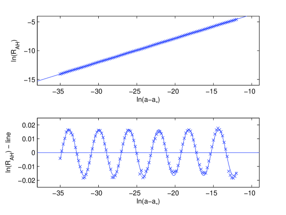
Figure 1: Plot of $ln(R_{AH})$ vs $ln(a-a_{*})$ (top graph). The value of $a_{*}$ was adjusted within a small range in order to increase the quality of the fit and to determine the error in $\gamma_{5d}$. In the bottom graph, the linear portion of the fit is subtracted from $ln(R_{AH})$. The residuals are well described by a sine wave (solid curve) and clearly show the oscillation expected due to the discrete self-similarity of the critical solution.

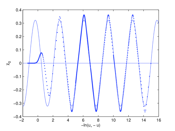
Figure 2: Plot of the matter field at the origin vs $-ln(u_{*}-u)$. The value of $u_{*}$ was adjusted within a small range to increase the quality of the fit and to determine the uncertainty of the best estimate of the self-similarity period. $\Delta_{5d}$ is determined by calculating the period of the oscillation (the solid line represents the best fit to the data.)

Our specific numerical scheme used a $v$ (‘space’) discretization to obtain a set of coupled ODEs:

$$h(u,v)\rightarrow h_{i}(u)\hskip 25.0pt\phi(u,v)\rightarrow\phi_{i}(u)$$ (14)

where $i=0,\ldots,(N-1)$ specifies the $v$ grid and $h=\chi+2\phi\chi^{\prime}/\phi^{\prime}$. Initial data for these two functions were prescribed on a constant $v$ slice, from which the function $g(u,v)$ was constructed.

In all cases we started with Gaussian initial data

$$\chi(u=0,\phi)=a\phi^{2/3}\ {\rm exp}\left[-\left(\ {\phi-\phi_{0}\over\sigma}\right)^{2}\right].$$ (15)

The initial scalar field configuration $\chi(u=0,\phi)$ is most conveniently specified as a function of $\phi$ rather than $r$. (Recall that $\phi\propto r^{3}$.) The value of the dilaton field at each grid point on the initial surface was chosen for simplicity to be:

$$\phi_{i}(u=0,v)=(i+1)\Delta v,$$ (16)

where $\Delta v$ is the initial grid spacing. The initial values of the other functions were determined in terms of the above by computing the integrals $g_{i}$ using Euler’s method for equally spaced points.

The results in Eq.(3) were obtained with an initial spacing $\Delta v=0.0012$ along with an initial grid size of $N=2048$. We further verified these results by performing calculations at several smaller grid sizes (with proportionately larger initial grid spacings) (See Table 1). To the stated error, the scaling exponent was independent of initial grid size, while echoing period $\Delta_{5d}$ varied between about 3.223 and 3.226. This determined the error bars on $\Delta_{5d}$ given in Eq.(3).

Initial Grid Size	Initial Grid Spacing	$\gamma_{5d}$	$\Delta_{5d}$
$512$	$0.0048$	$0.4130\pm 0.0001$	$3.2264\pm 0.0005$
$800$	$0.003072$	$0.4130\pm 0.0001$	$3.2230\pm 0.0006$
$1024$	$0.0024$	$0.4131\pm 0.0001$	$3.2223\pm 0.0006$
$1536$	$0.0016$	$0.4131\pm 0.0001$	$3.2264\pm 0.0004$
$2048$	$0.0012$	$0.4131\pm 0.0001$	$3.2246\pm 0.0005$

Table 1: Choptuik 5-d critical exponent and echoing period calculated with varying initial grid sizes.

Evolution in the ‘time’ variable $u$ was performed using the $4^{th}$ order Runge-Kutta method. The general scheme is similar to that used in [12], together with some refinements used in [10]. This procedure was also used for the $3-$dimensional collapse calculations in [13]. The accuracy of the calculation was improved by decreasing the time steps as the calculation progressed according to the formula:

$$\Delta u=\Delta u_{0}\left(1-0.999\exp\left[-\left({u_{*}-u\over 0.1}\right)^{2}\right]\right),$$ (17)

where $\Delta u_{0}=0.001$ is the initial time step spacing and $u_{*}$ is the estimated value of the coordinate $u$ of the critical solution. Further improvements in accuracy were made by decreasing the value of $\Delta u_{0}$ periodically during the calculation, or once apparent horizon formation commenced, i.e., once the function $AH(\phi)$ developed an extremum. Time steps ranged from $\Delta u=10^{-3}$ at the beginning of the calculation to about $\Delta u=10^{-11}$ near the end.

The boundary conditions at fixed $u$ are

$$\phi_{k}=0\hskip 15.0ptg_{k}=1,$$ (18)

where $k$ is the index corresponding to the position of the origin $\phi=0$. All grid points $0\leq i\leq k-1$ correspond to ingoing rays that have reached the origin and are dropped from the grid. The boundary conditions are equivalent to $r(u,u)=0$, $g|_{r=0}=g(u,u)=1$. Notice that for our initial data, $\phi_{k}$ and hence $h_{k}$, are initially zero, and therefore remain zero at the origin because of Eq.(11).

The most significant improvement in the numerical code over [5], involved systematically decreasing the grid spacing $\Delta v$ using a method similar to that of [10]. At regular intervals in $ln(u_{*}-u)$, the exterior half of the gridpoints were discarded. The number of gridpoints was then restored by using a $4^{th}$ order Lagrange interpolation between the remaining grid points, thereby doubling the resolution. Typically, by the end of the calculation the grid spacing was decreased to approximately $10^{-6}$. This allowed the accuracy of the horizon position to be maintained over the entire ln-ln plot and reduced significantly the overall uncertainty in $\gamma_{5d}$.

At each $u$ step, a check was made to see if an apparent horizon had formed by observing the function $AH$ in Eq.(12) whose vanishing signals the formation of an apparent horizon. For each run of the code with fixed parameters $a$, $\sigma$, and $\phi_{0}$, this function was scanned from larger to smaller radial values after each Runge-Kutta iteration for the presence of an apparent horizon. In the sub-critical case, all the radial grid points reached zero without detection of an apparent horizon, which signals pulse reflection. In the super-critical case, black hole formation was signalled by the vanishing of $AH$ at some finite radius. Since the code crashes when $AH<0$, so the the time evolution was slowed down as $AH\rightarrow 0^{+}$ in order to obtain the most accurate estimate of the apparent horizon position. For any given run, the apparent horizon position ($R_{MIN}$) was assigned the value of the grid point for which $AH$ reached a minimum during the last surviving iteration.

For our initial runs we fixed the location and width of the Gaussian initial data to be $\phi_{0}=1$ and $\sigma=0.3$, respectively. We then varied the amplitude $a$ to determine the critical amplitude $a_{*}$ via a binary search. The code was written using double precision in C thus, the binary search was terminated when $a_{*}$ was determined to $15$ digits. We then did runs in the super-critical region $a>a_{*}$ to determine the dependence of the horizon radius $R_{AH}$ on the amplitude. It was found that numerical error would introduce noise in the ln-ln plot for the runs closest to $a_{*}$ and so only super-critical runs for which $(a-a_{*})/a_{*}>10^{-13}$ were fitted to determine $\gamma_{5d}$. To improve the quality of the fit Eq. (13), the value of $a_{*}$ was adjusted within the range of values between super-critical and sub-critical collapse obtained during the binary search. The error associated with $\gamma_{5d}$ represents the range of fit results when $a_{*}$ is adjusted within that range. The universality of the critical solution was verified by starting runs $a=a_{*}$ and varying the width and center of the initial data profile. As shown in Table 2, the results for $\gamma_{5d}$ agreed within error in all cases.

Critical parameter	$\gamma_{5d}$
$a$	$0.4131\pm 0.0001$
$\sigma$	$0.4131\pm 0.0003$
$\phi_{0}$	$0.4133\pm 0.0004$

Table 2: Choptuik scaling exponent in 5 dimensional super-critical collapse. We verified the universality of the critical solution by varying the width and center of the initial data profile. The scaling constants calculated by varying $\sigma$ and $\phi_{0}$ are in agreement with the results obtained by varying the amplitude of the initial pulse. Universality was tested at an initial grid size of $2048$.

To summarize, we have obtained fairly accurate values for the Choptuik scaling exponent and echoing period in spherically symmetric scalar field collapse in five dimensions:

$$\gamma_{5d}=0.4131\pm 0.0001\hskip 25.0pt\Delta_{5d}=3.225\pm 0.003.$$ (19)

These results agree within error with all previous calculations, but the value of $\gamma_{5d}$ does differ somewhat from $\gamma_{BFKL}$. The discrepancy is small but potentially significant. It should, however, be kept in mind that the value calculated in [1] is strictly speaking exact only in the asymptotic high energy region and it is not yet completely clear where this region begins. Hence there may be corrections due to the usual running of the strong coupling constant, saturation and other effects [7]. Thus although the proposed holographic connection between $\gamma_{BFKL}$ and $\gamma_{5d}$ is compelling, more work is required in order to confirm its validity.

Acknowledgements
This work was supported in part by the Natural Sciences and Engineering Research Council of Canada. We are thankful to L. Alverez-Gaume and D. Garfinkle for useful discussions and encouragement.

References

- [1] L. Álvarez-Gaumé, C. Gómez and M. A. Vázquez-Mozo, “Scaling Phenomena in Gravity from QCD”, hep-th/0611312 (2006).
- [2] M. Choptuik, Phys. Rev. Lett. 70, 9 (1993).
- [3] C. Gundlach, Phys. Rep. 376, 339 (2003).
- [4] L. Lehner, Class. Quantum Grav. 18, R25 (2001).
- [5] J. Bland, B. Preston, M. Becker, G. Kunstatter and V. Husain, Class. Quantum Grav. 22, 5355 (2005).
- [6] E. Sorkin and Y. Oren, Phys. Rev. D7, 124005 (2005).
- [7] L. Alvarez-Gaume, private communication.
- [8] M. Birukou, V. Husain, G. Kunstatter, E. Vaz and M. Olivier, Phys. Rev. D65, 104036 (2002); V. Husain, G. Kunstatter, B. Preston and M. Birukou, Class. Quantum Grav. 20, L23 (2003).
- [9] J. Gegenberg, D. Louis-Martinez and G. Kunstatter, Phys. Rev. D51, 1781 (1995); D. Louis-Martinez and G. Kunstatter, Phys. Rev. D52, 3494 (1995).
- [10] D. Garfinkle, Phys. Rev. D51, 5558 (1995).
- [11] S. Hod and T. Piran, Phys. Rev. D55, 440 (1997).
- [12] D. Goldwirth and T. Piran, Phys. Rev. D36, 3575 (1987).
- [13] V. Husain and M. Olivier, Class. Quantum Grav. 18, L1 (2001).