Cosmological Perturbations in Non-Commutative Inflation

Abstract

We compute the spectrum of cosmological perturbations in a scenario in which inflation is driven by radiation in a non-commutative space-time. In this scenario, the non-commutativity of space and time leads to a modified dispersion relation for radiation with two branches, which allows for inflation. The initial conditions for the cosmological fluctuations are thermal. This is to be contrasted with the situation in models of inflation in which the accelerated expansion of space is driven by the potential energy of a scalar field, and in which the fluctuations are of quantum vacuum type. We find that, in the limit that the expansion of space is almost exponential, the spectrum of fluctuations is scale-invariant with a slight red tilt. The magnitude of the tilt is different from what is obtained in a usual inflationary model with the same expansion rate during the period of inflation. The amplitude also differs, and can easily be adjusted to agree with observations.

I Introduction

Various approaches to quantum gravity indicate that the effective field theory which emerges below the cutoff scale will be non-commutative. For example, in the context of string theory, one of the reasons for non-commutativity is that the basic objects which underlie the quantum theory are strings rather than point particles. A concrete formulation of this non-commutativity comes from the “stringy space-time uncertainty relation” of Yoneya ; Li . In the matrix theory approach to non-perturbative string theory, spatial coordinates arise in a certain limit from matrices which are non-commuting Jevicki ; BFSS ; IKKT . This leads to space-space non-commutativity.

The most promising arena to probe the fundamental non-commutativity of space-time on microscopic scales is cosmology. The reason is that, according to our present understanding, the seeds for the currently observed structure of the universe on large scales were laid down in the very early universe when the length scales which we probe today in cosmology were microscopic and thus subject to the modifications in the dynamics which arise due to the non-commutativity.

The inflationary universe scenario is the current paradigm for early universe cosmology Guth (see also Starob1 ; Sato ; Brout ). According to this scenario, the universe experiences a period of accelerated expansion in its early stages. Often, the expansion is close to exponential, or it is described by the scale factor $a(t)$ expanding as a large power $p>1$ of time t. This accelerated expansion leads to the possibility of a causal structure formation scenario, as first discussed in Mukh1 (see also Starob2 ; Press ; Sato ). Figure 1 provides a space-time sketch illustrating the basic idea. During the period of acceleration, fixed comoving scales are stretched beyond the Hubble radius $H^{-1}$. Fluctuations on these scales can become the seeds for the presently observed large-scale structure and the anisotropies in the cosmic microwave background.

By the same argument, however, we can argue RHBrev1 that fluctuations on currently observed scales had a wavelength during the early stages of inflation which was so small that effects of Planck-scale physics will be operative and leave an imprint on the initial evolution of the fluctuations, effects which are preserved until late times by the linear evolution of the fluctuations. Initial studies of effects of trans-Planckian physics on current observations in the context of inflationary cosmology made use of ad hoc modified dispersion relations for the fluctuation modes Martin . These initial studies were followed by specific investigations of the effects of space-space SSUR and space-time Ho non-commutativity. All of the works referenced in this paragraph were based on the current models of inflation in which it is assumed that inflation is driven by the potential energy of a scalar matter field. In this context, any pre-existing classical fluctuations at the beginning of the phase of inflation are red-shifted, leaving behind a quantum vacuum. Hence, it was postulated that the currently observed fluctuations are the result of the non-trivial evolution of quantum vacuum perturbations (see e.g. MFB for a comprehensive review of the theory of cosmological perturbations, and RHBrev2 for a pedagogical introduction).

Non-commutativity of space-time or space-space leads to deformed dispersion relations (see e.g. Kempf ). Whereas space-space non-commutativity introduces anisotropy into the dispersion relations, space-time non-commutativity leads to dispersion relations which preserve isotropy. In Joao1 a class of deformed dispersion relation for ordinary radiation resulting from space-time non-commutativity was studied. This dispersion relation has a maximal momentum, and it has two branches (two values of frequency for fixed momentum). In Joao2 it was pointed out that this dispersion relation makes it possible to obtain a period of inflation driven by non-commutative radiation. Typically, one obtains power-law inflation, inflation driven by the radiation itself. In Joao2 , an order of magnitude estimate of the amplitude of the resulting cosmological fluctuations was given. In this paper, we present a detailed study of the spectrum of cosmological perturbations in this model of non-commutative inflation. In contrast to the conventional models of inflation where the fluctuations are of quantum vacuum origin, in our model they are due to thermal fluctuations . In this aspect, our model has analogies with the “warm inflation” scenario warm in which the fluctuations are also of thermal origin.

The following Section provides a brief review of the non-commutative inflation scenario of Joao1 ; Joao2 . Section 3 gives a summary of the key equations which describe the evolution of cosmological fluctuations which we will make use of. In Section 4, we present the computation of the spectrum of scalar metric perturbations, based on thermal initial values for the fluctuations. We conclude with a brief discussion.

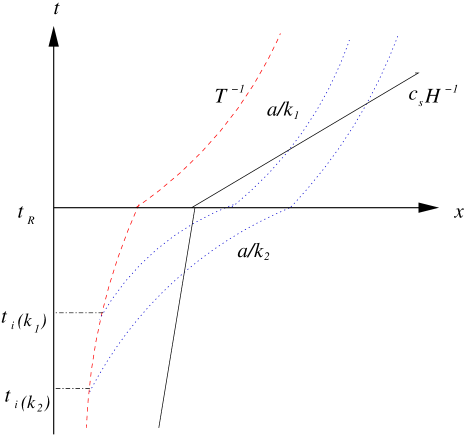
Figure 1: Space-time sketch depicting the expansion of fixed comoving scales in inflationary cosmology. The horizontal axis represents the physical distance, the vertical axis time. The time $t_{R}$ denotes the transition time between the inflationary phase and the radiation phase of standard cosmology. The curves corresponding to the physical wavelengths of two comoving scales with comoving wavenumbers $k_{1}$ and $k_{2}$ are labelled by their wavenumbers. The solid line indicates the sound horizon (up to an irrelevant constant equal to the Hubble radius), the dashed line is the thermal correlation length. Note that the slopes of these two curves are different.

II Non-Commutative Inflation

In the case of massless particles, the non-commutativity of space-time leads to modifications of the usual linear dispersion relation which take the form

$$E^{2}-p^{2}c^{2}f(E)^{2}\,=\,0\,$$ (1)

with

$$f(E)\,=\,1+(\lambda E)^{\alpha}\,.$$ (2)

In the above, $p$ and $E$ denote momentum and energy, respectively, $\alpha$ is a positive constant, and $\lambda$ is a length scale whose physical meaning is the following: solving (2) for the momentum $p$, we see immediately that for $\alpha\geq 1$ there is a maximal momentum $p_{max}$ whose value is determined by $\lambda$. For example, for $\alpha=1$ the maximal momentum is $p_{max}=1/(c\lambda)$.

For $\alpha>1$, there are two values of the energy $E$ for any momentum - the dispersion relation has two branches. On the upper branch, the energy increases as the momentum decreases, which is what happens when the universe expands. It is this property which is crucial in order to realize that modified dispersion relations with $\alpha>1$ can, at least for a certain range of values of $\alpha$, lead to inflation driven by ordinary radiation.

The modification of the dispersion relation leads to a deformed thermal spectrum Joao1 due to the changing density of states

$$\rho(E)\,=\,\frac{1}{\pi^{2}\hbar^{3}c^{3}}\frac{E^{3}}{e^{\beta E}-1}\frac{1}{f^{3}}\left|1-\frac{f^{\prime}E}{f}\right|\,,$$ (3)

where $\rho(E)$ denotes the energy density (per unit $E$) and $\beta$ is the inverse temperature . In the high energy limit, $f^{\prime}E/f\simeq\alpha$. The high energy Stephan-Boltzmann equation takes the form $\rho\propto T^{\gamma}$ with $1<\gamma<4$ where $\gamma=4$ for $\alpha=0$ and $\gamma=1$ for $\alpha\geq 1$.

The equation of state which follows from the modified dispersion relation is given by

$${\cal P}\,=\,\frac{1}{3}\int\frac{\rho(E)dE}{1-\frac{f^{\prime}E}{f}}\,,$$ (4)

where ${\cal P}$ stands for the pressure. This is approximated in the high energy limit by

$$w(\rho\rightarrow\infty)\,\simeq\,\frac{1}{3(1-\alpha)}\,,$$ (5)

where $w={\cal P}/\rho$ is the usual equation of state parameter. For $\alpha>1$, the equation of state parameter $w$ takes on negative values and it is possible to have inflationary expansion with $-1\leq w<-1/3$ for temperatures $T\gg 1/\lambda$.

The Friedmann and energy conservation equations are

$$\left(\frac{\dot{a}}{a}\right)^{2}\, = \,\frac{8\pi}{3M_{p}}\rho,$$ (6)

$$\dot{\rho}\, = \,-3\frac{\dot{a}}{a}(1+w)\rho$$

and its solutions are given for a constant equation of state parameter by

$$\rho\, \propto \,a^{-3(1+w)}\,\sim\,a^{-\frac{4-3\alpha}{1-\alpha}}$$

$$a(t)\, \propto \,t^{\frac{2}{3(1+w)}}\,\propto\,\eta^{\frac{2}{1+3w}}$$ (7)

These show power law inflation ($-1\leq w<-1/3$) for values of $\alpha$ in the range $4/3\leq\alpha<2$ . For $\alpha\simeq 4/3$ we have almost exponential inflation. Note that for $1<\alpha<4/3$, non-commutative radiation at $T\gg 1/\lambda$ behaves like phantom matter ($w<-1$). Inflation ends at time $t_{R}$ when there are no more excited states on the top branch of the dispersion relation.

III Key tools of the theory of cosmological perturbations

In this section we will list the key equations from the theory of cosmological perturbations which will be used. We work in longitudinal gauge in which the metric takes the form

$$ds^{2}\,=\,a^{2}[-(1+2\Phi)d\eta^{2}+(1-2\Psi)\gamma_{ij}dx^{i}dx^{j}]\,,$$ (8)

where $a(\eta)$ is the scale factor, $\eta$ being conformal time, and the functions $\Phi$ and $\Psi$ describe the scalar metric fluctuations and thus depend on space and time. At the linearized level, the perturbed Einstein equations can be written as MFB

$$3\mathcal{H}^{2}\Phi+3\mathcal{H}\Psi^{\prime}-\nabla^{2}\Psi=-4\pi Ga^{2}\delta{T^{0}}_{0},$$ (9)

$$(\mathcal{H}\Phi+\Psi^{\prime})_{,i}=4\pi Ga^{2}\delta{T^{0}}_{i},$$ (10)

$$[(2\mathcal{H}^{\prime}+\mathcal{H})\Phi+\mathcal{H}\Phi^{\prime}+\Psi^{\prime\prime}+2\mathcal{H}\Psi^{\prime}]+\frac{1}{2}\nabla^{2}(\Phi-\Psi)$$

$$\,\,\,\,\,=-4\pi Ga^{2}\delta{T^{i}}_{i},$$ (11)

$${(\Phi-\Psi)^{,i}}_{,j}=-4\pi Ga^{2}\delta{T^{i}}_{j},~{}~{}(i\neq j)\,.$$ (12)

In the above, $G$ denotes Newton’s gravitational constant and ${\cal H}=a^{\prime}/a$, a prime denoting the derivative with respect to $\eta$.

Since there is no anisotropic stress, one degree of freedom for scalar metric fluctuations disappears and we can set $\Phi=\Psi$ MFB . Eqs. (9) and (11) can then be combined to give

$$\Phi^{\prime\prime} + 3\mathcal{H}(1+c_{s}^{2})\Phi^{\prime}+c_{s}^{2}k^{2}\Phi$$ (13)

$$+ (2\mathcal{H}^{\prime}+(1+3c_{s}^{2})\mathcal{H}^{2})\Phi\,=\,0\,,$$

where we have used $\delta{\cal P}=c_{s}^{2}\delta\rho$. As is well known, as long as the equation of state is not changing, then on scales larger than the sound horizon one of the solutions of the above equation tends to a constant, the other is decaying. Thus, to know the power spectrum of $\Phi$ at late times on scales larger than the sound horizon, it is sufficient to evaluate the amplitude of the $k$’th mode of $\Phi$ when the wavelength is equal to the sound horizon.

Introducing a variable $v$ (in terms of which the action for cosmological perturbations has canonical kinetic term Mukh2 ; Sasaki ) via

$$\Phi\,=\,4\pi G\sqrt{\rho+{\cal P}}\frac{z}{k^{2}c_{s}}\left(\frac{v}{z}\right)^{\prime}\,,$$ (14)

the equation of motion for scalar metric perturbations takes the simple form

$$v^{\prime\prime}+\left(k^{2}c_{s}^{2}-\frac{z^{\prime\prime}}{z}\right)v\,=\,0\,,$$ (15)

where

$$z\,=\,\frac{a\sqrt{\rho+{\cal P}}}{\mathcal{H}c_{s}}\,.$$ (16)

If the equation of state does not change in time, then the variable $z$ is proportional to the scale factor $a$.

If the equation of state changes, as it does at the end of the phase of inflation, $\Phi$ is not constant. Fortunately, for purely adiabatic perturbations there is a quantity which is conserved on scales larger than the sound horizon. This quantity is BST ; BK

$$\zeta\,\equiv\,\Phi+{2\over 3}{{\bigl{(}H^{-1}{\dot{\Phi}}+\Phi\bigr{)}}\over{1+w}}\,.$$ (17)

Considering a transition between the period of radiation-driven inflation to the post-inflationary phase of regular radiation with $w=1/3$, the conservation of $\zeta$ implies

$$\Phi_{f}\,=\,\Bigl{(}{2\over 3}+{4\over{3(1+w)}}\Bigr{)}\Phi_{i}\,,$$ (18)

where $\Phi_{i}$ is the super-horizon value of $\Phi$ during the initial period and $\Phi_{f}$ is its final value during the radiation phase of standard cosmology. Thus, the final spectrum of $\Phi$ is related to the initial spectrum by a scale-independent multiplicative factor ${\cal F}$, which in the case of observationally viable backgrounds for which $w$ is close to $-1$ is approximately

$${\cal F}\,\simeq\,{4\over{3(1+w)}}\,.$$ (19)

In the following we will compute the spectrum of cosmological perturbations assuming that their origin is thermal. The correct variable to consider in this context is $v$. The first justification is that it is this variable which enters the action for cosmological perturbations in the canonical way, and in terms of which concepts like particle number are well-defined. A second reason is that on sub-Hubble scales, the variable $v$ for scalar field matter reduces to the matter field fluctuation (multiplied by the scale factor). Hence, the concept of “number of quanta of $v$” reduces to the concept of the number of field fluctuation quanta .

We will assume that the evolution equation for $v$ is not modified by the underlying space-time non-commutativity. This is well justified provided that the wavelengths we are interested in are much larger than the minimal length $\lambda$. On scales larger than the Hubble radius this is always the case. If we consider temperatures $T$ smaller than $\lambda^{-1}$, then we are safe for both sets of initial conditions we consider (see below).

IV Density perturbation in non-commutative inflation

The key question which has to be addressed is on what scale the initial conditions should be imposed. On a fixed comoving scale, it should be the time after which that scale ceases to be in thermal equilibrium. There are two possibilities: the Hubble scale (beyond which causality prohibits local causal interactions Traschen ) or else the thermal correlation length $T^{-1}$. In the following, we will adopt the latter prescription. This means that for a fixed scale $k$, we will fix the fluctuations of the canonical variable $v$ to have a thermal equilibrium number at the time $\eta_{i}(k)$ given by

$$T^{-1}(\eta_{i}(k))\,=\,{{a(\eta_{i}(k))}/k}\,.$$ (20)

The starting point of the analysis is the quantization of the linear cosmological perturbation variable $v$. This variable is expanded into creation and annihilation operators $a^{{\dagger}}_{k}$ and $a_{k}$ in the standard way. Thus, for a fixed $k$, the state $|\theta\rangle$ at time $\eta_{i}(k)$ is determined by

$$\langle\theta|\hat{N}_{k}|\theta\rangle\,=\,\langle\theta|a^{{\dagger}}_{k}a_{k}|\theta\rangle\,=\,n_{k}\,,$$ (21)

where $\hat{N}_{k}=a_{k}^{{\dagger}}a_{k}$ is the number operator, and the expectation value $n_{k}$ is set by the Bose-Einstein distribution

$$n_{k}\,=\,\frac{1}{e^{\frac{E}{aT}}-1}\,.$$ (22)

In order to connect to observations, we need to compute the power spectrum of the relativistic potential $\Phi$. Making use of (14), this power spectrum is given by

$$P_{\Phi}(k) \equiv \frac{k^{3}}{2\pi^{2}}\langle\theta|\Phi_{k}^{\ast}\Phi_{k}|\theta\rangle$$ (23)

$$= \frac{1}{M_{p}^{4}}\frac{8(\rho+p)z^{2}}{kc_{s}^{2}}\left\langle\theta\left|\left(\frac{v_{k}^{\ast}}{z}\right)^{\prime}\left(\frac{v_{k}}{z}\right)^{\prime}\right|\theta\right\rangle$$

It is convenient to use the Heisenberg picture to quantize the system especially when the vacuum is time-dependent. In this picture, the operators evolve with time, but the states do not. The operators $v_{k}$ and their conjugate momenta $\pi_{k}$ which are given by

$$\pi_{k}\,=\,v_{k}^{\prime}-\frac{z^{\prime}}{z}v_{k}$$ (24)

can be written in terms of creation and annihilation operators as

$$v_{k}(\eta)\, = \,\frac{1}{\sqrt{2kc_{s}}}[a_{k}(\eta)+a_{-k}^{{\dagger}}(\eta)],$$

$$\pi_{k}(\eta)\, = \,-i\sqrt{\frac{kc_{s}}{2}}[a_{k}(\eta)+a_{-k}^{{\dagger}}(\eta)]\,,$$ (25)

where we have used

$$a_{k}^{\prime}\,=\,i[a_{k},H_{k}]$$ (26)

and similarly for $a^{{\dagger}}_{k}$, and the Hamiltonian $H_{k}$ is given by

$$H_{k}\,=\,\int d^{3}k\frac{1}{2}\left[k(a_{k}a^{{\dagger}}_{k}+a^{{\dagger}}_{k}a_{k})+i\frac{z_{k}^{\prime}}{z_{k}}(a^{{\dagger}}_{k}a^{{\dagger}}_{-k}-a_{k}a_{-k})\right]\,.$$ (27)

The annihilation and creation operators at time $\eta$ are related to those at the initial time $\eta_{i}$ by the Bogoliubov transformation

$$a_{k}(\eta)\, = \,\alpha_{k}(\eta)a_{k}(\eta_{i})+\beta_{k}(\eta)a_{-k}^{{\dagger}}(\eta_{i}),$$ (28)

$$a^{{\dagger}}_{-k}(\eta)\, = \,\alpha_{k}^{\ast}(\eta)a_{-k}^{{\dagger}}(\eta_{i})+\beta_{k}^{\ast}(\eta)a_{k}(\eta_{i})\,,$$

where $\alpha_{k}$ and $\beta_{k}$ are the Bogoliubov coefficients which satisfy the relation $|\alpha|^{2}-|\beta|^{2}\,=\,1$. Substituting these relations into Eqs. (25) yields

$$v_{k}(\eta)\, = \,f_{k}(\eta)a_{k}(\eta_{i})+f_{k}^{\ast}(\eta)a_{-k}^{{\dagger}}(\eta_{i}),$$ (29)

$$\pi_{k}(\eta)\, = \,-i[g_{k}(\eta)a_{k}(\eta_{i})+g_{k}^{\ast}(\eta)a_{-k}^{{\dagger}}(\eta_{i})]\,,$$

where

$$f_{k}(\eta)\, = \,\frac{1}{\sqrt{2kc_{s}}}(\alpha_{k}(\eta)+\beta_{k}^{\ast}(\eta)),$$

$$g_{k}(\eta)\, = \,\sqrt{\frac{kc_{s}}{2}}(\alpha_{k}(\eta)-\beta_{k}^{\ast}(\eta))$$ (30)

$$= i\left(f_{k}^{\prime}-\frac{z^{\prime}}{z}f_{k}\right),$$

and $f_{k}$ is a solution of the mode equation (15).

From Eqs. (7) and (16) it follows that

$$\frac{z^{\prime\prime}}{z}\,=\,\frac{a^{\prime\prime}}{a}\,=\,\frac{\nu^{2}-1/4}{\eta^{2}}\,,$$ (31)

where

$$\nu^{2}-\frac{1}{4}\,=\,\frac{2(1-3w)}{(1+3w)^{2}}\,.$$ (32)

The mode equation then has the following solution

$$f_{k}(\eta)\,=\,A_{k}\sqrt{-\eta}J_{\nu}(-kc_{s}\eta)+B_{k}\sqrt{-\eta}Y_{\nu}(-kc_{s}\eta)$$ (33)

where $J_{\nu}$ and $Y_{\nu}$ are Bessel functions of the first and second kind, respectively. From Eq.(30), we then obtain

$$g_{k}(\eta)\,=\,-ikc_{s}\sqrt{-\eta}(A_{k}J_{\nu-1}(-kc_{s}\eta)+B_{k}Y_{\nu-1}(-kc_{s}\eta))\,.$$ (34)

Note that for $\alpha=4/3~{}(w=-1)$ we have $\nu^{2}-1/4=2$, and thus the mode functions $f_{k}$ can be written as

$$f_{k}(\eta)\, = \,\frac{A_{k}}{\sqrt{2kc_{s}}}e^{-ikc_{s}\eta}\left(1-\frac{i}{kc_{s}\eta}\right)$$ (35)

$$+ \frac{B_{k}}{\sqrt{2kc_{s}}}e^{ikc_{s}\eta}\left(1+\frac{i}{kc_{s}\eta}\right)\,.$$

and

$$g_{k}(\eta)\,=\,A_{k}\sqrt{\frac{kc_{s}}{2}}e^{-ikc_{s}\eta}-B_{k}\sqrt{\frac{kc_{s}}{2}}e^{ikc_{s}\eta}\,.$$ (36)

We can obtain the results in terms of $\alpha_{k}$ and $\beta_{k}$ using Eq.(30):

$$\alpha_{k}\, = \,\sqrt{\frac{-kc_{s}\eta}{2}}[A_{k}(J_{\nu}(-kc_{s}\eta)-iJ_{\nu-1}(-kc_{s}\eta))\,$$

$$+B_{k}(Y_{\nu}(-kc_{s})-iY_{\nu-1}(-kc_{s}\eta))],$$

$$\beta_{k}^{\ast}\, = \,\sqrt{\frac{-kc_{s}\eta}{2}}[A_{k}(J_{\nu}(-kc_{s}\eta)+iJ_{\nu-1}(-kc_{s}\eta))$$ (37)

$$+B_{k}(Y_{\nu}(-kc_{s}\eta)+iY_{\nu-1}(-kc_{s}\eta))]$$

The normalization condition for $\alpha_{k}$ and $\beta_{k}$ implies that

$$A_{k}B_{k}^{\ast}-A_{k}^{\ast}B_{k}\,=\,-i\frac{\pi}{2}\,.$$ (38)

Since $\beta_{k}^{\ast}(\eta_{i})=0$ at the initial time $\eta_{i}$, we obtain

$$A_{k}=-\frac{Y_{\nu}(-kc_{s}\eta_{i})+iY_{\nu-1}(-kc_{s}\eta_{i})}{J_{\nu}(-kc_{s}\eta_{i})+iJ_{\nu-1}(-kc_{s}\eta_{i})}B_{k}$$ (39)

from which it follows that

$$|A_{k}|^{2}\, = \,-\frac{\pi^{2}}{8}kc_{s}\eta_{i}(Y_{\nu}^{2}(-kc_{s}\eta_{i})+Y_{\nu-1}^{2}(-kc_{s}\eta_{i})),$$

$$|B_{k}|^{2}\, = \,-\frac{\pi^{2}}{8}kc_{s}\eta_{i}(J_{\nu}^{2}(-kc_{s}\eta_{i})+J^{2}_{\nu-1}(-kc_{s}\eta_{i})),$$

$$A_{k}B_{k}^{\ast}\, = \,-i\frac{\pi}{4}+\frac{\pi^{2}}{8}kc_{s}\eta_{i}(J_{\nu}(-kc_{s}\eta_{i})Y_{\nu}(-kc_{s}\eta_{i})$$ (40)

$$+J_{\nu-1}(-kc_{s}\eta_{i})Y_{\nu-1}(-kc_{s}\eta_{i})).$$

The power spectrum of the perturbation variable $\Phi$ at a late time $\eta$ resulting from taking thermal initial conditions at the times $\eta_{i}(k)$ can now be calculated as follows:

$$P_{\Phi}(k,\eta)\,=\,\frac{1}{M_{p}^{4}}\frac{8(\rho+p)z^{2}}{kc_{s}^{2}}\left\langle\theta\left|\left(\frac{v_{k}^{\ast}}{z}\right)^{\prime}\left(\frac{v_{k}}{z}\right)^{\prime}\right|\theta\right\rangle$$

$$= \,\frac{1}{M_{p}^{4}}\frac{8(\rho+p)}{kc_{s}^{2}}\langle\theta|\pi_{k}^{\ast}\pi_{k}|\theta\rangle$$

$$= \,\frac{1}{M_{p}^{4}}\frac{8(\rho+p)}{kc_{s}^{2}}|g_{k}|^{2}(2n_{k}(\eta_{i})+1)$$

$$= \,\frac{1}{M_{p}^{4}}\frac{8(\rho+p)}{kc_{s}^{2}}|g_{k}|^{2}\coth\left(\frac{kc_{s}}{a_{i}T_{i}}\right)$$

$$= \frac{8(\rho+p)k\eta}{M_{p}^{4}}\coth\left(\frac{kc_{s}}{a_{i}T_{i}}\right)$$

$$[|A_{k}|^{2}J_{\nu-1}^{2}(-kc_{s}\eta)+|B_{k}|^{2}Y_{\nu-1}^{2}(-kc_{s}\eta)$$

$$+(A_{k}B_{k}^{\ast}+A_{k}^{\ast}B_{k})J_{\nu-1}(-kc_{s}\eta)Y_{\nu-1}(-kc_{s}\eta)]$$

where $a_{i}=a(\eta_{i}(k))$ and $T_{i}=T(\eta_{i}(k))$, and the functions are evaluated at the time $\eta$ unless indicated otherwise. To go from the first to the second line, we have used (24), to go from the second to the third line (25) and (21), from the third to the fourth line (22), and in the last step (34). Inserting the values of the coefficients from (40) we obtain

$$P_{\Phi}(k)\, = \,\frac{\pi^{2}(\rho+p)k^{2}c_{s}^{2}\eta\eta_{i}}{M_{p}^{4}c_{s}}\coth\left(\frac{kc_{s}}{a_{i}T_{i}}\right)$$ (42)

$$[-(Y_{\nu}^{2}(-kc_{s}\eta_{i})+Y_{\nu-1}^{2}(-kc_{s}\eta_{i}))J_{\nu-1}^{2}(-kc_{s}\eta)$$

$$\,-(J_{\nu}^{2}(-kc_{s}\eta_{i})+J^{2}_{\nu-1}(-kc_{s}\eta_{i}))Y_{\nu-1}^{2}(-kc_{s}\eta)$$

$$\,+2(J_{\nu}(-kc_{s}\eta_{i})Y_{\nu}(-kc_{s}\eta_{i})$$

$$\,+J_{\nu-1}(-kc_{s}\eta_{i})Y_{\nu-1}(-kc_{s}\eta_{i}))$$

$$J_{\nu-1}(-kc_{s}\eta)Y_{\nu-1}(-kc_{s}\eta)]\,.$$

Since $\Phi$ is constant on super-sound horizon scales, it is sufficient to evaluate $P_{\Phi}(k)$ at sound-horizon crossing $\eta_{h}(k)$ and to take $\Phi$ to be constant after that.

If we impose thermal initial conditions at sound horizon crossing, then $\eta_{i}(k)=\eta_{h}(k)$ and $kc_{s}\eta_{i}=kc_{s}\eta_{h}=1$. Thus, up to constants of order unity, the amplitude of the power spectrum is given by

$$P_{\Phi}(k)\,\sim\,{\cal F}\frac{\pi^{2}(1+w)\rho(\eta_{h}(k))}{M_{p}^{4}}\,,$$ (43)

where ${\cal F}$ is the factor (19) relating the amplitude of the power spectrum during the inflationary phase to that in the post-inflationary radiation phase of Standard Cosmology. The spectral index is

$$n-1\,=\,\frac{d\ln P_{\Phi}(k)}{d\ln k}\,=\,\frac{d\ln\rho(k)}{d\ln k}\,=\,\frac{6(1+w)}{1+3w}.$$ (44)

This gives a scale invariant spectrum in the limit $w\rightarrow-1$ with a slight red tilt. The tilt is the same as what is obtained in scalar field-driven commutative inflation with the same expansion rate.

This choice for initial conditions is, however, not natural because thermal equilibrium will not be maintained on scales larger than the thermal correlation length.

Thus, we go on to consider the more natural choice $\eta_{i}<\eta_{h}$ with $\eta_{i}(k)$ given by when the scale $k$ equals the thermal correlation length. Since $kc_{s}=a_{i}T_{i}=a(\eta_{h})H(\eta_{h})$, the amplitude of the power spectrum then becomes

$$P_{\Phi}(k)\,\sim\,{\cal F}\frac{(1+w)\rho}{M_{p}^{4}}\frac{T_{i}}{H_{i}}$$ (45)

where we have used $\eta_{i}\simeq a_{i}^{-1}H_{i}^{-1}$. Note that the amplitude obtained with this prescription for setting initial conditions is larger than what was obtained using the previous recipe, the reason being that in order to maintain thermal equilibrium number of modes while the physical momentum is decreasing, the mode occupation number needs to decrease via interactions. This does not happen in the second prescription. Note also that the amplitude of the spectrum obtained with this second prescription agrees with the heuristic estimate of Joao2 .

If we use the following relations

$$kc_{s}\, = \,a_{i}T_{i}\,\sim\,a_{i}\rho_{i}\,\sim\,a_{i}^{-2-3w},$$

$$a_{i}\, \sim \,\eta_{i}^{\frac{2}{1+3w}},\quad\eta_{i}\,\sim\,k^{-\frac{1+3w}{2(2+3w)}},$$ (46)

then the spectral index of the cosmological fluctuations becomes

$$n-1\, = \,\frac{d\ln P_{\Phi}(k)}{d\ln k}\,$$ (47)

$$= \,\frac{9(1+w)(3+5w)}{2(1+3w)(2+3w)}\,.$$

This also gives a scale invariant spectrum in the limit $w\rightarrow-1$ with a slightly red tilt. Note, however, that the magnitude of the tilt differs from what is obtained in scalar field-driven inflation with the same power law expansion of the scale factor. Note that we can also get a blue tilted spectrum in the limit $w\rightarrow-\frac{3}{5}$ for the range $-2/3<w<-3/5$.

V Discussion

We have computed the spectrum of cosmological perturbations in the non-commutative inflation model of Joao2 , in which the accelerated expansion of space is generated by the modified dispersion relation of ordinary radiation. The dispersion relation has two branches, i.e. two values of the frequency for every wavenumber. The upper branch of the dispersion relation has increasing frequency as $k$ decreases, this being the key property which leads to inflation. In the context of this model of inflation, the cosmological fluctuations are of thermal origin - they are the thermal equilibrium fluctuations of the same radiation fluid which generates inflation.

We discuss two prescriptions for setting up initial conditions. In the first, we set up the cosmological fluctuations mode by mode with thermal occupation numbers at the times when the modes exit the Hubble radius. In the second prescription, the modes are initialized with thermal occupation numbers at the times when their wavelengths equal the thermal correlation length. We believe that this second prescription is the more realistic one, since on scales larger than the thermal correlation length the interactions are not likely able to maintain thermal occupation numbers.

Both prescriptions for initial conditions lead to a spectrum of fluctuations which is scale-invariant in the limit in which the expansion of space becomes exponential. For nearly exponential expansion the spectrum has a slight red tilt. We have computed the amount of the red tilt. For the choice of initial conditions which we believe are realistic in the context of model of inflation, the tilt has a different numerical value compared to the result for vacuum initial conditions in a scalar field-driven commutative inflation model with the same expansion rate. The amplitude of the spectrum is different from what is obtained in regular inflation models with the same background expansion history.

Our model is not the first inflationary model in which thermal rather than quantum vacuum initial conditions are the source of the inhomogeneities. The warm inflation warm scenario also has dominant thermal fluctuations. However, in warm inflation the acceleration of the background is generated by a commutative scalar field rather than by non-commutative radiation. Thermal rather than vacuum fluctuations also play a crucial role in the recently discovered string gas structure formation scenario NBV ; BNPV2 . In this scenario, the fluctuations are of string thermodynamic origin rather than given by point particle thermodynamics.

The possibility of thermal fluctuations as the source of an almost scale-invariant spectrum has also been studied in Levon . However, in that work a regular dispersion relation for radiation was assumed. Hence, no accelerated expansion resulted, and it was not possible to generate a nearly scale-invariant spectrum in a cosmological background in which the universe was always expanding.

Our work yields a confirmation of the fact that in inflationary cosmology, the accelerated expansion of space makes it possible to probe Planck-scale physics in current observations via the induced signals in the spectrum of cosmological perturbations.