CECS-PH-07/03 The Universe as a topological defect

Abstract

Four-dimensional Einstein’s General Relativity is shown to arise from a gauge theory for the conformal group, SO(4,2). The theory is constructed from a topological dimensional reduction of the six-dimensional Euler density integrated over a manifold with a four-dimensional topological defect. The resulting action is a four-dimensional theory defined by a gauged Wess-Zumino-Witten term. An ansatz is found which reduces the full set of field equations to those of Einstein’s General Relativity. When the same ansatz is replaced in the action, the gauged WZW term reduces to the Einstein-Hilbert action. Furthermore, the unique coupling constant in the action can be shown to take integer values if the fields are allowed to be analytically continued to complex values.

1 Introduction

Besides its observational success in the solar system, in measurements of the binary pulsar, and in the early universe through primordial nucleosynthesis, Einstein’s general relativity (GR) has a beautiful mathematical formulation. One of the appealing mathematical features is its connection with a topological invariant in two dimensions. The well known relation of the Einstein-Hilbert Lagrangian and the Euler characteristic can be summarized as follows:

$$S_{EH}=\frac{c^{3}}{16\pi G}\zeta_{4}(M),\;\chi_{2}(M)=\frac{1}{4\pi}\zeta_{2}(M),\qquad\zeta_{D}(M)=\int_{M}R\sqrt{\left|g\right|}d^{D}x.$$ (1)

This fact, sometimes referred to as the dimensional continuation of the Euler density, has a straight-forward generalization to higher dimensions, giving rise to the Lovelock series [1, 2]. This series in dimension $D$ contains $\left[\frac{D+1}{2}\right]$ terms, where $[\cdots]$ denotes the integer part. The terms are the dimensionally continued Euler densities of all dimensions below $D$, and the cosmological constant term.

Although the dimensional continuation process gives a well defined prescription to obtain the most general, ghost-free, gravitational Lagrangian [3], its Kaluza-Klein (KK) reduction to four dimensions gives standard GR with an arbitrary cosmological constant and with additional constraints that force, for instance, the four dimensional Euler density to vanish [4, 5]. This is a generic feature of the dimensional reduction of theories that contain higher powers of curvature. It is commonly believed that higher curvature corrections to the Einstein-Hilbert action produce small deviations from GR, but this is actually not true: the field equations, obtained from the variation of the reduced action with respect to the four-dimensional scalars, produce constraints additional to the Einstein equations which rule out many solutions of GR, including the gravitational field of a spherically symmetric source [6].

This problem is analogous to the one encountered in the gauge theory sector in standard KK reductions to four dimensions starting from the Einstein-Hilbert action in $D>4$, where the Yang-Mills density must necessarily vanish in backgrounds with constant scalars. Thus, although the behavior of theories obtained by the KK reduction of Lovelock Lagrangians could be reasonable at the galactic scale or at the beginning of our Universe, at the scale of our solar system their departure from the GR behavior is not experimentally acceptable. On the other hand, there is the largely unsolved problem of the non-renormalizability, in the power counting sense [7], of the gravitational interaction. Although pure gravity has a finite one-loop $S$ matrix [8], until now all matter couplings –except supergravity [9]–, destroy this one-loop behavior. At two loops, pure gravity diverges [10], and at three loops also supergravity contains divergences [11], although the coefficient in front of the divergence has not been computed until now [12]. One is left with an uncomfortable scenario, in which there is no field theory formulation to compute a simple graviton scattering in a consistent way. These facts motivate the search for new theories that include Einstein’s field equations in some way, but that also contain other dynamical sectors, such that other phenomena can be explained within these theories.

A useful guide can be found in the three dimensional case which, in the first order formalism, can be seen as a gauge theory, where the vielbein $e$ and the spin connection $\omega$ are part of a single connection [13]. This Chern-Simons (CS) theory for gravity contains a larger set of field configurations than metric GR. Indeed, by a gauge transformation any of the components of a flat connection can always be set equal to zero in an open neighborhood. Thus, a generic field configuration of CS gravity does not have a metric interpretation. Projection of the gauge theory to the sector where the vielbein is invertible and the connection is torsion-free, allows one to recover the usual metric theory of gravity.

Three-dimensional CS theory is renormalizable, as follows from the fact that the unique dimensionless coupling constant can only take integer values (in fact, it is finite at the quantum level) [14], [15]. Renormalization of three-dimensional gravity can then be proven by embedding the theory in a gauge theory with principal bundle structure, in accordance with the fact that all known physical interactions which make sense quantum mechanically are explained by gauge theories. Thus, an embedding of four dimensional GR in a gauge theory where $e$ and $\omega$ are parts of a single connection, is a welcome feature.

The theoretical motivation is quite natural. Instead of considering the dimensional continuation of the two dimensional Euler density, the four dimensional Lagrangian will be given by a topologically induced dimensional reduction of the six dimensional Euler density. The dimensional reduction mechanism occurs due to the introduction of a four-dimensional topological defect in the six dimensional manifold where the Euler density is integrated. This approach was already studied in [16, 17]. Those authors, however, restrict the connection in the action such that the only degrees of freedom left at the defect are the components which correspond to the four-dimensional $e$ and $\omega$, obtaining in this way, just the usual Einstein-Hilbert plus cosmological constant action.

Here, instead, no restrictions are imposed in the reduction process and the non triviality of the bundle is always assumed. This gives rise to a four-dimensional theory with a lagrangian that is gauge invariant under the conformal group $SO(4,2)$. This symmetry is broken down to $SO(3,1)$ by the presence of the defect. The theory is defined by the metric-independent sector of the gauged Wess-Zumino-Witten (gWZW) action. The kinetic term $Tr(D_{\mu}gD^{\mu}g^{-1})$ –where $D_{\mu}g=\partial_{\mu}g+\left[\mathcal{A}_{\mu},g\right]$, $Tr$ is the bilinear invariant of the Lie group, and $\mathcal{A}_{\mu}$ is the Lie algebra valued connection–, never arises in our construction [18]. The resulting action resembles in many ways its three-dimensional, quantum mechanically finite sibling: in both cases $e$ and $\omega$ are part of a single $SO(m,n)$ connection $\mathcal{A}$; both theories admit a vacuum configuration $e=\omega=0$, in which the space-time causal structure completely disappears; both have a quantized dimensionless “coupling” constant in front of the action. The discreteness of this constant makes any continuous process of renormalization impossible, hinting that the beta function must be zero.

In Section 2, the mechanism of dimensional reduction is discussed. For the sake of simplicity, the discussion is presented first analyzing the four-dimensional Euler density integrated on a four-dimensional spacetime with a two-dimensional defect. The extension of results to reduce from six to four dimensions together with the field equations, is stated. In Sect. 3, the on shell configuration that reproduces Einstein’s gravity is discussed. The conditions under which the coupling constant takes integer values are discussed in Sect. 4, and Sect. 5 contains the discussion and conclusions.

2 Topologically induced dimensional reduction

Observing that four dimensional gravity is the dimensional continuation of the two-dimensional Euler density, the natural object to dimensionally reduce is the six-dimensional Euler density,

$$\chi(M)=\frac{1}{48\pi^{3}}\int_{M^{6}}\left\langle\mathcal{FFF}\right\rangle=\frac{1}{48\pi^{3}}\frac{1}{2^{3}}\int_{M^{6}}\varepsilon_{ABCDEF}F^{AB}F^{CD}F^{EF},$$ (2)

where the indices $A,B,...$ go from $0$ to $5$, $\mathcal{F}=\frac{1}{2}J_{AB}F^{AB}=d\mathcal{A}+\mathcal{AA}$ is the pseudo-Riemannian curvature of the six-dimensional manifold. Depending on the signature of the six dimensional metric, the generators $J_{AB}$ can be assumed to span any of the algebras $so(6),$ $so(5,1)$, $so(4,2)$ or $so(3,3)$. The symmetric trace $\left\langle...\right\rangle$ is the Levi-Civitta invariant tensor of these groups, $\left\langle J_{AB}J_{CD}J_{EF}\right\rangle=\varepsilon_{ABCDEF}\,$ and $\partial M^{6}=\varnothing$. As will be shown, a dimensional reduction occurs if a four-dimensional sub-manifold is removed from $M^{6}$, producing a topological defect. However, in order to be able to use the standard exterior calculus (e. g., Stokes Theorem), and pass from the six-dimensional integral to a four-dimensional one, a limiting process is needed. Here the topological defect will be created by removing a six-dimensional cylinder $M^{4}\times D^{2}$, and then taking the limit in which the radius of the two dimensional disc $D^{2}$ shrinks to zero. This is known as a regularization process to remove a sub-manifold of codimension two.

Figure 1: A two-dimensional defect in a four-dimensional manifold. The submanifold (a product of $M^{2}$ with an infinitesimal disc $D^{2}_{R}$) has been deleted.

Figure 2: The geometry of fig 2 is obtained by identifying $\Sigma^{3}_{-}$ with $\Sigma^{3}_{+}$ and shrinking the radius, R, of the loop $S^{1}_{R}$ to zero.

2.1 The two-dimensional case

In order to describe the process in a simpler setting, let us consider the case of a four-dimensional manifold $M^{4}$ with a two-dimensional defect, as depicted in figures 1 and 2. For simplicity we will define $M^{4}$ as a simply connected, non-compact, boundaryless manifold, such that it can be covered by one chart. For example $M^{4}$ may have the topology of $\mathbb{R}^{4}$.

The action is given by the integral of the Characteristic form over $M^{4}-M^{2}$. We shall assume that $M^{2}$ is a two-dimensional submanifold without boundary and furthermore we assume that it lies entirely in some three-dimensional hyper-plane in $M^{4}$ (we will not consider the possibility that the embedding of $M^{2}$ forms a non-trivial knot). The integral is defined through the following regularisation process: From $M^{4}$ a tubular neighbourhood $D_{R}^{2}\times M^{2}$ is removed, where $D_{R}^{2}$ is a two-disk of radius $R$ with respect to some topological metric. We define a four-dimensional integral over $M^{4}-M^{2}$ as the integral over $M^{4}-D_{R}^{2}\times M^{2},$ in the limit in which the radius $R,$ of the 2-disk $D_{R}^{2},$ goes to zero:

$$\int_{M^{4}-M^{2}}\left\langle\mathcal{FF}\right\rangle:=\lim_{R\rightarrow 0}\int_{M^{4}-D_{R}^{2}\times M^{2}}\left\langle\mathcal{FF}\right\rangle.$$ (3)

The excision of $D_{R}^{2}\times M^{2}$ from $M^{4}$ introduces the boundary $\partial\left(M^{4}-D_{R}^{2}\times M^{2}\right)=S_{R}^{1}$ $\times M^{2}$.

In view of the above assumptions about the topology of $M^{4}$ and $M^{2}$, the domain of integration $M^{4}-D_{R}^{2}\times M^{2}$ can be covered by two charts which are denoted by $U_{+}$ and $U_{-}$. The overlap region, shown in figure 3 i), can be shrunk to a three dimensional hyperplane which intersects the defect all along the length of $M^{2}$. This hyperplane is divided into two disconnected parts by the defect. The connections in each chart, $A_{+}$ and $A_{-}$ respectively, are related by a transition function in the overlap regions. However, since non-trivial holonomies can only occur for paths which wind completely around the defect, it is natural and convenient to take the transition function in one of the overlap regions to be the identity. The other overlap region is denoted $\Sigma$ and the transition function is denoted $h$ . This is illustrated in figure 3 ii).

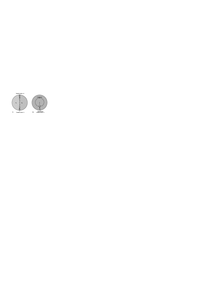
Figure 3: The manifold $M^{4}-M^{2}$ is covered by two charts $U_{+}$ and $U_{-}$. They overlap in two disconnected regions as shown in i). However, the transition function can be chosen to be trivial in one of the regions. The other region can be shrunk to an effectively three dimensional surface across which $A$ becomes discontinuous, as shown in ii).

Thus, with this choice of atlas, the connection is continuous as one goes around the defect except at $\Sigma$ where $\mathcal{A}_{+}$ and $\mathcal{A}_{-}$ are related by a gauge transformation: $\mathcal{A}_{+}|_{\Sigma}=\mathcal{A}_{-}^{h}|_{\Sigma}$,

$$\mathcal{A}^{h}:=h^{-1}\mathcal{A}h+h^{-1}dh\,.$$ (4)

In each chart the Characteristic form can be expressed as a total derivative so that $\int_{U_{\pm}}\langle\mathcal{F}\mathcal{F}\rangle=\int_{\partial U_{\pm}}CS(\mathcal{A}_{\pm})$, where $CS(\mathcal{A})$ is the Chern-Simons three form,

$$CS(\mathcal{A}):=\left\langle\mathcal{A}d\mathcal{A}+\frac{2}{3}\mathcal{A}^{3}\right\rangle\ .$$ (5)

The integral of (3) thus reduces to an integral over the contour depicted in figure 2,

$$\lim_{R\rightarrow 0}\int_{M^{4}-D^{2}\times M^{2}}\left\langle\mathcal{FF}\right\rangle = \int_{\Sigma_{+}^{3}}CS(\mathcal{A}_{-}^{h})+\int_{\Sigma_{-}^{3}}CS(\mathcal{A}_{-})$$ (6)

$$+\lim_{R\rightarrow 0}\left\{\int_{C^{+}\times M^{2}}CS(\mathcal{A}_{+})+\int_{C^{-}\times M^{2}}CS(\mathcal{A}_{-})\right\}$$

where $\partial U_{+}=\Sigma_{+}\bigcup(C^{+}\times M^{2})$ and $\partial U_{-}=\Sigma_{-}\bigcup(C^{-}\times M^{2})$ and $C^{\pm}$ are semi-circles such that $S_{R}^{1}=C^{+}\bigcup C^{-}$.

The first two integrals on the RHS of (6) correspond to the boundary of the charts on the intersecting region. Defining the orientation of $\Sigma$ by $\Sigma\equiv-\Sigma_{-}\equiv\Sigma_{+}$ (and dropping the subscript “$-$” from $\mathcal{A}_{-}$), they become

$$\int_{\Sigma_{+}^{3}}CS(\mathcal{A}^{h})+\int_{\Sigma_{-}^{3}}CS(\mathcal{A})=\int_{\Sigma}CS(\mathcal{A}^{h})-CS(\mathcal{A})\,.$$ (7)

Now let us turn to the last two terms in (6). These two integrals arise as further boundary terms along the $\mathbf{S}^{1}.$ The limit $R\rightarrow 0$ for these integrals seems to be, from a strict mathematical point of view, somewhat ambiguous. Let us introduce a regularisation process which will ensure that the integral on the RHS of (3) is invariant under gauge transformations $\mathcal{A}\rightarrow\mathcal{A}^{g}$, for any $g(x)$ that is single valued in the limit that $S_{R}^{1}$ shrinks to a point. We demand this because the integrand $\langle\mathcal{F}\mathcal{F}\rangle$ is gauge invariant and so the LHS should be invariant under any such gauge transformation. This will be achieved if

$$\int\limits_{C^{+}\times M^{2}}CS(\mathcal{A}_{+})+\int\limits_{C^{-}\times M^{2}}CS(\mathcal{A}_{-})\ \rightarrow\ \int\limits_{M^{2}}\langle\mathcal{A}\mathcal{A}^{h}\rangle\,.$$ (8)

As mentioned, the justification is ultimately the gauge invariance of the final result. However, it is possible to obtain equation (8) by an adequate regularization, which is given in the appendix.

Finally, setting that in the limit $\partial\Sigma=M^{2},$ and using the identity $CS(\mathcal{A}^{h})\equiv CS(\mathcal{A})-\frac{1}{3}\left\langle\left(h^{-1}dh\right)^{3}\right\rangle+d\left\langle h^{-1}\mathcal{A}dh\right\rangle$, allows writing (6) in a manifestly two-dimensional form as

$$\int_{M^{4}-M^{2}}\left\langle\mathcal{FF}\right\rangle=-\int_{\Sigma}\frac{1}{3}\left\langle\left(h^{-1}dh\right)^{3}\right\rangle+\int_{M^{2}}\left\langle\left(\mathcal{A}-h^{-1}dh\right)\mathcal{A}^{h}\right\rangle.$$ (9)

The RHS of (9) is a gWZW term, a two-dimensional action which has the desired property of invariance under the local transformations,

$$h\rightarrow g^{-1}hg,\qquad\mathcal{A}\rightarrow g^{-1}\mathcal{A}g+g^{-1}dg,$$ (10)

that defines a theory on the topological defect, $M^{2}$. The field equations, obtained by Euler-Lagrange variation with respect to $\mathcal{A}$ and $h$, are also invariant under the above gauge transformations.

It has been recognized that CS theory on a Riemann surface times $S^{1}$ is equivalent to a WZW model [22]. The equality (9) was conjectured to exist in [23]. We conclude that the two dimensional action to be considered is

$$S(h,\mathcal{A})=\kappa\int_{\Sigma}\frac{1}{3}\left\langle\left(h^{-1}dh\right)^{3}\right\rangle-\kappa\int_{M^{2}}\left\langle\left(\mathcal{A}-h^{-1}dh\right)\mathcal{A}^{h}\right\rangle,$$ (11)

The construction presented here generated a well known structure in two dimensions starting from a four-dimensional topological invariant: the gWZW terms that are the minimal gauge invariant extension of $\left\langle\left(h^{-1}dh\right)^{3}\right\rangle$. When a kinetic term for the Goldstone fields is added, a good part of two dimensional physics can be retrieved from this non-linear sigma model language: the description of the super-string [24]; the characterization of exact string backgrounds [25]; and the non-abelian bosonization phenomena [26], to name a few. The particular action described above, the G/G model, is special in that, even when the kinetic term is added, it defines a topological theory [27]. Thus, the $G/G$ model, both with and without kinetic term, define very closely related theories, as was discussed in Ref. [28]. In our construction, a kinetic term does not arise.

This construction has produced a well defined action with all relative coefficients fixed. The procedure can also be extended to build gravitational actions in $2n-2$ dimensions beginning from the Euler density in $2n$ dimensions.

2.2 The four-dimensional case

Applying the previous procedure to the six dimensional Euler density (2) yields

$$S(h,\mathcal{A})=\frac{\kappa}{48\pi^{3}}\int_{\Sigma}CS(\mathcal{A})-CS(\mathcal{A}^{h})-\frac{\kappa}{48\pi^{3}}\int_{M^{4}}B\left(\mathcal{A},\mathcal{A}^{h}\right),$$ (12)

where $CS(\mathcal{A})$ is now the CS five-form,

$$CS(\mathcal{A}):=\left\langle\mathcal{A}d\mathcal{A}d\mathcal{A}+\frac{3}{2}\mathcal{A}^{3}d\mathcal{A}+\frac{3}{5}\mathcal{A}^{5}\right\rangle,\;h=e^{\phi}=\exp(\frac{1}{2}J_{AB}\phi^{AB}),$$ (13)

and

$$B(\mathcal{A},\mathcal{A}^{h}):=\left\langle\mathcal{AA}^{h}\left(\mathcal{F}+\mathcal{F}^{h}-\frac{1}{2}\mathcal{A}^{2}-\frac{1}{2}\left(\mathcal{A}^{h}\right)^{2}+\frac{1}{2}\mathcal{AA}^{h}\right)\right\rangle.$$ (14)

Replacing the identity,

$$CS(\mathcal{A}) \equiv CS(\mathcal{A}^{h})+d\left\langle\left(h^{-1}dh\right)\left(\mathcal{A}^{h}\mathcal{F}^{h}-\frac{1}{2}\left(\mathcal{A}^{h}\right)^{3}\right)\right\rangle-\frac{1}{10}\left\langle\left(h^{-1}dh\right)^{5}\right\rangle$$ (15)

$$-d\frac{1}{2}\left\langle\left(h^{-1}dh\right)^{2}\mathcal{F}^{h}-\left(h^{-1}dh\right)\mathcal{A}^{h}\left(h^{-1}dh\right)\mathcal{A}^{h}\right\rangle$$

$$-d\frac{1}{2}\left\langle\left(h^{-1}dh\right)^{3}\mathcal{A}^{h}\right\rangle$$

back in (12) the action takes the form:

$$S(h,A) = -\kappa\int_{\Sigma}\frac{1}{480\pi^{3}}\left\langle\left(h^{-1}dh\right)\left(h^{-1}dh\right)^{2}\left(h^{-1}dh\right)^{2}\right\rangle$$ (16)

$$+\frac{\kappa}{48\pi^{3}}\int_{M^{4}}\left\langle\left(dhh^{-1}\right)\mathcal{A}\left(d\mathcal{A}+\frac{1}{2}\mathcal{A}^{2}\right)\right\rangle$$

$$-\frac{\kappa}{96\pi^{3}}\int_{M^{4}}\left\langle\left(dhh^{-1}\right)\mathcal{A}\left(\left(dhh^{-1}\right)^{2}+\mathcal{A}\left(dhh^{-1}\right)\right)\right\rangle$$

$$-\frac{\kappa}{48\pi^{3}}\int_{M^{4}}\left\langle\mathcal{AA}^{h}\left(\mathcal{F}+\mathcal{F}^{h}-\frac{1}{2}\mathcal{A}^{2}-\frac{1}{2}\left(\mathcal{A}^{h}\right)^{2}+\frac{1}{4}[\mathcal{A},\mathcal{A}^{h}]\right)\right\rangle$$

It must be stressed that the right normalization of the Wess-Zumino term was obtained from the normalized Euler characteristic (2) as a by-product of the construction, without a need for adjusting the parameters in the action (16). The normalized Wess-Zumino term for a group with $\pi_{5}(G)=\mathbb{Z}$ satisfies [29].

$$\int_{S^{5}}\frac{1}{480\pi^{3}}\left\langle\left(h^{-1}dh\right)^{5}\right\rangle=n\in\mathbb{Z},$$ (17)

where $n$ is the homotopy class to which the map $h:S^{5}\rightarrow G$ belongs.

Actions of the type (16) are widely used in particle physics to describe the infrared behavior of QCD [30, 31]. The gauged version was introduced originally by Witten in ref [14], where the motivation was to find a gauge invariant extension of the global $G\times G$ symmetry present in the five-dimensional closed form $\left\langle\left(h^{-1}dh\right)^{5}\right\rangle$. This problem is far from trivial, since the naive gauge extension of this term obtained by replacing the exterior derivative by a covariant derivative doesn’t work: if this is done, the 5-form is no longer closed and the field equations have support on the five-dimensional manifold $\Sigma$. Although far from obvious, the same gWZW structures that arise in the description of QCD may also be used to describe GR. While in QCD the gWZW term describes the interactions of the infrared sector of the theory, here it might correspond to an ultraviolet extension of GR.

The action (16) was proposed as a gravitational model in [18] where, in order to obtain Einstein’s field equations, a field was fixed in the action. That is a rather unsatisfactory situation since this is a condition imposed on a theory by an a posteriori expected result. In the next section we shall see that Einstein’s field equations arise from the action (16) without fixing fields in the action, but considering instead an ansatz that relies on the topological defect interpretation of the action.

The field equations associated with the variation with respect to $h$ are

$$\int_{M^{4}}\Big{\langle}h^{-1}\delta h\Big{\{}\!\left(\mathcal{F}^{h}\right)^{2}+\mathcal{F}^{2}+{}\!\mathcal{F}^{h}\mathcal{F}-\frac{3}{4}[{}\!\mathcal{A}^{h}-\mathcal{A},{}\mathcal{A}^{h}-\mathcal{A}]\ ({}\!\mathcal{F}^{h}+\mathcal{F})$$

$$+\frac{1}{8}[{}\!\mathcal{A}^{h}-\mathcal{A},{}\!\mathcal{A}^{h}-\mathcal{A}]^{2}+\frac{1}{2}({}\!\mathcal{A}^{h}-\mathcal{A})[{}\!\mathcal{F}^{h}+\mathcal{F},{}\!\mathcal{A}^{h}-\mathcal{A}])\Big{\}}\Big{\rangle}=0,$$ (18)

while those associated with the connection $\mathcal{A}$ are

$$0 = \int_{M^{4}}\Big{\langle}\delta\mathcal{A}\left(({}\!\mathcal{A}^{h}-\mathcal{A})\left({}\!\mathcal{F}^{h}+2\mathcal{F}-\frac{1}{4}[{}\!\mathcal{A}^{h}-\mathcal{A},{}\!\mathcal{A}^{h}-\mathcal{A}]\right)\right)\Big{\rangle}$$ (19)

$$-(h\leftrightarrow h^{-1}).$$

If one wishes to describe a four-dimensional world with Lorentzian signature, the gauge group to be chosen can only be $SO(5,1)$, $SO(4,2)$ or $SO(3,3)$. The discussion will be restricted from now to the $SO(4,2)$ group, as it is particularly interesting, allowing for the quantization of the coefficient $\kappa$ in front of the action [32]. In the next section we make contact between the action presented above and the Einstein equations.

3 The Einstein dynamical sector

The topological action (16) gives rise to first order field equations, is invariant by construction under coordinate transformations, and is also invariant under the local transformations,

$$h\rightarrow g^{-1}hg,\;\;\mathcal{A}\rightarrow g^{-1}(\mathcal{A}+d)g.$$ (20)

The theory contains 30 fields, the 15 components of $h\in SO(4,2)$, and 15 fields in the connection $\mathcal{A}=\frac{1}{2}\mathcal{A}^{AB}J_{AB}$. The introduction of a four-dimensional topological defect in the six-dimensional manifold splits the generators $J_{AB}$ into those that leave invariant the tangent space of $M^{4}$, $J_{ab},J_{45}$, and those that move it into the $4$ and $5$ directions, $J_{a4},J_{a5}$, where $a,b=0,...,3$ are Lorentz indices. It is therefore natural to separate the generators into their irreducible Lorentz covariant parts $(J_{ab},J_{a5},J_{a4},J_{45})$. Correspondingly, the connection is written as

$$\mathcal{A}=\frac{1}{2}\omega^{ab}J_{ab}+c^{a}J_{a5}+b^{a}J_{a4}+\Phi J_{45}\;,$$ (21)

and the curvature reads

$$\mathcal{F} = \frac{1}{2}(R^{ab}+c^{a}c^{b}-b^{a}b^{b})J_{ab}+[Db^{a}+c^{a}\Phi]J_{a4}+[Dc^{a}+b^{a}\Phi]J_{a5}$$ (22)

$$+[d\Phi-b_{a}c^{a}]J_{45}.$$

Here $(J_{ab},J_{a5})$ and $(J_{ab},J_{a4})$ span the $so(3,2)$ and $so(4,1)$ subalgebras of $SO(4,2)$, respectively; $R^{ab}=d\omega^{ab}+\omega_{\;c}^{a}\omega^{cb}$ is the Lorentz curvature two-form and $Dc^{a}=dc^{a}+\omega_{\;b}^{a}c^{b}$. Note that the vielbein should be identified as a vector under local Lorentz rotations. At this point there is no strong reason to choose either $b$ or $c$, or any linear combination thereof, as the vielbein.

In order to write down the field equations it is necessary to give a parametrization of the group element. A convenient one can be constructed as follows: take the Cartan decomposition $\mathfrak{g}=\mathfrak{p}\oplus\mathfrak{q}$, where $\mathfrak{q}$ is the maximal compact subalgebra of $\mathfrak{g}$, $\mathfrak{p}=\mathfrak{g}-\mathfrak{q}$ and the semidirect sum stands for $\left[\mathfrak{p},\mathfrak{p}\right]\subset\mathfrak{q}$, $\left[\mathfrak{q},\mathfrak{p}\right]\subset\mathfrak{p}$, $\left[\mathfrak{q},\mathfrak{q}\right]\subset\mathfrak{q}$, the $so(4)$ indexes are denoted by $\overline{a}=\left\{1,2,3,4\right\}$, so that $\mathfrak{q}$ is spanned by $\left\{J_{\overline{ab}},J_{05}\right\}$ and $\mathfrak{p}$ by $\left\{J_{5\overline{a}},J_{0\overline{a}}\right\}$, now due to this decomposition any group element $g\in G$ can be written as $g=pq$, where $q$ is in the maximal compact proper subgroup of $G$, $q\in Q=SO(4)\times SO(2)\subset G$, and $p$ is in its complement, $p\in P\subset G$. Any group element of $P$ belongs to an orbit of the adjoint action of $Q$ on the exponential of a Cartan subalgebra $\mathfrak{a}\subset\mathfrak{p}$ (see for instance, [33]). Thus we have the decomposition of $G=QAQ$. Applying this decomposition to $SU(2)$, for instance, gives the standard parametrization in terms of the Euler angles and can be used in general to decompose a given group in one parameter subgroups simplifying, in this way, the computations. In our case, is enough to implement a partial decomposition and the result is (See the appendix for more details)

$$h=h_{o}e^{\beta J_{12}}e^{\lambda J_{24}}e^{\delta J_{23}}e^{\left(z^{\bar{a}}J_{0\bar{a}}+\rho J_{52}\right)}e^{\alpha J_{05}}e^{\zeta^{\overline{ab}}J_{\overline{ab}}}$$ (23)

where $h_{o}$ is a constant group element whose effect corresponds to a change in the origin of the parametrization. In our case, $h_{o}$ corresponds to the nontrivial identification that is made in the six-dimensional manifold that gives rise to the defect. The presence of $h_{o}$ reflects the fact that the defect generates a non-dynamical transition function of the six dimensional bundle. The fields $\beta,\lambda,\delta,z,\rho,\alpha,\zeta$, on the other hand, are fluctuations around $h_{o}$. Since the directions transverse to the tangent space of the topological defect are $4$ and $5$, the “vacuum” of the theory can be identified with the constant transition function $h_{o}=e^{\theta_{o}J_{45}}$.

On shell we fix $\lambda=\delta=\alpha=\beta=z=\rho=\zeta=0$. This anzats simplifies the field equations enough to write them down by components. From (19) it is straightforward to obtain (see appendix)

$$\delta\Phi : 0=0,$$ (24)

$$\delta c^{a} : \varepsilon_{abcd}c^{b}\left(3R^{cd}+\left(2+\cosh\theta_{0}\right)\left(c^{c}c^{d}-b^{c}b^{d}\right)\right)\sinh\theta_{0}=0,$$ (25)

$$\delta b^{a} : \varepsilon_{abcd}b^{b}\left(3R^{cd}+\left(2+\cosh\theta_{0}\right)\left(c^{c}c^{d}-b^{c}b^{d}\right)\right)\sinh\theta_{0}=0,$$ (26)

$$\delta\omega^{ab} : 3\varepsilon_{abcd}\left(b^{c}Db^{d}-c^{c}Dc^{d}\right)\sinh\theta_{0}=0,$$ (27)

At this point it is clear that the choices of $b$ or $c$ as the vielbein correspond to having a positive or negative cosmological constant, respectively. In order to see that the Einstein equation are contained in this system, it is sufficient to set $b=0$, keeping $c$ as the vielbein, and requiring that $\theta_{0}\neq 0$. This further reduces the previous set of equations to

$$\varepsilon_{abcd}c^{b}\left(R^{cd}+\mu c^{c}c^{d}\right) = 0,$$ (28)

$$\varepsilon_{abcd}c^{c}Dc^{d} = 0,$$ (29)

where $\mu=\frac{2+\cosh\theta_{0}}{3}$. Furthermore, the field equations obtained varying with respect to $h$, (18), are identically satisfied by $\Phi=0$. This can be seen by substituting the ansatz (23) into the field variations (18). The components $(h^{-1}\delta h)^{ab}$, $(h^{-1}\delta h)^{a4}$ and $(h^{-1}\delta h)^{a5}$ give field equations proportional to the torsion $T^{c}=Dc^{b}$, and therefore are identically satisfied by virtue of (29). The last component gives

$$(h^{-1}\delta h)^{45}\Big{(}R^{ab}+\mu c^{a}c^{b}\Big{)}\Big{(}R^{cd}+\mu c^{c}c^{d}\Big{)}\varepsilon_{abcd}=0\,.$$ (30)

Although this equation might seem to give a further restriction on the geometry, that is not the case because $\left.(h^{-1}\delta h)^{45}\right|_{h=h_{0}}=0$, as can be easily verified for (23). It must be stressed, however, that this is not a property of the form chosen of the parametrization (23); any other parametrization obtained by gauge transformation compatible with the presence of the defect would yield a physically equivalent set of equations.

As in the three-dimensional case, when GR is regarded as a gauge theory [14], contact with the metric phase of the theory makes it necessary to require the vielbein to be invertible, $c_{\mu}^{\;a}c_{\;a}^{\nu}=\delta_{\mu}^{\nu}$, $c_{\mu}^{\;a}c_{\;b}^{\mu}=\delta_{b}^{a}$. The introduction of a parameter with dimensions of length, $l$, is also necessary in order to make $\bar{c}_{\mu}^{a}=l^{-1}c_{\mu}^{a}$ dimensionless. These two conditions allow to regard $\bar{c}_{\mu}^{a}$ as an isomorphism between the coordinate tangent space and the non-coordinate one, such that the relation $g_{\mu\nu}=\bar{c}_{\mu}^{\;a}\bar{c}_{\nu}^{\;b}\eta_{ab}$ makes sense. Using this, equation (28) and the zero-torsion condition (29), reproduce the Einstein field equations for the metric, $g_{\mu\nu}$,

$$R_{\mu\nu}-\frac{1}{2}g_{\mu\nu}R-\Lambda g_{\mu\nu}=0,$$ (31)

where $R_{\mu\nu}$ is the metric-compatible Ricci tensor and $\Lambda=l^{-2}\left(2+\cosh\theta_{0}\right)$ is the cosmological constant.

However, the semiclasical description of gravitational solutions is also related to the form of the action. In order to describe Einstein’s gravity as a minisuperspace of this gauged WZW theory, it is also necessary to recover the Einstein Hilbert action. This can be done by replacing the ansatz

$$\mathcal{A}=\frac{1}{2}\omega^{ab}J_{ab}+c^{a}J_{a5}\;,\;\;h=e^{\theta_{0}J_{45}}$$ (32)

in the action (16), reducing it to

$$\frac{\kappa\sinh\theta_{0}}{32\pi^{3}}\int_{M^{4}}\varepsilon_{abcd}c^{a}c^{b}\left(R^{cd}+\frac{1}{2}\mu c^{c}c^{d}\right)\,.$$ (33)

This is indeed the Einstein-Hilbert action that gives GR with the same cosmological constant that one obtains by putting the ansatz into the full set of field equations, thereby justifying the use of a mini-superspace action.

4 Quantization of $\kappa$ and Euclidean continuation

The conditions under which the constant $\kappa$ takes integer values are well known [20, 32]. Consider a non-linear sigma model defined by the map

$$h:S^{4}\longrightarrow G.$$

If $S^{4}$ is viewed as the boundary of some compact manifold $D^{5}$, one can consider the extension of the map $h$ to the interior ($\partial D^{5}=S^{4}$),

$$h:D^{5}\longrightarrow G.$$

However, $S^{4}$ can be the boundary of many different interiors. Imposing independence of the path integral under a change of given interior $D^{5}$ by another, $\overline{D}^{5}$ requires

$$S=\kappa\int_{D^{5}}\frac{1}{480\pi^{3}}\left\langle\left(h^{-1}dh\right)^{5}\right\rangle=\kappa\int_{\overline{D}^{5}}\frac{1}{480\pi^{3}}\left\langle\left(h^{-1}dh\right)^{5}\right\rangle+2\pi m\hbar.$$ (34)

Therefore, the integral over the manifold, $M^{5}=D^{5}\bigcup(-\overline{D}^{5})$, where the minus denotes the correct orientation, is found to be

$$\kappa\int_{M^{5}}\frac{1}{480\pi^{3}}\left\langle\left(h^{-1}dh\right)^{5}\right\rangle=2\pi m\hbar,$$ (35)

where the manifold $M^{5}$ is compact and without boundary. Now if $\pi_{5}(G)=\mathbb{Z}$ then, from (17), one concludes that $\kappa n=2\pi m\hslash$ and, as this must be true for all $n$, one concludes that $\kappa$ itself must be quantized,

$$\kappa=2\pi n\hslash\ .$$ (36)

This quantization holds for compact groups $G$, but the groups we are considering here are not necessarily compact. However, there are complex extensions of them that are compact. The argument presented here still holds if one allows for analytic continuations of the theory, defined by the map of the connection

$$\mathcal{A}^{\bar{a}\bar{b}} \rightarrow \overline{\mathcal{A}}^{\bar{a}\bar{b}}=\mathcal{A}^{\bar{a}\bar{b}},\;\mathcal{A}^{\bar{a}0}\rightarrow\overline{\mathcal{A}}^{\bar{a}0}=i\overline{\mathcal{A}}^{\bar{a}0}$$

$$\mathcal{A}^{\bar{a}5} \rightarrow \overline{\mathcal{A}}^{\bar{a}5}=i\mathcal{A}^{\bar{a}5},\;\mathcal{A}^{05}\rightarrow\overline{\mathcal{A}}^{05}=-\overline{\mathcal{A}}^{05}.$$

The same map must be applied to the Goldstone fields. The resulting action is invariant under $SO(6)$, as can be seen by the equivalent map of the generators

$$J_{\bar{a}0} \rightarrow \bar{J}_{\bar{a}0}=iJ_{\bar{a}0},\;\;J_{\bar{a}5}\rightarrow\bar{J}_{\bar{a}5}=iJ_{\bar{a}5}$$

$$J_{05} \rightarrow \bar{J}_{05}=-J_{05},\;\;J_{\bar{a}\bar{b}}\rightarrow\bar{J}_{\bar{a}\bar{b}}=J_{\bar{a}\bar{b}}$$ (37)

where the new indexes $\bar{a},\bar{b}$ cover the range $1,...,4$, and the new metric is Euclidean, $\delta_{\bar{a}\bar{b}}=\left(+,+,+,+\right)$. Under these changes, the invariant tensor $\langle J_{AB}J_{CD}J_{EF}\rangle$ reverses sign and so does the action (16), $S\rightarrow-S$.

On the other hand, the Euclidean continuations of the groups $SO(5,1)$ and $SO(3,3)$ instead, give rise to additional imaginary factors in the action,

$$SO(5,1)\rightarrow SO(6)\quad \Rightarrow\quad e^{\frac{i}{\hslash}\kappa S}\rightarrow e^{-\frac{\kappa}{\hslash}S}\,,$$

$$SO(3,3)\rightarrow SO(6)\quad \Rightarrow\quad e^{\frac{i}{\hslash}\kappa S}\rightarrow e^{\frac{\kappa}{\hslash}S}.$$

We see that the group $SO(4,2)$ has the particular property that since its Euclidean continuation changes the action by a sign and not by an imaginary factor, i.e.

$$SO(4,2)\rightarrow SO(6)\quad\Rightarrow\quad e^{\frac{i}{\hslash}\kappa S}\rightarrow e^{-\frac{i}{\hslash}\kappa S}\,,$$ (38)

it allows for the existence of the phase freedom (36). Conversely, requiring the coefficient in front of the action to be quantized, singles out the gauge group to be $SO(4,2)$.

5 Discussion and Outlook

Here, a six-dimensional gauge theory that gives rise to four-dimensional GR has been proposed. The starting action (16) is metric-independent, and all the fields have a geometrical interpretation. Besides the usual connection $\mathcal{A}$, the transition function $h$ around the four-dimensional defect embedded in six dimensions is also present. These two objects ($\mathcal{A},h$) are completely defined once a principal bundle is given over $M^{6}$.

The theory generalizes GR since it contains a dynamical sector in which Einstein’s equations hold, presumably reproducing all the experimental tests that are compatible with GR. The Einstein-Hilbert Lagrangian is obtained as the topological dimensional reduction of the six-dimensional Euler density by the presence of the four-dimensional topological defect. In this way, a theory that contains other fields besides GR is obtained, something that could be welcome in the current state of affairs, where several models have been advanced to explain the dynamics of the galaxies, inflation, or dark matter in the Universe, and other phenomena that cannot be explained using only GR and standard matter fields.

The purely gravitational sector studied here has classically zero torsion, but the full theory naturally includes torsion. The presence of propagating torsion in a background configuration changes many of the known results in GR, including those about the generic existence of singularities in spacetime [34].

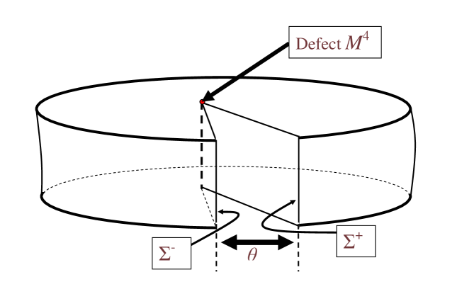
Figure 4: The physical interpretation of the transition function $h=\exp(\theta J_{45})$ as a defect caused by removing a wedge from the six-dimensional manifold. It should be remembered that the defect is parameterized by a hyperbolic angle, so this figure actually represents the Euclideanized version discussed in section 4.

The transition functions represent topological information (fig.4) of the six-dimensional action and become dynamical in the four-dimensional theory. Their presence could be interpreted as the deconfining phase of the higher dimensional, topological theory and they could even be relevant to the description of our Universe.

The emergence of the space-time causal structure in the theory defined by (16) arises only after a vielbein is chosen from amongst all the invertible linear combinations of the $b$ and $c$.

Because of the non-trivial choice $h=\exp(\theta_{0}J_{45})$, the gauge invariance of the theory is on shell reduced to SO(3,1)$\times$SO(1,1). The choice $b^{a}=0$, $c^{a}\neq 0$ further breaks the SO(1,1) symmetry generated by $J_{45}$, leaving the Lorentz group SO(3,1) as the remanent gauge symmetry. The invertibility of what is chosen as a vielbein is not affected by this remanent gauge symmetry: the vielbein $c^{a}$ transforms as a vector under local Lorentz rotations.

The obtention of a gravitation theory that is metric independent; in which GR could be seen as a broken phase of a topological field theory has been a long sought goal [35]. The construction presented here is a step in this direction.

Acknowledgments
The authors wish to thank Eloy Ayón-Beato, Glenn Barnich, Fabrizio Cánfora, Steven Carlip, Frank Ferrari, Joaquim Gomis, Marc Henneaux, Matias Leoni, Rafael Sorkin and Ricardo Troncoso for enlightening discussions. Special thanks are given to Gastón Giribet for his careful reading of the manuscript, helping us to clarify several points. A.A. wishes to thank the warm hospitality and the stimulating questions received at the General Relativity workshop, Universidad de Buenos Aires (UBA) and the Instituto de Astronomía y Física del Espacio (IAFE), where this work was presented; the support of MECESUP UCO 0209 and CONICYT grants is also acknowledged. This work has been supported in part by FONDECYT grants Nos. 1040921, 1060831, 1061291, 3060016, and by an institutional grant to the Centro de Estudios Científicos (CECS) from the Millennium Science Initiative. Institutional support to CECS from Empresas CMPC is gratefully acknowledged.

Appendix A Appendix

The regularisation process:

Here we give an argument to justify equation (8). Let $t$ be a coordinate on $S_{R}^{1}$ (anticlockwise) such that the charts in $S^{1}$ are given by the range of coordinates $C^{-}=(0,t_{\Sigma})$ and $C^{+}=(t_{\Sigma},1)$ where $t$ is periodically identified $t\equiv t+1$. Let us introduce a family of functions $p_{n}(t)$ which, for each $n$, give a partition of unity on $S_{R}^{1}$ and which converge to the Heaviside step function $\lim_{n\rightarrow\infty}p_{n}(t)=\theta(t-t_{\Sigma})$. The last two integrals in (6) can be expressed as:

$$\int\limits_{C^{+}\times M^{2}}CS(\mathcal{A}_{+})+\int\limits_{C^{-}\times M^{2}}CS(\mathcal{A}_{-})=\int\limits_{S_{R}^{1}\times M^{2}}\left[1-p_{n}(t)\right]CS(\mathcal{A}_{+})+p_{n}(t)\,CS(\mathcal{A}_{-})\,.$$ (A.1)

Note that $\mathcal{A}_{\pm}$ in regions $C^{\pm}$ define a non-trivial bundle on $S_{R}^{1}$ that can not be extended to the interior of $D_{R}^{2}$. Let us define a new connection $\mathcal{A}_{n}:=\mathcal{A}_{+}\left[1-p_{n}(t)\right]+\mathcal{A}_{-}p_{n}(t)$ on $S_{R}^{1}$ which can be extended into the interior since it is a single connection (continuous for finite $n$, distributional for $n\rightarrow\infty$). Using the property that $\lim_{n\rightarrow\infty}p_{n}^{2}(t)=\lim_{n\rightarrow\infty}p_{n}^{3}(t)=\theta(t-t_{\Sigma})$, it is possible to further show that:

$$\lim_{n\rightarrow\infty}\int\limits_{S_{R}^{1}\times M^{2}}\left(1-p_{n}\right)CS(\mathcal{A}_{+})+p_{n}\ CS(\mathcal{A}_{-})$$

$$\qquad=\lim_{n\rightarrow\infty}\left[\int\limits_{S_{R}^{1}\times M^{2}}CS(\mathcal{A}_{n})-\int\limits_{S_{R}^{1}\times M^{2}}\dot{p}_{n}\langle{\mathcal{A}}_{+}\mathcal{A}_{-}\rangle\right]$$

$$\qquad=\lim_{n\rightarrow\infty}\int\limits_{S_{R}^{1}\times M^{2}}CS(\mathcal{A}_{n})+\int\limits_{M^{2}}\left.\langle\mathcal{AA}^{h}\rangle\right|_{t=t_{\Sigma}}\,.$$ (A.2)

So for large $n$ we have

$$\int\limits_{C^{+}\times M^{2}}CS(\mathcal{A}^{h})+\int\limits_{C^{-}\times M^{2}}CS(\mathcal{A})\approx-\int\limits_{D_{R}^{2}\times M^{2}}\langle\mathcal{F}_{n}\mathcal{F}_{n}\rangle+\int\limits_{M^{2}}\langle\mathcal{AA}^{h}\rangle\,.$$ (A.3)

Now, being the manifold $D_{R}^{2}\times M^{2}$ regular and the curvature, $\mathcal{F}_{n}$, globally defined, it is reasonable to suppose that the integral of $\langle\mathcal{F}_{n}\mathcal{F}_{n}\rangle$ vanishes for $R\rightarrow 0$, in which case we recover equation (8).

The following convention for the $SO(4,2)$ algebra was used:

$$\left[J_{AB},J_{CD}\right]=-J_{AC}\eta_{BD}+J_{BC}\eta_{AD}-J_{BD}\eta_{AC}+J_{AD}\eta_{BC},$$ (A.4)

$$A=0,...,5\ ,\quad\eta_{AB}=\left(-,+,+,+,+,-\right).$$ (A.5)

Some notation: Einstein’s Equation as a three-form.

We have encountered the Einstein equation in differential form language. To make contact with a more familiar tensorial form of the field equation, one must require that the vielbein is not degenerate. The field equation is:

$$\varepsilon_{abcd}\ e^{b}\wedge R^{cd}\ =\ \frac{1}{2}\varepsilon_{abcd}\ R_{\ \ ef}^{cd}\ e^{b}\wedge e^{e}\wedge e^{f}=0\,.$$ (A.6)

Then the trick is simply to dualise this three form:

$$\varepsilon_{abcd}\ R_{\ \ ef}^{cd}\ \varepsilon^{befg}=0$$

Now one makes use of the identity $\varepsilon_{abcd}\ \varepsilon^{befg}=\delta_{acd}^{efg}$, where the $\delta$ is the totally antisymmetrised Kronecker delta. One obtains

$$R_{\ \nu}^{\mu}-\frac{1}{2}\delta_{\ \nu}^{\mu}\ R=0,$$

To avoid notational confusion ($R_{\ \nu}^{\mu}$ is the Ricci tensor, not to be confused with $R^{ab}$ which is the curvature two-form) the indices have been converted to coordinate basis indices using the vielbein $e_{\mu}^{a}$ and its inverse. The familiar tensorial form of Einstein’s field equation is thus recovered.

Some useful formulas

Given $h=e^{\theta J_{45}}$, it is possible to compute:

$$\mathcal{A}^{h} = \frac{1}{2}\omega_{ab}J^{ab}+J_{a4}\left(b^{a}\cosh\theta+c^{a}\sinh\theta\right)+J_{a5}\left(c^{a}\cosh\theta+b^{a}\sinh\theta\right)$$ (A.7)

$$+\left(\Phi+d\theta\right)J_{45}$$

$$\mathcal{F}^{h} = \frac{1}{2}\left(R^{ab}+c^{a}c^{b}-b^{a}b^{b}\right)J_{ab}+J_{a4}\left[\left(Db^{a}+c^{a}\Phi\right)\cosh\theta+\sinh\theta\left(Dc^{a}+b^{a}\Phi\right)\right]$$

$$+J_{a5}\left[\left(Dc^{a}+b^{a}\Phi\right)\cosh\theta+\sinh\theta\left(Db^{a}+c^{a}\Phi\right)\right]+\left(d\Phi-b^{a}c_{a}\right)J_{45}$$

$$\left[\mathcal{A}^{h}-\mathcal{A},\mathcal{A}^{h}-\mathcal{A}\right] =2\left(1-\cosh\theta\right)\left(c^{a}c^{b}-b^{a}b^{b}\right)J_{ab}$$

$$\quad+2\left(\left(\cosh\theta-1\right)c^{a}+\sinh\theta b^{a}\right)d\theta J_{a4}$$

$$\quad+2\left(\left(\cosh\theta-1\right)b^{a}+\sinh\theta c^{a}\right)d\theta J_{a5}$$

$$\quad+4\left(1-\cosh\theta\right)c^{a}b^{b}\eta_{ab}\,J_{45}$$ (A.8)

On the group parametrization

How the parametrization used in this paper arise from the Cartan discomposition,

$$h=h_{o}e^{x^{\bar{a}}J_{5\bar{a}}+y^{\bar{a}}J_{0\bar{a}}}k\$$ (A.9)

where $k$ is an arbitrary group element of the maximal compact subgroup of $SO(4,2)$, can be explicitly checked as follows: first note that

$$e^{\beta J_{12}}e^{\lambda J_{24}}e^{\delta J_{23}}\rho J_{52}e^{-\delta J_{23}}e^{-\lambda J_{24}}e^{-\beta J_{12}}=x^{\bar{a}}J_{5\bar{a}}$$ (A.10)

where

$$x^{1} = \rho\sin\beta\cos\delta\cos\lambda,\;$$

$$x^{2} = \rho\cos\beta\cos\delta\cos\lambda,\;$$

$$x^{3} = -\rho\sin\delta\;x^{4}=-\rho\cos\delta\sin\lambda.$$ (A.11)

It follows that

$$x^{\bar{a}}J_{5\bar{a}}+y^{\bar{a}}J_{0\bar{a}}=e^{\beta J_{12}}e^{\lambda J_{24}}e^{\delta J_{23}}\left(z^{\bar{a}}J_{0\bar{a}}+\rho J_{52}\right)e^{-\delta J_{23}}e^{-\lambda J_{24}}e^{-\beta J_{12}}$$ (A.12)

where the redefinition in the coordinates

$$z^{1} = y^{1}\cos\beta-y^{2}\sin\beta$$

$$z^{2} = y^{1}\cos\lambda\sin\beta\cos\delta+y^{2}\cos\beta\cos\lambda\cos\delta-y^{3}\sin\delta-y^{4}\cos\delta\sin\lambda$$

$$z^{3} = y^{1}\sin\beta\cos\lambda\sin\delta+y^{2}\cos\beta\cos\lambda\sin\delta+y^{3}\cos\delta-y^{4}\sin\lambda\sin\delta$$

$$z^{4} = y^{1}\sin\beta\sin\lambda+y^{2}\cos\beta\sin\lambda+y^{4}\cos\lambda$$ (A.13)

was used. Finally the group element can be written as

$$h=h_{o}e^{\beta J_{12}}e^{\lambda J_{24}}e^{\delta J_{23}}e^{\left(z^{\bar{a}}J_{0\bar{a}}+\rho J_{52}\right)}k_{1}\$$ (A.14)

where $k_{1}=e^{-\delta J_{23}}e^{-\lambda J_{24}}e^{-\beta J_{12}}k$ is an arbitrary compact subgroup element.

References

- [1] D. Lovelock, J. Math. Phys. 12 (1971) 498.
- [2] B. Zumino, Phys. Rept. 137 (1986) 109.
- [3] B. Zwiebach, Phys. Lett. B 156 (1985) 315.
- [4] F. Mueller-Hoissen, Class. Quant. Grav. 3 (1986) 665.
- [5] G. Giribet, J. Oliva and R. Troncoso, JHEP 0605 (2006) 007 [arXiv:hep-th/0603177].
- [6] J. Edelestein, M. Hassaine, R. Troncoso, and J. Zanelli, Phys. Lett. B640 (2006) 278 [arXiv: hep-th/0605174].
- [7] J. Gomis and S. Weinberg, Nucl. Phys. B 469 (1996) 473 [arXiv:hep-th/9510087].
- [8] G. ’t Hooft and M. J. G. Veltman, Annales Poincare Phys. Theor. A 20 (1974) 69.
- [9] M. T. Grisaru, P. van Nieuwenhuizen and J. A. M. Vermaseren, Phys. Rev. Lett. 37 (1976) 1662.
- [10] M. H. Goroff and A. Sagnotti, Nucl. Phys. B 266 (1986) 709.
- [11] S. Deser and J. H. Kay, Phys. Lett. B 76 (1978) 400.
- [12] Z. Bern, Living Rev. Rel. 5 (2002) 5 [arXiv:gr-qc/0206071].
- [13] A. Achúcarro and P. K. Townsend, Phys. Lett. B 180 (1986) 89.
- [14] E. Witten, Nucl. Phys. B 311, 46 (1988).
- [15] S. Deser, J. G. McCarthy and Z. Yang, Phys. Lett. B 222 (1989) 61.
- [16] G. Bonelli and A. Boyarsky, Phys. Lett. B 490 (2000) 147 [arXiv:hep-th/0004058].
- [17] A. Boyarsky and B. Kulik, Phys. Lett. B 532 (2002) 357 [arXiv:hep-th/0202049].
- [18] A. Anabalón, S. Willison and J. Zanelli, Phys. Rev. D 75 (2007) 024009 [arXiv:hep-th/0610136].
- [19] M. Nakahara, “Geometry, Topology and Physics”, Institute of Physics; second edition, Bristol (2003).
- [20] E. Witten, Nucl. Phys. B 223, 422 (1983).
- [21] J. A. de Azcárraga and J. M. Izquierdo, “Lie groups, Lie algebras, cohomology and some applications in physics” Cambridge University Press; New Ed edition (September 13, 1998)
- [22] G. W. Moore and N. Seiberg,Phys. Lett. B 220 (1989) 422.
- [23] J. C. Baez, Commun. Math. Phys. 193 (1998) 219 [arXiv:gr-qc/9702051].
- [24] M. Henneaux and L. Mezincescu, Phys. Lett. B 152 (1985) 340.
- [25] E. Witten, Phys. Rev. D 44 (1991) 314.
- [26] E. Witten, Commun. Math. Phys. 92, 455 (1984).
- [27] E. Witten, Commun. Math. Phys. 144, 189 (1992).
- [28] E. Witten, arXiv:hep-th/9312104.
- [29] R. Bott and R. Seeley, Commun. Math. Phys. 62 (1978) 235.
- [30] S. R. Coleman, J. Wess and B. Zumino, Phys. Rev. 177 (1969) 2239.
- [31] C. G. Callan, S. R. Coleman, J. Wess and B. Zumino, Phys. Rev. 177 (1969) 2247.
- [32] J. Zanelli, Phys. Rev. D 51 (1995) 490 [arXiv:hep-th/9406202].
- [33] R. Hermann 1966 “Lie Groups for physicists,” (New York: Bejamin)
-
[34]
Singularity theorems generically include as hypotheses
that the connection is metric compatible and torsion free [see S.W.Hawking
and G.F.R. Ellis, The Large Scale Structure of Spacetime, Cambridge
U.P. (1973)]. Although the first hypothesis is physically motivated, the
second is not, and eliminating it changes the form of the equation of
geodesic deviation: take a smooth 1-parameter system of geodesics described
by a smooth map from a strip into , where each
geodesic is given by setting , define the coordinates vectors and the acceleration relative as . With usual definition of torsion and curvature,
it follows that
The second term is normally ignored in the equation of geodesic deviation. Thus, the inclusion of torsion could change the bounds for the energy momentum tensor to cause singularities. - [35] E. Witten, Phys. Lett. B 206 (1988) 601.