A new variational perturbation method for double well oscillators

Abstract

We propose a variational perturbation method based on the observation that eigenvalues of each parity sector of both the anharmonic and double-well oscillators are approximately equi-distanced. The generalized deformed algebra satisfied by the invariant operators of the systems provides well defined Hilbert spaces to both of the oscillators. There appears a natural expansion parameter defined by the ratios of three distance scales of the trial wavefunctions. The energies of the ground state and the first order excited state, in the $0^{th}$ order variational approximation, are obtained with errors $<10^{-2}$% for vast range of the coupling strength for both oscillators. An iterative formula is presented which perturbatively generates higher order corrections from the lower order invariant operators and the first order correction is explicitly given.

I Introduction

There are two well known problems in studying the anharmonic and the double-well oscillators. The first is that a naive perturbation theory of anharmonic oscillator leads to a divergent perturbation series even for an infinitesimal value of the coupling strength due to the eventual dominance of the perturbative correction over the un-perturbed contribution for large amplitude of oscillation bender . To remedy this difficulty several generalized perturbation methods have been developed friedberg ; justin . There have been many recent developments which provide well defined perturbative iterative solutions for the eigenvalues and eigenfunctions mei ; weinstein ; friedberg ; mahapatra ; turbiner . An interesting differential equation method, in parallel with Mathieu equation, was presented by Liang and Müller-Kirsten liang . A through analysis for this asymptotic perturbation and large order behaviors was given in Ref. muller .

Another difficulty is that a double-well oscillator has completely different algebraic structure and ground state wavefunction from those of anharmonic oscillator. Therefore, most perturbative approaches treat the two oscillators separately weinstein ; friedberg . The transition from a single-well system to a double-well system of a time-dependent oscillator was calculated through a nonperturbative method such as the WKB approximation bhattacharya ; gildener or by accommodating contributions from many excited states in addition to the ground states of symmetric oscillator banerjee . Even though these methods provide good approximations to the ground state and excited state energies, its generalization to field theory of infinite degrees of freedom or to time-dependent systems with symmetry-breaking-like phenomena encounters difficulties. Therefore, it is important to establish a consistent approximation method that can treat both of the oscillators in the same way. This subject has not been extensively studied compared to the problem of divergent perturbation.

The purpose of the present paper is to present a possible resolution to the second problem using a variational perturbation method. We present a unified treatment of the anharmonic and the double-well oscillators in the point of view of a generalized deformed oscillator. This provides an algebraic method in which the two oscillators are dealt with on an equal footing. We also present a natural expansion parameter defined by the ratios of three length scales appearing in the trial wavefunction. Its numerical value is smaller than $1/2$ for all physical parameter range of the system for the double-Gaussian trial wavefunctions used in this paper. To do these, we solve the Liouville-von Neumann (LvN) equation perturbatively.

The generalized deformed oscillator bonatsos was developed in the approach of quantum group theory drinfeld ; chai . The algebra is generated by the operators $\{1,a,a^{\dagger},N\}$ and the structure function $\Phi(x)$, satisfying the relations

$$~{}[a,N] = a,~{}~{}[a^{\dagger},N]=-a^{\dagger},$$ (1)

$$a^{\dagger}a = \Phi(N)=[N],~{}~{}~{}aa^{\dagger}=\Phi(N+1)=[N+1],$$

where $N$ is the number operator and $\Phi(x)$ is a positive analytic function with the condition

$$\Phi(0)=0.$$

This ensures the vacuum state $|0\rangle$ to be defined as the eigenstate of $N$ with zero eigenvalue and satisfies

$$a|0\rangle=0.$$

It can be proved that the generalized deformed algebra provides a Hilbert space of eigenvectors $|0\rangle,~{}|1\rangle,~{}\cdots,|n\rangle,\cdots$ of the number operator $N$ with $\langle n|m\rangle=\delta_{mn}$. These eigenvectors are generated by the formula,

$$|n\rangle=\frac{1}{\sqrt{[n]!}}\left(\hat{a}^{\dagger}\right)^{n}|0\rangle,~{}~{}~{}[n]!=\prod_{k=1}^{n}[k]=\prod_{k=1}^{n}\Phi(k).$$

The operators $a^{\dagger}$ and $a$ are the creation and the annihilation operators of this deformed oscillator:

$$\hat{a}|n\rangle=\sqrt{[n]}|n-1\rangle,~{}~{}~{}\hat{a}^{\dagger}|n\rangle=\sqrt{[n+1]}|n+1\rangle.$$

The harmonic oscillator is obtained for $\Phi(n)=n$ and the $q-$deformed oscillator for $\displaystyle\Phi(n)=\frac{q^{n}-q^{-n}}{q-q^{-1}}$ with the Hamiltonian, $\displaystyle H=\frac{\hbar\omega}{2}(\hat{a}\hat{a}^{\dagger}+\hat{a}^{\dagger}\hat{a})$.

The Hamiltonian describing both the anharmonic oscillator and the double-well oscillator is given by

$$H=\frac{\hat{p}^{2}}{2}+\frac{\omega^{2}}{2}\hat{x}^{2}+\frac{\lambda}{4}\hat{x}^{4},$$ (2)

with $\omega^{2}$ being a positive (anharmonic) or a negative (double-well) real number. For $\lambda\rightarrow 0$ with $\omega^{2}>0$, the system becomes a harmonic oscillator (harmonic oscillator limit) and for $\omega^{2}<0$ with $\lambda\rightarrow 0_{+}$ the system describes a set of two separated wells of harmonic oscillators (infinitely separated double-well limit).

The LvN equation lewis ,

$$0\equiv i\hbar\frac{d\hat{A}(\hat{p},\hat{x},t)}{dt}=i\hbar\frac{\partial\hat{A}}{\partial t}+[\hat{A},H]$$ (3)

is equivalent to the Schrödinger equation and physical information can be obtained from the invariant operator $\hat{A}$. Based on this operator, a complete Hilbert space of the oscillator can be constructed. The equation (3) was used as a starting point in developing many approximation methods and of physical applications kim ; bak . This method provides a powerful basis in constructing the variational perturbation methods since the zeroth order solution of (3) can be made to be a variational approximation of the system. In the present paper, we will utilize this aspect to develop a new variational perturbative approximation with two variational parameters for time-independent oscillators. Generalization to time-dependent systems is straightforward since the LvN equation is known to be one of the best ways to treat the time-dependent system lewis ; kim .

Standard perturbation theory based on harmonic oscillators assumes that the coupling term $\lambda\hat{x}^{4}$ is smaller than the other term: $\langle\lambda\hat{x}^{4}\rangle\ll\langle\omega^{2}\hat{x}^{2}\rangle$. This leads to a ‘localization condition’ of the expectation value, $\displaystyle\langle\hat{x}^{2}\rangle\simeq\frac{\hbar}{2\omega}\ll\omega^{2}/(3\lambda)$, with respect to the ground state wavefunction. This inequality restricts the applicability of the standard perturbative method to small coupling. To overcome this limitation, the Gaussian approximation method sypi and its generalizations have been developed oko ; hckim2 . The Gaussian approximation starts from defining a new frequency scale $\Omega_{G}$, which is variationally determined to satisfy

$$\Omega_{G}^{2}=\omega^{2}+\frac{3\lambda}{2\Omega_{G}}.$$

The localization condition now takes the form $\displaystyle\frac{3\lambda}{2\Omega_{G}^{3}}\ll 1$, which is satisfied for $\omega^{2}>0$. The characteristic length scale and momentum scale corresponding to this frequency are

$$x_{G}=\sqrt{\frac{\hbar}{2\Omega_{G}}},~{}~{}p_{G}=\sqrt{\hbar\Omega_{G}\over 2}.$$

The Gaussian wave-function is annihilated by the annihilation operator,

$$\hat{a}_{G}=\frac{i\hat{p}}{2p_{G}}+\frac{\hat{x}}{2x_{G}},$$

which satisfies a simple commutation relation $[\hat{a}_{G},\hat{a}_{G}^{\dagger}]=1$. Based on this commutation relation, a complete Hilbert space can be constructed by consecutive operations of the creation operator $\hat{a}_{G}^{\dagger}$ to the ground state $|0\rangle_{G}$ defined by $\hat{a}_{G}|0\rangle_{G}=0$.

There have also been some attempts to apply the Gaussian approximation to the double-well systems, in which one wants to find an annihilation operator of the form

$$\hat{a}_{x_{0}}=\frac{i\hat{p}}{2p_{G}}+\frac{\hat{x}-x_{0}}{2x_{G}},$$

where $x_{0}$ and $\Omega_{G}$ are the parameters to be determined by variation mahapatra ; weinstein . In spite of the success of this approach in finding an approximate ground state energy of double-well oscillator, it is to be noted that the approach does not reflect the symmetry of the system in the sense that the state annihilated by $\hat{a}_{x_{0}}$ does not have the symmetry of the potential, the space inversion symmetry. An approximation method which keeps this symmetry is the Double Gaussian Approximation (DGA) cooper ; kovner ; kim2 , in which the sum of two Gaussian wave-packets (or similar ones) are used to approximate the ground state wave-function of a double-well oscillator. A major deficiency of the DGA is that no Hilbert space based on the approximate ground state has been found, which is one of the issues to be dealt with in the present paper.

We develop a method in which a double-well oscillator is dealt with in the same way as a single-well anharmonic oscillator. Before introducing the method, we point out some interesting features of double-well and anharmonic oscillator systems. The first is that the eigenvalues of a double-well oscillators are not approximately equi-distanced contrary to the case of an anharmonic oscillator. For example, the difference between the first excited state energy and the ground state energy is considerably different from the difference between the second excited state energy and the first excited state energy. This implies that a single set of creation and annihilation operators $(\hat{a},~{}\hat{a}^{\dagger})$ cannot connect all the eigenstates with reasonable accuracy. Considering the parity even states and odd states separately, however, one finds that the energy eigenvalues are almost even-spaced in each parity sector [For example, see chapter 5 of Ref. merz for exact solution of double-well oscillator with the potential $\frac{1}{2}(k|x|-a)^{2}$]. This suggests us to consider operators connecting eigenstates by two steps, connecting the states among the same parity eigenstates. We call the ground state $|0\rangle$ and the $1^{st}$ excited state $|1\rangle$ as the ‘ground’ states for each parity sector. Thus, the $1^{st}$ excited state $(|0_{O}\rangle\equiv|1\rangle)$ is the ground state of odd parity sector and the state $|0_{E}\rangle=|0\rangle$ is the ground state of even parity sector.

Another interesting feature of double-well oscillator is that there exists a set of operators ($\hat{A}_{0},~{}\hat{A}_{0}^{\dagger}$) and even and odd ground states $(|0_{E/O}\rangle)$, which consistently describe both the harmonic oscillator limit and the infinitely separated double-well limit. Consider the following states of even and odd parities,

$$|0_{E}\rangle_{0}=\frac{1}{N_{E}}\frac{|+\rangle+|-\rangle}{\sqrt{2}},~{}~{}|0_{O}\rangle_{0}=\frac{1}{N_{O}}\frac{|+\rangle-|-\rangle}{\sqrt{2}},$$

where the states $|\pm\rangle$ stand for the ground states of a harmonic oscillator centered around $x=\pm x_{0}$, annihilated by $\displaystyle\hat{a}_{\pm}=\frac{i\hat{p}}{2p_{G}}+\frac{\hat{x}\mp x_{0}}{2x_{G}}$, satisfying

$$\hat{a}_{\pm}|\pm\rangle=0,~{}~{}~{}~{}\hat{a}_{\pm}|\mp\rangle=\mp|\mp\rangle\frac{x_{0}}{x_{G}},$$

and the normalization constants are $N_{O}^{2}=1-\langle+|-\rangle$ and $N_{E}^{2}=1+\langle+|-\rangle$. The time-independent wavefunctions for states $|\pm\rangle$ are given by the Gaussian wave-packet,

$$\Psi_{\pm}(x)\equiv\langle x|\pm\rangle=\left({p_{G}\over\hbar\pi x_{G}}\right)^{1/4}e^{-\frac{p_{G}}{2\hbar x_{G}}(x\pm x_{0})^{2}}=\left({1\over 2\pi x_{G}^{2}}\right)^{1/4}e^{-\frac{(x\pm x_{0})^{2}}{4x_{G}^{2}}}.$$ (4)

The overlap of the two states $|\pm\rangle$ used in defining the normalization constant is

$$\langle+|-\rangle=e^{-\frac{p_{G}}{\hbar x_{G}}x_{0}^{2}}.$$

Evidently, these even and odd ground states are orthogonal to each other:

$${}_{0}\langle 0_{E}|0_{O}\rangle_{0}=0.$$

We now show that the states $|0_{E/O}\rangle_{0}$ and an operator ($\displaystyle\hat{A}_{0}^{\dagger}\sim\frac{x_{G}}{\bar{x}}\hat{a}_{+}^{\dagger}\hat{a}_{-}^{\dagger}$), where $\bar{x}=\sqrt{\langle\hat{x}^{2}\rangle}$, correctly describe the two limiting Hilbert spaces, the harmonic oscillator limit ($\omega^{2}>0,~{}\lambda\rightarrow 0$ for $x_{0}\rightarrow 0$) and the infinitely separated double-well limit ($\omega^{2}<0,~{}\lambda\rightarrow 0$ for $x_{0}\rightarrow\infty$) of the system described by the Hamiltonian (2).

Consider the harmonic oscillator limit first. The ground state wavefunction of a harmonic oscillator is a Gaussian. Since the sum of two Gaussian wave packets of the same frequency is a Gaussian, the ground state wavefunction is correctly reproduced in the $x_{0}\rightarrow 0$ limit. Let us examine the $1^{st}$ excited state in the $x_{0}\rightarrow 0$ limit. The odd parity ground state becomes an exact first excited state wavefunction of a harmonic oscillator in the $x_{0}=0$ limit:

$$\lim_{x_{0}\rightarrow 0}\langle x|0_{O}\rangle_{0}=\left(\frac{4p_{G}}{\hbar_{G}\pi x_{G}}\right)^{1/4}\sqrt{\frac{p_{G}}{\hbar x_{G}}}x\exp\left(-\frac{p_{G}x^{2}}{2\hbar x_{G}}\right).$$

Therefore $|0_{E/O}\rangle$ gives the exact ground state and the first excited state in the harmonic oscillator limit. Repeated actions of the operator $\hat{A}_{0}^{\dagger}\sim\hat{a}_{+}^{\dagger}\hat{a}_{-}^{\dagger}=\hat{a}^{\dagger 2}$, with $x_{G}=\bar{x}$, on the two states $|0_{E/O}\rangle_{0}$ reproduce the complete Hilbert space of the harmonic oscillator. Both of the states $|0_{E/O}\rangle_{0}$ are annihilated by $\hat{A}_{0}\sim\hat{a}_{+}\hat{a}_{-}=\hat{a}^{2}$. In this sense, the set of operators ($\hat{A}_{0}$, $\hat{A}_{0}^{\dagger}$) and the even and odd ground states $|0_{E/O}\rangle$ correctly reproduce the harmonic oscillator system in the $x_{0}\rightarrow 0$ limit and $\hat{A}_{0}$ and $\hat{A}_{0}^{\dagger}$ play the role of an annihilation operator and a creation operator which raises and lowers the states by two steps.

We next consider the infinitely separated double-well limit by setting $x_{0}\rightarrow\infty$. Now, the two states $|\pm\rangle$ are completely separated from each other and do not overlap. Therefore, the energy of the two states $|0_{E/O}\rangle_{0}$ are degenerated and the operator $\hat{A}_{0}^{\dagger}$ acts separately on each states $|\pm\rangle$ and raises each states $|\pm\rangle$ to the $1^{st}$ excited states. For example, for $|+\rangle$ state,

$$\frac{x_{G}}{\bar{x}}\hat{a}_{+}^{\dagger}\hat{a}_{-}^{\dagger}|+\rangle=\frac{x_{G}}{\bar{x}}\hat{a}_{+}^{\dagger}\left(\hat{a}_{+}^{\dagger}+\frac{x_{0}}{x_{G}}\right)|+\rangle=\frac{x_{0}}{\bar{x}}\hat{a}_{+}^{\dagger}|+\rangle+O(\frac{x_{G}}{\bar{x}})\Rightarrow|1_{+}\rangle,$$

where in the infinitely separated double-well limit, $x_{0}/\bar{x}\rightarrow 1$ and $x_{G}/\bar{x}\rightarrow 0$. Similar calculations will be applicable to the state $|-\rangle$. In addition, $\hat{A}_{0}$ annihilates both of the states $|\pm\rangle$, simultaneously. In this sense, the operators $\hat{A}_{0}$ and $\hat{A}_{0}^{\dagger}$ play the role of an annihilation operator and a creation operator and correctly produce the Hilbert space of the infinitely separated double-well oscillator in the $x_{0}\rightarrow\infty$ limit.

This inspection of the two limits $x_{0}\rightarrow 0,~{}\infty$ implies that, by using the even power operators $\hat{A}_{0}$ and $\hat{A}_{0}^{\dagger}$, one may describe both the anharmonic and the double-well oscillators simultaneously.

We construct a $0^{th}$ order invariant annihilation operator ${\hat{\cal A}}$ of the exact annihilation operator $\hat{A}$ of the system (2) in Sec. II by solving the LvN equation to the lowest order for variational approximation. We construct the creation (${\hat{\cal A}}^{\dagger}$) and annihilation (${\hat{\cal A}}$) operators as even-power series in $\hat{p}$ and $\hat{x}$ in such a way that they raise or lower the energy eigenstates by two steps. For example, the creation operator raises the ground state to the $2^{nd}$ excited state and the $1^{st}$ excited state to the $3^{rd}$ excited state, etc. The annihilation operator ${\hat{\cal A}}$ must annihilate both of the ground state $|0_{E}\rangle\equiv|0\rangle$ and the first excited state $|0_{O}\rangle\equiv|1\rangle$, and their wavefunctions are an even function and an odd function of $x$, respectively. In the harmonic oscillator limit, $x_{0}\rightarrow 0$, the annihilation operator must become the square of the annihilation operator of the harmonic oscillator. In the infinitely separated double-well limit, $x_{0}\rightarrow\infty$, the annihilation operator ${\hat{\cal A}}$ must reproduce the annihilation operator of a harmonic oscillator which is centered at each bottom of the double-well potential. An algebra satisfied by the operators are obtained and then used to construct the Hilbert spaces for the oscillators. This operator ${\hat{\cal A}}$ is used in Sec. III to construct the variational approximations of the anharmonic and the double-well oscillators. It is shown to provide a good approximation for the energies of the oscillator eigenstates with errors smaller than $10^{-2}$% for most range of parameters of both the double-well oscillator and the anharmonic oscillator. We then calculate the first order correction to the invariant operators $({\hat{\cal A}},{\hat{\cal A}}^{\dagger})$, and a systematic method to construct higher order invariant operators in perturbative series is developed in Sec. IV. We conclude with some discussions on our method in the last section.

II Zeroth order solution of the Liouville-von Neumann Equation

The variational perturbation method starts from variationally identifying the $0^{th}$ order approximate ground state and an annihilation operator which annihilates the ground state. For example, the Gaussian approximation uses the Gaussian wave-packet, $Ne^{-\Omega_{G}x^{2}/2}$, as the zeroth order ground state, with $\Omega$ a variational parameter. In this section, we try to find a $0^{th}$ order ground state and an annihilation operator, which describe both the double-well oscillator and the anharmonic oscillator, consistently.

II.1 Localization condition

There have been attempts to find the solution $\hat{a}$ of the LvN equation (3) for anharmonic oscillator as a Taylor-like series of $\hat{p}$ and $\hat{x}$ kim . This process reveals that the anharmonic oscillator (2) with $\omega^{2}>0$ has the structure of a $q-$deformed oscillator to the first order in the variational perturbation series and that of a generalized deformed oscillator to the next order kimq . This observation is based on the fact that the low lying eigenstates of anharmonic oscillator are localized around $x=0$ and $p=0$, in the sense that,

$$\langle\hat{x}\rangle\sim 0,~{}~{}~{}~{}\langle\hat{x}^{2}\rangle\sim\frac{\hbar}{2\Omega},~{}~{}~{}~{}\langle\hat{p}\rangle\sim 0,~{}~{}~{}~{}\displaystyle\langle\hat{p}^{2}\rangle\sim\frac{\hbar\Omega}{2}.$$ (5)

In the Gaussian approximation, this condition is implicitly assumed. But for the double-well systems the conditions (5) are not satisfied.

The probability distributions of low-lying eigenstates of a double-well oscillator would be bi-centered around $x=\pm x_{0}~{}(x_{0}\geq 0)$ with $\langle p\rangle=0$. We thus develop a generalized series expansion in terms of bi-centered polynomials. For example, a non-singular function $f(x)$ can be written as

$$f(x)=\sum_{n=0}\left[\frac{f^{+}_{n}}{(2n)!}(x^{2}-x_{0}^{2})^{n}+\frac{f^{-}_{n}}{(2n+1)!}x(x^{2}-x_{0}^{2})^{n}\right].$$ (6)

Identifying $f^{\pm}_{n}$ for $n=0,1,2\cdots$ provides an approximation of $f(x)$ around $x\sim\pm x_{0}$ in a series form. If one wants to describe physics around $x=\pm x_{0}$, this approximation can be used effectively.

We assume the energy scale of each packet at $x=\pm x_{0}$ to be $\hbar\Omega$. Using dimensional analysis, we have the ‘localization condition’,

$$\langle\hat{x}\rangle\sim 0,~{}~{}\langle(x^{2}-x_{0}^{2})^{2}\rangle\sim(2\bar{x})^{2}\frac{\hbar}{2\Omega},~{}~{}\langle\hat{p}\rangle\sim 0,~{}~{}\langle p^{2}\rangle\sim\frac{\Omega\hbar}{2},$$ (7)

where $\bar{x}=\sqrt{\langle\hat{x}^{2}\rangle}$. In this condition, three different length scales appear: the position of each bi-centered packets ($x_{0}$), the root-mean-square expectation value of the position operator ($\bar{x}$), and the length scale corresponding to the energy scale ($x_{\Omega}=\sqrt{\hbar/(2\Omega)}$). The ratios of the three scales provide interesting dimensionless non-negative quantities which are not larger than 1,

$$\epsilon\equiv\frac{x_{\Omega}}{\bar{x}}=\sqrt{\frac{\hbar}{2\Omega\bar{x}^{2}}}\leq 1,~{}~{}\varepsilon\equiv\frac{x_{0}^{2}}{\bar{x}^{2}}\leq 1.$$ (8)

The inequalities can be easily proven for the wave-packet given by the sum of two equal packets:

$$\psi_{\pm}(x)=\frac{1}{\sqrt{2N}}\left[\phi(x-x_{0})\pm\phi(x+x_{0})\right];~{}~{}~{}~{}N=1\pm\int_{-\infty}^{\infty}dx^{\prime}\phi(x^{\prime}-x_{0})\phi(x^{\prime}+x_{0}).$$

With respect to this packet, we have the relation

$$\bar{x}^{2}=x_{\Omega}^{2}+\frac{x_{0}^{2}}{N},$$

where we have assumed the wave-function being real for simplicity. For $\psi_{-}$ case, Eq. (8) is evident. For $\psi_{+}$ case, the value $\varepsilon=x_{0}^{2}/\bar{x}^{2}$ will be maximized at $x_{0}\rightarrow\infty$, where $\varepsilon=1$. Therefore, the inequality in Eq. (8) is valid.

We consider an explicit example of a bi-centered packet given by the sum of two Gaussian packets centered at $x=\pm x_{0}$, respectively. Then we have the inequality $\bar{x}\geq x_{0}$ and $\bar{x}\geq x_{\Omega}$ always, where the equalities hold for $x_{0}=\infty$ and $x_{0}=0$, respectively. Thus the ratios $\epsilon$ and $\varepsilon$ are always not larger than $1$ and they take the values $\epsilon=1(\varepsilon=0)$ for $x_{0}=0$ and $\epsilon=0(\varepsilon=1)$ for $x_{0}\rightarrow\infty$. Since the multiplication of these parameters,

$$\delta\equiv\epsilon\varepsilon,$$ (9)

is always smaller than $1$, it can be used as a good perturbation parameter for systems with bi-centered wave packets as approximate eigenstates. Note that these parameters are not fixed, but depend on the nature of wavefunctions. Thus we will use these parameters as variational parameters.

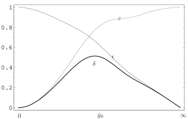
Figure 1: Schematic plot of the values of $\epsilon$, $\varepsilon$, and $\delta$ as functions of the distance between the central positions of the two Gaussian packets. This is the explicit zeroth order result for even-parity eigenstates. The horizontal distance in the figure is rescaled by the tangent function, $\bar{y}_{0}=\tan z$. Note that the explicit numerical value of $\delta$ is smaller than $1/2$.

For calculational convenience we introduce dimensionless operators $\hat{\pi}$ and $\hat{y}$ for momentum and position operators defined by

$$\hat{\pi}=\frac{\hat{p}}{\sqrt{\hbar\Omega}},~{}~{}\hat{y}=\frac{\hat{x}}{\sqrt{\hbar/\Omega}}.$$ (10)

Note also that $y_{0}=x_{0}\sqrt{\Omega/\hbar}$ relates the two parameters $\epsilon$ and $\varepsilon$ by

$$2\epsilon^{2}y_{0}^{2}=\varepsilon.$$ (11)

The commutation relation between $\hat{y}$ and $\hat{\pi}$ is

$$[\hat{y},\hat{\pi}] = i,$$ (12)

and the localization condition (7) becomes

$$\langle\hat{y}\rangle\sim 0,~{}~{}\langle(\hat{y}^{2}-y_{0}^{2})^{2}\rangle\sim\frac{1}{\epsilon^{2}},~{}~{}\langle\hat{\pi}\rangle\sim 0,~{}~{}\langle\hat{\pi}^{2}\rangle\sim\frac{1}{2}.$$ (13)

The expectation value of $\hat{y}^{2}$ is explicitly given by

$$\langle y^{2}\rangle=\frac{\langle\hat{x}^{2}\rangle}{2\hbar/(2\Omega)}=\frac{\bar{x}^{2}}{2x_{\Omega}^{2}}=\frac{1}{2\epsilon^{2}}.$$ (14)

For later use, we introduce some operators of $O(\epsilon^{0})$ and $O(\varepsilon^{0})$,

$$T_{1}^{0}=\sqrt{2}\hat{\pi},~{}~{}T_{0}^{1}=\sqrt{2}\epsilon\hat{y},~{}~{}T_{2}^{0}=2\hat{\pi}^{2},~{}~{}T_{0}^{2}=\epsilon(\hat{y}^{2}-y_{0}^{2}),~{}~{}T_{1}^{1}=\epsilon\{\hat{\pi},\hat{y}\}_{+},~{}~{}T_{0}^{4}=\epsilon^{2}(\hat{y}^{2}-y_{0}^{2})^{2},$$ (15)

which will be useful in describing the bi-centered systems.

II.2 Hamiltonian for variational approximation

We now consider a quartic oscillator, which will be used as a basis for the variational approximation, described by the Hamiltonian:

$$H_{0}=\frac{\hbar\Omega}{2}H_{m}+V_{0};~{}~{}~{}~{}H_{m}=\frac{1}{2}T_{2}^{0}+\frac{v_{2}\epsilon}{\epsilon_{0}^{2}}T_{0}^{2}+\frac{\bar{\lambda}\varepsilon}{2}T_{0}^{4},$$ (16)

where $V_{0}$ is the potential value at $\hat{y}=y_{0}$ and the subscript in $H_{0}$ denotes that this Hamiltonian will be used as a $0^{th}$ order form for the variational perturbative expansion of double-well and anharmonic oscillators. The constant $\epsilon_{0}$ is the value of $\epsilon$ in the harmonic oscillator limit, $y_{0}=0$. Explicitly, $\epsilon_{0}=1$ for $|0_{E}\rangle_{0}$ and $\epsilon_{0}=1/\sqrt{3}$ for $|0_{O}\rangle_{0}$. Note that this is one of the most general form of quartic Hamiltonian if $\Omega$ and $y_{0}$ are chosen arbitrarily. Note also that only one of the three quantities $\epsilon$, $\varepsilon$, and $y_{0}$ is an independent variable because of Eqs. (8), (11), and (14). Since we are to use the ground states of (16) as trial wavefunctions for the variational approximation for the Hamiltonian (2), we have two variational parameters, $\Omega$ and $y_{0}$.

The coefficients ($v_{2}$, $\bar{\lambda}$) in the Hamiltonian (16) can be written in terms of the above mentioned parameters by considering the two limiting cases, the harmonic oscillator ($y_{0}=0$) and the infinitely-separated ($y_{0}\rightarrow\infty$) double-well limits.

In the harmonic oscillator limit, the ground state is given by a Gaussian packet. The exact frequency is given by $\Omega=\omega$ and there is no quartic potential in the Hamiltonian. Therefore, the Hamiltonian (16) becomes that of the harmonic oscillator with correct frequency $\omega$ if

$$\mbox{harmonic oscillator limit}~{}(\varepsilon\rightarrow 0,~{}~{}\epsilon\rightarrow\epsilon_{0}):\left\{\begin{tabular}[]{l}$v_{2}(y_{0}\rightarrow 0)=1,$\\ $\bar{\lambda}(y_{0}\rightarrow 0)=\mbox{finite number}$.\\ \end{tabular}\right.$$

On the other hand, for the ground state of the infinitely separated double-well limit ($y_{0}\rightarrow\infty$), we have $\epsilon=0$ and $\varepsilon=1$ and the $T_{0}^{2}$ term disappears since $\epsilon$ vanishes. Each packet at $x=\pm x_{0}$ evolves as if it is a free harmonic oscillator. The frequency of each packets is determined by the second derivative of the potential with respect to $x$ at the bottom of the potential. This determines $\Omega^{2}=2\lambda x_{0}^{2}=2\lambda\bar{x}^{2}$. Therefore, the coefficient $\bar{\lambda}$ of $T_{0}^{4}$ term must be $1$ in this limit:

$$\mbox{infinitely separated double-well limit}~{}(\varepsilon\rightarrow 1,~{}~{}\epsilon\rightarrow 0):\left\{\begin{tabular}[]{l}$v_{2}(y_{0}\rightarrow\infty)=\mbox{finite number},$\\ $\bar{\lambda}(y_{0}\rightarrow\infty)=1$.\\ \end{tabular}\right.$$

With these observations, it is clear that the constants $v_{2}$ and $\bar{\lambda}$ are of $O(\delta^{0})$. The values $v_{2}$ and $\bar{\lambda}$ become important at the harmonic oscillator limit and the infinitely separated double-well limit, respectively. For both limits, therefore, we may set

$$v_{2}=1=\bar{\lambda},$$ (19)

for the zeroth order approximate Hamiltonian $H_{0}$. With the values of $v_{2}$ and $\bar{\lambda}$ of Eq. (19), the Hamiltonian (16) still describes the most general anharmonic and double-well oscillators since $\Omega$ and $y_{0}$ are free parameters.

II.3 Zeroth order results

As we have discussed in the previous section, we try to find an annihilation operator $\hat{A}$ and a creation operator $\hat{A}^{\dagger}$ to $O(\delta^{0})$ in this subsection. Since we want to find the operators as even functions of the bi-centered operators we try the simplest ansatz for the zeroth order operator ${\hat{\cal A}}$:

$${\hat{\cal A}} = u(t)T_{0}^{2}+v(t)T_{1}^{1}+w(t)T_{2}^{0}.$$

To the zeroth order, one can easily find that the LvN equation, $\displaystyle i\hbar\frac{d{\hat{\cal A}}(\hat{p},\hat{x},t)}{dt}=i\hbar\frac{\partial{\hat{\cal A}}}{\partial t}+[{\hat{\cal A}},H_{0}]=0$, becomes a matrix differential equation of the form

$$\frac{d{\bf A}(t)}{dt}=\frac{i\Omega}{2}M{\bf A}(t),~{}~{}~{}~{}{\bf A}(t)=\left(\begin{tabular}[]{c}$u$\\ $v$\\ $w$\end{tabular}\right),$$

where $M$ is a $(3\times 3)$ matrix determined by the commutator of ${\hat{\cal A}}$ and $H_{m}$ of Eq. (16). For the time-independent case, the differential equation can be solved by a simple matrix eigenvalue equation by setting $\displaystyle{\bf A}(t)=e^{i\zeta\Omega t}{\bf A}(t=0)$. Explicit calculation of the commutator $[{\hat{\cal A}},H_{m}]$ gives the matrix $M$:

$$M=-i\left(\begin{tabular}[]{ccc}0&0&$2\epsilon^{2}/\epsilon_{0}^{2}+\varepsilon^{2}$\\ 0&0&$-\epsilon$\\ $-1$&$2\epsilon/\epsilon_{0}^{2}$&0\\ \end{tabular}\right).$$

The eigenvalues of $M$ are given by the solution $\zeta$ of

$$-\zeta(\zeta^{2}-\alpha^{2})=0,$$

where

$$\alpha=\sqrt{\frac{4\epsilon^{2}}{\epsilon_{0}^{2}}+\varepsilon^{2}}.$$ (22)

We have three different $\zeta$ eigenvalues, $(0,\pm\alpha)$. The $\zeta=0$ solution is, in fact, the Hamiltonian itself. Since what we want to find in this section is the creation and the annihilation operators, we do not try to analyze it here.

The other two solutions with eigenvalues $\zeta=\pm\alpha$ denote, in fact, a set of operators ${\hat{\cal A}}$ and ${\hat{\cal A}}^{\dagger}$. If we demand ${\hat{\cal A}}$ being a negative frequency mode, we have

$${\hat{\cal A}} \equiv b_{0}e^{i\alpha\Omega t}\hat{\mathfrak{a}}\,;\quad\quad\hat{\mathfrak{a}}=-i\nu^{2}T_{0}^{2}+T_{1}^{1}+\frac{i\epsilon}{\alpha}T_{2}^{0},$$ (23)

$${\hat{\cal A}}^{\dagger} \equiv b_{0}e^{-i\alpha\Omega t}\hat{\mathfrak{a}}^{\dagger}\,;\quad\quad\hat{\mathfrak{a}}^{\dagger}=i\nu^{2}T_{0}^{2}+T_{1}^{1}-\frac{i\epsilon}{\alpha}T_{2}^{0},$$

where $b_{0}$ is a normalization constant to be determined later and $\nu$ is

$$\nu^{2}=\frac{2\epsilon^{2}/\epsilon_{0}^{2}+\varepsilon^{2}}{\alpha}.$$ (24)

These are the zeroth order annihilation and creation operators we were looking for. Thus the operator ${\hat{\cal A}}$ satisfies

$$\frac{d{\hat{\cal A}}(t,\hat{p}(t),\hat{x}(t))}{dt}\simeq 0,$$

where $\simeq$ denotes ”the same up to $O(\delta^{0})$” and ${\hat{\cal A}}$ and ${\hat{\cal A}}^{\dagger}$ are the zeroth order invariant operators. The explicit algebra satisfied by the operators ${\hat{\cal A}}$ and ${\hat{\cal A}}^{\dagger}$ will be shown in the next subsection.

II.4 Algebraic properties of the zeroth order invariant operators

In the previous subsection, we obtained the annihilation and the creation operators which satisfy the zeroth order LvN equation. We expect that the zeroth order solution of the LvN equation has the structure of a generalized deformed oscillator as we have pointed out in the introduction. In this subsection, we show that there exist well defined algebraic properties of the operators ${\hat{\cal A}}$ and ${\hat{\cal A}}^{\dagger}$.

Using Eqs. (15) and (12), we find the commutator of the operators ${\hat{\cal A}}$ and ${\hat{\cal A}}^{\dagger}$:

$$\frac{[{\hat{\cal A}},{\hat{\cal A}}^{\dagger}]}{4b_{0}^{2}} = \nu^{2}\varepsilon+\frac{4\epsilon^{2}H_{m}}{\alpha}+\frac{2\delta}{\alpha}\left(\varepsilon T_{0}^{2}-\epsilon T_{0}^{4}\right)$$

$$= \alpha\varepsilon+\frac{4\epsilon^{2}H_{m}}{\alpha}+O(\delta).$$

The anticommutator of the operators ${\hat{\cal A}}$ and ${\hat{\cal A}}^{\dagger}$ is

$$\frac{\{{\hat{\cal A}},{\hat{\cal A}}^{\dagger}\}_{+}}{4b_{0}^{2}} = \frac{3\epsilon^{2}}{2}+\varepsilon\left(\frac{1}{2}T_{2}^{0}+\frac{\varepsilon}{2}T_{0}^{4}\right)+\frac{2\epsilon^{2}}{\alpha^{2}}\left(\frac{1}{2}T_{2}^{0}+\frac{\epsilon}{\epsilon_{0}^{2}}T_{0}^{2}\right)^{2}$$

$$= \varepsilon H_{m}+\frac{\epsilon^{2}}{2}\left(3+\frac{4H_{m}^{2}}{\alpha^{2}}\right)+O(\delta).$$

The algebraic structure of the deformed oscillator will be apparent by introducing a structure function $\Phi_{0}(\hat{N}_{0})$ of the form

$$\Phi_{0}(\hat{N}_{0}) = 4b_{0}^{2}\left({\cal E}_{+}\hat{N}_{0}+4\epsilon^{2}\hat{N}_{0}^{2}\right).$$ (27)

By comparing Eqs. (II.4), (II.4), and (27) with Eq. (1), we have

$${\cal E}_{+} = \alpha\varepsilon+4\epsilon^{2}\left(\frac{{\cal E}_{0}}{\alpha}-1\right).$$

The constant ${\cal E}_{0}$ is determined by the condition $\Phi_{0}(0)=0$. With (II.4) and (II.4), the condition reads

$$\alpha\varepsilon\left(\frac{{\cal E}_{0}}{\alpha}-1\right)+2\epsilon^{2}\left[\left(\frac{{\cal E}_{0}}{\alpha}-1\right)^{2}-\frac{1}{4}\right]\simeq 0.$$ (28)

This equation determines the energy eigenvalues in both the harmonic oscillator and the infinitely separated double-well limits. For the infinitely separated double-well limit ($y_{0}\rightarrow\infty,~{}\epsilon\rightarrow 0$), we have ${\cal E}_{0}=\alpha$ and for the harmonic oscillator limit ($y_{0}\rightarrow 0,~{}\varepsilon\rightarrow 0$), we have two different solution ${\cal E}_{0}=3\alpha/2,~{}\alpha/2$. These two eigenvalues correspond to the energy eigenvalues of the odd-parity and the even-parity ground states. The rescaled ground state energy $E_{0}$ in Table 1, which is determined by Eq. (63) below, satisfies this condition (28).

The structure function (27) and the number operator $\hat{N}_{0}$,

$$\hat{N}_{0}=\frac{H_{m}-{\cal E}_{0}}{2\alpha},$$ (29)

satisfy the conditions for the generalized deformed oscillator, Eq. (1), since

$${\hat{\cal A}}^{\dagger}{\hat{\cal A}}\simeq\Phi_{0}(\hat{N}_{0}),~{}~{}{\hat{\cal A}}{\hat{\cal A}}^{\dagger}\simeq\Phi_{0}(\hat{N}_{0}+1).$$ (30)

The Hamiltonian can be written in terms of the number operator $\hat{N}_{0}$ as

$$H\simeq\frac{\hbar\Omega}{2}(2\alpha\hat{N}_{0}+{\cal E}_{0})+V(x_{0}).$$ (31)

Therefore, the ground state energy is given by $\displaystyle\frac{\hbar\Omega}{2}{\cal E}_{0}+V(x_{0})$ and the energy difference between two nearby states in each parity sector is $\alpha\hbar\Omega$.

The yet undetermined quantity $b_{0}$ in Eq. (23) is fixed by imposing $[{\hat{\cal A}},{\hat{\cal A}}^{\dagger}]|0_{E/O}\rangle_{0}=|0_{E/O}\rangle_{0}$. This gives

$$\Phi_{0}(1)\equiv 1~{}~{}~{}\Longrightarrow~{}~{}~{}b_{0}^{2}=\frac{1}{4({\cal E}_{+}+4\epsilon^{2})}.$$ (32)

Note also that due to the LvN equation (3), (16), and the definition of $\hat{N}_{0}$ (29), we have the desired commutation relation:

$$~{}[{\hat{\cal A}},\hat{N}_{0}]\simeq{\hat{\cal A}},\quad~{}~{}[{\hat{\cal A}}^{\dagger},\hat{N}_{0}]\simeq-{\hat{\cal A}}^{\dagger}.$$ (33)

With these algebra and Eq. (27), the ground state $|0_{E/O}\rangle_{0}$ can be defined as an eigenstate of $\hat{N}_{0}$:

$${\hat{\cal A}}|0_{E/O}\rangle_{0}\simeq 0.$$ (34)

From Eq. (30) and the condition $\Phi_{0}(0)=0$, the number operator annihilates the ground states:

$$\hat{N}_{0}|0_{E/O}\rangle_{0}\equiv|0_{E/O}\rangle_{0}\Phi_{0}^{-1}(0)=0.$$ (35)

The $n^{th}$ excited states are generated by the formula:

$$|n_{E/O}\rangle_{0}=\frac{(\hat{\cal A}^{\dagger})^{n}}{\sqrt{[n]_{0}!}}|0_{E/O}\rangle_{0},$$ (36)

where

$$[n]_{0}!\equiv\prod^{n}_{k=1}[k]_{0}=\prod_{k=1}^{n}\Phi_{0}(k).$$ (37)

The states $|n_{E}\rangle_{0}$ and $|n_{O}\rangle_{0}$ are the $(2n)^{th}$ and the $(2n+1)^{th}$ excited states with even and odd parities of the anharmonic and the double-well oscillator. Due to Eqs. (30) and (33), the states have the eigenvalues $n_{E/O}$ for $\hat{N}_{0}$:

$$\hat{N}_{0}|n_{E/O}\rangle_{0}\simeq n_{E/O}|n_{E/O}\rangle_{0}.$$ (38)

Moreover, these eigenstates are orthonormal to each other to the zeroth order:

$${}_{0}\langle n_{E/O}|m_{E/O}\rangle_{0}\simeq\delta_{nm}.$$ (39)

Eqs. (27), (29), (30), (33), and (34) constitute the conditions for a generalized deformed oscillator which possesses a Fock space of eigenvectors $|0_{E/O}\rangle_{0},~{}|1_{E/O}\rangle_{0},~{}\cdots,|n_{E/O}\rangle_{0},\cdots$ of the number operator $\hat{N}_{0}$. Further specification of $\hat{A}$ to higher order is possible perturbatively, which is the purpose of Sec. IV.

III Variational approximation

In the previous section we have obtained a zeroth order invariant creation and annihilation operators which satisfies the LvN equation for the zeroth order Hamiltonian (16) which depends on two arbitrary parameters, $\Omega$ and $y_{0}$. By using the ground state of the zeroth order Hamiltonian (16) as a trial wavefunction we develop, in this section, a variational approximation of the anharmonic and the double-well oscillators. We then compare our result with those of other approximation methods.

In coordinate space $y$, the eigenstate $\Psi(y)$, which satisfies ${\hat{\cal A}}\Psi(y)=0$, is given by the linear combination of $e^{-\alpha y^{2}}H_{m}(\beta y)$ and the confluent hypergeometric function ${}_{1}F_{1}$, which give difficulty in analytic manipulations. Therefore, we propose to use an operator $\hat{a}_{0}$ which is equivalent to ${\hat{\cal A}}$ up to the zeroth order but have simpler ground state:

$$\hat{a}_{0}\equiv-2i\epsilon\hat{a}_{+}\hat{a}_{-}\simeq-2i\epsilon\hat{a}_{+}\hat{a}_{-}+\frac{i\varepsilon\delta}{2\nu^{2}\alpha^{2}}T_{2}^{0}=\frac{{\hat{\cal A}}}{b_{0}e^{i\alpha\Omega t}}=\hat{\mathfrak{a}},$$

where

$$\hat{a}_{\pm}=\frac{i}{\sqrt{2}\nu}\hat{\pi}+\frac{\nu}{\sqrt{2}}(\hat{y}\mp y_{0})$$ (40)

are the annihilation operators of harmonic oscillators centered around $y=\pm y_{0}$. The new operator is explicitly written as

$$\hat{a}_{0} = -i\nu^{2}T_{0}^{2}+T_{1}^{1}+\frac{i\epsilon}{2\nu^{2}}T_{2}^{0}.$$ (41)

The operators $\hat{\pi}$ and $\hat{y}$ are related to $\hat{a}_{\pm}$ by

$$\hat{\pi} = -\frac{i\nu}{\sqrt{2}}(\hat{a}_{\pm}-\hat{a}_{\pm}^{\dagger}),$$ (42)

$$-\sqrt{2}\nu y_{0} = \hat{a}_{+}-\hat{a}_{-},$$

$$\hat{y} = \pm y_{0}+\frac{\hat{a}_{\pm}+\hat{a}_{\pm}^{\dagger}}{\sqrt{2}\nu}.$$

Thus ${\hat{\cal A}}$ is equivalent to the zeroth order to the product of the two annihilation operators of harmonic oscillators centered around $y=\pm y_{0}$. Note that the annihilation operators $\hat{a}_{\pm}$ and the creation operators $\hat{a}_{\pm}^{\dagger}$ satisfy the standard commutation relation

$$[\hat{a}_{\pm},\hat{a}_{\pm}^{\dagger}]=1,\quad\quad[\hat{a}_{+},\hat{a}_{-}]=0.$$ (43)

Consider the states $|\pm\rangle$ annihilated by $\hat{a}_{\pm}$,

$$\hat{a}_{\pm}|\pm\rangle=0.$$ (44)

The wave-functions for states $|\pm\rangle$ are

$$\Psi_{\pm}(y)\equiv\langle y|\pm\rangle={\nu^{1/2}\over\pi^{1/4}}e^{-\nu^{2}(y-y_{0})^{2}/2},$$

which determine the overlap $\langle+|-\rangle$:

$$\langle+|-\rangle=e^{-\nu^{2}y_{0}^{2}}.$$

Since both of the two states $|\pm\rangle$ are annihilated by $\hat{a}_{0}$, the approximate ground states of even or odd parity, $|0_{E/O}\rangle$, which are annihilated by $\hat{a}_{0}$, are given by the linear combinations,

$$|0_{E}\rangle_{0}=\frac{1}{M_{E}}\frac{|+\rangle+|-\rangle}{\sqrt{2}},~{}~{}|0_{O}\rangle_{0}=\frac{1}{M_{O}}\frac{|+\rangle-|-\rangle}{\sqrt{2}}.$$ (45)

The normalization constants are

$$M_{E}^{2}=1+\langle+|-\rangle=1+e^{-\nu^{2}y_{0}^{2}},\quad\quad M_{O}^{2}=1-\langle+|-\rangle=1-e^{-\nu^{2}y_{0}^{2}}.$$ (46)

The ground states (45) satisfy

$${}_{0}\langle n_{E/O}|0_{E/O}\rangle_{0}=0,\quad\mbox{ for }n\neq 0,$$

where the excited states $|n_{E/O}\rangle_{0}$ are generated by the successive action of $\hat{a}_{0}^{\dagger}$ on the ground states. We thus have constructed the set of operators $(\hat{a}_{0},\hat{a}_{0}^{\dagger})$ and the even and odd ground states $(|0_{E}\rangle_{0},|0_{O}\rangle)$, which properly describe both the anharmonic and double-well oscillator simultaneously to the zeroth order in $\delta$.

The expectation values of operators with respect to the states $|0_{E/O}\rangle_{0}$ can be obtained algebraically by using Eqs. (42), (43), and (44). For example, the expectation value of $T_{2}^{0}$ is

$${}_{0}\langle 0_{E/O}|T_{2}^{0}|0_{E/O}\rangle_{0} = -\frac{1}{2N^{2}}(\langle+|\pm\langle-|)(\hat{a}_{+}-\hat{a}_{+}^{\dagger})^{2}(|+\rangle\pm|-\rangle)=\nu^{2}T_{E/O},$$ (47)

where upper (lower) sign refers to the even (odd) parity case and

$$T_{E/O}(\nu y_{0}) \equiv 1-2\nu^{2}y_{0}^{2}C_{E/O}=1\mp\frac{2\nu^{2}y_{0}^{2}}{e^{\nu^{2}y_{0}^{2}}\pm 1}.$$ (48)

Starting from $1$, $T_{E}$ decreases to $0.45$ at $\nu y_{0}=1.1$ and then increases again to $1$ as $\nu y_{0}$ increases. On the other hand, $T_{O}$ continuously decreases from $3$ to $1$ as $\nu y_{0}$ increases. The functions $C_{E/O}$ are

$$C_{E}(\nu y_{0}) = \langle+|-\rangle/M_{E}^{2}=(e^{\nu^{2}y_{0}^{2}}+1)^{-1},$$

$$C_{O}(\nu y_{0}) = -\langle+|-\rangle/M_{O}^{2}=-(e^{\nu^{2}y_{0}^{2}}-1)^{-1}.$$

As shown in this equation, the expectation values for the even and the odd ground states take similar form except for the indices in $C_{E/O}$. From now on, $C$ will denote both of $C_{E/O}$ if not specified. This convention is applied to all other variables such as $\epsilon$, $\nu$, $M$, $E_{0}$, $T$, and $R$ defined below. The expectation value of $T_{0}^{2}$ is

$${}_{0}\langle 0_{E/O}|T_{0}^{2}|0_{E/O}\rangle_{0} = \frac{\epsilon}{2\nu^{2}}T\,.$$ (49)

The formal identity $\bar{x}^{2}\equiv\langle(x^{2}-x_{0}^{2})\rangle+x_{0}^{2}$ leads to the following relation among parameters,

$$\frac{2\nu^{2}y_{0}^{2}}{M^{2}}+1=\frac{(\nu y_{0})^{2}}{(\epsilon y_{0})^{2}}.$$ (50)

Since the normalization constant $M$ is a function of $\nu y_{0}$, this equation determines $\epsilon y_{0}$ in terms of $\nu y_{0}$ or vice versa. This equation has interesting implications on the limiting cases. In the limit $y_{0}\rightarrow 0$, Eq. (50) determines $\epsilon_{E}=1$ and $\epsilon_{O}=1/\sqrt{3}$. On the other hand, in the limit $y_{0}\rightarrow\infty$, we have $\epsilon\simeq 1/(\sqrt{2}y_{0})$ irrespective of the parity of the states. The equation (50) can be rewritten for $\varepsilon$ as a function of $\bar{y}_{0}=\nu y_{0}$:

$$\varepsilon(\bar{y}_{0})=2\epsilon^{2}y_{0}^{2}=\frac{2\bar{y}_{0}^{2}}{1+\frac{2\bar{y}_{0}^{2}}{1\pm e^{-\bar{y}_{0}^{2}}}}.$$ (51)

In addition, $\epsilon$ can be written as a function of $\bar{y}_{0}$, from Eqs. (22), (24), and (51), as

$$\frac{\epsilon(\bar{y}_{0})}{\epsilon_{0}\varepsilon(\bar{y}_{0})} = \frac{\sqrt{3}}{\sqrt{2}}\left[-2+\frac{3\bar{y}_{0}^{4}+1}{g^{1/3}(\bar{y})}+g^{1/3}(\bar{y})\right]^{-\frac{1}{2}};$$ (52)

$$g(\bar{y}) = 1+18\bar{y}_{0}^{4}+3\sqrt{3}\bar{y}_{0}^{2}\sqrt{1+11\bar{y}_{0}^{4}-\bar{y}_{0}^{8}}.$$

The explicit values of $\varepsilon$, $\epsilon$, and $\delta=\varepsilon\epsilon$ are plotted in Fig. 1.

We also calculate the expectation value of the quartic part of the Hamiltonian:

$${}_{0}\langle 0_{E/O}|T_{0}^{4}|0_{E/O}\rangle_{0} = \frac{\epsilon^{2}}{\nu^{4}}\left[\frac{3+8\nu^{2}y_{0}^{2}}{4}+\nu^{2}y_{0}^{2}\left(\nu^{2}y_{0}^{2}-3\right)C\right]$$

$$= \frac{\epsilon^{2}}{4\nu^{4}}\left[3+8\nu^{2}y_{0}^{2}\pm\frac{4\nu^{2}y_{0}^{2}\left(\nu^{2}y_{0}^{2}-3\right)}{e^{\nu^{2}y_{0}^{2}}\pm 1}\right].$$

III.1 Effective Potential

As in the Gaussian approximation, in which the ground state of $\displaystyle H=\frac{p^{2}}{2}+\frac{\Omega^{2}}{2}x^{2}$ is chosen to be the trial wavefunction for the Hamiltonian (2), we use the states (45), which are the $O(\delta^{0})$ even and odd ground states of the Hamiltonian (16), as trial wavefunctions for the variational approximation for the Hamiltonian (2). Therefore, the $y_{0}\rightarrow 0$ limit of our approximation becomes the Gaussian approximation, and the approximation with $y_{0}=1/(\sqrt{2}\epsilon)$ limit describes a double Gaussian approximationkovner ; cooper . For this variational approximation we write the Hamiltonian (2) of a general anharmonic $\omega^{2}>0$ or a double-well $\omega^{2}<0$ oscillator in terms of operators defined in Eq. (15):

$$H = \frac{\hat{p}^{2}}{2}+\frac{\omega^{2}}{2}\hat{x}^{2}+\frac{\lambda}{4}\hat{x}^{4}+\frac{\omega^{4}}{4\lambda}\theta(-\omega^{2})$$

$$= \frac{\hbar\Omega}{2}\left[\frac{1}{2}T_{2}^{0}+\frac{1}{\epsilon}\left(\frac{\omega^{2}}{\Omega^{2}}+\frac{\lambda x_{0}^{2}}{\Omega^{2}}\right)T_{0}^{2}+\frac{\lambda\hbar}{2\Omega^{3}\epsilon^{2}}T_{0}^{4}\right]+V(x_{0}),$$

$$= \frac{\hbar|\omega|\Omega_{r}}{2}\left[\frac{1}{2}T_{2}^{0}+\frac{1}{\epsilon}\left(\frac{\mbox{sign}(\omega^{2})}{\Omega_{r}^{2}}+\frac{2\lambda_{r}y_{0}^{2}}{\Omega_{r}^{3}}\right)T_{0}^{2}+\frac{\lambda_{r}}{\Omega_{r}^{3}\epsilon^{2}}T_{0}^{4}\right]+V(x_{0}),$$

where the potential $V(x_{0})$ is

$$V(x_{0}) = \frac{\omega^{2}x_{0}^{2}}{2}+\frac{\lambda x_{0}^{4}}{4}+\frac{\omega^{4}}{4\lambda}\theta(-\omega^{2})=\frac{\hbar|\omega|\Omega_{r}}{2}\left(\mbox{sign}(\omega^{2})\frac{y_{0}^{2}}{\Omega_{r}^{2}}+\frac{\lambda_{r}y_{0}^{4}}{\Omega_{r}^{3}}+\frac{\theta(-\omega^{2})}{4\lambda_{r}\Omega_{r}}\right).$$ (55)

In this equation the theta function, $\theta(-\omega^{2})$, is included to make the lowest energy of the potential vanish for $\omega^{2}<0$, and $x_{0}=\sqrt{\hbar/\Omega}\,y_{0}$, and the dimensionless parameters $\lambda_{r}$ and $\Omega_{r}$ are defined by

$$\lambda_{r}=\frac{\lambda\hbar}{2|\omega|^{3}},\quad~{}\Omega_{r}={\Omega\over|\omega|}.$$ (56)

From Eqs. (47), (49), and (III), the expectation values of the Hamiltonian (III.1) with respect to the ground states $|0_{E}\rangle$ and $|0_{O}\rangle$ in Eq. (45) become

$$\frac{2\langle H\rangle}{\hbar|\omega|}=\frac{\Omega_{r}\nu^{2}T}{2}+\mbox{sign}(\omega^{2})\frac{T+2\nu^{2}y_{0}^{2}}{2\Omega_{r}\nu^{2}}+\frac{\lambda_{r}}{4(\Omega_{r}\nu^{2})^{2}}R(\nu y_{0})+\frac{\theta(-\omega^{2})}{4\lambda_{r}},$$ (57)

where we have used Eq. (50) to eliminate $\epsilon$ for $\nu$, and

$$R(\nu y_{0})=3+12\nu^{2}y_{0}^{2}+4\nu^{4}y_{0}^{4}-4\nu^{2}y_{0}^{2}(3+\nu^{2}y_{0}^{2})C=3+\frac{4\nu^{2}y_{0}^{2}(3+\nu^{2}y_{0}^{2})}{1\pm e^{-\nu^{2}y_{0}^{2}}}.$$ (58)

The function $R_{E}~{}(R_{O})$ monotonically increases from $3~{}(15)$ as $\nu y_{0}$ increases. Note that the rescaling,

$$\Omega_{r}\nu^{2}\equiv\bar{\Omega},\quad\quad\nu y_{0}\equiv\bar{y}_{0}\,,$$ (59)

completely remove the $\nu$ dependence on the expectation values since $T$ defined by (48) is the function only of $\nu y_{0}$. The value of $\nu$ only affects the relation between $\epsilon$ and $y_{0}$ through Eq. (50). With these new parameters, the expectation value (57) becomes

$$\frac{2\langle H\rangle}{\hbar|\omega|}=\frac{\bar{\Omega}T(\bar{y}_{0})}{2}+\mbox{sign}(\omega^{2})\frac{T(\bar{y}_{0})+2\bar{y}_{0}^{2}}{2\bar{\Omega}}+\frac{\lambda_{r}}{4\bar{\Omega}^{2}}R(\bar{y}_{0})+\frac{\theta(-\omega^{2})}{4\lambda_{r}}.$$ (60)

The variation of (60) with respect to $\bar{\Omega}$ gives the gap equation,

$$\bar{\Omega}^{3}-\mbox{sign}(\omega^{2})\left(1+\frac{2\bar{y}_{0}^{2}}{T(\bar{y}_{0})}\right)\bar{\Omega}-\frac{\lambda_{r}R(\bar{y}_{0})}{T(\bar{y}_{0})}=0,$$ (61)

which determines non-trivial unique positive solution for $\bar{\Omega}$

$$\bar{\Omega}(\bar{y}_{0}) = \left(\frac{2}{3}\right)^{1/3}\left[\frac{D^{1/3}}{3\cdot 2^{1/3}}+\mbox{sign}(\omega^{2})\frac{1+\frac{2\bar{y}_{0}^{2}}{T(\bar{y}_{0})}}{D^{1/3}}\right];$$ (62)

$$D = \frac{9\lambda_{r}R(\bar{y}_{0})}{T(\bar{y}_{0})}+2\sqrt{3}\sqrt{-\mbox{sign}(\omega^{2})\left(1+\frac{2\bar{y}_{0}^{2}}{T(\bar{y}_{0})}\right)^{3}+\frac{27}{4}\frac{\lambda_{r}^{2}R^{2}(\bar{y}_{0})}{T^{2}(\bar{y}_{0})}},$$

for all values of $\omega^{2}$ irrespective of its sign if $\lambda\geq 0$. We set this solution be $\bar{\Omega}(\bar{y}_{0})$. Note that the gap equation (61) takes similar form as that of the variational Gaussian approximation except for the dependence of the coefficients on $\bar{y}_{0}$.

We thus have the effective potential as a function of $\bar{y}_{0}$ by inserting the solution (62) to Eq. (60):

$$\frac{2V_{eff}(\bar{y}_{0})}{\hbar|\omega|} = \bar{\Omega}(\bar{y}_{0})T(\bar{y}_{0})-\frac{\lambda_{r}}{4\bar{\Omega}^{2}(\bar{y}_{0})}R(\bar{y}_{0})+\frac{\theta(-\omega^{2})}{4\lambda_{r}}.$$ (63)

The functional dependence of $V_{eff}(\bar{y}_{0})$ on $\bar{y}_{0}$ is shown in Fig. 2 for a couple of values of $\lambda_{r}$.

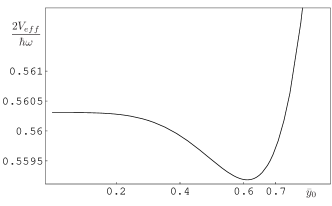
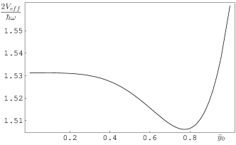
Figure 2: Effective potential $\displaystyle\frac{2V_{eff}(\bar{y}_{0})}{\hbar|\omega|}$ as a function of $\bar{y}_{0}$ for the coupling constants $\lambda_{r}=2$ (left) and $\lambda_{r}=20$ (right) for $\omega^{2}>0$.
The energy decreases very slowly for $\bar{y}_{0}\ll 1$ and increases for large $\bar{y}_{0}$. Therefore, there exists a unique minimum of $V_{eff}(\bar{y}_{0})$ for positive $\bar{y}_{0}$. Since the graphs are nearly flat for $\bar{y}_{0}\ll 1$, $y_{c}$ increases very fast for small $\lambda_{r}$ as depicted in Fig. 3.

We write the value $\bar{y}_{0}$ that minimizes the effective potential (63) as $y_{c}$:

$$\left.\frac{dV_{eff}(\bar{y}_{0})}{d\bar{y}_{0}}\right|_{\bar{y}_{0}=y_{c}}=0.$$ (64)

Then, the ground state energy is given by $V_{eff}(y_{c})$. With this $y_{c}$, $\bar{\Omega}(y_{c})$ is determined from Eq. (62), and $\epsilon(y_{c})$ and $\varepsilon(y_{c})$ are determined from Eqs. (51) and (52). With these results the annihilation operator (41) is uniquely determined. In Appendix A, we explicitly analyze the variational equation, Eq. (64) and the results for positive $\omega^{2}$ are shown in Fig. 3.

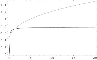
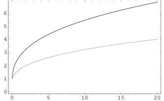
Figure 3: Behavior of ground state energy ($\displaystyle\frac{2V_{eff}(y_{c})}{\hbar|\omega|}$), $y_{c}$, $\bar{\Omega}$, and $\Omega_{G}$ as functions of $\lambda_{r}$ (horizontal axis) for $\omega^{2}>0$.
The left figure shows the energy (grey curve) and $y_{c}$ (black curve) as functions of $\lambda_{r}$. On the right shows the behavior of the present $\bar{\Omega}(\lambda_{r})$ (black curve) compared to $\Omega_{G}(\lambda_{r})$ (grey curve), the Gaussian value. As seen in this figure, the effective frequency $\bar{\Omega}$ is much larger than the Gaussian value $\Omega_{G}$ for $\lambda_{r}\gg 1$.

In general we have nonzero $y_{c}$ for positive $\lambda$. We present the energy eigenvalues of the even and odd ground states and $\varepsilon$ for several values of the coupling strength in Table 1. As one can see in Table 1, even for a very small coupling, such as $\lambda_{r}\sim 2\cdot 10^{-3}$, we have non-negligible $y_{c}$ value, $\displaystyle\varepsilon=y_{c}^{2}/\bar{y}^{2}\sim 0.1$. Since we have $y_{c}=0$ in the Gaussian approximation, non-vanishing $y_{c}$ measures the departure from the Gaussian results. This is measured by the value $\varepsilon$ in Table 1. The energy eigenvalues of our zeroth order approximation is closer to the exact values than the 2nd order perturbative results of the approximation methods based on the Gaussian approximation for vast range of couplings.

Table 1: The explicit energy eigenvalues for anharmonic and double-well oscillators for several values of coupling strength. ‘Caswell’ and ‘NGAS’ refer to the results of Ref. ref7 and mahapatra , respectively. ‘Exact’ implies the exact numerical result.

	$\omega^{2}>0$						$\omega^{2}<0$
$\lambda\hbar/(2|\omega|^{3})$	0.002	0.02	0.2	2	20	200	200	20	2	0.2
$\varepsilon$	0.1054	0.2824	0.5170	0.6419	0.6751	0.6824	0.6865	0.6940	0.7296	0.8705
$E_{0}/(\hbar\omega)$	0.5007	0.5072	0.5592	0.8041	1.5062	3.134	3.0730	1.3793	0.5784	0.4767
Exact	0.5007	0.5072	0.5591	0.8038	1.5050	3.1314	3.0700	1.3800	0.5800	0.4702
NGAS(2nd)	0.5007	0.5072	0.5591	0.8032	1.5030	3.1266	3.0650	1.3752	0.5752	0.4606
$E_{1}/(\hbar\omega)$		1.5356	1.7696	2.7387	5.3240	11.193	11.0393	4.9984	2.0850	0.7713
Caswell			1.7695	2.7379	5.3216	11.187	11.002	5.0900	2.1800	0.7703
NGAS(2nd)			1.7694	2.7367	5.3177	11.178	11.024	4.9910	2.0800	0.7553

Finally, we consider when the wavefunction becomes aware of the transition of the potential from a single-well system to a double-well system in the sense that the wavefunction becomes concave from convex at $y=0$ turbiner . The second derivative of the ground state wavefunction at $y=0$ is given by

$$\left.\frac{\Psi_{0,E}^{\prime\prime}(y)}{\Psi_{0,E}(y)}\right|_{y=0}=\nu^{2}(\nu^{2}y_{0}^{2}-1),$$ (65)

which changes from negative to positive at $\nu^{2}y_{0}^{2}=1$. This equation combined with Eq. (50) determines the moment when a the second derivatives of the wavefunction at $y=0$ changes its sign:

$$\varepsilon=\frac{2(e+1)}{3e+1}\simeq 0.8123,~{}~{}\lambda_{r}\simeq 0.418.$$ (66)

This value of critical coupling is somewhat larger than the corresponding value (0.302) of Ref. turbiner in which the approximate eigenstates of double-well oscillator were analyzed by variational approximation with 5-variational parameters.

III.2 Weak coupling approximations

In this subsection, we study the weak coupling ($\lambda_{r}\ll 1$) limit of our result. We need the weak coupling limit for two reasons. First, the approximate energy (60) is too complex. To compare the result with others, it is convenient to consider various limiting cases. Secondly, to calculate higher order invariant operators, we need to understand the behaviors of the Hamiltonian (III.1) in various limits of our parameters. Explicitly, we need to know the orders of magnitudes of the coefficients $\displaystyle\left(\frac{\omega^{2}}{\Omega^{2}}+\frac{\lambda x_{0}^{2}}{\Omega^{2}}\right)\frac{1}{\epsilon}$ and $\displaystyle\frac{\lambda\hbar}{2\Omega^{3}\epsilon^{2}}$ of the quadratic and quartic parts, respectively, of the Hamiltonian (III.1) to construct higher order correction terms.

Before explicitly presenting the limiting case, let us first consider the Gaussian approximation limit ($y_{0}\rightarrow 0$) of our result. The ground state wavefunction, in this case, is a Gaussian. For this wavefunction, we have the root mean square value of the position operator, $\displaystyle\bar{x}=x_{\Omega}=\sqrt{\frac{\hbar}{2\Omega}}~{}(\sqrt{3}x_{\Omega})$, for the ground state (first excited state). Therefore, we have $T_{E}=1$, $\epsilon_{0,E}=1$, and $R_{E}=3$ for even parity case, and $T_{O}=3$, $\epsilon_{0,O}=1/\sqrt{3}$, and $R_{O}=5$ for odd parity case. The value of $\Omega$ is determined by the Gap equation:

$$\left(\Omega_{r}\right)^{3}-\Omega_{r}-\lambda_{r}R=0.$$

This gap equation is the same as that of the Gaussian approximation for the state $|0_{E}\rangle$. The gap equation for the state $|0_{O}\rangle$ is different from that of the Gaussian approximation since $R_{O}\neq R_{E}$. This difference makes the energy of the $1^{st}$ excited state different from that of the Gaussian approximation. The energies for both states are

$$E_{0,E/O}=\frac{\hbar\Omega_{E/O}T_{E/O}}{2}\left(1-\frac{\lambda\hbar}{8\Omega_{E/O}^{3}}R_{E/O}\right).$$

The explicit value of $E_{0,O}$ is slightly larger than that of the Gaussian approximation and closer to the exact value of the anharmonic oscillator. This result coincides with the numerical energy eigenvalues of Ref. mahapatra for quantum anharmonic oscillators, in which a New Gaussian Approximation Scheme (NGAS) was used.

We now consider the small coupling limit of our result for positive frequency squared ($\lambda_{r}\ll 1$, $\omega^{2}>0$) case. In this case, the solution of the gap equation (61) becomes

$$\bar{\Omega}(\bar{y}_{0})=\bar{\Omega}_{0}\left[1+\frac{\lambda_{r}R}{2\Omega_{0}^{3}T}-\frac{3}{2}\left(\frac{\lambda_{r}R}{2\bar{\Omega}_{0}^{3}T}\right)^{2}+O(\lambda_{r}^{3})\right];~{}~{}~{}~{}\bar{\Omega}_{0}^{2}=1+\frac{2\bar{y}_{0}^{2}}{T}.$$ (67)

In addition, the variational equation (64) becomes

$$\frac{d}{d\bar{y}_{0}}\left[T^{1/2}\sqrt{T+2\bar{y}_{0}^{2}}\left(1+\frac{\lambda_{r}R}{4\bar{\Omega}_{0}^{3}T}-\left(\frac{\lambda_{r}R}{2\bar{\Omega}_{0}^{2}T}\right)^{2}+O(\lambda_{r}^{3})\right)\right]_{\bar{y}_{0}=y_{c}}=0.$$ (68)

The $O(\lambda_{r}^{0})$ solution to Eq. (68) is $\bar{y}_{0}=0$. Therefore, we can series expand Eq. (68) around $\bar{y}_{0}=0$:

$$\frac{d}{d\bar{y}_{0}}\left[1+\frac{3\lambda}{2}+\frac{9\lambda_{r}^{2}}{8}-\frac{\lambda\bar{y}_{0}^{4}}{2}+\frac{\bar{y}_{0}^{8}}{12}-\frac{\bar{y}_{0}^{12}}{60}+O(\bar{y}_{0}^{16})\right]\simeq 2\bar{y}_{0}^{3}\left(-\lambda+\frac{\bar{y}_{0}^{4}}{3}\right)+\cdots=0.$$

Thus, the minimizing value $y_{c}$ of the effective potential and $\bar{\Omega}$ become

$$y_{c} = (3\lambda_{r})^{1/4},\quad\bar{\Omega}(y_{c})=1+\sqrt{3\lambda_{r}}+3\lambda_{r}+O(\lambda_{r}^{3/2}).$$ (69)

With this the energy becomes

$$\frac{2V_{eff}}{\hbar\omega} = 1+\frac{3\lambda_{r}}{2}+\frac{3\lambda_{r}^{2}}{8}+O(\lambda_{r}^{3}).$$

From Eqs. (51) and (52), we have

$$\varepsilon=2y_{c}^{2}-2y_{c}^{4}+\cdots,\quad\quad\epsilon=1-y_{c}^{2}+2y_{c}^{4}+\cdots.$$ (70)

Therefore, we find that the correction term in $V_{eff}$ is of $O(\varepsilon^{2})\sim O(\delta^{2})$ and the correction term in $\bar{\Omega}$ is of $O(\varepsilon)\sim O(\delta)$.

We next consider the $\lambda_{r}\ll 1$ limit with negative frequency squared case, $\omega^{2}<0$. In the limit $y_{0}\rightarrow\infty$, we have the exact result $\bar{\Omega}=\sqrt{2}$ and $\bar{y}_{0}^{2}=(\sqrt{2}\lambda_{r})^{-1}$ for $\lambda_{r}\rightarrow 0$. Therefore, to have series expansion around the limit, we use the following change of variable from $\bar{y}_{0}$ to $z$:

$$\bar{y}_{0}^{2}=\frac{1}{\sqrt{2}\lambda_{r}(1+z)}.$$

We have $z=0$ in the limit $\lambda_{r}\sim 1/(\sqrt{2}\bar{y}_{0}^{2})\rightarrow 0$. Now, the solution of the gap equation (61) becomes

$$\bar{\Omega} = \bar{\Omega}_{0}\left[1-(1+\bar{\Omega}_{0}^{2})\frac{\lambda_{r}T(1+z)}{\sqrt{2}}+(1+\bar{\Omega}_{0}^{2})(1+3\bar{\Omega}_{0}^{2})\left(\frac{\lambda_{r}T(1+z)}{\sqrt{2}}\right)^{2}+O(\lambda_{r}^{3})\right];$$ (71)

$$\bar{\Omega}_{0} = \frac{\sqrt{2}R}{4\bar{y}_{0}^{4}(1+z)},$$

where $T$ and $R$ are implicitly assumed to be functions of $z$:

$$T=1+O(e^{-(\sqrt{2}\lambda_{r})^{-1}}),\quad\frac{1}{\lambda_{r}}\left(\frac{R}{4\bar{y}_{0}^{4}}-1\right)=3\sqrt{2}(1+z)+\frac{3\lambda_{r}}{2}(1+z)^{2}+O(e^{-(\sqrt{2}\lambda_{r})^{-1}}).$$

For small $\lambda_{r}$, we essentially set $T=1$. The effective energy (63) now becomes

$$\frac{2V_{eff}(z)}{\hbar|\omega|} = \bar{\Omega}(\bar{y}_{0})T(\bar{y}_{0})-\frac{\bar{\Omega}_{0}^{2}}{4\bar{\Omega}^{2}\lambda_{r}}\left(\frac{4\bar{y}_{0}^{4}}{R}-1\right)-\frac{1}{4\lambda_{r}}\left(\frac{\bar{\Omega}_{0}^{2}}{\bar{\Omega}^{2}}-1\right)$$

$$= \Omega_{0}+\frac{(2-\Omega_{0}^{2})(1+z)}{2\sqrt{2}}+\frac{(1+z)\lambda_{r}}{8}\left[-4\sqrt{2}\Omega_{0}(\Omega_{0}^{2}+1)+(3\Omega_{0}^{4}+14\Omega_{0}^{2}-22)(1+z)\right]+O(\lambda_{r}^{2}).$$

For small $\lambda_{r}$,

$$\frac{2}{\hbar|\omega|}\frac{dV_{eff}(z)}{dz} = \sqrt{2}z-\frac{9}{2}\lambda_{r}+O(\lambda_{r}^{2}).$$ (73)

Therefore, we have $\displaystyle z=\frac{9\lambda_{r}}{2\sqrt{2}}$ and $\displaystyle\bar{\Omega}=\sqrt{2}-\frac{3\lambda_{r}}{2}+\cdots$ in the small coupling limit. With this value, we have $\displaystyle\frac{2E(z)}{\hbar|\omega|}=\sqrt{2}-\frac{3\lambda_{r}}{4}+O(\lambda_{r}^{2})$. The explicit dependence of $\varepsilon$ and $\epsilon$ on $\lambda_{r}$ can be obtained from Eqs. (52) and (51):

$$\varepsilon=1-\frac{\lambda_{r}}{\sqrt{2}}+O(\lambda_{r}^{2}),\quad\quad\epsilon=\frac{\sqrt{\lambda_{r}}}{2^{1/4}}+O(\lambda_{r}^{3/2}).$$ (74)

We thus find that, the correction to the energy starts from the terms of $O(\epsilon^{2})\sim O(\delta^{2})$.

With these results for the small coupling cases, we conclude that the correction to the energy starts from the order $\delta^{2}$. In addition, the corrections to the frequency and other parameters starts from the order $\delta$.

IV Higher order construction of the creation and annihilation operators

In this section, we develop a general procedure to generate perturbative series of the invariant creation and the annihilation operators based on the $0^{th}$ order invariant operators obtained in the previous section. First, we explicitly calculate the $1^{st}$ order creation and annihilation operators from the $0^{th}$ order operators. Then, we write a general formula which gives the $n^{th}$ order invariant creation and annihilation operators from $(n-1)^{th}$ order ones. Some formulas for these calculations are given in Appendix B, C, and D.

We first consider the structure of the Hamiltonian (III.1) which can be written in the form,

$$H\equiv\frac{\hbar\Omega}{2}{\hat{\cal H}}+E_{0},$$ (75)

where $E_{0}$ is the ground state energy and the operator ${\hat{\cal H}}$ represents the operator part of the Hamiltonian with vanishing ground state expectation value,

$${\hat{\cal H}}=\frac{1}{2}T_{2}^{0}+\frac{\epsilon h_{1}}{\epsilon_{0}^{2}}T_{0}^{2}+\frac{\varepsilon h_{2}}{2}T_{0}^{4}-n_{0};\quad\quad n_{0}=\langle 0|\left(\frac{1}{2}T_{2}^{0}+\epsilon h_{1}T_{0}^{2}+\frac{\varepsilon h_{2}}{2}T_{0}^{4}\right)|0\rangle.$$ (76)

Following the principle of variational perturbation theory, we use for the parameters $\Omega$ and $y_{0}$ in Eqs. (75) and (76) their zeroth order values determined in the previous section. Note that this form (76) resembles $H_{m}$ in Eq. (16) except for small differences in the coefficients $h_{i}$. The zeroth order Hamiltonian $H_{m}$ is obtained by setting $h_{i}=1$ in ${\hat{\cal H}}$. In the Appendix B, we show that the coefficients $h_{i}$ are given, in fact, by $O(\delta^{0})$ numbers by using the zeroth order result. The quantities

$$\bar{h}_{1} = \frac{\epsilon(h_{1}-1)}{\delta\epsilon_{0}^{2}},\quad\quad\bar{h}_{2}=\frac{\varepsilon(h_{2}-1)}{2\delta},$$ (77)

are also $O(\delta^{0})$ numbers. In addition, it is shown that, $\epsilon\bar{h}_{1}$ and $\varepsilon\bar{h}_{2}$ are of $O(\delta)$ in the Appendix B. With the equation (77), the Hamiltonian (75) can be written as the sum of $H_{0}$ of (16) and the correction terms:

$$H = \frac{\hbar\Omega}{2}\left(H_{m}+\delta\Delta H\right)+E_{0}-\frac{\hbar\Omega}{2}n_{0},$$ (78)

where the perturbation term $\Delta H$ is

$$\Delta H=({\hat{\cal H}}+n_{0}-H_{m})/\delta=\bar{h}_{1}T_{0}^{2}+\bar{h}_{2}T_{0}^{4}\,.$$

We now show that every even power polynomials of $\hat{p}$ and $\hat{y}$ can be written in terms of the invariant operators. From Eqs. (76) and (23) we write $T_{m}^{n}~{}(m+n=1)$ as a function of $\hat{\mathfrak{a}}$, $\hat{\mathfrak{a}}^{\dagger}$, and ${\hat{\cal H}}$:

$$T_{1}^{1} = \frac{1}{2}\left(\hat{\mathfrak{a}}+\hat{\mathfrak{a}}^{\dagger}\right),~{}~{}~{}$$ (79)

$$T_{0}^{2} = \frac{\bar{\alpha}^{2}}{2\delta h_{2}}\left(-1+\sqrt{1+\frac{4\delta h_{2}}{\bar{\alpha}^{4}}\hat{B}}\right);\quad\bar{\alpha}^{2}=\alpha\nu^{2}+\frac{2h_{1}\epsilon^{2}}{\epsilon_{0}^{2}},$$

$$T_{2}^{0} = 2\left({\hat{\cal H}}+n_{0}\right)-\frac{2\epsilon h_{1}}{\epsilon_{0}^{2}}T_{0}^{2}-\varepsilon h_{2}(T_{0}^{2})^{2},$$

where $\hat{B}(t)$ is an $O(\delta^{0})$ operator,

$$\hat{B}(t)=2\epsilon({\hat{\cal H}}+n_{0})-\frac{\alpha}{2i}\left(\hat{\mathfrak{a}}-\hat{\mathfrak{a}}^{\dagger}\right).$$ (80)

Note also that the difference between the coefficients $\bar{\alpha}^{2}-\alpha^{2}$ is

$$\bar{\alpha}^{2}-\alpha^{2}=2\delta\epsilon\bar{h}_{1}\sim O(\delta^{2}).$$ (81)

Expanding $\hat{T}_{0}^{2}$ in series of $\delta$, we get a well defined series expansion as a function of $\hat{B}$,

$$\hat{T}_{0}^{2}=\frac{\hat{B}}{\bar{\alpha}^{2}}\left[1-\frac{\delta h_{2}}{\bar{\alpha}^{4}}\hat{B}+2\left(\frac{\delta h_{2}}{\bar{\alpha}^{4}}\hat{B}\right)^{2}-5\left(\frac{\delta h_{2}}{\bar{\alpha}^{4}}\hat{B}\right)^{3}\right]+O(\delta^{4});\quad\quad|\hat{B}|<\frac{\bar{\alpha}^{4}}{4\delta h_{2}},$$ (82)

where $|\hat{B}|$ implies the ground state expectation value of the operator $\hat{B}$. Since each even power polynomial of $\hat{\pi}$ and $\hat{y}$ can be written as a sum of the multiplications of $T_{2}^{0}$, $T_{1}^{1}$, and $T_{0}^{2}$, they can also be written in terms of ${\hat{\cal A}}$, ${\hat{\cal A}}^{\dagger}$, and ${\hat{\cal H}}$.

We now develop the procedure to obtain the higher order invariant operators from the zeroth order ones. The invariant operators satisfy the LvN equation,

$$i\hbar\frac{d\hat{A}(\hat{p}(t),\hat{x}(t),t)}{dt}=i\hbar\frac{\partial\hat{A}}{\partial t}+[\hat{A},H_{m}]+\delta[\hat{A},\Delta H]=0.$$ (83)

where it should be noted that $H_{m}$ and $\Delta H$ are written as a functions of ${\hat{\cal A}}$, ${\hat{\cal A}}^{\dagger}$, and ${\hat{\cal H}}$. For example,

$$\Delta H = \frac{\bar{\alpha}^{2}\bar{h}_{1}}{2\delta h_{2}}\left(-1+\sqrt{1+\frac{4\delta h_{2}}{\bar{\alpha}^{4}}\hat{B}}\right)+\frac{\bar{\alpha}^{4}\bar{h}_{2}}{4\delta^{2}h_{2}^{2}}\left(-1+\sqrt{1+\frac{4\delta h_{2}}{\bar{\alpha}^{4}}\hat{B}}\right)^{2}$$

$$\simeq \frac{\bar{h}_{1}}{\bar{\alpha}^{2}}\hat{B}+\frac{\bar{h}_{2}}{\bar{\alpha}^{4}}\hat{B}^{2}+\cdots.$$

One may search for the higher order invariant operators in the form:

$$\hat{A}=f(\alpha_{i}(t),{\hat{\cal A}},{\hat{\cal A}}^{\dagger},{\hat{\cal H}}),$$ (84)

where $\alpha_{i}$’s denote the coefficient functions of the polynomials of ${\hat{\cal A}}$, ${\hat{\cal A}}^{\dagger}$, and ${\hat{\cal H}}$.

Since ${\hat{\cal A}}$, ${\hat{\cal A}}^{\dagger}$, and ${\hat{\cal H}}$ satisfy the LvN equation to $O(\delta^{0})$, any function $f(\alpha_{i}(t),{\hat{\cal A}},{\hat{\cal A}}^{\dagger},{\hat{\cal H}})$ of these operators satisfies

$$i\hbar\frac{df(\alpha_{i}(t),{\hat{\cal A}},{\hat{\cal A}}^{\dagger},{\hat{\cal H}})}{dt} = i\hbar\frac{\partial f(\alpha_{i}(t),{\hat{\cal A}},{\hat{\cal A}}^{\dagger},{\hat{\cal H}})}{\partial t}+[f(\alpha_{i}(t),{\hat{\cal A}},{\hat{\cal A}}^{\dagger},{\hat{\cal H}}),H]$$

$$\simeq \sum_{i}\dot{\alpha}_{i}(t)\frac{\partial f(\alpha_{i}(t),{\hat{\cal A}},{\hat{\cal A}}^{\dagger},{\hat{\cal H}})}{\partial\alpha_{i}}.$$

This equation converts the operator equation, the LvN equation, into a differential equation for the coefficients functions $\alpha_{i}$.

IV.1 Construction of the first order invariant operators

In this subsection, we construct the first order invariant annihilation operator from the zeroth order invariants. The LvN equation is solved to the first order in $\delta$ and the algebra satisfied by the invariant operators are obtained. The $1^{st}$ order ground state and Hilbert space are constructed based on these first order invariant operators.

Since the zeroth order invariant annihilation operator is ${\hat{\cal A}}$, the first order invariant annihilation operator, which satisfies the LvN equation (3), should be given by adding $O(\delta)$ correction term. Considering nontrivial accumulation of phase factor, we write the first order invariant annihilation operator as in the following ansatz:

$$\hat{A}_{1} = e^{i\hat{\Psi}_{1}(t)-i\alpha\Omega t}\left({\hat{\cal A}}+\delta\hat{A}_{(1)}\right),$$ (86)

where the phase operator, $\hat{\Psi}_{1}(t)$, and the $1^{th}$ order correction term, $\hat{A}_{(1)}$, are

$$\hat{\Psi}_{1}(t) = \Psi(0)+\Omega\left[\alpha t+\delta\int^{t}dt^{\prime}{\cal H}_{1}(t^{\prime})\right];~{}~{}~{}~{}{\cal H}_{1}=h_{10}(t)+h_{11}(t){\hat{\cal H}},$$ (87)

$$\hat{A}_{(1)} \equiv b_{(1)}^{0,0}+b_{(1)}^{1,0}{\hat{\cal A}}^{\dagger}+b_{(1)}^{0,1}{\hat{\cal H}}+b_{(1)}^{2,0}\hat{\cal A}^{\dagger 2}+b_{(1)}^{0,2}{\hat{\cal H}}^{2}+b_{(1)}^{1,1}{\hat{\cal A}}^{\dagger}{\hat{\cal H}}+c_{(1)}^{0,2}{\hat{\cal A}}^{2}.$$

The operators in $\hat{A}_{(1)}$ are ordered as in the normal ordering. $\Psi(0)$ is an arbitrary real constant number. A nontrivial operator, ${\hat{\cal H}}$, in the phase operator $\hat{\Psi}_{1}(t)$ is included to remove the unphysical linearly increasing term which was present in doing similar calculation for anharmonic oscillator in Ref. bak . The terms of the form ${\hat{\cal A}}$ and ${\hat{\cal H}}{\hat{\cal A}}$ in $\hat{A}_{1}$ are generated by the phase operator. Therefore, such terms are omitted in $\hat{A}_{(1)}$.

Now, we substitute the operator $\hat{A}_{1}$ to the LvN equation (3). With the help of Eq. (IV), we show that, to the first order in $\delta$, the LvN equation can be solved by a simple comparison of coefficients functions with the ansatz (86). To the first order in $\delta$, the invariant annihilation operator satisfies,

$$0\cong\frac{i\hbar}{e^{i\hat{\Psi}(t)-i\alpha\Omega t}}\frac{d\hat{A}_{1}(t,\hat{p}(t),\hat{x}(t))}{dt} = -\hbar\delta\Omega{\cal H}_{1}({\hat{\cal A}}+\delta\hat{A}_{(1)})+i\hbar\frac{d}{dt}\left({\hat{\cal A}}+\delta\hat{A}_{(1)}\right)$$

$$= i\hbar\frac{d{\hat{\cal A}}}{dt}+\hbar\delta\left[i\frac{d\hat{A}_{(1)}}{dt}-\Omega{\cal H}_{1}({\hat{\cal A}}+\delta\hat{A}_{(1)})\right],$$

where $\cong$ implies “the same up to $O(\delta^{1})$”. Note that the zeroth order invariant operators ${\hat{\cal A}}$ and ${\hat{\cal A}}^{\dagger}$ in Eq. (IV.1) are given by ${\hat{\cal A}}=b_{0}e^{i\alpha\Omega t}\hat{\mathfrak{a}}(\hat{p}(t),\hat{x}(t))$ and ${\hat{\cal A}}^{\dagger}=b_{0}e^{-i\alpha\Omega t}\hat{\mathfrak{a}}^{\dagger}(\hat{p}(t),\hat{x}(t))$ as in (23). To the zeroth order in $\delta$, the total derivative $d{\hat{\cal A}}/dt$ of the invariant operator vanishes. Therefore, $d{\hat{\cal A}}/dt$ is an $O(\delta^{1})$ operator. Thus Eq. (IV.1) reduces to:

$$i\frac{d\hat{A}_{(1)}}{dt}\simeq\Omega{\cal H}_{1}{\hat{\cal A}}-\frac{i}{\delta}\frac{d{\hat{\cal A}}}{dt}.$$

By using the definition of the total derivative, the LvN equation can be written as

$$i\frac{d\hat{A}_{(1)}}{dt} \simeq \Omega{\cal H}_{1}{\hat{\cal A}}-\frac{1}{\delta\hbar}\left(i\hbar\frac{\partial{\hat{\cal A}}}{\partial t}+[{\hat{\cal A}},H]\right)$$

$$= \Omega\left[{\cal H}_{1}{\hat{\cal A}}+\frac{1}{2\delta}\left(2\alpha{\hat{\cal A}}-[{\hat{\cal A}},{\hat{\cal H}}]\right)\right].$$

To the zeroth order in $\delta$, the left hand side of this equation, the total derivative $\displaystyle\frac{d\hat{A}_{(1)}}{dt}=\frac{\partial\hat{A}_{(1)}}{\partial t}+\frac{[\hat{A}_{(1)},H]}{i\hbar}$, is given by simply taking the derivatives of the coefficients, because $\displaystyle\frac{d{\hat{\cal A}}}{dt}\simeq 0$ and $\displaystyle\frac{d{\hat{\cal H}}}{dt}\simeq 0$. Therefore, we have

$$\frac{dA_{(1)}}{dt} \simeq \dot{b}_{(1)}^{0,0}+\dot{b}_{(1)}^{1,0}{\hat{\cal A}}^{\dagger}+\dot{b}_{(1)}^{0,1}{\hat{\cal H}}+\dot{b}_{(1)}^{2,0}\hat{\cal A}^{\dagger 2}+\dot{b}_{(1)}^{0,2}{\hat{\cal H}}^{2}+\dot{b}_{(1)}^{1,1}{\hat{\cal A}}^{\dagger}{\hat{\cal H}}+\dot{c}_{(1)}^{0,2}{\hat{\cal A}}^{2}.$$ (90)

The difference $2\alpha{\hat{\cal A}}-[{\hat{\cal A}},{\hat{\cal H}}]$ in the right hand side of Eq. (IV.1) is computed in Appendix B:

$$\frac{2\alpha{\hat{\cal A}}-[{\hat{\cal A}},{\hat{\cal H}}]}{\delta b_{0}e^{i\alpha\Omega t}} = \frac{2ih_{1}}{\epsilon_{0}^{2}}+4i(\epsilon\bar{h}_{1}+\varepsilon\bar{h}_{2})T_{0}^{2}-\frac{4\epsilon\bar{h}_{1}}{\alpha}T_{1}^{1}-2h_{2}\left(-2iT_{0}^{4}+\frac{\{T_{0}^{2},T_{1}^{1}\}}{\alpha}\right)$$

$$\simeq \frac{2ih_{1}}{\epsilon_{0}^{2}}-\frac{2h_{2}}{\bar{\alpha}^{2}}\left(-\frac{2i}{\bar{\alpha}^{2}}\hat{B}^{2}+\frac{\{\hat{B},\hat{\mathfrak{a}}+\hat{\mathfrak{a}}^{\dagger}\}}{2\alpha}\right),$$

where we have used the fact that both of the number $\epsilon\bar{h}_{1}$ and $\varepsilon\bar{h}_{2}$ are of $O(\delta)$. Using the explicit formula for $\hat{B}$, $\hat{B}^{2}$, and $\{\hat{B},\hat{\mathfrak{a}}\}_{+}$ in Eqs. (80), (149), and (150) we have

$$\frac{2\alpha{\hat{\cal A}}-[{\hat{\cal A}},{\hat{\cal H}}]}{\delta b_{0}e^{i\alpha\Omega t}} \simeq i\,h({\hat{\cal H}})-\frac{ih_{2}}{\bar{\alpha}^{2}}\left[\left(\frac{\alpha^{2}}{\bar{\alpha}^{2}}+1\right)\hat{\mathfrak{a}}^{2}+\left(\frac{\alpha^{2}}{\bar{\alpha}^{2}}-1\right)\hat{\mathfrak{a}}^{\dagger 2}\right]$$

$$- \frac{4\epsilon h_{2}}{\alpha\bar{\alpha}^{2}}\left[\left(\frac{2\alpha^{2}}{\bar{\alpha}^{2}}+1\right)({\hat{\cal H}}+n_{0}+\alpha)\hat{\mathfrak{a}}-\left(\frac{2\alpha^{2}}{\bar{\alpha}^{2}}-1\right)\hat{\mathfrak{a}}^{\dagger}({\hat{\cal H}}+n_{0}+\alpha)\right],$$

where

$$h({\hat{\cal H}})=\frac{2h_{1}}{\epsilon_{0}^{2}}+\frac{4h_{2}}{\bar{\alpha}^{2}}\left[\frac{3\epsilon^{2}}{2}+\varepsilon({\hat{\cal H}}+n_{0})+\frac{6\epsilon^{2}}{\alpha^{2}}({\hat{\cal H}}+n_{0})^{2}\right].$$ (92)

Therefore, with Eqs. (90) and (IV.1), the LvN equation (IV.1) becomes

$$\dot{b}_{(1)}^{0,0} + \dot{b}_{(1)}^{1,0}{\hat{\cal A}}^{\dagger}+\dot{b}_{(1)}^{0,1}{\hat{\cal H}}+\dot{b}_{(1)}^{2,0}\hat{\cal A}^{\dagger 2}+\dot{b}_{(1)}^{0,2}{\hat{\cal H}}^{2}+\dot{b}_{(1)}^{1,1}{\hat{\cal A}}^{\dagger}{\hat{\cal H}}+\dot{c}_{(1)}^{0,2}{\hat{\cal A}}^{2}$$

$$= \frac{\Omega}{2i}\left\{2h_{10}{\hat{\cal A}}+2h_{11}{\hat{\cal H}}{\hat{\cal A}}+i\,h({\hat{\cal H}})b_{0}e^{i\alpha\Omega t}\right.$$

$$- \left.\frac{2ih_{2}}{b_{0}\alpha^{2}}e^{-i\alpha\Omega t}{\hat{\cal A}}^{2}-\frac{4\epsilon h_{2}}{\alpha^{3}}\left[3({\hat{\cal H}}+n_{0}+\alpha){\hat{\cal A}}-e^{2i\alpha\Omega t}{\hat{\cal A}}^{\dagger}({\hat{\cal H}}+n_{0}+\alpha)\right]\right\}.$$

Now the LvN equation has become a simple relation between the coefficients of Eq. (IV.1). By comparing the coefficients of ${\hat{\cal A}}$ and ${\hat{\cal H}}{\hat{\cal A}}$, we get

$$h_{10} = \frac{6\epsilon(\alpha+n_{0})h_{2}}{\alpha^{3}},\quad\quad h_{11}=\frac{6\epsilon h_{2}}{\alpha^{3}}.$$ (94)

After inserting Eq. (94) into Eq. (IV.1), we obtain $\hat{A}_{(1)}$ by simply integrating the coefficients on the right hand side of the equation (IV.1). Formally, we may write the formula as:

$$A_{(1)}(t)\simeq\frac{\Omega}{2i}\int^{t}dt\left\{2{\cal H}_{1}{\hat{\cal A}}+\frac{2\alpha{\hat{\cal A}}-[{\hat{\cal A}},H_{m}]}{\delta}\right\}.$$ (95)

In summary, the creation operator and the annihilation operator to $O(\delta)$ are

$$\hat{A}_{1}^{\dagger}=b\hat{a}_{1}^{\dagger}e^{-i\hat{\Psi}_{1}(t)}=b(\hat{\mathfrak{a}}^{\dagger}+\hat{a}_{(1)}^{\dagger})e^{-i\hat{\Psi}_{1}(t)},~{}~{}~{}~{}\hat{A}_{1}=be^{i\hat{\Psi}_{1}(t)}\hat{a}_{1}=be^{i\hat{\Psi}_{1}(t)}(\hat{\mathfrak{a}}+\hat{a}_{(1)}),$$ (96)

where the phase operator is

$$\hat{\Psi}_{1}(t)=\Psi(0)+\alpha\Omega t\left[1+\frac{6\epsilon\delta h_{2}}{\alpha^{4}}\left({\hat{\cal H}}+n_{0}+\alpha\right)\right].$$ (97)

The first order correction terms in Eq. (96) are

$$\hat{a}_{(1)}\equiv\frac{\hat{A}_{(1)}(t)}{be^{i\alpha\Omega t}} = -\frac{i}{2\alpha}h({\hat{\cal H}})-\frac{\epsilon h_{2}}{\alpha^{4}}\hat{\mathfrak{a}}^{\dagger}\left({\hat{\cal H}}+n_{0}+\alpha\right)-\frac{ih_{2}}{\alpha^{3}}\hat{\mathfrak{a}}^{2},$$ (98)

$$\hat{a}_{(1)}^{\dagger}\equiv\frac{\hat{A}_{(1)}^{\dagger}(t)}{be^{-i\alpha\Omega t}} = \frac{i}{2\alpha}h({\hat{\cal H}})-\frac{\epsilon h_{2}}{\alpha^{4}}\left({\hat{\cal H}}+n_{0}+\alpha\right)\hat{\mathfrak{a}}+\frac{ih_{2}}{\alpha^{3}}\hat{\mathfrak{a}}^{\dagger 2}.$$

The zeroth order invariant operators satisfy a generalized deformed algebra (30). It is an interesting question if this algebraic structure is preserved to the first order. To this end, we consider the algebra satisfied by the first order creation and the annihilation operators, $\hat{A}_{1}^{\dagger}$ and $\hat{A}_{1}$. The commutator of the first order operators becomes

$$\frac{[\hat{A}_{1},\hat{A}_{1}^{\dagger}]}{4b^{2}} \cong \nu^{2}\varepsilon+\frac{4\epsilon^{2}({\hat{\cal H}}+n_{0})}{\alpha}-\frac{3\epsilon^{3}\delta h_{2}}{\alpha^{3}}\left(1+\frac{4({\hat{\cal H}}+n_{0})^{2}}{\alpha^{2}}\right)\,.$$ (99)

The anticommutator becomes

$$\frac{\{\hat{A}_{1},\hat{A}_{1}^{\dagger}\}_{+}}{4b^{2}} \cong \frac{3\epsilon^{2}}{2}+\left(\varepsilon-\frac{2h_{1}\epsilon\delta}{\epsilon_{0}^{2}\alpha^{2}}-\frac{3h_{2}\epsilon^{3}\delta}{\alpha^{4}}\right)({\hat{\cal H}}+n_{0})+\frac{2\epsilon^{2}}{\alpha^{2}}({\hat{\cal H}}+n_{0})^{2}-\frac{12h_{2}\epsilon^{3}\delta}{\alpha^{6}}({\hat{\cal H}}+n_{0})^{3},$$ (100)

where $b^{2}=b_{0}^{2}(1+\delta b_{(1)})$. The time-dependent part of the phase factor (97) can be understood by calculating the commutator of $\hat{a}_{1}$ and ${\hat{\cal H}}$,

$$~{}[\hat{a}_{1},{\hat{\cal H}}]\cong 2\alpha\left[1+\frac{6\epsilon h_{2}\delta}{\alpha^{4}}\left({\hat{\cal H}}+n_{0}+\alpha\right)\right]\hat{a}_{1},$$

where the form in the square bracket of the right-hand side is remarkably the same as that appears in the phase factor (97). Thus the phase operator appears to have an imprint of the energy difference of two neighboring states in each parity sector.

For these commutator (99) and anticommutator (100) to be those of a generalized deformed oscillator, the algebra must be of the following form:

$$\hat{A}_{1}\hat{A}_{1}^{\dagger} = \Phi_{1}(\hat{N}_{1}+1),~{}~{}~{}~{}\hat{A}_{1}^{\dagger}\hat{A}_{1}=\Phi_{1}(\hat{N}_{1}),$$

where the structure function satisfies $\Phi_{1}(0)=0$. Assuming the operator ${\hat{\cal H}}$ in Eq. (76) can be written in terms of the first order number operator $\hat{N}_{1}$,

$${\hat{\cal H}}(\hat{N}_{1}) = 2\alpha\hat{N}_{1}+\delta(E_{1}+n_{1}\hat{N}_{1}+n_{2}\hat{N}_{1}^{2}),$$

we can compare the coefficients of $(\hat{N}_{1})^{a}$ term of $\hat{A}_{1}\hat{A}_{1}^{\dagger}$ with that of $\displaystyle\left.\hat{A}_{1}^{\dagger}\hat{A}_{1}\right|_{\hat{N}_{1}\rightarrow\hat{N}_{1}+1}$ for $a=0,1,2,3$ from Eqs. (99) and (100). Rather than directly computing the coefficients of $(\hat{N}_{1})^{a}$, it is convenient to compare the coefficients of the powers of $({\hat{\cal H}}+n_{0})$ in $\displaystyle\left.\hat{A}_{1}^{\dagger}\hat{A}_{1}\right|_{\hat{N}_{1}\rightarrow\hat{N}_{1}+1}$ with those of $\hat{A}_{1}\hat{A}_{1}^{\dagger}$ by using the identity:

$${\hat{\cal H}}(\hat{N}_{1}+1)+n_{0}=2\alpha^{\prime}+\left(1+\frac{n_{2}\delta}{\alpha}\right)[{\hat{\cal H}}(\hat{N}_{1})+n_{0}];\quad\quad\alpha^{\prime}=\alpha+\frac{\delta}{2}\left(n_{1}+n_{2}-\frac{n_{0}n_{2}}{\alpha}\right)\,,$$

where it is assumed that ${\hat{\cal H}}(\hat{N}_{1})$ is a function of $\hat{N}_{1}$. The coefficients of $({\hat{\cal H}}+n_{0})^{3}$ terms do not provide any information, and the coefficients of $({\hat{\cal H}}+n_{0})^{2}$ and $({\hat{\cal H}}+n_{0})$ determine $n_{1}$ and $n_{2}$:

$$n_{1}=\frac{12\epsilon h_{2}n_{0}}{\alpha^{3}},\quad\quad n_{2}=\frac{12\epsilon h_{2}}{\alpha^{2}}.$$ (101)

The zeroth order term in $({\hat{\cal H}}+n_{0})$ expansion is automatically satisfied with these $n_{i}$’s, which is a non-trivial requirement to be an algebra. The energy $E_{1}$ is determined by the condition $\Phi_{1}(\hat{N}_{1}=0)=0$, which leads to a cubical equation

$$\frac{\Phi_{1}(0)}{2b^{2}}=\frac{3\epsilon^{2}}{2}-\nu^{2}\varepsilon+\frac{3\epsilon^{3}\delta}{\alpha^{3}}+\left(\varepsilon-\frac{4\epsilon^{2}}{\alpha}-\frac{2h_{1}\epsilon\delta}{\epsilon_{0}^{2}\alpha^{2}}-\frac{3h_{2}\epsilon^{3}\delta}{\alpha^{4}}\right)E_{0}^{\prime}+\left(\frac{2\epsilon^{2}}{\alpha^{2}}+\frac{12h_{2}\epsilon^{3}\delta}{\alpha^{5}}\right){E_{0}^{\prime}}^{2}-\frac{12h_{2}\epsilon^{3}\delta}{\alpha^{6}}{E_{0}^{\prime}}^{3}\cong 0,$$ (102)

where $E_{0}^{\prime}=n_{0}+\delta E_{1}$.

Using Eqs. (101) and (102) we get the structure function $\Phi_{1}(\hat{N}_{1})$ in a series form:

$$\Phi_{1}(\hat{N}_{1}) \cong \Phi_{0}(\hat{N}_{1})+\delta(\phi_{1}\hat{N}_{1}+\phi_{2}\hat{N}_{1}^{2}+\phi_{3}\hat{N}_{1}^{3}),$$ (103)

$${\hat{\cal H}}(\hat{N}_{1})+n_{0} \cong E_{0}^{\prime}+(2\alpha+\delta n_{1})\hat{N}_{1}+\delta n_{2}\hat{N}_{1}^{2},$$

where $\phi_{i}$ are determined to be

$$\phi_{1}=4b^{2}({\cal E}_{+}-2\bar{\epsilon}\delta),\quad\quad\phi_{2}=16b^{2}\epsilon^{2},\quad\quad\phi_{3}=0.$$ (104)

Here the coefficients ${\cal E}_{+}$ and $\bar{\epsilon}$ are

$${\cal E}_{+}=\alpha\varepsilon-4\epsilon^{2}\left(1-\frac{E_{0}^{\prime}}{\alpha}\right),\quad\bar{\epsilon}=\frac{\epsilon}{\alpha^{3}}\left(\frac{\alpha^{2}h_{1}}{\epsilon_{0}^{2}}+\frac{3h_{2}\epsilon^{2}}{2}+\frac{6h_{2}\epsilon^{2}{E_{0}^{\prime}}^{2}}{\alpha^{2}}\right).$$ (105)

From $\Phi_{1}(1)=1$, we determine the explicit value of $b^{2}$,

$$4b^{2}=\frac{1}{{\cal E}_{+}^{\prime}-2\bar{\epsilon}\delta+4\epsilon^{2}}.$$ (106)

Notably, the structure function $\Phi_{1}(\hat{N}_{1})$ does not get correction term of the form $\hat{N}_{1}^{3}$ since $\phi_{3}=0$, even though the operator ${\hat{\cal H}}$ gets an additional correction term of $\hat{N}_{1}^{2}$ due to the $O(\delta)$ calculation. This implies that the form of the structure function does not change except for the $O(\delta)$ correction in coefficients.

In summary, the creation operator, $\hat{A}_{1}^{\dagger}$, and the annihilation operator, $\hat{A}_{1}$, satisfy the algebraic relation,

$$\hat{A}_{1}^{\dagger}\hat{A}_{1}\cong\Phi_{1}(\hat{N}_{1}),~{}~{}\hat{A}_{1}\hat{A}_{1}^{\dagger}\cong\Phi_{1}(\hat{N}_{1}+1),$$ (107)

with the structure function (103). Note also that we have the desired commutation relation

$$~{}[\hat{A}_{1},\hat{N}_{1}]\cong\hat{A}_{1},~{}~{}[\hat{A}_{1}^{\dagger},\hat{N}_{1}]\cong-\hat{A}_{1}^{\dagger}.$$ (108)

From $\Phi_{1}(0)=0$, the number operator annihilates the ground states:

$$\hat{N}_{1}|0_{E/O}\rangle_{1}\equiv|0_{E/O}\rangle_{1}\Phi_{1}^{-1}(0)=0.$$ (109)

The $n^{th}$ excited states are generated by the formula:

$$|n_{E/O}\rangle_{1}=\frac{(\hat{A}_{1}^{\dagger})^{n}}{\sqrt{[n]_{1}!}}|0_{E/O}\rangle_{1},$$ (110)

where

$$[n]_{1}!\equiv\prod^{n}_{k=1}[k]_{1}=\prod_{k=1}^{n}\Phi_{1}(k).$$ (111)

Due to Eqs. (107) and (108), we have

$$\hat{N}_{1}|n_{E/O}\rangle_{1}\cong n|n_{E/O}\rangle_{1},~{}~{}_{1}\langle n_{E/O}|m_{E/O}\rangle_{1}\cong\delta_{nm}.$$ (112)

Eqs. (107), (108), and (109) constitute conditions for a generalized deformed algebra which possesses a Fock space of eigenvectors $|0_{E/O}\rangle_{1},~{}|1_{E/O}\rangle_{1},~{}\cdots,|n_{E/O}\rangle_{1},\cdots$ of the number operator $\hat{N}_{1}$.

We now explicitly calculate the $1^{st}$ order ground state $|0_{E/O}\rangle_{1}$ of Eqs. (109) and (110), defined by

$$\hat{A}_{1}|0_{E/O}\rangle_{1}\cong 0\,.$$ (113)

The state $|0_{E/O}\rangle_{1}$ can be written as a linear combination of the $0^{th}$ order states,

$$|0_{E/O}\rangle_{1}=M_{1}\left(|0_{E/O}\rangle_{0}+\delta\sum_{n=1}g_{n}|n_{E/O}\rangle_{0}\right),$$ (114)

where $M_{1}$ is the normalization constant of the state $|0_{E/O}\rangle_{1}$ and $g_{n}$ are constants to be determined by the definition of the ground state (113):

$$\hat{a}_{1}|0_{E/O}\rangle_{1}\cong 0 \Longrightarrow \delta\sum_{n}g_{n}\hat{a}_{0}|n_{E/O}\rangle_{0}+\hat{a}_{1}|0_{E/O}\rangle_{0}$$

$$=\delta\sum_{n=0}g_{n+1}|n_{E/O}\rangle_{0}\sqrt{[n+1]}+\hat{a}_{1}|0_{E/O}\rangle_{0}\cong 0,$$

where $\hat{a}_{0}$ is given in Eq. (41) and the $O(\delta^{0})$ equation

$$\hat{a}_{0}|n\rangle_{0}\simeq|n-1\rangle_{0}\sqrt{[n]},$$ (116)

is used. The explicit form of $\hat{a}_{1}|0_{E/O}\rangle_{0}$ is given by

$$\hat{a}_{1}|0\rangle_{0}=\frac{\delta}{2\alpha}\left[-i\left(h(0)-\frac{\varepsilon n_{0}}{\alpha^{2}}\right)|0\rangle_{0}-\frac{2\epsilon h_{2}}{\alpha^{3}}\frac{\alpha+n_{0}}{be^{-i\alpha\Omega t}}|1\rangle_{0}+\frac{i\sqrt{[2]_{0}!}\varepsilon^{2}}{4\alpha^{4}b^{2}e^{-2i\alpha\Omega t}}|2\rangle_{0}\right]+O(\delta^{2}),$$ (117)

where we have used

$$\hat{\mathfrak{a}}\cong\hat{a}_{0}+\frac{i\varepsilon\delta}{2\alpha^{3}}\left[{\hat{\cal H}}+n_{0}+\frac{\varepsilon}{4\alpha^{2}}\left(\hat{a}_{0}^{2}+\hat{a}_{0}^{\dagger 2}\right)\right],$$

which is derived from Eqs. (41), (23), and (79). We have also used the fact that the zeroth order excited states are created by $\hat{a}_{0}^{\dagger}$. The $0^{th}$ order algebra (30) still holds for $\hat{a}_{0}$ because $\hat{\mathfrak{a}}$ differs from $\hat{a}_{0}$ only in $O(\delta^{1})$. From Eqs. (IV.1) and (117), the coefficients $g_{i}$ for the $1^{st}$ order ground state (114) become

$$g_{1} = \frac{i}{2\alpha}\left(h(0)-\frac{\varepsilon n_{0}}{\alpha^{2}}\right),~{}~{}~{}~{}g_{2}=\frac{\epsilon h_{2}(\alpha+n_{0})}{\alpha^{4}\sqrt{[2]_{0}}be^{-i\alpha\Omega t}},~{}~{}~{}~{}g_{3}=-\frac{i\varepsilon^{2}}{8\alpha^{5}b^{2}e^{-2i\alpha\Omega t}}\sqrt{\frac{[2]_{0}}{[3]_{0}}},~{}~{}~{}~{}g_{n>3}=0.$$ (118)

IV.2 General iterative formula for higher order invariant operators

We now develop an iterative formula which gives the $n^{th}$ order creation and annihilation operators from the lower order operators. The procedure in obtaining a general formula is parallel to the process of finding the $1^{st}$ order creation and annihilation operators from the $0^{th}$ order ones. We try to find the series solution with the following ansatz:

$$\hat{A} = e^{i\hat{\Psi}(t)-i\alpha\Omega t}\sum_{n=0}^{\infty}\delta^{n}\hat{A}_{(n)},$$ (119)

where $\hat{A}_{(0)}={\hat{\cal A}}$, and the phase operator, $\hat{\Psi}(t)$, and the $n^{th}$ order correction term, $\hat{A}_{(n)}$, are

$$\hat{\Psi}(t) = \Psi(0)+\alpha\Omega t+\Omega\sum_{n=1}^{\infty}\delta^{n}\int^{t}dt^{\prime}{\cal H}_{n}(t^{\prime});~{}~{}~{}~{}{\cal H}_{n}=\sum_{k=0}^{n}h_{nk}(t){{\hat{\cal H}}}^{k}\,,$$ (120)

$$\hat{A}_{(n)} = \sum_{p,q=0}^{\infty}\left[b_{(n)}^{p,q}(t)({\hat{\cal A}}^{\dagger})^{p}{{\hat{\cal H}}}^{q}+c_{(n)}^{p,q}(t){{\hat{\cal H}}}^{p}{\hat{\cal A}}^{q}\right];\quad\quad c_{(n)}^{p,0}=0=c_{(n)}^{p,1},$$

with $\Psi(0)$ being an arbitrary real constant number, and $h_{nk}(t)$, $b_{(n)}^{p,q}(t)$, and $c_{(n)}^{p,q}(t)$ are time dependent parameters. The operators are ordered as in the normal ordering. A nontrivial function of operator ${\hat{\cal H}}$ is included in the phase operator $\hat{\Psi}(t)$ as in the first order case. The operator ${\hat{\cal H}}_{n}$ in the phase operator generates terms of the form, ${\hat{\cal A}}$ and ${\hat{\cal H}}^{m}{\hat{\cal A}}$. Therefore, such correction terms are omitted in $\hat{A}_{(n)}$.

As we notice in Eq. (IV), the total derivative $\displaystyle\frac{d\hat{A}_{(n)}}{dt}=\frac{\partial\hat{A}_{(n)}}{\partial t}+\frac{[\hat{A}_{(n)},H]}{i\hbar}$ applies to the coefficients only:

$$\frac{2i}{\Omega}\frac{d\hat{A}_{(n)}}{dt}\simeq\frac{2i}{\Omega}\sum_{p,q}\left[\dot{b}_{(n)}^{p,q}(\hat{\cal A}^{\dagger})^{p}{{\hat{\cal H}}}^{q}+\dot{c}_{(n)}^{p,q}{{\hat{\cal H}}}^{p}({\hat{\cal A}})^{q}\right].$$ (121)

To determine the parameters $h_{nk}(t)$, $b_{(n)}^{p,q}(t)$, and $c_{(n)}^{p,q}(t)$, we need to write $\displaystyle\frac{d\hat{A}_{(n)}}{dt}$ in terms of $\hat{A}_{(k)}$ with $k<n$. This can be accomplished by truncating the LvN equation (3):

$$0\equiv\frac{2i}{\Omega}\frac{d\hat{A}}{dt}=\sum_{n=0}^{\infty}\delta^{n}\left[-2\sum_{k=1}^{n}{\cal H}_{k}\hat{A}_{(n-k)}+\frac{2i}{\Omega}\frac{d\hat{A}_{(n)}}{dt}\right].$$ (122)

If we truncate this equation at $O(\delta^{n})$, we get an iterative equation for obtaining $\hat{A}_{(n)}$ from $\hat{A}_{(k<n)}$:

$$\frac{2i}{\Omega}\frac{d\hat{A}_{(n)}}{dt}=\frac{2i}{\Omega}\frac{\partial}{\partial t}\hat{A}_{(n)}+[\hat{A}_{(n)},{\hat{\cal H}}]\simeq 2({\cal H}A)_{(n-1)}-\hat{D}_{(n-1)},$$ (123)

where

$$({\cal H}A)_{(n-1)} = \sum_{k=1}^{n}{\cal H}_{k}\hat{A}_{(n-k)},$$

$$\hat{D}_{(n-1)} = \frac{1}{\delta}\left[\frac{2i}{\Omega}\frac{d\hat{A}_{(n-1)}}{dt}-2({\cal H}A)_{(n-2)}+\hat{D}_{(n-2)}\right];\quad\quad D_{(0)}=\frac{2i}{\delta\Omega}\frac{d\hat{A}_{(0)}}{dt}.$$

Note that the right-hand side of Eq. (123) contains operators $\hat{A}_{(k)}$ with $k<n$. Therefore, the only remaining calculation to get $\dot{b}_{(n)}$ and $\dot{c}_{(n)}$ is a simple comparison of the coefficients of the right-hand sides of Eqs. (121) and (123). The comparison of the coefficients of ${\hat{\cal H}}^{m}\hat{\mathfrak{a}}$ determines $h_{nk}(t)$. After inserting this explicit results to Eq. (123), we can integrate Eq. (123) over time to get $\hat{A}_{(n)}$:

$$\hat{A}_{(n)}=\frac{\Omega}{2i}\int^{t}dt^{\prime}\left[2({\cal H}A)_{(n-1)}-\hat{D}_{(n-1)}\right]\,,$$ (124)

where it is noted that only the coefficients of the invariant operators are integrated. The calculation of $\hat{A}_{(1)}$ from ${\hat{\cal A}}$ and ${\hat{\cal H}}$ in the previous subsection is the simplest application of this formula.

V Summary and discussions

We have developed a new variational perturbation method which can be used for both the anharmonic and the double well oscillator systems simultaneously. This method is based on the observation that both the anharmonic and the double-well oscillator systems are parity invariant and the energy eigenstates with definite parity eigenvalues are approximately equidistanced for both systems. Thus the method consists of finding the creation and the annihilation operators which are even functions of the position and momentum operators, and raise or lower the energy eigenstates by two steps preserving the parity eigenvalues. To do this we expand the creation and the annihilation operators in an expansion parameter, $\delta$, which is defined by the ratio of the length scales of the system and the trial wavefunctions, and require them to satisfy the LvN equation order by order in $\delta$.

The zeroth order solution of the LvN equation contains two variational parameters. By minimizing the energy expectation value with respect to the variation of these parameters, we find the zeroth order energy eigenvalues for both the anharmonic and the double-well oscillators as shown in the Table 1. The errors of the numerical results are small enough $\sim 10^{-2}\%$ for vast range of coupling strength, which is comparable to the $2^{nd}$ order perturbative results of other Gaussian based approximations. The algebraic structure satisfied by the solutions provides a complete Hilbert space constructed from the variationally-determined ground state. The higher order corrections are obtained by applying the standard perturbation theory based on the zeroth order variational result.

The algebra of the double-well and the anharmonic oscillator systems to the zeroth order in $\delta$ is given by the generalized deformed oscillator with the structure function of the form,

$$H \simeq E_{0}+e_{1}\hat{N}_{0},$$

$$\Phi_{0}(\hat{N}_{0}) \simeq \psi_{1}\hat{N}_{0}+\psi_{2}\hat{N}_{0}^{2},$$

where $\hat{N}_{0}$ is the number operator to the zeroth order in $\delta$, $E_{0}$ is the ground state energy, and $e_{1}$ and $\psi_{i}$ are real constants determined by the LvN equation. An interesting fact appears if one constructs the algebra to the first order in $\delta$. The Hamiltonian has the form:

$$H\cong E_{0}^{\prime}+e_{1}^{\prime}\hat{N}_{1}+\delta e_{2}^{\prime}\hat{N}_{1}^{2},$$

where $\hat{N}_{1}$ is the number operator to the first order in $\delta$, and $E_{0}^{\prime}$ and $e_{i}^{\prime}$ are the ground state energy and constants to the first order in $\delta$. The energy gets corrections proportional to the square of the number operator. On the other hand, the structure function to the $1^{st}$ order does not get $\hat{N}_{1}^{3}$ correction:

$$\Phi_{1}(\hat{N}_{1}) \cong \psi_{1}^{\prime}\hat{N}_{1}+\psi_{2}^{\prime}\hat{N}_{1}^{2},$$

where $\psi_{i}^{\prime}$ are the constants to the $O(\delta)$. This structure function is of the same structure as that of the zeroth order one. This shows that the form of the structure function does not change even if we consider the first order corrections to the zeroth order result except for the $O(\delta)$ changes of the coefficients. It is an interesting question if this property continue to higher orders.

Appendix A Variation of the effective potential

In this appendix, we give the explicit variational calculation of Eq. (64). Varying $V_{eff}(\bar{y}_{0})$ with respect to $\bar{y}_{0}$, we get

$$\left.\frac{2}{\hbar|\omega|\bar{\Omega}}\frac{dV_{eff}(\bar{y}_{0})}{d\bar{y}_{0}}\right|_{\bar{y}_{0}=\bar{y}_{c}}=\left[\frac{\bar{\Omega}^{\prime}}{\bar{\Omega}}\left(T+\frac{\lambda_{r}R}{2\bar{\Omega}^{3}}\right)+T^{\prime}-\frac{\lambda_{r}R^{\prime}}{4\bar{\Omega}^{3}}\right]_{\bar{y}_{0}=y_{c}}=0,$$ (125)

where ^′ denotes derivative with respect to $\bar{y}_{0}$. From Eq. (61) we have

$$\bar{\Omega}^{\prime} = \frac{\mbox{sign}(\omega^{2})\bar{\Omega}\frac{d}{d\bar{y}_{0}}\frac{2\bar{y}_{0}^{2}}{T}+\lambda_{r}\frac{d}{d\bar{y}_{0}}\frac{R}{T}}{3\bar{\Omega}^{2}-\mbox{sign}(\omega^{2})\left(1+\frac{2\bar{y}_{0}^{2}}{T(\bar{y}_{0})}\right)}$$

$$= \frac{4\bar{y}_{0}}{T}\,\frac{\mbox{sign}(\omega^{2})\bar{\Omega}+\frac{2\mbox{sign}(\omega^{2})\bar{y}_{0}^{2}\bar{\Omega}+\lambda_{r}R}{T}C(1\mp\bar{y}_{0}^{2}e^{\bar{y}_{0}^{2}}C)+\frac{2\lambda_{r}}{1\pm e^{-\bar{y}_{0}^{2}}}\left(3+2\bar{y}_{0}^{2}+\bar{y}_{0}^{2}(3+\bar{y}_{0}^{2})C\right)}{3\bar{\Omega}^{2}-\mbox{sign}(\omega^{2})\left(1+\frac{2\bar{y}_{0}^{2}}{T(\bar{y}_{0})}\right)},$$

where we have used

$$T^{\prime} = -4\bar{y}_{0}C\left(1\mp\bar{y}_{0}^{2}e^{\bar{y}_{0}^{2}}C\right)=\mp\frac{4\bar{y}_{0}}{e^{\bar{y}_{0}^{2}}\pm 1}\left(1-\frac{\bar{y}_{0}^{2}}{1\pm e^{-\bar{y}^{2}}}\right),$$

$$R^{\prime} = \frac{8\bar{y}_{0}}{1\pm e^{-\bar{y}_{0}^{2}}}\left(3+2\bar{y}_{0}^{2}+\bar{y}_{0}^{2}(3+\bar{y}_{0}^{2})C\right).$$

Thus, the variational equation (125) becomes an equation for $y_{c}$:

$$4\bar{y}_{0}\left[\pm\frac{1+\frac{\lambda_{r}R}{2\bar{\Omega}^{3}T}}{3\bar{\Omega}^{2}-\mbox{sign}(\omega^{2})\left(1+\frac{2\bar{y}_{0}^{2}}{T}\right)}-\left(1-\frac{(2\mbox{sign}(\omega^{2})\bar{\Omega}\bar{y}_{0}^{2}+\lambda_{r}R)\left(1+\frac{\lambda_{r}R}{2\bar{\Omega}^{3}T}\right)}{3\bar{\Omega}^{3}-\mbox{sign}(\omega^{2})\left(1+\frac{2\bar{y}_{0}^{2}}{T}\right)\bar{\Omega}}\right)C\left(1-\frac{\bar{y}_{0}^{2}}{1\pm e^{-\bar{y}_{0}^{2}}}\right)\right.$$ (127)

$$\left.+2\lambda_{r}\left(\frac{1+\frac{\lambda_{r}R}{2\bar{\Omega}^{3}T}}{3\bar{\Omega}^{3}-\mbox{sign}(\omega^{2})\left(1+\frac{2\bar{y}_{0}^{2}}{T}\right)\bar{\Omega}}-\frac{1}{4\bar{\Omega}^{3}}\right)\frac{3+2\bar{y}_{0}^{2}+\bar{y}_{0}^{2}(3+\bar{y}_{0}^{2})C}{1\pm e^{-\bar{y}_{0}^{2}}}\right]_{\bar{y}_{0}=y_{c}}=0.$$

By numerical calculation, it can be shown that this equation allows a unique positive solution for $y_{c}$ for every positive $\lambda_{r}$.

Appendix B Structure of the Hamiltonian in $\delta-$expansion

In this appendix, we study the explicit behaviors of the coefficients $h_{i}$ in $\delta-$expansion of the Hamiltonian (III.1), which can be rewritten in the form:

$$H = \frac{\hbar\Omega}{2}\left(\frac{1}{2}T_{2}^{0}+\frac{\epsilon h_{1}}{\epsilon_{0}^{2}}T_{0}^{2}+\frac{\varepsilon h_{2}}{2}T_{0}^{4}\right)+V(x_{0})\equiv\frac{\hbar\Omega}{2}{\hat{\cal H}}+E_{0};$$ (128)

$$h_{1} = \frac{\epsilon_{0}^{2}}{\epsilon^{2}}\left(\frac{\omega^{2}}{\Omega^{2}}+\frac{\lambda x_{0}^{2}}{\Omega^{2}}\right)=\frac{\epsilon_{0}^{2}\nu^{4}}{\epsilon^{2}\bar{\Omega}^{2}}\left(\mbox{sign}(\omega^{2})+\frac{2\lambda_{r}\bar{y}_{c}^{2}}{\bar{\Omega}}\right),\quad\quad h_{2}=\frac{\lambda\hbar}{\Omega^{3}\varepsilon\epsilon^{2}}=\frac{2\nu^{6}}{\varepsilon\epsilon^{2}}\frac{\lambda_{r}}{\bar{\Omega}^{3}},$$

where $E_{0}$ is the ground state energy and $\Omega$, $\epsilon$, $\varepsilon$, and $x_{0}$ are given by the values determined by the zeroth order variational approximation in section III.

The $\lambda_{r}\rightarrow 0$ limit corresponds to the $\epsilon\rightarrow 0$ limit or $\varepsilon\rightarrow 0$ limit depending on the sign of $\omega^{2}$. Therefore, the analysis of the small $\lambda_{r}$ limit of the variationally determined Hamiltonian, which was done in subSec. (III.2), provides the order of magnitude of the coefficients $h_{i}$ with respect to $\epsilon$ and $\varepsilon$. Explicitly, the numbers $h_{1}$ and $h_{2}$ are of $O(\delta^{0})$. For example, in the $\lambda_{r}\rightarrow 0$ limit of the zeroth order approximation for ground state we have,

$$h_{1}=\frac{\epsilon_{0}^{2}}{\epsilon^{2}}\left(\frac{\omega^{2}}{\Omega^{2}}+\frac{\lambda x_{0}^{2}}{\Omega^{2}}\right) = \left\{\begin{tabular}[]{ll}$\displaystyle 1-\frac{\varepsilon}{2}-\frac{3\varepsilon^{2}}{4}+O(\varepsilon^{3})$,&~{}~{}$\omega^{2}>0,~{}~{}~{}\lambda_{r}\ll 1,$\vspace{.1cm}\\ $\displaystyle-\frac{3\sqrt{2}}{\Omega_{r}^{3}}+O(\epsilon^{2})$,&$\omega^{2}<0,~{}~{}~{}\lambda_{r}\ll 1,$\\ \end{tabular}\right\}\Longrightarrow O(\delta^{0}),$$

$$h_{2}=\frac{\lambda\hbar}{\Omega^{3}\epsilon^{2}\varepsilon} = \left\{\begin{tabular}[]{cc}$\displaystyle-1+O(\varepsilon)$,&$\omega^{2}>0,~{}~{}~{}\lambda_{r}\ll 1,$\vspace{.1cm}\\ $\displaystyle 1+\frac{11}{2}\epsilon^{2}+O(\epsilon^{3})$,&~{}~{}$\omega^{2}<0,~{}~{}~{}\lambda_{r}\ll 1,$\\ \end{tabular}\right\}\Longrightarrow O(\delta^{0}).$$

Note also that the differences $\epsilon(h_{1}-1)$ and $\varepsilon(h_{2}-1)$ are of $O(\delta)$:

$$\frac{\epsilon(h_{1}-1)}{\epsilon_{0}^{2}}=\frac{1}{\epsilon}\left(\frac{\omega^{2}}{\Omega^{2}}+\frac{\lambda x_{0}^{2}}{\Omega^{2}}-\frac{\epsilon^{2}}{\epsilon_{0}^{2}}\right) = \left\{\begin{tabular}[]{cc}$-\varepsilon^{2}+O(\varepsilon^{3})$,&$\omega^{2}>0,~{}~{}~{}\lambda_{r}\ll 1,$\vspace{.1cm}\\ $\displaystyle-\frac{6\sqrt{2}-1}{\Omega_{r}^{3}}\epsilon+O(\epsilon^{3})$,&$\omega^{2}<0,~{}~{}~{}\lambda_{r}\ll 1,$\\ \end{tabular}\right\}\Longrightarrow O(\delta),$$ (133)

$$\frac{\varepsilon(h_{2}-1)}{2}=\left(\frac{\lambda\hbar}{2\Omega^{3}\epsilon^{2}}-\frac{\varepsilon}{2}\right) = \left\{\begin{tabular}[]{cc}$-\varepsilon+O(\varepsilon^{2})$,&$\omega^{2}>0,~{}~{}~{}\lambda_{r}\ll 1,$\vspace{.1cm}\\ $\displaystyle\frac{11}{4}\epsilon^{2}+O(\epsilon^{3})$,&$\omega^{2}<0,~{}~{}~{}\lambda_{r}\ll 1,$\\ \end{tabular}\right\}\Longrightarrow O(\delta).$$ (136)

If we define $\bar{h}_{1}$ and $\bar{h}_{2}$ as

$$\bar{h}_{1} = \frac{\epsilon(h_{1}-1)}{\delta\epsilon_{0}^{2}},\quad\quad\bar{h}_{2}=\frac{\varepsilon(h_{2}-1)}{2\delta},$$ (137)

it is clear that $\epsilon\bar{h}_{1}$ and $\varepsilon\bar{h}_{2}$ are of $O(\delta)$.

Appendix C Operator basis for perturbative expansion

In this appendix, we introduce an operator basis for calculational convenience. Our basic elements $T_{m}^{n}$ are defined as the normalized sum of all possible terms containing $m$ factors of $\hat{\pi}$ and $n$ factors of position operators (with the combination of $\hat{y}$ and $(\hat{y}^{2}-y_{0}^{2}$)). $T_{m}^{n}$ is thus a totally symmetric Hermitian operator of $O(\epsilon^{0})$ and $O(\varepsilon^{0})$,

$$T_{m}^{2n} = \frac{\epsilon^{n}}{2^{m/2}}\sum_{j=0}^{m}\left(\begin{tabular}[]{c}$m$\\ $j$\end{tabular}\right)\hat{\pi}^{j}(y^{2}-y_{0}^{2})^{n}\hat{\pi}^{m-j},$$ (140)

$$T_{m}^{2n+1} = \frac{\epsilon^{n+1}}{2^{(m-1)/2}}\sum_{j=0}^{m}\left(\begin{tabular}[]{c}$m$\\ $j$\end{tabular}\right)\hat{\pi}^{j}y(y^{2}-y_{0}^{2})^{n}\hat{\pi}^{m-j}.$$ (143)

For two reasons, this seems to be a natural basis with which to express operators for bi-centered systems. First, $T_{m}^{n}$ contains positive powers of $\pi$ and $y$, so it is useful for constructing generalized expansions of operators as we do in Eq. (6) in function space. Note that we can expand every nonsingular operators in terms of $T_{m}^{n}$, regardless of whether they are symmetric or not. For example,

$$\epsilon^{3}\pi^{2}y^{3}=\frac{1}{2\sqrt{2}}\left(\epsilon T_{2}^{3}+\frac{\varepsilon}{2}T_{2}^{1}-3\epsilon^{2}T_{0}^{1}\right)-i\left(\frac{3\epsilon^{2}}{2}T_{1}^{2}+\sqrt{2}\delta T_{1}^{0}\right),$$

where $\delta$ appears as a natural expansion parameter. Secondly, $T_{m}^{n}$ satisfies useful set of commutation and anticommutation relations. Commutator of $T_{m}^{n}$ with $\hat{\pi}$ and $\hat{y}$ has the effect of lowering the orders of the operator and displacing by $y_{0}=\sqrt{\varepsilon/(2\epsilon^{2})}$:

$$~{}[T_{m}^{n},\hat{y}] = -\sqrt{2}miT_{m-1}^{n},$$ (144)

$$~{}[T_{m}^{2n},\hat{\pi}] = \sqrt{2}niT_{m}^{2n-1},~{}~{}[T_{m}^{2n+1},\hat{\pi}]=\sqrt{2}i(2n+1)\epsilon T_{m}^{2n}+\sqrt{2}in\varepsilon T_{m}^{2(n-1)},$$

where the last term in the second line containing $\varepsilon$ represents the effect of bi-centered property of the system. Anticommutator of $T_{m}^{n}$ with $\hat{\pi}$ or $\hat{y}$ has an effect of raising the operator power and displacing by $y_{0}$:

$$\{T_{m}^{2n},\epsilon\hat{y}\}_{+} = \sqrt{2}T_{m}^{2n+1},~{}~{}\{T_{m}^{2n+1},\epsilon\hat{y}\}_{+}=\sqrt{2}\left(2\epsilon T_{m}^{2n+2}+\varepsilon T_{m}^{2n}\right),$$ (145)

$$\{T_{m}^{n},\hat{\pi}\}_{+} = \sqrt{2}T_{m+1}^{n}.$$

When one calculates the commutator and anticommutator between higher polynomials, the following identities are helpful:

$$[A,BC+CB] = \{[A,C],B\}_{+}+\{[A,B],C\}_{+},~{}~{}\{A,BC+CB\}_{+}=\{\{A,B\}_{+},C\}_{+}+[[A,C],B]$$ (146)

$$~{}\{A,BC\} = [A,B]C+B\{A,C\}=\{A,B\}C-B[A,C].$$

Similar operators as $T_{m}^{n}$ with $y_{0}=0$ for anharmonic oscillator were used in Ref. bender ; bender2 and these operators have played a central role in studying the finite-element lattice approximation, the operator ordering, the Hahn’s polynomial, and the analysis of exact solutions of operator differential equation.

We list some of higher order formulae for the commutators with quadratic and quartic operators,

$$~{}[T_{m}^{2n},T_{2}^{0}] = 4niT_{m+1}^{2n-1},~{}~{}[T_{m}^{2n+1},T_{2}^{0}]=4i(2n+1)\epsilon T_{m+1}^{2n}+4i\varepsilon nT_{m+1}^{2(n-1)},$$

$$~{}[T_{m}^{2n},T_{0}^{2}] = -2miT_{m-1}^{2n+1},~{}~{}[T_{m}^{2n+1},T_{0}^{2}]=-2mi(2\epsilon T_{m-1}^{2n+2}+\varepsilon T_{m-1}^{2n}),$$

$$~{}[T_{m}^{n},T_{1}^{1}] = 2i(n-m)\epsilon T_{m}^{n}+2i[n/2]\varepsilon T_{m}^{n-2},~{}~{}$$

$$~{}[T_{m}^{2n},T_{0}^{4}] = -4miT_{m-1}^{2n+3}+2i\epsilon(m)_{3}T_{m-3}^{2n+1},$$

$$~{}[T_{m}^{2n+1},T_{0}^{4}] = -4mi(2\epsilon T_{m-1}^{2n+4}+\varepsilon T_{m-1}^{2n+2})+2i(m)_{3}(2\epsilon^{2}T_{m-3}^{2n+2}+\delta T_{m-3}^{2n}),$$

and formulae for the anticommutators with quadratic and quartic operators,

$$~{}\{T_{m}^{n},T_{2}^{0}\}_{+} = 2T_{m+2}^{n}-(n)_{2}\epsilon T_{m}^{n-2}-2([n/2])_{2}\varepsilon T_{m}^{n-4},$$

$$\{T_{m}^{n},T_{0}^{2}\}_{+} = 2T_{m}^{n+2}-m(m-1)\epsilon T_{m-2}^{n},$$

$$\{T_{m}^{2n},T_{1}^{1}\}_{+} = 2T_{m+1}^{2n+1}+2mn\epsilon T_{m-1}^{2n-1},$$

$$\{T_{m}^{2n+1},T_{1}^{1}\}_{+} = 4\epsilon T_{m+1}^{2n+2}+2\varepsilon T_{m+1}^{2n}+2m(2n+1)\epsilon^{2}T_{m-1}^{2n}+2mn\delta T_{m-1}^{2(n-1)},$$

$$\{T_{m}^{n},T_{0}^{4}\}_{+} = 2T_{m}^{n+4}-2(m)_{2}(3\epsilon T_{m-2}^{n+2}+\varepsilon T_{m-2}^{n})+\frac{\epsilon^{2}}{2}(m)_{4}T_{m-4}^{n},$$

where $(m)_{n}=m(m-1)(m-2)\cdots(m-n+1)$. All of these formulae are obtained by using (144) and (145), and (146).

Appendix D Some formulae for higher order calculation

In this appendix, we list some formulae which are needed in evaluating higher order invariant operators.

The operator $\hat{B}$ of Eq. (80) is an $O(\delta^{0})$ operator defined by

$$\hat{B}=2\epsilon({\hat{\cal H}}+n_{0})-\frac{\alpha}{2i}(\hat{\mathfrak{a}}-\hat{\mathfrak{a}}^{\dagger}).$$

With this and Eq. (146), we have,

$$~{}[\hat{\mathfrak{a}},\hat{B}] = 2\epsilon[\hat{\mathfrak{a}},{\hat{\cal H}}]+\frac{\alpha}{2i}[\hat{\mathfrak{a}},\hat{\mathfrak{a}}^{\dagger}],$$ (147)

$$\{\hat{\mathfrak{a}},\hat{B}\}_{+} = 4\epsilon({\hat{\cal H}}+n_{0})\hat{\mathfrak{a}}+2\epsilon[\hat{\mathfrak{a}},{\hat{\cal H}}]+i\alpha\hat{\mathfrak{a}}^{2}-\frac{i\alpha}{2}\{\hat{\mathfrak{a}},\hat{\mathfrak{a}}^{\dagger}\}_{+},$$

where

$$~{}[\hat{\mathfrak{a}},{\hat{\cal H}}] = 2\alpha\hat{\mathfrak{a}}-\delta\left[\frac{2ih_{1}}{\epsilon_{0}^{2}}+2h_{2}\left(2iT_{0}^{4}-\frac{\{T_{0}^{2},T_{1}^{1}\}}{\alpha}\right)\right]+\delta^{2}\left[\frac{4\epsilon\bar{h}_{1}}{\alpha\delta}T_{1}^{1}-\frac{4i\left(\epsilon\bar{h}_{1}+\varepsilon\bar{h}_{2}\right)}{\delta}T_{0}^{2}\right]\,,$$ (148)

$$\frac{1}{4}[\hat{\mathfrak{a}},\hat{\mathfrak{a}}^{\dagger}] = \nu^{2}\varepsilon+\frac{4\epsilon^{2}({\hat{\cal H}}+n_{0})}{\alpha}+\frac{2\delta}{\alpha}\left[(\varepsilon-2\epsilon^{2}\bar{h}_{1})T_{0}^{2}-\epsilon h_{2}(T_{0}^{2})^{2}\right],$$

$$\frac{1}{4}\{\hat{\mathfrak{a}},\hat{\mathfrak{a}}^{\dagger}\}_{+} = \frac{3\epsilon^{2}}{2}+\varepsilon({\hat{\cal H}}+n_{0})+\frac{2\epsilon^{2}}{\alpha^{2}}({\hat{\cal H}}+n_{0})^{2}-\frac{\delta h_{1}}{\epsilon_{0}^{2}}T_{0}^{2}-\frac{\delta\epsilon h_{2}}{\alpha^{2}}\{{\hat{\cal H}}+n_{0},(T_{0}^{2})^{2}\}_{+}$$

$$+ \delta^{2}\left[-\frac{\varepsilon\bar{h}_{2}}{\delta}+\frac{2(\epsilon\bar{h}_{1})^{2}}{\alpha^{2}}\right]T_{0}^{4}-\frac{2\delta(\epsilon^{2}\bar{h}_{1})}{\alpha^{2}}\{{\hat{\cal H}}+n_{0},T_{0}^{2}\}_{+}+\frac{\delta^{2}h_{2}^{2}}{2\alpha^{2}}T_{0}^{8}+\frac{2\delta^{2}h_{2}(\epsilon\bar{h}_{1})}{\alpha^{2}}T_{0}^{6}.$$

where we have used $T_{1}^{3}=\{T_{0}^{2},T_{1}^{1}\}/2$ to write $T_{1}^{3}$ in terms of ${\hat{\cal A}}$, ${\hat{\cal A}}^{\dagger}$, and ${\hat{\cal H}}$. The square of $\hat{B}$ can be written as

$$\hat{B}^{2}=4\epsilon^{2}({\hat{\cal H}}+n_{0})^{2}+i\epsilon\alpha\{{\hat{\cal H}}+n_{0},\hat{\mathfrak{a}}-\hat{\mathfrak{a}}^{\dagger}\}_{+}+\frac{\alpha^{2}}{4}\left(\{\hat{\mathfrak{a}},\hat{\mathfrak{a}}^{\dagger}\}_{+}-\hat{\mathfrak{a}}^{2}-\hat{\mathfrak{a}}^{\dagger 2}\right).$$ (149)

We now list formulae needed to compute the commutators and anticommutators for the higher order corrections:

$$~{}[\hat{\mathfrak{a}},\hat{B}] \simeq 4\alpha\epsilon\hat{\mathfrak{a}}-2i\alpha\left(\nu^{2}\varepsilon+\frac{4\epsilon^{2}({\hat{\cal H}}+n_{0})}{\alpha}\right),$$ (150)

$$\{\hat{\mathfrak{a}}+\hat{\mathfrak{a}}^{\dagger},\hat{B}\}_{+} \simeq 4\epsilon\left[({\hat{\cal H}}+n_{0}+\alpha)\hat{\mathfrak{a}}+\hat{\mathfrak{a}}^{\dagger}({\hat{\cal H}}+n_{0}+\alpha)\right]+i\alpha(\hat{\mathfrak{a}}^{2}-\hat{\mathfrak{a}}^{\dagger 2}),$$

$$\alpha^{4}T_{0}^{4} \simeq \hat{B}^{2}\simeq\frac{3\epsilon^{2}\alpha^{2}}{2}+\varepsilon\alpha^{2}({\hat{\cal H}}+n_{0})+6\epsilon^{2}({\hat{\cal H}}+n_{0})^{2}-\frac{\alpha^{2}(\hat{\mathfrak{a}}^{2}+\hat{\mathfrak{a}}^{\dagger 2})}{4}$$

$$+2i\epsilon\alpha\left[({\hat{\cal H}}+n_{0}+\alpha)\hat{\mathfrak{a}}-\hat{\mathfrak{a}}^{\dagger}({\hat{\cal H}}+n_{0}+\alpha)\right],$$

$$\hat{\mathfrak{a}}{\hat{\cal H}} \simeq ({\hat{\cal H}}+2\alpha)\hat{\mathfrak{a}},\quad\quad{\hat{\cal H}}\hat{\mathfrak{a}}^{\dagger}\simeq\hat{\mathfrak{a}}^{\dagger}({\hat{\cal H}}+2\alpha),$$

$$~{}[{\hat{\cal H}}+n_{0},T_{0}^{4}] = -4iT_{1}^{3}=-2i\{T_{0}^{2},T_{1}^{1}\}_{+}\simeq-\frac{i}{\bar{\alpha}^{2}}\{\hat{B},\hat{\mathfrak{a}}+\hat{\mathfrak{a}}^{\dagger}\}_{+}$$

$$\simeq \frac{1}{\alpha}(\hat{\mathfrak{a}}^{2}-\hat{\mathfrak{a}}^{\dagger 2})-\frac{4i\epsilon}{\alpha^{2}}\left[({\hat{\cal H}}+n_{0}+\alpha)\hat{\mathfrak{a}}+\hat{\mathfrak{a}}^{\dagger}({\hat{\cal H}}+n_{0}+\alpha)\right],$$

$$~{}\{{\hat{\cal H}}+n_{0},T_{0}^{4}\}_{+} \simeq \frac{1}{\alpha^{2}}\left[2\varepsilon({\hat{\cal H}}+n_{0})^{2}+3\epsilon^{2}({\hat{\cal H}}+n_{0})\left(1+\frac{4({\hat{\cal H}}+n_{0})^{2}}{\alpha^{2}}\right)\right]$$

$$- \frac{1}{2\alpha^{2}}\left[({\hat{\cal H}}+n_{0}+2\alpha)\hat{\mathfrak{a}}^{2}+\hat{\mathfrak{a}}^{\dagger 2}({\hat{\cal H}}+n_{0}+2\alpha)\right]+\frac{4i\epsilon}{\alpha^{3}}\left[({\hat{\cal H}}+n_{0}+\alpha)^{2}\hat{\mathfrak{a}}-\hat{\mathfrak{a}}^{\dagger}({\hat{\cal H}}+n_{0}+\alpha)^{2}\right].$$

To find the structure function to $O(\delta)$, we need the commutator and the anticommutator in terms of invariant operators to the same order:

$$\frac{1}{4}[\hat{\mathfrak{a}},\hat{\mathfrak{a}}^{\dagger}] \cong \nu^{2}\varepsilon+\frac{4\epsilon^{2}({\hat{\cal H}}+n_{0})}{\alpha}-\frac{3\epsilon^{3}\delta h_{2}}{\alpha^{3}}\left(1+\frac{4({\hat{\cal H}}+n_{0})^{2}}{\alpha^{2}}\right)$$

$$- \frac{2\delta h_{2}}{\alpha^{3}}\left[\frac{i\varepsilon\alpha}{2}(\hat{\mathfrak{a}}-\hat{\mathfrak{a}}^{\dagger})-\frac{\epsilon}{4}\left(\hat{\mathfrak{a}}^{2}+\hat{\mathfrak{a}}^{\dagger 2}\right)+\frac{2i\epsilon^{2}}{\alpha}\left(({\hat{\cal H}}+n_{0}+\alpha)\hat{\mathfrak{a}}-\hat{\mathfrak{a}}^{\dagger}({\hat{\cal H}}+n_{0}+\alpha)\right)\right],$$

$$\frac{1}{4}\{\hat{\mathfrak{a}},\hat{\mathfrak{a}}^{\dagger}\}_{+} \cong \frac{3\epsilon^{2}}{2}+\varepsilon({\hat{\cal H}}+n_{0})+\frac{2\epsilon^{2}}{\alpha^{2}}({\hat{\cal H}}+n_{0})^{2}-\frac{2\epsilon\delta h_{1}}{\epsilon_{0}^{2}\alpha^{2}}({\hat{\cal H}}+n_{0})$$

$$- \frac{3\delta\epsilon^{3}h_{2}}{\alpha^{4}}({\hat{\cal H}}+n_{0})\left(1+\frac{4({\hat{\cal H}}+n_{0})^{2}}{\alpha^{2}}\right)+\frac{\delta\epsilon h_{2}}{2\alpha^{4}}\left[({\hat{\cal H}}+n_{0}+2\alpha)\hat{\mathfrak{a}}^{2}+\hat{\mathfrak{a}}^{\dagger 2}({\hat{\cal H}}+n_{0}+2\alpha)\right]$$

$$- \frac{4i\delta\epsilon^{2}h_{2}}{\alpha^{5}}\left[({\hat{\cal H}}+n_{0}+\alpha)^{2}\hat{\mathfrak{a}}-\hat{\mathfrak{a}}^{\dagger}({\hat{\cal H}}+n_{0}+\alpha)^{2}\right]-\frac{i\delta h_{1}}{2\epsilon_{0}^{2}\alpha}(\hat{\mathfrak{a}}-\hat{\mathfrak{a}}^{\dagger}),$$

$$~{}[\hat{\mathfrak{a}},{\hat{\cal H}}] \cong 2\alpha\hat{\mathfrak{a}}-\frac{2ih_{1}\delta}{\epsilon_{0}^{2}}-\frac{4ih_{2}\delta}{\alpha^{4}}\left\{\frac{3\epsilon^{2}\alpha^{2}}{2}+\varepsilon\alpha^{2}({\hat{\cal H}}+n_{0})\right.$$

$$+ \left.6\epsilon^{2}({\hat{\cal H}}+n_{0})^{2}-\frac{\alpha^{2}}{2}\hat{\mathfrak{a}}^{2}+i\epsilon\alpha\left[3({\hat{\cal H}}+n_{0}+\alpha)\hat{\mathfrak{a}}-\hat{\mathfrak{a}}^{\dagger}({\hat{\cal H}}+n_{0}+\alpha)\right]\right\}.$$

The commutators between the zeroth order invariant operator and the first order correction term are

$$~{}[\hat{\mathfrak{a}},\hat{a}_{(1)}^{\dagger}] \simeq \frac{4ih_{2}}{\alpha^{3}}\left\{\varepsilon(\alpha\hat{\mathfrak{a}}+2\nu^{2}\hat{\mathfrak{a}}^{\dagger})+\frac{i\epsilon}{2}\hat{\mathfrak{a}}^{2}+\frac{4\epsilon^{2}}{\alpha}\left[3({\hat{\cal H}}+n_{0}+\alpha)\hat{\mathfrak{a}}+2\hat{\mathfrak{a}}^{\dagger}({\hat{\cal H}}+n_{0}+\alpha)\right]\right\},$$ (152)

$$~{}[\hat{a}_{(1)},\hat{\mathfrak{a}}^{\dagger}] \simeq -\frac{4ih_{2}}{\alpha^{3}}\left\{\varepsilon(\alpha\hat{\mathfrak{a}}^{\dagger}+2\nu^{2}\hat{\mathfrak{a}})-\frac{i\epsilon}{2}\hat{\mathfrak{a}}^{2}+\frac{4\epsilon^{2}}{\alpha}\left[2({\hat{\cal H}}+n_{0}+\alpha)\hat{\mathfrak{a}}+3\hat{\mathfrak{a}}^{\dagger}({\hat{\cal H}}+n_{0}+\alpha)\right]\right\}.$$

Summing the two, we have

$$\frac{[\hat{\mathfrak{a}},\hat{a}_{(1)}^{\dagger}]+[\hat{a}_{(1)},\hat{\mathfrak{a}}^{\dagger}]}{4}$$ (153)

$$\quad\simeq\frac{ih_{2}}{\alpha^{3}}\left\{\frac{(\alpha^{2}-2\alpha\nu^{2})\varepsilon}{\alpha}(\hat{\mathfrak{a}}-\hat{\mathfrak{a}}^{\dagger})+\frac{i\epsilon}{2}(\hat{\mathfrak{a}}^{2}+\hat{\mathfrak{a}}^{\dagger 2})+\frac{4\epsilon^{2}}{\alpha}\left[({\hat{\cal H}}+n_{0}+\alpha)\hat{\mathfrak{a}}-\hat{\mathfrak{a}}^{\dagger}({\hat{\cal H}}+n_{0}+\alpha)\right]\right\}.$$

The anticommutators between the zeroth order invariant operator and the first order correction term are

$$~{}\{\hat{\mathfrak{a}},\hat{a}_{(1)}^{\dagger}\}_{+} \simeq \frac{i}{\alpha}\left[h({\hat{\cal H}})+\frac{4\varepsilon h_{2}}{\alpha}+\frac{48\epsilon^{2}h_{2}}{\alpha^{3}}({\hat{\cal H}}+n_{0}+\alpha)\right]\hat{\mathfrak{a}}$$

$$- \frac{2\epsilon h_{2}}{\alpha^{4}}({\hat{\cal H}}+n_{0}+2\alpha)\hat{\mathfrak{a}}^{2}+\frac{4ih_{2}}{\alpha^{3}}\hat{\mathfrak{a}}^{\dagger}\left[\nu^{2}\varepsilon+\frac{19\epsilon^{2}}{2}+\left(\frac{4\epsilon^{2}}{\alpha}+\varepsilon\right)({\hat{\cal H}}+n_{0})+\frac{2\epsilon^{2}}{\alpha^{2}}({\hat{\cal H}}+n_{0})^{2}\right],$$

$$~{}\{\hat{a}_{(1)},\hat{\mathfrak{a}}^{\dagger}\}_{+} \simeq -\frac{i}{\alpha}\hat{\mathfrak{a}}^{\dagger}\left[h({\hat{\cal H}})+\frac{4\varepsilon h_{2}}{\alpha}+\frac{48\epsilon^{2}h_{2}}{\alpha^{3}}({\hat{\cal H}}+n_{0}+\alpha)\right]$$

$$- \frac{2\epsilon h_{2}}{\alpha^{4}}\hat{\mathfrak{a}}^{\dagger 2}({\hat{\cal H}}+n_{0}+2\alpha)-\frac{4ih_{2}}{\alpha^{3}}\left[\nu^{2}\varepsilon+\frac{19\epsilon^{2}}{2}+\left(\frac{4\epsilon^{2}}{\alpha}+\varepsilon\right)({\hat{\cal H}}+n_{0})+\frac{2\epsilon^{2}}{\alpha^{2}}({\hat{\cal H}}+n_{0})^{2}\right]\hat{\mathfrak{a}}.$$

Summing the two, we have

$$\frac{\{\hat{\mathfrak{a}},\hat{a}_{(1)}^{\dagger}\}_{+}+\{\hat{a}_{(1)},\hat{\mathfrak{a}}^{\dagger}\}_{+}}{4}$$ (156)

$$\quad\simeq\frac{ih_{1}}{2\alpha\epsilon_{0}^{2}}\left(\hat{\mathfrak{a}}-\hat{\mathfrak{a}}^{\dagger}\right)+\frac{4i\epsilon^{2}h_{2}}{\alpha^{5}}\left[\left({\hat{\cal H}}+n_{0}+\alpha\right)^{2}\hat{\mathfrak{a}}-\hat{\mathfrak{a}}^{\dagger}\left({\hat{\cal H}}+n_{0}+\alpha\right)^{2}\right]$$

$$\quad\quad-\frac{\epsilon h_{2}}{2\alpha^{4}}\left[({\hat{\cal H}}+n_{0}+2\alpha)\hat{\mathfrak{a}}^{2}+\hat{\mathfrak{a}}^{\dagger 2}({\hat{\cal H}}+n_{0}+2\alpha)\right].$$

The commutator between the first order correction term to the annihilation operator and ${\hat{\cal H}}$ becomes

$$~{}[a_{(1)},{\hat{\cal H}}]=\frac{2\epsilon h_{2}}{\alpha^{3}}\,\hat{\mathfrak{a}}^{\dagger}\left({\hat{\cal H}}+n_{0}+\alpha\right)-\frac{4ih_{2}}{\alpha^{2}}\hat{\mathfrak{a}}^{2}.$$ (157)

References

- (1) C. M. Bender and T. T. Wu, Phys. Rev. D 7 1620 (1973); C. S. Lam, IL Nuovo Cim. A 47, 451 (1976).
- (2) R. Friedberg and T. D. Lee, [quant-ph/0407207] (2004); R. Friedberg, T. D. Lee, W. Q. Zhao, and A. Cimenser, [qnant-ph/0105142] (2001); T. D. Lee, [quant-ph/0501054].
- (3) Large Order Behavior of Perturbation theory, Current Physics- Sources and Comments, Vol 7, edited by J. C. Le Guillou and J. Zinn-Justin (North-Holland, Amsterdam, 1990).
- (4) B. P. Mahapatra, N. Santi, and N. B. Pradhan, Int. J. Mod. Phys. A 20, 2687,(2005) [quant-ph/0406036].
- (5) A. Turbiner, Lett. Math. Phys. 74 169, (2005), [math-ph/0506033].
- (6) H. Meiner and E. O. Steinborn, Phys. Rev. A 56, 1189 (1997).
- (7) M. Weinstein, Conference talk Light Cone 2005 – Cairns hep-th/0510160 (2005).
- (8) F. J. Alexander, S. Habib, and A. Kovner, Phys. Rev. E 48, 4284 (1993).
- (9) J.-Q. Liang and H. J.W. Müller-Kirsten, Anharmonic Oscillator Equations: Treatment Parallel to Mathieu Equation, (2004) [quant-ph/0407235].
- (10) H. J. W. Müller-Kirsten, Introduction to Quantum Mechanics: Schrödinger Equation and path integral, World Scientific, (2006).
- (11) S. K. Bhattacharya, Phys. Rev. A 31, 1991 (1985).
- (12) E. Gildener and A. Patrascioiu, Phys. Rev. D 16 423 (1977).
- (13) K. Banerjee and S. P. Bhatnagar, Phys. Rev. D 18, 4767 (1978).
- (14) D. Bonatsos and C. Daskaloyannis, Prog. Part. Nucl. Phys. 43 537 (1999) [nucl-th/9909003].
- (15) V. G. Drinfeld, in Proceedings of the International Congress of Mathematicians (Berkeley 1986), ed. A. M. Gleason (American Mathematical Society, Providence, RI, 1987) 798.
- (16) M. Chaichian and A. Demichev, Introduction to Quantum Groups (World Scientific, Singapore, 1996).
- (17) H. R. Lewis, Jr. Phys. Rev. Lett. 18, 510 (1967).
- (18) S. P. Kim, Class. Quant. Grav. 13 1377 (1996); Phys. Rev. D 55 7511 (1997).
- (19) D. Bak, S. P. Kim, S. K. Kim, K-W. Soh, and J. H. Yee, J. Korean Phys. Soc. 37, 168 (2000).
- (20) O. Éboli, S.-Y. Pi, and M. Samiullah, Ann. Phys. 193, 102 (1989).
- (21) F. Cooper, S.-Y. Pi, and P. N. Stancioff, Phys. Rev. D 34, 3831 (1986).
- (22) A. Okopinska, Phys. Rev. D35, 1835 (1987).
- (23) H-C. Kim, J. H. Lee, Phys. Rev. D 69 025003 (2004).
- (24) E. Merzbacher, Quantum Mechanics, (John Wiley & Sons, Inc. 2nd eds. 1961).
- (25) H-C. Kim, J. H. Yee, Phys.Rev. D 68 085011 (2003); D69 (2004) 025003.
- (26) H-C. Kim, J. H. Lee, and S. P. Kim, Int.J.Theor. Phys. 45, 984(2006).
- (27) W. E. Caswell, Ann. Phys. (N.Y.) 123 153 (1979).
- (28) C. M. Bender, G. V. Dunne, Phys. Rev. D 40, 2739 (1989); 40, 3504 (1989).