Cosmological Entropy Bounds

Abstract

I review some basic facts about entropy bounds in general and about cosmological entropy bounds. Then I review the Causal Entropy Bound, the conditions for its validity and its application to the study of cosmological singularities. This article is based on joint work with Gabriele Veneziano and subsequent related research.

I To Gabriele

On the occasion of your 65th birthday may you continue to find joy in science and life as you have always had, and continue to help us understand our universe with your creative passion and vast knowledge. It is a pleasure and an honor to contribute to this volume and present one of the subjects among your many interests. Thank you for explaining to me why entropy bounds are interesting and for your collaboration on this and other subjects.

II Introduction

II.1 What are entropy bounds?

The second law of thermodynamics states that the entropy of a closed system tends to grow towards its largest possible value. But what is this maximal value? Entropy bounds aim to answer this question.

Bekenstein Bek1 has suggested that for a system of energy $E$ whose size $R$ is larger than its gravitational radius $R>R_{g}\equiv 2G_{N}E$, entropy is bounded by

$$S\leq ER/\hbar=R_{g}~{}R~{}l_{P}^{-2}.$$ (1)

Here $l_{P}$ is the Planck length. This is known as the Bekenstein entropy bound (BEB).

Entropy bounds are closely related to black hole (BH) thermodynamics and their interplay with their “normal” environment. They are also probably associated with instabilities to forming BH’s, however, this has not been proved in an explicit calculation. The original argument of Bekenstein was based on the Geroch process: a thought experiment in which a small thermodynamic system is moved from infinity into a BH. The small system is lowered slowly until it is just outside the BH horizon, and then falls in. By requiring that the generalized second law (GSL) will not be violated one gets inequality (1).

A long debate about the relationship between entropy bounds and the GSL has been going on. On one side Unruh, Wald and others waldbeb1 ; waldbeb2 have argued that the GSL holds automatically, so that entropy bounds cannot be inferred from situations where the law seems to be violated. They argue that the microphysics will eventually take care of any apparent violation. Consequently, they argued that the BEB does not have to be postulated as a separate requirement in addition to the GSL. Responding to their arguments Bekenstein Bek2 has argued that it is not always obvious in a particular example how the system avoids violating the bound and analyzed in detail several of the purported counterexamples of this type and demonstrated in each case the specific mechanism enforcing the bound.

Holography holography (see below) suggests that the maximal entropy of any system is bounded by $S_{HOL}\leq Al_{P}^{-2}$, where $A$ is the area of the space-like surface enclosing a certain region of space. For systems of limited gravity $R>R_{g}$, and since $A=R^{2}$, the BEB implies the holography bound. Physics up to scales of about 1 TeV is very well described in terms of quantum field theory, which uses, roughly, one quantum mechanical degree of freedom (DOF) for each point in space (the number of DOF is the logarithm of the number of independent quantum states). This seems to imply that $S(V)\sim V$, but the BEB states that $S(V)\leq A$. The BEB does not seem to depend on the detailed properties of the system and can thus be applied to any volume $V$ of space in which gravity is not dominant. The bound is saturated by the Bekenstein-Hawking entropy associated with a BH horizon, stating that no stable spherical system can have a higher entropy than a BH of equal size.

A bold interpretation of the BEB was proposed by ’t Hooft and Susskind holography , that the number of independent quantum DOF contained in a given spatial volume $V$ is bounded by the surface area of the region. In a later formulation by Bousso boussorev their conjecture reads “a physical system can be completely specified by data stored on its boundary without exceeding a density of one bit per Planck area”. In this sense the world is two-dimensional and not three-dimensional, for this reason their conjecture is called the holographic principle. The holographic principle postulates an extreme reduction in the complexity of physical systems, and is not manifest in a description of nature in terms of quantum field theories on curved space. It is widely believed that quantum gravity has to be formulated as a holographic theory. This point of view has received strong support from the ADS/CFT duality Maldacena ; Aharony:1999ti , which defines quantum gravity non-perturbatively in a certain class of space-times and involves only the physical degrees admitted by holography.

One way of viewing entropy bounds is that they are new laws of nature that have to supplement the equations that govern any fundamental theory of quantum gravity. From this perspective the entropy bounds and the holographic principle are presumed to be valid for any physical system and their “true” form has to be unravelled. An alternative perspective is that entropy bounds will be automatically obeyed by any physical system and will be a consequence of the fundamental dynamical equations. As such entropy bounds will not provide additional independent constraints on the system’s evolution. In the final fundamental theory entropy bounds will be tautologically correct. My personal view on this issue at the present time is closer to the second point of view.

My current perspective is that without detailed knowledge of the dynamical equations that govern physics at the shortest distance scales and at the highest energies it is hard to make detailed quantitative use of entropy bounds. They are very useful as qualitative tools in the absence of the final fundamental theory of quantum gravity when one is trying to determine whether a candidate theory is correct by studying its consequences. As I will explain they are particulary useful in discriminating among cosmologies that are suspect of being unphysical for various reasons.

II.2 What are cosmological entropy bounds?

Is it possible to extend entropy bounds to more general situations, for example, to cosmology? In 1989 Bekenstein proposed Bek3 that it might be possible to apply the BEB to a region as large as the particle horizon $d_{p}$: $d_{p}(t)=a(t)\int_{t_{\rm initial}}^{t}dt^{\prime}/a(t^{\prime})$, $a(t)$ being the scale factor of an Friedman-Robertson-Walker (FRW) universe. If the entropy of a visible part of the universe obeys the usual entropy bound from nearly flat space situations, then Bekenstein suggested that the temperature of the universe is bounded and therefore certain cosmological singularities are avoided. The proposal to apply the holographic bound from nearly flat space to cosmology was first made by Fischler and Susskind FS and later extended and modified by Bousso boussorev . E. Verlinde EV proposed an entirely holographic bound on entropy stating that the subextensive component of the entropy (the “Casimir entropy”) of a closed universe has to be less than the entropy of a BH of the same size.

To appreciate the necessity to modify the BEB in some situations let us think Branepuzzle about a box of relativistic gas in thermal equilibrium at a temperature $T$. We assume that the gas consists of ${\cal N}$ independent DOF and is confined to a box of macroscopic linear size $R$. We further assume that $R$ is larger than any fundamental length scale in the system, and in particular that $R$ is much larger than the Planck length $R\gg l_{P}$. The volume of the box is $V=R^{3}$. Since the gas is in thermal equilibrium its energy density is $\rho={\cal N}T^{4}$ and its entropy density is $s={\cal N}T^{3}$ (here and in the following we systematically neglect numerical factors). Here we are interested in the case $RT>1$ which means that the size of the box is larger than the thermal wavelength $1/T$. The case $RT<1$ has been considered previously in shortest . In this case the temperature is not relevant, rather the field theory cutoff $\Lambda$ was shown to be the relevant scale.

Under what conditions is this relativistic gas unstable to the creation of BH’s? The simplest criterion which may be used to determine whether an instability is present is a comparison of the total energy in the box $E_{\rm Th}={\cal N}T^{4}R^{3}$ to the energy of a BH of the same size $E_{\rm BH}=M_{P}^{2}R$ ($M_{P}$ is the Planck mass). The two energies are equal when $T^{4}=1/{\cal N}M_{P}^{2}/R^{2}$. So thermal radiation in a box has a lower energy than a BH of the same size if

$$(TR)^{4}<\frac{1}{{\cal N}}M_{P}^{2}R^{2}.$$ (2)

Another way to determine the presence of an instability to creation of BH’s is to compare the thermal entropy $S_{\rm Th}={\cal N}T^{3}R^{3}$ to the entropy of the BH $S_{\rm BH}=M_{P}^{2}R^{2}$. They are equal when $T^{3}=1/{\cal N}M_{P}^{2}/R$. So thermal radiation in a box has a lower entropy than a BH of the same size if

$$(TR)^{3}<\frac{1}{{\cal N}}M_{P}^{2}R^{2}.$$ (3)

From eqs. (2) and (3) it is possible to conclude the well known fact that for fixed $R$ and ${\cal N}$, if the temperature is low enough the average thermal free energy is not sufficient to form BH’s. For low temperatures the thermal fluctuations are weak and they do not alter the conclusion qualitatively.

Now imagine raising the temperature of the radiation from some low value for which conditions (2), (3) are comfortably satisfied to higher and higher values such that eventually condition (2) is saturated. Since $TR>1$ eq. (2) is saturated before eq. (3). We assume that the size of the box $R$ is fixed during this process (recall that the number of species ${\cal N}$ is also fixed), and estimate the backreaction of the radiation energy density on the geometry of the box to determine whether the assumption that the geometry of box is fixed is consistent. To obtain a simple estimate we assume that the box is spherical, homogeneous and isotropic. Then its expansion or contraction rate is given by the Hubble parameter $H=\dot{R}/R$, which is determined by the $00$ Einstein equation $H^{2}M_{P}^{2}={\cal N}T^{4}$. However, if eq. (2) is satisfied then $\frac{1}{R^{2}}M_{P}^{2}={\cal N}T^{4}$, and therefore $HR\sim 1$. The conclusion is that if eq. (2) is saturated then the gravitational time scale is comparable to the light crossing time of the box, and therefore it is inconsistent to assume that the box has a fixed size which is independent of the energy density inside it.

Thus we have shown that it is not possible to ignore the backreaction of the gas on the geometry under all circumstances. Sometimes the backreaction has to be taken into account. When the BEB is near saturation we have found that the basic assumptions have to be changed so it has to be modified to adapt to an intrinsically time dependent situation.

II.3 Why is it reasonable to expect cosmological entropy bounds?

Some have argued incorrectly that it is impossible to discuss entropy bounds in cosmology. They argue that the universe is the whole system and thus one cannot apply thermodynamical arguments that sometimes rely on separating a subsystem from a heat reservoir. This argument is false as the following braneworld thought experiment explicitly demonstrated Branepuzzle . Let us consider a brane moving in a higher dimensional BH background. From the brane point of view it experiences a cosmological evolution and one can imagine that the brane falls into the BH and disappears from an external observer’s view into the BH horizon. We are thus in a situation similar to the one envisaged in the Geroch process: the thought experiment in which a thermodynamic system is absorbed by a BH. The aim is to design the process such that the energy absorbed by the BH is minimal. In such a way the entropy that the BH gains will also be minimal, as both the energy and the entropy of the BH depend only on its mass after the absorption. We can make the entropy balance during the process and see under which conditions the GSL is respected.

We can gain some insight by modelling a 4D radiation-dominated (RD) universe as a brane moving in an AdS₅-Schwarzschild spacetime. For the BH in AdS to be the dominant configuration over an AdS space filled with thermal radiation as required for our analysis to be relevant, The BH must be large and hot compared to the surrounding AdS₅ Witten . In this limit the closed 4D universe can be treated as flat. The motion of the brane through the bulk spacetime is viewed by a brane observer as a cosmological evolution. According to the prescription of the RS II model Randall:1999vf , the 4D brane is placed at the $Z_{2}$ symmetric point of the orbifold. On the other hand, in the so called mirage cosmology Kraus:1999it ; Kehagias:1999vr , the brane is treated as a test object following a geodesic motion. In both cases the evolution of the brane in the AdS₅-Schwarzschild bulk mimics an FRW RD cosmology. From the 5D perspective one may expect some limits on the entropy of the brane by considering what happens when the BH swallows the brane.

II.4 What are cosmological entropy bounds good for?

Our interest in entropy bounds in general and cosmological entropy bounds in particular originated from the interest in determining the fate of cosmological singularities. Specifically, we were interested in finding whether the bounce that is an essential part of the pre-big-bang (PBB) scenario of string cosmology PBBrev can be physically realized or perhaps there is some principle that requires the solution to be singular. We needed a general principle because string theory could not provide an explicit enough model of the hypothetical bounce transition. The traditional tools for finding such criteria were the energy conditions that are used in the singularity theorems. However, the use of energy conditions is limited because there are examples of cosmologies that do not seem to be problematic in any of their physical properties and for which the singularity theorems are not applicable because some of the energy conditions are violated. On the other hand, there are examples of cosmologies for which we expect some problems while the singularity theorems seem perfectly valid.

Let us consider, for example, the scale factor for a closed deSitter Universe. This is a closed Universe containing a positive cosmological constant $\Lambda$. In $D=4$ is given by $a(t)=(\frac{\Lambda}{3})^{-1/2}\cosh{\sqrt{\frac{\Lambda}{3}}t}$, showing a bounce at $t=0$. The bounce is not allowed by the classic singularity theorems. This is not surprising since the sources of this model violate the strong energy conditions (SEC). The reliability of the SEC as a criterion of discriminating physical and unphysical solutions is therefore questionable (as is well known in the context of inflationary cosmology). Conversely, in a 4D contracting universe filled with radiation consisting of ${\cal N}$ species in thermal equilibrium, the singularity theorems imply the the solution will reach a future singularity. But entropy bounds indicate expected problems already when $T\sim M_{\rm P}/{\cal N}^{1/2}$ as we will show later.

III The Causal Entropy Bound

III.1 The Hubble Entropy Bound

Motivated by the necessity to resolve the apparent singularity in the lowest order classical PBB scenario Veneziano has studied the possible role of entropy bounds and proposed the Hubble entropy bound (HEB) HEB . The physical motivations leading to the proposal of the HEB are $(i)$ that in a given region of space the entropy is maximized by the largest BH that can fit in it; $(ii)$ that the largest BH that can hold together without falling apart in a cosmological background has typically the size of the Hubble radius. In the following we review the basic ideas that led to Veneziano’s proposal of the HEB.

Veneziano considered the possibility that the BEB or holography bounds can be applied to an arbitrary sphere of radius $R$, cut out of a homogeneous cosmological space. Entropy in cosmology is extensive so it grows like $R^{3}$, but the boundary’s area grows like $R^{2}$. Hence, at sufficiently large $R$, the (naive) holography bound must be violated. On the other hand, $S_{BEB}\sim ER\sim R^{4}$ appears to be safer at large $R$.

In order to show how inadequate the naive bounds are in cosmology, Veneziano applied them at the Planck time $t\sim t_{P}\sim 10^{-43}~{}{\rm s}$, within standard FRW cosmology, to the region of space that has become our visible Universe today. The size of that region at $t\sim t_{P}$ was about $10^{30}$ in units of the Planck length $l_{P}$, and the entropy density was of about Planckian. Thus, the actual entropy of the patch is

$$S\sim(10^{30})^{3}=10^{90}$$ (4)

while

$$S_{BEB}\sim\rho R^{4}/\hbar\sim R^{4}/l_{P}^{4}\sim 10^{120}\;\;,S_{HOL}\sim R^{2}l_{P}^{-2}\sim 10^{60}\;.$$ (5)

The actual entropy lies at the geometric mean between the two naive bounds, making one false and the other quite useless. The two bounds differ by a factor $(Hd_{p})^{2}$. While such a factor is of order unity in FRW-type cosmologies, it can be huge after a long period of inflation. For this reason the (naive) holographic entropy bound appears to be stronger than the cosmological version of the BEB, just the opposite of what we argued to be the case for systems of limited gravity.

A sufficiently homogeneous Universe has a local time-dependent Hubble expansion rate defined, in the synchronous gauge, by $H=\frac{1}{6}\partial_{t}~{}(\log\det g_{ij})$. If $H$ does not vary much over distances $\sim 1/H$ then the Hubble radius $1/H$ corresponds to the scale of causal connection. If on top of this homogeneous background some isolated lumps of size much smaller that $1/H$ exist, then the expansion of the Universe is irrelevant and the situation should be similar to that of nearly flat space. Veneziano argued that it is possible in this case that a single Hubble patch contains several BH’s. The BH can coalesce and in the process their entropy will increase. He argued further that this way of increasing entropy has some limit since it is hard to imagine that a BH of size larger than $1/H$ can form. The different parts of its horizon would be unable to hold together. Strong arguments in this direction were given long ago in the literature ch . Thus, the largest entropy in a region of space larger than $1/H$ is the one corresponding to one BH per Hubble volume $1/H^{3}$. Using the Bekenstein–Hawking formula for the entropy of a BH of size $1/H$ leads to the proposal of a “Hubble entropy bound”, that the entropy is bounded by $S_{HEB}\equiv n_{H}S^{H}$, where $n_{H}$ is the number of Hubble-size regions within the volume $V$, each one carrying maximal entropy $S^{H}=l_{P}^{-2}H^{-2}$,

$$S(V)<S_{HEB}\equiv n_{H}S^{H}=VH^{3}l_{P}^{-2}H^{-2}=VHl_{P}^{-2}~{}~{}.$$ (6)

The HEB is partly holographic since $S^{H}$ scales as an area, and partly extensive since $n_{H}$ scales as the volume. If the HEB is applied to a region of size $d_{p}$ then the bound is the geometric mean of the BEB and the naive holography bound,

$$S_{HEB}=d_{p}^{3}Hl_{P}^{-2}=S_{BEB}^{1/2}~{}S_{HOL}^{1/2}~{}~{}.$$ (7)

III.2 The Causal Entropy Bound

The Causal Entropy Bound (CEB) CEB aims to improve the HEB. It is a covariant bound applicable to entropy on space-like hypersurfaces. We do not insist, a priori, on a holographic bound, but aim at generality of the hypersurface and then investigate how holography may or may not work. For systems of limited gravity Bekenstein’s bound is the tightest bound, while, in other situations, the CEB is the strongest one which does not lead to contradictions for space-like regions.

We shall refer to entropy in a region as to a quantity proportional to the number of DOF in that region. To be more precise, we shall exclude from consideration entropy associated with the background gravitational field itself. We will however take into account the entropy of the perturbations of the gravitational field. Let us first state our proposal, and then motivate and test it. Consider a generic spacelike hypersurface, defined by the equation $\tau=0$, and a compact region lying within it defined by $\sigma\leq 0$. We have proposed that the entropy contained in this region, $S(\tau=0,\;\sigma\leq 0)$, is bounded by $S_{CEB}$,

$$S_{CEB}=l_{P}^{-2}\int\limits_{\sigma<0}d^{4}x\sqrt{-g}\delta(\tau)\sqrt{{\rm Max}_{\pm}\left[(G_{\mu\nu}\pm R_{\mu\nu})\partial^{\mu}\tau\partial^{\nu}\tau\right]}~{}=$$

$$l_{P}^{-1}\hbar^{-1/2}\int\limits_{\sigma<0}d^{4}x\sqrt{-g}\delta(\tau)\sqrt{{\rm Max}_{\pm}\left[(T_{\mu\nu}\pm T_{\mu\nu}\mp{1\over 2}g_{\mu\nu}~{}T)\partial^{\mu}\tau\partial^{\nu}\tau\right]}.$$ (8)

Here $G_{\mu\nu}$, $R_{\mu\nu}$ are the Einstein and Ricci tensor, respectively, $T_{\mu\nu}$ is the energy-momentum tensor, and $T$ its trace. To derive the second equality we have used Einstein’s equations, $G_{\mu\nu}=8\pi G_{N}T_{\mu\nu}$. Note the appearance of the square-root of the energy contained in the region and that (8) is manifestly covariant, and invariant under reparametrization of the hypersurface equation: such an invariance requires a square-root of $\partial^{\mu}\tau\partial^{\nu}\tau$. Reality of $S_{CEB}$ is assured if sources obey the weak energy condition, $T_{\mu\nu}\partial^{\mu}\tau\partial^{\nu}\tau\geq 0$, since then the sum of the two combinations in (8), and thus their maximum, are positive. The weak energy condition is sufficient but not necessary for reality. We expect that for physical systems reality will be always guaranteed.

Since eq. (8) applies to any space-like region, it can be written in a local form rather than in an integrated form by introducing an entropy current $s_{\mu}$ such that $S=\int d^{4}x\sqrt{-g}\delta(\tau)s_{\mu}\partial^{\mu}\tau$. Then (8) becomes equivalent to ($\lambda^{\mu}$ being an arbitrary time-like vector):

$$s_{\mu}\lambda^{\mu}\leq l_{P}^{-1}\hbar^{-1/2}\sqrt{{\rm Max}_{\pm}\left[(T_{\mu\nu}\pm T_{\mu\nu}\mp{1\over 2}g_{\mu\nu}~{}T)\lambda^{\mu}\lambda^{\nu}\right]}.$$ (9)

In the limit in which the hypersurface is lightlike, $\partial^{\mu}\tau\partial_{\mu}\tau=0$, eqs. (8), (9) read:

$$S_{CEB} = \int_{\sigma<0}d^{4}x\sqrt{-g}\delta(\tau)\sqrt{T_{\mu\nu}\partial^{\mu}\tau\partial^{\nu}\tau}\;,$$

$$s_{\mu}\lambda^{\mu} \leq l_{P}^{-1}\hbar^{-1/2}\sqrt{T_{\mu\nu}\lambda^{\mu}\lambda^{\nu}}\;,\;\;\lambda_{\mu}\lambda^{\mu}=0\;,$$ (10)

and become closely related to the assumptions made in Wald (eq. (1.10)). We already see signs here that the physics at short scales and high energies is important in determining the value of the maximal entropy because $T_{\mu\nu}$ is generically at least quadratic in the fields.

The physical motivations leading us to the above proposal are similar to those used to motivate the HEB: $(i)$ that entropy is maximized, in a given region of space, by the largest BH that can fit in it; $(ii)$ that the largest BH that can hold together without falling apart in a cosmological background has typically the size of the Hubble radius. The second assumption clearly needs to be refined and, possibly, to be defined covariantly. With such a goal in mind, we will proceed as follows: we will start by identifying a critical (“Jeans”) length scale above which perturbations are causally disconnected so that BH of larger size, very likely, cannot form. We will first find this causal connection (CC) scale $R_{CC}$ for the simplest cosmological backgrounds, then extend it to more general cases and, finally, guess the completely general expression using general covariance.

In order to identify the CC scale for a homogeneous, isotropic and spatially flat background, let us consider a generic perturbation around such a background in the hamiltonian approach developed in BMV . The Fourier components of the (normalized) perturbation and of its (normalized) conjugate momentum satisfy Schroedinger-like equations ${\widehat{\Psi}}_{k}{{}^{\prime\prime}}\!\!+\!\!\left[k^{2}-(S^{1/2}){{}^{\prime\prime}}S^{-1/2}\right]{\widehat{\Psi}}_{k}\!\!\!=\!\!\!0$, ${\widehat{\Pi}}_{k}{{}^{\prime\prime}}\!\!+\!\!\left[k^{2}-(S^{-1/2}){{}^{\prime\prime}}S^{1/2}\right]{\widehat{\Pi}}_{k}\!\!\!=\!\!\!0$, where $k$ is the comoving momentum, a prime denotes differentiation w.r.t. conformal time $\eta$, and $S^{1/2}$ is the so-called “pump field”, a combination of the various backgrounds which depends on the specific perturbation under study. The perturbation equations clearly identify a “Jeans-like” CC comoving momentum

$$k_{CC}^{2} = {\rm Max}\left[(S^{1/2}){{}^{\prime\prime}}S^{-1/2}~{},~{}(S^{-1/2}){{}^{\prime\prime}}S^{1/2}~{}\right]$$ (11)

$$= {\rm Max}\left[{\cal K}^{\prime}+{\cal K}^{2}~{},~{}-{\cal K}^{\prime}+{\cal K}^{2}\right],$$

where ${\cal K}=(S^{1/2}){{}^{\prime}}S^{-1/2}$. Equation (11) always defines a real $k_{CC}$ since the sum of the two quantities appearing on the r.h.s. is positive semidefinite. Since tensor perturbations are always present, let us restrict our attention to them. The “pump field” $S^{1/2}$ is simply given, in this case, by the scale factor $a(\eta)$ so that ${\cal K}\rightarrow{\cal H}=a^{\prime}/a$. Equation (11) is immediately converted into the definition of a proper “Jeans” CC length $R_{CC}=ak_{CC}^{-1}$. Substituting into eq. (11), and expressing the result in terms of proper-time quantities, we obtain (for tensor perturbations) $R_{CC}^{-2}={\rm Max}\left[\dot{H}+2H^{2}~{},~{}-\dot{H}~{}\right].$ Before trying to recast this equation in a more covariant form let us remove the assumption of spatial flatness by introducing the usual spatial-curvature parameter $\kappa$ ($\kappa=0,\pm 1$). The study of perturbations in non-flat space is considerably more complicated than in a spatially-flat background. The final result, however, appears to be extremely simple Garriga ; GPV , and can be obtained from the flat case by the following replacements in eq. (11): ${\cal H}^{2}\rightarrow{\cal H}^{2}+\kappa$, ${\cal H}^{\prime}\rightarrow{\cal H}^{\prime}$. Using this simple rule we arrive at the following generalization

$$R_{CC}^{-2}={\rm Max}\left[\dot{H}+2H^{2}~{}+\kappa/a^{2},~{}-\dot{H}~{}+\kappa/a^{2}\right].$$ (12)

At this point we could have introduced anisotropy in our homogeneous background and study perturbations with or without spatial curvature. Instead, we adopt a shortcut route. We observe that the $00$ components of the Ricci and Einstein tensors for our background are given by $R_{00}=-3(\dot{H}+H^{2})~{},~{}G_{00}=3(H^{2}+\kappa/a^{2})\;.$ Obviously,

$$R_{CC}^{-2} = {1\over 3}{\rm Max}_{\mp}\left(G_{00}\mp R_{00}\right)$$ (13)

$$= 4\pi G_{N}~{}{\rm Max}\left[{\rho\over 3}-p~{},~{}\rho+p\right]\;,$$

where we have inserted Einstein’s equations using as an example a perfect-fluid energy momentum tensor $T^{\mu}_{\ \nu}=diag(\rho,-p,-p,-p)$. Equation (13) is guaranteed to define a real $R_{CC}$ if the weak energy condition (reading here $\rho>0$) holds, since the sum of the two combinations is positive in this case. In general, other perturbations may compete with tensor perturbations and define a smaller $R_{CC}$. In this case, the symbol $~{}{\rm Max}$ in the above equations also applies to the various types of perturbations. This may help to ensure reality of $R_{CC}$ in all physical situations.

As a final step, let us convert eq. (13) into an explicitly covariant bound on entropy. Using $R_{CC}$ as the maximal scale for BH’s, we get a bound on entropy which scales like $S\sim VR_{CC}^{-3}~{}R_{CC}^{2}l_{P}^{-2}~{}=~{}VR_{CC}^{-1}~{}l_{P}^{-2}.$ We now express $R_{CC}^{-1}$ as in (13) in terms of the components of the Ricci and Einstein tensors in the direction orthogonal to the hypersurface on which the entropy is being computed. This can be done covariantly by defining the hypersurface through the equation $\tau=0$ and by identifying the normal with the vector $\nabla^{\mu}\tau$. This procedure leads immediately to the proposal (8). The local form (9) clearly follows by shrinking the space-like region to a point. Alternatively, using standard $3+1$ ADM formalism ADM , we can express the relevant components of the Ricci and Einstein tensors in terms of the intrinsic and extrinsic curvature of the hypersurface under study and arrive at the following final formula:

$$S_{CEB} = l_{P}^{-2}~{}\int d^{3}x\sqrt{h}\;\left[{\rm Max}\left(P~{},~{}Q\right)\right]^{1/2}~{},$$ (14)

where $P={1\over 2}{\cal R}+\dot{\theta}+{2\over 3}\theta^{2}+\sigma^{2}-{\cal A}~{},Q={1\over 2}{\cal R}-\dot{\theta}-3\sigma^{2}+{\cal A}$. Using standard notations, we have denoted by ${\cal R}$ the intrinsic 3-curvature scalar, by $\theta$ the expansion rate, by $\sigma$ the shear, and by ${\cal A}$ the “acceleration” given (for vanishing shifts $N_{i}$)in terms of the lapse function $N$ by ${\cal A}=N^{-1}N^{,i}_{\ ;i}$.

III.3 The CEB in D dimensions

In order to generalize the CEB to arbitrary dimension $D$ BFV we generalize the causal-connection scale $R_{CC}$ by looking at perturbation equations in $D$ dimensions. For gravitons, in the case of flat universe, one finds GG

$$R_{CC}^{-2}=\frac{D-2}{2}{\rm Max}\left[\dot{H}+\frac{D}{2}H^{2}\,,-\dot{H}+\frac{D-4}{2}H^{2}\right]\,.$$ (15)

If $H\gg\dot{H}$, $R_{CC}\propto H^{-1}$ and one recovers HEB with a $D$-dependent prefactor scaling as$\sqrt{D(D-2)}$. The above result generalizes to the case of a spatially curved universe as we have explained previously,

$$R_{CC}^{-2}=\frac{D-2}{2}{\rm Max}\left[\dot{H}+\frac{D}{2}H^{2}+\frac{D-2}{2}\frac{\kappa}{a^{2}}\,,-\dot{H}+\frac{D-4}{2}H^{2}+\frac{D-2}{2}\frac{\kappa}{a^{2}}\right]\!.\ \ \ \ \$$ (16)

A covariant definition of $R_{CC}$ is obtained by expressing (16) in terms of the $00$ components of curvature tensors. We find

$$R_{CC}^{-2}=\frac{D-2}{2(D-1)}{\rm Max}\left[G_{00}\mp R_{00}\right]=4\pi G_{N}\left[\frac{1}{D-1}\rho-p\,,\frac{2D-5}{D-1}\rho+p\right]\!,\ \ \ \ \$$ (17)

where, to derive the second equality, we have used Einstein’s equations, $G_{\mu\nu}=8\pi G_{N}T_{\mu\nu}$ and a perfect-fluid form for the energy-momentum tensor.

The Bekenstein-Hawking entropy of a Schwarzchild BH of radius $R_{BH}$ in $D$ dimensions is given by $S={\cal A}/4l_{P}^{D-2}$. The generalization of $S_{\rm CEB}$ for a region of proper volume $V$ is therefore

$$S_{\rm CEB}=\beta n_{H}S^{BH}=\beta\frac{V}{V(R_{CC})}\frac{{\cal A}}{4l_{P}^{D-2}}$$ (18)

where $n_{H}\equiv\frac{V}{V(R_{CC})}$ is the number of causally connected regions in the volume considered, $V(x)$ denotes the volume of a region of size $x$, and $\beta$ is a fudge factor reflecting current uncertainty on the actual limiting size for BH stability. For a spherical volume in flat space we have $V(x)=\Omega_{D-2}x^{D-1}/(D-1)$, with $\Omega_{D-2}=2\pi^{(D-1)/2}/\Gamma\left(\frac{D-1}{2}\right)$. But in general the result is different and depends on the spatial-curvature radius.

Following Ref. CEB , the expression for $S_{\rm CEB}$ in $D$ dimensions can be rewritten in the explicitly covariant form

$$S_{\rm CEB}=Bl_{P}^{-(D-2)}\int\limits_{\sigma<0}d^{D}x\ \sqrt{-g}\delta(\tau)\sqrt{{\rm Max}_{\pm}[(G_{\mu\nu}\pm R_{\mu\nu})\partial^{\mu}\tau\partial^{\nu}\tau]}=$$

$$B(8\pi)^{1/2}l_{P}^{-D/2+1}\int\limits_{\sigma<0}d^{D}x\ \sqrt{-g}\delta(\tau)\sqrt{{\rm Max}_{\pm}\left[(T_{\mu\nu}\pm T_{\mu\nu}\mp{1\over 2}g_{\mu\nu}~{}T)\partial^{\mu}\tau\partial^{\nu}\tau\right]}\!,\ \ \ \$$ (19)

where $\sigma<0$ defines the spatial region inside the $\tau=0$ hypersurface whose entropy we are discussing, and $T$ is the trace of the energy-momentum tensor.

The prefactor $B$ can be fixed by comparing eqs. (18) and (III.3). Let us consider the expression (18) in the limit $R_{CC}\ll a$, where $a$ is the radius of the Universe. In this case, over a region of size $R_{CC}$ we may neglect spatial curvature and write $V(R_{CC})=\Omega_{D-2}R_{CC}^{D-1}/(D-1)$, and the area of the BH horizon as ${\cal A}=\Omega_{D-2}R_{BH}^{D-2}$, thus giving (apart for negligible terms of order $(R_{CC}/a)^{2}$)

$$S_{\rm CEB}=\beta\frac{D-1}{4}VR_{CC}^{-1}l_{P}^{-(D-2)}=B~{}\sqrt{\frac{2(D-1)}{D-2}}~{}VR_{CC}^{-1}l_{P}^{-(D-2)}\,.$$ (20)

This fixes $B=\sqrt{\frac{(D-1)(D-2)}{32}}\beta$.

Since (III.3) applies to any space-like region, it can be rewritten in a local form as in a 4D case by introducing an entropy current $s_{\mu}$ such that $S=\int d^{D}x\sqrt{-g}\delta(\tau)s_{\mu}\partial^{\mu}\tau$. Then (III.3) becomes equivalent to (with $\lambda^{\mu}$ a arbitrary time-like vector):

$$s_{\mu}\lambda^{\mu}\leq l_{P}^{-D/2+1}(8\pi)^{1/2}B\sqrt{{\rm Max}_{\pm}\left[(T_{\mu\nu}\pm T_{\mu\nu}\mp{1\over 2}g_{\mu\nu}~{}T)\lambda^{\mu}\lambda^{\nu}\right]}\,.$$ (21)

In the limit of a light-like vector $\lambda$ we get one of the conditions proposed by Flanagan et al. Wald in order to recover Bousso’s proposal. Their bound corresponds (in $D=4$) to $B=\frac{1}{4\pi}$ and could be used to fix $\beta$ (assuming that it is $D$-independent).

For systems of limited gravity the BEB is tighter than the CEB, $S_{BEB}<S_{CEB}$. Therefore, in all systems for which the BEB is obeyed, the CEB will be obeyed as well. hence our bound is most interesting for systems of strong gravity, and in particular in cosmology.

For general collapsing regions we have limited computational power. While the local form (9) looks most appropriate for the study of collapsing regions, most likely the analysis of the general case will need the use of numerical methods. We can qualitatively check cases that are similar to the cosmological ones MTW2 , such as homogeneous, isotropic contracting pressureless regions, or a contracting homogeneous, isotropic region filled with a perfect fluid. The pressureless case can be described by a Friedman interior and a Schwarzschild exterior. Since CEB is valid for the analogue cosmological solution it is also valid for this case.

A particularly interesting case is that of the (generically non-homogeneous) collapse of a stiff fluid ($p=\rho$) which can be mapped by a simple field redefinition onto the dilaton-driven inflation of string cosmology PBBrev . In this case one finds a constant $S_{CEB}$ in agreement with the HEB result HEB . Hence, no problem arises in this case, even if one starts from a saturated $S_{CEB}$ at the onset of collapse. For non-stiff equations of state, the situation appears less safe if one starts near saturation. However, care must be taken in this case of perturbations which tend to grow non linear and form singularities on rather short time scales. Such cases cannot be described analytically, but have been looked at numerically.

III.4 The CEB in cosmology

The universe is a system of strong self-gravity. The geometry of the universe is determined by self-gravity, and the size of the universe is at least its gravitational radius. The strongest challenges to entropy bounds in general, and to the CEB in particular, come from considering (re)collapsing universes.

In homogeneous and isotropic $D$ dimensional cosmological backgrounds we have found the dependence of $R_{\rm CC}$ on the Hubble parameter $H(t)$, its time-derivative $\dot{H}(t)$, and the scale factor $a(t)$ in eqs. (16), (17),

$$R_{\rm CC}^{-2} = \frac{D-2}{2}{\rm Max}\left[\dot{H}+\frac{D}{2}H^{2}+\frac{D-2}{2}\frac{\kappa}{a^{2}},-\dot{H}+\frac{D-4}{2}H^{2}+\frac{D-2}{2}\frac{\kappa}{a^{2}}\right]$$ (22)

$$= \frac{4\pi G_{\rm N}}{D-1}{\rm Max}\biggl{[}\rho-(D-1)p\,,(2D-5)\rho+(D-1)p\biggr{]},$$

where $\kappa=0,\pm 1$ determines the spatial curvature. Notice that $R_{\rm CC}$ is well defined if $\rho$ is positive because the maximum in eq. (22) is larger than the average of the two entries in the brackets, and the average is equal to $2(D-2)\rho$.

The following four cases exhaust all possible types of cosmologies CEB ; BFM :

1. $|\dot{H}|\sim H^{2}\sim|k|/a^{2}$, or $|\dot{H}|\sim H^{2}\gg|k|/a^{2}$. In this case effective energy density and pressure are of the same order, $\rho\sim p$. All length scales that may be considered in entropy bounds, such as particle horizon, apparent horizon, $R_{\rm CC}$ and the Hubble radius are parametrically equal. This case includes non-inflationary FRW universes with matter and radiation.

2. $H^{2}\gg|k|/a^{2},|\dot{H}|$. In this case $|\rho+p|\ll\rho$, and the universe is inflationary. In this case $R_{CC}$ is parametrically equal to $|H|^{-1}$.

3. $|\dot{H}|\gg H^{2},\ |k|/a^{2}$. In this case  $|\rho|\ll p$. Since $\rho$ and $p$ are the effective energy density and pressure, there are no problems with causality. This case occurs, for instance, near the turning point of an expanding universe which recollapses, or near a bounce of a contracting universe which reexpands.

4. $k/a^{2}\gg|\dot{H}|,\ H^{2}$. In this case the spatial curvature determines the causal connection scale. This occurs, for example, when both $H$ and $\dot{H}$ vanish as in a closed Einstein Universe.

We will first describe several cosmological models and explain how they satisfy the CEB. Then we will present in a general form the conditions on sources that guarantee the validity of the CEB.

III.4.1 A radiation dominated Universe

Our first example is a radiation dominated universe in $D$ dimensions. In this case $\rho=(D-1)p$ and the $00$ equation for the scale factor is

$$H^{2}+\frac{\kappa}{a^{2}}=\frac{16\pi G_{N}}{(D-1)(D-2)}\rho=\frac{16\pi G_{N}}{(D-1)(D-2)}\rho_{0}R_{0}^{D}a^{-D},\kappa=\pm 1,0.\ \ \$$ (23)

In terms of the conveniently rescaled conformal time $\eta$, defined by $a(\eta)d\eta=(D-2)dt$, the solutions can be put in the simple form

$$a(\eta)=A^{\frac{1}{D-2}}\left\{\begin{array}[]{cr}\left[\sin\left(\eta/2\right)\right]^{\alpha}&\kappa=1\\ \left(\eta\right/2)^{\alpha}&\kappa=0\\ \left[\sinh\left(\eta/2\right)\right]^{\alpha}&\kappa=-1\end{array}\right.\,,\quad A=\frac{16\pi G_{N}\rho_{0}R_{0}^{D}}{(D-1)(D-2)},\alpha=\frac{2}{D-2}.\ \ \ \$$ (27)

As can be seen from eq. (27) the qualitative behavior of the solutions does not depend strongly on $D$. In a (closed, open or flat) RD universe one always has $R_{00}=G_{00}$, therefore $R_{CC}^{-2}=\frac{D-2}{2}\left(-\dot{H}+\frac{D-4}{2}H^{2}+\frac{D-2}{2}\frac{\kappa}{a^{2}}\right)$. The behaviour of $S_{CEB}$ is easily derived from the explicit solution for the scale factor and $R_{CC}$. In the case D=4 it is shown in Fig. 1.

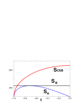
Figure 1: $S_{CEB}$ compared with $S_{H}=(D-2)\frac{HV}{4G_{N}}$ and $S_{B}\equiv 2\pi RE/(D-1)$ in the expanding phase of a closed $D=4$, RD Universe. Here we set $\beta=\frac{D-2}{D-1}$.

A related case is when matter can be modelled by a conformal field theory (CFT). Kutasov and Larsen Kutasov pointed out that for weakly coupled CFT’s in a sphere of radius $R$, the free energy $F$, the entropy $S$ and the total energy $E$ can be expanded at weak coupling and large $x\equiv 2\pi RT$ ,

$$-FR = f(x)=\sum\limits_{n\geq 0}a_{D-2n}x^{D-2n}+\dots\,$$ (28)

$$S = 2\pi f^{\prime}(x)\,,$$ (29)

$$ER = (x\partial_{x}-1)f(x),$$ (30)

where the dots represent non-perturbative contributions.

We can explicitly check under which conditions the entropy of weakly coupled CFT’s obeys the CEB, $S<S_{\rm CEB}=4B\sqrt{\pi}\sqrt{EV}l_{P}^{-(D-2)/2}$. In the limit $TR\gg 1$ we find

$$\frac{S^{2}}{S_{\rm CEB}^{2}}=\frac{\pi a_{D}D^{2}}{4B^{2}(D-1)\Omega_{D-1}}\left(2\pi l_{P}T\right)^{D-2}\,.$$ (31)

Thus, CEB is obeyed provided that

$$\left(\frac{T}{M_{P}}\right)^{D-2}<\frac{K(D)}{a_{D}},$$ (32)

where $K(D)$ is a $D$-dependent (but CFT independent) constant. We conclude that CEB is obeyed as long as temperatures are below $M_{P}$ by a factor $a_{D}^{-\frac{1}{D-2}}$ Since $a_{D}$ is proportional to the number ${\cal N}$ of CFT-matter species, we obtain a bound on temperature which scales as ${\cal N}^{-\frac{1}{D-2}}$ in Planck units.

We can also explicitly check under which conditions strongly coupled CFT’s possessing AdS duals as considered by Verlinde EV obey the CEB. For such CFT’s,

$$S=\frac{c}{12}\frac{V}{L^{D-1}}$$ (33)

$$E=\frac{c}{12}\frac{D-1}{4\pi L}\left(1+\frac{L^{2}}{R^{2}}\right)\frac{V}{L^{D-1}}$$ (34)

$$T=\frac{1}{4\pi L}\left(D+(D-2)\frac{L^{2}}{R^{2}}\right),$$ (35)

where $c$ is the central charge of the CFT and $L\sim 1/T$ is the AdS radius.

In this case, in the limit $R/L\sim TR\gg 1$ we find

$$\frac{S^{2}}{S_{\rm CEB}^{2}}=\frac{1}{4(D-1)B^{2}}\frac{c}{12}\left(\frac{l_{P}}{L}\right)^{D-2}$$ (36)

and thus CEB is obeyed for

$$\frac{1}{4(D-1)B^{2}}\frac{c}{12}\left(\frac{4\pi T}{DM_{P}}\right)^{(D-2)}<1\,.$$ (37)

Since the central charge $c$ is proportional to the number of CFT fields ${\cal N}$, we obtain a bound on temperature which, in Planck units, scales as ${\cal N}^{-\frac{1}{D-2}}$, exactly as previously obtained for the weakly coupled case.

For the case $ER\sim a_{D}$ (which corresponds to $RT\sim 1$) the validity of the CEB guaranteed by a condition similar to eq. (32).

Finally, we would like to show that CEB holds also when $ER\sim 1$. In this case $S_{CEB}\simeq 4B\sqrt{\pi}\sqrt{V/R}l_{P}^{-(D-2)/2}$ scales as $\left(\frac{R}{l_{P}}\right)^{\frac{D-2}{2}}$. The appropriate setup for calculating the entropy in this case is the microcanonical ensemble with the result $S\sim\log a_{D}\sim\log{\cal N}$; thus $S<S_{CEB}$ is guaranteed for a macroscopic Universe as long as

$$\left(\frac{R}{l_{P}}\right)^{\frac{D-2}{2}}>\log{\cal N}\,.$$ (38)

In a quantum theory of gravity we expect the UV cut-off $\Lambda$ to be finite and to represent an upper bound on $T$ (as in the example of superstring theory and its Hagedorn temperature) and a lower bound on R (as in the minimal compactification radius). Thus conditions (32), (37) for the validity of CEB are satisfied as long as $\left(\frac{\Lambda}{M_{P}}\right)^{D-2}<1/{\cal N}$. A bound of the same form was previously proposed in Bek3 and GSL , and independent arguments in support of bounds of this sort have also been put forward in shortest .

III.4.2 The inflationary Universe

The inflationary universe is completely compatible with the CEB. To a certain extent this is a not such an interesting case, because the CEB is comfortably satisfied.

The entropy balance begins for the inflationary Universe after the end of inflation when the energy of the background is converted to matter. This process is historically called reheating and is associated with a large entropy production. In the following we will assume that the reheating process is instantaneously and complete. We will denote by the subscript $RH$ quantities at the instant of reheating.

Since $\dot{H}$ is subleading in this case it follows from eq. (22) that $R_{CC}\sim 1/H$. In this case the CEB and the HEB are similar,

$$S_{CEB}(t_{RH})=l_{P}^{-2}H(t_{RH})a^{3}(t_{RH}).$$ (39)

Assuming that the energy has been completely converted into radiation, the energy density of the radiation is $\rho(t_{RH})=T^{4}_{RH}$. From the $00$ Einstein equation $l_{P}^{-2}H^{2}=\rho$, thus

$$S_{CEB}(t_{RH}) = T^{4}_{RH}\frac{1}{H(t_{RH})}a^{3}(t_{RH})$$

$$= \frac{T_{RH}}{H(t_{RH})}T^{3}_{RH}a^{3}(t_{RH})$$

$$= \frac{T_{RH}}{H(t_{RH})}S(t_{RH}).$$

Here we have used the expression for the radiation entropy $S(t_{RH})=T^{3}_{RH}a^{3}(t_{RH})$. Since from the $00$ Einstein equation $\frac{T_{RH}}{H(t_{RH})}\sim\sqrt{\frac{M_{P}}{H(t_{RH})}}$, and since we expect that the Hubble parameter at reheat be substantially below the Planck temperature we conclude that the CEB is comfortable satisfied.

III.4.3 A Universe near a turning point

Let us consider either a flat or closed universe with some perfect fluid in thermal equilibrium and a constant equation of state $p=\gamma\rho~{},1>\gamma>-1$, and with an additional small negative cosmological constant $\Lambda=-\lambda$. The universe starts out expanding, reaches a maximal size, and then contracts towards a singularity. In this case the matter entropy within a comoving volume is constant in time. But near the point of maximal expansion the apparent horizon and the Hubble length diverge causing violation of the HEB. However, for a fixed comoving volume, $S_{CEB}\sim VR_{CC}^{-1}$, and, since $R_{CC}$ is never larger than some maximal value, the CEB has a chance of doing better.

To see this explicitly let us consider a 4D example. In this case we obtain from eq. (22)

$$R_{CC}^{-2}=\frac{1}{3}{\rm Max}\left[\frac{1}{2}\rho_{0}(1-3\gamma)a^{-3(1+\gamma)}-2\lambda~{},~{}~{}\frac{3}{2}(1+\gamma)\rho_{0}a^{-3(1+\gamma)}\right],$$ (41)

independently of $\kappa$. The initial energy density is $\rho_{0}$ and $a$ is the ratio of the scale factor to its initial value. Since the maximum is larger than each of the expressions in the brackets

$$R_{CC}^{-2}\geq\frac{1}{2}(1+\gamma)\rho_{0}a^{-3(1+\gamma)}.$$ (42)

It follows that in a fixed comoving volume $S_{CEB}$ scales as $\sim a^{3}R_{CC}^{-1}\sim a^{3/2(1-\gamma)}$. Since $\gamma<1$, this means that $S_{CEB}$ grows during the expansion, reaches a maximum at the turning point, and then starts decreasing. If the initial conditions are fixed at at sufficiently early times when curvature and cosmological constant are negligible, the CEB will be obeyed initially provided energy density and curvature are less than Planckian. But then the evolution of $S_{CEB}$ that we have found will guarantee that the bound is satisfied at all times until Planckian density and curvature is reached in the recollapsing phase. Thus the CEB will be satisfied throughout the classical evolution of our Universe.

III.4.4 A static Universe

The simplest example of a non-singular cosmology is a static Einstein model in $D$ dimensions which was discussed in BFM . This model requires positive curvature, and two types of sources: cosmological constant and dust; we denote by $\rho_{\Lambda}$ and $\rho_{\rm m}$ the energy densities associated with each of the two components. To provide entropy we need an additional source, which we choose to be radiation consisting of ${\cal N}$ species in thermal equilibrium at temperature $T$. The energy density of the radiation is given by $\rho_{\rm r}={\cal N}T^{D}$, and the entropy density of the radiation is given by $s_{\rm r}={\cal N}T^{D-1}$ (we ignore here numerical factors since we will be interested in scaling of quantities). The total entropy of the system is given entirely by the entropy of the radiation $S_{\rm r}=s_{\rm r}V$.

In term of these sources, Einstein’s equations can be written in the following way:

$$H^{2}+\frac{1}{a^{2}} = \frac{16\pi G_{\rm N}}{(D-2)(D-1)}\rho_{\rm tot}=\frac{16\pi G_{\rm N}}{(D-2)(D-1)}\left(\rho_{\Lambda}+\rho_{\rm m}+\rho_{\rm r}\right)$$ (43)

$$\dot{H}-\frac{1}{a^{2}} = -\frac{8\pi G_{\rm N}}{(D-2)}\left(\rho_{\rm tot}+p_{\rm tot}\right)$$ (44)

$$= -\frac{8\pi G_{\rm N}}{(D-2)(D-1)}\left[D\rho_{\rm r}+(D-1)\rho_{\rm m}\right]\,,$$

where we have used in eq. (44) the equations of state relating pressure to energy density: $p_{\Lambda}=-\rho_{\Lambda}$, $p_{\rm m}=0$, and $(D-1)p_{\rm r}=\rho_{\rm r}$.

For given $\rho_{\rm m}$ and $\rho_{\rm r}$, one can choose $\rho_{\Lambda}$ and the scale factor $a$ such that $H$ and $\dot{H}$ vanish in eqs. (43) and (44), and thus obtains a static solution. In particular, the condition given by eq. (44) determines the scale factor in terms of $\rho_{\rm m}$ and $\rho_{\rm r}$,

$$a^{2}=\frac{(D-2)(D-1)}{8\pi G_{\rm N}}\frac{1}{D\rho_{\rm r}+(D-1)\rho_{\rm m}}\,.$$ (45)

Since both $H$ and $\dot{H}$ vanish identically, $R_{\rm CC}$ is determined solely by the scale factor $a$ given in eq. (45), as discussed previously.

We now wish to determine under which conditions (if any) some violations of CEB may occur in this model. Recall that according to eq. (20) the CEB bounds the total entropy of a region contained in a comoving volume $V$ by $S_{\rm CEB}=\alpha(D-1)\frac{V}{G_{\rm N}R_{\rm CC}}$, and that in the static case under consideration $R_{\rm CC}=2a/(D-2)$. The square of the ratio of $S_{\rm CEB}$ and the entropy of the system $S_{\rm r}$, is given by

$$\left(\frac{S_{\rm CEB}}{S_{\rm r}}\right)^{2} = \left(\frac{\alpha(D-1)}{s_{\rm r}R_{\rm CC}G_{\rm N}}\right)^{2}$$ (46)

$$= \left[2\pi\alpha^{2}(D-1)(D-2)\right]\left[{D+(D-1){\rho_{\rm m}\over\rho_{\rm r}}}\right]\left[\frac{1}{{\cal N}}\left(\frac{M_{P}}{T}\right)^{D-2}\right].\ \ \ \ \ \ \$$

Since the second factor in expression (46) is larger than unity if $\rho_{\rm m}$ and $\rho_{\rm r}$ are positive, and neglecting the overall prefactor which is independent of the sources in the model, we conclude that the CEB is valid provided that

$${\cal N}\left({T\over M_{\rm P}}\right)^{D-2}\leq 1.$$ (47)

This is the same condition discussed above which should be interpreted as a requirement that temperatures are sub-Planckian, in the case of many number of species ${\cal N}$.

Our conclusion is that as long as the temperature of radiation stays well below Planckian, CEB is upheld. The fact that the model is gravitationally unstable to matter perturbations does not seem to be particularly relevant to the issue of validity of the CEB.

III.4.5 Bekenstein’s non-singular Universe

A time-dependent non-singular cosmological model was found years ago by Bekenstein bmodel (see also mayo ). This is a 4D Friedman-Robertson-Walker universe which is conformal to the closed Einstein Universe. It contains dust, consisting of $N$ particles of mass $\mu$ ($N$ is constant and $\mu$ is positive), coupled to a classical conformal massless scalar field $\psi$, and ${\cal N}$ species of radiation in thermal equilibrium. The action for the dust-$\psi$ system is given by

$${\cal S}=-\frac{1}{2}\int\sqrt{-g}\left[\left(\nabla\psi\right)^{2}+\frac{1}{6}\psi^{2}R\right]d^{4}x-\int\left(\mu+f\psi\right)d\tau.$$ (48)

It includes in addition to the usual action for free point particles of rest mass $\mu$, a dust-scalar field interaction whose strength is determined by the coupling $f$. Accordingly, we may define the effective mass of the dust particles: $\mu_{\rm eff}=\mu+f\psi$.

The total energy density and pressure in Bekenstein’s Universe are given by

$$\rho_{\rm tot}=\rho_{\rm r}+\rho_{\psi}+\rho_{\rm m},\quad p_{\rm tot} = p_{\rm r}+p_{\psi}+p_{\rm m},$$ (49)

where $\{\rho_{\rm r},p_{\rm r}\}$, $\{\rho_{\psi},p_{\psi}\}$, and $\{\rho_{\rm m},p_{\rm m}\}$ are the energy densities and pressures associated with the radiation, scalar field and dust respectively. They depend on the scale factor in the following way

$$\rho_{\rm r} = {\cal C}{\cal N}a^{-4}={\cal N}T^{4},$$

$$\rho_{\psi} = {1\over 2}f^{2}N^{2}a^{-4},$$ (50)

$$\rho_{\rm m} = N\mu_{\rm eff}a^{-3}=N\mu a^{-3}-2\rho_{\psi},$$

and their equations of state $\gamma_{\rm r}=p_{\rm r}/\rho_{\rm r}$, $\gamma_{\psi}=p_{\psi}/\rho_{\psi}$, $\gamma_{\rm m}=p_{\rm m}/\rho_{\rm m}$ are the following

$$\gamma_{\rm r} = 1/3,$$

$$\gamma_{\psi} = -1/3,$$ (51)

$$\gamma_{\rm m} = 0.$$

The dependence of $\psi$ on $a$ $\psi=-fNa^{-1}$, yields $\mu_{\rm eff}=\mu-f^{2}Na^{-1}$. ${\cal C}$ is an integration constant and the only source of entropy is the radiation whose entropy density is given by $s_{\rm r}={\cal N}T^{3}$.

The solution for the scale factor $a$ is given in terms of the conformal time $\eta$ by

$$a(\eta)=a_{0}(1+B\sin\eta).$$ (52)

We assume that $a_{0}$, the mean value of the scale factor, is macroscopic, so it is large in our Planck units. If $B=0$ the solution describes a static universe very similar to the closed Einstein Universe discussed previously. For $0<B<1$ the solution describes a “bouncing universe”: the universe bounces off at $\eta=3\pi/2$ when the scale factor is minimal $a=a_{\rm min}=a_{0}(1-B)$, expands until it turns over at $\eta=5\pi/2$ when its scale factor is maximal $a=a_{\rm max}=a_{0}(1+B)$, and continues to oscillate without ever reaching a singularity. The equations of motion require that the energy densities of the sources obey the following equalities at all times bmodel :

$$2{a\over a_{0}}\left({\rho_{\psi}-\rho_{\rm r}\over 2\rho_{\psi}+\rho_{\rm m}}\right)=1-B^{2}={a_{\rm min}a_{\rm max}\over{a_{0}}^{2}}.$$ (53)

Since $2\rho_{\psi}+\rho_{\rm m}=N\mu a^{-3}>0$, $\rho_{\rm r}>0$, and $B^{2}<1$, it follows that a necessary condition for a bounce is that $\rho_{\rm r}<\rho_{\psi}$. This implies that the total pressure $\frac{1}{3}(\rho_{\rm r}-\rho_{\psi})$ is always negative. Moreover, eq. (53) for $a=a_{\rm min}$ implies that $\rho_{\rm m}\leq-2\rho_{\rm r}<0$ there. But then, the conclusion must be that in order to avoid a singularity, $\mu_{\rm eff}<0$ at least at the bounce. It is possible, however, to find a range of initial conditions and parameters such that $\mu_{\rm eff}$ is positive near the turnover.

The result that $\rho_{\rm r}$ and $\rho_{\psi}$ are manifestly positive definite, but $\rho_{\rm m}$ can (and in fact must) be negative some of the time, suggest that it might be possible to parametrically decrease $\rho_{\rm tot}$ by lowering $\mu_{\rm eff}$ (making it large and negative) by increasing the coupling strength $f$, so that the amounts of radiation and entropy are kept constant. As it turns out this is exactly the case in which the CEB can be potentially violated. Using Einstein’s equations to express $R_{\rm CC}$ in terms of the total energy density and pressure, we find the ratio $\left(S_{\rm CEB}/S_{\rm r}\right)^{2}$:

$$\left({S_{\rm CEB}\over S_{\rm r}}\right)^{2}\sim{G_{\rm N}}^{-2}\left(\frac{\rho_{\rm r}}{\cal N}\right)^{-3/2}\frac{1}{{\cal N}^{2}}G_{\rm N}\,{\rm Max}\left[{\rho_{\rm tot}\over 3}-p_{\rm tot},\rho_{\rm tot}+p_{\rm tot}\right].$$ (54)

A system for which the ratio above is smaller than one would violate the CEB. Recalling that the maximum on the r.h.s. of (54) is always larger than the mean of the two entries and rearranging we find

$$\left({S_{\rm CEB}\over S_{\rm r}}\right)^{2}\geq\left[\frac{1}{{\cal N}}\frac{M_{P}^{2}}{T^{2}}\right]{\rho_{\rm tot}\over\rho_{\rm r}}.$$ (55)

Since we assume that the model is sub-Planckian, namely that the first factor is larger than one as in eq. (47), the only way in which CEB could be violated is if somehow the second factor was parametrically small. As discussed above, it does seem that the second term $\rho_{\rm tot}/\rho_{\rm r}$ can be made arbitrarily small by decreasing $\rho_{\rm tot}$ while keeping $\rho_{\rm r}$ constant. Consequently, it is apparently possible to make the ratio $S_{\rm CEB}/S_{\rm r}$ smaller than one and obtain a CEB violating cosmology. But this can be achieved only if the effective mass of the dust particles is negative (and large) as can be seen from eq. (49).

Violations of the CEB (and as a matter of fact, of any other entropy bound) go hand in hand with large negative energy densities in the dust sector. In the model under discussion, this manifests itself in the form of dust particles with highly negative effective masses. Occurrence of such negative energy density would most probably render the model unstable. We argue that any analysis of entropy bounds should be performed for stable models. This is particularly relevant for the CEB, whose definition involves explicitly the largest scale at which stable BH’s could be formed. However, the instability does not necessarily lead to violations of the CEB as in the previous case. To support this argument we have outlined possible instabilities in the dust scalar field system when the dust particles mass is negative BFM .

III.4.6 The pre-big-bang scenario

Veneziano was the first to study entropy bounds in the context of the PBB scenario HEB . It has been argued GV ; BDV that a form of stochastic PBB is a generic consequence of natural initial conditions corresponding to generic gravitational and dilatonic waves superimposed on the perturbative vacuum of critical superstring theory. In the Einstein-frame metric this can be seen as a chaotic gravitational collapse leading to the formation of BH’s of different sizes. For a string frame observer inside each BH this is viewed as a PBB inflationary cosmology. The duration of the inflationary phase is controlled by the size of the BH GV ; BDV , so from this point of view the observable Universe should be identified with the region of space that was originally inside a sufficiently large BH.

In HEB Veneziano studied a 4D PBB model and followed the evolution of several contributions to the entropy. At time $t=t_{i}$, corresponding to the first appearance of a horizon, he used the Bekenstein–Hawking formula to evaluate that the entropy in the collapsed region $S_{coll}$. Then he used the fact BDV that the initial size of the BH horizon determines the initial value of the Hubble parameter and found that

$$S_{coll}\sim(R_{in}/l_{P,in})^{2}\sim(H_{in}l_{P,in})^{-2}=S_{HEB}.$$ (56)

Thus, initially the entropy is as large as allowed by the HEB (without fine-tuning). Here it was implicitly assumed the initial string coupling is small.

After a short transient phase, dilaton-driven inflation (DDI) should follow GV ; BDV and last until $t_{s}$, the time at which a string-scale curvature is reached. We expect this classical process not to generate further entropy. During DDI $S_{HEB}$ remains constant and the bound continues to be saturated. This follows from the “conservation law” of string cosmology PBBrev

$$\partial_{t}\left(e^{-\phi}\sqrt{g}H\right)=0,$$ (57)

hence

$$\partial_{t}\left((\sqrt{g}H^{3})~{}~{}(e^{-\phi}H^{-2})\right)=\partial_{t}\left(n_{H}S^{H}\right)=0~{}.$$ (58)

Veneziano suggested the following interpretation: At the beginning of the DDI phase the whole entropy is in a single Hubble volume. As DDI proceeds, the same total amount of entropy becomes equally shared between very many Hubble volumes until, eventually, each one of them contributes a small number.

While the coupling is still small $S_{HEB}$ cannot decrease,

$$\partial_{t}(e^{-\phi}\sqrt{g}H)\geq 0.$$ (59)

It follows that

$$(\dot{\phi}-3H)\leq\dot{H}/H\;.$$ (60)

Veneziano noticed that this constraint may be important. As $\alpha^{\prime}$ corrections intervene to stop the growth of $H$, the entropy bound forces $\dot{\phi}-3H$ to decrease and eventually to change sign if $H$ stops growing. But this is just what is needed to convert the DDI solution into the FRW solution PBBrev .

If the initial conditions are such that the string coupling becomes strong while the curvature is still small then Veneziano argued HEB that the HEB forces a non-singular PBB cosmology as well. This time the entropy production by the squeezing of quantum fluctuations is the important factor. This will be discussed further when we discuss the generalized second law.

III.5 Conditions for the validity of the CEB in cosmology

We may summarize the lessons of the previous examples by imposing conditions on sources in a generic cosmological setting such that the CEB is obeyed.

We consider a cosmic fluid consisting of radiation, an optional cosmological constant, and additional unspecified classical dynamical sources which do not include any contributions from the cosmological constant or radiation. For simplicity we assume that the additional sources have negligible entropy. This is the most conservative assumption: if some of the additional sources have substantial entropy our conclusions can be strengthened. We use the previous notations for the total, cosmological, and radiation energy densities, $\rho_{\rm tot}$, $\rho_{\Lambda}$ and $\rho_{\rm r}$ respectively, and denote by $\rho^{*}$ the combined energy density of the additional sources. Thus

$$\rho_{\rm tot}=\rho_{\rm r}+\rho_{\Lambda}+\rho^{*}.$$ (61)

We use the same notation for the relative pressures, and for the equation of state $\gamma^{*}\equiv\rho^{*}/p^{*}$, which may be time-dependent.

In term of these sources, the causal connection scale can be written as

$$R_{\rm CC}^{-2}=\frac{4\pi G_{\rm N}}{D-1}{\rm Max}\Biggl{\{}D\rho_{\Lambda}+\biggl{[}1-(D-1)\gamma^{*}\biggr{]}\rho^{*}\,,$$

$$(D-4)\rho_{\Lambda}+\biggl{[}(2D-5)+(D-1)\gamma^{*}\biggr{]}\rho^{*}+2(D-2)\rho_{\rm r}\Biggr{\}}.$$ (62)

We may now express the ratio of $(S_{\rm CEB}/S_{\rm r})^{2}$, neglecting as usual prefactors of order one

$$\left(\frac{S_{\rm CEB}}{S_{\rm r}}\right)^{2}\sim\frac{1}{{\cal N}}\left(\frac{M_{\rm P}}{T}\right)^{D-2}{\rm Max}\Biggl{\{}D\frac{\rho_{\Lambda}}{\rho_{\rm r}}+\biggl{[}1-(D-1)\gamma^{*}\biggr{]}\frac{\rho^{*}}{\rho_{\rm r}},$$

$$(D-4)\frac{\rho_{\Lambda}}{\rho_{\rm r}}+\biggl{[}(2D-5)+(D-1)\gamma^{*}\biggr{]}\frac{\rho^{*}}{\rho_{\rm r}}+2(D-2)\Biggr{\}}.$$ (63)

Any CEB violations requires that this ratio be parametrically smaller than one. Notice that the first factor is larger than one by our requirement that the radiation energy density be sub-Planckian. Thus the only remaining possibility for violating CEB is that the second factor be parametrically smaller than unity. As we show below, this can occur only if at least one of the additional sources has negative energy density.

The r.h.s. of (63) is larger than the average of the two entries, so that

$$\left(\frac{S_{\rm CEB}}{S_{\rm r}}\right)^{2}\geq{1\over{\cal N}}\left({M_{\rm P}\over T}\right)^{D-2}(D-2){\rho_{\rm tot}\over\rho_{\rm r}}.$$ (64)

Therefore, since $\rho_{\rm tot}>0$, a necessary condition for this expression to be smaller than unity is that $\rho_{\rm tot}\ll\rho_{\rm r}$, which we may reexpress as

$$\frac{\rho_{\Lambda}}{\rho_{\rm r}}\sim-\left(1+\frac{\rho^{*}}{\rho_{\rm r}}\right).$$ (65)

This is not a sufficient condition since the equations of motion could dictate, for example, that the first factor on the r.h.s. of eq. (64) could be parametrically larger than unity at the same time. By substituting condition (65) into eq. (63), we obtain

$$\left(\frac{S_{\rm CEB}}{S_{\rm r}}\right)^{2}\sim\frac{1}{{\cal N}}\left(\frac{M_{\rm P}}{T}\right)^{D-2}\times$$

$${\rm Max}\left\{-\biggl{[}(D-1)(1+\gamma^{*})\frac{\rho^{*}}{\rho_{\rm r}}+D\biggr{]}\,,(D-1)(1+\gamma^{*})\frac{\rho^{*}}{\rho_{\rm r}}+D\right\}.$$ (66)

Therefore, an additional necessary condition for $S_{CEB}/S_{\rm r}$ to be smaller than one is that

$$(1+\gamma^{*})\rho^{*}\simeq-\frac{D}{(D-1)}\rho_{\rm r}\,.$$ (67)

Condition (67) can be satisfied in two ways:

(i) $1+\gamma^{*}>0$ and $\rho^{*}<0$. This obviously requires that at least one of the sources has negative energy density. In this case (barring pathologies) the magnitude of $\rho^{*}$ is comparable to that of $\rho_{\rm r}$.

(ii) $1+\gamma^{*}<0$ and $\rho^{*}>0$. However, for classical dynamical sources, this typically clashes with causality which requires that the pressure and energy density of each of the additional dynamical sources obey $|p_{i}|<|\rho_{i}|$; hence if all $\rho_{i}>0$ then necessarily $\gamma^{*}=\left(\sum p_{i}\right)/\left(\sum\rho_{i}\right)>-1$.

Consequently, condition (67) cannot be satisfied if all of the dynamical sources have positive energy densities and equations of state $|\gamma_{i}|\leq 1$. Bekenstein’s Universe discussed previously fits well within our framework: the total energy density is positive, but the overall contribution to $\rho_{\rm tot}$ of all the sources, excluding radiation (since the cosmological constant vanishes in this case), is negative and almost cancels the contribution of radiation, leaving a small positive $\rho_{\rm tot}$.

To summarize, if all dynamical sources (different from the cosmological constant) have positive energy densities $\rho_{i}>0$ and have causal equations of state ($|\gamma_{i}|\leq 1$), and if radiation temperatures are sub-Planckian, CEB is upheld.

III.6 The CEB and the singularity theorems

The CEB (and entropy bounds in general) refines the classic singularity theorems. It is satisfied by cosmologies for which the singularity theorems are not applicable because some of the energy conditions are violated, but do not seem to be problematic in any of their properties. Conversely, it indicates possible problems when the singularity theorems seem perfectly valid.

In general, the total energy-momentum tensor of a closed “bouncing” universe violates the SEC, but it can obey the CEB. In order to see this explicitly let us consider the “bounce” condition, i.e.  $H=0$, $\dot{H}>0$ for a closed Universe; by using the Einstein equations (43-44), we can express this condition in terms of the sources as follows:

$$\rho_{\rm tot}>0,\quad(D-3)\rho_{\rm tot}+(D-1)p_{\rm tot}<0.$$ (68)

The second of these conditions is (in $D=4$) precisely the condition for violation of the SEC. In terms of $\rho_{\rm r}$, $\rho_{\Lambda}$ and $\rho^{*}$ this reads

$$2\rho_{\Lambda}-(D-2)\rho_{\rm r}-\biggl{[}(D-3)+(D-1)\gamma^{*}\biggr{]}\rho^{*}>0\,.$$ (69)

In comparison, a necessary condition that the CEB is violated can be obtained from eqs.(65) and (67),

$$2\rho_{\Lambda}-(D-2)\rho_{\rm r}-\biggl{[}(D-3)+(D-1)\gamma^{*}\biggr{]}\rho^{*}\sim 0\,,$$ (70)

where the l.h.s of (70) can be either positive or negative. So we find that there is a range of parameters for which the CEB can be obeyed in some bouncing cosmologies but not in others.

In a spatially flat universe ($\kappa=0$), the conditions for a bounce are slightly different: $\rho_{\rm tot}=0$ and $\rho_{\rm tot}+p_{\rm tot}<0$. At the bounce these conditions imply violation of the Null Energy Condition (NEC). As discussed previously, classical sources are not expected to violate the NEC, but effective quantum sources (such as Hawking radiation) are known to violate the NEC. In terms of $\rho_{\rm r}$, $\rho_{\Lambda}$ and $\rho^{*}$ the condition for a bounce reads

$$\left(1+\frac{1}{D-1}\right)\rho_{\rm r}+(1+\gamma^{*})\rho^{*}>0.$$ (71)

In comparison, a necessary condition that the CEB is violated can be obtained from eq. (67),

$$\left(1+\frac{1}{D-1}\right)\rho_{\rm r}+(1+\gamma^{*})\rho^{*}\sim 0\,,$$ (72)

where the l.h.s of (72) can be either positive or negative. So, again, we find that there is a range of parameters for which the CEB can be obeyed in some spatially flat bouncing cosmologies but not in others.

The CEB appears to be a more reliable criterion than energy conditions when trying to decide whether a certain cosmology is reasonable: taking again the closed deSitter Universe as an example, we can add a small amount of radiation to it, and still have a bouncing model if $\rho_{\Lambda}$ is the dominant source, and SEC will not be obeyed (see eq. (69)). Nevertheless, the general discussion in this section shows that in this case the CEB is not violated as long as radiation temperatures remain subPlanckian, despite the presence of a bounce. This happens, in part, because the CEB is able to discriminate better between dynamical and non-dynamical sources (such as the cosmological constant), and imposes constraints that involve the former ones only, such as eq. (67).

We have reached the following conclusions by studying the validity of the CEB for non-singular cosmologies:

1. Violation of the CEB necessarily requires either high temperatures ${\cal N}\left(\frac{T}{M_{\rm P}}\right)^{D-2}\geq 1$, or dynamical sources that have negative energy densities with a large magnitude, or sources with acausal equation of state. Of course, neither of the above is sufficient to guarantee violations of the CEB.

2. Classical sources of this type are suspect of being unphysical or unstable, but each source has to be checked on a case by case basis. In the examples that we have discussed the sources were indeed found to be unstable or are strongly suspected to be so.

3. Sources with large negative energy density could allow, in principle, to increase the entropy within a given volume, while keeping its boundary area and the total energy constant. This would lead to violation of all known entropy bounds, and of any entropy bound which depends in a continuous way on the total energy or on the linear size of the system.

4. The CEB is more discriminating than singularity theorems. In the examples we have considered it allows non-singular cosmologies for which singularity theorems cannot be applied, but does not allow them if they are associated with specific dynamical problems.

III.7 Comparison of the CEB to other entropy bounds

Finally, we compare our CEB to other bounds, in particular to Bekenstein’s and Bousso’s. For systems of limited gravity whose size exceeds their Schwarzschild radius: $R>R_{g}$, Bekenstein’s bound is given by $S<S_{BEB}=l_{P}^{-2}R~{}R_{g}$, and Bousso’s procedure results in the holography bound, $S<S_{HOL}=l_{P}^{-2}R^{2}$, but since $R>R_{g}$, $S_{BEB}<S_{HOL}$, and therefore Bousso’s bound is less stringent than Bekenstein’s. Consider now the CEB applied to the region of size $R$ containing an isolated system. Expressing CEB in the form (8) one immediately obtains: $S_{CEB}=l_{P}^{-1}R^{3/2}E^{1/2}\hbar^{-1/2}=(S_{HOL}~{}~{}S_{BEB})^{1/2}\;,$ implying $S_{BEB}\leq S_{CEB}\leq S_{HOL}.$ We conclude that for isolated systems of limited self-gravity the Bekenstein bound is the tightest, followed by our CEB and, finally, by Bousso’s holographic bound. Similar scaling properties for the HEB were discussed in HEB .

For regions of space that contain so much energy that the corresponding gravitational radius $R_{g}$ exceeds $R$, Bekenstein’s bound is the weakest, while the naive holography bound is the strongest (but very often wrong). Bousso’s proposal uses the apparent horizon $R_{AH}$ while CEB uses $R_{CC}$. For homogeneous cosmologies, $R_{CC}<R_{AH}$, since $R_{CC}^{-2}$, according to (12), is always larger than the average of the two terms appearing on its r.h.s., which is precisely $R_{AH}^{-2}=H^{2}+\kappa/a^{2}$. Since, for a fixed volume, the bounds scale like $R_{AH}^{-1}$ or $R_{CC}^{-1}$, we immediately find that CEB is generally more generous. An important difference between our proposal and Bousso’s covariant holographic bound boussorev that scales as $S/A$ is that there the entropy $S$ is a flux through light-like hypersurfaces. A detailed comparison with Bousso’s proposal is therefore more subtle because of his use of the apparent horizon area to bound entropy on light sheets. This can be converted into a bound on the entropy of the space-like region only in special cases.

E. Verlinde EV argued that the radiation in a closed, radiation dominated Universe can be modelled by a CFT, and that its entropy can be evaluated using a generalized Cardy formula. After an appropriate modification of Verlinde’s bound which evades the criticism about its validity for weakly coupled CFT’s the new bound is exactly equivalent to CEB within the CFT framework.

IV The Generalized second law and the Causal Entropy Bound

IV.0.1 The Generalized second law in Cosmology

There seems to be a close relationship between entropy bounds and the GSL. We have proposed a concrete classical and quantum mechanical form of the GSL in cosmology GSL , which is valid also in situations far from thermal equilibrium. We discuss various entropy sources, such as thermal, “geometric” and “quantum” entropy, apply GSL to study cosmological solutions, and show that it is compatible with entropy bounds. GSL allows a more detailed description of how, and if, cosmological singularities are evaded. The proposed GSL is different from GSL for BH’s gslbh , but the idea that in addition to normal entropy other sources of entropy have to be included has some similarities. We will discuss here only 4D models. Obviously it should be possible to generalize our analysis to higher dimensions in a straightforward manner along the lines of the generalizations of the CEB to higher dimensions.

The starting point of our classical discussion is the definition of the total entropy of a domain containing more than one cosmological horizon HEB . We have already introduced the number of cosmological horizons within a given comoving volume $V=a(t)^{3}$. It is simply the total volume divided by the volume of a single horizon, $n_{H}={a(t)^{3}}/{|H(t)|^{-3}}$. As usual we will ignore numerical factors of order unity. Here we use units in which $c=1,G_{N}=1/16\pi,\hbar=1$ and discuss only flat, homogeneous, and isotropic cosmologies. If the entropy within a given horizon is $S^{H}$, then the total entropy is given by $S=n_{H}S^{H}$. Classical GSL requires that the cosmological evolution, even when far from thermal equilibrium, must obey $dS\geq 0,$ in addition to Einstein’s equations. In particular,

$$n_{H}\partial_{t}S^{H}+\partial_{t}n_{H}S^{H}\geq 0.$$ (73)

In general, there could be many sources and types of entropy, and the total entropy is the sum of their contributions. If, in some epoch, a single type of entropy makes a dominant contribution to $S^{H}$, for example, of the form $S^{H}=|H|^{\alpha}$, $\alpha$ being a constant characterizing the type of entropy source, and therefore $S=(a|H|)^{3}|H|^{\alpha}$, eq. (73) becomes an explicit inequality,

$$3H+(3+\alpha)\frac{{\dot{H}}}{H}\geq 0,$$ (74)

which can be translated into energy conditions constraining the energy density $\rho$, and the pressure $p$ of (effective) sources. Using the FRW equations,

$$H^{2} = \ \frac{1}{6}\ \rho$$

$${\dot{H}} = -\frac{1}{4}(\rho+p)$$ (75)

$${\dot{\rho}} + 3H(\rho+p)=0,$$

and assuming $\alpha>-3$ (which we will see later is a reasonable assumption ) and of course $\rho>0$, we obtain

$$\frac{p}{\rho} \leq \frac{2}{3+\alpha}-1\hskip 18.06749pt\hbox{for}\hskip 18.06749ptH>0,$$ (76)

$$\frac{p}{\rho} \geq \frac{2}{3+\alpha}-1\hskip 18.06749pt\hbox{for}\hskip 18.06749ptH<0.$$ (77)

Adiabatic evolution occurs when the inequalities in eqs.(76,77) are saturated.

A few remarks about the allowed range of values of $\alpha$ are in order. First, the usual adiabatic expansion of a radiation dominated universe with $p/\rho=1/3$ corresponds to $\alpha=-3/2$. Adiabatic evolution with $p/\rho<-1$, for which the null energy condition is violated would require a source for which $\alpha<-3$. This is problematic since it does not allow a flat space limit of vanishing $H$ with finite entropy. The existence of an entropy source with $\alpha$ in the range $\alpha<-2$ does not allow a finite $\partial_{t}S$ in the flat space limit and is therefore suspected of being unphysical. Finally, the equation of state $p=-\rho$ (deSitter inflation), cannot be described as adiabatic evolution for any finite $\alpha$.

Let us discuss in more detail three specific examples. First, as already noted, we have verified that thermal entropy during radiation dominated (RD) evolution can be described without difficulties, as expected. In this case, $\alpha=-\frac{3}{2}$, reproduces the well known adiabatic expansion, but also allows entropy production. The present era of matter domination requires a more complicated description since in this case one source provides the entropy, and another source the energy.

The second case is that of geometric entropy $S_{g}$, whose source is the existence of a cosmological horizon gibbons ; Srednicki:1993im . The concept of geometric entropy is closely related to the holographic principle and to entanglement entropy (see below). For a system with a cosmological horizon $S^{H}_{g}$ is given by (ignoring numerical factors of order unity)

$$S_{g}^{H}=|H|^{-2}G_{N}^{-1}.$$ (78)

The equation of state corresponding to adiabatic evolution with dominant $S_{g}$, is obtained by substituting $\alpha=-2$ into eqs.(76,77), leading to $p/\rho=1$ for positive and negative $H$. This equation of state is simply that of a free massless scalar field, also recognized as the two vacuum branches of PBB string cosmology PBBrev in the Einstein frame. In HEB this was found for the $(+)$ branch in the string frame as an “empirical” observation. In general, for the case of dominant geometric entropy, GSL requires, for positive $H$, $p\leq\rho,$ hence deSitter inflation is definitely allowed. For negative $H$, GSL requires $\rho\leq p,$ and therefore forbids, for example, a time reversed history of our universe or a contracting deSitter universe with a negative constant $H$ (unless some additional entropy sources appear).

The third case is that of quantum entropy $S_{q}$, associated with quantum fluctuations. This form of entropy was discussed in BMP ; gg . Specific quantum entropy for a single physical degree of freedom is approximately given by (again, ignoring numerical factors of order unity)

$$s_{q}=\int d^{3}k\ln n_{k},$$ (79)

where $n_{k}\gg 1$ are occupation numbers of quantum modes. Quantum entropy is large for highly excited quantum states, such as the squeezed states obtained by amplification of quantum fluctuations during inflation. Quantum entropy does not seem to be expressible in general as $S^{H}_{q}=|H|^{\alpha}$, since occupation numbers depend on the whole history of the evolution. We will discuss this form of entropy in more detail later, when the quantum version of GSL is proposed.

Geometric entropy is related to the existence of a horizon or more generally to the existence of a causal boundary. From my current perspective the geometric entropy corresponds to entanglement entropy of fluctuations whose wavelength is shorter than the horizon while “quantum” entropy is probably related to entanglement entropy of fluctuations whose wavelength is larger than the horizon (see below).

We would like to show that it is possible to formally define a temperature, and that the definition is compatible with the a generalized form of the first law of thermodynamics (see also Jacobson ). Recall that the first law for a closed system states that $TdS=dE+pdV=(\rho+p)dV+Vd\rho.$ Let us now consider the case of single entropy source and formally define a temperature $T$, $T^{-1}=\left(\frac{\partial S}{\partial E}\right)_{V}=\frac{\partial s}{\partial\rho},$ since $E=\rho V$ and $S=sV$. Using eqs.(75), and $s=|H|^{\alpha+3}$, we obtain $\frac{\partial s}{\partial\rho}=\frac{\alpha+3}{12}|H|^{\alpha+1},$ and therefore

$$T=\frac{12}{\alpha+3}|H|^{-\alpha-1}.$$ (80)

To ensure positive temperatures $\alpha>-3,$ a condition which we have already encountered. Additionally, for $\alpha>-1$, $T$ diverges in the flat space limit, and therefore such a source is suspect of being unphysical, leading to the conclusion that the physical range of $\alpha$ is $-2\leq\alpha\leq-1$. A compatibility check requires $T^{-1}=\frac{\partial s}{\partial t}/\frac{\partial\rho}{\partial t}$, which indeed yields a result in agreement with (80). Yet another thermodynamic relation $p/T=\left(\frac{\partial S}{\partial V}\right)_{E}$, leads to $p=sT-\rho$ and therefore to $p/\rho=\frac{2}{\alpha+3}-1$ for adiabatic evolution, in complete agreement with eqs.(76,77). For $\alpha=-2$, eq. (80) implies $T_{g}=|H|$, in agreement with gibbons , and for ordinary thermal entropy $\alpha=-3/2$ reproduces the known result, $T=|H|^{1/2}$.

Is GSL compatible with entropy bounds? Let us start answering this question by considering a universe undergoing decelerated expansion, that is $H>0$, $\dot{H}<0$. For entropy sources with $\alpha>-2$, going backwards in time, $H$ is prevented by the restriction $S^{H}\leq S_{g}^{H}$ from becoming too large. This requires that at a certain moment in time $\dot{H}$ has reversed sign, or at least vanished. GSL allows such a transition. Evolving from the past towards the future, and looking at eq. (74) we see that a transition from an epoch of accelerated expansion $H>0$, $\dot{H}>0$, to an epoch of decelerated expansion $H>0$, $\dot{H}<0$, can occur without violation of GSL. But later we discuss a new bound appearing in this situation when quantum effects are included.

For a contracting Universe with $H<0$, and if sources with $\alpha>-2$ exist, the situation is more interesting. Let us check whether in an epoch of accelerated contraction $H<0$, $\dot{H}<0$, GSL is compatible with entropy bounds. If an epoch of accelerated contraction lasts, it will inevitably run into a future singularity, in conflict with bound $S^{H}\leq S_{g}^{H}$. This conflict could perhaps have been prevented if at some moment in time the evolution had turned into decelerated contraction with $H<0$, $\dot{H}>0$. But a brief look at eq. (74), $\dot{H}\leq-\frac{3}{3+\alpha}H^{2}$, shows that decelerated contraction is not allowed by GSL. The conclusion is that for the case of accelerated contraction GSL and the entropy bound are not compatible.

To resolve the conflict between GSL and the entropy bound, we propose adding a missing quantum entropy term $dS_{Quantum}=-\mu dn_{H},$ where $\mu(a,H,\dot{H},...)$ is a “chemical potential” motivated by the following heuristic argument. Specific quantum entropy is given by (79), and we consider for the moment one type of quantum fluctuations that preserves its identity throughout the evolution. Changes in $S_{q}$ result from the well known phenomenon of freezing and defreezing of quantum fluctuations. For example, quantum modes whose wavelength is stretched by an accelerated cosmic expansion to the point that it is larger than the horizon, become frozen (“exit the horizon”), and are lost as dynamical modes, and conversely quantum modes whose wavelength shrinks during a period of decelerated expansion (“reenter the horizon”), thaw and become dynamical again. Taking into account this “quantum leakage” of entropy, requires that the first law should be modified as in open systems $TdS=dE+PdV-\mu dN$.

Consider a universe going through a period of decelerated expansion, containing some quantum fluctuations which have reentered the horizon (for concreteness, it is possible to think about an isotropic background of gravitational waves). In this case, physical momenta simply redshift, but since no new modes have reentered, and since occupation numbers do not change by simple redshift, then within a fixed comoving volume, entropy does not change. However, if there are some frozen fluctuations outside the horizon “waiting to reenter” then there will be a change in quantum entropy, because the minimal comoving wave number of dynamical modes $k_{min}$, will decrease due to the expansion, $k_{min}(t+\delta t)<k_{min}(t)$. The resulting change in quantum entropy, for a single physical degree of freedom, is $\Delta s_{q}=\!\!\!\int\limits_{k_{min}(t+\delta t)}^{k_{min}(t)}\!\!\!k^{2}dk\ln n_{k},$ and since $k_{min}(t)=a(t)H(t)$, $\Delta S_{q}=\!\!\!\int\limits_{a(t+\delta t)H(t+\delta t)}^{a(t)H(t)}k^{2}dk\ln n_{k}=-\Delta(aH)^{3}\ln n_{k=aH},$ provided $\ln n_{k}$ is a smooth enough function. Therefore, for ${\cal N}$ physical DOF, and since $n_{H}=(aH)^{3}$,

$$dS_{q}=-\mu{\cal N}dn_{H},$$ (81)

where parameter $\mu$ is taken to be positive. Obviously, the result depends on the spectrum $n_{k}$, but typical spectra are of the form $n_{k}\sim k^{\beta}$, and therefore we may take as a reasonable approximation $\ln n_{k}\sim constant$ for all ${\cal N}$ physical DOF.

We adopt proposal (81) in general,

$$dS = dS_{Classical}+dS_{Quantum}$$ (82)

$$= dn_{H}S^{H}+n_{H}dS^{H}-\mu{\cal N}dn_{H},$$

where $S^{H}$ is the classical entropy within a cosmological horizon. In particular, for the case that $S^{H}$ is dominated by a single source $S^{H}=|H|^{\alpha}$,

$$\left(3H+3\frac{{\dot{H}}}{H}\right)n_{H}(S^{H}-\mu{\cal N})+\alpha\frac{{\dot{H}}}{H}n_{H}S^{H}\geq 0.$$ (83)

Quantum modified GSL (83) allows a transition from accelerated to decelerated contraction. As a check, look at $H<0$, $\dot{H}=0$, in this case modified GSL requires $3H(S^{H}-\mu{\cal N})\geq 0,$ which, if $\mu{\cal N}\geq S^{H}$, is allowed. If the dominant form of entropy is indeed geometric entropy, the transition from accelerated to decelerated contraction is allowed already at $|H|\sim M_{P}/\sqrt{{\cal N}}$. In models where ${\cal N}$ is a large number, such as grand unified theories and string theory where it is expected to be of the order of 1000, the transition can occur at a scale much below the Planck scale, at which classical general relativity is conventionally expected to adequately describe background evolution.

If we reconsider the transition from accelerated to decelerated expansion and require that (83) holds, we discover a new bound derived directly from GSL. It is compatible with, but not relying on, the bound $S^{H}\leq S_{g}^{H}$. Consider the case in which $\dot{H}$ and $H$ are positive, or $H$ positive and $\dot{H}$ negative but $|\dot{H}|\ll H^{2}$, relevant to whether the transition is allowed by GSL. In this case, (83) reduces to $S^{H}-\mu{\cal N}\geq 0$, that is, GSL puts a lower bound on the classical entropy within the horizon. If geometric entropy is the dominant source of entropy as expected, GSL puts a lower bound on geometric entropy $S_{g}^{H}\geq\mu{\cal N}$, which yields an upper bound on $H$,

$$H\leq\frac{M_{P}}{\sqrt{{\cal N}}}.$$ (84)

The scale that appeared previously in the resolution of the conflict between entropy bounds and GSL for a contracting universe has reappeared in (84), and remarkably, (84) is the same bound obtained in Bek3 using different arguments. Bound (84) forbids a large class of singular homogeneous, isotropic, spatially flat cosmologies by bounding the scale of curvature for a such a universe.

IV.1 The Generalized Second Law in Pre-Big-Bang string cosmology

String theory is a consistent theory of quantum gravity, with the power to describe high curvature regions of space-time Polchinski , and as such we could expect it to teach us about the fate of cosmological singularities, with the expectation that singularities are smoothed and turned into brief epochs of high curvature. However, many attempts to seduce an answer out of string theory regarding cosmological singularities have failed so far in producing a conclusive answer (see for example stringsing ). The reason is probably that most technical advancements in string theory rely heavily on supersymmetry, but generic time dependent solutions break all supersymmetries and therefore known methods are less powerful when applied to cosmology.

We have focused GSLstring on the two sources of entropy defined previously. The first source is the geometric entropy $S_{g}$, and the second source is quantum entropy $S_{q}$. The entropy within a given horizon is $S^{H}$ and the total entropy is given by $S=n_{H}S^{H}$. We will ignore numerical factors, use units in which $c=1$, $\hbar=1$, $G_{N}=e^{\phi}/16\pi$, $\phi$ being the dilaton, and discuss only flat, homogeneous, and isotropic 4D string cosmologies in the so-called string frame, in which the lowest order effective action is ${\cal S}_{\rm LO}=\int d^{4}x\sqrt{-g}e^{-\phi}\left[R+\left(\partial\phi\right)^{2}\right]$. Obviously the discussion can be generalized in a straight forward manner to higher $D$.

In ordinary cosmology, geometric entropy within a Hubble volume is given by its area $S_{g}^{H}=H^{-2}G_{N}^{-1}$, and therefore specific geometric entropy is given by $s_{g}=|H|G_{N}^{-1}$ GSL . A possible expression for specific geometric entropy in string cosmology is obtained by substituting $G_{N}=e^{\phi}$, leading to

$$s_{g}=|H|e^{-\phi}.$$ (85)

Reassurance that $s_{g}$ is indeed given by (85) is provided by the following observation. The action ${\cal S}_{\rm LO}$ can be expressed in a $(3+1)$ covariant form, using the 3-metric $g_{ij}$, the extrinsic curvature $K_{ij}$, considering only vanishing $3-$Ricci scalar and homogeneous dilaton, ${\cal S}_{\rm LO}=\int d^{3}xdt\sqrt{g_{ij}}e^{-\phi}\left[-3K_{ij}K^{ij}-2g^{ij}\partial_{t}{K_{ij}}+K^{2}-(\partial_{t}{\phi})^{2}\right].$ Now, ${\cal S}_{\rm LO}$ is invariant under the symmetry transformation $g_{ij}\rightarrow e^{2\lambda}g_{ij}$, $\phi\rightarrow\phi+3\lambda$, for an arbitrary time dependent $\lambda$. From the variation of the action $\delta{\cal S}=\int d^{3}xdt\sqrt{g_{ij}}e^{-\phi}4K\dot{\lambda}$, we may read off the current and conserved charge $Q=4a^{3}e^{-\phi}K$. The symmetry is exact in the flat homogeneous case, and it seems plausible that it is a good symmetry even when $\alpha^{\prime}$ corrections are present Gasperini:1997fu . With definition (85), the total geometric entropy $S_{g}=a^{3}|H|e^{-\phi},$ is proportional to the corresponding conserved charge. Adiabatic evolution, determined by $\partial_{t}S_{g}=0$, leads to a familiar equation, $\frac{\dot{H}}{H}-\dot{\phi}+3H=0,$ satisfied by the $(\pm)$ vacuum branches of PBB string cosmology.

Quantum entropy for a single field in string cosmology is, as in BMP ; gg ; GSL , given by

$$s_{q}=\int_{k_{min}}^{k_{max}}d^{3}kf(k)\,,$$ (86)

where for large occupation numbers $f(k)\simeq\ln n_{k}$. The ultraviolet cutoff $k_{max}$ is assumed to remain constant at the string scale. The infrared cutoff $k_{min}$ is determined by the perturbation equation $\psi_{k_{c}}^{\prime\prime}+\left(k_{c}^{2}-\frac{\sqrt{s(\eta)}^{\prime\prime}}{\sqrt{s(\eta)}}\right)\psi_{k_{c}}=0,$ where $\eta$ is conformal time ${}^{\prime}=\partial_{\eta}$, and $k_{c}$ is the comoving momentum related to physical momentum $k(\eta)$ as $k_{c}=a(\eta)k(\eta)$. Modes for which $k_{c}^{2}\leq\frac{\sqrt{s}^{\prime\prime}}{\sqrt{s}}$ are “frozen”, and are lost as dynamical modes. The “pump field” $s(\eta)=a^{2m}e^{\ell\phi}$, depends on the background evolution and on the spin and dilaton coupling of various fields. We are interested in solutions for which $a^{\prime}/a\sim\phi^{\prime}\sim 1/\eta$, and therefore, for all particles $\frac{\sqrt{s}^{\prime\prime}}{\sqrt{s}}\sim 1/\eta^{2}$. It follows that $k_{min}\sim H$. In other phases of cosmological evolution our assumption does not necessarily hold, but in standard radiation domination (RD) with frozen dilaton all modes reenter the horizon. Using the reasonable approximation $f(k)\sim$ constant, we obtain, as in GSL ,

$$\Delta S_{q}\simeq-\mu\Delta n_{H}.$$ (87)

Parameter $\mu$ is positive, and in many cases proportional to the number of species of particles, taking into account all DOF of the system, perturbative and non-perturbative. The main contribution to $\mu$ comes from light DOF and therefore if some non-perturbative objects, such as D branes become light they will make a substantial contribution to $\mu$.

We now turn to the generalized second law of thermodynamics, taking into account geometric and quantum entropy. Enforcing $dS\geq 0$, and in particular, $\partial_{t}S=\partial_{t}S_{g}+\partial_{t}S_{q}\geq 0$, leads to an important inequality,

$$\left(H^{-2}e^{-\phi}-\mu\right)\partial_{t}n_{H}+n_{H}\partial_{t}\left(H^{-2}e^{-\phi}\right)\geq 0.$$ (88)

When quantum entropy is negligible compared to geometric entropy, GSL (88) leads to

$$\dot{\phi}\leq\frac{\dot{H}}{H}+3H,$$ (89)

yielding a bound on $\dot{\phi}$, and therefore on dilaton kinetic energy, for a given $H$, $\dot{H}$. Bound (89) was first obtained in HEB , and interpreted as following from a saturated HEB.

When quantum entropy becomes relevant we obtain another bound. We are interested in a situation in which the universe expands, $H>0$, and $\phi$ and $H$ are non-decreasing, and therefore $\partial_{t}\left(H^{-2}e^{-\phi}\right)\leq 0$ and $\partial_{t}n_{H}>0$. A necessary condition for GSL to hold is that

$$H^{2}\leq\frac{e^{-\phi}}{\mu},$$ (90)

bounding total geometric entropy $He^{-\phi}\leq\frac{e^{-\frac{3}{2}\phi}}{\sqrt{\mu}}$. A bound similar to (90) was obtained in HEB by considering entropy of reentering quantum fluctuations. We stress that to be useful in analysis of cosmological singularities (90) has to be considered for perturbations that exit the horizon. If the condition (90) is satisfied then the cosmological evolution always allows a self-consistent description using the low energy effective action approach.

It is not apriori clear that the form of GSL and entropy sources remains unchanged when curvature becomes large, in fact, we may expect higher order corrections to appear. For example, the conserved charge of the scaling symmetry of the action will depend in general on higher order curvature corrections. Nevertheless, in the following we will assume that specific geometric entropy is given by eq. (85), without higher order corrections, and try to verify that, for some reason yet to be understood, there are no higher order corrections to eq. (85). Our results are consistent with this assumption.

We turn now to apply our general analysis to the PBB string cosmology scenario, in which the universe starts from a state of very small curvature and string coupling and then undergoes a long phase of dilaton-driven inflation (DDI), joining smoothly at later times standard RD cosmology, giving rise to a singularity free inflationary cosmology. The high curvature phase joining DDI and RD phases is identified with the ‘big bang’ of standard cosmology. A key issue confronting this scenario is whether, and under what conditions, can the graceful exit transition from DDI to RD be completed Brustein:1994kw . In particular, it was argued that curvature is bounded by an algebraic fixed point behaviour when both $H$ and $\dot{\phi}$ are constants and the universe is in a linear-dilaton deSitter space Gasperini:1997fu , and coupling is bounded by quantum corrections Brustein:1997ny ; Foffa:1999dv . But it became clear that another general theoretical ingredient is missing, and we propose that GSL is that missing ingredient.

We have studied numerically examples of PBB string cosmologies to verify that the overall picture we suggest is valid in cases that can be analyzed explicitly. We first consider, as in Gasperini:1997fu ; Brustein:1999yq , $\alpha^{\prime}$ corrections to the lowest order string effective action,

$${\cal S}=\frac{1}{16\pi\alpha^{\prime}}\int d^{4}x\sqrt{-g}e^{-\phi}\left[R+\left(\partial\phi\right)^{2}+\frac{1}{2}{\cal L}_{\alpha^{\prime}}\right]\,,$$ (91)

where

$${\cal L}_{\alpha^{\prime}}=k\alpha^{\prime}\Biggl{[} \frac{1}{2}R^{2}_{GB}+A\left(\partial\phi\right)^{4}+D\partial^{2}\phi\left(\partial\phi\right)^{2}$$ (92)

$$+C\left(R^{\mu\nu}-\frac{1}{2}g^{\mu\nu}R\right)\partial_{\mu}\phi\partial_{\nu}\phi\Biggr{]},$$

with $C=-(2A+2D+1)$, is the most general form of four derivative corrections that lead to equations of motion with at most second (time) derivatives. The rationale for this choice was explained in Brustein:1999yq . $k$ is a numerical factor depending on the type of string theory. Action (91) leads to equations of motion, $-3H^{2}+\dot{\bar{\phi}}^{2}-\bar{\rho}=0$, $\bar{\sigma}-2\dot{H}+2H\dot{\bar{\phi}}=0$, $\bar{\lambda}-3H^{2}-\dot{\bar{\phi}}^{2}+2\ddot{\bar{\phi}}=0$, where $\bar{\rho}$, $\bar{\lambda}$, $\bar{\sigma}$ are effective sources parameterizing the contribution of $\alpha^{\prime}$ corrections Brustein:1999yq . Parameters $A$ and $D$ should have been determined by string theory, however, at the moment, it is not possible to calculate them in general. If $A$, $D$ were determined we could just use the results and check whether their generic cosmological solutions are non-singular, but since $A$, $D$ are unavailable at the moment, we turn to GSL to restrict them.

First, we look at the initial stages of the evolution when the string coupling and $H$ are very small. We find that not all the values of the parameters $A$, $D$ are allowed by GSL. The condition $\bar{\sigma}\geq 0$, which is equivalent to GSL on generic solutions at the very early stage of the evolution, if the only relevant form of entropy is geometric entropy, leads to the following condition on $A$, $D$ (first obtained by R. Madden dick ), $40.05A+28.86D\leq 7.253.$ The values of $A$, $D$ which satisfy this inequality are labeled “allowed”, and the rest are “forbidden”. In Brustein:1999yq a condition that $\alpha^{\prime}$ corrections are such that solutions start to turn towards a fixed point at the very early stages of their evolution was found $61.1768A+40.8475D\leq 16.083$, and such solutions were labeled “turning the right way”. Both conditions are displayed in Fig. 2. They select almost the same region of $(A,D)$ space, a gratifying result, GSL “forbids” actions whose generic solutions are singular and do not reach a fixed point.

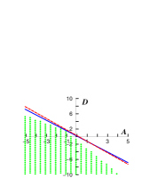
Figure 2: Two lines, separating actions whose generic solutions “turn the right way” at the early stages of evolution (red-dashed), and actions whose generic solutions satisfy classical GSL while close to the $(+)$ branch vacuum (blue-solid). The dots represent $(A,D)$ values whose generic solutions reach a fixed point, and are all in the ”allowed” region.

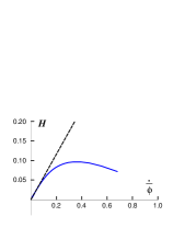
Figure 3: Typical solution that “turns the wrong way”. The dashed line is the $(+)$ branch vacuum.

We further observe that generic solutions which “turn the wrong way” at the early stages of their evolution continue their course in a way similar to the solution presented in Fig. 3. We find numerically that at a certain moment in time $H$ starts to decrease, at that point $\dot{H}=0$ and particle production effects are still extremely weak, and therefore (89) is the relevant bound, but (89) is certainly violated.

We have scanned the $(A,D)$ plane to check whether a generic solution that reaches a fixed point respects GSL throughout the whole evolution, and conversely, whether a generic solution obeying GSL evolves towards a fixed point. The results are shown in Fig. 2, clearly, the “forbidden” region does not contain actions whose generic solutions go to fixed points. Nevertheless, there are some $(A,D)$ values located in the small wedges near the bounding lines, for which the corresponding solutions always satisfy (89), but do not reach a fixed point, and are singular. This happens because they meet a cusp singularity. Consistency requires adding higher order $\alpha^{\prime}$ corrections when cusp singularities are approached, which we will not attempt here.

If particle production effects are strong, the quantum part of GSL adds bound (90), which adds another “forbidden” region in the $(H,\dot{\bar{\phi}})$ plane, the region above a straight line parallel to the $\dot{\bar{\phi}}$ axis. The quantum part of GSL has therefore a significant impact on corrections to the effective action. On a fixed point $\phi$ is still increasing, and therefore the bounding line described by (90) is moving downwards, and when the critical line moves below the fixed point, GSL is violated. This means that when a certain critical value of the coupling $e^{\phi}$ is reached, the solution can no longer stay on the fixed point, and it must move away towards an exit. One way this can happen is if quantum corrections, perhaps of the type discussed in Brustein:1997ny ; Foffa:1999dv exist.

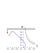
Figure 4: Graceful exit enforced by GSL on generic solutions. The horizontal line is bound (90) and the curve on the right is bound (89), shaded regions indicate GSL violation.

The full GSL therefore forces actions to have generic solutions that are non-singular, classical GSL bounds dilaton kinetic energy and quantum GSL bounds $H$ and therefore, at a certain moment of the evolution $\dot{H}$ must vanish (at least asymptotically), and then curvature is bounded. If cusp singularities are removed by adding higher order corrections, as might be expected, we can apply GSL with similar conclusions also in this case. A schematic graceful exit enforced by GSL is shown in Fig. 4. Our result indicate that if we impose GSL in addition to equations of motion then non-singular PBB string cosmology is quite generic.

V Area entropy, entanglement entropy and entropy bounds

Classical General Relativity predicts space-times with event horizons and other causal boundaries, such as apparent horizons, cosmological horizons and acceleration horizons. Observers in space-times with causal boundaries can see very different physics, as demonstrated by comparing the static observer at infinity and a freely falling observer in the Schwarzchild geometry. For the first, the horizon is a very special place: energies of particles diverge and space-time seems to end there, while for a freely falling observer the horizon and its vicinity do not look special at all. In cosmological space-times with causal boundaries the situation is similar. The existence of causal boundaries is determined by the large scale properties of space-time, and hence is intrinsically a non-local concept. In cosmology, for example, it is hard for a local observer to determine whether the space-time is de Sitter space that has a cosmological event horizon, or a Robertson-Walker space which looks approximately de Sitter.

The interpretation of the thermodynamic properties of BH’s and whether they originate from some underlying, more fundamental, statistical mechanics remains unclear, in spite of the intense efforts and the progress that has been achieved over the last 30 years since the discovery by Bekenstein gslbh . Quantum field theory (QFT) in the fixed background of space-times with horizons is a key element in the quantitative understanding of the statistical mechanics of BH’s. QFT in such background has several interesting and well-known features. The quantum vacuum states associated with different observers can be very different from each other, leading to strong particle production effects: the Hawking effect and the Unruh effect. In addition, the appearance of large blue shifts of quantum modes near the horizon lead to the trans-planckian problem Jacobson:2003vx . The proposed resolutions include the brick-wall model 'tHooft:1984re ; 'tHooft:1996tq and the stretched-horizon Susskind:1993if idea. The entropy and thermodynamics are also observer dependent, as demonstrated by the classic comparison between the Rindler and Minkowski space observers in the Minkowski vacuum. The accelerated observer sees a truly thermal state, while for the Minkowski observer the temperature vanishes. The tension between the possibility of evaluating the entropy and other thermodynamic quantities in the semiclassical approximation and their observer dependence and hence their sensitivity to physics at the highest energy scales is intriguing and is not yet resolved.

My current point of view about the physics of space-times with causal boundaries is the entanglement point of view. I believe that the statistical properties of such space-times arise because classical observers in them have access only to a part of the whole quantum state. When a system is in a pure state, but one cannot access the complete quantum system, and a measurement is performed, one is instructed by the rules of quantum mechanics to trace over the classically inaccessible DOF. This leads to a natural framework for interpreting the physics of spaces with causal boundaries: that it is described by the density matrix which results from tracing over the inaccessible DOF. In the context of BH’s the idea was first proposed by ’t Hooft 'tHooft:1996tq , and by Sorkin and collaborators Bombelli:1986rw , and then extended and elaborated by Srednicki Srednicki:1993im and others.

The entanglement approach considers the fundamental physical objects describing the physics of space-times with causal boundaries to be their global quantum state and the unitary evolution operator. The entanglement approach has several obvious advantages: it leads naturally to area-law entropy, it can incorporate the observer dependence of BH thermodynamics and of the thermodynamics of cosmological space-times with causal boundaries. It can naturally accommodate the geometric and quantum entropies. The first resulting from the entanglement entropy of short wavelength fluctuations and the second resulting from the entanglement entropy of fluctuations whose wavelength is larger than the causal connection scale. This interpretation is also automatically compatible with entropy bounds and the GSL as long as the evolution equations are “physical” because from a global point of view it is clear that nothing special occurs when a horizon develops. Obviously, there are also some unresolved issues that need to be understood better in this context.

The space-times that are traditionally used to explore the entanglement point of view are spaces with bifurcating Killing horizons such as the eternal Schwarzschild BH or Rindler space. Israel Israel:1976ur has shown that the quantum Hilbert space of fields in space-times with bifurcating Killing horizons has a product structure that is isomorphic to the product structure that arises in thermofield dynamics Takahasi:1974zn . In thermofield dynamics one formally doubles the Hilbert space and evaluates quantum expectation values in the thermofield double pure state in order to evaluate expectation values in a thermal state of the original system. In this context the entropy is the entanglement entropy that is obtained from tracing over one of the two spaces.

One of the main unresolved issues confronting the entanglement interpretation is the ultraviolet (UV) divergence of entanglement entropy and other entanglement correlation functions near the horizon, and its dependence on the number of fields Wald:1999vt ; Marolf:2003bb ; Marolf:2004et . Another issue concerns space-times that do not have non-degenerate bifurcating Killing horizons. For such spaces, it is unclear what is entangled with what, since some of the regions of the extended space-time are missing.

The entanglement point of view has been discussed in the AdS-CFT context by Maldacena Maldacena:2001kr who studied eternal BH’s in AdS. In 4D, the space has two boundaries that are topologically $S^{2}\times S^{1}$, the dual FT consists of two CFTs “living on the boundary”. The product theory in the TFD state defines the string theory in the bulk, whose low energy limit is the AdS-BH. The FT side is completely well-defined, and its thermodynamics can obviously be interpreted as entanglement thermodynamics. The low energy state in the bulk is the Hartle-Hawking vacuum. The entanglement point of view suggests the following perspective. Suppose that the universe is in a pure state and that it evolves unitarily. Then the entropy of any sub-system of it is entirely in the eyes of the beholder: a particular classical observer.

We have shown Brustein:2005vx that the entropy resulting from the counting of microstates of non-extremal BH’s using field theory duals of string theories can be interpreted as arising from entanglement. The conditions for making such an interpretation consistent were determined. First, we have interpreted the entropy and thermodynamics of spacetimes with non degenerate, bifurcating Killing horizons as arising from entanglement. We have used a path integral method to define the Hartle-Hawking vacuum state in such spacetimes, and reveal explicitly its entangled nature and its relation to the geometry. If string theory on such spacetimes has a field theory dual, then, in the low-energy, weak coupling limit, the field theory state that is dual to the Hartle-Hawking state is a thermofield double state. This allowed us to compare the entanglement entropy to the entropy of the field theory dual, and thus to the Bekenstein-Hawking entropy of the BH.

To further understand the nature of the time evolution of subsystems in this context we have considered Brustein:2006wp a collapsing relativistic spherical shell in a free quantum field theory. Once the center of the wavefunction of the shell passes a certain radius $r_{s}$, the degrees of freedom inside $r_{s}$ are traced over. We have found that an observer outside this region will determine that the evolution of the system is non-unitary. The non-unitary evolution occurs only when the wavefunction is in the process of crossing the boundary and the amount of non-unitarity is proportional to the area of the boundary.

VI Acknowledgments

I would like to thank all the collaborators who participated in the research that is summarized and reviewed in this article. First, I would like to thank Gabriele Veneziano for interesting me in this subject and for collaboration in several related projects. I would like to thank David Eichler, Marty Einhorn, Stefano Foffa, Dick Madden, David Oaknin, Avi Mayo, Riccardo Sturani and Amos Yarom for fruitful collaborations whose results are presented in this article.

References

- (1) J. D. Bekenstein, “A Universal Upper Bound On The Entropy To Energy Ratio For Bounded Systems,” Phys. Rev. D 23, 287 (1981); J. D. Bekenstein, “Entropy bounds and black hole remnants,” Phys. Rev. D 49, 1912 (1994) [arXiv:gr-qc/9307035].
- (2) W. G. Unruh and R. M. Wald, “Acceleration Radiation And Generalized Second Law Of Thermodynamics,” Phys. Rev. D 25, 942 (1982).
- (3) M. A. Pelath and R. M. Wald, “Comment on entropy bounds and the generalized second law,” Phys. Rev. D 60, 104009 (1999) [arXiv:gr-qc/9901032]; D. Marolf and R. D. Sorkin, “On the status of highly entropic objects,” Phys. Rev. D 69, 024014 (2004) [arXiv:hep-th/0309218].
- (4) J. D. Bekenstein, “Are there hyperentropic objects?,” Phys. Rev. D 70, 121502 (2004) [arXiv:hep-th/0410106]; J. D. Bekenstein, “How does the entropy/information bound work ?,” Found. Phys. 35, 1805 (2005) [arXiv:quant-ph/0404042].
- (5) G. ’t Hooft, “Dimensional reduction in quantum gravity,” arXiv:gr-qc/9310026; L. Susskind, “The World As A Hologram,” J. Math. Phys. 36, 6377 (1995) [arXiv:hep-th/9409089].
- (6) R. Bousso, “The holographic principle,” Rev. Mod. Phys. 74, 825 (2002) [arXiv:hep-th/0203101].
- (7) J. Maldacena, “The large N limit of superconformal field theories and supergravity,” Adv. Theor. Math. Phys. 2, 231 (1998).
- (8) O. Aharony, S. S. Gubser, J. M. Maldacena, H. Ooguri and Y. Oz, “Large N field theories, string theory and gravity,” Phys. Rept. 323, 183 (2000) [arXiv:hep-th/9905111].
- (9) J. D. Bekenstein, “Is The Cosmological Singularity Thermodynamically Possible?,” Int. J. Theor. Phys. 28, 967 (1989).
- (10) W. Fischler and L. Susskind, “Holography and cosmology,” arXiv:hep-th/9806039.
- (11) E. P. Verlinde, “On the holographic principle in a radiation dominated universe,” arXiv:hep-th/0008140; I. Savonije and E. P. Verlinde, “CFT and entropy on the brane,” Phys. Lett. B 507, 305 (2001) [arXiv:hep-th/0102042].
- (12) R. Brustein, D. Eichler and S. Foffa, “A braneworld puzzle about entropy bounds and a maximal temperature,” Phys. Rev. D 71, 124015 (2005) [arXiv:hep-th/0404230].
- (13) R. Brustein, D. Eichler, S. Foffa and D. H. Oaknin, “The shortest scale of quantum field theory,” Phys. Rev. D 65, 105013 (2002) [arXiv:hep-th/0009063].
- (14) E. Witten, “Anti-de Sitter space, thermal phase transition, and confinement in gauge theories,” Adv. Theor. Math. Phys. 2 (1998) 505.
- (15) L. Randall and R. Sundrum, “An alternative to compactification,” Phys. Rev. Lett. 83, 4690 (1999) [arXiv:hep-th/9906064].
- (16) P. Kraus, “Dynamics of anti-de Sitter domain walls,” JHEP 9912, 011 (1999) [arXiv:hep-th/9910149].
- (17) A. Kehagias and E. Kiritsis, “Mirage cosmology,” JHEP 9911, 022 (1999) [arXiv:hep-th/9910174].
- (18) M. Gasperini and G. Veneziano, “The pre-big bang scenario in string cosmology,” Phys. Rept. 373, 1 (2003) [arXiv:hep-th/0207130].
- (19) G. Veneziano, “Entropy bounds and string cosmology,” Phys. Lett. B454, 22 (1999) [arXiv:hep-th/9907012].
- (20) B. J. Carr and S. W. Hawking, “Black Holes In The Early Universe,” Mon. Not. Roy. Astron. Soc. 168, 399 (1974); B. J. Carr, “The Primordial Black Hole Mass Spectrum,” Astrophys. J. 201, 1 (1975); I. D. Novikov and A. G. Polnarev, Astron. Zh. 57 (1980) 250 [ Sov. Astron. 24 (1980) 147].
- (21) R. Brustein and G. Veneziano, “A Causal Entropy Bound,” Phys. Rev. Lett. 84 (2000) 5965. [hep-th/9912055]
- (22) E. E. Flanagan, D. Marolf and R. M. Wald, “Proof of Classical Versions of the Bousso Entropy Bound and of the Generalized Second Law,” Phys. Rev. D 62, 084035 (2000), hep-th/9908070.
- (23) R. Brustein, M. Gasperini and G. Veneziano, “Duality in cosmological perturbation theory,” Phys. Lett. B 431, 277 (1998) [arXiv:hep-th/9803018].
- (24) J. Garriga, X. Montes, M. Sasaki and T. Tanaka, “Canonical quantization of cosmological perturbations in the one-bubble open universe,” Nucl. Phys. B 513, 343 (1998) [arXiv:astro-ph/9706229].
- (25) A. Ghosh, G. Pollifrone and G. Veneziano, “Quantum fluctuations in open pre-big bang cosmology,” Phys. Lett. B 440, 20 (1998) [arXiv:hep-th/9806233].
- (26) See. e.g, GRAVITATION, C. W. Misner, K. S. Thorne, J. A. Wheeler. Freeman, 1970.
- (27) R. Brustein, S. Foffa and G. Veneziano, “CFT, Holography, and Causal Entropy Bound”, Phys. Lett. B507 (2001) 270, hep-th/0101083.
- (28) M. Gasperini and M. Giovannini, “Dilaton contributions to the cosmic gravitational wave background,” Phys. Rev. D 47 (1993) 1519. [gr-qc/9211021]
- (29) See Ref. ADM , pp.851-859.
- (30) R. Brustein, S. Foffa and A. E. Mayo, “Causal entropy bound for non-singular cosmologies,” Phys. Rev. D 65, 024004 (2002) [arXiv:hep-th/0108098].
- (31) D. Kutasov and F. Larsen, “Partition sums and entropy bounds in weakly coupled CFT,” JHEP 0101, 001 (2001) [arXiv:hep-th/0009244].
- (32) R. Brustein, “The generalized second law of thermodynamics in cosmology,” Phys. Rev. Lett. 84, 2072 (2000) [gr-qc/9904061].
- (33) J. D. Bekenstein, “Nonsingular General Relativistic Cosmologies,” Phys. Rev. D 11, 2072 (1975).
- (34) Avraham E. Mayo, “Remarks on Bousso’s covariant entropy bound”, unpublished.
- (35) G. Veneziano, “Inhomogeneous pre-big bang string cosmology,” Phys. Lett. B 406, 297 (1997) [arXiv:hep-th/9703150]; A. Buonanno, K. A. Meissner, C. Ungarelli and G. Veneziano, “Classical inhomogeneities in string cosmology,” Phys. Rev. D 57, 2543 (1998) [arXiv:hep-th/9706221].
- (36) A. Buonanno, T. Damour and G. Veneziano, “Pre-big bang bubbles from the gravitational instability of generic string vacua,” Nucl. Phys. B 543, 275 (1999) [arXiv:hep-th/9806230].
- (37) J. D. Bekenstein, “Black Holes And Entropy,” Phys. Rev. D 7, 2333 (1973).
- (38) G. W. Gibbons and S. W. Hawking, “Cosmological Event Horizons, Thermodynamics, And Particle Creation,” Phys. Rev. D 15, 2738 (1977).
- (39) M. Srednicki, “Entropy and area,” Phys. Rev. Lett. 71, 666 (1993) [arXiv:hep-th/9303048].
- (40) R. H. Brandenberger, V. F. Mukhanov and T. Prokopec, “Entropy of a classical stochastic field and cosmological perturbations,” Phys. Rev. Lett. 69, 3606 (1992) [arXiv:astro-ph/9206005]; R. H. Brandenberger, T. Prokopec and V. F. Mukhanov, “The Entropy Of The Gravitational Field,” Phys. Rev. D 48, 2443 (1993) [arXiv:gr-qc/9208009].
- (41) M. Gasperini and M. Giovannini, “Entropy production in the cosmological amplification of the vacuum fluctuations,” Phys. Lett. B 301, 334 (1993) [arXiv:gr-qc/9301010].
- (42) M. Gasperini, M. Maggiore and G. Veneziano, “Towards a non-singular pre-big bang cosmology,” Nucl. Phys. B 494, 315 (1997) [arXiv:hep-th/9611039].
- (43) thermo T. Jacobson, “Thermodynamics of space-time: The Einstein equation of state,” Phys. Rev. Lett. 75, 1260 (1995) [arXiv:gr-qc/9504004].
- (44) J. Polchinski, String Theory, Cambridge University Press, 1998.
- (45) D. Kutasov, “Cosmological singularities in string theory,” Phys. Scripta T117, 99 (2005).
- (46) R. Brustein, S. Foffa and R. Sturani, “Generalized second law in string cosmology,” Phys. Lett. B471 (2000) 352. hep-th/9907032
- (47) R. Brustein and G. Veneziano, “The Graceful exit problem in string cosmology,” Phys. Lett. B 329, 429 (1994) [arXiv:hep-th/9403060]; N. Kaloper, R. Madden and K. A. Olive, “Towards a singularity - free inflationary universe?,” Nucl. Phys. B 452, 677 (1995) [arXiv:hep-th/9506027].
- (48) R. Brustein and R. Madden, “Graceful exit and energy conditions in string cosmology,” Phys. Lett. B 410, 110 (1997) [arXiv:hep-th/9702043]; R. Brustein and R. Madden, “A model of graceful exit in string cosmology,” Phys. Rev. D 57, 712 (1998) [arXiv:hep-th/9708046].
- (49) S. Foffa, M. Maggiore and R. Sturani, “Loop corrections and graceful exit in string cosmology,” Nucl. Phys. B 552, 395 (1999) [arXiv:hep-th/9903008].
- (50) R. Brustein and R. Madden, “Classical corrections in string cosmology,” JHEP 9907, 006 (1999) [arXiv:hep-th/9901044].
- (51) R. Madden, private communication.
- (52) T. Jacobson, “Introduction to quantum fields in curved spacetime and the Hawking effect,” arXiv:gr-qc/0308048.
- (53) G. ’t Hooft, “On The Quantum Structure Of A Black Hole,” Nucl. Phys. B 256, 727 (1985).
- (54) G. ’t Hooft, “The scattering matrix approach for the quantum black hole: An overview,” Int. J. Mod. Phys. A 11, 4623 (1996) [arXiv:gr-qc/9607022].
- (55) L. Susskind, L. Thorlacius and J. Uglum, “The Stretched horizon and black hole complementarity,” Phys. Rev. D 48, 3743 (1993) [arXiv:hep-th/9306069].
- (56) L. Bombelli, R. K. Koul, J. H. Lee and R. D. Sorkin, “A Quantum Source Of Entropy For Black Holes,” Phys. Rev. D 34, 373 (1986).
- (57) W. Israel, “Thermo Field Dynamics Of Black Holes,” Phys. Lett. A 57, 107 (1976).
- (58) Y. Takahasi and H. Umezawa, “Thermo Field Dynamics,” Collect. Phenom. 2, 55 (1975).
- (59) R. M. Wald, “The thermodynamics of black holes,” Living Rev. Rel. 4, 6 (2001) [arXiv:gr-qc/9912119].
- (60) D. Marolf, “On the quantum width of a black hole horizon,” arXiv:hep-th/0312059.
- (61) D. Marolf, “A few words on entropy, thermodynamics, and horizons,” arXiv:hep-th/0410168.
- (62) J. M. Maldacena, “Eternal black holes in Anti-de-Sitter,” JHEP 0304, 021 (2003) [arXiv:hep-th/0106112].
- (63) R. Brustein, M. B. Einhorn and A. Yarom, “Entanglement interpretation of black hole entropy in string theory,” JHEP 0601, 098 (2006) [arXiv:hep-th/0508217].
- (64) R. Brustein, M. B. Einhorn and A. Yarom, “Entanglement and nonunitary evolution,” arXiv:hep-th/0609075.