hep-th/0702084

Gauged Supergravities in Various

Spacetime Dimensions

Martin Weidner

II. Institut für Theoretische Physik
Universität Hamburg
Luruper Chaussee 149
D-22761 Hamburg, Germany

ABSTRACT

In this review articel we study the gaugings of extended supergravity theories in various space-time dimensions. These theories describe the low-energy limit of non-trivial string compactifications. For each theory under consideration we review all possible gaugings that are compatible with supersymmetry. They are parameterized by the so-called embedding tensor which is a group theoretical object that has to satisfy certain representation constraints. This embedding tensor determines all couplings in the gauged theory that are necessary to preserve gauge invariance and supersymmetry. The concept of the embedding tensor and the general structure of the gauged supergravities are explained in detail. The methods are then applied to the half-maximal ($N=4$) supergravities in $d=4$ and $d=5$ and to the maximal supergravities in $d=2$ and $d=7$. Examples of particular gaugings are given. Whenever possible, the higher-dimensional origin of these theories is identified and it is shown how the compactification parameters like fluxes and torsion are contained in the embedding tensor.

Acknowledgments

First of all I want to thank my supervisor Henning Samtleben for his support at anytime in the last three years, all his valuable insights and for the friendly collaboration. I learned a lot in the course of this work and it was a highly fortunate decision to do this doctorate. I am deeply indebted to Jan Louis for offering me the PhD position here in Hamburg and for his friendly advice and help in various respects. I highly enjoyed the good working atmosphere in the string theory group.

I like to thank Reinhard Lorenzen, Paolo Merlatti and Mathias de Riese for bearing me as an office mate and for their help in physical and non-physical questions. I am very grateful to Tako Mattik and Sakura Schäfer-Nameki for numerous discussions about string theory and for moral support. I want to thank Iman Benmachiche, David Cerdeño, Christoph Ellmer, Thomas Grimm, Olaf Hohm, Manuel Hohmann, Hans Jockers, Anke Knauf, Simon Körs, Jonas Schön, Bastiaan Spanjaard, Silvia Vaula, and Mattias Wohlfarth for the nice atmosphere in the group and for helpful discussions.

As a member of the physics graduate school “Future Developments in Particle Physics” I enjoyed important financial and intellectual support and I am deeply indebted to the DFG (the German Science Foundation) and to everybody who helped organizing and maintaining this graduate school.

Last but not least I want to thank my parents for their constant support during all stages of my studies and for guaranteeing that there is always a place were I feel at home.

Chapter 1 Introduction

1.1 String Theory and Supergravity

One of the great challenges of modern physics is the unification of general relativity and quantum field theory. On the one hand, the large scale structure of the universe is governed by gravitational interactions which are accurately described by Einstein’s general relativity. On the other hand, quantum field theory is used to explain the fundamental interactions at small distances. In particular the so-called standard model of particle physics gives a description of the strong and electroweak interactions of all known elementary particles which has successfully passed many precision tests in collider experiments. However, this separation into large scale and small scale domains is not universally applicable. The early universe and black holes are examples of situations where a quantum theory of gravity is needed. The situation is also unsatisfactory from a theoretical perspective since the basic concepts of general relativity (coordinate independence) and quantum theory (uncertainty relation) seem incompatible. That is why standard approaches to a quantum theory of gravity are hampered by divergences which prevent the theory from being predictive. To avoid these problems a new theoretical framework is necessary and one of the few possible candidates is string theory [1, 2, 3].

In string theory the fundamental object is no longer a point particle but a one-dimensional string which can move and vibrate in some target space, e.g. in Minkowski space. Elementary particles are identified as resonance modes of the string, most of which have excitation energies far above the energy scale one can presently probe in experiments. There is a fundamental constant of string theory that governs the scale of these massive string excitations. This constant can be expressed as a string tension (string energy per unit length), as a string length or directly as a mass, in which case it is typically of the order of the Planck mass. String theory has two main appealing features: Firstly, one of the massless string excitations is a spin 2 particle that can be identified with the graviton, i.e. with the exchange particle of the gravitational force that is necessary in every quantum theory of gravity. Secondly, the theory can be formulated as a conformal field theory on the two-dimensional world-sheet which is swept out by the string while traversing the target space. For some examples of target spaces these conformal field theories are well understood quantum field theories. In this sense string theory provides a consistent framework of quantum gravity. However, the theory is even more ambitious, because in principle it aims to predict the complete particle spectrum and all interactions of nature, i.e. to provide a “theory of everything”.

There are different formulations of string theory which are related by duality transformations. All these formulations need a ten-dimensional target space in order to be consistent quantum theories. Since our observed world is four-dimensional one needs to assume that six of these dimensions are compactified, i.e. are rolled up to such a small size that they are practically unobservable. The number of consistent compactification schemes and thus of resulting four-dimensional effective theories is very large. At present, there is no criterion to single out one of these schemes as the one that is realized in nature.

String theory on arbitrary curved target spaces is far from being fully understood. For many applications, however, one can restrict to the low-energy limit of string theory which is supergravity. As mentioned above string theory is formulated as a conformal field theory on the two-dimensional world-sheet. In contrast, supergravity is a field theory on the target space. Each massless string mode corresponds to a field in the supergravity, in particular the graviton corresponds to the metric. Therefore, supergravity includes general relativity.

A crucial ingredient for string theory and supergravity is supersymmetry. Purely bosonic string theory suffers from various inconsistencies that are resolved in supersymmetric string theories. This symmetry relates bosons and fermions of a theory. Its presence leads to various cancellations in quantum corrections. Originally, supersymmetry was introduced as a global symmetry in field theory [4, 5]. When it is turned into a local symmetry, supergravity is obtained. The gauge field of local supersymmetry is the gravitino. It carries spin $3/2$ and is the super-partner of the graviton, i.e. of the space-time metric. This approach to supergravity via the gauging of supersymmetry was found independently of string theory [6, 7, 8, 9] and the relation between these theories was only realized afterwards [10, 11]. Also independently of string theory and supergravity the concept of supersymmetry is very important. One can, for example, cure some problems of the standard model (large radiative corrections to the Higgs boson mass, hierarchy problem) within a supersymmetric extension of the standard model, and it is hoped to discover supersymmetry at the next generation of particle colliders (LHC and ILC). This discovery would be important from a string theory point of view because it would justify supersymmetry as one of its basic assumptions.

Supergravity theories exist in all space-time dimensions $d\leq 11$ and can have different numbers of supersymmetry generators (for a review see e.g. [12, 13, 14] and references therein). Having several of these generators means to have more independent supersymmetry transformations and more gravitini. One then speaks of extended supergravity. The maximal number of real supercharges is $Q=32$, independent of the dimension $d$. The present article is devoted to the study of maximal ($Q=32$) and half-maximal ($Q=16$) supergravities and of their possible gaugings, as will be explained in the next section. Our analysis takes place at the level of classical field theory. The motivation for our considerations is always the string theory origin of these theories, and it is string theory that should provide the correct quantum description.

1.2 Gauged supergravity theories

String theory compactifications from $D=10$ down to $d<10$ dimensions generically yield at low energies gauged supergravity theories. For example, the isometry group of the internal $(D-d)$-dimensional manifold usually shows up within the gauge group of the effective $d$-dimensional theory. An ungauged effective theory is obtained from compactifications of IIA or IIB string theory if the internal manifold is locally flat, e.g. the ungauged maximal supergravities are obtained from torus reductions. Since we consider extended supergravities with a large number of supercharges, these ungauged supergravities are unique as soon as the field content is specified. Gaugings are the only known deformations of these theories that preserve supersymmetry. Therefore, any more complicated compactification scheme that preserves a large number of supercharges ($Q\geq 16$) must yield a gauging of the respective ungauged theory. This fact is our motivation to construct all possible gaugings that are compatible with supersymmetry. As soon as this is achieved the compactification parameters such as fluxes (i.e. background values for the field strengths of the $D=10$ tensor gauge fields), torsion, number of branes, etc. must be contained in the parameters of the general gauging. These more general compactification schemes are of great interest because for example fluxes may give vacuum expectation values to some of the numerous massless fields (“moduli”) that generically result from string theory compactifications. In the ground state one may in particular find supersymmetry breaking, a cosmological constant and masses for the scalar fields (for a review we refer to [17]). These are requirements for a phenomenologically viable effective theory.

Gauging a theory means to turn a global symmetry into a local one. In other words, the symmetry parameters which were previously constant are allowed to have a space-time dependence in the gauged theory. As mentioned above supergravity itself can be obtained by gauging global supersymmetry, but we are now considering the gauging of ordinary bosonic symmetries. In order to preserve gauge invariance one needs to minimally couple vector fields $A_{\mu}$ to the symmetry generators, i.e. to replace partial derivatives by covariant derivatives, schematically

$$\partial_{\mu}\; \rightarrow\;D_{\mu}\,=\,\partial_{\mu}\,+\,A_{\mu}\;.$$ (1.1)

In addition to this replacement we will find various other couplings to be necessary in the gauged theory in order to preserve gauge invariance and supersymmetry. For extended supergravities the original global symmetry group is rather large and there are various choices of subgroups that can consistently be gauged. Gauge groups that result from flux compactifications of string theory are usually non-semi-simple, but rather have the form of semi-direct products of various Abelian and non-Abelian factors.

In this work we study $N=4$ (half-maximal) supergravities in four dimensions, whose structure is fixed by the extended supersymmetry as soon as the number of vector multiplets is specified. String compactifications of phenomenological relevance are mostly those that yield $N=2$ supersymmetry in $d=4$, which is then spontaneously broken down to $N=1$ and eventually to $N=0$. For the $N=4$ theories supersymmetry can be spontaneously broken as well and the theories can also be truncated to theories with less supersymmetry. For example certain interesting $N=1$ Kähler potentials can be computed from the $N=4$ scalar potential [18, 19, 20, 21]. In addition to these four-dimensional theories we study gaugings of extended (maximal and half-maximal) supergravities in various other space-time dimensions. These theories still have a string theory origin but are obviously less relevant from a phenomenological point of view.

Nevertheless, there are good reasons to consider these extended supergravities. Many aspects of string compactifications are not yet fully understood and it is often useful to consider models that are more simple and more concise due to the rigid structure of extended supergravity. For example non-geometric string compactifications can be better understood in such a restricted context [22, 23, 24]. Also the mathematical structure of these theories is interesting on its own. Maximal supersymmetry completely determines the global symmetry group of the ungauged theory and exotic groups like the exceptional Lie groups ${\rm E}_{n}$ (and in $d=2$ the infinite dimensional affine Lie group ${\rm E}_{9}$) appear. These global symmetry groups not only organize the structure of the ungauged supergravity but also govern the possible gaugings. Lie groups and their representation theory are therefore the most important mathematical tools in this article. In supergravities with less supercharges, group theory is still important, but much more differential geometry is necessary, for example in the description of the scalar manifolds. Nevertheless, the general lessons we learn from the extended supergravity theories (e.g. the form of the topological couplings, the possibility to derive duality equations from the Lagrangian, etc.) can also be applied to theories with less supersymmetry, see for example [25] for the $d=3$ case.

A very different motivation to study maximal extended supergravities comes from the fact that string theory on particular target spaces is believed to be dual to particular ordinary quantum field theories. The prime example of this holographic principle is the AdS/CFT correspondence that relates IIB string theory on an Anti-de Sitter background with four dimensional $N=4$ super-Yang-Mills theory [26, 27]. From a supergravity perspective the fluctuations around the ${AdS_{5}\times S^{5}}$ background are described by to the ${\rm SO}(6)$ gauged maximal supergravity in $d=5$, which is obtained by a sphere reduction from ten dimensions and has a stable $AdS$ ground state [28]. Although the supergravity limit only accounts for a small subset of string states, it can be a very fruitful first approach to test the duality conjecture. There are also more string backgrounds for which a holographic dual is conjectured, all of which correspond to gaugings of extended supergravities.

1.3 Outline of the paper

We wish to construct the most general gaugings of extended supergravity theories such that supersymmetry is preserved. To clarify the starting point of our construction we first introduce the ungauged maximal and half-maximal supergravities in the next chapter. These theories are obtained from torus reductions of eleven- and ten-dimensional supergravity. The general method of gauging these theories is then presented in chapter 3. The gaugings are parameterized by an embedding tensor, which is a tensor under the respective global symmetry group and subject to certain group theoretical constraints. The method of the embedding tensor was first worked out for the three-dimensional maximal supergravities [29, 30] and subsequently applied to extended supergravities in different dimensions [25, 31, 32, 33]. We give a general account of this method and explain the tasks and problems that have to be solved in its application. In particular, we describe the generic form of the general gauged Lagrangian.

The remaining chapters then demonstrate the implementation of this method to particular extended supergravities. The gaugings of four-dimensional half-maximal ($N=4$) supergravities are discussed in chapter 4. Since in $d=4$ vector fields can be dualized to vector fields there are subtleties in the description of the general gauging. Already in the ungauged theory a symplectic frame needs to be chosen in order to give a Lagrangian formulation of the theory. The global symmetry group is therefore only realized onshell. These problems can be resolved. By using group theoretical methods we give a unified description of all known gaugings, in particular of those originating from flux compactifications. Also various new gaugings are found and we give the scalar potential and the Killing spinor equations for all of them, thus laying the cornerstone for a future analysis of these theories. Closely related to our elaboration of these $d=4$ theories is the presentation of the gauged $d=5$ half-maximal supergravities in chapter 5. We explicitly give the embedding of all five-dimensional gaugings into the four-dimensional ones, which corresponds to a torus reduction from $d=5$ to $d=4$.

Chapter 6 is devoted to the study of maximal supergravity in $d=7$. In this case two-forms are dual to three-forms and the gauged theory combines all of them in a tower of tensor gauge fields that transform under an intricate set of non-Abelian gauge transformations. In this way we can present the general gauged theory and its supersymmetry rules. We then discuss particular gaugings, for example we find the ${\rm SO}(5)$, ${\rm CSO}(4,1)$ and ${\rm SO}(4)$ gaugings that originate from (warped) sphere reductions from $D=11$, IIA and IIB supergravity, respectively. In particular, the ${\rm SO}(4)$ gauging had not been worked out previously and gives rise to an important setup for holography.

Finally, in chapter 7 we apply the methods to study gaugings of $d=2$ maximal supergravity. The global symmetry group in $d=2$ is the affine Lie group ${\rm E}_{9(9)}$ which in contrast to higher dimensions is infinite dimensional. This results in various technical and conceptual difficulties that have to be resolved in the description of these gaugings. The parameters of the general gauging organize into one single tensor that transforms in the unique infinite dimensional level one representation of ${\rm E}_{9(9)}$. In terms of this tensor the bosonic Lagrangian of the general gauging is given (except for the scalar potential) and it is shown how the gaugings of the higher dimensional maximal supergravities are incorporated in this tensor. We also find the ${\rm SO}(9)$ gauging that originates from a warped sphere reduction of IIA supergravity.

Some of the results presented here were already published previously [34, 35].

Chapter 2 Supergravity theories from dimensional reduction

In this chapter we explain how the maximal and half-maximal supergravities in dimension $d$ are obtained from the unique $D=11$ supergravity and the minimal $D=10$ supergravity via dimensional reduction on a torus $T^{q}$, $q=D-d$. For simplicity we only consider bosonic fields and we focus our attention on how the respective global symmetry groups $G_{0}$ of the lower dimensional theories emerge. There is a vast literature dealing with the issues that are discussed in this chapter, and we do not try to give a comprehensive reference list here. Overview articles for the supergravity theories are for example [36, 13, 14] and for the dimensional reduction of gravity and supergravity we refer to [37, 38, 39, 40].

2.1 Torus reduction of pure gravity

Let us first consider Einstein gravity on a $D$ dimensional manifold ${\cal M}_{D}$ with coordinates $x^{\hat{\mu}}$, $\hat{\mu}=0\ldots D-1$. The metric $g_{\hat{\mu}\hat{\nu}}$ has Lorentzian signature $(-,+,+,\ldots,+)$ and its dynamic is described by the Einstein-Hilbert action

$${\cal S}_{\text{EH}} =\int d^{D}x\,{\cal L}_{\text{EH}}\;, {\cal L}_{\text{EH}} =\sqrt{-g}\left(R^{(D)}+{\cal L}_{\text{M}}\right)\;,$$ (2.1)

where $g=\det(g_{\hat{\mu}\hat{\nu}})$, $R^{(D)}$ is the curvature scalar of $g_{\hat{\mu}\hat{\nu}}$ and ${\cal L}_{\text{M}}$ describes additional matter, i.e. in the case of pure gravity we have ${\cal L}_{\text{M}}=0$. The equations of motion are the Einstein equations

$$R^{\hat{\mu}\hat{\nu}}-{\textstyle\frac{1}{2}}\,R\,g^{\hat{\mu}\hat{\nu}} \equiv G^{\hat{\mu}\hat{\nu}}=T^{\hat{\mu}\hat{\nu}}\equiv\frac{1}{\sqrt{-g}}\,\frac{\delta(\sqrt{-g}{\cal L}_{\text{M}})}{\delta g_{\hat{\mu}\hat{\nu}}}\;,$$ (2.2)

where $R_{\hat{\mu}\hat{\nu}}$, $G_{\hat{\mu}\hat{\nu}}$ and $T_{\hat{\mu}\hat{\nu}}$ are the Ricci, Einstein and energy-momentum tensor, respectively, and as usual indices are raised and lowered using the metric $g_{{\hat{\mu}\hat{\nu}}}$ and the inverse metric $g^{\hat{\mu}\hat{\nu}}$.

We want to dimensionally reduce this theory on a torus down to $d=D-q$ space-time dimensions, i.e. we demand the $D$-dimensional manifold ${\cal M}_{D}$ to locally have the form ${\cal M}_{D}={\cal M}_{d}\times T^{q}$, with ${\cal M}_{d}$ being a $d$ dimensional space-time manifold and $T^{q}$ being the $q$-dimensional torus. We introduce coordinates $x^{\mu}$ on ${\cal M}_{d}$, $\mu=0\ldots d-1$, and coordinates $y^{a}$ on $T^{q}$, $a=1\ldots q$, such that the metric on ${\cal M}_{D}$ can be written as

$$ds^{2} =g_{\hat{\mu}\hat{\nu}}\,dx^{\hat{\mu}}\,dx^{\hat{\nu}}$$

$$=\tilde{g}_{\mu\nu}\,dx^{\mu}\,dx^{\nu}+\rho^{2/q}\,M_{ab}\,(dy^{a}+A_{\mu}^{a}dx^{\mu})\,(dy^{b}+A_{\nu}^{b}dx^{\nu})$$ (2.3)

where $\tilde{g}_{\mu\nu}$, $A^{a}_{\mu}$, $\rho$ and $M_{ab}$ depend on $x^{\mu}$ but not on $y^{a}$. The metric on ${\cal M}_{d}$ is $\tilde{g}_{\mu\nu}$ and the $A^{a}_{\mu}$ are the $n$ Kaluza-Klein vector fields. The metric on $T^{q}$ has been split into the dilaton $\rho$ and the unimodular matrix $M_{ab}$ (i.e. $\det M=1$). From a $d$-dimensional perspective these are $q(q+1)/2$ scalar fields.

Plugging the Ansatz (2.3) into the Einstein-Hilbert action (2.1) yields the effective $d$-dimensional action

$$S_{\text{eff}} =\int d^{d}x\,{\cal L_{\text{eff}}}$$

$${\cal L}_{\text{eff}} =e\rho R^{(d)}-{\textstyle\frac{1}{4}}\,e\rho^{1+2/q}\,M_{ab}A^{a}_{\mu\nu}A^{b\mu\nu}-{\textstyle\frac{1}{4}}\,e\rho\,\text{tr}(M^{-1}\partial_{\mu}MM^{-1}\partial^{\mu}M)$$

$$\qquad+\frac{q-1}{q}\,e\,\rho^{-1}\,(\partial_{\mu}\rho)(\partial^{\mu}\rho)+e\rho{\cal L}_{\text{M}}\;,$$ (2.4)

where $e=\sqrt{-\det\tilde{g}_{\mu\nu}}$ and $A^{a}_{\mu\nu}=2\partial_{[\mu}A^{a}_{\nu]}$ are the Abelian field strengths of the vector fields. In order to find the usual Einstein-Hilbert term in the effective action one can perform a Weyl-rescaling of the metric, namely $\tilde{g}_{\mu\nu}\mapsto g_{\mu\nu}=\rho^{\alpha}\tilde{g}_{\mu\nu}$ with $\alpha=-2/(d-2)$. Note that with a slight abuse of notation we now denote by $g_{\mu\nu}$ the lower dimensional metric. The Weyl-rescaled effective Lagrangian reads

$${\cal L}_{\text{eff}} =eR^{(d)}-{\textstyle\frac{1}{4}}e\rho^{[2/n+2/(d-2)]}M_{ab}A^{a}_{\mu\nu}A^{b\mu\nu}-{\textstyle\frac{1}{4}}e\text{tr}(M^{-1}\partial_{\mu}MM^{-1}\partial^{\mu}M)$$

$$\qquad+\left(\frac{n-1}{n}-\frac{d-1}{d-2}\right)e(\rho^{-1}\partial_{\mu}\rho)(\rho^{-1}\partial^{\mu}\rho)+e\rho^{-d/(d-2)}{\cal L}_{M}\;.$$ (2.5)

In addition to the Einstein-Hilbert term we thus have kinetic terms for the Abelian vector fields and for the scalars. We did not immediately incorporate the Weyl-rescaling into the Ansatz (2.3) since in chapter 7 we will deal with $d=2$, in which case a Weyl-rescaling is not possible. We will then use the form (2.4) of the effective action.

Let us now consider the symmetries of the effective actions (2.4) and (2.5). From the freedom of choosing arbitrary coordinate systems on ${\cal M}_{D}$ there remains on the one hand the freedom to choose arbitrary coordinates on the space-time ${\cal M}_{d}$. On the other hand for the internal manifold the only coordinate changes that are compatible with the torus Ansatz are arbitrary changes of the origin and global linear transformations of the internal coordinates, i.e.

$$y^{a}\, \mapsto\,\lambda^{2/q}\,(y^{b}+L^{b}(x))\Lambda_{b}{}^{a}\;,$$ (2.6)

where $\lambda\in\mathbbm{R}$ is a constant rescaling factor, $\Lambda$ is a constant ${\rm SL}(q)$ matrix, and $L\in\mathbbm{R}^{n}$ are $x$-dependent coordinate shifts. $L^{a}(x)$ describes the ${\rm U}(1)^{q}$ gauge symmetries of the vector fields, i.e. $A_{\mu}^{a}\mapsto A_{\mu}^{a}+\partial_{\mu}L^{a}$. $\lambda$ and $\Lambda$ act on the $d$-dimensional fields as

$$A_{\mu}^{a} \mapsto A_{\mu}^{b}\Lambda_{b}{}^{a}\;, M \mapsto\Lambda M\Lambda^{T}\;, \rho \mapsto\lambda\rho\;.$$ (2.7)

These are global ${\rm GL}(q)=\mathbbm{R}^{+}\times{\rm SL}(q)$ transformations. The vector fields transform in the vector representation of ${\rm SL}(q)$ while the scalars form an ${\rm SL}(q)/{\rm SO}(q)$ coset. To make this coset structure more transparent it is convenient to introduce group valued representatives ${\cal V}\in{\rm SL}(q)$ via

$$M ={\cal V}{\cal V}^{T}\;.$$ (2.8)

For given $M(x)$ the last equation only specifies ${\cal V}(x)$ up to arbitrary local ${\rm SO}(q)$ transformations from the right. The global ${\rm SL}(q)$ transformations act linearly on ${\cal V}$ from the left, i.e. ${\cal V}$ transforms as

$${\cal V}\, \mapsto\,\Lambda\,{\cal V}\,h(x)\;,\qquad\Lambda\in{\rm SL}(q)\;,\quad h(x)\in{\rm SO}(q)\;.$$ (2.9)

The relation (2.8) between ${\cal V}$ and $M$ is completely analogous to the relation between the vielbein and the space-time metric. This is not merely accidental: considering the reduction Ansatz (2.3) for the vielbein and not for the metric, one finds ${\cal V}$ to be a component of the $D$-dimensional vielbein and the local ${\rm SO}(q)$ symmetry then descends from the local Lorentz symmetry of the flat vielbein indices.

In order to express the kinetic term in the Lagrangian in terms of ${\cal V}$ one introduces the scalar currents

$$P_{\mu}+Q_{\mu} ={\cal V}^{-1}\partial_{\mu}{\cal V}\;, P_{\mu}^{T} =P_{\mu}\;, Q_{\mu}^{T} =-Q_{\mu}^{T}\;.$$ (2.10)

Note that $Q_{\mu}$ is ${\mathfrak{s}o}(q)$ valued, i.e. it takes values in the compact part of ${\mathfrak{s}l}(q)$, while $P_{\mu}$ takes values in the non-compact directions of ${\mathfrak{s}l}(q)$. Using these currents the kinetic term for $M$ can be written as

$${\cal L}_{\text{kin}} =-{\textstyle\frac{1}{4}}\,e\,\text{tr}(M^{-1}\partial_{\mu}MM^{-1}\partial^{\mu}M)=-e\,\text{tr}(P_{\mu}P^{\mu})\;.$$ (2.11)

To summarize, we found that dimensional reduction of pure gravity on a torus $T^{q}$ yields a $d$-dimensional theory which describes gravity coupled to $q$ Kaluza-Klein vector $A_{\mu}^{a}$, one dilaton $\rho$ and scalars ${\cal V}$ that parameterize an ${\rm SL}(q)/{\rm SO}(q)$ coset. The global symmetry group is ${\rm GL}(q)=\mathbbm{R}^{+}\times{\rm SL}(q)$.

We now consider the particular case of $d=3$. The Kaluza-Klein vector fields $A_{\mu}^{a}$ can then be dualized into scalars $A_{a}$ via the duality equation

$$\rho^{2+2/q}\,M_{ab}A^{b\mu\nu} =\epsilon^{\mu\nu\rho}\partial_{\rho}A_{a}\;,$$ (2.12)

where we use the covariant epsilon tensor, i.e.  $\epsilon^{012}=e^{-1}$. The integrability condition for (2.12) is given by the vector fields equation of motion

$$\partial_{\mu}(e\rho^{1+2/q}\,M_{ab}A^{b\mu\nu}) =0\;.$$ (2.13)

Note that (2.12) defines the scalars $A_{a}$ up to global shifts $A_{a}\mapsto A_{a}+\kappa_{a}$. When formulating the theory without vector fields, i.e. entirely in terms of the metric and scalars, these shift symmetries $\kappa_{a}$ become global symmetries, i.e. one expects ${\rm GL}(q)\ltimes\mathbbm{R}^{q}$ as global symmetry group. But a miraculous symmetry enhancement takes place and the complete global symmetry group turns out to be $G_{0}={\rm SL}(q+1)$. Figure 2.1 shows the branching of the Lie algebra of ${\rm SL}(q+1)$ under ${\rm GL}(q)=\mathbbm{R}^{+}\times{\rm SL}(q)$. For the resulting representations the dimensions are given as bold numbers and the subscripts denote the charges under $\mathbbm{R}^{+}$. The expected symmetry generators are ${\bf 1}_{0}$ (the generator of $\mathbbm{R}^{+}$), $\mathfrak{sl}(q)_{0}$ and ${\bf q}_{1}$ (the generators of the shift-symmetries $\kappa_{a}$). The symmetry enhancement yields the additional generators $\overline{\bf q}_{-1}$, i.e. precisely those generators dual to the shift symmetries (in the supergravity discussion we will find this to be a universal feature).

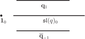
Figure 2.1: Decomposition of $\mathfrak{sl}(q+1)$ under $\mathbbm{R}^{+}\times{\rm SL}(q)$. The subscripts denote the $\mathbbm{R}^{+}$ charges which establish the vertical grading. At level $0$ one finds the algebra of $\mathbbm{R}^{+}\times{\rm SL}(q)$ while level $1$ and $-1$ contain an ${\rm SL}(q)$ vector and a dual vector, respectively.

We now want to make the ${\rm SL}(q+1)$ symmetry explicit. The scalars $\rho$, $A_{a}$ and ${\cal V}$ form an ${\rm SL}(q+1)/{\rm SO}(q+1)$ coset, the appropriate coset representative is defined as follows

$$\tilde{\cal V} =\begin{pmatrix}\rho^{-1}&0\\ \rho^{-1}A_{a}&\rho^{1/q}{\cal V}\end{pmatrix}\;.$$ (2.14)

Using the scalar current $\tilde{P}_{\mu}$ of $\tilde{\cal V}$, defined analogously to (2.10), the effective action takes the following compact form

$${\cal L}_{\text{eff,d=3}} =e\,R^{(3)}-e\,\text{tr}(\tilde{P}_{\mu}\tilde{P}^{\mu})+e\rho^{-3}{\cal L}_{M}\;.$$ (2.15)

The resulting equations of motion for $A_{a}$ are the integrability equations needed to reintroduce the vector fields $A^{a}_{\mu}$ via the duality equation (2.12), and by virtue of these duality equations all other equations of motion become equivalent to those derived from the previous Lagrangian (2.5).

The ${\rm SL}(q+1)$ acts on $\tilde{\cal V}$ from the left, analogous to (2.9), the according ${\rm SL}(q+1)$ matrices read

$$\tilde{\Lambda}(\Lambda,\lambda) =\begin{pmatrix}\lambda^{-1/q}&0\\ 0&\lambda^{1/q}\Lambda\end{pmatrix}\;, \tilde{\Lambda}(\kappa) =\begin{pmatrix}0&0\\ \kappa_{a}&0\end{pmatrix}\;, \tilde{\Lambda}(\tau) =\begin{pmatrix}0&\tau^{a}\\ 0&0\end{pmatrix}\;.$$ (2.16)

The transformations $\lambda$ and $\Lambda$ from (2.7) correspond to $\tilde{\Lambda}(\Lambda,\lambda)$, the shift symmetries $\kappa$ act via $\tilde{\Lambda}(\kappa)$, and the symmetry enhancement is described by the additional ${\rm SL}(q+1)$ elements $\tilde{\Lambda}(\tau)$. Left action with $\tilde{\Lambda}(\tau)$ on the coset representative $\tilde{\cal V}$ destroys the block-form (2.14), and an appropriate ${\rm SO}(q+1)$ action is necessary to restore this form. Therefore these new symmetry generators act highly nonlinear on the fields $\rho$, $A_{a}$ and ${\cal V}$.

The pure gravity case we were just discussing already shows many universal features that we will re-encounter in the following sections. In particular it is characteristic for maximal and half-maximal supergravities that the scalars arrange in the coset $G_{0}/H$, where $G_{0}$ is the global symmetry group and $H$ is its maximal compact subgroup. The formulation in terms of the coset representative ${\cal V}$ and the scalar currents $P_{\mu}$ and $Q_{\mu}$ is used throughout the whole article. Also the emergence of an enhanced symmetry group of the lower dimensional theory after appropriate dualization of gauge fields is a characteristic that will reappear in the following supergravity discussion. In the pure gravity case only vector gauge fields appear in the lower-dimensional theory, but for the supergravities also higher rank $p$-form gauge fields are present and can be dualized. Symmetry enhancement always takes place when the higher dimensional $p$-form fields give rise to scalar fields in the lower-dimensional theory. We will make this explicit in the following section.

2.2 Maximal supergravities from torus reductions

The unique supergravity theory in $D=11$ space-time dimensions contains as bosonic degrees of freedom the metric and a three-from gauge field $C_{\hat{\mu}\hat{\nu}\hat{\rho}}$ with field strength $G_{\hat{\mu}\hat{\nu}\hat{\rho}\hat{\lambda}}=4\partial_{[\hat{\mu}}C_{\hat{\nu}\hat{\rho}\hat{\lambda}]}$ and gauge symmetry $\delta C_{\hat{\mu}\hat{\nu}\hat{\rho}}=3\partial_{[\hat{\mu}}\Lambda_{\hat{\nu}\hat{\rho}]}$. The bosonic part of the Lagrangian reads [41]

$${\cal L}_{D=11} =\sqrt{-g}\left(R-{\textstyle\frac{1}{12}}\,G_{\hat{\mu}\hat{\nu}\hat{\rho}\hat{\lambda}}\,G^{\hat{\mu}\hat{\nu}\hat{\rho}\hat{\lambda}}+{\textstyle\frac{2}{72^{2}}}\,\epsilon^{\hat{\mu}\hat{\nu}\hat{\rho}\hat{\lambda}\hat{\sigma}\hat{\tau}\hat{\kappa}\hat{\tau}\hat{\chi}\hat{\theta}\hat{\xi}}\,G_{\hat{\mu}\hat{\nu}\hat{\rho}\hat{\lambda}}\,G_{\hat{\sigma}\hat{\tau}\hat{\kappa}\hat{\tau}}\,C_{\hat{\chi}\hat{\theta}\hat{\xi}}\right)\;.$$ (2.17)

We dimensional reduce this theory on a torus $T^{q}$ down to $d=11-q$ dimensions, i.e. we make the Ansatz (2.3) for the metric and demand $C_{\hat{\mu}\hat{\nu}\hat{\rho}}$ to be constant along the torus coordinates $y^{a}$, i.e.

$$\frac{\partial}{\partial y^{a}}C_{\hat{\mu}\hat{\nu}\hat{\rho}} =0$$ (2.18)

In $d$ dimensions the three-form then yields $q(q-1)(q-2)/6$ scalars $\chi_{[abc]}$, $q(q-1)/2$ vector gauge fields $B^{(1)}_{\mu[ab]}$, $q$ two-form gauge fields $B^{(2)}_{\mu\nu a}$ and one three-form gauge field $B^{(3)}_{\mu\nu\rho}$. The appropriate reduction Ansatz reads

$$\chi_{abc} =C_{abc}\;, B^{(1)}_{\mu ab} =\pi_{\mu}{}^{\hat{\mu}}\,C_{\hat{\mu}ab}\;,$$

$$B^{(2)}_{\mu\nu a} =\pi_{\mu}{}^{\hat{\mu}}\,\pi_{\nu}{}^{\hat{\nu}}\,C_{\hat{\mu}\hat{\nu}a}\;, B^{(3)}_{\mu\nu\rho} =\pi_{\mu}{}^{\hat{\mu}}\,\pi_{\nu}{}^{\hat{\nu}}\,\pi_{\rho}{}^{\hat{\rho}}\,C_{\hat{\mu}\hat{\nu}\hat{\rho}}\;,$$ (2.19)

where

$$\pi_{\mu}{}^{\hat{\mu}} =g_{\mu\nu}\,\frac{\partial x^{\nu}}{\partial x^{\hat{\nu}}}\,g^{\hat{\nu}\hat{\mu}}\,.$$ (2.20)

If we identify $x^{\hat{\mu}}=(x^{\mu},y^{a})$ we have $\partial x^{\nu}/\partial x^{\hat{\nu}}=\delta^{\mu}_{\hat{\mu}}$ and thus find

$$B^{(1)}_{\mu ab} =C_{\mu ab}-A^{c}_{\mu}C_{abc}\;,$$

$$B^{(2)}_{\mu\nu a} =C_{\mu\nu a}-2A^{b}_{[\mu}C_{\nu]ab}+A^{b}_{\mu}A^{c}_{\nu}C_{abc}\;,$$

$$B^{(3)}_{\mu\nu\rho} =C_{\mu\nu\rho}-3A^{a}_{[\mu}C_{\nu\rho]a}+3A^{a}_{[\mu}A^{b}_{\nu}C_{\rho]ab}-A^{a}_{\mu}A^{b}_{\nu}A^{c}_{\rho}C_{abc}\;.$$ (2.21)

The appearance of the Kaluza-Klein vector field $A^{a}_{\mu}$ ensures that the forms $B^{(p)}$ do not transform under the gauge (coordinate) transformations $L^{a}(x)$ that were introduced in (2.6). The forms $B^{(p)}$ and the scalars $\chi_{abc}$ transform under the torus ${\rm SL}(q)$ according to their index structure and are also charged under torus rescalings $\lambda$ under which also $\rho$ transform according to (2.7). The field strengths of the forms $B^{(p)}$ are defined by

$$F^{(2)}_{\mu\nu ab} =2\partial_{[\mu}B^{(1)}_{\nu]ab}\;,$$

$$F^{(3)}_{\mu\nu\rho a} =3\partial_{[\mu}B^{(2)}_{\nu\rho]a}+3A^{b}_{[\mu\nu}B^{(1)}_{\rho]ab}\;,$$

$$F^{(4)}_{\mu\nu\rho\lambda} =4\partial_{[\mu}B^{(3)}_{\nu\rho\lambda]}+6A^{a}_{[\mu\nu}B^{(2)}_{\rho\lambda]a}\;.$$ (2.22)

The appropriate gauge transformations of the forms $B^{(p)}$ that leave these field strengths invariant descend from those gauge transformations $\Lambda_{\hat{\mu}\hat{\nu}}$ of the $D=11$ three-form that do not depend on the internal coordinates. But also a linear dependence of $\Lambda_{\hat{\mu}\hat{\nu}}$ on the coordinates $y^{a}$ can be consistent with the Ansatz (2.18), as long as it does not depend on the space-time coordinates $x^{\mu}$. Of these additional symmetries we are interested in the particular case $\Lambda_{ab}=\kappa_{abc}\,y^{c}$, where $\kappa_{abc}$ has to be constant. These three-from gauge transformations yield a global shift symmetry of the scalars $\chi_{abc}$, but also act on the forms $B^{(p)}$ as follows

$$\delta\chi_{abc} =\kappa_{abc}\;, \delta B^{(1)}_{\mu ab} =-\kappa_{abc}\,A_{\mu}^{c}\;,$$

$$\delta B^{(2)}_{\mu\nu b} =A^{b}_{\mu}A^{c}_{\nu}\kappa_{abc}\;, \delta B^{(3)}_{\mu\nu\rho} =-A^{a}_{\mu}A^{b}_{\nu}A^{c}_{\rho}\kappa_{abc}\;.$$ (2.23)

This is a global symmetry of the effective $d$-dimensional theory whose Lagrangian reads

$${\cal L}_{\text{eff}} =eR+{\cal L}^{(3)}_{\text{kin}}+{\cal L}^{(2)}_{\text{kin}}+{\cal L}^{(1)}_{\text{kin}}+{\cal L}^{(0)}_{\text{kin}}+e\rho^{-d/(d-2)}{\cal L}_{FFA}\;,$$ (2.24)

where we have kinetic terms for the gauge fields and scalars

$${\cal L}^{(3)}_{\text{kin}} =-{\textstyle\frac{1}{12}}e\rho^{-1+6/(d-2)}F^{(4)}_{\mu\nu\rho\lambda}F^{(4)\mu\nu\rho\lambda}\;,$$

$${\cal L}^{(2)}_{\text{kin}} =-{\textstyle\frac{1}{3}}e\rho^{-1+4/(d-2)+2/q}M^{ab}F^{(3)}_{\mu\nu\rho a}F^{(3)\mu\nu\rho}_{b}\;,$$

$${\cal L}^{(1)}_{\text{kin}} =-{\textstyle\frac{1}{4}}e\rho^{18/(d-2)/q}\left(M_{ab}+2\rho^{(2-q)/q)}M^{ce}M^{df}\chi_{cda}\chi_{efb}\right)A^{a}_{\mu\nu}A^{b\mu\nu}$$

$$\qquad\qquad-e\rho^{-1+2/(d-2)+4/q}M^{ac}M^{bd}\chi_{abe}A_{\mu\nu}^{e}F^{(2)\mu\nu}_{cd}$$

$$\qquad\qquad\qquad\qquad-{\textstyle\frac{1}{2}}e\rho^{-1+2/(d-2)+4/q}M^{ac}M^{bd}F^{(2)}_{\mu\nu ab}F^{(2)\mu\nu}_{cd}\;,$$

$${\cal L}^{(0)}_{\text{kin}} =-{\textstyle\frac{1}{4}}e\text{tr}(M^{-1}\partial_{\mu}MM^{-1}\partial^{\mu}M)-{\textstyle\frac{9}{(d-2)q}}e(\rho^{-1}\partial_{\mu}\rho)(\rho^{-1}\partial^{\mu}\rho)$$

$$\qquad\qquad-{\textstyle\frac{1}{3}}e\rho^{-1+6/q}M^{ad}M^{be}M^{cf}(\partial_{\mu}\chi_{abc})(\partial^{\mu}\chi_{def})\;,$$ (2.25)

and ${\cal L}_{FFA}$ is a topological term that descends from the topological $GGC$-term in $D=11$. The form of this term and also the further analysis depends on the particular dimensions $d$ of the effective theory. In particular, the $p$-form gauge fields $B^{(p)}$ with field strengths $F^{(p+1)}$ can be dualized into $(d-p-2)$-form gauge fields $\tilde{B}^{(d-p-2)}$ with field strengths $\tilde{F}^{(d-p-1)}$. The corresponding duality equation schematically reads

$$\tilde{F}^{(d-p-1)} =\rho^{x}\,M\,*\,\left(F^{(p+1)}\,+\,\text{contributions from ${\cal L}_{FFA}$}\right)\;,$$ (2.26)

where the asterisk denotes Hodge dualization and $\rho^{x}\,M$ indicates that some appropriate combination of scalars is needed such that $F^{(d-p-1)}$ transforms dual to $F^{(p+1)}$ under ${\rm GL}(q)$. The duality equation is always such that the integrability equation is given by the equation of motion of the $p$-form. A Lagrange formulation of the theory can then be given that contains $\tilde{B}^{(d-p-2)}$ instead of $B^{(p)}$. The “standard” formulation of the $d$-dimensional supergravity is obtained if those $p$-forms are dualized for which $d-p-2<p$, i.e. the rank of the gauge fields is minimized. In even dimensions there are $p$-form fields with $d-p-2=p$. Thus there is some freedom which of these $p$-form fields appear in the Lagrangian. For $d=4$ this is the freedom of choosing a symplectic frame for the vector gauge fields ($p=1$).

We are particularly interested in the global onshell symmetry group of the effective theory. From the torus reduction one expects an $\mathbbm{R}^{+}\times{\rm SL}(q)$ symmetry group, where the $\mathbbm{R}^{+}$ factor corresponds to torus rescalings $\lambda$. For $d\leq 8$ the scalars $\chi_{abc}$ appear together with their shift symmetries (2.23). Since the $\chi_{abc}$ are charged under torus rescalings $\lambda$ their shift-symmetries $\kappa_{abc}$ are as well, i.e. the action of $\kappa_{aba}$ does not commute with the action of $\lambda$. In figures 2.4 to 2.4 the symmetry generators for $3\leq d\leq 6$ are depicted graphically. Again, the subscript at each generator denotes its charge under torus rescalings and the vertical grading of the generators corresponds to these charges. The generators of the torus transformations are uncharged under $\lambda$ and denoted by $\mathfrak{sl}(q)_{0}$, the generator of the torus rescalings itself is denoted ${\bf 1}_{0}$, and charge $+1$ is assigned to the shift symmetries $\kappa_{abc}$, thus they are denoted ${\bf 1}_{+1}$, ${\bf 4}_{+1}$ etc. — the number in bold letters indicates their representation under ${\rm SL}(q)$.

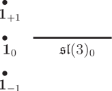
Figure 2.2: Global symmetry in $d=8$: decomposition of $\mathfrak{sl}(2)\oplus\mathfrak{sl}(3)$ under $\mathbbm{R}^{+}\times{\rm SL}(3)$.

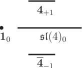
Figure 2.3: Global symmetry in $d=7$: decomposition of $\mathfrak{sl}(5)$ under $\mathbbm{R}^{+}\times{\rm SL}(4)$.

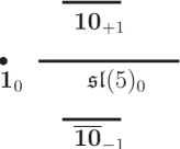
Figure 2.4: Global symmetry in $d=6$: decomposition of $\mathfrak{so}(5,5)$ under $\mathbbm{R}^{+}\times{\rm SL}(5)$.

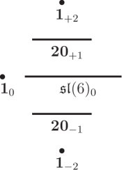
Figure 2.5: Global symmetry in $d=5$: decomposition of $\mathfrak{e}(6)$ under $\mathbbm{R}^{+}\times{\rm SL}(6)$.

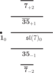
Figure 2.6: Global symmetry in $d=4$: decomposition of $\mathfrak{e}(7)$ under $\mathbbm{R}^{+}\times{\rm SL}(7)$.

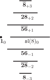
Figure 2.7: Global symmetry in $d=3$: decomposition of $\mathfrak{e}(8)$ under $\mathbbm{R}^{+}\times{\rm SL}(8)$.

Similar to the above pure gravity case in $d=3$ the symmetry group becomes miraculously enhanced. For each shift symmetry generator there also exists the dual generator with negative charge under $\lambda$ and in the dual representation of ${\rm SL}(q)$. The global symmetry group $G_{0}$ of maximal supergravity turns out to be ${\rm SL}(2)\times{\rm SL}(3)$ for $d=8$, ${\rm SL}(5)$ for $d=7$ and ${\rm SO}(5,5)$ for $d=6$. To prove this one would have to show that the kinetic term of the scalars in (2.24) describes the sigma model of the scalar cosets $G_{0}/H$ and that also the $p$-form gauge fields arrange in representations of $G_{0}$ (after dualization) such that the field equations are $G_{0}$-invariant. In even dimensions there is the subtlety of self-duality, e.g. in $d=8$ the three-form $B^{(3)}$ forms an ${\rm SL}(2)$ doublet together with its dual three-form, thus the whole global symmetry $G_{0}$ is not realized at the level of the Lagrangian but only at the level of the field equations.

For $d\leq 5$ additional scalars appear since according to (2.26) the forms $B^{(d-2)}$ can be dualized into scalars. As in the pure gravity case in $d=3$ these dual scalars also come equipped with a shift symmetry. In figures 2.7 to 2.7 the generators of these shift symmetries are denoted by ${\bf 1}_{2}$, ${\bf 7}_{2}$ and ${\bf 28}_{2}$. As before we also have the shift symmetries $\kappa_{abc}$, denoted by ${\bf 20}_{+1}$, $\overline{\bf 30}_{+1}$ and $\overline{\bf 56}_{+1}$ in the figures. For $d=3$ also the Kaluza-Klein vector fields can be dualized into scalars according to (2.12). Again, symmetry enhancement takes place, i.e. for each shift symmetry generator also the dual symmetry generator appears. This gives rise to the global symmetry group $G_{0}={\rm E}_{6(6)}$ in $d=5$, $G_{0}={\rm E}_{7(7)}$ in $d=4$, and $G_{0}={\rm E}_{8(8)}$ in $d=3$.

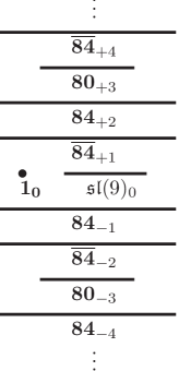
Figure 2.8: $d=2$, decomposition of $\mathfrak{e}(9)$ under ${\rm SL}(9)$.

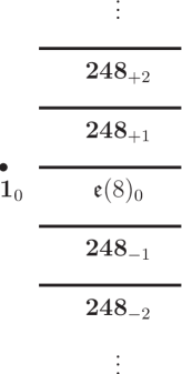
Figure 2.9: $d=2$, decomposition of $\mathfrak{e}(9)$ under $\mathbbm{R}^{+}\times{\rm E}_{8(8)}$.

For the case of $d=2$ we already mentioned that a Weyl-rescaling is not possible and thus the Lagrangian (2.24) is not the appropriate starting point for the analysis. Nevertheless, the above discussion of the field content is still applicable. From the three-form one only gets the scalars $\chi_{abc}$. The vectors and two-forms can be consistently set to zero due to their field equations. The shift symmetries of the scalars are denoted ${\bf\overline{84}}_{+1}$ in figure 2.9, and again the corresponding dual symmetries ${\bf 84}_{-1}$ arise due to symmetry enhancement. However, in $d=2$ scalars can be dualized to scalars and these new scalars can again be dualized, etc. This yields an infinite tower of new scalars and thus of new shift symmetries. Accordingly, as depicted in figure 2.9, an infinite symmetry enhancement takes place. The global symmetry group is $G_{0}={\rm E}_{9(9)}$ which is the affine extension of ${\rm E}_{8(8)}$ [42]. Thus, in contrast to higher dimensions the on-shell symmetry group is infinite-dimensional in $d=2$. The symmetry algebra is an affine Lie algebra.

To understand why the affine extension of the $d=3$ symmetry group appears here we briefly consider the reduction of the $d=3$ maximal supergravity on a torus $T^{1}$ (i.e. on a circle). This reduction yields the ${\rm E}_{8(8)}/{\rm SL}(16)$ coset of scalars in $d=2$. Onshell the dual scalars can be introduced, which transform in the adjoint representation ${\bf 248}$ of ${\rm E}_{8(8)}$; these can be dualized again to find another ${\bf 248}$ scalars, etc. This gives an infinite stack of dual scalars and shift symmetries. Symmetry enhancement yields also the dual symmetry generators, as shown in figure 2.9. From this figure it is quite intuitive that the loop group of ${\rm E}_{8(8)}$ appears as symmetry group in $d=2$. The loop group also becomes centrally extended to the affine extension ${\rm E}_{9(9)}$ of ${\rm E}_{8(8)}$. Note that in figure 2.9 the charges that are indicated as subscripts correspond to the ($d=3\rightarrow d=2$) torus rescalings $\lambda$. These torus rescalings correspond to the generator $L_{0}$ of the Virasoro algebra associated to ${\rm E}_{9(9)}$. In chapter 7 we will come back to the $d=2$ theories and also give the ${\rm E}_{9(9)}$ symmetry action explicitly. We will then also relate figures 2.9 and 2.9 by explaining the appropriate embedding of the torus ${\rm GL}(9)$ into ${\rm E}_{9(9)}$.

$d$	$G_{0}$	$H$	$p=1$	$p=2$	$p=3$	$p=4$	$p=5$
$8$	${\rm SL}(2)\times{\rm SL}(3)$	${\rm SO}(2)\times{\rm SO}(3)$	${\bf(2,3)}$	${\bf{(1,\overline{3})}}$	${\bf(2,1)}$	${\bf(1,3)}$	${\bf(2,\overline{3})}$
$7$	${\rm SL}(5)$	${\rm SO}(5)$	$\overline{\bf 10}$	${\bf 5}$	$\overline{\bf 5}$	${\bf 10}$	${\bf 24}$
$6$	${\rm SO}(5,5)$	${\rm SO}(5)\times{\rm SO}(5)$	${\bf 16_{s}}$	${\bf 10}$	${\bf 16_{c}}$	${\bf 45}$	—
$5$	${\rm E}_{6(6)}$	${\rm USp}(8)$	${\bf\overline{27}}$	${\bf 27}$	${\bf 78}$	—	—
$4$	${\rm E}_{7(7)}$	${\rm SU}(8)$	${\bf 56}$	${\bf 133}$	—	—	—
$3$	${\rm E}_{8(8)}$	${\rm SO}(16)$	${\bf 248}$	—	—	—	—
$2$	${\rm E}_{9(9)}$	$K({\rm E}_{9})$	—	—	—	—	—

Table 2.1: For the maximal supergravities in $d$ dimensions the symmetry group $G_{0}$, its maximal compact subgroup $H$ and the representations of the $p$-form gauge fields ($p\leq 5$) are listed. For $d=8$ one also has a $6$-form that transforms as ${\bf(3,1)}\oplus{\bf(1,8)}$. We also listed those $p$-forms (in $d=2$ scalars) that can be introduced onshell via dualization, i.e. not all of the above fields carry independent degrees of freedoms.

In table 2.1 we summarize the symmetry groups $G_{0}$, the scalar cosets $G_{0}/H$ and the representations of the $p$-form gauge fields for the maximal supergravities in $2\leq d\leq 8$. The global symmetry group in dimensions $2\leq d\leq 8$ turns out to be ${\rm E}_{q(q)}$, where $q=11-d$ is the dimension of the internal torus. The Dynkin diagrams of the corresponding Lie algebras are depicted in figure 2.10. Note that the standard notation for what we call $E_{3}$, $E_{4}$ and $E_{5}$ would be $A_{1}\times A_{2}$, $A_{4}$ and $D_{5}$, but it is obviously very convenient to depart from this in the present context.

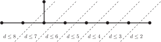
Figure 2.10: Dynkin diagram of $E_{11-d}$. For $d=8$ only the three knots on the left are present. For every decrease in dimension one additional knot occurs, i.e. the rank increases by one. Eventually, for $d=2$ one has $9$ knots and the above Dynkin diagram describes an affine Lie algebra.

All maximal supergravities that are obtained from $D=11$ supergravity are non-chiral, i.e. there is an equal number of left- and right-handed supercharges in their supersymmetry algebra. However, this distinction between left- and right-handed spinors only exists in $d=10$, $d=6$ and $d=2$. In all other dimensions there are no Weyl-spinors and the maximal supergravities are unique, but also in $d=6$ and $d=2$ only the non-chiral supergravities are of interest here, since for example in $d=6$ the chiral theories do not contain the metric in their spectrum [43, 44]. However, in ten dimensions the chiral IIB supergravity is as important as the non-chiral IIA supergravity; each describes the low-energy limit of the corresponding string theory.

The bosonic Lagrangian of the IIA theory is given by (2.24) for $d=10$, the global symmetry group is only the $\mathbbm{R}^{+}$ that corresponds to the circle rescalings. Note that in this case $B^{(1)}_{\mu ab}=0$ and $\chi_{abc}=0$, thus the bosonic field content consists of the dilaton $\rho$, one Kaluza-Klein vector $A_{\mu}^{a}$, one two-form $B^{(2)}_{\mu\nu a}$ ($a=1$) and one three-from $B^{(3)}_{\mu\nu\rho}$ — of course, the corresponding dual forms can also be introduced onshell. In contrast, the IIB supergravity possesses a global ${\rm SL}(2)$ symmetry and its bosonic field content consists of two scalars (the dilaton and the axion) that form an ${\rm SL}(2)/{\rm SO}(2)$ coset, two two-form gauge fields that form a doublet under ${\rm SL}(2)$ and one self-dual four-form gauge field. We do not need the field equations of IIB supergravity here, but we want to mention that there is no complete Lorentz invariant Lagrange formulation of the theory since the self-duality condition of the four-form gauge fields always needs to be imposed as an extra constraint.

The existence of IIB supergravity and its ${\rm SL}(2)$ symmetry help to explain the symmetry enhancement of the maximal lower dimensional supergravities, because all these theories can also be obtained from torus reduction of IIB supergravity. For $d=9$ the symmetry group of the maximal supergravity is $G_{0}=\mathbbm{R}^{+}\times{\rm SL}(2)$ and there is no symmetry enhancements, yet. Reduction from $D=11$ explains $G_{0}$ as the symmetry group of the internal torus $T^{2}$, and reduction from IIB supergravity explains it as the product of the ten-dimensional ${\rm SL}(2)$ symmetry and the $\mathbbm{R}^{+}$ (rescaling) symmetry of the internal circle. But for $d=8$ one expects an $G_{a}=\mathbbm{R}^{+}\times{\rm SL}(3)$ symmetry from $T^{3}$ reduction of $D=11$, and an $G_{b}=\mathbbm{R}^{+}\times{\rm SL}(2)\times{\rm SL}(2)$ symmetry from $T^{2}$ reduction of IIB. Neither $G_{a}$ is a subgroup of $G_{b}$ nor vice versa, but they are both contained in the complete global symmetry group $G_{0}={\rm SL}(2)\times{\rm SL}(3)$ and a careful analysis shows that $G_{a}$ and $G_{b}$ even generate this group. The analysis for dimensions $d\leq 7$ is analogous.

So the miracle of symmetry enhancement is explained by the miracle of having different higher-dimensional ancestors for the same effective theory. From a string theory perspective this is the miracle of $T$-duality ($T$ refers to torus) which states that IIA and IIB string theory are identical when compactified on a torus $T^{q}$, i.e. when the target manifold is of the form ${\cal M}_{d}\times T^{q}$. Being identical means that they are just two different formulations of the same theory, and this statements holds beyond the effective lower-dimensional supergravity, i.e. also for the whole tower of massive string states. However, when the whole string theory is considered it turns out that the symmetry group is no longer the real Lie group ${\rm E}_{11-d(11-d)}$, but only its discrete subgroup ${\rm E}_{11-d(11-d)}(\mathbbm{Z})$, which is referred to as $U$-duality groups in a string theory context. One should keep in mind the duality origin of these global symmetry groups, although here we will not pursue the string theory roots further.

2.3 Half-maximal supergravities

We now want to depict the ungauged half-maximal supergravities, i.e. those with $Q=16$ real supercharges in their supersymmetry algebra. Again we restrict the discussion to the non-chiral supergravities, thus avoiding subtleties in $d=6$ and $d=2$ dimensions. Concerning the field content of half-maximal supergravity one does not have much freedom since the bosonic and fermionic states have to arrange in multiplets of the supersymmetry algebra. For the maximal $Q=32$ theories there is only one possible multiplet, the $Q=32$ gravity multiplet. For the half-maximal theories there are two types of multiplets: the $Q=16$ gravity and the $Q=16$ vector multiplet. One gravity multiplet is always needed since it contains the metric, but in addition there is the freedom of adding $m\in\mathbbm{N}$ vector multiplets.

The supersymmetry structure is still very rigid for $Q=16$. For the ungauged theory there is only one way to consistently couple the vector multiplets to the gravity multiplet, i.e. the ungauged theory is completely determined when one specifies the dimension $d$ and the number $m$ of vector multiplets. In dimensions $d\neq 6$ gaugings are the only known deformations of these half-maximal supergravities that are compatible with supersymmetry. For $d=6$ one has the additional freedom to couple the vector fields to the two-form gauge field of the gravitational multiplet via Stückelberg type couplings [16]. We will introduce these type of couplings also for the gauged theories in all dimensions $d\geq 4$, but the difference in $d=6$ is that it can be switched on in addition to the gauging or without a gauging. This is analogous to IIA maximal supergravity in $d=10$, where also a massive deformation exists which is not a gauging [15].

The $Q=16$ supergravities in $d$ dimensions can be obtained from torus reductions of $Q=16$ (i.e. $N=1$) supergravity in ten dimensions. The $Q=16$, $d=10$ gravity multiplet contains as bosonic fields the metric, a scalar $\phi$ called the dilaton and an antisymmetric two-form gauge field $B_{\mu\nu}$. We label the vector multiplets by $i=1,\ldots,m$. Each vector multiplet contains only one vector gauge field $A^{i}_{\mu}$ as bosonic degrees of freedom. The bosonic Lagrangian in the Einstein frame reads [45, 46, 47]

$${\cal L}_{D=10} =\sqrt{-g}\left(R-{\textstyle\frac{9}{8}}(\phi^{-1}\partial_{\mu}\phi)(\phi^{-1}\partial^{\mu}\phi)-{\textstyle\frac{3}{2}}\phi^{-4}{\cal G}_{\mu\nu\rho}{\cal G}^{\mu\nu\rho}-{\textstyle\frac{1}{2}}\phi^{-2}{\cal F}^{i}_{\mu\nu}{\cal F}^{i\,\mu\nu}\right)\;,$$ (2.27)

where ${\cal F}^{i}_{\mu\nu}=2\partial_{[\mu}A^{i}_{\nu]}$ and ${\cal G}_{\mu\nu\rho}=3\partial_{[\mu}B_{\nu\rho]}-A^{i}_{[\mu}F^{i}_{\nu\rho]}$ are the Abelian field strengths of the vector-and two-form gauge fields. This Lagrangian is invariant under ${\rm SO}(m)$ rotations on the vector fields $A_{\mu}^{i}$ and under rescaling $\phi\mapsto\varphi\,\phi$, $B_{\mu\nu}\mapsto\varphi^{2}\,B_{\mu\nu}$ and $A^{i}_{\mu}\mapsto\varphi\,A^{i}_{\mu}$, where $\varphi\in\mathbbm{R}^{+}$. Thus the global symmetry group is $G_{0}=\mathbbm{R}^{+}\times{\rm SO}(m)$. On can deform the theory by gauging a subgroup of $G_{0}$, using the $A_{\mu}^{i}$ as gauge fields. A particularly important example is the case $m=496$ and a subgroup ${\rm E}_{8}\times{\rm E}_{8}$ or ${\rm SO}(32)$ gauged. In these cases the appropriate deformation of the Lagrangian (2.27) describes the low energy limit of type I and heterotic string theory. But we continue to consider the ungauged theory further.

When compactifying to $d=10-q$ dimensions the two form $B_{\mu\nu}$ yields one two-form, $q$ vector fields and $q(q-1)/2$ scalars in the effective theory, while the vector fields $A_{\mu}^{i}$ yield $m$ vector fields and $m\cdot q$ scalars. In total one thus obtains $n=m+q$ vector fields from the gauge fields of $D=10$. For $d\geq 4$ this is also the number of vector multiplets one encounters in $d$ dimensions. In other words, the $Q=16$ gravity multiplet in $d+1$ dimensions always decomposes into one gravity and one vector multiplet in $d$ dimensions. For $d=3$ an additional “vector-multiplet” appears since the dilaton from the metric can be dualized into a vector field and we then have $n=m+q+1$.

The analysis of the symmetry group $G_{0}$ of the effective theory is analogous to the discussion in the last section, i.e. whenever a new scalar field appears it comes equipped with a shift symmetry and there is a symmetry enhancement by the generators dual to these shift symmetries. This yields the global symmetry group $G_{0}=\mathbbm{R}^{+}\times{\rm SO}(q,n)$ for $5\leq d\leq 9$. In $d=4$ also the two-form can be dualized to a scalar and the symmetry group becomes enlarged to $G_{0}={\rm SL}(2)\times{\rm SL}(q,n)$. Similarly, for $d=3$ the vector fields yield scalars via dualization such that the global symmetry group becomes $G_{0}={\rm SO}(8,n)$, and for $d=2$ the affine extension of the three-dimensional symmetry group is obtained. As in the maximal case it turns out that the scalars always form a scalar coset $G_{0}/H$. The respective maximal subgroups $H$ and the remaining bosonic fields are summarized in table 2.2. Note that one obtains only $n\geq q$ (respectively $n\geq q+1$ for $d=3$) from torus reduction of $D=10$, but there are $d$-dimensional theories for all numbers of vector multiplets $n\in\mathbbm{N}$.

$d$	$G_{0}$	$H$	$p=1$	$p=2$
$8$	$\mathbbm{R}^{+}\times{\rm SO}(2,n)$	${\rm SO}(2)\times{\rm SO}(n)$	${\bf(2+n)_{+1/2}}$	${\bf{1}_{+1}}$
$7$	$\mathbbm{R}^{+}\times{\rm SO}(3,n)$	${\rm SO}(3)\times{\rm SO}(n)$	${\bf(3+n)_{+1/2}}$	${\bf 1}_{+1}$
$6$	$\mathbbm{R}^{+}\times{\rm SO}(4,n)$	${\rm SO}(4)\times{\rm SO}(n)$	${\bf(4+n)_{+1/2}}$	${\bf 1}_{+1}\oplus{\bf 1}_{-1}$
$5$	$\mathbbm{R}^{+}\times{\rm SO}(5,n)$	${\rm SO}(5)\times{\rm SO}(n)$	${\bf(5+n)_{+1/2}\oplus 1_{-1}}$	${\bf(5+n)_{-1/2}\oplus 1_{+1}}$
$4$	${\rm SL}(2)\times{\rm SO}(6,n)$	${\rm SO}(6)\times{\rm SO}(n)$	${\bf(2,6+n)}$	$\text{\bf adj}_{G_{0}}$
$3$	${\rm SO}(8,n)$	${\rm SO}(8)\times{\rm SO}(n)$	$\text{\bf adj}_{G_{0}}$	—

Table 2.2: For the $d$ dimensional half-maximal supergravities coupled to $n$ vector multiplets the symmetry group $G_{0}$, its maximal compact subgroup $H$ and the representations of the vector and two-form gauge fields are listed. The subscripts at the representations denote the $\mathbbm{R}^{+}$ charges. The $(d-2-p)$-forms always transform dual to the $p$-forms and the $p=d-2$ forms always transform in the adjoint representation of $G_{0}$. Note the respective dual forms can only be introduced onshell and only those fields that appear in the ungauged Lagrangian carry degrees of freedom.

Chapter 3 The general structure of gauged supergravity theories

In this chapter we start with some supersymmetric theory with global symmetry group $G_{0}$ and ask for the possible gaugings of this theory that are compatible with supersymmetry, i.e. we demand the deformations of the theory not to break supersymmetry. Although the answer to this question needs a case by case study, there exists a general technique to parameterize the deformations via an embedding tensor $\Theta$, which is a tensor under the global symmetry group $G_{0}$ and has to satisfy certain group theoretical constraints. Every single gauging breaks the global symmetry $G_{0}$ down to a local gauge group $G\subset G_{0}$, but the set of all possible gaugings can be described in a $G_{0}$ covariant way by using $\Theta$. This embedding tensor and the constraints it has to satisfy are introduced in the following section for an arbitrary theory, and as far as possible we try to keep this generality in the remainder of this chapter. However, eventually we always specialize to the maximal and half-maximal supergravities that were introduced in the last chapter.

3.1 The embedding tensor

We start from an ungauged supersymmetric theory with global symmetry group $G_{0}$. The symmetry generators of the corresponding algebra $\mathfrak{g}_{0}$ are denotes $t_{\alpha}$, $\alpha=1,\ldots,\dim(\mathfrak{g}_{0})$. They obey

$$[t_{\alpha},t_{\beta}] =f_{\alpha\beta}{}^{\gamma}\,t_{\gamma}\;,$$ (3.1)

where $f_{\alpha\beta}{}^{\gamma}$ are the structure constants of $G_{0}$. Gauging the theory means to turn part of this global symmetry into a local one. In order to preserve gauge invariance one needs to introduce minimal couplings of vector gauge fields, i.e. one replaces derivatives $\partial_{\mu}$ by covariant derivatives $D_{\mu}$. The theory to start with contains vector fields $A_{\mu}^{M}$ that transform in some representation $V$ (indicated by the index $M$) of the global symmetry group $G_{0}$. These vector fields are ${\rm U}(1)$ gauge fields, i.e. they do not only transform under $\mathfrak{g}_{0}$-transformations $L^{\alpha}$, but also under local gauge transformations $\Lambda^{M}(x)$:

$$\delta_{L}A_{\mu}^{M} =-L^{\alpha}\,t_{\alpha N}{}^{M}\,A_{\mu}^{N}\;, \delta_{\Lambda}A_{\mu}^{M} =\partial_{\mu}\Lambda^{M}\;.$$ (3.2)

In the covariant derivative of the gauged theory these vector fields $A_{\mu}^{M}$ need to be coupled to the $G_{0}$ symmetry generators $t_{\alpha}$, i.e. [29]

$$D_{\mu} =\partial_{\mu}-\,g\,A_{\mu}^{M}\,\Theta_{M}{}^{\alpha}\,t_{\alpha}\;,$$ (3.3)

where $\Theta_{M}{}^{\alpha}$ is the so-called embedding tensor and $g\in\mathbbm{R}$ is the gauge coupling constant, which could also be absorbed into $\Theta_{M}{}^{\alpha}$. The embedding tensor $\Theta_{M}{}^{\alpha}$ has to be real and appears in (3.3) as a map $\Theta\,:\,V\,\rightarrow\,\mathfrak{g}_{0}$. The image of this map defines the gauge group $G$ and the possible gauge transformations are parameterized by $\Lambda^{M}(x)$. For example, a field $B_{M}$ in the dual representation $\overline{V}$ of the vector gauge fields transforms under $G$ as

$$\delta B_{M} =g\,\Lambda^{N}\,\Theta_{N}{}^{\alpha}\,t_{\alpha M}{}^{P}\,B_{P}=g\,\Lambda^{N}\,X_{NM}{}^{P}\,B_{P}\;.$$ (3.4)

Here we introduced the gauge group generators $X_{M}=\Theta_{M}{}^{\alpha}t_{\alpha}$, which in the vector field representation $X_{MN}{}^{P}=\Theta_{M}{}^{\alpha}\,t_{\alpha N}{}^{P}$ take the role of generalized structure constants for the gauge group $G$. Note that $X_{MN}{}^{P}$ contains the whole information on $\Theta$ if the vector field representation is faithful. The embedding tensor is not invariant under the global symmetry group $G_{0}$, but to ensure the closure of the gauge group and the gauge covariance of the following construction we demand $\Theta$ to be invariant under gauge transformations $\delta=\Lambda^{M}\delta_{M}$, i.e.

$$\delta_{M}\Theta_{N}{}^{\alpha} =g\Theta_{M}{}^{\beta}\left(t_{\beta N}{}^{P}\,\Theta_{P}{}^{\alpha}-f_{\beta\gamma}{}^{\alpha}\,\Theta_{N}{}^{\gamma}\right)=0\;.$$ (3.5)

Equivalently one can demand the generators $X_{MN}{}^{P}$ to be gauge invariant, and the equation $\delta_{M}X_{NP}{}^{Q}=0$ can be written as

$$[X_{M},X_{N}] =-X_{MN}{}^{P}\,X_{P}\;.$$ (3.6)

This equation guarantees the closure of the gauge group and is the generalized Jacobi identity when evaluated in the vector field representation. Note that the generators $X_{MN}{}^{P}$ are generically not antisymmetric in the first two indices, and equation (3.6) only demands this antisymmetry under projection with $X_{P}$, that is with $\Theta_{M}{}^{\alpha}$. The two equivalent relations (3.5) and (3.6) represent a quadratic constraint on $\Theta$. The embedding tensor has to satisfy this constraint in order to describe a valid gauging.

In addition to this quadratic constraint a linear constraint on $\Theta$ is needed as well. Eventually, it is supersymmetry which demands this linear constraint, but we will see in section 3.2 that already the gauge invariance of the vector and tensor gauge field system yield at least parts of this linear constraint. The embedding tensor transforms in the representation $\overline{V}\otimes\mathfrak{g}_{0}=\theta_{1}\oplus\theta_{2}\oplus\ldots\oplus\theta_{n}$, where $\theta_{i}$, $i=1,\ldots,n$, are the irreducible components of the tensor product. The linear constraint needs to be $G_{0}$ invariant. Thus, each irreducible component $\theta_{i}$ is either completely forbidden by the linear constraint or not restricted at all, i.e. there is a subset $S\subset\{1,\ldots,n\}$ such that the linear constraint reads

$$\theta_{i} =0\qquad\text{for all }i\in S\;.$$ (3.7)

This equation can be written as a projector equation $\mathbbm{P}_{1}\Theta=0$, where $\mathbbm{P}_{1}$ projects onto those representation in $\Theta$ that are forbidden. Similarly, the quadratic constraint can be written as $\mathbbm{P}_{2}(\Theta\otimes\Theta)=0$, where $\mathbbm{P}_{2}$ projects on the appropriate representation in the symmetric tensor product of $\overline{V}\otimes\mathfrak{g}_{0}$. One could also imagine higher order constraints like $\mathbbm{P}_{3}(\Theta\otimes\Theta\otimes\Theta)=0$, but it turns out that the linear and quadratic constraint are sufficient for the construction of the gauged theories.

For the maximal and half-maximal supergravities the global symmetry group $G_{0}$ and the representation $V$ of the vector fields were given in tables 2.1 and 2.2. For the known cases we collected the linear constraint in tables 3.1 and 3.2. For the maximal theories a similar table was given in [48, 49]. For the odd dimensions, i.e. $d=3$, $d=5$ and $d=7$, the maximal gauged theories were worked out explicitly [30, 33, 34], but via torus reduction one can infer the linear constraint for the even dimensions $d\geq 4$ as well — in appendix A this is explained in detail. By applying the methods of [50] one can also describe explicitly the general gaugings of maximal $d=4$ supergravity [32]. The maximal theories for $d=8$ and $d=6$ were not yet worked out completely. The maximal $d=2$ theory will be considered in chapter 7. For the half-maximal theories we refer to [31, 25, 35] and to chapters 4 and 5.

$d$	$G_{0}$	$\mathfrak{g}_{0}\otimes\overline{V}$  $=$	allowed  $\oplus$	forbidden
$8$	${\rm SL}(2)\times{\rm SL}(3)$	$\mathfrak{g}_{0}\otimes{\bf(2,\overline{3})}$  $=$	${\bf(2,\overline{3})}\oplus{\bf(2,6)}$  $\oplus$	${\bf(2,\overline{3})}\oplus{\bf(2,\overline{15})}\oplus{\bf(4,\overline{3})}$
$7$	${\rm SL}(5)$	${\bf 24}\otimes{\bf 10}$  $=$	${\bf 15}\oplus\overline{\bf 40}$  $\oplus$	${\bf 10}\oplus{\bf 175}$
$6$	${\rm SO}(5,5)$	${\bf 45}\otimes{\bf 16}_{c}$  $=$	${\bf 144}_{s}$  $\oplus$	${\bf 16}_{c}\oplus{\bf 560}_{c}$
$5$	${\rm E}_{6(6)}$	${\bf 78}\otimes{\bf 27}$  $=$	$\overline{\bf 351}$  $\oplus$	${\bf 27}\oplus{\bf 1728}$
$4$	${\rm E}_{7(7)}$	${\bf 133}\otimes{\bf 56}$  $=$	${\bf 912}$  $\oplus$	${\bf 56}\oplus{\bf 6480}$
$3$	${\rm E}_{8(8)}$	${\bf 248}\otimes{\bf 248}$  $=$	${\bf 1}\oplus{\bf 3875}$  $\oplus$	${\bf 248}\oplus{\bf 27000}\oplus{\bf 30380}$
$2$	${\rm E}_{9(9)}$	$\mathfrak{g}_{0}\otimes\text{\bf basic}$  $=$	basic  $\oplus$	rest

Table 3.1: Decomposition of $\Theta$ for the $d$ dimensional maximal supergravities. The linear constraint only allows some of the irreducible components of $\Theta$. For $d=8$ we have $\mathfrak{g}_{0}={\bf(3,1)}\oplus{\bf(1,8)}$. For $d=2$ the algebra is the affine extension of $\mathfrak{e}_{8(8)}$ and the vector fields transform in the unique level one representation, called the basic representation — see chapter 7.

$d$	$\mathfrak{g}_{0}$  $\otimes$	$\overline{V}$  $=$	allowed   $\oplus$	forbidden
$5$	$\Big{(}{\bf 1}_{0}\;\oplus\;$ $\mbox{\tiny \vbox{\vskip 3.0pt plus 1.0pt minus 1.0pt\offinterlineskip\halign{&\vsquare{#}\cr\vbox{\hbox{\vrule width=0.4pt\vbox to7.0pt{\hrule height=0.4pt\vss\hbox to7.0pt{\hss$$\hss} \vss\hrule height=0.4pt} \vrule width=0.4pt} \kern-0.4pt}\kern-0.4pt\cr\vbox{\hbox{\vrule width=0.4pt\vbox to7.0pt{\hrule height=0.4pt\vss\hbox to7.0pt{\hss$$\hss} \vss\hrule height=0.4pt} \vrule width=0.4pt} \kern-0.4pt}\kern-0.4pt\cr}}}_{\,0}$ $\Big{)}$  $\otimes$	$\Big{(}{\bf 1}_{1}\;\oplus\;$ $\mbox{\tiny \vbox{\vskip 3.0pt plus 1.0pt minus 1.0pt\offinterlineskip\halign{&\vsquare{#}\cr\vbox{\hbox{\vrule width=0.4pt\vbox to7.0pt{\hrule height=0.4pt\vss\hbox to7.0pt{\hss$$\hss} \vss\hrule height=0.4pt} \vrule width=0.4pt} \kern-0.4pt}\kern-0.4pt\cr}}}_{\,-1/2}$ $\Big{)}$  $=$	$\mbox{\tiny \vbox{\vskip 3.0pt plus 1.0pt minus 1.0pt\offinterlineskip\halign{&\vsquare{#}\cr\vbox{\hbox{\vrule width=0.4pt\vbox to7.0pt{\hrule height=0.4pt\vss\hbox to7.0pt{\hss$$\hss} \vss\hrule height=0.4pt} \vrule width=0.4pt} \kern-0.4pt}\kern-0.4pt\cr}}}_{\,-1/2}$ $\oplus\,$ $\mbox{\tiny \vbox{\vskip 3.0pt plus 1.0pt minus 1.0pt\offinterlineskip\halign{&\vsquare{#}\cr\vbox{\hbox{\vrule width=0.4pt\vbox to7.0pt{\hrule height=0.4pt\vss\hbox to7.0pt{\hss$$\hss} \vss\hrule height=0.4pt} \vrule width=0.4pt} \kern-0.4pt}\kern-0.4pt\cr\vbox{\hbox{\vrule width=0.4pt\vbox to7.0pt{\hrule height=0.4pt\vss\hbox to7.0pt{\hss$$\hss} \vss\hrule height=0.4pt} \vrule width=0.4pt} \kern-0.4pt}\kern-0.4pt\cr}}}_{\,1}$ $\oplus\,$ $\mbox{\tiny \vbox{\vskip 3.0pt plus 1.0pt minus 1.0pt\offinterlineskip\halign{&\vsquare{#}\cr\vbox{\hbox{\vrule width=0.4pt\vbox to7.0pt{\hrule height=0.4pt\vss\hbox to7.0pt{\hss$$\hss} \vss\hrule height=0.4pt} \vrule width=0.4pt} \kern-0.4pt}\kern-0.4pt\cr\vbox{\hbox{\vrule width=0.4pt\vbox to7.0pt{\hrule height=0.4pt\vss\hbox to7.0pt{\hss$$\hss} \vss\hrule height=0.4pt} \vrule width=0.4pt} \kern-0.4pt}\kern-0.4pt\cr\vbox{\hbox{\vrule width=0.4pt\vbox to7.0pt{\hrule height=0.4pt\vss\hbox to7.0pt{\hss$$\hss} \vss\hrule height=0.4pt} \vrule width=0.4pt} \kern-0.4pt}\kern-0.4pt\cr}}}_{\,-1/2}$   $\oplus$	${\bf 1}_{1}\oplus\,$ $\mbox{\tiny \vbox{\vskip 3.0pt plus 1.0pt minus 1.0pt\offinterlineskip\halign{&\vsquare{#}\cr\vbox{\hbox{\vrule width=0.4pt\vbox to7.0pt{\hrule height=0.4pt\vss\hbox to7.0pt{\hss$$\hss} \vss\hrule height=0.4pt} \vrule width=0.4pt} \kern-0.4pt}\kern-0.4pt\cr}}}_{\,-1/2}$ $\oplus\,$ $\mbox{\tiny \vbox{\vskip 3.0pt plus 1.0pt minus 1.0pt\offinterlineskip\halign{&\vsquare{#}\cr\vbox{\hbox{\vrule width=0.4pt\vbox to7.0pt{\hrule height=0.4pt\vss\hbox to7.0pt{\hss$$\hss} \vss\hrule height=0.4pt} \vrule width=0.4pt} \kern-0.4pt}\kern-0.4pt&\vbox{\hbox{\vrule width=0.4pt\vbox to7.0pt{\hrule height=0.4pt\vss\hbox to7.0pt{\hss$$\hss} \vss\hrule height=0.4pt} \vrule width=0.4pt} \kern-0.4pt}\kern-0.4pt\cr\vbox{\hbox{\vrule width=0.4pt\vbox to7.0pt{\hrule height=0.4pt\vss\hbox to7.0pt{\hss$$\hss} \vss\hrule height=0.4pt} \vrule width=0.4pt} \kern-0.4pt}\kern-0.4pt\cr}}}_{\vspace{0.2cm}-1/2}$
$4$	$\big{[}({\bf 3},\cdot)\oplus({\bf 1},$                 $)\big{]}$  $\otimes$	$({\bf 2},$         $)$  $=$	$({\bf 2},$         $)$ $\oplus$ $({\bf 2},$                         $)$   $\oplus$	$({\bf 2},$         $)$ $\oplus$ $\ldots$
$3$	$\otimes$	$=$	1 $\;\oplus\;$                 $\;\oplus\;$                                   $\oplus$	$\;\oplus\;$                                 $\;\oplus\;$

Table 3.2: Decomposition of $\Theta$ for the $d$ dimensional half-maximal supergravities. The linear constraint only allows some of the irreducible components of $\Theta$. For $d=5$ the global symmetry group $G_{0}$ is $\mathbbm{R}^{+}\times{\rm SO}(5,n)$, and the $\mathbbm{R}^{+}$ charges are given as subscripts. For $d=4$ and $d=3$ we have $G_{0}={\rm SL}(2)\times{\rm SO}(6,n)$ and $G_{0}={\rm SO}(8,n)$, respectively, where $n$ is the number of vector multiplets. The Yang-tableaus always refer to the respective ${\rm SO}$-group.

It should be mentioned that table 3.1 and 3.2 reflect our present knowledge of the methods that can be used to work out the general gauged theories. It is not impossible that a weaker linear constraints might suffice, if new methods are applied in the future. In this respect the linear constraint is less robust than the quadratic one, which can immediately be traced back to gauge invariance and closure of the gauge group.

We summarize this section. When describing the general gauging of a supersymmetric theory, the embedding tensor $\Theta$ can be used to parameterize the gauging. Any $\Theta$ that satisfies the appropriate linear constraint (3.7) and the quadratic constraint (3.5) describes a valid gauging and the construction of the gauged theory only requires these constraints for consistency. When $\Theta$ is treated as a spurionic object, i.e. it transforms under the global symmetry group $G_{0}$, one does formally preserve the $G_{0}$ symmetry in the gauged theory. This reflects the fact that the set of all possible gaugings is $G_{0}$ invariant. But as soon as a particular gauging is considered, the embedding tensor that describes this gauging breaks the $G_{0}$ invariance down to the gauge group $G\subset G_{0}$.

3.2 Non-Abelian vector and tensor gauge fields

In this section we mainly present the results of [52] on the general form of vector/tensor gauge transformations in arbitrary space-time dimensions, but translated into a more convenient basis, see also the appendix of [34].

3.2.1 Gauge transformations and covariant field strengths

First, we want to introduce the gauge transformations and covariant field strengths for the $p$-form gauge fields that appear in gauged supergravity theories. Explicitly we will give all formulas for rank $p\leq 3$, but in principle the construction can be continued to arbitrary rank. It will turn out that always the $(p+1)$-forms are needed to define a gauge invariant field strengths for the $p$-forms. In the next subsection we will explain how to truncate this tower of gauge fields to a finite subset without loosing gauge invariance.

In the ungauged theory we have (at least onshell) vector gauge fields $A_{\mu}^{M}$, two-form gauge fields $B_{\mu\nu\,I}$, three form-gauge fields $S^{A}_{\mu\nu\rho}$, etc., and all these fields come in possibly different representation of the global symmetry group $G_{0}$, indicated by the indices $M$, $I$ and $A$. The Abelian field strengths of these tensor gauge fields take the form

$${\cal F}^{0,M}_{\mu\nu} =2\,\partial_{[\mu}\,A^{M}_{\nu]}$$

$${\cal F}^{0}_{\mu\nu\rho\,I} =3\,\partial_{[\mu}\,B_{\nu\rho]I}+6\,d_{IMN}\,A_{[\mu}^{M}\,\partial_{\nu}\,A_{\rho]}^{N}\;,$$

$${\cal F}^{0,A}_{\mu\nu\rho\lambda} =4\,\partial_{[\mu}\,S^{A}_{\nu\rho\lambda]}-c^{AI}_{M}\,\left(12\,B_{[\mu\nu\,I}\,\partial_{\rho}A^{M}_{\lambda]}+8\,d_{INP}\,A^{M}_{[\mu}\,A^{N}_{\nu}\,\partial_{\rho}\,A^{P}_{\lambda]}\right)\;,$$ (3.8)

where $d_{IMN}$ and $c^{AI}_{M}$ are some appropriate $G_{0}$-invariant tensors. To ensure invariance under the Abelian gauge transformations these tensors have to satisfy

$$d_{I[MN]} =0\;, d_{I(MN}\,c^{AI}_{P)} =0\;.$$ (3.9)

The existence of $d_{IMN}=d_{I(MN)}$ means that the two-fold symmetric tensor product of the representation of the vector-fields $A_{\mu}^{M}$ contains the representation of the two-form fields $B_{\mu\nu\,I}$. Similarly, the existence of $c^{AI}_{M}$ means that the representation of $S_{\mu\nu\rho}^{A}$ is contained in the tensor product of the representations of $A_{\mu}^{M}$ and $B_{\mu\nu\,I}$. Using table 2.1 one can easily check that these conditions are satisfied for the maximal supergravities. The second equation in (3.9) also holds since the three-fold symmetric tensor product of the vector field-representation never contains the representation of ${\rm S_{\mu\nu\rho}^{A}}$.

We saw in chapter 2 that in dimensional reduction of $D=11$ supergravity additional terms $A\partial A$, etc., appear naturally in the field strength of the higher rank tensor fields. From a lower dimensional perspective these terms are very important for anomaly cancellation, and therefore always present. Using the relations (3.9) one can show that under arbitrary variations $\delta A_{\mu}^{M}$, $\delta B_{\mu\nu\,I}$ and $\delta S^{A}_{\mu\nu\rho}$ the field strengths vary as

$$\delta\,{\cal F}_{\mu\nu}^{0,M} =2\,\partial_{[\mu}\,(\Delta A_{\nu]}^{M})\;,$$

$$\delta\,{\cal F}^{0}_{\mu\nu\rho\,I} =3\,\partial_{[\mu}(\Delta B_{\nu\rho]\,I})+6\,d_{IMN}\,{\cal F}_{[\mu\nu}^{0,M}\,\Delta A_{\rho]}^{N}\;,$$

$$\delta\,{\cal F}^{0,A}_{\mu\nu\rho\lambda} =4\,\partial_{[\mu}(\Delta S^{A}_{\mu\nu\rho]})-6\,c^{AI}_{M}\,{\cal F}^{0,M}_{[\mu\nu}\,\Delta B_{\rho\lambda]\,I}+4\,c^{AI}_{M}\,{\cal F}^{0}_{[\mu\nu\rho\,I}\,\Delta A^{M}_{\lambda]}\;,$$ (3.10)

where we used the “covariant variations”

$$\Delta A_{\mu}^{M} =\delta A_{\mu}^{M}\;,$$

$$\Delta B_{\mu\nu\,I} =\delta B_{\mu\nu\,I}-2d_{IMN}\,A_{[\mu}^{M}\,\delta A_{\nu]}^{N}\;,$$

$$\Delta S_{\mu\nu\rho}^{A} =\delta S_{\mu\nu\rho}^{A}-3\,c^{AI}_{M}\,B_{[\mu\nu\,I}\,\delta A^{M}_{\rho]}-2\,c^{AI}_{M}\,d_{INP}\,A^{M}_{[\mu}\,A^{N}_{\nu}\,\delta A^{P}_{\rho]}\;.$$ (3.11)

These covariant variations are very useful since they allow to express gauge transformations and variations of gauge invariant objects in a manifestly covariant form, i.e. without explicit appearance of gauge fields.

We now ask for the appropriate generalization of (3.8) in the gauged theory. The gauge group generators $X_{MN}{}^{P}$ were already introduced in the last section, and according to equation (3.6) they take the role of generalized structure constants. Therefore, it would be natural to define the non-Abelian field strength of the vector fields $A_{\mu}^{M}$ as

$${\cal F}^{M}_{\mu\nu} =2\,\partial_{[\mu}\,A^{M}_{\nu]}+gX_{NP}{}^{M}\,A_{[\mu}^{N}\,A_{\nu]}^{P}\;,$$ (3.12)

but under gauge transformations $\delta A_{\mu}^{M}=D_{\mu}\Lambda^{M}$ one finds this field strength to transform as

$$\delta{\cal F}^{M}_{\mu\nu} =2\,D_{[\mu}\delta A^{M}_{\nu]}\,=\,2\,D_{[\mu}D_{\nu]}\Lambda^{M}\,=\,g\,{\cal F}^{N}_{\mu\nu}\,X_{NP}{}^{M}\,\Lambda^{P}$$

$$=-g\,\Lambda^{N}\,X_{NP}{}^{M}\,{\cal F}^{P}_{\mu\nu}+2\,g\,\Lambda^{N}\,X_{(NP)}{}^{M}\,{\cal F}^{P}_{\mu\nu}$$ (3.13)

where we used the Ricci identity $[D_{\mu},D_{\nu}]=-g{\cal F}_{\mu\nu}^{M}X_{M}$, which is valid due to the quadratic constraint, see also [33]. Here and in the following we use the covariant derivative as defined in (3.3). In the second line of equation (3.13) the first term alone would describe the correct covariant transformation of the field strength, but there is an unwanted second term since the $X_{NP}{}^{M}$ are typically not antisymmetric in the first two indices. Thus the field strengths ${\cal F}_{\mu\nu}^{M}$ does not transform covariantly under gauge transformations.

This problem arises because the dimension of the gauge group $G$ can be smaller than the number of Abelian vector fields $A_{\mu}^{M}$, and thus not all vector fields are really needed as gauge fields. For any particular gauge group one could split the vector fields into the gauge fields and the remainder and treat them differently in the gauged theory. Those vector fields that are neither used as gauge fields for $G$ nor are sterile under $G$ have to be absorbed into massive two-forms. But an explicit split of the vector fields is not appropriate for our purposes since we search for a general formulation valid for all allowed embedding tensors. To solve this problem one introduces a covariant field strength of the vector fields that contains Stückelberg type couplings to the two-form gauge fields, i.e.

$${\cal H}^{M}_{\mu\nu} =2\,\partial_{[\mu}\,A^{M}_{\nu]}+gX_{NP}{}^{M}\,A_{[\mu}^{N}\,A_{\nu]}^{P}+gZ^{MI}B_{\mu\nu\,I}\;.$$ (3.14)

The tensor $Z^{MI}$ should be such that the unwanted terms in (3.13) can be absorbed into an appropriate gauge transformation of the two-form gauge fields. Explicitly, $\delta B_{\mu\nu\,I}$ should contain a term $(-2\,d_{INP}\,\Lambda^{N}\,{\cal F}^{P}_{\mu\nu})$ and we need

$$X_{(MN)}{}^{P} =d_{IMN}Z^{PI}\;.$$ (3.15)

This equation implicitly defines $Z^{MI}$ as a linear function of the embedding tensor, but it is also a linear constraint on $\Theta$ itself, since $X_{(MN)}{}^{P}$ not necessarily has the form (3.15). For example for the maximal supergravity in $d=7$ this already yields the complete linear constraint. Note that the quadratic constraint (3.6) implies

$$X_{(MN)}{}^{P}\,X_{P} =0\;, Z^{MI}X_{M} =0\;.$$ thus (3.16)

Using this equation one can replace the field strength ${\cal F}^{M}_{\mu\nu}$ in the Ricci identity by the covariant derivative, i.e. we have

$$[D_{\mu},D_{\nu}] =-g\,{\cal H}^{M}_{\mu\nu}\,X_{M}\;.$$ (3.17)

Continuing the analysis to higher rank gauge fields one finds that, analogous to equation (3.15), one needs a Stückelberg type couplings to the three-forms in the field strength of the two-forms, and so on. Without explaining the details of the derivation we want to give the result. The tensor $Y_{IA}$ that describes couplings to three-form gauge fields in the covariant derivative of the two-from gauge fields is given by

$$X_{MI}{}^{J}+2d_{IMN}\,Z^{NJ} =c^{AJ}_{M}\,Y_{IA}\;.$$ (3.18)

Again, this equation not only defines $Y_{IA}$ but also is a linear constraint on $\Theta$. Note that equation (3.18) expresses the embedding tensor in terms of $Z^{NJ}$ and $Y_{IA}$ if the representation of the two-form gauge fields is faithful. From (3.18) and (3.16) we find the relations

$$c^{AJ}_{M}\,Y_{KA}\,Z^{MI}-2d_{KMN}\,Z^{MI}\,Z^{NJ} =0\;, Z^{MI}\,Y_{IA} =0\;.$$ (3.19)

The covariant field strengths of respective gauge fields read

$${\cal H}^{M}_{\mu\nu} =2\,\partial_{[\mu}\,A^{M}_{\nu]}+gX_{NP}{}^{M}\,A_{[\mu}^{N}\,A_{\nu]}^{P}+gZ^{MI}B_{\mu\nu\,I}\;,$$

$${\cal H}_{\mu\nu\nu\,I} =3\,D_{[\mu}B_{\nu\rho]\,I}+6d_{IMN}\,A_{[\mu}{}^{M}(\partial_{\nu}A_{\rho]}{}^{N}+{\textstyle\frac{1}{3}}\,g\,X_{[PQ]}{}^{N}A_{\nu}{}^{P}A_{\rho]}{}^{Q})+g\,Y_{IA}\,S_{\mu\nu\rho}^{A}\;,$$

$${\cal H}^{A}_{\mu\nu\rho\lambda} =4\,D_{[\mu}\,S^{A}_{\nu\rho\lambda]}-c^{AI}_{M}\,\Big{(}6\,B_{[\mu\nu\,I}\,{\cal H}^{M}_{\rho\lambda]}-3gZ^{MJ}B_{[\mu\nu\,I}B_{\rho\lambda]\,J}+8\,d_{INP}\,A^{M}_{[\mu}\,A^{N}_{\nu}\,\partial_{\rho}\,A^{P}_{\lambda]}$$

$$\qquad\qquad\qquad\qquad\qquad+2\,d_{INP}\,X_{PQ}{}^{R}\,A^{M}_{[\mu}\,A^{N}_{\nu}\,A^{P}_{\rho}\,A^{Q}_{\lambda]}\Big{)}+\text{four-form term.}$$ (3.20)

The general variations of these field strengths read

$$\delta\,{\cal H}_{\mu\nu}^{M} =2\,D_{[\mu}\,(\Delta A_{\nu]}^{M})+g\,Z^{MI}\,\Delta B_{\mu\nu\,I}\;,$$

$$\delta\,{\cal H}_{\mu\nu\rho\,I} =3\,D_{[\mu}(\Delta B_{\nu\rho]\,I})+6\,d_{IMN}\,{\cal H}_{[\mu\nu}^{M}\,\Delta A_{\rho]}^{N}+g\,Y_{IA}\Delta S^{A}_{\mu\nu\rho}\;,$$

$$\delta\,{\cal H}^{A}_{\mu\nu\rho\lambda} =4\,D_{[\mu}(\Delta S^{A}_{\nu\rho\lambda]})-6\,c^{AI}_{M}\,{\cal H}^{M}_{[\mu\nu}\,\Delta B_{\rho\lambda]\,I}+4\,c^{AI}_{M}\,{\cal H}_{[\mu\nu\rho\,I}\,\Delta A^{M}_{\lambda]}$$

$$\qquad\qquad\qquad\qquad\qquad\qquad\qquad\qquad+\text{four-form term}\;,$$ (3.21)

were we used the covariant variations defined in (3.11). In terms of these covariant variations the gauge transformations are given by

$$\Delta A_{\mu}^{M} =D_{\mu}\Lambda^{M}-gZ^{MI}\Sigma_{\mu\,I}\;,$$

$$\Delta B_{\mu\nu\,I} =2D_{[\mu}\Sigma_{\nu]I}-2d_{IMN}\Lambda^{M}{\cal H}^{N}_{\mu\nu}-gY_{IA}\Phi^{A}_{\mu\nu}\;,$$

$$\Delta S_{\mu\nu\rho}^{A} =3D_{[\mu}\Phi^{A}_{\nu\rho]}+3\,c^{AI}_{M}\,{\cal H}^{M}_{[\mu\nu}\,\Sigma_{\rho]I}+c^{AI}_{M}\,\Lambda^{M}\,{\cal H}_{\mu\nu\rho\,I}+\text{four-form gauge param.}\;,$$ (3.22)

where $\Lambda^{M}(x)$, $\Sigma_{\mu\,I}(x)$ and $\Phi^{A}_{\mu\nu}(x)$ are the gauge parameters. Plugging these gauge transformations into (3.21) one finds that the field strengths indeed transform covariantly, i.e. that

$$\delta{\cal H}^{M}_{\mu\nu} =-g\,\Lambda^{N}\,X_{NP}{}^{M}\,{\cal H}^{P}_{\mu\nu}\;, \delta{\cal H}_{\mu\nu\rho\,I} =g\,\Lambda^{M}\,X_{MI}{}^{J}\,{\cal H}_{\mu\nu\rho\,I}\;.$$ (3.23)

For the field strength ${\cal H}^{A}_{\mu\nu\rho\lambda}$ of the three-forms we did not give the couplings to the four-form gauge fields, but only with these couplings and with the appropriate gauge transformations of the four-forms this field strength will transform covariantly. Similarly, without four-form fields the gauge transformations (3.22) do not close on $S^{A}_{\mu\nu\rho}$, but only on $A_{\mu}^{m}$ and $B_{\mu\nu}$. The corresponding algebra reads

$$[\delta_{\Lambda_{1}},\delta_{\Lambda_{2}}] =\delta_{\tilde{\Lambda}}+\delta_{\tilde{\Xi}}+\delta_{\tilde{\Phi}}$$

$$[\delta_{\Xi_{1}},\delta_{\Xi_{2}}] =\delta_{{\Phi}}\;,$$ (3.24)

with

$$\tilde{\Lambda}^{M} =g{X_{NP}}^{M}\Lambda_{[1}^{N}\Lambda_{2]}^{P}\;,$$

$$\tilde{\Xi}_{\mu\,I} =d_{IMN}\,\left(\Lambda_{1}^{M}D_{\mu}\Lambda_{2}^{N}-\Lambda_{2}^{M}D_{\mu}\Lambda_{1}^{N}\right)\;,$$

$$\tilde{\Phi}_{\mu\nu}^{A} =2\,c^{AI}_{N}\,d_{IMP}\,{\cal H}_{\mu\nu}^{M}\,\Lambda_{[1}^{N}\,\Lambda_{2]}^{P}\;,$$

$$\Phi_{\mu\nu}^{A} =g\,c_{M}^{A(I}\,Z^{|M|J)}\left(\Xi_{1\,\mu\,I}\,\Xi_{2\,\nu\,J}-\Xi_{2\,\mu\,I}\Xi_{1\,\nu\,J}\right)\;.$$ (3.25)

The quadratic constraint on $\Theta$ is crucial when checking these commutators. Finally, we also give the modified Bianchi identities for the covariant field strengths

$$D_{[\mu}\,{\cal H}^{M}_{\nu\rho]} ={\textstyle\frac{1}{3}}\,g\,Z^{MI}\,{\cal H}_{\mu\nu\rho\,I}\;,$$

$$D_{[\mu}\,{\cal H}_{\nu\rho\lambda]\,I} ={\textstyle\frac{3}{2}}\,d_{IMN}\,{\cal H}^{M}_{[\mu\nu}\,{\cal H}^{N}_{\rho\lambda]}+{\textstyle\frac{1}{4}}\,g\,Y_{IA}\,{\cal H}^{A}_{\mu\nu\rho\lambda}\;.$$ (3.26)

It is very convenient to use these identities when checking (3.23) and (3.24).

3.2.2 Truncations of the tower of $p$-form gauge fields

In the last section we found the couplings to the $(p+1)$-forms necessary in the field strengths of the $p$-forms in order to ensure gauge invariance. We now ask how this infinite tower of $p$-form gauge fields can be truncated to a finite subsystem without loosing gauge invariance. The answer to this question comes from the fact that not all $(p+1)$-form gauge fields are really needed to make the field strength of the $p$-form gauge fields invariant. For example, in the field strengths of the vector fields $A_{\mu}^{M}$ the two-form fields $B_{\mu\nu\,I}$ only enter projected with $Z^{MI}$. A finite gauge invariant set of gauge fields is given by $\{A_{\mu}^{M},\;Z^{MI}B\,_{\mu\nu\,I}\}$. Indeed, due to (3.19) the three-forms $S^{A}_{\mu\nu\rho}$ drop out of the projected two-form field strength $Z^{MI}\,{\cal H}_{\mu\nu\rho\,I}$. Using (3.18) one can write this result without any reference to the three-from representation as

$$Z^{MI}\left(X_{NI}{}^{J}+2d_{INP}\,Z^{PJ}\right) =0\;, \text{thus }\{A_{\mu}^{M},\;Z^{MI}\,B_{\mu\nu\,I}\}\text{ is closed.}$$ (3.27)

This is the truncation scheme used for the $d=4$ and $d=5$ maximal and half-maximal supergravities, see [33, 32] for the maximal theories and chapter 4 and 5 for the half-maximal ones. For the higher-dimensional supergravities one finds that the two-forms $B_{\mu\nu\,I}$ appear already unprojected in the ungauged theory, thus a different truncation scheme is needed.

The three forms only enter projected with $Y_{IA}$ into the field strength of the two-form gauge fields. We find $\{A_{\mu}^{M},\;B_{\mu\nu\,I},\;Y_{IA}S^{A}_{\mu\nu\rho}\}$ to be a set of gauge fields that is closed under gauge transformations. The consistency condition for this is

$$Y_{IA}\left(X_{MB}{}^{A}+c^{AJ}_{M}\,Y_{JB}\right) =0\;, \text{thus }\{A_{\mu}^{M},\;B_{\mu\nu\,I},\;Y_{IA}S^{A}_{\mu\nu\rho}\}\text{ is closed.}$$ (3.28)

This condition is satisfied due to the quadratic constraint on $\Theta$. To prove (3.28) one starts with the gauge invariance of $Y_{IA}$, i.e. $\delta_{M}Y_{IA}=0$ and then applies equations (3.18) and (3.19).

For the $d=3$ supergravities the vector fields are introduced as duals to the scalars, they thus transform in the adjoint representation, i.e. in this case we have vector fields $A_{\mu}^{\alpha}$, an embedding tensor $\Theta_{\alpha}{}^{\beta}$ and gauge group generators $X_{\alpha\beta}{}^{\gamma}=-\Theta_{\alpha}{}^{\delta}f_{\delta\beta}{}^{\gamma}$. In this case it turns out that no higher rank gauge fields are needed since the $\Theta$-projected vector field $A^{\alpha}\,\Theta_{\alpha}{}^{\beta}$ are closed under gauge transformations. The crucial relation for this is

$$X_{(\alpha\beta)}{}^{\gamma}\,\Theta_{\gamma}{}^{\delta} =0\;, \text{thus }A^{\alpha}\,\Theta_{\alpha}{}^{\beta}\text{ is closed in $d=3$.}$$ (3.29)

This condition is equivalent to the quadratic constraint in $d=3$ if the embedding tensor $\Theta_{\alpha\beta}$ is symmetric in $\alpha$ and $\beta$.. The symmetry of $\Theta_{\alpha\beta}$ is always a consequence of the linear constraint in three-dimensions [30, 31, 25].

It thus depends on the particular theory which of the truncation schemes (3.27), (3.28) or (3.29) is used. In each case only the corresponding projected gauge transformations are present, i.e. only $\Lambda^{\alpha}\Theta_{\alpha}{}^{\beta}$ for $d=3$ and in the higher dimensions $\{\Lambda^{M},\;Z^{MI}\,\Sigma_{\mu\,I}\}$ or $\{\Lambda^{M},\;\Sigma_{\mu\,I},\;Y_{IA}\Phi^{A}_{\mu\nu}\}$. For the $d=8$ maximal supergravity one also needs four-form fields and thus an even larger set of gauge transformations, but the corresponding field strengths and gauge transformations were not yet worked out in detail.

$d$	$2$	$3$	$4$	$5$	$6$	$7$	$8$
$p_{\text{max}}$	$0^{*}$	$0$	$1^{*}$	$1$	$2^{*}$	$2$	$3^{*}$

Table 3.3: The highest rank $p_{\text{max}}$ of the tensor gauge fields that appears necessarily in the ungauged maximal supergravity in $d$ space-time dimensions. Scalars correspond to $p=0$, vector gauge fields to $p=1$, etc. The asterisk indicates self-duality of the $p_{\text{max}}$-form fields.

For the maximal supergravities we list in table 3.3 the maximal rank $p_{\text{max}}$ of forms that appear in the ungauged theory, always referring to that formulation of the theory in which all forms have been dualized to smallest possible rank. In the gauged theory only the tensor gauge fields up to rank $p_{\text{max}}+1$ appear, and we saw in the above truncation schemes that these $(p_{\text{max}}+1)$-form gauge fields are only introduced projected with some tensor $\Theta$, $Z$ or $Y$, while all other gauge fields are introduced unprojected. Thus for $\Theta\rightarrow 0$ these gauge fields decouple and only the field content of the ungauged theory is left. Note also that the covariant field strengths (3.20) become the ungauged field strengths (3.8) for $\Theta\rightarrow 0$.

3.2.3 Topological terms in odd dimensions

For all dimensions $d\geq 4$ the ungauged Lagrangian of maximal and half-maximal supergravity contains a topological term and in this section we give the appropriate generalization of this topological term in the gauged theory. For simplicity, we restrict to odd dimensions. We also include the case $d=3$ for which a topological term is present in the gauged theory but not in the ungauged one. It turns out that gauge invariance already fixes the form of this term up to a factor.

We gave the general variations of the field strengths in (3.21). These variations have a much simpler form than the field strengths themselves, but we can infer the field strengths from their general variations via integration. The same is true for the topological terms. In the following we therefore start with the presentation of the general variation of the respective topological terms. We now go through the different cases.

d=3

For $d=3$ we already explained that the vector fields $A_{\mu}^{\alpha}$ come in the adjoint representation, i.e. we have to replace the indices $M$, $N$, etc. everywhere by indices $\alpha$, $\beta$, etc. The embedding tensor then reads $\Theta_{\alpha}{}^{\beta}$ and we can use the Cartan-Killing form to raise- and lower the algebra indices. The general variation of the topological term reads

$$\delta{\cal L}_{\text{top},d=3} =\epsilon^{\mu\nu\rho}\,\Theta_{\alpha\beta}\,(\delta A_{\mu}^{\alpha})\,{\cal F}^{\beta}_{\nu\rho}+\text{total derivatives}\;.$$ (3.30)

This is the only possible Ansatz for the variation that yields covariant field equations. This Ansatz has to pass two consistency checks. Firstly, for gauge transformations $\delta A_{\mu}^{\alpha}=D_{\mu}\Lambda^{\alpha}$ this variation must yield a total derivative, which is true due to the Jacobi identity $D_{[\mu}{\cal F}^{\alpha}_{\nu\rho]}=0$. Secondly, the variation must integrate up to a Lagrangian ${\cal L}_{\text{top},d=3}$. If the linear constraint $\Theta_{[\alpha\beta]}=0$ and the quadratic constraint (3.6) are satisfied the variation indeed integrates up to the topological term

$${\cal L}_{\text{top},d=3} =\epsilon^{\mu\nu\rho}\,\Theta_{\alpha\beta}\,A_{\mu}^{\alpha}\,\left(\partial_{\nu}A^{\alpha}_{\rho}+{\textstyle\frac{1}{3}}\,X_{\gamma\delta}{}^{\beta}\,A^{\gamma}_{\nu}\,A^{\delta}_{\rho}\right)\;.$$ (3.31)

This is the standard Chern-Simons term, but normally $\Theta_{\alpha\beta}$ is the Cartan Killing form and $X_{\alpha\beta}{}^{\gamma}$ are the structure constants, which need not to be the case here.

d=5

In $d=5$ the vector gauge fields are dual to the two-form gauge fields, i.e. they transform in the dual representations of $G_{0}$. We then have the index structure $B_{\mu\nu\,M}$, $d_{MNP}$, $Z^{MN}$, etc. The general variation of the topological term reads [33]

$$\delta{\cal L}_{\text{top},d=5} =\epsilon^{\mu\nu\rho\lambda\sigma}\left[{\textstyle\frac{1}{3}}\,g\,Z^{MN}\,(\Delta B_{\mu\nu\,M})\,{\cal H}_{\rho\lambda\sigma\,N}-(\Delta A_{\mu}^{M})\,d_{MNP}\,{\cal H}^{N}_{\nu\rho}\,{\cal H}^{P}_{\lambda\sigma}\right]$$

$$\qquad\qquad\qquad+\text{total derivatives}\;.$$ (3.32)

The general Ansatz for $\delta{\cal L}_{\text{top},d=5}$ contains the two given terms with an a priori arbitrary relative factor. This factor is fixed since the variation must yield a total derivative for gauge transformations (3.22). This can easily be checked by using (3.26). However, the additional constraints $d_{MNP}=d_{(MNP)}$ and $Z^{(MN)}=0$ are needed. The complete symmetry of $d_{MNP}$ is already necessary in the ungauged theory to write down the appropriate ungauged topological term. The antisymmetry of $Z^{MN}$ is a consequence of the linear constraint on $\Theta$. With these two conditions and the quadratic constraint on $\Theta$ one can show that the above variation can be integrated up. The topological Lagrangian reads [33]

$${\cal L}_{\text{top},d=5} =\epsilon^{\mu\nu\rho\lambda\sigma}\Big{[}-\,{\textstyle\frac{4}{3}}\,d_{MNP}\,A_{\mu}^{M}\,\partial_{\nu}\,A_{\rho}^{N}\,\partial_{\lambda}\,A_{\sigma}^{P}+{\textstyle\frac{1}{2}}\,g\,Z^{MN}\,B_{\mu\nu\,M}\,D_{\rho}\,B_{\lambda\sigma\,N}$$

$$\qquad\qquad-2\,g\,d_{MNP}\,Z^{PQ}B_{\mu\nu\,Q}A_{\rho}^{M}\left(\partial_{\lambda}\,A_{\sigma}^{N}\,+\,{\textstyle\frac{1}{3}}\,g\,X_{RS}{}^{N}\,A_{\lambda}^{R}\,A_{\sigma}^{S}\right)$$

$$\qquad\qquad-2\,g\,d_{MNP}\,X_{QR}{}^{P}\,A_{\mu}^{M}\,A_{\nu}^{Q}\,A_{\rho}^{R}\left(\partial_{\lambda}\,A_{\sigma}^{N}\,+\,{\textstyle\frac{1}{5}}\,g\,X_{ST}{}^{N}\,A_{\lambda}^{S}\,A_{\sigma}^{T}\right)\Big{]}\;.$$ (3.33)

The first two terms already show that the symmetry of $d_{MNP}$ and the antisymmetry of $Z^{MN}$ are needed in order that the variation of the Lagrangian takes the above form. The first term already appears in the ungauged theory.

d=7

In $d=7$ the two-form gauge fields are dual to three-form gauge fields and thus also transform in dual representations of $G_{0}$. We therefore have three-forms $S^{I}_{\mu\nu\rho}$ and tensors $c^{IJ}_{M}$, $Y_{IJ}$, etc. The general variation of the topological term then reads [34]

$$\delta{\cal L}_{\text{top},d=7} =-{\textstyle\frac{1}{18}}\,\epsilon^{\mu\nu\rho\lambda\sigma\tau\kappa}\big{[}Y_{IJ}(\Delta S^{I}_{\mu\nu\rho}){\cal H}^{J}_{\lambda\sigma\tau\kappa}+6\,c^{IJ}_{M}\,(\Delta B_{\mu\nu\,I})\,{\cal H}^{M}_{\rho\lambda}\,{\cal H}_{\sigma\tau\kappa\,J}$$

$$\qquad\qquad\qquad\qquad+2\,c^{IJ}_{M}\,(\Delta A_{\mu}^{M})\,{\cal H}_{\nu\rho\lambda\,I}\,{\cal H}_{\sigma\tau\kappa\,J}\big{]}+\text{total derivatives}\;.$$ (3.34)

This variation yields a total derivative under gauge transformations (3.22) and integrates up to a Lagrangian ${\cal L}_{\text{top},d=7}$ if $Y_{[IJ]}=0$ and $c^{(IJ)}_{M}=0$. For the maximal supergravities we give the complete topological term in chapter 6. Here we restrict to the leading terms

$${\cal L}_{\text{top},d=7} =-\,\epsilon^{\mu\nu\rho\lambda\sigma\tau\kappa}\Big{[}c_{M}^{IJ}\,B_{\mu\nu\,I}\,\partial_{\rho}\,A^{M}_{\lambda}\,\left(\partial_{\sigma}\,B_{\tau\kappa\,J}+4d_{JNP}\,A^{N}_{\sigma}\,\partial_{\tau}\,A^{P}_{\kappa}\right)$$

$$\qquad\qquad\qquad-{\textstyle\frac{4}{5}}\,c_{M}^{IJ}\,d_{INP}\,d_{JQR}\,A^{M}_{\mu}\,A^{N}_{\nu}\,A^{Q}_{\rho}\,(\partial_{\lambda}\,A^{P}_{\sigma})\,(\partial_{\tau}A^{R}_{\kappa})$$

$$\qquad\qquad\qquad\qquad+{\textstyle\frac{1}{9}}\,g\,Y_{MN}\,S^{M}_{\mu\nu\rho}\,D_{\lambda}\,S^{N}_{\sigma\tau\kappa}+\ldots\Big{]}\;.$$ (3.35)

The terms missing are of order $g^{1}$ or $g^{2}$, i.e. all terms of the ungauged theory are already given here.

3.3 Preserving supersymmetry

In this section we assume that the Lagrangian and the supersymmetry rules of the ungauged theory are known and describe the modifications that have to be made in order to obtained the gauged theory. Note that minimal substitution alone, i.e. replacement of all derivatives $\partial_{\mu}$ by covariant derivatives $D_{\mu}$, destroys gauge invariance and supersymmetry. In the last section we already introduced the necessary covariant field strengths and covariant topological terms that have to be introduced in order to restore gauge invariance. In order to restore supersymmetry one introduces additional fermionic couplings and a scalar potential in the Lagrangian and also needs to modify the supersymmetry rules of the fermions (the Killing spinor equations). These changes will be explained in the next subsection.

3.3.1 Additional terms in Lagrangian and supersymmetry variations

We saw that the bosonic fields of the maximal and half-maximal supergravities transform in some representation of the global symmetry group $G_{0}$. In particular the scalars form the coset $G_{0}/H$ that is described by a group element ${\cal V}$ subject to global $G_{0}$ transformations from the left and local $H$ transformations from the right, i.e. it transforms as

$${\cal V}\,\mapsto\,\Lambda\,{\cal V}\,h(x)\;,\quad\Lambda\in G_{0}\;,\quad h(x)\in H\;.$$ (3.36)

See equation (2.9) for the ${\rm SL}(q)/{\rm SO}(q)$ case, and the following chapters for further examples. This particular description of the scalars is necessary since the fermions also transform under local $H$-transformations, but not under $G_{0}$. Thus all couplings between $p$-form gauge fields and fermions have to be mediated by the scalar coset representative ${\cal V}$.

Let us first focus on the maximal supergravities, for which the group $H$ coincides with the $R$-symmetry group $H_{R}$. The latter is defined as the largest subgroup of the automorphism group of the supersymmetry algebra that commutes with Lorentz transformations, i.e. it acts only on the internal indices of the supersymmetry generators (not on their spinor indices) and leaves the supersymmetry algebra invariant. Every component of a super-multiplet thus transforms in some representation of $H_{R}$, in particular the fermions. The gravity multiplet of maximal supergravity contains the gravitini $\psi_{\mu}^{a}$ and matter fermions $\chi^{m}$, where the indices $a$ and $m$ refer to some representation of $H=H_{R}$. In table 3.4 we listed the $R$-symmetry groups and the respective fermion representations for dimensions $3\leq d\leq 8$. For the even dimensions there always appears a representation $W$ together with its dual representation $\overline{W}$, which means that the corresponding fermions can be described by one complex Weyl spinor with representation $W$ (its complex conjugate then carries $\overline{W}$). In odd dimensions one can always use (symplectic) Majorana spinors that obey a (pseudo) reality condition.

	spinor		representation under $H_{R}$		little group
$d$	type	$H_{R}$	$\psi_{\mu}$	$\chi$	$\psi_{\mu}$	$\chi$	dof
$8$	M,W	${\rm U}(2)$	${\bf 2}\oplus{\bf 2}$	${\bf 2}\oplus\overline{\bf 2}\oplus{\bf 4}\oplus\overline{\bf 4}$	${\bf 20}$	${\bf 4}$	$80+48$
$7$	S	${\rm USp}(4)$	${\bf 4}$	${\bf 16}$	${\bf 16}$	${\bf 4}$	$64+64$
$6$	SMW	${\rm Usp}(4)\times{\rm Usp}(4)$	${\bf(4,1)}\oplus{\bf(1,4)}$	${\bf(4,5)}\oplus{\bf(5,4)}$	${\bf 6}$	${\bf 4}$	$48+80$
$5$	S	${\rm Usp}(8)$	${\bf 8}$	${\bf 48}$	${\bf 4}$	${\bf 2}$	$32+96$
$4$	M,W	${\rm SU}(8)$	${\bf 8}\oplus\overline{\bf 8}$	${\bf 56}\oplus\overline{\bf 56}$	${\bf 1}$	${\bf 1}$	$16+112$
$3$	M	${\rm SO}(16)$	${\bf 16}$	${\bf 128}$	—	${\bf 1}$	$0+128$

Table 3.4: For the maximal supergravities in $d$ dimensions the $R$-symmetry groups and the corresponding representations of the gravitini $\psi_{\mu}$ and the matter spinors $\chi$ are listed. In addition the degrees of freedom for each $\psi_{\mu}$ and $\chi$ are given, which corresponds to giving the representation of these spinor under the respective little group ${\rm SO}(d-2)$. The product of the dimensions of the $H_{R}$ and ${\rm SO}(d-2)$ representations yields the total degrees of freedom (dof) of $\psi_{\mu}$ and $\chi$, which always sum up to 128. In the second column the spinor types in the respective dimension are given (M for Majorana, W for complex Weyl, S for symplectic Majorana and SMW for symplectic Majorana Weyl). Note that $H_{R}$ coincides with (the complex covering group of) $H$ of table 2.1.

The Lagrangian of the gauged theory schematically takes the form

$${\cal L} ={\cal L}_{0}[\partial\rightarrow D,{\cal F}_{0}\rightarrow{\cal H}]+{\cal L}_{\text{top}}+{\cal L}_{\text{ferm.mass.}}+{\cal L}_{\text{pot}}\;,$$ (3.37)

where ${\cal L}_{0}$ is the ungauged Lagrangian without topological term, but including fermions. All derivatives in ${\cal L}_{0}$ have to be replaced by covariant derivatives and all $p$-form field strengths have to be replaced by covariant ones. In addition one needs to add the respective gauge covariant topological term ${\cal L}_{\text{top}}$, fermionic mass terms ${\cal L}_{\text{ferm.mass}}$ and a scalar potential ${\cal L}_{\text{pot}}$. In the last section we already gave ${\cal L}_{\text{top}}$, at least for the odd dimensions. By fermionic mass terms we mean all bilinear couplings of the fermions that do not involve $p$-form gauge fields or derivatives, i.e. schematically

$$e^{-1}\,{\cal L}_{\text{ferm.mass}} =g\,A_{1\,a}{}^{b}\,\bar{\psi}_{\mu\,b}\,\Gamma^{\mu\nu}\,\psi^{a}_{\nu}+g\,A_{2\,a}{}^{m}\,\bar{\chi}_{m}\,\Gamma^{\mu}\,\psi_{\mu}^{a}+g\,A_{3\,m}{}^{n}\,\bar{\chi}_{n}\,\chi^{m}+\text{h.c.}\;,$$ (3.38)

where $A_{1}$, $A_{2}$ and $A_{3}$ are are some tensor that depend on scalar fields and linearly on the embedding tensor. More precisely $A_{1}$, $A_{2}$ and $A_{3}$ are composed out of irreducible components of the $T$-tensor which we will introduce in the next subsection. Note that no couplings of the form (3.38) are present in the ungauged theory. In the gauged theory these couplings are needed to cancel terms in the supersymmetry variations of the Lagrangian that come from the new gauge field couplings. But not all these new terms in are canceled in this way. One also needs to change the Killing spinor equations as follows

$$\delta_{\varepsilon}\,\psi^{a}_{\mu} =\text{ungauged terms}+g\,A_{1\,b}{}^{a}\,\varepsilon^{b}\;,$$

$$\delta_{\varepsilon}\,\chi^{m} =\text{ungauged terms}+g\,A_{2\,a}{}^{m}\,\varepsilon^{a}\;,$$ (3.39)

where $\varepsilon^{a}(x)$ is the parameter of supersymmetry transformations. Supersymmetry demands the same tensors $A_{1}$ and $A_{2}$ to appear here as in the Lagrangian.

Plugging the variations (3.39) into (3.38) yields order $g^{2}$ terms in the variations of the Lagrangian. In order to cancel those one needs a scalar potential of the form

$$e^{-1}\,{\cal L}_{\text{pot}} =\,-\,g^{2}\,V\,=\,2\,g^{2}\,\left(A_{1\,a}{}^{b}\,\bar{A}_{1}{}^{a}{}_{b}-A_{2\,a}{}^{m}\,\bar{A}_{2}{}^{a}{}_{m}\right)\;,$$ (3.40)

where the bar denotes complex conjugation. This is a scalar potential since $A_{1}$ and $A_{2}$ depend on the scalar fields. Note that we are not very explicit with our conventions here, but we assumed that complex conjugation lowers or highers the indices $a$ and $m$. Of course, we will be much more concrete as soon as particular theories are discussed in the following chapters. Supersymmetry then demands a quadratic constraint on $A_{1}$ and $A_{2}$ of the form [53]

$$A_{1\,a}{}^{c}\,\bar{A}_{1}{}^{b}{}_{c}-A_{2\,a}{}^{m}\,\bar{A}_{2}{}^{b}{}_{m} =-\,\frac{1}{2r}\,\delta_{a}^{b}\,V\;,$$ (3.41)

where $r=\delta_{a}^{a}$ is the dimension of the gravitini representation. This constraint needs to be satisfied as a consequence of the quadratic constraint on $\Theta$. Equation (3.41) is sometimes denoted as generalized Ward identity for extended supergravity.

According to table 3.4 the fermionic degrees of freedom of the maximal supergravities add up to $128$, and so do the bosonic degrees of freedom in the ungauged theory. In order to preserve supersymmetry, one is not allowed to alter the degrees of freedom. Nevertheless, as explained in the last section, additional $(p_{\max}+1)$-forms are needed in the gauged theory to get a gauge invariant field strength of the $p_{\max}$-forms. According to (3.37) these additional gauge fields do not get a kinetic term, but only appear via the Stückelberg type couplings in the covariant field strengths and in the generalized topological term and therefore do not yield additional degrees of freedom. Their field equation will turn out to be a duality equation, which in odd dimensions relates the $(p_{\max}+1)$-forms themselves to the $p_{\max}$-forms. For even dimensions the construction is more subtle, for $d=4$ we again refer to [50] and to chapter 4.

The construction of the gauged theory given in equations (3.37) to (3.40) is not specific for the maximal supergravities. The only thing that changes for supergravities with less supercharges is that additional fermions from other multiplets are present. For example, for the half-maximal theories one still has $\psi^{a}_{\mu}$ and $\chi^{m}$ from the gravity multiplet, but in addition one has matter fermions $\lambda^{x}$ from the $n$ vector multiplets. The indices $a$, $m$ and $x$ again indicate that these fields come in some representation of $H$, but we now have $H=H_{R}\times{\rm SO}(n)$, i.e. $H$ is not identical with the $R$-symmetry group, but contains it as a subgroup. The additional factor ${\rm SO}(n)$ refers to the transformations of the vector multiplets into each other, i.e. $\lambda^{x}$ transforms as a vector under ${\rm SO}(n)$, while $\psi^{a}_{\mu}$ and $\chi^{m}$ are singlets under ${\rm SO}(n)$. In table 3.5 we summarize the representations of the fermions for the half-maximal theories in $d=3,4,5$.

spinor

under $H_{R}$

under ${\rm SO}(n)$

little group

$d$

type

$H_{R}$

$\psi_{\mu}$

$\chi$

$\lambda$

$\psi_{\mu}$

$\chi$

$\lambda$

$\psi_{\mu}$

$\chi$

$\lambda$

dof

$5$

S

${\rm Usp}(4)$

${\bf 4}$

${\bf 4}$

${\bf 4}$

${\bf 1}$

${\bf 1}$

${\bf n}$

${\bf 4}$

${\bf 2}$

${\bf 2}$

16+8+8n

$4$

M,W

${\rm U}(4)$

${\bf 4}\oplus\overline{\bf 4}$

${\bf 4}\oplus\overline{\bf 4}$

${\bf 4}\oplus\overline{\bf 4}$

${\bf 1}$

${\bf 1}$

${\bf n}$

${\bf 1}$

${\bf 1}$

${\bf 1}$

8+8+8n

$3$

M

${\rm SO}(8)$

${\bf 8}_{s}$

—

${\bf 8}_{c}$

${\bf 1}$

—

${\bf n}$

no dof

—

${\bf 1}$

0+0+8n

Table 3.5: Analogous to table 3.4, but for the half-maximal supergravities in $d=3,4,5$ dimensions. The $R$-symmetry groups and the corresponding representations of the gravitini $\psi_{\mu}$ and of the matter spinors $\chi$ and $\lambda$ are given. While $\psi_{\mu}$ and $\chi$ belong to the gravity multiplet, $\lambda$ belongs to the $n$ vector multiplets and thus transforms under the ${\rm SO}(n)$ that rotates these vector multiplets into each other.

In the gauged theory the supersymmetry rules for $\lambda$ have to be supplemented by a term $g\,A_{2\,a}{}^{x}\,\varepsilon^{a}$ and the fermionic mass terms also contain all possible bilinear fermion coupling that contain $\lambda^{x}$, in particular a term $gA_{2\,a}{}^{x}\bar{\lambda}_{x}\Gamma^{\mu}\psi_{\mu}^{a}$. Equation (3.41) then has to be modified as follows

$$A_{1\,a}{}^{c}\,\bar{A}_{1}{}^{b}{}_{c}-A_{2\,a}{}^{m}\,\bar{A}_{2}{}^{b}{}_{m}-A_{2\,a}{}^{x}\,\bar{A}_{2}{}^{b}{}_{x} =-\,\frac{1}{2r}\,\delta_{a}^{b}\,V\;,$$ (3.42)

and this equation again has to be a consequence of the quadratic constraint on $\Theta$.

3.3.2 The $T$-tensor

In the last subsection we introduced tensors $A_{1}$, $A_{2}$ and $A_{3}$ to write down gravitational mass terms for the fermions. These tensors transform under the maximal compact subgroup $H$ of $G_{0}$ and have to be defined out of the embedding tensor $\Theta$ which is a tensor under the global symmetry group $G_{0}$ itself. The object that relates representations of $G_{0}$ and $H$ is the scalar coset representative ${\cal V}$ which according to (3.36) transforms under both groups. Since ${\cal V}$ is a group element of $G_{0}$ it has a natural action ${\cal R}_{\cal V}$ on every $G_{0}$ representation. For example, if $G_{0}$ is some matrix group (i.e. ${\rm SL}(q)$, ${\rm SO}(q,p)$ or ${\rm Sp}(q)$), then the natural action on a vector $v$ is given by right multiplication, i.e. ${\cal R}_{\cal V}[v]=v\,{\cal V}$.

When acting with ${\cal V}$ on the embedding tensor $\Theta$ one obtains the so-called $T$-tensor

$$T\, \equiv\,{\cal R}_{\cal V}\,[\Theta]\;.$$ (3.43)

The $T$-tensor contains all the information on $\Theta$, but it is scalar dependent and transforms under $H$, not under $G_{0}$. Every $G_{0}$-irreducible component of $\Theta$ branches into one or more $H$-irreducible component of $T$, schematically

$$\Theta =\theta_{1}\oplus\theta_{2}\oplus\ldots \overset{H}{\rightarrow} T =(t_{11}\oplus t_{12}\oplus\ldots)\oplus(t_{21}\oplus t_{22}\oplus\ldots)\oplus\ldots\;.$$ (3.44)

The irreducible components $t_{ij}$ of the $T$-tensor are used to build up the fermionic mass tensors $A_{1}$, $A_{2}$ and $A_{3}$. This has first been observed for the maximal $d=4$ supergravity [54]. When concrete examples are being discussed in the next chapters we will explicitly give the relations between $\Theta$, $T$ and the $A$’s.

$d$	$G_{0}$	$H$	$\Theta$	$T$
7	${\rm SL}(5)$	${\rm Usp}(4)$	${\bf 15}\oplus\overline{\bf 40}$	${\bf 1}\oplus{\bf 5}\oplus{\bf 14}\oplus{\bf 35}$
6	${\rm SO}(5,5)$	${\rm USp}(4)\times{\rm USp}(4)$	${\bf 144}_{s}$	${\bf(4,4)}\oplus{\bf(4,16)}\oplus{\bf(16,4)}$
5	${\rm E}_{6}$	${\rm USp}(8)$	$\overline{\bf 351}$	${\bf 36}\oplus{\bf 315}$
4	${\rm E}_{7}$	${\rm SU}(8)$	${\bf 912}$	${\bf 36}\oplus\overline{\bf 36}\oplus{\bf 420}\oplus\overline{\bf 420}$
3	${\rm E}_{8}$	${\rm SO}(16)$	${\bf 1}\oplus{\bf 3875}$	${\bf 1}\oplus{\bf 135}\oplus{\bf 1820}\oplus{\bf 1920}$

Table 3.6: For the maximal supergravities in $d$ dimensions the $H$-irreducible components of the $T$-tensor are given. For convenience we again list the global symmetry groups $G_{0}$, its maximal compact subgroups $H$ and the irreducible components of the respective embedding tensor.

$d$	$\psi_{\mu}\otimes\psi_{\nu}$		$A_{1}$	$\psi_{\mu}\otimes\chi$		$A_{2}$
7	$({\bf 4}\otimes{\bf 4})_{\text{antisym}}$	$\supset$	${\bf 1}\oplus{\bf 5}$	${\bf 4}\otimes{\bf 16}$	$\supset$	${\bf 5}\oplus{\bf 14}\oplus{\bf 35}$
6	${\bf(4,1)}\otimes{\bf(1,4)}$	$=$	${\bf(4,4)}$	${\bf(4,1)}\otimes{\bf(5,4)}$	$=$	${\bf(4,4)}\oplus{\bf(16,4)}$
5	$({\bf 8}\otimes{\bf 8})_{\text{sym}}$	$=$	${\bf 36}$	${\bf 8}\otimes{\bf 48}$	$\supset$	${\bf 315}$
4	$({\bf 8}\otimes{\bf 8})_{\text{sym}}$	$=$	${\bf 36}$	${\bf 8}\otimes\overline{\bf 56}$	$\supset$	${\bf 420}$
3	$({\bf 16}\otimes{\bf 16})_{\text{sym}}$	$=$	${\bf 1}\oplus{\bf 135}$	${\bf 16}\otimes{\bf 128}$	$\supset$	${\bf 1920}$

$d$	$\chi\otimes\chi$		$A_{3}$
7	$({\bf 16}\otimes{\bf 16})_{\text{antisym}}$	$\supset$	${\bf 1}\oplus{\bf 5}\oplus{\bf 14}\oplus{\bf 35}$
6	$({\bf(4,5)}\otimes{\bf(5,4)})_{\text{sym}}$	$\supset$	${\bf(4,4)}\oplus{\bf(4,16)}\oplus{\bf(16,4)}$
5	$({\bf 48}\otimes{\bf 48})_{\text{sym}}$	$\supset$	${\bf 36}\oplus{\bf 315}$
4	$({\bf 56}\otimes{\bf 56})_{\text{sym}}$	$\supset$	${\bf 420}$
3	$({\bf 128}\otimes{\bf 128})_{\text{sym}}$	$\supset$	${\bf 1820}$

Table 3.7: For the maximal supergravities in $d$ dimensions it is listed which components of the $T$-tensor contribute to the fermionic mass tensors $A_{1}$, $A_{2}$ and $A_{3}$. These tensors have to be composed out of $H$-representations that appear in (appropriately (anti-) symmetrized) fermionic bilinears, as listed in the table. The subset symbol $\supset$ is used if not all of the possible representations appear (because they are not present in the $T$-tensor). In even dimensions also the respective dual representations are present, e.g. in $d=4$ we also have $(\overline{\bf 8}\otimes\overline{\bf 8})_{\text{sym}}=\overline{\bf 36}$ in $A_{1}$.

In table 3.7 and 3.7 we list the irreducible components of the $T$-tensor and of the fermionic mass matrices for the maximal supergravities in dimensions $3\leq d\leq 7$. Comparing the two tables shows that every component of the $T$-tensor appears somewhere in $A_{1}$, $A_{2}$ or $A_{3}$, i.e. all components are used in the fermionic couplings. This however is a special feature of the maximal supergravities. In general, not all components are used, as we will see for the half-maximal supergravities in the following chapters.

The description of the $T$-tensors completes our general discussion of gauged supergravity theories. In this chapter we first introduced the embedding tensor $\Theta$. This tensor parameterizes the minimal couplings of vector fields to symmetry generators in the covariant derivative. We then showed which additional changes in the Lagrangian and in the supersymmetry rules are necessary in order to preserve gauge invariance and supersymmetry. All these couplings are parameterized in terms of $\Theta$. We also introduced the linear and quadratic constraints that $\Theta$ has to satisfy in order to describe a valid gauging. In the following chapters these general methods are applied to concrete examples.

Chapter 4 The $N=4$ supergravities in $d=4$

In this chapter we present the universal Lagrangian and the Killing spinor equations of the general gauged $N=4$ supergravities in four dimensions. For an even number of spacetime dimensions there are subtleties that seem to hamper the universal description of the gauged theory. In particular, in four dimensions the global symmetry group $G_{0}$ of a supergravity theory is generically only realized on-shell since it involves duality rotations between the electric and magnetic vector fields [55, 56]. Only together the electric vector fields that appear in the ungauged Lagrangian and the magnetic vector fields that are introduced on-shell form a representation under $G_{0}$. Thus, in a $G_{0}$ invariant formulation of the gaugings the magnetic vector fields appear in the covariant derivative and therefore in the Lagrangian. These issues were resolved in [50], where for a general four-dimensional theory it was explained how to consistently couple electric and magnetic vector gauge fields together with two-form tensor gauge fields in order to describe gaugings of a generic subgroup of $G_{0}$. Here we apply these results to the case of gauged $N=4$ supergravities, reviewing the work of [35]. Very good lecture notes on the subject also exist already [57].

Examples of $N=4$ supergravities in four dimensions are already known for more than twenty years [58, 59, 60, 61, 62, 63, 64, 65, 66, 67, 68]. From a string theory perspective these half-maximal supergravities can, for example, result from orientifold compactifications of IIB supergravity [69, 70]. In this picture parts of the embedding tensor correspond to fluxes or additional branes on the background [71, 72, 73, 74, 75], but not all the known gaugings could so far be identified in this way. Lower $N$ theories can be obtained by truncation of the $N=4$ supergravities. For example certain relevant $N=1$ Kähler potentials can be computed from the $N=4$ scalar potential [18, 19, 20, 21]. It would also be interesting to find a gauged $N=4$ supergravity that possesses a de Sitter ground state, since this is not the case for the theories investigated so far [76, 77].

4.1 Embedding tensor and gauge fields

4.1.1 Linear and quadratic constraint

The global symmetry group of ungauged $d=4$ half-maximal supergravity is $G_{0}={\rm SL}(2)\times{\rm SO}(6,n)$, where $n$ denotes the number of vector multiplets. We use indices $\alpha=1,2$ and $M=1,\ldots,6+n$ to label vector representations of ${\rm SL}(2)$ and ${\rm SO}(6,n)$. The generators of $G_{0}$ are $t_{\alpha\beta}=t_{(\alpha\beta)}$ and $t_{MN}=t_{[MN]}$. In the respective vector representation they read

$${(t_{MN})_{P}}^{Q} =\delta^{Q}_{[M}\eta_{N]P}\;, {(t_{\alpha\beta})_{\gamma}}^{\delta} =\delta^{\delta}_{(\alpha}\epsilon_{\beta)\gamma}\;,$$ (4.1)

where $\eta_{MN}$ is the ${\rm SO}(6,n)$ metric and $\epsilon_{\alpha\beta}$ is the ${\rm SL}(2)$ invariant Levi-Civita tensor.

The electric and magnetic vector fields together transform as a doublet under ${\rm SL}(2)$ and a vector under ${\rm SO}(6,n)$, i.e. we have vector fields $A_{\mu}^{M\alpha}$. The covariant derivative (3.3) takes the form

$$D_{\mu} =\partial_{\mu}-g\,A_{\mu}{}^{M\alpha}\,{\Theta_{M\alpha}}^{NP}\,t_{NP}-g\,A_{\mu}{}^{M\alpha}\,{\Theta_{M\alpha}}^{\beta\gamma}\,t_{\beta\gamma}\;.$$ (4.2)

It was already said that the gauge coupling constant $g$ could be absorbed into the embedding tensor and is just used for convenience to keep track of the order of deformation. The two components ${\Theta_{M\alpha}}^{NP}$ and ${\Theta_{M\alpha}}^{\beta\gamma}$ further decompose into irreducible representations of $G_{0}$. According to table 3.2 the linear constraint only allows for two of these irreducible components to be non-zero for a consistent gauging. These two components are described by the tensors $\xi_{\alpha M}$ and $f_{\alpha MNP}=f_{\alpha[MNP]}$. Both are doublets under ${\rm SL}(2)$, but $\xi_{\alpha M}$ is vector under ${\rm SO}(6,n)$ while $f_{\alpha MNP}$ transforms as a thee-fold antisymmetric tensor. These tensors constitute the embedding tensor as follows

$$\Theta_{M\alpha}{}^{NP} ={f_{\alpha M}}^{NP}+\frac{1}{2}\delta_{M}^{[N}\xi^{P]}_{\alpha}\;, \Theta_{M\alpha}{}^{\beta\gamma} =\frac{1}{2}\xi_{\delta M}\epsilon^{\delta(\beta}\delta^{\gamma)}_{\alpha}\;.$$ (4.3)

Working out the quadratic constraint (3.5) on $\Theta$ in terms of $\xi_{\alpha M}$ and $f_{\alpha MNP}$ yields the following set of constraints

$$\xi_{\alpha}^{M}\xi_{\beta M} =0\,,$$

$$\xi^{P}_{(\alpha}f_{\beta)PMN} =0\,,$$

$$3f_{\alpha R[MN}{f_{\beta PQ]}}^{R}+2\xi_{(\alpha[M}f_{\beta)NPQ]} =0\;,$$

$$\epsilon^{\alpha\beta}\left(\xi_{\alpha}^{P}f_{\beta PMN}+\xi_{\alpha M}\xi_{\beta N}\right) =0\,,$$

$$\epsilon^{\alpha\beta}\left(f_{\alpha MNR}{f_{\beta PQ}}^{R}-\xi^{R}_{\alpha}f_{\beta R[M[P}\eta_{Q]N]}-\xi_{\alpha[M}f_{N][PQ]\beta}+\xi_{\alpha[P}f_{Q][MN]\beta}\right) =0\,.$$ (4.4)

To summarize, gaugings are parameterized by the tensors $\xi_{\alpha M}$ and $f_{\alpha MNP}$ that have to obey the constraints (4.4). For any particular gauging these are constant tensors (their entries are fixed real numbers), but in the construction of the general gauged theory they are treated as spurionic objects that transform under $G_{0}$. The $G_{0}$ invariance is thus formally retained. This is possible because the constraints (4.4) are $G_{0}$ invariant, i.e. for a solution of (4.4) a $G_{0}$ transformation yields another solution. Different solutions that are related in this way describe equivalent gauged theories.

4.1.2 Choice of symplectic frame

It is convenient to define a composite index for the vector fields by $A_{\mu}{}^{\cal M}=A_{\mu}{}^{M\alpha}$. On the linear space of vector fields there is a symplectic form $\Omega_{{\cal M}{\cal N}}$ defined by

$$\Omega_{{\cal M}{\cal N}}\, =\,\Omega_{M\alpha\,N\beta}\,\equiv\,\eta_{MN}\epsilon_{\alpha\beta}\,, \Omega^{{\cal M}{\cal N}}\, =\,\Omega^{M\alpha\,N\beta}\,\equiv\,\eta^{MN}\epsilon^{\alpha\beta}\,.$$ (4.5)

The existence of this symplectic form is a general feature of four-dimensional gauge theory. Every decomposition $A_{\mu}^{{\cal M}}=(A_{\mu}^{\Lambda},A_{\mu\,\Lambda})$ such that

$$\Omega_{{\cal M}{\cal N}} =\begin{pmatrix}\Omega^{\Lambda\Sigma}&\Omega^{\Lambda}{}_{\Sigma}\\ \Omega_{\Lambda}{}^{\Sigma}&\Omega_{\Lambda\Sigma}\end{pmatrix}=\begin{pmatrix}0&\mathbbm{1}\\ -\mathbbm{1}&0\end{pmatrix}$$ (4.6)

provides a consistent split into an equal number of electric $A_{\mu}^{\Lambda}$ and magnetic $A_{\mu\,\Lambda}$ vector fields. That means the ungauged theory can be formulated such that the electric fields $A_{\mu}^{\Lambda}$ appear in the Lagrangian while their dual magnetic fields $A_{\mu\,\Lambda}$ are only introduced onshell. Such a decomposition is called a symplectic frame. The symplectic group ${\rm Sp}(12+2n)$ is the group of linear transformations that preserve $\Omega_{{\cal M}{\cal N}}$. Every two symplectic frames are related by a symplectic rotation.

The gauge group generators in the vector field representation take the form

$${X_{{\cal M}{\cal N}}}^{\cal P} ={X_{M\alpha\,N\beta}}^{P\gamma}=\Theta_{M\alpha}{}^{QR}\,(t_{QR})_{N}{}^{P}\,\delta_{\beta}^{\gamma}+\Theta_{M\alpha}{}^{\delta\epsilon}\,(t_{\delta\epsilon})_{\beta}{}^{\gamma}\,\delta_{N}^{P}$$

$$=-\delta_{\beta}^{\gamma}\,{f_{\alpha MN}}^{P}+\frac{1}{2}\left(\delta_{M}^{P}\,\delta_{\beta}^{\gamma}\,\xi_{\alpha N}-\delta_{N}^{P}\,\delta_{\alpha}^{\gamma}\,\xi_{\beta M}-\delta_{\beta}^{\gamma}\,\eta_{MN}\,\xi_{\alpha}^{P}+\epsilon_{\alpha\beta}\,\delta_{N}^{P}\,\xi_{\delta M}\,\epsilon^{\delta\gamma}\right)\;.$$ (4.7)

These generators satisfy

$${X_{{\cal M}[{\cal N}}}^{\cal Q}\Omega_{{\cal P}]{\cal Q}} =0\;, {X_{({\cal M}{\cal N}}}^{\cal Q}\Omega_{{\cal P}){\cal Q}} =0\;.$$ (4.8)

The first of these equations states that the symplectic form $\Omega_{{\cal M}{\cal N}}$ is invariant under gauge transformations. In fact, it is even invariant under $G_{0}$ transformations, i.e. we have the following embedding of groups $G\subset G_{0}\subset{\rm Sp}(12+2n)$, where $G$ denotes the gauge group. The second relation in (4.8) was found in [50] to be the universal way of expressing the linear constraint in four dimensions. This equation was used to work out the decomposition (4.3) of the embedding tensor into its irreducible components $\xi_{\alpha M}$ and $f_{\alpha MNP}$.

In the following section we use a particular symplectic frame to give the Lagrangian of the general gauging. The ${\rm SL}(2)$ doublet is decomposed as $\alpha=(+,-)$ such that $\epsilon_{+-}=\epsilon^{+-}=1$. We then use $A_{\mu}^{M+}$ as electric and $A_{\mu}^{M-}$ as magnetic vector fields. This decomposition obviously satisfies (4.6). If we only consider those symmetry transformations that do not mix electric and magnetic vector fields the global symmetry group $G_{0}$ is broken down to ${\rm SO}(1,1)\times{\rm SO}(6,n)$. Only this reduced group is realized as symmetry group of the ungauged Lagrangian (and of the gauged Lagrangian when considering $\xi_{\alpha M}$ and $f_{\alpha MNP}$ as spurionic objects). Note that the gauge group $G$ need not be contained in this reduced offshell symmetry group.

In order to illustrate the meaning of the quadratic constraints (4.4) we first consider the case of purely electric gaugings for the particular symplectic frame just chosen. Purely electric gaugings are those for which only the electric vector fields appear in the covariant derivative (4.2). In this case we have $\xi_{\alpha M}=0$ and $f_{-MNP}=0$. We then find ${f_{+MN}}^{P}=f_{+MNQ}\,\eta^{QP}$ to be the structure constants of the gauge group and the constraint (4.4) simplifies to the Jacobi identity

$$f_{+R[MN}{f_{+PQ]}}^{R} =0\,.$$ (4.9)

The complete quadratic constraint (4.4) can be viewed a generalization of this Jacobi for more general gaugings. Note that the ${\rm SO}(6,n)$ metric $\eta_{MN}$ is used in (4.9) to contract the indices in (4.9), while in the ordinary Jacobi identity the Cartan Killing form occurs. Also the indices $M,N,\ldots$ run over $6+n$ values while the gauge group might be of smaller dimension. These issues will be discussed in section 4.4.

4.1.3 Vector and tensor gauge fields

The ungauged $N=4$ supergravity contains the metric, electric vector fields and scalars as bosonic fields in the Lagrangian. The dual magnetic vectors and two-form gauge fields are only introduced on-shell. The latter come in the adjoint representation of $G_{0}$ and since $G_{0}$ has two factors there are also two kinds of two-form gauge fields, namely $B_{\mu\nu}^{MN}=B_{\mu\nu}^{[MN]}$ and $B_{\mu\nu}^{\alpha\beta}=B_{\mu\nu}^{(\alpha\beta)}=(B_{\mu\nu}^{++},B_{\mu\nu}^{+-},B_{\mu\nu}^{--})$. For the general description of the gauged theory all these fields appear as free fields in the Lagrangian [50]. For the magnetic vectors this is necessary because they can appear as gauge fields in the covariant derivative while the two-forms in turn are required in order to consistently couple the vector fields. Neither of these newly introduced gauge fields gets equipped with a kinetic term and via their first order equations of motion they eventually turn out to be dual to the electric vector fields ${A_{\mu}}^{M+}$ and to the scalars, respectively. Thus the number of degrees of freedom remains unchanged as compared to the ungauged theory.

We want to give the gauge invariant field strengths and the gauge transformations of the vector and two-form gauge fields by applying the general formulas of section 3.2. In these general formulas we used the tensors $d_{IMN}$ and $Z^{MI}$ that now are given as follows

$$d_{IMN}\quad \widehat{=}\quad\left\{\begin{array}[]{ll}d^{\alpha\beta}{}_{P\gamma Q\delta}&=-\eta_{PQ}\,\delta^{(\alpha}_{(\gamma}\,\delta^{\beta)}_{\delta)}\\[5.69046pt] d^{MN}{}_{P\gamma Q\delta}&=\epsilon_{\gamma\delta}\,\delta^{[M}_{[P}\,\delta^{N]}_{Q]}\end{array}\right.\quad,$$ (4.12)

$$Z^{MI}\quad \widehat{=}\quad\left\{\begin{array}[]{ll}Z^{M\alpha\,\beta\gamma}&=\eta^{MQ}\,\epsilon^{\alpha\delta}\,\Theta_{Q\delta}{}^{\beta\gamma}\\[5.69046pt] Z^{M\alpha\,NP}&=\eta^{MQ}\,\epsilon^{\alpha\delta}\,\Theta_{Q\delta}{}^{NP}\end{array}\right.\quad.$$ (4.15)

From equation (3.20) we then find the following covariant field strengths

$${\cal H}_{\mu\nu}^{M+} =2\partial_{[\mu}{A_{\nu]}}^{M+}-g\,\hat{f}{}_{\alpha NP}{}^{M}{A_{[\mu}}^{N\alpha}{A_{\nu]}}^{P+}$$

$$\qquad\qquad+\frac{g}{2}\,{{\Theta_{-}}^{M}}_{NP}B_{\mu\nu}^{NP}+\frac{g}{2}\,{\xi_{+}}^{M}B_{\mu\nu}^{++}+\frac{g}{2}{\xi_{-}}^{M}B_{\mu\nu}^{+-}\;,$$

$${\cal H}_{\mu\nu}^{M-} =2\partial_{[\mu}{A_{\nu]}}^{M-}-g\,\hat{f}{}_{\alpha NP}{}^{M}{A_{[\mu}}^{N\alpha}{A_{\nu]}}^{P-}$$

$$\qquad\qquad-\frac{g}{2}\,{{\Theta_{+}}^{M}}_{NP}B_{\mu\nu}^{NP}+\frac{g}{2}\,{\xi_{-}}^{M}B_{\mu\nu}^{--}+\frac{g}{2}{\xi_{+}}^{M}B_{\mu\nu}^{+-}\;,$$

$${\cal H}^{MN}_{\mu\nu\rho} =3\,\partial^{\phantom{\nu}}_{[\mu}B^{MN}_{\nu\rho]}+6\,\epsilon_{\alpha\beta}\,A^{\alpha[M}_{[\mu}\,\partial^{\phantom{\nu}}_{\nu}A^{N]\beta}_{\rho]}+{\cal O}(g)\;,$$

$${\cal H}^{\alpha\beta}_{\mu\nu\rho} =3\,\partial^{\phantom{\nu}}_{[\mu}B^{\alpha\beta}_{\nu\rho]}+6\,\eta_{MN}\,A^{M(\alpha}_{[\mu}\,\partial^{\phantom{\nu}}_{\nu}A^{\beta)N}_{\rho]}+{\cal O}(g)\;.$$ (4.16)

Only the electric field strength ${\cal H}_{\mu\nu}^{M+}$ enters the Lagrangian, but the magnetic and the two-form field strengths appear in the equations of motion. For our purposes it is sufficient to know the two-form field strengths up to terms of order $g$.

It is useful to define the following combinations of the electric field strengths

$${{\cal G}_{\mu\nu}}^{M+} \equiv{{\cal H}_{\mu\nu}}^{M+}\;,$$

$${{\cal G}_{\mu\nu}}^{M-} \equiv e^{-1}\,\eta^{MN}\,\epsilon_{\mu\nu\rho\lambda}\,\frac{\partial{\cal L}_{\text{kin}}}{\partial{\cal H}_{\rho\lambda}^{N+}}$$

$$\;=\;-{\textstyle\frac{1}{2}}\,\epsilon_{\mu\nu\rho\lambda}\,\text{Im}(\tau)M^{MN}\eta_{NP}{\cal H}^{P+\,\rho\lambda}-\text{Re}(\tau){\cal H}^{M+}_{\mu\nu}\;.$$ (4.17)

We give the Lagrangian ${\cal L}_{\text{kin}}$ only in the next section, but we want to anticipate that in the ungauged theory (i.e. in the limit $g\rightarrow 0$) the equations of motion for the electric vector fields take the form $\partial_{[\mu}{{\cal G}_{\nu\rho]}}^{M-}=0$. The magnetic vector fields can then be introduced via ${\cal H}^{M-}_{\mu\nu}={\cal G}^{M-}_{\mu\nu}$. Thus ${\cal G}^{M\alpha}=({\cal G}^{M+},{\cal G}^{M-})$ and ${\cal H}^{M\alpha}$ are on-shell identical.

The existence of ${\cal G}^{M\alpha}$ results in the $d=4$ subtlety that in the general gauge transformations (3.22) we have to replace ${\cal H}^{M\alpha}$ by ${\cal G}^{M\alpha}$ in order to find a formulation entirely in terms of electric vector fields in the limit $g\rightarrow 0$. Thus, the gauge transformations of the vector and tensor gauge fields read

$$\delta A_{\mu}^{M+} =D_{\mu}\Lambda^{M+}-\frac{g}{2}\,{{\Theta_{-}}^{M}}_{NP}\Xi_{\mu}^{NP}-\frac{g}{2}\,{\xi_{+}}^{M}\Xi_{\mu}^{++}-\frac{g}{2}{\xi_{-}}^{M}\Xi_{\mu}^{+-}\;,$$

$$\delta A_{\mu}^{M-} =D_{\mu}\Lambda^{M-}+\frac{g}{2}\,{{\Theta_{+}}^{M}}_{NP}\Xi_{\mu}^{NP}-\frac{g}{2}\,{\xi_{-}}^{M}\Xi_{\mu}^{--}-\frac{g}{2}{\xi_{+}}^{M}\Xi_{\mu}^{+-}\;,$$

$$\Delta B^{MN}_{\mu\nu} =2D_{[\mu}\Xi^{MN}_{\nu]}-2\epsilon_{\alpha\beta}\Lambda^{\alpha[M}\,{\cal G}^{N]\beta}_{\mu\nu}\;,$$

$$\Delta B^{\alpha\beta}_{\mu\nu} =2D_{[\mu}\Xi^{\alpha\beta}_{\nu]}+2\eta_{MN}\Lambda^{M(\alpha}\,{\cal G}^{\beta)N}_{\mu\nu}\;,$$ (4.18)

where the gauge parameters are $\Lambda^{M\alpha}$, $\Xi^{MN}_{\mu}=\Xi^{[MN]}_{\mu}$ and $\Xi^{\alpha\beta}_{\mu}=\Xi^{(\alpha\beta)}_{\mu}$, and we used the covariant variations (3.11) of the two-form gauge fields

$$\Delta B^{MN}_{\mu\nu} =\delta B^{MN}_{\mu\nu}-2\epsilon_{\alpha\beta}A^{\alpha[M}_{[\mu}\,\delta A^{N]\beta}_{\nu]}\;,$$

$$\Delta B^{\alpha\beta}_{\mu\nu} =\delta B^{\alpha\beta}_{\mu\nu}+2\eta_{MN}A^{M(\alpha}_{[\mu}\,\delta A^{\beta)N}_{\nu]}\;.$$ (4.19)

In the Lagrangian the two-form gauge fields only appear projected with $\Theta_{M\alpha}{}^{\beta\gamma}$ and $\Theta_{M\alpha}{}^{MN}$, respectively. On the two-forms the gauge transformations (4.18) only close under this projection. The gauge algebra is a special case of (3.24).

4.2 Lagrangian and field equations

The $N=4$ gravity multiplet contains as bosonic degrees of freedom the metric, six massless vectors and two real massless scalars. The scalar fields constitute an ${\rm SL}(2)/{\rm SO}(2)$ coset. This coset can equivalently be described by a complex number $\tau$ with $\text{Im}(\tau)>0$ or by a symmetric positive definite matrix $M_{\alpha\beta}\in{\rm SL}(2)$. The relation between these two descriptions is given by

$$M_{\alpha\beta} =\frac{1}{\text{Im}(\tau)}\begin{pmatrix}|\tau|^{2}&\text{Re}(\tau)\\ \text{Re}(\tau)&1\end{pmatrix}\;, M^{\alpha\beta} =\frac{1}{\text{Im}(\tau)}\begin{pmatrix}1&-\text{Re}(\tau)\\ -\text{Re}(\tau)&|\tau|^{2}\end{pmatrix}\;,$$ (4.20)

where $M^{\alpha\beta}$ is the inverse of $M_{\alpha\beta}$. The ${\rm SL}(2)$ symmetry action on $M_{\alpha\beta}$

$$M \rightarrow gMg^{T}\;, g =\begin{pmatrix}a&b\\ c&d\end{pmatrix}\;\in{\rm SL}(2)\;,$$ (4.21)

acts on $\tau$ as a Möbius transformation $\tau\rightarrow(a\tau+b)/(c\tau+d)$.

We couple the gravity multiplet to $n$ vector multiplets, each containing one vector and six real scalars. The scalars of the vector multiplets arrange in the coset ${\rm SO}(6,n)/{\rm SO}(6)\times{\rm SO}(n)$ which is described by coset representatives ${{\cal V}_{M}}^{a}$ and ${{\cal V}_{M}}^{m}$ where $m=1,\ldots,6$ and $a=1,\ldots,n$ denote ${\rm SO}(6)$ and ${\rm SO}(n)$ vector indices, respectively. The matrix ${\cal V}=({{\cal V}_{M}}^{m},\,{{\cal V}_{M}}^{a})$ is an element of ${\rm SO}(6,n)$, i.e.

$$\eta_{MN} =-{{\cal V}_{M}}^{m}{{\cal V}_{N}}^{m}+{{\cal V}_{M}}^{a}{{\cal V}_{N}}^{a}\;,$$ (4.22)

where $\eta_{MN}=\text{diag}(-1,-1,-1,-1,-1,-1,+1,\ldots,+1)$ is the ${\rm SO}(6,n)$ metric. Global ${\rm SO}(6,n)$ transformations act on ${\cal V}$ from the left while local ${\rm SO}(6)\times{\rm SO}(n)$ transformations act from the right

$${\cal V}\, \rightarrow\,g{\cal V}h(x)\;, g\in{\rm SO}(6,n),\quad h(x)\in{\rm SO}(6)\times{\rm SO}(n)\;.$$ (4.23)

Analogous to $M_{\alpha\beta}$ this coset space may be parameterized by a symmetric positive definite scalar metric $M={\cal V}{\cal V}^{T}$, explicitly given by

$$M_{MN} ={{\cal V}_{M}}^{a}{{\cal V}_{N}}^{a}+{{\cal V}_{M}}^{m}{{\cal V}_{N}}^{m}\;.$$ (4.24)

Its inverse is denoted by $M^{MN}$. Note that each of the matrices $M_{MN}$, ${{\cal V}_{M}}^{m}$ and ${{\cal V}_{M}}^{a}$ alone already parameterizes the ${\rm SO}(6,n)$ part of the scalar coset.

In order to give the scalar potential below we also need to define the scalar dependent completely antisymmetric tensor

$$M_{MNPQRS} =\epsilon_{mnopqr}\,{{\cal V}_{M}}^{m}{{\cal V}_{N}}^{n}{{\cal V}_{P}}^{o}{{\cal V}_{Q}}^{p}{{\cal V}_{R}}^{q}{{\cal V}_{S}}^{r}\;.$$ (4.25)

In addition to ${\Theta_{M\alpha}}^{NP}$ and ${\Theta_{M\alpha}}^{\beta\gamma}$ defined in (4.3) the following combination of $f_{\alpha MNP}$ and $\xi_{\alpha M}$ appears regularly

$${\hat{f}}_{\alpha MNP} =f_{\alpha MNP}-\xi_{\alpha[M}\,\eta_{P]N}-\,{\textstyle\frac{3}{2}}\,\xi_{\alpha N}\eta_{MP}\;.$$ (4.26)

We can now present the bosonic Lagrangian of the general gauged theory

$${\cal L}_{\text{bos}} ={\cal L}_{\text{kin}}+{\cal L}_{\text{top}}+{\cal L}_{\text{pot}}\;.$$ (4.27)

It consists of a kinetic term

$$e^{-1}{\cal L}_{\text{kin}} ={\textstyle\frac{1}{2}}\,R+{\textstyle\frac{1}{16}}\,(D_{\mu}M_{MN})(D^{\mu}M^{MN})-\,\frac{1}{4\,\text{Im}(\tau)^{2}}(D_{\mu}\tau)(D^{\mu}\tau^{*})$$

$$\qquad-\,{\textstyle\frac{1}{4}}\,\text{Im}(\tau)\,M_{MN}{\cal H}_{\mu\nu}{}^{M+}{\cal H}^{\mu\nu N+}+\,{\textstyle\frac{1}{8}}\,\text{Re}(\tau)\,\eta_{MN}\,\epsilon^{\mu\nu\rho\lambda}{{\cal H}_{\mu\nu}}^{M+}{{\cal H}_{\rho\lambda}}^{N+}\;,$$ (4.28)

a topological term for the vector and tensor gauge fields [50]

$$e^{-1}{\cal L}_{\text{top}} =-\,\frac{g}{2}\,\epsilon^{\mu\nu\rho\lambda}$$

$$\bigg{\{}\xi_{+M}\eta_{NP}A_{\mu}^{M-}A_{\nu}^{N+}\partial_{\rho}A_{\lambda}^{P+}-\left(\hat{f}_{-MNP}+2\,\xi_{-N}\eta_{MP}\right)A_{\mu}^{M-}A_{\nu}^{N+}\partial_{\rho}A_{\lambda}^{P-}$$

$$\,-\,\frac{g}{4}\,\hat{f}{}_{\alpha MNR}\hat{f}{}_{\beta PQ}{}^{R}A_{\mu}^{M\alpha}A_{\nu}^{N+}A_{\rho}^{P\beta}A_{\lambda}^{Q-}+\,\frac{g}{16}\,\Theta_{+MNP}{{\Theta_{-}}^{M}}_{QR}B_{\mu\nu}^{NP}B_{\rho\lambda}^{QR}$$

$$\,-{\textstyle\frac{1}{4}}\left(\Theta_{-MNP}B_{\mu\nu}^{NP}+\xi_{-M}B_{\mu\nu}^{+-}+\xi_{+M}B_{\mu\nu}^{++}\right)\big{(}2\partial_{\rho}A_{\lambda}^{M-}-g{\hat{f}}{}_{\alpha QR}{}^{M}A_{\rho}^{Q\alpha}A_{\lambda}^{R-}\big{)}\bigg{\}}\,,$$ (4.29)

and a scalar potential

$$e^{-1}{\cal L}_{\text{pot}} =-g^{2}V$$

$$=-\frac{g^{2}}{16}\bigg{\{}f_{\alpha MNP}f_{\beta QRS}M^{\alpha\beta}\Big{[}{\textstyle\frac{1}{3}}\,M^{MQ}M^{NR}M^{PS}+({\textstyle\frac{2}{3}}\,\eta^{MQ}-M^{MQ})\eta^{NR}\eta^{PS}\Big{]}$$

$$\qquad\qquad-{\textstyle\frac{4}{9}}\,f_{\alpha MNP}f_{\beta QRS}\epsilon^{\alpha\beta}M^{MNPQRS}+3\,\xi_{\alpha}^{M}\xi_{\beta}^{N}M^{\alpha\beta}M_{MN}\bigg{\}}\;.$$ (4.30)

The action of the covariant derivative (4.2) explicitly reads for the scalar fields

$$D_{\mu}M_{\alpha\beta} =\partial_{\mu}M_{\alpha\beta}+gA_{\mu}^{M\gamma}\xi_{(\alpha M}M_{\beta)\gamma}-gA_{\mu}^{M\delta}\xi_{\epsilon M}\epsilon_{\delta(\alpha}\epsilon^{\epsilon\gamma}M_{\beta)\gamma}\;,$$

$$D_{\mu}M_{MN} =\partial_{\mu}M_{MN}+2gA_{\mu}{}^{P\alpha}{\Theta_{\alpha P(M}}^{Q}M_{N)Q}\;.$$ (4.31)

Note that $\text{Im}(\tau)^{-2}(D_{\mu}\tau)(D^{\mu}\tau^{*})=-{\textstyle\frac{1}{2}}(D_{\mu}M_{\alpha\beta})(D^{\mu}M^{\alpha\beta})$, i.e. the kinetic term for $\tau$ can equivalently be expressed in terms of $M_{\alpha\beta}$.

Under general variations of the vector and two-form gauge fields the Lagrangian varies as

$$e^{-1}\delta {\cal L}_{\text{bos}}={\textstyle\frac{1}{8}}g\left(\Theta_{-MNP}\Delta B^{NP}_{\mu\nu}+\xi_{-M}\Delta B_{\mu\nu}^{+-}+\xi_{+M}\Delta B_{\mu\nu}^{++}\right)\epsilon^{\mu\nu\rho\lambda}\left({\cal H}_{\rho\lambda}^{M-}-{\cal G}_{\rho\lambda}^{M-}\right)$$

$$+{\textstyle\frac{1}{2}}(\delta A_{\mu}^{M+})\left(g\,\xi_{\beta M}M_{+\gamma}D^{\mu}M^{\beta\gamma}+\frac{g}{2}\,{\Theta_{+MP}}^{N}M_{NQ}D^{\mu}M^{QP}-\epsilon^{\mu\nu\rho\lambda}\eta_{MN}\,D_{\nu}{\cal G}^{N-}_{\rho\lambda}\right)$$

$$+{\textstyle\frac{1}{2}}(\delta A_{\mu}^{M-})\left(g\,\xi_{\beta M}M_{-\gamma}D^{\mu}M^{\beta\gamma}+\frac{g}{2}\,{\Theta_{-MP}}^{N}M_{NQ}D^{\mu}M^{QP}+\epsilon^{\mu\nu\rho\lambda}\eta_{MN}\,D_{\nu}{\cal G}^{N+}_{\rho\lambda}\right)$$

$$+\,\text{total derivatives,}$$ (4.32)

where we used the covariant variations (4.19). Plugging the gauge transformations (4.18) into these general variations one finds the Lagrangian to transform into a total derivative, i.e. the action is gauge invariant [50].

Equation (4.32) encodes the gauge field equations of motion of the theory. Variation of the two-form gauge fields yields a projected version of the duality equation ${\cal H}^{M-}_{\mu\nu}={\cal G}^{M-}_{\mu\nu}$ between electric and magnetic vector fields. From varying the electric vector fields one obtains a field equation for the electric vectors themselves which contains scalar currents as source terms. Finally, the variation of the magnetic vectors gives a duality equation between scalars and two-form gauge fields. To make this transparent one needs the modified Bianchi identity for ${\cal H}^{M+}_{\mu\nu}$ which reads

$$D^{\phantom{M}}_{[\mu}{\cal H}^{M+}_{\nu\rho]} =\frac{g}{6}\left({\Theta_{-}}{}^{M}{}_{PQ}{\cal H}^{PQ}_{\mu\nu\rho}+{\xi_{+}}^{M}{\cal H}_{\mu\nu\rho}^{++}+{\xi_{-}}^{M}{\cal H}_{\mu\nu\rho}^{+-}\right)\;.$$ (4.33)

Thus we find that the tensors $f_{\alpha MNP}$ and $\xi_{\alpha M}$ do not only specify the gauge group but also organize the couplings of the various fields. They determine which vector gauge fields appear in the covariant derivatives, how the field strengths have to be modified, which magnetic vector fields and which two-form gauge fields enter the Lagrangian and how they become dual to electric vector fields and scalars via their equation of motion. Consistency of the entire construction crucially depends on the quadratic constraints (4.4).

In principle one should also give the fermionic contributions to the Lagrangian and check supersymmetry to verify that (4.27) really describes the bosonic part of a supergravity theory. We have obtained the results by applying the general method of covariantly coupling electric and magnetic vector gauge fields in a gauged theory [50] to the particular case of $N=4$ supergravity. This fixes the bosonic Lagrangian up to the scalar potential. The latter is also strongly restricted by gauge invariance, only those terms that appear in (4.30) are allowed. We obtained the pre-factors between the various terms by matching the scalar potential with the one known from half-maximal supergravity in three spacetime dimensions [25], see appendix B. The general theory then was compared with various special cases that were already worked out elsewhere [66, 68, 76, 71, 72, 73, 74, 78, 79, 80], see section 4.4.

A symplectic rotation of the vector fields yields a different Lagrangian which describes the same theory at the level of the equations of motion. All possible Lagrangians of gauged $N=4$ supergravity are thus parameterized by $\xi_{\alpha M}$, $f_{\alpha MNP}$ and an element of ${\rm Sp}(12+2n)$. It can be shown that as a consequence of the constraints (4.4) one can perform for every gauging a symplectic rotation such that a purely electric gauging is obtained [50]. In other words, for every particular gauging there exists a natural symplectic frame such that no magnetic vector fields and no two-form fields are necessary in the Lagrangian. However, this natural symplectic frame is only defined implicitly in terms of $\xi_{\alpha M}$ and $f_{\alpha MNP}$. In order to have the general gauged Lagrangian explicitly parameterized by $\xi_{\alpha M}$ and $f_{\alpha MNP}$ one needs the above construction with magnetic vectors and two-forms.

4.3 Killing spinor equations

So far we have only considered bosonic fields and we do not intend to give the entire fermionic Lagrangian nor the complete supersymmetry action. They can e.g. be found in the paper of Bergshoeff, Koh and Sezgin [68] for purely electric gaugings when only $f_{+MNP}$ is non-zero, and we have chosen most of our conventions to agree with their work in this special case. In particular all terms of order $g^{0}$, i.e. terms of the ungauged theory, can be found there.

Our aim in this section is to give the Killing spinor equations of the general gauged theory, i.e. the variations of the gravitini and of the spin $1/2$ fermions under supersymmetry. Those are required for example when studying BPS solutions or when analyzing the supersymmetry breaking or preserving of particular ground states.

All the fermions carry a representation of $H={\rm SO}(2)\times{\rm SO}(6)\times{\rm SO}(n)$ which is the maximal compact subgroup of $G_{0}$. Instead of ${\rm SO}(6)$ we work with its covering group ${\rm SU}(4)$ in the following. The gravity multiplet contains four gravitini $\psi_{\mu}^{i}$ and four spin $1/2$ fermions $\chi^{i}$ and in the $n$ vector multiplet there are $4n$ spin 1/2 fermions $\lambda^{ai}$, where $i=1,\ldots,4$ and $a=1,\ldots,n$ are vector indices of ${\rm SU}(4)$ and ${\rm SO}(n)$. The ${\rm SO}(2)={\rm U}(1)$ acts on the fermions as a multiplication with a complex phase $\exp(iq\lambda(x))$, where the charges $q$ are given in table 4.1.

	${\rm SO}(2)$ charges	${\rm SU}(4)$ rep.	${\rm SO}(n)$ rep.
gravitini $\psi_{\mu}^{i}$	$-\,{\textstyle\frac{1}{2}}$	${\bf 4}$	${\bf 1}$
spin $1/2$ fermions $\chi^{i}$	$+\,{\textstyle\frac{3}{2}}$	${\bf 4}$	${\bf 1}$
spin $1/2$ fermions $\lambda^{ai}$	$+\,{\textstyle\frac{1}{2}}$	${\bf 4}$	${\bf n}$

Table 4.1: $H$-representations of the fermions of $d=4$, $N=4$ supergravity

As usual we use gamma-matrices with

$$\{\Gamma_{\mu},\Gamma_{\nu}\} =2\eta_{\mu\nu}\;, (\Gamma_{\mu})^{\dagger} =\eta^{\mu\nu}\Gamma_{\nu}\;, \Gamma_{5} =i\Gamma_{0}\Gamma_{1}\Gamma_{2}\Gamma_{3}\;.$$ (4.34)

All our fermions are chiral. We choose $\psi_{\mu}^{i}$ and $\lambda^{ai}$ to be right-handed while $\chi^{i}$ is left-handed, that is

$$\Gamma_{5}\psi_{\mu}^{i} =+\psi_{\mu}^{i}\;, \Gamma_{5}\chi^{i} =-\chi^{i}\;, \Gamma_{5}\lambda^{ai} =+\lambda^{ai}\;.$$ (4.35)

Vector indices of ${\rm SU}(4)$ are raised and lowered by complex conjugation, i.e. for an ordinary ${\rm SU}(4)$ vector $v_{i}=(v^{i})^{*}$. However, for fermions we need the matrix $B=i\Gamma_{5}\Gamma_{2}$ to define $\phi_{i}=B(\phi^{i})^{*}$. This ensures that $\phi_{i}$ transforms as a Dirac spinor when $\phi^{i}$ does. The complex conjugate of a chiral spinor has opposite chirality, e.g. $\chi_{i}=B(\chi^{i})^{*}$ is right-handed. For $\bar{\phi}{}_{i}=(\phi^{i})^{\dagger}\Gamma_{0}$ we define the complex conjugate by $\bar{\phi}{}^{i}=(\bar{\phi}{}_{i})^{*}B$ which yields $\bar{\phi}{}_{i}\chi^{i}=\bar{\chi}{}^{i}\phi_{i}=(\bar{\phi}{}^{i}\chi_{i})^{*}=(\bar{\chi}{}_{i}\phi^{i})^{*}$.

An ${\rm SO}(6)$ vector $v^{m}$ can alternatively be described by an antisymmetric tensor $v^{ij}=v^{[ij]}$ subject to the pseudo-reality constraint

$$v_{ij} =(v^{ij})^{*}=\frac{1}{2}\epsilon_{ijkl}v^{kl}\;.$$ (4.36)

We normalize the map $v^{m}\mapsto v^{ij}$ such that the scalar product becomes

$$v^{m}w^{m} =\frac{1}{2}\epsilon_{ijkl}v^{ij}w^{kl}\;.$$ (4.37)

We can thus rewrite the coset representative ${{\cal V}_{M}}^{m}$ as ${{\cal V}_{M}}^{ij}$ such that the equations (4.22) and (4.25) become

$$\eta_{MN} =-\frac{1}{2}\epsilon_{ijkl}{{\cal V}_{M}}^{ij}{{\cal V}_{N}}^{kl}+{{\cal V}_{M}}^{a}{{\cal V}_{N}}^{a}\;,$$

$$M_{MNPQRS} =-\,2\,i\,\epsilon_{ijps}\,\epsilon_{klqt}\,\epsilon_{mnru}\,{{\cal V}_{[M}}^{ij}{{\cal V}_{N}}^{kl}{{\cal V}_{P}}^{mn}{{\cal V}_{Q}}^{pq}{{\cal V}_{R}}^{rs}{{\cal V}_{S]}}^{tu}\;.$$ (4.38)

The scalar matrices ${{\cal V}_{M}}^{ij}$ and ${{\cal V}_{M}}^{a}$ can be used to translate from ${\rm SO}(6,n)$ representations under which the vector and tensor gauge fields transform into ${\rm SO}(6)\times{\rm SO}(n)$ representations carried by the fermions. They are thus crucial when we want to couple fermions. For the same reason it is necessary to introduce an ${\rm SL}(2)$ coset representative, namely a complex ${\rm SL}(2)$ vector ${\cal V}_{\alpha}$ which satisfies

$$M_{\alpha\beta} =\text{Re}({\cal V}_{\alpha}({\cal V}_{\beta})^{*})\;.$$ (4.39)

Under ${\rm SO}(2)$ ${\cal V}_{\alpha}$ carries charge $+1$ while its complex conjugate carries charge $-1$.

In section 3.3 we already described the modifications that are necessary in the fermionic sector when gauging the theory. Those fermionic mass terms that involve the gravitini read in our particular case

$$e^{-1}{\cal L}_{\text{f.mass}}\, =\,{\textstyle\frac{1}{3}}\,g\,A_{1}^{ij}\,\bar{\psi}{}_{\mu i}\,\Gamma^{\mu\nu}\,\psi_{\nu j}-{\textstyle\frac{1}{3}}\,i\,g\,A_{2}^{ij}\,\bar{\psi}{}_{\mu i}\,\Gamma^{\mu}\,\chi_{j}+ig\,{A_{2\,ai}}^{j}\,\bar{\psi}{}^{i}_{\mu}\,\Gamma^{\mu}\,\lambda^{a}_{j}+\text{h.c.}\;,$$ (4.40)

where $A_{1}^{ij}=A_{1}^{(ij)}$, $A_{2}^{ij}$ and ${A_{2\,ai}}^{j}$ are the fermion shift matrices which depend on the scalar fields.

Also the supersymmetry transformations of the fermions have to be endowed with corrections of order $g^{1}$, namely

$$\delta\psi_{\mu}^{i} =2D_{\mu}\epsilon^{i}+{\textstyle\frac{1}{4}}\,i\,({\cal V}_{\alpha})^{*}{{\cal V}_{M}}^{ij}\,{\cal G}^{M\alpha}_{\nu\rho}\Gamma^{\nu\rho}\Gamma_{\mu}\epsilon_{j}-{\textstyle\frac{2}{3}}\,g\,A_{1}^{ij}\Gamma_{\mu}\epsilon_{j}\,,$$

$$\delta\chi^{i} =i\,\epsilon^{\alpha\beta}{\cal V}_{\alpha}(D_{\mu}{\cal V}_{\beta})\Gamma^{\mu}\epsilon^{i}+{\textstyle\frac{1}{2}}\,i\,{\cal V}_{\alpha}{{\cal V}_{M}}^{ij}\,{\cal G}^{M\alpha}_{\mu\nu}\Gamma^{\mu\nu}\epsilon_{j}-{\textstyle\frac{4}{3}}\,i\,g\,A_{2}^{ji}\epsilon_{j}\,,$$

$$\delta\lambda_{a}^{i} =2i\,{{\cal V}_{a}}^{M}(D_{\mu}{{\cal V}_{M}}^{ij})\Gamma^{\mu}\epsilon_{j}-{\textstyle\frac{1}{4}}\,{\cal V}_{\alpha}{\cal V}_{Ma}\,{\cal G}^{M\alpha}_{\mu\nu}\Gamma^{\mu\nu}\epsilon^{i}+2\,i\,g\,A_{2\,aj}{}^{i}\,\epsilon^{j}\;,$$ (4.41)

where the same matrices $A_{1}$ and $A_{2}$ appear as in the Lagrangian. There are also higher order fermion terms in the supersymmetry rules, but those do not get corrections in the gauged theory. We wrote the vector field contribution to the fermion variations in an ${\rm SL}(2)$ covariant way. Using the definition (4.17) one finds

$$i\,{\cal V}_{\alpha}{{\cal V}_{M}}^{ij}{\cal G}^{M\alpha}_{\mu\nu}\Gamma^{\mu\nu} =({\cal V}_{-}{}^{*})^{-1}\,{{\cal V}_{M}}^{ij}\left({\cal H}^{M+}_{\mu\nu}+{\textstyle\frac{1}{2}}\,i\,\epsilon_{\mu\nu\rho\lambda}{\cal H}^{M+\,\rho\lambda}\right)\Gamma^{\mu\nu}$$

$$=({\cal V}_{-}{}^{*})^{-1}\,{{\cal V}_{M}}^{ij}{\cal H}^{M+}_{\mu\nu}\Gamma^{\mu\nu}(1-\Gamma_{5})\,,$$

$$i\,{\cal V}_{\alpha}{{\cal V}_{M}}^{a}{\cal G}^{M\alpha}_{\mu\nu}\Gamma^{\mu\nu} =({\cal V}_{-}{}^{*})^{-1}\,{{\cal V}_{M}}^{a}\left({\cal H}^{M+}_{\mu\nu}-{\textstyle\frac{1}{2}}\,i\,\epsilon_{\mu\nu\rho\lambda}{\cal H}^{M+\,\rho\lambda}\right)\Gamma^{\mu\nu}$$

$$=({\cal V}_{-}{}^{*})^{-1}\,{{\cal V}_{M}}^{a}{\cal H}^{M+}_{\mu\nu}\Gamma^{\mu\nu}(1+\Gamma_{5})\;.$$ (4.42)

Explicitly, the fermion shift matrices are given by

$$A_{1}^{ij} =\epsilon^{\alpha\beta}({\cal V}_{\alpha})^{*}{{\cal V}_{[kl]}}^{M}{{\cal V}_{N}}^{[ik]}{{\cal V}_{P}}^{[jl]}{f_{\beta M}}^{NP}\;,$$

$$A_{2}^{ij} =\epsilon^{\alpha\beta}{\cal V}_{\alpha}{{\cal V}_{[kl]}}^{M}{{\cal V}_{N}}^{[ik]}{{\cal V}_{P}}^{[jl]}{f_{\beta M}}^{NP}+\frac{3}{2}\epsilon^{\alpha\beta}{\cal V}_{\alpha}{{\cal V}_{M}}^{ij}{\xi_{\beta}}^{M}\;,$$

$${A_{2\,ai}}^{j} =\epsilon^{\alpha\beta}{\cal V}_{\alpha}{{\cal V}_{M}}^{a}{{\cal V}^{N}}_{[ik]}{{\cal V}_{P}}^{[jk]}{f_{\beta MN}}^{P}-\frac{1}{4}\delta_{i}^{j}\epsilon^{\alpha\beta}{\cal V}_{\alpha}{{\cal V}_{a}}^{M}\xi_{\beta M}\;.$$ (4.43)

In order that the Lagrangian is supersymmetric these matrices have to obey equation (3.41), which now reads

$${\textstyle\frac{1}{3}}\,A_{1}^{ik}\,{\bar{A}}_{1\,jk}-\,{\textstyle\frac{1}{9}}\,A_{2}^{ik}\,{\bar{A}}_{2\,jk}-\,{\textstyle\frac{1}{2}}\,{A_{2\,aj}}^{k}\,{\bar{A}}_{2\,a}{}^{i}{}_{k}\, =\,-\,{\textstyle\frac{1}{4}}\,\delta^{i}_{j}\,V\;,$$ (4.44)

where the scalar potential $V$ appears on the right hand side. Equation (4.44) is indeed satisfied as a consequence of the quadratic constraints (4.4).

If we have chosen $f_{\alpha MNP}$ and $\xi_{\alpha M}$ such that the scalar potential possesses an extremal point one may wonder whether the associated ground state conserves some supersymmetry, i.e. whether $\epsilon^{i}$ exists such the fermion variations (4.41) vanish in the ground state. The usual Ansatz is $\epsilon^{i}=q^{i}\,\xi$, where $q^{i}$ is just an ${\rm SU}(4)$ vector while $\xi$ is a right-handed Killing spinor of AdS ($V<0$) or Minkowski ($V=0$) space, i.e.

$$D_{\mu}\xi =g\sqrt{-{\textstyle\frac{1}{12}}V}\,\Gamma_{\mu}B\xi^{*}\;.$$ (4.45)

The Killing spinor equations $\delta\psi^{i}=0$, $\delta\chi^{i}=0$ and $\delta\lambda^{ai}=0$ then take the form

$$A_{1}^{ij}q_{j} =\sqrt{-{\textstyle\frac{3}{4}}V}\,q^{i}\;, q_{j}A_{2}^{ji} =0\;, {A_{2aj}}^{i}q^{j} =0\;.$$ (4.46)

Due to (4.44) the first equation of (4.46) already implies the other two.

4.4 Examples

In this section we give examples of tensors $f_{\alpha MNP}$ and $\xi_{\alpha M}$ that solve the constraints (4.4), therewith giving examples of gauged $N=4$ supergravities. In particular, we show how the embedding tensor contains the ${\rm SU}(1,1)$ phases that were introduced by de Roo and Wagemans to find ground states with non-vanishing cosmological constant [66, 67, 78]. Note that the possibility of these ${\rm SU}(1,1)$ phases was already discussed in [81]. Similarly, the parameters that correspond to three-form fluxes in compactifications from IIB supergravity [71, 72, 73, 74] are identified.

4.4.1 Purely electric gaugings

In the particular symplectic frame we have chosen – the one in which the electric and magnetic vector fields each form a vector under ${\rm SO}(6,n)$ – the purely electric gaugings are those for which $f_{-MNP}=0$ and $\xi_{\alpha M}=0$, thus only $f_{+MNP}$ is non-vanishing. This is the class of theories that were constructed by Bergshoeff, Koh and Sezgin [68]. As mentioned above the quadratic constraint in this case simplifies to the Jacobi identity (4.9), which may alternatively be written as

$${f_{+R[M}}^{Q}{f_{+NP]}}^{R} =0\,.$$ (4.47)

This is a constraint on ${f_{+MN}}^{P}=f_{+MNQ}\eta^{QP}$ only, but in addition the linear constraint $f_{+MNP}=f_{+[MNP]}$ has to be satisfied, such that the ${\rm SO}(6,n)$ metric $\eta_{MN}$ enters non-trivially into this system of constraints. The dimension of the gauge group can at most be $6+n$, which is obvious in the case that we consider here ($M=1,\ldots,6+n$), but which is also the general limit for arbitrary gaugings.

We first consider semi-simple gaugings. Let ${f_{ab}}^{c}$ be the structure constants of a semi-simple gauge group $G$, where $a,b,c=1\ldots\dim(G)$, $\dim(G)\leq 6+n$, then $\eta_{ab}={f_{ac}}^{d}{f_{bd}}^{c}$ is the Cartan-Killing form and we can choose a basis such that it becomes diagonal, i.e.

$$\eta_{ab} =\text{diag}(\,\underbrace{1,\dots,}_{p}\underbrace{-1,\dots}_{q}\,)\;.$$ (4.48)

We can only realize the gauge group $G$ if we can embed its Lie algebra $\mathfrak{g}_{0}=\{v^{a}\}$ into the vector space of electric vector fields such that the preimage of $\eta_{MN}$ agrees with $\eta_{ab}$ up to a factor. This puts a restriction on the signature of $\eta_{ab}$, namely either $p\leq 6$, $q\leq n$ (case 1) or $p\leq n$, $q\leq 6$ (case 2). To make the embedding explicit we define the index $\hat{M}$ with range $\hat{M}=1\ldots p,7\ldots 6+q$ (case 1) or $\hat{M}=1\ldots q,7\ldots 6+p$ (case 2). We then have $(\eta_{\hat{M}\hat{N}})=\pm(\eta_{ab})$ and we can define

$$(f_{+\hat{M}\hat{N}\hat{P}}) =(f_{abc})\;,\qquad\text{all other entries of $f_{+MNP}$ zero,}$$ (4.49)

where $f_{abc}={f_{ab}}^{d}\eta_{dc}$. Since $G$ is semi-simple $f_{abc}$ is completely antisymmetric and thus $f_{+MNP}$ satisfies the linear and the quadratic constraint. For $n\leq 6$ the possible simple groups that can appear as factors in $G$ are ${\rm SU}(2)$, ${\rm SO}(2,1)$, ${\rm SO}(3,1)$, ${\rm SL}(3)$, ${\rm SU}(2,1)$, ${\rm SO}(4,1)$ and ${\rm SO}(3,2)$. For larger $n$ we then find ${\rm SU}(3)$, ${\rm SO}(5)$, ${\rm G}_{2(2)}$, ${\rm SL}(4)$, ${\rm SU}(3,1)$, ${\rm SO}(5,1)$, etc.

Apart from these semi-simple gaugings there are various non-semi-simple gaugings that satisfy (4.47). Of those we only want to give an example. We can choose three mutual orthogonal lightlike vectors $a_{M}$, $b_{M}$ and $c_{M}$ and define $f_{+MNP}$ to be the volume form on their span, i.e.

$$f_{+MNP} =a_{[M}b_{N}c_{P]}\;.$$ (4.50)

The vectors have to be linearly independent in order that $f_{+MNP}$ is non-vanishing. The quadratic constraint is then satisfied trivially since it contains $\eta_{MN}$ which is vanishing on the domain of $f_{+MNP}$. The gauge group turns out to be $G={\rm U}(1)^{3}$. We can generalize this construction by choosing $f_{+MNP}$ to be any three-form that has as domain a lightlike subspace of the vector space $\{v^{M}\}$. All corresponding gauge groups are Abelian.

None of the purely electric gaugings can have a ground state with non-vanishing cosmological constant since the scalar potential (4.30) in this case is proportional to $M^{++}=\text{Im}(\tau)^{-1}$. Therefore de Roo and Wagemans introduced a further deformation of the theory [66]. Starting from a semi-simple gauging as presented above they introduced a phase for every simple group factor as additional parameters in the description of the gauging. In the next subsection we will explain the relation of these phases to our parameters $f_{\alpha MNP}$ and show how these theories fit into our framework.

4.4.2 The phases of de Roo and Wagemans

We now allow for $f_{+MNP}$ and $f_{-MNP}$ to be non-zero but keep $\xi_{\alpha}^{M}=0$. The quadratic constraint (4.4) then reads

$$f_{\alpha R[MN}{f_{\beta PQ]}}^{R} =0\;,\qquad\qquad\epsilon^{\alpha\beta}f_{\alpha MNR}{f_{\beta PQ}}^{R}=0\,.$$ (4.51)

To find solutions we start from the situation of the last subsection, i.e. we assume to have some structure constants $f_{MNP}=f_{[MNP]}$ that satisfy the Jacobi-identity ${f_{R[M}}^{Q}{f_{NP]}}^{R}=0$. In addition we assume to have a decomposition of the vector space $\{v^{M}\}$ into $K$ mutual orthogonal subspaces with projectors $\mathbbm{P}_{iM}{}^{N}$, $i=1\ldots K$, i.e. such that for a general vector $v_{M}$ we have

$$v_{M} =\sum_{i=1}^{K}\,\mathbbm{P}_{iM}{}^{N}v_{N}\;, \eta^{MP}\,\mathbbm{P}_{iM}{}^{N}\,\mathbbm{P}_{jP}{}^{Q} =0\qquad\text{for }i\neq j\;.$$ (4.52)

Furthermore this decomposition shall be such that the three-form $f_{MNP}$ does not mix between the subspaces, i.e. it decomposes into a sum of three-forms on each subspace

$$f_{MNP} =\sum_{i=1}^{K}\,f^{(i)}_{MNP}\;, f^{(i)}_{MNP} =\mathbbm{P}_{iM}{}^{Q}\,\mathbbm{P}_{iN}{}^{R}\,\mathbbm{P}_{iP}{}^{S}\,f_{QRS}\;.$$ (4.53)

This implies that the gauge group splits into $K$ factors $G=G^{(1)}\times G^{(2)}\times\ldots\times G^{(K)}$ with $f^{(i)}_{MNP}$ being the structure constant of the $i$-th factor, each of them satisfying the above Jacobi-identity separately. Solutions of the constraint (4.51) are then given by

$$f_{\alpha MNP} =\sum_{i=1}^{K}\,w^{(i)}_{\alpha}\,f^{(i)}_{MNP}\;, w^{(i)}_{\alpha} =(w^{(i)}_{+},\,w^{(i)}_{-})=(\cos\alpha_{i},\,\sin\alpha_{i}),$$ (4.54)

where the $w^{(i)}_{\alpha}$ could be arbitrary ${\rm SL}(2)$ vectors which we could restrict to have unit length without loss of generality. The $\alpha_{i}\in\mathbbm{R}$, $i=1\ldots K$, are the de Roo-Wagemans-phases first introduces in [66]. In the following we use the abbreviations $c_{i}=\cos\alpha_{i}$, $s_{i}=\sin\alpha_{i}$. If $K=1$ we find $f_{+MNP}$ and $f_{-MNP}$ to be proportional. This case is equivalent to the purely electric gaugings of the last subsection since one always finds an ${\rm SL}(2)$ transformation such that $w^{(1)}_{\alpha}$ becomes $(1,0)$.

For a semi-simple gauging as described in the last subsection there is a natural decomposition of $\{v^{M}\}$ into mutual orthogonal subspaces and $K$ equals the number of simple factors in $G$. But the above construction also applies for non-semi-simple gaugings.

We have mentioned above that every consistent gauging is purely electric in a particular symplectic frame. Considering a concrete gauging it is therefore natural to formulate the theory in this particular frame, and also the two-form gauge fields then disappear from the Lagrangian. For those gaugings defined by (4.54) we may perform the symplectic transformation

$$\tilde{A}{}^{M+}_{\mu} =\sum_{i=1}^{K}\,c_{i}\,\mathbbm{P}_{i}{}^{M}{}_{N}\,A_{\mu}^{N+}+\sum_{i=1}^{K}\,s_{i}\,\mathbbm{P}_{i}{}^{M}{}_{N}\,A_{\mu}^{N-}\,,$$

$$\tilde{A}{}^{M-}_{\mu} =-\sum_{i=1}^{K}\,s_{i}\,\mathbbm{P}_{i}{}^{M}{}_{N}\,A_{\mu}^{N+}+\sum_{i=1}^{K}\,c_{i}\,\mathbbm{P}_{i}{}^{M}{}_{N}\,A_{\mu}^{N-}\,,$$ (4.55)

such that the covariant derivative depends exclusively on $\tilde{A}{}_{\mu}^{M+}$

$$D_{\mu} =\nabla_{\mu}-g\,\tilde{A}{}_{\mu}{}^{M+}{f_{M}}^{NP}t_{NP}\;.$$ (4.56)

Note that the new electric vector fields $\tilde{A}{}_{\mu}^{M+}$ do not form a vector under ${\rm SO}(6,n)$, but transform into $\tilde{A}{}_{\mu}^{M-}$ under this group. The Lagrangian in the new symplectic frame reads

$$e^{-1}{\cal L} =\,{\textstyle\frac{1}{2}}\,R+\,{\textstyle\frac{1}{8}}\,(D_{\mu}M_{MN})(D^{\mu}M^{MN})-\frac{1}{4\,\text{Im}(\tau)^{2}}(D_{\mu}\tau)(D^{\mu}\tau^{*})$$

$$\qquad-\,{\textstyle\frac{1}{4}}\,{\cal I}_{MN}{\tilde{\cal F}}{}_{\mu\nu}{}^{M+}\tilde{\cal F}{}^{\mu\nu N+}-\,{\textstyle\frac{1}{8}}\,{\cal R}_{MN}\,\epsilon^{\mu\nu\rho\lambda}{\tilde{\cal F}_{\mu\nu}}^{M+}{\tilde{\cal F}_{\rho\lambda}}^{N+}-g^{2}V\;,$$ (4.57)

and the scalar potential (4.30) takes the form [78]

$$V ={\textstyle\frac{1}{16}}\,\text{Im}(\tau)^{-1}\,\sum_{i,j=1}^{K}\left(c_{i}c_{j}-2\text{Re}(\tau)c_{i}s_{j}+|\tau|^{2}s_{i}s_{j}\right)f^{(i)}_{MNP}f^{(j)}_{QRS}$$

$$\qquad\qquad\qquad\qquad\qquad\qquad\times\Big{[}{\textstyle\frac{1}{3}}\,M^{MQ}M^{NR}M^{PS}+({\textstyle\frac{2}{3}}\,\eta^{MQ}-M^{MQ})\eta^{NR}\eta^{PS}\Big{]}$$

$$\qquad-{\textstyle\frac{1}{18}}\,\sum_{i,j=1}^{K}\,c_{i}s_{j}f^{(i)}_{MNP}f^{(j)}_{QRS}M^{MNPQRS}\;.$$ (4.58)

The kinetic term of the vector fields involves the field strength

$$\tilde{\cal F}{}_{\mu\nu}{}^{M+} =2\partial_{[\mu}\tilde{A}{}_{\nu]}{}^{M+}-g\,f{}_{NP}{}^{M}\tilde{A}{}_{[\mu}{}^{N+}\tilde{A}{}_{\nu]}{}^{P+}\;,$$ (4.59)

and the scalar dependent matrices ${\cal I}_{MN}$ and ${\cal R}_{MN}$ which are defined by

$$({\cal I}^{-1})^{MN} =\frac{1}{\text{Im}(\tau)}\sum_{i,j=1}^{K}\left(c_{i}c_{j}-2\text{Re}(\tau)c_{i}s_{j}+|\tau|^{2}s_{i}s_{j}\right)\mathbbm{P}_{i}{}^{M}{}_{P}\mathbbm{P}_{j}{}^{N}{}_{Q}\,M^{PQ}\;,$$

$${\cal R}_{MN}({\cal I}^{-1})^{NP} =\frac{1}{\text{Im}(\tau)}\sum_{i,j=1}^{K}\left[-c_{i}s_{j}+\text{Re}(\tau)(s_{i}s_{j}-c_{i}c_{j})+|\tau|^{2}s_{i}c_{j}\right]\mathbbm{P}_{iMN}\mathbbm{P}_{j}{}^{P}{}_{R}M^{NR}\;.$$ (4.60)

In general when going to the electric frame for an arbitrary gauging there is still a topological term for the electric fields of the form $AA\partial A+AAAA$ [82], but here this term is not present.

Comparing the scalar potential $V$ for non-vanishing phases $\alpha_{i}$ with that of the last subsection we find it to have a much more complicated $\tau$ dependence and one can indeed find gaugings where it possesses stationary points [76, 78].

4.4.3 IIB flux compactifications

We now consider gaugings with an origin in type IIB supergravity. $N=4$ supergravity can be obtained by an orientifold compactification of IIB [69, 70] and in the simplest $T^{6}/\mathbbm{Z}_{2}$ case this yields the ungauged theory with $n=6$, i.e. the global symmetry group is $G_{0}={\rm SL}(2)\times{\rm SO}(6,6)$. Here, the ${\rm SL}(2)$ factor is the symmetry that was already present in ten dimensions and ${\rm SO}(6,6)$ contains the ${\rm GL}(6)$ symmetry group associated with the torus $T^{6}$. The compactification thus yields the theory in a symplectic frame in which ${\rm SL}(2)\times{\rm GL}(6)$ is realized off-shell. Turning on fluxes results in gaugings of the theory that are purely electric in this particular symplectic frame. This is the class of gaugings to be examined in this subsection.

An ${\rm SO}(6,6)$ vector decomposes under ${\rm GL}(6)={\rm U}(1)\times{\rm SL}(6)$ into ${\bf 6}\oplus{\bf\overline{6}}$. The vector fields $A_{\mu}{}^{M\alpha}$ split accordingly into electric ones $A_{\mu}{}^{\Lambda\alpha}$ and magnetic ones $A_{\mu\,\Lambda}{}^{\alpha}$ where $\Lambda=1\ldots 6$ is a (dual) ${\rm SL}(6)$ vector index. The ${\rm SO}(6,6)$ metric takes the form

$$\eta_{MN} =\begin{pmatrix}\eta_{\Lambda\Gamma}&\eta_{\Lambda}{}^{\Gamma}\\ \eta^{\Lambda}{}_{\Gamma}&\eta^{\Lambda\Gamma}\end{pmatrix}=\begin{pmatrix}0&\delta_{\Lambda}^{\Gamma}\\ \delta^{\Lambda}_{\Gamma}&0\end{pmatrix}\;.$$ (4.61)

The gauge group generators (4.7) split as $X_{M\alpha}=(X_{\Lambda\alpha},\,X^{\Lambda}{}_{\alpha})$ and a purely electric gauging satisfies $X^{\Lambda}{}_{\alpha}=0$. The tensors $\xi_{\alpha M}$ and $f_{\alpha MNP}$ decompose into the following representations

$$({\bf 2},{\bf 12})\, \rightarrow\,({\bf 2},{\bf 6})\oplus({\bf 2},{\bf\overline{6}})\,,$$

$$({\bf 2},{\bf 220})\, \rightarrow\,({\bf 2},{\bf 6})\oplus({\bf 2},{\bf 20})\oplus({\bf 2},{\bf 84})\oplus({\bf 2},{\bf\overline{84}})\oplus({\bf 2},{\bf\overline{20}})\oplus({\bf 2},{\bf\overline{6}})\;.$$ (4.62)

From (4.7) one finds that the condition $X^{\Lambda}{}_{\alpha}=0$ demands most of these components to vanish, only the $({\bf 2},{\bf 20})$ and a particular combinations of the two $({\bf 2},{\bf 6})$’s are allowed to be non-zero. Explicitly we find for the general electric gaugings in this frame

$$\xi_{\alpha M} =(\xi_{\alpha\Lambda},\,\xi_{\alpha}{}^{\Lambda})=(\xi_{\alpha\Lambda},\,0)\,,$$

$$f_{\alpha MNP} =(f_{\alpha\Lambda\Gamma\Sigma},\,f_{\alpha\Lambda\Gamma}{}^{\Sigma},\,f_{\alpha\Lambda}{}^{\Gamma\Sigma},\,f_{\alpha}{}^{\Lambda\Gamma\Sigma})=(f_{\alpha\Lambda\Gamma\Sigma},\,\xi^{\phantom{\Sigma}}_{\alpha[\Lambda}\delta_{\Gamma]}^{\Sigma},\,0,\,0)\;.$$ (4.63)

This Ansatz automatically satisfies most of the quadratic constraints (4.4), the only consistency constraint left is

$$f_{(\alpha[\Lambda\Gamma\Sigma}\,\xi_{\beta)\Psi]} =0\;.$$ (4.64)

Thus for $\xi_{\alpha\Lambda}=0$ we find $f_{\alpha\Lambda\Gamma\Sigma}$ to be unconstrained, i.e. every choice of $f_{\alpha\Lambda\Gamma\Sigma}$ gives a valid gauged theory. It turns out that $f_{\alpha\Lambda\Gamma\Sigma}$ corresponds to the possible three-form fluxes that can be switched on. These theories and extensions of them were already described and analyzed in [71, 72]. It was noted in [83] that not all $N=4$ models that come from $T^{6}/\mathbbm{Z}_{2}$ orientifold compactifications can be embedded into the $N=8$ models from torus reduction of IIB, since for the latter the fluxes have to satisfy the constraint $f_{\alpha[\Lambda\Gamma\Sigma}f_{\beta\Psi\Delta\Xi]}=0$.

Searching for solutions to the constraint (4.64) with $\xi_{\alpha\Lambda}$ non-vanishing one finds that the possible solutions have the form

$$f_{\alpha\Lambda\Gamma\Sigma} =\xi_{\alpha[\Lambda}\,A_{\Gamma\Sigma]}\;, f_{\alpha\Lambda\Gamma\Sigma} =\epsilon^{\beta\gamma}\,B_{\alpha[\Lambda}\,\xi_{\beta\Gamma}\,\xi_{\gamma\Sigma]}\;,$$ or (4.65)

with unconstraint $\xi_{\alpha\Lambda}$, $A_{\Lambda\Gamma}=A_{[\Lambda\Gamma]}$ and $B_{\alpha\Lambda}$, respectively.

Theories with both $f_{\alpha MNP}$ and $\xi_{\alpha M}$ non-zero were not yet considered in the literature. For $f_{\alpha MNP}=0$ the remaining quadratic constraints on $\xi_{\alpha M}$ demands it to be of the form $\xi_{\alpha M}=v_{\alpha}\,w_{M}$, with $v_{\alpha}$ arbitrary and $w_{M}$ lightlike, i.e. $w_{M}w^{M}=0$. Thus for vanishing $f_{\alpha MNP}$ the solution for $\xi_{\alpha M}$ is unique up to ${\rm SL}(2)\times{\rm SO}(6,n)$ transformations. This solution corresponds to the gauging that can be obtained from Scherk-Schwarz reduction from $d=5$ with a non-compact ${\rm SO}(1,1)$ twist, which was constructed in [79] for the case of one vector multiplet. This suggests that in certain cases non-vanishing $\xi_{\alpha M}$ corresponds to torsion on the internal manifold. But this does not apply to the IIB reductions here since $\xi_{\alpha\Lambda}$ is a doublet under the global ${\rm SL}(2)$ symmetry of IIB, while a torsion parameter should be a singlet. We have shown that these theories with non-vanishing $\xi_{\alpha\Lambda}$ are consistent $N=4$ supergravities, but their higher-dimensional origin remains to be elucidated.

The list of gauged $N=4$ supergravities that were presented in this section is, of course, far from complete. One could, for example, discuss other orientifold compactifications of IIA and IIB supergravity, for all of which turning on fluxes yields gauged theories in four dimensions [73, 74]. However, the examples discussed were hopefully representative enough to show that indeed all the various gaugings appearing in the literature can be embedded in the universal formulation presented above. New classes of gaugings are those with both $f_{\alpha MNP}$ and $\xi_{\alpha M}$ non-vanishing. Every solution of the quadratic constraints (4.4) yields a consistent gauging . For additional examples see [84].

Chapter 5 The $N=4$ supergravities in $d=5$

Analogous to the presentation of the four-dimensional theory in the last chapter we now describe the general five-dimensional gauged $N=4$ supergravity The first account of the ungauged $N=4$ supergravity in $d=5$ was given in [85], where also the first gauging of the theory was already considered. Those gaugings for which the gauge group is a product of a semi-simple and an Abelian factor were already presented in [86], examples of this type were already known for a while [87, 88, 89, 90, 91, 92]. Also some non-semi-simple gaugings were already constructed [79]. Our presentation incorporates all these known gaugings and also includes new ones. The construction of the general gaugings in this chapter follows closely the one in [33] for the $d=5$ maximal supergravities.

5.1 Embedding tensor and gauge fields

5.1.1 Linear and quadratic constraint

The global symmetry group of ungauged $d=5$, $N=4$ supergravity is $G_{0}={\rm SO}(1,1)\times{\rm SO}(5,n)$, where $n$ counts the number of vector multiplets. The theory contains Abelian vector gauge fields that form one vector $A_{\mu}^{M}$ and one scalar $A_{\mu}^{0}$ under ${\rm SO}(5,n)$. Note that the index $M=1\ldots 5+n$ now is a vector index of ${\rm SO}(5,n)$ while in the last chapter we used it for ${\rm SO}(6,n)$. The vector fields carry ${\rm SO}(1,1)$ charges $1/2$ and $-1$, respectively, i.e.

$$\delta_{\hat{0}}A_{\mu}^{M} =\frac{1}{2}A_{\mu}^{M}\;, \delta_{\hat{0}}A_{\mu}^{0} =-A_{\mu}^{0}\;,$$ (5.1)

where $\delta_{\hat{0}}$ denotes the ${\rm SO}(1,1)$ action. The corresponding algebra generator is denoted $t_{\hat{0}}$ while the ${\rm SO}(5,n)$ generators are $t_{MN}=t_{[MN]}$. For the representations of the vector gauge fields these generators explicitly read

$${t_{MN\,P}}^{Q} =\delta^{Q}_{[M}\eta^{\phantom{Q}}_{N]P}\;, {t_{{\hat{0}}M}}^{N} =-\frac{1}{2}\delta_{M}^{N}\;, {t_{MN\,0}}^{0} =0\;, {t_{{\hat{0}}0}}^{0} =1\;.$$ (5.2)

The covariant derivative (3.3) reads

$$D_{\mu} =\partial_{\mu}-g\,A_{\mu}^{M}\,{\Theta_{M}}^{NP}t_{NP}-g\,A_{\mu}^{M}\,{\Theta_{M}}^{\hat{0}}\,t_{\hat{0}}-g\,A_{\mu}^{0}\,{\Theta_{0}}^{NP}t_{NP}-g\,A_{\mu}^{0}\,{\Theta_{0}}^{\hat{0}}\,t_{\hat{0}}\;.$$ (5.3)

According to table 3.2 there are only three irreducible components of the embedding tensor allowed in the present case. These three components are parameterized by tensors $f_{MNP}=f_{[MNP]}$, $\xi_{MN}=\xi_{[MN]}$ and $\xi_{M}$. In terms of these tensors the embedding tensor reads

$${\Theta_{M}}^{NP} =f_{M}{}^{NP}+\delta_{M}^{[N}\xi^{P]}\;, {\Theta_{M}}^{\hat{0}} =\xi_{M}\;, {\Theta_{0}}^{MN} =\xi^{MN}\;, {\Theta_{0}}^{\hat{0}} =0\;.$$ (5.4)

The covariant derivative becomes

$$D_{\mu} =\nabla_{\mu}-g\,A_{\mu}^{M}\,f_{M}{}^{NP}\,t_{NP}-g\,A_{\mu}^{0}\,\xi^{NP}\,t_{NP}-g\,A_{\mu}^{M}\,\xi^{N}\,t_{MN}-g\,A_{\mu}^{M}\,\xi_{M}\,t_{\hat{0}}\;,$$ (5.5)

where the indices are raised and lowered by using the ${\rm SO}(5,n)$ metric $\eta_{MN}$. In order that the above expression is $G_{0}$ invariant we need $f_{MNP}$ and $\xi_{M}$ to carry ${\rm SO}(1,1)$ charge $-1/2$ and $\xi_{MN}$ to have charge $1$. By $G_{0}$ invariance we again mean the formal invariance treating the $f_{MNP}$, $\xi_{MN}$ and $\xi_{M}$ as spurionic objects.

The quadratic constraints (3.5) on $\Theta$ yields the following constraint on $f_{MNP}$, $\xi_{MN}$ and $\xi_{M}$:

$$\xi_{M}\xi^{M} =0\;, \xi_{MN}\xi^{N} =0\;, f_{MNP}\xi^{P} =0\;,$$

$$3f_{R[MN}\,f_{PQ]}{}^{R} =2f_{[MNP}\,\xi_{Q]}\;, {\xi_{M}}^{Q}\,f_{QNP} =\xi_{M}\,\xi_{NP}-\xi_{[N}\,\xi_{P]M}\;.$$ (5.6)

This implies for example that $\xi_{M}$ has to vanish for $n=0$ since for an Euclidean metric $\eta_{MN}$ one has no lightlike vectors. In general, however, all three tensors may be non-zero at the same time.

It is convenient to introduce a composite index ${\cal M}=\{0,\,M\}$ that combines all vector gauge fields $A_{\mu}^{\cal M}=(A_{\mu}^{0},\,A_{\mu}^{M})$. The covariant derivate acts on an object in the vector field representation as

$$D_{\mu}\,\Lambda^{\cal M} =\nabla_{\mu}\,\Lambda^{\cal M}+g\,A_{\mu}^{\cal N}\,X_{{\cal N}{\cal P}}{}^{\cal M}\,\Lambda^{\cal P}\;.$$ (5.7)

We already introduced the gauge group generators $X_{{\cal M}{\cal N}}{}^{\cal P}=(X_{{\cal M}})_{\cal N}{}^{\cal P}$ in section 3.1. In the present case they explicitly read

$${X_{MN}}^{P} =-f_{MN}{}^{P}-\frac{1}{2}\eta_{MN}\xi^{P}+\delta_{[M}^{P}\xi_{N]}\;, {X_{M0}}^{0} =\xi_{M}\;, {X_{0M}}^{N} =-{\xi_{M}}^{N}\;,$$ (5.8)

and all other components vanish. The quadratic constraint ensures that the $X_{{\cal M}{\cal N}}{}^{\cal P}$ satisfy the condition (3.6) that guarantees the closure of the gauge group and identifies the $X_{{\cal M}{\cal N}}{}^{\cal P}$ themselves as generalized structure constants of the gauge group. For gaugings with only $f_{MNP}$ non-zero we see that this tensor is a structure constant for a subgroup $G$ of ${\rm SO}(5,n)$ that is gauged by using $A_{\mu}^{M}$ as vector gauge fields. If only $\xi_{MN}$ is non-zero we find a one-dimensional subgroup of ${\rm SO}(5,n)$ to be gauged with gauge field $A_{\mu}^{0}$. And for gaugings with only $\xi_{M}$ non-zero one finds a $4+n$ dimensional gauge group ${\rm SO}(1,1)\ltimes{\rm SO}(1,1)^{3+n}$ where the first factor involves the ${\rm SO}(1,1)$ of $G_{0}$.

5.1.2 Vector and tensor gauge fields

We have already introduced the vector fields $A_{\mu}^{\cal M}=(A_{\mu}^{0},\,A_{\mu}^{M})$. In $d=5$ the two-form fields are introduced as dual to the vector fields, i.e. we have $B_{\mu\nu\,{\cal M}}=(B_{\mu\nu\,M},B_{\mu\nu\,0})$. They also transform dual to the vector gauge field under $G_{0}$, i.e. $B_{\mu\nu\,M}$ is a vector with ${\rm SO}(1,1)$ charge $-1/2$ and $B_{\mu\nu\,0}$ is a singlet carrying charge $1$. In the gauged theory we use both vector and two-form fields as free fields in the Lagrangian. However, the latter do not have a kinetic term but couple to the vector fields via a topological term and via Stückelberg type couplings in the vector field strengths. The two-forms then turn out to be dual to the vectors fields due to their own equations of motion [33]. This is analogous to the four dimensional case where the two-forms turned out to be dual to scalars via the equations of motion.

To translate the general formulas of section 3.2 to the particular case of half-maximal $d=5$ supergravity we first need to give the tensors $d_{IMN}$ and $Z^{MI}$ which in the index conventions of the present chapter read $d_{{\cal M}{\cal N}{\cal Q}}=d_{({\cal M}{\cal N}{\cal Q})}$ and $Z^{{\cal M}{\cal N}}=Z^{[{\cal M}{\cal N}]}$. The complete symmetry of $d_{{\cal M}{\cal N}{\cal Q}}$ and the antisymmetry of $Z^{{\cal M}{\cal N}}$ was found in section 3.2.3 to be crucial for the existence of an gauge invariant Lagrangian in $d=5$. For the present case these tensors are defined by

$$d_{0MN} =d_{M0N}=d_{MN0}=\eta_{MN}\;,\qquad\text{all other components zero,}$$ (5.9)

and

$$Z^{MN} =\,{\textstyle\frac{1}{2}}\,\xi^{MN}\;, Z^{0M} =-Z^{M0}=\,{\textstyle\frac{1}{2}}\,\xi^{M}\;.$$ (5.10)

From these definitions one finds (3.15) to be satisfied, i.e. in our present notation

$${X_{({\cal M}{\cal N})}}^{\cal P} =d_{{\cal M}{\cal N}{\cal Q}}Z^{{\cal P}{\cal Q}}\;.$$ (5.11)

This relation is the general formulation of the five-dimensional linear constraint. One can show that the existence of $Z^{{\cal P}{\cal Q}}$ such that (5.11) is satisfied is equivalent to the linear constraint (5.4) on the embedding tensor.

With the above definitions at hand we can now read of the covariant field strengths of the vector and two-form gauge fields from equation (3.20). We find

$${\cal H}_{\mu\nu}^{\cal M}\, =\,2\partial_{[\mu}A^{\cal M}_{\nu]}+gX_{{\cal N}{\cal P}}{}^{\cal M}A^{\cal N}_{\mu}A^{\cal P}_{\nu}+gZ^{{\cal M}{\cal N}}B_{\mu\nu\,{\cal N}}\;.,$$

$$Z^{{\cal M}{\cal N}}{\cal H}_{\mu\nu\rho\,{\cal N}} =Z^{{\cal M}{\cal N}}\left[3\,D_{[\mu}\,B_{\nu\rho]{\cal N}}+6\,d_{{\cal N}{\cal P}{\cal Q}}\,A^{\cal P}_{[\mu}\left(\partial^{\phantom{{\cal Q}}}_{\nu}A_{\rho]}^{\cal Q}+{\textstyle\frac{1}{3}}\,g\,{X_{{\cal R}{\cal S}}}^{\cal Q}\,A_{\nu}^{\cal R}\,A_{\rho]}^{\cal S}\right)\right]\;.$$ (5.12)

These field strengths transform covariantly under the gauge transformations (3.22), which in our particular case read

$$\delta A_{\mu}^{\cal M} =D_{\mu}\Lambda^{\cal M}-gZ^{{\cal M}{\cal N}}\Xi_{\mu\,{\cal N}}\;,$$

$$\Delta B_{\mu\nu\,{\cal M}} =\left(2D_{[\mu}\Xi_{\nu]{\cal M}}-2d_{{\cal M}{\cal N}{\cal P}}{\cal H}_{\mu\nu}^{\cal N}\Lambda^{\cal P}\right)\;,$$ (5.13)

where $\Lambda^{\cal M}$ and $\Xi_{\mu\,{\cal N}}$ are the gauge parameters and we use th the covariant variation

$$\Delta B_{\mu\nu\,{\cal M}} =\left(\delta B_{\mu\nu\,{\cal M}}-2d_{{\cal M}{\cal N}{\cal P}}A_{[\mu}^{\cal N}\delta A_{\nu]}^{\cal P}\right)\;.$$ (5.14)

The two-forms appear in the Lagrangian only projected with $Z^{{\cal M}{\cal N}}$ and thus we also define their field strengths only under this projection. The two-forms thus decouple from the theory in the ungauged limit $g\rightarrow 0$. Also for the gauged theory there are never all two-forms entering the Lagrangian. For example, for gaugings with only $f_{MNP}$ non-zero we have $Z^{{\cal M}{\cal N}}=0$ and thus no two-forms are needed at all.

5.2 The general Lagrangian

We have already introduced the vector fields $A_{\mu}^{\cal M}$ and the two-form fields $B_{\mu\nu\,{\cal M}}$ in the last section. In addition the bosonic field content consists of the metric and of scalars that form the coset ${\rm SO}(1,1)\times{\rm SO}(5,n)/{\rm SO}(5)\times{\rm SO}(n)$. The ${\rm SO}(1,1)$ part of the scalar manifold is simply described by one real field $\Sigma$ that is a singlet under ${\rm SO}(5,n)$ and carries ${\rm SO}(1,1)$ charge $-1/2$. In addition we have the coset ${\rm SO}(5,n)/{\rm SO}(5)\times{\rm SO}(n)$ which is parameterized by a coset representative ${\cal V}=({\cal V}_{M}{}^{m},\,{\cal V}_{M}{}^{a})$, where $m=1\ldots 5$ and $a=1\ldots n$ are ${\rm SO}(5)$ and ${\rm SO}(n)$ vector indices. Our conventions for ${\cal V}$ here are the same as for the ${\rm SO}(6,n)/{\rm SO}(6)\times{\rm SO}(n)$ coset representative we had in four dimensions, see equations (4.22), (4.23) and (4.24) of the last chapter. In addition to the symmetric matrix $M_{MN}={\cal V}{\cal V}^{T}$ and its inverse $M^{MN}$ we need the completely antisymmetric scalar tensor

$$M_{MNPQR} =\epsilon_{mnopq}{{\cal V}_{M}}^{m}{{\cal V}_{N}}^{n}{{\cal V}_{P}}^{o}{{\cal V}_{Q}}^{p}{{\cal V}_{R}}^{q}\;.$$ (5.15)

We now have all objects to give the bosonic Lagrangian of the general gauged $N=4$ supergravity in five dimensions

$${\cal L}_{\text{bos}} ={\cal L}_{\text{kin}}+{\cal L}_{\text{top}}+{\cal L}_{\text{pot}}\;.$$ (5.16)

It consists of a kinetic part

$$e^{-1}{\cal L}_{\text{kin}} ={\textstyle\frac{1}{2}}\,R-\,{\textstyle\frac{1}{4}}\,\Sigma^{2}\,M_{MN}\,{\cal H}^{M}_{\mu\nu}\,{\cal H}^{N\,\mu\nu}-\,{\textstyle\frac{1}{4}}\,\Sigma^{-4}\,{\cal H}^{0}_{\mu\nu}\,{\cal H}^{0\,\mu\nu}$$

$$\qquad-\,{\textstyle\frac{3}{2}}\,\Sigma^{-2}\,(D_{\mu}\Sigma)^{2}+\,{\textstyle\frac{1}{16}}\,(D_{\mu}M_{MN})(D^{\mu}M^{MN})\;,$$ (5.17)

a topological part [33]

$${\cal L}_{\text{top}} =-\frac{e}{8\sqrt{2}}\epsilon^{\mu\nu\rho\lambda\sigma}\bigg{\{}gZ^{{\cal M}{\cal N}}B_{\mu\nu\,{\cal M}}\left[D_{\rho}B_{\lambda\sigma\,{\cal N}}+4d_{{\cal N}{\cal P}{\cal Q}}A^{\cal P}_{[\rho}\Big{(}\partial_{\lambda}A_{\sigma]}^{\cal Q}+{\textstyle\frac{1}{3}}g{X_{{\cal R}{\cal S}}}^{\cal P}A_{\lambda}^{\cal R}A_{\sigma]}^{\cal S}\Big{)}\right]$$

$$\qquad\qquad\qquad\quad-{\textstyle\frac{8}{3}}\,d_{{\cal M}{\cal N}{\cal P}}\,A_{\mu}^{\cal M}\,\partial_{\nu}A_{\rho}^{\cal N}\,\partial_{\lambda}A_{\sigma}^{\cal P}-2\,g\,d_{{\cal M}{\cal N}{\cal P}}\,{X_{{\cal Q}{\cal R}}}^{\cal M}\,A_{\mu}^{\cal N}\,A_{\nu}^{\cal Q}\,A_{\rho}^{\cal R}\,\partial_{\lambda}A_{\sigma}^{\cal P}$$

$$\qquad\qquad\qquad\qquad-{\textstyle\frac{2}{5}}\,g^{2}\,d_{{\cal M}{\cal N}{\cal P}}\,{X_{{\cal Q}{\cal R}}}^{\cal M}\,{X_{{\cal S}{\cal T}}}^{\cal P}\,A_{\mu}^{\cal N}\,A_{\nu}^{\cal Q}\,A_{\rho}^{\cal R}\,A_{\lambda}^{\cal S}\,A_{\sigma}^{\cal T}\bigg{\}}\;,$$ (5.18)

and a scalar potential

$$e^{-1}{\cal L}_{\text{pot}} =-g^{2}V$$

$$= -\frac{g^{2}}{4}\Big{[}\xi_{MNP}\xi_{QRS}\Sigma^{-2}\left({\textstyle\frac{1}{12}}M^{MQ}M^{NR}M^{PS}-{\textstyle\frac{1}{4}}M^{MQ}\eta^{NR}\eta^{PS}+{\textstyle\frac{1}{6}}\eta^{MQ}\eta^{NR}\eta^{PS}\right)$$

$$\qquad\qquad+{\textstyle\frac{1}{4}}\xi_{MN}\xi_{PQ}\Sigma^{4}\left(M^{MP}M^{NQ}-\eta^{MP}\eta^{NQ}\right)+\xi_{M}\xi_{N}\Sigma^{-2}M^{MN}$$

$$\qquad\qquad\qquad+{\textstyle\frac{1}{3}}\sqrt{2}\xi_{MNP}\xi_{QR}\Sigma M^{MNPQR}\Big{]}\;.$$ (5.19)

For $\xi_{M}=0$ this scalar potential agrees with the one given in [86]. The topological term ${\cal L}_{\text{top}}$ is a special case of equation (3.33) which gave ${\cal L}_{\text{top}}$ for a general five-dimensional theory. This topological term seems complicated, but its variation with respect to the vector and tensor gauge fields takes a simple and covariant form

$$\delta{\cal L}_{\text{top}} =\frac{e}{4\sqrt{2}}\epsilon^{\mu\nu\rho\lambda\sigma}\left({\textstyle\frac{1}{3}}\,g\,Z^{{\cal M}{\cal N}}\,{\cal H}^{(3)}_{\mu\nu\rho\,{\cal M}}\,\Delta B_{\lambda\sigma\,{\cal N}}+d_{{\cal M}{\cal N}{\cal P}}\,{\cal H}_{\mu\nu}^{\cal M}\,{\cal H}_{\rho\lambda}^{\cal N}\,\delta A_{\sigma}^{\cal P}\right)+\text{tot. deriv.}\;,$$ (5.20)

Under gauge transformations (5.13) the Lagrangian is invariant up to a total derivative.

Varying the two-forms in the Lagrangian yields the equation of motion

$$Z^{{\cal M}{\cal N}}\left(\frac{1}{6\sqrt{2}}\epsilon_{\mu\nu\rho\lambda\sigma}\,{\cal H}^{\rho\lambda\sigma}_{{\cal N}}-{\cal M}_{{\cal N}{\cal P}}{\cal H}_{\mu\nu}^{{\cal P}}\right) =0\;,$$ (5.21)

where we have used

$${\cal M}_{{\cal M}{\cal N}} \equiv\begin{pmatrix}\Sigma^{-4}&0\\ 0&\Sigma^{2}M_{MN}\end{pmatrix}\;.$$ (5.22)

Due to equation (5.21) the two-forms become dual to the vector gauge fields as was announced above.

5.3 Killing spinor equations

We now turn to the fermions of the five dimensional theory in order to give the Killing spinor equations. The fermions come in representations of the maximal compact subgroup $H={\rm USp}(4)\times{\rm SO}(n)$ of $G_{0}$, where ${\rm USp}(4)$ is the covering group of ${\rm SO}(5)$. In the gravity multiplet there are four gravitini $\psi_{\mu i}$ and four spin $1/2$ fermions $\chi_{i}$, both vectors under ${\rm USp}(4)$ and singlets under ${\rm SO}(n)$, $i=1\ldots 4$. In the $n$ vector multiplets there are $4n$ spin $1/2$ fermions $\lambda^{a}_{i}$ which form a vector under both ${\rm USp}(4)$ and ${\rm SO}(n)$, $a=1\ldots n$. All fermions are pseudo-Majorana, i.e. they satisfy a pseudo-reality constraint of the form $\xi_{i}=\Omega_{ij}C({\bar{\xi}}^{j})^{T}$, where $\Omega_{ij}$ is the ${\rm USp}(4)$ invariant symplectic form and $C$ is the charge conjugation matrix.

The coset representative ${\cal V}_{M}{}^{m}$ transforms as a ${\bf 5}$ under ${\rm USp}(4)$ and can alternatively be expressed as ${\cal V}_{M}{}^{ij}={\cal V}_{M}{}^{[ij]}$ subject to

$${\cal V}_{M}{}^{ij}\Omega_{ij} =0\;, ({\cal V}_{M}{}^{ij})^{*} =\Omega_{ik}\Omega_{jl}{\cal V}_{M}{}^{kl}\;.$$ (5.23)

Under supersymmetry transformations parameterized by $\epsilon_{i}=\epsilon_{i}(x)$ we have

$$\delta\psi_{\mu i} =D_{\mu}\epsilon_{i}-\frac{i}{6}\left(\Omega_{ij}\Sigma{\cal V}_{M}{}^{jk}{\cal H}_{\nu\rho}^{M}-{\textstyle\frac{1}{4}}\sqrt{2}\,\delta_{i}^{k}\Sigma^{-2}{\cal H}_{\nu\rho}^{0}\right)\left(\Gamma_{\mu}{}^{\nu\rho}-4\delta_{\mu}^{\nu}\Gamma^{\rho}\right)\epsilon_{k}$$

$$\qquad+\frac{ig}{\sqrt{6}}\,\Omega_{ij}\,A_{1}^{jk}\,\Gamma_{\mu}\,\epsilon_{k}\;,$$

$$\delta\chi_{i} =-{\textstyle\frac{1}{2}}\,\sqrt{3}\,i\,(\Sigma^{-1}D_{\mu}\Sigma)\,\Gamma^{\mu}\epsilon_{i}-{\textstyle\frac{1}{6}}\,\sqrt{3}\,\left(\Sigma\,\Omega_{ij}\,{\cal V}_{M}{}^{jk}{\cal H}_{\mu\nu}^{M}+{\textstyle\frac{1}{2}}\sqrt{2}\,\Sigma^{-2}\,\delta_{i}^{k}\,{\cal H}_{\mu\nu}^{0}\right)\Gamma^{\mu\nu}\epsilon_{k}$$

$$\qquad+\sqrt{2}\,g\,\Omega_{ij}\,A_{2}^{kj}\,\epsilon_{k}\;,$$

$$\delta\lambda_{i}^{a} =i\,\Omega^{jk}\,({\cal V}_{M}{}^{a}D_{\mu}{\cal V}_{ij}{}^{M})\Gamma^{\mu}\epsilon_{k}-{\textstyle\frac{1}{4}}\,\Sigma\,{\cal V}_{M}{}^{a}\,{\cal H}_{\mu\nu}^{M}\,\Gamma^{\mu\nu}\,\epsilon_{i}+\sqrt{2}\,g\,\Omega_{ij}\,A_{2}^{akj}\,\epsilon_{k}\;.$$ (5.24)

Here we have neglected higher order fermion terms. These fermion variations could formally be read off from [86]. But the fermion shift matrices $A_{1ij}$, $A_{2ij}$ and $A_{2ij}^{a}$ which are defined below now include contributions from the vector $\xi_{M}$.

Using ${\cal V}_{M}{}^{a}$ and ${\cal V}_{M}{}^{ij}$ we can define from $f_{MNP}$, $\xi_{MN}$ and $\xi_{M}$ scalar dependent tensors that transform under $H$. The vector $\xi_{M}$ gives

$$\tau^{ij} =\Sigma^{-1}{{\cal V}_{M}}^{ij}\,\xi^{M}\;, \tau^{a} =\Sigma^{-1}{{\cal V}_{M}}^{a}\,\xi^{M}\;,$$ (5.25)

from the 2-form $\xi_{MN}$ one gets

$$\zeta^{ij} =\sqrt{2}\,\Sigma^{2}\Omega_{kl}\,{{\cal V}_{M}}^{ik}{{\cal V}_{N}}^{jl}\,\xi^{MN}\;, \zeta^{aij} =\Sigma^{2}{{\cal V}_{M}}^{a}{{\cal V}_{N}}^{ij}\,\xi^{MN}\;,$$ (5.26)

and the 3-form $f_{MNP}$ yields

$$\rho^{ij} =-{\textstyle\frac{2}{3}}\,\Sigma^{-1}{{\cal V}^{ik}}_{M}{{\cal V}^{jl}}_{N}{{\cal V}^{P}}_{kl}\,{f^{MN}}_{P}\;, \rho^{aij} =\sqrt{2}\,\Sigma^{-1}\,\Omega_{kl}\,{{\cal V}_{M}}^{a}{{\cal V}_{N}}^{ik}{{\cal V}_{P}}^{jl}\,f^{MNP}\;,$$ (5.27)

where $\lambda^{ij}=\lambda^{[ij]}$, $\zeta^{ij}=\zeta^{(ij)}$, $\zeta^{aij}=\zeta^{a[ij]}$, $\rho^{ij}=\rho^{(ij)}$, $\rho^{aij}=\rho^{a(ij)}$. The above tensors are the irreducible components of the $T$-tensor introduced for the general case in equation (3.44). As explained in section 3.3 these irreducible components are used to define the the fermion shift matrices. In our case one finds

$$A_{1}^{ij} =\frac{1}{\sqrt{6}}\left(-\zeta^{ij}+2\rho^{ij}\right)\,,$$

$$A_{2}^{ij} =\frac{1}{\sqrt{6}}\left(\zeta^{ij}+\rho^{ij}+{\textstyle\frac{3}{2}}\,\tau^{ij}\right)\,,$$

$$A_{2}^{aij} =\frac{1}{2}\left(-\zeta^{aij}+\rho^{aij}-\,{\textstyle\frac{1}{4}}\,\sqrt{2}\,\tau^{a}\,\Omega^{ij}\right)\;.$$ (5.28)

According to section 3.3 these matrices do not only appear in the fermion variations but also in the fermion mass terms that have to appear in the Lagrangian of the gauged theory

$$e^{-1}{\cal L}_{\text{f.mass}}\, =\,\frac{\sqrt{6}\,i\,g}{4}\,\Omega_{ki}\,A_{1}^{ij}\,\bar{\psi}^{k}_{\mu}\Gamma^{\mu\nu}\psi_{\nu\,j}+\sqrt{2}\,g\,\Omega_{kj}\,A_{2}^{ji}\,\bar{\psi}^{k}_{\mu}\Gamma^{\mu}\chi_{i}+\sqrt{2}\,g\,\Omega_{kj}\,A_{2}^{jia}\,\bar{\psi}^{k}_{\mu}\Gamma^{\mu}\lambda_{i}^{a}\;.$$ (5.29)

Note that we have only given those terms that involve the gravitini. Supersymmetry imposes the condition (3.41) on the fermion shift matrices, which here reads

$$\Omega_{kl}\left(A_{1}^{ik}A_{1}^{jl}-A_{2}^{ik}A_{2}^{jl}-A_{2}^{aik}A_{2}^{ajl}\right) =-\frac{1}{4}\Omega^{ij}V\;,$$ (5.30)

where the scalar potential appears on the right hand side. Again, this condition is satisfied as a consequence of the quadratic constraint (5.6).

5.4 Dimensional reduction from $d=5$ to $d=4$

Starting from a five dimensional supergravity one can perform a (twisted) circle reduction to get a four dimensional supergravity. For the maximal gauged supergravities this was discussed in [93] for Scherk-Schwarz reductions from $d=5$. We consider $N=4$ supergravities here and restrict our attention to simple circle reductions starting with a five-dimensional theory that is already gauged. Any five dimensional gauging described by $f_{MNP}$, $\xi_{MN}$ and $\xi_{M}$ must give rise to a particular four dimensional gauging characterized by $f_{\alpha MNP}$ and $\xi_{\alpha M}$. In other words the set of five dimensional gaugings is embedded into the set of four dimensional gaugings and we now want to make this embedding explicit. This yields additional examples of four dimensional gaugings, but it is also interesting in the context of string dualities in presence of fluxes since the two tensors $f_{MNP}$ and $\xi_{MN}$ in $d=5$ turn out to be parts of the single tensor $f_{\alpha MNP}$ under the larger duality group in $d=4$. Thus, as usual, one gets a more unified description of gaugings with different higher dimensional origin when compactifying the supergravity theory further. With all the group structure at hand it is not necessary to explicitly perform the dimensional reduction but we can read off the connection from the formulas for the covariant derivatives (4.2) and (5.5) (that is from the embedding tensor).

A five dimensional theory with $n$ vector multiplets yields a four dimensional theory with $n+1$ vector multiplets. One way to understand that is by counting scalar fields. There are $5n+1$ scalars already present in five dimensions and in addition one gets one scalar from the metric and $6+n$ scalars form the vector fields which gives $6n+8$ in total and agrees with the number of scalars in the coset ${\rm SL}(2)\times{\rm SO}(6,n+1)/{\rm SO}(2)\times{\rm SO}(6)\times{\rm SO}(n+1)$. When breaking the ${\rm SO}(6,n+1)$ into ${\rm SO}(1,1)_{A}\times{\rm SO}(5,n)$ the vector representation splits into an ${\rm SO}(5,n)$ vector $v^{M}$ and two scalars $v^{\oplus}$ and $v^{\ominus}$ with charges $0$, $1/2$ and $-1/2$, respectively, under ${\rm SO}(1,1)_{A}$. When breaking the ${\rm SL}(2)$ into ${\rm SO}(1,1)_{B}$ the vector splits into two scalars $v^{+}$ and $v^{-}$ with charges $1/2$ and $-1/2$ under ${\rm SO}(1,1)_{B}$. The four dimensional vector fields therefore split into $A_{\mu}^{M+}$, $A_{\mu}^{M-}$, $A_{\mu}^{\oplus+}$, $A_{\mu}^{\oplus-}$, $A_{\mu}^{\ominus+}$ and $A_{\mu}^{\ominus-}$. We can now identifying the five dimensional vector fields as

$$A_{\mu}^{M} =A_{\mu}^{M+}\,, A_{\mu}^{0} =A_{\mu}^{\ominus-}\,,$$ (5.31)

and these fields carry charges $1/2$ and $-1$ under the diagonal of ${\rm SO}(1,1)_{A}$ and ${\rm SO}(1,1)_{B}$ and the five dimensional ${\rm SO}(1,1)$ therefore has to be this diagonal. Thus the five dimensional global symmetry generators are given in terms of the four dimensional ones as follows

$$t_{{\hat{0}}} =t^{{\rm SL}(2)}_{+-}+t^{{\rm SO}(6,n+1)}_{\ominus\oplus}\;, t_{MN} =t^{{\rm SO}(6,n+1)}_{[MN]}\;.$$ (5.32)

The vector fields $A_{\mu}^{M-}$, $A_{\mu}^{\oplus+}$ are the four dimensional duals of $A_{\mu}^{M+}$ and $A_{\mu}^{\ominus-}$, they come from the two-form gauge fields in five dimensions. The vector fields $A_{\mu}^{\oplus-}$ and $A_{\mu}^{\ominus+}$ are uncharged under the five dimensional ${\rm SO}(1,1)$, they are the Kaluza-Klein vector coming from the metric and its dual field.

Now, if a four dimensional vector field that was already a vector field in five dimensions (5.31) gauges a four dimensional symmetry that was already a symmetry in five dimensions (5.32) the corresponding gauge coupling in the covariant derivative in $d=4$ has to be the same as in $d=5$. For the four dimensional covariant derivative (4.2) one finds

$$D_{\mu} =\nabla_{\mu}-g\,A_{\mu}{}^{M+}\left(\Theta_{+M}{}^{NP}t_{NP}+2f_{+M}{}^{\ominus\oplus}t_{\ominus\oplus}+\xi_{+M}t_{+-}\right)$$

$$\qquad\quad-g\,A_{\mu}{}^{\ominus-}\left(f_{-\ominus}{}^{NP}t_{NP}+\xi_{-\ominus}t_{\ominus\oplus}-\xi_{-\ominus}t_{+-}\right)\,+D^{\text{add}}_{\mu}\,,$$ (5.33)

where $\Theta_{\alpha MNP}$ is defined in (4.26) and $D^{\text{add}}_{\mu}$ denotes exclusively four dimensional contributions to the covariant derivative. By comparing with the known covariant derivative in five dimensions (5.5) one gets

$$\xi_{+M} =\xi_{M}\;, f_{+M\oplus\ominus} ={\textstyle\frac{1}{2}}\,\xi_{M}\;, f_{-\ominus MN} =\xi_{MN}\;, f_{+MNP} =f_{MNP}\;.$$ (5.34)

For a simple circle reduction it is natural to demand furthermore $f_{\pm MN\oplus}=0$, $f_{+MN\ominus}=0$, $f_{-MNP}=0$, $f_{-M\oplus\ominus}=0$, $\xi_{-M}=0$, $\xi_{\pm\oplus}=0$ and $\xi_{\pm\ominus}=0$. Some of the last quantities, however, may be non-zero for more complicated dimensional reductions and may then for example correspond to Scherk-Schwarz generators [79]. But for the ordinary circle reduction we have just given the embedding of the five dimensional gaugings into the four dimensional ones. In addition to the above equations we have to make sure that $f_{\alpha{\tilde{M}}{\tilde{N}}{\tilde{P}}}$ is totally antisymmetric in the last three indices ($\tilde{M}=\{M,\oplus,\ominus\}$). One can then show that for these tensors $f_{\alpha{\tilde{M}}{\tilde{N}}{\tilde{P}}}$ and $\xi_{\alpha{\tilde{M}}}$ the four dimensional quadratic constraint (4.4) becomes precisely the five dimensional one (5.6) for $f_{MNP}$, $\xi_{MN}$ and $\xi_{M}$. Also the four and the five dimensional scalar potentials (4.30), (5.19) become the same if all scalars that are not yet present in $d=5$ are set to the origin.

Due to the antisymmetry of $f_{\alpha{\tilde{M}}{\tilde{N}}{\tilde{P}}}$ one finds the following additional terms in the $d=4$ covariant derivative:

$$D^{\text{add}}_{\mu} =-g\,A_{\mu}{}^{M-}\left(2{\xi_{M}}^{N}\,t_{N\ominus}+\xi_{M}\,t_{--}\right)$$

$$\qquad\qquad+g\,A_{\mu}{}^{\ominus+}\,\xi^{N}\,\left(t_{N\ominus}-t_{N\oplus}\right)+g\,A_{\mu}{}^{\oplus+}\,\xi^{N}\left(t_{N\ominus}+t_{N\oplus}\right)\;.$$ (5.35)

These are couplings of vector fields to symmetry generators that both only occur in four dimensions. If one explicitly performs the dimensional reduction by hand these gauge couplings originate from the dualization of the various fields.

Thus, we showed how the gaugings of $N=4$ supergravity in five dimensions are naturally embedded into the four dimensional ones by dimensional reduction. Noteworthy, the five dimensional gaugings are parameterized in terms of three tensors $f_{MNP}$, $\xi_{MN}$ and $\xi_{M}$ while the four dimensional ones are parameterized in terms of two tensors $f_{\alpha MNP}$ and $\xi_{\alpha M}$ only. Thus with decreasing spacetime dimension one finds not only a larger duality group but also a more uniform description of the deformations. This is the typical picture of dualities in string theory where dimensional reduction relates theories with different higher-dimensional origin.

Chapter 6 The maximal supergravities in $d=7$

In this chapter the general gauging of seven-dimensional maximal supergravity is presented. Examples of these theories can be obtained by sphere reductions of M-theory or of type IIA or IIB supergravity which lead to gauge groups ${\rm SO}(5)$, ${\rm CSO}(4,1)$, and ${\rm SO}(4)$, respectively. All the known gaugings as well as a number of new examples are incorporated in our formulation. In particular, we obtain the theory with gauge group ${\rm SO}(4)$ that originates from a (warped) $S^{3}$ reduction of type IIB supergravity.

6.1 Embedding tensor and gauge fields

6.1.1 Linear and quadratic constraint

The global symmetry group of the ungauged seven-dimensional theory is $G_{0}=E_{4(4)}={\rm SL}(5)$. Its 24 generators $t^{M}\!{}_{N}$ are labeled by indices $M,N=1,\dots,5$ with $t^{M}\!{}_{M}=0$ and satisfy the algebra

$$\Big{[}\,t^{M}\!{}_{N}\,,\;t^{P}\!{}_{Q}\,\Big{]} = \delta^{P}_{N}\,t^{M}\!{}^{\phantom{P}}_{Q}-\delta^{M}_{Q}\,t^{P}\!{}^{\phantom{P}}_{N}\;.$$ (6.1)

The vector fields $A_{\mu}^{\vphantom{[]}MN}=A_{\mu}^{[MN]}$ of the ungauged theory transform in the representation $\overline{\bf 10}$ of ${\rm SL}(5)$, so that $\delta A_{\mu}^{\vphantom{[]}MN}=2\Lambda_{P}{}_{\vphantom{[]}}^{[M}A_{\mu}^{\vphantom{[]}N]P}$. The covariant derivatives (3.3) takes the form

$$D_{\mu} = \nabla_{\mu}-gA_{\mu}^{\vphantom{[]}MN}\Theta_{MN,P}{}^{Q}\,t^{P}\!{}_{Q}\;,$$ (6.2)

We already discussed the linear constraint on the embedding tensor $\Theta_{MN,P}{}^{Q}$ in section 3.1. According to table 3.1 only two of the four irreducible components of $\Theta_{MN,P}{}^{Q}$ are allowed to be non-zero. These two components are a ${\bf 15}$, described by a symmetric matrix $Y_{MN}=Y_{(MN)}$, and a ${\bf\overline{40}}$, described by a tensor $Z^{MN,P}=Z^{[MN],P}$ with $Z^{[MN,P]}=0$. In terms of these tensors the embedding tensor is given by

$$\Theta_{MN,P}{}^{Q} = \delta^{Q}_{[M}\,Y^{\phantom{Q}}_{N]P}-2\epsilon_{MNPRS}\,Z^{RS,Q}\;.$$ (6.3)

The quadratic constraint (3.5) on the embedding tensor reduces to the following condition on $Y_{MN}$ and $Z^{MN,P}$:

$$Y_{MQ}\,Z^{QN,P}+2\epsilon_{MRSTU}\,Z^{RS,N}Z^{TU,P} = 0\;,$$ (6.4)

In terms of ${\rm SL}(5)$ representations this quadratic constraint has different irreducible parts in the ${\bf\overline{5}}$, the ${\bf\overline{45}}$, and the ${\bf\overline{70}}$ representation. In particular, they give rise to the relations

$$Z^{MN,P}\,Y_{PQ} = 0\;,\qquad Z^{MN,P}\,X_{MN}~{}=~{}0\;.$$ (6.5)

The second equation of these equations already carries the full content of the quadratic constraint. The gauge group generators $X_{MN}=X_{[MN]}$ are given by

$$X_{MN} = \Theta_{MN,P}{}^{Q}\;t^{P}\!{}_{Q}\;.$$ (6.6)

They can be taken in an a an arbitrary representation. Acting on the ${\bf 5}$ and ${\bf 10}$ of ${\rm SL}(5)$ they read

$$(X_{MN}){}_{P}{}^{Q} =\Theta_{MN,P}{}^{Q}~{}=~{}\delta^{Q}_{[M}\,Y^{\phantom{Q}}_{N]P}-2\epsilon_{MNPRS}\,Z^{RS,Q}\;,$$

$$(X_{MN}){}_{PQ}{}^{RS} =2(X_{MN}){}^{\vphantom{S]}}_{[P}{}^{[R}_{\vphantom{Q]}}\delta_{Q]}^{S]}\;.$$ (6.7)

Summarizing, a consistent gauging of the seven-dimensional theory is defined by an embedding tensor $\Theta_{MN,P}{}^{Q}$ satisfying a linear and a quadratic ${\rm SL}(5)$ representation constraint which schematically read

$$\Big{(}{\mathbb{P}}_{\bf 10}+{\mathbb{P}}_{{\bf 175}}\Big{)}\,\Theta\phantom{\,\Theta} = 0\,,$$

$$\Big{(}{\mathbb{P}}_{\bf\overline{5}}+{\mathbb{P}}_{\bf\overline{45}}+{\mathbb{P}}_{\bf\overline{70}}\Big{)}\,\Theta\,\Theta = 0\,.$$ (6.8)

The first of these equations can be explicitly solved in terms of two tensors $Y_{MN}$ and $Z^{MN,P}$ leading to (6.3); the quadratic constraint then translates into the conditions (6.4) on these tensors. In the rest of this chapter we will demonstrate that an embedding tensor $\Theta$ solving equations (6.8) defines a consistent gauging in seven dimensions.

6.1.2 Vector and tensor gauge fields

In the Lagrangian of ungauged $d=7$ maximal supergravity one in addition to the vector fields $A_{\mu}^{MN}$ has two-form fields fields $B_{\mu\nu\,M}$ that transform in the ${\bf 5}$ of ${\rm SL}(5)$ [94]. On-shell one can introduce the dual gauge fields. Dual to the two-forms there are three forms $S_{\mu\nu\rho\,M}$ in the ${\bf\overline{5}}$ representation. In the gauged theory these three-forms are present at the level of the Lagrangian. They appear via Stückelberg type couplings in the field strengths of the two-form gauge fields and are necessary for the gauge invariance of these field strengths. They will always appear projected under $Y_{MN}$, i.e. for $\Theta_{MN,P}{}^{Q}=0$ they will decouple and the ungauged theory is recovered. For the general case this system of vector and tensor gauge fields was already introduced in section 3.2. The formulas given there shall now be specialized to the present context.

The tensors $d_{IMN}$ and $c^{AI}_{M}$ of section 3.2 are now given by

$$d_{T,[MN][PQ]} =\epsilon_{TMNPQ}\;, c^{MN}_{[PQ]} =-\,\delta^{[M}_{[P}\,\delta^{N]}_{Q]}\;.$$ (6.9)

Comparing equations (3.18) and (6.3) shows that $Y_{IA}$ and $Z^{MI}$ of section 3.2 are identified with the tensors $Y_{MN}$ and $Z^{MN,P}$ introduced above. The relation (3.15) then translates into

$$(X_{MN}){}_{PQ}{}^{RS}+(X_{PQ}){}_{MN}{}^{RS}~{}=~{}2\,Z_{\phantom{M}}^{RS,T}\,d_{T,[MN][PQ]}\;,$$ (6.10)

With these identifications the covariant field strengths (3.20) for the gauge fields are given by

$${\cal H}^{(2)MN}_{\mu\nu} =2\partial_{[\mu}A_{\nu]}^{MN}+g{(X_{PQ})_{RS}}_{\vphantom{[\mu}}^{MN}A_{[\mu}^{PQ}A_{\vphantom{[]}\nu]}^{\vphantom{Q}RS}+gZ^{MN,P}B_{\mu\nu P}\;,$$

$${\cal H}^{(3)}_{\mu\nu\rho\,M} =3D_{[\mu}B_{\nu\rho]M}+6\epsilon_{MNPQR}A^{NP}_{[\mu}\Big{(}\partial^{\vphantom{Q}}_{\vphantom{[]}\nu}A^{QR}_{\rho]}+{\textstyle\frac{2}{3}}g{X_{ST,U}}^{Q}A^{RU}_{\nu}A^{ST}_{\rho]}\Big{)}$$

$$\qquad\qquad\qquad\qquad\qquad\qquad\qquad\qquad\qquad\qquad\qquad\qquad+gY_{MN}S^{N}_{\mu\nu\rho}\;,$$

$$Y_{MN}\,{\cal H}^{(4)\,N}_{\mu\nu\rho\lambda} =Y_{MN}\Big{(}4D^{\phantom{M}}_{[\mu}S_{\nu\rho\lambda]}^{N}+6{\cal F}_{[\mu\nu}^{NP}B^{\phantom{M}}_{\rho\lambda]P}+3gZ^{NP,Q}B_{[\mu\nu\,P}B_{\rho\lambda]\,Q}$$

$$\quad+8\epsilon_{PQRST}A_{[\mu}^{NP}A_{\nu}^{QR}\partial^{\vphantom{M}}_{\rho}A_{\lambda]}^{ST}+4g\epsilon_{PQRVW}{X_{ST,U}}^{V}A_{[\mu}^{NP}A_{\nu}^{QR}A_{\rho}^{ST}A_{\lambda]}^{UW}\Big{)}\;.$$ (6.11)

These field strengths transform covariantly under vector and tensor gauge transformations (3.22) which read for the present case

$$\Delta A_{\mu}^{MN} =D_{\mu}\Lambda^{MN}-gZ^{MN,P}\Xi_{\mu\,P}\;,$$

$$\Delta B_{\mu\nu\,M} =2D_{[\mu}\Xi_{\nu]\,M}-2\epsilon_{MNPQR}\,{\cal H}_{\mu\nu}^{(2)NP}\Lambda^{QR}-gY_{MN}\Phi_{\mu\nu}^{N}\;,$$

$$Y_{MN}\,\,\Delta S_{\mu\nu\rho}^{N} =Y_{MN}\,\Big{(}3D^{\phantom{N}}_{[\mu}\Phi_{\nu\rho]}^{N}-3{\cal H}_{[\mu\nu}^{(2)NP}\Xi_{\rho]\,P}+{\cal H}^{(3)}_{\mu\nu\rho\,P}\Lambda^{PN}\Big{)}\;,$$ (6.12)

with gauge parameters $\Lambda^{MN}$, $\Xi_{\mu\,M}$, and $\Phi_{\mu\nu}^{M}$, corresponding to vector and tensor gauge transformations, respectively. The covariant variations (3.11) take the form

$$\Delta A_{\mu}^{MN} \equiv\delta A_{\mu}^{MN}\;,$$

$$\Delta B_{\mu\nu\,M} \equiv\delta B_{\mu\nu\,M}-2\epsilon_{MNPQR}A_{[\mu}^{NP}\,\delta A_{\nu]}^{QR}\;,$$

$$Y_{MN}\,\Delta S_{\mu\nu\rho}^{N} \equiv Y_{MN}\,\Big{(}\delta S_{\mu\nu\rho}^{N}-3B^{\phantom{N}}_{[\mu\nu\,P}\,\delta A_{\rho]}^{PN}+2\epsilon_{PQRST}A_{[\mu}^{NP}A_{\nu}^{QR}\,\delta A_{\rho]}^{ST}\Big{)}\;.$$ (6.13)

The gauge transformations (6.12) consistently close into the algebra (3.24). For $g\rightarrow 0$ one recovers from (6.12) the vector and tensor gauge transformations of the ungauged theory [94]. The action of the tensor gauge transformations eventually allows to eliminate some of the vector and tensor gauge fields by fixing part of the gauge symmetry. We will discuss this in more detail in section 6.4.1.

The deformed Bianchi identities (3.26) read in the present context

$$D^{\phantom{M}}_{[\mu}{\cal H}_{\nu\rho]}^{(2)MN} =\frac{1}{3}gZ^{MN,P}{\cal H}^{(3)}_{\mu\nu\rho\,P}\;,$$

$$D^{\phantom{M}}_{[\mu}{\cal H}^{(3)}_{\nu\rho\lambda]\,M} =\frac{3}{2}\epsilon_{MNPQR}\,{\cal H}_{[\mu\nu}^{(2)NP}{\cal H}_{\rho\lambda]}^{(2)QR}+\frac{1}{4}gY_{MN}\,{\cal H}^{(4)\,N}_{\mu\nu\rho\lambda}\;.$$ (6.14)

There is a unique gauge invariant topological Lagrangian in seven dimensions that combines vector and tensor fields in such a way that it is invariant under the full set of non-Abelian vector and tensor gauge transformations (6.12) up to total derivatives. The leading terms of this Lagrangian were already given in (3.35), Completely it reads

$${\cal L}_{\text{VT}} =-\frac{1}{9}\,\epsilon^{\mu\nu\rho\lambda\sigma\tau\kappa}$$

$$\Bigg{[}gY_{MN}S^{M}_{\mu\nu\rho}\Big{(}D^{\vphantom{M}}_{\lambda}S_{\sigma\tau\kappa}^{N}+\frac{3}{2}gZ^{NP,Q}B_{\lambda\sigma\,P}B_{\tau\kappa\,Q}+3{\cal F}^{NP}_{\lambda\sigma}B^{\phantom{M}}_{\tau\kappa\,P}$$

$$\qquad\qquad+4\epsilon_{PQRST}A^{NP}_{\lambda}A^{QR}_{\sigma}\partial^{\vphantom{M}}_{\tau}A_{\kappa}^{ST}+g\epsilon_{PQRWX}{X_{ST,UV}}^{WX}A_{\lambda}^{NP}A_{\sigma}^{QR}A_{\tau}^{ST}A_{\kappa}^{UV}\Big{)}$$

$$\quad+3gZ^{MN,P}(D_{\mu}B_{\nu\rho\,M})B_{\lambda\sigma\,N}B_{\tau\kappa\,P}-\frac{9}{2}{\cal F}_{\mu\nu}^{MN}B_{\rho\lambda\,M}D_{\sigma}B_{\tau\kappa\,N}$$

$$\quad+18\epsilon_{MNPQR}{\cal F}_{\mu\nu}^{MV}A^{NP}_{\rho}\Big{(}\partial^{\vphantom{M}}_{\lambda}A^{QR}_{\sigma}+\frac{2}{3}g{X_{ST,U}}^{Q}A^{RU}_{\lambda}A^{ST}_{\sigma}\Big{)}\,B_{\tau\kappa\,V}$$

$$\quad+9g\epsilon_{MNPQR}Z^{MV,W}A^{NP}_{\mu}\Big{(}\partial^{\vphantom{M}}_{\nu}A^{QR}_{\rho}+\frac{2}{3}g{X_{ST,U}}^{Q}A^{RU}_{\nu}A^{ST}_{\rho}\Big{)}\,B_{\lambda\sigma\,V}B_{\tau\kappa\,W}$$

$$+\frac{36}{5}\epsilon_{MPQTU}\;\epsilon_{NRSVW}A_{\mu}^{MN}A_{\nu}^{PQ}A_{\rho}^{RS}(\partial_{\lambda}^{\vphantom{M}}A_{\sigma}^{TU})(\partial_{\tau}^{\vphantom{M}}A_{\kappa}^{VW})$$

$$+8g\epsilon_{MPQRS}\;\epsilon_{NTUZA}{X_{VW,XY}}^{ZA}A_{\mu}^{MN}A_{\nu}^{PQ}A_{\rho}^{TU}A_{\lambda}^{VW}A_{\sigma}^{XY}\partial_{\tau}^{\vphantom{M}}A_{\kappa}^{RS}$$

$$-\frac{4}{7}g^{2}\epsilon_{MPQBC}\;\epsilon_{NVWDE}{X_{RS,TU}}^{BC}{X_{XY,ZA}}^{DE}A_{\mu}^{MN}A_{\nu}^{PQ}A_{\rho}^{RS}A_{\lambda}^{TU}A_{\sigma}^{VW}A_{\tau}^{XY}A_{\kappa}^{ZA}\Bigg{]}\;.$$ (6.15)

As $g\rightarrow 0$ this topological term reduces to the ${\rm SL}(5)$ invariant Chern-Simons term of the ungauged theory [94]. Under variation of the vector and tensor fields, the topological Lagrangian ${\cal L}_{\text{VT}}$ transforms as

$$\delta{\cal L}_{\text{VT}}= -\frac{1}{18}\,\epsilon^{\mu\nu\rho\lambda\sigma\tau\kappa}\Bigg{[}Y_{MN}\,{\cal H}^{(4)M}_{\mu\nu\rho\lambda}\,\Delta S^{N}_{\sigma\tau\kappa}+6{\cal H}^{(2)MN}_{\mu\nu}{\cal H}^{(3)}_{\rho\lambda\sigma M}\,\Delta B_{\tau\kappa N}$$

$$\qquad\qquad\qquad\qquad-2{\cal H}^{(3)}_{\mu\nu\rho M}{\cal H}^{(3)}_{\lambda\sigma\tau N}\,\Delta A^{MN}_{\kappa}\Bigg{]}\;+{\rm total~{}derivatives}\;,$$ (6.16)

in terms of the covariant variations (6.13). With (6.12) one explicitly verifies that this variation reduces to a total derivative. To show this one needs the deformed Bianchi identities (6.14) as well as the ${\rm SL}(5)$ relation

$$R_{1}^{[MN}R_{2}^{\vphantom{[]}PQ}\,R_{3}^{R]S}+R_{2}^{[MN}R_{3}^{\vphantom{[]}PQ}\,R_{1}^{R]S}+R_{3}^{[MN}R_{1}^{\vphantom{[]}PQ}\,R_{2}^{R]S} =0\;,$$ (6.17)

for arbitrary tensors $R^{MN}_{1,2,3}=R^{[MN]}_{1,2,3}$.

6.2 Coset space structure and the $T$-tensor

In this section we introduce the scalar sector of maximal seven-dimensional supergravity, which is described in terms of the scalar coset space ${\rm SL}(5)/{\rm SO}(5)$. This allows to manifestly realize the global ${\rm SL}(5)$ symmetry of the ungauged theory while the local ${\rm SO}(5)\sim{\rm USp}(4)$ symmetry coincides with the $R$-symmetry of the theory. For the gauged theory we further introduce the $T$-tensor as the ${\rm USp}(4)$ covariant analog of the embedding tensor $\Theta$.

6.2.1 The ${\rm SL}(5)/{\rm SO}(5)$ coset space

The scalar fields in seven dimensions parameterize the coset space ${\rm SL}(5)/{\rm SO}(5)$. They are most conveniently described by a matrix ${\cal V}\in{\rm SL}(5)$ which transforms according to

$${\cal V}\; \rightarrow\;G\,{\cal V}\,H(x) G\in{\rm SL}(5),\quad H(x)\in{\rm SO}(5)\;,$$ (6.18)

under global ${\rm SL}(5)$ and local ${\rm SO}(5)$ transformations, respectively (see [13] for an introduction to the coset space structures in supergravity theories). The local ${\rm SO}(5)$ symmetry reflects the coset space structure of the scalar target space, the corresponding connection is a composite field. One can impose a gauge condition with respect to the local ${\rm SO}(5)$ invariance which amounts to fixing a coset representative, i.e. a minimal parameterization of the coset space in terms of the $14=24-10$ physical scalars. This induces a nonlinear realization of the global ${\rm SL}(5)$ symmetry obscuring the group theoretical structure and complicating the calculations. It is therefore most convenient to postpone this gauge fixing till the end.

In particular, the formulation (6.18) is indispensable to describe the coupling to fermions with the group ${\rm SO}(5)\sim{\rm USp}(4)$ acting as the $R$-symmetry group of the theory. For ${\rm USp}(4)$ we use indices $a,\,b,\,\ldots=1,\ldots,4$ to label its fundamental representation. The ${\rm USp}(4)$ invariant symplectic form $\Omega_{ab}$ has the properties

$$\Omega_{ab} =\Omega_{[ab]} (\Omega_{ab})^{*} =\Omega^{ab} \Omega_{ab}\Omega^{cb} =\delta_{a}^{c}\;.$$ (6.19)

The lowest “bosonic” ${\rm USp}(4)$ representations are defined in terms of the fundamental representation (​          ) with index structures according to

$${\bf 1}: ~{}~{}\cdot V_{\bf 1}$$

$${\bf 5}: {V_{\bf 5}}^{ab} ={V_{\bf 5}}^{[ab]}\;, \Omega_{ab}{V_{\bf 5}}^{ab} =0\;,$$                 (6.22)

$${\bf 10}: {V_{\bf 10}}^{ab} ={V_{\bf 10}}^{(ab)}\;,$$                 (6.24)

$${\bf 14}: {{V_{\bf 14}}^{ab}}_{cd} ={{V_{\bf 14}}^{[ab]}}_{[cd]}\;, {{V_{\bf 14}}^{ab}}_{cb} =0\;, \Omega_{ab}{{V_{\bf 14}}^{ab}}_{cd} =0=\Omega^{cd}{{V_{\bf 14}}^{ab}}_{cd}\;,$$                                 (6.27)

$${\bf 35}: {{V_{\bf 35}}^{ab}}_{cd} ={{V_{\bf 35}}^{[ab]}}_{(cd)}\;, {{V_{\bf 35}}^{ab}}_{cb} =0\;, \Omega_{ab}{{V_{\bf 35}}^{ab}}_{cd} =0\;.$$                                 (6.30)

All objects in these representations are pseudo-real, i.e. they satisfy reality constraints

$$(V_{\bf 1})^{*} =V_{\bf 1}\;,\quad({V_{\bf 5}}^{ab})^{*}=\Omega_{ac}\Omega_{bd}{V_{\bf 5}}^{cd}\;,\quad({{V_{\bf 14}}^{ab}}_{cd})^{*}=\Omega_{ae}\Omega_{bf}\Omega^{cg}\Omega^{dh}\,{{V_{\bf 14}}^{ef}}_{gh}\;,$$ (6.31)

etc. We use complex conjugation to raise and lower ${\rm USp}(4)$ indices. According to (6.31) pseudo-real objects are defined such that their indices are equivalently raised and lowered using $\Omega_{ab}$ and $\Omega^{ab}$.

Under its sub-algebra $\mathfrak{usp}(4)$ the algebra $\mathfrak{sl}(5)$ splits as ${\bf 24}\rightarrow{\bf 10}+{\bf 14}$ into its compact and non-compact part, respectively. The elements $L=L_{M}{}^{N}t^{M}{}_{N}$ accordingly decompose as

$${L_{ab}}^{cd} ~{}=~{}2\Lambda^{\vphantom{[c]}}_{[a}{}_{\vphantom{[c]}}^{[c}\delta^{d]}_{b]}+{\Sigma^{cd}}_{ab}\;.$$ (6.32)

The ${\rm SL}(5)$ vector indices $M$ are now represented as antisymmetric, symplectic traceless index pairs $[ab]$ of ${\rm USp}(4)$. In accordance with (6.30), $\Lambda$ and $\Sigma$ satisfy $\Lambda_{[a}{}^{c}\,\Omega_{b]c}=0$, $\Sigma^{ab}{}_{cb}=0$, ${\Sigma^{ab}}_{cd}\,\Omega^{cd}=0=\Omega_{ab}\,{\Sigma^{ab}}_{cd}$. Note that this in particular implies the relation

$$\Omega_{ae}\Omega_{bf}\Sigma^{ef}{}_{cd} =\Omega_{ce}\Omega_{df}\Sigma^{ef}{}_{ab}\;,$$ (6.33)

i.e. viewed as a $5\times 5$ matrix $\Sigma$ is symmetric. In the split (6.32), the commutator (6.1) between two elements $L_{1}=(\Lambda_{1},\Sigma_{1})$, $L_{2}=(\Lambda_{2},\Sigma_{2})$ takes the form

$$[L_{1},L_{2}] =L\;,$$ (6.34)

with $L=(\Lambda,\Sigma)$ according to

$${\Lambda_{a}}^{b}= ~{}{{\Sigma_{1}}^{de}}_{ac}\,{{\Sigma_{2}}^{bc}}_{de}-{{\Sigma_{2}}^{de}}_{ac}\,{{\Sigma_{1}}^{bc}}_{de}+{\Lambda_{1\;a}}^{c}\,{\Lambda_{2\;c}}^{b}-{\Lambda_{2\;a}}^{c}\,{\Lambda_{1\;c}}^{b}\;,$$

$${{\Sigma}^{cd}}_{ab}= ~{}-2{{{\Sigma_{1}}^{e[c}}_{ab}}\,{\Lambda_{2\;e}}^{d]}+2{{{\Sigma_{1}}^{cd}}_{e[a}}\,{\Lambda_{2\;b]}}^{e}+2{{{\Sigma_{2}}^{e[c}}_{ab}}\,{\Lambda_{1\;e}}^{d]}-2{{{\Sigma_{2}}^{cd}}_{e[a}}\,{\Lambda_{1\;b]}}^{e}\;.$$ (6.35)

The scalars of the supergravity multiplet parameterize the coset space ${\rm SL}(5)/{\rm SO}(5)$. They are described by an ${\rm SL}(5)$ valued matrix ${\cal V}_{M}{}^{ab}={\cal V}_{M}{}^{[ab]}$ with ${\cal V}_{M}{}^{ab}\,\Omega_{ab}=0$. Infinitesimally, the transformations (6.18) take the form

$$\delta{{\cal V}_{M}}^{ab} ={L_{M}}^{N}{{\cal V}_{N}}^{ab}+2{{\cal V}_{M}}^{c[a}{\Lambda_{c}}^{b]}(x)\;, L\in\mathfrak{sl}(5)\;,\quad\Lambda(x)\in\mathfrak{usp}(4)\;.$$ (6.36)

The gauged theory is formally invariant under ${\rm SL}(5)$ transformations only if the embedding tensor (6.6) is treated as a spurionic object that simultaneously transforms under ${\rm SL}(5)$. Once $\Theta$ is frozen to a constant, the theory remains invariant under local $G_{0}\times{\rm USp}(4)$ transformations

$$\delta{{\cal V}_{M}}^{ab} =g\Lambda^{PQ}(x)\,X_{PQ,M}{}^{N}\,{{\cal V}_{N}}^{ab}+2{{\cal V}_{M}}^{c[a}{\Lambda_{c}}^{b]}(x)\;,$$ (6.37)

parameterized by matrices $\Lambda^{MN}(x)$ and ${\Lambda_{a}}^{b}(x)$, respectively.

The inverse of ${\cal V}_{M}{}^{ab}$ is denoted by ${{\cal V}_{ab}}^{M}$, i.e.

$${{\cal V}_{M}}^{ab}{{\cal V}_{ab}}^{N} =\delta_{M}^{N}\;, {{\cal V}_{ab}}^{M}{{\cal V}_{M}}^{cd} =\delta_{ab}^{cd}-\frac{1}{4}\Omega_{ab}\Omega^{cd}\;.$$ (6.38)

Later on we need to consider the variation of ${\cal V}$, for example in order to derive field equations from the Lagrangian or to minimize the scalar potential. Since ${\cal V}$ is a group element, an arbitrary variation can be expressed as a right multiplication with an algebra element of ${\rm SL}(5)$

$$\delta{{\cal V}_{M}}^{ab} ={{\cal V}_{M}}^{cd}{L_{cd}}^{ab}(x)~{}=~{}{{\cal V}_{M}}^{cd}\,{\Sigma^{ab}}_{cd}(x)-2{{\cal V}_{M}}^{c[a}\,\Lambda_{c}{}^{b]}(x)\;.$$

Since the last term simply describes a ${\rm USp}(4)$ gauge transformation which leaves the Lagrangian invariant it will be sufficient to consider general variations of the type

$$\delta_{\Sigma}{{\cal V}_{M}}^{ab} ={{\cal V}_{M}}^{cd}\,{\Sigma^{ab}}_{cd}(x)\;.$$ (6.39)

The $14$ parameters of $\Sigma$ correspond to variation along the manifold ${\rm SL}(5)/{\rm SO}(5)$.

Finally, we introduce the scalar currents $P_{\mu}$ and $Q_{\mu}$ that describe the gauge covariant space-time derivative of the scalar fields. Taking values in the Lie algebra $\mathfrak{sl}(5)$ they are defined as

$${{\cal V}_{ab}}^{M}\left(\partial_{\mu}{{\cal V}_{M}}^{cd}-gA_{\mu}^{PQ}{X_{PQ,M}}^{N}{{\cal V}_{N}}^{cd}\right) ~{}\equiv~{}{P_{\mu\,ab}}^{cd}+2{Q^{\vphantom{d]}}_{\mu\,[a}}{}_{\vphantom{b]}}^{[c}\delta^{d]}_{b]}\;,$$ (6.40)

in accordance with the split (6.32). The transformation behavior of these currents is derived directly from (6.37) and shows that they are invariant under local $G_{0}$ transformations. Under local ${\rm USp}(4)$ transformations (6.36), ${P_{\mu\,ab}}^{cd}$ transforms in the ${\bf 14}$, while ${Q_{\mu\,a}}^{b}$ transforms like a ${\rm USp}(4)$ gauge connection

$$\delta{Q_{\mu\,a}}^{b} =D_{\mu}{\Lambda_{a}}^{b}=\nabla_{\mu}{\Lambda_{a}}^{b}+{Q_{\mu\,a}}^{c}{\Lambda_{c}}^{a}-{Q_{\mu\,c}}^{b}{\Lambda_{a}}^{c}\;.$$ (6.41)

Thus $Q_{\mu}$ takes the role of a composite gauge field for the local ${\rm USp}(4)$ symmetry and as such it appears in the covariant derivatives of all objects that transform under ${\rm USp}(4)$, for example

$$D_{\mu}\psi^{a} ~{}=~{}\nabla_{\mu}\psi^{a}-{Q_{\mu\,b}}^{a}\psi^{b}$$

$$D_{\mu}{P_{\nu\,ab}}^{cd} ~{}=~{}\nabla_{\mu}{P_{\nu\,ab}}^{cd}+2{Q_{\mu\,e}}^{[c}{P_{\nu\,ab}}^{d]e}-2{Q_{\mu\,[a}}^{e}{P_{\nu b]e}}^{cd}$$

$$D_{\mu}{{\cal V}_{M}}^{ab} ~{}=~{}\nabla_{\mu}{{\cal V}_{M}}^{ab}+2{Q_{\mu\,c}}^{[a}{\cal V}_{M}^{b]c}-gA_{\mu}^{PQ}{X_{PQM}}^{N}{{\cal V}_{N}}^{ab}~{}=~{}{{\cal V}_{M}}^{cd}\,{P_{\mu\,cd}}^{ab}\;,$$ (6.42)

where $\psi^{a}$ is an arbitrary object in the fundamental representation of ${\rm USp}(4)$.

6.2.2 The $T$-tensor

All bosonic fields of the theory come in representations of ${\rm SL}(5)$ while all fermionic fields come in representations of ${\rm USp}(4)$. The object mediating between them is the scalar matrix ${\cal V}_{M}{}^{ab}$. e.g. it is convenient to define the ${\rm USp}(4)$ covariant field strengths

$${\cal H}^{(2)ab}_{\mu\nu} \equiv\sqrt{2}\,\Omega_{cd}\,{\cal V}_{M}{}^{ac}{\cal V}_{N}{}^{bd}\,{\cal H}^{(2)MN}_{\mu\nu}\;, {\cal H}^{(3)}_{\mu\nu\rho\,ab} \equiv{{\cal V}_{ab}}^{M}\,{\cal H}^{(3)}_{\mu\nu\rho\,M}\,,$$ (6.43)

which naturally couple to the fermion fields. More generally, the scalar matrix ${\cal V}_{M}{}^{ab}$ maps tensors $R_{M}$ and $S^{M}$ in the ${\rm SL}(5)$ representations ${\bf 5}$ and ${\bf\overline{5}}$, respectively, into (scalar field dependent) tensors $R_{[ab]}$, $S^{[ab]}$ in the ${\bf 5}$ of ${\rm USp}(4)$ as

$$R_{[ab]} ={\cal V}_{ab}{}^{M}R_{M}\;,\qquad S^{[ab]}={\cal V}_{M}{}^{ab}\,S^{M}\;.$$ (6.44)

Similarly, tensors $R_{MN}$, $S^{MN}$ in the ${\rm SL}(5)$ representations ${\bf 10}$ and ${\bf\overline{10}}$, respectively, give rise to (scalar field dependent) tensors $R_{(ab)}$, $S^{(ab)}$ in the ${\bf 10}$ of ${\rm USp}(4)$ as follows

$$R_{ab} =\sqrt{2}\,\Omega^{cd}\,{\cal V}_{ac}{}^{M}{\cal V}_{bd}{}^{N}\,R_{MN} \Leftrightarrow R_{MN} =-\sqrt{2}\,{\cal V}_{M}{}^{ab}{\cal V}_{N}{}^{cd}\,\delta^{e}_{[a}\Omega^{\phantom{a}}_{b][c}\delta^{f}_{d]}\,R_{ef}\;,$$

$$S^{ab} =\sqrt{2}\Omega_{cd}{\cal V}_{M}{}^{ac}{\cal V}_{N}{}^{bd}S^{MN} \Leftrightarrow S^{MN} =-\sqrt{2}\,{\cal V}_{ab}{}^{M}{\cal V}_{cd}{}^{N}\,\delta_{e}^{[a}\Omega_{\phantom{a}}^{b][c}\delta_{f}^{d]}\,S^{ef}\;,$$ (6.45)

where the normalization is chosen such that $R_{ab}S^{ab}=R_{MN}S^{MN}$.

Applying the analogous map to the embedding tensor $\Theta_{MN,P}{}^{Q}$ (6.3) leads to the $T$-tensor [48]

$$T_{(ef)\,[ab]}{}^{[cd]} \equiv\sqrt{2}\,{\cal V}^{M}{}_{eg}{\cal V}^{N}{}_{fh}\,\Omega^{gh}\,{\cal V}^{P}{}_{ab}\,\Theta_{MN,P}{}^{Q}\,{\cal V}_{Q}{}^{cd}$$

$$=\sqrt{2}\,\Omega_{\phantom{(e}}^{h[c}\,{\delta}^{d]}_{(e}\,{\cal V}^{M}{}^{\phantom{d]}}_{f)h}\,{\cal V}^{N}{}_{ab}\,Y^{\phantom{i}}_{MN}$$

$$\qquad\qquad\qquad-2\sqrt{2}\,\epsilon_{MNPQR}\,Z^{PQ,S}\,{\cal V}^{M}{}_{eg}{\cal V}^{N}{}_{fh}\,{\cal V}^{R}{}_{ab}\,{\cal V}_{S}{}^{cd}\,\Omega^{gh}\;.$$ (6.46)

We shall see in the next section, that this tensor encodes the fermionic mass matrices as well as the scalar potential of the Lagrangian. This has first been observed for the $T$-tensor in the maximal $D=4$ supergravity [54].

Recall that the components $Y_{MN}$ and $Z^{MN,P}$ of $\Theta$ transform in the ${\bf 15}$ and the $\overline{\bf 40}$ of ${\rm SL}(5)$, respectively. Under ${\rm USp}(4)$ they decompose as

$${\bf 15}+{\bf\overline{40}} ~{}\rightarrow~{}({\bf 1}+{\bf 14})+({\bf 5}+{\bf 35})\;.$$ (6.47)

Accordingly, the $T$-tensor can be decomposed into its four ${\rm USp}(4)$ irreducible components that we denote by $B$, ${B^{[ab]}}_{[cd]}$, $C_{[ab]}$, and ${C^{[ab]}}_{(cd)}$, respectively, with index structures according to (6.30). This yields

$$T_{(ef)\,ab}{}^{cd}= ~{}{\textstyle\frac{1}{2}}B\,\Omega^{\vphantom{b}}_{a(e}\,\delta_{f)}^{[c}\delta^{d]}_{b}-{\textstyle\frac{1}{2}}B\,\Omega^{\vphantom{b}}_{b(e}\,\delta_{f)}^{[c}\delta^{d]}_{a}+\delta_{(e}^{[c}\,\Omega^{\vphantom{b}}_{f)g}\,B^{d]g}{}_{ab}$$

$$+{\textstyle\frac{1}{2}}\,C^{\vphantom{b}}_{a(e}\,\delta_{f)}^{[c}\delta^{d]}_{b}-{\textstyle\frac{1}{2}}\,C^{\vphantom{b}}_{b(e}\,\delta_{f)}^{[c}\delta^{d]}_{a}-{\textstyle\frac{1}{8}}\Omega^{cd}\,C^{\vphantom{b}}_{a(e}\,\Omega_{f)b}+{\textstyle\frac{1}{8}}\Omega^{cd}\,C^{\vphantom{b}}_{b(e}\,\Omega_{f)a}$$

$$+{\textstyle\frac{1}{4}}\Omega_{ab}\,C^{\vphantom{b}}_{g(e}\,\delta_{f)}^{[c}\,\Omega^{d]g}_{\phantom{f}}+{\textstyle\frac{1}{2}}\Omega_{e[a}\,C^{cd}{}_{b]f}+{\textstyle\frac{1}{2}}\Omega_{f[a}\,C^{cd}{}_{b]e}+{\textstyle\frac{1}{4}}\Omega_{ab}\,C^{cd}{}_{ef}\;.$$ (6.48)

In appendices C.1, C.2 we present a more systematic account to these decompositions in terms of ${\rm USp}(4)$ projection operators which simplify the calculations. In particular, the parameterization (6.48) takes the compact form $\eqref{TTwithTaus}$.

For the components $Y_{MN}$ and $Z^{MN,P}$ the parameterization (6.48) yields explicitly

$$Y_{MN} ={{\cal V}_{M}}^{ab}{{\cal V}_{N}}^{cd}\,Y_{ab,cd}\;,\qquad Z^{MN,P}=\sqrt{2}{{\cal V}_{ab}}^{M}{{\cal V}_{cd}}^{N}{{\cal V}_{ef}}^{P}\Omega^{bd}Z^{(ac)[ef]}\;,$$

$$\begin{array}[]{lrl}\text{with}&\qquad Y_{ab,cd}&=\frac{1}{\sqrt{2}}\Big{[}(\Omega_{ac}\Omega_{bd}-{\textstyle\frac{1}{4}}\Omega_{ab}\Omega_{cd})\,B+\Omega_{ae}\Omega_{bf}{B^{[ef]}}_{[cd]}\Big{]}\;,\\[11.38092pt] &Z^{(ab)[cd]}&=\frac{1}{16}\Omega^{a[c}C^{d]b}+\frac{1}{16}\Omega^{b[c}C^{d]a}-\frac{1}{8}\Omega^{ae}\Omega^{bf}{C^{cd}}_{ef}\;,\end{array}$$ (6.51)

where $C^{ab}=\Omega^{ac}\Omega^{bd}C_{cd}$. Note that $\Theta$ and thus $Y_{MN}$ and $Z^{MN,P}$ are constant matrices. In contrast, the $T$-tensor and thus the tensors $B$, $C$ are functions of the scalar fields. It is useful to give also the inverse relations

$$B ~{}=~{}\frac{\sqrt{2}}{5}\Omega^{ac}\Omega^{bd}Y_{ab,cd}\;,$$

$${B^{ab}}_{cd} ~{}=~{}\sqrt{2}\,\Big{[}\Omega^{ae}\Omega^{bf}\delta^{gh}_{cd}-{\textstyle\frac{1}{5}}\left(\delta^{ab}_{cd}-{\textstyle\frac{1}{4}}\Omega^{ab}\Omega_{cd}\right)\Omega^{eg}\Omega^{fh}\Big{]}\,Y_{ef,gh}\;,$$

$$C^{ab} ~{}=~{}8\,\Omega_{cd}\,Z^{(ac)[bd]}\;,$$

$${C^{ab}}_{cd} ~{}=~{}8\left(-\Omega_{ce}\Omega_{df}\delta^{ab}_{gh}\,+\,\Omega^{\phantom{a}}_{g(c}\delta^{ab}_{d)e}\Omega_{fh}\right)Z^{(ef)[gh]}\;.$$ (6.53)

Under the variation (6.39) of the scalar fields, these tensors transform as

$$\delta_{\Sigma}\,B = -{\textstyle\frac{2}{5}}\,\Sigma^{ab}{}_{cd}\,B^{cd}{}_{ab}\;,$$

$$\delta_{\Sigma}\,B^{ab}{}_{cd} = -2\,B\,\Sigma^{ab}{}_{cd}-\Sigma^{ab}{}_{gh}\,B^{gh}{}_{cd}-\Sigma^{gh}{}_{cd}\,B^{ab}{}_{gh}+{\textstyle\frac{2}{5}}(\delta^{ab}_{cd}-{\textstyle\frac{1}{4}}\Omega^{ab}\Omega_{cd})\Sigma^{ef}{}_{gh}\,B^{gh}{}_{ef}\;,$$

$$\delta_{\Sigma}\,C^{ab} = {\textstyle\frac{1}{2}}\,\Sigma^{ab}{}_{cd}\,C^{cd}+2\,\Omega^{e[a}\Sigma^{b]f}{}_{cd}\,C^{cd}{}_{ef}\;,$$

$$\delta_{\Sigma}\,C^{ab}{}_{cd} = 4\,\Omega^{g[a}\,\Sigma^{b]h}{}_{g(c}\,C_{d)h}+\Omega^{g[a}_{\phantom{(c}}\,\delta^{b]}_{(c}\,\Sigma^{kh}{}_{d)g}\,C_{kh}+\Omega^{gk}\,\delta^{[a}_{(c}\,\Sigma^{b]h}{}_{d)g}\,C_{kh}$$ (6.54)

$${}+\Sigma^{ab}{}_{gh}\,C^{gh}{}_{cd}+\Sigma^{k[a}{}_{gh}\,\delta^{b]}_{(c}\,C^{gh}{}_{d)k}$$

$${}+4\,\Sigma^{km}{}_{l(c}\,\Omega_{d)k}\,\Omega^{n[a}\,C^{b]l}{}_{mn}-\delta^{[a}_{(c}\,\Omega^{\phantom{a}}_{d)k}\,\Omega^{b]n}\,\Sigma^{km}{}_{lg}\,C^{gl}{}_{mn}\;.$$

These variations will be relevant in the next section, since in the Lagrangian the tensors $B$, $C$ appear in the fermionic mass matrices and in the scalar potential. Furthermore, one derives from (6.54) the expressions for the ${\rm USp}(4)$ covariant derivatives of these tensors

$$D_{\mu}B = -{\textstyle\frac{2}{5}}\,P_{\mu\,cd}{}^{ab}B^{cd}{}_{ab}\;,$$

$$D_{\mu}B^{ab}{}_{cd} = -2BP_{\mu\,cd}{}^{ab}-P_{\mu\,gh}{}^{ab}\!B^{gh}{}_{cd}-P_{\mu\,cd}{}^{gh}\!B^{ab}{}_{gh}+{\textstyle\frac{2}{5}}(\delta^{ab}_{cd}-{\textstyle\frac{1}{4}}\Omega^{ab}\Omega_{cd})P_{\mu\,gh}{}^{ef}\!B^{gh}{}_{ef}\;,$$

$$D_{\mu}C^{ab} = {\textstyle\frac{1}{2}}\,P_{\mu\,cd}{}^{ab}A^{cd}+2\,\Omega^{e[a}P_{\mu\,cd}{}^{b]f}C^{cd}{}_{ef}\;,$$

$$D_{\mu}C^{ab}{}_{cd} = 4\,\Omega^{g[a}\,P_{\mu\,g(c}{}^{b]h}C_{d)h}+\Omega^{g[a}_{\phantom{(c}}\,\delta^{b]}_{(c}\,P_{\mu\,d)g}{}^{kh}C_{kh}+\Omega^{gk}\,\delta^{[a}_{(c}\,P_{\mu\,d)g}{}^{b]h}C_{kh}$$ (6.55)

$${}+P_{\mu\,gh}{}^{ab}C^{gh}{}_{cd}+P_{\mu\,gh}{}^{k[a}\delta^{b]}_{(c}\,C^{gh}{}_{d)k}$$

$${}+4\,P_{\mu\,l(c}{}^{km}\Omega_{d)k}\,\Omega^{n[a}\,C^{b]l}{}_{mn}-\delta^{[a}_{(c}\,\Omega^{\phantom{a}}_{d)k}\,\Omega^{b]n}\,P_{\mu\,lg}{}^{km}C^{gl}{}_{mn}\;.$$

Since the $T$-tensor (6.46) is obtained by a finite ${\rm SL}(5)$-transformation from the embedding tensor (6.3), the ${\rm SL}(5)$-covariant quadratic constraints (6.4) directly translate into quadratic relations among the tensors $B$, $C$. e.g. the first equation of (6.5) gives rise to

$$Z^{(ab)[ef]}\,\Big{[}\Omega_{ce}\Omega_{df}\,B+\Omega_{eg}\Omega_{fh}{B^{[gh]}}_{[cd]}\Big{]} = 0\;,$$ (6.56)

while the second equation yields

$$Z^{(ab)[cd]}\,T_{(ab)\,ef}{}^{gh} = 0\;.$$ (6.57)

These equations can be further expanded into explicit quadratic relations among the tensors $B$, $C$. We give the explicit formulas in terms of ${\rm USp}(4)$ projectors in appendix C.2. They are crucial to verify the invariance of the Lagrangian (6.74) presented in the next section.

Let us close this section by noting that the $T$-tensor (6.46) naturally appears in the deformation of the Cartan-Maurer equations induced by the gauging. Namely, the definition of the currents $P_{\mu}$ and $Q_{\mu}$ (6.40) together with the algebra structure (6.35) gives rise to the following integrability relations

$$2\partial_{[\mu}{Q_{\nu]a}}^{b}+2{Q_{a[\mu}}^{c}{Q_{\nu]c}}^{b} =-2{P_{ac[\mu}}^{de}{P_{\nu]de}}^{bc}-g\,{\cal H}_{\mu\nu}^{(2)\,cd}\,{T_{(cd)[ae]}}^{[be]}\;,$$ (6.58)

$$D_{[\mu}{P_{\nu]ab}{}^{cd}} =-\;\frac{1}{4}g\,{\cal H}_{\mu\nu}^{(2)\,ef}\left({T_{(ef)[ab]}}^{[cd]}+\Omega^{cg}\Omega^{dh}\Omega_{ai}\Omega_{bj}\;{T_{(ef)[gh]}}^{[ij]}\right)\;.$$

The terms in order $g$ occur proportional to the $T$-tensor. They will play an important role in the check of supersymmetry of the Lagrangian that we present in the next section. The fact that these equations appear manifestly covariant with the full modified field strength ${\cal H}_{\mu\nu}^{(2)\,cd}$ on the r.h.s. is a consequence of the quadratic constraint (6.57).

6.3 Lagrangian and supersymmetry

In this section we present the main results of this chapter. After establishing our spinor conventions, we derive the supersymmetry transformations of the seven-dimensional theory by requiring closure of the supersymmetry algebra into the generalized vector/tensor gauge transformations introduced in section 6.1.2. We then present the universal Lagrangian of the maximal seven-dimensional theory which is completely encoded in the embedding tensor $\Theta$.

6.3.1 Spinor conventions

Seven-dimensional world and tangent-space indices are denoted by $\mu,\nu,\ldots$ and $m,n,\ldots$, respectively, and take the values $1,2,\ldots,7$. Our conventions for the $\Gamma$-matrices in seven dimensions are

$$\left\{\Gamma^{m},\Gamma^{n}\right\} =2\eta^{mn} (\Gamma^{m})^{\dagger} =\Gamma_{m}\;, (\Gamma^{m})^{T} =-C\Gamma^{m}C^{-1}$$ (6.59)

with metric of signature $\eta=\text{diag}(-1,1,1,1,1,1,1)$ and the charge conjugation matrix $C$ obeying

$$C =C^{T}=-C^{-1}=-C^{\dagger}\;.$$ (6.60)

We use symplectic Majorana spinors, i.e. spinors carry a fermionic representation of the $R$-symmetry group ${\rm USp}(4)$ and for instance a spinor $\psi^{a}$ ($a=1,\ldots,4$) in the fundamental representation of ${\rm USp}(4)$ satisfies a reality constraint of the form

$${\bar{\psi}_{a}}^{T} =\Omega_{ab}C\,\psi^{b}\;,$$ (6.61)

where $\bar{\psi}\equiv\psi^{\dagger}\Gamma^{0}$. The following formula is useful as it captures the symmetry property of spinor products

$$\bar{\phi}_{a}\Gamma^{(k)}\psi^{b} =\Omega_{ac}\Omega^{bd}\bar{\psi}_{d}(C^{-1})^{T}(\Gamma^{(k)})^{T}C\phi^{c}~{}=~{}(-1)^{\frac{1}{2}k(k+1)}\,\Omega_{ac}\Omega^{bd}\bar{\psi}_{d}\Gamma^{(k)}\phi^{c}\;.$$ (6.62)

Products of symplectic Majorana spinors yield real tensors

$$\bar{\phi}_{a}\psi^{a} \bar{\phi}_{a}\Gamma^{\mu}\psi^{a} \bar{\phi}_{a}\Gamma^{\mu\nu}\psi^{a} \bar{\phi}_{a}\Gamma^{\mu\nu\rho}\psi^{a}$$ etc. (6.63)

Finally, the epsilon tensor is defined by

$$e\,\Gamma^{\mu\nu\rho\sigma\tau\kappa\lambda} \equiv\mathbbm{1}\;\epsilon^{\mu\nu\rho\sigma\tau\kappa\lambda}\;.$$ (6.64)

6.3.2 Supersymmetry transformations and algebra

The field content of the ungauged maximal supergravity multiplet in seven dimensions is given by the vielbein ${e_{\mu}}^{m}$, the gravitino $\psi^{a}_{\mu}$, vector fields $A_{\mu}^{MN}$, two-form fields $B_{M\,\mu\nu}$, matter fermions $\chi^{abc}$, and scalar fields parameterizing ${{\cal V}_{M}}^{ab}$. Their on-shell degrees of freedom are summarized in Table 6.1. Note the symmetry in the distribution of degrees of freedom due to the accidental coincidence of the $R$-symmetry group ${\rm USp}(4)$ and the little group ${\rm SO}(5)$.

fields	${e_{\mu}}^{m}$	$\psi^{a}_{\mu}$	$A_{\mu}^{MN}$	$B_{\mu\nu\,M}$	$\chi^{abc}$	${{\cal V}_{M}}^{ab}$
little group ${\rm SO}(5)$	14	16	5	10	4	1
$R$-symmetry ${\rm USp}(4)$	1	4	1	1	16	5
global ${\rm SL}(5)$	1	1	${\bf\overline{10}}$	5	1	5
# degrees of freedom	14	64	50	50	64	14

Table 6.1: The ungauged $D=7$ maximal super-multiplet.

Under the $R$-symmetry group ${\rm USp}(4)$ the gravitinos $\psi_{\mu}^{a}$ transform in the fundamental representation ${\bf 4}$ while the matter spinors $\chi^{abc}$ transform in the ${\bf 16}$ representation, i.e.

$$\chi^{abc} =\chi^{[ab]c}\;, \Omega_{ab}\chi^{abc} =0\;, \chi^{[abc]} =0\;.$$ (6.65)

All spinors are symplectic Majorana, that is they satisfy

$${\bar{\chi}_{abc}}^{T} =\Omega_{ad}\Omega_{be}\Omega_{cf}C\chi^{def}\;, {\bar{\psi}_{\mu a}}^{T} =\Omega_{ab}C\psi_{\mu}^{b}\;,$$ (6.66)

in accordance with (6.61).

We are now in position to derive the supersymmetry transformations. Parameterizing them by $\epsilon^{a}=\epsilon^{a}(x)$ the final result takes the form

$$\delta{e_{\mu}}^{m} =\frac{1}{2}\bar{\epsilon}_{a}\Gamma^{m}\psi^{a}_{\mu}\;,$$

$$\delta{{\cal V}_{M}}^{ab} =\frac{1}{4}{{\cal V}_{M}}^{cd}\Big{(}\Omega_{e[c}\bar{\epsilon}_{d]}\chi^{abe}+\frac{1}{4}\Omega_{cd}\bar{\epsilon}_{e}\chi^{abe}+\Omega_{ce}\Omega_{df}\bar{\epsilon}_{g}\chi^{ef[a}\Omega^{b]g}+\frac{1}{4}\Omega_{ce}\Omega_{df}\Omega^{ab}\bar{\epsilon}_{g}\chi^{efg}\Big{)}\;,$$

$$\Delta A_{\mu}^{MN} =-{{\cal V}_{ab}}^{[M}{{\cal V}_{cd}}^{N]}\Omega^{bd}\Big{(}\frac{1}{2}\Omega^{ae}\bar{\epsilon}_{e}\psi_{\mu}^{c}+\frac{1}{4}\bar{\epsilon}_{e}\Gamma_{\mu}\chi^{eac}\Big{)}\;,$$

$$\Delta B_{\mu\nu\,M} ={{\cal V}_{M}}^{ab}\Big{(}-\Omega_{ac}\bar{\epsilon}_{b}\Gamma_{[\mu}\psi^{c}_{\nu]}+\frac{1}{8}\Omega_{ac}\Omega_{bd}\bar{\epsilon}_{e}\Gamma_{\mu\nu}\chi^{cde}\Big{)}\;,$$

$$\Delta S_{\mu\nu\rho}^{M} ={{\cal V}_{ab}}^{M}\Big{(}-\frac{3}{8}\Omega^{ac}\bar{\epsilon}_{c}\Gamma_{[\mu\nu}\psi^{b}_{\rho]}-\frac{1}{32}\bar{\epsilon}_{e}\Gamma_{\mu\nu\rho}\chi^{abe}\Big{)}\;,$$

$$\delta\psi_{\mu}^{a} =D_{\mu}\epsilon^{a}-\frac{1}{5{\sqrt{2}}}{\cal H}^{(2)(ab)}_{\nu\rho}\Omega_{bc}\Big{(}{\Gamma^{\nu\rho}}_{\mu}+8\Gamma^{\nu}\delta^{\rho}_{\mu}\Big{)}\epsilon^{c}$$

$$\qquad-\frac{1}{15}{\cal H}^{(3)}_{\nu\rho\lambda[bc]}\Omega^{ab}\Big{(}{\Gamma^{\nu\rho\lambda}}_{\mu}+\frac{9}{2}\Gamma^{\nu\rho}\delta^{\lambda}_{\mu}\Big{)}\epsilon^{c}-g\Gamma_{\mu}A_{1}^{ab}\Omega_{bc}\epsilon^{c}\;,$$

$$\delta\chi^{abc} =2\Omega^{cd}{P_{\mu de}}^{ab}\Gamma^{\mu}\epsilon^{e}-\sqrt{2}\Big{(}{\cal H}_{\mu\nu}^{(2)c[a}\Gamma^{\mu\nu}\epsilon^{b]}-\frac{1}{5}\,(\Omega^{ab}\delta_{g}^{c}-\Omega^{c[a}\delta_{g}^{b]})\,\Omega_{de}{\cal H}_{\mu\nu}^{(2)gd}\Gamma^{\mu\nu}\epsilon^{e}\Big{)}$$

$$\qquad-\frac{1}{6}\Big{(}\Omega^{ad}\Omega^{be}{\cal H}^{(3)}_{\mu\nu\rho[de]}\Gamma^{\mu\nu\rho}\epsilon^{c}-\frac{1}{5}(\Omega^{ab}\Omega^{cf}+4\Omega^{c[a}\Omega^{b]f})\,{\cal H}^{(3)}_{\mu\nu\rho[fe]}\Gamma^{\mu\nu\rho}\epsilon^{e}\Big{)}$$

$$\qquad+gA_{2}^{d,abc}\Omega_{de}\epsilon^{e}\;,$$ (6.67)

up to higher order fermion terms. We have given the result in terms of the covariant variations $\Delta({\epsilon})$ of the vector and tensor fields introduced in (6.13), from which the bare transformations $\delta({\epsilon})$ are readily deduced. In the limit $g\rightarrow 0$ the above supersymmetry transformations reduce to those of the ungauged theory [94]. Upon switching on the gauging, the formulas are covariantized and the fermion transformations are modified by the fermion shift matrices $A_{1}$ and $A_{2}$ defined by

$$A_{1}^{ab} \equiv-\frac{1}{4{\sqrt{2}}}\Big{(}\frac{1}{4}B\Omega^{ab}+\frac{1}{5}C^{ab}\Big{)}\;,$$

$$A_{2}^{d,abc} \equiv\frac{1}{2{\sqrt{2}}}\left[\Omega^{ec}\Omega^{fd}\,({C^{ab}}_{ef}-{B^{ab}}_{ef})+\frac{1}{4}\Big{(}C^{ab}\Omega^{cd}+\frac{1}{5}\Omega^{ab}C^{cd}+\frac{4}{5}\Omega^{c[a}C^{b]d}\Big{)}\right]\;,$$ (6.68)

in terms of the components of the $T$-tensor (6.48). These will further enter the fermionic mass matrices and the scalar potential of the full Lagrangian (6.74) below. The coefficients in (6.67) are uniquely fixed by requiring the closure of the supersymmetry algebra into diffeomorphisms, local Lorentz and ${\rm USp}(4)$-transformations, and vector/tensor gauge transformations (6.12). In particular, the fermion shifts (6.68) are uniquely determined such that the commutator of two supersymmetry transformations reproduces the correct order $g$ shift terms in the resulting vector/tensor gauge transformations (6.12). Specifically, one finds for the commutator of two supersymmetry transformations

$$[\delta(\epsilon_{1}),\delta(\epsilon_{2})] =\xi^{\mu}D_{\mu}+\delta_{\text{Lorentz}}\left(\epsilon^{mn}\right)+\delta_{{\rm USp}(4)}\left({\kappa_{a}}^{b}\right)+\delta_{\text{gauge}}\Big{(}\Lambda^{MN},\Xi_{M\mu},\Phi^{M}_{\mu\nu}\Big{)}\;.$$ (6.69)

Here, we denote by $\xi^{\mu}D_{\mu}$ a covariant general coordinate transformation with parameter $\xi^{\mu}$, i.e.

$$\xi^{\mu}D_{\mu} ={\cal L}_{\xi}+\delta_{\text{Lorentz}}\left(\hat{\epsilon}{}^{\;mn}\right)+\delta_{{\rm USp}(4)}\left({{\hat{\kappa}}_{a}}{}^{b}\right)+\delta_{\text{gauge}}\left(\hat{\Lambda}^{MN},\hat{\Xi}_{M\mu},\hat{\Phi}^{M}_{\mu\nu}\right)\;,$$ (6.70)

with the induced parameters

$$\hat{\epsilon}{}^{\;mn} =-\xi^{\mu}{\omega_{\mu}}^{mn}\;,$$

$${{\hat{\kappa}}_{a}}{}^{b} =-\xi^{\mu}{Q_{\mu a}}^{b}\;,$$

$$\hat{\Lambda}^{MN} =-\xi^{\mu}A_{\mu}^{MN}\;,$$

$$\hat{\Xi}_{M\mu} =-\xi^{\nu}B_{M\,\nu\mu}-\epsilon_{MNPQR}\xi^{\nu}A_{\nu}^{NP}A_{\mu}^{QR}\;,$$

$$\hat{\Phi}^{M}_{\mu\nu} =-\xi^{\rho}S^{M}_{\rho\mu\nu}-\xi^{\rho}A_{\rho}^{MN}B_{\mu\nu\,N}-\frac{2}{3}\epsilon_{NPQRS}\,\xi^{\rho}A_{\rho}^{NP}A_{[\mu}^{MQ}A_{\nu]}^{\vphantom{Q}RS}\;.$$ (6.71)

In addition to these transformations the right hand side of (6.69) consists of general coordinate, Lorentz, ${\rm USp}(4)$, and vector/tensor gauge transformations with parameters given by

$$\xi^{\mu} =\frac{1}{2}\bar{\epsilon}_{2a}\Gamma^{\mu}\epsilon_{1}^{a}\;,$$

$$\epsilon^{mn} =-\frac{1}{5{\sqrt{2}}}{\cal H}^{(2)(ab)}_{pq}\Omega_{bc}\bar{\epsilon}_{2a}\left(\Gamma^{mnpq}+8\eta^{mp}\eta^{nq}\right)\epsilon_{1}^{c}+\frac{g}{20{\sqrt{2}}}A^{ab}\Omega_{bc}\bar{\epsilon}_{2a}\Gamma^{mn}\epsilon_{1}^{c}$$

$$\qquad+\frac{1}{15}{\cal H}^{(3)}_{pqr[ab]}\Omega^{bc}\bar{\epsilon}_{2c}\left(\Gamma^{mnpqr}+9\eta^{mp}\eta^{nq}\Gamma^{r}\right)\epsilon_{1}^{a}-\frac{g}{16{\sqrt{2}}}D\bar{\epsilon}_{2a}\Gamma^{mn}\epsilon_{1}^{a}\;,$$

$${\kappa_{a}}^{b} =\frac{1}{4}\Lambda^{de}{T_{(de)[ac]}}^{[bc]}\;,$$

$$\Lambda^{MN} =\sqrt{2}{{\cal V}_{ab}}^{M}{{\cal V}_{cd}}^{N}\Omega^{bd}\Lambda^{ac}\;,\qquad\qquad\text{with}\qquad\Lambda^{ab}=\frac{1}{2\sqrt{2}}\Omega^{c(a}\bar{\epsilon}_{2c}\epsilon_{1}^{b)}\;,$$

$$\Xi_{M\mu} =\frac{1}{2}{{\cal V}_{M}}^{ab}\bar{\epsilon}_{2a}\Gamma_{\mu}\epsilon_{1}^{c}\Omega_{cb}\;,$$

$$\Phi^{M}_{\mu\nu} =-\frac{1}{8}{{\cal V}_{ab}}^{M}\Omega^{ac}\bar{\epsilon}_{2c}\Gamma_{\mu\nu}\epsilon_{1}^{b}\;.$$ (6.72)

To this order in the fermion fields the fermionic field equations are not yet required for verifying the closure (6.69) of the algebra. Closure on the three-form tensor fields $S^{M}_{\mu\nu\rho}$ however makes use of the (projected) duality equation

$$e^{-1}\,\epsilon^{\mu\nu\rho\lambda\sigma\tau\kappa}Y_{MN}{\cal H}^{(4)N}_{\lambda\sigma\tau\kappa} = 6\,Y_{MN}\,\Omega^{ac}\Omega^{bd}\,{{\cal V}_{ab}}^{N}{\cal H}^{(3)}_{cd\,\mu\nu\rho}+\text{fermionic terms}\;,$$ (6.73)

This equation will arise as a first order equation of motion from the full Lagrangian upon varying w.r.t. the $S^{M}_{\mu\nu\rho}$. We will confirm this in the next section. Note that also this duality equation appears only under projection with $Y_{MN}$.

6.3.3 The universal Lagrangian

We can now present the universal Lagrangian of gauged maximal supergravity in seven dimensions up to higher order fermion terms:

$$e^{-1}{\cal L}= -\frac{1}{2}R-\Omega_{ac}\Omega_{bd}{\cal H}^{(2)ab}_{\mu\nu}{\cal H}^{(2)cd\mu\nu}-\frac{1}{6}\Omega^{ac}\Omega^{bd}{\cal H}^{(3)}_{\mu\nu\rho\,ab}{\cal H}^{(3)}{}_{cd}^{\mu\nu\rho}-\frac{1}{2}{P_{\mu ab}}^{cd}{P^{\mu}}_{cd}{}^{ab}$$

$$-\frac{1}{2}\bar{\psi}_{\mu a}\Gamma^{\mu\nu\rho}D_{\nu}\psi_{\rho}^{a}-\frac{1}{8}\bar{\chi}_{abc}\hbox to0.0pt{\hbox to8.55695pt{\hfil/\hfil}\hss}D\chi^{abc}-\frac{1}{2}{P_{\mu ab}}^{cd}\Omega_{ce}\bar{\psi}_{\nu d}\Gamma^{\mu}\Gamma^{\nu}\chi^{abe}$$

$$+\frac{\sqrt{2}}{4}{\cal H}^{(2)ab}_{\mu\nu}\,\Big{(}-\bar{\psi}^{\rho}_{a}\Gamma_{[\rho}\Gamma^{\mu\nu}\Gamma_{\lambda]}\psi^{\lambda c}\Omega_{cb}+\bar{\psi}_{\rho c}\Gamma^{\mu\nu}\Gamma^{\rho}\chi^{cde}\Omega_{ad}\Omega_{be}+\frac{1}{2}\bar{\chi}_{acd}\Gamma^{\mu\nu}\chi^{edc}\Omega_{eb}\Big{)}$$

$$+\frac{1}{12}{\cal H}^{(3)}_{ab\mu\nu\rho}\,\Big{(}-\Omega^{ac}\bar{\psi}^{\lambda}_{c}\Gamma_{[\lambda}\Gamma^{\mu\nu\rho}\Gamma_{\sigma]}\psi^{\sigma b}+\frac{1}{2}\bar{\psi}_{\lambda c}\Gamma^{\mu\nu\rho}\Gamma^{\lambda}\chi^{abc}+\frac{1}{4}\Omega^{ae}\bar{\chi}_{cde}\Gamma^{\mu\nu\rho}\chi^{cdb}\Big{)}$$

$$-\frac{5}{2}gA_{1}^{ab}\Omega_{bc}\bar{\psi}_{\mu a}\Gamma^{\mu\nu}\psi^{c}_{\nu}+\frac{1}{4}gA_{2}^{d,abc}\Omega_{de}\bar{\chi}_{abc}\Gamma^{\mu}\psi_{\mu}^{e}$$

$$+\frac{g}{4\sqrt{2}}\,\Big{(}\frac{3}{32}\delta^{b}_{d}\delta^{c}_{e}B+\frac{1}{8}\delta^{b}_{d}\Omega_{ef}C^{fc}+{B^{bc}}_{de}-{C^{bc}}_{de}\Big{)}\bar{\chi}_{abc}\,\chi^{ade}$$

$$+\frac{g^{2}}{128}\left(15B^{2}+2C^{ab}C_{ab}-2B^{ab}{}_{cd}B^{cd}{}_{ab}-2C^{[ab]}{}_{(cd)}C_{[ab]}{}^{(cd)}\right)$$

$$+e^{-1}{\cal L}_{\rm VT}\;,$$ (6.74)

with the tensors $A_{1}$, $A_{2}$ from (6.68) and the topological vector-tensor Lagrangian from (6.15):

$${\cal L}_{\rm VT} =-\frac{1}{9}\epsilon^{\mu\nu\rho\lambda\sigma\tau\kappa}\;\times$$

$$\times\Big{[}gY_{MN}S^{M}_{\mu\nu\rho}\Big{(}D^{\vphantom{M}}_{\lambda}S_{\sigma\tau\kappa}^{N}+\frac{3}{2}gZ^{NP,Q}B_{\lambda\sigma\,P}B_{\tau\kappa\,Q}+3{\cal F}^{NP}_{\lambda\sigma}B^{\vphantom{M}}_{\tau\kappa\,P}$$

$$\qquad\qquad+4\epsilon_{PQRST}A^{NP}_{\lambda}A^{QR}_{\sigma}\partial^{\vphantom{M}}_{\tau}A_{\kappa}^{ST}+g\epsilon_{PQRWX}{X_{ST,UV}}^{WX}A_{\lambda}^{NP}A_{\sigma}^{QR}A_{\tau}^{ST}A_{\kappa}^{UV}\Big{)}$$

$$\quad+3gZ^{MN,P}(D_{\mu}B_{\nu\rho\,M})B_{\lambda\sigma\,N}B_{\tau\kappa\,P}-\frac{9}{2}{\cal F}_{\mu\nu}^{MN}B_{\rho\lambda\,M}D_{\sigma}B_{\tau\kappa\,N}$$

$$\quad+18\epsilon_{MNPQR}{\cal F}_{\mu\nu}^{MV}A^{NP}_{\rho}\Big{(}\partial^{\vphantom{M}}_{\lambda}A^{QR}_{\sigma}+\frac{2}{3}g{X_{ST,U}}^{Q}A^{RU}_{\lambda}A^{ST}_{\sigma}\Big{)}B_{\tau\kappa\,V}$$

$$\quad+9g\epsilon_{MNPQR}Z^{MV,W}A^{NP}_{\mu}\Big{(}\partial^{\vphantom{M}}_{\nu}A^{QR}_{\rho}+\frac{2}{3}g{X_{ST,U}}^{Q}A^{RU}_{\nu}A^{ST}_{\rho}\Big{)}B_{\lambda\sigma\,V}B_{\tau\kappa\,W}$$

$$+\frac{36}{5}\epsilon_{MPQTU}\;\epsilon_{NRSVW}A_{\mu}^{MN}A_{\nu}^{PQ}A_{\rho}^{RS}(\partial_{\lambda}^{\vphantom{M}}A_{\sigma}^{TU})(\partial_{\tau}^{\vphantom{M}}A_{\kappa}^{VW})$$

$$+8g\epsilon_{MPQRS}\;\epsilon_{NTUZA}{X_{VW,XY}}^{ZA}A_{\mu}^{MN}A_{\nu}^{PQ}A_{\rho}^{TU}A_{\lambda}^{VW}A_{\sigma}^{XY}\partial_{\tau}^{\vphantom{M}}A_{\kappa}^{RS}$$

$$-\frac{4}{7}g^{2}\epsilon_{MPQBC}\;\epsilon_{NVWDE}{X_{RS,TU}}^{BC}{X_{XY,ZA}}^{DE}A_{\mu}^{MN}A_{\nu}^{PQ}A_{\rho}^{RS}A_{\lambda}^{TU}A_{\sigma}^{VW}A_{\tau}^{XY}A_{\kappa}^{ZA}\Big{]}\;.$$

This Lagrangian is the unique one invariant under the full set of non-Abelian vector/tensor gauge transformations (6.12) and under local supersymmetry transformations (6.67). Furthermore it possesses the local ${\rm USp}(4)$ invariance introduced in (6.18), and is formally invariant under global ${\rm SL}(5)$ transformations if the embedding tensor $\Theta$ is treated as a spurionic object that simultaneously transforms. With fixed $\Theta$, the global ${\rm SL}(5)$ is broken down to the gauge group.

In the limit $g\rightarrow 0$ the three-form fields $S^{M}_{\mu\nu\rho}$ decouple from the Lagrangian, and (6.74) consistently reduces to the ungauged theory of [94] with global ${\rm SL}(5)$ symmetry. Upon effecting the deformation by switching on $g$, derivatives are covariantized $\partial_{\mu}\rightarrow D_{\mu}$ and the former Abelian field strengths are replaced by the full covariant combinations ${\cal H}^{(2)}$ and ${\cal H}^{(3)}$ from (6.11). The extended gauge invariance (6.12) moreover requires a unique extension of the former Abelian topological term which in particular includes a first order kinetic term for the three-form fields $S^{M}_{\mu\nu\rho}$. As a consequence, the duality equation (6.73) between the two-form and the three-form tensor fields arises directly as a field equation of this Lagrangian. This ensures that the total number of degrees of freedom is not altered by switching on the deformation and does not depend on the explicit form of the embedding tensor.

In order to maintain supersymmetry under the extended transformations (6.67), and in presence of the deformed Bianchi and Cartan-Maurer equations (6.14), (6.58), the Lagrangian finally needs to be augmented by the bilinear fermionic mass terms in order $g$ and a scalar potential in order $g^{2}$. These are expressed in terms of the scalar field dependent ${\rm USp}(4)$-components $B$, $C$ of the $T$-tensor. Cancellation of the terms in order $g^{2}$ in particular requires the quadratic identities (6.56), (6.57), expanded in components in (C.16), (C.17). In particular, these identities give rise to

$$\frac{1}{8}A_{2}^{a,cde}A^{\vphantom{c}}_{2\,b,cde}-15A_{1}^{ac}A^{\vphantom{c}}_{1\,bc} = \frac{1}{4}\delta_{b}^{a}\,\Big{(}\frac{1}{8}A_{2}^{f,cde}A^{\vphantom{c}}_{2\,f,cde}-15A_{1}^{cd}A^{\vphantom{c}}_{1\,cd}\Big{)}\;,$$ (6.75)

featuring the scalar potential on the r.h.s. and needed for cancellation of the supersymmetry contributions from the scalar potential. Indeed, the scalar potential which contributes to the Lagrangian (6.74) in order $g^{2}$ may be written in the equivalent forms

$$V =-\frac{1}{128}\left(15B^{2}+2C^{ab}C_{ab}-2B^{ab}{}_{cd}B^{cd}{}_{ab}-2C^{[ab]}{}_{(cd)}C_{[ab]}{}^{(cd)}\right)$$

$$=\frac{1}{8}|A_{2}|^{2}-15|A_{1}|^{2}\;.$$ (6.76)

Under variation of the scalar fields given by $\delta_{\Sigma}{\cal V}_{M}{}^{ab}=\Sigma^{ab}{}_{cd}\,{\cal V}_{M}{}^{cd}$ the potential varies according to

$$\delta_{\Sigma}V = -\frac{1}{16}{B^{[ab]}}_{[cd]}{B^{[cd]}}_{[ef]}{\Sigma^{[ef]}}_{[ab]}+\frac{1}{32}B{B^{[ab]}}_{[cd]}{\Sigma^{[cd]}}_{[ab]}-\frac{1}{64}C^{[ab]}C_{[cd]}{\Sigma^{[cd]}}_{[ab]}$$ (6.77)

$${}+\frac{1}{32}{C^{[ab]}}_{(ef)}{C_{[cd]}}^{(ef)}{\Sigma^{[cd]}}_{[ab]}-\frac{1}{8}{C^{[ce]}}_{(af)}{C^{[df]}}_{(be)}{\Sigma^{[ab]}}_{[cd]}\;,$$

which in particular yields the contribution of the potential under supersymmetry transformations. Moreover, equation (6.77) is important when analyzing the ground states of the theory since $\delta_{\Sigma}V=0$ is a necessary condition for a stationary point of the potential. The residual supersymmetry of the corresponding solution (assuming maximally symmetric space-times) is parameterized by spinors $\epsilon^{a}$ satisfying the condition

$$A_{2\,a,bcd}\,\epsilon^{a}=0\;.$$ (6.78)

The gravitino variation imposes an extra condition

$$2A_{1\,ab}\,\epsilon^{b} = \pm\sqrt{-V/15}\,\Omega_{ab}\,\epsilon^{b}\;,$$ (6.79)

but the two conditions (6.78) and (6.79) are in fact equivalent by virtue of (6.75).

The full check of invariance of the Lagrangian (6.74) under the supersymmetry transformations (6.67) is rather lengthy and makes heavy use of the quadratic constraints (6.4) on the embedding tensor and their consequences collected in appendix C.2 as well as of the properties of the ${\rm SL}(5)/{\rm USp}(4)$ coset space discussed in the previous section. We have given the Lagrangian and transformation rules only up to higher order fermion terms; however one does not expect any order $g$ corrections to these higher order fermion terms, i.e. they remain unchanged w.r.t. those of the ungauged theory.

Let us finally note that the bosonic part of the Lagrangian (6.74) can be cast into a somewhat simpler form in which the scalar fields parameterize the ${\rm USp}(4)$-invariant symmetric unimodular matrix ${\cal M}_{MN}$

$${\cal M}_{MN} \equiv{{\cal V}_{M}}^{ab}{{\cal V}_{N}}^{cd}\,\Omega_{ac}\Omega_{bd}\;,$$ (6.80)

with the inverse ${\cal M}^{MN}=({\cal M}_{MN})^{-1}={{\cal V}_{ab}}^{M}{{\cal V}_{cd}}^{N}\,\Omega^{ac}\Omega^{bd}$. The bosonic part of the Lagrangian (6.74) can then be expressed exclusively in terms of ${\rm USp}(4)$-invariant quantities and takes the form

$$e^{-1}{\cal L}_{\text{bosonic}} = -\frac{1}{2}R-{\cal M}_{MP}{\cal M}_{NQ}{\cal H}^{(2)MN}_{\mu\nu}{\cal H}^{(2)\mu\nu\,PQ}-\frac{1}{6}{\cal M}^{MN}{\cal H}^{(3)}_{\mu\nu\rho\,M}{\cal H}^{(3)}{}^{\mu\nu\rho}_{N}$$ (6.81)

$$+\frac{1}{8}(\partial_{\mu}{\cal M}_{MN})(\partial^{\mu}{\cal M}^{MN})+e^{-1}{\cal L}_{\text{VT}}-g^{2}\,V\;,$$

with the scalar potential

$$V = \frac{1}{64}\Big{(}3{X_{MN,R}}^{S}{X_{PQ,S}}^{R}{\cal M}^{MP}{\cal M}^{NQ}-{X_{MP,Q}}^{N}{X_{NR,S}}^{M}{\cal M}^{PR}{\cal M}^{QS}\Big{)}$$ (6.82)

$$+\frac{1}{96}\Big{(}{X_{MN,R}}^{S}{X_{PQ,T}}^{U}{\cal M}^{MP}{\cal M}^{NQ}{\cal M}^{RT}{\cal M}_{SU}+{X_{MP,Q}}^{N}{X_{NR,S}}^{M}{\cal M}^{PQ}{\cal M}^{RS}\Big{)}$$

$$= \frac{1}{64}\Big{(}2{\cal M}^{MN}Y_{NP}{\cal M}^{PQ}Y_{QM}-({\cal M}^{MN}Y_{MN})^{2}\Big{)}$$

$${}+Z^{MN,P}Z^{QR,S}\,\Big{(}{\cal M}_{MQ}{\cal M}_{NR}{\cal M}_{PS}-{\cal M}_{MQ}{\cal M}_{NP}{\cal M}_{RS}\Big{)}\;.$$

This is in analogy to the fact that the gravitational degrees of freedom can be described alternatively in terms of the vielbein or in terms of the metric. In particular, the scalar potential here is directly expressed in terms of the embedding tensor (6.6) properly contracted with the scalar matrix ${\cal M}$ without having to first pass to the ${\rm USp}(4)$ tensors $B$, $C$. In concrete examples this may simplify the computation and the analysis of the scalar potential. Of course, in order to describe the coupling to fermions it is necessary to reintroduce ${\cal V}$, the tensors $B$, $C$, and to exhibit the local ${\rm USp}(4)$ symmetry.

6.4 Examples

In this section, we will illustrate the general formalism with several examples. In particular, these include the maximally supersymmetric theories resulting from M-theory compactification on $S^{4}$ [95, 96, 97, 98], as well as the (warped) type IIA/IIB compactifications on $S^{3}$ which so far have only partially been constructed in the literature.

In order to connect to previous results in the literature, we first discuss the possible gauge fixing of tensor gauge transformations depending on the specific form of the embedding tensor. In sections 6.4.2 and 6.4.3 we consider particular classes of examples in which the embedding tensor is restricted to components in either the ${\bf 15}$ or the ${\bf\overline{40}}$ representation. Finally, we sketch in section 6.4.4 a more systematic approach towards classifying the solutions of the quadratic constraint (6.4) with both $Y_{MN}$ and $Z^{MN,P}$ non-vanishing. Our findings are collected in Table 6.3.

6.4.1 Gauge fixing

We have already noted in section 6.1.2 that the extended local gauge transformations (6.12) allow to eliminate a number of vector and tensor fields depending on the specific form of the components $Y_{MN}$ and $Z^{MN,P}$ of the embedding tensor. More precisely, $s\equiv{\rm rank}\,Z$ vector fields can be set to zero by means of tensor gauge transformations $\delta_{\Xi}$ of (6.12), rendering $s$ of the two-forms massive. Here, $Z^{MN,P}$ is understood as a rectangular $10\times 5$ matrix. Furthermore, $t\equiv{\rm rank}\,Y$ of the two-forms can be set to zero by means of tensor gauge transformations $\delta_{\Phi}$. The $t$ three-forms that appear in the Lagrangian (6.74) then turn into self-dual massive forms. The quadratic constraint (6.5) ensures that $s+t\leq 5$. Before gauge fixing, the degrees of freedom in the Lagrangian (6.74) are carried by the vector and two-form fields just as in the ungauged theory (Table 6.1) while the three-forms appear topologically coupled. After gauge fixing the distribution of these 100 degrees of freedom is summarized in Table 6.2. In a particular ground state, in addition some of the vectors may become massive by a conventional Brout-Englert-Higgs mechanism.

fields	$\#$	$\#$ dof
massless vectors	$10-s$	5
massless 2-forms	$5-s-t$	10
massive 2-forms	$s$	15
massive sd. 3-forms	$t$	10

Table 6.2: Distribution of degrees of freedom after gauge fixing.

Let us make this a little more explicit. To this end, we employ for the two-forms a special basis $B_{M}=(B_{x},B_{\alpha})$, $x=1,\dots,t$; $\alpha=t\!+\!1,\dots,5$, such that the symmetric matrix $Y_{MN}$ takes block diagonal form, $Y_{xy}$ is invertible (with inverse $Y^{xy}$), and all entries $Y_{x\alpha}$, $Y_{\alpha\beta}$ vanish. For the tensor $Z$ the quadratic constraint (6.4) then implies that only its components

$$Z^{\alpha\beta,\gamma}\;,\qquad Z^{x\alpha,\beta}=Z^{x(\alpha,\beta)}\;,$$ (6.83)

are non-vanishing and need to satisfy

$$Y_{xy}\,Z^{y\alpha,\beta}+2\epsilon_{xMNPQ}\,Z^{MN,\alpha}Z^{PQ,\beta} = 0\;.$$ (6.84)

Gauge fixing eliminates the two-forms $B_{x}$ which explicitly breaks the ${\rm SL}(5)$ covariance. Supersymmetry transformations thus need to be amended by a compensating term $\delta^{\rm new}(\epsilon)=\delta^{\rm old}(\epsilon)+\delta(\Phi_{\mu\nu}^{x})$. It is convenient to define the modified three-forms

$${\cal S}^{x}_{\mu\nu\rho} \equiv g^{-1}Y^{xy}\,{\cal H}^{(3)}_{\mu\nu\rho\,y}~{}=~{}S^{x}_{\mu\nu\rho}+6g^{-1}Y^{xy}\epsilon_{yMNPQ}A^{MN}_{[\mu}\partial^{\vphantom{P}}_{\nu}A^{PQ}_{\rho]}+\dots\;,$$ (6.85)

which are by construction invariant under tensor gauge transformations and will appear in the Lagrangian as massive fields. Their transformation under local gauge and supersymmetry is given by

$$\delta({\Lambda})\,{\cal S}^{x}_{\mu\nu\rho} = -gY_{yz}\Lambda^{xy}{\cal S}^{z}_{\mu\nu\rho}-\Lambda^{x\alpha}{\cal H}^{(3)}_{\mu\nu\rho\,\alpha}-2Y^{xy}Z^{NP,\alpha}\,\epsilon_{yNPQR}\,\Lambda^{QR}{\cal H}_{\mu\nu\rho\,\alpha}^{(3)}\;,$$

$$\delta({\epsilon})\,{\cal S}^{x}_{\mu\nu\rho} = -{{\cal V}_{ab}}^{x}({\textstyle\frac{3}{8}}\Omega^{ac}\bar{\epsilon}_{c}\Gamma_{[\mu\nu}\psi^{b}_{\rho]}+{\textstyle\frac{1}{32}}\bar{\epsilon}_{e}\Gamma_{\mu\nu\rho}\chi^{abe})$$ (6.86)

$$-3g^{-1}Y^{xy}\,\epsilon_{yNPQR}{\cal H}_{[\mu\nu}^{(2)NP}{{\cal V}_{ab}}^{[Q}{{\cal V}_{cd}}^{R]}\Omega^{bd}(\Omega^{ae}\bar{\epsilon}_{e}\psi_{\rho]}^{c}+{\textstyle\frac{1}{2}}\bar{\epsilon}_{e}\Gamma_{\rho]}\chi^{eac})$$

$$-3g^{-1}Y^{xy}\,D_{[\mu}\Big{(}(\Omega_{ac}\bar{\epsilon}_{b}\Gamma^{{\vphantom{]}}}_{\nu}\psi^{c}_{\rho]}-{\textstyle\frac{1}{8}}\Omega_{ac}\Omega_{bd}\bar{\epsilon}_{e}\Gamma_{\nu\rho]}\chi^{cde}){{\cal V}_{y}}^{ab}\Big{)}\;.$$

In the Lagrangian these fields appear with a mass term descending from the kinetic term of the modified field strength tensor ${\cal H}_{\mu\nu\rho\,ab}={\cal V}_{ab}{}^{\alpha}{\cal H}_{\mu\nu\rho\,\alpha}^{(3)}+gY_{xy}{\cal V}_{ab}{}^{x}{\cal S}_{\mu\nu\rho}^{y}$ and a first order kinetic term from the Chern-Simons term

$${\cal L}_{\rm VT} =-\frac{1}{9}g\epsilon^{\mu\nu\rho\lambda\sigma\tau\kappa}Y_{xy}\,{\cal S}^{x}_{\mu\nu\rho}D^{\vphantom{M}}_{\lambda}{\cal S}_{\sigma\tau\kappa}^{y}+\dots\;.$$ (6.87)

The remaining terms in the expansion (6.85) in particular lead to terms $A\,\partial\!A\,\partial\!A\,\partial\!A$ of order $g^{-1}$ in the topological term which obstruct a smooth limit back to the ungauged theory. Indeed these terms have been observed in the original construction of the ${\rm SO}(p,q)$ gaugings [95]. Generically the gauge fixing procedure described above leads to many more interaction terms between vector and tensor fields than those that are known from the particular case of the ${\rm SO}(p,q)$ theories.

6.4.2 Gaugings in the ${\bf 15}$ representation: 
${\rm SO}(p,5\!-\!p)$ and ${\rm CSO}(p,q,5\!-\!p\!-\!q)$

As a first class of examples let us analyze those gaugings for which the embedding tensor $\Theta$ lives entirely in the ${\bf 15}$ representation of ${\rm SL}(5)$, i.e. $Z^{MN,P}=0$, and the gauge group generators (6.7) take the form

$$(X_{MN}){}_{P}{}^{Q} = \delta^{Q}_{[M}\,Y^{\phantom{Q}}_{N]P}\;.$$ (6.88)

In this case, the quadratic constraint (6.4) is automatically satisfied, thus every symmetric matrix $Y_{MN}$ defines a viable gauging. Fixing the ${\rm SL}(5)$ symmetry (and possibly rescaling the gauge coupling constant), this matrix can be brought into the form

$$Y_{MN} =\text{diag}(\,\underbrace{1,\dots,}_{p}\underbrace{-1,\dots,}_{q}\underbrace{0,\dots}_{r}\,)\;,$$ (6.89)

with $p+q+r=5$. The corresponding gauge group is

$$G_{0}={\rm CSO}(p,q,r)={\rm SO}(p,q)\ltimes\mathbbm{R}^{(p+q)\cdot r}\;,$$ (6.90)

where the Abelian part combines $r$ vectors under ${\rm SO}(p,q)$. This completely classifies the gaugings in this sector. The scalar potential (6.82) reduces to

$$V = {\textstyle\frac{1}{64}}\Big{(}2{\cal M}^{MN}Y_{NP}{\cal M}^{PQ}Y_{QM}-({\cal M}^{MN}Y_{MN})^{2}\Big{)}\;.$$ (6.91)

From Table 6.2 one reads off the spectrum of these theories ($s=0$, $t=5-r$): after gauge fixing it consists of 10 vectors together with $r$ massless two-forms and $5-r$ self-dual massive three-forms. In particular, a nondegenerate $Y_{MN}$ ($r=0$) corresponds to the semi-simple gauge groups ${\rm SO}(5)$, ${\rm SO}(4,1)$ and ${\rm SO}(3,2)$ that have originally been constructed exclusively in terms of vector and three-form fields [95, 99].

The ${\rm SO}(5)$ gauged theory has a higher-dimensional interpretation as reduction of $D=11$ supergravity on the sphere $S^{4}$ [96, 97, 98]. Accordingly, its potential (6.91) admits a maximally supersymmetric AdS₇ ground state. The theories with ${\rm CSO}(p,q,r)$ gauge groups are related to the compactifications on the (non-compact) manifolds $H^{p,q}\circ T^{r}$ [100]. These are the four-dimensional hyper-surfaces of $\mathbb{R}^{5}$ defined by

$$Y_{MN}\,v^{M}v^{N} =1\;, v^{M}\in\mathbb{R}^{5}\;.$$ (6.92)

A particularly interesting example is the ${\rm CSO}(4,0,1)$ theory which corresponds to the $S^{3}$ compactification of the ten-dimensional type IIA theory. The bosonic part of this theory has previously been constructed in [101]. In order to derive its scalar potential from (6.91) it is useful to parameterize the coset representative ${\cal V}$ as

$${\cal V} = e^{b_{m}t^{m}}\,V_{4}\,e^{\phi\,t_{0}}\;,$$ (6.93)

where $V_{4}$ is an ${\rm SL}(4)/{\rm SO}(4)$ matrix and $t_{0}$, $t^{m}$ denote the ${\rm SO}(1,1)$ and four nilpotent generators, respectively, in the decomposition ${\rm SL}(5)\rightarrow{\rm SL}(4)\times{\rm SO}(1,1)$. For the matrix ${\cal M}$ this yields a block decomposition into

$${\cal M}_{MN} = \left(\begin{array}[]{cc}e^{-2\phi}\,M_{mn}+e^{8\phi}\,b_{m}b_{n}&e^{8\phi}\,b_{m}\\ e^{8\phi}\,b_{n}&e^{8\phi}\end{array}\right)$$ (6.96)

with $M=V^{{\rm\vphantom{T}}}_{4}\,V_{4}^{{\rm T}}$. Plugging this into (6.91) with $Y_{MN}={\rm diag}(1,1,1,1,0)$ yields the potential

$$V = {\textstyle\frac{1}{64}}e^{4\phi}\,\Big{(}2\,M^{mn}\delta_{nk}M^{kl}\delta_{lm}-(M^{mn}\delta_{mn})^{2}\Big{)}\;,$$ (6.97)

(where $M_{mk}M^{kn}=\delta_{m}^{n}$) in agreement with [101]. The presence of the dilaton pre-factor $e^{4\phi}$ shows that this potential does not admit any stationary points, rather the ground state of this theory is given by a domain wall solution corresponding to the (warped) $S^{3}$ reduction of the type IIA theory [101, 102].

We can finally determine all the stationary points of the scalar potentials (6.91) in this sector of gaugings. The variation of the potential has been given in (6.77). Since $Z^{MN,P}=0$, the tensors $C^{ab}$, $C^{[ab]}{}_{(cd)}$ vanish such that requiring $\delta_{\Sigma}V=0$ reduces to the matrix equation

$$2{\bf B}^{2}-B\,{\bf B} = {\textstyle\frac{1}{5}}\,{\rm Tr}(2{\bf B}^{2}-B\,{\bf B})\,\mathbb{I}_{5}\;,$$ (6.98)

for the traceless symmetric matrix ${\bf B}=B^{[ab]}{}_{[cd]}$, where $\mathbb{I}_{5}$ denotes the $5\times 5$ unit matrix. According to (6.53) ${\bf B}$ is related by $\sqrt{2}{\bf Y}={\bf B}+B\,\mathbb{I}_{5}$ to the matrix ${\bf Y}=Y_{[ab],[cd]}$. Fixing the local ${\rm USp}(4)$-invariance the matrix ${\bf B}$ can be brought into diagonal form. Equation (6.98) then has only three inequivalent solutions

$${\bf B}\propto{\rm diag}(0,0,0,0,0) \Longrightarrow {\bf Y}={\rm diag}(1,1,1,1,1)\;,$$

$${\bf B}\propto{\rm diag}(1,1,1,1,-4) \Longrightarrow {\bf Y}=2^{-1/5}\,{\rm diag}(1,1,1,1,2)\;,$$

$${\bf B}\propto{\rm diag}(1,1,1,-3/2,-3/2) \Longrightarrow {\bf Y}={\rm diag}(0,0,0,1,1)\;.$$ (6.99)

The first two solutions correspond to the ${\rm SO}(5)$ and the ${\rm SO}(4)$ invariant stationary points of the theory with gauge group ${\rm SO}(5)$ [95, 99]. The third solution is a stationary point in the ${\rm CSO}(2,0,3)$ gauged theory. We will come back to this in section 6.4.4 and show that it gives rise to a Minkowski vacuum related to a Scherk-Schwarz reduction from eight dimensions.

Analyzing the remaining supersymmetry of these vacua we note that in this sector of theories $A_{1}^{ab}\propto\Omega^{ab}$. According to (6.79) thus supersymmetry is either completely preserved (${\cal N}=4$) or completely broken (${\cal N}=0$). Only the first stationary point in (6.99) preserves all supersymmetries: this is the maximally supersymmetric AdS₇ vacuum mentioned above.

6.4.3 Gaugings in the ${\bf\overline{40}}$ representation: 
${\rm SO}(p,4\!-\!p)$ and ${\rm CSO}(p,q,4\!-\!p\!-\!q)$

Another sector of gaugings is characterized by restricting the embedding tensor to the ${\bf\overline{40}}$ representation of ${\rm SL}(5)$, i.e. setting $Y_{MN}=0$. These gaugings are parameterized by a tensor $Z^{MN,P}$ for which the quadratic constraint (6.4) reduces to

$$\epsilon_{MRSTU}\,Z^{RS,N}Z^{TU,P} = 0\;.$$ (6.100)

Rather than attempting a complete classification of these theories we will present a representative class of examples. Specifically, we consider gaugings with the tensor $Z^{MN,P}$ given by

$$Z^{MN,P}\, =\,v^{[M}\,w^{N]P}\;,$$ (6.101)

in terms of a vector $v^{M}$ and a symmetric matrix $w^{MN}=w^{(MN)}$. This Ansatz automatically solves the quadratic constraint (6.100) and thus defines a class of viable gaugings. The ${\rm SL}(5)$ symmetry can be used to further bring $v^{M}$ into the form $v^{M}=\delta^{M}_{5}$ introducing the index split ${M}=({i},{5})$, $i=1,\dots,4$. The remaining ${\rm SL}(4)$ freedom can be fixed by diagonalizing the corresponding $4\times 4$ block $w^{ij}$

$$w^{ij} =\text{diag}(\,\underbrace{1,\dots,}_{p}\underbrace{-1,\dots,}_{q}\underbrace{0,\dots}_{r}\,)\;.$$ (6.102)

For simplicity we restrict to cases with $w^{i5}=w^{55}=0$. The gauge group generators then take the form

$$(X_{ij}){}_{k}{}^{l} = 2\epsilon_{ijkm}\,w^{ml}\;,$$ (6.103)

and generate the group ${\rm CSO}(p,q,r)$ with $p+q+r=4$. According to Table 6.2, these theories contain only vector and two-forms, $4\!-\!r$ of which become massive after gauge fixing. The scalar potential is obtained from (6.82) and in the parameterization of (6.93) takes the form

$$V ={\textstyle\frac{1}{4}}e^{14\phi}\,b_{m}w^{mk}M_{kl}\,w^{ln}\,b_{n}+{\textstyle\frac{1}{4}}e^{4\phi}\,\Big{(}2\,M_{mn}w^{nk}M_{kl}w^{lm}-(M_{mn}w^{mn})^{2}\Big{)}\;.$$ (6.104)

A particularly interesting case is the theory with $r=0$ and compact gauge group ${\rm SO}(4)$. The existence of this maximal supergravity in seven dimensions was anticipated already in [103] in the context of holography to six-dimensional super Yang-Mills theory. Indeed, its spectrum should consist of vector and two-form tensor fields only (cf. Table IV in [104]). Its higher-dimensional origin is a (warped) $S^{3}$ reduction of type IIB supergravity. Again, this is consistent with the fact that due to the presence of the dilaton pre-factor the potential (6.104) in this case does not admit any stationary points but only a domain wall solution. So far, only the ${\cal N}=2$ truncation of this theory had been constructed [105, 106], in which the scalar manifold truncates to an ${\rm GL}(4)/{\rm SO}(4)$ coset space and only a single (massless) two-form is retained in the spectrum.

In analogy to the discussion of the last section it seems natural that the other ${\rm CSO}(p,q,r)$ gaugings in this sector are related to reductions of the type IIB theory over the non-compact manifolds $H^{p,q}\circ T^{r}$. In particular, the potential (6.104) of the ${\rm CSO}(2,0,2)$ theory admits a stationary point with vanishing potential. This is related to the Minkowski vacuum obtained by Scherk-Schwarz reduction from eight dimensions as we will discuss in the next section.

6.4.4 Further examples

We will finally indicate a more systematic approach towards classifying the general gaugings with an embedding tensor combining parts in the ${\bf 15}$ and the ${\bf\overline{40}}$ representation. To this end, we go to the special basis introduced in section 6.4.1, in which the only non-vanishing components of the embedding tensor are given by

$$Y_{xy}\;,\qquad Z^{x(\alpha,\beta)}\;,\qquad Z^{\alpha\beta,\gamma}\;,$$ (6.105)

with ${\rm rank}\,Y\equiv t$, and the range of indices $x,y=1,\dots,t$ and $\alpha,\beta=t\!+\!1,\dots,5$ . Further fixing (part of) the global ${\rm SL}(5)$ symmetry, the tensor $Y_{xy}$ can always be brought into the standard form

$$Y_{xy} =\text{diag}(\,\underbrace{1,\dots,}_{p}\underbrace{-1,\dots}_{q}\,)\;.$$ (6.106)

The possible gaugings can then systematically be found by scanning the different values of $t$, $p$, and $q$, and determining the real solutions of the quadratic constraint (6.84). We will in the following discuss a (representative rather than complete) number of examples for the different values of $t$. A list of our findings is collected in Table 6.3.

$t=5$

From (6.105) one reads off that a nondegenerate matrix $Y_{MN}$ implies a vanishing tensor $Z^{MN,P}$. Thus we are back to the situation discussed in section 6.4.2. The possible gauge groups are ${\rm SO}(5)$, ${\rm SO}(4,1)$, and ${\rm SO}(3,2)$.

$t=4$

The quadratic constraint (6.84) implies that also in this case the tensor $Z^{MN,P}$ entirely vanishes. These gaugings are again completely covered by the discussion of section 6.4.2, with possible gauge groups ${\rm CSO}(4,0,1)$, ${\rm CSO}(3,1,1)$, and ${\rm CSO}(2,2,1)$.

$t=3$

Now we consider the cases $Y_{MN}=\text{diag}(1,1,\pm 1,0,0)$. In this case the tensor $Z$ may have non-vanishing components for which the quadratic constraint (6.84) imposes

$$\epsilon_{xyz}\,Z^{y\alpha,\gamma}\,\epsilon_{\gamma\delta}\,Z^{z\delta,\beta} = {\textstyle\frac{1}{8}}\,Y_{xu}Z^{u\alpha,\beta}\;.$$ (6.107)

For $Z=0$, these gaugings have been discussed in section 6.4.2, with possible gauge groups ${\rm CSO}(3,0,2)$ and ${\rm CSO}(2,1,2)$. There, gauge group generators take the form

$$L_{M}{}^{N} = \left(\begin{array}[]{cc}\lambda^{z}(t^{z})_{x}{}^{y}&Q_{x\alpha}\\ 0_{2\times 3}&0_{2\times 2}\end{array}\right)\;,\qquad\lambda^{z}\in\mathbb{R}\;,\quad Q_{x\alpha}\in\mathbb{R}\;,$$ (6.110)

where $(t^{z})_{x}{}^{y}=\epsilon^{zyu}Y_{ux}$ denote the generators of the adjoint representation of the semi-simple part $\mathfrak{so}(p,3\!-\!p)$ and the $Q_{x\alpha}$ parameterize the 6 nilpotent generators transforming as a couple of ${\bf 3}$ vectors under $\mathfrak{so}(p,3\!-\!p)$. The components $Z^{\alpha\beta,\gamma}$ are not constrained by (6.107) and may be set to arbitrary values $Z^{\alpha\beta,\gamma}=\epsilon^{\alpha\beta}v^{\gamma}$ parameterized by a two-component vector $v^{\alpha}$ without altering the form (6.110) of the gauge group. For the remaining components $Z^{x\alpha,\beta}$, equation (6.107) shows that the $2\times 2$ matrices $(\Sigma^{x}){}_{\alpha}{}^{\beta}\equiv-16\epsilon_{\alpha\gamma}Z^{x\gamma,\beta}$ satisfy the algebra

$$[\Sigma^{x},\Sigma^{y}] =2\epsilon^{xyu}Y_{uz}\,\Sigma^{z}\;,$$ (6.111)

i.e. yield a representation of the algebra $\mathfrak{so}(3)$ or $\mathfrak{so}(2,1)$, respectively, depending on the signature of $Y_{uz}$. A real non-vanishing solution of (6.107) thus can only exist in the $\mathfrak{so}(2,1)$ sector, i.e. for $Y_{MN}=\text{diag}(1,1,-1,0,0)$. It is given by $Z^{x\alpha,\beta}=-\,\frac{1}{16}\,\epsilon^{\alpha\gamma}\,(\Sigma^{x})_{\gamma}{}^{\beta}$ with the $\Sigma^{x}$ expressed in terms of the Pauli matrices as

$$\Sigma^{1} =\sigma_{1}\;,\quad\Sigma^{2}=\sigma_{3}\;,\quad\Sigma^{3}=i\sigma_{2}\;,$$ (6.112)

and providing a real representation of $\mathfrak{so}(2,1)$. In this case, the gauge group generators schematically take the form

$${{L_{M}}}^{N} = \left(\begin{array}[]{cc}\lambda^{z}(t^{z})_{x}{}^{y}&Q^{(4)}_{\vphantom{[]}x\alpha}\\ 0_{2\times 3}&{\textstyle\frac{1}{2}}\lambda^{z}\,(\Sigma^{z})_{\alpha}{}^{\beta}\end{array}\right)\;,$$ (6.115)

such that the semi-simple part $\mathfrak{so}(2,1)$ is embedded into the diagonal. The nilpotent generators $Q_{x\alpha}$ now transform in the tensor product ${\bf 3}\otimes{\bf 2}={\bf 2}+{\bf 4}$ of $\mathfrak{so}(2,1)$ and moreover turn out to be projected onto the irreducible ${\bf 4}$ representation. Compared to (6.110), the gauge group thus shrinks to

$$\mathfrak{so}(2,1)\ltimes\mathbb{R}^{4}\;.$$ (6.116)

Again, further switching on $Z^{\alpha\beta,\gamma}$ does not change the form of the algebra. None of the theories in this sector possesses a stationary point in its scalar potential.

$t=2$

In the case $Y_{MN}=(1,\pm 1,0,0,0)$ only the $Z^{\alpha\beta,\gamma}$ components are allowed to be nonzero in order to fulfill the quadratic constraint (6.84). These components can be parameterized by a traceless matrix ${Z_{\alpha}}^{\beta}$ as

$$Z^{\alpha\beta,\gamma} ={\textstyle\frac{1}{8}}\epsilon^{\alpha\beta\delta}{Z_{\delta}}^{\beta}\;.$$ (6.117)

For this solution the gauge generators take the form

$${{L_{M}}}^{N} =\left(\begin{array}[]{cc}\lambda\,t_{2\,x}{}^{y}&Q_{x}{}^{\alpha}\\ 0_{3\times 2}&\lambda\,Z_{\alpha}{}^{\beta}\end{array}\right)\;,\qquad\lambda\in\mathbb{R}\;,\quad Q_{x}{}^{\alpha}\in\mathbb{R}\;,$$ (6.120)

where $t_{2}=\Big{(}\!\!\!{\footnotesize\begin{array}[]{rc}0&\!\!\!\!\!1\\[-3.44444pt] \mp 1&\!\!\!\!\!0\end{array}}\!\!\Big{)}$ denotes a generator of $\mathfrak{so}(2)$ or $\mathfrak{so}(1,1)$, respectively, and $Q_{x}{}^{\alpha}$ parameterizes a generically unconstrained block of six translations. Thus, generically the gauge group $G_{0}$ in this case is seven-dimensional, namely either $G_{0}={\rm SO}(2)\ltimes\mathbb{R}^{6}$ or $G_{0}={\rm SO}(1,1)\ltimes\mathbb{R}^{6}$. The number of independent translations is reduced in case the equation

$$t_{2}\,Q-QZ = 0\;,$$ (6.121)

has nontrivial solutions $Q$. In this case, the gauge group shrinks to $G_{0}={\rm SO}(2)\ltimes\mathbb{R}^{s}$ or $G_{0}={\rm SO}(1,1)\ltimes\mathbb{R}^{s}$, with $s=4,5$. The scalar potential in this sector can be computed from (6.82) and takes the form

$$V = {\textstyle\frac{1}{64}}\,\Big{(}2{\rm Tr}\,[{\hat{Y}}{}^{2}]-({\rm Tr}\,\hat{Y})^{2}+2\,({\rm det}{\cal M}_{\alpha\beta})\,{\rm Tr}\,[\hat{Z}^{2}]\Big{)}\;,$$ (6.122)

in terms of the matrices $\hat{Y}_{x}{}^{y}=Y_{xz}{\cal M}^{zy}$ and $\hat{Z}_{\alpha}{}^{\beta}=Z_{(\alpha}{}^{\gamma}{\cal M}_{\delta)\gamma}{\cal M}^{\delta\beta}$. Here, ${\cal M}^{xy}$ and ${\cal M}_{\alpha\beta}$ denote the diagonal blocks of the symmetric unimodular matrix defined in (6.80), and ${\cal M}_{\alpha\gamma}{\cal M}^{\gamma\beta}=\delta_{\alpha}^{\beta}$. Since the matrix $\hat{Y}_{x}{}^{y}$ has only two non-vanishing eigenvalues, this potential is positive definite. In particular, this implies that $V=0$ is a sufficient condition for a stationary point. It further follows from (6.122) that $V$ only vanishes for $\hat{Y}_{x}{}^{y}\propto\delta_{x}{}^{y}$ and $Z_{(\alpha}{}^{\gamma}{\cal M}_{\delta)\gamma}=0$, i.e. for compact choice of $t_{2}$ and $Z$. With vanishing $Z$ or vanishing $t_{2}$ one recovers the Minkowski vacua in the ${\rm CSO}(2,0,3)$ and the ${\rm CSO}(2,0,2)$ theory, respectively, discussed in sections 6.4.2 and 6.4.3 above.

In turn, every compact choice of $t_{2}$ and $Z$ defines a theory with a Minkowski vacuum in the potential. The gravitino masses and thereby the remaining supersymmetries at this ground state are determined from the eigenvalues of $A_{1\,ab}$ (6.79) according to

$$m_{\pm}^{2} = \frac{1}{1600}\,\bigg{(}1\pm\sqrt{-\frac{1}{2}{\rm Tr}Z^{2}}\;\bigg{)}^{2}\;.$$ (6.123)

Half of the supersymmetry (${\cal N}=2$) is thus preserved iff ${\rm Tr}Z^{2}=-2$. With (6.121) one finds that precisely at this value the dimension of the gauge group decreases from 7 down to 5; the group then is ${\rm CSO}(2,0,2)$.

All the gaugings in this sector have a well defined higher-dimensional origin, namely they descend by Scherk-Schwarz reduction [107] from the maximal theory in eight dimensions. Indeed, Scherk-Schwarz reduction singles out one generator from the ${\rm SL}(2)\times{\rm SL}(3)$ global symmetry group of the eight-dimensional theory [108]. With the seven-dimensional embedding tensor branching as

$$Y:\quad{\bf 15} \rightarrow ({\bf 3},{\bf 1})+({\bf 2},{\bf 3})+({\bf 1},{\bf 6})\;,$$

$$Z:\quad{\bf\overline{40}} \rightarrow ({\bf 1},{\bf\overline{3}})+({\bf 1},{\bf 8})+({\bf 2},{\bf 1})+({\bf 2},{\bf 3})+({\bf 2},{\bf\overline{6}})+({\bf 3},{\bf\overline{3}})\;,$$ (6.124)

a Scherk-Schwarz gauging corresponds to switching on components $({\bf 3},{\bf 1})+({\bf 1},{\bf 8})$ in the adjoint representation of ${\rm SL}(2)\times{\rm SL}(3)$. This precisely amounts to the parameterization in terms of matrices $Y_{xy}$, $Z_{\alpha}{}^{\beta}$ introduced above. We have seen that for compact choice of $t_{2}$ and $Z$, the potential (6.122) admits a Minkowski ground state as expected from the Scherk-Schwarz origin. Moreover, we have shown that for a particular ratio between the norms of $t_{2}$ and $Z$, this ground state preserves $1/2$ of the supersymmetries.

$t=1,0$

As $t$ becomes smaller, the consequences of the quadratic constraint (6.84) become more involved. We refrain from attempting a complete classification in this sector and refer to the examples that we have discussed in sections 6.4.2 and 6.4.3 above.

$t$	$Y_{MN}$	$Z^{\alpha\beta,\gamma}$	$Z^{x\alpha,\beta}$	gauge group	stat. point	susy
$5$	$(+\!+\!+\!+\!+)$			${\rm SO}(5)$	$\times$ , $\times$	4 , 0
$5$	$(+\!+\!+\!+\!-)$			${\rm SO}(4,1)$	$-$
$5$	$(+\!+\!+\!-\!-)$			${\rm SO}(3,2)$	$-$
$4$	$(+\!+\!+\!+\,0)$			${\rm CSO}(4,0,1)$	$-$
$4$	$(+\!+\!+\!-\,0)$			${\rm CSO}(3,1,1)$	$-$
$4$	$(+\!+\!-\!-\,0)$			${\rm CSO}(2,2,1)$	$-$
$3$	$(+\!+\!+\,0\,0)$	$\epsilon^{\alpha\beta}v^{\gamma}$		${\rm CSO}(3,0,2)$	$-$
$3$	$(+\!+\!-\,0\,0)$	$\epsilon^{\alpha\beta}v^{\gamma}$		${\rm CSO}(2,1,2)$	$-$
$3$	$(+\!+\!-\,0\,0)$	$\epsilon^{\alpha\beta}v^{\gamma}$	​​ $\frac{1}{16}\epsilon^{\gamma\alpha}(\Sigma^{x})_{\gamma}{}^{\beta}$​	${\rm SO}(2,1)\!\ltimes\!\mathbb{R}^{4}$	$-$
$2$	$(+\!+\,0\,0\,0)$	${\textstyle\frac{1}{8}}\epsilon^{\alpha\beta\delta}{Z_{\delta}}^{\gamma}$		${\rm SO}(2)\!\ltimes\!\mathbb{R}^{s}$	$\times$	$2\rightarrow 0$
$2$	$(+\!-\,0\,0\,0)$	${\textstyle\frac{1}{8}}\epsilon^{\alpha\beta\delta}{Z_{\delta}}^{\gamma}$		${\rm SO}(1,1)\!\ltimes\!\mathbb{R}^{s}$	$-$
$1$	$(+\,0\,0\,0\,0)$			${\rm CSO}(1,0,4)$	$-$
$\mathrm{𝟎}$	$(0\,0\,0\,0\,0)$	$v^{[\alpha}\,w^{\beta]\gamma}$		${\rm SO}(p,4\!-\!p)$	$-$
$\mathrm{𝟎}$	$(0\,0\,0\,0\,0)$	$v^{[\alpha}\,w^{\beta]\gamma}$		$\begin{array}[]{c}{\rm CSO}(p,q,r)\\[-2.15277pt] (p\!+\!q\!+\!r=4)\end{array}$	$\begin{array}[]{c}\times\\[-2.15277pt] (p\!=\!2\!=\!r)\end{array}$	0

Table 6.3: Examples for gaugings of $D=7$ maximal supergravity.

Chapter 7 The maximal supergravities in $d=2$

In this chapter we present the embedding tensor and the bosonic Lagrangian (up to the scalar potential) of gauged maximal supergravity in two dimensions. Dimensional reduction of gravity and supergravity to two dimensions yields an effective theory which is an integrable classical theory and whose symmetry group is infinite dimensional [109, 110, 111] (for an introductory presentation we refer to [112]). For the particular case of $d=2$ maximal ($N=16$) supergravity the integrability and the symmetry structure are well known [113, 114, 115]. The global symmetry group is the affine Lie group $G_{0}={\rm E}_{9(9)}$ and the infinite tower of dual scalars that can be introduced onshell arrange in the coset space ${\rm E}_{9(9)}/K({\rm E}_{9})$, where $K({\rm E}_{9})$ is the maximal compact subgroup of ${\rm E}_{9(9)}$. In the next section we apply the general method of the embedding tensor to this particular situation. We find the embedding tensor and the vector gauge fields to transform in the (dual) basic representation of ${\rm E}_{9(9)}$ and we work out the quadratic constraint on the embedding tensor. In the second section of this chapter we first introduce the ungauged maximal $d=2$ supergravity, explain its integrability structure and finally give the bosonic Lagrangian of the gauged theory. Examples of gaugings include those that originate from torus reduction of higher dimensional supergravity and the ${\rm SO}(9)$ gauging that descend from a warped sphere reduction of IIA supergravity.

7.1 The embedding tensor

7.1.1 Symmetry algebra and basic representation

The global onshell symmetry group of ungauged $d=2$ maximal supergravity is $G_{0}={\rm E}_{9(9)}$. The corresponding algebra ${\mathfrak{e}}_{9(9)}$ is an infinite dimensional affine Lie algebra or Kac-Moody algebra [116, 117]. In this subsection we give a description of ${\mathfrak{e}}_{9(9)}$ starting from the finite Lie algebra $\mathfrak{e}_{8(8)}$. The $\mathfrak{e}_{8(8)}$ generators $t_{\alpha}$ ($\alpha=1\ldots 248$) obey

$$[t_{\alpha},t_{\beta}]\, =\,f_{\alpha\beta}{}^{\gamma}\,t_{\gamma}\;,$$ (7.1)

with structure constants $f_{\alpha\beta}{}^{\gamma}$. To lower and raise algebra indices $\alpha$ we use the Cartan Killing form

$$\eta_{\alpha\beta} ={\textstyle\frac{1}{60}}\,f_{\alpha\delta}{}^{\gamma}\,f_{\beta\gamma}{}^{\delta}\;, \eta^{\alpha\beta} =(\eta_{\alpha\beta})^{-1}\;.$$ (7.2)

We now consider the loop group of ${\rm E}_{8(8)}$. Its algebra generators are $T^{m}_{\alpha}$, $m\in\mathbbm{Z}$, and the commutator reads

$$[T^{m}_{\alpha},T^{n}_{\beta}] =f_{\alpha\beta}{}^{\gamma}\,T^{m+n}_{\gamma}\;.$$ (7.3)

This commutator is naturally obtained by introducing a complex spectral parameter $y$ and identifying $T^{m}_{\alpha}$ with the formal product of the $\mathfrak{e}_{8(8)}$ generators and a power of $y$, namely $T^{m}_{\alpha}\,=\,y^{m}\,t_{\alpha}$. The spectral parameter will be essential later for the description of the linear system of $d=2$ maximal supergravity. The Lie algebra of ${\rm E}_{9(9)}$ is given by the unique central extension of the above loop algebra [116, 117]. The central element is denoted by $k$. The algebra reads

$$[T^{m}_{\alpha},T^{n}_{\beta}] =f_{\alpha\beta}{}^{\gamma}\,T^{m+n}_{\gamma}\,+\,k\,m\,\eta_{\alpha\beta}\,\delta^{0,m+n}\;, [k,T^{m}_{\alpha}] =0\;.$$ (7.4)

We will refer to the $\mathfrak{e}_{8(8)}$ subalgebra spanned by the generators $T^{0}_{\alpha}$ as the zero-mode algebra. There is a natural action of the Witt-Virasoro algebra on the generators $T^{m}_{\alpha}$. The Witt-Virasoro algebra has generators $L_{m}$, $m\in\mathbbm{Z}$, and is given by

$$[L_{m},L_{n}] =(m-n)\,L_{m+n}\;.$$ (7.5)

In terms of the spectral parameter we can identify $L_{m}=-y^{m+1}\partial_{y}$ which yields the commutators

$$[L_{m},T^{n}_{\alpha}] =\,-\,n\,T^{m+n}_{\alpha}\;, [L_{m},k] =0\;.$$ (7.6)

In order to define an invariant non-degenerate inner product on ${\mathfrak{e}}_{9(9)}$ one needs to pick one of the generators $L_{m}$ in addition to $T^{m}_{\alpha}$ and $k$. The inner product is then defined on these generators and is invariant under their action, but it is not invariant under the action of the remaining Witt-Virasoro generators. Usually one chooses $L_{0}$, but it is crucial for our construction to choose $L_{1}$. The reason is that for a generic gauging we are going to discuss $L_{1}$ becomes a generator of the gauge group while $L_{0}$ remains ungauged. For gauge invariance we therefore need an inner product which is invariant under $L_{1}$. It is given by

$$(T^{m}_{\alpha},T^{n}_{\beta}) =\eta_{\alpha\beta}\delta^{m+n,1}\;, (L_{1},k) =-1\;,$$ all others zero. (7.7)

One can easily check that this inner product is indeed invariant under $T^{m}_{\alpha}$, $k$ and $L_{1}$ action.

Having thus defined the global symmetry algebra we now turn to its representation theory. An irreducible representation of ${\mathfrak{e}}_{9(9)}$ is first of all characterized by its level, i.e. by its value of $k$. For the adjoint representation defined by the commutators (7.4) we have $k=0$. The adjoint representation is not a highest weight representation, in contrast to the case of finite dimensional Lie algebras. Highest weight representations of affine Lie algebras only exist for $k>0$, and in fact the possible values for $k$ are quantized [116, 117], in our case $k\in\mathbbm{N}$. For ${\rm E}_{9(9)}$ there is a unique highest weight representation with $k=1$ called the basic representation. The embedding tensor and the vector fields of $d=2$ maximal supergravity transform in the (dual) basic representation. It is therefore this particular highest weight representation which we need to understand in detail.

In addition to the value of $k$ one needs to specify an irreducible vacuum representation of the zero-mode algebra in order to completely determine the highest weight representation of an affine Lie algebra. The vacuum representation is annihilated by $T^{m}_{\alpha}$, $m<0$, and all other states can be constructed via the action of $T^{m}_{\alpha}$, $m>0$. In case of the basic representation the vacuum state is a singlet of ${\rm E}_{8(8)}$. We therefore denote the basic representation by $Q^{1}_{\bf 1}$, where the superscript refers to the value of $k$ and the subscript indicates the vacuum representation. The $L_{0}$ grading of the algebra generators $T^{m}_{\alpha}$ ($m=0$ zero modes, $m=1$ first level, etc.) carries over to the basic representation. We choose $L_{0}=0$ for the vacuum singlet. Acting with $T^{1}_{\alpha}$ yields a ${\bf 248}$ representation of ${\rm E}_{8(8)}$ at level $L_{0}=1$. Acting again with $T^{1}_{\alpha}$ yields several irreducible components at level $L_{0}=2$, namely a singlet ${\bf 1}$, a ${\bf 248}$ and a ${\bf 3875}$. The decomposition of $Q^{1}_{\bf 1}$ under ${\rm E}_{8(8)}$ yields an infinite number of irreducible ${\rm E}_{8(8)}$ representations, but finitely many for each $L_{0}$ level. For $L_{0}\leq 6$ these ${\rm E}_{8(8)}$ irreducible components and their multiplicities are listed in table 7.1.

$L_{0}$	${\rm E}_{8(8)}$ representations
$\mathrm{𝟎}$	${\bf 1}$
$1$		${\bf 248}$
$2$	${\bf 1}$	${\bf 248}$	${\bf 3875}$
$3$	${\bf 1}$	${\bf 248}_{2}$	${\bf 3875}$	${\bf 30380}$
$4$	${\bf 1}_{2}$	${\bf 248}_{3}$	${\bf 3875}_{2}$	${\bf 30380}$	${\bf 27000}$	${\bf 147250}$
$5$	${\bf 1}_{2}$	${\bf 248}_{5}$	${\bf 3875}_{3}$	${\bf 30380}_{3}$	${\bf 27000}$	${\bf 147250}$	${\bf 779247}$
$6$	${\bf 1}_{4}$	${\bf 248}_{7}$	${\bf 3875}_{6}$	${\bf 30380}_{4}$	${\bf 27000}_{3}$	${\bf 147250}_{2}$	${\bf 779247}_{2}$	${\bf 2450240}$

Table 7.1: Decomposition of the ${\rm E}_{9(9)}$ basic representation into irreducible ${\rm E}_{8(8)}$ components. These ${\rm E}_{8(8)}$ representations have a natural $L_{0}$ grading. The total number of components is infinite, here we only list those with $L_{0}\leq 6$. The subscripts indicate the multiplicity of the representations.

For the lowest $L_{0}$ levels we now explicitly give the action of $\mathfrak{e}_{9(9)}$ on the basic representation. We denote by $X^{l}$, $Y^{l}_{\alpha}$ and $Z^{l}_{\alpha\beta}$ the ${\bf 1}$, ${\bf 248}$ and ${\bf 3875}$ component, at level $L_{0}=l=0,1,2$. Since $Z^{l}_{\alpha\beta}$ only contains a ${\bf 3875}$ representation it obeys

$$Z^{l}_{\alpha\beta} =Z^{l}_{(\alpha\beta)}\;, \eta^{\alpha\beta}\,Z^{l}_{\alpha\beta} =0\;, f_{\epsilon\gamma}{}^{\alpha}\,f_{\delta}{}^{\beta\epsilon}\,Z^{l}_{\alpha\beta} =2\,Z^{l}_{\gamma\delta}\;.$$ (7.8)

The compact version of these equations is $({\cal P}_{3875})_{\alpha\beta}{}^{\gamma\delta}Z^{l}_{\gamma\delta}=Z^{l}_{\gamma\delta}$, where the projector is given by [118]

$$({\cal P}_{3875})_{\alpha\beta}{}^{\gamma\delta} ={\textstyle\frac{1}{7}}\,\delta_{(\alpha}^{\gamma}\delta_{\beta)}^{\delta}-{\textstyle\frac{1}{56}}\eta_{\alpha\beta}\eta^{\gamma\delta}-{\textstyle\frac{1}{4}}f_{\epsilon(\alpha}{}^{\gamma}f_{\beta)}{}^{\delta\epsilon}\;.$$ (7.9)

We denote the action of $T^{m}_{\alpha}$ and $L_{m}$ by $\delta^{m}_{\alpha}$ and $\delta^{m}_{L}$, respectively. We have the zero mode action

$$\delta^{0}_{\alpha}X^{l} =0\;, \delta^{0}_{\alpha}Y^{l}_{\beta} =-f_{\alpha\beta}{}^{\gamma}Y^{l}_{\gamma}\;,$$ etc. (7.10)

The action of the positive level generators reads

$$\delta^{1}_{\alpha}X^{0} =Y^{1}_{\alpha}\;, \delta^{1}_{\alpha}Y^{1}_{\beta} =\eta_{\alpha\beta}\,X^{2}+f_{\alpha\beta}{}^{\gamma}\,Y^{2}_{\gamma}+Z^{2}_{\alpha\beta}\;,$$

$$\delta^{2}_{\alpha}X^{0} =-2Y^{2}_{\alpha}\;,$$ etc. (7.11)

The negative level generators act as

$$\delta_{\alpha}^{-1}X^{2} ={\textstyle\frac{1}{4}}\,Y^{1}_{\alpha}\;, \delta_{\alpha}^{-1}Y^{1}_{\beta} =\eta_{\alpha\beta}\,X^{0}\;,$$

$$\delta_{\alpha}^{-1}Y^{2}_{\beta} ={\textstyle\frac{1}{2}}\,f_{\alpha\beta}{}^{\gamma}\,Y^{1}_{\gamma}\;, \delta_{\alpha}^{-1}Z^{2}_{\beta\gamma} =14\,({\cal P}_{3875})_{\beta\gamma\alpha}{}^{\delta}\,Y_{\delta}^{1}\;,$$

$$\delta_{\alpha}^{-2}Y^{2}_{\beta} =-\eta_{\alpha\beta}\,X^{0}\,,$$ etc. (7.12)

Finally, the action of the Witt-Virasoro generators is given by

$$\delta^{0}_{L}X^{l} =l\,X^{l}\;, \delta^{2}_{L}X^{0} =4X^{2}\;, \delta^{-2}_{L}X^{2} =0\;,$$

$$\delta^{0}_{L}Y^{l}_{\alpha} =l\,Y^{l}_{\alpha}\;, \delta^{1}_{L}Y^{1}_{\alpha} =-2Y^{2}_{\alpha}\;, \delta^{-1}_{L}Y^{2}_{\alpha} =-Y^{1}_{\alpha}\;,$$ etc. (7.13)

We thus explicitly gave the symmetry action for levels $l\leq 2$ of $Q^{1}_{\bf 1}$. These levels will be found to be already sufficient to explain the gaugings that originate from torus reductions of higher-dimensional gauged maximal supergravity.

7.1.2 Vector gauge fields

In order to apply the general formalism of chapter 3 to the description of gauged maximal supergravities in $d=2$ we first need to introduce vector gauge fields in a particular representation of $G_{0}={\rm E}_{9(9)}$. But in contrast to all higher dimensions in $d=2$ it is a priori not clear which is the appropriate $G_{0}$-representation. For $d>4$ the vector fields already appear in the Lagrangian ungauged theory. For $d=4$ only the electric vector fields appear in the Lagrangian, but only together with their dual magnetic vector fields they form a representation under the global symmetry group $G_{0}$. Therefore, for the gauged theory also the magnetic vector fields are introduced in the Lagrangian. For $d=3$ the ungauged theory can be formulated entirely in terms of scalars, but in the gauged theory also their dual vector fields are introduced as gauge fields in the Lagrangian [30, 31, 25]. In $d=2$ the reasoning for a particular vector field representation is less direct, but it is the basic representation of ${\rm E}_{9(9)}$ which is the appropriate choice. More precisely, in our conventions it is the dual of the basic representation which we choose as vector field representation.

Eventually, it is the consistency of the general gauged theory which justifies this choice. But this choice is well motivated from extrapolation of the representation theory of the higher dimensional maximal supergravities. In figure 2.10 we gave the Dynkin diagrams for the global symmetry groups $G_{0}={\rm E}_{11-d(11-d)}$ of maximal supergravities in $2\leq d\leq 8$. For $d=8$ the Dynkin diagram has three knots and with each decreasing dimension one additional knot appears, i.e. there is one additional “new” simple root in the root lattice of $G_{0}$. A highest weight representation of $G_{0}$ is uniquely characterized by the inner products of the corresponding highest weight with the simple roots. These inner products need to be non-negative integer numbers. It turns out that the vector field representations in dimensions $3\leq d\leq 7$ are always those highest weight representations whose highest weight has vanishing inner product with all simple roots that were already present for the respective higher dimensions and whose inner product with the “new” simple root equals one. Extrapolating this rule to $d=2$ yields $Q^{1}_{\bf 1}$ as the vector field representation.

The basic representation is infinite dimensional and it may seem strange to introduce an infinite number of vector gauge fields in the Lagrangian of the gauged theory. But these vector gauge fields will only appear projected with the embedding tensor and for any particular gauging, i.e. for any particular valid embedding tensor, only a finite subset of the gauge fields will enter the Lagrangian.

When considering dimensional reductions to $d=2$ maximal supergravity one can identify the higher dimensional origin of some of the vector fields in the basic representation. Let us consider as a first example the circle reduction from $d=3$ gauged supergravity. The three dimensional global symmetry group is embedded as the zero mode ${\rm E}_{8(8)}$ into the $d=2$ symmetry group ${\rm E}_{9(9)}$. The decomposition of the basic representation under this zero mode ${\rm E}_{8(8)}$ was given in table 7.1. We identify the highest singlet, i.e. the vacuum representation, with the Kaluza-Klein vector field and the ${\bf 248}$ at level $L_{0}=1$ with the vector fields that were already present in $d=3$. The other irreducible ${\rm E}_{8(8)}$ components of $Q^{1}_{\bf 1}$ do not have an immediate interpretation in this context. However, it is also natural to consider the vector fields in the ${\bf 1}$ and ${\bf 3875}$ at level $L_{0}=2$ of $Q^{1}_{\bf 1}$ as originating from two-form gauge fields in $d=3$.

As a second example let us consider the torus reduction from $d=11$ supergravity. To identify the higher dimensional origin of the gauge fields we should first identify the ${\rm SL}(9)$ symmetry group of the internal torus as a subgroup of the global symmetry group ${\rm E}_{9(9)}$. One can embed ${\rm SL}(9)$ already in the zero-mode ${\rm E}_{8(8)}$ but this is not the embedding we are searching for since the zero-mode ${\rm E}_{8(8)}$ is the symmetry group of $d=3$ maximal supergravity and the torus ${\rm SL}(9)$ can not be realized in $d=3$ already. However, it is possible to embed ${\rm SL}(9)$ into ${\rm E}_{9(9)}$ such that it is not contained in any ${\rm E}_{8(8)}$ subgroup of ${\rm E}_{9(9)}$. In order to construct this embedding we first decompose the algebra $\mathfrak{e}_{9(9)}$ under the zero mode ${\rm E}_{8(8)}$. This yields one ${\bf 248}$ representation for each $L_{0}$ level as depicted in figure 2.9. We indicate the level, i.e. the charge under $L_{0}$, as a subscript, i.e. we have ${\bf 248}_{l}$, $l\in\mathbbm{Z}$. We decompose these ${\rm E}_{8(8)}$ representations further under a $\mathbbm{R}^{+}\times{\rm SL}(8)$ subgroup of ${\rm E}_{8(8)}$. They branch as (see also table 2.7)

$${\bf 248}_{l}\, \rightarrow\,\overline{\bf 8}_{+3,l}\,\oplus\,{\bf 28}_{+2,l}\,\oplus\,\overline{\bf 56}_{+1,l}\,\oplus\,{\bf 1}_{0,l}\,\oplus\,{\bf 63}_{0,l}\,\oplus\,{\bf 56}_{-1,l}\,\oplus\,\overline{\bf 28}_{-2,l}\,\oplus\,{\bf 8}_{-3,l}\;,$$ (7.14)

where the first subscript indicates the $\mathbbm{R}^{+}$ charges which in the following is denoted by $q$. The ${\rm SL}(9)$ algebra which is contained in the zero modes is composed out of $\overline{\bf 8}_{+3,0}\,\oplus\,{\bf 1}_{0,0}\,\oplus\,{\bf 63}_{0,0}\,\oplus\,{\bf 8}_{-3,0}$. The ${\rm SL}(9)$ algebra which corresponds to the torus symmetry is given by

$$\mathfrak{sl}(9) =\overline{\bf 8}_{+3,-1}\,\oplus\,{\bf 1}_{0,0}\,\oplus\,{\bf 63}_{0,0}\,\oplus\,{\bf 8}_{-3,+1}\;.$$ (7.15)

We have chosen those ${\rm SL}(8)$ representations for which $q+3l=0$. This guarantees that the generators form a closed subalgebra of $\mathfrak{e}_{9(9)}$. The linear combination $q+3l$ also gives a natural grading for all other components of the decomposition. At each level in this new grading the above components form an irreducible ${\rm SL}(9)$ representation, namely

$$\overline{\bf 84}_{n} =\overline{\bf 56}_{+1,(n+2)/3}\,\oplus\,\overline{\bf 28}_{-2,(n+5)/3}\;,$$

$${\bf 80}_{n} =\overline{\bf 8}_{+3,(n-3)/3}\,\oplus\,{\bf 1}_{0,n/3}\,\oplus\,{\bf 63}_{0,n/3}\,\oplus\,{\bf 8}_{-3,(n+3)/3}\;,$$

$${\bf 84}_{n} ={\bf 28}_{+2,(n-2)/3}\,\oplus\,{\bf 56}_{-1,(n+1)/3}\;,$$ (7.16)

where $n=q+3l$. We have thus described the decomposition of $\mathfrak{e}_{9(9)}$ under the torus ${\rm SL}(9)$ which we already anticipated in figure 2.9. The tower of ${\bf 80}$ representations constitutes an infinite dimensional subgroup of ${\rm E}_{9(9)}$, namely the affine extension $\widehat{\rm SL}(9)$ of ${\rm SL}(9)$.

In order to decompose the basic representation under this torus ${\rm SL}(9)$ it is convenient to first decompose under $\widehat{\rm SL}(9)$ because one then still remains with a finite number of irreducible components. Concretely, the basic representation of ${\rm E}_{9(9)}$ decomposes into three highest weight representations of $\widehat{\rm SL}(9)$ (this can be inferred, for example, from the decompositions given in [119]). They all have $k=1$ and the vacuum ${\rm SL}(9)$ representations are ${\bf 9}$, $\overline{\bf 36}$ and ${\bf 126}$ with $q+3l$ charges $\mathrm{𝟎}$, $1$ and $2$. The decomposition of these three irreducible $\widehat{\rm SL}(9)$ representation under ${\rm SL}(9)$ is given in table 7.2 for the first few $q+3l$ levels.

$q+3l$	${\rm SL}(9)$ representations
$\mathrm{𝟎}$	${\bf 9}$
$3$	${\bf 9}$	$\overline{\bf 315}$
$6$	${\bf 9}_{2}$	$\overline{\bf 315}_{2}$	${\bf 396}$	$\overline{\bf 2700}$
$12$	${\bf 9}_{4}$	$\overline{\bf 315}_{5}$	${\bf 396}_{2}$	$\overline{\bf 2700}_{2}$	$\overline{\bf 3465}$	$\overline{\bf 7560}$

$q+3l$	${\rm SL}(9)$ representations
$1$	$\overline{\bf 36}$
$4$	$\overline{\bf 36}$	$\overline{\bf 45}$	${\bf 720}$
$7$	$\overline{\bf 36}_{3}$	$\overline{\bf 45}$	${\bf 720}_{2}$	$\overline{\bf 2079}$	${\bf 3780}$
$13$	$\overline{\bf 36}_{5}$	$\overline{\bf 45}_{3}$	${\bf 720}_{5}$	$\overline{\bf 2079}_{3}$	${\bf 3780}_{2}$	${\bf 4950}$	${\bf 6048}$	${\bf 19800}$

$q+3l$	${\rm SL}(9)$ representations
$2$	${\bf 126}$
$5$	${\bf 126}$	${\bf 630}$	$\overline{\bf 1008}$
$8$	${\bf 126}_{3}$	${\bf 630}_{2}$	$\overline{\bf 1008}_{2}$	${\bf 540}$	$\overline{\bf 1890}$	${\bf 8316}$
$14$	${\bf 126}_{6}$	${\bf 630}_{5}$	$\overline{\bf 1008}_{5}$	${\bf 540}$	$\overline{\bf 1890}_{2}$	${\bf 8316}_{3}$	${\bf 990}$	$\overline{\bf 2772}$	$\overline{\bf 15840}$	${\bf 27720}$

Table 7.2: The three $k=1$ irreducible $\widehat{\rm SL}(9)$ representation that are contained in the basic representation are further decomposed under ${\rm SL}(9)$. The ${\rm SL}(9)$ representations have a natural $q+3l$ grading (see the main text). We only list those with $q+3l\leq 14$. The subscripts indicate the multiplicity of the representations.

The three vacuum representations are naturally identified as the Kaluza-Klein vector (the ${\bf 9}$), the vector fields that originate from the three-form (the $\overline{\bf 36}$) and the vector fields coming from the dual six-form (the ${\bf 126}$) in $d=11$. For the remaining ${\rm SL}(9)$ representations there is no natural interpretation in the context of a torus reduction from $d=11$. But we have identified a higher dimensional origin for different vector fields than in the reduction from $d=3$. On the way from table 7.1 to table 7.2 a highly non-trivial re-ordering of the states of the basic representation takes place. For example the vacuum $\overline{\bf 36}$ and ${\bf 126}$ representation in table 7.2 are composed out of states in the ${\bf 248}$ representation at $L_{0}=1$ and the ${\bf 3875}$ representation at $L_{0}=2$ in table 7.1. Consideration of more complicated dimensional reductions might disclose a higher dimensional origin of other vector fields within the basic representation.

7.1.3 Linear and quadratic constraint

We now apply the general methods of section 3.1 to the case of $d=2$ maximal supergravity. First, we introduce indices ${\cal A}$ and ${\cal M}$ for the adjoint and for the basic representation of ${\rm E}_{9(9)}$, respectively. The vector fields in the dual basic representation are thus denoted by $A_{\mu}^{{\cal M}}$. Since the gauge algebra may generically contain the $k$ and $L_{1}$ generators we want the index ${\cal A}$ to also take corresponding values, i.e. we have symmetry generator

$$T_{\cal A} =\{T_{(m)\alpha},T_{(0)k},T_{(1)L}\}=\{T^{m}_{\alpha},k,L_{1}\}\;.$$ (7.17)

In equation (7.7) we defined an invariant non-degenerate inner product $\eta_{{\cal A}{\cal B}}=(T_{\cal A},T_{\cal B})$ on these generators. This also induces an inner product $\eta^{{\cal A}{\cal B}}$ on the dual adjoint representation. In addition, we have structure constants $f_{{\cal A}{\cal B}}{}^{\cal C}$ and generators $T_{{\cal A}{{\cal M}}}{}^{{\cal N}}$ that describe the symmetry action on the basic representation.

The general covariant derivative (3.3) takes the form

$$D_{\mu} =\partial_{\mu}-g\,A_{\mu}^{\cal M}\,\Theta_{{\cal M}}{}^{\cal A}\,T_{\cal A}\;.$$ (7.18)

The embedding tensor $\Theta_{{\cal M}}{}^{\cal A}$ transforms in the tensor product of the basic ($k=1$) and the adjoint ($k=0$) representation. Since the latter is not a highest weight representation also the irreducible components of $\Theta_{{\cal M}}{}^{\cal A}$ are in general not highest weight. However, by the linear constraint we demand $\Theta_{{\cal M}}{}^{\cal A}$ to only contain a single irreducible component $\Theta_{{\cal M}}$ which transforms in the basic representation, explicitly

$$\Theta_{{\cal M}}{}^{\cal A} =\eta^{{\cal A}{\cal B}}\,T_{{\cal B}{\cal M}}{}^{{\cal N}}\,\Theta_{{\cal N}}\;.$$ (7.19)

This linear constraint is justified by the fact that all known gaugings are incorporated in $\Theta_{{\cal N}}$, as will be explained below. In terms of $\Theta_{{\cal M}}$ the covariant derivative reads

$$D_{\mu} =\partial_{\mu}-g\,\eta^{{\cal A}{\cal B}}\,T_{{\cal A}{\cal M}}{}^{{\cal N}}\,A_{\mu}^{\cal M}\,\Theta_{{\cal N}}\,T_{\cal B}\;.$$ (7.20)

The quadratic constraint (3.5) then takes the form

$$\eta^{{\cal A}{\cal B}}\,T_{{\cal A}{\cal M}}{}^{{\cal P}}\,T_{{\cal B}{\cal N}}{}^{{\cal Q}}\,\Theta_{\cal P}\,\Theta_{{\cal Q}} =0\;.$$ (7.21)

We now give this quadratic constraint for the case that only the first $L_{0}$-components of $\Theta_{\cal P}$ are non-vanishing. The symmetry action on the components $X^{l}$, $Y^{l}_{\alpha}$ and $Z^{l}_{\alpha\beta}$ of the basic representation were given in equation (7.10) to (7.13) for levels $l\leq 2$. These tensors are now regarded as components of $\Theta_{\cal P}$ and we consider the case

$$\Theta_{\cal P} =\{X^{0},\;Y^{1}_{\alpha},\;X^{2},\;Z^{2}_{\alpha\beta}\}\;,$$ all other components zero. (7.22)

The quadratic constraint (7.21) then takes the form

$$Y^{1}_{\alpha}\,f^{\alpha}{}_{(\beta}{}^{\delta}\,Z^{2}_{\gamma)\delta} =0\;, (\eta_{\alpha\beta}X^{2}+Z^{2}_{\alpha\beta})f^{\beta}{}_{(\gamma}{}^{\rho}\,Z^{2}_{\delta)\rho} =0\;.$$ (7.23)

For $Y^{1}_{\alpha}=0$ the last equation coincides with the quadratic constraint of $d=3$ maximal supergravity [29, 30] if one identifies the $d=3$ embedding tensor as

$$\Theta^{\text{d=3}}_{\alpha\beta}=\eta_{\alpha\beta}X^{2}+Z^{2}_{\alpha\beta}\;.$$ (7.24)

This means that a simple torus reduction of gauged $d=3$ maximal supergravity yields a gauged $d=2$ maximal supergravity with non-vanishing components $X^{2}$ and $Z^{2}_{\alpha\beta}$ of $\Theta_{\cal M}$ and all other components zero. Such a torus reduction can also be twisted, i.e. a generator of the $d=3$ symmetry group ${\rm E}_{8(8)}$ can be chosen as Scherk-Schwarz generator. This leads to an additional gauging in $d=2$ and the Scherk-Schwarz generator is described by the component $Y^{1}_{\alpha}$ of $\Theta_{\cal M}$. If the $d=3$ theory is already gauged before the Scherk-Schwarz reduction there is a consistency condition between the $d=3$ embedding tensor and the Scherk-Schwarz generator given by the first equation of (7.23). If the $d=3$ theory is ungauged, i.e. $\Theta^{\text{d=3}}_{\alpha\beta}=0$, an arbitrary Scherk-Schwarz generator $Y^{1}_{\alpha}$ can be chosen. In the next section we will explain that there is an additional freedom in a $d=3$ to $d=2$ torus reduction, namely the field strength of the Kaluza-Klein vector field can be chosen to be non-vanishing (see equation (7.41) below). This corresponds to the component $X^{0}$ of $\Theta_{\cal M}$ to be switched on and according to (7.23) there is no consistency condition on the choice of $X^{0}$. Thus, we have motivated the linear constraint (7.19) by identifying the higher-dimensional origin of the components $X^{0}$, $Y^{1}_{\alpha}$, $X^{2}$ and $Z^{2}_{\alpha\beta}$ of $\Theta_{\cal M}$. The analogous consideration for torus reductions from $d+1$ to $d\geq 3$ dimensions can be found in appendix A. The only non-generic feature in the $d=3$ to $d=2$ reduction is the additional freedom of choosing $X^{0}$.

	vector fields
		${\bf 1}_{0}$	${\bf 248}_{+1}$	${\bf 1}_{+2}$	${\bf 248}_{+2}$	${\bf 3875}_{+2}$	…
symmetry generators	$\vdots$
	${\bf 248}_{+3}$	—	—	—	${\bf 1}_{0}$	—	…
	${\bf 248}_{+2}$	—	${\bf 1}_{0}$	${\bf 248}_{+1}$	${\bf 248}_{+1}$	${\bf 248}_{+1}$	…
	${\bf 248}_{+1}$	—	${\bf 248}_{+1}$	${\bf 248}_{+2}$	${\bf 1}_{+2}\oplus{\bf 248}_{+2}$	${\bf 248}_{+2}\oplus{\bf 3875}_{+2}$	…
					$\oplus{\bf 3875}_{+2}$
	$L_{+1}$	${\bf 1}_{0}$	${\bf 248}_{+1}$	${\bf 1}_{+2}$	${\bf 248}_{+2}$	${\bf 3875}_{+2}$	…
	$k_{0}$	—	${\bf 248}_{+2}$	${\bf 1}_{+3}$	${\bf 248}^{b}_{+3}$	${\bf 3875}_{+2}$	…
	${\bf 248}_{0}$	${\bf 248}_{+1}$	${\bf 1}_{+2}\oplus{\bf 248}_{+2}$	${\bf 248}^{a}_{+3}$	${\bf 1}_{+3}\oplus{\bf 248}^{a+b}_{+3}$	${\bf 248}^{a}_{+3}\oplus{\bf 3875}_{+3}$	…
			$\oplus{\bf 3875}_{+2}$		$\oplus{\bf 3875}_{+3}$	$\oplus{\bf 30380}_{+3}$
					$\oplus{\bf 30380}_{+3}$
	${\bf 248}_{-1}$	${\bf 248}_{+2}$	${\bf 1}_{+3}\oplus{\bf 248}^{a+b}_{+3}$	…	…	…	…
			$\oplus{\bf 3875}_{+3}$
			$\oplus{\bf 30380}_{+3}$
	$\vdots$

Table 7.3: The $d=2$ couplings of the vector fields $A_{\mu}^{\cal M}$ to the symmetry generators $T_{\cal A}$ are decomposed under the $d=3$ symmetry group ${\rm E}_{8(8)}$. The representations inside the table denote the components of the embedding tensor $\Theta_{\cal M}$. $A_{\mu}^{\cal M}$ and $\Theta_{\cal M}$ transform in the (dual) basic representation which branches according to table 7.1. The adjoint representation branches into an infinite tower of ${\bf 248}$ representations, see table 2.9. In addition we have the symmetry generators $k$ and $L_{1}$. The subscripts in the table denote the charges under $L_{0}$, which corresponds to the rescalings of the internal circle. For each entry the $L_{0}$ charges of $\Theta_{\cal M}$ and $T_{\cal A}$ add up to $1$ plus the $L_{0}$ charge of $A_{\mu}^{\cal M}$ (this charge convention slightly differs from the one used in appendix A). The two ${\bf 248}$ representation at level $L_{0}=3$ of the basic representation are distinguished by superscripts $a$ and $b$.

We already explained in section 2.2 that the positive mode generators $T^{m}_{\alpha}$, $m>0$, of the Kac-Moody symmetry algebra correspond to the shift-symmetries of an infinite tower of dual scalars that can be introduced in $d=2$ maximal supergravity. In contrast, the existence of the negative mode generators $T^{m}_{\alpha}$, $m<0$, corresponds to a non-trivial symmetry enhancement and the generators act non-linearly on the infinite tower of scalars. We will make this explicit in the next section when we introduce a linear system in order to give the complete symmetry action. In gauged $d=2$ theories that originate from dimensional reduction of $d=3$ maximal supergravity one expects scalar shift symmetries $T^{m}_{\alpha}$, $m>0$, to be gauged, but the extended symmetry generators $T^{m}_{\alpha}$, $m<0$, should not contribute to the gauge algebra.

Which vector fields $A_{\mu}^{\cal M}$ are coupled to which symmetry generators $T_{\cal A}$ by the various components of $\Theta_{{\cal M}}$ is shown in table 7.3. We find that the Kaluza Klein vector field ${\bf 1}_{0}$ is coupled to the zero-mode generators ${\bf 248}_{0}$ by the ${\bf 248}_{+1}$ (i.e. $Y^{1}_{\alpha}$) component of $\Theta_{\cal M}$. The vector fields ${\bf 248}_{+1}$ that were already present in $d=2$ are coupled to the zero-mode generators ${\bf 248}_{0}$ by the ${\bf 1}_{+2}$ and ${\bf 3875}_{+2}$ (i.e. $X^{2}$ and $Z^{2}_{\alpha\beta}$) component of $\Theta_{\cal M}$. This agrees with the above identification of $Y^{1}_{\alpha}$, $X^{2}$ and $Z^{2}_{\alpha\beta}$ as the Scherk-Schwarz generator and the components of the $d=3$ embedding tensor, respectively. As expected, we also find from table 7.3 that no negative mode generators $T^{m}_{\alpha}$, $m<0$, are excited by these components of $\Theta_{\cal M}$. In contrast, the ${\bf 248}_{+2}$ (i.e. $Y^{2}_{\alpha}$) component of $\Theta_{\cal M}$ describes gaugings whose algebra also contains the ${\bf 248}_{-1}$ (i.e. $T^{-1}_{\alpha}$) generators. Therefore, these gaugings can not originate from gauged $d=3$ maximal supergravity. The $d=3$ embedding tensor does indeed not contain a ${\bf 248}$ component.

We now aim for a more general interpretation of the quadratic constraint (7.21). It was explained in section 3.1 that the quadratic constraint can be understood as a projector equation $\mathbbm{P}_{2}(\Theta\otimes\Theta)=0$. In the higher dimensional theories there is a finite number of irreducible components in the twofold symmetric tensor product of $\Theta$ and $\mathbbm{P}_{2}$ can thus be defined by declaring which representations are allowed and which are forbidden. In contrast, for the present case of $d=2$ maximal supergravity, there is an infinite number of irreducible ${\rm E}_{9(9)}$ representations in the twofold symmetric tensor product $(Q^{1}_{\bf 1}\otimes Q^{1}_{\bf 1})_{\text{sym}}$ and the interpretation of the projector $\mathbbm{P}_{2}$ in terms of representation theory is not clear immediately.

The basic representation is a highest weight representation with $k=1$. Its twofold symmetric tensor product thus decomposes into highest weight representations with $k=2$. There are only three of those $k=2$ representations. We denote them by $Q^{2}_{\bf 1}$, $Q^{2}_{\bf 248}$ and $Q^{2}_{\bf 3875}$, because they have have vacuum ${\rm E}_{8(8)}$ representations ${\bf 1}$, ${\bf 248}$ and ${\bf 3875}$, respectively. The decomposition of these representation under ${\rm E}_{8(8)}$ is given in table 7.4 for the first $L_{0}$ levels. It turns out that $Q^{2}_{\bf 248}$ is not contained in the symmetric tensor product $(Q^{1}_{\bf 1}\otimes Q^{1}_{\bf 1})_{\text{sym}}$, but $Q^{2}_{\bf 1}$ and $Q^{2}_{\bf 3875}$ both appear with infinite multiplicity. There is natural $L_{0}$ grading on these $Q^{2}_{\bf 1}$ and $Q^{2}_{\bf 3875}$ components of the tensor product. The twofold product of the vacuum singlet of $Q^{1}_{\bf 1}$ yields a singlet in the tensor product at $L_{0}=0$. This singlet must be the highest weight of the first $Q^{2}_{\bf 1}$ component in the tensor product. For $L_{0}=1$ there is only one ${\bf 248}$ representation in $(Q^{1}_{\bf 1}\otimes Q^{1}_{\bf 1})_{\text{sym}}$ and this ${\bf 248}$ belongs to the $Q^{2}_{\bf 1}$ representation that starts at $L_{0}=0$, i.e. no irreducible ${\rm E}_{9(9)}$ representation starts at $L_{0}=1$. For $L_{0}=2$ one finds most of the ${\rm E}_{8(8)}$ representations that appear in the tensor product to be contained in the $Q^{2}_{\bf 1}$ that starts at $L_{0}=0$, except for one ${\bf 1}$ and one ${\bf 3875}$ representation. These representations thus are the vacuum representations of a $Q^{2}_{\bf 1}$ and a $Q^{2}_{\bf 3875}$ starting at $L_{0}=2$. Continuing that analysis one finds a finite number of $Q^{2}_{\bf 1}$ and $Q^{2}_{\bf 3875}$ representation to start at each $L_{0}$ level, as shown in table 7.5 for the first few levels.

$L_{0}$	${\rm E}_{8(8)}$ representations
$\,0$	${\bf 1}$
$\,1$		${\bf 248}$
$\,2$	${\bf 1}$	${\bf 248}$	${\bf 3875}$	${\bf 27000}$
$\,3$	${\bf 1}$	${\bf 248}_{3}$	${\bf 3875}$	${\bf 27000}$	${\bf 30380}_{2}$	${\bf 779247}$
$\,4$	${\bf 1}_{3}$	${\bf 248}_{5}$	${\bf 3875}_{4}$	${\bf 27000}_{4}$	${\bf 30380}_{3}$	${\bf 779247}_{2}$	${\bf 147250}_{2}$	${\bf 4096000}_{2}$
							${\bf 2450240}$  ${\bf 4881384}$

$L_{0}$	${\rm E}_{8(8)}$ representations
$\,0$	${\bf 248}$
$\,1$	${\bf 248}$	${\bf 1}$	${\bf 3875}$	${\bf 30380}$
$\,2$	${\bf 248}_{3}$	${\bf 1}$	${\bf 3875}_{2}$	${\bf 30380}_{2}$	${\bf 27000}$	${\bf 147250}$	${\bf 779247}$

$L_{0}$	${\rm E}_{8(8)}$ representations
$\,0$	${\bf 3875}$
$\,1$	${\bf 3875}$	${\bf 248}$	${\bf 30380}$	${\bf 147250}$
$\,2$	${\bf 3875}_{3}$	${\bf 248}_{2}$	${\bf 30380}_{2}$	${\bf 147250}_{2}$	${\bf 1}$	${\bf 27000}$	${\bf 779247}$	${\bf 2450240}$

Table 7.4: Decomposition of the three level $k=2$ representations of ${\rm E}_{9(9)}$ into irreducible ${\rm E}_{8(8)}$ components. These ${\rm E}_{8(8)}$ representations have a natural $L_{0}$ grading. The total number of components is infinite, we only list the lowest $L_{0}$ levels. The subscripts indicate the multiplicities of the representations.

$L_{0}$	# of $Q^{2}_{\bf 1}$	# of $Q^{2}_{\bf 3875}$
$\mathrm{𝟎}$	$1$	—
$1$	—	—
$2$	$1$	$1$
$3$	$1$	$1$
$4$	$2$	$1$

Table 7.5: The decomposition of the two-fold symmetric tensor product $(Q^{1}_{\bf 1}\otimes Q^{1}_{\bf 1})_{\text{sym}}$ into irreducible $Q^{2}_{\bf 1}$ and $Q^{2}_{\bf 1}$ representations is shown for the first $L_{0}$ levels. We give the number of $Q^{2}_{\bf 1}$ and $Q^{2}_{\bf 1}$ representations whose highest weight is at the respective $L_{0}$ level.

In the language of conformal field theory what we consider here is a coset model [120, 121]

$$\frac{\mathfrak{G}}{\mathfrak{H}} =\frac{(\widehat{\rm E}_{8})_{1}\oplus(\widehat{\rm E}_{8})_{1}}{(\widehat{\rm E}_{8})_{2}}\;,$$ (7.25)

where the subscripts denote the level $k$ for the ${\rm E}_{8}$ representations under consideration. The central charge of the Virasoro algebra on $({\rm E}_{8})_{k}$ is given by

$$c_{k}=\frac{k\,\text{dim}({\rm E}_{8})}{k+g^{\vee}}\;,$$ (7.26)

where $\text{dim}({\rm E}_{8})=248$ is the dimension and $g^{\vee}=30$ is the dual Coxeter number of ${\rm E}_{8}$. This yields $c_{1}=8$ and $c_{2}=31/2$ and thus the coset CFT has central charge $c_{\text{coset}}=2c_{1}-c_{2}=1/2$. Since $c_{\text{coset}}$ lies between zero and one one is dealing with a minimal model which in this particular case turns out to be the Ising model. For the CFT implications of this result we refer to [122]. For our purpose it is important that the two infinite towers of $Q^{2}_{\bf 1}$ and $Q^{2}_{\bf 3875}$ representations whose beginnings are shown in table 7.5 form the irreducible highest weight representations $V^{\text{Vir}}_{(1,1)}$ and $V^{\text{Vir}}_{(2,1)}$ of the Virasoro-Witt algebra (with central charge $1/2$), i.e. the symmetric tensor product of the basic representation branches as

$$(Q^{1}_{\bf 1}\otimes Q^{1}_{\bf 1})_{\text{sym}}\; =\;V^{\text{Vir}}_{(1,1)}\,\otimes\,Q^{2}_{\bf 1}\;\oplus\;V^{\text{Vir}}_{(2,1)}\,\otimes\,Q^{2}_{\bf 3875}\;.$$ (7.27)

The Virasoro-Witt generators on $V^{\text{Vir}}_{(1,1)}$ and $V^{\text{Vir}}_{(2,1)}$ are given by

$$L^{\text{coset}}_{m} =L^{\mathfrak{G}}_{m}-L^{\mathfrak{H}}_{m}\;,$$ (7.28)

where $L^{\mathfrak{G}}_{m}$ and $L^{\mathfrak{H}}_{m}$ are the Virasoro-Witt generators induced by $\mathfrak{G}=(\widehat{\rm E}_{8})_{1}\oplus(\widehat{\rm E}_{8})_{1}$ (i.e. by $(Q^{1}_{\bf 1}\otimes Q^{1}_{\bf 1})_{\text{sym}}$) and by $\mathfrak{H}=(\widehat{\rm E}_{8})_{2}$ (i.e. by $Q^{2}_{\bf 1}$ and $Q^{2}_{\bf 3875}$). We are interested in $L^{\text{coset}}_{1}$. The Sugawara construction gives an expressions for $L_{1}$ on the basic representation and for $L^{\mathfrak{G}}_{1}$ and $L^{\mathfrak{H}}_{1}$ in terms of the Kac-Moody generators $T_{{\cal A}{\cal M}}{}^{{\cal N}}$, namely

$$(L_{1})_{{\cal M}}{}^{{\cal N}} =\frac{1}{k_{1}+g^{\vee}}\,\sum_{n=0}^{\infty}\,\eta^{\alpha\beta}\,T_{(1+n)\alpha\,{\cal M}}{}^{{\cal R}}\,T_{(-n)\beta\,{\cal R}}{}^{{\cal N}}\;,$$

$$(L^{\mathfrak{G}}_{1})_{{\cal M}{\cal N}}{}^{{\cal P}{\cal Q}} =2\,(L_{1})_{({\cal M}}{}^{({\cal P}}\,\delta_{{\cal N})}^{{\cal Q})}\;,$$

$$(L^{\mathfrak{H}}_{1})_{{\cal M}{\cal N}}{}^{{\cal P}{\cal Q}} =\frac{4}{k_{2}+g^{\vee}}\,\sum_{n=0}^{\infty}\,\eta^{\alpha\beta}\,T_{(1+n)\alpha\,({\cal M}}{}^{({\cal R}}\,\delta_{{\cal N})}^{{\cal S})}\,T_{(-n)\beta\,({\cal R}}{}^{({\cal P}}\,\delta_{{\cal S})}^{{\cal Q})}\;,$$ (7.29)

where $k_{1}=1$ and $k_{2}=2$. This yields

$$(L^{\text{coset}}_{1})_{{\cal M}{\cal N}}{}^{{\cal P}{\cal Q}} =\frac{2}{k_{2}+g^{\vee}}\left((L_{1})_{({\cal M}}{}^{({\cal P}}\,\delta_{{\cal N})}^{{\cal Q})}-\sum_{n=0}^{\infty}\,\eta^{\alpha\beta}\,T_{(1+n)\alpha\,({\cal M}}{}^{({\cal P}}\,T_{(-n)\beta\,{\cal N})}{}^{{\cal Q})}\right)$$

$$=-\,\frac{1}{k_{2}+g^{\vee}}\,\eta^{{\cal A}{\cal B}}\,T_{{\cal A}({\cal M}}{}^{({\cal P}}\,T_{|{\cal B}|{\cal N})}{}^{{\cal Q})}\;,$$ (7.30)

where the index ${\cal A}$ runs over the Kac-Moody generators and over $k$ and $L_{1}$, as introduced in (7.17). Comparing the last equation with (7.21) we find that the quadratic constraint on $\Theta_{\cal M}$ can be written as

$$L^{\text{coset}}_{1}(\Theta\otimes\Theta) =0\;,$$ (7.31)

i.e. $L^{\text{coset}}_{1}$ is the projector $\mathbbm{P}_{2}$ we were searching for. The symmetric tensor product $\Theta\otimes\Theta$ is only allowed to contain those representations that are annihilate by $L^{\text{coset}}_{1}$. According to table 7.5 these are the $Q^{2}_{\bf 1}$ at $L_{0}=0$, the $Q^{2}_{\bf 1}$ and $Q^{2}_{\bf 3875}$ at $L_{0}=2$, a particular linear combination of the two $Q^{2}_{\bf 1}$ representations at $L_{0}=4$, etc.

To summarize, we have argued that the embedding tensor $\Theta$ of $d=2$ maximal supergravity transforms in the basic representation of ${\rm E}_{9(9)}$. Due to this assumption we could embed the known gaugings that originate from $d=3$ torus reduction into $\Theta$. We will show in the next section that this assumption also allows for the formulation of the general gauged theory in terms of the embedding tensor. As usual, one therefore needs the additional quadratic constraint (7.21). Every embedding tensor in the basic representation that satisfies this quadratic constraint defines a valid gauging.

7.2 The gauged theory

7.2.1 Lagrangian of the ungauged theory

The $d=2$ maximal supergravity is obtained from torus reduction of higher dimensional maximal supergravity. This statement is of course also true for $d>2$, but it has a particular meaning for the two-dimensional case. In $d=2$ the ordinary Einstein-Hilbert action describes a topological invariant (the Euler number) and thus does not yield any equation of motion. From a purely two-dimensional perspective it is thus not clear what a theory of gravity or supergravity should look like and the higher dimensional origin is necessary to define it.

We thus start from the ungauged $d=3$ maximal supergravity, which has a global ${\rm E}_{8(8)}$ symmetry. For the Lie algebra of ${\rm E}_{8(8)}$ we need the decomposition $\mathfrak{e}_{8(8)}=\mathfrak{h}\oplus\mathfrak{k}$ into the compact part $\mathfrak{h}=\mathfrak{so}(16)$ and the non-compact part $\mathfrak{k}$. This is a symmetric space decomposition, i.e. we have the following commutators

$$[\mathfrak{h},\mathfrak{h}] =\mathfrak{h}\;, [\mathfrak{h},\mathfrak{k}] =\mathfrak{k}\;, [\mathfrak{k},\mathfrak{k}] =\mathfrak{h}\;.$$ (7.32)

We indicate the projection $\mathfrak{h}$ and $\mathfrak{k}$ by corresponding subscripts, i.e. for $\Lambda\in\mathfrak{e}_{8(8)}$ we have

$$\Lambda =\Lambda_{\mathfrak{h}}+\Lambda_{\mathfrak{k}}\;,\qquad\qquad\Lambda_{\mathfrak{h}}\in\mathfrak{h}\;,\qquad\Lambda_{\mathfrak{k}}\in\mathfrak{k}\;.$$ (7.33)

In addition we define the following involution on $\mathfrak{e}_{8(8)}$ elements

$$-\,\Lambda^{T}\, =\,\Lambda_{\mathfrak{h}}\,-\,\Lambda_{\mathfrak{k}}\;.$$ (7.34)

The $128$ scalars of maximal $d=3$ supergravity arrange in an ${\rm E}_{8(8)}/{\rm SO}(16)$ coset and are the only bosonic degrees of freedom of the theory. They are described by a coset representative ${\cal V}$ which is a group element of ${\rm E}_{8(8)}$ and transforms under global ${\rm E}_{8(8)}$ transformations from the left and local ${\rm SO}(16)$ transformations from the right, i.e.

$${\cal V}\, \rightarrow\,g\,{\cal V}\,h(x)\;,\qquad\qquad g\in{\rm E}_{8(8)}\;,\quad h(x)\in{\rm SO}(16)\;.$$ (7.35)

The scalar currents are defined by

$${\cal V}^{-1}\partial_{\hat{\mu}}{\cal V} =Q_{\hat{\mu}}+P_{\hat{\mu}}\;,\qquad\qquad Q_{\hat{\mu}}\in\mathfrak{h}\;,\qquad P_{\hat{\mu}}\in\mathfrak{k}\;.$$ (7.36)

The current $Q_{\hat{\mu}}$ is a composite connection for the local ${\rm SO}(16)$ gauge invariance, i.e. it appears in covariant derivatives of all quantities that transform under ${\rm SO}(16)$, in particular

$$D_{\hat{\mu}}P_{\hat{\nu}} =\partial_{\hat{\mu}}P_{\hat{\nu}}+[Q_{\hat{\mu}},P_{\hat{\nu}}]\;.$$ (7.37)

The integrability conditions for (7.36) are given by

$$D_{[{\hat{\mu}}}P_{{\hat{\nu}}]} =0\;, Q_{{\hat{\mu}}{\hat{\nu}}}\, \equiv\,2\partial_{[{\hat{\mu}}}Q_{{\hat{\nu}}]}+[Q_{\hat{\mu}},Q_{\hat{\nu}}]=-[P_{\hat{\mu}},P_{\hat{\nu}}]\;.$$ (7.38)

The bosonic Lagrangian of maximal $d=3$ supergravity is given by the Einstein-Hilbert term coupled to the non-linear sigma model of the scalar coset, i.e. [123]

$${\cal L}_{\text{d=3}} ={\textstyle\frac{1}{2}}\hat{e}R^{(3)}-{\textstyle\frac{1}{2}}\,\hat{e}\,\text{tr}(P_{\hat{\mu}}P^{\hat{\mu}})\;,$$ (7.39)

where $\hat{e}$ is the determinant of the three-dimensional vielbein. The general Ansatz for a torus reduction and the resulting effective Lagrangian were given in (2.3) and (2.4) (compared to section 2.1 we rescaled the Lagrangian by a factor $1/2$). For our particular case the effective two-dimensional Lagrangian reads

$${\cal L}_{\text{d=2}} ={\textstyle\frac{1}{2}}\,e\,\rho\,R^{(2)}\,-\,{\textstyle\frac{1}{8}}\,e\,\rho^{3}\,A_{\mu\nu}\,A^{\mu\nu}\,-\,{\textstyle\frac{1}{2}}\,e\,\rho\,\text{tr}(P_{\mu}P^{\mu})\;,$$ (7.40)

where $A_{\mu\nu}=2\partial_{[\mu}A_{\nu]}$ is the field strength of the Kaluza-Klein vector field, $\rho$ is the dilaton and $e$ is the determinant of the two-dimensional vielbein. The equations of motion for $A_{\mu}$ can be integrated to an algebraic equation for the field strength

$$A_{\mu\nu} =\xi\,e\,\rho^{-3}\,\epsilon_{\mu\nu}\;,$$ (7.41)

where $\xi$ is an integration constant and $\epsilon_{\mu\nu}$ is the Levi-Civita tensor ($\epsilon_{01}=1$). Due to the last equation the vector fields can be integrated out and their kinetic term becomes a scalar potential for $\rho$. One thus obtains a deformation of the ungauged theory which is parameterized in terms of $\xi$. Therefore, $\xi$ has to be a component of the embedding tensor and it turns out that it is the $L_{0}=0$ singlet of $\Theta_{\cal M}$, which was denoted $X^{1}$ above. For the description of the ungauged theory we set $\xi=0$ and thus the vector field term in the Lagrangian (7.40) vanishes.

In two-dimensions a Weyl rescaling is not possible. As mentioned above the usual Einstein-Hilbert term is a total derivative anyway. What is possible in two dimensions is a conformal rescaling, i.e. the metric $g_{\mu\nu}$ can be brought into diagonal form by fixing part of the general coordinate invariance. We make us of this freedom by choosing the following conformal gauge

$$g_{\mu\nu} =\eta_{\mu\nu}\exp{2{\hat{\sigma}}}\;,$$ (7.42)

where $\eta_{\mu\nu}$ is the flat space Minkowski metric and ${\hat{\sigma}}$ is the conformal factor. The vielbein determinant and the curvature scalar then read

$$e =\sqrt{-\det(g_{\mu\nu})}=\exp{2{\hat{\sigma}}}\;,$$

$$R^{(2)} =-2g^{\mu\nu}\partial_{\mu}\partial_{\nu}{\hat{\sigma}}=-2\exp(-2{\hat{\sigma}})\eta^{\mu\nu}\partial_{\mu}\partial_{\nu}{\hat{\sigma}}\;.$$ (7.43)

In the rest of this chapter we raise and lower indices no longer with $g_{\mu\nu}$ but with $\eta_{\mu\nu}$, i.e. we use flat space conventions. In conformal gauge the Lagrangian (7.40) for $X_{1}=0$ takes the form

$${\cal L} =(\partial_{\mu}{\hat{\sigma}})(\partial^{\mu}\rho)\,-\,{\textstyle\frac{1}{2}}\,\rho\,\text{tr}(P_{\mu}P^{\mu})\;.$$ (7.44)

From this Lagrangian one gets the following equations of motion

$$\Box\rho =0\;, \Box{\hat{\sigma}}+{\textstyle\frac{1}{2}}\,\text{tr}(P_{\mu}P^{\mu}) =0\;, D_{\mu}(\rho P^{\mu}) =0\;.$$ (7.45)

However, the Lagrangian (7.44) does not reproduce all equations of motion of the theory. Those equations that descend from variation of the gauged fixed metric components are missing and have to be imposed by hand as a conformal constraint. It is convenient to introduce light-cone coordinates $x^{\pm}=1/\sqrt{2}(x^{0}\pm x^{2})$. The conformal constraint then reads

$$(\partial_{\pm}{\hat{\sigma}})(\partial_{\pm}\rho)-{\textstyle\frac{1}{2}}\partial_{\pm}\partial_{\pm}\rho ={\textstyle\frac{1}{2}}\,\rho\,\text{tr}(P_{\pm}P_{\pm})$$ (7.46)

Defining $\sigma=\hat{\sigma}-{\textstyle\frac{1}{2}}\ln((\partial_{+}\rho)(\partial_{-}\rho))$ and using $\Box\rho=0$ we can write the conformal constraint as

$$(\partial_{\pm}\sigma)(\partial_{\pm}\rho) ={\textstyle\frac{1}{2}}\,\rho\,\text{tr}(P_{\pm}P_{\pm})$$ (7.47)

In contrast to $\hat{\sigma}$ we find $\sigma$ to transforms as a scalar (i.e. to stay invariant) under those coordinate transformations that are compatible with the conformal gauge (7.42), i.e. under $x^{+}\mapsto{x^{\prime}}^{+}=f(x^{+})$ and $x^{-}\mapsto{x^{\prime}}^{-}=g(x^{-})$. The field equations (7.45) are not modified when replacing $\hat{\sigma}$ by $\sigma$. When can thus also make this replacement in the Lagrangian (7.44).

7.2.2 Linear system

In the last subsection the bosonic Lagrangian and the field equations of maximal $d=2$ supergravity were presented. We now show that this theory is invariant under the global symmetry group $G_{0}={\rm E}_{9(9)}$. The Lagrangian (7.44) is manifestly invariant under the three-dimensional symmetry group ${\rm E}_{8(8)}$, which is the subgroup of ${\rm E}_{9(9)}$ generated by the zero-mode generators $T^{0}_{\alpha}$. The complete ${\rm E}_{9(9)}$ symmetry is not realized at the level of the Lagrangian but only onshell. We already encountered such a situation for the four-dimensional theories in chapter 4. There, the global symmetry group $G_{0}$ transformed electric and magnetic vector fields into each other, but in the ungauged theory the latter were only introduced onshell as dual to the electric fields. Things are similar in $d=2$, but with vector fields replaced by scalars. There is an infinite tower of dual scalars that can be defined onshell out of the scalars ${\cal V}$ which appear in the Lagrangian. The ${\rm E}_{9(9)}$ symmetry is only defined on this infinite tower of scalars and thus is an onshell symmetry.

In order to define dual scalars one needs to identify currents that are conserved due to the equations of motion. The simplest example is the current of the dilaton $\partial_{\mu}\rho$ which is conserved due to $\Box\rho=0$. The dual dilaton $\tilde{\rho}$ is thus defined by

$$\partial_{\mu}\tilde{\rho} =\epsilon_{\mu\nu}\,\partial^{\nu}\rho\;, \partial_{\pm}\rho =\pm\partial_{\pm}\rho\;.$$ or (7.48)

In most of the following we find it convenient to give the duality equations in light-cone coordinates. The last two equations show that those formulas can be easily translated into a coordinate independent notation by using the Levi-Civita tensor. Equation (7.48) only defines $\tilde{\rho}$ up to a constant shift $\tilde{\rho}\mapsto\tilde{\rho}+\lambda$. Such shift-symmetries appear for all of the dual scalars we are going to introduce. Note that a further dualization of $\tilde{\rho}$ simply yields the dilaton $\rho$, i.e. there is no infinite tower of dual fields in the case of the dilaton. This is different for the non-Abelian scalars ${\cal V}$.

The field equation $D_{\mu}(\rho P^{\mu})$ of ${\cal V}$ can also be written as a conservation law $\partial_{\mu}(\rho J^{\mu})=0$ for the current $J_{\mu}=(\partial_{\mu}{\cal V}){\cal V}^{-1}={\cal V}P_{\mu}{\cal V}^{-1}$. While $P_{\mu}$ transforms under local ${\rm SO}(16)$ transformations $J_{\mu}$ transforms under global ${\rm E}_{8(8)}$ transformations. The dual scalars to ${\cal V}$ are called dual potentials. The dual potentials $Y_{i}$, $i\in\mathbbm{N}$, are $\mathfrak{e}_{8(8)}$ algebra valued, i.e. they transforms in the adjoint representation of ${\rm E}_{8(8)}$. The first dual potential $Y_{1}$ is defined by

$$\partial_{\pm}Y_{1} =\pm\rho J_{\pm}=\pm\rho{\cal V}P_{\pm}{\cal V}^{-1}\;.$$ (7.49)

This equation is consistent since $J_{\mu}$ is conserved. We can now use $Y_{1}$ to define another conserved current and thus a second dual potential $Y_{2}$. Using $Y_{1}$ and $Y_{2}$ we can define the third dual potential $Y_{3}$, etc. To convey an impression of how that works we give the defining equations for $Y_{2}$ and $Y_{3}$ explicitly

$$\partial_{\pm}Y_{2} =-\left(\pm\rho\tilde{\rho}+{\textstyle\frac{1}{2}}\rho^{2}\right){\cal V}P_{\pm}{\cal V}^{-1}-{\textstyle\frac{1}{2}}[Y_{1},\partial_{\pm}Y_{1}]\;,$$

$$\partial_{\pm}Y_{3} =-\left(\mp{\textstyle\frac{1}{2}}\rho^{3}\mp\rho\tilde{\rho}^{2}-\rho^{2}\tilde{\rho}\right){\cal V}P_{\pm}{\cal V}^{-1}-[Y_{1},\partial_{\pm}Y_{2}]-{\textstyle\frac{1}{6}}[Y_{1},[Y_{1},\partial_{\pm}Y_{1}]]]\;.$$ (7.50)

Obviously, it is rather inconvenient to define each dual potential separately. Fortunately, there is a generating function for all the dual potentials which is called the linear system [109, 110, 111]. For the definition of the linear system we need the spectral parameter $y$ and its inverse $w=1/y$. We first need to introduce the complex valued function $\gamma(w)$ by

$$\gamma =\frac{1}{\rho}\left(w+\tilde{\rho}-\sqrt{(w+\tilde{\rho})^{2}-\rho^{2}}\right)\;, w =\frac{\rho}{2}\left(\gamma+\frac{1}{\gamma}\right)-\tilde{\rho}\;.$$ (7.51)

The second equation is a consequence of the first one. Since a square root appears in the definition of $\gamma$ it formally takes values on a Riemann surface which is two-fold covering of the complex $w$-plane. For our purposed we simply consider $\gamma$ as formal series in negative powers of $w$, i.e.

$$\gamma =\frac{1}{2}\rho w^{-1}-\frac{1}{2}\rho\tilde{\rho}w^{-2}+\frac{1}{8}\left(\rho^{3}+4\rho\tilde{\rho}^{2}\right)w^{-3}-\frac{1}{8}\left(3\rho^{3}\tilde{\rho}+4\rho\tilde{\rho}^{3}\right)w^{-4}+{\cal O}(w^{-5})$$ (7.52)

We refer to $\gamma$ as the variable spectral parameter, in contrast to $w$ (or $y$) which is referred to the constant spectral parameter. While $\partial_{\pm}w=0$ we find the variable spectral parameter to obey the following differential equation

$$\frac{\partial_{\pm}\gamma}{\gamma} =\frac{\partial_{\pm}\rho}{\rho}\frac{1\mp\gamma}{1\pm\gamma}\;.$$ (7.53)

We now introduce the ${\rm E}_{8(8)}$ valued function $\hat{\cal V}(w)$. It also has a formal expansion in negative powers of $w$. Since $\hat{\cal V}$ it is group valued we use the following expansion

$$\hat{\cal V} =\ldots e^{(-Y_{4}w^{-4})}e^{(-Y_{3}w^{-3})}e^{(-Y_{2}w^{-2})}e^{(-Y_{1}w^{-1})}{\cal V}\;,$$ (7.54)

where the dual potentials $Y_{i}$ appear as coefficients in the expansion and we have $\hat{\cal V}(w=\infty)={\cal V}$. The following linear system defines $\hat{\cal V}$ in terms of the scalars ${\cal V}$ that appear in the Lagrangian

$$\hat{\cal V}^{-1}\partial_{\pm}\hat{\cal V}\, =Q_{\pm}+\hat{P}_{\pm}\;, \hat{P}_{\pm} =\frac{1\mp\gamma}{1\pm\gamma}\,P_{\pm}\;.$$ (7.55)

For a flat space sigma model (with Lagrangian ${\cal L}={\textstyle\frac{1}{2}}\,\text{tr}P_{\mu}P^{\mu}$) one can define the linear system by using the constant spectral parameter $w$. For a curved space sigma model one accounts for the dilaton dependence in the equations of motion by replacing $w$ with the variable spectral parameter $\gamma$. The integrability conditions for (7.55) read

$$Q_{\mu\nu}+[\hat{P}_{\mu},\hat{P}_{\nu}] =0\;, D_{[\mu}\hat{P}_{\nu]} =0\;.$$ (7.56)

We find

$$[\hat{P}_{\mu},\hat{P}_{\nu}] =[P_{\mu},P_{\nu}]\;, \epsilon^{\mu\nu}D_{\mu}\hat{P}_{\nu} =\frac{1+\gamma^{2}}{1-\gamma^{2}}\epsilon^{\mu\nu}D_{\mu}P_{\nu}-\frac{2\gamma}{1-\gamma^{2}}\rho^{-1}D_{\mu}(\rho P^{\mu})\;.$$ (7.57)

Thus, the integrability equations are satisfied due to the integrability equations (7.38) for $P_{\mu}$ and $Q_{\mu}$ and due to the equations of motions (7.45). By expanding the linear system in powers of $w$ according to (7.52) and (7.54) we find the defining equations for all dual potentials. In particular, we reproduce the defining equations (7.49) and (7.50) for the first three dual potentials.

The whole tower of dual scalars is contained in $\hat{\cal V}$. One can consider $\hat{\cal V}$ as the coset representative of the scalar coset $G_{0}/H={\rm E}_{9(9)}/K({\rm E}_{9})$, where $K({\rm E}_{9})$ is the maximal compact subgroup of ${\rm E}_{9(9)}$. In order to define the Lie algebra $\mathfrak{ke}_{9}$ of $K({\rm E}_{9})$ we consider an algebra element $\Lambda\in\mathfrak{e}_{9(9)}$ as an $\mathfrak{e}_{8(8)}$ valued function of $w$ and thus of $\gamma$. $\Lambda(\gamma)$ is contained in the subalgebra $\mathfrak{ke}_{9}$ if it obeys

$$\Lambda^{T}(\gamma) =-\Lambda^{T}\left(\frac{1}{\gamma}\right)\;.$$ (7.58)

Analogous to (7.35) we want the ${\rm E}_{9(9)}$ symmetry to act on $\hat{\cal V}$ form the left while $K({\rm E}_{9})$ shall act from the right. A generic ${\rm E}_{9(9)}$ action destroys the form (7.54) of $\hat{\cal V}$, because $\hat{\cal V}$ may not have an expansion in negative powers of $w$ anymore. We therefore demand for a compensating $K({\rm E}_{9})$ action that restores the form (7.54), i.e.

$$\hat{\cal V}\; \rightarrow\;g\;\hat{\cal V}\;h(g,x)\;,\qquad g\in{\rm E}_{9(9)}\;,\quad h(g,x)\in K({\rm E}_{9})\;.$$ (7.59)

This defines our ${\rm E}_{9(9)}$ action. Apart form the ${\rm SO}(16)$ transformations in the zero-mode ${\rm E}_{8(8)}$ there is no additional freedom of $K({\rm E}_{9})$ transformation. We are thus dealing with a gauged fixed version of the scalar coset, known as Breitenlohner-Maison gauge [124]. Those symmetry transformations $g$ that are generated by the non-negative Kac-Moody generators $T^{m}_{\alpha}$, $m\geq 0$, do not destroy the Breitenlohner-Maison gauge and thus do not need a compensating $K({\rm E}_{9})$ transformations. These transformations correspond to the zero-mode ${\rm E}_{8(8)}$ and to the shift-symmetries of the dual potentials $Y_{i}$. On the other hand, those ${\rm E}_{9(9)}$ transformations $g$ that are generated by the negative modes $T^{m}_{\alpha}$, $m<0$, of the Kac-Moody algebra need a compensating $K({\rm E}_{9})$ transformation that restores the gauge fixing. They are thus not realized linearly on the coset representative $\hat{\cal V}$. An explicit expression for the symmetry action on $\hat{\cal V}$ is given in the next subsection for infinitesimal ${\rm E}_{9(9)}$ transformation.

The gauge fixing of $\hat{\cal V}$ is crucial in order to guarantee convergence of the expressions in which $\hat{\cal V}$ enters and in order to interprete $\hat{\cal V}$ as a tower of dual potentials. However, in principle one is not restricted to the Breitenlohner-Maison gauge. For example, in table 2.9 we gave the decomposition of $\mathfrak{e}_{9(9)}$ under the $\mathbbm{R}^{+}\times{\rm SL}(9)$ that corresponds to the torus group in dimensional reduction from $d=11$. A valid gauge fixing is given by demanding $\hat{\cal V}$ to be generated only by the non-negative generators in this decomposition. The choice of the gauge fixing is analogous to the choice of the symplectic frame in $d=4$ supergravity. This analogy suggests that for every particular gauging of $d=2$ supergravity there should be a natural gauge fixing that simplifies the form of the gauged Lagrangian. In our presentation we stick to the Breitenlohner-Maison gauge which is induced by dimensional reductions from $d=3$ and corresponds to the form (7.44) of the ungauged Lagrangian.

7.2.3 Global symmetry action

Equation (7.59) defines the symmetry action of ${\rm E}_{9(9)}$ on the scalars, but it does not give an explicit expression for the necessary compensating $K({\rm E}_{9})$ transformations. In this subsection we give explicit formulas for the action of an algebra element

$$L =L^{\cal A}T_{\cal A}=\Lambda^{\alpha}(w)\,t_{\alpha}\,+\,\lambda\,L_{1}\,+\,\kappa\,k$$ (7.60)

on the scalars $\sigma$, $\rho$, $\tilde{\rho}$ and $\hat{\cal V}$. These formulas are needed in the next subsection to write down the appropriate covariant derivatives for these scalars and to check gauge invariance of the Lagrangian. According to (7.60) we have symmetry parameters $\lambda$ and $\kappa$ which are reals numbers and an parameter $\Lambda$(w) that describes the $\mathfrak{e}_{9(9)}$ transformations. We treat $\Lambda(w)$ as an $\mathfrak{e}_{8(8)}$ valued function of $w$ (respectively of $y=1/w$).

The action of the central extension $k$ on the scalars is given by

$$\delta_{\kappa}\rho =0\;, \delta_{\kappa}\tilde{\rho} =0\;, \delta_{\kappa}\sigma =\,-\,\kappa\;, \delta_{\kappa}\hat{\cal V} =0\;,$$ (7.61)

i.e. the central extension acts as a shift symmetry on the conformal factor $\sigma$ and leaves all other scalars invariant [124].

The Witt-Virasoro generator $L_{1}$ is represented as a differential operator $L_{1}=-y^{2}\partial_{y}=\partial_{w}$. This representation defines the action of $L_{1}$ on $\hat{\cal V}(w)$, $\gamma(w)$ and $\sigma$. According to (7.51) and (7.52) the action on $\rho$ and $\tilde{\rho}$ is induced by the action on $\gamma(w)$. We find

$$\delta_{\kappa}\rho =0\;, \delta_{\kappa}\tilde{\rho} =\lambda\;, \delta_{\kappa}\sigma =0\;, \delta_{\kappa}\hat{\cal V} =\lambda\,\partial_{w}\,\hat{\cal V}\;,$$ (7.62)

i.e. $L_{1}$ acts as a shift symmetry on $\tilde{\rho}$ and it also acts non-trivially on the dual potentials $Y_{i}$, $i\geq 2$, that are contained in $\hat{\cal V}$, but it leaves $\rho$, $\sigma$, ${\cal V}$ and $Y_{1}$ invariant.

In order to give the action of the Kac-Moody generators $T^{m}_{\alpha}=w^{-m}t_{\alpha}$ it is very convenient to introduce the following notation. For an arbitrary function $f(w)$ of the spectral parameter $w$ we define

$$\langle f(w)\rangle_{w}\equiv\oint_{l}\frac{dw}{2\pi i}f(w)=-\text{Res}_{w=\infty}f(w)\;,$$ (7.63)

The path $l$ is chosen such that only the residual at $w=\infty$ is picked up. For our purposes it is sufficient to consider $f(w)$ as a formal expansion in $w$, i.e. $f(w)=\sum_{m=-\infty}^{\infty}f_{m}w^{m}$. We then have $\langle f(w)\rangle_{w}=f_{-1}$. Sometimes we also use variables $v$ or $u$ instead of $w$. An expression that appears regularly is

$$\left\langle\frac{f(v)}{v-w}\right\rangle_{v} =\left\langle\sum_{m=0}^{\infty}\frac{f(v)\,w^{m}}{v^{m+1}}\right\rangle_{v}=\sum_{m=0}^{\infty}f_{m}w^{m}\;.$$ (7.64)

Another useful relation is

$$\Big{\langle}\Big{\langle}\frac{f(w,v)}{v-w}\Big{\rangle}_{v}\Big{\rangle}_{w}-\Big{\langle}\Big{\langle}\frac{f(w,v)}{v-w}\Big{\rangle}_{w}\Big{\rangle}_{v} =\langle f(w,w)\rangle_{w}\;.$$ (7.65)

For $\Lambda=\Lambda^{\alpha}(w)t_{\alpha}\,\in\mathfrak{e}_{9(9)}$ we introduce the abbreviation $\tilde{\Lambda}=\hat{\cal V}^{-1}\Lambda\hat{\cal V}$. According to (7.33) the compact and non-compact part of $\tilde{\Lambda}$ are denoted

$$\tilde{\Lambda}_{\mathfrak{h}} =[\hat{\cal V}^{-1}\Lambda\hat{\cal V}]_{\mathfrak{h}}\;, \tilde{\Lambda}_{\mathfrak{k}} =[\hat{\cal V}^{-1}\Lambda\hat{\cal V}]_{\mathfrak{k}}\;.$$ (7.66)

In terms of this notation the action of $T^{m}_{\alpha}=w^{-m}t_{\alpha}$ on the scalar fields is given by [115]

$$\delta_{\Lambda}\,\rho =0\;,$$

$$\delta_{\Lambda}\,\tilde{\rho} =0\;,$$

$$\delta_{\Lambda}\,\sigma =\,-\,\text{tr}\,\Big{\langle}\Lambda(w)\,\partial_{w}\,\hat{\cal V}(w)\,\hat{\cal V}^{-1}(w)\Big{\rangle}_{w}\;,$$

$$\hat{\cal V}^{-1}\delta_{\Lambda}\,\hat{\cal V}(w) =\tilde{\Lambda}(w)-\left\langle\frac{1}{v-w}\left(\tilde{\Lambda}_{\mathfrak{h}}(v)+\frac{\gamma(v)\,(1-\gamma^{2}(w))}{\gamma(w)\,(1-\gamma^{2}(v))}\,\tilde{\Lambda}_{\mathfrak{k}}(v)\right)\right\rangle_{v}\;.$$ (7.67)

The variation of $\hat{\cal V}$ can also be written as $\delta_{\Lambda}\hat{\cal V}=\Lambda\hat{\cal V}+\hat{\cal V}h$. The first term in this variation describes the left action of $\Lambda$ on $\hat{\cal V}$, the second term is the compensating $K({\rm E}_{9})$ transformation from the right, i.e. $h\in\mathfrak{ke}_{9(9)}$. Equation (7.67) gives an explicit expression for $h$ in terms of $\Lambda$.

According to (7.54) the ${\rm E}_{8(8)}/{\rm SO}(16)$ representative ${\cal V}$ is contained in $\hat{\cal V}$. Equation (7.67) thus also gives the action of ${\rm E}_{9(9)}$ on ${\cal V}$. Using (7.65) we find

$${\cal V}^{-1}\,\delta_{\Lambda}{\cal V} =\left\langle w^{-1}\,\hat{\cal V}^{-1}\delta_{\Lambda}\,\hat{\cal V}(w)\right\rangle\,=\,\left\langle\frac{2\gamma(w)}{\rho\,(1-\gamma(w)^{2})}\,\tilde{\Lambda}_{{\mathfrak{k}}}(w)\;\right\rangle_{w}\;,$$ (7.68)

The action of $k$, $L_{1}$ and $T^{m}_{\alpha}$ given in (7.61), (7.62) and (7.67) satisfies the symmetry algebra (7.4), (7.6).

7.2.4 Lagrangian of the gauged theory

We now present the bosonic Lagrangian of gauged $d=2$ maximal supergravity. The gaugings are parameterized by an embedding tensor $\Theta_{{\cal M}}$. The ungauged Lagrangian (7.44) is formulated in terms of scalar fields $\sigma$, $\rho$ and ${\cal V}$. Onshell one can define the dual dilaton $\tilde{\rho}$ and the ${\rm E}_{9(9)}/K({\rm E}_{9})$ coset representative $\hat{\cal V}$ that contains the dual potentials $Y_{i}$. We also introduced vector fields $A_{\mu}^{\cal M}$ in the dual basic representation of ${\rm E}_{9(9)}$. All these fields can feature in the Lagrangian of the gauged supergravity. The dual scalars and the vector fields only appear projected with the embedding tensor $\Theta_{{\cal M}}$. Thus, $\Theta_{{\cal M}}$ determines the field content of the theory and for $\Theta_{\cal M}\rightarrow 0$ the ungauged supergravity is recovered.

The general covariant derivative (7.20) can be written as

$$D_{\mu} =\partial_{\mu}-g\,{\cal A}^{\alpha}_{\mu}(w)\,t_{\alpha}-g\,{\cal B}_{\mu}\,L_{1}-g\,{\cal C}_{\mu}\,k\;,$$ (7.69)

where we introduced the following $\Theta$-projections of the vector fields $A_{\mu}^{\cal M}$

$${\cal B}_{\mu} =\,-\,T_{(0)k,\,{\cal M}}{}^{{\cal N}}\,A_{\mu}^{\cal M}\,\Theta_{{\cal N}}\,=\,-\,A_{\mu}^{\cal M}\,\Theta_{{\cal M}}\;,$$

$${\cal C}_{\mu} =\,-\,T_{(1)L,\,{\cal M}}{}^{{\cal N}}\,A_{\mu}^{\cal M}\,\Theta_{{\cal N}}\;,$$

$${\cal A}^{\alpha}_{\mu}(w) =\sum_{m=-\infty}^{m=\infty}w^{-m}\,\eta^{\alpha\beta}\,T_{(1-m)\beta,\,{\cal M}}{}^{{\cal N}}\,A_{\mu}^{\cal M}\,\Theta_{{\cal N}}\;.$$ (7.70)

These projections correspond to the symmetry parameters $\Lambda$, $\lambda$ and $\kappa$ introduced in (7.60). The action of the covariant derivative on the various scalars reads

$$D_{\mu}\tilde{\rho} =\partial_{\mu}\tilde{\rho}-{\cal B}_{\mu}$$

$$D_{\mu}\sigma =\partial_{\mu}\sigma+{\cal C}_{\mu}+\text{tr}\,\Big{\langle}{\cal A}_{\mu}(w)\,\partial_{w}\hat{\cal V}(w)\hat{\cal V}^{-1}(w)\Big{\rangle}_{w}$$

$${\cal V}^{-1}D_{\mu}{\cal V} ={\cal V}^{-1}\partial_{\mu}{\cal V}-\Big{\langle}\frac{2\gamma(w)}{\rho\,(1-\gamma(w)^{2})}\,\tilde{\cal A}_{\mu}(w)_{\mathfrak{k}}\;\Big{\rangle}_{w}\;\equiv\;{\cal P}_{\mu}+Q_{\mu}\;,$$

$$\hat{\cal V}^{-1}D_{\mu}\hat{\cal V}(w) =\hat{\cal V}^{-1}\partial_{\mu}\hat{\cal V}(w)-{\cal B}_{\mu}\hat{\cal V}^{-1}\partial_{w}\hat{\cal V}(w)-\tilde{\cal A}_{\mu}(w)$$

$$\qquad\qquad+\left\langle\frac{1}{v-w}\left([\tilde{\cal A}_{\mu}(v)]_{\mathfrak{h}}+\frac{\gamma(v)\,(1-\gamma^{2}(w))}{\gamma(w)\,(1-\gamma^{2}(v))}[\tilde{\cal A}_{\mu}(v)]_{\mathfrak{k}}\right)\right\rangle_{v}\;,$$ (7.71)

where $\tilde{\cal A}_{\mu}=\hat{\cal V}^{-1}{\cal A}_{\mu}\hat{\cal V}$. Note that we defined the covariant generalization ${\cal P}_{\mu}$ of the scalar current $P_{\mu}$. The current $Q_{\mu}$ remains unchanged compared to the ungauged theory.

We can now present the bosonic part of the general gauged Lagrangian

$${\cal L} ={\cal L}_{\text{kin}}+{\cal L}_{\text{top}}\;.$$ (7.72)

It consists of a kinetic term

$${\cal L}_{\text{kin}} =\partial^{\mu}\rho\,D_{\mu}\sigma-{\textstyle\frac{1}{2}}\,\rho\,\text{tr}({\cal P}_{\mu}{\cal P}^{\mu})\;,$$ (7.73)

and a topological term

$${\cal L}_{\text{top}} =\epsilon^{\mu\nu}\Bigg{\{}g\,\text{tr}\Big{\langle}{\cal A}_{\mu}\,\,(\partial_{\nu}\hat{\cal V}-\hat{\cal V}Q_{\nu})\,\hat{\cal V}^{-1}\,-\frac{1+\gamma^{2}}{1-\gamma^{2}}\,{\cal A}_{\mu}\,\hat{\cal V}P_{\nu}\hat{\cal V}^{-1}\Big{\rangle}_{w}$$

$$\qquad\quad-g\,\Big{(}{\cal C}_{\mu}+\text{tr}\Big{\langle}{\cal A}_{\mu}\,\partial_{w}\hat{\cal V}\,\hat{\cal V}^{-1}\Big{\rangle}_{w}\Big{)}\partial_{\nu}\tilde{\rho}$$

$$\qquad\quad+{\textstyle\frac{1}{2}}\,g^{2}\,{\cal C}_{\mu}{\cal B}_{\nu}+{\textstyle\frac{1}{2}}\,g^{2}\,\text{tr}\Big{\langle}\Big{\langle}\frac{1}{v-w}[\tilde{\cal A}_{\mu}(w)]_{\mathfrak{h}}\,[\tilde{\cal A}_{\nu}(v)]_{\mathfrak{h}}$$

$$\qquad\qquad\quad+\frac{(\gamma(v)-\gamma(w))^{2}+(1-\gamma(v)\gamma(w))^{2}}{(v-w)(1-\gamma(v))^{2}(1-\gamma(w))^{2}}[\tilde{\cal A}_{\mu}(w)]_{\mathfrak{k}}\,[\tilde{\cal A}_{\nu}(v)]_{\mathfrak{k}}\Big{\rangle}_{v}\Big{\rangle}_{w}\Bigg{\}}\;.$$ (7.74)

In addition, supersymmetry demands a scalar potential whose general form (in terms of $\Theta_{\cal M}$) still needs to be determined. The scalar potential and the Lagrangian ${\cal L}_{\text{kin}}+{\cal L}_{\text{top}}$ which we are considering here are both gauge invariant on its own.

The variation of the Lagrangian with respect to the vector fields reads

$$\delta{\cal L}= \,-\,g\,\delta{\cal C}_{\mu}\,{\cal X}^{\mu}\,+\,g\,\text{tr}\langle\delta{\cal A}_{\mu}\,{\cal Y}^{\mu}\rangle_{w}\;,$$ (7.75)

where

$${\cal X}_{\mu} =-\,\partial_{\mu}\rho+\epsilon_{\mu\nu}D^{\nu}\tilde{\rho}\;,$$

$${\cal Y}_{\mu} =\hat{\cal V}\left[\frac{2\gamma}{1-\gamma^{2}}{\cal P}^{\mu}-\frac{1+\gamma^{2}}{1-\gamma^{2}}\epsilon^{\mu\nu}{\cal P}_{\nu}+\epsilon^{\mu\nu}\hat{\cal V}^{-1}(D_{\nu}\hat{\cal V}-\hat{\cal V}Q_{\nu})\right]\hat{\cal V}^{-1}\,-\,\partial_{w}\hat{\cal V}\,\hat{\cal V}^{-1}\,{\cal X}^{\mu}\;.$$ (7.76)

As field equations we thus find $\Theta$-projections of ${\cal X}_{\mu}=0$ and ${\cal Y}_{\mu}=0$. These are the covariantized versions of the duality equations (7.48) and (7.55) that render $\rho$ dual to $\tilde{\rho}$ and ${\cal V}$ dual to $\hat{\cal V}$. These duality equation transform in the (gauged fixed) adjoint representation of $G_{0}$. They arrange in the algebra valued current $Z_{\mu}=Z_{\mu}^{\cal A}\,T_{\cal A}$ as follows

$$Z_{\mu} ={\cal Y}^{\alpha}_{\mu}(w)t_{\alpha}\,+\,{\cal X}_{\mu}L_{1}\;.$$ (7.77)

In the covariant formulation the variations (7.75) give rise to the following field equations

$$T_{{\cal A}{\cal M}}{}^{\cal N}\,\Theta_{\cal N}\,Z^{\cal A}_{\mu} =0\;.$$ (7.78)

For the derivation of the order $g^{2}$ terms in (7.75) from the above Lagrangian one needs the following constraint on the projections of the vector fields

$$\text{tr}\Big{\langle}{\cal A}_{\mu}(w)\,\delta{\cal A}_{\nu}(w)\Big{\rangle}_{w}-{\cal B}_{\mu}\,\delta{\cal C}_{\nu}-{\cal C}_{\mu}\,\delta{\cal B}_{\nu}\, =\,0\;.$$ (7.79)

By virtue of the definitions (7.70) the last equation is equivalent to the quadratic constraint (7.21) on $\Theta_{\cal M}$.

The parameter of gauge transformations $L^{\cal M}$ transforms in the dual basic representation. Under gauge transformations the scalars transform according to (7.61), (7.62) and (7.67) with $\Theta$-projected parameters $\Lambda$, $\lambda$ and $\kappa$ given by

$$\eta^{{\cal A}{\cal B}}\,T_{{\cal B}{\cal M}}{}^{{\cal N}}\,\Theta_{\cal N}\,L^{\cal M}\,T_{\cal A} =\Lambda^{\alpha}(w)\,t_{\alpha}\,+\,\lambda\,L_{1}\,+\,\kappa\,k\;.$$ (7.80)

The Lagrangian (7.72) is invariant under gauge transformations if we define the gauge transformations of the vector fields as follows

$$\Delta A_{\mu}^{\cal M} =D_{\mu}L^{\cal M}\,+\,\epsilon_{\mu\nu}\,T_{{\cal A}{\cal N}}{}^{{\cal M}}\,L^{\cal N}\,Z^{\nu\,{\cal A}}\;.$$ (7.81)

Thus, the vector fields transform into the duality equations of the scalars, just as the $d=4$ two-forms transform into the duality equation between electric and magnetic vector fields. For the $\Theta$-projected vector fields one finds

$$\Delta{\cal A}_{\mu} =D_{\mu}\Lambda+{\textstyle\frac{1}{2}}\,\epsilon_{\mu\nu}\,[\Lambda,{\cal Y}^{\nu}]-{\textstyle\frac{1}{2}}\,\epsilon_{\mu\nu}\,(\partial_{w}\Lambda)\,{\cal X}^{\nu}+\text{additional terms}\;,$$

$$\Delta{\cal C}_{\mu} =D_{\mu}\kappa+{\textstyle\frac{1}{2}}\,\epsilon_{\mu\nu}\,\text{tr}\langle\Lambda\,\partial_{w}\,{\cal Y}^{\nu}\rangle_{w}+\text{additional terms}\;,$$ (7.82)

where the additional terms are such that they vanish under the contraction with ${\cal X}_{\mu}$ and ${\cal Y}_{\mu}$ in (7.75).

For the vector fields ${\cal A}_{\mu}$ we have the expansion

$${\cal A}^{\alpha}_{\mu} =\sum_{m=-\infty}^{\infty}\,{\cal A}_{\mu}^{\alpha(m)}\,T^{m}_{\alpha}=\sum_{m=-\infty}^{\infty}\,w^{-m}\,{\cal A}_{\mu}^{\alpha(m)}\,t_{\alpha}\;.$$ (7.83)

Due to the gauge fixing (7.54) of $\hat{\cal V}(w)$ we find that $\partial_{w}\hat{\cal V}\hat{\cal V}^{-1}$ has an expansion in negative powers of $w$ that starts with $w^{-2}$ and $\hat{\cal V}{\cal Y}^{\mu}\hat{\cal V}^{-1}$ has an expansion in negative powers of $w$ that starts with $w^{-1}$. From the variation (7.75) we thus find that the positive mode vector fields ${\cal A}_{\mu}^{\alpha(m)}$, $m>0$, do not enter the Lagrangian at all, i.e. a gauging of the shift symmetries of the dual potentials is not visible in the Lagrangian. From the Lagrangian itself this fact is not obvious since the quadratic constraint was used to derive (7.75). The gauge fixing of $\hat{\cal V}$ thus seems to induce a truncation of the gauge group in the Lagrangian. Nevertheless the Lagrangian is invariant under all gauge transformations. The shift symmetries of the dual potentials $Y_{i}$ only do not seem to be gauged because no vector gauge field is coupled to them.

We have thus presented the bosonic Lagrangian of maximal gauged $d=2$ supergravity. What is missing in the description of the complete gauged supergravity are the fermionic correction (the fermionic mass terms) and the scalar potential. In order to work them out one needs to understand the irreducible components of the $T$-tensor, i.e. the branching of the basic representation of ${\rm E}_{9(9)}$ under $K({\rm E}_{9})$. Corresponding to the finite number of fermions there are finite $K({\rm E}_{9})$ components in this decomposition that correspond the fermion mass matrices. In addition, we already checked that the replacement $\partial_{\mu}\rightarrow D_{\mu}$ in the kinetic terms of the fermions yields fermionic contributions to the variations (7.75) that agree with the fermionic corrections to the linear system given in [114, 115]. Finally, we also still need to give the covariant version of the conformal constraint (7.47).

7.2.5 ${\rm SO}(p,9-p)$ gaugings

We want to finish this chapter with a short discussion of the ${\rm SO}(9)$ gaugings that originate from a warped sphere reductions of $d=10$ IIA supergravity [103, 125, 102]. Closely related are the compactifications on the non-compact manifolds $H^{p,8-p}$ that result in gauge groups ${\rm SO}(p,9-p)$ (for details see section 6.4.2). We want to identify the embedding tensors $\Theta_{\cal M}$ that defines these gaugings.

The embedding tensor $\Theta_{\cal M}$ transforms in the basic representation of ${\rm E}_{9(9)}$. The appropriate starting point for our analysis is the decomposition of the basic representation under ${\rm SL}(9)$ which is given in table 7.2. The corresponding decomposition of the symmetry algebra is given in table 2.9. We want to show that an embedding tensor for which only the $\overline{\bf 45}$ component at $q+3l=4$ is non-zero always satisfied the quadratic constraint (7.21). To do so we first need to specify into which other components this $\overline{\bf 45}$ can transform under the symmetry action of the basic representation. Under the zero-mode $\mathfrak{sl}(9)_{0}$ it transform into itself. Under the $\overline{\bf 84}_{+1}$ symmetry generator it transforms into the $\overline{\bf 315}$. at $q+3l=3$. Under the ${\bf 80}_{+3}$ symmetry generator it transforms into the $\overline{\bf 36}$ at $q+3l=1$. These are all non-negative symmetry generators under which the $\overline{\bf 45}$ transforms. With this information we find the quadratic constraint to be a projector equation from the symmetric tensor product $(\overline{\bf 45}\otimes\overline{\bf 45})_{\text{sym}}$ to the tensor product $\overline{\bf 36}\otimes\overline{\bf 45}$, where the $\overline{\bf 36}$ is the one at $q+3l=1$. Asking for the irreducible components in these tensor products we find

$$(\overline{\bf 45}\otimes\overline{\bf 45})_{\text{sym}} =\overline{\bf 495}\oplus\overline{\bf 540}\;, \overline{\bf 36}\otimes\overline{\bf 45} =\overline{\bf 630}\oplus\overline{\bf 990}\;.$$ (7.84)

Since the two tensor products have no representation in common there is no non-trivial ${\rm SL}(9)$ invariant projector between them and thus the quadratic constraint is satisfied for every choice of the $\overline{\bf 45}$ component.

The $\overline{\bf 45}$ can be parameterized by a symmetric $9\times 9$ matrix $Y$. By fixing part of the ${\rm SL}(9)$ symmetry this matrix can be brought into the form

$$Y =\text{diag}(\,\underbrace{1,\dots,}_{p}\underbrace{-1,\dots,}_{q}\underbrace{0,\dots}_{r}\,)\;,$$ (7.85)

with $p+q+r=9$. Such an embedding tensor gauges a subgroup ${\rm CSO}(p,q,r)$ of the zero-mode ${\rm SL}(9)$. The corresponding gauge fields are the one in the $\overline{\bf 36}$ at $q+3l=1$. For $r=0$ we have the ${\rm SO}(p,9-p)$ gaugings we were looking for. In addition, some of the positive generators of the symmetry algebra are excited. The $\overline{\bf 84}_{+1}$ is not excited, the ${\bf 84}_{+2}$ is gauged completely, 44 generators of the ${\bf 80}_{+3}$ are gauged, etc.

The gauged Lagrangian (7.72) is formulated in a manifestly ${\rm E}_{8(8)}$ covariant way. For the analysis in this subsection we used the ${\rm SL}(9)$ decomposition of the basic and of the adjoint representation. The relation between the ${\rm E}_{8(8)}$ and the ${\rm SL}(9)$ was explained in section 7.1.2. If we consider the ${\rm SO}(9)$ gauging in the ${\rm E}_{8(8)}$ picture we find the ${\rm SO}(9)$ algebra itself to be contained in the zero-modes and in the first positive and the first negative algebra modes of ${\rm E}_{9(9)}$. At the level of the Lagrangian all positive algebra modes seem to be cut (shift symmetries for the dual potential are not gauged in the Lagrangian) and what is left of the ${\rm SO}(9)$ gauge group is a semi-direct product ${\rm SO}(8)\ltimes\mathbbm{R}^{8}$. Parts of the excited ${\bf 84}_{+2}$ and ${\bf 80}_{+3}$ generators are also contained in the zero-mode ${\rm E}_{8(8)}$. In total one finds a gauge group

$$G=(({\rm SO}(8)\ltimes\mathbbm{R}_{+}^{8})\ltimes\mathbbm{R}_{+}^{28})\ltimes\mathbbm{R}_{+}^{8}$$ (7.86)

From this perspective it is not obvious that an ${\rm SO}(9)$ gauge group is realized.

Chapter 8 Conclusions and outlook

We presented the general structure of gauged supergravities in various space-time dimensions. We reviewed the concept of the embedding tensor $\Theta$ which parameterizes the possible gaugings of the respective theory. $\Theta$ is defined as a tensor under the global symmetry group which couples the vector gauge fields to the symmetry generators in the covariant derivative. Furthermore, $\Theta$ also determines all other couplings that have to be introduced in the gauged theory in order to preserve gauge invariance and supersymmetry, such as Stückelberg type couplings in the $p$-form field strengths, generalized topological terms and fermionic mass terms. For consistency of the construction the embedding tensor has to obey a linear and a quadratic constraint which can be formulated as representation constraints on the irreducible components of $\Theta$ and on $\Theta\otimes\Theta$.

These general methods were then applied to particular extended supergravity theories. For each case we identified the allowed irreducible components of $\Theta$ and in terms of those we gave the respective universal Lagrangian and the supersymmetry transformations of the gauged theory. We also discussed particular examples of gaugings and whenever possible we identified the origin of these gaugings in dimensional reduction.

The gaugings of $d=4$ half-maximal supergravity are parameterized by two ${\rm SL}(2)\times{\rm SO}(6,n)$ tensors $f_{\alpha MNP}$ and $\xi_{\alpha M}$. All previously known examples of gaugings can be described by turning on either $f_{\alpha MNP}$ or $\xi_{\alpha M}$. E.g. in orientifold compactifications of IIB we found the flux parameters to be contained in $f_{\alpha MNP}$. The phases that were introduced by de Roo-Wagemans [66, 67, 78] in order to have $AdS$ and Minkowski vacua in the gauged supergravities are also contained as parameters in $f_{\alpha MNP}$. On the other hand, Scherk-Schwarz reduction from $d=5$ with a non-trivial ${\rm SO}(1,1)$ twist yields a theory with vanishing $f_{\alpha MNP}$ but non-vanishing $\xi_{\alpha M}$ [79]. For a general gauging both tensors can be non-vanishing. It would be interesting to further study these new theories by classifying their ground states, computing the mass spectrum and analyzing stability. Also the higher-dimensional origin of many of these theories such as the ones with non-vanishing de Roo-Wagemans phases is still unknown. The compactifications that yield these gaugings might be of unconventional type [22, 23, 24].

For the $d=5$ half-maximal supergravity the general gaugings are parameterized by three ${\rm SO}(1,1)\times{\rm SO}(5,n)$ tensors $f_{MNP}$, $\xi_{MN}$ and $\xi_{M}$. The gaugings with $\xi_{M}=0$ were already described in [86], but it is necessary to incorporate $\xi_{M}$ to also include non-semi-simple gaugings that result from Scherk-Schwarz dimensional reduction [79]. For a generic gauging all three tensors may be non-zero. We discussed the dimensional reduction of these five-dimensional theories and showed how the parameters of the $d=5$ gaugings are contained in those of the $d=4$ gaugings.

For the maximal seven-dimensional supergravities the gaugings are described by two ${\rm SL}(5)$ tensors $Y_{MN}$ and $Z^{MN,P}$. In terms of these tensors we gave the universal Lagrangian that combines vector, two-form and three-form tensor fields. The Lagrangian is invariant under an extended set of non-Abelian gauge transformations as well as under maximal supersymmetry. The $p$-form gauge fields enter via Stückelberg type couplings in the generalized field strengths of the respective lower rank gauge fields and they all couple through a unique gauge invariant topological term. This ensures that the total number of degrees of freedom is independent of $Y_{MN}$ and $Z^{MN,P}$. As particular examples we have recovered the known seven-dimensional gaugings as well as a number of new gaugings. Some of these theories have a definite higher-dimensional origin, such as the Scherk-Schwarz reduction from $d=8$ dimensions and the (warped) sphere reductions from string and M-theory.

Finally, we discussed the gaugings of $d=2$ maximal supergravity. In this case the global symmetry group of the ungauged theory is the infinite dimensional affine Lie group ${\rm E}_{9(9)}$. We have shown that the vector fields and the embedding tensor $\Theta$ transform in the (dual) basic representation, i.e. in the unique level one representation of ${\rm E}_{9(9)}$. The basic representation is infinite dimensional and thus the embedding tensor contains an infinite number of gauge parameters. We worked out the quadratic constraint on $\Theta$ and gave its interpretation as a projector equation on the infinite tower of level two representations in the tensor product $\Theta\otimes\Theta$. We then presented the bosonic Lagrangian (up to the scalar potential) of the gauged theory and showed that the quadratic constraint on $\Theta$ ensures gauge invariance. We also identified the ${\rm SO}(9)$ gauging that originates from a warped sphere reduction of IIA supergravity.

The construction of the gauged $d=2$ maximal supergravities is not yet complete. The fermionic correction to the Lagrangian and the modified supersymmetry rules of the gauged theory still need to be calculated. In order to do so one has to work out the irreducible representation of the $T$-tensor, i.e. the branching of the basic representation of ${\rm E}_{9(9)}$ under $K({\rm E}_{9})$. The fermionic mass matrices are contained in the $T$-tensor as finite dimensional irreducible $K({\rm E}_{9})$ components. Once these are determined the scalar potential is fixed as well.

Another interesting question for these $d=2$ theories concerns the bosonic Lagrangian which we have presented. Analogous to the choice of a symplectic frame in $d=4$ there should be different $d=2$ Lagrangians for different “scalar frames”. We mentioned already that such a “scalar frame” can be defined by the gauge fixing of the ${\rm E}_{9(9)}/K({\rm E}_{9})$ coset representative $\hat{\cal V}$. We always worked in the so-called Breitenlohner-Maison gauge, but it would be interesting to identify the general data that define a particular gauge fixing and to work out the Lagrangian for the generic case. Analogous to the $d=4$ theories we would then expect that for any particular gauging, i.e. for any particular embedding tensor, there exists a natural scalar gauge fixing which is closely related to the higher-dimensional origin of the respective theory. It would be of great interest to study these questions in the future.

Appendix A Dimensional reduction of the embedding tensor of maximal supergravity

A torus reduction of a gauged supergravity yields a lower-dimensional gauged supergravity with the same number of supercharges. Therefore the higher-dimensional embedding tensor has to be contained in the lower-dimensional one. In this appendix we consider the maximal supergravities and show how the $d+1$-dimensional embedding tensor is contained in the $d$ dimensional one. Step by step this yields the higher-dimensional linear constraint as a consequence of the three-dimensional one.

We start with the reduction from $d=7$ to $d=6$. From a circle reduction one naively expects the symmetry group $\mathbbm{R}^{+}\times{\rm SL}(5)$, i.e. the product of the seven-dimensional symmetry group and the circle rescalings. The actual $d=6$ symmetry algebra decomposes under this group as

$$\mathfrak{so}(5,5)\rightarrow{\bf 1}_{0}\oplus\mathfrak{sl}(5)_{0}\oplus\overline{\bf 10}_{+4}\oplus{\bf 10}_{-4}\;,$$ (A.1)

where the subscripts indicate the $\mathbbm{R}^{+}$ charges and ${\bf 1}_{0}$ is the $\mathbbm{R}^{+}$ generator. We already gave this decomposition in figure 2.4, but the $\mathbbm{R}^{+}\times{\rm SL}(5)$ has a different physical meaning now. The $\overline{\bf 10}_{+4}$ generator in the $d=6$ symmetry algebra originates from the gauge symmetry of the $d=7$ vector fields, analogous to equation (2.23) in section 2.2. The additional dual generators ${\bf 10}_{-4}$ appear as an enhancement of the symmetry and have no ancestors in $d=7$. Similarly we can trace back the origin of the six-dimensional vector fields, which transform in the representation ${\bf 16}_{s}$ under ${\rm SO}(5,5)$ and branch under $\mathbbm{R}^{+}\times{\rm SL}(5)$ as

$${\bf 16}_{s}\rightarrow{\bf 1}_{-5}\oplus\overline{\bf 10}_{-1}\oplus{\bf 5}_{+3}\;.$$ (A.2)

The singlet in this decomposition is the Kaluza-Klein vector field from the metric, the $\overline{\bf 10}_{-1}$ are the $d=7$ vector fields and the ${\bf 5}_{+3}$ are vector fields that originate from the seven-dimensional two-forms. Therefore it is clear that the only six-dimensional couplings from the vector fields to the symmetry generators that can already be present in $d=7$ are those that couple the vector fields $\overline{\bf 10}_{-1}$ and ${\bf 5}_{+3}$ to the symmetry generators $\mathfrak{sl}(5)_{0}$ and $\overline{\bf 10}_{+4}$, since all other couplings do involve vector fields or symmetry generators that are not yet present in $d=7$..

Under $\mathbbm{R}^{+}\times{\rm SL}(5)$ the embedding tensor decomposes as

$${\bf 144}_{s}\rightarrow{\bf 24}_{+5}\oplus{\bf 10}_{+1}\oplus{\bf 15}_{+1}\oplus\overline{\bf 40}_{+1}\oplus\overline{\bf 5}_{-3}\oplus{\bf 45}_{-3}\oplus{\bf 5}_{-7}\;.$$ (A.3)

In table A.1 we specify which of these irreducible components couple which vector fields to which symmetry generators. A box is set around those couplings that could already be present in $d=7$. The table shows that only the components ${\bf 15}_{+1}$ and $\overline{\bf 40}_{+1}$ of the embedding tensor are allowed in $d=7$, since all other components also appear outside the box. Since the ${\bf 15}_{+1}$ and $\overline{\bf 40}_{+1}$ do couple the $d=7$ vector fields ${\bf 10}_{-1}$ to the $d=7$ symmetry generators $\mathfrak{sl}(5)_{0}={\bf 24}_{0}$, they constitute the embedding tensor in $d=7$, as already stated in table 3.1 of the last section. In addition, the $\overline{\bf 40}_{+1}$ component also couples the ${\bf 5}_{+3}$ vector fields to the $\overline{\bf 10}_{+4}$ symmetry generators, which in $d=7$ is a coupling from the two-form gauge fields to the gauge-symmetry of the vector-fields. We did indeed introduce couplings of this kind in the section 3.2 and found them necessary for gauge invariance.

	vector fields
		${\bf 1}_{-5}$		$\overline{\bf 10}_{-1}$	${\bf 5}_{+3}$
symmetry generators	$\overline{\bf 10}_{+4}$	—		${\bf 24}_{+5}$	${\bf 10}_{+1}\oplus\overline{\bf 40}_{+1}$
	${\bf 24}_{0}$	${\bf 24}_{+5}$		${\bf 10}_{+1}\oplus{\bf 15}_{+1}\oplus\overline{\bf 40}_{+1}$	$\overline{\bf 5}_{-3}\oplus{\bf 45}_{-3}$
	${\bf 1}_{0}$	—		${\bf 10}_{+1}$	$\overline{\bf 5}_{-3}$
	${\bf 10}_{-4}$	${\bf 10}_{+1}$		$\overline{\bf 5}_{-3}\oplus{\bf 45}_{-3}$	${\bf 5}_{-7}$

Table A.1: The $d=6$ couplings of the vector fields to the symmetry generators are decomposed under the $d=7$ symmetry group ${\rm SL}(5)$.

The same argument as we just used to find the $d=7$ linear constraint from the one in $d=6$ can be applied to the other dimensions as well, and the necessary decompositions of the embedding tensors are given in table A.3 to A.5 for $3\leq d\leq 7$. The analogous reduction from $d=3$ to $d=2$ will be discussed in chapter 7. One finds that the vector fields in $d$ dimensions always decompose into the Kaluza-Klein vector, vector fields from $d+1$ dimensions, two-form fields from $d+1$ dimensions and for $d\leq 4$ also additional vector fields from dualization appear. The decomposition of the symmetry generators is always analogous to the $d=6$ case we discussed, but for $d=3$ one has an additional singlet ${\bf 1}_{+2}$, which is the shift-symmetry of the scalar dual to the Kaluza-Klein vector, and via symmetry enhancement also the dual generator ${\bf 1}_{-2}$ appears. In all cases we have a similar $2\times 2$ box of couplings that could already be present in $d+1$ dimensions, and one can easily check consistency with the linear constraints given in table 3.1.

	vector fields
		${\bf 1}_{-2}$		${\bf 56}_{-1}$	${\bf 133}_{0}$		${\bf 1}_{0}$	${\bf 56}_{+1}$	${\bf 1}_{+2}$
symmetry generators	${\bf 1}_{+2}$	—		—	${\bf 133}_{+2}$		—	${\bf 56}_{+1}$	${\bf 1}_{0}$
	${\bf 56}_{+1}$	—		${\bf 133}_{+2}$	${\bf 56}_{+1}\oplus{\bf 912}_{+1}$		${\bf 56}_{+1}$	${\bf 1}_{0}\oplus{\bf 133}_{0}$ $\oplus{\bf 1539}_{0}$	${\bf 56}_{-1}$
	${\bf 133}_{0}$	${\bf 133}_{+2}$		${\bf 56}_{+1}\oplus{\bf 912}_{+1}$	${\bf 1}_{0}\oplus{\bf 133}_{0}$ $\oplus{\bf 1539}_{0}$		${\bf 133}_{0}$	${\bf 56}_{-1}\oplus{\bf 912}_{-1}$	${\bf 133}_{-2}$
	${\bf 1}_{0}$	—		${\bf 56}_{+1}$	${\bf 133}_{0}$		${\bf 1}_{0}$	${\bf 56}_{-1}$	—
	${\bf 56}_{-1}$	${\bf 56}_{+1}$		${\bf 1}_{0}\oplus{\bf 133}_{0}$ $\oplus{\bf 1539}_{0}$	${\bf 56}_{-1}\oplus{\bf 912}_{-1}$		${\bf 56}_{-1}$	${\bf 133}_{-2}$	—
	${\bf 1}_{-2}$	${\bf 1}_{0}$		${\bf 56}_{-1}$	${\bf 133}_{-2}$		—	—	—

Table A.2: The $d=3$ couplings of the vector fields to the symmetry generators are decomposed under the $d=4$ symmetry group ${\rm E}_{7(7)}$. The two components of the embedding tensor branch as ${\bf 1}\rightarrow{\bf 1}_{0}$ and ${\bf 3875}\rightarrow{\bf 133}_{+2}\oplus{\bf 56}_{+1}\oplus{\bf 912}_{+1}\oplus{\bf 1}_{0}\oplus\overline{\bf 133}_{0}\oplus{\bf 1539}_{0}\oplus{\bf 912}_{-1}\oplus{\bf 56}_{-1}\oplus{\bf 133}_{-2}$ and most of these components appear several times in the table. The subscripts indicate the charges under rescalings of the internal circle, i.e. under the symmetry generator ${\bf 1}_{0}$. Only couplings in the box can originate from $d=4$ gaugings.

	vector fields
		${\bf 1}_{-3}$		$\overline{\bf 27}_{-1}$	${\bf 27}_{+1}$		${\bf 1}_{+3}$
symmetry generators	$\overline{\bf 27}_{+2}$	—		${\bf 78}_{+3}$	${\bf 27}_{+1}\oplus\overline{\bf 351}_{+1}$		$\overline{\bf 27}_{-1}$
	${\bf 78}_{0}$	${\bf 78}_{+3}$		${\bf 27}_{+1}\oplus\overline{\bf 351}_{+1}$	$\overline{\bf 27}_{-1}\oplus{\bf 351}_{-1}$		${\bf 78}_{-3}$
	${\bf 1}_{0}$	—		${\bf 27}_{+1}$	$\overline{\bf 27}_{-1}$		—
	${\bf 27}_{-2}$	${\bf 27}_{+1}$		$\overline{\bf 27}_{-1}\oplus{\bf 351}_{-1}$	${\bf 78}_{-3}$		—

Table A.3: Like table A.3, but for the $d=4$ couplings under the $d=5$ symmetry group ${\rm E}_{6(6)}$. The embedding tensor branches as ${\bf 912}\rightarrow{\bf 78}_{+3}\oplus{\bf 27}_{+1}\oplus\overline{\bf 351}_{+1}\oplus{\bf 351}_{-1}\oplus\overline{\bf 27}_{-1}\oplus{\bf 78}_{-3}$.

	vector fields
		${\bf 1}_{-4}$		${\bf 16}_{s,-1}$	${\bf 10}_{+2}$
symmetry generators	${\bf 16}_{s,+3}$	—		${\bf 45}_{+4}$	${\bf 16}_{c,+1}\oplus{\bf 144}_{+1}$
	${\bf 45}_{0}$	${\bf 45}_{+4}$		${\bf 16}_{c,+1}\oplus{\bf 144}_{+1}$	${\bf 10}_{-2}\oplus{\bf 120}_{-2}$
	${\bf 1}_{0}$	—		${\bf 16}_{c,+1}$	${\bf 10}_{-2}$
	${\bf 16}_{c,-3}$	${\bf 16}_{c,+1}$		${\bf 10}_{-2}\oplus{\bf 120}_{-2}$	${\bf 16}_{s,-5}$

Table A.4: Like table A.3, but for the $d=5$ couplings under the $d=6$ symmetry group ${\rm SO}(5,5)$. The embedding tensor branches as $\overline{\bf 351}\rightarrow{\bf 45}_{+4}\oplus{\bf 16}_{c,+1}\oplus{\bf 144}_{+1}\oplus{\bf 120}_{-2}\oplus{\bf 10}_{-2}\oplus{\bf 16}_{s,-5}$.

	vector fields
		${\bf(1,1)}_{-6}$		${\bf(2,3)}_{-1}$	${\bf(1,\overline{3})}_{+4}$
symmetry generators	${\bf(2,3)}_{+5}$	—		${\bf(3,1)}_{+6}\oplus{\bf(1,8)}_{+6}$	${\bf(2,\overline{3})}_{+1}\oplus{\bf(2,6)}_{+1}$
	${\bf(3,1)}_{0}$	${\bf(3,1)}_{+6}$		${\bf(2,\overline{3})}_{+1}$	${\bf(3,3)}_{-4}$
	${\bf(1,8)}_{0}$	${\bf(1,8)}_{+6}$		${\bf(2,\overline{3})}_{+1}\oplus{\bf(2,6)}_{+1}$	${\bf(1,\overline{6})}_{-4}\oplus{\bf(1,3)}_{-4}$
	${\bf(1,1)}_{0}$	—		${\bf(2,\overline{3})}_{+1}$	${\bf(1,3)}_{-4}$
	${\bf(2,\overline{3})}_{-5}$	${\bf(2,\overline{3})}_{+1}$		${\bf(1,\overline{6})}_{-4}\oplus{\bf(3,3)}_{-4}$	${\bf(2,1)}_{-9}$

Table A.5: Like table A.3, but for the $d=7$ couplings under the $d=8$ symmetry group ${\rm SL}(2)\times{\rm SL}(3)$. The two components of the embedding tensor branch as ${\bf 15}\rightarrow{\bf(3,1)}_{+6}\oplus{\bf(2,\overline{3})}_{+1}\oplus{\bf(1,\overline{6})}_{-4}$ and $\overline{\bf 40}\rightarrow{\bf(1,8)}_{+6}\oplus{\bf(2,\overline{3})}_{+1}\oplus{\bf(2,6)}_{+1}\oplus{\bf(1,3)}_{-4}\oplus{\bf(3,3)}_{-4}\oplus{\bf(2,1)}_{-9}$, and the two ${\bf(2,\overline{3})}_{+1}$ components appear in different linear combinations.

Those components in the decomposition of the $d$ dimensional embedding tensors that do not originate from the $d+1$ dimensional embedding tensor can still have a well defined origin in generalized dimensional reduction. For example a Scherk-Schwarz reduction is always possible if the theory that is reduced possesses a global symmetry $G_{0}$, i.e. if all fields, and in particular the scalars ${\cal V}$ transform in some representation of $G_{0}$ [107]. One then chooses a symmetry generator $Z=Z^{\alpha}t_{\alpha}$ and demands all fields to have a particular dependence on the internal coordinate $y$, namely

$$\frac{\partial}{\partial y}\,{\cal V} =Z\,{\cal V}\;,$$ (A.4)

and similarly for the non-scalar fields. In the lower dimensional theory the Kaluza-Klein vector then couples as a gauge field to the symmetry generator $Z$. Looking at the table A.3 to A.5 one finds the component of embedding tensor with the highest $\mathbbm{R}^{+}$ charge always to be in the adjoint representation of the $d+1$ dimensional symmetry group $G_{0}$. It couples the Kaluza-Klein vector field to a symmetry generators of $G_{0}$. Therefore, this component corresponds to the Scherk-Schwarz generator $Z$. Tables A.3 to A.5 also give the remaining gauge couplings that result from this reduction. Note that the quadratic constraint on the embedding tensor is satisfied automatically if only the Scherk-Schwarz generator $Z$ is switched on.

Appendix B Gauged half-maximal supergravities in $d=3$

The general gauged half-maximal supergravity in $D=3$ was given in [25, 31]. Here we shortly describe the underlying group theory and the tensors that parameterize the gauging. We then give the fermion shift matrices and the scalar potential in the same form as it was given for the four and five dimensional theories in chapter 4 and 5. Finally we describe the embedding of the four dimensional gaugings into the three dimensional ones. This relation is necessary in order to calculate the four and five dimensional scalar potentials from the known three dimensional one.

B.1 General gauging, scalar potential and fermion shift matrices

The global symmetry group of the ungauged theory is $G={\rm SO}(8,n)$, where $n$ again counts the number of vector multiplets. The vector fields $A_{\mu}{}^{MN}=A_{\mu}{}^{[MN]}$ transform in the adjoint representation of $G$. Here $M,N=1,\ldots,8+n$ are ${\rm SO}(8,n)$ vector indices. The general gauging is parameterized by the two real tensors $\lambda_{MNPQ}=\lambda_{[MNPQ]}$ and $\lambda_{MN}=\lambda_{(MN)}$, with $\eta^{MN}\lambda_{MN}=0$, and one real scalar $\lambda$. Together they constitute the embedding tensor

$$\Theta_{MNPQ} =\lambda_{MNPQ}+\lambda_{[P[M}\,\eta_{N]Q]}+\lambda\,\eta_{P[M}\,\eta_{N]Q}\;,$$ (B.1)

which enters into the covariant derivative

$$D_{\mu} =\partial_{\mu}-A_{\mu}{}^{MN}\Theta_{MN}{}^{PQ}t_{PQ}\;.$$ (B.2)

Due to the above definition the embedding tensor automatically satisfies the linear constraint

$$\Theta_{MN\,PQ} =\Theta_{PQ\,MN}\;.$$ (B.3)

In addition it has to satisfy the quadratic constraint

$$\Theta_{MNT}{}^{V}\Theta_{PQV}{}^{U}-\Theta_{PQT}{}^{V}\Theta_{MNV}{}^{U} =\Theta_{MN[P}{}^{V}\Theta_{Q]VT}{}^{U}\;,$$ (B.4)

which may be written as a constraint on $\lambda_{MNPQ}$, $\lambda_{MN}$ and $\lambda$.

The scalars of the theory form the coset ${\rm SO}(8,n)/{\rm SO}(8)\times{\rm SO}(n)$ and in the following we use the same conventions and notations as for the ${\rm SO}(6,n)/{\rm SO}(6)\times{\rm SO}(n)$ coset in four dimension, in particular we again have

$$M_{MN} ={{\cal V}_{M}}^{a}{{\cal V}_{N}}^{a}+{{\cal V}_{M}}^{m}{{\cal V}_{N}}^{m}\;, \eta_{MN} ={{\cal V}_{M}}^{a}{{\cal V}_{N}}^{a}-{{\cal V}_{M}}^{m}{{\cal V}_{N}}^{m}\;,$$ (B.5)

where now $a=1,\ldots,n$ and $m=1,\ldots,8$. In addition we need the scalar dependent object

$$M_{MNPQRSTU} =\epsilon_{mnopqrst}{{\cal V}_{M}}^{m}{{\cal V}_{N}}^{n}{{\cal V}_{P}}^{o}{{\cal V}_{Q}}^{p}{{\cal V}_{R}}^{q}{{\cal V}_{S}}^{r}{{\cal V}_{T}}^{s}{{\cal V}_{U}}^{t}\;.$$ (B.6)

The scalar potential then takes the form

$$V =-\,\frac{1}{24}\,\Bigg{[}\lambda_{MNPQ}\lambda_{RSTU}\Big{(}-{\textstyle\frac{1}{2}}M^{MR}M^{NS}M^{PT}M^{QU}+3M^{MR}M^{NS}\eta^{PT}\eta^{QU}$$

$$\qquad-4M^{MR}\eta^{NS}\eta^{PT}\eta^{QU}+{\textstyle\frac{3}{2}}M^{MR}\eta^{NS}\eta^{PT}\eta^{QU}+{\textstyle\frac{1}{3}}M^{MNPQRSTU}\Big{)}$$

$$\qquad+\lambda_{MN}\lambda_{PQ}\left(-{\textstyle\frac{3}{2}}M^{MP}M^{NQ}+{\textstyle\frac{3}{2}}\eta^{MP}\eta^{NQ}+{\textstyle\frac{3}{4}}M^{MN}M^{PQ}\right)$$

$$\qquad+192\lambda^{2}-24\,\lambda\,\lambda_{MN}M^{MN}\Bigg{]}\;.$$ (B.7)

Although written differently, this is the same potential as given in [25].

The maximal compact subgroup of $G$ is $H={\rm SO}(8)\times{\rm SO}(n)$. All the fermions and the fermion shift matrices $A_{1}$ and $A_{2}$ transform under $H$. Let $A,\,\dot{A}=1,\ldots,8$ be (conjugate) ${\rm SO}(8)$ spinor indices. The Gamma-matrices of ${\rm SO}(8)$ satisfy

$$\Gamma^{(m}_{A\dot{A}}\Gamma^{n)}_{B\dot{A}} =\delta^{mn}\delta_{AB}\,, \Gamma^{mn}_{AB} \equiv\Gamma^{[m}_{A\dot{A}}\Gamma^{n]}_{B\dot{A}}\,.$$ (B.8)

Then the fermion shift matrices $A_{1}$ and $A_{2}$ are defined through the so-called $T$-tensor as follows [25]

$$T^{AB\,CD} =\frac{1}{16}\Gamma^{AB}_{mn}\Gamma^{CD}_{op}{{\cal V}_{M}}^{m}{{\cal V}_{N}}^{n}{{\cal V}_{P}}^{o}{{\cal V}_{Q}}^{p}\Theta^{MN\,PQ}\;,$$

$$T^{AB\,ma} =\frac{1}{4}\Gamma^{AB}_{op}{{\cal V}_{M}}^{o}{{\cal V}_{N}}^{p}{{\cal V}_{P}}^{m}{{\cal V}_{Q}}^{a}\Theta^{MN\,PQ}\;,$$

$$A_{1}^{AB} =-\frac{8}{3}T^{AC\,BC}+\frac{4}{21}\delta^{AB}T^{CD\,CD}\;,$$

$${A_{2}^{AB}}_{ma} =2{T^{AB}}_{ma}-\frac{2}{3}\Gamma^{C(A}_{mn}{T^{B)C}}_{na}-\frac{1}{21}\delta^{AB}\Gamma^{CD}_{mn}{T^{CD}}_{na}\;.$$ (B.9)

The quadratic constraint (B.4) guarantees that $A_{1}$ and $A_{2}$ satisfy

$$A_{1}^{AC}A_{1}^{BC}-{A_{2}^{AC}}_{ma}{A_{2}^{BC}}_{ma} =-\frac{1}{128}\delta^{AB}V\;,$$ (B.10)

with the scalar potential $V$ appearing on the right hand side.

B.2 From $d=4$ to $d=3$

Performing a circle reduction of four dimensional $N=4$ supergravity with $n$ vector multiplets yields a three dimensional $N=8$ supergravity with $n+2$ vector multiplets. The embedding of the global symmetry groups is given by

$${\rm SO}(8,n+2)\,\supset\,{\rm SO}(2,2)\times{\rm SO}(6,n)\,\supset\,{\rm SL}(2)\times{\rm SO}(6,n)\;,$$ (B.11)

where the ${\rm SL}(2)$ is just one of the factors in ${\rm SO}(2,2)={\rm SL}(2)\times{\rm SL}(2)$. Accordingly we split the fundamental representation of ${\rm SO}(8,n+2)$ as $v^{\tilde{M}}=(v^{M},v^{x\alpha})$ where $\alpha=1,2$ and $x=1,2$. Note that the ${\rm SO}(8,n+2)$ vector index is denoted by $\tilde{M}$, while $M$ is an ${\rm SO}(6,n)$ vector index. The ${\rm SO}(2,2)$ metric is given by

$$\eta_{x\alpha\;y\beta} =\epsilon_{xy}\epsilon_{\alpha\beta}\,, \eta_{x\alpha\;y\beta}\eta^{y\beta\;z\gamma} =\delta^{z\gamma}_{x\alpha}\;.$$ which yields (B.12)

The ${\rm SL}(2)$ generators $t_{(\alpha\beta)}$, $t_{(xy)}$ and the ${\rm SO}(2,2)$ generators $t_{x\alpha\,y\beta}=t_{y\beta\,x\alpha}$ are related as follows

$$t_{x\alpha\,y\beta}=-\frac{1}{2}\left(\epsilon_{\alpha\beta}t_{xy}+\epsilon_{xy}t_{\alpha\beta}\right)\;,$$ (B.13)

where we use the conventions $(t_{{\cal M}{\cal N}})_{\cal P}{}^{\cal Q}=\delta^{\cal Q}_{[{\cal M}}\eta^{\phantom{{\cal Q}}}_{{\cal N}]{\cal P}}$ for the ${\rm SO}(2,2)$ generators (${\cal M}=x\alpha$). The embedding of the $D=4$ vector fields into the $D=3$ ones is then given by

$$A_{\mu}^{M\alpha}\,=\,A_{\mu}^{M\,1\alpha}\;,$$ (B.14)

where $A_{\mu}^{M\,1\alpha}$ denotes the corresponding components of the $D=3$ vector fields $A_{\mu}^{\tilde{M}\tilde{N}}=A_{\mu}^{[\tilde{M}\tilde{N}]}$. Analogous to the reduction from $D=5$ to $D=4$ described in section 5.4, now the covariant derivatives in $D=4$ and $D=3$ have to agree for those terms already present in $D=4$, i.e.

$$D_{\mu}\, \supset\,\partial_{\mu}-2A_{\mu}^{M\,1\alpha}{\Theta_{M\,1\alpha}}^{NP}t_{NP}+A_{\mu}^{M\,1\alpha}{\Theta_{M\,1\alpha}}^{x\beta\,y\gamma}\,\epsilon_{xy}\,t_{\beta\gamma}$$

$$=\,\partial_{\mu}-A_{\mu}{}^{M\alpha}{\Theta_{M\alpha}}^{NP}t_{NP}-A_{\mu}{}^{M\alpha}{\Theta_{M\alpha}}^{\beta\gamma}t_{\beta\gamma}\;.$$ (B.15)

This yields

$$\lambda_{1\alpha\,MNP} =-\,{\textstyle\frac{1}{2}}\,f_{\alpha MNP}\;, \lambda_{M\,1\alpha\,x\beta\,y\gamma}\epsilon^{xy} =\,{\textstyle\frac{1}{2}}\,\epsilon_{\alpha(\gamma}\xi_{\beta)M}\;, \lambda_{1\alpha\,M} =\xi_{\alpha M}\;,$$ (B.16)

while we demand the other components of $\lambda_{\tilde{M}\tilde{N}\tilde{P}\tilde{Q}}$ and $\lambda_{\tilde{M}\tilde{N}}$ to vanish and also $\lambda=0$. However, the antisymmetry of $\lambda_{\tilde{M}\tilde{N}\tilde{P}\tilde{Q}}$ and the symmetry of $\lambda_{\tilde{M}\tilde{N}}$ has to be imposed, for example

$$\lambda_{M\,z\alpha\,x\beta\,y\gamma} =\tilde{\lambda}_{M\,[\{z\alpha\}\,\{x\beta\}\,\{y\gamma\}]}\,, \tilde{\lambda}_{M\,z\alpha\,x\beta\,y\gamma} =\,{\textstyle\frac{1}{2}}\,\delta_{z}^{1}\epsilon_{xy}\epsilon_{\alpha(\gamma}\xi_{\beta)M}\,.$$ (B.17)

We have thus defined the embedding of the four dimensional gaugings into the three dimensional ones. The quadratic constraint (B.4) in $D=3$ is satisfied iff the $D=4$ quadratic constraint (4.4) is satisfied. The $D=3$ scalar potential (B.7) reduces to the $D=4$ potential (4.30) when all $D=3$ extra scalars are set to the origin.

Appendix C The $T$-tensor of maximal $d=7$ supergravity

C.1 ${\rm USp}(4)$ invariant tensors

In this appendix we introduce a number of ${\rm USp}(4)$ invariant tensors which explicitly describe the projection of ${\rm USp}(4)$ tensor products onto their irreducible components and derive some relations between them. All of these tensors are constructed from the invariant symplectic form $\Omega_{ab}$ and the relations that they satisfy can be straightforwardly derived form the properties of $\Omega_{ab}$. We have used these tensors extensively in the course of our calculations, while the final results in the main text are formulated explicitly in terms of $\Omega_{ab}$.

We label the fundamental representation of ${\rm USp}(4)$ by indices $a$, $b$, … running from $1$ to $4$. The lowest bosonic representations of ${\rm USp}(4)$ have been collected in (6.30) built in terms of the fundamental representation. In particular, the ${\bf 5}$ representation is given by an antisymmetric symplectic traceless tensor ${V_{{\bf 5}}}^{[ab]}$, objects in the ${\bf 10}$ are described by a symmetric tensor ${V_{{\bf 10}}}^{(ab)}$, etc.

On the ${\bf 5}$ and ${\bf 10}$ representation of ${\rm USp}(4)$ there are nondegenerate symmetric forms given by

$$\delta_{[ab][cd]} =-\Omega_{a[c}\Omega_{d]b}-\frac{1}{4}\Omega_{ab}\Omega_{cd}\;,$$

$$\delta^{[ab][cd]} =\left(\delta_{[ab][cd]}\right)^{*}=-\Omega^{a[c}\Omega^{d]b}-\frac{1}{4}\Omega^{ab}\Omega^{cd}\;,$$

$$\delta^{[ab]}_{[cd]} =\delta^{[a}_{[c}\delta^{b]}_{d]}-\frac{1}{4}\Omega_{cd}\Omega^{ab}=\delta^{ab}_{cd}-\frac{1}{4}\Omega_{cd}\Omega^{ab}\;,$$

$$\delta^{(ab)(cd)} =\left(\delta_{(ab)(cd)}\right)^{*}=-\Omega^{a(c}\Omega^{d)b}\;,$$

$$\delta_{(ab)(cd)} =-\Omega_{a(c}\Omega_{d)b}\;,$$

$$\delta^{(ab)}_{(cd)} =\delta^{(a}_{(c}\delta^{b)}_{d)}\;.$$ (C.1)

Note that $\delta^{[ab][cd]}$ is the inverse of $\delta_{[ab][cd]}$, i.e.

$$\delta_{[ab][cd]}\delta^{[cd][ef]} =\delta_{[ab]}^{[ef]}\;,$$ (C.2)

and the same is true for $\delta^{(ab)(cd)}$ and $\delta_{(ab)(cd)}$. Furthermore we have

$$\Omega^{ab}\delta_{[ac][bd]} =\frac{5}{4}\Omega_{cd}\;, \delta^{[bc]}_{[ac]} =\frac{5}{4}\delta^{b}_{a}\;, \delta^{[ab]}_{[ab]} =5\;,$$

$$\Omega^{ab}\delta_{(ac)(bd)} =\frac{5}{2}\Omega_{cd}\;, \delta^{(bc)}_{(ac)} =\frac{5}{2}\delta^{b}_{a}\;, \delta^{(ab)}_{(ab)} =10\;.$$ (C.3)

We use the index pairs $(ab)$ and $[ab]$ as composite indices for the ${\bf 5}$ and ${\bf 10}$ representation; they are raised and lowered using the above metrics and when having several of them we use the usual bracket notation for symmetrization and anti-symmetrization.

The following tensors represent some projections onto the irreducible components of particular ${\rm USp}(4)$ representations:

$$\tau_{(ab)(cd)(ef)} =\Omega_{(e(a}\Omega_{b)(c}\Omega_{d)f)}\;, \left[({\bf 10}\otimes{\bf 10})_{\text{asymm.}}\mapsto{\bf 10}\right]\;,$$

$$\tau_{(ab)[cd][ef]} =\Omega_{(a[c}\Omega_{d][e}\Omega_{f]b)}\;, \left[({\bf 5}\otimes{\bf 5})_{\text{asymm.}}\mapsto{\bf 10}\right]\;,$$

$$\tau_{[ab](cd)(ef)} =\Omega_{[a(c}\Omega_{d)(e}\Omega_{f)b]}-\frac{1}{4}\Omega_{ab}\delta_{(cd)(ef)}\;, \left[({\bf 10}\otimes{\bf 10})_{\text{symm.}}\mapsto{\bf 5}\right]\;,$$

$$\tau_{(ab)[cd][ef][gh]} =\hat{\tau}_{(ab)\,\text{\bf[}[cd][ef][gh]\text{\bf]}}\;, \left[({\bf 5}\otimes{\bf 5}\otimes{\bf 5})_{\text{asymm.}}\mapsto{\bf 10}\right]\;,$$ (C.4)

where

$$\hat{\tau}_{(ab)[cd][ef][gh]} =\Omega_{(a[c}\Omega_{d][e}\Omega_{f][g}\Omega_{h]b)}+\frac{1}{4}\tau_{(ab)[cd][ef]}\Omega_{gh}\;.$$ (C.5)

The contractions of these $\tau$-tensors with $\Omega$ yield

$$\Omega^{df}\tau_{(ab)(cd)(ef)} =-\frac{3}{2}\delta_{(ab)(ce)}\;,$$

$$\Omega^{df}\tau_{(ab)[cd][ef]} =\frac{1}{2}\delta_{(ab)(ce)}\;, \Omega^{bd}\tau_{(ab)[cd][ef]} =-\delta_{[ac][ef]}\;,$$

$$\Omega^{df}\tau_{[ab](cd)(ef)} =-\frac{3}{2}\delta_{[ab][ce]}\;, \Omega^{bd}\tau_{[ab](cd)(ef)} =\frac{3}{4}\delta_{(ac)(ef)}\;,$$

$$\Omega^{fh}\tau_{(ab)[cd][ef][gh]} =\frac{1}{2}\tau_{[cd](ab)(ef)}\;, \Omega^{bd}\tau_{(ab)[cd][ef][gh]} =-\frac{3}{4}\tau_{(ac)[ef][gh]}\;,$$

$$\Omega^{dg}\Omega^{fh}\tau_{(ab)[cd][ef][gh]} =\frac{3}{8}\delta_{(ab)(ce)}\;.$$ (C.6)

Note that $\tau_{(ab)(cd)(ef)}$ is totally antisymmetric in the three index pairs. Since the ${\bf 10}$ is the adjoint representation, the structure constants of ${\rm USp}(4)$ are ${\tau_{(ab)(cd)}}^{(ef)}$. The ${\rm USp}(4)$ generators in the ${\bf 5}$ representation are ${\tau_{(ab)[cd]}}^{[ef]}$ and satisfy the algebra

$${\tau_{(ab)[ef]}}^{[gh]}{\tau_{(cd)[gh]}}^{[ij]}-{\tau_{(cd)[ef]}}^{[gh]}{\tau_{(ab)[gh]}}^{[ij]} ={\tau_{(ab)(cd)}}^{(gh)}{\tau_{(gh)[ef]}}^{[ij]}\;.$$ (C.7)

As defined above, $\tau_{(ab)[cd][ef]}$ describes the mapping $({\bf 5}\otimes{\bf 5})_{\text{asymm.}}\mapsto{\bf 10}$. However since $({\bf 5}\otimes{\bf 5})_{\text{asymm.}}={\bf 10}$ this must be a bijection. Indeed one finds

$$x_{(ab)} =\sqrt{2}\;{\tau_{(ab)}}^{[cd][ef]}\,x_{[cd][ef]}=\Omega^{cd}\,x_{[ac][bd]} \Leftrightarrow x_{[cd][ef]} =\sqrt{2}\;{\tau^{(ab)}}_{[cd][ef]}\,x_{(ab)}\;,$$ (C.8)

for tensors $x_{(ab)}$ and $x_{[ac][bd]}=-x_{[bd][ac]}$. When regarding $(\bf{5}\otimes\bf{5})_{\text{asymm.}}$ as the adjoint representation of ${\rm SO}(5)$, formula (C.8) describes the isomorphism between the algebras of ${\rm USp}(4)$ and ${\rm SO}(5)$. Some other useful relations in this context are

$$\tau_{(ab)[cd][ef]}\,{\tau^{(ab)}}_{[gh][ij]} =\frac{1}{2}\delta_{[cd]\,\text{\bf[}[gh]}\delta_{[ij]\text{\bf]}\,[ef]}\;, \Omega^{bd}\,\delta^{\phantom{[g}}_{[ef]\,\text{\bf[}[ab]}\delta_{[cd]\text{\bf]}}^{[gh]} ={\tau_{(ac)[ef]}}^{[gh]}\;.$$ (C.9)

The last equation states that under the bijection (C.8) the generators of the ${\rm SO}(5)$ vector representation yield ${\tau_{(ab)[cd]}}^{[ef]}$.

Also the five-dimensional $\epsilon$-tensor can be expressed in terms of $\Omega_{ab}$. A useful relation is

$$\epsilon^{[ab][cd][ef][gh][ij]}x_{[cd][ef]}y_{[gh][ij]} =4\tau^{[ab](cd)(ef)}x_{(cd)}y_{(ef)}\;,$$ (C.10)

where $x$ and $y$ in the $({\bf 5}\otimes{\bf 5})_{\text{asymm.}}={\bf 10}$ representation are related by (C.8).

There is no singlet in the product of three ${\rm SO}(5)$ vectors and thus no invariant tensor of the form $\tau_{[ab][cd][ef]}$. This gives rise to the identity

$$0 =\delta^{[a}_{[c}\Omega_{d][e}\delta_{f]}^{b]}-\text{traces}$$

$$=\delta^{[a}_{[c}\Omega_{d][e}\delta_{f]}^{b]}+\frac{1}{4}\Omega^{ab}\eta_{[cd][ef]}+\frac{1}{4}\Omega_{cd}\delta^{[ab]}_{[ef]}+\frac{1}{4}\Omega_{ef}\delta^{[ab]}_{[cd]}+\frac{1}{16}\Omega^{ij}\Omega_{kl}\Omega_{mn}\;.$$ (C.11)

Using this equation one finds

$$\Omega^{cd}\lambda_{c[a}\mu_{b]d} =-\frac{1}{4}\Omega_{ab}\eta^{[cd][ef]}\lambda_{[cd]}\mu_{[ef]}\;, \Omega^{cd}\lambda_{[ac]}\lambda_{[bd]} =\frac{1}{4}\Omega_{ab}\eta^{[cd][ef]}\lambda_{[cd]}\lambda_{[ef]}\;,$$ (C.12)

for tensors $\lambda_{[ab]}$, $\mu_{[ab]}$ in the ${\bf 5}$ representation.

C.2 $T$-tensor and quadratic constraints

In terms of the tensors (C.4) defined in the previous section the decomposition of the $T$-tensor of $d=7$ maximal supergravity into its ${\rm USp}(4)$ irreducible components can be stated in the systematic form

$${T_{(ab)[cd]}}^{[ef]} =\sqrt{2}\;\Omega^{gh}\,{X_{[ag][bh][cd]}}^{[ef]}$$

$$=- B{\tau_{(ab)[cd]}}^{[ef]}-{B^{[gh]}}_{[cd]}{\tau_{(ab)[gh]}}^{[ef]}+C^{[gh]}{\tau_{(ab)[gh][cd]}}^{[ef]}+{C^{[ef]}}_{(gh)}{\tau_{[cd](ab)}}^{(gh)}\;,$$ (C.13)

from which (6.48) is recovered with the explicit definitions of (C.4). Similarly, the variation of the scalar potential under $\delta_{\Sigma}{\cal V}_{M}{}^{ab}=\Sigma^{ab}{}_{cd}\,{\cal V}_{M}{}^{cd}$ takes the more concise form

$$\delta_{\Sigma}V =-\frac{g^{2}}{16}{B^{[ab]}}_{[cd]}{B^{[cd]}}_{[ef]}{\Sigma^{[ef]}}_{[ab]}+\frac{g^{2}}{32}B{B^{[ab]}}_{[cd]}{\Sigma^{[cd]}}_{[ab]}-\frac{g^{2}}{64}C^{[ab]}C_{[cd]}{\Sigma^{[cd]}}_{[ab]}$$

$${}+\frac{g^{2}}{16}{C^{[ab]}}_{(ef)}{C_{[cd]}}^{(ef)}{\Sigma^{[cd]}}_{[ab]}+\frac{g^{2}}{8}{\tau^{(ab)}}_{[ef][ij]}{\tau^{(cd)}}_{[gh][kl]}{C^{[gh]}}_{(ab)}C^{[ef](cd)}\Sigma^{[ij][kl]}\;,$$ (C.14)

from which (6.77) is deduced.

The quadratic constraint (6.4) on the components $Y_{MN}$ and $Z^{MN,P}$ of the embedding tensor $\Theta$ translates under the ${\rm USp}(4)$ split into quadratic constraints on the components $B$, ${B^{ab}}_{cd}$, $C^{ab}$ and ${C^{ab}}_{cd}$ of the $T$-tensor. These constraints prove essential when checking the algebra of the supersymmetry transformation (6.67) and the invariance of the Lagrangian (6.74) under these transformations. According to (6.8) the quadratic constraint on $\Theta$ decomposes into a ${\bf\overline{5}}$, a ${\bf\overline{45}}$ and a ${\bf\overline{70}}$ under ${\rm SL}(5)$ which under ${\rm USp}(4)$ branch as

$${\bf\overline{5}}~{}\rightarrow~{} {\bf 5}\,, {\bf\overline{45}}~{}\rightarrow~{} {\bf 10}\oplus{\bf 35}\,, {\bf\overline{70}}~{}\rightarrow~{} {\bf 5}\oplus{\bf 30}\oplus{\bf 35}\,,$$ (C.15)

In closed form, these constraints have been given in (6.57). The check of supersymmetry of the Lagrangian however needs the explicit expansion of these equations in terms of $B$ and $C$. The two ${\bf 5}$ parts and the ${\bf 10}$ part read

$$4BC^{[ab]}-{B^{[ab]}}_{[cd]}C^{[cd]}-4{B^{[ij]}}_{[cd]}{C^{[cd]}}_{(gh)}{\tau^{(gh)[ab]}}_{[ij]} =0\;,$$

$$BB^{[ab]}+{B^{[ab]}}_{[cd]}C^{[cd]}+\tau^{[ab](cd)(ef)}{C^{[gh]}}_{(cd)}C_{[gh](ef)} =0\;,$$

$${\tau_{[cd]}}^{(ab)(gh)}{B^{[cd]}}_{[ef]}{C^{[ef]}}_{(gh)} =0\;,$$ (C.16)

respectively. In particular, a proper linear combination of the first two equations yields the quadratic relation (6.75) cited in the main text. The two ${\bf 35}$ parts of the quadratic constraint are

$${\tau_{(cd)}}^{[ab][ef]}BC_{[ef]}+B{C^{[ab]}}_{(cd)}+{\tau_{(cd)}}^{[ef][gh]}{B^{[ab]}}_{[ef]}C_{[gh]}+{B^{[ab]}}_{[ef]}{C^{[ef]}}_{(gh)} =0\;,$$

$$\mathbb{P}_{{\bf 35}}\Big{(}B{C^{[ab]}}_{(cd)}-4\tau^{(ef)[gh][ab]}\tau_{(cd)[ij][kl]}{C^{[ij]}}_{(ef)}{B^{[kl]}}_{[gh]}\qquad\qquad\qquad\qquad\phantom{a}$$

$$-3{\tau_{[ef](cd)}}^{(gh)}C^{[ef]}{C^{[ab]}}_{(gh)}+4{\tau^{(ef)[ab]}}_{[gh]}{\tau_{[ij](cd)}}^{(kl)}{C^{[ij]}}_{(ef)}{C^{[gh]}}_{(kl)}\Big{)} =0\;,$$ (C.17)

where the projector $\mathbb{P}_{\bf 35}$ is defined by

$$\mathbb{P}_{{\bf 35}}\left({X^{[ab]}}_{(cd)}\right) =\left(\delta^{[ab]}_{[ef]}\delta_{(cd)}^{(gh)}-{\tau_{(cd)}}^{[ab][ij]}{\tau^{(gh)}}_{[ef][ij]}-\frac{4}{3}{\tau^{[ab]}}_{(cd)(ij)}{\tau_{[ef]}}^{(gh)(ij)}\right){X^{[ef]}}_{(gh)}\;.$$ (C.18)

Note that also the first equation of (C.17) has to be projected with $\mathbb{P}_{\bf 35}$ in order to reduce it to a single irreducible part. However this equation is satisfied also without the projection, since it contains the above ${\bf 10}$ and one of the ${\bf 5}$ constraints as well. Finally the ${\bf 30}$ component of the quadratic constraint is obtained by completely symmetrizing (6.57) in the three free index pairs, i.e.

$$Z^{(gh)\text{\bf(}[ab]}{T_{(gh)}}^{[cd][ef]\text{\bf)}} =0\;.$$ (C.19)

Bibliography

- [1] M. B. Green and J. H. Schwarz, Supersymmetrical string theories, Phys. Lett. B109 (1982) 444–448.
- [2] M. B. Green, J. H. Schwarz, and E. Witten, Superstring Theory. Vol. 1 2. Cambridge, Uk: Univ. Pr. ( 1987) 469 p, 596 p ( Cambridge Monographs On Mathematical Physics).
- [3] J. Polchinski, String Theory. Vol. 1 2. Cambridge, UK: Univ. Pr. (1998) 402 p, 531 p.
- [4] Y. A. Golfand and E. P. Likhtman, Extension of the algebra of Poincare group generators and violation of P invariance, JETP Lett. 13 (1971) 323–326.
- [5] J. Wess and B. Zumino, A Lagrangian model invariant under supergauge transformations, Phys. Lett. B49 (1974) 52.
- [6] D. Z. Freedman, P. van Nieuwenhuizen, and S. Ferrara, Progress toward a theory of supergravity, Phys. Rev. D13 (1976) 3214–3218.
- [7] S. Deser and B. Zumino, Consistent supergravity, Phys. Lett. B62 (1976) 335.
- [8] D. Z. Freedman and P. van Nieuwenhuizen, Properties of supergravity theory, Phys. Rev. D14 (1976) 912.
- [9] A. H. Chamseddine and P. C. West, Supergravity as a gauge theory of supersymmetry, Nucl. Phys. B129 (1977) 39.
- [10] J. H. Schwarz, Superstring theory, Phys. Rept. 89 (1982) 223–322.
- [11] M. B. Green, J. H. Schwarz, and L. Brink, N=4 Yang-Mills and N=8 supergravity as limits of string theories, Nucl. Phys. B198 (1982) 474–492.
- [12] P. Van Nieuwenhuizen, Supergravity, Phys. Rept. 68 (1981) 189–398.
- [13] B. de Wit, Supergravity, in Unity from Duality: Gravity, Gauge Theory and Strings (C. Bachas, A. Bilal, F. David, M. Douglas, and N. Nekrasov, eds.), Springer, 2003. hep-th/0212245.
- [14] A. Van Proeyen, Structure of supergravity theories, hep-th/0301005. To be published in the series Publications of the Royal Spanish Mathematical Society. To appear in the proceedings of 11th Fall Meeting on Geometry and Physics, Oviedo, Spain, 23-25 Sep 2002.
- [15] L. J. Romans, Massive N=2a supergravity in ten-dimensions, Phys. Lett. B169 (1986) 374.
- [16] L. J. Romans, The F(4) gauged supergravity in six-dimensions, Nucl. Phys. B269 (1986) 691.
- [17] M. Grana, Flux compactifications in string theory: A comprehensive review, Phys. Rept. 423 (2006) 91–158, [hep-th/0509003].
- [18] J.-P. Derendinger, C. Kounnas, P. M. Petropoulos, and F. Zwirner, Superpotentials in IIA compactifications with general fluxes, Nucl. Phys. B715 (2005) 211–233, [hep-th/0411276].
- [19] J. P. Derendinger, C. Kounnas, P. M. Petropoulos, and F. Zwirner, Fluxes and gaugings: N = 1 effective superpotentials, Fortsch. Phys. 53 (2005) 926–935, [hep-th/0503229].
- [20] J.-P. Derendinger, C. Kounnas, and P. M. Petropoulos, Gaugino condensates and fluxes in N = 1 effective superpotentials, Nucl. Phys. B747 (2006) 190–211, [hep-th/0601005].
- [21] J. P. Derendinger, C. Kounnas, and P. M. Petropoulos, Fluxes, gaugings and gaugino condensates, J. Phys. Conf. Ser. 53 (2006) 611–620, [hep-th/0602111].
- [22] C. M. Hull, A geometry for non-geometric string backgrounds, JHEP 10 (2005) 065, [hep-th/0406102].
- [23] A. Dabholkar and C. Hull, Generalised T-duality and non-geometric backgrounds, JHEP 05 (2006) 009, [hep-th/0512005].
- [24] C. M. Hull and R. A. Reid-Edwards, Flux compactifications of M-theory on twisted tori, JHEP 10 (2006) 086, [hep-th/0603094].
- [25] B. de Wit, I. Herger, and H. Samtleben, Gauged locally supersymmetric nonlinear sigma models, Nucl. Phys. B671 (2003) 175–216, [hep-th/0307006].
- [26] J. M. Maldacena, The large limit of superconformal field theories and supergravity, Adv. Theor. Math. Phys. 2 (1998) 231–252, [hep-th/9711200].
- [27] O. Aharony, S. S. Gubser, J. M. Maldacena, H. Ooguri, and Y. Oz, Large field theories, string theory and gravity, Phys. Rept. 323 (2000) 183–386, [hep-th/9905111].
- [28] M. Gunaydin, L. J. Romans, and N. P. Warner, Gauged N=8 supergravity in five-dimensions, Phys. Lett. B154 (1985) 268.
- [29] H. Nicolai and H. Samtleben, Maximal gauged supergravity in three dimensions, Phys. Rev. Lett. 86 (2001) 1686–1689, [hep-th/0010076].
- [30] H. Nicolai and H. Samtleben, Compact and noncompact gauged maximal supergravities in three dimensions, JHEP 04 (2001) 022, [hep-th/0103032].
- [31] H. Nicolai and H. Samtleben, matter coupled AdS3 supergravities, Phys. Lett. B514 (2001) 165–172, [hep-th/0106153].
- [32] B. de Wit, H. Samtleben, and M. Trigiante, The maximal supergravities. to appear soon.
- [33] B. de Wit, H. Samtleben, and M. Trigiante, The maximal supergravities, Nucl. Phys. B716 (2005) 215–247, [hep-th/0412173].
- [34] H. Samtleben and M. Weidner, The maximal D = 7 supergravities, Nucl. Phys. B725 (2005) 383–419, [hep-th/0506237].
- [35] J. Schon and M. Weidner, Gauged N=4 supergravities, JHEP 05 (2006) 034, [hep-th/0602024].
- [36] B. de Wit and J. Louis, Duality and supersymmetry, Nucl. Phys. Proc. Suppl. 67 (1998) 117–157.
- [37] R. Coquereaux and A. Jadczyk, Riemannian geometry, fiber bundles, Kaluza-Klein theories and all that. World Sci. Lect. Notes Phys. Vol. 16, 1988.
- [38] E. Cremmer, B. Julia, H. Lu, and C. N. Pope, Dualisation of dualities. I, Nucl. Phys. B523 (1998) 73–144, [hep-th/9710119].
- [39] E. Cremmer, B. Julia, H. Lu, and C. N. Pope, Dualisation of dualities. II: Twisted self-duality of doubled fields and superdualities, Nucl. Phys. B535 (1998) 242–292, [hep-th/9806106].
- [40] D. Roest, M-theory and gauged supergravities, Fortsch. Phys. 53 (2005) 119–230.
- [41] E. Cremmer, B. Julia, and J. Scherk, Supergravity theory in 11 dimensions, Phys. Lett. B76 (1978) 409–412.
- [42] B. Julia, Infinite Lie algebras in physics. Invited talk given at Johns Hopkins Workshop on Current Problems in Particle Theory, Baltimore, Md., May 25-27, 1981.
- [43] P. K. Townsend, A new anomaly free chiral supergravity theory from compactification on K3, Phys. Lett. B139 (1984) 283.
- [44] C. M. Hull, Strongly coupled gravity and duality, Nucl. Phys. B583 (2000) 237–259, [hep-th/0004195].
- [45] A. H. Chamseddine, Interacting supergravity in ten-dimensions: The role of the six - index gauge field, Phys. Rev. D24 (1981) 3065.
- [46] E. Bergshoeff, M. de Roo, B. de Wit, and P. van Nieuwenhuizen, Ten-dimensional Maxwell-Einstein supergravity, its currents, and the issue of its auxiliary fields, Nucl. Phys. B195 (1982) 97–136.
- [47] G. F. Chapline and N. S. Manton, Unification of Yang-Mills theory and supergravity in ten- dimensions, Phys. Lett. B120 (1983) 105–109.
- [48] B. de Wit, H. Samtleben, and M. Trigiante, On Lagrangians and gaugings of maximal supergravities, Nucl. Phys. B655 (2003) 93–126, [hep-th/0212239].
- [49] B. de Wit, H. Samtleben, and M. Trigiante, Gauging maximal supergravities, Fortsch. Phys. 52 (2004) 489–496, [hep-th/0311225].
- [50] B. de Wit, H. Samtleben, and M. Trigiante, Magnetic charges in local field theory, JHEP 09 (2005) 016, [hep-th/0507289].
- [51] E. Bergshoeff et. al., The Bianchi classification of maximal D=8 gauged supergravities, Fortsch. Phys. 52 (2004) 472–476.
- [52] B. de Wit and H. Samtleben, Gauged maximal supergravities and hierarchies of nonabelian vector-tensor systems, Fortschr. Phys. 53 (2005) 442–449, [hep-th/0501243].
- [53] R. D’Auria and S. Ferrara, On fermion masses, gradient flows and potential in supersymmetric theories, JHEP 05 (2001) 034, [hep-th/0103153].
- [54] B. de Wit and H. Nicolai, supergravity, Nucl. Phys. B208 (1982) 323.
- [55] M. K. Gaillard and B. Zumino, Duality rotations for interacting fields, Nucl. Phys. B193 (1981) 221.
- [56] B. de Wit, Electric-magnetic duality in supergravity, Nucl. Phys. Proc. Suppl. 101 (2001) 154–171, [hep-th/0103086].
- [57] J. P. Derendinger, Supergravity gaugings and moduli superpotentials, Fortsch. Phys. 54 (2006) 366–390.
- [58] A. Das, SO(4) invariant extended supergravity, Phys. Rev. D15 (1977) 2805.
- [59] E. Cremmer and J. Scherk, Algebraic simplifications in supergravity theories, Nucl. Phys. B127 (1977) 259.
- [60] E. Cremmer, J. Scherk, and S. Ferrara, SU(4) invariant supergravity theory, Phys. Lett. B74 (1978) 61.
- [61] D. Z. Freedman and J. H. Schwarz, N=4 supergravity theory with local SU(2) x SU(2) invariance, Nucl. Phys. B137 (1978) 333.
- [62] J. Gates, S. James and B. Zwiebach, Gauged N=4 supergravity theory with a new scalar potential, Phys. Lett. B123 (1983) 200.
- [63] J. Gates, S. James and B. Zwiebach, Gauged and ungauged N=4 supergravities in superspace, . CALT-68-943.
- [64] J. Gates, S. James, On-shell and conformal N=4 supergravity in superspace, Nucl. Phys. B213 (1983) 409.
- [65] M. de Roo, Matter coupling in N=4 supergravity, Nucl. Phys. B255 (1985) 515.
- [66] M. de Roo and P. Wagemans, Gauge matter coupling in N=4 supergravity, Nucl. Phys. B262 (1985) 644.
- [67] M. de Roo and P. Wagemans, Partial supersymmetry breaking in N=4 supergravity, Phys. Lett. B177 (1986) 352.
- [68] E. Bergshoeff, I. G. Koh, and E. Sezgin, Coupling of Yang-Mills to N=4, d=4 supergravity, Phys. Lett. B155 (1985) 71.
- [69] A. R. Frey and J. Polchinski, N = 3 warped compactifications, Phys. Rev. D65 (2002) 126009, [hep-th/0201029].
- [70] S. Kachru, M. B. Schulz, and S. Trivedi, Moduli stabilization from fluxes in a simple IIB orientifold, JHEP 10 (2003) 007, [hep-th/0201028].
- [71] R. D’Auria, S. Ferrara, and S. Vaula, N = 4 gauged supergravity and a IIB orientifold with fluxes, New J. Phys. 4 (2002) 71, [hep-th/0206241].
- [72] R. D’Auria, S. Ferrara, F. Gargiulo, M. Trigiante, and S. Vaula, N = 4 supergravity Lagrangian for type IIB on T(6)/Z(2) in presence of fluxes and D3-branes, JHEP 06 (2003) 045, [hep-th/0303049].
- [73] C. Angelantonj, S. Ferrara, and M. Trigiante, New D=4 gauged supergravities from N=4 orientifolds with fluxes, JHEP 10 (2003) 015, [hep-th/0306185].
- [74] C. Angelantonj, S. Ferrara, and M. Trigiante, Unusual gauged supergravities from type IIA and type IIB orientifolds, Phys. Lett. B582 (2004) 263–269, [hep-th/0310136].
- [75] M. Berg, M. Haack, and B. Kors, An orientifold with fluxes and branes via T-duality, Nucl. Phys. B669 (2003) 3–56, [hep-th/0305183].
- [76] M. de Roo, D. B. Westra, S. Panda, and M. Trigiante, Potential and mass-matrix in gauged N = 4 supergravity, JHEP 11 (2003) 022, [hep-th/0310187].
- [77] M. de Roo, D. B. Westra, and S. Panda, Gauging CSO groups in N=4 supergravity, JHEP 09 (2006) 011, [hep-th/0606282].
- [78] P. C. C. Wagemans, Aspects of N=4 supergravity, . PhD thesis, RX-1299 (Groningen).
- [79] G. Villadoro and F. Zwirner, The minimal N=4 no-scale model from generalized dimensional reduction, JHEP 07 (2004) 055, [hep-th/0406185].
- [80] N. Kaloper and R. C. Myers, The O(dd) story of massive supergravity, JHEP 05 (1999) 010, [hep-th/9901045].
- [81] J. Gates, S. James and B. Zwiebach, Searching for all N=4 supergravities with global SO(4), Nucl. Phys. B238 (1984) 99.
- [82] B. de Wit, P. G. Lauwers, and A. Van Proeyen, Lagrangians of supergravity - matter systems, Nucl. Phys. B255 (1985) 569.
- [83] B. de Wit, H. Samtleben, and M. Trigiante, Maximal supergravity from IIB flux compactifications, Phys. Lett. B583 (2004) 338–346, [hep-th/0311224].
- [84] J. Schön, Geeichte N=4 Supergravitation, Diploma Thesis at the University of Hamburg (in german), April 2006.
- [85] M. Awada and P. K. Townsend, N=4 Maxwell-Einstein supergravity in five-dimensions and its SU(2) gauging, Nucl. Phys. B255 (1985) 617.
- [86] G. Dall’Agata, C. Herrmann, and M. Zagermann, General matter coupled N=4 gauged supergravity in five dimensions, Nucl. Phys. B612 (2001) 123–150, [hep-th/0103106].
- [87] L. J. Romans, Gauged N=4 supergravities in five-dimensions and their magnetovac backgrounds, Nucl. Phys. B267 (1986) 433.
- [88] M. Pernici, K. Pilch, and P. van Nieuwenhuizen, Gauged N=8 D=5 supergravity, Nucl. Phys. B259 (1985) 460.
- [89] M. Gunaydin, L. J. Romans, and N. P. Warner, Compact and noncompact gauged supergravity theories in five-dimensions, Nucl. Phys. B272 (1986) 598.
- [90] M. Gunaydin and M. Zagermann, The gauging of five-dimensional, N=2 Maxwell-Einstein supergravity theories coupled to tensor multiplets, Nucl. Phys. B572 (2000) 131–150, [hep-th/9912027].
- [91] L. Andrianopoli, F. Cordaro, P. Fre’, and L. Gualtieri, Non-semisimple gaugings of D=5 N=8 supergravity and FDAs, Class. Quant. Grav. 18 (2001) 395–414, [hep-th/0009048].
- [92] E. Bergshoeff et. al., N=2 supergravity in five dimensions revisited, Class. Quant. Grav. 21 (2004) 3015–3042, [hep-th/0403045].
- [93] M. Trigiante, Dual gauged supergravities, hep-th/0701218.
- [94] E. Sezgin and A. Salam, Maximal extended supergravity theory in seven-dimensions, Phys. Lett. B118 (1982) 359.
- [95] M. Pernici, K. Pilch, and P. van Nieuwenhuizen, Gauged maximally extended supergravity in seven-dimensions, Phys. Lett. B143 (1984) 103.
- [96] K. Pilch, P. van Nieuwenhuizen, and P. K. Townsend, Compactification of supergravity on (or , too), Nucl. Phys. B242 (1984) 377.
- [97] H. Nastase, D. Vaman, and P. van Nieuwenhuizen, Consistent nonlinear KK reduction of 11d supergravity on AdS and self-duality in odd dimensions, Phys. Lett. B469 (1999) 96–102, [hep-th/9905075].
- [98] H. Nastase, D. Vaman, and P. van Nieuwenhuizen, Consistency of the AdS reduction and the origin of self-duality in odd dimensions, Nucl. Phys. B581 (2000) 179–239, [hep-th/9911238].
- [99] M. Pernici, K. Pilch, P. van Nieuwenhuizen, and N. P. Warner, Noncompact gaugings and critical points of maximal supergravity in seven-dimensions, Nucl. Phys. B249 (1985) 381.
- [100] C. M. Hull and N. P. Warner, Noncompact gaugings from higher dimensions, Class. Quant. Grav. 5 (1988) 1517.
- [101] M. Cvetic, H. Lu, C. N. Pope, A. Sadrzadeh, and T. A. Tran, and reductions of type IIA supergravity, Nucl. Phys. B590 (2000) 233–251, [hep-th/0005137].
- [102] E. Bergshoeff, M. Nielsen, and D. Roest, The domain walls of gauged maximal supergravities and their M-theory origin, JHEP 07 (2004) 006, [hep-th/0404100].
- [103] H. J. Boonstra, K. Skenderis, and P. K. Townsend, The domain wall/QFT correspondence, JHEP 01 (1999) 003, [hep-th/9807137].
- [104] J. F. Morales and H. Samtleben, Higher spin holography for SYM in dimensions, Phys. Lett. B607 (2005) 286–293, [hep-th/0411246].
- [105] A. Salam and E. Sezgin, gauging of supergravity in seven-dimensions, Phys. Lett. B126 (1983) 295–300.
- [106] M. Cvetic, H. Lu, and C. N. Pope, Consistent Kaluza-Klein sphere reductions, Phys. Rev. D62 (2000) 064028, [hep-th/0003286].
- [107] J. Scherk and J. H. Schwarz, How to get masses from extra dimensions, Nucl. Phys. B153 (1979) 61–88.
- [108] A. Salam and E. Sezgin, supergravity, Nucl. Phys. B258 (1985) 284.
- [109] V. A. Belinsky and V. E. Zakharov, Integration of the Einstein equations by the inverse scattering problem technique and the calculation of the exact soliton solutions, Sov. Phys. JETP 48 (1978) 985–994.
- [110] K. Pohlmeyer, Integrable Hamiltonian systems and interactions through quadratic constraints, Commun. Math. Phys. 46 (1976) 207–221.
- [111] D. Maison, Are the stationary, axially symmetric Einstein equations completely integrable?, Phys. Rev. Lett. 41 (1978) 521.
- [112] H. Nicolai, Two-dimensional gravities and supergravities as integrable system. Lectures presented at 30th Schladming Winter School, Schladming, Austria, Feb 27 - Mar 5, 1991.
- [113] H. Nicolai, The integrability of N=16 supergravity, Phys. Lett. B194 (1987) 402.
- [114] H. Nicolai and N. P. Warner, The structure of N=16 supergravity in two-dimensions, Commun. Math. Phys. 125 (1989) 369.
- [115] H. Nicolai and H. Samtleben, Integrability and canonical structure of d=2, N=16 supergravity, Nucl. Phys. B533 (1998) 210–242, [hep-th/9804152].
- [116] P. Goddard and D. I. Olive, Kac-Moody and Virasoro algebras in relation to quantum physics, Int. J. Mod. Phys. A1 (1986) 303.
- [117] V. G. Kac, Infinite dimensional lie algebras, . Cambridge, UK: Univ. Pr. (1990) 400 p.
- [118] K. Koepsell, H. Nicolai, and H. Samtleben, On the Yangian quantum symmetry of maximal supergravity in two dimensions, JHEP 04 (1999) 023, [hep-th/9903111].
- [119] V. G. Kac and M. N. Sanielevici, Decompositions of representations of exceptional affine algebras with respect to conformal subalgebras, Phys. Rev. D37 (1988) 2231–2237.
- [120] P. Goddard, A. Kent, and D. I. Olive, Virasoro algebras and coset space models, Phys. Lett. B152 (1985) 88.
- [121] P. Goddard, A. Kent, and D. I. Olive, Unitary representations of the Virasoro and supervirasoro algebras, Commun. Math. Phys. 103 (1986) 105–119.
- [122] P. Di Francesco, P. Mathieu, and D. Senechal, Conformal field theory. New York, USA: Springer (1997) 890 p.
- [123] N. Marcus and J. H. Schwarz, Three-dimensional supergravity theories, Nucl. Phys. B228 (1983) 145.
- [124] P. Breitenlohner and D. Maison, On the Geroch group, Ann. Poincare 46 (1987) 215.
- [125] H. Nicolai and H. Samtleben, A U(1) x SO(9) invariant compactification of d = 11 supergravity to two dimensions, . Prepared for 4th Annual European TMR Conference on Integrability Nonperturbative Effects and Symmetry in Quantum Field Theory, Paris, France, 7-13 Sep 2000.