Phase Structure of a Brane/Anti-Brane System at Large $N$

Abstract

We further analyze a class of recently studied metastable string vacua obtained by wrapping D5-branes and anti-D5-branes over rigid homologous $S^{2}$’s of a non-compact Calabi-Yau threefold. The large $N$ dual description is characterized by a potential for the glueball fields which is determined by an auxiliary matrix model. The higher order corrections to this potential produce a suprisingly rich phase structure. In particular, at sufficiently large ’t Hooft coupling the metastable vacua present at weak coupling cease to exist. This instability can already be seen by an open string two loop contribution to the glueball potential. The glueball potential also lifts some of the degeneracy in the vacua characterized by the phases of the glueball fields. This generates an exactly computable non-vanishing axion potential at large $N$.

1 Introduction

At present, few exact results are available on the phase structure of supersymmetry breaking backgrounds in either gauge or string theories.  Indeed, whereas the requirement of holomorphicity determines the form of many corrections to the vacua of a supersymmetric theory, generically no such constraint is available when supersymmetry is broken.  It is nevertheless natural to consider non-supersymmetric metastable vacua of a supersymmetric theory because the underlying supersymmetry of the theory allows more control over the dynamics of supersymmetry breaking.  Non-supersymmetric metastable string constructions have been studied in [1, 2, 3, 4, 5, 6, 7].  Recent progress in finding non-supersymmetric metastable vacua in supersymmetric QCD-like field theories was achieved in [8] and subsequent string theory realizations of this work [9, 10, 11, 12].

On the other hand, it is by now well-established that in certain cases the large $N$ supersymmetric dynamics of open strings at strong ’t Hooft coupling admits a holographic dual description in terms of weakly coupled closed strings.  Notable examples are the AdS/CFT correspondence [13, 14, 15] and geometric transitions [1, 16, 17].  In this note we exploit the fact that large $N$  holography is expected to be a more general property of many non-supersymmetric gravitational systems to analyze the phase structure of a strongly coupled supersymmetry breaking background.  In particular, we further study the large $N$ dual of a configuration of branes and anti-branes with $\mathcal{N}=0$ supersymmetry of the type recently considered in [6].

More precisely, we study type IIB string theory compactified on the local Calabi-Yau threefold given by a small resolution of the hypersurface defined by:

$$y^{2}=W^{\prime}(x)^{2}+uv$$ (1)

where $W^{\prime}(x)$ is a polynomial of degree $n$ and $x,y,u,v\in\mathbb{C}$.  Our brane configuration consists of spacetime filling D5-branes and anti-D5-branes wrapped over homologous and minimal size rigid $S^{2}$’s of the internal geometry.  We denote by $\left|N_{i}\right|$ the number of branes or anti-branes wrapped over the $i^{\mathrm{th}}$ $S^{2}$.  Here $N_{i}$ is understood to be a positive (negative) integer for D5-branes (anti-D5-branes).  In the absence of branes and anti-branes, the resulting theory in four dimensions would have preserved $\mathcal{N}=2$ supersymmetry.  This system is non-supersymmetric because each type of brane preserves a different $\mathcal{N}=1$ supersymmetry.  Even so, this configuration is metastable because the tension of the branes generates a potential barrier against the expansion of the $S^{2}$’s.

In the holographic dual theory the original branes and anti-branes wrapping $S^{2}$’s are replaced with flux threading topologically distinct $S^{3}$’s of a new geometry described by a hypersurface of the form:

$$y^{2}=W^{\prime}(x)^{2}+b_{n-1}x^{n-1}+\cdots+b_{0}+uv$$ (2)

where the $b_{i}$ are normalizable complex deformations of the singular geometry.  The $x$ and $y$ coordinates define a Riemann surface fibered over the coordinates $u$ and $v$.  As shown in figure (1), each $S^{3}$ of the new Calabi-Yau reduces to a contour encircling a finite length branch cut of the complex $x$-plane.  The size of each $S^{3}$ is controlled by a flux induced effective potential.  Supersymmetric configurations of this type have been studied in [18].  It was conjectured in [6] that this same geometric transition remains valid for non-supersymmetric configurations.  In this case, the vacuum is determined by the full potential rather than the superpotential.  Rather importantly, as opposed to a generic $\mathcal{N}=1$ theory with broken supersymmetry, at leading order in $1/N$, the form of the Kähler potential is fixed by the special geometry of the manifold.  For sufficiently low flux quanta the size of each $S^{3}$ is stabilized at a small value [6].  Throughout this paper we will refer to this location in moduli space as the semi-classical expansion point.

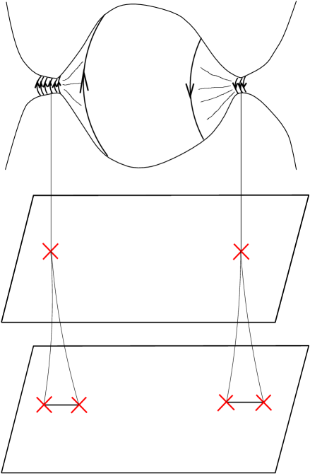
Figure 1: Depiction of the geometric transition from the open string picture with branes wrapped over minimal size $S^{2}$’s (top) to the large $N$ closed string dual where the branes and homologous $S^{2}$’s have been replaced by flux threading topologically distinct $S^{3}$’s of a new geometry (bottom).  The lines with red crosses denote finite length branch cuts on the Riemann surface of the local geometry after the transition.  In the open string picture the area of the $S^{2}$ in the middle of the bulge is approximately $|W^{\prime}(x)|$.  When branes are wrapped over these minimal size $S^{2}$’s, the bare tension of the branes creates a potential barrier against brane/anti-brane annihilation.

But as we increase the ’t Hooft coupling the $S^{3}$’s will expand in size so that higher order corrections to the effective potential will play a more important rôle in determining the vacuum of the theory.  These corrections are efficiently summarized by an auxiliary matrix model [19, 20, 21] which determines the classical periods of the closed string dual.  One of the purposes of this paper is to show that such corrections generate an intricate phase structure which is absent in the supersymmetric case.

When supersymmetry is broken, a metastable system of fluxes will eventually lower its energy by annihilating flux lines.  Rather than treating an individual system, it is therefore more appropriate to treat the totality of all possible flux configurations which admit metastable vacua.  To this end, we invert the question of finding critical points of $V_{\mathrm{eff}}$ and instead ask: Given a point in moduli space, which brane/anti-brane configurations would stabilize the moduli at this geometry?  Framing the question this way, we find necessary conditions for the existence of mutually non-supersymmetric metastable configurations of D5- and anti-D5-branes wrapped over the $S^{2}$’s of the original geometry.  We next analyze the phase structure of the two cut geometry.

Except when explicitly noted, the remainder of our results apply to the two cut geometry with the corresponding $S^{3}$’s supported by purely RR three form flux.  By determining the vacua of some special flux configurations, we argue that $N_{1}$, $N_{2}$ and $\theta_{\mathrm{YM}}$ respectively control the sizes and relative orientation of the cuts.  For $N_{1}=-N_{2}$ and $\theta_{\mathrm{YM}}$ arbitrary, we find metastable vacua such that the branch cuts are mirror reflections across an axis of the complex $x$-plane.   For $N_{1}$ and $N_{2}$ arbitrary and $\theta_{\mathrm{YM}}=0$, we find metastable vacua such that the branch cuts align along a common axis of the complex $x$-plane.

Even so, both supersymmetric and non-supersymmetric flux configurations admit many other potentially metastable vacua.  Indeed, even non-supersymmetric $U(N)$ Yang-Mills theory admits $O(N)$ metastable vacua which become exactly stable in the $N=\infty$ limit [22, 23].  Heuristically, these vacua are non-supersymmetric analogues of the $\mathrm{Tr}(-1)^{F}=N$ energetically degenerate supersymmetric confining vacua present in pure $\mathcal{N}=1$ $SU(N)$ super Yang-Mills theory [24].  For multi-cut geometries these other vacua are obtained at leading order in the closed string dual by rotating the branch cuts by a discrete angle $\pi/\left|N_{i}\right|$.  Although this geometric symmetry is deformed by higher order corrections, the corresponding supersymmetric confining vacua remain exactly degenerate in energy.

By contrast, we find that for non-supersymmetric confining vacua, the two loop contribution to the potential lifts this degeneracy so that it is energetically favorable for the branch cuts to align along a common axis.  This corresponds to an alignment of phases in the glueball fields.  Physically this follows from the fact that the potential energy due to the Coulomb attraction between the branes and anti-branes is lowest for such a configuration.  We find that the energy dependence of the vacuum as a function of $\theta_{\mathrm{YM}}$ agrees with the form expected in large $N$ gauge theories.  In addition, we also find a large number of potentially metastable vacua in accord with expectations from large $N$ arguments.  Indeed, although there is a single energetically preferred confining vacuum, the rate of decay to this lowest energy configuration is suppressed by large $N$ effects.  Thus, once we have established the existence of a single metastable brane/anti-brane configuration, general arguments from large $N$ gauge theories imply the presence of a large number of additional potentially metastable vacua.

Restricting further to the cases $N_{1}=-N_{2}$ and $\left|N_{1}\right|\gg\left|N_{2}\right|$ with the branch cuts aligned with the energetically preferred configuration along the real axis of the complex $x$-plane, we find that for sufficiently large ’t Hooft coupling, but far before the cuts touch, the theory undergoes a phase transition which lifts the metastable vacua present at weak coupling.  This is a novel phenomenon where strong coupling effects lead to a loss of stability in a classically metastable brane/anti-brane system.

Once the ’t Hooft coupling is large and metastability is lost, we can ask about the fate of the vacuum.  In order to address this, it is necessary to go beyond the regime where a perturbative computation of the potential is valid. Since we have the exact potential at large $N$, we can study this regime as well.  Using a combination of numerical and analytic arguments, we find that the dynamics of the fluxes drive the moduli to a configuration where the branch cuts nearly touch.  Close to this region in moduli space, a gas of nearly tensionless domain walls will typically cause the system to tunnel to a metastable vacuum of lower flux.  When this does not occur, the cuts can touch and additional light magnetic states condense.  In this case, we find that the resulting geometry is a non-Kähler manifold.

The organization of the rest of this paper is as follows.  In section 2 we establish notation and review the conjecture of [6] on the large $N$ dual of spacetime filling D5-branes and anti-D5-branes wrapped over $S^{2}$’s of a non-compact Calabi-Yau threefold.  In section 3 we derive necessary conditions for the existence of a metastable vacuum.  Beginning in section 4 we specialize to the two cut geometry and explain how the fluxes control the sizes and relative orientation of the branch cuts.  We next show in section 5 that a two loop effect lifts the degeneracy in energy between the confining vacua of the theory so that it is energetically favorable for the branch cuts (i.e. the phases of the glueball condensates) to align along a common axis.  In this same section we also find a large number of additional potentially metastable vacua and compare the $\theta_{YM}$ dependence of the vacuum energy density with general expectations from large $N$ gauge theories.  In section 6 we show that for sufficiently large ’t Hooft coupling, this two loop effect lifts the metastable vacua present near the semi-classical expansion point.  This causes the branch cuts to expand until they nearly touch.  Section 7 discusses the behavior of the system near this region of moduli space, and section 8 presents our conclusions and possible avenues of further investigation.

2 Geometrically Induced Metastability

In this section we set our notation and discuss in more detail the large $N$ dual description of the metastable brane/anti-brane configuration we shall study in this paper.  The open string description of our system consists of D5-branes and anti-D5-branes which fill Minkowski space and wrap $n$ minimal size $S^{2}$’s of a local Calabi-Yau threefold defined by the hypersurface:

$$y^{2}=W^{\prime}(x)^{2}+uv$$ (3)

where $x,y,u,v\in\mathbb{C}$ and $W^{\prime}(x)\equiv g(x-a_{1})\cdots(x-a_{n})$ is a degree $n$ polynomial.  Because the geometry is non-compact, the $a_{i}$ correspond to non-normalizable modes which determine the relative separation between the branes.  The minimal size $S^{2}$’s of the geometry are all homologous and are located at the points where $W^{\prime}(x)$ vanishes.  Indeed, at a generic point of the complex $x$-plane the area of an $S^{2}$ is given by the relation:

$$A(x)=\left(\left|W^{\prime}(x)\right|^{2}+\left|r\right|^{2}\right)^{1/2}$$ (4)

where $r$ denotes the size of the $S^{2}$ at $x=a_{i}$.  Because the branes and anti-branes preserve different supersymmetries, the corresponding system does not preserve any supersymmetry.  While there is no topological obstruction to the branes and anti-branes annihilating, the system is nevertheless geometrically metastable because the bare tension of the branes produces a potential barrier against the expansion of the branes.  See figure (1) for the local behavior of this configuration.

In the holographic dual description, the branes and anti-branes wrapping $n$ homologous $S^{2}$’s of the original geometry are replaced by fluxes threading the $n$ topologically distinct $S^{3}$’s of the new geometry.  The local Calabi-Yau threefold after the transition is defined by the equation:

$$y^{2}=W^{\prime}(x)^{2}+b_{n-1}x^{n-1}+\cdots+b_{0}+uv$$ (5)

where the $b_{i}$ correspond to the $n$ normalizable complex deformation parameters of the Calabi-Yau.  This complex equation defines a two-sheeted Riemann surface fibered over the $u$ and $v$ coordinates.  The $b_{i}$ split the double roots of $W^{\prime}(x)^{2}$, creating $n$ finite length branch cuts on the complex $x$-plane of the Riemann surface.  See figure (2) for a depiction of this geometry.

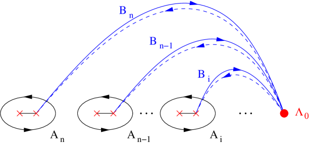
Figure 2: Depiction of the complex $x$-plane corresponding to the Riemann surface defined by equation (5) with $uv=0$.  The compact $A$-cycles reduce to counterclockwise contours which encircle each of the $n$ branch cuts of the Riemann surface.  The non-compact $B$-cycles reduce to contours which extend from $x=\Lambda_{0}$ on the lower sheet (dashed lines) to $x=\Lambda_{0}$ on the upper sheet (solid lines).

The $n$ $S^{3}$’s correspond to $n$ 3-cycles $A_{i}$ such that $A_{i}\cap A_{j}=0$ for all $i,j$.  Dual to each $A$-cycle is a non-compact $B$-cycle such that $A_{i}\cap B_{j}=-B_{j}\cap A_{i}=\delta_{ij}$ and $B_{i}\cap B_{j}=0$ for all $i,j$.  At the level of the Riemann surface, the $A_{i}$ reduce to $n$ distinct counter-clockwise contours encircling each of the $n$ branch cuts of the Riemann surface and the $B_{i}$ reduce to contours which extend from the point $x=\Lambda_{0}$ on the lower sheet to the point $x=\Lambda_{0}$ on the upper sheet.  The IR cutoff defined by $\Lambda_{0}$ in the geometry is identified with a UV cutoff in the open string description.  The periods of the holomorphic three form $\Omega$ along the cycles $A_{i}$ and $B_{i}$ define a basis of special coordinates for the complex structure moduli space:

$$S_{i}=\underset{A_{i}}{\int}\Omega,\text{ \ \ \ \ }\Pi_{i}=\text{\ }\frac{\partial\mathcal{F}_{0}}{\partial S_{i}}=\underset{B_{i}}{\int}\Omega$$ (6)

where $\mathcal{F}_{0}$ denotes the genus zero prepotential.  In the absence of fluxes, each $S_{i}$ corresponds to the scalar component of a $U(1)$ $\mathcal{N}=2$ vector multiplet.  Once branes are introduced, each $S_{i}$ is identified in the open string description with the size of a gaugino condensate.  Defining the period matrix:

$$\tau_{ij}=\frac{\partial\Pi_{i}}{\partial S_{j}}=\frac{\partial^{2}\mathcal{F}_{0}}{\partial S_{i}\partial S_{j}},$$ (7)

to leading order in the $1/N$ expansion, the Kähler metric for the effective field theory is $\operatorname{Im}\tau_{ij}$.  For future use we also introduce the Yukawa couplings:

$$\mathcal{F}_{ijk}\equiv\frac{\partial^{3}\mathcal{F}_{0}}{\partial S_{i}\partial S_{j}\partial S_{k}}.$$ (8)

We now describe the large $N$ dual description of brane configurations which preserve $\mathcal{N}=1$ supersymmetry.  To this end, recall that for supersymmetric flux configurations the flux-induced superpotential is [25]:

$$\mathcal{W}_{\mathrm{eff}}=\int H_{3}\wedge\Omega=\alpha\left(S_{1}+\cdots+S_{n}\right)+(N_{1}\Pi_{1}+\cdots+N_{n}\Pi_{n})$$ (9)

where $H_{3}$ denotes the net three form flux after the system undergoes a geometric transition:

$$H_{3}=H_{\mathrm{RR}}+\tau_{\mathrm{IIB}}H_{\mathrm{NS}}\text{.}$$ (10)

In the above equation, $H_{\mathrm{RR}}$ is the net RR three form field strength, $H_{\mathrm{NS}}$ is the net NS three form field strength and $\tau_{\mathrm{IIB}}=C_{0}+ie^{-\phi}$ is the type IIB axio-dilaton.  Explicitly,

$$N_{i}=\underset{A_{i}}{\int}H_{3},\text{ \ \ \ \ \ }\alpha=\alpha_{i}=-\underset{B_{i}}{\int}H_{3}$$ (11)

for all $i$.  Note in particular that when $N_{i}=p_{i}+\tau_{\mathrm{IIB}}q_{i}$ is a general complex number, this describes the geometric transition of a $(p_{i},q_{i})$ 5-brane wrapped over the $i^{\mathrm{th}}$ $S^{2}$ with $p_{i}$ units of D5-brane charge and $q_{i}$ units of NS5-brane charge. In the open string theory, the parameter $\alpha$ corresponds to minus the complexified gauge coupling evaluated at the UV cutoff:

$$\alpha=\alpha\left(\Lambda_{0}\right)=-\frac{\theta_{\mathrm{YM}}}{2\pi}-\frac{4\pi i}{g_{\mathrm{YM}}^{2}}.$$ (12)

The purely $S_{i}$ sector of the theory is described by the Lagrangian density:

$$\mathcal{L}_{S}=\frac{1}{g_{s}^{2}}\Lambda_{\mathrm{UV}}^{-4}\left(\operatorname{Im}\tau\right)_{i\overline{j}}\partial_{\mu}S^{i}\partial^{\mu}\overline{S^{j}}+\Lambda_{\mathrm{UV}}^{4}V_{\mathrm{eff}}\left(S_{i},\overline{S_{j}}\right)$$ (13)

where $\Lambda_{\mathrm{UV}}$ is a UV mass scale which is potentially different from $\Lambda_{0}$, and $V_{\mathrm{eff}}$ is given by:

$$V_{\mathrm{eff}}=\partial_{k}\mathcal{W}_{\mathrm{eff}}\left(\frac{1}{\operatorname{Im}\tau}\right)^{kl}\overline{\partial_{l}\mathcal{W}_{\mathrm{eff}}}=\left(\alpha_{k}+N^{k^{\prime}}\tau_{k^{\prime}k}\right)\left(\frac{1}{\operatorname{Im}\tau}\right)^{kl}\left(\overline{\alpha}_{l}+\overline{\tau}_{ll^{\prime}}\overline{N}^{l^{\prime}}\right)\text{.}$$ (14)

When it will not cause any confusion, we will work in units where $\Lambda_{\mathrm{UV}}$ is normalized to unity.

Having reviewed the large $N$ dual description for $\mathcal{N}=1$ brane configurations, we now describe the $\mathcal{N}=0$ analogue of this description when some of the branes are replaced by anti-branes.  In [6] it was conjectured that the form of the flux-induced effective potential for the $S_{i}$’s is essentially unchanged from the supersymmetric case.  To properly compare the energy of both branes and anti-branes simultaneously, it is appropriate to shift $V_{\mathrm{eff}}$ by a multiple of the bare tensions of the branes [6]:

$$V_{\mathrm{eff}}\mapsto V_{\mathrm{eff}}+\frac{8\pi}{g_{\mathrm{YM}}^{2}}\left(N_{1}+\cdots+N_{n}\right)\text{.}$$ (15)

2.1 Matrix Models and $V_{\mathrm{eff}}$

In this subsection we review the connection between matrix models and special geometry.  As originally proposed in [19], the genus zero prepotential of the geometry defined by equation (5) is exactly computed by the planar limit of a large $M$ auxiliary matrix model with partition function:

$$Z_{\mathrm{MM}}=\frac{1}{\mathrm{Vol}\left(U\left(M\right)\right)}\int d\Phi\exp\left(-\frac{1}{g_{s}}\text{{Tr}}W\left(\Phi\right)\right)$$ (16)

where $\Phi$ is a holomorphic $M\times M$ matrix and the above matrix integral should be understood as a contour integral.  The prepotential of the $n$-cut geometry near the semi-classical expansion point is given by expanding the eigenvalues of $\Phi$ about the $n$ critical points of the polynomial $W$.  The usual eigenvalue repulsion term of the matrix model causes these eigenvalues to fill the $n$ cuts of the geometry after the geometric transition.  With $M_{i}$ eigenvalues sitting at the $i^{\mathrm{th}}$ cut of the geometry, this matrix model may be recast as an $n$-matrix model of the form:

$$Z_{\mathrm{MM}}=\frac{1}{\underset{i=1}{\overset{n}{{\displaystyle\prod}}}\mathrm{Vol}\left(U\left(M_{i}\right)\right)}\int d\Phi_{1}\cdots d\Phi_{n}\exp\left(-\frac{1}{g_{s}}\underset{i=1}{\overset{n}{\sum}}{\mathrm{Tr}}W_{i}\left(\Phi_{i}\right)-\frac{1}{g_{s}}{\mathrm{Tr}}W_{\mathrm{int}}\left(\Phi_{1},\cdots,\Phi_{n}\right)\right)$$ (17)

in the obvious notation.  We caution the reader that the numbers $M_{i}$ are unrelated to the wrapping numbers of the branes.

The connection between the above matrix model and the special geometry of the Calabi-Yau threefold defined by equation (5) is obtained as follows.  The periods of the $A$-cycles are given by the partial ’t Hooft couplings of the matrix model [19]:

$$S_{i}=g_{s}M_{i}\text{.}$$ (18)

Evaluating $Z_{\mathrm{MM}}$ in the saddle point approximation, the planar limit of the free energy for the matrix model is identified with the genus zero prepotential for the complex structure moduli space of the Calabi-Yau threefold:

$$\mathcal{F}_{0}=\mathcal{F}_{\mathrm{measure}}+\mathcal{F}_{\mathrm{pert}}$$ (19)

where $\mathcal{F}_{\mathrm{measure}}$ corresponds to contributions from the $\mathrm{Vol}\left(U\left(M_{i}\right)\right)$ factors in the path-integral measure [26] and $\mathcal{F}_{\mathrm{pert}}$ corresponds to perturbative contributions from planar Feynman diagrams:

$$2\pi i\mathcal{F}_{\mathrm{measure}} =\underset{i=1}{\overset{n}{\sum}}\frac{1}{2}S_{i}^{2}\log\frac{S_{i}}{{\Lambda_{0}^{3}}}$$ (20)

$$2\pi i\mathcal{F}_{\mathrm{pert}} =-\underset{i=1}{\overset{n}{\sum}}S_{i}W(a_{i})+\underset{0\leq i_{1},\cdots,i_{n}}{\sum}C_{i_{1}\cdots i_{n}}S_{1}^{i_{1}}\cdots S_{n}^{i_{n}}\text{.}$$ (21)

From the perspective of the open string theory, the contribution $\mathcal{F}_{\mathrm{measure}}$ reproduces the expected Veneziano-Yankielowicz terms in the superpotential.  At leading order in the expansion of the periods about small $S_{i}$, these contributions serve to stabilize the magnitude of the glueball fields at the exponentially small value $\sim\exp\left(-8\pi^{2}/g_{\mathrm{YM}}^{2}\left|N_{i}\right|\right)$.  In addition to this leading order behavior, the power series in the $S_{i}$’s given by $\mathcal{F}_{\mathrm{pert}}$ produces subleading corrections to the form of the glueball potential.  Although the form of such corrections are difficult to calculate for a general confining gauge theory, in the present case the integrable structure of the matrix model ensures that the $C_{i_{1}...i_{n}}$ are in principle calculable.

2.2 Leading Order Behavior

Following [6], we now review the leading order behavior of metastable critical points of $V_{\mathrm{eff}}$ near the semi-classical expansion point.  Expanding the genus zero prepotential to quadratic order in the $S_{i}$’s, the period matrix is:

$$\tau_{ii}=\frac{1}{2\pi i}\log\frac{S_{i}}{W^{\prime\prime}(a_{i})\Lambda_{0}^{2}}\text{,\ \ \ \ \ \ }\tau_{ij}=\frac{-1}{2\pi i}\log\frac{\Lambda_{0}^{2}}{\Delta_{ij}^{2}}$$ (22)

for all $i\neq j$.  In the above expression $\Delta_{ij}=a_{i}-a_{j}$ is the relative separation between the minimal cycles over which branes or anti-branes wrap.  From the perspective of the auxiliary matrix model, this leading order behavior corresponds to the sum of the measure factor terms and all one loop planar diagrams.  These latter perturbative contributions give rise to terms in the prepotential proportional to $S_{i}S_{j}$.  See figure (3) for the one loop contributions to the prepotential of the two cut geometry.

Figure 3: Topologically distinct one loop planar diagram contributions to the prepotential for the two cut matrix model.  Solid lines denote branes and dashed lines denote anti-branes.

For sufficiently small $\left|N_{i}\right|$ the complex structure moduli are stabilized at exponentially small values [6]:

$$S_{N_{i}>0} =\zeta_{i}W^{\prime\prime}\left(a_{i}\right)\Lambda_{0}^{2}\underset{j\neq i}{\overset{N_{j}>0}{{\displaystyle\prod}}}\left(\frac{\Lambda_{0}}{\Delta_{ij}}\right)^{2\left|\frac{N_{j}}{N_{i}}\right|}\underset{k\neq i}{\overset{N_{k}<0}{{\displaystyle\prod}}}\left(\frac{\overline{\Lambda_{0}}}{\overline{\Delta_{ij}}}\right)^{2\left|\frac{N_{k}}{N_{i}}\right|}\exp\left(-\frac{2\pi i\alpha}{\left|N_{i}\right|}\right)$$ (23)

$$S_{N_{i}<0} =\zeta_{i}W^{\prime\prime}\left(a_{i}\right)\Lambda_{0}^{2}\underset{j\neq i}{\overset{N_{j}>0}{{\displaystyle\prod}}}\left(\frac{\overline{\Lambda_{0}}}{\overline{\Delta_{ij}}}\right)^{2\left|\frac{N_{j}}{N_{i}}\right|}\underset{k\neq i}{\overset{N_{k}<0}{{\displaystyle\prod}}}\left(\frac{\Lambda_{0}}{\Delta_{ij}}\right)^{2\left|\frac{N_{k}}{N_{i}}\right|}\exp\left(\frac{2\pi i\overline{\alpha}}{\left|N_{i}\right|}\right)$$ (24)

where $\zeta_{i}$ denotes an $N_{i}^{\mathrm{th}}$ root of unity.  As expected, there is a mass splitting at leading order between the bosons and fermions which explicitly demonstrates that supersymmetry is broken.  Finally, at leading order there is only a single critical point of the physical potential near the semi-classical expansion point corresponding to the metastable minimum.  See figure (4) for an example of this behavior in the two cut geometry.

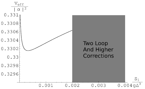
Figure 4: Plot of $V_{\mathrm{eff}}/\left|\alpha\right|^{2}$ in the one loop approximation along the locus $S_{1}/g\Delta^{3}=-S_{2}/g\Delta^{3}>0$ for a flux configuration with $N_{1}=-N_{2}$.  In this plot $\Lambda_{0}/\Delta\sim 10^{4}$ and $\left|N_{1}/\alpha\right|\sim 0.1$.  In the neighborhood of the semi-classical expansion point there is a single critical point which is metastable.

2.3 Two Loop Corrections

We now describe two loop corrections to $V_{\mathrm{eff}}$.  Figure (5) depicts the collection of topologically distinct diagrams which contribute to the cubic term of the genus zero prepotential.  Rather than describe the relative contribution of each of the twelve topologically distinct two loop planar diagrams, we merely give an example of the relevant combinatorics.  The combinatorial factors for the two diagrams with purely solid lines corresponding to the disk with two holes and two disks attached by a tube in figure (5) are respectively $1/6$ and $1/2$.  The remaining two loop contributions generate additional terms at cubic order in the genus zero prepotential and are computed in [27].

Figure 5: Two loop planar diagram contributions to the genus zero prepotential of the two cut geometry.  Solid lines denote branes and dashed lines denotes anti-branes.

3 Critical Points of $V_{\mathrm{eff}}$

In this section we derive necessary conditions that a flux configuration must satisfy in order for the flux induced effective potential:

$$V_{\mathrm{eff}}=\left(\alpha_{k}+N^{k^{\prime}}\tau_{k^{\prime}k}\right)\left(\frac{1}{\operatorname{Im}\tau}\right)^{kl}\left(\overline{\alpha}_{l}+\overline{\tau}_{ll^{\prime}}\overline{N}^{l^{\prime}}\right)$$ (25)

to possess a critical point.  Because such configurations are not absolutely stable, the amount of flux through each $A$-cycle will decrease over a sufficiently long time scale.  Rather than treating one particular metastable flux configuration, it is therefore more appropriate to treat the totality of all flux configurations which admit metastable vacua.  Indeed, we ask the inverse question: Given a point in moduli space, what configuration of fluxes would stabilize the moduli at this point?  To this end, we solve for the fluxes as a function of the critical point.

In what follows, we shall not require that the flux vector $N$ be an element of an integral lattice.  Indeed, because the critical points of the effective potential are invariant under an overall rescaling of $\alpha$ and the $N_{i}$, we may approximate the $N_{i}$ as continuous parameters once they have been rescaled to a sufficiently large value.  Further, we shall at first allow configurations with $N_{i}\in\mathbb{C}$.

The critical points are given by differentiating the effective potential with respect to the $S_{j}$ for $j=1,\cdots,n$:

$$0 =-2i\partial_{j}V_{\mathrm{eff}}=\left(\alpha+N\overline{\tau}\right)^{t}\frac{1}{\operatorname{Im}\tau}\left(\partial_{j}\tau\right)\frac{1}{\operatorname{Im}\tau}\left(\overline{\alpha}+\overline{\tau}\overline{N}\right)$$ (26)

$$\equiv W^{t}\left(\partial_{j}\tau\right)V$$ (27)

where we have introduced two n-component column vectors $V$ and $W$:

$$V =\frac{1}{\operatorname{Im}\tau}\left(\overline{\alpha}+\overline{\tau}\overline{N}\right)$$ (28)

$$W =\frac{1}{\operatorname{Im}\tau}\left(\alpha+\overline{\tau}N\right)$$ (29)

and for compactness we have suppressed all indices determined by matrix multiplication.  Solving for the n-component vectors $N$ and $\alpha$ in terms of $V$, $W$ and $\tau$ yields:

$$2iN =\overline{V}-W$$ (30)

$$2i\alpha =\tau W-\overline{\tau}\overline{V}.$$ (31)

It is therefore sufficient to express $V$ and $W$ as functions of the moduli.

Before proceeding to the solution of these equations, we now argue that for a given point in moduli space there are at most $2^{n}$ flux configurations such that this point is a critical point of $V_{\mathrm{eff}}$.  In addition to the $n$ conditions of equation (27), we obtain $n-1$ conditions from equation (31).  Indeed, because the column vector $\alpha$ is proportional to the vector with 1’s for all entries, the $n-1$ dimensional subspace orthogonal to $\alpha$ is independent of both the moduli and the fluxes.  Letting $T_{0},\cdots,T_{n-2}$ denote the $n-1$ independent vectors which span this subspace, the dot product of the $T_{i}$ with equation (31) yields an additional $n-1$ equations:

$$0=W^{t}\tau T_{i}-\overline{V}^{t}\overline{\tau}T_{i}$$ (32)

for $i=0,\cdots,n-2$.

Combining equations (27) and (32) yields a total of $2n-1$ complex equations for $2n$ complex variables.  Because the critical points are insensitive to the rescaling of the $n+1$ component row vector $\left(\alpha,N_{1},\cdots,N_{n}\right)$, we conclude that up to an overall rescaling by a complex number, there are a finite number of fluxes which satisfy the required conditions.  Finally, because the system consists of $n-1$ linear equations and $n$ quadratic equations, the number of “critical fluxes” at a given point in moduli space is at most $2^{n}$.

3.1 Non-Supersymmetric Solutions

We now restrict our attention to flux configurations which break supersymmetry.  In this case, the vectors $V$ and $W$ each have at least one non-zero component.  To isolate the projective nature of the solutions, we introduce affine versions of $V$ and $W$ which are completely fixed by the moduli dependent matrices $\tau$ and $\partial_{i}\tau$.  Without loss of generality, we may take the non-zero component of $V$ to be $V_{1}$ and that of $W$ to be $W_{n}$.  Now define rescaled $n$-component vectors $\nu$ and $\omega$ such that their complex conjugates satisfy:

$$V =V_{1}\overline{\nu}\equiv V_{1}\left|\overline{\nu}\right\rangle\text{ \ \ \ \ \ \ \ \ \ \ \ \ \ \ \ \ \ }V^{t}=V_{1}\left\langle\nu\right|$$ (33)

$$W =W_{n}\overline{\omega}\equiv W_{n}\left|\overline{\omega}\right\rangle\text{ \ \ \ \ \ \ \ \ \ \ \ \ \ }W^{t}=W_{n}\left\langle\omega\right|.$$ (34)

where to reduce notational clutter we have switched to bra and ket notation.  The $2n-2$ non-trivial components of $\nu$ and $\omega$ are therefore fixed as functions of the moduli by the $2n-2$ equations:

$$0 =\left\langle\omega\right|\partial_{j}\tau\left|\overline{\nu}\right\rangle$$ (35)

$$0 =\left\langle\omega\right|\tau\left|T_{0}\right\rangle\left\langle\overline{\nu}\right|\overline{\tau}\left|T_{k}\right\rangle-\left\langle\overline{\nu}\right|\overline{\tau}\left|T_{0}\right\rangle\left\langle\omega\right|\tau\left|T_{k}\right\rangle$$ (36)

where $j=1,\cdots,n$ and $k=1,\cdots,n-2$ with $N$ and $\alpha$ given by:

$$\frac{2i}{C}\left|N\right\rangle =\left|\nu\right\rangle\left\langle\omega\right|\tau\left|T_{0}\right\rangle-\left|\overline{\omega}\right\rangle\left\langle\overline{\nu}\right|\overline{\tau}\left|T_{0}\right\rangle$$ (37)

$$\frac{2i}{C}\left|\alpha\right\rangle =\tau\left|\overline{\omega}\right\rangle\left\langle\overline{\nu}\right|\overline{\tau}\left|T_{0}\right\rangle-\overline{\tau}\left|\nu\right\rangle\left\langle\omega\right|\tau\left|T_{0}\right\rangle$$ (38)

where $C$ is an non-zero complex constant which is undetermined by the equations.  Because the form of these equations is somewhat similar to those obtained in the study of the attractor equations of Calabi-Yau black holes [28, 29, 30, 31], we will loosely refer to the above as our attractor-like equations.

3.1.1 Brane Types and the Real Flux Locus

Our goal is to study the large $N$ dual description of a system of D5-branes and anti-D5-branes.  Note, however, that the attractor-like equations (37) and (38) indicate that every point in moduli space is a critical point of $V_{\mathrm{eff}}$ for some configuration of $N_{i}\in\mathbb{C}$.  To impose the additional requirement that the $N_{i}$ describe D5- and anti-D5-branes, we must further require that all of the ratios $N_{i}/N_{j}$ be real numbers.  This defines an $n+1$ real dimensional subspace inside the $2n$ real dimensional moduli space.

Although a complete characterization of the real flux locus is non-trivial, a partial description exists in the special case when the $n$ cuts of the geometry are all aligned along the real axis of the complex $x$-plane (so that the coefficients of the polynomial defining the Calabi-Yau threefold are all real) and with $\Lambda_{0}$ chosen so that the $\tau_{ij}$ are all purely imaginary.  We now show that in this case the ratios $N_{i}/N_{j}$ are all real and that $\theta_{\mathrm{YM}}=0$.  First note that there exists a finite neighborhood around the semi-classical expansion point such that $\tau_{ij}$ and $\mathcal{F}_{ijk}$ are pure imaginary.  Combining this with the leading order behavior of the $S_{i}$’s described in subsection 2.2, it follows that there exists a neighborhood around the semi-classical expansion point such that the operators $\left|\nu\right\rangle\left\langle\omega\right|$ and$\ \left|\overline{\omega}\right\rangle\left\langle\overline{\nu}\right|$ correspond to matrices with real entries.  By inspection of equations (37) and (38), this implies that $N_{i}/N_{j}$ is real and $\alpha/N_{i}$ is imaginary for all $i,j$.  Note that as expected, the $N_{i}$ control the sizes of the cuts and the parameter $\theta_{\mathrm{YM}}$ controls the relative orientation of the cuts in the geometry.

3.1.2 Example: Two Cut Geometry

With notation as in section 3.1, we have:

$$\left|T_{0}\right\rangle =\left[\begin{array}[c]{c}1\\ -1\end{array}\right],\text{ }\left|\nu\right\rangle=\left[\begin{array}[c]{c}1\\ \overline{V}_{2}/\overline{V_{1}}\end{array}\right],\text{ }\left|\omega\right\rangle=\left[\begin{array}[c]{c}\overline{W_{1}}/\overline{W_{2}}\\ 1\end{array}\right],$$ (45)

$$\left|\nu\right\rangle\left\langle\omega\right| =\left[\begin{array}[c]{cc}\rho_{w}&1\\ \overline{\rho_{v}}\rho_{w}&\overline{\rho_{v}}\end{array}\right],\text{ }\left|\overline{\omega}\right\rangle\left\langle\overline{\nu}\right|=\left[\begin{array}[c]{cc}\rho_{w}&\overline{\rho_{v}}\rho_{w}\\ 1&\overline{\rho_{v}}\end{array}\right]$$ (50)

where we have introduced:

$$\rho_{v} \equiv V_{2}/V_{1}=-\frac{d_{3}\pm\sqrt{d_{3}^{2}-4d_{1}d_{2}}}{2d_{2}}$$ (51)

$$\rho_{w} \equiv W_{1}/W_{2}=-\frac{d_{3}\pm\sqrt{d_{3}^{2}-4d_{1}d_{2}}}{2d_{1}}$$ (52)

with:

$$d_{1}=\det\left[\begin{array}[c]{cc}\mathcal{F}_{111}&\mathcal{F}_{112}\\ \mathcal{F}_{112}&\mathcal{F}_{221}\end{array}\right],\text{ }d_{2}=\det\left[\begin{array}[c]{cc}\mathcal{F}_{112}&\mathcal{F}_{221}\\ \mathcal{F}_{221}&\mathcal{F}_{222}\end{array}\right],\text{ }d_{3}=\det\left[\begin{array}[c]{cc}\mathcal{F}_{111}&\mathcal{F}_{112}\\ \mathcal{F}_{221}&\mathcal{F}_{222}\end{array}\right].$$ (53)

The $\pm$ signs of equations (51) and (52) are correlated.  The requirement that $g_{YM}^{2}>0$ leads to an unambiguous assignment of brane type for each branch.  Switching from the $+$ to the $-$ branch of equations (51) and (52) changes all branes (anti-branes) into anti-branes (branes).

4 Fluxes and Geometry

Unless explicitly noted, in the rest of this paper we restrict our analysis to the phase structure of the two cut geometry with the corresponding $S^{3}$’s supported by purely RR three form flux satisfying the condition $N_{1}/N_{2}<0$.  In this section we explain in more detail how $N_{1}$, $N_{2}$ and $\theta_{\mathrm{YM}}$ respectively control the sizes and relative orientation of the branch cuts.

Recall that the two cut geometry is given by the defining equation:

$$y^{2}=W^{\prime}(x)^{2}+b_{1}x+b_{0}+uv$$ (54)

where $W^{\prime}(x)=g(x-a_{1})(x-a_{2})$ and $b_{1}$ and $b_{0}$ control the sizes and orientations of the branch cuts by splitting the double roots $a_{i}$ to $a_{i}^{\pm}$.  When $uv=0$, this is the defining equation for an elliptic curve.  Without loss of generality, we may take the $a_{i}$ to be real numbers such that $a_{1}>a_{2}$.  When the cuts are small, we have [18]:

$$S_{1} \simeq\frac{g}{32}\left(a_{1}^{+}-a_{1}^{-}\right)^{2}\left(a_{1}^{+}+a_{1}^{-}-a_{2}^{+}-a_{2}^{-}\right)$$ (55)

$$-S_{2} \simeq\frac{g}{32}\left(a_{2}^{+}-a_{2}^{-}\right)^{2}\left(a_{1}^{+}+a_{1}^{-}-a_{2}^{+}-a_{2}^{-}\right)\text{.}$$ (56)

It thus follows that rotating the branch cuts in the complex $x$-plane changes the phases of the $S_{i}$’s.  Note that equations (55) and (56) are corrected at higher order by a real analytic power series in the $a_{i}^{\pm}$.  When $S_{1}>0>S_{2}$, the branch cuts of the geometry lie on the real axis of the $x$-plane.  Finally, for future use we set $\Delta=a_{1}-a_{2}$.

It follows from the discussion in subsection 3.1.1 that the space of critical points which satisfy the condition $N_{1}/N_{2}<0$ defines a three real dimensional subspace of the four real dimensional subspace locally described by the coordinates $S_{1}$ and $S_{2}$.

Although an exact characterization of this subspace is beyond our reach, we can still provide a crude sketch by considering various special limits.  At leading order in the expansion of the periods, the critical points of the effective potential for $N_{1}>0>N_{2}$ are [6]:

$$\frac{S_{1}}{g\Delta^{3}} =\zeta_{1}\left(\frac{\Lambda_{0}}{\Delta}\right)^{2}\left(\frac{\overline{\Lambda_{0}}}{\overline{\Delta}}\right)^{2\left|\frac{N_{2}}{N_{1}}\right|}\exp\left(\frac{2\pi i\alpha}{\left|N_{1}\right|}\right)\text{ \ \ \ \ \ }$$ (57)

$$-\frac{S_{2}}{g\Delta^{3}} =\zeta_{2}\left(\frac{\Lambda_{0}}{\Delta}\right)^{2}\left(\frac{\overline{\Lambda_{0}}}{\overline{\Delta}}\right)^{2\left|\frac{N_{1}}{N_{2}}\right|}\exp\left(-\frac{2\pi i\overline{\alpha}}{\left|N_{2}\right|}\right)$$ (58)

where the $\zeta_{i}$ are $N_{i}^{\mathrm{th}}$ roots of unity for $i=1,2$ and label the distinct confining vacua of the low energy theory.  Observe that $N_{1}$ and $N_{2}$ determine the magnitudes of $S_{1}$ and $S_{2}$.  The $N_{i}$ therefore determine the sizes of the branch cuts in the closed string dual.  Further, $\theta_{\mathrm{YM}}$ controls the relative phases of $S_{1}$ and $S_{2}$.  Indeed, as $\theta_{\mathrm{YM}}$ varies, the branch cuts rotate in opposite directions.  In this section we shall assume for simplicity that $\zeta_{1}=\zeta_{2}=1$.  This will necessarily limit the scope of our analysis.  We will return to this important point later on in section 5 where we will show that there is an energetically preferred confining vacuum corresponding to both of the branch cuts aligned along the real axis of the complex $x$-plane.

In the next two subsections we show that the flux configuration $N_{1}=-N_{2}$ admits metastable critical points on a $\mathbb{Z}_{2}$ symmetric locus in moduli space where $S_{1}=-\overline{S_{2}}$.  In this case the branch cuts are of equal size and are mirror reflections across the line halfway between $a_{1}$ and $a_{2}$.  We next show that flux configurations given by $N_{1}$, $N_{2}$ real and $\theta_{\mathrm{YM}}=0$ admit metastable critical points with $-S_{2},S_{1},\Lambda_{0}>0$.  In this case the branch cuts are of different sizes but are both aligned along the real axis of the $x$-plane.

4.1 Geometry of the $\mathbb{Z}_{2}$ Symmetric Locus

We now consider the geometry of the locus $S_{1}=-\overline{S_{2}}$.  Setting $uv=0$, the Riemann surface defined by equation (54) is invariant under the mapping $\sigma$:

$$x\mapsto-\overline{x},\text{ }y\mapsto-\overline{y}$$ (59)

provided that $g,b_{0},ib_{1}\in\mathbb{R}$, and $a_{1}=-\overline{a_{2}}$.

We show that invariance under this $\mathbb{Z}_{2}$ symmetry implies $S_{1}=-\overline{S_{2}}$.  The $S_{i}$’s reduce to line integrals on the Riemann surface:

$$S_{1}=\frac{1}{2\pi i}\underset{A_{1}}{{\displaystyle\oint}}ydx,\text{ \ \ \ \ \ }S_{2}=\frac{1}{2\pi i}\underset{A_{2}}{{\displaystyle\oint}}ydx$$ (60)

where by abuse of notation we let the $A_{i}$ also refer to the reduction of the $A$-cycles to two counterclockwise oriented closed loops encircling the two branch cuts of the geometry.  Whereas the differential element $y{d}x$ is by construction invariant under the map $\sigma$, the 1-cycles $A_{1}$ and $A_{2}$ transform as:

$$\sigma\left(A_{1}\right)=-A_{2},\text{ \ \ \ \ }\sigma\left(A_{2}\right)=-A_{1}.$$ (61)

It therefore follows that:

$$S_{1}+\overline{S_{2}}=0.$$ (62)

On the other hand, it follows from a general residue computation that [18]:

$$S_{1}+S_{2}=-\frac{1}{4g}b_{1}\text{.}$$ (63)

We therefore conclude that when $S_{1}=-S_{2}>0$, the branch cuts are of equal size and are aligned along the real axis of the $x$-plane.  More generally, $b_{0}$ (resp. $b_{1}$) predominantly controls the size (resp. relative orientation) of the branch cuts.

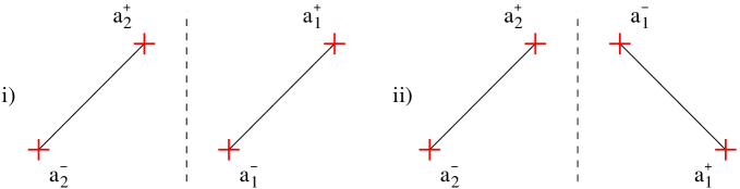
Figure 6: Depiction of the relative orientations of the branch cuts in the two cut geometry for: i) $S_{1}=-S_{2}$ and ii) $S_{1}=-\overline{S_{2}}$.

4.2 Flux Configurations of the $\mathbb{Z}_{2}$ Symmetric Locus

We now show that there exists a finite region in moduli space around the semi-classical expansion point such that the flux configuration $N_{1}=-N_{2}$ admits critical points satisfying $S_{1}=-\overline{S_{2}}$.  It follows from the explicit expressions for the $\tau_{ij}$ given in appendix A that near the semi-classical expansion point and along the locus $S_{1}=-\overline{S_{2}}$:

$$\left[\begin{array}[c]{cc}\overline{\tau_{11}}&\overline{\tau_{12}}\\ \overline{\tau_{12}}&\overline{\tau_{22}}\end{array}\right]=\left[\begin{array}[c]{cc}-\tau_{22}&-\tau_{12}\\ -\tau_{12}&-\tau_{11}\end{array}\right]-\frac{M-\overline{M}}{2\pi i}\left[\begin{array}[c]{cc}1&1\\ 1&1\end{array}\right]$$ (64)

where $M\equiv\log\left(\Lambda_{0}^{2}/\Delta^{2}\right)$ and:

$$\mathcal{F}_{111}=\overline{\mathcal{F}_{222}}\text{,\ \ \ \ }\mathcal{F}_{112}=\overline{\mathcal{F}_{122}}.$$ (65)

Note that the above relations do not require $\Lambda_{0}$ to be a real number.

We now apply the above relations in order to simplify the attractor-like equations (37) and (38).  Equation (65) implies that along this locus, the determinants of equation (53) satisfy $d_{1}=\overline{d_{2}}$ and $d_{3}=\overline{d_{3}}$ so that the discriminant $d_{3}^{2}-4d_{1}d_{2}$ is a real number.  It thus follows from the formulae in appendix A that near the semi-classical expansion point:

$$d_{3}^{2}-4d_{1}d_{2}>0\text{.}$$ (66)

This in turn implies:

$$\overline{\rho_{v}}=\rho_{w}\text{.}$$ (67)

Substituting equations (64) and (67) into the attractor-like equations (37) and (38) yields:

$$\frac{2i}{C^{\prime}}\left[\begin{array}[c]{c}N_{1}\\ N_{2}\end{array}\right] =\left(1-\rho_{w}\right)\left[\begin{array}[c]{c}1\\ -1\end{array}\right]$$ (72)

$$\frac{2i}{C^{\prime}}\alpha =\left(\tau_{22}+\tau_{12}+\rho_{w}(\tau_{11}+\tau_{12})+\frac{M-\overline{M}}{2\pi i}(1+\rho_{w})\right)$$ (73)

where $C^{\prime}$ is a common rescaling factor.  Hence, $N_{1}=-N_{2}$ and:

$$\frac{\alpha}{N_{1}}=\frac{1+\rho_{w}}{1-\rho_{w}}\left(\tau_{11}+\tau_{12}+\frac{M-\overline{M}}{2\pi i}\right)+\frac{\tau_{22}-\tau_{11}}{1-\rho_{w}}.$$ (74)

4.3 Flux Configurations of the Real Locus

When $S_{1}>0>S_{2}$, an argument similar to the one given in the previous subsection establishes that in a finite neighborhood of the semi-classical expansion point, both $\rho_{v}$ and $\rho_{w}$ of equation (51) and (52) are again real.  In this case $\overline{\tau_{ij}}=-\tau_{ij}-(M-\overline{M})/2\pi i$ and the attractor-like equations may be written as:

$$\frac{2i}{C}\left[\begin{array}[c]{c}N_{1}\\ N_{2}\end{array}\right] =\left[\begin{array}[c]{c}2\rho_{w}\left(\tau_{11}-\tau_{12}\right)+\left(1+\rho_{v}\rho_{w}\right)\left(\tau_{12}-\tau_{22}\right)\\ 2\rho_{v}\left(\tau_{12}-\tau_{22}\right)+\left(1+\rho_{v}\rho_{w}\right)\left(\tau_{11}-\tau_{12}\right)\end{array}\right]$$ (79)

$$\frac{2i}{C}\alpha =\left(\rho_{v}\rho_{w}-1\right)\det\tau+\frac{M-\overline{M}}{2\pi i}\left(1+\rho_{v}\right)\left(\tau_{12}-\tau_{22}+\rho_{w}\left(\tau_{11}-\tau_{12}\right)\right).$$ (80)

Because $\tau_{ij}-\tau_{12}$ is pure imaginary and $\rho_{v}$ and $\rho_{w}$ are purely real, we conclude that $N_{1}/N_{2}$ is purely real.  Further, when $M=\overline{M}$, the ratio $\alpha/N_{1}$ is pure imaginary.  We therefore conclude that for $\theta_{\mathrm{YM}}=0$ and $M=\overline{M}$, $V_{\mathrm{eff}}$ admits critical points corresponding to geometries with the branch cuts aligned along the real axis of the $x$-plane.

5 Confining Vacua and Glueball Phase Alignment

In this section we show that two loop corrections to our metastable brane/anti-brane system generate an energetically preferred confining vacuum.  In the closed string dual this preferred vacuum corresponds to a configuration where the branch cuts align along a common axis.  We next estimate the tunneling rate for glueball phase re-alignment and find the rate of decay to this lowest energy configuration is suppressed by large $N$ effects which can only be countered by an exponentially small glueball field.  Viewing our construction as imbedded inside a compact Calabi-Yau, string theory requires that $\theta_{\mathrm{YM}}$ be treated as a dynamical field.  We show that the same effect which lifts the degeneracy between the confining vacua generates a potential for $\theta_{\mathrm{YM}}$ which is consistent with general expectations from large $N$ gauge theories.

5.1 Degenerate Confining Vacua

It is well-known that pure super Yang-Mills theory with gauge group $SU(N)$ has $N$ confining vacua counted by the Witten index ${\mathrm{Tr}}\left(-1\right)^{F}=N$.  Indeed, the glueball field of the theory attains $N$ distinct values:

$$S=\zeta\Lambda^{3}$$ (81)

where $\zeta$ denotes an $N^{\mathrm{th}}$ root of unity and $\Lambda$ is the holomorphic scale of confinement for the gauge group $SU(N)$.

We now show that at leading order in the expansion of the periods, the confining vacua of the $n$ cut geometry are also energetically degenerate.  To this end, note that equation (22) implies that for $i\neq j$, $\tau_{ij}$ is constant.  The claimed degeneracy now follows because the critical points of $V_{\mathrm{eff}}$ are given by extremizing with respect to the variables $N_{i}\log\left(S_{i}/\left(W^{\prime\prime}(a_{i})\Lambda_{0}^{2}\right)\right)$ for all $i$.

But whereas the energy of each confining vacuum in the supersymmetric case is zero to all orders in an expansion of the periods, higher order corrections in the non-supersymmetric case should lift this degeneracy.  Indeed, our expectation is that the Coulomb attraction between branes and anti-branes will cause the branch cuts of the closed string dual to align in order to more efficiently annihilate flux lines.  We now confirm this in the case of the two cut geometry.

5.2 Higher Order Corrections in the Two Cut Geometry

At leading order, the energy density of the brane/anti-brane system is [6]:

$$E^{(0)}=\frac{8\pi}{g_{\mathrm{YM}}^{2}}\left(\left|N_{1}\right|+\left|N_{2}\right|\right)-\frac{2}{\pi}\left|N_{1}\right|\left|N_{2}\right|\log\left|\frac{\Lambda_{0}}{\Delta}\right|^{2}\text{.}$$ (82)

Because $E^{(0)}$ does not depend on the phases of the glueball fields, the confining vacua are energetically degenerate.

At higher order the effective potential takes the form:

$$V_{\mathrm{eff}}=V_{\mathrm{eff}}^{(0)}+V_{\mathrm{pert}}\text{.}$$ (83)

Incorporating the two loop correction to $\tau_{ij}$ given in appendix A lifts the degeneracy in energy densities:

$$E=E^{(0)}-\frac{10\left|N_{1}\right|\left|N_{2}\right|}{\pi}\left(t_{1}+\overline{t_{1}}+t_{2}+\overline{t_{2}}\right),$$ (84)

where $t_{1}\equiv S_{1}/(g\Delta^{3})$ and $t_{2}\equiv-S_{2}/(g\Delta^{3})$ are given by equations (57) and (58), respectively.  The confining vacuum with the lowest energy density is given by the configuration with $t_{1}$ and $t_{2}$ as close to being real positive numbers as possible.  Without loss of generality, the geometrical significance of this result can be seen when $\Delta>0$.  It now follows from equations (55) and (56) and the remarks below these equations that in this case the branch cuts are nearly aligned along the line joining $x=a_{1}$ and $x=a_{2}$.

5.3 Tunneling Rates

In the previous subsection we showed that the two loop contribution to $V_{\mathrm{eff}}$ lifts the degeneracy in energy density between the many confining vacua of the theory.  In this subsection we compute the tunneling rate for glueball phase re-alignment.  In particular, we find that in the strict $N_{i}=\infty$ limit with fixed confinement scale, these additional confining vacua become exactly stable.  For finite $N_{i}$, this leads to the presence of a large number of additional metastable vacua of the type generically present in large $N$ gauge theories [23, 24].  On the other hand, treating the glueball field as an exponentially suppressed quantity, we find that the corresponding tunneling rate increases.

In general, such tunneling events correspond to the nucleation of a bubble of vacuum with lower energy density inside the higher energy density vacuum.  Assuming that in the Euclidean continuation of Minkowski space that this bubble is an $O(4)$ symmetric configuration, the thin wall approximation of the tunneling rate is [32]:

$$\Gamma\sim\exp\left(-S_{bounce}\right)=\exp\left(-\frac{27\pi^{2}}{2}\frac{T^{4}}{\left(\Delta V\right)^{3}}\right)$$ (85)

where $T$ is the tension of the domain wall and $\Delta V$ is the change in energy density between the two vacua.

The domain wall solutions separating the confining vacua of the theory are given by wrapping D5-branes over the $A$-cycle threaded by positive flux and anti-D5-branes over the $A$-cycle threaded by negative flux.  We approximate the tension of such a domain wall using the supersymmetric analogue with $N_{1},N_{2}>0$:

$$T=\frac{1}{g_{s}}\left|\mathcal{W}_{\mathrm{eff}}(\zeta_{1}S_{1},\zeta_{2}S_{2})-\mathcal{W}_{\mathrm{eff}}(\zeta_{1}^{\prime}S_{1},\zeta_{2}^{\prime}S_{2})\right|$$ (86)

where $\zeta_{i}$ and $\zeta_{i}^{\prime}$ are $N_{i}^{\mathrm{th}}$ roots of unity and the $S_{i}$’s are evaluated at a supersymmetric critical point.  For simplicity, we now restrict our analysis to tunneling events which only rephase $S_{1}$.  The leading order $S_{1}$ dependence of $\Pi_{1}$ and $\Pi_{2}$ is:

$$2\pi i\Pi_{1} =S_{1}\left(\log\frac{S_{1}}{g\Delta\Lambda_{0}^{2}}-1\right)$$ (87)

$$2\pi i\Pi_{2} =S_{1}\log\frac{\Delta^{2}}{\Lambda_{0}^{2}}$$ (88)

The tension of the domain wall solution which interpolates between different discrete phase choices for $S_{1}$ is therefore:

$$T=\frac{1}{2\pi g_{s}}\left|N_{1}S_{1}\left(\zeta_{1}-\zeta_{1}^{\prime}\right)\right|=\frac{1}{\pi g_{s}}\left|N_{1}S_{1}\sin\frac{\pi\left(l-l^{\prime}\right)}{N_{1}}\right|.$$ (89)

where $\zeta_{1}=\exp\left(2\pi il/\left|N_{1}\right|\right)$ and $\zeta_{1}^{\prime}=\exp\left(2\pi il^{\prime}/\left|N_{1}\right|\right)$.  The change in energy density between the two vacua has norm:

$$\left|\Delta V\right|=\frac{20\left|N_{1}\right|\left|N_{2}\right|\left|t_{1}\right|}{\pi}\left|\cos\left(\frac{\widehat{\theta}+2\pi l}{\left|N_{1}\right|}\right)-\cos\left(\frac{\widehat{\theta}+2\pi l^{\prime}}{\left|N_{1}\right|}\right)\right|$$ (90)

where $\widehat{\theta}/\left|N_{1}\right|$ denotes the argument of $t_{1}$.

We now estimate the value of $T^{4}/\left(\Delta V\right)^{3}$ for different glueball phase alignment tunneling events.  In particular, we show that glueball phase alignment typically proceeds via a single large drop in energy density rather than a sequence of tunneling events with smaller drops in energy.  As it is irrelevant for the considerations to follow, we suppress all dependence on $\widehat{\theta}$ in the expressions to follow.

First consider the tunneling event from $l=N_{1}/2$ to $l^{\prime}=0$ corresponding to a single instanton process with the largest possible drop in energy density.  The bounce action is proportional to:

$$S_{N_{1}/2\rightarrow 0}\varpropto T^{4}/\left(\Delta V\right)^{3}=\frac{1}{40^{3}\pi}\frac{\left|N_{1}\right|}{\left|N_{2}\right|^{3}}\frac{\left|t_{1}\right|\left|g\Delta^{3}\right|^{4}}{g_{s}^{4}}\text{.}$$ (91)

Because the scaling of the $N_{i}$ and $g_{s}^{-1}$ in the large $N$ limit are all comparable, note that the corresponding bounce action scales as $N^{2}$ so that for finite $t_{1}$ this tunneling event is highly suppressed.  Note, however, that it is also natural to consider the limit in which $t_{1}$ is exponentially suppressed.  In this case the tunneling rate increases.

Next consider the tunneling process from the vacuum $l=N_{1}/2$ to $l^{\prime}=N_{1}/2-\delta$ for $\delta$ small compared to $N_{1}$.  In this case, the bounce action is proportional to:

$$S_{N_{1}/2\rightarrow N_{1}/2-\delta}\varpropto T^{4}/\left(\Delta V\right)^{3}=\frac{1}{40^{3}\pi^{3}}\left|\frac{N_{1}}{N_{2}}\right|^{3}\frac{\left|t_{1}\right|\left|g\Delta^{3}\right|^{4}}{\delta^{2}g_{s}^{4}}$$ (92)

which scales as $N^{4}$ in the large $N$ limit.  The tunneling rate for a small re-alignment in the glueball phase is therefore much smaller than that due to a large re-alignment in phase.

This conclusion is further supported by considering the tunneling process from a vacuum $l=\delta$ to $l^{\prime}=0$ where $\delta$ is again small compared to $\left|N_{1}\right|$.  In this case we find that the bounce action is given by the same expression as equation (92).  The decay rate due to rephasing $t_{1}$ is therefore:

$$\Gamma\sim\exp\left(-\frac{27}{2}\frac{1}{40^{3}\pi}\left|\frac{N_{1}}{N_{2}}\right|^{3}\frac{\left|t_{1}\right|\left|g\Delta^{3}\right|^{4}}{\delta^{2}g_{s}^{4}}\right)\text{.}$$ (93)

It therefore follows that as $\delta$ increases, the corresponding tunneling rate also increases.  Tuning the parameters of the theory so that $t_{1}$ remains fixed, note that when the ratio $\left|N_{1}/N_{2}\right|\gg$ $1$, the tunneling rate is suppressed.  Conversely, when the ratio $\left|N_{2}/N_{1}\right|\gg$ $1$, the tunneling rate is higher and the smaller cut aligns along the real axis on a shorter time scale.  Physically this corresponds to the fact that the orientation of a cut fluctuates less as the amount of flux passing through the corresponding $A$-cycle increases.

5.4 Axion Potential

As we have seen above, the two loop contribution to $V_{\mathrm{eff}}$ aligns the phases of the glueball fields.  It follows from string theory that upon imbedding our model in a compact Calabi-Yau threefold, $\theta_{\mathrm{YM}}$ must be treated as a dynamical field with potential given by equation (84) evaluated at the preferred confining vacuum.  The effective value of the $\theta$-angle on the branes and anti-branes follows from the relation:

$$S_{i}=\zeta_{i}\Lambda_{i}^{3}=\zeta_{i}\left|\Lambda_{i}\right|^{3}\exp\left(i\theta_{i}/\left|N_{i}\right|\right)$$ (94)

where $\zeta_{i}$ denotes an $\left|N_{i}\right|^{\text{th}}$ root of unity.

We now illustrate the form of the axion potential in the case $N_{1}=-N_{2}\equiv N$.  Equations (57) and (58) imply that for such flux configurations, the phase of $\Lambda_{0}/\Delta$ does not contribute to the phases of the $S_{i}$’s.  For simplicity, we further restrict to the case where $g\Delta^{3}$ is purely real.  In this case, the effective value of the $\theta$-angles for the branes and anti-branes satisfy $\theta_{1}=-\theta_{2}=$ $\theta_{\mathrm{YM}}$.  The energy now takes the form:

$$E=E^{(0)}-\frac{20N^{2}\left|t\right|}{\pi}\left(\cos\left(\frac{\theta_{\mathrm{YM}}+2\pi l}{N}\right)+\cos\left(\frac{\theta_{\mathrm{YM}}+2\pi l^{\prime}}{N}\right)\right)$$ (95)

where $t\equiv t_{1}=t_{2}$ and $l$ and $l^{\prime}$ are integers.  Evaluating $l$ and $l^{\prime}$ at the preferred confining vacuum configuration yields a potential for the axion:

$$V_{\mathrm{ax}}\left(\theta_{\mathrm{YM}}\right)=E^{(0)}-\frac{40N^{2}\left|t\right|}{\pi}\underset{l\in\mathbb{Z}}{\min}\left(\cos\left(\frac{\theta_{\mathrm{YM}}+2\pi l}{N}\right)\right)=E^{(0)}-\frac{40N^{2}\left|t\right|}{\pi}\cos\left(\frac{\theta_{\mathrm{YM}}}{N}\right)$$ (96)

where in the last equality we have assumed that $\theta_{\mathrm{YM}}\in\left[-\pi,\pi\right)$.  This potential has a minimum at $\theta_{\mathrm{YM}}=0$.  In the more general case where $\left|N_{1}\right|\neq\left|N_{2}\right|$ and both $\Delta$ and $g\Delta$ acquire complex phases, the minimum of $V_{\mathrm{ax}}$ will be shifted away from this value.  Naively, the requirement that the physics remain invariant under the substitution $\theta_{\mathrm{YM}}\rightarrow\theta_{\mathrm{YM}}+2\pi$ appears incompatible with the $\theta_{\mathrm{YM}}/N$ dependence of the final expression of equation (96).  That the physics does remain invariant follows from the first equality of equation (96).

In fact, this is a general issue in large $N$ gauge theories.  Recall that in large $N$ $U(N)$ pure Yang-Mills theory, the Lagrangian density is:

$$\mathcal{L}=-\frac{N}{4\lambda}Tr\left(F_{\mu\nu}F^{\mu\nu}\right)+\frac{\theta}{64\pi^{2}}\varepsilon^{\alpha\beta\mu\nu}Tr\left(F_{\alpha\beta}F_{\mu\nu}\right)$$ (97)

where $\lambda$ denotes the ’t Hooft coupling of the theory.  The dependence of the vacuum energy density on the $\theta$-angle is:

$$E_{vac}\left(\theta\right)=N^{2}f\left(\frac{\theta}{N}\right)$$ (98)

where $f$ is a function which is well-defined in the large $N$ limit.  The factor of $N^{2}$ arises from the number of degrees of freedom and the $\theta/N$ dependence follows from the requirement that the energy density must possess a well-defined large $N$ limit [33, 22, 23].   In order to restore invariance under $\theta\rightarrow\theta+2\pi$, it is natural to conjecture that the full $\theta$ dependence of $E_{vac}$ is [22]:

$$E_{vac}\left(\theta\right)=N^{2}\underset{l\in\mathbb{Z}}{\min}f\left(\frac{\theta+2\pi l}{N}\right)$$ (99)

where the integers $l$ label distinct metastable branches of vacua.  It has been shown that this type of vacuum structure arises both in softly broken supersymmetric QCD with small gaugino masses [34, 35] as well as from D-brane constructions of large $N$ gauge theories [23].  In the limit $N=\infty$, it is expected that if $t_{1}$ remains fixed and in particular is not exponentially suppressed, that these additional vacua become exactly stable [23, 24].  This is indeed consistent with the decay rates given by equations (91), (92) and (93).  Multiple branches of vacua may also be present in QCD [36, 37, 38, 39, 40].

Returning to the first equality of equation (96), note that our expression for the vacuum energy density is of precisely the form conjectured in equation (99).  This provides an exactly calculable example where the expectations discussed above are explicitly borne out.  Indeed, although there are higher order corrections to $E_{vac}$ and therefore to $V_{\mathrm{ax}}$, to leading order in $1/N$, all of these corrections are captured by the closed string dual description.

6 Breakdown of Metastability

When the amount of flux through each $S^{3}$ is sufficiently low, the corresponding glueball field is stabilized at a small value.  But as shown in section 5, two loop contributions to $V_{\mathrm{eff}}$  generate a preferred confining vacuum which aligns the phases of the glueball fields.  In this section we show that for sufficiently large values of the ’t Hooft coupling, this same two loop effect lifts the metastable vacua present at weak coupling.  Note in particular that because the corrections to the Kähler potential are of order $1/N$, the holographic dual description of the brane dynamics in terms of the flux induced potential $V_{\mathrm{eff}}$ becomes more accurate as the amount of flux through each $S^{3}$ increases.

Before proceeding with a more precise analysis, we first give a heuristic derivation of the value of the ’t Hooft coupling for which we expect higher order corrections to $V_{\mathrm{eff}}$ to lift the metastable vacua present at weak coupling.  Recall from equation (82) that the leading order energy density of the brane/anti-brane system is:

$$E^{(0)}=\frac{8\pi}{g_{\mathrm{YM}}^{2}}\left(\left|N_{1}\right|+\left|N_{2}\right|\right)-\frac{2}{\pi}\left|N_{1}\right|\left|N_{2}\right|\log\left|\frac{\Lambda_{0}}{\Delta}\right|^{2}\text{.}$$ (100)

The first term corresponds to the bare tension of the branes and the second term corresponds to the Coulomb attraction between the branes.

Returning to the discussion near equation (15), it follows that when $\left|N_{1}\right|\gtrsim\left|N_{2}\right|$ and $N_{1}>0>N_{2}$, we have:

$$E^{(0)}\geq\frac{8\pi}{g_{\mathrm{YM}}^{2}}\left(N_{1}+N_{2}\right)$$ (101)

with similar inequalities for different choices of relative magnitudes and signs for the $N_{i}$.  We expect to lose metastability precisely when the Coulomb attraction contribution to the energy density becomes comparable to the bare tension of the branes.  This is near the regime where $E^{(0)}$ is close to saturating inequality (101).  This yields the following estimate for the breakdown of metastability:

$$\frac{1}{g_{\mathrm{YM}}^{2}\left|N_{1}\right|}\sim\log\left|\frac{\Lambda_{0}}{\Delta}\right|^{2}$$ (102)

where in the above expression we have dropped all factors of order unity.

Perhaps more surprisingly, this breakdown in metastability is calculable near the semi-classical expansion point.  Indeed, for illustrative purposes we show in the subsection to follow that for $N_{1}=-N_{2}$, the two loop contribution to the glueball potential causes $V_{\mathrm{eff}}$ to develop a local maximum.  Beyond this local maximum the potential subsequently rolls downward beyond the regime where perturbations about the semi-classical expansion point provide an accurate description.

The rest of this section is organized as follows.  For simplicity and with the analysis of section 5 in mind, we restrict to flux configurations which produce metastable vacua with the branch cuts aligned along the real axis of the complex $x$-plane.  In subsection 6.1 we illustrate in the case $N_{1}=-N_{2}$ that the two loop contribution to $V_{\mathrm{eff}}$ generates a local maximum for the glueball potential.  In subsection 6.2 we study the breakdown in metastability for flux configurations with $N_{1}=-N_{2}$ and $\theta_{\mathrm{YM}}=0$, and in subsection 6.3 we perform a similar analysis for the case $\left|N_{1}\right|\gg\left|N_{2}\right|$ and $\theta_{\mathrm{YM}}=0$.  In both cases we find that the value of the flux at which metastability breaks down is in rough agreement with the estimate given by equation (102).

6.1 Two Loop Corrections to $V_{\mathrm{eff}}$

In this subsection we show that the higher order corrections to the periods alter the shape of the flux induced effective potential.  Along the locus $S_{1}=-S_{2}>0$, the leading order behavior of the effective potential is:

$$V_{\mathrm{eff}}^{(0)}=\frac{\left|\alpha\right|^{2}}{\pi\left(2M-\log t\right)}\left(4\pi^{2}-\left|\frac{N}{\alpha}\right|^{2}\left(2M-\log t\right)\log t\right)$$ (103)

where we have introduced the parameter $t\equiv S_{1}/g\Delta^{3}=-S_{2}/g\Delta^{3}$.  This potential possesses a single extremum which is a minimum.  We now show that this behavior is only correct for very small $t$.  The higher order behavior of $V_{\mathrm{eff}}$ is:

$$V_{\mathrm{eff}}=\frac{\left|\alpha\right|^{2}}{\pi\left(2M+6t-\log t\right)}\left(\begin{array}[c]{c}4\pi^{2}-\left|\frac{N}{\alpha}\right|^{2}\left(2M-\log t\right)\log t\\ -\left|\frac{N}{\alpha}\right|^{2}\left(68Mt+204t^{2}+28t\log t\right)\end{array}\right).$$ (104)

To determine the appearance of a local maximum in $V_{\mathrm{eff}}$, we compare the relative $t$ dependence of all terms in the above expression.  The appearance of a local maximum is due to the term proportional to $68Mt$.  We may therefore approximate $V_{\mathrm{eff}}$ as:

$$V_{\mathrm{eff}} \simeq V_{\mathrm{eff}}^{(0)}-\frac{68M\left|N\right|^{2}}{\pi}\frac{t}{2M-\log t}$$ (105)

$$\equiv V_{\mathrm{eff}}^{(0)}+V^{(2)}\text{.}$$ (106)

We now show that for a suitable range of values, this new term causes $V_{\mathrm{eff}}$ to develop a local maximum and a local minimum.

To this end, first consider the derivative of $V_{\mathrm{eff}}^{(0)}$ with respect to $t$:

$$\frac{dV_{\mathrm{eff}}^{(0)}}{dt}\simeq\frac{\left|\alpha\right|^{2}}{\pi t(2M-\log t)^{2}}\left(-4M^{2}\left|\frac{N}{\alpha}\right|^{2}+4\pi^{2}+4M\left|\frac{N}{\alpha}\right|^{2}\log t-\left|\frac{N}{\alpha}\right|^{2}(\log t)^{2}\right).$$ (107)

Note that the term in parentheses is a quadratic polynomial in $\log t$ and therefore achieves a maximal value.  By including the contribution from $dV^{(2)}/dt$, we find that for suitable values of $\left|N/\alpha\right|$, the equation $dV_{\mathrm{eff}}/dt=0$ possesses at least two solutions.  These solutions correspond to a metastable minimum and a nearby maximum for the effective potential.

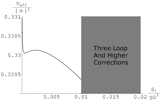
Figure 7: Plot of $V_{\mathrm{eff}}/\left|\alpha\right|^{2}$ in the two loop approximation along the locus $S_{1}/g\Delta^{3}=-S_{2}/g\Delta^{3}>0$ for a flux configuration with $N_{1}=-N_{2}$.  In this plot $\Lambda_{0}/\Delta\sim 10^{4}$ and $\left|N_{1}/\alpha\right|\sim 0.1$.

6.2 Breakdown of Metastability: $N_{1}=-N_{2}$

When $N_{1}=-N_{2}\equiv N$ and $\theta_{\mathrm{YM}}=0$, the metastable minima of $V_{\mathrm{eff}}$ correspond to two equal size branch cuts aligned along the real axis of the complex $x$-plane.  To study the appearance of an instability in $V_{\mathrm{eff}}$, we return to our general approach of solving for the fluxes as a function of moduli.  The only non-trivial moduli dependence arises from the ratio:

$$\frac{\alpha}{N}=-\frac{4\pi i}{g_{\mathrm{YM}}^{2}N}.$$ (108)

Along the locus $S_{1}=-S_{2}>0$, the moduli dependent function $\alpha/N$ may assume the same value multiple times.  This implies that for a given set of fluxes, there are multiple critical points of $V_{\mathrm{eff}}$.

We now briefly switch perspectives and view these critical points as functions of $\alpha/N$.  When these critical points approach the same point in moduli space, the effective potential develops a flat direction.  Viewed as a function of moduli, when the ’t Hooft parameter:

$$\lambda\equiv g_{\mathrm{YM}}^{2}\left|N\right|$$ (109)

reaches a maximal value, the system develops an instability.

We now determine the value of $t$ for which $\lambda$ attains a maximum.  It follows from equation (74) and the expressions of appendix A that:

$$\frac{8\pi^{2}}{\lambda}=-\log t+M+\overline{M}+t(6+20M+20\overline{M}-10\log t^{2})+O(t^{2}\log t)\text{.}$$ (110)

Note that to leading order in $t$, $\lambda^{-1}\sim$ $-\log t+M+\overline{M}$ and therefore does not possess a minimum.  The quantity $\lambda^{-1}$ is minimized when:

$$t_{\ast}=-\frac{1}{20W_{-1}\left(-e^{-L}\right)}$$ (111)

where $L\equiv\log\left|\Lambda_{0}^{4}/\Delta^{4}\right|+\log\left(20e^{-7/10}\right)$ and $W_{-1}$ is the $-1^{\mathrm{th}}$ branch of the Lambert W-function.

It is also of interest to study the $\Delta$ dependence of $t_{\ast}$.  For sufficiently small $t_{\ast}$ and $\Delta$, we have:

$$\log\left|\frac{\Lambda_{0}}{\Delta}\right|^{4}\simeq\frac{1}{20t_{\ast}}\text{.}$$ (112)

Fixing the value of $t$, we conclude that the system always develops an instability once $\Delta$ is sufficiently small.  In particular, we see that by tuning $\Delta$ to a sufficiently small value, $t_{\ast}$ can be made arbitrarily small, justifying the two loop approximation.

To conclude this subsection we estimate the value of $g_{\mathrm{YM}}^{2}\left|N\right|$ for which $V_{\mathrm{eff}}$ develops an instability.  It follows from equations (110) and (112) that for sufficiently small $\Delta$ and $t_{\ast}$:

$$\exp\left(\frac{8\pi^{2}}{\lambda_{\ast}}\right)=20\left|\frac{\Lambda_{0}}{\Delta}\right|^{4}\log\left|\frac{\Lambda_{0}}{\Delta}\right|^{4}$$ (113)

where $\lambda_{\ast}$ is the value of the bare ’t Hooft coupling at the phase transition.  If we now drop the factors $20$ and $\log\left|\frac{\Lambda_{0}}{\Delta}\right|^{4}$ in the above expression, we obtain:

$$\frac{1}{\lambda_{\ast}}\sim\frac{1}{4\pi^{2}}\log\left|\frac{\Lambda_{0}}{\Delta}\right|^{2}$$ (114)

up to factors of order unity.  This is in agreement with the analysis leading to equation (102).  Even so, equation (114) should be viewed as a crude upper bound.

6.2.1 Masses and the Mode of Instability: $N_{1}=-N_{2}$

Although the above analysis establishes that $V_{\mathrm{eff}}$ develops an instability for sufficiently large values of the flux, it does not directly indicate the mode of instability.  It also does not address whether additional modes of instability appear before reaching such a flux configuration.  We now show that all the other modes are stable up to this point and that the unstable mode of the system corresponds to the cuts remaining equal in size and expanding towards each other.  To establish this, we now compute the bosonic mass spectrum for fluxes close to the value where we expect to lose metastability.  After canonically normalizing the kinetic terms of $S_{1}$ and $S_{2}$ and expanding $V_{\mathrm{eff}}$ to quadratic order, the masses squared are:

$$m_{{RA}}^{2} =\frac{a^{2}}{1-v}+2a\left|N\right|\left(-\frac{10}{1+\sqrt{v}}+\frac{7}{(1-v)\pi\operatorname{Im}\tau_{11}}\right)$$ (115)

$$m_{{RS}}^{2} =\frac{a^{2}}{1-v}+2a\left|N\right|\left(-\frac{10}{1-\sqrt{v}}+\frac{7}{(1-v)\pi\operatorname{Im}\tau_{11}}\right)$$ (116)

$$m_{{IS}}^{2} =\frac{a^{2}}{\left(1+\sqrt{v}\right)^{2}}+2a\left|N\right|\left(\frac{10}{1+\sqrt{v}}+\frac{-3}{\left(1+\sqrt{v}\right)^{2}\pi\operatorname{Im}\tau_{11}}\right)$$ (117)

$$m_{{IA}}^{2} =\frac{a^{2}}{\left(1-\sqrt{v}\right)^{2}}+2a\left|N\right|\left(\frac{10}{1-\sqrt{v}}+\frac{17}{\left(1-\sqrt{v}\right)^{2}\pi\operatorname{Im}\tau_{11}}\right)$$ (118)

where in the above, $RA$ denotes the real anti-symmetric mode corresponding to both $S_{i}$’s real with one cut growing while the other shrinks, $RS$ denotes the real symmetric mode corresponding to both $S_{i}$’s real with both cuts growing in size together, and $IS$ and $IA$ are similarly defined for the imaginary components of the $S_{i}$’s.  Further, we have introduced the parameters:

$$a=\frac{|N|}{2\pi t\operatorname{Im}{\tau}_{11}}\text{, }v=\frac{\operatorname{Im}{{\tau}_{12}}^{2}}{\operatorname{Im}{\tau}_{11}\operatorname{Im}{\tau}_{22}}$$ (119)

where all moduli dependent functions are explicitly evaluated at the critical point determined by the ’t Hooft coupling $\lambda$.  In equations (115-118), the term proportional to $a^{2}$ corresponds to the leading order contribution to the masses squared computed in [6], and the term proportional to $2a\left|N\right|$ corresponds to the two loop correction to this value.  As expected based on general symmetry arguments, we find that as a function of $\left|N/\alpha\right|$, $m_{RS}^{2}$ approaches zero as the flux approaches the value given by equation (114).  In figure (8) we show the behavior of $m_{RS}^{2}$ and the next smallest mass squared $m_{IS}^{2}$ as a function of $\left|N/\alpha\right|$ near the regime where metastability is lost.

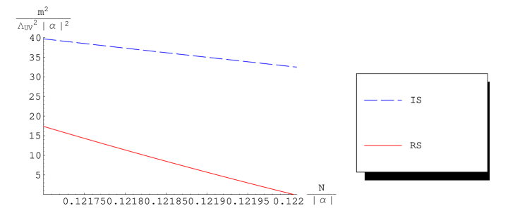
Figure 8: Plot of the two smallest masses $m_{RS}^{2}$ and $m_{IS}^{2}$ as a function of $\left|N/\alpha\right|$ for $\Lambda_{0}/\Delta\sim 10^{4}$.  At a value of $\left|N/\alpha\right|\sim 0.122$ the system develops an instability.  This value is in rough agreement with the estimate of equation (114).

It is also of interest to consider the difference in masses between the bosonic and fermionic fluctuations dictated by the underlying $\mathcal{N}=2$ structure of the theory.  We find that the masses of the fermions naturally group into two sets of values.  At leading order in $1/N$, the $\mathcal{N}=2$ supersymmetry of the theory is spontaneously broken.  This indicates the presence of two massless goldstinos.  Labeling the fermionic counterparts of the gauge bosons and the $S_{i}$’s respectively by $\psi_{A}^{(i)}$ and $\psi_{S}^{(i)}$, we find that when $N_{1}=-N_{2}$, the non-zero masses of the canonically normalized fermionic fields are all equal and given by the value:

$$|m_{\psi}|=\frac{a}{\left(1-v\right)}+\left|N\right|\frac{7+10\sqrt{v}}{1-v}$$ (120)

where as before, the first term corresponds to the leading order mass and the second term is the two loop correction to this value.  In figure (9) we compare the masses squared of the bosonic and fermionic fluctuations.

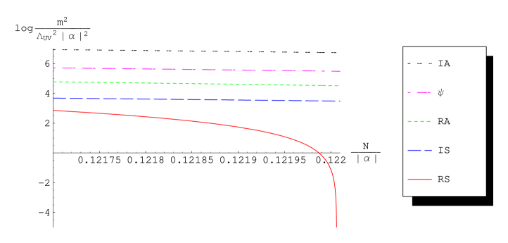
Figure 9: Plot of $\log(m^{2}/(\left|\alpha\right|^{2}\Lambda_{UV}^{2}))$ as a function of $\left|N/\alpha\right|$ for $\Lambda_{0}/\Delta\sim 10^{4}$.   The bosonic and fermionic masses squared are given by equations (115-118) and (120), respectively.

Although we do not include the details here, we find more generally that for vacua which satisfy $S_{1}=-\overline{S_{2}}$, the system develops an instability at a similar value of $\left|N/\alpha\right|$.  In this case, the mode of instability causes the cuts to expand in size and rotate towards the real axis of the complex $x$-plane.  This is in agreement with the physical expectation that the flux lines annihilate most efficiently when the branch cuts are aligned along the real axis of the complex $x$-plane.

6.3 Breakdown of Metastability: $\left|N_{1}\right|\gg\left|N_{2}\right|$

We now study the behavior of $V_{\mathrm{eff}}$ for flux configurations with $\left|N_{1}\right|\gg\left|N_{2}\right|$ and $\theta_{\mathrm{YM}}=0$.  More precisely, we also take $N_{1}$ small enough so that the two loop approximation of $V_{\mathrm{eff}}$ is valid.  In this case, the modulus $t_{1}\equiv S_{1}/g\Delta^{3}$ fluctuates much less than $t_{2}\equiv-S_{2}/g\Delta^{3}$.  Further, because the behavior of $V_{\mathrm{eff}}$ is relatively insensitive to the value of $\alpha/N_{2}$, it is sufficient to fix $\alpha/N_{2}$ and determine the value of $\alpha/N_{1}$ for which $V_{\mathrm{eff}}$ develops a flat direction.

To this end, we employ a strategy similar to that of subsection 6.2 and use the attractor-like equations to treat $\alpha/N_{1}$ as a function of the single modulus $t_{2}$.  Because a larger amount of flux passes through the $S^{3}$ corresponding to $t_{1}$, it is enough to expand $\alpha/N_{1}$ to first order in $t_{1}$ and to leading order in $\log t_{2}$.  Extremizing $\alpha/N_{1}$ with respect to $t_{2}$, we find that $V_{\mathrm{eff}}$ develops a flat direction when:

$$\frac{8\pi^{2}}{g_{\mathrm{YM}}^{2}\left|N_{1}\right|}\simeq\frac{M}{80t_{1}}\text{.}$$ (121)

Using equation (57) to approximate the value of $t_{1}$ yields the value of $\lambda_{1}\equiv g_{\mathrm{YM}}^{2}\left|N_{1}\right|$ for which the system develops an instability:

$$\frac{1}{\lambda_{1,\ast}}\simeq-\frac{1}{8\pi^{2}}W_{-1}\left(-\frac{1}{80}\frac{\log\left|\frac{\Lambda_{0}}{\Delta}\right|^{2}}{\left|\frac{\Lambda_{0}}{\Delta}\right|^{2}}\right)$$ (122)

where $\lambda_{1,\ast}$ denotes the bare ’t Hooft coupling at the phase transition.  To obtain a crude estimate of when we expect to lose metastability, we treat the left hand side of equation (121) as an order one number, obtaining:

$$\frac{1}{\lambda_{1,\ast}}\sim\frac{1}{8\pi^{2}}\log\left|\frac{\Lambda_{0}}{\Delta}\right|^{2}\text{.}$$ (123)

This estimate is in accord with equation (102).

As in subsection 6.2, it is important to compute the masses squared of the bosonic fluctuations at the metastable minimum in order to determine the mode of instability for this flux configuration.  In this case, the appropriate linear combination of fields which diagonalizes the mass matrix is somewhat messier and we defer the details of this computation to appendix B.  We find that the unstable mode corresponds to the smaller branch cut increasing in size at a much faster rate than its larger counterpart.

7 Endpoints of a Phase Transition

For sufficiently large ’t Hooft coupling, the metastable vacua present at weak coupling cease to exist.  The moduli subsequently roll to larger values so that a perturbative expansion in the glueball fields $S_{i}$ is no longer valid.  As the branch cuts increase in size and meet each other, the 3-cycle $B_{1}-B_{2}$ reduces to zero size.  We have checked numerically that over this range the potential attains a minimal value only once the cuts touch.  Because no flux passes through $B_{1}-B_{2}$, the moduli will not be stabilized away from the corresponding conifold point.  Near this region, the contribution of new light states associated to a D3-brane wrapping $B_{1}-B_{2}$ and an instanton gas of D5-branes all wrapping the same cycle will determine the low energy dynamics of the theory.

Let us first consider the contribution due to the D5-branes.  From the perspective of the spacetime, a D5-brane wrapping $B_{1}-B_{2}$ corresponds to a domain wall solution which separates vacua with distinct values of the flux.  Indeed, for vacua near the semi-classical expansion point, this is the primary mechanism by which the vacuum can decay to a supersymmetric flux configuration [6].  As $B_{1}-B_{2}$ collapses, the corresponding action for quantum tunneling tends to zero and a gas of D5-branes will scan over all available flux configurations.  This will necessarily change the shape of the potential for the moduli.  When enough flux has been annihilated, it is then possible for the moduli to subsequently either quantum mechanically tunnel through moduli space or (if the shape of the potential has changed enough) classically roll back out to the semi-classical regime.  Letting the vector $\overrightarrow{N_{\ast}}$ denote the critical value of the fluxes for which metastability is lost, the flux vector for the new metastable minimum will differ from $\overrightarrow{N_{\ast}}$ by a finite amount.

Next consider the contribution due to the D3-brane.  As the 3-cycle $B_{1}-B_{2}$ collapses, the geometry approaches a conifold point such that both the Kähler metric and $V_{\mathrm{eff}}$ develop singularities.  Just as in the supersymmetric case, the additional light states which resolve this singularity correspond to a D3-brane wrapped over $B_{1}-B_{2}$.  Because an analysis of a generic flux configuration would require a fairly precise knowledge of the periods near this region in moduli space, we restrict our discussion to the case $N_{1}=-N_{2}$ with the branch cuts aligned along the real axis of the complex $x$-plane.  In subsection 7.4 we present evidence that if we ignore the presence of nearly tensionless domain walls, the light magnetic states of the D3-brane condense and cause such a flux configuration to transition to a non-Kähler manifold.

The rather different physical nature of the D5-brane instanton gas and massless states contributed by the D3-brane indicate that a more detailed analysis of the endpoint of this phase transition is likely to be quite difficult.  Our general expectation, however, is that the contribution due to the D5-branes will typically cause the moduli to relax back to the semi-classical expansion point.  Indeed, in the case $\left|N_{1}\right|\gg\left|N_{2}\right|$, the $N_{2}$ units of flux can be treated as a probe of the background flux configuration determined by $N_{1}$.  In this case it is doubtful that such a small perturbation could cause the geometry to undergo a transition to a non-Kähler manifold.

The situation is less clear when $N_{1}\sim-N_{2}$.  As we show in subsection 7.1, when $N_{1}=-N_{2}\equiv N$ and along the locus $S_{1}=-S_{2}>0$, the value of the potential when the cuts touch is independent of $N$.  This implies that while the gas of tensionless domain walls can still drive the system back to a metastable vacuum, it is not energetically favorable to eliminate a small amount of flux.  The additional light magnetic states due to the D3-brane can then potentially influence the endpoint of the phase transition.

The rest of this section presents additional details concerning the flux configuration $N_{1}=-N_{2}\equiv N$ and is organized as follows.  In subsection 7.1 we show that when $S_{1}=-S_{2}>0$, the value of $V_{\mathrm{eff}}$ at the point where the cuts touch is independent of $N$.  This computation allows us to determine in subsection 7.2 the minimal drop in flux necessary to tunnel back out to the semi-classical regime.  In subsection 7.3 we describe in more detail the singular behavior of $V_{\mathrm{eff}}$ by passing to a new basis of special coordinates.  Using this dual magnetic description we show in subsection 7.4 that in the absence of D5-brane effects, a condensate of light magnetic states causes the geometry to transition to a non-Kähler manifold.

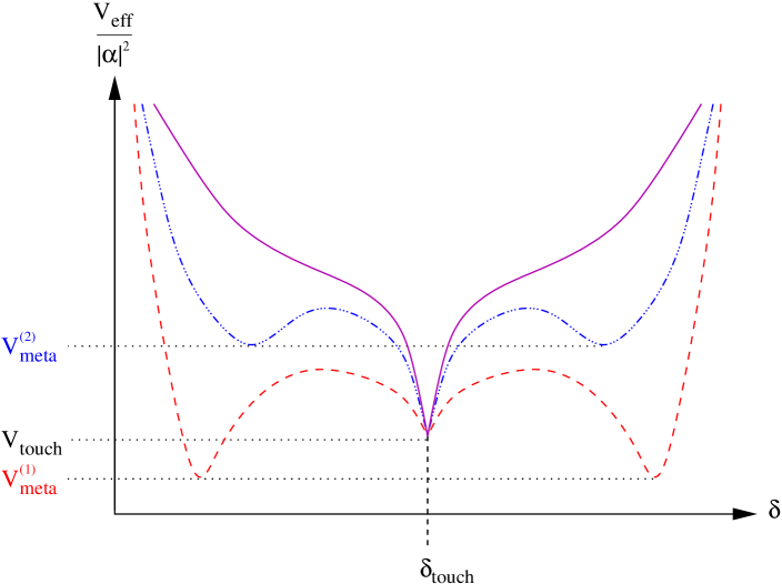
Figure 10: Depiction of $V_{\mathrm{eff}}/\left|\alpha\right|^{2}$ as a function of $\delta\equiv a_{1}^{+}-a_{1}^{-}=a_{2}^{+}-a_{2}^{-}>0$ with $N_{1}=-N_{2}\equiv N$.  The value of $V_{\mathrm{eff}}$ at the point where the cuts touch is independent of $N$.  When $N$ is small (dashed red), the system possesses a metastable minimum with energy density $V_{\mathrm{meta}}^{(1)}<V_{\mathrm{touch}}$.  For intermediate values of $N$ which still admit a metastable minimum (dot dashed blue), the energy density of the vacuum is $V_{\mathrm{meta}}^{(2)}>V_{\mathrm{touch}}$.  For large enough values of $N$ (solid purple), the system undergoes a phase transition and no metastable minimum exists.

7.1 Energy Near Cuts Touching

We now show that as the cuts touch along the locus $S_{1}=-S_{2}>0$, the effective potential approaches a constant value independent of $N$.  By virtue of equation (64), $V_{\mathrm{eff}}$ may be written as:

$$\frac{V_{\mathrm{eff}}}{\left|\alpha\right|^{2}}=\frac{1}{\tau_{++}+2\frac{M-\overline{M}}{2\pi i}}\left(4i-2i\left(\det\tau+\frac{M-\overline{M}}{2\pi i}\tau_{\mathrm{ell}}\right)\left|\frac{N}{\alpha}\right|^{2}\right)$$ (124)

where $\tau_{++}=\tau_{11}+\tau_{22}+2\tau_{12}$ is the “center of mass” coupling, $\tau_{\mathrm{ell}}=\tau_{11}+\tau_{22}-2\tau_{12}$ is the complex structure modulus of the elliptic curve, and as before, $M=\log\left(\Lambda_{0}^{2}/\Delta^{2}\right)$.  Note that as the cuts touch, $\tau_{\mathrm{ell}}$ tends to zero.  Because $\tau_{11}=\tau_{22}$, this implies $\tau_{12}$ tends to $\tau_{11}$ and thus $\det\tau$ tends to zero.   We therefore conclude that $V_{\mathrm{eff}}$ approaches the value:

$$V_{\mathrm{eff}}\rightarrow\frac{4i\left|\alpha\right|^{2}}{4\tau_{11}+2\frac{M-\overline{M}}{2\pi i}}\text{.}$$ (125)

Next, recall from appendix A that the behavior of $\tau_{11}$ is of the form $(B-M)/2\pi i$ where $B$ is a function of the moduli which is independent of $\alpha,N$ and $M$.  The value of $V_{\mathrm{touch}}$ is then:

$$V_{\mathrm{touch}}=\frac{2\pi\left|\alpha\right|^{2}}{B_{\mathrm{t}}+\log\left|\frac{\Lambda_{0}}{\Delta}\right|^{2}}$$ (126)

where $B_{\mathrm{t}}$ denotes the value of $B$ when the cuts touch.  This is manifestly independent of $N$.  Finally, we note that as $\Delta$ tends to zero, so too does $V_{\mathrm{touch}}$.

7.2 Flux Hysteresis

Close to the region in moduli space where the cuts touch, a gas of nearly tensionless D5-branes can cause the system to tunnel back out to a metastable configuration with lower flux.  This tunneling will cause the flux to undergo hysteresis.  In this subsection we determine the minimal size of this jump in the flux number.  Turning the discussion around, this also determines the range of values for which a metastable vacuum near the semi-classical expansion point can tunnel to the region where the cuts nearly touch.

Figure 11: Depiction of $V_{\mathrm{eff}}/\left|\alpha\right|^{2}$ as a function of $\delta\equiv a_{1}^{+}-a_{1}^{-}=a_{2}^{+}-a_{2}^{-}>0$ with $N_{1}=-N_{2}\equiv N$.  The figure shows flux configurations which possess a metastable minimum (dashed red) and those which do not (solid purple).  Close to the region in moduli space where the cycle $B_{1}-B_{2}$ collapses, the presence of nearly tensionless domain walls can cause the amount of flux to jump.  To reach a metastable minimum near the semi-classical expansion point, the moduli then either classically roll (a) or tunnel through moduli space (b).

We begin by characterizing the possible transition points for tunneling processes along the locus $S_{1}=-S_{2}>0$.  In addition to the metastable vacua near the semi-classical expansion point, there is another vacuum with identical energy where the branch cuts overlap almost completely.  To increase the scope of our discussion, we briefly consider more general configurations such that $S_{1}>0>S_{2}$.  With notation as in section 4, the endpoints of the branch cuts in the semi-classical regime satisfy $a_{1}^{+}>a_{1}^{-}>a_{2}^{+}>a_{2}^{-}$ with special coordinates defined by the integrals:

$$S_{1}=\frac{1}{2\pi i}\underset{a_{1}^{-}}{\overset{a_{1}^{+}}{\int}}ydx\text{ \ \ \ \ }S_{2}=-\frac{1}{2\pi i}\underset{a_{2}^{-}}{\overset{a_{2}^{+}}{\int}}ydx\text{.}$$ (127)

where the choice of signs is dictated by branch cut considerations.  In the region where the branch cuts overlap, we instead have $a_{1}^{+}>a_{2}^{+}>a_{1}^{-}>a_{2}^{-}$ with special coordinates defined by the integrals:

$$S_{1}^{\prime}=\frac{1}{2\pi i}\underset{a_{2}^{+}}{\overset{a_{1}^{+}}{\int}}ydx\ \ \ \ S_{2}^{\prime}=-\frac{1}{2\pi i}\underset{a_{2}^{-}}{\overset{a_{1}^{-}}{\int}}ydx.$$ (128)

It therefore follows from geometric considerations that there is a highly non-trivial duality in the low energy effective field theory between vacua with $S_{i}$ small and vacua with $S_{i}^{\prime}$ small.  In addition to these two physically indistinguishable configurations, there is the local singular minimum where the cuts touch.

The system can only tunnel from the region where the cuts touch to a metastable vacuum with small $S_{i}$ when:

$$V_{\mathrm{meta}}\leq V_{\mathrm{touch}}$$ (129)

where $V_{\mathrm{meta}}$ denotes the value of $V_{\mathrm{eff}}$ evaluated at such a metastable critical point and $V_{\mathrm{touch}}$ is given by equation (126).  Approximating $V_{\mathrm{meta}}$ by equation (82), the flux must therefore satisfy the bound:

$$g_{\mathrm{YM}}^{2}\left|N\right|\geq\frac{4\pi^{2}}{\log\left|\frac{\Lambda_{0}}{\Delta}\right|^{2}}\left(1-\sqrt{\frac{B_{\mathrm{t}}}{B_{\mathrm{t}}+\log\left|\frac{\Lambda_{0}}{\Delta}\right|^{2}}}\right)\text{.}$$ (130)

It now follows from equations (114) and (130) that in jumping from a flux configuration which does not admit a metastable vacuum near the semi-classical expansion point to one which does, the flux drops by an amount:

$$\delta\left|N\right|\geq\frac{4\pi^{2}}{g_{\mathrm{YM}}^{2}\log\left|\frac{\Lambda_{0}}{\Delta}\right|^{2}}\sqrt{\frac{B_{\mathrm{t}}}{B_{\mathrm{t}}+\log\left|\frac{\Lambda_{0}}{\Delta}\right|^{2}}}\text{.}$$ (131)

Turning the discussion around, the range of fluxes for which it is possible to tunnel from a metastable vacuum near the semi-classical expansion point to the region where the cuts touch is:

$$\frac{4\pi^{2}}{\log\left|\frac{\Lambda_{0}}{\Delta}\right|^{2}}\gtrsim g_{\mathrm{YM}}^{2}\left|N\right|\geq\frac{4\pi^{2}}{\log\left|\frac{\Lambda_{0}}{\Delta}\right|^{2}}\left(1-\sqrt{\frac{B_{\mathrm{t}}}{B_{\mathrm{t}}+\log\left|\frac{\Lambda_{0}}{\Delta}\right|^{2}}}\right)$$ (132)

where the crude upper bound follows from equation (114) and the requirement that a metastable minimum exists.  Note in particular that the admissible range of values of the ’t Hooft coupling which permit such a process is parametrically tied to the value for which metastability is lost.  Thus, nearly as soon as we increase the ’t Hooft coupling to a value where this quantum effect can contribute, it is overtaken by classical effects.

7.3 Dual Magnetic Description

Near the region in moduli space where the cuts touch, the fields $S_{1}$ and $S_{2}$ have become large and it is appropriate to change to a dual magnetic basis of fields.  From the perspective of the geometry, this corresponds to performing a change of basis which preserves the intersection pairing of the geometry.  Using this dual basis, we now show that the effective potential develops a cusp when the cuts touch.

The appropriate change of basis is dictated by the geometry of the Riemann surface.  Along the entire locus considered, $S_{1}+S_{2}$ has remained zero.  Further, the cycle $B_{1}-B_{2}$ is close to zero size.  This implies that the new $A$-cycles are $\widetilde{A}_{1}=B_{2}-B_{1}$ and $\widetilde{A}_{2}=A_{1}+A_{2}$.  Dual to these are new $B$-cycles $\widetilde{B}_{1}=A_{1}$ and $\widetilde{B}_{2}=B_{2}$.  Note that this new basis preserves the intersection pairing of the geometry.  The dual magnetic coordinates $\widetilde{S}_{i}$ and $\widetilde{\Pi}_{i}$ are therefore related to the original special coordinates by:

$$\widetilde{S}_{1} =\Pi_{2}-\Pi_{1}\text{ \ \ \ \ \ \ \ \ }\widetilde{S}_{2}=S_{1}+S_{2}$$ (133)

$$\widetilde{\Pi}_{1} =S_{1}\text{ \ \ \ \ \ \ \ \ \ \ \ \ \ \ \ }\widetilde{\Pi}_{2}=\Pi_{2}\text{. \ \ \ \ }$$ (134)

It follows from Picard-Lefschetz singularity theory that the only non-trivial monodromy arises from the transformation $\widetilde{S}_{1}\mapsto e^{2\pi i}\widetilde{S}_{1}$.  We therefore conclude that the leading order behavior of $\widetilde{\Pi}_{2}$ is regular and $\widetilde{\Pi}_{1}$ depends logarithmically on $\widetilde{S}_{1}$:

$$\widetilde{\Pi}_{1}=\frac{1}{2\pi i}\widetilde{S}_{1}\log\frac{\widetilde{S}_{1}}{g\Delta^{3}}+O(\widetilde{S}_{1}^{0})\text{.}$$ (135)

For a general flux configuration, the induced superpotential in the new coordinates is:

$$\mathcal{W}_{\mathrm{eff}}=\int H_{3}\wedge\Omega=\alpha\widetilde{S}_{2}+\left(N_{+}+N_{-}\right)\widetilde{S}_{1}+2N_{+}\widetilde{\Pi}_{2}$$ (136)

where $N_{\pm}\equiv\left(N_{2}\pm N_{1}\right)/2$.  Note that $\mathcal{W}_{\mathrm{eff}}$ is independent of $\widetilde{\Pi}_{1}$.  In particular, when $N_{1}=-N_{2}\equiv N$, the superpotential is independent of both of the $\widetilde{\Pi}_{i}$’s.  The entries of the new period matrix are:

$$\widetilde{\tau}_{ij}=\frac{\partial\widetilde{\Pi}_{j}}{\partial\widetilde{S}_{i}}.$$ (137)

Because $\widetilde{\Pi}_{2}$ is regular, we may approximate the Kähler metric as:

$$\operatorname{Im}\widetilde{\tau}_{ij}=-\frac{1}{4\pi}\left[\begin{array}[c]{cc}\log\left|\frac{\widetilde{S}_{1}}{g\Delta^{3}}\right|^{2}&c_{12}\\ c_{12}&c_{22}\end{array}\right]$$ (138)

where the $c_{ij}$ are non-zero constants.  In the new coordinates, the effective potential is:

$$V_{\mathrm{eff}}\left(\widetilde{S}_{1},\widetilde{S}_{2}\right)=\left[\begin{array}[c]{cc}-N&\alpha\end{array}\right]\frac{1}{\operatorname{Im}\widetilde{\tau}}\left[\begin{array}[c]{c}-N\\ \overline{\alpha}\end{array}\right]$$ (139)

in the obvious notation.  It therefore follows that $V_{\mathrm{eff}}$ attains a minimum at $\widetilde{S}_{1}=0$.

Replacing the $\widetilde{S}_{i}$ by fields $\widetilde{X}_{i}$ with canonically normalized kinetic terms, the derivative of $V_{\mathrm{eff}}$ with respect to $\widetilde{X}_{1}$ is:

$$\frac{\partial V_{\mathrm{eff}}}{\partial\widetilde{X}_{1}}\sim\frac{1}{\widetilde{S}_{1}}\frac{1}{f(\widetilde{S}_{1},\widetilde{S}_{2})}$$ (140)

where $f$ contains at most $\log\widetilde{S}_{1}$ type divergences.  We therefore conclude that the potential has a cusp at $\widetilde{S}_{1}=0$.

7.4 A Further Phase Transition

The singular behavior of the effective potential implies the presence of additional light states which have been integrated out.  As in the case of the conifold [41, 42], these light degrees of freedom correspond to a D3-brane wrapping the vanishing 3-cycle $B_{1}-B_{2}$.  In $\mathcal{N}=2$ language, this corresponds to a hypermultiplet which is charged under the gauge boson of the $U(1)$ vector multiplet with scalar component $\widetilde{S}_{1}$.  The superpotential is now:

$$\mathcal{W}_{\mathrm{eff}}=\alpha\widetilde{S}_{2}+\left(N_{+}+N_{-}\right)\widetilde{S}_{1}+2N_{+}\widetilde{\Pi}_{2}+h\widetilde{S}_{1}Q_{L}Q_{R}$$ (141)

where $h$ is a Yukawa coupling and $Q_{L}$ and $Q_{R}$ denote the $\mathcal{N}=1$ chiral multiplets of the hypermultiplet.  At a critical point of $V_{\mathrm{eff}}$, the $Q$’s condense with expectation value:

$$\left\langle Q_{L}Q_{R}\right\rangle=\frac{N}{h}\text{.}$$ (142)

This condensate signals the presence of a new holomorphic 2-cycle $\Sigma=\partial A_{1}$ in the geometry with size $\left|N/h\right|$.  Perhaps surprisingly, the resulting manifold is non-Kähler!

To see this, let us suppose to the contrary that the new geometry is a Calabi-Yau threefold.  In this case, the absence of any other normalizable $(1,1)$ forms implies that the $(1,1)$ form $k_{\Sigma}$ which measures the volume of $\Sigma$ determines the local metric of the new geometry.  It now follows from Stokes’ theorem that:

$$\underset{A_{1}}{\int}dk_{\Sigma}=\underset{\Sigma}{\int}k_{\Sigma}\neq 0\text{.}$$ (143)

This implies that $k_{\Sigma}$ is not closed.  We therefore conclude that the resulting manifold is not a Calabi-Yau threefold, but instead belongs to the category of generalized Calabi-Yau threefolds [43].  While it is doubtful that the resulting physical configuration is supersymmetric or even metastable, a proper analysis is beyond the scope of this paper and we defer a full study of this question to future work.

8 Conclusions

In this paper we have studied the phase structure of a strongly coupled supersymmetry breaking configuration of D5-branes and anti-D5-branes wrapped over homologous rigid $S^{2}$’s of a non-compact Calabi-Yau threefold using the large $N$ dual description of this system.  In much of this paper we focused on the closed string dual geometry with two branch cuts.  Even in this simple case, higher order corrections to the potential for the glueball fields generate an elaborate phase structure which can already be seen at the two loop level.  Near the semi-classical expansion point, this two loop effect lifts the degeneracy in energy density between the many confining vacua of the theory.  When the scale of confinement is not exponentially suppressed, this generates a large number of additional metastable vacua.  For sufficiently large values of the ’t Hooft coupling this same effect also lifts the metastable vacua present at weak coupling.  After this phase transition, the branch cuts expand in size until they are close to touching.  Although the presence of nearly tensionless domain walls close to this region of moduli space will most likely cause the system to relax to a metastable vacuum of lower flux, the presence of new massless states when the cuts touch may also allow the geometry to transition to a non-Kähler manifold.  We now discuss some implications of this work.

As the separation $\Delta$ between the branes decreases, the glueball potential develops an instability.  Although it is tempting to identify this instability with the open string theory tachyon, there is a potentially serious problem with this interpretation.  Indeed, it follows from equation (114) that the effective potential develops an instability when:

$$\frac{1}{g_{\mathrm{YM}}^{2}\left|N\right|}\sim\log\left|\frac{\Lambda_{0}}{\Delta}\right|^{2}\text{.}$$ (144)

On the other hand, the tachyonic mode of the brane/anti-brane system is independent of $N$ because this constant factors out of all relevant open string amplitudes.  We therefore conclude that an identification of the two instabilities is not naively correct.

We have also seen a preliminary indication that the number of critical points of $V_{\mathrm{eff}}$ crucially depends on the amount of flux in the closed string holographic dual.  As this amount of flux changes, a local maximum and minimum may merge.  Such a change in the number of metastable minima cannot be detected by a Morse-theoretic index.  This may have implications for recent attempts to count the number of supersymmetry breaking vacua in flux compactifications.  Indeed, many of the techniques developed thus far rely on similar indices to count the number of admissible vacua [44].  It would therefore be interesting to determine whether such methods properly account for the metastable vacua studied in this paper.

Although a more detailed analysis of the phase structure near the region of moduli space where the branch cuts touch will most likely be difficult, we have seen that when $N_{1}\sim-N_{2}$, the geometry may undergo a further phase transition to a non-Kähler manifold.  Even so, the decay of the vacuum due to flux line annihilation may obstruct this intriguing possibility from contributing to the phase structure of the theory.  It is likely that a proper description of the effective theory near this region in moduli space will require a more generalized effective potential which treats both the moduli and the fluxes as dynamical variables.  Even if the geometry can transition to a non-Kähler manifold, the resulting configuration is unlikely to be stable.  It would be interesting to determine the endpoint of this further phase transition.

In much of this paper we restricted our analysis to the two cut geometry.  While this should provide an adequate characterization of “two body” interactions, it is possible that the interaction of three or more cuts could lead to further novel phases.  Although we still expect the phases of the glueball fields to align in an energetically preferred configuration, the relative orientation between the cuts will depend on the location of the $a_{i}$.  Indeed, treating the branch cuts as small dipole moments, an energetically preferred configuration may be frustrated for a large lattice of cuts, much as in the two dimensional Ising model on a triangular lattice.  It is well-known in the setting of condensed matter systems that magnetic frustration can produce novel phases such as spin liquids and glasses.  It is therefore likely that a similarly rich class of phenomena are present in metastable multi-cut geometries.

Appendix A: Two Cut Semi-Classical $\tau_{ij}$ and $\mathcal{F}_{ijk}$

In this appendix we collect explicit expressions for $\tau_{ij}$ and $\mathcal{F}_{ijk}=\partial_{i}\tau_{jk}$ for the two cut geometry defined by equation (5).  Setting $\Delta\equiv a_{1}-a_{2}$, $t_{1}\equiv S_{1}/g\Delta^{3}$ and $t_{2}\equiv-S_{2}/g\Delta^{3}$, we have [18]:

$$2\pi i\tau_{11} =\log t_{1}-\log\frac{\Lambda_{0}^{2}}{\Delta^{2}}+\left(4t_{1}+10t_{2}\right)+\left(32t_{1}^{2}+182t_{1}t_{2}+118t_{2}^{2}\right)+O(t^{3})$$ (145)

$$2\pi i\tau_{12} =-\log\frac{\Lambda_{0}^{2}}{\Delta^{2}}+\left(-10t_{1}-10t_{2}\right)+\left(-91t_{1}^{2}-236t_{1}t_{2}-91t_{2}^{2}\right)+O(t^{3})$$ (146)

$$2\pi i\tau_{22} =\log t_{2}-\log\frac{\Lambda_{0}^{2}}{\Delta^{2}}+\left(4t_{2}+10t_{1}\right)+\left(32t_{2}^{2}+182t_{1}t_{2}+118t_{1}^{2}\right)+O(t^{3}),$$ (147)

and:

$$2\pi ig\Delta^{3}\mathcal{F}_{111} =\frac{1}{t_{1}}+4+\left(64t_{1}+182t_{2}\right)+O(t^{2})$$ (148)

$$2\pi ig\Delta^{3}\mathcal{F}_{112} =-10+\left(-182t_{1}-236t_{2}\right)+O(t^{2})$$ (149)

$$2\pi ig\Delta^{3}\mathcal{F}_{122} =10+236t_{1}+182t_{2}+O(t^{2})$$ (150)

$$2\pi ig\Delta^{3}\mathcal{F}_{222} =-\frac{1}{t_{2}}-4-64t_{2}-182t_{1}+O(t^{2}).$$ (151)

Appendix B: Mass Spectrum for $\left|N_{1}\right|\gg\left|N_{2}\right|$

In this appendix we compute the bosonic and fermionic masses for flux configurations with $\left|N_{1}\right|\gg\left|N_{2}\right|$, $\theta_{\mathrm{YM}}=0$ and $S_{1}>0>S_{2}$.  With the kinetic terms of the Lagrangian density canonically normalized, the $4\times 4$ bosonic mass squared matrix $m_{\mathrm{Bosonic}}^{2}$ takes the block diagonal form:

$$m_{\mathrm{Bosonic}}^{2}=A^{(R)}\oplus A^{(I)}$$ (152)

where the $A^{(R,I)}$ are $2\times 2$ matrices of the form:

$$A^{(R,I)}=\left(\begin{array}[c]{cc}\frac{\left(\partial_{1}^{(R,I)}+\partial_{2}^{(R,I)}\right)^{2}V_{\mathrm{eff}}}{1+v}&-\frac{\left(\partial_{1}^{(R,I)}-\partial_{2}^{(R,I)}\right)\left(\partial_{1}^{(R,I)}+\partial_{2}^{(R,I)}\right)V_{\mathrm{eff}}}{\sqrt{1-v^{2}}}\\ -\frac{\left(\partial_{1}^{(R,I)}-\partial_{2}^{(R,I)}\right)\left(\partial_{1}^{(R,I)}+\partial_{2}^{(R,I)}\right)V_{\mathrm{eff}}}{\sqrt{1-v^{2}}}&\frac{\left(\partial_{1}^{(R,I)}-\partial_{2}^{(R,I)}\right)^{2}V_{\mathrm{eff}}}{1-v}\end{array}\right)$$ (153)

and $A^{(R)}$ ($A^{(I)}$) corresponds to the mass matrix for the real (imaginary) components of the $S_{i}$’s.  In the above we have defined:

$$\partial_{j}^{(R)}=\frac{1}{\sqrt{\operatorname{Im}\tau_{jj}}}\frac{\partial}{\partial\operatorname{Re}S_{j}},\text{ }\partial_{j}^{(I)}=\frac{1}{\sqrt{\operatorname{Im}\tau_{jj}}}\frac{\partial}{\partial\operatorname{Im}S_{j}},\text{ }v=\frac{\operatorname{Im}{{\tau}_{12}}^{2}}{\mathrm{\operatorname{Im}}{\tau}_{11}\operatorname{Im}{\tau}_{22}},$$ (154)

and for future use we also introduce:

$$a=\frac{|N_{1}|}{2\pi t_{1}\operatorname{Im}{\tau}_{11}}\text{, }b=\frac{|N_{2}|}{2\pi t_{2}\operatorname{Im}{\tau}_{22}}.$$ (155)

In the above expressions the components of $\tau_{ij}$ correspond to their value at the critical point of $V_{\mathrm{eff}}$ and should therefore be treated as constants.  When $\left|N_{1}\right|>>|N_{2}|$, the masses squared and eigenmodes of the block $A^{(R)}$ are:

$$m_{\operatorname{Re}S_{1}}^{2} =\frac{b^{2}}{(1-v)^{2}} \left(\sqrt{\frac{1-\sqrt{v}}{1+\sqrt{v}}},1\right)_{R} \oplus\left(0,0\right)_{I}$$ (156)

$$m_{\operatorname{Re}S_{2}}^{2} =a^{2}-2a\left(10|N_{2}|-\frac{2|N_{1}|+5|N_{2}|}{\operatorname{Im}{\tau}_{11}\pi}\right) \left(-\sqrt{\frac{1+\sqrt{v}}{1-\sqrt{v}}},1\right)_{R} \oplus\left(0,0\right)_{I}$$ (157)

and the masses squared and eigenmodes of the block $A^{(I)}$ are similarly:

$$m_{\operatorname{Im}S_{1}}^{2} =\frac{b^{2}}{(1-v)^{2}} \left(\sqrt{\frac{1-\sqrt{v}}{1+\sqrt{v}}},1\right)_{I}\oplus \left(0,0\right)_{R}$$ (158)

$$m_{\operatorname{Im}S_{2}}^{2} =a^{2}+2a\left(10|N_{2}|+\frac{2|N_{1}|+5|N_{2}|}{\operatorname{Im}{\tau}_{11}\pi}\right) \left(-\sqrt{\frac{1+\sqrt{v}}{1-\sqrt{v}}},1\right)_{I}\oplus \left(0,0\right)_{R}\text{.}$$ (159)

Grouping the fermions according to the supermultiplet structure inherited from the $\mathcal{N}=1$ supersymmetry of the branes, the non-zero fermion masses are:

$$m_{\psi_{S}} =\frac{1}{1-v}\left(a+\frac{2|N_{1}|+5|N_{2}|+10|N_{1}|\frac{\operatorname{Im}{\tau}_{12}}{\operatorname{Im}{\tau}_{22}}}{\operatorname{Im}{\tau}_{11}\pi}\right)$$ (160)

$$m_{\psi_{A}} =\frac{1}{1-v}\left(b+\frac{2|N_{2}|+5|N_{1}|+10|N_{1}|\frac{\operatorname{Im}{\tau}_{12}}{\operatorname{Im}{\tau}_{11}}}{\operatorname{Im}{\tau}_{22}\pi}\right)$$ (161)

with similar notation to that given above equation (120).  By inspection of the above formulae, we see that the two loop correction increases the difference between the bosonic and fermionic masses already present at leading order.

Keeping $g_{\mathrm{YM}}^{2}\left|N_{2}\right|$ fixed, we now determine the mode which develops an instability as the ’t Hooft coupling $g_{\mathrm{YM}}^{2}\left|N_{1}\right|$ approaches the critical value where the original metastable vacua disappear.  The determinant of each block of the mass matrix is:

$$\det A^{(R)} =\frac{4096\pi^{8}\log t_{1}\log t_{2}}{g_{YM}^{8}t_{1}^{2}t_{2}^{2}\left(\log t_{1}\log t_{2}-\log\frac{|{\Lambda}_{0}|^{2}}{{|\Delta|}^{2}}\left(\log t_{1}+\log t_{2}\right)\right)^{6}}$$ (162)

$$\times\left(\begin{array}[c]{l}\log t_{1}\log t_{2}-20t_{1}\left(\log t_{1}\right)^{2}\left(\log\frac{|{\Lambda}_{0}|^{2}}{{|\Delta|}^{2}}-\log t_{1}\right)\\ -20t_{2}\left(\log t_{2}\right)^{2}\left(\log\frac{|{\Lambda}_{0}|^{2}}{{|\Delta|}^{2}}-\log t_{2}\right)+\cdots\end{array}\right)$$ (165)

$$\det A^{(I)} =\frac{4096\pi^{8}\log t_{1}\log t_{2}}{g_{YM}^{8}t_{1}^{2}t_{2}^{2}\left(\log t_{1}\log t_{2}-\log\frac{|{\Lambda}_{0}|^{2}}{{|\Delta|}^{2}}\left(\log t_{1}+\log t_{2}\right)\right)^{6}}$$ (166)

$$\times\left(\begin{array}[c]{l}\log t_{1}\log t_{2}+20t_{1}\left(\log t_{1}\right)^{2}\left(\log\frac{|{\Lambda}_{0}|^{2}}{{|\Delta|}^{2}}-\log t_{1}\right)\\ +20t_{2}\left(\log t_{2}\right)^{2}\left(\log\frac{|{\Lambda}_{0}|^{2}}{{|\Delta|}^{2}}-\log t_{2}\right)+\cdots\end{array}\right).$$ (169)

It follows from the last line of each expression that only $m_{\operatorname{Re}S_{1}}^{2}$ or $m_{\operatorname{Re}S_{2}}^{2}$ can vanish.  Furthermore, because $m_{\operatorname{Re}S_{1}}^{2}>>m_{\operatorname{Re}S_{2}}^{2}$, the mode of instability will cause the smaller cut to expand towards the larger cut.  For $\left|N_{1}\right|\gg\left|N_{2}\right|~{}$this occurs at a value of $t_{1}$ given by:

$$1\sim 20\left(-\log t_{1}+\log\left|\frac{{\Lambda}_{0}}{{\Delta}}\right|^{2}\right)t_{1}.$$ (170)

Note that this is similar in form to the critical value of the moduli found in equation (112) for the case $N_{1}=-N_{2}$.

References

- [1] C. Vafa, “Superstrings and Topological Strings at Large N,” J. Math. Phys. 42 (2001) 2798–2817, hep-th/0008142.
- [2] S. Kachru, J. Pearson, and H. Verlinde, “Brane/Flux Annihilation and the String Dual of a Non-Supersymmetric Field Theory,” JHEP 0206 (2002) 021, hep-th/0112197.
- [3] S. Kachru, R. Kallosh, A. Linde, and S. P. Trivedi, “de Sitter Vacua in String Theory,” Phys. Rev. D 68 (2003) 046005, hep-th/0301240.
- [4] S. Kachru and J. McGreevy, “Supersymmetric Three-cycles and (Super)symmetry Breaking,” Phys. Rev. D 61 (2000) 026001, hep-th/9908135.
- [5] R. Argurio, M. Bertolini, S. Franco, and S. Kachru, “Gauge/gravity duality and meta-stable dynamical supersymmetry breaking,” JHEP 0701 (2007) 083, hep-th/0610212.
- [6] M. Aganagic, C. Beem, J. Seo, and C. Vafa, “Geometrically Induced Metastability and Holography,” hep-th/0610249.
- [7] H. Verlinde, “On Metastable Branes and a New Type of Magnetic Monopole,” hep-th/0611069.
- [8] K. Intriligator, N. Seiberg, and D. Shih, “Dynamical SUSY Breaking in Meta-Stable Vacua,” JHEP 0604 (2006) 021, hep-th/0602239.
- [9] H. Ooguri and Y. Ookouchi, “Meta-Stable Supersymmetry Breaking Vacua on Intersecting Branes,” Phys. Lett. B 641 (2006) 323–328, hep-th/0607183.
- [10] S. Franco, I. Garcia-Etxebarria, and A. M. Uranga, “Non-supersymmetric Meta-stable Vacua from Brane Configurations,” JHEP 0701 (2007) 085, hep-th/0607218.
- [11] I. Bena, E. Gorbatov, S. Hellerman, N. Seiberg, and D. Shih, “A Note on (Meta)stable Brane Configurations in MQCD,” JHEP 0611 (2006) 088, hep-th/0608157.
- [12] R. Tatar and B. Wetenhall, “Metastable Vacua, Geometrical Engineering and MQCD Transitions,” JHEP 0702 (2007) 020, hep-th/0611303.
- [13] J. M. Maldacena, “The Large N Limit of Superconformal field theories and supergravity,” Adv. Theor. Math. Phys. 2 (1998) 231–252, hep-th/9711200.
- [14] S. S. Gubser, I. R. Klebanov, and A. M. Polyakov, “Gauge Theory Correlators from Non-Critical String Theory,” Phys. Lett. B428 (1998) 105–114, hep-th/9802109.
- [15] E. Witten, “Anti De Sitter Space and Holography,” Adv. Theor. Math. Phys. 2 (1998) 253–291, hep-th/9802150.
- [16] I. R. Klebanov and M. J. Strassler, “Supergravity and a Confining Gauge Theory: Duality Cascades and SB-Resolution of Naked Singularities,” JHEP 0008 (2000) 052, hep-th/0007191.
- [17] J. M. Maldacena and C. Nunez, “Towards the large limit of pure Super Yang Mills,” Phys. Rev. Lett. 86 (2001) 588–591, hep-th/0008001.
- [18] F. Cachazo, K. Intriligator, and C. Vafa, “A Large N Duality via a Geometric Transition,” Nucl. Phys. B 603 (2001) 3–41, hep-th/0103067.
- [19] R. Dijkgraaf and C. Vafa, “Matrix Models, Topological Strings, and Supersymmetric Gauge Theories,” Nucl. Phys. B 644 (2002) 3–20, hep-th/0206255.
- [20] R. Dijkgraaf and C. Vafa, “On Geometry and Matrix Models,” Nucl. Phys. B 644 (2002) 21–39, hep-th/0207106.
- [21] R. Dijkgraaf and C. Vafa, “A Perturbative Window into Non-Perturbative Physics,” hep-th/0208048.
- [22] E. Witten, “Large N Chiral Dynamics,” Ann. Phys. 128 (1980) 363–375.
- [23] E. Witten, “Theta Dependence in The Large Limit Of Four-Dimensional Gauge Theories,” Phys. Rev. Lett. 81 (1998) 2862–2865, hep-th/9807109.
- [24] M. A. Shifman, “Domain walls and the decay rate of the excited vacua in large Yang-Mills theory,” Phys. Rev. D 59 (1999) 021501, hep-th/9809184.
- [25] S. Gukov, C. Vafa, and E. Witten, “CFT’s From Calabi-Yau Four-folds,” Nucl. Phys. B 584 (2000) 69–108 [Erratum–ibid. B 608 (2001) 477–478], hep-th/9906070.
- [26] H. Ooguri and C. Vafa, “Worldsheet Derivation of a Large N Duality,” Nucl. Phys. B 641 (2002) 3–34, hep-th/0205297.
- [27] R. Dijkgraaf, S. Gukov, V. A. Kazakov, and C. Vafa, “Perturbative Analysis of Gauged Matrix Models,” Phys. Rev. D 68 (2003) 045007, hep-th/0210238.
- [28] S. Ferrara, R. Kallosh, and A. Strominger, “ Extremal Black Holes,” Phys. Rev. D 52 (1995) 5412–5416, hep-th/9508072.
- [29] A. Strominger, “Macroscopic Entropy of Extremal Black Holes,” Phys. Lett. B 383 (1996) 39–43, hep-th/9602111.
- [30] S. Ferrara and R. Kallosh, “Supersymmetry and Attractors,” Phys. Rev. D 54 (1996) 1514–1524, hep-th/9602136.
- [31] S. Ferrara and R. Kallosh, “Universality of Supersymmetric Attractors,” Phys. Rev. D 54 (1996) 1525–1534, hep-th/9603090.
- [32] S. R. Coleman, “Fate Of the False Vacuum: Semiclassical Theory,” Phys. Rev. D 15 (1977) 2929–2936 [Erratum–ibid. D. 16, 1248 (1977)].
- [33] E. Witten, “Current Algebra Theorems For The ‘Goldstone Boson’,” Nucl. Phys. B 156 (1979) 269–283.
- [34] M. A. Shifman, “Non-Perturbative Dynamics in Supersymmetric Gauge Theories,” Prog. Part. Nucl. Phys. 39 (1997) 1–116, hep-th/9704114.
- [35] N. Evans, S. D. H. Hsu, and M. Schwetz, “Controlled Soft Breaking of SQCD,” Phys. Lett. B 404 (1997) 77–82, hep-th/9703197.
- [36] I. Halperin and A. Zhitnitsky, “On Topological Susceptibility, Vacuum Energy and Theta,” Mod. Phys. Lett. A 13 (1998) 1955–1967, hep-ph/9707286.
- [37] I. Halperin and A. Zhitnitsky, “Can Dependence for Gluodynamics be Compatible with Periodicity in ?,” Phys. Rev. D 58 (1998) 054016, hep-ph/9711398.
- [38] I. Halperin and A. Zhitnitsky, ““Integrating in” and Effective Lagrangian for Non-Supersymmetric Yang-Mills Theory,” Nucl. Phys. B 539 (1999) 166–186, hep-th/9802095.
- [39] I. Halperin and A. Zhitnitsky, “Anomalous Effective Lagrangian and Dependence in QCD at Finite ,” Phys. Rev. Lett. 81 (1998) 4071–4074, hep-ph/9803301.
- [40] A. Zhitnitsky, “Topological defects and dependence in QCD,” Nucl. Phys. Proc. Suppl. 73 (1999) 647–649.
- [41] A. Strominger, “Massless Black Holes and Conifolds in String Theory,” Nucl. Phys. B 451 (1995) 96–108, hep-th/9504090.
- [42] B. Greene, D. Morrison, and A. Strominger, “Black Hole Condensation and the Unification of String Vacua,” Nucl. Phys. B 451 (1995) 109–120, hep-th/9504145.
- [43] N. Hitchin, “Generalized Calabi-Yau Manifolds,” Q. J. Math. 54 (2003) 281–308, math.DG/0209099.
- [44] S. Ashok and M. R. Douglas, “Counting Flux Vacua,” JHEP 0401 (2004) 060, hep-th/0307049.