We present new solutions of noncommutative gauge theories in which coincident unstable vortices expand into unstable circular shells. As the theories are noncommutative, the naive definition of the locations of the vortices and shells is gauge-dependent, and so we define and calculate the profiles of these solutions using the gauge-invariant noncommutative Wilson lines introduced by Gross and Nekrasov. We find that charge 2 vortex solutions are characterized by two positions and a single nonnegative real number, which we demonstrate is the radius of the shell. We find that the radius is identically zero in all 2-dimensional solutions. If one considers solutions that depend on an additional commutative direction, then there are time-dependent solutions in which the radius oscillates, resembling a braneworld description of a cyclic universe. There are also smooth BIon-like space-dependent solutions in which the shell expands to infinity, describing a vortex ending on a domain wall.

1 Introduction

Noncommutative gauge theories with or without adjoint scalars and/or fundamental fermions are known to admit unstable vortex solutions. The shapes and positions of these noncommutative vortices are difficult to describe or even define, as the positions of the gauge field, scalars and fermions are gauge dependent. In Ref. [1] the authors introduced two kinds of gauge-invariant operators, a fermion bilinear and also a trace of the gauge field in momentum space which allow one to define and measure the positions of these configurations in a gauge-invariant way. They arrived at the interesting conclusion that the positions of a set of vortices are the eigenvalues of its Weyl-transformed Wilson lines.

In this note we demonstrate that, if a vortex charge is greater than one, then there are new gauge-invariant quantities which are distinguished by both gauge-invariant operators. We find that the equations of motion demand that these quantities vanish in the 2-dimensional theories described in Ref. [1], but not in higher-dimensional analogues. We find the positions of these new solutions by calculating the Fourier transform of the trace of the momentum space wavefunction, which following [1] is defined to be a kind of noncommutative Wilson loop.

In the case of coincident charge 2 vortices, we find solutions in which a codimension 2 vortex expands into a thin circular domain wall reminiscent of the commutative solitons in Refs. [2, 3, 4]. Unlike non-BPS semilocal vortices [5, 6] in commutative gauge theories, the domain wall appears to have a sharp outer boundary, although a change in normalization of the Wilson loops would smoothen this boundary. There is precisely one new nonnegative real gauge-invariant quantity in the charge 2 case, which we show corresponds to the radius of this shell. The radius is proportional to the commutator of the gauge fields in the transverse directions, analogously to the construction of higher dimensional D-branes from lower dimensional D-branes with noncommuting position matrices, in keeping with the identification of the gauge field eigenvalues and the positions in Refs. [7, 1]. In solutions with dependence on an additional commutative spatial dimension, this circle grows to infinity, reaching infinity at a finite position, and so describes a vortex ending on a domain wall. If instead one considers time-dependent solutions with 2 noncommutative spatial dimensions, then the radius oscillates periodically in the commutative time direction. If one includes fundamental fermions, then when the radius vanishes there are two fermion zero modes, of which one is lifted by a nonvanishing radius.

2 Vortices in the 2d theory

2.1 The gauge theory

Consider bosonic string theory on the space $M^{24}\times\mathbb{R}^{2}$ where $M^{24}$ is an arbitrary 24-manifold. Wrap a single spacefilling D25-brane on the entirety of spacetime, and consider a $B$-field that is constant and has both legs along $\mathbb{R}^{2}$. The spectrum of open strings ending on this D25-brane includes massless vectors which are gauge bosons for a $U(1)$ gauge symmetry.

The $U(1)$ gauge bundle has a curvature $F$. However the open strings couple to $F$ in the combination $B+F$, which means that covariant derivatives acting on charged fields have contributions not only from the vector potential $iA$ of $F$, but also for that of $B$. We will refer to the total vector potential as $C$. In particular, even if $F=0$ then the wavefunction of a particle traveling around a loop $\gamma$ gains a phase equal to the loop-integral of $C$ which is equal by Stoke’s theorem to the integral of $B$ on the interior $D$ of the loop

$$\int_{\gamma}C=\int_{D}dC=\int_{D}B+F=\int_{D}B$$ (2.1)

where $\partial D=\gamma$. Equivalently, if $x$ and $y$ are a set of coordinates on $\mathbb{R}^{2}$, then if a charged particle moves first in the $x$ direction and then in the $y$ direction, its phase will not be the same as if it moved first in the $y$ direction and then in the $x$ direction. For this reason this theory is called a noncommutative $U(1)$ gauge theory. In particular, the fact that translations in $x$ and $y$ do not commute means that the $x$ and $y$ translation generators, the momenta, do not commute. In turn this implies that the operators $x$ and $y$ themselves do not commute.

Although the $\mathbb{R}^{2}$ direction is noncompact, if we are interested in solutions which are normalizable in the $\mathbb{R}^{2}$ direction we may dimensionally reduce the theory to a 24-dimensional theory on $M^{24}$. Consider two of the 26-dimensional fields, the adjoint scalar $\phi$ and the $U(1)$ gauge field $A$. At each point in the 24-dimensional space $M^{24}$, $\phi$ and $A$ are functions of $x$ and $y$. As they are normalizable, these functions may be expanded in terms of Laguerre polynomials, which are a countably infinite basis of functions. The coefficients of these polynomials may be arranged in two infinite-dimensional matrices, which by an abuse of notation we will also refer to as $\phi$ and $A$ such that the noncommutativity of the $x$ and $y$ dependence is captured by the noncommutativity of matrix multiplication. We can even write the full connection $C$ as a matrix. These infinite-dimensional matrices are known as the Weyl transforms of the $\mathbb{R}^{2}$-dependent fields.

$iA$ and $C$ are both vectors, and so are described by 26 Hermitian matrices, one for each component. We will define

$$A=A_{x}+iA_{y},\hskip 19.91684pt\overline{A}=A_{x}-iA_{y},\hskip 19.91684ptC=C_{x}+iC_{y},\hskip 19.91684pt\ \overline{C}=C_{x}-iC_{y}.$$ (2.2)

Rescaling the $\mathbb{R}^{2}$ coordinates so that the commutator of $x$ and $y$ is equal to $i$, corresponding to $\theta=1$ in the usual parametrization, one finds that $x+iy$ and $x-iy$ represent the generators $a$ and $a^{\dagger}$ of the Heisenberg algebra. Therefore we may choose a convention in which

$$C=a{}^{\dagger}-iA,\hskip 19.91684pt\overline{C}=a+i\overline{A}.$$ (2.3)

Recall that $iA_{x}$, $iA_{y}$, $C_{x}$ and $C_{y}$ are Hermitian, and so $iA$, $i\overline{A}$, $C$ and $\overline{C}$ will generally not be Hermitian and need not even be diagonalizable.

The Weyl transformed $A$ is the connection for a 24-dimensional $U({\cal{H}})$ gauge theory. If all fields, like $A$ and $\phi$, transform in the adjoint of the gauge group then the center $U(1)\subset U({\cal{H}})$ acts trivially. This means that the fields form representations of the smaller gauge group

$$PU({\cal{H}})=\frac{U({\cal{H}})}{U(1)}$$ (2.4)

and only the $PU({\cal{H}})$ gauge bundle needs to be well-defined. The effective gauge group $PU({\cal{H}})$ is an Eilenberg-MacLane space with nontrivial homotopy group

$$\pi_{2}(PU({\cal{H}}))=\mathbb{Z}$$ (2.5)

and so nontrivial gauge bundles are characterized entirely by an integral 3-class $H$, which will be identified with the NS 3-form.

The gauge groups $U({\cal{H}})$ and $PU({\cal{H}})$ only appear after the dimensional reduction from 26 to 24 dimensions, and so it appears that the gauge bundle is fibered over only a 24-dimensional subspace of the 26-dimensional spacetime, although in principal its characteristic class $H$ is defined on the entire bulk. This is because we chose to start with a single D25-brane. The Sen conjecture [10] has taught us that the open strings on a single D25-brane do not capture all of the physics, one needs an infinite stack. In the AdS/CFT correspondence [11, 12, 13] this corresponds to the fact that the open strings that end on an infinite stack of D-branes know everything about the closed string sector. Therefore to capture all of the information about the string theory, one would have needed an infinite stack of D25-branes, which would have led to the desired $PU({\cal{H}})$ bundle over the bulk. This may appear to be in contradiction with the possibility that the $H$ flux is nontrivial around some cycle, which would disallow a spacefilling brane, indeed the Sen picture breaks down in that case and it is harder to find the closed strings in the open string physics.

We will first consider configurations which are constant on $M^{24}$, yielding a 2-dimensional Euclidean gauge theory which is dimensionally reduced to a 0-dimensional matrix model via the Weyl transform. Let

$$w=\frac{1}{\sqrt{2}}(x+iy),\hskip 19.91684pt\overline{w}=\frac{1}{\sqrt{2}}(x-iy)$$ (2.6)

be complex coordinates on the $\mathbb{R}^{2}$. We will use the symbols $\partial$ and $\overline{\partial}$ for derivatives which are covariant with respect to the connection of the $B$ field but not the gauge field in the directions $w$ and $\overline{w}$ respectively. We have seen that these represent the usual raising and lower operators in the Heisenberg algebra.

Using these derivatives and the $U(1)$ gauge potential $A$, which is dimensionally reduced to a $U({\cal{H}})$ gauge potential in the matrix model, we may define a $U({\cal{H}})$ field strength

$$F_{w\overline{w}}=\partial\overline{A}-\overline{\partial}A-i[A,\overline{A}]=-i[C,\overline{C}]-i.$$ (2.7)

In terms of this field strength, and the adjoint scalar $\phi$ we may write the action for our matrix model following, for example, Ref. [8]

$$S=2\pi\hbox{\rm Tr}_{{\cal{H}}}(-\frac{1}{4}F_{ij}F^{ij}-[C,\phi][\overline{C},\phi]-V(\phi))$$ (2.8)

where $V(\phi)$ is a potential function with a local maximum at $\phi=0$ and a local minimum at $\phi=1$.

We may now obtain equations of motion by varying the action with respect to $\phi$, $C$ and $\overline{C}$. In the square of $F$, the $[C,\overline{C}]$ and $1$ terms are both topological and so do not contribute to the equations of motion, thus we need only consider the $[\overline{C},C]^{2}$ term.

Varying $\phi$ one obtains the equation of motion

$$0=[\overline{C},[C,\phi]]-V{}^{\prime}(\phi).$$ (2.9)

Varying $C$ one finds

$$[\overline{C},[\overline{C},C]-[\phi,[\overline{C},\phi]]=0$$ (2.10)

and varying $\overline{C}$ we find its transpose

$$[C,[C,\overline{C}]-[\phi,[C,\phi]]=0.$$ (2.11)

Now we are ready to choose an ansatz and solve these equations. The adjoint scalar will not play a crucial role in the solutions that we will present, they will all have analogues in a truncated theory in which one omits the $\phi$ field entirely.

2.2 Two-dimensional solutions and symmetries

We will be interested in an solutions describing $N$ point-like branes. This corresponds to the ansatz

$$\phi=\phi_{*}(1-P_{N})$$ (2.12)

where $1$ is the identity matrix, $P_{N}$ is the projector onto an $N$-dimensional subspace $\mathbb{C}^{N}\subset{\cal{H}}$ and $\phi_{*}$ is the stable minimum of $V(\phi)$. In Ref. [14] the authors demonstrated that in this ansatz the potential term vanishes in the $\phi$ equation of motion (2.9).

The projector decomposes the Hilbert space ${\cal{H}}$ into its eigenspaces, a $\mathbb{C}^{N}$ which it annihilates and the remaining ${\cal{H}}$ on which it has eigenvalue one. We can use this decomposition to decompose $C$ and $\overline{C}$ in terms of an $N\times N$, an $N\times\infty$, an $\infty\times N$ and an $\infty\times\infty$ submatrix

$$C=\left(\begin{array}[]{cc}\alpha&\beta\\ \gamma&\delta\\ \end{array}\right),\hskip 19.91684pt\overline{C}=\left(\begin{array}[]{cc}\alpha^{\dagger}&\gamma^{\dagger}\\ \beta^{\dagger}&\delta^{\dagger}\\ \end{array}\right).$$ (2.13)

Now we will insert this decomposition into the equations of motion. In terms of the decomposition we can evaluate the commutators

$$[C,\phi]=\left(\begin{array}[]{cc}0&\beta\\ -\gamma&0\\ \end{array}\right),\hskip 19.91684pt[\overline{C},\phi]=\left(\begin{array}[]{cc}0&\gamma^{\dagger}\\ -\beta^{\dagger}&0\\ \end{array}\right).$$ (2.14)

Inserting these commutators into the $\phi$ equation of motion (2.9) we find

$$0=[\overline{C},[C,\phi]]=\left(\begin{array}[]{cc}-\gamma^{\dagger}\gamma-\beta^{\dagger}\beta&\alpha{}^{\dagger}\beta-\beta\delta{}^{\dagger}\\ -\delta{}^{\dagger}\gamma+\gamma\alpha{}^{\dagger}&\beta{}^{\dagger}\beta+\gamma{}^{\dagger}\gamma\\ \end{array}\right).$$ (2.15)

The upper left entry is negative-definite and the lower right entry is positive-definite. Neither is zero unless every component of the matrices $\beta$ and $\gamma$ vanishes, which leaves

$$C=\left(\begin{array}[]{cc}\alpha&0\\ 0&\delta\\ \end{array}\right),\hskip 19.91684pt\overline{C}=\left(\begin{array}[]{cc}\alpha^{\dagger}&0\\ 0&\delta^{\dagger}\\ \end{array}\right).$$ (2.16)

When $\beta=\gamma=0$ every block in (2.15) vanishes and so Eq. (2.9) is satisfied.

Next we need to solve the $C$ and $\overline{C}$ equations of motion (2.10) and (2.11). The fact that $C$ and $\overline{C}$ are block-diagonal means that these equations of motion can be decomposed into the equations of motion for the $N\times N$ block and the equations of motion for the $\infty\times\infty$ block, which each need to be solved separately.

We will start with the easier, finite-dimensional $N\times N$ block. The $\overline{C}$ equation of motion (2.11) for this block is

$$0=[\alpha,[\alpha{}^{\dagger},\alpha]].$$ (2.17)

Note that $[\alpha{}^{\dagger},\alpha]$ is diagonalizable because it is Hermitian. Choose a basis for $\mathbb{C}^{N}$ in which $[\alpha{}^{\dagger},\alpha]$ is diagonal. Now divide $\mathbb{C}^{N}$ into two yet smaller spaces $\mathbb{C}^{J}$ and $\mathbb{C}^{K}$ such that $\mathbb{C}^{J}$ is the zero eigenspace of $[\alpha{}^{\dagger},\alpha]$. We can rescale the coordinates in $\mathbb{C}^{K}$ so that $[\alpha{}^{\dagger},\alpha]$ is the $K\times K$ identity matrix. $\alpha$ also respects this block diagonalization as a result of Eq. (2.17), and therefore so does $\alpha{}^{\dagger}$. This means that $\alpha$ and $\alpha{}^{\dagger}$ generate a $K$-dimensional representation of the Heisenberg algebra. The Heisenberg algebra only has representations in dimension $0$ and $\infty$. If we assume that $N$ is finite, so that we are looking for stacks of finite numbers of solitons, then $K\leq N$ and so $K$ is also finite. Therefore $\alpha$ and $\alpha{}^{\dagger}$ generate the zero-dimensional representation of the Heisenberg algebra, so $K=0$ and $J=N-K=N$. This means that the zero eigenspace of $[\alpha{}^{\dagger},\alpha]$ is all of $\mathbb{C}^{N}$, and so

$$[\alpha{}^{\dagger},\alpha]=0$$ (2.18)

in other words $\alpha$ and $\alpha{}^{\dagger}$ are simultaneously diagonalizable [15]. We will name their eigenvalues $\alpha_{i}$ and $\overline{\alpha}_{i}$ respectively. When we consider solutions with dependence on commutative directions, Eq. (2.17) will no longer be satisfied and we will find that $\alpha$ and $\alpha{}^{\dagger}$ do not necessarily commute.

Next we treat the lower-right $\infty\times\infty$ block. Now the $\overline{C}$ equation of motion (2.11) is

$$0=[\delta,[\delta{}^{\dagger},\delta]]$$ (2.19)

which implies that $\delta$ and $[\delta{}^{\dagger},\delta]$ are simultaneously diagonalizable. While they can be simultaneously diagonalized, in what we will identify as the coherent state basis, we will not diagonalize them. Instead, we recall that

$$C=a{}^{\dagger}-iA,\hskip 19.91684pt\overline{C}=a+i\overline{A}$$ (2.20)

and so if we are interested in configurations in which the $U(1)$ gauge fields $A$ and $\overline{A}$ are normalizable, without caring about the normalizability of the noncommutativity gauge fields $a$ and $a{}^{\dagger}$, then far down the matrix $C$ and $\overline{C}$ will need to converge to $a$ and $a{}^{\dagger}$ respectively. Therefore we can treat $A$ and $\overline{A}$ as small perturbations and solve (2.19) order by order in $A$. The different orders in the perturbation cannot mix far down the matrix, or else $A$ would diverge. Notice that this approach differs from that of Ref. [1], who did not impose (2.20) but rather imposed the weaker condition that the covariant derivative satisfy a kind of Leibniz rule and that the energy be finite. This led them to extra superselection sectors of solutions, in which $C$ contains a direct sum of $N$ copies of $a{}^{\dagger}$. These superselection sectors were interpreted as $U(N)$ noncommutative gauge theories, generalizing the $U(1)$ theory considered here.

Substituting (2.20) into the equation of motion (2.19) we find

$$0=[a+i\overline{A},[a{}^{\dagger}-iA,a+i\overline{A}]]=[a+i\overline{A},-1-\eta+[A,\overline{A}]]$$ (2.21)

where we have defined the Hermitian operator

$$\eta=i[\overline{A},a{}^{\dagger}]-i[a,A].$$ (2.22)

Now we may expand Eq. (2.21) in powers of $A$ and take the linear term

$$0=i[\overline{A},-1]-[a,\eta]=-[a,\eta]$$ (2.23)

which implies that $\eta$ is a function of $a$

$$\eta=f(a).$$ (2.24)

However $\eta$ is Hermitian which implies that

$$f(a)=\eta=\eta{}^{\dagger}=\bar{f}(a{}^{\dagger})$$ (2.25)

and so $f$ is a constant $c$ times the identity matrix. Moreover $\eta$ is proportional to $A$, which goes to zero far down the matrix, and so the constant of proportionality $c$ must be zero, yielding

$$0=\eta=i[\overline{A},a{}^{\dagger}]-i[a,A].$$ (2.26)

We will now restrict our attention to $\overline{A}$ of the form

$$\overline{A}=[Q,a]$$ (2.27)

and try to solve for $Q$. This will give us a complete list of the continuous symmetries of the solution that act via the adjoint representation of a Lie group generated by the $Q$. Substituting Eq. (2.27) into (2.26) yields

$$0=[[iQ,a],a{}^{\dagger}]+[a,[iQ{}^{\dagger},a{}^{\dagger}]]=-i[[a,a{}^{\dagger}],Q]-i[[a{}^{\dagger},Q],a]-i[a,[a{}^{\dagger},Q{}^{\dagger}]]$$ (2.28)

where the first term on the right hand side vanishes because $[a,a{}^{\dagger}]$ is proportional to the identity. This leaves

$$[a,[a{}^{\dagger},Q]]=[a,[a{}^{\dagger},Q{}^{\dagger}]]$$ (2.29)

and, subtracting the right hand side from the left, one finds

$$[a,[a{}^{\dagger},Q-Q{}^{\dagger}]]=0.$$ (2.30)

As a result $[a{}^{\dagger},Q-Q{}^{\dagger}]$ is a function $f$ of $a$. The commutator with $a{}^{\dagger}$ may also be written as the derivative with respect to $a$, and so

$$\psi(a)=\frac{\partial}{\partial a}(Q-Q{}^{\dagger}).$$ (2.31)

The most general solution to this is

$$Q-Q{}^{\dagger}=\lambda(a)+\rho(a{}^{\dagger})$$ (2.32)

where $\lambda$ and $\rho$ are two functions, which establishes

$$Q=H+g(a)+h(a{}^{\dagger})$$ (2.33)

where $H$ is Hermitian, and $g$ and $h$ are arbitrary functions.

We may now interpret each term in $Q$ physically as a deformation of the solution $\delta=a$. The Hermitian terms correspond to ordinary $U({\cal{H}})$ gauge transformations. If $g$ and $h$ are order one polynomials then they describe a translation of the system. Order two terms in $g$ and $h$ are Bogoliubov transformations. Higher degree polynomials are even less normalizable than the Bogoliubov transform.

3 Adding commutative dimensions

In the last section we searched for solutions to a 2-dimensional noncommutative $U(1)$ gauge theory, which is equivalent to a 0-dimensional infinite-dimensional $PU({\cal{H}})$ matrix model. We found all solutions in which the adjoint scalar $\phi$ is a finite codimension projector and the gauge field can be written as a commutator of something with an annihilation operator. We found the known solutions, their translations plus a series of deformations of these solutions by nonnormalizable symmetries that generalize Bogoliubov transformations. We identified these solutions with stacks of $N$ 0-dimensional branes in a 2-dimensional background. We reproduced the fact that the blocks of each component of the connection which is in the kernel of $\phi$ are simultaneously diagonalizable and their eigenvalues $\alpha$ and $\overline{\alpha}$ are arbitrary.

In the remainder of this paper we will be interested in a generalization of this system which includes $d$ commutative directions. In this new setting the complex combinations of the gauge field in the two noncommutative directions $C$ and $\overline{C}$ are sometimes not diagonalizable when multiple branes are coincident. We will see that in the case of charge 2 vortices the nondiagonalizability is characterized by a single gauge-invariant nonnegative real number, which corresponds to the radius of a puffed vortex.

3.1 Action and equations of motion

We will be interested in the commutative $d$-dimensional $U({\cal{H}})$ gauge theory which is equivalent to a $(d+2)$-dimensional $U(1)$ gauge theory on $R^{d+2}$ with two noncommuting directions and adjoint matter. The $U(1)$ field strength has several new nontrivial components, in addition to the old magnetic component of Eq. (2.7). If we use Greek indices to denote the commutative directions $z^{\mu}$ and $w$ and $\overline{w}$ for the noncommutative directions, then the mixed components of the field strength are

$$F_{\mu w}=\partial_{\mu}A-\partial_{w}A_{\mu}+i[A_{\mu},A]=i\partial_{\mu}C+[A_{\mu},-a{}^{\dagger}+iA]=i\partial_{\mu}C-[A_{\mu},C]=iD_{\mu}C$$ (3.1)

and similarly

$$F_{\mu\overline{w}}=-iD_{\mu}\overline{C}.$$ (3.2)

Letting uppercase Roman letters run over $z^{\mu}$, $w$ and $\overline{w}$, the $(m+2)$-dimensional $U(1)$ gauge theory action can be written (using the mostly minus metric)

$$S=\int dz^{m}d\overline{w}dw(-\frac{1}{4}F_{MN}F^{MN}+\frac{1}{2}D_{M}\phi D^{M}\phi-V(\phi))$$ (3.3)

where the covariant derivative of $\phi$ is defined by

$$D_{M}\phi=\partial_{M}\phi+i[A_{M},\phi].$$ (3.4)

We now expand the $w$ and $\overline{w}$ dependence of the fields in a 2-dimensional basis of functions whose coefficients are defined to be the fields in the $d$-dimensional $U({\cal{H}})$ gauge theory. We may express components of $F$ with one leg along a noncommutative direction using (3.1) and (3.2) and the component with both noncommutative legs using Eq. (2.7). Then the action (3.3) can be written entirely in terms of the infinite-dimensional matrices of the $d$-dimensional theory

$$S = \int dz^{m}\hbox{\rm Tr}_{{\cal{H}}}(-\frac{1}{4}F_{\mu\nu}F^{\mu\nu}+D_{\mu}\overline{C}D^{\mu}C-\frac{1}{2}([C,\overline{C}]+1)^{2}$$ (3.5)

$$\ \ \ \ \ \ \ \ \ \ \ \ \ \ \ +\frac{1}{2}D_{\mu}\phi D^{\mu}\phi-[C,\phi][\overline{C},\phi]-V(\phi)).$$

A complete set of equations of motion can now be found by setting the variations with respect to $\phi$, $C$, $\overline{C}$ and $A_{\mu}$ to zero. These variations respectively lead to the following equations of motion

$$D_{\mu}D^{\mu}\phi+[C,[\phi,\overline{C}]]+[\overline{C},[\phi,C]]+V{}^{\prime}(\phi) = 0$$ (3.6)

$$D_{\mu}D^{\mu}\overline{C}+[\overline{C},[C,\overline{C}]]+[\phi,[\overline{C},\phi]] = 0$$ (3.7)

$$D_{\mu}D^{\mu}C+[C,[\overline{C},C]]+[\phi,[C,\phi]] = 0$$ (3.8)

$$D_{\mu}F^{\mu\nu}-i([C,D^{\nu}\overline{C}]+[\overline{C},D^{\nu}C]+[\phi,D^{\nu}\phi]) = 0$$ (3.9)

which reduce to Eqs. (2.9,2.10,2.11) in the case $d=0$ as they must.

The solutions of the $d=0$ matrix theory case easily generalize to solutions in this case, one need only assert that all fields are constant along the $d$ commutative directions $z^{\mu}$ and that $A_{\mu}$ is identically zero. These generalizations correspond to stacks of $N$ flat codimension two branes. When the functions $g$ and $h$ in the solution (2.33) are zero, then these branes are centered at the origin of the $w$, $\overline{w}$ plane. Not all such configurations are gauge equivalent, because one must still choose the $N$ complex eigenvalues $\alpha_{i}$ which yields a moduli space $\mathbb{C}^{N}/\mathbb{Z}_{N}$ of seemingly inequivalent brane configurations, these configurations are related by a global symmetry, although they are related by a gauge symmetry up to an arbitrarily small correction. It is tempting to identify this space of Wilson lines with the positions of the branes, however such positions are in general not well-defined in a noncommutative gauge theory and so instead in the next section we will use these eigenvalues as definitions of the positions. We will see below that if one relaxes the $z$-independence of $C$ then the $\alpha_{i}$ lead to a kind of electric dipole moment despite the lack of electric charges in the solution and even to puffed solutions of $N$ vortices in which the upper-left $N\times N$ block of $C$ is not diagonalizable.

3.2 Electric dipoles and polarized branes

Consider the aforementioned $z$-independent solution with $g=h=A_{\mu}=0$, describing $N$ straight codimension 2 branes extending along the $z$ directions with a trivial longitudinal connection. We have noted that these configurations are parameterized by the complex eigenvalues $\alpha_{i}$. Now allow the $\alpha_{i}$ to depend on $z$. In Sec. 4 we will consider solutions in which the $\alpha$ block is not diagonalizable, for now we will restrict our attention to solutions in which it is, and we will consider a basis in which it is diagonal and we will furthermore set all commutative components of the gauge field to zero, as well as off-block diagonal components of the gauge field in the noncommutative directions, which correspond to tachyonic instabilities [1]. This leaves us with the solutions

$$\phi=\phi_{*}(1-P_{N}),\hskip 19.91684ptC(z)=\sum_{i=0}^{N-1}\alpha_{i}(z)|i\rangle\langle i|+S^{N}a^{\dagger}\bar{S}^{N},\hskip 19.91684ptA_{\mu}(z)=0.$$ (3.10)

Now the $\alpha_{i}$ appear on the diagonal of $C$ and so commute with $\phi$, $C$ and $\overline{C}$. Therefore they do not contribute to Eq. (3.6) and they only contribute to the first term in Eqs. (3.7,3.8). As $A_{\mu}=0$, the $\alpha_{i}$ also do not contribute to Eq. (3.9). Thus the only constraint on the $\alpha_{i}$ comes from the first term of Eqs. (3.7,3.8), which in the case $A_{\mu}=0$ reduces to the wave equation

$$\partial_{\mu}\partial^{\mu}\alpha_{i}=0$$ (3.11)

as noted in Ref. [15].

To interpret the solutions, first consider the special case $d=1$. As the signature of the spacetime does not affect the formal considerations here, we will consider the single commutative direction to be the time $t$. The wave equation (3.11) then implies that the $\alpha_{i}$ are linear

$$\alpha_{i}=c_{i}+d_{i}t.$$ (3.12)

The $c_{i}$ are Wilson lines as in the time-independent case. The new elements are the $d_{i}$. As the $\alpha_{i}$ are diagonal, they resemble the vector potentials for the $U(1)^{N}\subset U(N)$ gauge group that lives on the stack of $N$ branes, except that they are perpendicular to the worldvolumes.

The electric fields on the worldvolumes are the time derivatives of the vector potentials, therefore the $i$th brane has an electric field

$$E_{x}=d_{i}+d_{i}^{*},\hskip 19.91684ptE_{y}=i(d_{i}-d_{i}^{*}).$$ (3.13)

These electric fields are not parallel to the branes, they are orthogonal, and so they are also not a part of the worldvolume gauge theory. They are instead worldvolume electric fields in the $U(1)$ gauge theory of the spacefilling brane. In the worldvolume theory of the spacefilling brane, the codimension 2 branes are magnetic vortices. The $d_{i}$ imply that in addition to a magnetic flux running along the brane, there is also an electric flux perpendicular to the brane. In other words, the branes have an electric dipole moment, despite the fact that there is no electrically charged matter in the theory except for the off-diagonal components of the gluons, whose values are equal to zero in this solution. This appears to be a novel phenomenon in noncommutative gauge theories, an electric dipole moment can exist without a source. In the commutative limit it smears out and becomes a constant electric flux which is supported by boundary conditions, but in the noncommutative case it exists as a localized lump.

The field strength of a magnetic flux tube in a commutative gauge theory is perpendicular to the tube. The $d_{i}$ component on the other hand has one leg perpendicular to the tube and one leg along the tube. Thus the total field strength 2-form is slanted, along an axis determined by the phase of $d_{i}$ and by an amount proportional to the arctangent of the magnitude of $d_{i}$. We will refer to such solutions as polarized branes.

Returning to the case of an arbitrary number of commutative directions $d$, the derivative of $\alpha_{i}$ in each commutative direction is a magnetic flux component perpendicular to the magnetic vortex, therefore again we find polarized branes. However when $m>1$, Eq. (3.11) admits wave solutions, and so the perpendicular polarizations of the magnetic fields propagate.

3.3 What is position?

A noncommutative spacetime is not really composed of points, in the sense that there are gauge transformations which translate any field which transforms in a nontrivial representation of a gauge group. Technically translations of the whole spacetime are not gauge symmetries because they do not vanish at infinity [16] and so can be fixed by the boundary conditions of the path integral. However we will be interested in vortex solutions which, at least almost everywhere, vanish at infinity in the noncommutative directions and such solutions may be translated by legitimate gauge transformations which fall off sufficiently quickly at infinity.

Our solutions are composed of two fields, the gauge field and the adjoint scalar, both of which transform in the adjoint representation of the gauge group. Explicitly, via a global transformation

$$\phi \longrightarrow e^{wa{}^{\dagger}-w{}^{\dagger}a}\phi e^{-wa{}^{\dagger}+w{}^{\dagger}a}$$ (3.14)

$$C \longrightarrow e^{wa{}^{\dagger}-w{}^{\dagger}a}Ce^{-wa{}^{\dagger}+w{}^{\dagger}a}$$

$$A_{\mu} \longrightarrow e^{wa{}^{\dagger}-w{}^{\dagger}a}(A_{\mu}-i\partial_{\mu})e^{-wa{}^{\dagger}+w{}^{\dagger}a}$$

one can move the core of a vortex to any codimension 2 submanifold of spacetime that intersects each noncommutative plane precisely once without changing the energy of the solution. This is in contrast with the commutative case in which one expects that the energy depends on the volume of the vortex. Even more seriously, one may truncate this global transformation by projecting it with a projector whose rank is much higher than the charge of the vortex, in this case the truncated action on the vortex will be arbitrarily close to that of the global transformation (3.14), but it will be a gauge transformation. Therefore vortices whose $\phi,C$ and $A_{\mu}$ profiles have dramatically different centers, for example straight branes and sine curves, are gauge-equivalent.

Therefore it appears that the position of a vortex in a noncommutative gauge theory is a gauge artifact. However, in Ref. [1] Gross and Nekrasov point out that gauge-invariant operators have well-defined distributions. Therefore they define a gauge-invariant notion of the spatial distribution of a soliton as the distribution of these gauge-invariant operators. They quickly ran into the problem that the different gauge-invariant operators that they defined did not agree on the form-factors of the internal structure of the vortex, however they did provide an apparently well-defined notion of the location of the core of the vortex, at least in the case in which the vortex’s position is independent of time and space. Recall that in this case the top-left $N\times N$ block of the $C$ matrix of a charge $N$ vortex is diagonalizable with eigenvalues $\alpha_{i}$. They found that their gauge-invariant operators are centered on $N$ points on the complex $w$ plane, which are equal to the $N$ eigenvalues $\alpha_{i}$, as had already been conjectured in Ref. [7] based on an analogy with matrix theory. Subsequent authors [15, 17, 18] adopted the claim of [7] that this result extends to solutions which are not uniform in the commutative directions. The identification of position with Wilson lines resembles the T-dual position of a D-brane that wraps a circle, however in this case the vortex does not actually extend along the noncommutative directions.

We will now momentarily restrict our attention to the class of solutions (3.10). The commutative functions $\alpha_{i}(z)$ are solutions to the wave equations (3.11). Hence they can be interpreted as minimal area codimension 2 worldvolumes for lower dimensional D-branes. While in the pure noncommutative theory the $\alpha_{i}$’s are actually moduli of the solution, here they are solutions to the d’Alembert equations and so the time-independent solutions are characterized by the momenta of their Fourier transforms. The functions $\alpha_{i}$ are eigenvalues of the tensor $C$ and so are gauge invariant, therefore they define in an unambiguous way the actual positions of the lower dimensional D-branes in the transverse direction. We note however that these solutions solve the equations of motion in a somewhat trivial way. Indeed every monomial in the equations of motion vanishes individually.

Gross and Nekrasov defined the positions of these vortices using two distinct gauge-invariant operators. First, they considered adding fundamental fermion probes $\psi$ to the theory. While the fermion field $\psi$ itself is gauge-dependent, and so its position is ill-defined, the bilinear $\psi{}^{\dagger}\psi$ is a gauge singlet. Fermions satisfy the Dirac equation, which in the noncommutative dimensions is

$$0 = \tilde{D}\psi_{1}=\partial_{\overline{w}}\psi_{1}+i\overline{A}\psi_{1}=[w,\psi_{1}]+i\overline{A}\psi_{1}=\overline{C}\psi_{1}-\psi_{1}w$$

$$0 = D\psi_{2}=\partial_{w}\psi_{2}+iA\psi_{2}=-[\overline{w},\psi_{2}]+iA\psi_{2}=-C\psi_{2}+\psi_{2}\overline{w}$$ (3.15)

where $\psi_{1}$ and $\psi_{2}$ are left and right handed Weyl fermions and $a=w,\,a^{\dagger}=\bar{w}$ . Notice that although the fermions transform in the fundamental representation of the gauge group, the Weyl transformation means that they are represented by matrices and transform in the adjoint of the Heisenberg algebra. Using this definition of fundamental fermions, in which the connection acts on these matrices on the left, the covariant derivatives of the left handed and right handed fermions are not conjugates. This would have been the case if instead one had imposed that $\overline{A}$ act on $\psi_{1}$ via right multiplication. Perhaps such a definition of fundamental fermions would be interesting to investigate.

The normalizable zeromodes consist of matrices $\psi_{1}$ whose right eigenvalues under the position operator $\overline{w}$ are equal to the eigenvalues $\alpha_{i}$ of the connection $C$. Therefore the eigenvalues of the position operator $\overline{w}$ on the bilinear $\psi{}^{\dagger}\psi$ from either the right or left are just the $\alpha_{i}$, and so a charge $N$ vortex has $N$ fermion zero modes whose wavefunctions are each centered at the position corresponding to the eigenvalue $\alpha_{i}$. Intuitively, the Dirac equation (3.15) just imposes that the position $w$ of a fermion charged under a particular $U(1)$ is just equal to the Wilson line $\overline{\alpha_{i}}$ of that $U(1)$. As the fermion position is gauge invariant, Gross and Nekrasov then define the location of the fermions to be the location of the vortex. They also define the density of the vortex to be that of the fermions, which they found to be Gaussians of width $\sqrt{\theta}$.

In the case of puffed branes we will see that some of the fermionic zeromodes are lifted, and the others are invariant under the puffing parameter. Instead the gauge-invariant data will be captured by another gauge-invariant operator, which in the case of the solutions (3.10) is also centered on the points $\alpha_{i}$, although it is focused at delta functions and in fact its normalization is not canonically defined and so with a suitable choice of normalization it can yield any form factors for the brane.

The trace of $C$ is gauge-invariant, and it captures the center of mass of the vortices. To capture the positions of all of the vortices, [1] consider instead a kind of Wilson loop

$$W(q)={\rm tr}\left(e^{\bar{q}C-q\bar{C}}\right).$$ (3.16)

Note that even if the $C$ field is not Hermitian, the exponent of the Wilson loop is anti-Hermitian. Ordinarily a Wilson loop is integrated over a closed loop. In noncommutative space the trace of an infinite-dimensional matrix $C$ is the same as the integral of the Weyl transformed $U(1)$ gauge field. Therefore $W(q)$ is a kind of integral over all of the Wilson lines oriented in the $q$ direction, weighted by $|q|$. The definition of the distribution of a vortex in Ref. [1] is that the momentum space distribution be identified with $W(q)$. They then identify the Fourier transform of $W(q)$ with the position distribution, which is the Fourier transform of a plane wave. A quick calculation shows that this is just a sum of Dirac delta functions centered at the points $\alpha_{i}$ on the noncommutative plane.

4 Puffed vortices

In Ref. [19] the authors find that the moduli space of vortices in a noncommutative scalar field theory is modified by $\theta$ corrections when two vortices intersect. As a result the expected singularity is blown up into a compact, nonsingular projective space. We consider a noncommutative gauge theory to all orders in $\theta$ and find, not surprisingly, a different moduli space of solutions. Again we find that the moduli spaces of solutions has an extra degree of freedom when multiple vortices coincide, however in the present case we will see that this extra direction is noncompact as in the case of semilocal vortices [5, 6]. In the case of charge 2 vortices there is a single additional nonnegative real gauge-invariant quantity. Defining the vortex profile using the Wilson lines introduced by Gross and Nekrasov, we will see that coincident vortices puff up into rings of domain walls as in Refs. [2, 3, 4] and that the extra parameter is the radius of the ring.

To find the puffed vortex solutions, we will slightly relax our ansatz (3.10) by allowing the $N\times N$ upper left block of $C$ to be arbitrary, without changing the other components and without changing $\phi$. In this case there are gauge-inequivalent new solutions only when the minimal polynomial of its Chan-Paton matrix has degenerate linear factors, corresponding intuitively to degenerate eigenvalues, otherwise one can always bring it back in diagonal form by using a $U(N)\subset U({\cal{H}})$ gauge transformation. We will now restrict our attention to charge 2 vortices, so that $C$ has a 2 dimensional degenerate eigenspace. Unlike $\phi$, $C$ does not have to be Hermitian and if it is not diagonalizable then it is not Hermitian, however a $U(2)$ gauge transformation can bring it into the Jordan form

$$C_{2}(z)=\left(\begin{array}[]{cc}\alpha(z)&\beta(z)\\ 0&\alpha(z)\end{array}\right).$$ (4.1)

By performing a gauge transformation generated by $\sigma_{3}$ it is easy to see that the phase of $\beta(z)$ is a gauge artifact. Only the modulus $|\beta|$ is a gauge-invariant quantity. For simplicity we will partially fix the gauge by choosing the Jordan canonical form of the $2\times 2$ upper-left block of $C$ with $\beta$ real, but we will not use the gauge freedom to force $\beta$ to be positive, as the corresponding gauge transformations will not be differentiable in the space-dependent solutions below.

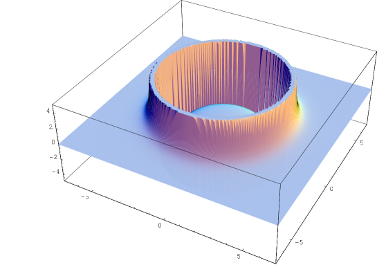
Figure 1: Profile of the Wilson lines in the presence of a puffed brane. The Wilson lines are largest on a ring of radius equal to the gauge-invariant parameter $\beta$.

We will now use the Wilson loops of Ref. [1] to attempt to physically interpret the gauge-invariant parameter $|\beta|$. From now on we will just concentrate on the rank 2 block containing $\beta$. The Wilson loop is

$$e^{\bar{q}C-q\bar{C}}=e^{\bar{q}\alpha-q\bar{\alpha}}\,{\rm cos}(|q|\,\beta)\left(\begin{array}[]{cc}1&\tan(|q|\,\beta)\frac{\bar{q}}{|q|}\\ -\tan(|q|\,\beta)\frac{q}{|q|}&1\end{array}\right).$$ (4.4)

Taking the trace, the (additive) contribution from this block is

$$w(q)=2\,e^{\bar{q}\alpha-q\bar{\alpha}}\,{\rm cos}(|q|\,\beta).$$

According to the Gross-Nekrasov prescription, $q$ should now be identified as a gauge-invariant momentum coordinate for the state described by the Wilson loop. To relate $\beta$ to the position of the vortex, we must first Fourier transform $w(q)$ to position space

$$\hat{w}(x)=\frac{1}{(2\pi)^{2}}\int\,d^{2}q\,w(q)\,e^{i(q\bar{x}+\bar{q}x)}=\frac{2}{(2\pi)^{2}}\int\,d^{2}q\,e^{i(\bar{q}x_{\alpha}+q\bar{x}_{\alpha})}{\rm cos}(|q|\beta)$$ (4.5)

where we have defined the complex position $x_{\alpha}=x-i\alpha$.

Going to polar coordinates $q=\rho\,e^{i\theta}$, $x_{\alpha}=r\,e^{i\phi}$, splitting the cosine in two exponentials, shifting the integration variable $\theta\to\theta+\phi$ and introducing an ${\epsilon}$-cutoff for the radial integration we get

$$\hat{w}(x)=\frac{1}{(2\pi)^{2}}\int d\theta\,\rho\,d\rho\left(e^{[i(r\,{\rm cos}\theta+\beta)-{\epsilon}]\rho}+e^{[i(r\,{\rm cos}\theta-\beta)-{\epsilon}]\rho}\right)$$ (4.6)

Keeping $\epsilon$ only where it is needed, the integral can be evaluated analytically

$$\hat{w}(x)=-\frac{1}{2\pi}\,\frac{\beta}{(\beta+r)^{\frac{3}{2}}}\left(\frac{1}{(\beta-r-i{\epsilon})^{\frac{3}{2}}}+\frac{1}{(\beta-r+i{\epsilon})^{\frac{3}{2}}}\right).$$ (4.7)

Note that this field configuration is real, as it should be, and it is axially-symmetric with respect to the position of the $\beta$-unperturbed vortices $x=i\alpha$. The distribution $\hat{w}(x)$ describes a thin circular shell of radius $\beta$ surrounding the original vortices positions, as seen in Fig. 1. Turning $\beta$ down to zero the shell shrinks and one arrives at the old solution describing two coincident pointlike vortices at $i\alpha$.

Recall that there is a second gauge-invariant definition of the spatial profile of a solution, one may couple the system to fundamental fermion probes and use the profile of the fermion bilinears. If one includes a single additional dimension $z$, then one may probe the system with a 3-dimensional Dirac fermion $\Psi$ with two complex (matrix valued) components $\psi_{1}$ and $\psi_{2}$ which satisfy the Dirac equation

$$\partial_{z}\psi_{1}-C\psi_{2}+\psi_{2}a{}^{\dagger} = 0$$

$$-\partial_{z}\psi_{2}+\overline{C}\psi_{1}-\psi_{1}a = 0.$$ (4.8)

In general a rank $N$ vortex solution has $N$ fermion zero modes if it is independent of the $z$ coordinate. However, as we will explain presently, when $\beta$ is nonzero the equations of motion demand that the vortices always depend on the $z$ coordinate. This lifts some of the fermion zero modes.

For example, in the case of the puffed charged two vortices that we have analyzed, when $\beta$ is nonzero one of the fermion zero modes is unaffected, the generator of the zero-eigenspace of $C$, while the other if lifted. The unaffected fermion is insensitive to $\beta$, and so cannot be used as a probe, it is always equal to the tensor product of the oscillator ground state with a coherent state with coefficient equal to the position of the center of the puffed vortex, so that its bilinear is an eigenstate of the position operator centered in the center of the vortex.

The fate of the lifted zeromode is more interesting. While it is no longer a zeromode, one may find an exact solution to the Dirac equation that describes its evolution in the commutative direction. If, for simplicity, the puffed vortex is centered on the origin, then the individual matrix elements of the fermion are not all coupled in the Dirac equation, they appear in isolated groups of 4, corresponding to various background configurations.

The lifted zeromode only appears in one of these groups. If we write explicitly the matrix form of the components of the Dirac fermion $\Psi$ as

$$\psi_{1,2}=\sum_{q=0}^{\infty}\left(\begin{array}[]{c}\rho_{1,2}^{q}|0\rangle\langle q|\\ \gamma_{1,2}^{q}|1\rangle\langle q|\end{array}\right)$$ (4.11)

then the Dirac equation for the lifted zeromode is simply

$$\partial_{z}\rho^{0}_{1} = \beta\,\gamma^{0}_{2}$$

$$\partial_{z}\gamma_{1}^{1} = \gamma_{2}^{0}$$

$$\partial_{z}\gamma_{2}^{0} = \beta\,\rho_{1}^{0}-\gamma_{1}^{1}.$$ (4.12)

This system of homogeneous linear differential equations is solved by linear combinations of three generalized hypergeometric functions. However no linear combination of these functions appears to be normalizable for the solutions found below, and so we cannot use the locations of the fermion bilinears to define the positions of our solutions, as was possible in the $\beta=0$ case studied by Gross and Nekrasov.

Now that we have understood the meaning of $\beta$, we may attack the problem of its evolution under the equations of motion. Inserting the ansatz (4.1) into the equations of motion, one sees that the $\phi$ equation is unaffected, and the same is true for the $A_{\mu}$’s (if $\beta$ is not real, then one should compensate for its phase with a corresponding pure gauge shift in $A_{\mu}$). The only nontrivial equation is that obtained by varying $C$. Assuming that for $\beta=0$ we have a solution (that is $\Box\alpha=0$), turning on $\beta$ implies the equation

$$\Box\beta+2\beta^{3}=0.$$ (4.13)

We do not know how to solve this equation in general, but we will study two treatable cases.

Figure 2: Time-independent solutions in which the radius $\beta$ depends on a single spatial dimension $x$: they are funnels in which the radius $\beta$ reaches infinity at a finite $x$. These solutions are smooth and describe a vortex ending on a domain wall. These are limits of solutions describing a vortex stretched between two parallel domain walls

First we classify static solutions in which $\beta$ depends only on a single spatial variable $z^{i}=x$. The equation then becomes

$$\frac{d^{2}\beta}{dx^{2}}=2\beta^{3}$$ (4.14)

Bearing in mind that only the modulus of $\beta$ is gauge-invariant, a one parameter family of solutions is given by

$$|\beta(x)|=\frac{1}{|x-x_{0}|}\ .$$ (4.15)

This solution has two distinct branches, one at $x<x_{0}$ and one at $x>x_{0}$, which is depicted in Fig. 2. Each branch describes a D23-brane that ends on a D24.

Another interesting class of solutions arises when we take $\beta$ to be time-dependent ($z^{0}=t$) but spatially homogeneous. In this case the differential equation becomes

$$\frac{d^{2}\beta}{dt^{2}}=-2\beta^{3}.$$ (4.16)

A solution to this equation is given by

$$\beta(t)=a\,{\textrm{dn}}\!\left(a(t-t_{0}),\,2\right)$$ (4.17)

where dn is a Jacobi elliptic function.

This solution looks roughly like a string of ellipsoids attached end to end, although the derivative of $\beta$ is always finite so each intersection is just the union of two opposing cones that touch at their tips, as illustrated in Fig. 3. Each ellipsoid represents a bubble nucleating at some time $t_{0}$, expanding to some maximal size and then decaying back to a point after a period. Note that the Wick rotation of such solutions,

$$\beta(x)=b\,{\textrm{dn}}\!\left(ib(x-x_{0}),\,2\right),$$ (4.18)

gives a real space–dependent solution, which have periodic singularities on an array defined by the initial conditions, the period being $2/bK(-1)$, with $K(q)$ the complete elliptic integral of the first kind. Such extra solutions can be interpreted as D23 branes stretched between two D24’s. On the other hand the special space-solution (4.15), does not admit a real inverse Wick rotation, so it does not generate an extra time dependent solution. Notice moreover that this special solution is obtained from (4.18) by taking $x_{0}=K(-1)/b$, and sending $b\to 0$.

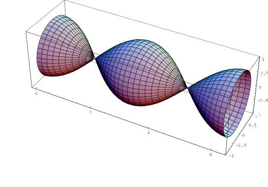
Figure 3: Spatially-homogeneous time-dependent solution describing a braneworld cyclic universe

Such solutions generally have tachyonic instabilities at the tips of the cones, but these are of little concern here as the vortices in this note all suffer from tachyonic instabilities everywhere. They can be stabilized, for example, if one modifies the potential energy so as to spontaneously break the $U(1)$ gauge symmetry at infinity.

Notice that the adjoint scalar plays no role in these vortex solutions, although their forms are fixed by the charge of the vortex. The solutions discussed in this note are therefore also solutions to the pure gauge theory. We expect that many other interesting solutions can be found.

As a side remark we would like to comment on the relation with Open String Field Theory, observing that working at finite $\theta$ seems to mark a profound difference with respect to the infinite noncommutative limit. In particular, at infinite $\theta$ there is a one to one correspondence between noncommutative solitons and String Field Theory solutions [20, 21, 22] (where the string field is basically the noncommutative tachyon). At finite $\theta$, on the other hand, there is no way to get rid of the gauge connection, and the tachyon field plays a minor role (and could be even thrown away without changing the relevant physics). From a formal field theory point of view this is for us no surprise as both the gauge field and the open string field are the connection of two infinite dimensional gauge groups that share lot of similarities [16]. While it is understood that $U(1)$ noncommutative gauge theory is the low energy limit of OSFT on a D25–brane with a constant $B$-field on its worldvolume, it seems that the two theories are very different in the way they are classically solved. It would be therefore interesting to understand the relations (if any) between classical solutions of the two theories, in particular to find the OSFT counterpart of our puffed solutions. It is clear that this question will only be addressable once classical solutions for multiple and lower dimensional D-branes will be understood in OSFT.

Acknowledgments

We would like to express our gratitude to L. Bonora and R. Szabo for carefully reading our manuscript. We also thank G. Barnich, F. Ferrari, C. Krishnan, S. Kuperstein and even D. Persson for enlightening comments and discussions.

N.B. and J.E. are supported in part by a “Pole d’Attraction Interuniversitaire” (Belgium), by IISN-Belgium, convention 4.4505.86, by Proyectos FONDECYT 1970151 and 7960001 (Chile) and by the European Commission program MRTN-CT-2004-005104, in which this author is associated to V.U. Brussels.
C.M. is supported in part by the Belgian Federal Science Policy Office through the Interuniversity Attraction Pole P5/27, in part by the European Commission FP6 RTN programme MRTN-CT-2004-005104 and in part by the “FWO-Vlaanderen” through project G.0428.06.

References

- [1] D. J. Gross and N. A. Nekrasov, “Solitons in Noncommutative Gauge Theory,” arXiv:hep-th/0010090.
- [2] S. Bolognesi, “Domain Walls and Flux Tubes,” arXiv:hep-th/0507273.
- [3] S. Bolognesi, “Large , Strings and Bag Models,” arXiv:hep-th/0507286.
- [4] S. Bolognesi and S. B. Gudnason, “Multi-vortices are Wall Vortices: A Numerical Proof,” arXiv:hep-th/0512132.
- [5] T. Vachaspati and A. Achúcarro, “Semilocal Cosmic Strings,” Phys. Rev. D44 (1991) 3067.
- [6] T. Vachaspati and A. Achúcarro, “Semilocal and Electroweak Strings,” arXiv:hep-th/9904229.
- [7] M. Aganagic, R. Gopakumar, S. Minwalla and A. Strominger, ‘Unstable Solitons in Noncommutative Gauge Theory,” arXiv:hep-th/0009142.
- [8] J. A. Harvey, “Komaba Lectures on Noncommutative Solitons and D-Branes,” arXiv:hep-th/0102076.
- [9] G. Moore and E. Witten, Self-Duality, Ramond-Ramond Fields, and K-Theory, arXiv:hep-th/9912279.
- [10] A. Sen, Tachyon Condensation on the Brane Anti-Brane System, arXiv:hep-th/9805170.
- [11] J. Maldacena, “The Large N Limit of Superconformal Field Theories and Supergravity”, arXiv:hep-th/9711200.
- [12] S.S. Gubser, I.R. Klebanov, and A.M. Polyakov, “Gauge Theory Correlators from Noncritical String Theory,” arXiv:hep-th/9802109.
- [13] E. Witten, “Anti-de Sitter space and Holography,” arXiv:hep-th/9802150.
- [14] R. Gopakumar, S. Minwalla and A. Strominger, “Noncommutative Solitons,” arXiv:hep-th/0003160.
- [15] M. R. Douglas and N. A. Nekrasov, “Noncommutative Field Theory,” arXiv:hep-th/0106048.
- [16] J. A. Harvey, “Topology of the Gauge Group in Noncommutative Gauge Theory,” arXiv:hep-th/0105242.
- [17] R. J. Szabo, “Matrix Models, Large N Limits and Noncommutative Solitons,” arXiv:hep-th/0512068.
- [18] O. Lechtenfeld, A. D. Popov, R. J. Szabo, “Rank Two Quiver Gauge Theory, Graded Connections and Noncommutative Vortices,” arXiv:hep-th/0603232.
- [19] R. Gopakumar, M. Headrick and M. Spradlin, “On Noncommutative Multi-solitons,” arXiv:hep-th/0103256.
- [20] L. Bonora, D. Mamone and M. Salizzoni, “Vacuum string field theory ancestors of the GMS solitons,” arXiv:hep-th/0207044.
- [21] C. Maccaferri, “Chan-Paton factors and higgsing from vacuum string field theory,” arXiv:hep-th/0506213.
- [22] M. Schnabl, “String field theory at large B-field and noncommutative geometry,” arXiv:hep-th/0010034.