The evolution of supersymmetric A-type D-branes under the bulk renormalization group flow between two different $N=2$ minimal models is studied. Using the Landau-Ginzburg description we show that a specific set of branes decouples from the infrared theory, and we make detailed predictions for the behavior of the remaining branes. The Landau-Ginzburg picture is then checked against a direct conformal field theory analysis. In particular we construct a natural index pairing which is preserved by the RG flow, and show that the branes that decouple have vanishing index with the surviving branes.

1 Introduction

Renormalization group flows for perturbed 2d conformal field theories without boundary have been studied in great detail, as have 2d conformal field theories on spaces with boundaries, where the theory is perturbed by a relevant boundary operator. However, the flow of boundary conditions under relevant bulk perturbations is poorly understood, and only specific aspects of some examples have been studied: see [1, 2, 3, 4, 5, 6] for flows to nontrivial IR fixed points, and [7, 8, 9, 10, 11, 12, 13] for massive flows. For exactly marginal bulk perturbations, on the other hand, a general description of the flow of boundary conditions has recently been found in [14]. One may hope that the techniques that were developed there may also shed light on the case with relevant bulk perturbations.

We would expect this problem to have interesting applications in condensed matter physics. It should also be important for string theory. In many cases, renormalization group (RG) flows of worldsheet conformal field theories (CFTs) provide a qualitatively sensible description of the dynamics of tachyon condensation in spacetime (see for example [15, 16] for recent discussions of this point). For closed string tachyons which are not localized, the dilaton initially evolves towards strong coupling [15], indicating that D-branes could be an important part of the dynamics of closed string tachyon condensation.

One particular class of theories where one may hope to be able to address the flow of boundary conditions under bulk perturbations are the 2d unitary minimal models with or without supersymmetry. In these models, there exists only a finite set of boundary conditions which preserve the full (super)conformal symmetry. In the simple example of a charge-conjugation modular invariant these boundary conditions are in one-to-one correspondence with the chiral primaries of the minimal model [18]. As we perturb the theory by a (supersymmetry-preserving) relevant operator, the bulk theory will flow to a minimal model with a smaller central charge for which the number of chiral primaries is smaller. In particular, the number of allowed boundary conditions therefore also decreases. It is then an interesting question to study what happens to the various boundary conditions of the UV theory under the flow. This is essentially the same question, in conformal field theory language, as the one asked in [2].

In this work we shall give an answer for a wide class of RG flows of 2d $N=2$ supersymmetric minimal models with boundary, perturbed by relevant bulk F-terms. There are advantages and disadvantages to studying the flows in this class. The disadvantage is that unlike the case of the non-supersymmetric minimal models, the RG fixed points are separated by an infinite distance as measured by the Zamolodchikov metric [19], so that conformal perturbation theory is not a useful tool. The advantage is that the D-branes which preserve the $N=2$ supersymmetry are governed entirely by the F-terms of the bulk theory, which satisfy non-renormalization theorems that allow one to understand the RG flow completely.

In this paper we shall study the so-called A-type branes that have a very explicit description in terms of the Landau-Ginzburg (LG) analysis of [20]. This will allow us to make quite detailed predictions for the behavior of these branes under the bulk perturbation. We shall find that certain branes flow to superconformal branes of the IR theory, while others decouple. These predictions can be tested against direct conformal field theory arguments, and we find perfect agreement. In particular, inspired by the the Landau-Ginzburg analysis, we identify the RR-charges of the IR theory in terms of the RR-charges of the UV theory. We then construct an index in the UV conformal field theory that only takes into account these IR RR-charges, and that flows to the standard index of [20] in the infrared. It can therefore be used to measure the IR RR-charges of any UV brane; among other things this allows us to distinguish the branes that decouple (and have vanishing index), from those that flow to non-trivial branes in the IR. In addition we are able to study the Affleck-Ludwig $g$-function [21] for the branes which decouple along the flow, and we find that $g$ always tends to zero for them. The physical interpretion of this result is that the corresponding branes decay.

The paper is organized as follows. In §2 we review the $N=2$ minimal models, their RG flows, and the corresponding Landau-Ginzburg (LG) description. In §3 we explain the CFT and LG descriptions of A-type D-branes in minimal models. In §4 we study the bulk RG flows from the point of view of the Landau-Ginzburg theory, and identify which branes decouple in this framework. We also study a number of examples in detail and compute the IR limit of the $N=2$ generalization [20] of the Affleck-Ludwig ‘$g$-function’ [21]. In §5 we analyze the problem using CFT methods. In particular, we construct an index for the D-branes which is preserved along the RG flow. This then allows us (at least for a large class of examples) to confirm the above RG predictions. We conclude in §6 with some remarks on the implications for closed string tachyon dynamics, and a discussion of possible future directions for research. There are two appendices where some of the more technical arguments are described in detail.

2 Review of minimal models

We begin by reviewing some basic facts about $N=2$ minimal models (more precisely, the ‘A series’ of minimal models) and their Landau-Ginzburg description.

2.1 The N=2 superconformal field theory

The holomorphic $N=2$ superconformal algebra is generated by the stress tensor $T(z)$, a $U(1)_{R}$ current $J(z)$, and supersymmetry currents $G^{\pm}(z)$ with $U(1)_{R}$ charges $\pm 1$. For $c\leq 3$ there are a discrete set of unitary ‘minimal models’ at central charge

$$c=\frac{3k}{k+2}\ ,\qquad k=1,2,\ldots\ ,$$ (2.1)

containing a finite number of superconformal primaries. The corresponding (bulk) theories have an A-D-E classification. The theories in the ‘A series’ of the $N=2$ minimal models have the spectrum

$${\cal H}=\bigoplus_{[l,m,s]}{\cal H}_{[l,m,s]}\otimes\overline{{\cal H}}_{[l,-m,-s]}\ ,$$ (2.2)

where the sum runs over all equivalence classes of representations of the coset algebra

$$\frac{{\rm su}(2)_{k}\oplus{\rm u}(1)_{2k+4}}{{\rm u}(1)_{4}}$$ (2.3)

that describes the bosonic subalgebra of the $N=2$ algebra. The representations of (2.3) are labelled by the triples $(l,m,s)$, where $l=0,1,\ldots,k$; $m=0,1,\ldots,2k+3$; and $s=0,1,2,3$. The triples have to satisfy the constraint that $l+m+s$ is even; in addition we have the identification $(l,m,s)\simeq(k-l,m+k+2,s+2)$, where both $m$ and $s$ are being regarded as periodic variables with period $2k+4$ and $4$, respectively. The ground state in ${\cal H}_{[l,m,s]}$ has conformal dimension $h$ and $U(1)_{R}$ charge $q$

$$h=\frac{l(l+2)-m^{2}}{4(k+2)}+\frac{s^{2}}{8}\ \hbox{(mod 1)}\ ;\qquad q=\frac{m}{k+2}-\frac{s}{2}\ \hbox{(mod 1)}\ .$$ (2.4)

The coset representations with $s$ even live in the NS sector, while those with $s$ odd are R-sector representations. In the following the chiral and anti-chiral primaries will also play an important role: in the NS sector, the chiral primaries appear in the sectors $(l,l,0)$ or $(l,-l-2,2)$. The anti-chiral primaries arise for $(l,-l,0)$ or $(l,l+2,2)$. In the R sector, the ground states (or primaries) arise in the sectors $(l,l+1,1)$ or $(l,-l-1,-1)$.

2.2 Landau-Ginzburg description

The A-series minimal models can be described as the IR fixed point of a Landau-Ginzburg theory for a single complex scalar superfield $X$ [23, 24, 25, 26]: in particular, the $k$th minimal model is the IR fixed point of the theory

$${\cal L}_{k}=\int d^{2}x\,d^{2}\theta d^{2}\bar{\theta}\,{\bar{X}}X-\int d^{2}x\,d^{2}\theta\,W(X)+{\rm h.c.}\ ,\qquad W(X)=\frac{\lambda_{k}}{k+2}X^{k+2}\ .$$ (2.5)

The chiral primaries of the theory are simply the bottom components of the superfields $X,X^{2},\ldots X^{k}$ ($X^{k+1}$ is a descendant operator by the equations of motion), with $X^{l}$ corresponding to the operator $(l,l,0)\otimes\overline{(l,-l,0)}$ at the conformal fixed point. The antichiral primaries are labelled by ${\bar{X}}^{l}$ corresponding to $(l,-l,0)\otimes\overline{(l,l,0)}$.

2.3 Renormalization group flows of perturbed minimal models

Next we want to perturb ${\cal L}_{k}$ by the top component of the superfield for a relevant chiral primary

$${\cal L}_{k}\to{\cal L}_{k}-\int d^{2}x\,d^{2}\theta\frac{\lambda_{n}}{n+2}X^{n+2}\ +\ {\rm h.c.}\ ,$$ (2.6)

where $n<k-1$. In terms of the superpotential this simply corresponds to adding to the superpotential of (2.5) the term

$$W(X)=\frac{\lambda_{k}}{k+2}X^{k+2}+\frac{\lambda_{n}}{n+2}X^{n+2}\ .$$ (2.7)

Standard non-renormalization theorems indicate that no additional superpotential terms are induced. Assuming that the kinetic term is in the right universality class, the most relevant coupling $\lambda_{n}$ should dominate, and the theory will flow at low energies to the $n$th minimal model.

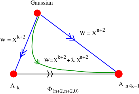
Figure 1: A map of RG flows. The top corner of the triangle denotes the free $c=3$ $N=2$ superconformal theory of a free chiral multiplet $X$. Deforming this theory by the superpotential $W=X^{k+2}$ ($X^{n+2}$) induces a flow to the $k$th ($n$th) minimal model $A_{k}$ ($A_{n}$). Upon a deformation by the relevant chiral primary labelled by $(L,M,S)=(n+2,n+2,0)$, $A_{k}$ flows to $A_{n}$. Finally, the superpotential $W=X^{k+2}+\lambda X^{n+2}$ induces a flow from the free theory which asymptotes to the the flow between the free theory and $A_{k}$ in the UV, and to the flow between $A_{k}$ and $A_{n}$ in the IR.

This flow approximates the flow from the $k$th minimal model in the UV to the $n$th minimal model in the IR, under the perturbation by $(n+2,n+2,0)\otimes\overline{(n+2,-(n+2),0)}$. Strictly speaking, the perturbation (2.7) induces a flow from the free theory in the UV to the $n$th minimal model. However, if $\lambda_{n}$ is small in the UV, the RG flow should begin close to the flow between the free theory and the $k$th minimal model; as $\lambda_{n}$ gets large, the flow starts to run close to the line between the $k$th and $n$th minimal models, as shown in figure 1. In this way we can say that the RG flow of (2.6) approximates the RG flow we are interested in, at least for large $\lambda_{n}$. Note that this basic idea, (and the RG diagram in figure 1) is essentially identical in spirit to the use of gauged linear sigma models for describing the decay of tachyons in non-supersymmetric orbifolds [2, 4, 5]. (Indeed, in those references, the RG flow of these orbifolds is discussed using the mirror of the gauge linear sigma model, which is a 2-field Landau-Ginzburg theory [5, 27, 28].)

In trying to understand the behavior of D-branes under RG flow, we will therefore assume (as do [2, 4, 5]) that studying D-branes in the LG theory (2.7) as $\lambda_{n}\to\infty$ will be a good guide to the behavior of D-branes in the flow between the $N=2$ minimal models $A_{k}$ and $A_{n}$. The essential reasoning is that the D-branes we will be studying are controlled entirely by the F-terms, and the RG flow of these F-terms drives $\lambda_{n}$ to infinity such that it dominates over $\lambda_{k}$ in the infrared. Furthermore, we shall also be able to check at least some of our conclusions against direct conformal field theory arguments, which gives us confidence in our reasoning based on Landau-Ginzburg theory.

3 D-branes in minimal models

In the following we shall study the branes (or boundary conditions) that preserve the full $N=2$ superconformal algebra at the boundary. Such boundary conditions fall into two clases, ‘A-type’ and ‘B-type’ branes, that are distinguished by their gluing condition for the $U(1)_{R}$ current [29]. In this paper we will focus on the ‘A-type’ boundary conditions, as they have a very simple description in the Landau-Ginzburg theory.

3.1 A-type branes in conformal field theory

A-type branes are characterised by the gluing conditions

$$(L_{n}-\bar{L}_{-n})|\!|B\rangle\!\rangle = 0$$

$$(J_{n}+\bar{J}_{-n})|\!|B\rangle\!\rangle = 0$$ (3.1)

$$(G^{\pm}_{r}+i\eta\bar{G}^{\pm}_{-r})|\!|B\rangle\!\rangle = 0\ .$$

Here $\eta=\pm$ corresponds to the two different spin structures; in the following we shall concentrate on one choice of $\eta$, say $\eta=+$.

In conformal field theory these branes are described by their boundary states that can be constructed following Cardy [18]. In each sector of (2.2) there is an Ishibashi state $|l,m,s\rangle\!\rangle$ satisfying (3.1). The consistent boundary states are then labelled by the representations of the coset algebra, i.e. by triples $[L,M,S]$ satisfying the same range (and identifications) as above. Explicitly, the boundary state corresponding to $[L,M,S]$ is given as

$$|\!|L,M,S\rangle\!\rangle=(2k+4)^{-1/4}\sum_{[l,m,s]}\frac{S_{Ll}}{\sqrt{S_{0l}}}\,e^{i\pi\frac{Mm}{k+2}}\,e^{-i\pi\frac{Ss}{2}}\,|l,m,s\rangle\!\rangle\ ,$$ (3.2)

where the sum runs over all equivalence classes of coset representations, and $S_{Ll}$ are the S-matrix elements of SU(2) at level $k$

$$S_{Ll}=\sqrt{\frac{2}{k+2}}\,\sin\left(\pi\,\frac{(L+1)\,(l+1)}{k+2}\right)\,.$$ (3.3)

The two different choices of $\eta=\pm$ correspond now to the different choices $S$ odd or $S$ even. Since we are only interested in one of the two choices we require $S$ to be odd from now on.

The bulk theory (2.2) has RR ground states in the sectors $(l,l+1,1)\otimes\overline{(l,-l-1,-1)}$. For the following it is convenient to normalize these RR ground states as

$$e_{l}=\frac{1}{\sqrt{S_{0l}}}\,(l,l+1,1)\otimes\overline{(l,-l-1,-1)}\ .$$ (3.4)

With this convention the brane denoted by $|\!|L,M,S\rangle\!\rangle$ has charge $Q_{l}(L,M,S)$ with respect to (3.4), where

$$Q_{l}(L,M,S)=\left(\frac{2}{(k+2)^{3}}\right)^{\tfrac{1}{4}}\,\sin\left(\pi\frac{(L+1)(l+1)}{k+2}\right)e^{i\pi\frac{M(l+1)}{k+2}}\,e^{-i\pi\frac{S}{2}}\ .$$ (3.5)

3.2 Landau-Ginzburg description of the A-type branes

As was explained in [20], we can identify the A-type $N=2$ D-branes with directed lines in the complex $X$-plane (where the orientiation corresponds to the sign of the RR charge of the brane). The requirement that the brane preserves A-type supersymmetry implies that $\,{\rm Im}\,W(X)$ is constant along these curves. However, not all such lines are of interest since in general the corresponding brane will have infinite RR charge (and tension). In fact, the $m$’th RR charge of the corresponding D-brane

$$g_{m,k}=\langle X^{m}|B\rangle\!\rangle$$ (3.6)

is a topological quantity [29]. (Here we have denoted a basis of the RR ground states by $X^{m}$, reflecting the fact that the RR ground states which couple to an A-type boundary state are in one-to-one correspondence with the $(c,c)$ chiral ring of the B-twisted theory, generated by the field $X$.) For A-type branes the topological field theory localizes on constant maps into the $X$-plane [20, 29], and this can be used to show [20] that

$$g_{m,k}=N(m,k)\int_{\gamma}dx\,x^{m}\,e^{-W(x)}\ ,$$ (3.7)

where $\gamma$ denotes the curve and $N(m,k)$ is a normalization factor that turns out to be

$$N(m,k)=\frac{1}{\Gamma\left(\frac{m+1}{k+2}\right)}\sqrt{\frac{k+2}{2\sin\left(\frac{\pi(m+1)}{k+2}\right)}}\ .$$ (3.8)

Since this calculates the RR charges of the branes, we should require that $g_{m,k}$ be finite. This implies that $\,{\rm Re}\,W$ must be bounded from below along $\gamma$. In particular, $\gamma$ must pass through a critical point of $W$, i.e. through $x=x_{0}$ with $W^{\prime}(x_{0})=0$. For a homogenous superpotential of the form (2.5) all critical points coincide at the origin. Since $W(0)=0$, the relevant lines have all $\,{\rm Im}\,W=0$. The different curves must therefore run along the lines

$$z=t\,e^{\frac{2\pi ir}{k+2}}\ ,\qquad t\in\mathbb{R}^{+}\ ,\qquad r=0,1\ldots,k+1\ .$$ (3.9)

We will call the brane $(r_{1},r_{2})$ the brane that corresponds to the line for which the orientation is towards the origin along $r_{1}$ and towards infinity along $r_{2}$. This curve corresponds to the A-type brane (3.2) with

$$L+1=|r_{2}-r_{1}|\ ,\qquad M=r_{1}+r_{2}\ ,\qquad S={\rm sign}(r_{2}-r_{1})\ .$$ (3.10)

Note that the pair with the opposite orientation corresponds to the other possible value of $S$; it thus describes the anti-brane. The identification (3.10) was checked in [20] by showing that the RR-charges $Q_{l}(L,M,S)$ agree with the corresponding charges calculated from (3.7).

The geometric interpretation, together with the orientation, makes it clear that we can generate all branes from the $L=0$ branes. That is, consider the branes $(r,r+1)$ and $(r+1,r+2)$. Both branes have a branch which lies along the $z=te^{2\pi i(r+1)/(k+2)}$ line, but with opposite orientation, as seen on the left hand side of figure 2. We expect that in the sum of these branes, a tachyon develops along this line, and that the two branes merge to form the brane $(r,r+2)$, as shown on the right hand side of figure 2. This picture is borne out by an explicit analysis in conformal field theory [30, 31]. In particular, one easily checks that the RR-charges $Q_{l}(L,M,S)$ are preserved along this boundary RG flow.

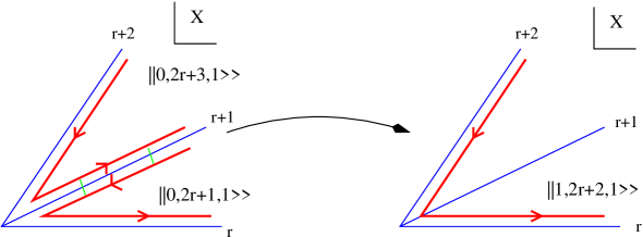
Figure 2: Building all Cardy states from $L=0$ branes. The blue lines labeled $r,r+1,r+2$ are the lines for which $W\in{\mathbb{R}}_{+}$. The red lines, forming wedges between them, are offset slightly so as to make them better visible. On the left they denote two adjacent $L=0$ branes, with the sign of the charge denoted by their orientation. The green lines between these branes are open string tachyons which stretch between branes which lie on the same line but have opposite orientation. The $L=1$ brane on the right is the endpoint of open string tachyon condensation.

3.3 Perturbing the branes

Now we want to consider a perturbation of the form (2.7), as a tool for understanding the behavior of D-branes under RG flow from the minimal model $A_{k}$ in the UV to the minimal model $A_{n}$ in the IR. Our basic philosophy, as discussed in §2.3 above, is that this behavior can be understood by studying D-branes in the $|\lambda_{n}|\to\infty$ limit. At $\lambda_{n}=0$, the branes can be mapped to the minimal model $A_{k}$ describing our UV fixed point, using the techniques of [20].

3.3.1 Some general comments

The claim that we can follow the branes simply by following the contours of constant ${\rm Im}\ W$ as $|\lambda_{n}|\to\infty$ may require some further explanation. First, under RG flow the bulk D-terms also get renormalized; however, as shown in [20], these do not affect the configurations of the A-type branes. Secondly, one may wonder whether any boundary operators are induced along the flow, as in [14, 32, 13]. The non-renormalization theorem for the superpotential also holds for half-superspace integrals on the boundary [33]. Marginal and relevant boundary D-terms, on the other hand, will have the form of gauge field couplings, $A(X)\partial_{0}X$; however, in the present case where we are not including Chan-Paton factors, such terms can be re-written as a gauge-trivial $B$-field coupling in the bulk, which is known not to change the equation ${\rm Im}\ W=0$ for the A-type branes. Furthermore, A-type branes emanating from isolated zeros are rigid, so we do not expect any marginal or relevant operators of the form $T(X)\partial_{1}X$ to be induced on the boundary.

As a further check, if the non-renormalization of the F-terms holds directly in the perturbed minimal models, only D-terms will be induced. However, all of the nontrivial boundary D-terms will be irrelevant. The reason is that they will be of the form $\int d^{2}\theta\Psi$, where $\Psi$ is a superconformal primary field. For minimal models all nontrivial superconformal primaries other than the identity have positive dimension, so the above term in the action will always have dimension greater than $1$. Therefore, in a scheme in which only marginal and relevant couplings are induced by RG flow to the IR, we should not need to consider any boundary terms. This could change if the bulk flow induces irrelevant terms to become relevant, but since the number of superconformal primaries decreases and the spectrum of conformal dimensions remains gapped with only the identity at dimension zero, we believe this will not happen.

3.3.2 Brane decay

When $\lambda_{n}$ is small, we are describing a small perturbation of the UV theory. The asymptotic behavior (for large $x$) of the corresponding curves should not be modified. This implies that each curve must continue to approach two of the UV-lines (3.9) as we go to large $x$. (We shall call the lines (3.9) for the $k$th minimal model the ‘UV-lines’ in the following.) We can thus label each of these curves by a pair $(r_{1},r_{2})$ as above, and for $\lambda_{n}$ small, these lines can again be identified with the branes of the (perturbed) conformal field theory via (3.10).

For each of these curves, $\,{\rm Re}\,W(x)$ increases as $x$ goes to infinity. This implies that the derivative of the real part of $W$ must be zero somewhere along the line, and hence that the line must still go through a critical point of the superpotential $W^{\prime}(x_{0})=0$.

The description above implies that not all combinations of $(r_{1},r_{2})$ will continue to be described by contours of constant ${\rm Im}\ W$ [20]. To see this let us assume that the critical point $x_{0}$ is isolated. $W(x)$ can be approximated as $W(x)=W(x_{0})+\frac{1}{2}W^{\prime\prime}(x_{0})(x-x_{0})^{2}+\cdots$ in the neighborhood of $x_{0}$. There are then two branches with $\,{\rm Im}\,W(x)=\,{\rm Im}\,W(x_{0})$ for which $\,{\rm Re}\,W(x)\geq\,{\rm Re}\,W(x_{0})$ and these describe the brane of interest. Therefore, the asymptotic behavior of the brane is already uniquely determined by the choice of an isolated critical point. For example, if all critical points are isolated, we will only have $k+1$ possible curves, whereas the original unperturbed superpotential had ${k+2\choose 2}$ different curves.

One may thus wonder what happens to the branes of the UV theory that do not satisfy this constraint. At least in the examples we shall study we shall be able to show that any brane of the UV theory can be written as a superposition of branes (in the sense of figure 2) that continue to exist. It is then very plausible to believe that upon switching on the perturbation, a generic UV brane (that cannot continue to exist) will simply decay into a superposition of branes that survive the perturbation, perhaps (for small $\lambda$) still fused together at large $|x|$ by open string tachyons.

In any case, as we switch on the perturbation (2.6) the Landau-Ginzburg description will allow us to analyze the subset of branes of the original $k$th minimal model theory that are still compatible with this constraint. In particular, we can study their behavior as we increase $\lambda_{n}$. This will give us a predicition for how these branes of the $k$th minimal model behave under the RG flow to the $n$th minimal model. This is what we shall be studying in the following. We shall also see that our findings have a natural interpretation in conformal field theory.

3.4 $g$-function

At the conformal fixed point, the $0$’th RR charge is related to the Affleck-Ludwig $g$-function by a phase, $g=|g_{0,k}|$. In boundary conformal field theory, $g$ describes the coupling of the boundary state to the identity, $g=\langle 0|\!|B\rangle\!\rangle$, where $\langle 0|$ is the $SL(2,{\mathbb{C}})$-invariant vacuum in the closed string sector [21]. This measures a regularized dimension of the Hilbert space of open strings beginning and ending on this brane [21, 34]. In string theory compactifications for which the minimal model is a factor of the ‘internal’ part of the CFT (as opposed to the spacetime factor described by a sigma model on ${\mathbb{R}}^{4}$), the 4d graviton will contain the identity operator acting on the minimal model factor, and the $g$-function will compute the tension of the brane in four dimensions [34].

The $g$-function decreases along boundary renormalization group flows [21], and for such flows it evolves via a gradient flow [35]. For relevant bulk perturbations, however, there is no reason to believe such a theorem will hold, and we need to be specific about how we might even define $g$ in such a theory.

On the other hand, since the $g$-function is directly related to the tension of the corresponding brane in string theory, it is important to understand how it behaves under the above RG flows, at least in the IR limit when $|\lambda_{n}|\rightarrow\infty$. When RG flow is interpreted as time evolution (see [15, 16] for reviews and further references), this will be important data for understanding the behavior of D-branes under time evolution.

3.4.1 Definition of the $g$-function

A physically motivated definition, which matches the definition at the bulk conformal point, is the overlap of the boundary state with the properly normalized NS vacuum of the Landau-Ginzburg theory. Similar definitions have appeared in [8, 9, 10, 11] (and an alternative definition proposed in [12].) This NS vacuum is well-defined for any value of the coupling constants $\lambda_{k}$ and $\lambda_{n}$, and it becomes the $SL(2,{\mathbb{C}})$-invariant vacuum at the fixed points of (2.6). In a string theory setting, one may make the perturbed theory physical by coupling it to the spacetime coordinates as in [15]. If the time evolution is not too rapid, we believe that for the NS ground state of the coupled theory, used to define the 4d graviton, the wavefunction in the LG directions will be well-approximated by the wavefunction for the ground state of the LG theory.

Unfortunately, this overlap is quite complicated in general, and one may therefore be tempted to continue using (3.7) for $m=0$, which would be much easier to compute. However, it does not have a clear physical interpretation away from the conformal point. First of all, one should not expect that the tension of the brane (i.e. the coupling to the $SL(2,{\mathbb{C}})$-invariant vacuum in the closed string sector) is directly related to a RR-charge away from the conformal point. Furthermore, we cannot expect that (3.7) continues to make sense for $\lambda_{n}\rightarrow\infty$ since in this limit some of the RR ground states have disappeared altogether.

In order to calculate the $g$-function we therefore need to evaluate the overlap with the ground state. The precise ground state wavefunction is difficult to determine, but we can make some qualitative statements. For example, consider the perturbation (2.6) for large $\lambda_{n}$. In the NS sector, the bosonic potential $|W^{\prime}(X)|^{2}=|X^{k+1}+\lambda X^{n+1}|^{2}$ has its minima at the zeros of $W^{\prime}(X)$. Apart from the $(n+1)$st-order zero at the origin, there are $k-n$ isolated zeros at the solutions of $X_{c}^{k-n}+\lambda_{n}=0$. Fluctuations about these vacua have masses of order $|W^{\prime\prime}(X_{c})|\propto|\lambda_{n}|^{\frac{k}{k-n}}$, which becomes infinite as $|\lambda_{n}|\to\infty$. In the NS sector there are no fermion zero modes. The wavefunctions in field space of the various momentum modes in this massive theory are well-approximated by the wavefunctions for the corresponding simple harmonic oscillator, and their ground state energies will grow with $\lambda_{n}$. Therefore, we expect all of the low-energy states to be concentrated at the origin in $X$-space and die off rapidly away from the origin. The boundary state for any D-branes whose support is far from the origin of $X$-space will thus have vanishingly small overlap with the ground state. For such branes one therefore expects that the $g$-function goes to zero in the limit $|\lambda_{n}|\to\infty$. This suggests that the graviton ceases to couple to these branes. Furthermore all indications are that the RR fields sourced by the branes themselves decouple from the theory [2, 4, 5].

3.4.2 Physical interpretation

However we do not think that the fact that $g\to 0$ for these branes indicates that they become light; in fact, this would be a potential disaster for the theory, as it would mean that any string background which is a possible endpoint of closed string tachyon condensation would have massless nonperturbative objects. Rather, the above discussion indicates that they completely decouple from the excitations described by the infrared conformal field theory. They do not interact with such fields, and we believe they cannot be excited by such fields. For all practical purposes, from the point of view of the observer described by the infrared conformal field theory, the D-branes associated to the critical points moving to infinity have decayed away.

As in [15], this RG analysis will not capture the full time-dependent spacetime process of closed string tachyon decay in the presence of a D-brane, but it should be an important first step in that direction. We close this section by noting to what degree our results are (or are not) similar to the discussions in [6, 13]. We are studying branes that remain attached to massive vacua in the IR, rather than branes which are localized at the tachyon condensate. In the case of [6], this would be like branes localized at the ‘dust vacua’. An analogous setup would be one in which the Riemann surface in [6] is split into two Riemann surfaces, and the observer lives in one component while a D1-brane wraps a 1-cycle in the other component. It seems consistent that such a brane will be seen as having decoupled from the observer. The case of [13] would be most analogous to a perturbation of the form $W=X^{2}$ in our LG picture, for which all of the vacua are massive; our techniques would focus on branes attached to the massive vacua, and would be similar to D0-branes localized at the zeros of the tachyon in [13].

4 Branes in perturbed theories: LG analysis

Now that we have set up the study of supersymmetric boundary conditions in general Landau-Ginzburg models, we can analyze how the above branes behave under the bulk RG flow between minimal models. As we have seen, the A-type supersymmetric branes are determined entirely by the superpotential. We will thus assume that the questions we are asking can be addressed by studying the family (2.7) as one rescales $\lambda_{n}$. It is easy to track the various branes in this family by following the level lines of $\,{\rm Im}\,W$ emanating from the solutions to $W^{\prime}(x)=0$.

In this section we will do this for the case that $n+2$ is a factor of $k+2$. In §5 we will find a clean conformal field theory interpretation of our results in the case that $(k+2)/(n+2)$ is odd.

4.1 Perturbation by $W=X^{(k+2)/d}$

We now want to study the case where we perturb the $k$’th minimal model by the relevant bulk field $X^{n+2}$, where $n+2$ is a factor of $k+2$. The superpotential is thus of the form

$$W(x)=\tfrac{1}{k+2}\,x^{k+2}+\lambda\,\tfrac{d}{k+2}\,x^{\frac{k+2}{d}}\ ,$$ (4.1)

where $d$ is a factor of $k+2$. Part of the reason that this class of examples is particularly easy is that the perturbed theory still has the non-trivial rotation symmetry

$$\rho:x\to e^{\frac{2\pi id}{k+2}}\,x\ .$$ (4.2)

Furthermore, if $\lambda$ is real, the conjugation transformation

$$C:x\to e^{\frac{2\pi id}{k+2}}\,x^{*}$$ (4.3)

is a symmetry of the equations of motion $\,{\rm Im}\,W=0$. We will find that these symmetries cut our workload considerably.

In the following we shall focus on the case $\lambda\in{\mathbb{R}}_{+}$. The structure of the UV and IR branes are as follows. In the limit $\lambda\to 0$ the branes are described by the lines (3.9), while in the limit $\lambda\to\infty$, the branes are described by the IR lines

$$x=te^{\frac{2\pi idr}{k+2}}\ ;\qquad t\in{\mathbb{R}}_{+}\ ,\qquad r=0,1,\ldots,n+1\ .$$ (4.4)

We will also call the wedges between adjacent UV (IR) lines $r,r+1$ the $(r+1)$st ‘UV(IR) wedges’; the branes bounding each UV(IR) wedge are thus the $L=0$ branes in the UV(IR) theory (see figure 3 for an example). Note that the transformation $\rho$ in (4.2) maps the $(r+1)$st IR wedge into the $(r+2)$nd IR wedge.

Let us further denote by $B$ the line which bisects the first IR wedge, i.e. the line with angle $\tfrac{\pi d}{k+2}$. By construction, $W(x)$ is real along $B$ (as well as along the real axis and the other IR lines). The $B$-line will lie on the $d/2$nd UV line when $d$ is even, and it will bisect the $(d+1)/2$nd UV wedge when $d$ is odd. Furthermore, the transformation $C$ (4.3) will flip the $x$-plane around $B$, and maps the first IR wedge back into itself.

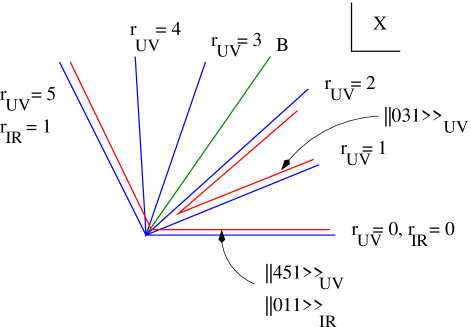
Figure 3: UV and IR lines, and some sample D-branes, for the case $d=5$.

It is now immediate that the IR branes form a subset of the UV branes. In particular some of the curves of the UV theory stay completely fixed upon taking $\lambda\rightarrow\infty$. From the point of view of the Landau-Ginzburg description, the corresponding branes therefore do not change shape under the RG flow (see figure 3 for an example). Translated into conformal field theory language, this then suggests that we have the flow

$$|\!|pd-1,d(p+2q),\pm 1\rangle\!\rangle_{\rm UV}\quad\Longrightarrow\quad|\!|p-1,(p+2q),\pm 1\rangle\!\rangle_{\rm IR}\ ,\qquad p=1,\ldots,n+1\ .$$ (4.5)

We will also find some support for this conjecture in the conformal field theory analysis of §5.

On the other hand, most of the UV branes do not appear in the IR theory since there are more UV lines than IR lines. We wish to understand the fate of the other UV branes as $\lambda\to\infty$. For $\lambda\neq 0$, the critical points of $W$ are at $x=0$ (with multiplicity $n+1$), as well as at the $(k-n)=\tfrac{(k+2)(d-1)}{d}$ points

$$x_{l}=\lambda^{\frac{d}{(k+2)(d-1)}}\,e^{\pi i\frac{d(2l+1)}{(k+2)(d-1)}}\ ,\qquad l=0,\ldots,\frac{(k+2)(d-1)}{d}-1\ .$$ (4.6)

Note that $(d-1)$ of these lie in the interior of each adjacent IR wedge. In particular, $x_{l=0,\ldots,d-2}$ lie in the first IR wedge between $r=0,1$ in (4.4). For future reference we also note that the value of $W$ at these critical points is

$$W(x_{l})=\tfrac{d-1}{k+2}\lambda^{\frac{d}{d-1}}\,e^{\pi i\frac{(2l+1)}{d-1}}\ .$$ (4.7)

Let us focus on the zeros lying within a single IR wedge – by the symmetry $\rho$ (4.2), the story will be identical for the remaining IR wedges. The details of which branes decouple and why depend somewhat on whether $d$ is odd or even. We will describe the general pattern here, and discuss details for the case $d$ odd and even separately below.

Let $\lambda$ have a small imaginary part. In this case, the UV and IR lines deform slightly. The line $B$ defined by ${\rm Im}\ W=0$, which lies in the interior of the IR wedge, then bisects a UV wedge. This is because upon so deforming $\lambda$, no critical point $x_{l}$ will satisfy ${\rm Im}\ W(x_{l})=0$; in particular, $B$ therefore does not go through a critical point, and since ${\rm Re}\ W$ decreases near the origin along $B$, it must continue to do so as $|x|$ becomes large along $B$. The $B$ line therefore cannot asymptote to an UV line along which ${\rm Re}\ W$ increases as $|x|$ becomes large.

In §4.2, §4.3, we shall find that all other UV wedges not bisected by $B$ contain exactly one critical point, and (with the aforementioned deformation of $\lambda$) no critical points lie on a UV line. The branes that emanate from the non-trivial critical points cannot cross $B$ or any of the IR lines (along which we also have that ${\rm Im}\ W=0$) since by the above assumption the value of ${\rm Im}\ W$ at the critical points does not vanish. Furthermore, on all of the UV lines in this region, $W(x)$ is real and positive (for $|x|\rightarrow\infty$), and the phase of $W$ near each line increases (decreases) as the phase of $x$ increases (decreases). Thus ${\rm Im}\ W$ is slightly positive above each UV line, and slightly negative just below each UV line, as illustrated in figure 4. Using these two facts, the results of Appendix A show that every UV $L=0$ brane that asymptotes to the boundary of a wedge containing a critical point, can be generated (by open string tachyon condensation) from branes that decouple.

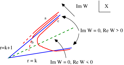
Figure 4: Three contours with constant $\,{\rm Im}\,W$ close to zero. All such contours asymptote to UV lines. Close to the UV lines, ${\rm Im}\ W$ increases as shown. Branes asymptoting from a counterclockwise direction to a UV line have $\,{\rm Im}\,W>0$; branes asymptoting from a clockwise direction have $\,{\rm Im}\,W<0$. In this picture $\,{\rm Im}\,W_{a}>\,{\rm Im}\,W_{b}>\,{\rm Im}\,W_{c}$.

The one $L=0$ brane for which this argument does not apply (and which will in fact not decouple) is the one asymptoting to the boundary of the UV wedge bisected by $B$. Let us call this brane $S$. As we have argued above, the branes associated to the non-trivial critical points decay along the flow. By the same arguments as given below for $d$ odd, one can then show that the UV brane $S$ must flow to the IR $L=0$ brane associated to the IR wedge in question. For example, for the case depicted in figure 3, all of the branes $|\!|0,2p+1,1\rangle\!\rangle_{\rm UV}$ in the first IR wedge will decouple in the IR except for $p=2$. On the other hand, the $L=0$ brane $|\!|0,5,1\rangle\!\rangle_{\rm UV}$ flows to the $L=0$ brane of the IR wedge, i.e. to the brane $|\!|011\rangle\!\rangle_{\rm IR}$.

For $d$ odd, we will find strong evidence in conformal field theory that this picture holds, as we will see in §5. We do not have such an argument for $d$ even, but we suspect that this is just a technical matter.

4.2 The case of odd $d$

From the LG perspective the case where $d$ is odd is simpler since the $B$ line already bisects a UV wedge even for real $\lambda$. The decay picture we have just sketched is then unambiguously defined. [For $d$ even and $\lambda\in{\mathbb{R}}_{+}$, the line $B$ lies on top of the $d/2$nd UV line. If we resolve the situation by making $\lambda$ slightly complex, the UV wedge associated to $S$ depends on the sign of ${\rm Im}\ \lambda$.]

Returning to the case $d$ odd, the critical points $x_{l}$ have the phases

$$\theta=\frac{\pi i}{k+2}\theta_{l}\ ,\qquad\hbox{with}\qquad\theta_{l}=(2l+1)\frac{d}{d-1}\ .$$ (4.8)

These points always lie between adjacent UV lines, since

$$0<\frac{d}{d-1}<2<\frac{3d}{d-1}<4<\frac{5d}{d-1}\cdots\ .$$ (4.9)

The first UV wedge that does not contain a critical point is the $(d+1)/2$nd one, since

$$d-3<\theta_{\frac{d-3}{2}}=\tfrac{(d-2)\,d}{d-1}<d-1<d+1<\theta_{\frac{d-1}{2}}=\tfrac{d^{2}}{d-1}<\ldots\ .$$ (4.10)

Using the transformation $C$ (4.3) it follows that all other UV wedges in the first IR wedge have one and only one critical point in their interior. In fact, this had to be the case since there are $(d-1)$ critical points in the first IR wedge, and $d$ UV wedges, and because the angle between consecutive zeros is greater than the angle between adjacent UV lines (as can be seen from (4.8) and (3.9)). Finally, by the symmetry $\rho$ in eq. (4.2), the same story repeats itself in each IR wedge. The discussion in §4.1, together with the proof in Appendix A, now shows that all of the $L=0$ branes, except for the $L=0$ brane bisected by $B$ and its images under $\rho$, decouple from the IR conformal field theory.

Actually, we can be more explicit and identify concretely which branes emanate from these zeros. Let us concentrate on the critical points between the real axis and $B$; these are the zeros $x_{l}$ with $l=0,\ldots,\tfrac{d-3}{2}=u$. The symmetries $\rho$ and $C$ will tell us what the curves through the other zeros look like. Note that it follows from (4.7) that

$${\rm Im}\ W(x_{l})={\rm Im}\ W(x_{u-l})\ ,\qquad l=0,\ldots,\lfloor\tfrac{u}{2}\rfloor\ .$$ (4.11)

We can prove (see appendix B) and have verified by numerical computation for $d\leq 13$ the following geometric picture for the branes emanating from $x_{l}$. The curve for $l=0$ asymptotes to the zero’th and first UV line, i.e. it corresponds to the brane $|\!|0,1,\pm 1\rangle\!\rangle_{\rm UV}$ in conformal field theory. The curve through the critical point for $l=u=\tfrac{d-3}{2}$ asymptotes in one direction to the $\tfrac{d-1}{2}$th UV line. In the opposite direction it goes to the critical point $l=0$; because of (4.11) the imaginary parts of $W$ agree and $\,{\rm Re}\,W(x_{u})<\,{\rm Re}\,W(x_{0})$. From there the brane may take either branch of the brane through $x_{0}$, i.e. either branch of $|\!|011\rangle\!\rangle_{UV}$. If we give $\lambda$ a small positive imaginary part, ${\rm Im}\ W(x_{u})<{\rm Im}\ W(x_{0})$. The contours now cannot cross; furthermore, given the discussion in the previous section and appendix B, the line from $x_{u}$ must asymptote to either the 0th or 1st UV line slightly counterclockwise from the brane emanating from $x_{0}$. Therefore, it must asymptote to the real axis, and hence correspond to the brane $|\!|u,u+1,\pm 1\rangle\!\rangle_{\rm UV}$ in conformal field theory.

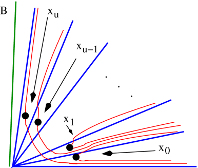
Figure 5: A picture of the decoupling branes for $d$ odd when ${\rm Im}\ \lambda>0$.

Continuing in this fashion, we have found that the curve through $l=1$ asymptotes to the first and second UV line, i.e. it corresponds to $|\!|0,3,\pm 1\rangle\!\rangle_{\rm UV}$ in conformal field theory. The line through $l=u-1$ on the other hand asymptotes in one direction to the $\tfrac{d-3}{2}$nd UV line, and joins the $l=1$ critical point in the other; as before, if we give $\lambda$ a small positive imaginary part, it will continue along the first UV line, and hence correspond to $|\!|\tfrac{d-7}{2},\tfrac{d-1}{2},\pm 1\rangle\!\rangle_{\rm UV}$ in conformal field theory. The curves that go through these critical points thus correspond to the UV branes

$$|\!|0,2l+1,\pm 1\rangle\!\rangle_{\rm UV}\qquad l=0,\ldots,\lfloor\tfrac{u}{2}\rfloor$$ (4.12)

$$|\!|2l-u,u+1,\pm 1\rangle\!\rangle_{\rm UV}\qquad l=\lfloor\tfrac{u}{2}\rfloor+1,\ldots,u\ ,$$

where as before $u=\tfrac{d-3}{2}$. As $\lambda\to\infty$, all of these curves move away from the origin in $x$-space. Since $g\to 0$ in this limit, they completely decouple from the IR theory and can be treated as having decayed away. The same is true for the branes between $B$ and the first IR line, as can be shown using the transformation $C$ in (4.3).

From these decoupling branes (4.12) we can construct, using open string tachyon condensation, all of the $L=0$ branes $|\!|0,2p+1,\pm 1\rangle\!\rangle_{\rm UV}$ with $p=0,1,\ldots,\tfrac{d-3}{2}$, i.e. all the $L=0$ branes between the real axis and $B$. Similarly, from the images of (4.12) under $C$ we obtain the $L=0$ branes between $B$ and the first IR line: $|\!|0,2p+1,\pm 1\rangle\!\rangle_{\rm UV}$ with $p=\tfrac{d+1}{2},\ldots,d-1$. Assuming that the open string tachyon condensation does not significantly change the RG behavior of the component branes, we can thus conclude that all such $L=0$ branes decouple. As we shall see this will be in agreement with the conformal field theory index calculation of §5.

On the other hand, there is one UV $L=0$ brane in the first IR wedge for which this argument does not apply, namely $|\!|0,d,1\rangle\!\rangle_{\rm UV}$ which asymptotes to the two neighboring UV lines that are separated by $B$. To determine what this brane flows to we observe that we can write the UV brane $|\!|d-1,d,1\rangle\!\rangle_{\rm UV}$ asymptoting to the first 2 IR lines as the sum

$$|\!|d-1,d,1\rangle\!\rangle_{\rm UV}=|\!|0,d,1\rangle\!\rangle_{\rm UV}+\sum_{p=0}^{\frac{d-3}{2}}|\!|0,2p+1,1\rangle\!\rangle_{\rm UV}+\sum_{p=\frac{d+1}{2}}^{d-1}|\!|0,2p+1,1\rangle\!\rangle_{\rm UV}\ .$$ (4.13)

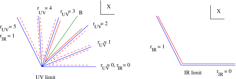
Figure 6: The flow of D-branes for the case $d=5$. On the left-hand-side, the dashed lines correspond to $L=0$ branes which decouple, while the $L=0$ UV brane bisected by $B$ flows to the IR brane $|\!|011\rangle\!\rangle_{\rm IR}$.

Because of the above results, the branes in the two sums on the right hand side of (4.13) all decouple. The brane on the left hand side flows as in (4.5). If we assume that open string tachyon condensation does not modify the behavior under the bulk flow, we conclude that $|\!|0,d,1\rangle\!\rangle_{\rm UV}$ flows as

$$|\!|0,d,1\rangle\!\rangle_{\rm UV}\Longrightarrow|\!|0,1,1\rangle\!\rangle_{\rm IR}\ .$$ (4.14)

More generally,

$$|\!|0,d(2r+1),1\rangle\!\rangle_{\rm UV}\Longrightarrow|\!|0,(2r+1),1\rangle\!\rangle_{\rm IR}\ ,\qquad r\in{\mathbb{Z}}\ ,$$ (4.15)

where we have used the symmetry $\rho$ to obtain the result for the cases with $r\neq 0$. In section §5 we will reproduce this result using conformal field theory arguments.

4.2.1 Example: $d=5$

To illustrate these ideas, let us consider the explicit example with $d=5$. In this case $u=1$, and there are two UV wedges between $B$ and the real axis, and two corresponding critical points, $x_{0}$ and $x_{1}$. Figure 7 shows a numerical plot of the curves emanating from these two critical points, when $\lambda$ has phase $e^{i\pi/10}$ (i.e. a small positive imaginary part). The brane emanating from $x_{0}$ corresponds to the deformation of the Cardy state $|\!|0,1,1\rangle\!\rangle_{\rm UV}$, while the brane emanating from $x_{1}$ corresponds to $|\!|1,2,1\rangle\!\rangle_{\rm UV}$. Note that we can write both $L=0$ branes by subtracting the first brane from the second and condensing the corresponding open string tachyon: $|\!|0,3,1\rangle\!\rangle_{\rm UV}=|\!|1,2,1\rangle\!\rangle_{\rm UV}-|\!|0,1,1\rangle\!\rangle_{\rm UV}$.

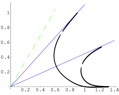
Figure 7: The decoupling branes in the case $d=5$ between the real axis and $B$, where $\lambda$ is given a small imaginary part. The dashed green line corresponds to $B$, the horizontal axis is the real axis, and the vertical axis is the imaginary axis. The other two straight lines are the first and second UV lines $r=1,2$. The curve between the first UV line and the real axis is the deformation of $|\!|0,1,1\rangle\!\rangle_{\rm UV}$, and the curve between the real axis and the second UV line is the deformation of $|\!|1,2,1\rangle\!\rangle_{\rm UV}$. The critical points $x_{0,1}$ lie in the breaks of the curves.

We have also studied numerically the curves between $B$ and the first IR line. When $\lambda$ has a small positive imaginary part, the transformation $C$ is no longer a symmetry of the equations of motion – rather, it takes $\lambda\to\lambda^{*}$. For ${\rm Im}\ \lambda>0$, the transformation $C$ maps these branes to the branes for the theory with coupling $\lambda^{*}$ (for which ${\rm Im}\ \lambda^{*}<0$), between the real axis and $B$. Indeed, we find that the the corresponding branes correspond to $|\!|0,7,1\rangle\!\rangle_{\rm UV}$ and $|\!|0,9,1\rangle\!\rangle_{\rm UV}$. Therefore, as discussed above, all of the $L=0$ branes between the real axis and the first IR line, except for $|\!|0,5,1\rangle\!\rangle_{\rm UV}$, are generated. The UV brane $|\!|4,5,1\rangle\!\rangle_{\rm UV}$ coincides with the IR brane $|\!|0,1,1\rangle\!\rangle_{\rm IR}$ as in (4.5). Following (4.13), the UV brane $|\!|0,5,1\rangle\!\rangle_{\rm UV}$ can be written in terms of the decoupling branes as:

$$|\!|0,5,1\rangle\!\rangle_{\rm UV} = |\!|4,5,1\rangle\!\rangle_{\rm UV}-|\!|1,2,1\rangle\!\rangle_{\rm UV}-|\!|0,7,1\rangle\!\rangle_{\rm UV}-|\!|0,9,1\rangle\!\rangle_{\rm UV}$$

$$= |\!|4,5,1\rangle\!\rangle_{\rm UV}-|\!|0,1,1\rangle\!\rangle_{\rm UV}-|\!|0,3,1\rangle\!\rangle_{\rm UV}-|\!|0,7,1\rangle\!\rangle_{\rm UV}-|\!|0,9,1\rangle\!\rangle_{\rm UV}\ .$$

All of the $L=0$ and $L=1$ UV branes on the right hand side decouple, while we have $|\!|4,5,1\rangle\!\rangle_{\rm UV}\Longrightarrow\ |\!|0,1,1\rangle\!\rangle_{\rm IR}$, and hence deduce that $|\!|0,5,1\rangle\!\rangle_{\rm UV}\Longrightarrow|\!|0,1,1\rangle\!\rangle_{\rm IR}$ as well.

4.3 Even $d$

The case of $d$ even is quite similar. However, we do not yet have a clear CFT picture of this case, so we will be quite brief.

When $\lambda\in{\mathbb{R}}$, the line $B$ and the critical point $x_{\frac{d}{2}-1}$ lie on the $d/2$nd UV line. This is a degenerate situation – the brane emanating from this critical point lies along $B$, and upon reaching the origin will continue along either the real axis or the first IR line. The degeneracy can be split by giving $\lambda$ a small imaginary part. If $\lambda$ has a small positive imaginary part, the line $B$ defined by ${\rm Im}\ W=0$ shifts clockwise and bisects the $d/2$nd UV wedge. On the other hand, if we give $\lambda$ a small imaginary negative part, $B$ bisects the $(\frac{d}{2}+1)$st UV wedge. In either case, the critical point $x_{\frac{d}{2}-1}$ moves off the $d/2$nd UV line, and then it follows from the same arguments as at the beginning of section §4.2 that all UV wedges, except for the UV wedge bisected by $B$, contain precisely one critical point.

At this point we can appeal to the proof in appendix A to make the following claim. For ${\rm Im}\ \lambda$ small and positive, all of the branes $|\!|0,2p+1,\pm 1\rangle\!\rangle_{\rm UV}$ decouple except for the brane $|\!|0,d-1,\pm 1\rangle\!\rangle_{\rm UV}$. The UV brane $|\!|d-1,d,\pm 1\rangle\!\rangle_{\rm UV}$ asymptotes to the real axis and the first IR line, and is expected to flow to $|\!|0,1,1\rangle\!\rangle_{\rm IR}$. Since this UV brane is a sum of all of the UV branes between the real axis and the first IR line, we also expect that $|\!|0,d-1,1\rangle\!\rangle_{\rm UV}\Longrightarrow|\!|0,1,1\rangle\!\rangle_{\rm IR}$.

If $\lambda$ has a small negative imaginary part, all of the $L=0$ branes except for $|\!|0,d+1,1\rangle\!\rangle_{\rm UV}$ are expected to decouple, and we expect that $|\!|0,d+1,\pm 1\rangle\!\rangle_{\rm UV}\Longrightarrow|\!|0,1,1\rangle\!\rangle_{\rm IR}$.

5 D-branes in perturbed minimal models

As discussed in §2.3, the LG flow of the action (2.6) approximates the flow between the minimal models we are interested in. We therefore expect that our results about the behavior of the branes under the LG flow apply directly to the flow between these two conformal field theories. In this section we will check our conjectures for the branes discussed in §4.2 ($d$ odd) directly using conformal field theory methods.

The superpotential (4.1) should describe the flow between the $k$’th minimal model and the $n$’th minimal model that is induced by the relevant bulk operator from the NS-NS sector

$$(n+2,n+2,0)\otimes\overline{(n+2,-(n+2),0)}\ ,$$ (5.1)

as well as its complex conjugate, the (ac) field

$$(n+2,-(n+2)),0)\otimes\overline{(n+2,n+2,0)}\ .$$ (5.2)

As we have argued above, the LG analysis suggests that we have the flow (4.5). We shall now attempt to give some support for this statement from a conformal field theory point of view. We will do this by computing the conserved RR charges of various D-branes, and by constructing a supersymmetric ‘index’ in the UV theory which flows to the index of [20] in the IR theory.

First we observe that the UV branes that appear on the left-hand-side of (4.5), i.e. the special branes

$$|\!|pd-1,d(p+2q),\pm 1\rangle\!\rangle_{\rm UV}$$ (5.3)

have the property that their RR charges (3.5) satisfy (recall that $n+2=\tfrac{k+2}{d}$)

$$Q_{l+(n+2)}(pd-1,d(p+2q),\pm 1)=Q_{l}(pd-1,d(p+2q),\pm 1)\ ,\qquad l=0,\ldots,k-(n+2)$$ (5.4)

and

$$Q_{r(n+2)-1}(pd-1,d(p+2q),\pm 1)=0\ ,\qquad r=1,\ldots,d-1\ .$$ (5.5)

Thus they only couple to $n+1$ different linear combinations of RR charges. Furthermore, we have that

$$Q_{l}(pd-1,d(p+2q),\pm 1)_{\rm UV}={\cal N}\,Q_{l}(p-1,p+2q,\pm 1)_{\rm IR}\ ,\qquad l=0,\ldots,n\ ,$$ (5.6)

where ${\cal N}$ is a constant (independent of $l$), and the charges on the right hand side refer to the IR theory. This is obviously in perfect agreement with the proposed flow (4.5).

There is yet another point of view from which this is very natural. In the original UV theory the different RR ground states $e_{l}$ (3.4) all have degenerate conformal weight equal to the minimal value $h=\bar{h}=\tfrac{c}{24}$. As we consider the perturbation by the NS-NS fields (5.1) and (5.2), the eigenstates of lowest conformal weight (that will correspond to the RR ground states in the IR) will generically be linear combinations of RR ground states that are related to one another by successive fusions with (5.1) and (5.2). Now under successive fusion with the (ca) and (ac) fields (5.1) and (5.2), the RR ground states corresponding to $l+(n+2),l+2(n+2),\ldots,l+(d-1)(n+2)$ for $l=0,\ldots,n+1$ get mixed together. Generically, such a mixing will lift the degeneracy in conformal weight. One should thus expect that only one linear combination of these RR ground states will continue to have minimal conformal weight, while the conformal weight of the other eigenstates will be bigger. The eigenstate with minimal conformal weight is then the only state that can become the RR ground state of the IR theory. This is in very nice agreement with the above.

5.1 Definition of the index

We now want to make a prediction for what happens to the other branes, in particular the UV branes with $L=0$. The above analysis suggests an identification of the RR ground states of the IR theory with specific linear combinations of RR ground states of the UV theory. With this idea in mind, we should now be able to determine the IR RR charges of any UV brane; in particular, this can be done using the index (that calculates an appropriate inner product of the RR ground states). We do this by studying analogs of the index pairing of [20].

In the UV theory, the index is defined by [20] (see also [36]):

$${\cal I}\Bigl{(}|\!|L_{1},M_{1},S_{1}\rangle\!\rangle,|\!|L_{2},M_{2},S_{2}\rangle\!\rangle\Bigr{)}=(-1)^{\frac{S_{1}-S_{2}}{2}}\,\left\{\begin{array}[]{cl}N_{L_{1}L_{2}}{}^{\Delta M}&\hbox{if $0\leq\Delta M\leq k$}\\ -N_{L_{1}L_{2}}{}^{-\Delta M-2}&\hbox{if $-k-2\leq\Delta M\leq-2$}\\ 0&\hbox{if $\Delta M=-1,k+1$}\ .\end{array}\right.$$ (5.7)

Here $N_{L_{1}L_{2}}{}^{l}$ is the su$(2)_{k}$ fusion matrix, $\Delta M=M_{2}-M_{1}$, and $S_{1}$ and $S_{2}$ are both odd. This index is not symmetric, but it is rather obtained from a symmetric inner product upon applying the spectral flow operator to one of the two branes; indeed if we denote by $\langle\cdot,\cdot\rangle$ the symmetric inner product (that is obtained from the usual orthogonal inner product on the RR ground states) then we have

$${\cal I}\Bigl{(}|\!|L_{1},M_{1},S_{1}\rangle\!\rangle,|\!|L_{2},M_{2},S_{2}\rangle\!\rangle\Bigr{)}=\Bigl{\langle}|\!|L_{1},M_{1},S_{1}\rangle\!\rangle,|\!|L_{2},M_{2}+1,S_{2}+1\rangle\!\rangle\Bigr{\rangle}\ .$$ (5.8)

Incidentally, this is the reason for why the index is not symmetric, but instead satisfies

$${\cal I}\Bigl{(}|\!|L_{1},M_{1},S_{1}\rangle\!\rangle,|\!|L_{2},M_{2},S_{2}\rangle\!\rangle\Bigr{)}={\cal I}\Bigl{(}|\!|L_{2},M_{2}+2,S_{2}+2\rangle\!\rangle,|\!|L_{1},M_{1},S_{1}\rangle\!\rangle\Bigr{)}\ .$$ (5.9)

In the application we have in mind, we want to calculate the index that is relevant to the IR theory, but evaluate it in the UV theory. One may therefore guess that the relevant spectral flow operator that enters the index should be the one that is appropriate for the IR theory, rather than the UV theory. At least for $d$ odd this is well-defined; we therefore propose that the index we should use is

$$\widehat{\cal I}^{(d)}\Bigl{(}|\!|L_{1},M_{1},S_{1}\rangle\!\rangle,|\!|L_{2},M_{2},S_{2}\rangle\!\rangle\Bigr{)} = \Bigl{\langle}|\!|L_{1},M_{1},S_{1}\rangle\!\rangle,|\!|L_{2},M_{2}+d,S_{2}+d\rangle\!\rangle\Bigr{\rangle}$$

$$= {\cal I}\Bigl{(}|\!|L_{1},M_{1},S_{1}\rangle\!\rangle,|\!|L_{2},M_{2}+d-1,S_{2}+d-1\rangle\!\rangle\Bigr{)}\ .$$

The index is thus given by the same formula as (5.7), except that now $\Delta M$ is replaced by $\hat{\Delta}M=M_{2}+d-1-M_{1}$.

The index between the special UV branes (5.3) and the $L=0$ branes is

$$\widehat{\cal I}^{(d)}\Bigl{(}|\!|pd-1,d(p+2q),\pm 1\rangle\!\rangle,|\!|0,M,1\rangle\!\rangle\Bigr{)}=0\qquad\hbox{unless $M=d(2r+1)$}\ .$$ (5.11)

Note that this conclusion is actually independent of the order in which we consider the two branes. If $M=d(2r+1)$, we find

$$\widehat{\cal I}^{(d)}\Bigl{(}|\!|pd-1,d(p+2q),1\rangle\!\rangle,|\!|0,d(2r+1),1\rangle\!\rangle\Bigr{)}=\epsilon\left(\delta_{r,p+q-1}-\delta_{r,q-1}\right)\ ,$$ (5.12)

where $\epsilon$ is an irrelevant sign. This should be matched by the index in the IR, for which we have

$${\cal I}_{\rm IR}\Bigl{(}|\!|p-1,(p+2q),\pm 1\rangle\!\rangle,|\!|0,2r+1,1\rangle\!\rangle\Bigr{)}=\left(\delta_{r,p+q-1}-\delta_{r,q-1}\right)\ .$$ (5.13)

Thus this suggests the flow

$$|\!|0,d(2r+1),1\rangle\!\rangle_{\rm UV}\quad\Longrightarrow\quad|\!|0,(2r+1),1\rangle\!\rangle_{\rm IR}\ ,$$ (5.14)

while all other UV branes with $L=0$ decouple. This rule is in perfect accord with the results of §4.2, in particular with eq. (4.15).

This arguments bears some relation to the discussion in [4] (see also [37]). In that work the authors construct an index pairing, representing the intersection matrix for fractional branes in a non-supersymmetric orbifold with tachyons; and an intersection matrix for the D-branes of the theory described by the condensation of twisted sector tachyons. They then construct a transformation which embeds the latter as a block-submatrix of the former; the other block represents the intersection matrix of the ‘Coulomb branch branes’ which decouple from the infrared CFT and which bear a strong resemblance to the decoupling branes in our work (indeed, they are mirror to A-type branes in a Landau-Ginzburg theory). In this section, however, we have provided a construction of a pairing in the UV theory directly from a worldsheet point of view, using the structure of the $N=2$ superconformal algebra. This pairing flows to the index in the IR, and we have used it to correctly deduce which branes of the UV theory will decouple in the IR.

6 Conclusions

In this paper we have determined the behavior of the $N=2$ A-type branes under a bulk flow from the $k$th minimal model to the $n$th minimal model (where $d=\tfrac{k+2}{n+2}$ is an integer). In particular, we have given good evidence, combining the LG analysis with conformal field theory arguments, that some of the superconformal branes of the UV decouple, while others flow to the superconformal A-type branes of the IR theory. For $d$ odd and real coupling constant $\lambda$, the flow behavior could be very explicitly described — see in particular (4.15). Using successive open string tachyon condensation (as for example used in §4.2) this rule then determines the fate of every superconformal UV brane under the flow. As far as we are aware, this is the first time that the behavior of D-branes under a relevant bulk flow could be determined in such detail.

There are a number of natural directions in which to extend this work. First of all, there are a few technical points that deserve further exploration: for example, it would be interesting to find a CFT argument for $d$ even; it would be nice to work out the analysis for the case when $n+2$ is not a factor of $k+2$ — probably at least the LG arguments of §4.1 will generalize fairly straightforwardly to the general situation; it would also be good to apply the same analysis to the D- or E-models (for which everything should go through). More generally, it would be interesting to study the fate of the ‘B-type’ branes in this class of RG flows. The CFT arguments should be quite similar, but the Landau-Ginzburg description of B-type branes is rather different since they correspond to matrix factorizations [38, 39, 40] about which much has been learned in recent years. For the example of the A-models that has concerned us here, the results of [41] should in particular be useful. Another interesting exercise would be to study flows in other models in which we have some control, such as the $N=2$ coset models in [42], which have a Landau-Ginzburg description.

While the $N=2$ RG flows travel an infinite distance with respect to the Zamolodchikov metric, the $N=0$ minimal models with $c=1-\delta$, $\delta\ll 1$ contain both bulk and boundary flows to neighboring fixed points which are treatable within conformal perturbation theory [23]. The fate of D-branes in these models under relevant boundary flows has been studied in [43], and a generalization of the ‘absorption of boundary spin’ principle of [44] has been given for spin-current couplings in more general coset models in [45]. It would be interesting to study the fate of boundary conditions under bulk flows using such techniques. In particular, in a Lagrangian formulation we would wish to compute the beta functions for coupled bulk and boundary flows, as in [14, 32, 13], and understand how the D-branes evolve.

Finally, we would like to understand better the implications of this work for time-dependent string theory backgrounds with D-branes.

Appendix A Generating all of the decoupling branes

In this appendix we want to show that the decoupling branes generate all the $L=0$ charges, except for the $L=0$ brane that is bisected by $B$. In order for this to make sense we want to make sure that $B$ does not lie on top of a UV line, and that the values of ${\rm Im}\ W$ at the different critical points are distinct. For $d$ even or odd, this is achieved by giving $\lambda$ a small imaginary part.

We begin by proving the following statement:

Claim 1. For every UV line between two adjacent IR lines there is at least one decoupling brane (i.e. a brane whose corresponding line emanates from a non-trivial critical point) that asymptotes to the given UV line.

Proof: Let us denote the number of UV lines that lie between $B$ and the IR line asymptoting to the real axis by $m+1$. These lines bound $m$ UV wedges that lie entirely between $B$ and the IR line, and each of these wegdes contains precisely one critical point of $W$. (This follows from the above assumption.) We will label the critical points by $x_{1},\ldots,x_{m}$, ordered such that $\,{\rm Im}\,W(x_{1})<\,{\rm Im}\,W(x_{2})<\cdots<\,{\rm Im}\,W(x_{m})$. We claim that the non-intersecting level lines through $x_{1},\ldots x_{m}$ will asymptote to at least $m+1$ UV lines. The argument will be identical for the branes between $B$ and the first IR line. The images of these branes under $\rho$ will finally complete the picture.

Let us label the UV lines in an anticlockwise order by $L_{1},\ldots,L_{r}$. A given configuration of level lines is described as follows. For each $L_{i}$ let $\Delta_{i}$ be the ordered set of lines that asymptote to $L_{i}$ where the order corresponds to the anti-clockwise order in which the lines approach $L_{i}$. We may denote the lines by the critical points through which they pass; then the order of lines in $\Delta_{i}$ is the same as the increasing order of the points $x_{j}$, and for large $|x|$ is the increasing order of the corresponding contours in a counterclockwise direction (see figure 4). We may thus formally write $\Delta_{j}$ as the product

$$\Delta_{j}=x_{s_{1}}x_{s_{2}}\cdots x_{s_{n}}\qquad\hbox{with $x_{s_{1}}<x_{s_{2}}<\cdots<x_{s_{n}}$.}$$

The condition that these lines form a consistent configuration (i.e. that they do not intersect) can now be formulated as follows: consider the free group generated by the $x_{k}$ subject to the relations $x_{k}^{2}=1$. Then the configuration is consistent if the group element

$$\Delta_{1}\,\Delta_{2}\,\cdots\,\Delta_{r}=1$$ (A.1)

in the group. To understand this, note that if $x_{s}$ appears to the right of $x_{r}$ in (A.1), then the large-$x$ limit of the corresponding contour passing through $x_{s}$ lies counterclockwise to the large-$x$ limit of the contour passing through $x_{r}$. Each group element $x_{k}$ appears twice in (A.1), as each brane has two branches. Since the contours may not cross, we may never have a sequence $x_{s}\ldots x_{r}\ldots x_{s}\ldots x_{r}$. The allowed ordering is: $x_{s}\ldots x_{r}\ldots x_{r}\ldots x_{s}$, $x_{s},\ldots x_{s},\ldots x_{r},\ldots x_{r}$, or the same with $x_{s}\leftrightarrow x_{r}$. For $m$ finite this means that one will eventually find at least one $x_{t}$ adjacent to the second occurrence of $x_{t}$ in (A.1). Using the relations, these can be removed and the process continued – the result will be that all pairs are replaced by the identity, using the relations.

Any consistent configuration is essentially uniquely characterised by the product of the $x_{k}$ (without reference to the $\Delta_{j}$): given any product of $x_{k}$, we collect all increasing elements in $\Delta_{1}$, the next sequence of increasing elements in $\Delta_{2}$, etc. This is then also a consistent configuration and it involves, if anything, fewer UV lines (i.e. fewer $\Delta_{j}$) than the original configuration. So for example, for the sequence

$$123443566521$$

we take

$$\Delta_{1}=\{1234\}\ ,\ \ \Delta_{2}=\{4\}\ ,\ \ \Delta_{3}=\{356\}\ ,\ \ \Delta_{4}=\{6\}\ ,\ \ \Delta_{5}=\{5\}\ ,\ \ \Delta_{6}=\{2\}\ ,\ \ \Delta_{7}=\{1\}\ .$$

Thus we have reduced the problem to proving that (A.1) implies that there are at least $r=m+1$ sets of increasing sequences. This can be proved by induction on $m$.

The first step of the induction is obvious by inspection. Next, assume that we have proven the statement for all sequences of pairs of $x_{k}$, subject to the constraints above, with $k=1,\ldots,m\leq m_{0}-1$. Now consider a group element (A.1) involving the $m_{0}$ different $x_{k}$, $k=1,\ldots,m_{0}$. We concentrate on the two elements $x_{m_{0}}$ that appear in (A.1). There are two cases to consider.

If the two $x_{m_{0}}$ are adjacent in (A.1), it is clear that the second $x_{m_{0}}$ makes up a $\Delta$ by itself. Thus if we remove the two $x_{m_{0}}$ we reduce the number of $\Delta$s at least by one; the induction hypothesis then implies that the number of $\Delta_{j}$ must have been at least $m_{0}+1$.

In the other case, the two $x_{m_{0}}$ do not stand next to each other. Then the group element in question must be of the form

$$g_{1}\,x_{m_{0}}\,h\,x_{m_{0}}\,g_{1}^{-1}\ .$$ (A.2)

In order for this to be the identity it follows that $h$ must be the identity (in the free group involving $r_{h}$ elements) and that $g_{1}$ and $g_{1}^{-1}$ can only involve the other $m_{0}-1-r_{h}$ elements. By the induction hypothesis, $h$ involves at least $r_{h}+1$ $\Delta$s. Similarly, the product $g_{1}g_{1}^{-1}$ involves at least $m_{0}-r_{h}$ $\Delta$s. The first $x_{m_{0}}$ can always be adjoined to the last $\Delta_{j}$ of $g_{1}$ (and it will guarantee that the first element of $h$ will lie in a new $\Delta$), while the second $x_{m_{0}}$ can always be adjoined to the last $\Delta_{j}$ of $h$ (and it will guarantee that the first element of $g_{1}^{-1}$ will again lie in a new $\Delta$). Thus it follows that the total number of $\Delta$s of (A.2) is at least

$$(r_{h}+1)+(m_{0}-r_{h})=m_{0}+1\ ,$$

proving our claim. QED.

Next, we wish to show that all of the $L=0$ branes between $B$ and an IR line can be generated from the decoupling branes. To see this we first prove:

Claim 2. Suppose that there exists for each $\Delta_{k}$ an ascending sequence $(\Delta_{k})=x_{s^{k}_{1}}\cdots x_{s^{k}_{r}}$, where $k_{i}\in\{1,\ldots,m\}$ such that

$$(\Delta_{1})\cdots(\Delta_{m+1})=1\ .$$ (A.3)

[Note that it follows from Claim 1 that every consistent configuration is of this form.] Then there is no proper subsequence $S_{1}=(\Delta_{k})(\Delta_{k+1})\cdots(\Delta_{l})=1$ with $1\leq k<l\leq m+1$: in other words, the only such sequence is the case $k=1,l=m+1$.

Proof: If there were such a proper subsequence, then this sequence must be made from $m_{1}$ pairs of critical points (as the algebra is freely generated up to the relation $x_{k}^{2}=1$). However, since by supposition (A.3) is also satisfied, this means that

$$S_{2}=(\Delta_{1})\cdots(\Delta_{k-1})(\Delta_{l+1})\cdots(\Delta_{m+1})=1\ .$$ (A.4)

The sequence $S_{2}$ is then made up of $m_{2}$ pairs of critical points, where by construction $m_{1}+m_{2}=m$.

Now it follows from Claim 1 that $S_{1}$ must have at least $m_{1}+1$ $\Delta$’s, while $S_{2}$ must have at least $m_{2}+1$ $\Delta$’s, so there must be at least $m_{1}+m_{2}+2=m+2$ $\Delta$s. But we know there are only $m+1$ different $\Delta$s. It therefore follows that such a proper subsequence is impossible. QED.

This is now enough to show that all $L=0$ branes between $B$ and an IR line can be obtained by tachyon condensation from the decoupling branes. Pick any two $\Delta_{a}$ and $\Delta_{b}$ in this range. We wish to obtain the brane which asymptotes to these two UV lines. Such a brane can be built as follows. We start with some critical point in the sequence $\Delta_{a}$. This will also appear in some other sequence $\Delta_{c_{1}}$. There will be some critical point in $\Delta_{c_{1}}$ which also appears in a third sequence $\Delta_{c_{2}}$, and so on until you reach $\Delta_{b}$. Thus there exists a brane between $\Delta_{a}$ and $\Delta_{c_{1}}$, to which we can add a brane between $\Delta_{c_{1}}$ and $\Delta_{c_{2}}$ to get a brane between $\Delta_{a}$ and $\Delta_{c_{2}}$. In turn we can add to this a brane between $\Delta_{c_{2}}$ and $\Delta_{c_{3}}$ to get a brane between $\Delta_{a}$ and $\Delta_{c_{3}}$, and so on until we obtain the desired brane.

There is always such a chain of pairs. To see this, assume the opposite, and start with the critical points in $\Delta_{a}$. Now consider the set $A_{1}$ of $\Delta$s which share a critical point with $\Delta_{a}$. Next consider the set $A_{2}$ of $\Delta$s which share a critical point with $A_{1}$. Continue inductively. The total number of $\Delta$s (and of critical points) is finite, so this procedure must terminate in a largest set $P$. Because of the algebra and because of Eq. (A.3) and because $P$ does not include $\Delta_{b}$, $P$ must be a sequence of $\Delta$s of type $S_{1}$. But we have already shown that no such sequence exists. Thus, a chain of pairs exists such that one can build a bound state of decoupling branes that asymptotes to any adjacent pair of UV lines between $B$ and the IR line.

Appendix B The configuration of decoupling branes for $d$ odd

We will consider the case $\lambda\in{\mathbb{R}}$. Then it follows from eq. (4.6) that all the critical points lie on a circle of radius $R(\lambda)$ in the $x$-plane.

Claim 3. Consider the first and last critical point, that is, $x_{0}$ and $x_{u}$ in §4.2, that have the same value of the imaginary part of $W$. There is a contour with ${\rm Im}\ W={\rm const}$ that runs between them inside the circle of radius $R$.

Proof: As one moves counterclockwise along the circle of radius $R$ from $x_{0}$ to $x_{u}$, ${\rm Im}\ W$ increases first and then decreases; in particular, ${\rm Im}\ W$ is bigger than the value at $x_{0}$ (or $x_{u}$) at any point $x^{\prime}$ on the circle between $x_{0}$ and $x_{u}$. Consider the straight line from the origin to any point $x^{\prime}$. At the origin ${\rm Im}\ W=0$ and hence by the intermediate value theorem, there is a point inside the circle of radius $R$ where ${\rm Im}\ W$ has the same value as at $x_{0}$ (see figure 8). Now, scan $x^{\prime}$ along the circle from $x_{0}$ to $x_{u}$ and we thus sweep out the contour of constant ${\rm Im}\ W$ inside the circle. QED.

Figure 8: The line from the origin to $x^{\prime}$. The dashed line is t‘he contour of constant ${\rm Im}\ W$ running from $x_{0}$ to $x_{u}$.

Note that the same argument shows that there is such a contour, which we denote $a_{k}$, running between $x_{k}$ and $x_{u-k}$ for any $k<\frac{u}{2}$. Furthermore, these contours cannot cross, so they are nested inside each other.

Now, since ${\rm Re}\ W$ increases between $x_{u-k}$ and $x_{k}$, the contours we have drawn must be one of the two branches of the D-brane emanating from $x_{u-k}$. The other branch, which we will call $b_{u-k}$, must asymptote to a UV line. For the D-brane emanating from $x_{k}$, there must be two asymptoting to UV lines, and we will denote by $b_{k}$ the contour running from $x_{k}$ to the UV line closest to the real axis.

Define the contour $c_{k}=b_{k}\cup b_{u-k}\cup a_{k}$ for $k\leq\frac{u}{2}$. If $\frac{u}{2}\in{\mathbb{Z}}$, define $c_{\frac{u}{2}}$ to be the brane emanating from this critical point as well. Now since the UV lines may not cross, and the contours $a_{k}$ are nested inside each other inside the circle of radius $R$, $c_{k}$ must be contained inside $c_{k^{\prime}}$ if $k^{\prime}>k$.

By Claim 1 of appendix A, all of the UV lines between the real axis and $B$ must have at least one decoupling brane asymptoting towards it. Since contours with different values of ${\rm Im}\ W$ cannot cross, and the contours $c_{k}$ are nested inside each other, then $b_{u}$ must asymptote to the UV line closest in a clockwise direction to $B$, and $b_{1}$ must asymptote to the real axis. Similarly, $b_{u-1}$ must asymptote to the second closest UV line in a clockwise direction from $B$, and $b_{2}$ must asymptote to the first UV line in a counterclockwise direction from the real axis.

Finally, call the $d_{k}$ the branch of the brane emanating from $x_{k<\frac{u}{2}}$ that is not $b_{k}$. $d_{k}$ must asymptote to the UV line immediately counterclockwise from $b_{k}$. This follows from two facts. First, as discussed in §4.2, two contours of constant ${\rm Im}\ W$ which asymptote to the same UV line are ordered in a counterclockwise direction, such that the contour with largest ${\rm Im}\ W$ is counterclockwise to the other contour as $|x|\to\infty$. Secondly, contours of constant ${\rm Im}\ W$ with differing values of ${\rm Im}\ W$ cannot cross. This leaves only one option, namely the one discussed.

References

- [1] A. Adams, J. Polchinski and E. Silverstein, Don’t panic! Closed string tachyons in ALE space-times, JHEP 0110, 029 (2001) [arXiv:hep-th/0108075].
- [2] E.J. Martinec and G.W. Moore, On decay of K-theory, arXiv:hep-th/0212059.
- [3] S. Minwalla and T. Takayanagi, Evolution of D-branes under closed string tachyon condensation, JHEP 0309, 011 (2003) [arXiv:hep-th/0307248].
- [4] G.W. Moore and A. Parnachev, Localized tachyons and the quantum McKay correspondence, JHEP 0411, 086 (2004) [arXiv:hep-th/0403016].
- [5] G.W. Moore and A. Parnachev, Profiling the brane drain in a nonsupersymmetric orbifold, JHEP 0601, 024 (2006) [arXiv:hep-th/0507190].
- [6] A. Adams, X. Liu, J. McGreevy, A. Saltman and E. Silverstein, Things fall apart: Topology change from winding tachyons, JHEP 0510, 033 (2005) [arXiv:hep-th/0502021].
- [7] S. Ghoshal and A.B. Zamolodchikov, Boundary S matrix and boundary state in two-dimensional integrable quantum field theory, Int. J. Mod. Phys. A 9, 3841 (1994) [Erratum-ibid. A 9, 4353 (1994)] [arXiv:hep-th/9306002].
- [8] A. LeClair, G. Mussardo, H. Saleur and S. Skorik, Boundary energy and boundary states in integrable quantum field theories, Nucl. Phys. B 453, 581 (1995) [arXiv:hep-th/9503227].
- [9] R. Chatterjee, Exact partition function and boundary state of 2-D massive Ising field theory with boundary magnetic field, Nucl. Phys. B 468, 439 (1996) [arXiv: hep-th/9509071].
- [10] P. Dorey, A. Pocklington, R. Tateo and G.M.T. Watts, TBA and TCSA with boundaries and excited states, Nucl. Phys. B 525, 641 (1998) [arXiv:hep-th/9712197].
- [11] P. Dorey, I. Runkel, R. Tateo and G.M.T. Watts, g-function flow in perturbed boundary conformal field theories, Nucl. Phys. B 578, 85 (2000) [arXiv:hep-th/9909216].
- [12] P. Dorey, D. Fioravanti, C. Rim and R. Tateo, Integrable quantum field theory with boundaries: The exact g-function, Nucl. Phys. B 696, 445 (2004) [arXiv:hep-th/ 0404014].
- [13] D. Green, Nothing for branes, arXiv:hep-th/0611003.
- [14] S. Fredenhagen, M.R. Gaberdiel and C.A. Keller, Bulk induced boundary perturbations, J. Phys. A 40, F17 (2007) [arXiv:hep-th/0609034].
- [15] D.Z. Freedman, M. Headrick and A. Lawrence, On closed string tachyon dynamics, Phys. Rev. D 73, 066015 (2006) [arXiv:hep-th/0510126].
- [16] K. Graham, A. Konechny and J. Teschner, On the time-dependent description for the decay of unstable D-branes, arXiv:hep-th/0608003.
- [17] J. McGreevy and E. Silverstein, The tachyon at the end of the universe, JHEP 0508, 090 (2005) [arXiv:hep-th/0506130].
- [18] J.L. Cardy, Boundary conditions, fusion rules and the Verlinde formula, Nucl. Phys. B 324, 581 (1989).
- [19] M. Cvetic and D. Kutasov, Topology change in string theory, Phys. Lett. B 240, 61 (1990).
- [20] K. Hori, A. Iqbal and C. Vafa, D-branes and mirror symmetry, arXiv:hep-th/0005247.
- [21] I. Affleck and A.W.W. Ludwig, Universal noninteger ’ground state degeneracy’ in critical quantum systems, Phys. Rev. Lett. 67, 161 (1991).
- [22] A. Recknagel and V. Schomerus, D-branes in Gepner models, Nucl. Phys. B 531, 185 (1998) [arXiv:hep-th/9712186].
- [23] A.B. Zamolodchikov, Conformal symmetry and multicritical points in two-dimensional quantum field theory, Sov. J. Nucl. Phys. 44, 529 (1986) [Yad. Fiz. 44, 821 (1986)].
- [24] D.A. Kastor, E.J. Martinec and S.H. Shenker, RG flow in N=1 discrete series, Nucl. Phys. B 316, 590 (1989).
- [25] C. Vafa and N.P. Warner, Catastrophes and the classification of conformal theories, Phys. Lett. B 218, 51 (1989).
- [26] E.J. Martinec, Algebraic geometry and effective Lagrangians, Phys. Lett. B 217, 431 (1989).
- [27] K. Hori and C. Vafa, Mirror symmetry, arXiv:hep-th/0002222.
- [28] C. Vafa, Mirror symmetry and closed string tachyon condensation, arXiv:hep-th/ 0111051.
- [29] H. Ooguri, Y. Oz and Z. Yin, D-branes on Calabi-Yau spaces and their mirrors, Nucl. Phys. B 477, 407 (1996) [arXiv:hep-th/9606112].
- [30] S. Fredenhagen and V. Schomerus, Brane dynamics in CFT backgrounds, arXiv: hep-th/0104043.
- [31] J.M. Maldacena, G.W. Moore and N. Seiberg, Geometrical interpretation of D-branes in gauged WZW models, JHEP 0107, 046 (2001) [arXiv:hep-th/0105038].
- [32] A. Lawrence, unpublished calculation, described in [13].
- [33] K. Hori, Linear models of supersymmetric D-branes, arXiv:hep-th/0012179.
- [34] J.A. Harvey, S. Kachru, G.W. Moore and E. Silverstein, Tension is dimension, JHEP 0003, 001 (2000) [arXiv:hep-th/9909072].
- [35] D. Friedan and A. Konechny, On the boundary entropy of one-dimensional quantum systems at low temperature, Phys. Rev. Lett. 93, 030402 (2004) [arXiv:hep-th/0312197].
- [36] I. Brunner and K. Hori, Orientifolds and mirror symmetry, JHEP 0411, 005 (2004) [arXiv:hep-th/0303135].
- [37] I. Brunner and D. Roggenkamp, in preparation.
- [38] M. Kontsevich, unpublished work.
- [39] A. Kapustin and Y. Li, D-branes in Landau-Ginzburg models and algebraic geometry, JHEP 0312, 005 (2003) [arXiv:hep-th/0210296].
- [40] I. Brunner, M. Herbst, W. Lerche and B. Scheuner, Landau-Ginzburg realization of open string TFT, JHEP 0611, 043 (2006) [arXiv:hep-th/0305133].
- [41] M. Herbst, C.I. Lazaroiu and W. Lerche, D-brane effective action and tachyon condensation in topological minimal models, JHEP 0503, 078 (2005) [arXiv:hep-th/0405138].
- [42] M. Bourdeau, E.J. Mlawer, H. Riggs and H.J. Schnitzer, Topological Landau-Ginzburg matter from Sp(N)-K fusion rings, Mod. Phys. Lett. A 7, 689 (1992) [arXiv: hep-th/9111020].
- [43] A. Recknagel, D. Roggenkamp and V. Schomerus, On relevant boundary perturbations of unitary minimal models, Nucl. Phys. B 588, 552 (2000) [arXiv:hep-th/0003110].
- [44] I. Affleck and A.W.W. Ludwig, The Kondo effect, conformal field theory and fusion rules, Nucl. Phys. B 352, 849 (1991).
- [45] S. Fredenhagen, Organizing boundary RG flows, Nucl. Phys. B 660, 436 (2003) [arXiv:hep-th/0301229].