AEI-2007-006
TCDMATH 07–01

Proof of ultra-violet finiteness for a planar

non-supersymmetric Yang–Mills theory

Sudarshan Ananth^†, Stefano Kovacs^∗ and Hidehiko Shimada^†

^† Max-Planck-Institut für Gravitationsphysik

  Albert-Einstein-Institut, Potsdam, Germany

^∗ School of Mathematics

  Trinity College, Dublin, Ireland

Abstract

This paper focuses on a three-parameter deformation of ${\mathcal{N}}=4$ Yang–Mills that breaks all the supersymmetry in the theory. We show that the resulting non-supersymmetric gauge theory is scale invariant, in the planar approximation, by proving that its Green functions are ultra-violet finite to all orders in light-cone perturbation theory.

1 Introduction

Scale invariant quantum field theories can be viewed as fixed points of a renormalization group flow in theory space [1]. A particularly interesting class of such theories are those in which the scale invariance is preserved while continuous parameters are varied. In such cases the fixed points constitute a manifold. A well known example in four dimensions is the maximally ($\mathcal{N}=4$) supersymmetric Yang–Mills (SYM) theory [2]. This theory is conformally invariant [3, 4, 5] for any value of the gauge coupling, so it corresponds to a one-dimensional manifold of fixed points .

A class of deformations of ${\mathcal{N}}=4$ Yang–Mills, referred to as $\beta$-deformations [6], are expected to preserve the conformal symmetry while extending the manifold of fixed points to higher dimensional surfaces. These $\beta$-deformed Yang–Mills theories [6, 7] are characterized, in ${\mathcal{N}}=1$ superspace, by superpotentials of the form

$${\rm W}=\int{\rm d}^{4}x\left[\int{\rm d}^{2}\theta\>g\,h\,{\rm Tr}\left({\rm e}^{i\pi\beta}\Phi^{1}\Phi^{2}\Phi^{3}-{\rm e}^{-i\pi\beta}\Phi^{1}\Phi^{3}\Phi^{2}\right)+{\rm h.c.}\right],$$ (1)

where $g$ is the Yang–Mills coupling and $h$ and $\beta$ are two complex parameters. In [8], it was shown that the model with $h=1$ and $\beta\in\mathbbm{R}$ is scale invariant to all orders in planar perturbation theory.

The recent proposal of a supergravity solution [9] dual to these deformed models serves as additional motivation to study these theories in the context of the AdS/CFT correspondence [10].

In this paper we will focus on the case of a non-supersymmetric Yang–Mills theory. We will prove that this theory, obtained by deforming ${\mathcal{N}}=4$ Yang–Mills, is scale invariant in the planar approximation. We will achieve this by proving that planar Green functions in the theory are ultra-violet finite to all orders in light-cone perturbation theory. This in turn implies that the deformed non-supersymmetric gauge theory is scale invariant in the planar limit. Scale invariance, unlike finiteness of Green functions, is a gauge-independent statement [11].

The non-supersymmetric (deformed) Yang–Mills theory [12, 13] will be obtained from ${\mathcal{N}}=4$ SYM by a simple generalization of the superspace $\star\,$-product introduced in [8]. Realizing the deformation in this manner will allow us to prove the ultra-violet finiteness of the theory using the same arguments presented in [8].

Although the deformation breaks supersymmetry completely, there is a close relation between the perturbative expansions in the deformed theory and in ${\mathcal{N}}=4$ SYM. Specifically, as in the case of the ${\mathcal{N}}=1$ supersymmetric deformation of [9], single planar diagrams in the deformed theory differ from the corresponding diagrams in ${\mathcal{N}}=4$ SYM only by phase factors. However, it is not clear whether the finiteness of the deformed model can be deduced from this fact alone. Individual diagrams in ${\mathcal{N}}=4$ SYM can be divergent and the finiteness of the complete Green functions is, in general, the result of cancelations among divergent diagrams. In the deformed theory these cancelations may be ruined if the phase factors acquired by different diagrams are not the same. This is particularly relevant in the non-supersymmetric case under consideration since this theory does not have a formulation which makes available the powerful techniques of ${\mathcal{N}}=1$ superspace.

Our approach, instead, involves directly proving the ultra-violet finiteness of the deformed theory without relying on the finiteness of the original model. We will explicitly show that all Green functions in the deformed theory are indeed finite.

2 The non-supersymmetric Yang–Mills theory

The ${\mathcal{N}}=4$ Yang–Mills action in manifestly SU(4) notation is

$${\mathcal{S}} = \int{\rm d}^{4}x\,{\rm Tr}{\biggl{(}}\frac{1}{2}F^{\mu\nu}F_{\mu\nu}+D^{\mu}\bar{\varphi}_{mn}D_{\mu}\varphi^{mn}-2i\,\lambda^{m}\,{\raisebox{0.5pt}{$/$}D}\bar{\lambda}_{m}$$ (2)

$$-2\sqrt{2}\,g\left([\lambda^{m},\lambda^{n}]\bar{\varphi}_{mn}+[\bar{\lambda}_{p},\bar{\lambda}_{q}]\varphi^{pq}\right)-\frac{1}{2}g^{2}[\varphi^{mn},\varphi^{kl}][\bar{\varphi}_{mn},\bar{\varphi}_{kl}]{\biggr{)}}\,,$$

where $m,n=1,\ldots,4$ are indices in the fundamental of SU(4). The field content consists of a gauge field, $A_{\mu}$, six real scalars, introduced as SU(4) bispinors, $\varphi^{mn}$, satisfying

$$\varphi^{mn}=-\varphi^{nm}\,,\qquad\bar{\varphi}_{mn}=(\varphi^{mn})^{\dagger}=\frac{1}{2}\,\epsilon_{mnpq}\,{\varphi^{pq}}\,,$$ (3)

and four Weyl fermions, $\lambda^{m}$, and their conjugates. All the fields lie in the adjoint representation of the gauge group.

The non-supersymmetric deformation involves three real parameters, $\gamma_{i}$, $i=1,2,3$. The deformed theory has the same field content as ${\mathcal{N}}=4$ SYM and is obtained by modifying the Yukawa and scalar quartic couplings in the ${\mathcal{N}}=4$ SYM action by certain phase factors.

These phases completely break the supersymmetry as well as the SU(4) R-symmetry of ${\mathcal{N}}=4$ SYM. The resulting theory is invariant under the Cartan subgroup of SU(4), U(1)$\times$U(1)$\times$U(1), which arises as a flavor symmetry. The six real scalars and the four Weyl fermions are charged under this U(1)$\times$U(1)$\times$U(1) symmetry, while the gauge field remains uncharged.

The phase factors in the action of the deformed theory can be generated via a $*$-product which generalizes the one introduced in [9] to realize a one-parameter ${\mathcal{N}}=1$ $\beta$-deformation of ${\mathcal{N}}=4$ SYM. To define the $*$-product we make a choice of basis for the Cartan subalgebra of SU(4). This corresponds to the assignment of charges, ${q_{1},q_{2},q_{3}}$, given in table 1 . From the table it is also clear that the deformed theory cannot preserve any supersymmetries, for generic deformation parameters, because $A_{\mu}$ and $\lambda^{4}$, which lie in the same ${\mathcal{N}}=1$ multiplet, have different charges.

	$q_{1}$	$q_{2}$	$q_{3}$
$\varphi^{14}$	$1$	$0$	$0$
$\varphi^{24}$	$0$	$1$	$0$
$\varphi^{34}$	$0$	$0$	$1$
$\varphi^{23}$	$-1$	$0$	$0$
$\varphi^{13}$	$0$	$-1$	$0$
$\varphi^{12}$	$0$	$0$	$-1$

	$q_{1}$	$q_{2}$	$q_{3}$
$\lambda^{1}$	$\frac{1}{2}$	$-\frac{1}{2}$	$-\frac{1}{2}$
$\lambda^{2}$	$-\frac{1}{2}$	$\frac{1}{2}$	$-\frac{1}{2}$
$\lambda^{3}$	$-\frac{1}{2}$	$-\frac{1}{2}$	$\frac{1}{2}$
$\lambda^{4}$	$\frac{1}{2}$	$\frac{1}{2}$	$\frac{1}{2}$
$A_{\mu}$	0	0	0

Table 1: Flavor charges of the fields in the three-parameter deformation of ${\mathcal{N}}=4$ SYM.

In terms of these charges the $*$-product that realizes the deformation is [12, 13]

$$f*g={\rm e}^{i\pi\gamma_{i}\varepsilon^{ijk}\,q^{f}_{j}q^{g}_{k}}fg\,,$$ (4)

where $f$ and $g$ denote two generic component fields. Although the choice of $q_{1}$, $q_{2}$ and $q_{3}$ is arbitrary, the connection between the phase factors introduced by the $*$-product (4) and the three charges has a natural interpretation in the dual supergravity [9, 12, 13, 14]. The special case in which the three $\gamma_{i}$ parameters are equal corresponds to the ${\mathcal{N}}=1$ $\beta$-deformed theory of [9].

The deformed non-supersymmetric theory is simply obtained by replacing all commutators in the ${\mathcal{N}}=4$ SYM action (2) by $*$-commutators defined as

$$[\,f\,,\,g\,]_{*}=f*g-g*f\,.$$ (5)

The component action describing the deformed theory is therefore

$${\mathcal{S}} = \int{\rm d}^{4}x\,{\rm Tr}{\biggl{(}}\frac{1}{2}F^{\mu\nu}F_{\mu\nu}+D^{\mu}{\bar{\varphi}}_{mn}D_{\mu}\varphi^{mn}-2i\,\lambda^{m}\,{\raisebox{0.5pt}{$/$}D}\bar{\lambda}_{m}$$ (6)

$$-2\sqrt{2}\,g\left([\lambda^{m},\lambda^{n}]_{*}\bar{\varphi}_{mn}+[\bar{\lambda}_{p},\bar{\lambda}_{q}]_{*}\varphi^{pq}\right)-\frac{1}{2}g^{2}[\varphi^{mn},\varphi^{kl}]_{*}[\bar{\varphi}_{mn},\bar{\varphi}_{kl}]_{*}{\biggr{)}}\ .$$

There is an another way to introduce the same $*$-product. We will find this alternate definition useful since it closely resembles that used in [8]. This will allow us to carry over many of the techniques used there as well.

We choose to define the $*$-product by

$$f*g={\rm e}^{i\pi\beta(Q^{[1]}_{f}Q^{[2]}_{g}-Q^{[2]}_{f}Q^{[1]}_{g})}\,f\,g\,,$$ (7)

where $\beta$ is a real parameter and $Q^{[1]}$ and $Q^{[2]}$ are two commuting generators of SU(4) which can be represented by diagonal matrices

$$\left(\begin{array}[]{cccc}\alpha^{[1]}_{1}&&&\\ &\alpha^{[1]}_{2}&&\\ &&\alpha^{[1]}_{3}&\\ &&&\alpha^{[1]}_{4}\\ \end{array}\right)\,,\qquad\left(\begin{array}[]{cccc}\alpha^{[2]}_{1}&&&\\ &\alpha^{[2]}_{2}&&\\ &&\alpha^{[2]}_{3}&\\ &&&\alpha^{[2]}_{4}\\ \end{array}\right)\,.$$ (8)

These matrices act on the $\mathbf{4}$ of SU(4) so the $Q^{[1]}$ charge of $\lambda^{m}$, for example, is $\alpha^{[1]}_{m}$ while the $Q^{[2]}$ charge of $\varphi^{mn}$ is $\alpha^{[2]}_{m}+\alpha^{[2]}_{n}$ (see footnote $2$). The $\alpha$’s parametrizing the two U(1) generators are constrained by the tracelessness conditions

$$\sum_{m=1}^{4}\alpha^{[1]}_{m}=0\,,\qquad\sum_{m=1}^{4}\alpha^{[2]}_{m}=0\,.$$ (9)

The effect of the $*$-product is best illustrated by computing explicitly the phases that it introduces in the products of fields. For example, in the commutator of the Weyl fermions one obtains

$$[\lambda^{m},\lambda^{n}]_{*}={\rm e}^{i\pi\beta_{mn}}\lambda^{m}\lambda^{n}-{\rm e}^{i\pi\beta_{nm}}\lambda^{n}\lambda^{m}\,,$$ (10)

where

$$\beta_{mn}=\beta(\alpha^{[1]}_{m}\alpha^{[2]}_{n}-\alpha^{[2]}_{n}\alpha^{[1]}_{m})\,,\qquad\beta_{nm}=-\beta_{mn}\,.$$ (11)

The $*$-commutators of the scalars (expressed as SU(4) bi-spinors) can be similarly computed. Note that all the $*$-products involving the gauge field, which is a SU(4) singlet, reduce to ordinary products.

Equation (9) implies that the $\beta_{mn}$ parameters are not all independent. For example

$$\beta_{14}=-\beta_{24}-\beta_{34}\,.$$ (12)

It is easy to verify that the phases introduced by the $*$-product in the deformed action can all be written in terms of just three parameters, e.g. $\beta_{12}$, $\beta_{23}$ and $\beta_{31}$, using the tracelessness constraints (9). Thus the deformed model represents a three-parameter non-supersymmetric deformation of ${\mathcal{N}}=4$ Yang–Mills. With this definition of the $*$-product the special case of the ${\mathcal{N}}$=1 supersymmetric deformation of [9] corresponds to the choice $\alpha^{[1]}_{4}=\alpha^{[2]}_{4}=0$.

It is straightforward to verify the equivalence of the two definitions of the $*$-product in (4) and in (7). To find the relation between the parameters used in the two cases we expand the two charges, $Q^{[1]}$ and $Q^{[2]}$, in the basis formed by $q_{1},q_{2}$ and $q_{3}$,

$$Q^{[r]}=(\alpha^{[r]}_{1}+\alpha^{[r]}_{4})\,q_{1}+(\alpha^{[r]}_{2}+\alpha^{[r]}_{4})\,q_{2}+(\alpha^{[r]}_{3}+\alpha^{[r]}_{4})\,q_{3}\,,\qquad r=1,2\,.$$ (13)

By substituting this expression into (7), we see that it coincides with the definition (4), if we set

$$\gamma_{1} \!\!=\!\! \beta\left((\alpha^{[1]}_{2}+\alpha^{[1]}_{4})(\alpha^{[2]}_{3}+\alpha^{[2]}_{4})-(\alpha^{[1]}_{3}+\alpha^{[1]}_{4})(\alpha^{[2]}_{2}+\alpha^{[2]}_{4})\right)$$

$$\gamma_{2} \!\!=\!\! \beta\left((\alpha^{[1]}_{3}+\alpha^{[1]}_{4})(\alpha^{[2]}_{1}+\alpha^{[2]}_{4})-(\alpha^{[1]}_{1}+\alpha^{[1]}_{4})(\alpha^{[2]}_{3}+\alpha^{[2]}_{4})\right)$$ (14)

$$\gamma_{3} \!\!=\!\! \beta\left((\alpha^{[1]}_{1}+\alpha^{[1]}_{4})(\alpha^{[2]}_{2}+\alpha^{[2]}_{4})-(\alpha^{[1]}_{2}+\alpha^{[1]}_{4})(\alpha^{[2]}_{1}+\alpha^{[2]}_{4})\right)\,.$$

Having established the equivalence of the two $*$-products, in the following we will work with the definition in (7).

3 ${\mathcal{N}}=4$ light-cone superspace

In the proof of finiteness we will use the tools of light-cone superspace [5, 4]. Despite the fact that the deformed Yang–Mills theory is non-supersymmetric it can still be formulated in ${\mathcal{N}}=4$ light-cone superspace. This is thanks to the fact that its field content is identical to that of ${\mathcal{N}}=4$ Yang–Mills. Thus as a first step towards a light-cone superspace realization we formulate the deformed non-supersymmetric theory in (6) in light-cone gauge.

The choice of light-cone gauge is made by setting

$$A_{-}=0\ .$$

The $A_{+}$ component is solved for using the equations of motion. The SU(4) fermions split up as

$$\lambda^{m}_{\alpha}\rightarrow\,(\lambda^{m(+)},\lambda^{m(-)})\ .$$

Again, the equations of motion allow us to eliminate $\lambda^{m(+)}$. For simplicity of notation we rename the remaining physical field to $\chi^{m}$.

We then derive the light-cone component description of the deformed non-supersymmetric theory applying these steps to the action (6). The light-cone non-supersymmetric theory can also be obtained by replacing all the commutators of charged fields (all six scalars and four fermions) in the ${\mathcal{N}}=4$ light-cone component action [15] by $*$-commutators. The exact form of the component action is irrelevant to this paper as, in the following, we will use the light-cone superspace formalism. We refer the reader to [8] for further details regarding the light-cone component description.

The ${\mathcal{N}}=4$ light-cone superspace [15, 16, 17] is comprised of four bosonic coordinates, $x^{+},x^{-},x,\bar{x}$, and eight fermionic coordinates, $\theta^{m},{\bar{\theta}}_{m}$, $m=1,2,3,4$. These are collectively denoted by $z=(x^{+},x^{-},x,{\bar{x}},\theta^{m},{\bar{\theta}}_{m})$.

All the degrees of freedom of the deformed theory are described by a single scalar superfield. This superfield is defined by the chirality constraints

$$d^{m}\,\Phi=0\,,\qquad{\bar{d}}_{n}\,{\bar{\Phi}}=0\,,$$ (15)

as well as the “inside-out constraints”

$${\bar{d}}_{m}{\bar{d}}_{n}\Phi=\frac{1}{2}\epsilon_{mnpq}d^{p}d^{q}{\bar{\Phi}}\,,$$ (16)

where $\bar{\Phi}$ is the complex conjugate of $\Phi$. The superspace chiral derivatives in the above expressions are

$${d^{\,m}}=-\frac{\partial}{\partial{\bar{\theta}}_{m}}\,+\,\frac{i}{\sqrt{2}}\,{\theta^{m}}\,{\partial_{-}}\,,\qquad{{\bar{d}}_{\,n}}=\frac{\partial}{\partial\theta^{n}}\,-\,\frac{i}{\sqrt{2}}\,{{\bar{\theta}}_{n}}\,{\partial_{-}}\ .$$ (17)

The superfield satisfying the constraints (15) and (16) is [15]

$$\Phi(x,\theta,\bar{\theta}) =-\frac{1}{{\partial}_{-}}A(y)-\frac{i}{{\partial}_{-}}\theta^{m}{\bar{\chi}}_{m}(y)+\frac{i}{\sqrt{2}}\theta^{m}\theta^{n}{\overline{\varphi}}_{mn}(y)$$

$$+\frac{\sqrt{2}}{6}\theta^{m}\theta^{n}\theta^{p}\epsilon_{mnpq}\chi^{q}(y)-\frac{1}{12}\theta^{m}\theta^{n}\theta^{p}\theta^{q}\epsilon_{mnpq}{\partial}_{-}\,{\bar{A}}(y)\ ,$$ (18)

where $y=\,(\,x,\,{\bar{x}},\,{x^{+}},\,y^{-}\,\equiv\,{x^{-}}-\,\frac{i}{\sqrt{2}}\,{\theta^{m}}\,{\bar{\theta}}_{m}\,)$ is the chiral coordinate and the r. h. s. of (3) is to be understood as an expansion around $x^{-}$. Note that we use, for the $\frac{1}{{\partial}_{-}}$ operator, the prescription given in [4].

We now introduce a superspace $\star$-product whose effect on superfields mimics the action of the $*$-product on component fields [8]. In superspace we formally consider the U(1) generators to be acting on the superspace fermionic coordinates, i.e. we think of the “flavor” charges as being carried by the $\theta$ variables (the charges of the ${\bar{\theta}}$’s are opposite to those of the $\theta$’s). The superspace $\star$-product is then simply realized in terms of operators which count the number of $\theta$’s and $\bar{\theta}$’s.

In superspace, we define charges, $q_{m}$, by

$${\overrightarrow{q}}_{\!m}=\theta^{m}\frac{{\overrightarrow{\partial}}}{\partial\theta^{m}}-\bar{\theta}_{m}\frac{{\overrightarrow{\partial}}}{\partial\bar{\theta}_{m}}\ ,$$

$${\overleftarrow{q}}_{\!m}={\frac{{\overleftarrow{\partial}}}{\partial\theta^{m}}}\theta^{m}-\frac{{\overleftarrow{\partial}}}{\partial\bar{\theta}_{m}}\bar{\theta}_{m}\ .$$ (19)

In terms of these we define $Q^{[1]}$ and $Q^{[2]}$ by

$$Q^{[1]}=\sum_{m=1}^{4}\alpha^{[1]}_{m}\,q_{m}\ ,\qquad Q^{[2]}=\sum_{m=1}^{4}\alpha^{[2]}_{m}\,q_{m}\ ,$$ (20)

where the parameters $\alpha^{[1]}_{m}$ and $\alpha^{[2]}_{m}$ are the same as those used for the component $*$-product. We define the $\star$-product of two superfields, $F$ and $G$, by

$$F\star G=F\,{\rm e}^{i\pi{\beta}({\overleftarrow{Q}}^{[1]}_{F}{\overrightarrow{Q}}^{[2]}_{G}-{\overleftarrow{Q}}^{[2]}_{F}{\overrightarrow{Q}}^{[1]}_{G})}\,G\$$ (21)

and the associated $\star$-commutator by

$$[\,F\,,\,G\,]_{\star}=F\star G-G\star F\,.$$ (22)

The $\star$-product (21) allows us to formulate the non- supersymmetric deformed Yang–Mills theory in ${\mathcal{N}}=4$ light-cone superspace. The action reads 

$$S \!\!\!=\!\!\! 72\int{\rm d}^{4}x\int{\rm d}^{4}\theta\,{{\rm d}}^{4}{\bar{\theta}}\;{\rm Tr}\left\{-2\,{\bar{\Phi}}\,\frac{\Box}{{\partial}_{-}^{2}}\,\Phi+i\,\frac{8}{3}\,g\left(\frac{1}{{\partial}_{-}}{\bar{\Phi}}\,[\Phi,{\bar{\partial}}\Phi]_{\star}\,+\,\frac{1}{{\partial}_{-}}\,\Phi\,[{\bar{\Phi}},\partial{\bar{\Phi}}]_{\star}\right)\right.$$ (23)

$$\hskip 28.45274pt\left.+\,2\,g^{2}\left(\frac{1}{{\partial}_{-}}[\Phi,{\partial}_{-}\Phi]_{\star}\,\frac{1}{{\partial}_{-}}[{\bar{\Phi}},{\partial}_{-}{\bar{\Phi}}]_{\star}\,+\frac{1}{2}[\Phi,{\bar{\Phi}}]_{\star}\,[\Phi,{\bar{\Phi}}]_{\star}\right)\right\}\,.$$

Expanding the various $\star$-commutators and performing the Grassmann integrations reproduces exactly the light-cone component action justifying our definition of the superspace $\star$-product.

We denote the superfield propagator by

$$\langle\Phi^{u}_{\;\;v}(z_{1})\,\Phi^{r}_{\;\;s}(z_{2})\rangle=\Delta^{u\;r}_{\;\;v\;s}\,(z_{1}-z_{2})\,,$$ (24)

where we have made explicit the matrix indices. The corresponding momentum-space propagator is

$$\Delta^{u\,r}_{\;\;v\,s}(k,\theta_{(1)},{\bar{\theta}}_{(1)},\theta_{(2)},{\bar{\theta}}_{(2)})\,=\,t^{u\,r}_{\;\;v\,s}\,\frac{1}{k_{\mu}^{2}}\,d_{(1)}^{4}\,\delta^{8}(\theta_{(1)}-\theta_{(2)})\,,$$ (25)

where $\theta_{(1)}$ and $\theta_{(2)}$ denote the fermionic coordinates at superspace points $z_{1}$ and $z_{2}$ respectively and $t^{u\,r}_{\;\;v\,s}$ is a tensor whose precise structure depends on the choice of gauge group and is irrelevant to our analysis. Notice that here and in the following we denote the product of four chiral derivatives, $d^{1}d^{2}d^{3}d^{4}$, by $d^{4}$ and the product of four anti-chiral derivatives, ${\bar{d}}_{1}{\bar{d}}_{2}{\bar{d}}_{3}{\bar{d}}_{4}$, by ${\bar{d}}^{4}$.

The fermionic $\delta$-function is

$$\delta^{8}(\theta_{(1)}-\theta_{(2)})=\left(\theta_{(1)}-\theta_{(2)}\right)^{\!4}\left(\bar{\theta}_{(1)}-\bar{\theta}_{(2)}\right)^{\!4}\,.$$ (26)

The light-cone superspace Feynman rules for the theory can be easily derived from the action (23). Having formulated the deformed theory in ${\mathcal{N}}=4$ light-cone superspace we will now prove its ultra-violet finiteness to all orders in planar perturbation theory.

4 Proof of finiteness

The proof of finiteness is identical to that presented in [8]. We therefore simply highlight the salient points involved and refer the reader to [8] for a complete and detailed description of the procedure.

At the basis of the proof is Weinberg’s power counting theorem [18], which states that an arbitrary Feynman diagram is convergent if the superficial degree of divergence, $D$, of the diagram as a whole and of all its sub-diagrams is negative. To prove the finiteness of the non-supersymmetric deformed theory we will show that, in light-cone superspace, all the supergraphs in the theory satisfy the hypotheses of Weinberg’s theorem. This is achieved in two steps:

• A superspace dimensional analysis provides a preliminary estimate which yields $D=0$ for a generic supergraph;

• Using superspace manipulations it is shown that the degree of divergence of any sub-graph in an arbitrary supergraph can be reduced to a negative value by bringing factors of momentum out of the internal loops.

The first step is based on a version of the superspace power counting methods of [19] adapted to the light-cone formalism. An essential ingredient in this analysis is the relation

$$\delta^{8}(\theta_{(1)}-\theta_{(2)})\,d_{(1)}^{4}\,\bar{d}_{(1)}^{4}\,\delta^{8}(\theta_{(1)}-\theta_{(2)})=\delta^{8}(\theta_{(1)}-\theta_{(2)})\,.$$ (27)

A modified version of this equation [8] remains valid for planar diagrams in the deformed theory. Repeating the analysis of [8] leads to the conclusion that $D=0$ for any planar supergraph if all the momenta are assumed to contribute to the loop integrals.

This estimate is then refined by distinguishing between internal and external lines and using the explicit form of the vertices in (23): standard manipulations in light-cone superspace allow us to show that the degree of divergence of any loop in an arbitrary supergraph is actually negative.

The strategy used in the analysis of a generic complicated supergraph, such as the one depicted on the left hand side of figure 1, is the following.

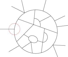
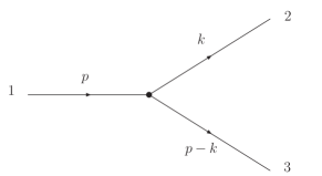
Figure 1: Light-cone supergraphs

We consider an external leg, e.g. the one marked with a dotted circle in the figure, and analyze the internal loop it connects to. The corresponding integral can be rendered finite using integrations by parts in superspace to move chiral derivatives from the internal lines onto the external one. This brings factors of momentum out of the loop integral and improves its convergence . External lines connected to a quartic vertex can be analyzed in a similar fashion. Once the first loop connected to the selected external leg is rendered finite, we move to an adjacent loop and use similar manipulations to reduce its degree of divergence to a negative value. The procedure continues until all the loops in the supergraph have been dealt with.

In order to give the reader a flavor of the kind of manipulations involved, we analyze explicitly the contribution of specific Wick contractions to the loop attached to the vertex highlighted in the graph on the left of figure 1. We isolate the vertex, which is depicted on the right hand side of the figure with the associated momenta. In position space we consider

$$\langle\Phi(z_{1})\Phi(z_{2})\Phi(z_{3})\int\!{\rm d}^{12}z\>i{\cal L}_{3}(z)\rangle\,,$$ (28)

where

$$i\,{\cal L}_{3}\,(z)=-g\,{\rm Tr}\,{\biggl{[}}\frac{1}{12}\,\frac{1}{{\partial}_{-}}\,\Phi\,[{\frac{{\bar{d}}^{4}}{{\partial}_{-}^{2}}\Phi},\partial{\frac{{\bar{d}}^{4}}{{\partial}_{-}^{2}}\Phi}]_{\star}{\biggr{]}}.$$ (29)

Among the Wick contractions contributing to (28) we consider

$${\rm Tr}\left\{\frac{1}{{\partial}_{-}}{\Delta_{2}}[\frac{{\bar{d}}^{4}}{{\partial}_{-}^{2}}\Delta_{1},\partial\,\frac{{{{\bar{d}}^{4}}}}{{\partial}_{-}^{2}}\Delta_{3}]_{\star}+\frac{1}{{\partial}_{-}}\Delta_{3}[\frac{{\bar{d}}^{4}}{{\partial}_{-}^{2}}\Delta_{1},\partial\,\frac{{{\bar{d}}^{4}}}{{\partial}_{-}^{2}}{\Delta_{2}}]_{\star}\right\}\,,$$ (30)

where the index 1 refers to the external leg while 2 and 3 identify the internal legs. In the above formula the propagators $\Delta_{n}\equiv\Delta(z-z_{n})$ are treated as matrices with indices associated with the interaction point $z$ (indices relating to $z_{n}$, $n=1,2,3$, are omitted).

The manipulations required to render a supergraph finite are exactly the same as those used in the proof of finiteness of ${\mathcal{N}}$=4 SYM in [4, 5]. An identical analysis was applied to the case of the ${\mathcal{N}}$=1 $\beta$-deformed theory in [8], where it was shown that the arguments in the ${\mathcal{N}}$=4 proof remain applicable thanks to the properties of the superspace $\star$-product . The same can be shown in the present non-supersymmetric case. In general in the presence of $\star$-products the integration by parts of chiral derivatives introduces phase factors in the superspace expressions, however, as discussed in [8], these do not affect the proof.

In order to prove that the contribution of the contractions in (30) to the loop integral is ultra-violet finite, we integrate the superspace chiral derivatives from leg $3$ to leg $2$ in the first term. Using the associativity of the $\star$-product and the cyclicity of the trace, the result can be rewritten as

$${\rm Tr}\left\{-\partial\,\frac{1}{{\partial}_{-}^{2}}\Delta_{3}[\frac{{\bar{d}}^{4}}{{\partial}_{-}^{2}}\Delta_{1},\frac{{\bar{d}}^{4}}{{\partial}_{-}}\Delta_{2}]_{\star}+\frac{1}{{\partial}_{-}}\Delta_{3}[\frac{{\bar{d}}^{4}}{{\partial}_{-}^{2}}\Delta_{1},\partial\,\frac{{\bar{d}}^{4}}{{\partial}_{-}^{2}}\Delta_{2}]_{\star}\right\}\,,$$ (31)

so that a common structure can be factored out. In momentum space we get

$$-\,{\biggl{(}}\frac{p-k}{{(p_{-}-k_{-})}^{2}}\,\frac{1}{{p_{-}}^{2}}\,\frac{1}{k_{-}}\,-\,\frac{1}{p_{-}-k_{-}}\,\frac{1}{{p_{-}}^{2}}\,\frac{k}{{k_{-}}^{2}}\,{\biggr{)}}\,{\rm Tr}\left(\Delta_{3}\,[{\bar{d}}^{4}\Delta_{1},{{\bar{d}}^{4}}{\Delta_{2}}]_{\star}\right)\,.$$ (32)

Potential ultra-violet divergences arise from loop momenta, $k$, satisfying $k\,\gg\,p$. In this limit the leading terms in parentheses cancel. This means that the logarithmically divergent contribution vanishes leaving a finite integral.

All the other Wick contractions involving both cubic and quartic vertices can be treated following similar steps. This leads to the conclusion that all the loops connected to external legs in an arbitrarily complicated supergraph have negative degree of divergence. We can then proceed to internal loops and repeat the same analysis. The ultra-violet finiteness of any supergraph then follows from the application of Weinberg’s theorem [18]. Note that the use of the theorem in the light-cone gauge is permitted due to our choice of pole structure [4], which allows for Wick rotation into Euclidean space.

*   *   *

Non-planar diagrams can be analyzed using the same methods. However, in the non-planar case the relation (27) does not hold, implying that the preliminary estimate yielding $D=0$ for all supergraphs is no longer valid. Therefore manipulations of the type outlined above are not sufficient to conclude that generic non-planar diagrams have negative superficial degree of divergence.

As already observed, it is not straightforward to deduce the finiteness of the non-supersymmetric deformation of ${\mathcal{N}}=4$ SYM considered in this paper from the ultra-violet properties of the parent ${\mathcal{N}}=4$ theory. We also point out that, while there exist other indirect arguments for the finiteness of theories obtained as deformations of ${\mathcal{N}}$=4 SYM, such as those described in [6, 20], these methods rely on supersymmetry. Hence they are not applicable to non-supersymmetric theories such as the one studied here. For these theories the light-cone analysis presented here is so far the only viable approach.

There are natural generalizations of the deformation considered in this paper. Mass terms for all the matter fields can be added preserving ultra-violet finiteness, but at the expense of scale invariance. Moreover in the light-cone superspace formulation additional parameters can be added multiplying respectively the two cubic couplings and the two quartic couplings in the action (23). This does not ruin the proof of scale invariance, since in proving the finiteness of the light-cone Green functions only cancelations among supergraphs involving separately the cubic and quartic vertices were invoked. However, this type of deformation will probably break Lorentz invariance. A more interesting generalization involves making the deformation parameters complex. A supergravity solution with 2+6 parameters, which generalizes the supergravity dual to the deformed theory considered in this paper, was obtained in [12]. We expect that the techniques used here and in [8] will allow us to prove the finiteness, in the planar approximation, of the theories deformed with complex parameters. This case is of particular interest in connection with the recent work on the role of integrability in the context of the gauge/gravity correspondence. The ${\mathcal{N}}=1$ deformation of [9] and the non-supersymmetric case studied in this paper are believed to preserve the integrability of the spectrum in the planar approximation only in the case of real deformation parameters [21, 12, 13]. Understanding whether the complex deformations indeed lead to finite theories may help to shed light on the interconnections between integrability and scale invariance.

Finally, the maximally supersymmetric ${\mathcal{N}}=8$ supergravity in four dimensions [22] has also been formulated in light-cone superspace up to second order in the gravitational coupling constant [17, 23]. The main feature of this formulation, as in the Yang–Mills case, is that it is free of both auxiliary fields and ghosts. It will be interesting to investigate whether the techniques presented in this paper and in [4, 5, 8] prove useful in the study of the ultra-violet behavior of ${\mathcal{N}}=8$ supergravity [24].

Acknowledgments

We thank Sergey Frolov and Stefan Theisen for useful discussions. SA thanks the members of the theory groups at the Harish-Chandra Research Institute and the Tata Institute of Fundamental Research for helpful comments. SA also acknowledges the kind hospitality of the Chennai Mathematical Institute. The work of SK was supported in part by a Marie Curie Intra-European Fellowship and by the EU-RTN network Constituents, Fundamental Forces and Symmetries of the Universe (MRTN-CT-2004-005104).

References

-
[1]
J. B. Kogut and K. G. Wilson, Phys. Rept.
12 (1974) 75.
K. G. Wilson, Phys. Rev. B 4 (1971) 3174.
K. G. Wilson, Phys. Rev. B 4 (1971) 3184. -
[2]
L. Brink, J. Schwarz and J. Scherk, Nucl. Phys.
B 121 (1977) 77.
F. Gliozzi, J. Scherk and D. Olive, Nucl. Phys. B 122 (1977) 256. -
[3]
L. V. Avdeev, O. V. Tarasov and A. A. Vladimirov,
Phys. Lett. B 96 (1980) 94.
M. T. Grisaru, M. Rocek and W. Siegel, Phys. Rev. Lett. 45 (1980) 1063.
M. F. Sohnius and P. C. West, Phys. Lett. B 100 (1981) 245.
W. E. Caswell and D. Zanon, Nucl. Phys. B 182 (1981) 125.
P. S. Howe, K. S. Stelle and P. K. Townsend, Nucl. Phys. B 236 (1984) 125. - [4] S. Mandelstam, Nucl. Phys. B 213 (1983) 149.
- [5] L. Brink, O. Lindgren and B. E. W. Nilsson, Phys. Lett. B 123 (1983) 323.
- [6] R. G. Leigh and M. J. Strassler, Nucl. Phys. B 447 (1995) 95 [hep-th/9503121].
-
[7]
D. Z. Freedman and U. Gursoy, JHEP 0511
(2005) 042 [hep-th/0506128].
G. C. Rossi, E. Sokatchev and Ya. S. Stanev, Nucl. Phys. B 729 (2005) 581 [hep-th/0507113].
G. C. Rossi, E. Sokatchev and Ya. S. Stanev, Nucl. Phys. B 754 (2006) 329 [hep-th/0606284].
S. Penati, A. Santambrogio and D. Zanon, JHEP 0510 (2005) 023 [hep-th/0506150].
A. Mauri, S. Penati, A. Santambrogio and D. Zanon, JHEP 0511 (2005) 024 [hep-th/0507282].
A. Mauri, S. Penati, M. Pirrone, A. Santambrogio and D. Zanon, JHEP 0608 (2006) 072 [hep-th/0605145].
V. V. Khoze, JHEP 0602 (2006) 040 [hep-th/0512194].
P. Gao and J. B. Wu, hep-th/0611128. - [8] S. Ananth, S. Kovacs and H. Shimada, JHEP 0701 (2007) 046 [hep-th/0609149].
- [9] O. Lunin and J. M. Maldacena, JHEP 0505 (2005) 033 [hep-th/0502086].
-
[10]
J. M. Maldacena, Adv. Theor. Math. Phys.
2 (1998) 231 [Int. J. Theor. Phys. 38 (1999) 1113]
[hep-th/9711200].
S. S. Gubser, I. R. Klebanov, A. M. Polyakov, Phys. Lett. B 428 (1998) 105 [hep-th/9802109].
E. Witten, Adv. Theor. Math. Phys. 2 (1998) 253 [hep-th/9802150]. - [11] N. Marcus and A. Sagnotti, Nucl. Phys. B 256 (1985) 77.
- [12] S. A. Frolov, JHEP 0505 (2005) 069 [hep-th/0503201].
- [13] S. A. Frolov, R. Roiban and A. A. Tseytlin, Nucl. Phys. B 731 (2005) 1 [hep-th/0507021].
- [14] A. Catal-Ozer, JHEP 0602 (2006) 026 [hep-th/0512290].
- [15] L. Brink, O. Lindgren and B. E. W. Nilsson, Nucl. Phys. B 212 (1983) 401.
- [16] A. K. H. Bengtsson, I. Bengtsson and L. Brink, Nucl. Phys. B 227 (1983) 41.
- [17] S. Ananth, Ph.D. Thesis, ISBN: 9780542303968 (2005).
- [18] S. Weinberg, Phys. Rev. 118 (1960) 838.
- [19] M. Grisaru, M. Rocek and W. Siegel, Nucl. Phys. B 159 (1979) 429.
-
[20]
P. C. West, Phys. Lett. B 137 (1984)
371.
A. Parkes and P. C. West, Phys. Lett. B 138 (1984) 99.
D. R. T. Jones and L. Mezincescu,Phys. Lett. B 138 (1984) 293.
S. Hamidi, J. Patera and J. H. Schwarz, Phys. Lett. B 141 (1984) 349.
S. Hamidi and J. H. Schwarz, Phys. Lett. B 147 (1984) 301.
W. Lucha and H. Neufeld, Phys. Lett. B 174 (1986) 186; Phys. Rev. D 34 (1986) 1089.
D. R. T. Jones, Nucl. Phys. B 277 (1986) 153.
A. V. Ermushev, D. I. Kazakov and O. V. Tarasov, Nucl. Phys. B 281 (1987) 72.
X. -D. Jiang and X. -J. Zhou, Phys. Rev. D 42 (1990) 2109; Phys. Lett. B 197 (1987) 156; Phys. Lett. B 216 (1989) 160.
D. I. Kazakov, Mod. Phys. Lett. A 2 (1987) 663.
O. Piguet and K. Sibold, Phys. Lett. B 177 (1986) 373; Int. J. Mod. Phys. A 1 (1986) 913.
C. Lucchesi, O. Piguet and K. Sibold, Phys. Lett. B 201 (1988) 241. - [21] D. Berenstein and S. A. Cherkis, Nucl. Phys. B 702 (2004) 49 [hep-th/0405215].
-
[22]
E. Cremmer, B. Julia and J. Scherk,
Phys. Lett. B 76 (1978) 409.
E. Cremmer and B. Julia, Phys. Lett. B 80 (1978) 48.
B. de Wit and H. Nicolai, Nucl. Phys. B 208 (1982) 323. -
[23]
A. K. H. Bengtsson, I. Bengtsson and L. Brink, Nucl. Phys. B 227 (1983) 41.
S. Ananth, L. Brink and P. Ramond, JHEP 0505 (2005) 003 [hep-th/0501079].
S. Ananth, L. Brink, R. Heise and H. G. Svendsen, Nucl. Phys. B 753 (2006) 195 [hep-th/0607019]. -
[24]
M. B. Green, J. G. Russo and P. Vanhove, [hep-th/0611273].
Z. Bern, L. J. Dixon and R. Roiban, Phys. Lett. B 644 (2007) 265 [hep-th/0611086].