(2+1)D Exotic Newton-Hooke Symmetry,
Duality and Projective Phase

Abstract

A particle system with a (2+1)D exotic Newton-Hooke symmetry is constructed by the method of nonlinear realization. It has three essentially different phases depending on the values of the two central charges. The subcritical and supercritical phases (describing 2D isotropic ordinary and exotic oscillators) are separated by the critical phase (one-mode oscillator), and are related by a duality transformation. In the flat limit, the system transforms into a free Galilean exotic particle on the noncommutative plane. The wave equations carrying projective representations of the exotic Newton-Hooke symmetry are constructed.

1 Introduction

A revival of the interest to the de Sitter (dS) and anti-de Sitter (AdS) spacetimes was provoked recently, on the one hand, by cosmological observations on accelerated expansion of our universe, and, on the other hand, by investigations on AdS/CFT correspondence. These spacetimes of constant curvature are vacuum solutions of the Einstein equations with positive and negative cosmological constants. In a limit when the velocity of light $c$ tends to infinity while cosmological constant $\Lambda$ tends to zero but keeping $c^{2}\Lambda$ finite, the symmetries of dS and AdS spacetimes become what are called the Newton-Hooke (NH) symmetries, which in a flat limit reduce to the ordinary Galilei symmetry [1, 2, 3, 4, 5, 6, 7].

In a general case of D dimensions the Galilei and NH groups admit an extension with a one central charge, while in a special case of 2+1 dimensions, they admit an exotic, two-fold central extension [8, 9, 10, 4]. The central extensions are related to a nontrivial Eilenberg-Chevalley cohomology of the corresponding Lie algebras. The exotic (2+1)D Galilei symmetry recently has attracted the attention in the context of research on non-commutative geometry and condensed matter physics [11, 12, 13, 14, 15, 16, 17, 18, 19, 20]. It is a symmetry of a free relativistic particle in a non-commutative plane, which appears from a (2+1)D theory of relativistic anyons in a special non-relativistic limit [13, 15, 16]. Surprisingly, until now, the exotic Newton-Hooke symmetry has not attracted much attention.

The present paper is devoted to investigation of classical and quantum aspects of the (2+1)D exotic Newton-Hooke (NH) symmetry. We start by constructing the exotic NH₃ algebra as a contraction of AdS₃ algebra. We then construct a particle system with the (2+1)D exotic NH symmetry by the method of nonlinear realization, and analyze its dynamics and constraint structure. We quantize the system in a reduced phase space, and show that the model has three essentially different phases depending on the values of the two central charges. The subcritical and supercritical phases describe 2D isotropic ordinary and exotic oscillators, whose spectra are characterized, respectively, by additional SO(3) rotational and SO(2,1) Lorentz symmetry. These two phases are separated by the critical phase corresponding to a one-mode oscillator, and are related by a duality transformation. We demonstrate that in the flat limit the system transforms into a free Galilean exotic particle on the noncommutative plane. For the obtained system we construct wave equations carrying projective representations of the exotic Newton-Hooke symmetry. We find the projective phase related to the nontrivial cohomology of the exotic NH symmetry, which, being associated with quasi invariance of the Lagrangian under finite NH transformations, guarantees invariance of the wave equations. We also discuss shortly some possible applications and generalizations of the exotic Newton-Hooke symmetry.

The paper is organized as follows. In Section 2, the exotic NH₃ algebra is obtained by a contraction of AdS₃. In Section 3 various forms of a classical Lagrangian for a particle with exotic NH₃ symmetry are constructed. In Sections 4, 5 and 6 we analyze classical dynamics of the system, its constraints, realization of exotic Newton-Hooke symmetry, and a manifest additional symmetry depending on the phase. In Section 7 we quantize the system in the reduced phase space. In Section 8 we discuss duality transformations. Wave equations for the system are constructed in Section 9, where we also discuss the flat limit. In Section 10 we compute the projective phase related to the nontrivial cohomology. Section 11 is devoted to the discussion and outlook. In Appendix we compute a non-trivial Eilenberg-Chevalley cohomology for the Newton-Hooke group in 2+1 dimensions.

2 Exotic NH₃ as a contraction of AdS₃

The AdS₃ algebra is given by

$$[M_{\mu\nu},M_{\lambda\sigma}]=i\left(\eta_{\mu\lambda}M_{\nu\sigma}-\eta_{\mu\sigma}M_{\nu\lambda}+\eta_{\nu\sigma}M_{\mu\lambda}-\eta_{\nu\lambda}M_{\mu\sigma}\right),$$ (2.1)

$$[M_{\mu\nu},P_{\lambda}]=i\left(\eta_{\mu\lambda}P_{\nu}-\eta_{\nu\lambda}P_{\mu}\right),$$ (2.2)

$$[P_{\mu},P_{\nu}]=-i\frac{1}{R^{2}}M_{\mu\nu},$$ (2.3)

where $\mu=0,1,2$, $\eta_{\mu\nu}=diag(-,+,+)$. If we define $M_{\mu 3}=RP_{\mu}$, the AdS₃ algebra takes a form of the $SO(2,2)$ algebra. To perform the non-relativistic contraction, rewrite (2.1)–(2.3) in the decomposed form ($\mu=0,i$; $i,j=1,2$, $\epsilon_{12}=1$),

$$[P_{0},M_{12}]=0,$$ (2.4)

$$[P_{0},M_{0i}]=iP_{i},\qquad[P_{0},P_{i}]=-i\frac{1}{R^{2}}M_{0i},$$ (2.5)

$$[M_{12},P_{i}]=i\epsilon_{ij}P_{j},\qquad[M_{12},M_{0i}]=i\epsilon_{ij}M_{0j},$$ (2.6)

$$[M_{0i},P_{j}]=-i\delta_{ij}P_{0},\qquad[M_{0i},M_{0j}]=-i\epsilon_{ij}M_{12},$$ (2.7)

$$[P_{i},P_{j}]=-i\frac{1}{R^{2}}\epsilon_{ij}M_{12},$$ (2.8)

and then replace the radius $R$ and the AdS₃ generators for the rescaled quantities,

$$P^{0}=-P_{0}\rightarrow\omega Z+\frac{1}{\omega}H,\qquad M_{0i}\rightarrow\omega K_{i},\qquad M_{12}\rightarrow\omega^{2}\tilde{Z}+J,\qquad R\rightarrow\omega R.$$ (2.9)

We introduce two new generators $Z$ and $\tilde{Z}$ that have a nature of central charges because the unextended NH₃ algebra has a non-trivial Chevalley-Eilenberg cohomology group for differential forms of degree two, see Appendix. Taking a limit $\omega\rightarrow\infty$, we get the exotic NH₃ algebra with two central charges,

$$[H,J]=0,$$ (2.10)

$$[H,K_{i}]=-iP_{i},\qquad[H,P_{i}]=i\frac{1}{R^{2}}K_{i},$$ (2.11)

$$[J,P_{i}]=i\epsilon_{ij}P_{j},\qquad[J,K_{i}]=i\epsilon_{ij}K_{j},$$ (2.12)

$$[K_{i},P_{j}]=i\delta_{ij}Z,\qquad[K_{i},K_{j}]=-i\epsilon_{ij}\tilde{Z},$$ (2.13)

$$[P_{i},P_{j}]=-i\frac{1}{{R}^{2}}\epsilon_{ij}\tilde{Z}.$$ (2.14)

This algebra was considered before in [4, 5]. In the flat limit $R\rightarrow\infty$ it transforms into algebra of exotic Galilei symmetry [8, 9, 10].

The quadratic Casimirs of NH₃ can be obtained from the two AdS₃ quadratic Casimirs

$$C_{1}=-P_{\mu}P^{\mu}+\frac{1}{2R^{2}}M_{\mu\nu}M^{\mu\nu}=P_{0}^{2}-P_{1}^{2}-P_{2}^{2}+\frac{1}{R^{2}}(J_{0}^{2}-J_{1}^{2}-J_{2}^{2}),$$ (2.15)

$$C_{2}=-P_{\mu}J^{\mu}=P_{0}J_{0}-P_{1}J_{1}-P_{2}J_{2},$$ (2.16)

corresponding to the two SO(2,2) Casimirs $M_{mn}M^{mn}$ and $\epsilon_{mnls}M^{mn}M^{ls}$, where

$$J_{\mu}=\frac{1}{2}\epsilon_{\mu\nu\lambda}M^{\nu\lambda}$$ (2.17)

with $\epsilon_{012}=+1$. Note that we should consider $C_{1}$ and $\frac{1}{R}C_{2}$ as Casimirs of the same dimension. If we perform the contraction (2.9), the finite part of the expansion gives

$${\cal C}_{1}=2\left(ZH+\frac{1}{{R}^{2}}\tilde{Z}J\right)-P_{i}^{2}-\frac{1}{{R}^{2}}K_{i}^{2},$$ (2.18)

$${\cal C}_{2}=-ZJ-\tilde{Z}H-\epsilon_{ij}P_{i}K_{j}.$$ (2.19)

It is convenient also to present the NH₃ in another, chiral basis. It’s existence is rooted in the algebra isomorphism

$$AdS_{3}\sim SO(2,2)\sim SO(2,1)\oplus SO(2,1)\sim AdS_{2}\oplus AdS_{2}.$$ (2.20)

Defining

$$J^{\pm}_{\mu}=\frac{1}{2}(J_{\mu}\mp RP_{\mu}),$$ (2.21)

we get the equivalent form of AdS₃ algebra,

$$[J^{\pm}_{\mu},J^{\pm}_{\nu}]=i\epsilon_{\mu\nu}{}^{\lambda}J^{\pm}_{\lambda},\qquad[J^{+}_{\mu},J^{-}_{\nu}]=0,$$ (2.22)

with two Casimirs

$$C^{\pm}=\eta^{\mu\nu}J^{\pm}_{\mu}J^{\pm}_{\nu}={J^{\pm}_{1}}^{2}+{J^{\pm}_{2}}^{2}-{J^{\pm}_{0}}^{2}.$$ (2.23)

Note that here $R$ is hidden in definition (2.21). In correspondence with the non-relativistic contraction realized in the non-chiral basis, we replace

$$J^{\pm}_{0}\rightarrow-\omega^{2}Z^{\pm}+{\cal J}^{\pm},\qquad J^{\pm}_{i}\rightarrow\omega{\cal J}^{\pm}_{i},$$ (2.24)

and take the limit $\omega\rightarrow\infty$. As a result we obtain the exotic NH₃ algebra in the chiral basis

$$[{\cal J}^{\pm}_{i},{\cal J}^{\pm}_{j}]=i\epsilon_{ij}Z^{\pm},\qquad[{\cal J}^{\pm},{\cal J}^{\pm}_{i}]=i\epsilon_{ij}{\cal J}^{\pm}_{j},\qquad[G^{+}_{a},G^{-}_{b}]=0,$$ (2.25)

where $G^{\pm}_{a}=Z^{\pm},{\cal J}^{\pm},{\cal J}^{\pm}_{i}$. The quadratic Casimirs are

$${\cal C}^{\pm}={{\cal J}_{i}^{\pm}}^{2}+2Z^{\pm}{\cal J}^{\pm}.$$ (2.26)

In correspondence with decomposition (2.20), we find that two-fold centrally extended NH₃ algebra is a direct sum of two centrally extended NH₂ algebras obtained by a contraction of corresponding AdS₂ chiral components. Note that usual Newton-Hooke algebra in d dimensions NH_d has only one central extension, $Z$.

The relation between generators in the chiral and non-chiral bases is

$${\cal J}^{\pm}=\frac{1}{2}\left(J\pm RH\right),\qquad{\cal J}^{\pm}_{i}=\frac{1}{2}\left(\epsilon_{ij}K_{j}\mp RP_{i}\right),\qquad Z^{\pm}=-\frac{1}{2}\left(\tilde{Z}\pm RZ\right).$$ (2.27)

3 Classical Lagrangian for a system with exotic NH₃ symmetry

To construct a Lagrangian for the exotic NH particle by the method of non-linear realization [21], we should choose a suitable coset $\frac{\cal G}{\cal H}$. In our case ${\cal G}$ is the double extended NH₃ and ${\cal H}$ is the rotation group in two dimensions. Locally we can parametrize the elements of the coset as

$$g=e^{-iHx^{0}}\;e^{iP_{i}x^{i}}\;e^{iK_{j}v^{j}}\;e^{iZc}\;e^{-i\tilde{Z}\tilde{c}}.$$ (3.1)

The (Goldstone) coordinates of the coset depend on the parameter $\tau$ that parametrizes the world line of the particle, see for example [22, 23]. The Maurer-Cartan one-form is

$$\Omega=-ig^{-1}dg=-L_{H}H+L^{i}_{P}P_{i}+L^{i}_{K}K_{i}+L_{J}J-L_{Z}Z+L_{\tilde{Z}}\tilde{Z}\,,$$ (3.2)

where

$$L_{H} = dx^{0},\qquad L^{i}_{P}=dx^{i}-v^{i}dx^{0},\qquad L^{i}_{K}=dv^{i}+\frac{x^{i}}{R^{2}}\,dx^{0},\qquad L_{J}=0,$$

$$L_{Z} = -dc-v^{i}dx^{i}+\frac{v_{i}^{2}}{2}dx^{0}+\frac{x_{i}^{2}}{2R^{2}}\,dx^{0},$$

$$L^{\tilde{Z}} = -d\tilde{c}-\frac{1}{2}\epsilon_{ij}\left(v^{i}dv^{j}+\frac{1}{R^{2}}x^{i}dx^{j}-\frac{2}{R^{2}}x^{i}v^{j}dx^{0}\right).$$ (3.3)

The one-form (3.2) satisfies the Maurer-Cartan equation $d\Omega+i\Omega\wedge\Omega=0$.

The Lagrangian is obtained as a pullback of a linear combination of nonzero one-forms invariant under rotations, $L_{H},L_{Z},L_{\tilde{Z}}$,

$${\cal L}=\mu\dot{x}^{0}+m\left(\dot{c}+v^{i}\dot{x}^{i}-\frac{v_{i}^{2}}{2}\dot{x}^{0}-\frac{x_{i}^{2}}{2R^{2}}\dot{x}^{0}\right)\\ +\kappa\left(\dot{\tilde{c}}+\frac{1}{2}\epsilon_{ij}\left(v^{i}\dot{v}^{j}+\frac{1}{R^{2}}x^{i}\dot{x}^{j}-\frac{2}{R^{2}}x^{i}v^{j}\dot{x}^{0}\right)\right),$$ (3.4)

where $\mu$ and $m$ are two parameters of dimension $R^{-1}$ while parameter $\kappa$ is dimensionless. If further fix the diffeomorphism invariance by choosing $\tau=x^{0}\equiv t$ and discard total derivative terms, we get

$${\cal L}_{nc}=m\left(v_{i}\dot{x}_{i}-\frac{v_{i}^{2}}{2}-\frac{x_{i}^{2}}{2R^{2}}\right)\\ +\frac{1}{2}\kappa\epsilon_{ij}\left(v_{i}\dot{v}_{j}+\frac{1}{R^{2}}x_{i}\dot{x}_{j}-\frac{2}{R^{2}}x_{i}v_{j}\right).$$ (3.5)

For the analysis of the dynamics and subsequent quantization of the system, it is more convenient to use another form of Lagrangian which can be obtained via a simple change of variables and parameters

$$X^{\pm}_{i} = x_{i}\pm R\epsilon_{ij}v_{j},$$ (3.6)

$$\mu_{\pm} = \frac{1}{2R^{2}}(mR\pm\kappa).$$ (3.7)

In their terms Lagrangian (3.5) rewrites

$${\cal L}_{ch}={\cal L}_{+}+{\cal L}_{-}=-\frac{1}{2}\mu_{+}\left(\epsilon_{ij}\dot{X}^{+}_{i}X^{+}_{j}+\frac{1}{R}{X^{+}_{i}}^{2}\right)-\frac{1}{2}\mu_{-}\left(-\epsilon_{ij}\dot{X}^{-}_{i}X^{-}_{j}+\frac{1}{R}{X^{-}_{i}}^{2}\right).$$ (3.8)

Coordinates $X^{\pm}_{i}$ have a sense of chiral modes of the exotic NH particle. Non-chiral, ${\cal L}_{nc}$, and chiral, ${\cal L}_{ch}$, forms of Lagrangian coincide up to a total time derivative term,

$${\cal L}_{nc}={\cal L}_{ch}+\frac{d}{dt}\Delta{\cal L},\qquad\Delta{\cal L}=\frac{m}{2}x_{i}v_{i}=\frac{m}{4R}\epsilon_{ij}X^{+}_{i}X^{-}_{j},$$ (3.9)

which has been omitted when we passed from (3.5) to (3.8), but will be important in quantum theory.

Lagrangian (3.8) can also be obtained by the method of nonlinear realization from the chiral form of exotic NH₃ algebra (2.25). In this case the elements of the coset are parametrized as

$$g=g^{+}g^{-},$$ (3.10)

with

$$g^{+} = e^{-ix^{0}R^{-1}{\cal J}^{+}}e^{-iR^{-1}X^{-}_{j}{\cal J}^{+}_{j}}e^{ic^{+}Z^{+}},$$

$$g^{-} = e^{ix^{0}R^{-1}{\cal J}^{-}}e^{iR^{-1}X^{+}_{j}{\cal J}^{-}_{j}}e^{ic^{-}Z^{-}}.$$ (3.11)

Note that there is only one time evolution variable $x^{0}$ for these chiral sectors. Difference in signs in exponents with $x^{0}$ originates from the relation $H=({\cal J}^{+}-{\cal J}^{-})/R$.

4 Classical dynamics

Variation of Lagrangian (3.5) in $v_{i}$ and $x_{i}$ gives the equations of motion

$$m(\dot{x}_{i}-v_{i})+{\kappa}\epsilon_{ij}\left(\dot{v}_{j}+R^{-2}x_{j}\right)=0,$$ (4.1)

$$m\left(\dot{v}_{i}+R^{-2}x_{i}\right)-R^{-2}\epsilon_{ij}(\dot{x}_{j}-v_{j})=0.$$ (4.2)

They can be presented in an equivalent form

$$(\dot{x}_{i}-v_{i})+\rho R\epsilon_{ij}\left(\dot{v}_{j}+R^{-2}x_{j}\right)=0,$$ (4.3)

$$(\dot{x}_{i}-v_{i})+\rho^{-1}R\epsilon_{ij}\left(\dot{v}_{j}+R^{-2}x_{j}\right)=0,$$ (4.4)

where

$$\rho=\frac{\kappa}{mR}.$$ (4.5)

For $\rho^{2}\neq 1$, the parameter transformation

$$\rho\rightarrow\rho^{-1}$$ (4.6)

provokes a mutual change of equations (4.3) and (4.4). These equations imply

$$\dot{x}_{i}-v_{i}=\dot{v}_{i}+R^{-2}x_{i}=0\qquad\to\qquad\ddot{x}_{i}+\frac{1}{R^{2}}x_{i}=0.$$ (4.7)

The system looks like a planar isotropic oscillator in both cases $\rho^{2}<1$ and $\rho^{2}>1$. We shall see that in the latter case, however, it is characterized by some exotic properties.

At critical values $\rho=\varepsilon$, $\varepsilon=\pm 1$, which separate subcritical, $\rho^{2}<1$, and supercritical, $\rho^{2}>1$, phases, Eqs. (4.3), (4.4) reduce to only one vector equation

$$(\dot{x}_{i}-v_{i})+{\varepsilon}\,R\epsilon_{ij}(\dot{v}_{j}+R^{-2}x_{j})=0.$$ (4.8)

This reflects a gauge symmetry appearing in the system in the critical phase $\rho^{2}=1$,

$$\delta_{\sigma}x_{i}=\sigma_{i}(t),\quad\delta_{\sigma}v_{i}={\varepsilon}R^{-1}\epsilon_{ij}\sigma_{j}(t).$$ (4.9)

The picture becomes more transparent if we consider the dynamics in terms of chiral coordinates (3.6). In the noncritical case transformation (4.6) assumes a change $mR\leftrightarrow\kappa$, that corresponds to a transformation

$$\mu_{\pm}\rightarrow\pm\mu_{\pm}.$$ (4.10)

Lagrangian (3.8) is invariant under transformation (4.10) accompanied with a complex coordinate transformation

$$X^{+}_{i}\rightarrow X^{+}_{i},\qquad X^{-}_{i}\rightarrow iX^{-}_{i}.$$ (4.11)

The appearance of the pure imaginary factor $i$ in transformation (4.11) is related to some peculiar properties of the supercritical phase $\rho^{2}>1$ to be discussed below. Here it is worth noting, however, that transformation (4.10), (4.11) is not a usual (discrete) symmetry of the system since it involves the change of the parameters. Moreover, transformation (4.11) itself belongs to a broad class of similarity transformations $X^{+}_{i}\rightarrow\gamma^{+}X^{+}_{i}$, $X^{-}_{i}\rightarrow\gamma^{-}X^{-}_{i}$, where $\gamma^{\pm}$ are numerical parameters, which leave invariant equations of motion but change Lagrangian. Such transformations cannot be promoted to symmetries at the quantum level, see Ref. [24] for the discussion.

For $\rho^{2}\neq 1$ equations of motion generated by Lagrangian (3.8) are

$$\dot{X}^{\pm}_{i}\pm\frac{1}{R}\epsilon_{ij}X^{\pm}_{j}=0.$$ (4.12)

The coordinates $X^{+}_{i}$ and $X^{-}_{i}$ have a sense of normal modes realizing ‘right’ and ‘left’ rotations of the same frequency $R^{-1}$,

$$X^{\pm}_{i}(t)=X^{\pm}_{i}(0)\cos R^{-1}t\mp\epsilon_{ij}X^{\pm}_{j}(0)\sin R^{-1}t.$$ (4.13)

The evolution of $x_{i}$ and $v_{i}$ is a linear superposition of these two rotations,

$$x_{i}=\frac{1}{2}(X^{+}_{i}+X^{-}_{i}),\qquad v_{i}=\frac{1}{2R}\epsilon_{ij}(X^{-}_{j}-X^{+}_{j}).$$

In the critical case $\rho=1$ ($\rho=-1$) in accordance with Eq. (3.7) we have $\mu_{-}=0$ ($\mu_{+}=0$). The chiral coordinates $X^{-}_{i}$ ($X^{+}_{i}$) disappear from Lagrangian (3.8) transforming into pure gauge variables. This corresponds to a reduction of equations (4.8) in the non-chiral basis at $\rho=\varepsilon$.

Eq. (4.12) obtained by variation of (3.8) in $X^{\pm}_{i}$, can be rewritten as $X^{\pm}_{i}\mp R\epsilon_{ij}\dot{X}^{\pm}_{j}=0$. The coordinate $X^{\pm}_{i}$ can be eliminated in terms of velocity of $X^{\pm}_{j},j\neq i$. Therefore any fixed component of the vectors $X^{+}_{i}$ and $X^{-}_{i}$ can be treated as an auxiliary variable. If we choose $i=2$ for both chiral modes, substitute

$$X^{\pm}_{2}=\mp R\dot{X}^{\pm}_{1}$$ (4.14)

into Lagrangian, and omit the total derivative term, we get an equivalent form for the Lagrangian,

$${\cal L}=\frac{1}{2}\mu_{+}R\left((\dot{X}^{+}_{1})^{2}-\frac{1}{R^{2}}X^{+2}_{1}\right)+\frac{1}{2}\mu_{-}R\left((\dot{X}^{-}_{1})^{2}-\frac{1}{R^{2}}X^{-2}_{1}\right).$$ (4.15)

This form of Lagrangian shows explicitly that the system is a sum of two harmonic oscillators of the same frequency, but it hides a 2D rotation invariance of the system.

It is worth noting that the equation $v_{i}=\dot{x}_{i}$ is generated by variation of Lagrangian (3.5) in some linear combination of $v_{i}$ and $x_{i}$, but not in $v_{i}$ itself. If we try to substitute this equation into (3.5), as a consequence we get a higher derivative Lagrangian for $x_{i}$, which will produce equations of motion for $x_{i}$ to be not equivalent to those in (4.7) [25].

5 Constraints

5.1 Non-chiral basis

System (3.5) has two pairs of primary constraints

$$\Pi_{i} = \pi_{i}+\frac{\kappa}{2}\epsilon_{ij}v_{j}\approx 0,$$ (5.1)

$$V_{i} = p_{i}-mv_{i}+\frac{\kappa}{2R^{2}}\epsilon_{ij}x_{j}\approx 0,$$ (5.2)

where $p_{i}$ and $\pi_{i}$ are the momenta canonically conjugate to $x^{i}$ and $v^{i}$. Constraints (5.1) satisfy relations

$$\{\Pi_{i},\Pi_{j}\}=\kappa\epsilon_{ij},\qquad\{V_{i},V_{j}\}=\frac{\kappa}{R^{2}}\epsilon_{ij},\qquad\{\Pi_{i},V_{j}\}=m\delta_{ij}.$$ (5.3)

Determinant of the matrix of Poisson brackets of the constraints, $A_{ab}=\{\phi_{a},\phi_{b}\}$, $\phi_{a}=(\Pi_{i},V_{i})$, is

$$\det A=m^{4}(1-\rho^{2})^{2}.$$ (5.4)

In non-critical case the matrix is non-degenerate, and (5.1), (5.2) form the set of second class constraints. At $\rho^{2}=1$ the matrix degenerates, there are first class constraints which we will analyze separately.

Canonical Hamiltonian corresponding to non-chiral Lagrangian (3.5) is

$$H_{can}=\frac{m}{2}\left(v_{i}^{2}+\frac{1}{R^{2}}x_{i}^{2}\right)+\frac{\kappa}{R^{2}}\epsilon_{ij}x_{i}v_{j}.$$ (5.5)

Adding to it a linear combination of primary constraints and applying the Dirac algorithm, for the non-critical case we get a total Hamiltonian

$$H=p_{i}v_{i}-\frac{\pi_{i}x_{i}}{R^{2}}+\frac{m}{2}\left(\frac{x_{i}^{2}}{R^{2}}-v_{i}^{2}\right),$$ (5.6)

$$\{H,\Pi_{i}\}=V_{i},\qquad\{H,V_{i}\}=-\frac{1}{R^{2}}\Pi_{i}.$$ (5.7)

The following linear combinations of the phase space coordinates,

$${\cal P}_{i}=p_{i}-\frac{\kappa}{2R^{2}}\epsilon_{ij}x_{j},\qquad{\cal K}_{i}=mx_{i}-\pi_{i}+\frac{1}{2}\kappa\epsilon_{ij}v_{j},$$ (5.8)

have zero Poisson brackets with constraints (5.1) and (5.2). These are observable variables which satisfy relations

$$\{{\cal P}_{i},{\cal P}_{j}\}=-\frac{\kappa}{R^{2}}\epsilon_{ij},\qquad\{{\cal K}_{i},{\cal P}_{j}\}=m\delta_{ij},\qquad\{{\cal K}_{i},{\cal K}_{j}\}=-\kappa\epsilon_{ij}.$$ (5.9)

For $\kappa\neq 0$ constraints (5.1) form a subset of second class constraints. Reduction on their surface allows us to express $\pi_{i}$ in terms of $v_{i}$, and results in nontrivial Poisson-Dirac brackets

$$\{x_{i},p_{j}\}=\delta_{ij},\qquad\{v_{i},v_{j}\}=-\frac{1}{\kappa}\epsilon_{ij}.$$ (5.10)

In terms of these brackets,

$$\{V_{i},V_{j}\}=-\frac{m^{2}}{\kappa}(1-\rho^{2})\epsilon_{ij}.$$ (5.11)

In correspondence with (5.4), for $\rho^{2}\neq 1$ constraints (5.2) are second class. At $\rho^{2}=1$ they are first class, and dimension of a physical subspace is less in two in comparison with a noncritical case. For $\rho^{2}\neq 1$, subsequent reduction to the surface of second class constraints (5.2) excludes the variables $v_{i}$, and for independent reduced phase space variables $x_{i}$ and $p_{i}$ we get

$$\{x_{i},x_{j}\}=\frac{\kappa}{m^{2}}\,\frac{1}{1-\rho^{2}}\epsilon_{ij},\qquad\{x_{i},p_{j}\}=\frac{1-\frac{1}{2}\rho^{2}}{1-\rho^{2}}\delta_{ij},\qquad\{p_{i},p_{j}\}=\frac{m^{2}}{4\kappa}\,\frac{\rho^{4}}{1-\rho^{2}}\epsilon_{ij}.$$ (5.12)

Dynamics is generated by the reduced phase space Hamiltonian

$$H^{*}=\frac{1}{2m}\left(p_{i}-\frac{\kappa}{2R^{2}}\epsilon_{ij}x_{j}\right)^{2}+\frac{m}{2R^{2}}(1-\rho^{2})x_{i}^{2}$$ (5.13)

being a restriction of the total Hamiltonian (5.6), to the surface of the constraints (5.1), (5.2).

From the explicit form of Hamiltonian (5.13) it is clear that the subcritical, $\rho^{2}<1$, and supercritical, $\rho^{2}>1$, cases are essentially different: in the first case energy has a sign of a parameter $m$, while in the second case it can take both signs.

Note that the symplectic structure of the reduced phase space (5.12) has a form similar to that for the Landau problem in the noncommutative plane [12, 17]. In the flat limit $R\rightarrow\infty$, the symplectic structure and Hamiltonian (5.13) take the form of those for a free particle on the noncommutative plane, which is described by the exotic Galilean symmetry with non-commuting boosts [16].

5.2 Chiral basis

In the chiral basis, the system with Lagrangian (3.8) is described by the set of constraints

$$\chi^{+}_{i}=P^{+}_{i}+\frac{1}{2}\mu_{+}\epsilon_{ij}X^{+}_{j}\approx 0,$$ (5.14)

$$\chi^{-}_{i}=P^{-}_{i}-\frac{1}{2}\mu_{-}\epsilon_{ij}X^{-}_{j}\approx 0.$$ (5.15)

Here $P^{\pm}_{i}$ are the momenta canonically conjugate to $X^{\pm}_{i}$,

$$P^{\pm}_{i}=\frac{1}{2}\left(p^{ch}_{i}\pm\frac{1}{R}\epsilon_{ij}\pi^{ch}_{j}\right).$$ (5.16)

The momenta $p^{ch}_{i}$ and $\pi^{ch}_{i}$ canonically conjugate to $x_{i}$ and $v_{i}$ are related to the corresponding momenta for non-chiral Lagrangian (3.5) by the canonical transformation

$$p_{i}^{ch}=p_{i}-\frac{m}{2}v_{i},\qquad\pi^{ch}_{i}=\pi_{i}-\frac{m}{2}x_{i}$$ (5.17)

associated with time derivative shift (3.9).

Nonzero brackets of the constraints are

$$\{\chi^{+}_{i},\chi^{+}_{j}\} = \mu_{+}\epsilon_{ij},$$ (5.18)

$$\{\chi^{-}_{i},\chi^{-}_{j}\} = -\mu_{-}\epsilon_{ij}.$$ (5.19)

In the noncritical case $\rho^{2}\neq 1$, these are two sets of second class constraints. When $\mu_{+}=0$ ($\mu_{-}=0$), the constraints $\chi^{+}_{i}$ ($\chi^{-}_{i}$) change their nature from the second to the first class, taking a form $\chi^{+}_{i}=P^{+}_{i}\approx 0$ ($\chi^{-}_{i}=P^{-}_{i}\approx 0$). In this case the degrees of freedom corresponding to the ‘$+$’ (‘$-$’) mode are pure gauge, that reflects disappearance of the corresponding term ${\cal L}_{+}$ (${\cal L}_{-}$) from Lagrangian (3.8).

Canonical Hamiltonian corresponding to the chiral Lagrangian (3.8) is

$$H_{can}=\frac{1}{2R}\left(\mu_{+}{X^{+}_{i}}^{2}+\mu_{-}{X^{-}_{i}}^{2}\right).$$ (5.20)

Define a total Hamiltonian $H=H_{can}+u^{+}_{i}\chi^{+}_{i}+u^{-}_{i}\chi^{-}_{i}$. A requirement of conservation of constraints fixes multipliers, $u^{\pm}_{i}=\mp\frac{1}{R}\epsilon_{ij}X^{\pm}_{j}$, and gives

$$H=\frac{1}{R}\epsilon_{ij}(X^{+}_{i}P^{+}_{j}-X^{-}_{i}P^{-}_{j}).$$ (5.21)

This Hamiltonian reproduces Lagrangian equations of motion for chiral coordinates (4.12).

Independent variables (observables) commuting with constraints are

$$\lambda^{+}_{i}=P^{+}_{i}-\frac{1}{2}\mu_{+}\epsilon_{ij}X^{+}_{j},\qquad\lambda^{-}_{i}=P^{-}_{i}+\frac{1}{2}\mu_{-}\epsilon_{ij}X^{-}_{j},$$ (5.22)

$$\{\lambda^{+}_{i},\chi^{\pm}_{j}\}=\{\lambda^{-}_{i},\chi^{\pm}_{j}\}=0.$$ (5.23)

They have brackets similar to the brackets of the constraints,

$$\{\lambda^{+}_{i},\lambda^{+}_{j}\}=-\mu_{+}\epsilon_{ij},\qquad\{\lambda^{-}_{i},\lambda^{-}_{j}\}=\mu_{-}\epsilon_{ij},\qquad\{\lambda^{+}_{i},\lambda^{-}_{j}\}=0.$$ (5.24)

Reduction to the surface given by (5.14) (when $\mu_{+}\neq 0$) and/or (5.15) (when $\mu_{-}\neq 0$) results in exclusion of the momenta $P^{+}_{i}$ and/or $P^{-}_{i}$. Nontrivial Dirac brackets are

$$\{X^{+}_{i},X^{+}_{j}\} = -\frac{1}{\mu_{+}}\epsilon_{ij},$$ (5.25)

$$\{X^{-}_{i},X^{-}_{j}\} = \frac{1}{\mu_{-}}\epsilon_{ij},$$ (5.26)

and reduced phase space Hamiltonian

$$H^{*}=\frac{1}{2R}\left(\mu_{+}{X^{+}_{i}}^{2}+\mu_{-}{X^{-}_{i}}^{2}\right)$$ (5.27)

coincides with the form of canonical Hamiltonian (5.20). In correspondence with non-chiral picture, for subcritical case $\rho^{2}<1$, $\mu_{\pm}>0$ for $m>0$ and $\mu_{\pm}<0$ for $m<0$, and energy takes values of the sign of the parameter $m$. In the supercritical case $\rho^{2}>1$ the constants $\mu_{+}$ and $\mu_{-}$ have opposite signs, and energy can take values of any sign.

6 Symmetries

6.1 Classical exotic Newton-Hooke symmetry

Lagrangian (3.5) is quasi-invariant under transformations generalizing Galilean translations and boosts,

$$x_{i}^{\prime}=x_{i}+\alpha_{i}\cos R^{-1}t,\qquad v_{i}^{\prime}=v_{i}-\alpha_{i}R^{-1}\sin R^{-1}t,$$ (6.1)

$$x_{i}^{\prime}=x_{i}+\beta_{i}R\sin R^{-1}t,\qquad v_{i}^{\prime}=v_{i}+\beta_{i}\cos R^{-1}t,$$ (6.2)

and is invariant under rotations and time translations,

$$x^{\prime}_{i}=x_{i}\cos\varphi+\epsilon_{ij}x_{j}\sin\varphi,\qquad v^{\prime}_{i}=v_{i}\cos\varphi+\epsilon_{ij}v_{j}\sin\varphi,$$ (6.3)

$$t^{\prime}=t-\gamma.$$ (6.4)

Newton-Hooke translations (6.1) and boosts (6.2) are related via a time translation: the former are transformed into the latter via a shift $t\rightarrow t-\frac{\pi}{2}R$ accompanied with the change of the transformation parameters $\alpha_{i}\rightarrow R\beta_{i}$.

These symmetry transformations are generated by the vector fields

$${\cal X}_{P_{i}}=\cos R^{-1}t\frac{\partial}{\partial x_{i}}-R^{-1}\sin R^{-1}t\frac{\partial}{\partial v_{i}},\qquad{\cal X}_{K_{i}}=R\sin R^{-1}t\frac{\partial}{\partial x_{i}}+\cos R^{-1}t\frac{\partial}{\partial v_{i}},$$ (6.5)

$${\cal X}_{J}=\epsilon_{ij}\left(x_{j}\frac{\partial}{\partial x_{i}}+v_{j}\frac{\partial}{\partial v_{i}}\right),\qquad{\cal X}_{H}=-\frac{\partial}{\partial t}.$$ (6.6)

The algebra of these vector fields is

$$[{\cal X}_{H},{\cal X}_{K_{i}}]=-{\cal X}_{P_{i}},\qquad[{\cal X}_{H},{\cal X}_{P_{i}}]=+\frac{1}{R^{2}}{\cal X}_{K_{i}},\qquad[{\cal X}_{K_{i}},{\cal X}_{K_{j}}]=0,\qquad[{\cal X}_{P_{i}},{\cal X}_{P_{j}}]=0,$$ (6.7)

$$[{\cal X}_{K_{i}},{\cal X}_{P_{j}}]=0,\qquad[{\cal X}_{J},{\cal X}_{P_{i}}]=\epsilon_{ij}{\cal X}_{P_{j}},\qquad[{\cal X}_{J},{\cal X}_{K_{i}}]=\epsilon_{ij}{\cal X}_{K_{j}}.$$ (6.8)

There are no central charges in this realization, and it coincides (up to the factor $i$) with the algebra of Section 2 but without central charges.

In correspondence with Eqs. (6.1), (6.2), in chiral basis Newton-Hooke translation and boost transformations have a form

$$X^{\pm}{}^{\prime}_{i}=X^{\pm}_{i}+\alpha^{\pm}_{i}(t),$$ (6.9)

where

$$\alpha^{\pm}_{i}(t)=\Delta^{\pm}_{ij}(\alpha_{j}\pm R\epsilon_{jk}\beta_{k}),$$ (6.10)

$$\Delta^{\pm}_{ij}(t)=\delta_{ij}\cos\frac{t}{R}\mp\epsilon_{ij}\sin\frac{t}{R}.$$ (6.11)

The $\Delta^{\pm}_{ij}(t)$ are rotation matrices, $\Delta_{ij}(t)\in SO(2)$, and the $\alpha^{\pm}_{i}(t)$ defined by (6.10) satisfy equations

$$\dot{\alpha}^{\pm}_{i}(t)=\mp\frac{1}{R}\epsilon_{ij}\alpha^{\pm}_{j}(t).$$ (6.12)

In terms of variables (5.22) the generators of Newton-Hooke translations and boosts are given by

$$P_{i}=\lambda^{+}_{j}\Delta^{+}_{ji}(t)+\lambda^{-}_{j}\Delta^{-}_{ji}(t),\qquad K_{i}=R\left(\lambda^{-}_{j}\Delta^{-}_{jk}(t)-\lambda^{+}_{j}\Delta^{+}_{jk}(t)\right)\epsilon_{ki}.$$ (6.13)

Due to Eq. (5.23), the set of chiral constraints is invariant with respect to these transformations,

$$\{P_{i},\chi^{\pm}_{j}\}=\{K_{i},\chi^{\pm}_{j}\}=0.$$ (6.14)

Angular momentum generating rotation symmetry is

$$J=\epsilon_{ij}(X^{+}_{i}P^{+}_{j}+X^{-}_{i}P^{-}_{j}).$$ (6.15)

Note a similar structure which have angular momentum (6.15) and total Hamiltonian (5.21). Relations (6.14) and $\{J,\chi^{\pm}_{i}\}=\epsilon_{ij}\chi^{\pm}_{j}$, $\{H,\chi^{\pm}_{i}\}=\pm\frac{1}{R}\epsilon_{ij}\chi^{\pm}_{j}$ explicitly show the invariance of the physical subspace given by the constraints (5.14), (5.15) under the Newton-Hooke transformations.

In the reduced phase space described by variables $X^{+}_{i}$ and $X^{-}_{i}$ (when $\rho^{2}\neq 1$) with symplectic structure (5.25), (5.26), the angular momentum is

$$J=\frac{1}{2}\left(\mu_{+}{X^{+}_{i}}^{2}-\mu_{-}{X^{-}_{i}}^{2}\right),$$ (6.16)

cf. (5.20).

The integrals of motion $H$, $J$, ${P}_{i}$ and ${K}_{i}$ generate the algebra,

$$\{H,J\}=0,$$ (6.17)

$$\{H,K_{i}\}=-P_{i},\qquad\{H,P_{i}\}=\frac{1}{R^{2}}K_{i},$$ (6.18)

$$\{J,P_{i}\}=\epsilon_{ij}P_{j},\qquad\{J,K_{i}\}=\epsilon_{ij}K_{j},$$ (6.19)

$$\{K_{i},P_{j}\}=m\delta_{ij},\qquad\{K_{i},K_{j}\}=-\kappa\epsilon_{ij},$$ (6.20)

$$\{P_{i},P_{j}\}=-\frac{\kappa}{R^{2}}\epsilon_{ij}.$$ (6.21)

This is a classical analog of the exotic NH₃ algebra (2.10)–(2.14) with parameters $m$ and $\kappa$ playing the role of the central charges $Z$ and $\tilde{Z}$, respectively. Making use of the explicit form of integrals $H$, $J$, ${P}_{i}$ and ${K}_{i}$, one finds that on the constraint surface the Casimirs (2.18) and (2.19) take zero values. As a result, in the non-critical case the Hamiltonian and angular momentum are represented in terms of NH translations and boosts generators as

$$H = \frac{1}{m(1-\rho^{2})}\left(\frac{1}{2}\left(P_{i}^{2}+R^{-2}K_{i}^{2}\right)-\rho R^{-1}\epsilon_{ij}K_{i}P_{j}\right),$$ (6.22)

$$J = \frac{1}{m(1-\rho^{2})}\left(\epsilon_{ij}K_{i}P_{j}-\frac{1}{2}\rho R\left(P_{i}^{2}+R^{-2}K_{i}^{2}\right)\right).$$ (6.23)

The linear combinations of $P_{i}$ and $K_{i}$ corresponding to chiral generators (2.27) are given here in terms of variables $\lambda^{\pm}_{i}$,

$${\cal J}^{\pm}_{i}=\mp R\lambda^{\pm}_{j}\Delta^{\pm}_{ji}(t).$$ (6.24)

The equations

$$\frac{\partial{\cal J}^{\pm}_{i}}{\partial t}=\pm\frac{1}{R}\epsilon_{ij}{\cal J}^{\pm}_{j}$$ (6.25)

guarantee that they are integrals of motion, $\frac{d}{dt}{\cal J}^{\pm}_{i}=\frac{\partial{\cal J}^{\pm}_{i}}{\partial t}+\{{\cal J}^{\pm}_{i},H\}=0$. Note also that on the constraint surface (5.14), (5.15) these integrals can be presented in the form

$${\cal J}^{\pm}_{i}=R\mu_{\pm}\epsilon_{ij}X_{j}^{\pm}(0).$$ (6.26)

Together with ${\cal J}^{\pm}=\frac{1}{2}(J\pm RH)$, where $H$ corresponds to the total Hamiltonian, integrals (6.26) generate classical analog of the exotic NH₃ algebra (2.25) in the chiral form, in which

$$Z^{+}=-R^{2}\mu_{+},\qquad Z^{-}=R^{2}\mu_{-}.$$ (6.27)

In the critical case corresponding to $\rho=1$ ($\mu_{-}=0$) or $\rho=-1$ ($\mu_{+}=0$), the symmetry of the system is reduced to the centrally extended NH₂ algebra generated by ${\cal J}^{+}$, ${\cal J}^{+}_{i}$ and $Z^{+}$, or by ${\cal J}^{-}$, ${\cal J}^{-}_{i}$ and $Z^{-}$. Here the Hamiltonian and angular momentum on the one hand, and translations and boosts generators on the other hand are linearly dependent,

$$\mu_{-}=0 : \quad H=R^{-1}J=\frac{1}{2m}P_{i}^{2},\qquad P_{i}=-R^{-1}\epsilon_{ij}K_{j},$$ (6.28)

$$\mu_{+}=0 : \quad H=-R^{-1}J=\frac{1}{2m}P_{i}^{2},\qquad P_{i}=R^{-1}\epsilon_{ij}K_{j}.$$ (6.29)

Note that the sign of $H$ is defined by the sign of the mass parameter $m$.

In the non-chiral basis the generators of Newton-Hooke translations and boosts are given in terms of observable variables (5.8),

$$P_{i}={\cal P}_{i}\cos\frac{t}{R}+\frac{1}{R}{\cal K}_{i}\sin\frac{t}{R},\qquad K_{i}={\cal K}_{i}\cos\frac{t}{R}-R{\cal P}_{i}\sin\frac{t}{R},$$ (6.30)

while the angular momentum is

$$J=\epsilon_{ij}(x_{i}p_{j}+v_{i}\pi_{j}).$$ (6.31)

Together with total Hamiltonian (5.6) they generate classical algebra (6.17)–(6.21).

In the reduced phase space with coordinates $x_{i},$ $p_{i}$, integrals $P_{i}$, $K_{i}$ and $J$ take the form

$$P_{i}={\cal P}_{i}\cos\frac{t}{R}+\frac{1}{R}\tilde{\cal K}_{i}\sin\frac{t}{R},\qquad K_{i}=\tilde{\cal K}_{i}\cos\frac{t}{R}-R{\cal P}_{i}\sin\frac{t}{R},$$ (6.32)

$$J=\frac{m^{2}}{2\kappa}\left(\left(x_{i}+\frac{\kappa}{m^{2}}\epsilon_{ij}p_{j}\right)^{2}-(1-\rho^{2})x_{i}^{2}\right),$$ (6.33)

where

$$\tilde{\cal K}_{i}=mx_{i}\left(1-\frac{1}{2}\rho^{2}\right)+\frac{\kappa}{m}\epsilon_{ij}p_{j}.$$ (6.34)

Together with Hamiltonian (5.13) they satisfy the same classical algebra (6.17)–(6.21) with respect to the reduced symplectic structure (5.12).

6.2 SO(3) and SO(2,1) symmetry

Let us now show that our system has an additional symmetry. For the chiral Lagrangian this additional symmetry is manifest, its explicit form depends of the phase we consider.

Define the dimensionless (rescaled) coordinates

$$\sqrt{|\mu^{+}|}X^{+}_{1}=Y_{1},\quad\sqrt{|\mu^{+}|}X^{+}_{2}=Y_{2},\quad\sqrt{|\mu^{-}|}X^{-}_{1}=Y_{3},\quad\sqrt{|\mu^{-}|}X^{-}_{2}=Y_{4}.$$ (6.35)

In terms of these coordinates the chiral Lagrangian is written as

$${\cal L}_{ch}=-\frac{1}{2}\left(\dot{Y}^{T}\Omega Y+\frac{1}{R}{Y}^{T}\eta Y\right)=-\frac{1}{2}\left(\dot{Y}^{A}\Omega_{AB}Y^{B}+\frac{1}{R}{Y}^{A}\eta_{AB}Y^{B}\right),$$ (6.36)

where

$$\eta_{AB}=\left(\begin{array}[]{cccc}\varepsilon_{+}&.&.&.\\ .&\varepsilon_{+}&.&.\\ .&.&\varepsilon_{-}&.\\ .&.&.&\varepsilon_{-}\\ \end{array}\right),\qquad\Omega_{AB}=\left(\begin{array}[]{cccc}.&\varepsilon_{+}&.&.\\ -\varepsilon_{+}&.&.&.\\ .&.&.&-\varepsilon_{-}\\ .&.&\varepsilon_{-}&.\\ \end{array}\right),$$ (6.37)

$\varepsilon_{\pm}$ are the signs of $\mu_{\pm}$, and the matrices $\eta$ and $\Omega$ satisfy the relations $\eta^{2}=1,$ $\Omega^{T}=-\Omega,$ $\Omega\Omega=-1$. The potential term is invariant under transformations $Y\rightarrow OY$, $O^{T}\eta O=\eta$, which are the SO(4) rotations in the subcritical case with $\varepsilon_{+}\varepsilon_{-}=+1$, and are the pseudo-rotations SO(2,2)$\sim$AdS₃ in supercritical sector characterized by the relation $\varepsilon_{+}\varepsilon_{-}=-1$. On the other hand, the first, kinetic term is invariant under the Sp(4) transformations with symplectic metric $\Omega$, $Y\rightarrow CY$, $C^{T}\Omega C=\Omega$. The symmetry of Lagrangian corresponds to the intersection of SO(4) (or, SO(2,2)) and Sp(4). Considering an infinitesimal transformation $\delta Y=\omega Y$, we find that the constant matrix $\omega$ has to satisfy equations $\omega^{T}\eta+\eta\omega=0$, $\omega^{T}\Omega+\Omega\omega=0$. A simple analysis of these equations with subsequent application of the Noether theorem results finally in the set of the four integrals of motion which are $H$, $J$ and

$$I_{1}=\frac{1}{2}\varepsilon_{+}\sqrt{\left|\frac{\mu_{-}}{\mu_{+}}\right|}\left(P_{2}^{+}X_{2}^{-}-P_{1}^{+}X_{1}^{-}\right)+\frac{1}{2}\varepsilon_{-}\sqrt{\left|\frac{\mu_{+}}{\mu_{-}}\right|}\left(X_{1}^{+}P_{1}^{-}-X_{2}^{+}P_{2}^{-}\right),$$ (6.38)

$$I_{2}=-\frac{1}{2}\varepsilon_{+}\sqrt{\left|\frac{\mu_{-}}{\mu_{+}}\right|}\left(P_{2}^{+}X_{1}^{-}+P_{1}^{+}X_{2}^{-}\right)+\frac{1}{2}\varepsilon_{-}\sqrt{\left|\frac{\mu_{+}}{\mu_{-}}\right|}\left(X_{1}^{+}P_{2}^{-}+X_{2}^{+}P_{1}^{-}\right).$$ (6.39)

On the surface of the constraints (5.14), (5.15) these two new integrals take a form

$$I_{1}=\frac{1}{2}\sqrt{|\mu_{+}\mu_{-}|}\,(X^{+}_{1}X^{-}_{2}+X^{+}_{2}X^{-}_{1}),\qquad I_{2}=\frac{1}{2}\sqrt{|\mu_{+}\mu_{-}|}\,(X^{+}_{2}X^{-}_{2}-X^{+}_{1}X^{-}_{1}).$$ (6.40)

In subcritical case integral $I_{1}$ generates 2D rotations in the planes $(Y_{1},Y_{3})$ and $(Y_{2},Y_{4})$, while $I_{2}$ generates rotations in the planes $(Y_{1},Y_{4})$ and $(Y_{2},Y_{3})$. In supercritical case the 2D rotations are changed for 2D Lorentz transformations in the same planes. Being time-independent, these integrals commute with the Hamiltonian, $\{H,I_{1}\}=\{H,I_{2}\}=0$, and together with rescaled angular momentum

$$I_{3}=\frac{1}{2}J$$ (6.41)

they generate the Lie algebra

$$\{I_{1},I_{2}\}=\varepsilon_{+}\varepsilon_{-}I_{3},\qquad\{I_{3},I_{1}\}=I_{2},\qquad\{I_{2},I_{3}\}=I_{1}.$$ (6.42)

In subcritical case (6.42) is identified as a classical rotation symmetry algebra $so(3)$, while in supercritical case it is a Lorentz algebra $so(2,1)$. Note also that the brackets of the integrals $I_{1,2}$ with the Newton-Hooke translation and boost generators are reduced to some linear combinations of the latter.

7 Reduced phase space quantization

In correspondence with classical relations (5.25), (5.26), in subcritical case $\rho^{2}<1$ with $\mu_{+}>0$, $\mu_{-}>0$, one defines two sets of creation-annihilation oscillator operators

$$a_{+}=\sqrt{\frac{|\mu_{+}|}{2}}\,(X^{+}_{2}+iX^{+}_{1}),\qquad a_{-}=\sqrt{\frac{|\mu_{-}|}{2}}\,(X^{-}_{1}+iX^{-}_{2}),\qquad a_{\pm}^{\dagger}=\left(a_{\pm}\right)^{\dagger},$$ (7.1)

$$[a_{+},a^{\dagger}_{+}]=1,\qquad[a_{-},a^{\dagger}_{-}]=1,\qquad[a_{+},a_{-}]=[a_{+},a^{\dagger}_{-}]=0.$$ (7.2)

We put here parameters $\mu_{\pm}$ under the modulus sign having in mind further generalization. Let us construct Hamiltonian and angular momentum operators fixing the symmetrized ordering in (5.27) and (6.16). We get

$$H=R^{-1}\left(a^{\dagger}_{+}a_{+}+a^{\dagger}_{-}a_{-}+1\right),\qquad J=a^{\dagger}_{+}a_{+}-a^{\dagger}_{-}a_{-}\,.$$ (7.3)

Quantum system is an ordinary planar isotropic oscillator of frequency $R^{-1}$. Quantum Newton-Hooke chiral operators ${\cal J}_{i}^{\pm}$ are constructed via (6.26), (7.1) and relations inverse to (4.13),

$$\mathcal{J}_{1}^{+}=R\sqrt{\frac{\mu_{+}}{2}}\left(e^{-itR^{-1}}a^{\dagger}_{+}+e^{itR^{-1}}a_{+}\right),\quad\mathcal{J}_{2}^{+}=-iR\sqrt{\frac{\mu_{+}}{2}}\left(e^{-itR^{-1}}a^{\dagger}_{+}-e^{itR^{-1}}a_{+}\right),$$ (7.4)

$$\mathcal{J}_{1}^{-}=iR\sqrt{\frac{\mu_{-}}{2}}\left(e^{-itR^{-1}}a^{\dagger}_{-}-e^{itR^{-1}}a_{-}\right),\quad\mathcal{J}_{2}^{-}=-R\sqrt{\frac{\mu_{-}}{2}}\left(e^{-itR^{-1}}a^{\dagger}_{-}+e^{itR^{-1}}a_{-}\right).$$ (7.5)

They form the exotic NH₃ algebra from Section 2. Energy takes positive values, $E_{n_{+},n_{-}}=R^{-1}(n_{+}+n_{-}+1)$, while angular momentum can take values of both signs, $j_{n_{+},n_{-}}=n_{+}-n_{-}$, where $n_{\pm}=0,1,\ldots$ are the eigenvalues of the number operators $N_{\pm}=a_{\pm}^{\dagger}a_{\pm}$, $N_{\pm}|n_{+},n_{-}\rangle=n_{\pm}|n_{+},n_{-}\rangle$.

In subcritical phase $\rho^{2}<1$ with $\mu_{+}<0$, $\mu_{-}<0$, the operators $a_{+}$ and $a_{-}$ are realized as in (7.1) with the substitution $X^{+}_{1}\leftrightarrow X^{+}_{2}$, $X^{-}_{1}\leftrightarrow X^{-}_{2}$. This provokes the change of global signs in Hamiltonian and angular momentum,

$$H=-R^{-1}\left(a^{\dagger}_{+}a_{+}+a^{\dagger}_{-}a_{-}+1\right),\qquad J=-a^{\dagger}_{+}a_{+}+a^{\dagger}_{-}a_{-}\,.$$ (7.6)

In the supercritical case $\rho>1$ ($\mu_{+}>0$, $\mu_{-}<0$), operator $a_{+}$ is defined as in (7.1) while $a_{-}$ is obtained via the substitution $X^{-}_{1}\leftrightarrow X^{-}_{2}$. Here

$$H=R^{-1}\left(a^{\dagger}_{+}a_{+}-a^{\dagger}_{-}a_{-}\right),\qquad J=a^{\dagger}_{+}a_{+}+a^{\dagger}_{-}a_{-}+1.$$ (7.7)

This is an exotic oscillator with interchanged Hamiltonian and angular momentum. Energy can take positive and negative values, $E_{n_{+},n_{-}}=R^{-1}(n_{+}-n_{-})$, $n_{\pm}=0,1,\ldots$, and is not restricted from below. Angular momentum can take only positive values, $j_{n_{+},n_{-}}=n_{+}+n_{-}+1$, i.e. the both modes are ‘right’.

In the supercritical case $\rho<-1$ ($\mu_{+}<0$, $\mu_{-}>0$), the role of the modes is changed: the energy for the mode $X^{+}$ is negative, while for $X^{-}$ is positive. In this case $a_{-}$ is defined as in (7.1), while $a_{+}$ is realized via the change $X^{+}_{1}\leftrightarrow X^{+}_{2}$. As a result,

$$H=R^{-1}\left(-a^{\dagger}_{+}a_{+}+a^{\dagger}_{-}a_{-}\right),\qquad J=-\left(a^{\dagger}_{+}a_{+}+a^{\dagger}_{-}a_{-}+1\right).$$ (7.8)

We have, again, an exotic oscillator, but now with both modes to be ‘left’.

The expressions for Hamiltonian and angular momentum for all four cases can be unified as

$$H=R^{-1}\left(\varepsilon_{+}a^{\dagger}_{+}a_{+}+\varepsilon_{-}a^{\dagger}_{-}a_{-}+\frac{1}{2}(\varepsilon_{+}+\varepsilon_{-})\right),\qquad J=\varepsilon_{+}a^{\dagger}_{+}a_{+}-\varepsilon_{-}a^{\dagger}_{-}a_{-}+\frac{1}{2}(\varepsilon_{+}-\varepsilon_{-}),$$ (7.9)

where $\varepsilon_{\pm}=\mathrm{sign}\,\mu_{\pm}$.

The boost and translation generators are given in terms of the chiral integrals,

$$K_{i}=-\epsilon_{ij}\left(\mathcal{J}_{j}^{+}+\mathcal{J}_{j}^{-}\right),\qquad P_{i}=-\frac{1}{R}\left(\mathcal{J}_{i}^{+}-\mathcal{J}_{i}^{-}\right),$$ (7.10)

which can be presented in a compact form generalizing (7.4), (7.5) for the case of arbitrary signs of $\mu_{\pm}$,

$$\mathcal{J}_{j}^{+}=\left(-i\right)^{j-1}\left(\varepsilon_{+}\right)^{j+1/2}R\sqrt{\frac{|\mu_{+}|}{2}}\left(e^{-i\varepsilon_{+}tR^{-1}}a^{\dagger}_{+}-\left(-1\right)^{j}\varepsilon_{+}e^{i\varepsilon_{+}tR^{-1}}a_{+}\right),$$ (7.11)

$$\mathcal{J}_{j}^{-}=\left(i\right)^{j}\left(\varepsilon_{-}\right)^{j-1/2}R\sqrt{\frac{|\mu_{-}|}{2}}\left(e^{-i\varepsilon_{-}tR^{-1}}a^{\dagger}_{-}+\left(-1\right)^{j}\varepsilon_{-}e^{i\varepsilon_{-}tR^{-1}}a_{-}\right),$$ (7.12)

where we imply $(-1)^{1/2}=i$.

The ladder operators $I_{+}=I_{1}+iI_{2}$ and $I_{-}=I_{+}^{\dagger}$ of the additional SO(3) ($\varepsilon_{+}\varepsilon_{-}=+1$), or SO(2,1) ($\varepsilon_{+}\varepsilon_{-}=-1$) symmetry,

$$[I_{+},I_{-}]=\varepsilon_{+}\varepsilon_{-}iI_{3},\qquad[I_{3},I_{\pm}]=\pm iI_{\pm},$$ (7.13)

corresponding to complex combinations of the classical integrals (6.40) are given by

$$\varepsilon_{+}\varepsilon_{-}=+1:\qquad I_{1}+i\varepsilon_{+}I_{2}=a^{\dagger}_{+}a_{-},$$ (7.14)

$$\varepsilon_{+}\varepsilon_{-}=-1:\qquad I_{1}+i\varepsilon_{+}I_{2}=ia^{\dagger}_{+}a_{-}^{\dagger}.$$ (7.15)

In the critical phase with $\mu_{-}=0$ we have a one-mode oscillator with $\quad E_{n_{+}}=\varepsilon_{+}R^{-1}\left(n_{+}+\frac{1}{2}\right),$ $j_{n_{+}}=\varepsilon_{+}\left(n_{+}+\frac{1}{2}\right)$, while for $\mu_{+}=0$ we have $E_{n_{-}}=\varepsilon_{-}R^{-1}\left(n_{-}+\frac{1}{2}\right),$ $j_{n_{-}}=-\varepsilon_{-}\left(n_{-}+\frac{1}{2}\right)$. The generators of the corresponding centrally extended NH₂ symmetry are given, respectively, by Eq. (7.11) or (7.12), and by Eq. (7.9) if we put in the latter the parameter $\varepsilon_{-}$ or $\varepsilon_{+}$ equal to zero.

8 Duality

Let us clarify the relation between the sub- and super-critical phases in the light of duality transformation, which can be presented in three equivalent ways,

$$\rho\rightarrow\rho^{-1};\qquad mR\leftrightarrow\kappa;\qquad\mu_{\pm}\rightarrow\pm\mu_{\pm}.$$ (8.1)

The duality induces a mutual transformation between the sub- and super-critical phases, and between two critical phases given by $\mu_{+}=0$, $\mu_{-}<0$ and $\mu_{+}=0$, $\mu_{-}>0$, while it leaves invariant the critical phases with $\mu_{-}=0$, see Figure 1.

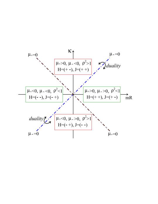
Figure 1: Phases and duality.

In accordance with Eqs. (7.9)–(7.12), duality transformation (8.1) induces the transformations

$$J\leftrightarrow RH,$$ (8.2)

$$P_{i} \rightarrow P_{i}^{\prime}=\frac{1}{2}\left((P_{1}+P_{2})+(-1)^{i}R^{-1}(K_{1}+K_{2})\right),$$ (8.3)

$$K_{i} \rightarrow K_{i}^{\prime}=\frac{1}{2}\left((-1)^{i+1}(K_{1}-K_{2})+R(P_{2}-P_{1})\right).$$ (8.4)

In terms of chiral integrals (2.27), these transformations are equivalent to

$${\cal J}^{\pm}\rightarrow\pm{\cal J}^{\pm},\qquad{\cal J}^{+}_{i}\rightarrow{\cal J}^{+}_{i},\qquad{\cal J}^{-}_{1}\rightarrow{\cal J}_{2}^{-},\qquad{\cal J}^{-}_{2}\rightarrow{\cal J}_{1}^{-}.$$ (8.5)

Having in mind also (6.27), we have

$$Z^{\pm}\rightarrow\pm Z^{\pm}.$$ (8.6)

Using relations (8.5), (8.6), we conclude that the duality does not change the algebra (2.25) of integrals of motion, and so, it is an automorphism of the exotic Newton-Hooke algebra.

On the other hand, the sub- and super-critical phases are essentially different from the viewpoint of the structure of the energy and angular momentum levels. In correspondence with (7.9), the energy levels and angular momentum values are

$$E_{n_{+},n_{-}}=\frac{1}{R}\left(\varepsilon_{+}n_{+}+\varepsilon_{-}n_{-}+\frac{1}{2}(\varepsilon_{+}+\varepsilon_{-})\right),\qquad j_{n_{+},n_{-}}=\varepsilon_{+}n_{+}-\varepsilon_{-}n_{-}+\frac{1}{2}(\varepsilon_{+}-\varepsilon_{-}),$$ (8.7)

where $n_{\pm}=0,1,\ldots$. Every such a level in subcritical case $\varepsilon_{+}\varepsilon_{-}=+1$ has a finite degeneration equal to $2j_{{}_{<}}+1$, where

$$j_{{}_{<}}=\frac{1}{2}\left(n_{+}+n_{-}\right),$$ (8.8)

and corresponding energy eigenstates are characterized by the quantum numbers $n_{+}$ and $n_{-}$ laying on the straight lines restricted by vertical and horizontal axes, see Figure 2. The $so(3)$ ladder operators given by Eq. (7.14) act along these lines. On the line with $n_{+}+n_{-}=2j_{{}_{<}}$, the $so(3)$ Casimir operator $C_{so(3)}=I_{1}^{2}+I_{2}^{2}+I_{3}^{2}$ takes a value $j_{{}_{<}}(j_{{}_{<}}+1)$.

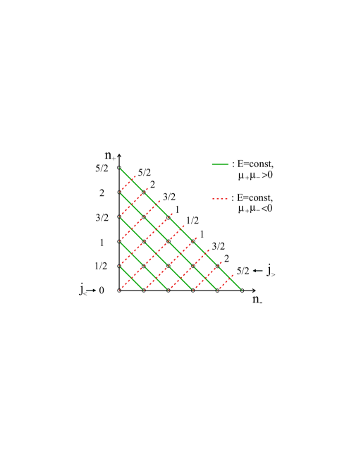
Figure 2: Constant energy levels.

In supercritical phase $\varepsilon_{+}\varepsilon_{-}=-1$, and constant energy levels correspond to the dotted straight lines $n_{+}-n_{-}=const$ on Figure 2. The $so(2,1)$ ladder operators (7.15) act along them. Every energy level is infinitely degenerated, and the $so(2,1)$ Casimir operator $C_{so(2,1)}=I_{1}^{2}+I_{2}^{2}-I_{3}^{2}$ takes a value $-j_{{}_{>}}(j_{{}_{>}}-1)$, where

$$j_{{}_{>}}=\frac{1}{2}\left(|n_{+}-n_{-}|+1\right).$$ (8.9)

Every such a straight line corresponds to the infinite-dimensional half-bounded unitary representation of $so(2,1)$ algebra, on which the $so(2,1)$ compact generator $I_{3}$ takes the values $i_{3}=\varepsilon_{+}\frac{1}{2}(n_{+}+n_{-}+1)$. This can be presented equivalently as $i_{3}=\varepsilon_{+}(j_{{}_{>}}+k),$ where $k=n_{-}=0,1,\ldots$ for $n_{+}\geq n_{-}$, and $k=n_{+}=0,1,\ldots$ for $n_{-}\geq n_{+}$ . Therefore, we have here the so called discrete series of representations $D^{+}_{j_{{}_{>}}}$ (for $\varepsilon_{+}=+1$) and $D^{-}_{j_{{}_{>}}}$ (for $\varepsilon_{+}=-1$) of $SL(2,R)$ in terminology of Bargmann [26].

We conclude that the duality transformation (8.1) provokes a mutual change of compact, $so(3)$, and noncompact, $so(2,1)$, symmetries in accordance with Eq. (7.13). This is accompanied by a radical change of the energy degeneration from the finite to the infinite, or inversely.

9 Wave equations

Here we shall quantize the system using the method of Gupta-Bleuler, that will allow us to construct the set of wave equations realizing the exotic Newton-Hooke symmetry. Using them, in the next Section we shall identify corresponding projective phases associated with Newton-Hooke translations and boosts transformations.

9.1 Chiral basis

Let us choose two complex linear combinations of the constraints (5.14), (5.15) such that

• they would commute between themselves,

• at the quantum level they would have a nature of annihilation operators having nontrivial kernels,

• their set would be consistent with dynamics, i.e. their commutators with Hamiltonian would be proportional to the chosen combinations of the constraints.

Then at the quantum level these linear combinations will separate a physical subspace of the system.

In correspondence with the structure of the brackets of the chiral constraints (5.14), (5.15), for $\rho^{2}\neq 1$ it is necessary to distinguish four cases in dependence on the signs of $\mu_{\pm}$. For $\mu_{+}>0$, $\mu_{-}>0$, the suitable choice of the linear combinations of the constraints is

$$\chi^{+}_{1}+i\chi^{+}_{2}\approx 0,\qquad\chi^{-}_{1}-i\chi^{-}_{2}\approx 0.$$ (9.1)

In coordinate representation they transform into quantum equations

$$\left(\partial_{\bar{\cal Z}^{+}}+\frac{\mu_{+}}{4}{\cal Z}^{+}\right)\Psi=0,\qquad\left(\partial_{{\cal Z}^{-}}+\frac{\mu_{-}}{4}\bar{\cal Z}^{-}\right)\Psi=0,$$ (9.2)

where $\partial_{\bar{\cal Z}^{+}}=\partial/\partial\bar{\cal Z}^{+}$, $\partial_{{\cal Z}^{-}}=\partial/\partial{\cal Z}^{-}$, and we have introduced two independent complex chiral variables

$${\cal Z}^{+}=X^{+}_{1}+iX^{+}_{2},\qquad{\cal Z}^{-}=X^{-}_{1}+iX^{-}_{2}.$$ (9.3)

The dynamics is given by the Schrödinger equation

$$\left(i\partial_{t}-\frac{1}{R}\left({\cal Z}^{+}\partial_{{\cal Z}^{+}}-\bar{\cal Z}^{+}\partial_{\bar{\cal Z}^{+}}-{\cal Z}^{-}\partial_{{\cal Z}^{-}}+\bar{\cal Z}^{-}\partial_{\bar{\cal Z}^{-}}\right)\right)\Psi=0,$$ (9.4)

where the linear differential operator in complex chiral variables is a quantum analog of the total chiral Hamiltonian (5.21). Eqs. (9.2) and (9.4) represent the set of wave equations for our particle system with exotic Newton-Hooke symmetry.

The solution of the quantum equations (9.2) is

$$\Psi_{phys}=\exp\left(-\frac{\mu_{+}}{4}|{\cal Z}^{+}|^{2}-\frac{\mu_{-}}{4}|{\cal Z}^{-}|^{2}\right)\psi({\cal Z}^{+},\bar{\cal Z}^{-}).$$ (9.5)

The action of the Hamiltonian and angular momentum operators on the states (9.5) is reduced to

$$H\Psi_{phys}=\exp(.)\frac{1}{R}\left({\cal Z}^{+}\partial_{{\cal Z}^{+}}+\bar{\cal Z}^{-}\partial_{\bar{\cal Z}^{-}}\right)\psi({\cal Z}^{+},\bar{\cal Z}^{-}),$$ (9.6)

$$J\Psi_{phys}=\exp(.)\frac{1}{R}\left({\cal Z}^{+}\partial_{{\cal Z}^{+}}-\bar{\cal Z}^{-}\partial_{\bar{\cal Z}^{-}}\right)\psi({\cal Z}^{+},\bar{\cal Z}^{-}).$$ (9.7)

The energy and angular momentum eigenfunctions are given by the states (9.5) with monomial wave functions $\psi({\cal Z}^{+},\bar{\cal Z}^{-})$,

$$\psi_{n_{+},n_{-}}({\cal Z}^{+},\bar{\cal Z}^{-})=\frac{1}{\sqrt{n_{+}!n_{-}!}}\left(\sqrt{\frac{\mu_{+}}{2}}{\cal Z}^{+}\right)^{n_{+}}\left(\sqrt{\frac{\mu_{-}}{2}}\bar{\cal Z}^{-}\right)^{n_{-}},\qquad n_{+},n_{-}=0,1,\ldots,$$ (9.8)

which correspond to the energy and angular momentum eigenvalues $E_{n_{+},n_{-}}=\frac{1}{R}(n_{+}+n_{-})$, $j_{n_{+},n_{-}}=n_{+}-n_{-}$. Note that a simple quantum shift in energy [equal to $-\frac{1}{R}\hbar$, $\hbar=1$] in comparison with the reduced phase space quantization scheme is related to our choice of the normal quantum ordering: here we take a Hamiltonian operator corresponding to the classical expression (5.21).

These results are in a complete correspondence with reduced phase space quantization scheme [up to inessential shift in energy], and what we get here is the holomorphic representation for the 2D oscillator system.

The quantization scheme is generalized directly for other three cases of the signs $\varepsilon_{+}$ and $\varepsilon_{-}$ of the parameters $\mu_{+}$ and $\mu_{-}$. The wave equations separating physical states are given by the linear combinations of the constraints $\chi^{+}_{i}$ and $\chi^{-}_{i}$,

$$\left(\chi^{+}_{1}+i\varepsilon_{+}\chi^{+}_{2}\right)\Psi=0,\qquad\left(\chi^{-}_{1}-i\varepsilon_{-}\chi^{-}_{2}\right)\Psi=0.$$ (9.9)

In the table we summarize all the cases.

Phase	$\varepsilon_{+},$ $\varepsilon_{-}$	$m,$ $\kappa$	Constraints	$\psi(.,.)$
$\rho^{2}<1$	$+1,+1$	$m>0,$ $|\kappa|<mR$	$\chi^{+}_{1}+i\chi^{+}_{2},$ $\chi^{-}_{1}-i\chi^{-}_{2}$	$\overset{}{\psi({\cal Z}^{+},\bar{\cal Z}^{-})}$
$\rho^{2}<1$	$-1,-1$	$m<0$, $|\kappa|<mR$	$\chi^{+}_{1}-i\chi^{+}_{2},$ $\chi^{-}_{1}+i\chi^{-}_{2}$	$\psi(\bar{\cal Z}^{+},{\cal Z}^{-})$
$\rho^{2}>1$	$+1,-1$	$-\infty<m<\infty$, $\kappa>|m|R$	$\chi^{+}_{1}+i\chi^{+}_{2},$ $\chi^{-}_{1}+i\chi^{-}_{2}$	$\psi({\cal Z}^{+},{\cal Z}^{-})$
$\rho^{2}>1$	$-1,+1$	$-\infty<m<\infty$, $\kappa<|m|R$	$\chi^{+}_{1}-i\chi^{+}_{2},$ $\chi^{-}_{1}-i\chi^{-}_{2}$	$\psi(\bar{\cal Z}^{+},\bar{\cal Z}^{-})$

Corresponding solutions describing physical states have a form similar to (9.5),

$$\Psi_{phys}=\exp\left(-\frac{|\mu_{+}|}{4}|{\cal Z}^{+}|^{2}-\frac{|\mu_{-}|}{4}|{\cal Z}^{-}|^{2}\right)\psi(.,.),$$ (9.10)

with the arguments of the function $\psi$ specified in the table. The action of $H$ and $J$ on these states has a form similar to (9.6), (9.7): they are reduced to the sums of two first order differential operators in variables corresponding to the arguments of the function $\psi(.,.)$. The signs appearing before the operators are indicated on Figure 1, and they correspond to the signs in Eq. (7.9). In analogs of functions (9.8), parameters $\mu_{\pm}$ are changed for their absolute values. The scalar product is defined in all the cases with a measure

$${\cal D}=\frac{|\mu_{+}\mu_{-}|}{(2\pi)^{2}}dX^{+}_{1}dX^{+}_{2}dX^{-}_{1}dX^{-}_{2}.$$

With respect to such a scalar product wave functions of the form (9.5), (9.8) represent an orthonormal basis in the physical subspace of the system.

In the critical phase we have $\mu_{+}=0$, or $\mu_{-}$=0, and in accordance with classical picture one of the quantum complex equations specifying physical states is changed for

$$\frac{\partial}{\partial X^{+}_{i}}\Psi=0,\quad{\rm or}\quad\frac{\partial}{\partial X^{-}_{i}}\Psi=0.$$ (9.11)

The corresponding mode $X^{+}$ or $X^{-}$ completely disappears from the theory, and we get a one mode oscillator in holomorphic representation.

Note that the quantum equations (9.9) specifying here the states of the physical subspace have a sense of complex polarizations for the 2D oscillator treated within the framework of geometric quantization method [27], while equations in (9.11) have a nature of real polarizations.

9.2 Wave equations in non-chiral basis and flat limit

Wave equations and physical states in the non-chiral basis can be directly obtained from those in the chiral basis with taking into account a phase (unitary) transformation associated with total time derivative shift (3.9). For example, in supercritical phase characterized by $\varepsilon_{+}\varepsilon_{-}=-1$, physical wave functions have the form

$$\Psi_{phys}=\exp\left(-\frac{|\kappa|}{4}\left(v_{i}^{2}+\frac{x_{i}^{2}}{R^{2}}\right)-\frac{m}{2}\epsilon_{ij}x_{i}v_{j}+i\frac{m}{2}x_{i}v_{i}\right)\psi(x_{1}+i\varepsilon_{+}x_{2},v_{1}+i\varepsilon_{+}v_{2},t).$$ (9.12)

They satisfy the constraint wave equations

$$(V_{1}+i\varepsilon_{+}V_{2})\Psi(x,v,t)=0,\qquad(\Pi_{1}+i\varepsilon_{+}\Pi_{2})\Psi(x,v,t)=0,$$ (9.13)

where $V_{i}$ and $\Pi_{i}$ are given by (5.1), (5.2), and we assume here that $p_{i}=-i\partial/\partial x_{i}$ and $\pi_{i}=-i\partial/\partial v_{i}$. The dynamics is given by the Schrödinger equation

$$\left(i\frac{\partial}{\partial t}-iv_{j}\frac{\partial}{\partial x_{j}}+i\frac{1}{R^{2}}x_{j}\frac{\partial}{\partial v_{j}}-\frac{m}{2}\left(\frac{x_{j}^{2}}{R^{2}}-v_{j}^{2}\right)\right)\Psi=0,$$ (9.14)

in which, in accordance with consistency relations (5.7), total Hamiltonian (5.6) plays a role of a quantum Hamiltonian.

With taking into account relations (5.17), there is the following correspondence between non-chiral, (5.1), (5.2), and chiral, (5.14), (5.15), constraints,

$$V_{i}\leftrightarrow(\chi^{+}_{i}+\chi^{-}_{i}),\qquad\Pi_{i}\leftrightarrow R\epsilon_{ij}(\chi_{j}^{-}-\chi^{+}_{j}).$$ (9.15)

This shows that equations (9.13) are linear combinations of the quantum chiral constraints (9.9) with $\varepsilon_{+}\varepsilon_{-}=-1$.

In a similar way, one can write down wave equations and physical states in non-chiral basis for sub-critical phase where $\varepsilon_{+}\varepsilon_{-}=1$. However, from the viewpoint of the flat limit $R\rightarrow\infty$ (which can be taken in a subcritical phase only), quantum constraint equations (9.9) are not suitable as a starting point. The reason is that in subcritical case constraints (9.9) have different signs in left and right modes, see Eq. (9.1) for $\varepsilon_{+}=\varepsilon_{-}=1$. As a consequence, there is no linear combination of these complex constraints which in the flat limit would give two independent constraint equations. To find such a suitable set of complex constraints, it is more convenient to proceed directly from non-chiral classical constraints (5.1) and (5.2). For a sake of definiteness we put $\kappa>0$, and so, $\varepsilon_{+}=\varepsilon_{-}=1$. Linear combination $\Pi_{1}+i\Pi_{2}$ at the quantum level has a nontrivial kernel, and can be chosen as one of the sought for quantum constraint equations,

$$(\Pi_{1}+i\Pi_{2})\Psi=0.$$ (9.16)

To fix another constraint, let us take a linear combination of $V_{i}$ and $\Pi_{i}$,

$$\tilde{V}_{i}=V_{i}-\frac{m}{\kappa}\epsilon_{ij}\Pi_{j}=p_{i}+\frac{\kappa}{2R^{2}}\epsilon_{ij}x_{j}-\frac{m}{\kappa}\epsilon_{ij}\left(\pi_{j}-\frac{\kappa}{2}\epsilon_{jk}v_{k}\right),$$ (9.17)

which is decoupled from the constraints $\Pi_{i}$ in the sense of brackets,

$$\{\tilde{V}_{i},\Pi_{j}\}=0,$$ (9.18)

$$\{\tilde{V}_{i},\tilde{V}_{j}\}=-\frac{m^{2}}{\kappa}(1-\rho^{2})\epsilon_{ij}.$$ (9.19)

Relations (9.18), (9.19) mean that linear combination $\tilde{V}_{i}$ is a Dirac extension of $V_{i}$ with respect to the second class constraints $\Pi_{i}\approx 0$ [cf. Eq. (9.19) with Dirac brackets (5.11)]. According to (9.19), at the quantum level linear combination $\tilde{V}_{1}-i\tilde{V}_{2}$ has a nontrivial kernel (it is of a nature of annihilation operator), and quantum constraint (9.16) can be supplied with the wave equation

$$(\tilde{V}_{1}-i\tilde{V}_{2})\Psi=0.$$ (9.20)

Eqs. (5.7) give the following Poisson bracket relations for the total Hamiltonian (5.6) with the chosen combinations of the constraints

$$\{H,\Pi_{1}+i\Pi_{2}\} = -i\frac{m}{\kappa}(\Pi_{1}+i\Pi_{2})+(\tilde{V}_{1}+i\tilde{V}_{2}),$$ (9.21)

$$\{H,\tilde{V}_{1}-i\tilde{V}_{2}\} = -i\frac{m}{\kappa}(\tilde{V}_{1}-i\tilde{V}_{2})+\frac{m^{2}}{\kappa^{2}}(1-\rho^{2})(\Pi_{1}-i\Pi_{2}).$$ (9.22)

On the right hand side, there appear complex conjugate combinations of the chosen constraints. This means that the quantum dynamics generated by the Schrödinger equation with the total Hamiltonian taken as a Hamiltonian operator would be not consistent with quantum constraints (9.16), (9.20). One can overcome this obstacle if we pass from the total Hamiltonian to the corrected one, $H\rightarrow\tilde{H}$, by adding the terms quadratic in the constraints,

$$\tilde{H}=H-\frac{1}{\kappa}\epsilon_{ij}\Pi_{i}\tilde{V}_{j}+\frac{m}{2\kappa^{2}}(\Pi_{1}-i\Pi_{2})(\Pi_{1}+i\Pi_{2})+\frac{1}{2m(1-\rho^{2})}(\tilde{V}_{1}+i\tilde{V}_{2})(\tilde{V}_{1}-i\tilde{V}_{2}).$$ (9.23)

The corrected Hamiltonian commutes strongly with all the constraints $\Pi_{i}$ and $\tilde{V}_{i}$, and, in particular, with the chosen complex linear combinations of the constraints. Then the Schrödinger equation

$$\left(i\partial_{t}-\tilde{H}\right)\Psi=0$$ (9.24)

will be consistent with quantum constraints (9.16), (9.20): physical state satisfying the quantum constraint equations at $t=0$ will also satisfy them for any $t>0$. Note that due to commutativity of the corrected Hamiltonian with the constraints, it is a Dirac extension of the canonical Hamiltonian with respect to the set of all the four second class constraints.

We do not display an explicit form of the physical states satisfying quantum equations (9.16), (9.20), but instead let us discuss the flat limit of the system. For $R\rightarrow\infty$, Lagrangian (3.5) reduces to Lagrangian of a free particle on the non-commutative plane,

$${\cal L}_{nc}=mv_{i}\dot{x}_{i}-m\frac{v_{i}^{2}}{2}+\frac{1}{2}\kappa\epsilon_{ij}v_{i}\dot{v}_{j}.$$ (9.25)

System (9.25) has an exotic Galilei symmetry given by Eqs. (2.10)—(2.14) with $R=\infty$. On the reduced phase space the system is described by a symplectic structure with noncommutative coordinates,

$$\{x_{i},x_{j}\}=\frac{\kappa}{m^{2}}\epsilon_{ij},\qquad\{x_{i},p_{j}\}=\delta_{ij},\qquad\{p_{i},p_{j}\}=0,$$ (9.26)

and by a free Hamiltonian

$$H^{*}=\frac{1}{2m}p_{i}^{2},$$ (9.27)

which are the flat limits of (5.12) and (5.13).

On the other hand, constraints (9.16), (9.20) and Schrödinger equation (9.24) in the flat limit reduce, respectively, to

$$\left(\frac{\partial}{\partial v_{-}}+\frac{\kappa}{4}v_{+}\right)\Psi\left(x,v,t\right)=0,$$ (9.28)

$$\left(\frac{\partial}{\partial x_{+}}-i\frac{m}{4}v_{-}-i\frac{m}{\kappa}\frac{\partial}{\partial v_{+}}\right)\Psi\left(x,v,t\right)=0,$$ (9.29)

$$\left(i\frac{\partial}{\partial t}+\frac{2}{m}\frac{\partial^{2}}{\partial x_{+}\partial x_{-}}\right)\Psi\left(x,v,t\right)=0,$$ (9.30)

where we use the notations $x_{\pm}=x_{1}\pm ix_{2}$, $v_{\pm}=v_{1}\pm iv_{2}$. General solution to the constraint equations is

$$\Psi_{phys}=\exp\left(-\frac{\kappa}{4}v_{+}v_{-}\right)\psi\left(x_{+}-i\frac{\kappa}{m}v_{+},x_{-},t\right),$$ (9.31)

and a general solution to the Schrödinger equation being an eigenstate of the momentum operator with eigenvalue $\vec{p}$ can be presented in the form

$$\Psi_{\vec{p}}\,(\vec{x},\vec{v},t) = \exp\left(-\frac{\kappa}{4}\left(v_{+}v_{-}+\frac{\vec{p}\,{}^{2}}{m^{2}}\right)-i\frac{\vec{p}\,^{2}}{2m}t+i\vec{p}\vec{x}+\frac{1}{2}\frac{\kappa}{m}p_{-}v_{+}\right),$$ (9.32)

$$= \exp\left(-\frac{\kappa}{4}\left(\vec{v}-\frac{1}{m}\vec{p}\right)^{2}+\frac{i}{2}\frac{\kappa}{m}\epsilon_{ij}p_{i}v_{j}-i\frac{\vec{p}\,^{2}}{2m}t+i\vec{p}\vec{x}\right),$$ (9.33)

where $p_{-}=p_{1}-ip_{2}$. A specific dependence on $v_{i}$ guarantees a normalizability of the state (9.32) in velocity variables. Note that Eq. (9.16) can be presented in the form $(a_{1}-a_{2})\Psi=0$, where $a_{1,2}$ are the annihilation operators constructed in terms of $v_{1,2}$ and their derivatives. Hence, this equation means that physical states correspond to $n_{1}=n_{2}$, where $n_{1}$, $n_{2}$ are the eigenvalues of the number operators $N_{1}=a^{\dagger}_{1}a_{1}$ and $N_{2}=a^{\dagger}_{2}a_{2}$, i.e. physical states have a definite “circular polarization” in velocity variables. At $\kappa=0$ wave function (9.33) turns into a planar wave of an ordinary free planar particle.

In conclusion of this section we find a relation of the state (9.33) with wave function of the free exotic particle in Fock space representation [16]. In Fock space representation approach, we first eliminate at the classical level momenta $\pi_{i}$ and then quantize proceeding from the symplectic structure given by Eq. (5.10). The physical subspace is given in this case by the equation

$$\left(-2i\frac{\partial}{\partial x_{+}}-m\hat{v}_{-}\right)\Psi=0,$$ (9.34)

where $[\hat{v}_{-},\hat{v}_{+}]=\frac{2}{\kappa}$. We realize $\hat{v}_{\pm}$ by oscillator operators, $\hat{v}_{-}=\sqrt{2\kappa^{-1}}\,a$, $\hat{v}_{+}=(v_{-})^{\dagger}$, $[a,a^{\dagger}]=1$, decompose the state in terms of velocity number operator eigenstates,

$$\Psi=\sum_{n=0}^{\infty}\phi_{n}(x)|n\rangle,$$ (9.35)

and find that for physical states all the components $\phi_{n}$ with $n>1$ can be represented in terms of $\phi_{0}$,

$$\phi_{n}=(-1)^{n}\left(\frac{\kappa}{2}\right)^{\frac{n}{2}}\frac{1}{\sqrt{n!}}\left(\frac{\hat{p}_{-}}{m}\right)^{n}\phi_{0},$$ (9.36)

where $\hat{p}_{-}=-2i\partial/\partial x_{+}$, see Eq. (3.6) in [16]. Having in mind a correspondence between the Fock space and holomorphic representations,

$$a^{\dagger}\leftrightarrow z,\quad a\leftrightarrow\frac{d}{dz},\quad|n\rangle\leftrightarrow\exp\left(-\frac{1}{2}|z|^{2}\right)\frac{z^{n}}{\sqrt{n!}},$$ (9.37)

where $z$ is a complex variable, we identify $v_{+}=\sqrt{\frac{2}{\kappa}}\,z$, and decompose

$$\exp\left(\frac{1}{2}\frac{\kappa}{m}p_{-}v_{+}\right)$$ (9.38)

in the Taylor series. As a result we find that physical state (9.32) is equivalent to the state (9.35) with $\phi_{n}$ given by (9.36). Note that in accordance with Eq. (9.34), the state (9.35), (9.36) is a coherent state of the velocity annihilation operator $\hat{v}_{-}$ with operator-valued eigenvalue $\frac{1}{m}\hat{p}_{-}$, and in the wave function (9.32) it is the factor (9.38) that reflects such a nature of a physical state.

10 Projective phase and two-cocycle

Here we compute a projective phase corresponding to the exotic NH₃ symmetry. This phase is related to the non-trivial two-cocycle of the exotic NH₃ group. The two-cocycle can be computed by direct calculation, or from the quasi-invariance of our particle Lagrangian under translations and boosts [28, 29, 30]. Its presence guarantees the invariance of the wave equations.

Consider a unitary operator

$$U(\alpha,\beta)=\exp i(\alpha_{i}P_{i}-\beta_{i}K_{i})$$ (10.1)

in the non-chiral basis, where $P_{i}$ and $K_{i}$ are implied to be quantum analogs of the classical integrals (6.30). Using the commutation relations (2.13) and (2.14) and $e^{A}e^{B}=e^{A+B}e^{\frac{1}{2}[A,B]},$ valid for any operators $A$ and $B$ satisfying a relation $[A,[A,B]]=[B,[A,B]]=0,$ we obtain the following composition law

$$U(\alpha,\beta)U(\alpha^{\prime},\beta^{\prime})=e^{-i\omega_{2}(\alpha,\beta;\alpha^{\prime},\beta^{\prime})}U(\alpha+\alpha^{\prime},\beta+\beta^{\prime}),$$ (10.2)

where a nontrivial phase factor is equal (modulo $2\pi n$, $n\in\mathbb{Z}$) to

$$-\omega_{2}(\alpha,\beta;\alpha^{\prime},\beta^{\prime})=-\frac{1}{2}\left(\kappa\epsilon_{ij}\left(\frac{1}{R^{2}}\alpha_{i}\alpha^{\prime}_{j}+\beta_{i}\beta^{\prime}_{j}\right)+m(\alpha_{i}\beta^{\prime}_{i}-\beta_{i}\alpha^{\prime}_{i})\right).$$ (10.3)

A direct calculation shows that (10.3) satisfies a zero coboundary condition,

$$\Delta\omega_{2}\equiv\omega_{2}(g_{2},g_{3})-\omega_{2}(g_{1}g_{2},g_{3})+\omega_{2}(g_{1},g_{2}g_{3})-\omega_{2}(g_{1},g_{2})=0,$$ (10.4)

which guarantees the associativity of the product (10.2). Here $g_{1}$, $g_{2}$ mean group elements, which in our case are characterized by the sets of parameters $(\alpha_{i},\beta_{i})$, $(\alpha^{\prime}_{i},\beta^{\prime}_{i})$, with a composition law $g_{1}g_{2}\rightarrow(\alpha_{i}+\alpha^{\prime}_{i},\beta_{i}+\beta^{\prime}_{i})$. Therefore $\omega_{2}(\alpha,\beta;\alpha^{\prime},\beta^{\prime})$ is the two-cocycle of NH₃ group.

Now let us consider the action of the unitary operator (10.1) on coordinates $x_{i},v_{i}$. In correspondence with (6.1), (6.2), it generates the NH translation and boost transformations,

$$x^{\prime}_{i}=Ux_{i}U^{-1}=x_{i}+R{\cal A}_{i}(t),\qquad v^{\prime}_{i}=Uv_{i}U^{-1}=v_{i}+{\cal B}_{i}(t),$$ (10.5)

where we have introduced a compact notation for a rotation in a ‘plane’ $(\frac{1}{R}\alpha_{i},\beta_{i})$ of dimensionless parameters,

$${\cal A}_{i}(t)=\frac{1}{R}\alpha_{i}\cos R^{-1}t+\beta_{i}\sin R^{-1}t,\qquad{\cal B}_{i}(t)=\beta_{i}\cos R^{-1}t-\frac{1}{R}\alpha_{i}\sin R^{-1}t,$$ (10.6)

${\cal A}_{i}(0)=\frac{1}{R}\alpha_{i}$, ${\cal B}_{i}(0)=\beta_{i}$. In terms of (10.6), we have

$$\alpha_{i}P_{i}-\beta_{i}K_{i}=A(x,v;\alpha,\beta)+B(p,\pi;\alpha,\beta),$$ (10.7)

where we have separated the coordinate and momenta depending parts,

$$A(x,v;\alpha,\beta) = -m{\cal B}_{i}(t)x_{i}-\frac{\kappa}{2}\epsilon_{ij}\left(R^{-1}{\cal A}_{i}(t)x_{j}+{\cal B}_{i}(t)v_{j}\right),$$

$$B(p,\pi;\alpha,\beta) = R{\cal A}_{i}(t)p_{i}+{\cal B}_{i}(t)\pi_{i}.$$ (10.8)

As a result, the action of (10.1) on a wave function can be represented in a form

$$\tilde{\Psi}(x,v,t)\equiv U(\alpha,\beta)\Psi(x,v,t)=e^{-i\omega_{1}(x,v,t;\alpha,\beta)}\Psi(x^{\prime},v^{\prime},t),$$ (10.9)

where $x^{\prime}$ and $v^{\prime}$ are given by Eq. (10.5), and a phase $\omega_{1}$ is given (modulo $2\pi n$, $n\in\mathbb{Z}$) by

$$\omega_{1}(x,v,t;\alpha,\beta)=m{\cal B}_{i}(t)\left(x_{i}+\frac{1}{2}R{\cal A}_{i}(t)\right)+\frac{\kappa}{2R}\epsilon_{ij}\left({\cal A}_{i}(t)x_{j}+R{\cal B}_{i}(t)v_{j}\right).$$ (10.10)

$\omega_{1}(x,v,t;\alpha,\beta)$ is the real-valued one-cocycle, projective phase, of NH₃.

From (10.2) and (10.9) we can see the two-cocycle (10.3) can be written in terms of the projective phase (10.10),

$$\omega_{2}(g_{1},g_{2})=\Delta\omega_{1}\equiv\omega_{1}(q^{g_{1}};g_{2})+\omega_{1}(q;g_{1})-\omega_{1}(q;g_{1}g_{2}),$$ (10.11)

where $q$ means the set $(x_{i},v_{i},t)$, and $q^{g}=gq$ means an application of $g$ to coordinates $q$, that in our case corresponds to $(x^{\prime}_{i},v^{\prime}_{i},t^{\prime})$ with $t^{\prime}=t$ and transformed coordinates (10.5).

The projective phase is also associated with quasi-invariance of Lagrangian with respect to corresponding classical symmetry transformations, see [30]. A direct check shows that in our case under classical symmetry transformation of the form (10.5), the nonchiral Lagrangian (3.5) transforms as

$${\cal L}^{\prime}_{nc}={\cal L}_{nc}+\delta{\cal L}_{nc},\qquad\delta{\cal L}_{nc}=\frac{d}{dt}\left(\omega_{1}(x,v,t;\alpha,\beta)\right).$$ (10.12)

In the flat limit $R\rightarrow\infty$ (10.10) reduces to

$$\omega_{1}^{0}(x,v,t;\alpha,\beta)=m\beta_{i}x_{i}+\frac{1}{2}m\beta_{i}^{2}t+\frac{\kappa}{2}\epsilon_{ij}\beta_{i}v_{j}.$$ (10.13)

The 2-cocycle in this case is

$$-\omega_{2}^{0}(\alpha,\beta;\alpha^{\prime},\beta^{\prime})=-\frac{1}{2}\left(\kappa\epsilon_{ij}\beta_{i}\beta^{\prime}_{j}+m(\alpha_{i}\beta^{\prime}_{i}-\beta_{i}\alpha^{\prime}_{i})\right).$$ (10.14)

In the same way one can compute a projective phase in the chiral basis. It appears under the action of the (chiral) analog of the unitary operator (10.1) on a chiral wave function,

$$\tilde{\Psi}(X^{+},X^{-},t)\equiv U_{ch}(\alpha,\beta)\Psi(X^{+},X^{-},t)=e^{-i\tilde{\omega}_{1}(X^{+},X^{-},t;\alpha,\beta)}\Psi(X^{+}{}^{\prime},{X^{-}}{}^{\prime},t),$$ (10.15)

$$\tilde{\omega}_{1}(X^{+},X^{-},t;\alpha,\beta)=-\frac{1}{2}\mu_{+}\epsilon_{ij}X^{+}_{i}\alpha^{+}_{j}(t)+\frac{1}{2}\mu_{-}\epsilon_{ij}X^{-}_{i}\alpha^{-}_{j}(t).$$ (10.16)

Here $\alpha^{\pm}_{i}(t)$ are defined by Eq. (6.10) and the translation and boost generators are constructed according to (6.13). The transformation (10.5) is changed in the chiral variables as in (6.9). As in the non-chiral case, for the chiral formulation the time-dependent shift symmetry of the coordinates under translation and boost transformations (6.9) produces a change in the chiral Lagrangian (3.8), which is given by the projective phase

$${\cal L}^{\prime}_{ch}={\cal L}_{ch}+\frac{d}{dt}\tilde{\omega}_{1}(X^{+},X^{-},t;\alpha,\beta).$$ (10.17)

A computation of the two-cocycle on the basis of the Baker-Campbell-Hausdorff formula gives the same result as in the non-chiral formulation (10.3) since it is based on the same exotic Newton-Hooke algebra, and in particular, on the same commutation relations (2.13) and (2.14). The identity of the two-cocycles in both formulations can also be understood from the point of view of the canonical transformation associated with a total time derivative difference (3.9) between the two forms of Lagrangians. Indeed, in correspondence with classical relation (3.9), the projective phases in chiral and non-chiral formulations are related as

$$\tilde{\omega}_{1}-\omega_{1}\equiv\rho(x,v,t;\alpha,\beta)=-\frac{1}{2}m(x^{\prime}_{i}v^{\prime}_{i}-x_{i}v_{i})=\frac{mR}{2}\left({\cal A}_{i}(t)v_{i}+{\cal B}_{i}(t)x_{i}+{\cal A}_{i}(t){\cal B}_{i}(t)\right),$$ (10.18)

where $x^{\prime}_{i}$ and $v^{\prime}_{i}$ are given in Eq. (10.5). The difference is a real valued trivial one-cocycle of the form $f(q^{g})-f(q)$.

Finally, let us note that canonical transformation (5.17) is behind the following relation between the chiral and non-chiral forms of the unitary operator (10.1), that represents NH translation and boost transformations,

$${U}_{ch}=e^{-i\rho(x,v,t;\alpha,\beta)}U_{nc},$$ (10.19)

where $\rho(x,v,t;\alpha,\beta)$ is defined in (10.18).

Let us consider now the covariance of the wave equations we have introduced. They can be written as

$${\cal D}_{a}\Psi(q,t)=0,$$ (10.20)

$$\left(i\partial_{t}-H\right)\Psi(q,t)=0,$$ (10.21)

where $q$ denotes coordinates $x_{i},\,v_{i}$ or $X^{+}_{i},\,X^{-}_{i}$ for the non-chiral or chiral formulation, (10.20) is a set of two quantum constraints, whose form depends on the phase we consider, and quantum Hamiltonian $H$ is adjusted with them. The invariance of the theory under time translations is obvious, and since for any quantum constraint $[J,{\cal D}_{a}]\propto{\cal D}_{a},$ the rotation invariance is obvious too. Analogous conclusion is valid for additional symmetry associated with integrals $I_{1},$ $I_{2}$. Futher, since operators $P_{i}$ and $K_{i}$ commute with quantum constraints, wave equations (10.20) are invariant under NH translations and boosts transformations. Finally, in correspondence with a classical relation $\partial\Gamma_{i}/\partial t+\{\Gamma_{i},H\}=0$, $\Gamma_{i}=P_{i},K_{i}$, at the quantum level operator (10.1) commutes with the operator $i\partial_{t}-H$. Therefore, we have

$$(i\partial_{t}-H)\Psi(q,t)=0,\quad\to\quad(i\partial_{t}-H)U\Psi(q,t)=(i\partial_{t}-H)e^{-i\omega_{1}(q,t;g)}\Psi(q^{g},t)=0,$$ (10.22)

i.e. the transformed wave function (10.9) or (10.15) becomes the solution of the Schrödinger equation.

Summing up, the projective phase guarantees the covariance of our wave equations.

11 Discussion and outlook

Duality transformation (8.1), $\rho=\frac{\kappa}{mR}\rightarrow\rho^{-1}$, which relates sub- and super-critical phases of the model, can be reinterpreted as a kind of $T$-duality,

$$R\rightarrow\left(\frac{\kappa}{m}\right)^{2}\frac{1}{R}\,.$$ (11.1)

Then the exotic Newton-Hooke particle in the sub- (super-)critical phase characterized by the parameters $m$, $\kappa$ and $R$ with $\rho^{2}<1$ ($\rho^{2}>1$), can be related in a unique way to the same system in the super- (sub-)critical phase with inverse value of the radius parameter given by Eq. (11.1). Such a correspondence implies the dual relation (8.2) between Hamiltonian and angular momentum of the both systems, as well as the duality relation (8.3) between Newton-Hooke translations and boosts, or the duality (8.5) for the chiral generators. It also implies the change of associated additional symmetry, that defines the degree of degeneration of energy levels, from the compact, so(3) ($\rho^{2}<1$), to the non-compact, so(2,1) ($\rho^{2}>1$), one.

In our system, the duality relates different sectors corresponding to different values of the model parameters. The parameters $m$ and $\kappa$ can be promoted to be dynamical variables if we treat them in Lagrangian (3.4) as momenta canonically conjugate to variables $c$ and $\tilde{c}$. As a result, different phases of the model will be realized in different parts of the extended phase space. Note that this phenomenon is similar to that observed earlier in Lovelock gravity [31] and higher dimensional pure Chern-Simons theories [32].

We analyzed the ‘trigonometric’ (periodic) case of the (2+1)D exotic Newton-Hooke symmetry. The results can be translated in a simple way for the ‘hyperbolic’ case of the exotic NH₃, which appears under contraction of dS₃ [4, 5]. The dS₃ algebra follows from AdS₃ algebra (2.4)–((2.8) via a simple substitution $R^{2}\rightarrow-R^{2}$. A corresponding Lagrangian can be obtained from our non-chiral Lagrangian (3.5) via the same substitution. As a result, in analog of relation (5.4) that characterizes the algebra of constraints, the quantity $m^{4}(1-\rho^{2})^{2}$ will be changed for $m^{4}(1+\rho^{2})^{2}$. Therefore, in hyperbolic case the constraints form the set of second class constraints for any choice of the parameters $m$ and $\kappa$, and corresponding exotic Newton-Hooke system has only one phase.

The chiral Lagrangian (3.8) with the changed signs before the potential terms for both chiral modes corresponds to such a case. Since the existence of different phases is rooted in the properties of the constraints, which all are the primary constraints defined by a kinetic part of Lagrangian, the hyperbolic case is characterized by the same set of phases related by a duality transformation.

To conclude, let us list some open problems to be interesting for further investigation.

We analyzed here the exotic Newton-Hook symmetry in 2+1 dimensions proceeding from non-relativistic contraction of AdS₃. The reduced phase space description of the model reveals a symplectic structure similar to that of Landau problem in a non-commutative plane. The latter system, as a present one, also reveals sub- and super-critical phases separated by a critical phase. Therefore, it would be natural to investigate the noncommutative Landau problem [17] in the light of the exotic Newton-Hooke symmetry [33].

One could expect that if we construct a Lagrangian for a relativistic particle on AdS₃ space by the method of nonlinear realization, in appropriate non-relativistic limit it should reduce to the model investigated here. Therefore, the interesting question is what would correspond in a relativistic model to the present sub-, super- and critical phases, and what would be the analog of the duality transformation there?

It would be interesting to generalize the exotic Newton-Hooke particle model for the supersymmetric case. Since in our bosonic model in super-critical case Hamiltonian is not positively definite, one could expect the appearance of some restrictions on the domain of the model parameters in the context of supersymmetric extension.

There are some indications that the investigated model should have a close relation to the physics of BTZ black hole. Indeed, the AdS₃ structure underlies the BTZ black hole [34], which also reveals different phases in dependence on the values of its mass and angular momentum. The chiral form of our Lagrangian (3.8) is reminiscent of the Lagrangian in Chern-Simons formulation of 3D gravity [35, 36]. If such a relation really exists, it would be interesting to clarify, in particular, what in BTZ black hole physics should correspond to the duality of the exotic Newton-Hooke particle system.

Acknowledgements. We are grateful to Jorge Alfaro, Luis Alvarez-Gaume, Adolfo Azcarraga, Max Bañados, Mokhtar Hassaine, Mariano del Olmo, Dimitri Sorokin, Paul Townsend, Toine Van Proeyen and Jorge Zanelli for stimulating discussions. MP thanks the Physics Department of Barcelona University, where a part of this work was realized, for hospitality. JG thanks the Physics Department of Universidad de Santiago de Chile for hospitality. The work was supported in part by CONICYT, FONDECYT Project 1050001, MECESUP USA0108, the European EC-RTN network MRTN-CT-2004-005104, MCYT FPA 2004-04582-C02-01 and CIRIT GC 2005SGR-00564.

12 Appendix

In this appendix we compute the non-trivial Eilenberg-Chevalley cohomology for the Newton-Hooke group in 2+1 dimensions. The unextended Newton-Hooke algebra [1, 2] is given by

$$[H,J]=0,$$ (12.1)

$$[H,K_{i}]=-iP_{i},\qquad[H,P_{i}]=i\frac{1}{R^{2}}K_{i},$$ (12.2)

$$[J,P_{i}]=i\epsilon_{ij}P_{j},\qquad[J,K_{i}]=i\epsilon_{ij}K_{j},$$ (12.3)

$$[K_{i},P_{j}]=[K_{i},K_{j}]=0,$$ (12.4)

$$[P_{i},P_{j}]=0.$$ (12.5)

Consider a group element

$$g=e^{-iHx^{0}}\;e^{iP_{i}x^{i}}\;e^{iK_{j}v^{j}}e^{-iJ\theta},$$ (12.6)

where $\theta$ is a local coordinate on $S^{1}$. The Maurer-Cartan one-form is given by

$$\Omega=-ig^{-1}dg=-L_{H}H+L^{i}_{P}P_{i}+L^{i}_{K}K_{i}+L_{J}J,$$ (12.7)

where

$$L_{H} = dx^{0},\qquad L^{i}_{P}={R^{i}}_{j}(\theta)(dx^{j}-v^{j}dx^{0}),\qquad L^{i}_{K}={R^{i}}_{j}(\theta)\left(dv^{j}+\frac{x^{j}}{R^{2}}\,dx^{0}\right),\qquad L_{J}=-d\theta.$$

with ${R^{i}}_{j}(\theta)=\left(\begin{array}[]{cc}\cos\theta&\sin\theta\\ -\sin\theta&\cos\theta\end{array}\right)$ being an SO(2) rotation.

There are two closed rotation-invariant two-forms,

$$\Omega_{2}=L^{i}_{K}\wedge L^{i}_{P},\qquad d\Omega_{2}=0,$$ (12.9)

$$\tilde{\Omega}_{2}=\frac{1}{2}\epsilon_{ij}\left[L^{i}_{K}\wedge L^{j}_{K}+\frac{1}{R^{2}}L^{i}_{P}\wedge L^{j}_{P}\right],\qquad d\tilde{\Omega_{2}}=0.$$ (12.10)

They are expressed locally as

$$\Omega_{2}=d\Omega_{1},\qquad\Omega_{1}=v^{i}dx^{i}-\frac{v_{i}^{2}}{2}dx^{0}-\frac{x_{i}^{2}}{2R^{2}}\,dx^{0},$$ (12.11)

$$\tilde{\Omega}_{2}=d\tilde{\Omega}_{1},\qquad\tilde{\Omega}_{1}=\frac{1}{2}\epsilon_{ij}\left(v^{i}dv^{j}+\frac{1}{R^{2}}x^{i}dx^{j}-\frac{2}{R^{2}}x^{i}v^{j}dx^{0}\right).$$ (12.12)

The one-forms $\Omega_{1}$ and $\tilde{\Omega}_{1}$ are not left-invariant.

There is also a third closed rotation-invariant form,

$$\check{\Omega}_{2}=L_{H}\wedge L_{J},\qquad d\check{\Omega}_{2}=0,$$ (12.13)

which is expressed locally as

$$\check{\Omega}_{2}=d\check{\Omega}_{1},\qquad\check{\Omega}_{1}=\theta dx^{0}.$$ (12.14)

The one-form $\check{\Omega}_{1}$ is not left-invariant either. Therefore the Eilenberg-Chevalley cohomology of degree 2 is non-trivial. This implies that the Newton-Hooke algebra has a three-fold central extension

$$\left[H,J\right]=\check{Z}.$$ (12.15)

$$[K_{i},P_{j}]=i\delta_{ij}Z,\qquad[K_{i},K_{j}]=-i\epsilon_{ij}\tilde{Z},$$ (12.16)

$$[P_{i},P_{j}]=-i\frac{1}{{R}^{2}}\epsilon_{ij}\tilde{Z},$$ (12.17)

However, we neglect the extension associated with the central element $\check{Z}$. Such a three-fold extension of NH₃ algebra cannot be obtained by a contraction of AdS₃, cf. Eq. (2.4) and (12.15). In the presence of the third central element $\check{Z}$, the unique Casimirs of the algebra are the three central elements, and so, $H$ and $J$ cannot be presented in terms of the boosts and translations generators, see [10, 5]. The third algebra extension does not give any non-trivial contribution to our exotic particle Lagrangian [37]. Therefore, we put $\check{Z}=0$.

Then, another implication of the non-trivial cohomology is that we have two Wess-Zumino terms,

$$S_{1}=\int\Omega_{1}^{*},\qquad\tilde{S}_{1}=\int\tilde{\Omega}_{1}^{*},$$ (12.18)

whose linear combination describes the exotic particle dynamics; here $*$ means a pullback on the world-line of the particle.

References

- [1] H. Bacry and J. Levy-Leblond, “Possible kinematics,” J. Math. Phys. 9 (1968) 1605.
- [2] H. Bacry and J. Nuyts, “Classification of ten-dimensional kinematical groups with space isotropy,” J. Math. Phys. 27 (1986) 2455.
- [3] R. Aldrovandi, A. L. Barbosa, L. C. B. Crispino and J. G. Pereira, “Non-Relativistic spacetimes with cosmological constant,” Class. Quant. Grav. 16 (1999) 495 [arXiv:gr-qc/9801100].
- [4] O. Arratia, M. A. Martin and M. A. Olmo, “Classical Systems and Representation of (2+1) Newton-Hooke Symmetries,” arXiv:math-ph/9903013.
- [5] Y. h. Gao, “Symmetries, matrices, and de Sitter gravity,” arXiv:hep-th/0107067.
- [6] G. W. Gibbons and C. E. Patricot, “Newton-Hooke space-times, Hpp-waves and the cosmological constant,” Class. Quant. Grav. 20 (2003) 5225 [arXiv:hep-th/0308200].
- [7] J. Brugues, J. Gomis and K. Kamimura, “Newton-Hooke algebras, non-relativistic branes and generalized pp-wave metrics,” Phys. Rev. D 73 (2006) 085011 [arXiv:hep-th/0603023].
- [8] J.-M. Lévy-Leblond, Galilei group and Galilean invariance. In: Group Theory and Applications (E. M. Loebl Ed.), II, Acad. Press, New York, p. 222 (1972).
- [9] A. Ballesteros, M. Gadella and M. del Olmo, Moyal quantization of 2+1 dimensional Galilean systems. Journ. Math. Phys. 33 (1992) 3379;
- [10] Y. Brihaye, C. Gonera, S. Giller and P. Kosiński, Galilean invariance in dimensions. arXiv:hep-th/9503046.
- [11] J. Lukierski, P. C. Stichel and W. J. Zakrzewski, “Galilean-invariant (2+1)-dimensional models with a Chern-Simons-like term and D = 2 noncommutative geometry,” Annals Phys. 260 (1997) 224 [arXiv:hep-th/9612017].
- [12] C. Duval and P. A. Horvathy, “The ”Peierls substitution” and the exotic Galilei group,” Phys. Lett. B 479 (2000) 284 [arXiv:hep-th/0002233]; “Exotic Galilean symmetry in the non-commutative plane, and the Hall effect,” J. Phys. A 34 (2001) 10097 [arXiv:hep-th/0106089].
- [13] R. Jackiw and V. P. Nair, “Anyon spin and the exotic central extension of the planar Galilei group,” Phys. Lett. B 480 (2000) 237 [arXiv:hep-th/0003130].
- [14] C. Duval, Z. Horvath and P. A. Horvathy, “Exotic plasma as classical Hall liquid,” Int. J. Mod. Phys. B 15 (2001) 3397 [arXiv:cond-mat/0101449].
- [15] P. A. Horvathy and M. S. Plyushchay, “Non-relativistic anyons, exotic Galilean symmetry and noncommutative plane,” JHEP 0206 (2002) 033 [arXiv:hep-th/0201228].
- [16] P. A. Horvathy and M. S. Plyushchay, “Anyon wave equations and the noncommutative plane,” Phys. Lett. B 595 (2004) 547 [arXiv:hep-th/0404137].
- [17] P. A. Horvathy and M. S. Plyushchay, “Nonrelativistic anyons in external electromagnetic field,” Nucl. Phys. B 714 (2005) 269 [arXiv:hep-th/0502040].
- [18] J. Negro, M. A. del Olmo and J. Tosiek, “Anyons, group theory and planar physics,” J. Math. Phys. 47 (2006) 033508 [arXiv:math-ph/0512007].
- [19] M. A. del Olmo and M. S. Plyushchay, “Electric Chern-Simons Term, Enlarged Exotic Galilei Symmetry And Noncommutative Plane,” Annals Phys. 321 (2006) 2830 [arXiv:hep-th/0508020].
- [20] P. A. Horvathy, “Non-commutative mechanics, in mathematical and in condensed matter physics,” arXiv:cond-mat/0609571.
- [21] S. R. Coleman, J. Wess and B. Zumino, “Structure of phenomenological Lagrangians. 1,” Phys. Rev. 177 (1969) 2239; C. G. . Callan, S. R. Coleman, J. Wess and B. Zumino, “Structure of phenomenological Lagrangians. 2,” Phys. Rev. 177 (1969) 2247.
- [22] P. C. West, “Automorphisms, non-linear realizations and branes,” JHEP 0002 (2000) 024 [arXiv:hep-th/0001216].
- [23] J. Gomis, K. Kamimura and P. West, “The construction of brane and superbrane actions using non-linear realisations,” Class. Quant. Grav. 23 (2006) 7369 [arXiv:hep-th/0607057].
- [24] E. Gozzi and D. Mauro, “Mechanical similarity as a generalization of scale symmetry,” J. Phys. A 39 (2006) 3411 [arXiv:quant-ph/0508199].
- [25] For the discussion of auxiliary variables in a generic framework of Lagrangian theory see, for example, Marc Henneaux and Claudio Teitelboim, Quantization of Gauge Systems. Princeton University Press, 1992.
- [26] V. Bargmann, “Irreducible unitary representations of the Lorentz group,” Annals Math. 48 (1947) 568; M. S. Plyushchay, “Quantization of the classical SL(2,R) system and representations of group,” J. Math. Phys. 34 (1993) 3954.
- [27] N. M. J. Woodhouse, “Geometric Quantization,” Oxford, 1991; A. A. Kirillov, “Lectures on the Orbit Method”, Graduate studies in Mathematics, 64, AMS, Rhode Island, 2004.
- [28] V. Bargmann, “On Unitary Ray Representations Of Continuous Groups,” Annals Math. 59 (1954) 1.
- [29] J.-M. Lévy-Leblond, “Group-Theoretical Foundations of Classical Mechanics: The Lagrangian Gauge Problem,” Comm. Math. Phys. 12 (1969) 64.
- [30] J. A. de Azcarraga and J. M. Izquierdo, “Lie groups, Lie algebras, cohomology and some applications in physics.” Cambridge Univ. Press, 1995.
- [31] C. Teitelboim and J. Zanelli, ”Dimensionally Continued Topological Gravitation Theory in Hamiltonian Form”, Class. and Quant.Grav. 4 (1987) L125; M. Henneaux, C. Teitelboim and J. Zanelli, ”Quantum Mechanics of Multivalued Hamiltonians”, Phys.Rev. A36 (1987) 4417.
- [32] M. Bañados, L. J. Garay and M. Henneaux, “The Local Degrees Of Freedom Of Higher Dimensional Pure Chern-Simons Theories,” Phys. Rev. D 53 (1996) 593 [arXiv:hep-th/9506187]; “The dynamical structure of higher dimensional Chern-Simons theory,” Nucl. Phys. B 476 (1996) 611 [arXiv:hep-th/9605159].
- [33] P. Alvarez, J. Gomis, K. Kamimura and M. Plyushchay, in preparation.
- [34] M. Bañados, C. Teitelboim and J. Zanelli, “The Black hole in three-dimensional space-time,” Phys. Rev. Lett. 69 (1992) 1849 [arXiv:hep-th/9204099]; M. Bañados, M. Henneaux, C. Teitelboim and J. Zanelli, “Geometry of the (2+1) black hole,” Phys. Rev. D 48 (1993) 1506 [arXiv:gr-qc/9302012].
- [35] A. Achucarro and P. K. Townsend, “A Chern-Simons action for three-dimensional anti-de Sitter supergravity,” Phys. Lett. B 180 (1986) 89.
- [36] E. Witten, “(2+1)-dimensional gravity as an exactly soluble system,” Nucl. Phys. B 311 (1988) 46; “Quantization of Chern-Simons gauge theory with complex gauge group,” Commun. Math. Phys. 137 (1991) 29.
- [37] If we add an extra exponential with new central extension in Eq (3.1), the Maurer-Cartan form gets a new term , where is the corresponding Goldstone field associated to the third central charge. The contribution of this term to the Lagrangian is a total derivative.