DO-TH-07/02

hep-th/0702009

January 2007

Quantum back-reaction of the superpartners in a large-$N$ supersymmetric hybrid model

Jürgen Baacke , Nina Kevlishvili , and Jens Pruschke

Institut für Physik, Universität Dortmund
D - 44221 Dortmund, Germany

Abstract

We study the supersymmetric hybrid model near and after the end of inflation. As usual, we reduce the model to a purely scalar hybrid model on the level of the classical fields. But on the level of quantum fluctuations and their backreaction we take into account all superpartners of the waterfall field in a large-$N$ approximation. The evolution after slow roll displays two phases with a different characteristic behaviour of the classical and fluctuation fields. We find that the fluctuations of the pseudoscalar superpartner are of particular importance in the late time phase. The motion of the waterfall field towards its classical expectation value is found to be very slow and suggests a rather flat potential and a stochastic force.

1 Introduction

The hybrid model has been proposed by Linde [1, 2, 3] as a possible inflationary scenario, several variants of the model have been discussed recently [4, 5, 6, 7, 8, 9, 10]. Here we consider the model in the context of preheating after inflation, and not inflation itself. This period has many interesting aspects and has received a wide attention [5, 6, 7, 8, 9, 10, 11, 12, 13, 14, 15, 16, 17, 18, 19, 20, 21, 22]. The hybrid model may arise naturally in the context of supersymmetry and supergravity [23, 4, 11, 13, 6, 7, 9]. Another aspect of the type of model investigated here may be that it simulates a second order phase transition, where the change in the effective potential does not arise from a decrease in temperature but is mediated by an effective field. It thereby replaces models [24, 25, 15, 16] where a rapid decrease of the temperature is simulated by an instantaneous quench.

The supersymmetric hybrid model [23, 4] is often reduced to a purely scalar hybrid model. This is generally done on the level of classical fields. Loop effects are invoked sometimes in order to generate an effective potential for the inflaton field, replacing an explicit mass term. In the period right after inflation, at the time when the phase transition of the waterfall field takes place, and the subsequent preheating period, quantum fluctuations are produced abundantly, by spinodal decomposition or by parametric resonance, and their backreaction has to be taken into account. In previous publications [13, 10, 26] the quantum fluctuations of both the inflaton and the waterfall field and their backreaction on the classical fields were discussed in different approximations. Here we would like to investigate the rôle of the fluctuations of the superpartners, as appropriate for a supersymmetric model. The first studies of a supersymmetric quantum field theory out-of-equilibrium have appeared some years ago [27, 28], but they have not been put into the context of cosmology. Here we consider the supersymmetric hybrid model which is one of the standard multifield models of inflation.

In a model with a spinodal instability it is essential to include the backreaction of the modes onto themselves. It is this backreaction which stabilizes the system by shifting the negative squared masses back to positive values. Such a backreaction can be included in the most simple form either in the large-$N$ or the Hartree approximations. The Hartree approximation would be much more involved; also, it is not clear how to treat the fermion fields consistently. Here we use, as a first approach to the problem, a large-$N$ approximation, along the lines of [27, 28]. The original model contains an $U(1)\simeq SO(2)$ symmetry for the waterfall field, which we elevate to an $SO(N)$ symmetry as a basis to the large-$N$ approximation.

The plan of the paper is as follows. In section 2 we present the basic model, its large-$N$ version and the dynamical equations in unrenormalized form. Renormalization is discussed in Appendix A. The numerical approach and the choice of parameters are discussed in section 3. The results of the numerical simulations are presented and discussed in section 4. We end with a summary and conclusions in section 5.

2 The model and basic dynamical equations

The supersymmetric hybrid model [23, 18] is usually based on the superpotential

$$W(S,\Phi_{1},\Phi_{2})=\kappa S(\Phi_{1}\Phi_{2}-\mu^{2}/\kappa)\;.$$ (1)

By various arguments the model is then reduced to the standard hybrid model involving two fields: the inflaton field $\phi$, as the scalar field of the supermultiplet $S$, and the “waterfall” field $\chi$ as the remnant of the two superfields $\Phi_{1}$ and $\Phi_{2}$. The Lagrangean takes the form of the standard hybrid model

$${\cal L}=\frac{1}{2}\partial_{\mu}\phi\partial^{\mu}\phi+\frac{1}{2}\partial_{\mu}\chi\partial^{\mu}\chi-\frac{1}{2}m^{2}\phi^{2}-\frac{1}{2}g^{2}\phi^{2}\chi^{2}-\frac{\lambda}{4}(\chi^{2}-v^{2})^{2}\;.$$

The only aspect of this Lagrangean that links it to the supersymmetric model is the relation between the couplings $\lambda$ and $g$:

$$\lambda=\frac{g^{2}}{2}=\kappa^{2}\;.$$ (2)

The vacuum expectation value $v$ is given by $v=\mu/\sqrt{\kappa}$. Furthermore the mass $m$ is often taken to be zero and the potential for the field $\phi$ is generated by the quantum fluctuations of the waterfall supermultiplet. In Ref. [26] A. Heinen and one of us (J.B.) have considered this purely scalar hybrid model including the one-loop quantum backreaction in the Hartree approximation. However: even if we reduce the supersymmetric model to the scalar hybrid model on the level of classical fields, there are more quantum fluctuations than just those of the two scalar fields, namely the quantum fluctuations of the pseudoscalar and fermionic superpartners. These are dismissed in the usual treatment of the model, and it their impact that we want to study.

When taking into account the quantum fluctuations in a theory with spontaneous symmetry breaking one has to go beyond the one-loop approximation: the squared masses of the fluctuations can become negative, and this leads to a fast breakdown of the system due to an exponential increase of the fluctuations. In the large-$N$ and Hartree aproximations the backreaction of these modes onto themselves stabilizes the evolution, and this seems to be a sound feature of these approximations. The Hartree approximation, when applied to all fields becomes quite involved, and there are conceptual problems with incorporating the fermion fields.

An approximation that has already been formulated for a supersymmetric system is the large-$N$ approximation [28, 27]. Here we will consider this approximation, but the original model with the superpotential (1) does not display any large $N$ in which we could expand. But of course there may be generalizations like the one discussed in Ref. [29] where the inflaton couples to a field with a higher symmetry group. Specifically, we will consider here a large-$N$ extension of the original model, based on the potential

$$W(\Phi_{0},\Phi_{1},\dots,\Phi_{N})=\frac{\kappa}{\sqrt{N}}\Phi_{0}\left(\sum_{k=1}^{N}\Phi_{k}^{2}-\frac{N}{2}v^{2}\right)\;.$$ (3)

The previous model is recovered for $N=2$ by the identification

$$\Phi_{1} \to \frac{1}{\sqrt{2}}(\Phi_{1}+i\Phi_{2})=\Phi\;,$$ (4)

$$\Phi_{2} \to \frac{1}{\sqrt{2}}(\Phi_{1}-i\Phi_{2})=\bar{\Phi}\;.$$ (5)

The latter notation is used in the work of Dvali et al. [23]. Note that all fields are complex superfields. The original model has a $U(1)\simeq SO(2)$ symmetry $\Phi\to\exp(i\gamma)\Phi$, $\bar{\Phi}\to\exp(-i\gamma)\bar{\Phi}$ which here is converted into an $SO(N)$ symmetry.

The auxiliary fields are given by

$$F_{0}^{*}(\varphi) = -\frac{\partial W}{\partial\Phi_{0}}(\varphi)=-\frac{\kappa}{\sqrt{N}}\left(\sum_{k=1}^{N}\varphi_{k}^{2}-\frac{N}{2}v^{2}\right)\;,$$ (6)

$$F_{k}^{*}(\varphi) = -\frac{\partial W}{\partial\Phi_{k}}(\varphi)=-2\frac{\kappa}{\sqrt{N}}\varphi_{0}\varphi_{k}\;.$$ (7)

The scalar potential becomes

$$V=\sum_{i=0}^{N}|F_{i}|^{2}=\frac{\kappa^{2}}{N}\left|\sum_{k=1}^{N}\varphi_{k}^{2}-\frac{N}{2}v^{2}\right|^{2}+4\frac{\kappa^{2}}{N}|\varphi_{0}|^{2}\sum_{k=1}^{N}|\varphi_{k}|^{2}\;.$$ (8)

The Yukawa part of the fermion Lagrangian is given by

$${\cal L}_{\rm Y} = -\frac{\kappa}{2\sqrt{N}}\sum_{k=1}^{N}\bar{\psi}_{0}\left[\varphi_{k}(1-\gamma_{5})+\varphi_{k}^{*}(1+\gamma_{5})\right]\psi_{k}$$

$$-\frac{\kappa}{2\sqrt{N}}\sum_{k=1}^{N}\bar{\psi}_{k}\left[\varphi_{k}(1-\gamma_{5})+\varphi_{k}^{*}(1+\gamma_{5})\right]\psi_{0}$$

$$-\frac{\kappa}{2\sqrt{N}}\sum_{k=1}^{N}\bar{\psi}_{k}\left[\varphi_{0}(1-\gamma_{5})+\varphi_{0}^{*}(1+\gamma_{5})\right]\psi_{k}\;.$$

The large-$N$ limit is obtained by introducing two spatially homogeneous classical fields $\phi_{0}$ and $\phi_{1}$, and $N+1$ fluctuation fields $\eta_{i}$ via

$$\varphi_{0} = \sqrt{\frac{N}{2}}\phi_{0}(t)+\eta_{0}\;,$$

$$\varphi_{1} = \sqrt{\frac{N}{2}}\phi_{1}(t)+\eta_{1}\;,$$ (10)

$$\varphi_{k} = \eta_{k}\;\;\;k=2..N\;.$$

The classical fields are taken to be real.

The large-$N$ part of the bosonic Lagrangian is given by

$$\frac{1}{N}{\cal L}_{\rm{N,bos}}=\frac{1}{2}\dot{\phi}_{0}+\frac{1}{2}\dot{\phi}_{1}^{2}+\frac{1}{N}\sum_{k=2}^{N}\partial_{\mu}\eta^{*}\partial^{\mu}\eta-\kappa^{2}\phi_{0}^{2}\phi_{1}^{2}-2\kappa^{2}\phi_{0}^{2}\frac{1}{N}\sum_{k=2}^{N}|\eta_{k}|^{2}$$

$$-\frac{\kappa^{2}}{4}\left(\phi_{1}^{2}-v^{2}\right)^{2}-\kappa^{2}\left(\phi_{1}^{2}-v^{2}\right)\frac{1}{N}\sum_{k=2}^{N}{\rm Re}\eta_{k}^{2}-\frac{\kappa^{2}}{N^{2}}\left|\sum_{k=2}^{N}\eta_{k}^{2}\right|^{2}\;,$$ (11)

while the fermionic part becomes

$$\frac{1}{N}{\cal L}_{\rm N,ferm}=\frac{1}{N}\sum_{k=2}^{N}\frac{1}{2}\bar{\psi}_{k}\left(i\gamma_{\mu}\partial^{\mu}-\kappa\sqrt{2}\phi_{0}\right)\psi_{k}\;.$$ (12)

Note that in leading order of large-$N$ we only consider the $N-1$ “transversal” quantum fluctuations $\eta_{k},\psi_{k},k=2..N$.

We now introduce the real fields $a_{k},b_{k}$.

$$\eta_{k}=\frac{1}{\sqrt{2}}(a_{k}+ib_{k})\;\;\;k=2..N\;.$$ (13)

The part quadratic in the bosonic quantum fluctuations becomes

$${\cal L}_{\rm N,fluct} = \frac{1}{2}\sum_{k=2}^{N}\left[\partial_{\mu}a_{k}\partial^{\mu}a_{k}+\partial_{\mu}b_{k}\partial^{\mu}b_{k}-\kappa^{2}\phi_{0}^{2}(a_{k}^{2}+b_{k}^{2})\right.$$ (14)

$$\left.-\frac{\kappa^{2}}{2}(\phi_{1}^{2}-v^{2})(a_{k}^{2}-b_{k}^{2})\right]\;.$$

So on the tree level the masses are given by

$$m_{a}^{2} = 2\kappa^{2}\phi_{0}^{2}+\kappa^{2}(\phi_{1}^{2}-v^{2})\;,$$ (15)

$$m_{b}^{2} = 2\kappa^{2}\phi_{0}^{2}-\kappa^{2}(\phi_{1}^{2}-v^{2})\;,$$ (16)

$$m_{f}^{2} = 2\kappa^{2}\phi_{0}^{2}$$ (17)

satisfying the supersymmetry relation

$$\sum(-1)^{N^{f}_{i}}m_{i}^{2}=0\;.$$ (18)

We now introduce a Gaussian wave functional, so that

$$<a_{i}(x)a_{j}(y)> = <a(x)a(y)>\delta_{ij}\;,$$ (19)

$$<b_{i}(x)b_{j}(y)> = <b(x)b(y)>\delta_{ij}\;,$$ (20)

$$<a_{i}(x)b_{j}(y)> = 0\;,$$ (21)

$$<\bar{\psi}_{i}(x)\psi_{j}(y)> = <\bar{\psi}(x)\psi(y)>\delta_{ij}$$ (22)

and all the higher correlation functions reduce to the two-point ones. We now can replace

$$\sum_{k}<a_{k}a_{k}>=(N-1)<a^{2}>\simeq N<a^{2}>$$ (23)

and similarly for all terms which are second order in the fluctuations. The quartic term needs some care: we have

$$<\sum_{k,l}(a_{k}^{2}+2ia_{k}b_{k}-b_{k}^{2})(a_{l}^{2}+2ia_{l}b_{l}-b_{l}^{2})>=N^{2}(<a^{2}>-<b^{2}>)^{2}+O(N)$$ (24)

as for correlations between some $a_{k}$ and some $a_{l}$ we get a Kronecker $\delta_{kl}$ and for such correlations only one summation remains, yielding a factor $N$ instead of $N^{2}$.

Using the Gaussian factorization and treating all transverse fluctuations as dynamically identical we obtain the bosonic part of the Lagrangian:

$$\frac{1}{N}{\cal L}_{\rm N,bos} = \frac{1}{2}\dot{\phi}_{0}^{2}+\frac{1}{2}\dot{\phi}_{1}^{2}-\kappa^{2}\phi_{0}^{2}\phi_{1}^{2}-\frac{\kappa^{2}}{4}\left(\phi_{1}^{2}-v^{2}\right)^{2}$$ (25)

$$+\frac{1}{2}(\partial_{\mu}a\partial^{\mu}a+\partial_{\mu}b\partial^{\mu}b)-\kappa^{2}\phi_{0}^{2}(a^{2}+b^{2})-\frac{\kappa^{2}}{2}(\phi_{1}^{2}-v^{2})(a^{2}-b^{2})$$

$$-\frac{\kappa^{2}}{4}(a^{2}-b^{2})^{2}\;,$$

while the fermion part takes the form

$$\frac{1}{N}{\cal L}_{\rm N,ferm}=\frac{1}{2}\bar{\psi}\left(i\gamma_{\mu}\partial^{\mu}-\kappa\sqrt{2}\phi_{0}\right)\psi\;.$$ (26)

The effective masses now become

$${\cal M}_{a}^{2} = 2\kappa^{2}\phi_{0}^{2}+\kappa^{2}(\phi_{1}^{2}-v^{2})+\kappa^{2}\left(<a^{2}>-<b^{2}>\right)\;,$$ (27)

$${\cal M}_{b}^{2} = 2\kappa^{2}\phi_{0}^{2}-\kappa^{2}(\phi_{1}^{2}-v^{2})-\kappa^{2}\left(<a^{2}>-<b^{2}>\right)\;,$$ (28)

$${\cal M}_{f}^{2} = 2\kappa^{2}\phi_{0}^{2}\;,$$ (29)

or

$${\cal M}_{a}^{2} = {\cal M}_{f}^{2}+{\cal M}_{-}^{2}\;,$$ (30)

$${\cal M}_{b}^{2} = {\cal M}_{f}^{2}-{\cal M}_{-}^{2}\;.$$ (31)

The supersymmetry sum rule for the masses is still satisfied.

The mass ${\cal M}_{-}^{2}$ satisfies a gap equation

$${\cal M}_{-}^{2}=\kappa^{2}(\phi_{1}^{2}-v^{2})+\kappa^{2}\left(<a^{2}>-<b^{2}>\right)\;,$$ (32)

where the right hand side is a functional of $\phi_{0},\phi_{1}$ and ${\cal M}_{-}^{2}$. The gap equation has to be solved at $t=0$, later on it is then satisfied automatically. We define

$$m_{j0}^{2}={\cal M}_{j}^{2}(0)\;\;\;j=a,b,f$$ (33)

and the potentials

$${\cal V}_{j}(t)={\cal M}_{j}(t)-m_{j0}^{2}\;.$$ (34)

The equations of motion for the classical fields are obtained as

$$\ddot{\phi}_{0}+2\kappa^{2}\phi_{0}\phi_{1}^{2}+2\kappa^{2}\phi_{0}(<a^{2}>+<b^{2}>)+\frac{1}{\sqrt{2}}\kappa<\bar{\psi}\psi> = 0\;,$$ (35)

$$\ddot{\phi}_{1}+2\kappa^{2}\phi_{0}^{2}\phi_{1}+\kappa^{2}\phi_{1}(\phi_{1}^{2}-v^{2})+\kappa^{2}\phi_{1}(<a^{2}>-<b^{2}>) = 0\;.$$ (36)

The second equation may also be written as

$$\ddot{\phi}_{1}+{\cal M}_{a}^{2}\phi_{1}=0\;.$$ (37)

Of course it remains a nonlinear equation and the equations for $\phi_{0}$ and $\phi_{1}$ form a coupled system.

The fluctuations satisfy

$$\ddot{a}-\Delta a+{\cal M}_{a}^{2}a = 0\;,$$ (38)

$$\ddot{b}-\Delta b+{\cal M}_{b}^{2}b = 0\;,$$ (39)

$$(i\gamma^{\mu}\partial_{\mu}-\sqrt{2}\kappa\phi_{0})\psi = 0\;.$$ (40)

Unlike the case of the hybrid model in the Hartree approximation the system of equations for the different fluctuations are uncoupled in the large-$N$ limit. This would change if $\phi_{1}$ were allowed to be complex.

We expand the fluctuations into mode functions as

$$a({\bf x},t) = \int\frac{d^{3}k}{(2\pi)^{3}}(a({\bf k})f^{a}_{k}(t)e^{i{\bf k}\cdot{\bf x}}+a^{\dagger}({\bf k})f^{a*}_{k}(t)e^{-i{\bf k}\cdot{\bf x}})\;,$$ (41)

$$b({\bf x},t) = \int\frac{d^{3}k}{(2\pi)^{3}}(b({\bf k})f^{b}_{k}(t)e^{i{\bf k}\cdot{\bf x}}+b^{\dagger}({\bf k})f^{b*}_{k}(t)e^{-i{\bf k}\cdot{\bf x}})\;,$$ (42)

$$\psi({\bf x},t) = \sum_{s}\int\frac{d^{3}k}{(2\pi)^{3}}\left[c({\bf k},s)U_{s}({\bf k},t)+c_{\dagger}(-{\bf k},s)V_{s}({\bf k},s,t)\right]e^{i{\bf k}\cdot{\bf x}}\;.$$ (43)

The mode functions $f^{a/b}_{k}(t)$ satisfy

$$\ddot{f}^{a/b}_{k}+k^{2}f^{a/b}_{k}+{\cal M}_{a/b}^{2}f^{a/b}_{k}=0$$ (44)

and have the initial conditions

$$f^{a/b}_{k}(0) = 1\;,$$ (45)

$$\dot{f}^{a/b}_{k}(0) = -i\omega_{a/b0}\;,$$ (46)

with $\omega_{j0}=\sqrt{k^{2}+m^{2}_{j0}},j=a,b,f$.

We write the spinors $U_{s}({\bf k},t)$ as

$$U_{s}({\bf k},t)=N_{0}\left[i\partial_{t}+\tilde{\cal H}_{\bf k}(t)\right]f^{\psi}_{k}(t)\left(\begin{array}[]{c}\chi_{s}\\ 0\end{array}\right)\;,$$ (49)

$$V_{s}({\bf k},t)=N_{0}\left[i\partial_{t}+\tilde{\cal H}_{-{\bf k}}(t)\right]g^{\psi}_{k}(t)\left(\begin{array}[]{c}0\\ \chi_{s}\end{array}\right)\;,$$ (52)

with the Fourier-transformed Hamiltonian

$$\tilde{\cal H}_{\bf k}(t)=\mbox{\boldmath$\alpha k$\unboldmath}+{\cal M}_{f}(t)\beta\;.$$ (53)

For the two-spinors $\chi_{s}$ we use helicity eigenstates, i.e.,

$$\mbox{\boldmath$\hat{k}\sigma$\unboldmath}\chi_{\pm}=\pm\chi_{\pm}\;.$$ (54)

The mode functions $f^{\psi}_{k}(t)$ and $g^{\psi}_{k}(t)$ only depend on $k=|{\bf k}|$; they obey the second order differential equations

$$\left[\frac{d^{2}}{dt^{2}}-i\dot{\cal M}_{f}(t)+k^{2}+{\cal M}_{f}^{2}(t)\right]f^{\psi}(k,t) = 0\;,$$ (55)

$$\left[\frac{d^{2}}{dt^{2}}+i\dot{\cal M}_{f}(t)+k^{2}+{\cal M}_{f}^{2}(t)\right]g^{\psi}_{k}(t) = 0\;.$$ (56)

The initial conditions are

$$f^{\psi}_{k}(0)=1 \dot{f}^{\psi}_{k}(0)=-i\omega_{f0}\;,$$ , (57)

$$g^{\psi}_{k}(0)=1 \dot{g}^{\psi}_{k}(0)=i\omega_{f0}\;,$$ , (58)

so that $g^{\psi}_{k}(t)=f^{\psi*}_{k}(t)$.

Then the mode sums or fluctuation integrals take the form

$$<a^{2}> = \int\!\frac{d^{3}k}{(2\pi)^{3}2\omega_{a0}}\,|f^{a}_{k}(t)|^{2}\;,$$ (59)

$$<b^{2}> = \int\!\frac{d^{3}k}{(2\pi)^{3}2\omega_{b0}}\,|f^{b}_{k}(t)|^{2}\;,$$ (60)

$$<\bar{\psi}\psi> = -2\int\!\frac{d^{3}k}{(2\pi)^{3}2\omega_{f0}}\,\left\{2\omega_{f0}-\frac{2{\bf k}^{2}}{\omega_{f0}+m_{f0}}|f^{\psi}_{k}(t)|^{2}\right\}\;.$$ (61)

All the fluctuation integrals are divergent. The procedure to separate them into finite integrals over the mode functions and renormalized finite parts of the divergent leading order contributions has been described in Refs.[30, 31]. The renormalization is discussed in Appendix A.

3 Numerical procedure and choice of parameters

We have implemented the equations of motion derived in the last section into a numerical code. After separation of the divergent parts and renormalization the computation of the fluctuation integrals reduces to finite integrals and is straightforward. The procedure is described in detail in Refs. [30, 31]. The choice of the momentum grid and of the time steps depends of course on the parameters of the model and on the initial conditions. For our choices (see below) we have typically extended the momentum integration up to $p_{\rm max}=15$ and used a grid of $700$ momenta, slightly concentrated towards $p=0$. The reliability was checked using energy conservation and by the constancy of the Wronskians. With small values of $\kappa$ the time evolution is very slow. Nevertheless the integration of the mode functions at high momenta requires sufficiently small time steps. We have chosen $\Delta t\simeq 10^{-4}$ and followed the evolution up to times of $t_{\rm max}\simeq 60000$.

The original model has two parameters, $\kappa$ and $\mu$. We have chosen $\mu=1$, which then defines the mass and inverse length scale. Then $v=\mu/\sqrt{\kappa}=1/\sqrt{\kappa}$. This fixes the units we have chosen for the plots. The renormalization scale was taken to be $m=\kappa v=\mu\sqrt{\kappa}$. For each run we have to specify two more parameters, $\phi_{0}(0)$ and $\phi_{1}(0)$. We have to give the waterfall field a small initial value because otherwise it remains zero forever. The value cannot be chosen “infinitesimally small” like $10^{-7}$, as in the absence of Hubble expansion and of an explicit inflaton mass, the system remains at $\phi_{0}=\phi_{0}(0)$ for a very long time. The fluctuation integrals are nonzero at $t=0$ and can in principle initiate a time evolution of $\phi_{0}$, but for small initial excitations their numerical values are too small and for larger ones there is a cancellation between bosonic and fermionic contributions to the equation of motion of $\phi_{0}$. Typically we have chosen $|\phi_{1}(0)|\simeq 0.01$.

As to the parameter $\kappa$ a value of $\kappa=0.01$ has been suggested in Ref. [23], much smaller values have been discussed in Ref. [32], the simulations in Ref. [13] were presented for $\kappa=0.001$. In any case $\kappa$ is a small parameter, and we have performed simulations with $\kappa=0.1,~{}0.01$ and $0.001$. As the time evolution gets slower with decreasing values of $\kappa$ we present most of our results for $\kappa=0.1$. The qualitative features remain the same for smaller values, but a detailed study would require very long CPU times.

4 Numerical results

4.1 Time evolution I: the slow roll period.

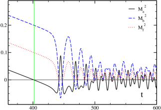
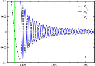
Figure 1: Evolution at the transition between the slow roll and the intermediate period, for $\kappa=0.1$ and $\phi_{0}(0)=4$.

Figure 2: Evolution at the transition between the slow roll and the intermediate period, for $\kappa=0.1$ and $\phi_{0}(0)=64$ .

This period takes a time $t_{1}$ which ranges between $50$ for $\kappa=0.1$ and low excitations and several thousand for $\kappa=0.001$ and large initial value of $\phi_{0}$. The evolution is mostly classical, the fluctuations remain very small. This period ends once the mass squared of the scalar ($a$ field) fluctuations gets negative and the system enters the spinodal regime; this is the usual end of the slow roll phase, marked in the figures as a vertical line at $t=402$ for $\phi_{0}(0)=4$ and at $t=1374$ for $\phi_{0}(0)=64$. The behaviour of the masses in this transition region is displayed in Figs. 2 and 2 for small and large initial exctitations, respectively. ${\cal M}_{a}^{2}$ gets negative first, then the strong increase in the $a$ field fluctuations drives ${\cal M}_{b}^{2}$ to negative values. Subsequently ${\cal M}_{a}^{2}$ and ${\cal M}_{b}^{2}$ oscillate around zero with alternating signs. After a few oscillations ${\cal M}_{b}^{2}$ remains positive while ${\cal M}_{a}^{2}$ continues between positive and negative values. We have entered the second stage of evolution.

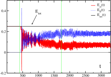
Figure 3: Evolution of the classical and fluctuation energies after the slow roll period. for $\kappa=0.1$ and $\phi_{0}(0)=4$.

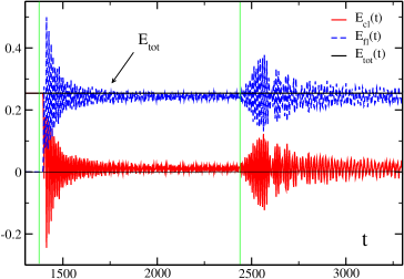
Figure 4: Evolution at the classical and fluctuation energy densities after slow period. for $\kappa=0.1$ and $\phi_{0}(0)=64$.

The point where ${\cal M}_{a}^{2}$ becomes negative marks the end of inflation. At this point the energy density ${\cal E}$ of the classical fields is transferred to the quantum fluctuations, and the pressure, which was essentially equal to $-{\cal E}$ in the inflationary phase becomes the one of a massive or massless gas (see e.g. [33] of an out-of-equilibrium analysis). This transfer of energy density can be seen in Figs. 3 and 4 for small and large initial excitiations, respectively, while it takes a very long time for small excitations. We will see, however, that the evolution of the classical fields towards the classical minimum of the potential will take a long time and is not as instantaneous as often assumed.

If the Hubble expansion were taken into account, the evolution during the slow roll stage would be modified essentially. So our numerical results for this period are not really relevant, they mostly set an initial condition for the second stage, which is characterized by the emergence of the quantum fluctuations.

4.2 Time evolution II: the intermediate period.

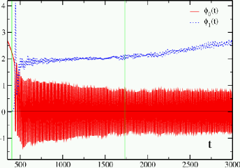
Figure 5: Evolution of the classical fields during the intermediate period for $\kappa=0.1$ and $\phi_{0}(0)=4$.

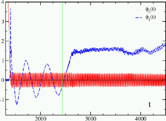
Figure 6: Evolution of the classical fields during the intermediate period, for $\kappa=0.1$ and $\phi_{0}(0)=64$.

In the intermediate period there are two qualitatively different kinds of evolution. For small excitations $\phi_{0}(0)$ the waterfall field $\phi_{1}$ decides to move either into the positive or the negative direction and attains some average value $\bar{\phi}_{1}$ whose absolute value is smaller than the tree level vacuum expectation value $v$. We call this the “broken symmetry phase”. For large excitations $\phi_{0}$ the waterfall field oscillates around zero. We call this the “symmetric phase”. Such a phenomenon has similarly observed in Ref. [26], we discuss it in more detail below. We display the behaviour of the classical fields during this second and the early third period in Figs. 5 and 6 for low and high initial excitation, respectively.

The quantum fluctuations start developing right after entering the spinodal regime. The fermion fluctuations remain very small throughout. The $a$ amplitudes have initially developed exponentially in a low momentum band and ${\cal F}_{a}$ has reached large values right away. Subsequently these fluctuations develop only very slowly, though ${\cal M}_{a}^{2}$ oscillates around zero and therefore becomes negative periodically. This entails an exponential evolution in the low momentum band. However, the periods of exponential evolution alternate with periods where ${\cal M}_{a}^{2}>0$; these intermittent periods modify the initial conditions for the next exponential evolution. So we have neither parametric resonance nor a spinodal evolution and the fluctuation integral ${\cal F}_{a}$ does not evolve significantly.

The squared mass of the $b$ field fluctuations oscillates around some positive value. So they could develop by parametric resonance. A resonance peak can indeed be seen at the beginning of, and during the second period. However, the amplitude of the mass oscillations is small and is of course not cleanly periodic. So the resonance does not evolve efficiently.

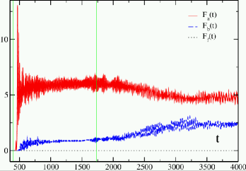
Figure 7: Evolution of the classical fields during the intermediate period for $\kappa=0.1$ and $\phi_{0}(0)=4$.

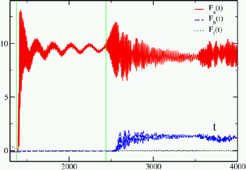
Figure 8: Evolution of the classical fields during the intermediate period, for $\kappa=0.1$ and $\phi_{0}(0)=64$.

We display the evolution of the fluctuation integrals during the second and early third period in Figs. 7 and 8, for small and large initial values of $\phi_{0}$, respectively.

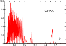
Figure 11: Momentum spectra for the fluctuations of the fields $a$ (left) and $b$ (right) after the intermediate period, for $\kappa=0.1$ and $\phi_{0}(0)=4$.

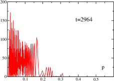
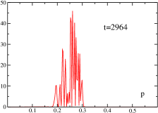
Figure 12: Momentum spectra for the fluctuations of the fields $a$ (left) and $b$ (right) right after the intermediate period, for $\kappa=0.1$ and $\phi_{0}(0)=64$.

Right after the intermediate period the structure of the momentum spectra still displays the same features as in the early stage of this period. They just have become somewhat irregular. They are displayed in Figs. 11 and 12 for small and large initial values of $\phi_{0}$.

4.3 Time evolution III: The late time behaviour

The intermediate period ends with a second strong evolution of the quantum fluctuations, this time including those of the $b$ fields. With the decrease of the field $\phi_{0}$, the increase of $\phi_{1}$ and of $<a^{2}>$ the squared mass ${\cal M}_{b}^{2}$ is, at some point, driven again to negative values, see Eq. (28). The time at which this occurs is marked by a vertical line, at $t=1733$ for $\phi_{0}(0)=4$ and $t=2438$ for $\phi_{0}(0)=64$. Of course the increase of the $b$ fluctuations drives the $b$ mass back to positive values, but then the $a$ mass gets negative again, and so on. This behaviour at the onset of the late time regime is displayed in Figs. 13. The vertical line marks the time where ${\cal M}_{b}^{2}$ starts taking negative values again.

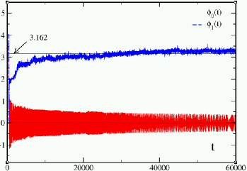
Figure 14: Evolution of the classical fields during the intermediate period for $\kappa=0.1$ and $\phi_{0}(0)=4$.

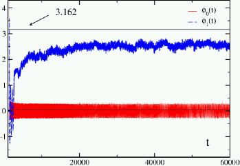
Figure 15: Evolution of the classical fields during the intermediate period, for $\kappa=0.1$ and $\phi_{0}(0)=64$.

Now the $b$ field fluctuations develop significantly. This entails strong fluctuations in all squared masses and a characteristic change in the evolution of the waterfall field. While in the intermediate period it keeps oscillating more or less regularly around zero (symmetric phase, high excitations) or some finite value (broken symmetry phase, low excitations), it now starts shifting towards the classical minimum $\phi_{1}=v$ in quite an irregular motion. The shift is very slow and the motion does not display any periodic oscillations. So the out-of-equilibrium effective potential (if at all one may use such a term) seems to be quite flat, and the motion seems to be determined by stochastic forces instead of well-defined harmonic forces. This is displayed in Figs. 14 and 15. The stochastic behaviour may originate on the one hand from a parametric resonance that is strongly disturbed by the presence and variation of different time scales. On the other hand the oscillations of ${\cal M}_{a}^{2}$ and ${\cal M}_{b}^{2}$ around zero naturally lead to a diffusion process by the alternation of oscillating and exponential time evolution.

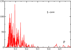
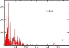
Figure 16: Momentum spectra for the fluctuations of the fields $a$ (left) and $b$ (right) at late times, for $\kappa=0.1$ and $\phi_{0}(0)=4$.

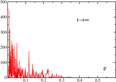
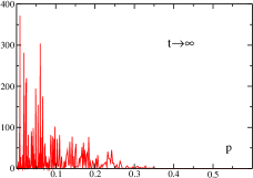
Figure 17: Momentum spectra for the fluctuations of the fields $a$ (left) and $b$ (right) at late times, for $\kappa=0.1$ and $\phi_{0}(0)=64$.

In this late time period both ${\cal M}_{a}^{2}$ and ${\cal M}_{b}^{2}$ oscillate around zero. So, for the low momentum modes the effective frequency takes real and imaginary values in intermittent time intervals. As before for the fluctuations of the $a$ field we get now for both scalar fields a process where an exponential behaviour alternates with an oscillating evolution, which changes initial conditions for the next exponential evolution. This time the amplitudes of oscillation for ${\cal M}_{a/b}^{2}$ are larger, the process becomes more effective and leads to a strong increase of the fluctuation integrals, as mentioned above. At the same time the momentum spectra loose entirely their characteristic features related to parametric resonance and/or spinodal evolution. They are concentrated at small momenta and fall off rapidly with momentum. These spectra are displayed in Fig. 16 for $\phi_{0}(0)=4$ and in Fig. 17 for $\phi_{0}(0)=64$.

This third period of evolution shows novel features that deserve to be analyzed in more detail. Without the pseudoscalar superpartner, the system remains in the “symmetric” and “broken symmetry” phases [26], here the waterfall field always evolves towards of one of its classical minima at late times. The stochastic behaviour contrasts with the spinodal or parametric resonance regimes and seems to represent a new kind of behaviour specific of multifield quantum systems.

4.4 A phase transition

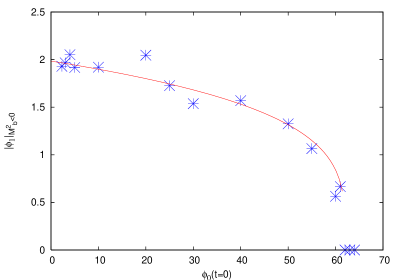
Figure 18: Averages of the waterfall field in the intermediate period as function of the initial value $\phi_{0}(0)$, for $\kappa=0.1$.

As we have discussed previously the system behaves in two different ways in the intermediate stage: for small excitations the field $\phi_{1}$ shifts towards the direction of one of the classical minima and oscillates in an irregular way around some mean value which depends on the initial excitation. With increasing initial excitation this mean value becomes smaller and above some critical value it becomes zero. This can be seen as a phase transition, with a symmetric phase for large excitation, i.e. large energy densities. We plot, in Fig. 18

this average value as a function of $\phi_{0}(0)$, for $\kappa=0.1$. As the intermediate period only lasts for a finite time, this average is not really well-defined and is read off by inspection. This explains why the values are somewhat scattered. The plot looks like the phase diagram of a second order phase transition, with $\phi_{0}(0)$ as the “temperature” and $\bar{\phi}_{1}$ as the order parameter. The diagram may be compared with similar figures in other work on models with spontaneous symmetry breaking, like Fig. 11 of Ref. [26], Figs. 6-8 in Ref. [34] and Fig. 4 in [35]. In contrast to the models studied previously, for the present model the waterfall field always ends up at $|\phi_{1}|\simeq v$ as $t\to\infty$, but this is a process that takes a long time.

4.5 The effective potential

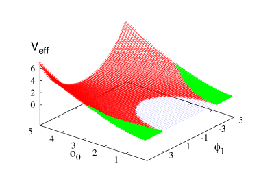
Figure 19: The equilibrium effective potential for $\kappa=0.1$.

As we have noticed, the motion of the waterfall fields towards its tree level expectation value does not seem to be driven by any strong force. The slow and somewhat irregular motion rather suggests an effective potential that is quite flat, with a small inclination towards $\phi_{1}=\pm v$. Indeed it is well-known that for $\phi^{4}$ theory with $SO(N)$ symmetry and a Mexican hat potential the central region $|\vec{\phi}|<v$ becomes flat, once quantum corrections are taken into account in the large-$N$ limit. Here a similar phenomenon takes place. The effective potential for our model in the large-$N$ limit is derived in Appendix B and is displayed in Fig. 19.

The region in the center is flat in the $\phi_{1}$-direction, it is the region $B$ defined in Appendix B where the gap equation would yield the unphysical solution ${\cal M}_{a}^{2}<0$. At $\phi_{0}=0$ it is bounded by $\phi_{1}=\pm v$, i.e. by $\pm 1/\sqrt{\kappa}$ in our mass units. One sees that the spinodal region has disappeared and the effective potential has become flat in the central region. Of course this is the equilibrium effective potential, here its flatness seems to be “realized dynamically” by the motion of the waterfall field, as it was found in a somewhat different way for the $SO(N)$ model in Ref. [35].

5 Summary and Conclusions

We have studied here a supersymmetric hybrid model in a large-$N$ approximation. The motivation for this research was the interest in the rôle of quantum fluctuations in the evolution near and after the end of the slow roll regime. In generalizing previous work we have taken into account the fluctuations of all superpartners of the waterfall field. While the fermion field fluctuations remain small in general and they mainly play their rôle in the renormalization, the fluctuations of the scalar and pseudoscalar fields show an interesting interplay, resulting in a peculiar behaviour of the classical waterfall field which is different from the behaviour found in previous analyses:

(i) the evolution after the end of slow roll displays two stages: in the first (intermediate) stage the behaviour is similar to the one found previously for the hybrid model with quantum backreaction [26], only the scalar field fluctuations develop and the system goes to a symmetric phase at high excitations, and to a broken symmetry phase at low excitation. In the second stage (late time) the fluctuations of the pseudoscalar superpartner start developing and the waterfall fields moves towards its classical vacuum expectation value.

(ii) the dynamics of the fluctuations is, apart from an initial spinodal evolution of the scalar field fluctuations, neither dominated by the spinodal instability nor by parametric resonance. On the one hand a clean parametric resonance is suppressed by the presence of multiple time scales, there is no simple periodic motion in the background fields. On the other hand the oscillations of the effective squared masses ${\cal M}_{a}^{2}$ and ${\cal M}_{b}^{2}$ around zero lead to a kind of diffusive behaviour for the (dominant) low energy modes. Within short time intervals exponential and oscillatory evolution alternate, the fluctuations and their integrals vary in a stochastic way. This behaviour is transmitted to the waterfall field whose motion is an irregular drift towards its classical vacuum expectation value.

We think that these findings warrant a further consideration of the hybrid model in its supersymmetric extension. The following issues would be of interest and could be the subject for further studies:

(i) how does the behaviour change in the presence of Hubble expansion, i.e. in a FRW universe? This will lead to a damping of the classical field and of the fluctuations. While the Hubble expansion is often neglected in studies of preheating, here, right at the end of inflation, it can be expected to lead to significant modifications. This is also the reason for which we do not want to draw premature conclusions from our numerical results. The techniques for handling the dynamics in an expanding universe, including renormalization, have been developed previously [36, 37].

(ii) does the peculiar dynamical behaviour lead to imprints on the CMBR spectrum? In particular, nongaussianity may arise in such multifield models from the evolution near the end of inflation, see [22] and references therein.

(iii) is the peculiar behaviour a genuine property of a supersymmetric model with its specific structure of the mass terms, or is it simply a consequence of the presence of many different time scales, or both?

We plan to study these questions in the near future.

Appendix A Renormalization

The fluctuation integrals introduced in section 2 are divergent. In dimensional regularization we find

$$<a^{2}> = {\cal F}_{a}=-I_{-3}(m^{2}){\cal M}_{a}^{2}+{\cal F}_{a}^{\rm fin}\;,$$

$$<b^{2}> = {\cal F}_{b}=-I_{-3}(m^{2}){\cal M}_{b}^{2}+{\cal F}_{b}^{\rm fin}\;,$$ (A1)

$$<\bar{\psi}\psi> = {\cal F}_{f}=I_{-3}(m^{2})\left[2\ddot{\cal M}_{f}+4{\cal M}_{f}^{3}\right]+{\cal F}_{f}^{\rm fin}\;.$$

Here

$${\cal F}_{a}^{\rm fin} = -\frac{1}{16\pi^{2}}m_{a0}^{2}-\frac{{\cal M}_{a}^{2}}{16\pi^{2}}\ln\frac{m^{2}}{m_{a0}^{2}}+{\cal F}_{a}^{\rm sub}\;,$$ (A2)

$${\cal F}_{b}^{\rm fin} = -\frac{1}{16\pi^{2}}m_{b0}^{2}-\frac{{\cal M}_{b}^{2}}{16\pi^{2}}\ln\frac{m^{2}}{m_{b0}^{2}}+{\cal F}_{b}^{\rm sub}\;,$$ (A3)

$${\cal F}_{f}^{\rm fin} = \frac{1}{4\pi^{2}}m_{f0}^{2}{\cal M}_{f}+\frac{1}{8\pi^{2}}\ln\frac{m^{2}}{m_{f0}^{2}}\left(2{\cal M}_{f}^{3}+\sqrt{2}\kappa\ddot{\phi}_{0}\right)+{\cal F}_{f}^{\rm sub}\;,$$ (A4)

with

$${\cal F}_{a/b}^{\rm sub}(t)=\int\!\frac{d^{3}k}{(2\pi)^{3}2\omega_{a/b0}}\,\left[|f^{ab}_{k}(t)|^{2}+\frac{{\cal V}_{a/b}}{2\omega_{a/b0}^{2}}\right]$$ (A5)

and [31]

$${\cal F}_{f}^{\rm sub}(t) = -2\int\!\frac{d^{3}k}{(2\pi)^{3}}\,\left[1-\frac{\omega_{f0}-m_{f0}}{\omega_{f0}}|f_{k}^{\psi}(t)|^{2}-\frac{{\cal M}_{f}(t)}{\omega_{f0}}\right.$$ (A6)

$$\left.+\frac{\ddot{\cal M}_{f}(t)}{4\omega_{f0}^{3}}+\frac{{\cal M}_{f}(t)({\cal M}_{f}^{2}(t)-m_{f0}^{2})}{2\omega_{f0}^{3}}\right]\;.$$

We introduce the renormalization constants $Z_{i}$ as follows:

$$\phi_{0} \to Z_{0}\phi_{0}$$

$$\phi_{1} \to Z_{1}\phi_{1}$$ (A7)

$$\kappa \to Z_{\kappa}\kappa$$

$$v \to Z_{1}v$$

The fluctuation fields $a,b,\psi$ are likewise multiplied by $Z_{1}$ as they belong to the same superfield as $\phi_{1}$, more precisely they belong to the same $SO(N)$ multiplet of superfields as $\phi_{1}$. The vacuum expectation value has been rescaled as $\phi_{1}$ in order to preserve its tree level interpretation.

We first discuss the gap equation. It takes the form

$${\cal M}_{-}^{2}=Z_{\kappa}^{2}Z_{1}^{2}\kappa^{2}\left[\phi_{1}^{2}-v^{2}-2I_{-3}(m^{2}){\cal M}_{-}^{2}+{\cal F}_{-}^{\rm fin}\right]$$ (A8)

with ${\cal F}_{-}^{\rm fin}={\cal F}_{a}^{\rm fin}-{\cal F}_{b}^{\rm fin}$. This can be written as

$${\cal M}_{-}^{2}(1+2\kappa^{2}Z_{\kappa}^{2}Z_{1}^{2}I_{-3}(m^{2}))=Z_{\kappa}^{2}Z_{1}^{2}\kappa^{2}\left[\phi_{1}^{2}-v^{2}+{\cal F}_{-}^{\rm fin}\right]\;.$$ (A9)

In order to obtain the finite equations in the same form as the unrenormalized ones we have to put $1+2\kappa^{2}Z_{\kappa}^{2}Z_{1}^{2}I_{-3}(m^{2})$ equal to $Z_{\kappa}^{2}Z_{1}^{2}$ or

$$Z_{\kappa}^{2}Z_{1}^{2}=\frac{1}{1-2\kappa^{2}I_{-3}(m^{2})}$$ (A10)

and obtain the finite gap equation

$${\cal M}_{-}^{2}=\kappa^{2}\left(\phi_{1}^{2}-v^{2}+{\cal F}_{-}^{\rm fin}\right)\;.$$ (A11)

Next we consider the equations of motion. We start with the one for $\phi_{1}$, which after divison by $Z_{1}$ takes the form

$$\ddot{\phi}_{1}+2Z_{\kappa}^{2}Z_{0}^{2}\kappa^{2}\phi_{0}^{2}\phi_{1}+{\cal M}_{-}^{2}\phi_{1}=0\;.$$ (A12)

As ${\cal M}_{-}^{2}$ is already finite we have to set

$$Z_{0}Z_{\kappa}=1\;.$$ (A13)

This entails that also the renormalized equation of motion for the field $\psi$ retains its bare form. We now consider the equation of motion for $\phi_{0}$. It becomes, after dividing by $Z_{0}$ which is equivalent of multiplying with $Z_{\kappa}$

$$\ddot{\phi}_{0}+Z_{\kappa}^{2}Z_{1}^{2}\left[2\kappa^{2}\phi_{0}\phi_{1}^{2}+2\kappa^{2}\phi_{0}(<a^{2}>+<b^{2}>)+\frac{1}{\sqrt{2}}\kappa<\bar{\psi}\psi>\right]=0\;.$$ (A14)

We use the relations (A1) to rewrite this as

$$\ddot{\phi}_{0}+Z_{\kappa}^{2}Z_{1}^{2}\left[2\kappa^{2}\phi_{0}(\phi_{1}^{2}-4I_{-3}(m^{2})\kappa^{2}\phi_{0}^{2}+{\cal F}_{+}^{\rm fin})\right.$$

$$\left.+\frac{1}{\sqrt{2}}\kappa I_{-3}(m^{2})(2\sqrt{2}\kappa\ddot{\phi}_{0}+8\sqrt{2}\kappa^{3}\phi_{0}^{3})+\frac{1}{\sqrt{2}}\kappa{\cal F}_{f}^{\rm fin}\right]=0\;,$$ (A15)

where ${\cal F}_{+}^{\rm fin}={\cal F}_{a}^{\rm fin}+{\cal F}_{b}^{\rm fin}$. In order to obtain again the tree level relation with finite quantities we have to put

$$1+2Z_{\kappa}^{2}\kappa^{2}Z_{1}^{2}I_{-3}(m^{2})=Z_{\kappa}^{2}Z_{1}^{2}\;.$$ (A16)

which is the same relation we have obtained previously.

Up to now only the products $Z_{0}Z_{\kappa}$ and $Z_{1}Z_{\kappa}$ are fixed. We now consider the renormalization of the energy. The total energy density written in terms of the bare fields and couplings is given by

$${\cal E} = \frac{1}{2}\dot{\phi}_{0}^{2}+\frac{1}{2}\dot{\phi}_{1}^{2}+\kappa^{2}\phi_{0}^{2}\phi_{1}^{2}+\frac{\kappa^{2}}{4}\left(\phi_{1}^{2}-v^{2}\right)^{2}$$

$$+<\frac{1}{2}\dot{a}^{2}+\frac{1}{2}k^{2}a^{2}+\frac{1}{2}{\cal M}_{a}^{2}a^{2}>$$

$$+<\frac{1}{2}\dot{b}^{2}+\frac{1}{2}k^{2}b^{2}+\frac{1}{2}{\cal M}_{b}^{2}a^{2}>$$

$$-\frac{\kappa^{2}}{4}\left(<a^{2}>-<b^{2}>\right)^{2}+\frac{1}{2}\psi^{\dagger}\left(\vec{\alpha}\vec{k}+\beta{\cal M}_{f}\right)\psi\;.$$

In terms of the renormalized fields this becomes

$${\cal E} = \frac{1}{2}Z_{0}^{2}\dot{\phi}_{0}^{2}+\frac{1}{2}Z_{1}^{2}\dot{\phi}_{1}^{2}+Z_{0}^{2}Z_{1}^{2}Z_{\kappa}^{2}\kappa^{2}\phi_{0}^{2}\phi_{1}^{2}+Z_{1}^{4}Z_{\kappa}^{2}\frac{\kappa^{2}}{4}\left(\phi_{1}^{2}-v^{2}\right)^{2}$$

$$+Z_{1}^{2}<\frac{1}{2}\dot{a}^{2}+\frac{1}{2}k^{2}a^{2}+\frac{1}{2}{\cal M}_{a}^{2}a^{2}>$$

$$+Z_{1}^{2}<\frac{1}{2}\dot{b}^{2}+\frac{1}{2}k^{2}b^{2}+\frac{1}{2}{\cal M}_{b}^{2}a^{2}>$$

$$-Z_{\kappa}^{2}Z_{1}^{4}\frac{\kappa^{2}}{4}\left(<a^{2}>-<b^{2}>\right)^{2}+\frac{1}{2}Z_{1}^{2}\psi^{\dagger}\left(\vec{\alpha}\vec{k}+\beta{\cal M}_{f}\right)\psi\;.$$

Separating the divergent parts we have

$${\cal E}_{\rm fl,a} = <\frac{1}{2}\dot{a}^{2}+\frac{1}{2}k^{2}a^{2}+{\cal M}_{a}^{2}a^{2}>$$ (A19)

$$= -\frac{1}{4}I_{-3}(m^{2}){\cal M}_{a}^{4}+{\cal E}_{\rm fl,a}^{\rm fin}\;,$$

$${\cal E}_{\rm fl,b} = <\frac{1}{2}\dot{b}^{2}+\frac{1}{2}k^{2}b^{2}+{\cal M}_{b}^{2}b^{2}>$$ (A20)

$$= -\frac{1}{4}I_{-3}(m^{2}){\cal M}_{b}^{4}+{\cal E}_{\rm fl,b}^{\rm fin}\;,$$

$${\cal E}_{\rm fl,f} = \frac{1}{2}\bar{\psi}\left(\vec{\alpha}\vec{k}+\beta{\cal M}_{f}\right)\psi$$ (A21)

$$= \frac{1}{2}I_{-3}(m^{2})\left[2\kappa^{2}\dot{\phi}_{0}^{2}+4\kappa^{4}\phi_{0}^{4}\right]+{\cal E}_{\rm fl,f}^{\rm fin}\;.$$

Here

$${\cal E}_{\rm fl,a}^{\rm fin} = \frac{1}{128\pi^{2}}m_{a0}^{4}-\frac{1}{32\pi^{2}}m_{a0}^{2}{\cal M}_{a}^{2}-\frac{1}{64\pi^{2}}\ln\frac{m^{2}}{m_{a0}^{2}}{\cal M}_{a}^{4}+{\cal E}_{\rm fl,a}^{\rm sub}\;,$$ (A22)

$${\cal E}_{\rm fl,b}^{\rm fin} = \frac{1}{128\pi^{2}}m_{b0}^{4}-\frac{1}{32\pi^{2}}m_{b0}^{2}{\cal M}_{b}^{2}-\frac{1}{64\pi^{2}}\ln\frac{m^{2}}{m_{b0}^{2}}{\cal M}_{b}^{4}+{\cal E}_{\rm fl,b}^{\rm sub}\;,$$ (A23)

$${\cal E}_{\rm fl,f}^{\rm fin} = -\frac{1}{64\pi^{2}}m_{f0}^{4}+\frac{1}{16\pi^{2}}m_{f0}^{2}{\cal M}_{f}^{2}+\frac{1}{32\pi^{2}}\ln\frac{m^{2}}{m_{f0}^{2}}({\cal M}_{f}^{4}+\dot{\cal M}_{f}^{2})$$ (A24)

$$+{\cal E}_{\rm fl,f}^{\rm sub}\;,$$

where the superscript ’sub’ refers to the subtracted fluctuation integrals which can be found in detailed form in Refs. [31, 30].

The divergent parts of the three fluctuation energies combine into

$${\cal E}_{\rm fl}^{\rm div} = -\frac{1}{4}I_{-3}(m^{2})\left[{\cal M}_{a}^{4}+{\cal M}_{b}^{4}-2{\cal M}_{f}^{4}\right]+I_{-3}(m^{2})\kappa^{2}\dot{\phi}_{0}^{2}$$ (A25)

$$= -\frac{1}{2}I_{-3}(m^{2}){\cal M}_{-}^{4}+I_{-3}(m^{2})\kappa^{2}\dot{\phi}_{0}^{2}\;.$$

In the total energy the fluctuations contribute a term

$$-\frac{Z_{1}^{2}}{2}I_{-3}(m^{2}){\cal M}_{-}^{4}+Z_{1}^{2}{\cal E}_{\rm fl}^{\rm fin}+Z_{1}^{2}I_{-3}(m^{2})\kappa^{2}\dot{\phi}_{0}^{2}\;.$$ (A26)

If we want the energy density to keep its bare form in terms of finite quantities we have to set $Z_{1}=1$. Then in Eq. (A) the second and third term have already their bare form in terms of renormalized quantities. The first term and $\dot{\phi}_{0}^{2}$-term in the divergent fluctuation energies combine into

$$\frac{1}{2}\left(Z_{0}^{2}+2\kappa^{2}I_{-3}(m^{2})\right)\dot{\phi}_{0}^{2}\;.$$ (A27)

This takes the canonical form if

$$Z_{0}^{2}=1-2\kappa^{2}I_{-3}(m^{2})\;.$$ (A28)

This is consistent with Eq (A13) if

$$Z_{\kappa}^{2}=Z_{0}^{-2}=\frac{1}{1-2\kappa^{2}I_{-3}(m^{2})}$$ (A29)

and this is also consistent with Eq. (A10) if $Z_{1}=1$ as obtained previously.

The fourth term in the energy density combines with the seventh term into

$$Z_{\kappa}^{2}\frac{\kappa^{2}}{4}(\phi_{1}^{2}-v^{2})^{2}-Z_{\kappa}^{2}\frac{\kappa^{2}}{4}\left(<a^{2}>-<b^{2}>\right)^{2}$$

$$=\frac{1}{4}{\cal M}_{-}^{2}\left[\phi_{1}^{2}-v^{2}-(<a>^{2}-<b>^{2})\right]$$

$$=\frac{1}{2}{\cal M}_{-}^{2}\left(\phi_{1}^{2}-v^{2}\right)-\frac{1}{4Z_{\kappa}^{2}\kappa^{2}}{\cal M}_{-}^{4}$$ (A30)

$$=\frac{1}{2}{\cal M}_{-}^{2}\left(\phi_{1}^{2}-v^{2}\right)-\frac{1}{4\kappa^{2}}{\cal M}_{-}^{4}+\frac{1}{2}I_{-3}{\cal M}_{-}^{4}\;.$$

The last term in the last equation cancels with the ${\cal M}_{-}^{4}$-term in the fluctuation energies. So with the choices of the $Z_{i}$ given above the energy density and the equations of motion are finite. The energy density now becomes

$${\cal E}=\frac{1}{2}\dot{\phi}_{0}^{2}+\frac{1}{2}\dot{\phi}_{1}^{2}+\kappa^{2}\phi_{0}^{2}\phi_{1}^{2}+{\cal E}_{\rm fl}^{\rm fin}+\frac{1}{2}{\cal M}_{-}^{2}\left(\phi_{1}^{2}-v^{2}\right)-\frac{1}{4\kappa^{2}}{\cal M}_{-}^{4}\;.$$ (A31)

Here the gap equation has been implemented. Indeed, variation with respect to ${\cal M}_{-}^{2}$ yields the gap equation

$${\cal M}_{-}^{2}(t)=\kappa^{2}\left(\phi_{1}^{2}(t)-v^{2}+2\frac{\delta{\cal E}_{\rm fl}^{\rm fin}}{\delta{\cal M}_{-}^{2}(t)}\right)\;.$$ (A32)

The equations of motion for the fluctuations as well as the one for $\phi_{1}$ have exactly the same form as the bare equations if we use the masses ${\cal M}_{a}^{2},{\cal M}_{b}^{2},{\cal M}_{f}^{2}$ and ${\cal M}_{-}^{2}$. The equation of motion for $\phi_{0}$ has the form

$$\ddot{\phi}_{0}+2\kappa^{2}\phi_{0}\left(\phi_{1}^{2}+{\cal F}_{+}^{\rm fin}\right)+\frac{\kappa}{\sqrt{2}}{\cal F}_{f}^{\rm fin}=0\;.$$ (A33)

This equation of motion cannot be solved trivially with respect to $\ddot{\phi}_{0}$ as ${\cal F}_{f}^{\rm fin}$ explicitly contains $\ddot{\phi}_{0}$. So the term $\ddot{\phi}_{0}$ appears with a factor

$${\cal C}_{0}=1+2\frac{\kappa^{2}}{16\pi^{2}}\ln\frac{m^{2}}{m_{f0}^{2}}\;.$$ (A34)

Likewise the finite gap equation contains ${\cal M}_{-}^{2}$ on both sides. At $t=0$ this is not a problem as it is solved by iteration anyway. But if we want to express ${\cal M}_{-}^{2}$ at finite $t$ by the subtracted fluctuation integrals we have to write it in a modified form. We have

$${\cal M}_{-}^{2} = \kappa^{2}\left[\phi_{1}^{2}-v^{2}-\frac{1}{16\pi^{2}}(m_{a0}^{2}-m_{b0}^{2})+\frac{{\cal M}_{f}^{2}}{16\pi^{2}}\ln\frac{m^{2}_{a0}}{m^{2}_{b0}}\right.$$ (A35)

$$\left.+\frac{{\cal M}_{-}^{2}}{16\pi^{2}}\ln\frac{m^{2}_{a0}m^{2}_{b0}}{m^{4}}+{\cal F}_{a}^{\rm sub}-{\cal F}_{b}^{\rm sub}\right]\;,$$

or

$${\cal M}_{-}^{2}={\cal C}_{-}\kappa^{2}\left[\phi_{1}^{2}-v^{2}-\frac{1}{16\pi^{2}}(m_{a0}^{2}-m_{b0}^{2})+\frac{{\cal M}_{f}^{2}}{16\pi^{2}}\ln\frac{m^{2}_{a0}}{m^{2}_{b0}}+{\cal F}_{a}^{\rm sub}-{\cal F}_{b}^{\rm sub}\right]\;,$$ (A36)

with

$${\cal C}_{-}=\frac{1}{\displaystyle 1-2\frac{\kappa^{2}}{16\pi^{2}}\ln\frac{m_{a0}m_{b0}}{m^{2}}}\;.$$ (A37)

Appendix B The large-N effective potential

The energy density for constant fields is the effective potential. This effective potential is obtained in the $2PI$ formalism by maximizing with respect to ${\cal M}_{-}^{2}$ the action as a functional of the fields and masses. In our model and in the large-$N$ approximation this action takes the form

$${\cal V}({\cal M}_{-}^{2},\phi_{0},\phi_{1}) = \kappa^{2}\phi_{0}^{2}\phi_{1}^{2}+\frac{1}{2}{\cal M}_{-}^{2}(\phi_{1}^{2}-v^{2})-\frac{1}{4\kappa^{2}}{\cal M}_{-}^{4}$$

$$-\frac{{\cal M}_{a}^{4}}{128\pi^{2}}\left(3+2\ln\frac{m^{2}}{{\cal M}_{a}^{2}}\right)-\frac{{\cal M}_{b}^{4}}{128\pi^{2}}\left(3+2\ln\frac{m^{2}}{{\cal M}_{b}^{2}}\right)$$

$$+\frac{{\cal M}_{f}^{4}}{64\pi^{2}}\left(3+2\ln\frac{m^{2}}{{\cal M}_{f}^{2}}\right)\;.$$

Variation with respect to the mass ${\cal M}_{-}^{2}$ yields the gap equation:

$$\frac{\partial{\cal V}({\cal M}_{-}^{2},\phi_{0},\phi_{1})}{\partial{\cal M}_{-}^{2}} = \frac{1}{2}(\phi_{1}^{2}-v^{2})-\frac{1}{2\kappa^{2}}{\cal M}_{-}^{2}$$

$$-\frac{{\cal M}_{a}^{2}}{32\pi^{2}}\left(1+\ln\frac{m^{2}}{{\cal M}_{a}^{2}}\right)+\frac{{\cal M}_{b}^{2}}{32\pi^{2}}\left(1+\ln\frac{m^{2}}{{\cal M}_{b}^{2}}\right)=0\;,$$

or

$${\cal M}_{-}^{2}=\kappa^{2}\left[\phi_{1}^{2}-v^{2}-\frac{{\cal M}_{a}^{2}}{16\pi^{2}}\left(1+\ln\frac{m^{2}}{{\cal M}_{a}^{2}}\right)+\frac{{\cal M}_{b}^{2}}{16\pi^{2}}\left(1+\ln\frac{m^{2}}{{\cal M}_{b}^{2}}\right)\right]\;.$$ (B2)

The solution of this equation is to be inserted into ${\cal V}({\cal M}_{-}^{2},\phi_{0},\phi_{1})$ in order to obtain $V_{\rm eff}(\phi_{0},\phi_{1})$.

The gap equation has a solution only in a restricted part of the $\phi_{0},\phi_{1}$ plane. Both ${\cal M}_{a}^{2}$ and ${\cal M}_{b}^{2}$ have to be positive, and such a solution does not exist everywhere. The boundaries of this region are traced by the conditions ${\cal M}_{a}^{2}=0$ and ${\cal M}_{b}^{2}=0$. Outside this region the maximum of the variational potential is to be taken at the boundaries. In spontaneously broken $\phi^{4}$ theory at large $N$ this construction leads to a flat potential in the central region $|\vec{\phi}|<v$ of the “Mexican hat” (see related discussions in Ref. [38]).

Here the boundaries of the regions where the gap equation yields the unphysical solutions ${\cal M}_{b}^{2}<0$ (region A) and ${\cal M}_{a}^{2}<0$ (region B) are determined by the conditions

$$(\partial A)\;\; {\cal M}_{b}^{2}=0\;\;;\;\;{\cal M}_{-}^{2}=2\kappa^{2}\phi_{0}^{2}\;\;;\;\;{\cal M}_{a}^{2}=4\kappa^{2}\phi_{0}^{2}\;,$$ (B3)

$$(\partial B)\;\; {\cal M}_{a}^{2}=0\;\;;\;\;{\cal M}_{-}^{2}=-2\kappa^{2}\phi_{0}^{2}\;\;;\;\;{\cal M}_{b}^{2}=4\kappa^{2}\phi_{0}^{2}\;.$$ (B4)

In the regions $A$ and $B$ the masses ${\cal M}_{a}^{2}$ and ${\cal M}_{b}^{2}$, respectively, retain their boundary values, i.e. zero. Then the effective potential can be given analytically as

$$V^{A}_{\rm eff} = \kappa^{2}\phi_{0}^{2}\phi_{1}^{2}+\kappa^{2}\phi_{0}^{2}(\phi_{1}^{2}-v^{2})-\kappa^{2}\phi_{0}^{4}$$ (B6)

$$-\frac{16\kappa^{4}\phi_{0}^{4}}{128\pi^{2}}\left(3+2\ln\frac{m^{2}}{4\kappa^{2}\phi_{0}^{2}}\right)$$

$$+\frac{4\kappa^{4}\phi_{0}^{4}}{64\pi^{2}}\left(3+2\ln\frac{m^{2}}{2\kappa^{2}\phi_{0}^{2}}\right)$$

and

$$V^{B}_{\rm eff} = \kappa^{2}\phi_{0}^{2}\phi_{1}^{2}-\kappa^{2}\phi_{0}^{2}(\phi_{1}^{2}-v^{2})-\kappa^{2}\phi_{0}^{4}$$ (B8)

$$-\frac{16\kappa^{4}\phi_{0}^{4}}{128\pi^{2}}\left(3+2\ln\frac{m^{2}}{4\kappa^{2}\phi_{0}^{2}}\right)$$

$$+\frac{4\kappa^{4}\phi_{0}^{4}}{64\pi^{2}}\left(3+2\ln\frac{m^{2}}{2\kappa^{2}\phi_{0}^{2}}\right)$$

The latter potential is independent of $\phi_{1}$ and replaces the potential in and around the spinodal region.

The conditions $(\partial A)$ and $(\partial B)$ do not determine the regions of validity in terms of the fields $\phi_{0}$ and $\phi_{1}$. A way of obtaining these regions in a numerical code is to solve the gap equation admitting negative values of ${\cal M}_{a}^{2}$ and ${\cal M}_{b}^{2}$, taking the absolute values in the logs. If ${\cal M}_{a}^{2}$ is found to be negative one is in region $B$, if ${\cal M}_{b}^{2}$ is found to be negative one is in region $A$. As long as the potential ${\cal V}$ has just one maximum as a function of ${\cal M}_{-}^{2}$ this recipe is rigorous.

If one omits the fluctuation terms, the region where the potential $V^{B}_{\rm eff}$ is independent of $\phi_{1}$ is the region inside $|\phi_{1}|<\sqrt{v^{2}-2\phi_{0}^{2}}$ which includes the spinodal region.

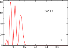
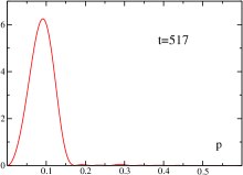
Figure 9: Momentum spectra for the fluctuations of the fields $a$ (left) and $b$ (right) right after slow roll, for $\kappa=0.1$ and $\phi_{0}(0)=4$.

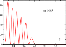
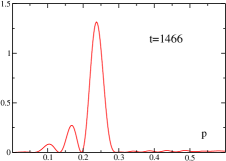
Figure 10: Momentum spectra for the fluctuations of the fields $a$ (left) and $b$ (right) right after slow roll, for $\kappa=0.1$ and $\phi_{0}(0)=64$.

Figure 13: Evolution of the masses at the transition between intermediate and late time regime, for $\kappa=0.1$ and $\phi_{0}(0)=4$.

References

- [1] A. D. Linde, Phys. Lett. B249, 18 (1990).
- [2] A. D. Linde, Phys. Lett. B259, 38 (1991).
- [3] A. D. Linde, Phys. Rev. D49, 748 (1994), [astro-ph/9307002].
- [4] E. J. Copeland, A. R. Liddle, D. H. Lyth, E. D. Stewart and D. Wands, Phys. Rev. D49, 6410 (1994), [astro-ph/9401011].
- [5] J. Garcia-Bellido and A. D. Linde, Phys. Rev. D57, 6075 (1998), [hep-ph/9711360].
- [6] R. Micha and M. G. Schmidt, Eur. Phys. J. C14, 547 (2000), [hep-ph/9908228].
- [7] W. Buchmuller, L. Covi and D. Delepine, Phys. Lett. B491, 183 (2000), [hep-ph/0006168].
- [8] H. P. Nilles, M. Peloso and L. Sorbo, JHEP 04, 004 (2001), [hep-th/0103202].
- [9] T. Asaka, W. Buchmuller and L. Covi, Phys. Lett. B510, 271 (2001), [hep-ph/0104037].
- [10] D. Cormier, K. Heitmann and A. Mazumdar, Phys. Rev. D65, 083521 (2002), [hep-ph/0105236].
- [11] D. H. Lyth and A. Riotto, Phys. Rept. 314, 1 (1999), [hep-ph/9807278].
- [12] J. Garcia-Bellido, D. Y. Grigoriev, A. Kusenko and M. E. Shaposhnikov, Phys. Rev. D60, 123504 (1999), [hep-ph/9902449].
- [13] M. Bastero-Gil, S. F. King and J. Sanderson, Phys. Rev. D60, 103517 (1999), [hep-ph/9904315].
- [14] L. M. Krauss and M. Trodden, Phys. Rev. Lett. 83, 1502 (1999), [hep-ph/9902420].
- [15] G. N. Felder et al., Phys. Rev. Lett. 87, 011601 (2001), [hep-ph/0012142].
- [16] G. N. Felder, L. Kofman and A. D. Linde, Phys. Rev. D64, 123517 (2001), [hep-th/0106179].
- [17] E. J. Copeland, D. Lyth, A. Rajantie and M. Trodden, Phys. Rev. D64, 043506 (2001), [hep-ph/0103231].
- [18] J. Garcia-Bellido, M. Garcia Perez and A. Gonzalez-Arroyo, Phys. Rev. D67, 103501 (2003), [hep-ph/0208228].
- [19] S. Borsanyi, A. Patkos and D. Sexty, Phys. Rev. D66, 025014 (2002), [hep-ph/0203133].
- [20] S. Borsanyi, A. Patkos and D. Sexty, Phys. Rev. D68, 063512 (2003), [hep-ph/0303147].
- [21] L. Alabidi, JCAP 0610, 015 (2006), [astro-ph/0604611].
- [22] N. Barnaby and J. M. Cline, astro-ph/0611750.
- [23] G. R. Dvali, Q. Shafi and R. K. Schaefer, Phys. Rev. Lett. 73, 1886 (1994), [hep-ph/9406319].
- [24] D. Boyanovsky, D. Cormier, H. J. de Vega and R. Holman, Phys. Rev. D55, 3373 (1997), [hep-ph/9610396].
- [25] M. J. Bowick and A. Momen, Phys. Rev. D58, 085014 (1998), [hep-ph/9803284].
- [26] J. Baacke and A. Heinen, Phys. Rev. D69, 083523 (2004), [hep-ph/0311282].
- [27] J. Baacke, D. Cormier, H. J. de Vega and K. Heitmann, Nucl. Phys. B649, 415 (2003), [hep-ph/0110205].
- [28] J. Baacke, D. Cormier, H. J. de Vega and K. Heitmann, Phys. Lett. B520, 317 (2001), [hep-ph/0011395].
- [29] G. R. Dvali, L. M. Krauss and H. Liu, hep-ph/9707456.
- [30] J. Baacke, K. Heitmann and C. Patzold, Phys. Rev. D55, 2320 (1997), [hep-th/9608006].
- [31] J. Baacke, K. Heitmann and C. Patzold, Phys. Rev. D58, 125013 (1998), [hep-ph/9806205].
- [32] V. N. Senoguz and Q. Shafi, Phys. Rev. D71, 043514 (2005), [hep-ph/0412102].
- [33] D. Boyanovsky, H. J. de Vega, R. Holman and J. F. J. Salgado, Phys. Rev. D54, 7570 (1996), [hep-ph/9608205].
- [34] J. Baacke and K. Heitmann, Phys. Rev. D62, 105022 (2000), [hep-ph/0003317].
- [35] D. Boyanovsky, H. J. de Vega, R. Holman and J. Salgado, Phys. Rev. D59, 125009 (1999), [hep-ph/9811273].
- [36] J. Baacke, K. Heitmann and C. Patzold, Phys. Rev. D56, 6556 (1997), [hep-ph/9706274].
- [37] J. Baacke and C. Patzold, Phys. Rev. D62, 084008 (2000), [hep-ph/9912505].
- [38] W. A. Bardeen and M. Moshe, Phys. Rev. D28, 1372 (1983).