Graviton emission from a Gauss-Bonnet brane

Abstract

We study the emission of gravitons by a homogeneous brane with the Gauss-Bonnet term into an Anti de Sitter five dimensional bulk spacetime. It is found that the graviton emission depends on the curvature scale and the Gauss-Bonnnet coupling and that the amount of emission generally decreases. Therefore nucleosynthesis constraints are easier to satisfy by including the Gauss-Bonnet term.

I Introduction

In recent years there has been considerable interest in the suggestion that our universe is a brane: a sub-space embedded in a higher-dimensional bulk spacetime. In these models, ordinary matter is confined to our brane while the gravitational field propagates through the whole spacetime. Of particular importance is the Randall-Sundrum (RS) model, where a single brane is embedded in an infinitely extended Ad$S_{5}$ spacetime RS2 . At low energies, the zero mode of the 5D graviton is localized on the brane, because of the strong curvature of the bulk due to a negative bulk cosmological constant, and 4D gravity is recovered.
 A natural extension of the RS model is to include higher order curvature invariants in the bulk. Such terms arise in the Ads/CFT correspondence as next-to-leading order corrections to the CFT CFT . Particularly, in the heterotic string effective action, the Gauss-Bonnet (GB) term arises as the leading order quantum corrections to gravity. This gives the most general action with second-order field equations in five dimensions Lovelock ; Lanczos and is investigated in areas such as black holeGBBH and brane-world. The graviton is localized in the GB brane-world GBlocal and deviations from Newton’s law at low energies are less pronounced than in the RS model GBnew .
 Brane cosmologies with and without GB term has been investigated GBcosmo ; RSrad1 ; RSrad2 . Due to the cosmological symmetries, most GB brane-world scenarios assume that the 5D spacetime metric is the generalized Schwartzschild-Anti de Sitter (Sch-Ads), described by the metric sp ; GB

$$ds^{2}=-g(r)dt^{2}+\frac{dr^{2}}{g(r)}+r^{2}\Omega_{ij}dx^{i}dx^{j},$$

$$g(r)=k+\frac{r^{2}}{4\alpha}\left(1-\sqrt{1+\frac{4}{3}\alpha\Lambda+8\alpha\frac{C}{r^{4}}}\right),$$ (1)

where $\Omega_{ij}$ is the three dimensional metric of space with constant curvature $k=-1,0,1$, $\Lambda$ is the bulk cosmological constant, $\alpha>0$ represents the GB coupling. In the $\alpha\rightarrow 0$ limit, this reduces to the usual Sch-Ads metric. If the bulk is empty then $C$ is necessarily constant in time. However particle interactions can produce gravitons that are emitted into the bulk at high energies on a brane. Therefore, in a realistic cosmological scenario, there exists an avoidable bulk component and so $C$ is no longer constant. This problem has recently been studied for a RS brane RSrad1 ; RSrad2 . In this paper we examine the radiating GB brane-world and find what effects including the GB term has on the evolution of $C$.
  The rest of this paper is organized as follows: in section II we derive the energy loss through graviton radiation; in section III we derive the emission rate of the bulk gravitons; in section IV we numerically solve the system of equations under some approximations; in section V some conclusions are drawn.

II The bulk and the brane

In order to model the bulk spacetime metric, we use the five dimensional and Gauss-Bonnet generalization of the Vaidya metric given by GBVaidya ,

$$ds^{2}=-f(r,v)dv^{2}+2drdv+r^{2}\Omega_{ij}dx^{i}dx^{j},$$

$$f(r,v)=k+\frac{r^{2}}{4\alpha}\left(1-\sqrt{1+\frac{4}{3}\alpha\Lambda+8\alpha\frac{C(v)}{r^{4}}}\right)$$ (2)

where $v=$ const are ingoing plane-formed null rays. If $C$ does not depend on $v$, then the metric (2) is a rewriting of the generalized Sch-Ads metric (1), as can be seen by the coordinate transformation $v=t+\int dr/f(r)$. From now on we assume that the brane is outside the horizon ($f>0$) and that the brane universe is spatially flat. The Vaidya type metric is a solution to Einstein-Gauss-Bonnet equations

$$G_{ab}+2\alpha H_{ab}+\Lambda g_{ab}=\kappa^{2}T_{ab},$$ (3)

where

$$G_{ab}=R_{ab}-\frac{1}{2}g_{ab}R,~{}~{}~{}~{}~{}~{}~{}~{}~{}~{}~{}~{}~{}~{}~{}~{}~{}~{}~{}~{}~{}$$ (4)

$$H_{ab}=RR_{ab}-2R_{ac}R^{c}_{~{}b}-2R^{cd}R_{acbd}~{}$$

$$+R_{a}^{~{}cde}R_{bcde}-\frac{1}{4}g_{ab}L_{GB},~{}~{}~{}~{}~{}~{}$$ (5)

and the bulk energy-momentum tensor has null-radiation form,

$$T_{ab}=\psi k_{a}k_{b}.$$ (6)

Here, $\kappa^{2}\equiv 1/M^{3}$ is the five dimensional gravitational coupling, $\psi$ is, for a brane observer, the flux of gravitons leaving a radiation dominated brane and $k_{a}$ is a null vector. Thus, in our model the bulk gravitons are presumed to be emitted radially. By inserting the metric (2) and the stress energy tensor (6) into Einstein-Gauss-Bonnet equations (3) we find the evolution equation for $C$:

$$\frac{dC}{dv}=\frac{2\kappa^{2}\psi r^{3}}{3}k_{v}k_{v}.$$ (7)

The appropriate normalization of $k_{a}$ is given by $k_{a}u^{a}=-1$, where $u^{a}$ is the brane’s velocity vector. This implies that the only nonvanishing component is $k^{r}=k_{v}=1/\dot{v}$, where $\dot{v}=dv/d\tau$ and $\tau$ is cosmic proper time on the brane. From $u^{a}u_{a}=1$ we obtain

$$f\dot{v}=\dot{r}+\sqrt{\dot{r}^{2}+f}.$$ (8)

In order to determine the behavior of the brane we have to impose the generalized Israel junction conditions which are given by gIsrael ,

$$[K_{\mu\nu}]-h_{\mu\nu}[K]+2\alpha(3[J_{\mu\nu}]-h_{\mu\nu}[J]-2P_{\mu\rho\nu\sigma}[K^{\rho\sigma}])$$

$$=-\kappa^{2}S_{\mu\nu},$$ (9)

where

$$J_{ab}=\frac{1}{3}(2KK_{ac}K^{c}_{~{}b}+K_{cd}K^{cd}K_{ab}~{}~{}~{}~{}~{}~{}$$

$$-2K_{ac}K^{cd}K_{db}-K^{2}K_{ab}),$$ (10)

$$P_{\mu\nu\rho\sigma}=R_{\mu\nu\rho\sigma}+2h_{\mu[\sigma}R_{\rho]\nu}+2h_{\nu[\rho}R_{\sigma]\mu}$$

$$+Rh_{\mu[\rho}h_{\sigma]\nu}.~{}~{}~{}~{}~{}~{}~{}~{}~{}~{}~{}~{}~{}~{}~{}~{}~{}~{}~{}~{}~{}~{}~{}~{}~{}$$ (11)

Here, $K_{ab}$ is the extrinsic curvature, $h_{\mu\nu}$ is the induced metric on the brane and $S_{\mu\nu}$ is the brane energy momentum tensor. From these junction conditions we obtain the following Friedmann equation sp ; gIsrael :

$$H^{2}=\frac{c_{+}+c_{-}-2}{8\alpha},$$ (12)

where

$$c_{\pm}=\left\{\left[\left(1+\frac{4}{3}\alpha\Lambda+\frac{8\alpha C}{r^{4}}\right)^{3/2}+\frac{\alpha}{2}\kappa^{4}\sigma^{2}\right]^{1/2}\right.$$

$$\left.\pm\sqrt{\frac{\alpha}{2}}\kappa^{2}\sigma\right\}^{2/3},~{}~{}~{}~{}~{}~{}~{}~{}~{}~{}~{}~{}~{}~{}~{}~{}~{}~{}~{}~{}~{}~{}~{}~{}~{}~{}~{}~{}~{}$$ (13)

and $\sigma$ represents the energy density of the matter source. The requirement that the standard form of the Friedmann equation is recovered at sufficiently low energy scales leads to the relation

$$\kappa_{4}^{2}\equiv\frac{1}{M_{Pl}^{2}}=\frac{\kappa^{2}}{(1+\gamma)\ell},$$ (14)

where $M_{Pl}$ is the reduced 4D Planck scale, $\ell^{-2}=(1-\sqrt{1+4\alpha\Lambda/3})/4\alpha$ is the AdS curvature scale, $\gamma=4\alpha/\ell^{2}$, and we have the standard assumption that the energy density on the brane is separated two parts, the ordinary matter component, $\rho$, and the brane tension, $\lambda$, such that $\sigma=\rho+\lambda.$ We also assume zero cosmological constant on the brane,

$$\kappa^{2}\lambda=\frac{2(3-\gamma)}{\ell}.$$ (15)

The GB term is considered as the lowest-order stringy correction to the 5D Einstein action, so the GB energy scale should be larger than the RS energy scale. From this consideration, we have $\gamma\leq 0.15$ GBRS .
  Then the Raychaudhuri equation is written as

$$\dot{H}+H^{2}=-\frac{1-b^{1/3}}{4\alpha}-\frac{2C}{r^{4}b^{1/3}}-\frac{\kappa^{2}\psi}{3b^{1/3}}~{}~{}~{}~{}~{}~{}~{}~{}~{}~{}~{}~{}~{}$$

$$-\left\{\left[2\left(b^{1/3}-\frac{8\alpha C}{r^{4}b^{1/3}}-\frac{4\kappa^{2}\alpha\psi}{3b^{1/3}}\right)\left(H^{2}+\frac{1-b^{1/3}}{4\alpha}\right)\right.\right.$$

$$\left.+\frac{\kappa^{2}}{3}(\rho-3\lambda)\sqrt{H^{2}+\frac{1-b^{1/3}}{4\alpha}}\right]$$

$$\left./\left[1+8\alpha\left(H^{2}+\frac{1-b^{1/3}}{8\alpha}\right)\right]\right\},$$ (16)

where $b^{1/3}=\sqrt{1+4\alpha\Lambda/3+8\alpha C/r^{4}}$.
  Because of graviton emission, the brane energy is not conserved,

$$\dot{\rho}+4H\rho=-2\psi,$$ (17)

The factor of 2 on the right hand side is due to the fact that the brane is radiating a flux of gravitons into both sides.

III Production rate of bulk gravitons

In order to determine quantitatively the energy loss $\psi$ we follow the same procedure as in the RS case RSrad1 . First, we evaluate the cross section of the process $\phi+\bar{\phi}\rightarrow$ KK graviton, where $\phi$ is a particle confined on the brane. To compute this cross section we have to check whether or not the cosmological influence is negligible. In the GB high energy regime the Hubble rate is approximated as $H\sim T^{4/3}/\alpha^{1/3}M$, where $T$ is the temperature of the brane particle. Here, the GB energy scale should be smaller than $M$ so that there is the GB regime before the quantum gravity regime. From this condition we have $\alpha\gg M^{-2}$ GBRS . Therefore, the temperature $T$ is bigger than the Hubble rate $H$ in the GB regime if we assume $T\ll M$. Even after the GB regime $T\gg H$ as shown in RSrad1 . Thus, we find that the cosmological influence can always be neglected.
   Let us consider the linear perturbations of the GB metric,

$$ds^{2}=e^{-2A(z)}\left\{(\eta_{\mu\nu}+h_{\mu\nu})dx^{\mu}dx^{\nu}+dz^{2}\right\},$$ (18)

in axial gauge with 4d TT condition. Here, $A(z)=\log(|z|/\ell+1)$. We decompose the graviton into KK modes,

$$h_{\mu\nu}=\int dmu_{m}(z)\phi_{\mu\nu}(x),$$ (19)

where the modes $u_{m}(z)$ are given by w-function ,

$$u_{m}(z)=\sqrt{\frac{m(|z|+\ell)}{2(1+A^{2})}}\left[Y_{2}(m(|z|+\ell))\right.$$

$$\left.+AJ_{2}(m(|z|+\ell))\right],$$ (20)

$$A=-\frac{Y_{1}(m\ell)+\chi m\ell Y_{2}(m\ell)}{J_{1}(m\ell)+\chi m\ell J_{2}(m\ell)},~{}~{}~{}~{}~{}$$ (21)

and satisfy the normalization $\int dzu_{m}^{*}(z)u_{m^{\prime}}(z)=\delta(m-m^{\prime})$. $Y$ and $J$ are the Bessel functions and Neumann functions respectively, and $\chi=\gamma/(1-3\gamma)$. In the $\alpha\rightarrow 0$ limit we recover the RS result. The coupling of the bulk graviton to the brane matter is described by the action

$$S_{int}=\kappa(1-\gamma)^{1/2}\int dmu_{m}(0)\int d^{4}xS^{\mu\nu}\phi_{\mu\nu}.$$ (22)

The overall factor $(1-\gamma)^{1/2}$ is a GB correction GBnew ; w-function . From this action we can calculate the amplitude for the scattering of brane particles leading to a KK emission. This calculation is quite analogous to the procedure already described in the context of flat extra dimensions ampli , the only difference being the coupling constant in (22). Using those results, one finds that the spin and particle-anti particle averaged squared amplitude is given by

$$\Sigma|{\cal M}|^{2}=\kappa^{2}(1-\gamma)|u_{m}(0)|^{2}A\frac{s^{2}}{8},$$ (23)

where $s=(p_{1}+p_{2})^{2}$ ($p_{1}$ and $p_{2}$ being the incoming four-momenta of the scattering particles), and

$$A=\frac{2}{3}g_{s}+g_{f}+4g_{v}$$ (24)

where $g_{s}$, $g_{f}$ and $g_{v}$ are respectively the scalar, fermion, and vector relativistic degrees of freedom. To derive this amplitude we assume that the mass of the incoming particles is neglected.
  Going back to cosmology, the production of gravitons results into an energy loss for ordinary matter, which can be expressed as

$$\dot{\rho}+4H\rho=-\int dm\int\frac{d^{3}p_{m}}{(2\pi)^{3}}\mathbf{C}[f],$$ (25)

with

$$\mathbf{C}[f]=\frac{1}{2}\int\frac{d^{3}p_{1}}{(2\pi)^{3}2E_{1}}\int\frac{d^{3}p_{2}}{(2\pi)^{3}2E_{2}}$$

$$\times\Sigma|{\cal M}|^{2}f_{1}f_{2}(2\pi)^{4}\delta^{(4)}(p_{1}+p_{2}-p_{m})$$ (26)

where $f_{i}=1/(e^{E_{i}/T}\pm 1)$ is the Fermi/Bose distribution function and $p_{m}$ is the four-momentum of the created bulk graviton. The graviton production can be significant at high energies. So, heavy gravitons with $m\sim T\gg\ell^{-1}$ mainly contribute to the energy loss (this is a good approximation for a range of values for $\ell$ since the constraint from gravity experiment is $\ell<10^{3}~{}\textmd{eV}^{-1}$). Accordingly we have to look into the behavior of the mode function $u_{m}$ for $m\gg\ell^{-1}$. In the RS case we have $|u_{m}(0)|^{2}=$ const for $m\gg\ell^{-1}$. However, in the GB case the mode functions exhibit a rather nontrivial dependence on $m$ for $m\gg\ell^{-1}$ as shown Figure 1. For the modes $m\gg\ell^{-1}$, eqs. (20) and (21) give us

$$u_{m}(0)\simeq-\sqrt{\frac{1}{\pi}}\frac{1}{\sqrt{1+3\chi+\frac{15}{8}\chi^{2}+\chi^{2}m^{2}\ell^{2}}},$$ (27)

where we have neglected the term which is smaller than $m^{-2}\ell^{-2}$.

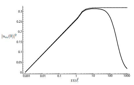
Figure 1: The graviton mode functions evaluated on the brane as a function of Kaluza-Klein mass $m$. The solid line is the function including the GB term, and the doted line is the one without GB term. The adopted parameter is $\chi=0.004$.

From eqs. (17), (23), (25), (26) and (27) we find that

$$\psi\simeq\frac{\kappa^{2}A\left(1-\gamma\right)}{2^{9}\pi^{3}}\sum_{n=1}^{\infty}\frac{2nT^{8}}{1+n}\times~{}~{}~{}~{}~{}~{}~{}~{}~{}~{}~{}~{}~{}~{}~{}~{}~{}~{}~{}~{}~{}~{}~{}~{}~{}$$

$$\int dx\frac{x^{6}K_{2}\left(\frac{1+n}{2}x\right)}{\pi\left(1+3\chi+\frac{15}{8}\chi^{2}+\chi^{2}\ell^{2}T^{2}x^{2}\right)}~{}~{}$$

$$\sim\left\{\begin{array}[]{c}\frac{\alpha_{GB}(1-\gamma)\kappa^{2}\rho^{3/2}}{\chi^{2}\ell^{2}}~{}~{}~{}~{}~{}~{}~{}\textmd{for}~{}m\sim T\gg 1/\chi\ell\\ \frac{\alpha_{RS}(1-\gamma)\kappa^{2}\rho^{2}}{1+3\chi+\frac{15}{8}\chi^{2}}~{}\textmd{for}~{}\ell^{-1}\ll m\sim T\ll 1/\chi\ell\end{array},\right.$$ (30)

where $K_{2}$ is the modified Bessel function of the second kind, and $\alpha_{GB,RS}$ is a dimensionless constant related to the total number of relativistic degrees of freedom. If all degrees of freedom of the standard model are relativistic, $\alpha_{GB}\simeq 4.56\times 10^{-4}$ and $\alpha_{RS}\simeq 1.54\times 10^{-3}$. We find that $\psi$ is proportional to $\rho^{3/2}$, not $\rho^{2}$ as in the RS case at high energy scales GBVaidya . Note that the transition energy scale depends on the bulk curvature scale $\ell$ and that this energy scale is lower than the RS energy scale for a wide range of values of $\ell$ and $\alpha$.

IV Numerical analysis

It is useful to define the dimensionless parameters, $\hat{\rho}=\rho/\lambda$, $\hat{t}=t/\ell$, $\hat{H}=H/\ell$, $\hat{C}=C/\ell^{2}$, and $\hat{\alpha}=\alpha/\ell^{2}$. The first four variables are the same as those used in Refs. RSrad1 ; RSrad2 . Using these variables, the dynamics on the brane are governed by the following system of differential equations:

$$\frac{d\hat{\rho}}{d\hat{t}}+4\hat{H}\hat{\rho}=-\hat{\psi},~{}~{}~{}~{}~{}~{}~{}~{}~{}~{}~{}~{}~{}~{}~{}~{}~{}~{}~{}~{}~{}~{}~{}~{}$$ (31)

$$\frac{d\hat{C}}{d\hat{t}}=\frac{2}{3}(3-\gamma)\hat{\psi}r^{4}\left(\sqrt{\hat{H}^{2}+\frac{1-b^{1/3}}{4\hat{\alpha}}}-\hat{H}\right),~{}~{}~{}~{}$$ (32)

$$\frac{d\hat{H}}{d\hat{t}}=-\hat{H}^{2}-\frac{1-b^{1/3}}{4\hat{\alpha}}-\frac{2\hat{C}}{r^{4}b^{1/3}}-\frac{(3-\gamma)\hat{\psi}}{3b^{1/3}}~{}~{}~{}~{}~{}$$

$$-\left\{2\left(b^{1/3}-\frac{8\hat{\alpha}\hat{C}}{r^{4}b^{1/3}}-\frac{\gamma(3-\gamma)\hat{\psi}}{3b^{1/3}}\right)\left(\hat{H}^{2}+\frac{1-b^{1/3}}{4\hat{\alpha}}\right)\right.$$

$$\left.+(1-\frac{\gamma}{3})\left(\hat{\rho}-3\right)\sqrt{\hat{H}^{2}+\frac{1-b^{1/3}}{4\hat{\alpha}}}\right\}$$

$$/\left\{1+8\hat{\alpha}\left(\hat{H}^{2}+\frac{1-b^{1/3}}{8\hat{\alpha}}\right)\right\},~{}~{}$$ (33)

where

$$\hat{\psi}=\frac{2\ell}{\lambda}\psi~{}~{}~{}~{}~{}~{}~{}~{}~{}~{}~{}~{}~{}~{}~{}~{}~{}~{}~{}~{}~{}~{}~{}~{}~{}~{}~{}~{}~{}~{}~{}~{}~{}~{}~{}~{}~{}~{}~{}~{}~{}~{}~{}~{}~{}~{}~{}~{}~{}~{}~{}~{}~{}~{}~{}~{}~{}~{}~{}~{}~{}$$

$$\sim\left\{\begin{array}[]{c}2\alpha_{GB}(1-\gamma)\sqrt{\frac{2(3-\gamma)}{1+\gamma}}\left(\frac{\kappa_{4}}{\ell}\right)\frac{\hat{\rho}^{3/2}}{\chi^{2}}~{}~{}\textmd{for}~{}T^{2}\gg 1/\chi^{2}\ell^{2}\\ \frac{4\alpha_{RS}(3-\gamma)(1-\gamma)\hat{\rho}^{2}}{1+3\chi+\frac{15}{8}\chi^{2}}~{}~{}~{}~{}\textmd{for}~{}\ell^{-2}\ll T^{2}\ll 1/\chi^{2}\ell^{2}{}{}{}{}{}{}{}{}\end{array}.\right.$$ (36)

In order to derive above equations we use eqs. (7), (14), (15), (16), (17) and (28). Unfortunately, it is very difficult to find a general analytic solution to these equations, such as that found by Leeper et. al. for the RS case RSradsolution . So, we use the approximation of eq. (32) and solve the above coupled system numerically. Here, the algebraic constraint from the generalized Friedmann equation,

$$\hat{H}^{2}=\frac{\hat{c}_{+}+\hat{c}_{-}-2}{8\hat{\alpha}},~{}~{}~{}~{}~{}~{}~{}~{}~{}$$

$$c_{\pm}=\left\{\left[b+2(3-\gamma)^{2}\hat{\alpha}\left(1+\hat{\rho}\right)^{2}\right.\right.$$

$$\left.\left.\pm\sqrt{2\hat{\alpha}}(3-\gamma)(1+\hat{\rho})\right]\right\}^{2/3}$$ (37)

is used to monitor numerical errors. Results from a numerical integration of this system with a variety of initial conditions for $\alpha$ and $\ell$ are shown in Figures 2-5. The initial value of $\hat{\rho}_{i}$ is taken $10^{4}$ except that $10^{4}$ is larger than the highest energy density scale $M^{4}/\lambda$ . In such cases we take $\hat{\rho}_{i}=M^{4}/\lambda$.

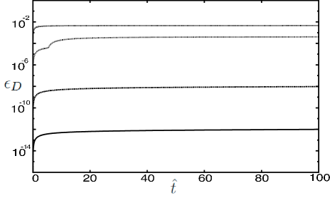
Figure 2: Evolution of $\epsilon_{D}$ with $\ell=1\textmd{GeV}^{-1}$. The curves from top to bottom correspond to the cases $\hat{\alpha}=10^{-10},10^{-9},10^{-7}\textmd{and}~{}10^{-5}$. We can see that the transition between $\psi\propto\rho^{3/2}$ and $\psi\propto\rho^{2}$ occurs in the second curve from above.

Figure 2 shows the effect of increasing $\alpha$ while keeing $\ell$ fixed. Here, we define $\epsilon_{D}$ as the ratio of dark radiation to standard radiation energy density:

$$\epsilon_{D}\equiv\frac{9\hat{C}}{2(3-\gamma)^{2}r^{4}\hat{\rho}}.$$ (38)

The first thing to notice is that the larger $\alpha$ is the smaller $\epsilon_{D}$. This is because the interaction between brane matter and the bulk gravitons weakens due to the GB term as can be seen in Figure 1 and the brane emits less gravitons.
 The evolution of $\epsilon_{D}$ with $\hat{\alpha}=10^{-7}$ is shown in Figure 3. There is also a marked effect on $\epsilon_{D}$. The increase of $\ell$ leads to an extension of the $\psi\propto\rho^{3/2}$ regime and a suppression of graviton emission by eq. (28).

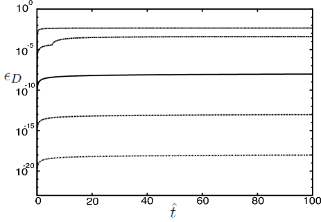
Figure 3: Evolution of $\epsilon_{D}$ with $\hat{\alpha}=10^{-7}$. The curves from top to bottom correspond to the cases $\ell=10^{-7},10^{-5},1,10^{-5},\textmd{and}~{}10^{10}\textmd{GeV}^{-1}$. We can also see that the transition between $\psi\propto\rho^{3/2}$ and $\psi\propto\rho^{2}$ occurs in the second curve from above.

At low energies, dark radiation is produced at a negligible rate so that there is an asymptotic constant value for $\epsilon_{D}$ as shown in Figures 2 and 3. These asymptotic values of $\epsilon_{D}$ are shown in Figures 4 and 5. We find that there is an upper bound on $\epsilon_{D}$ and that this upper bound value is the final value of the RS case RSrad1 :

$$\epsilon_{D}^{GB}<\epsilon_{D}^{RS}\rightarrow 3\alpha_{RS}.$$ (39)

This quantity is constrained by cosmological observations. The number of additional relativistic degrees of freedom is usually measured in units of extra neutrino species $\Delta N_{\nu}$. A typical bound $\Delta N_{\nu}\hskip 3.00003pt\raisebox{1.72218pt}{$<$}\raisebox{-3.01385pt}{$\sim$}\hskip 3.00003pt1$ extranu implies $\epsilon_{D}\hskip 3.00003pt\raisebox{1.72218pt}{$<$}\raisebox{-3.01385pt}{$\sim$}\hskip 3.00003pt0.35$. This bounds is just above the estimated value for the RS case. Including the GB term can help reduce the final value of the dark radiation term and hence we can easily satisfy this bound.

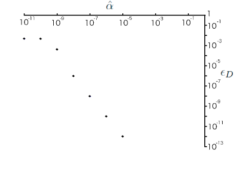
Figure 4: The asymptotic values of $\epsilon_{D}$ with $\ell=1\textmd{GeV}^{-1}$.

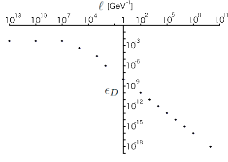
Figure 5: The asymptotic values of $\epsilon_{D}$ with $\hat{\alpha}=10^{-7}.$

V Conclusions

In this paper, we have considered a GB brane that emits gravitons at early times, using a generalized Ads-Vaidya spacetime approximation. We have derived the dynamical equations governing the evolution of the energy density $\rho$, the scale factor $r$, and the dark radiation parameter $C$ in section II. In section III we have derived the production rate of bulk gravitons.
 We have performed numerical integration of the system of differential equations in section IV. The different feature from a RS radiating brane is that the asymptotic value for the dark radiation depends on the curvature scale $\ell$ and the GB coupling term $\alpha$. And we have demonstrated that the late-time dark radiation is generally suppressed and so cosmological limits can be easily satisfied when there is a GB term.

- (1) L. Randall and R. Sundrum, Phys. Rev. Lett. 83, 4690 (1999).
- (2) A. Fayyazuddin and M. Spalinski, Nucl. Phys. B535, 219 (1998);O. Aharony, A. Fayyazuddin and J. Maldacena, JHEP 07 013 (1998).
- (3) D. Lovelock, J. Math. Phys. 12, 498 (1971).
- (4) C. Lanczos Ann. Math. 39, 842 (1938).
- (5) D. G. Boulware and S, Deser, Phys. Rev. Lett. 55, 2656 (1985); D. Wiltshire, Phys. Rev. D38 2445 (1988); J. Wheeler, Nucl. Phys. B268, 737 (1986); J. Crisostomo, R. Troncoso and J. Zanelli, Phys. Rev. D62 084013 (2000); A. Barrau, J. Grain, S. O. Alexeyev, Phys. Lett. B584 114 (2004); R. Konoplya, Phys. Rev. D71 024038 (2005); E. Abdalla, R. A. Konoplya, and C. Molina, Phys. Rev. D72 084006 (2005); F. Moura and R. Schiappa, Class. Quant. Grav. 24 361 (2007).
- (6) N.E. Mavromatos and J. Rizos, Phys. Rev. D 62,124004 (2000); I.P. Neupane, JHEP 09, 040 (2000); Phys. Lett. B 512, 137 (2001); K.A. Meissner and M. Olechowski, Phys. Rev. Lett. 86, 3708 (2001); Y.M. Cho, I. Neupane, and P.S. Wesson, Nucl. Phys. B621, 388 (2002).
- (7) N. Deruelle and M. Sasaki, Prog. Theor. Phys. 110, 441 (2003).
- (8) P. Binetruy, C. Deffayet, and D. Langlois, Nucl. Phys. B565 269 (2000); R. Maartens, Living Rev.Rel. 7 7 (2004); D. Langlois, Prog. Theor. Phys. Suppl. 148 181 (2003); P. Brax and C. van de Bruck, Class. Quant. Grav. 20 R201 (2003); G. Kofinas, R. Marartens, and E. Papantonopoulos, JHEP 10 066 (2003); J. P. Gregory and A. Padilla, Class. Quant. Grav. 20 4221 (2003); S. Nojiri and S. D. Odintsov, JHEP 07 049 (2000); S. Nojiri, S. D. Odintsov and S. Ogushi, Phys. Rev. D65 023521 (2001); S. Nojiri, S. D. Odintsov and S. Ogushi, Int. J. Mod. Phys. A17 4809 (2002); J. E. Lidsey, S. Nojiri and S. D. Odintsov, JHEP 06 026 (2002). N. Deruelle, and T. Dolezel, Phys. Rev. D62 103502 (2000); P. Bowcock,C. Charmousis, and R. Gregory, Class. Quant. Grav. 17 4745 (2000); B. Carter and J.-P. Uzan, Nucl. Phys. B606 45 (2001); R. A.Battye and B. Carter, Phys. Lett. B509 331 (2001); R. A.Battye, B. Carter, A. Mennim, and J.-P. Uzan, Phys. Rev. D64 124007 (2001); B. Carter, J.-P. Uzan, R. A.Battye, and A. Mennim, Class. Quant. Grav. 18 4871 (2001); A. Melfo, N. Pantoja, and A. Skirzewski, Phys. Rev. D67 105003 (2003); L. A. Gergely, Phys. Rev. D68 124011 (2003); O. Castillo-Felisola, A. Melfo, N. Pantoja, and A. Ramirez, Phys. Rev. D70 104029 (2004); A. Padilla, Quant. Grav. 22 681 (2005). A.-C. Davis, S. C. Davis, W. B. Perkins, and I. R. Vernon, Phys. Lett. B504 254 (2001); D. Ida, JHEP 09 014 (2000); P. S. Apostolopoulos, and N. Tetradis, Phys. Rev. D71 043506 (2005); P. S. Apostolopoulos, N. Brouzakis, E. N. Saridakis, and N. Tetradis, Phys. Rev. D72 044013 (2005); P. S. Apostolopoulos, and N. Tetradis, Phys. Lett. B633 409 (2006); N. Tetradis, Class. Quant. Grav. 21 5221 (2004); K. Konya, gr-qc/0605119.
- (9) D. Langlois, L. Sorbo, and M. Rodriguez, Phys. Rev. Lett. 89 17101 (2002);
- (10) A. Hebecker and J. March-Russell, Nucl. Phys. B608 375 (2001); L. Gergely, E. Leeper, and R. Maartens, Phys. Rev. D70 104025 (2004); E. Kiritsis, N. Tetradis, and T. N. Tomaras, JHEP 03 019 (2002); D. Langlois and L. Sorbo, Phys. Rev. D68 084006 (2003); I. R. Vernon and D. Jennings, JCAP 07 011 (2005); L. Gergely and Z. Keresztes, JCAP 01 022 (2006).
- (11) E. Leeper, R. Maartens, and C. Sopuerta, Class. Quant. Grav. 21 1125 (2004);
- (12) C. Charmousis, S. C. Davis, and J. Dufaux, Class. Quant. Grav. 19 4671 (2002).
- (13) D. G. Boulware and S. Deser, Phys. Rev. Lett. 55 2656 (1985); R.-G. Cai, Phys. Rev. D65 084014 (2002).
- (14) T. Kobayashi, Gen. Rel. Grav. 37 1869 (2005); H. Maeda, Class. Quant. Grav. 23 2155 (2006).
- (15) W. Israel, Nuovo Cimento Soc. Ital. Fis. B44 1 (1966); S. C. Davis, Phys. Rev. D67 024030 (2003); S. Willson, Phys. Lett. B562 118 (2003); K. Maeda and T. Torii, Phys. Rev. D69 024002 (2004);
- (16) J.-F. Dufaux, J. E. Lidsey, R. Maartens, and M. Sami, Phys. Rev. D70 083525 (2004).
- (17) I. P. Neupane, Phys. Lett. B512 137 (2001).
- (18) G. F. Giudice, R. Rattazzi, and J. D. Wells, Nucl. Phys. B544 3 (1999); T. Han, J. D. Lykken, and R. J. Zhang, Phys. Rev. D59 105006 (1999).
- (19) R. H. Cyburt, B. D. Fields, K. A. Olive and E. Skillman, Astropart. Phys. 23 313 (2005): V. Barger, J. P. Kneller, H. S. Lee, D. Marfatia and G. Steigman, Phys. Lett. B566 8 (2003): J. P. Kneller, R. J. Scherrer, G. Steigman and T. P. Walker, Phys. Rev. D64 123506 (2001).