Metastability of $R$-Charged Black Holes

Abstract

The global stability of $R$-charged AdS black holes in a grand canonical ensemble is examined by eliminating the constraints from the action, but without solving the equations of motion, thereby constructing the reduced action of the system. The metastability of the system is found to set in at a critical value of the chemical potential which is conjugate to the $R$-charge. The relation among the small black hole, large black hole and the instability is discussed. The result is consistent with the metastability found in the AdS/CFT-conjectured dual field theory. The “renormalized” temperature of AdS black holes, which has been rather ad hoc, is suggested to be the boundary temperature in the sense of AdS/CFT correspondence. As a byproduct of the analysis, we find a more general solution of the theory and its properties are briefly discussed.

1 Introduction

The global structure of a black hole action is the interest of this paper. Examination of this, in general, is a formidable task and the difficulties include the large number of the fields involved and the complicated nature of the action itself. For instance, in a single scalar theory at classical level, one simply plots the potential of the theory with respect to the expectation value of the scalar field and examines the global minimum of the theory. Similar program for a theory that involves gravity is not as straightforward due to the complications. Therefore, a black hole action is commonly studied by evaluating the values of it on known black hole solutions, by this means constructing the on-shell action of the theory. The on-shell action is valid in an infinitesimal neighborhood of the black hole saddle point and the local behavior of black holes, such as the first law of thermodynamics and local thermodynamic stability, can be studied from the action. This method, however, is not adequate for examining the global structure of a black hole action.

In Reference [1], Braden et al. devised the technique that yields a simplified off-shell action, called “reduced action” of a black hole system. The procedure for constructing the reduced action is as follows. One starts with the action of a system and place it in a finite box. Then, restrict the analysis to a class of geometries that satisfy certain conditions, such as static spherical symmetry. The restriction results in a specific form of the metric and this is analogous to a metric ansatz that one makes in solving the Einstein equation. In addition to the geometrical restriction, one imposes the black hole “cigar” topology on the spacetime manifold, giving a condition that the metric must satisfy. Next, the thermodynamic data is encoded on the wall of the box. The data, in the case of a grand canonical ensemble, is the temperature and chemical potential. (We will show exactly how to encode the data in Section 3.2). As will be explained in Section 3.3, the physical states of the system in general obeys constraint equations including the Hamiltonian constraint, and they are solved and eliminated from the action. Finally, the action functional is integrated with the topology condition and the boundary data, resulting in the simplified reduced action. Notice that the equations of motion have not been used in reducing the action. Thus the reduced action is valid throughout the physical parameter space and a black hole solution corresponds to a saddle point of the action in the parameter space. Therefore, this action captures the global structure of the theory.

After reviewing the five dimensional $R$-charged black hole solution and its properties in Section 2, in Section 3, we apply the procedure sketched in the previous paragraph to this black hole system in a grand canonical ensemble. This black hole system can be obtained through $S^{5}$ compactification of ten dimensional Type IIB supergravity with gauged $SO(6)$ global symmetry [2, 3]. A special case with decoupled scalars can be obtained rather simply by “twisting” the five sphere upon the compactification, as demonstrated by Chamblin et al. in Reference [4]. It has also been shown by Cvetič and Gubser in Reference [5] that the black hole geometry arises from the near horizon limit of rotating D3-branes in ten dimensions with the rotation in their transverse directions. Therefore this system has drawn numerous interests in connection to string theory and the examination of the global structure is worthwhile in its own right. However, there is an additional and more specific motivation for studying the global stability of the theory.

According to the AdS/CFT correspondence [6, 7, 8], the $R$-charged black hole system in a grand canonical ensemble is conjectured to be the dual of strongly coupled thermal $\mathcal{N}=4$ supersymmetric Yang-Mills theory in the large $N_{c}$ limit with the chemical potentials corresponding to the maximal Abelian subgroup of the $SU(4)$ $R$-summery. The weak coupling analysis of the field theory in Reference [9] shows that, despite the difference in the coupling regime, the phase diagram in the parameter space of temperature and chemical potential closely resembles the one obtained in the gravity analysis of Reference [5]. However, in the phase diagram of the field theory, the additional structure has been found where the equilibrium state of the system becomes metastable beyond a certain critical value of the chemical potential.

The metastability in the field theory was found by examining the global behavior of the scalar field effective potential at one-loop level. When the system is in the deconfined plasma phase with a sufficiently low value of the chemical potential, the origin of the scalar field space is the absolute minimum of the (one-loop) effective potential and defines the stable ground state of the theory. When the chemical potential is raised beyond the critical value, the effective potential goes down to minus infinity at the asymptotic region of the scalar expectation value. The minimum at the origin persists to exist in this phase but it now only is a local minimum with a potential barrier separating it from the unstable direction. The state at the origin, therefore, is metastable in this phase and the true ground state of the theory does not exist. Further rise in the chemical potential would eventually lead to the local instability of the state where the barrier that separates the local minimum and the unstable direction disappears.

We suspect that the metastability is caused by the violation of the BPS inequality expected for the states of the field theory. The chiral primary fields of $\mathcal{N}=4$ super-Yang-Mills theory contain the half-BPS operators that are characterized by their scaling dimension equaling their $R$-charges and in general, the dimension of an operator must be larger than or equal to the charge. When the theory is conformally mapped to a sphere, the operator and the dimension are mapped to a state of the theory and the energy of the state, respectively. Therefore, the half-BPS states have the energy being equal to the $R$-charges. When we introduce the chemical potential conjugate to the charge, we expect that the product of the charge and the chemical potential contributes to the total energy of the state. (Such an argument has been made in Reference [10] and further generalized in [11].) Hence if the chemical potential is raised higher than one (in the units of the radius of the sphere), we expect that the BPS inequality is violated and something should go wrong with the theory. The metastability of the field theory analysis sets in exactly at this critical value of the chemical potential.

Since the dimension of the BPS operator is protected against the quantum corrections and change in the coupling constant, we expect similar behavior in the gravitational analysis which is supposed to be the strong coupling region of the same theory. But it is clear that the local on-shell analysis that has been carried out in Reference [5] is not able to detect the metastability of the black hole system. This is why we embark on the program outlined above. Analyzing the resulting reduced action, we will find the metastability in Section 4.

In Section 5, a few issues that come up during the analysis are discussed. First in Section 5.1, the mysterious “renormalized” temperature that has been adopted in literature on the AdS black hole systems is suggested to be naturally understood in the context of the AdS/CFT correspondence. Then Section 5.2 presents a more general solution of the theory than what has been known. This solution is obtained as a byproduct of the main analysis and its properties are briefly discussed. Section 5.3 addresses a subtle issue of the physical interpretation of the counterterm that does not diverge as the wall of the box is pushed to infinity. Finally in Section 5.4, we contrast the revised phase diagram of the gravity side to the one in the field theory side.

2 Review of $R$-Charged Black Holes

We start by reviewing the $R$-charged black hole solution and their thermodynamics, mainly following Behrndt et al. [12] and Cvetič and Gubser [5]. The analysis on the instability of the black holes is slightly extended from the work of Cvetič and Gubser [5] for the cases with different charge configurations.

The $R$-charged black hole of our interest is the solution to five dimensional $\mathcal{N}=8$ gauged supergravity where the gauged symmetry is the $U(1)^{3}$ truncation of the $SO(6)$ global symmetry that arises from the $S^{5}$ compactification of ten dimensional supergravity. The solution is given by the metric

$$ds^{2}=-H(r)^{-2/3}f(r)dt^{2}+H(r)^{1/3}\big{[}f(r)^{-1}dr^{2}+r^{2}d\Omega_{3}^{2}\big{]}\;,$$ (1)

where $d\Omega_{3}^{2}$ is a metric on the unit three sphere and the function $H(r)$ is

$$H(r)=H_{1}(r)H_{2}(r)H_{3}(r)\quad\text{with}\quad H_{j}(r)=1+\frac{q_{j}}{r^{2}}\;,$$ (2)

and

$$f(r)=1-\frac{r_{0}^{2}}{r^{2}}+\frac{r^{2}}{R^{2}}H(r)\;.$$ (3)

The physical interpretations of the parameters $q_{j}$, $r_{0}$ and $R$ are as follows. As mentioned in the introduction, it is possible to interpret this solution as the near horizon limit of rotating D3-branes in ten dimensions and in this perspective, the parameters $q_{j}$ with the dimension length squared are related to the three possible transverse angular momenta of the D3-branes. (See Reference [5].) The parameter $r_{0}$ in the function $f$ measures the “non-extremality” of the black hole in that $r_{0}=0$ corresponds to the extremal BPS-saturated solution. The non-extremality parameter can be expressed in terms of the horizon radius $r_{H}$ by solving the equation $f(r_{H})=0$, explicitly,

$$r_{0}^{2}=r_{H}^{2}\bigg{\{}1+\frac{r_{H}^{2}}{R^{2}}H(r_{H})\bigg{\}}\;.$$ (4)

The parameter $R$ is the length scale of the theory. Note that the solution approaches to the AdS metric at the $r\to\infty$ asymptotic region and we see that the parameter $R$ is the curvature radius of this asymptotic AdS space. Therefore, it is also related to the cosmological constant.

This theory contains scalar fields, $X_{j}(r)$ with $j=1,\cdots,3$, satisfying the constraint

$$X_{1}(r)X_{2}(r)X_{3}(r)\equiv 1\;.$$ (5)

The solutions to the scalar fields are

$$X_{j}(r)=H_{j}(r)^{-1}H(r)^{1/3}\;.$$ (6)

This theory contains three dimensionless Abelian gauge fields arising from the gauged $U(1)^{3}$ and the solution takes the form

$$A_{j\,\nu}(r)=\delta_{\nu,0}\bigg{(}\frac{e_{j}}{r_{H}^{2}+q_{j}}-\frac{e_{j}}{r^{2}+q_{j}}\bigg{)}\;,$$ (7)

where $\nu$ is a spacetime index, the parameters $e_{j}$ with the dimension length squared are the electric charges of the system under the Abelian fields, the index $j$ runs, again, from $1$ to $3$ and we have set $A_{j\,\nu}(r_{H})=0$ for the reference point of the potentials. Observe that the time-component of the gauge fields at the coordinate $r$ is the electric voltage between the horizon and the location $r$. We denote the potentials at the boundary with $r=\infty$ by $\mu_{j}$ and they are

$$\mu_{j}=\frac{1}{R}\,\frac{e_{j}}{r_{H}^{2}+q_{j}}\;,$$ (8)

where the length scale $R$ is inserted for the dimensional reason. The parameters $q_{j}$ and $e_{j}$ are related through

$$e_{j}^{2}=q_{j}(r_{H}^{2}+q_{j})\bigg{[}1+\frac{r_{H}^{2}}{R^{2}}\prod_{k\neq j}H_{k}(r_{H})\bigg{]}\;,$$ (9)

where the repeated index $j$ is not summed over.

The ADM mass $M$ of the black hole is

$$M=\frac{\omega_{3}}{8\pi G_{5}}\bigg{(}\frac{3}{2}r_{0}^{2}+\sum_{j=1}^{3}q_{j}\bigg{)}\;,$$ (10)

where $\omega_{3}=2\pi^{2}$ is the volume of the unit three sphere and $G_{5}$ is the five dimensional Newton’s constant which has the dimension of length cubed. This ADM mass assumes the AdS background without the presence of the black hole, i.e., the mass $M$ is the mass difference between the AdS black hole spacetime and the thermal AdS space without the black hole. The entropy $S$ is a quarter of the horizon area as usual:

$$S=\frac{A}{4G_{5}}=\frac{2\pi^{2}r_{H}^{3}\sqrt{H(r_{H})}}{4G_{5}}\;.$$ (11)

The inverse Hawking temperature $\beta_{H}$ is given by the expression

$$\beta_{H}=\frac{2\pi R^{2}r_{H}^{5}\sqrt{H(r_{H})}}{2r_{H}^{6}+r_{H}^{4}(R^{2}+\sum_{j=1}^{3}q_{j})-\prod_{j=1}^{3}q_{j}}\;.$$ (12)

In Reference [5], the thermodynamic properties of the black hole in the grand canonical ensemble is examined by introducing the Gibbs free energy

$$I_{\text{Gibbs}}=\beta_{H}\bigg{(}M-\sum_{j=1}^{3}e_{j}\mu_{j}\bigg{)}-S\;,$$ (13)

where the length scale $R$ is set to $1$. The parameters $\beta_{H}$ and $\mu_{j}$ are the fixed data of the ensemble and the black hole corresponds to the saddle point of this function. Notice that the potentials $\mu_{j}$ are taken to be the chemical potentials of the grand canonical ensemble.

As mentioned earlier, the ADM mass is the difference between the black hole spacetime and the thermal AdS space without black holes. Thus, a change in the sign of the Gibbs free energy indicates that the ground state (or thermal equilibrium state) of the system switches from the black hole to the thermal AdS or vice versa. This is the well-known Hawking-Page phase transition [16]. The phase transition line of the phase diagram in $(\mu,T)$ parameter space can therefore be determined by the condition $I_{\text{Gibbs}}=0$.

Cvetič and Gubser [5] further examined the local thermodynamic stability of the black hole solutions. At an instability point, the black hole solution that extremizes the Gibbs free energy becomes an unstable saddle point, as opposed to a local minimum. Therefore, when the Hessian of $I_{\text{Gibbs}}$ with respect to $r_{H}$ and $q_{j}$ is evaluated at the black hole solution, the determinant of the Hessian vanishes at the critical local instability point. This condition establishes the instability line in the phase diagram. Even though this criterion does not determine which side of the instability line corresponds to the stable black hole, one can figure that by knowing that the region of high temperature and zero chemical potential must correspond to a stable black hole solution.

Figure 1: The phase diagram on the left is plotted for $(q_{1},q_{2},q_{3})=(q,0,0)$ and on the right is for $(q,q,q)$. Both $\mu$ and $T$ are measured in the units of $1/R$, the inverse of the AdS curvature radius. The solid and dotted lines are the black hole instability lines whereas the dashed lines are the Hawking-Page phase transition lines. The regions between the dashed and dotted lines indicate the spinodal phases where the AdS space is energetically preferred but the black hole still remains locally stable. The temperature $T_{0}=1/\pi$ on the left-hand diagram is where $r_{H}=0$.

The resulting phase diagrams are plotted in Figure 1. We choose to plot the phase diagram in $\mu$-$T$ plane as oppose to Reference [5] whose choice is $q$-$r_{H}$ plane. We have also extended the analysis of the same reference to the cases with more than one $q$ is turned on. The left-hand diagram is plotted for $(q_{1},q_{2},q_{3})=(q,0,0)$ and the right is for $(q,q,q)$. The solid and dotted lines are the black hole instability lines whereas the dashed lines are the Hawking-Page phase transition lines. The regions between the dashed and dotted lines indicate the spinodal phases where the AdS space is energetically preferred but the black hole still remains locally stable. The general structure of the phase diagrams are similar for the different charge configurations [including the case with $(q,q,0)$]. However the low temperature regions are quite different. The temperature $T_{0}$ in the left-hand diagram denotes the Hawking temperature at which $r_{H}=0$. When we have three equal non-zero charges, $T_{0}=0$, but for the case with the only one non-zero charge, $T_{0}\neq 0$. The exact values of the $T_{0}$ are listed in Table 1 for the different cases.

$(q_{1},q_{2},q_{3})$ $(q,0,0)$ $(q,q,0)$ $(q,q,q)$ $T_{0}$ $1/\pi$ $1/2\pi$ $0$ Asymp. Slope $\pi/\sqrt{2}$ $\pi$ $2\pi$

Table 1: The list of the values of $T_{0}$ and the slops of the high temperature linear behavior for different cases.

Since the action is the difference between the black hole and AdS solutions, the region of the phase diagram below $T_{0}$ is completely undetermined.

In all the cases, the instability lines and the Hawking-Phage phase transition lines merge at $T=T_{0}$ and $\mu=1/R$ where $R$ is the AdS curvature radius. The solid instability lines rise linearly at temperature large compared to $1/R$ and the slopes of the linear behavior is also listed in Table 1 for the different cases.

We mention that the instabilities of the black holes with $q_{1}=q_{2}$ and $q_{1}=q_{2}=q_{3}$ are obtained by assuming that the equalities are subject to the thermal fluctuations around the black hole saddle points. Technically, this means that the Hessian of $I_{\text{Gibbs}}$ with respect to $q_{j}$ is computed by assuming they are the independent parameters, and then the Hessian is evaluated at the black hole saddle point with the relations $q_{1}=q_{2}$ or $q_{1}=q_{2}=q_{3}$. One may choose to consider the black hole with the constraint $q_{1}\equiv q_{2}$ or $q_{1}\equiv q_{2}\equiv q_{3}$ which is not subject to the fluctuations. In this case, the action $I_{\text{Gibbs}}$ is obtained by setting $q_{1}\equiv q_{2}$ or $q_{1}\equiv q_{2}\equiv q_{3}$ first, and then the Hessian is computed with respect to the single charge (and $r_{H}$). The resulting thermodynamic system for this constrained case is stable everywhere and the instability lines are not observed. The constraints reduce the dimension of the parameter space and eliminate the direction of the instabilities. This is the reason why the instability found in Reference [5] [with the configuration $(q,0,0)$] is not observed in the analysis of Reference [4] [with the configuration $(q,q,q)$].

In concluding the review, we point out that the Gibbs free energy $I_{\text{Gibbs}}$ is constructed out of the quantities of the black hole. The black hole is the solution of the equations of motion and thus $I_{\text{Gibbs}}$ is made out of the on-shell quantities. Therefore, even though we expect the Gibbs free energy to be the action of the theory in an infinitesimal neighborhood of the black hole extremum, we have no guarantee that $I_{\text{Gibbs}}$ has any meaning as the action of the theory away from the extremum. The function $I_{\text{Gibbs}}$ is a local on-shell action in this sense and it is not useful in examining the global stability of the theory. The examination of the global stability requires the construction of the off-shell action that is valid away from the extremum.

3 Construction

3.1 The Action, the Metric, and the Topology

We now embark on constructing the reduced action of the system. In this subsection, we first display the action and the metric ansatz to start. Then we assume the Euclidean black hole topology on spacetime and deduce the resulting conditions on the metric.

As shown in Reference [12], the black hole solution reviewed in the previous section can be obtained from the following special case of the five dimensional $\mathcal{N}=2$ gauged supergravity action

$$I=-\frac{1}{8\pi G_{5}}\int d^{5}x\sqrt{g}\bigg{[}\frac{1}{2}\mathcal{R}-\frac{1}{2}\sum_{j=1}^{3}\frac{1}{2X_{j}^{2}}(\partial_{\mu}X_{j})(\partial^{\mu}X_{j})-\frac{1}{4}\sum_{j=1}^{3}\frac{1}{2X_{j}^{2}}F_{j\,\mu\nu}{F_{j}}^{\mu\nu}+\frac{V}{R^{2}}\bigg{]}\;,$$ (14)

where only the bosonic sector is shown. We have adopted the Euclidean signature and the sign of the action is chosen so that the weight factor in the path integral appears as $\exp(-I)$. The Chern-Simons term is dropped from the action because we will be considering the electrostatic fields which have the form $A_{j\,\nu}=A_{j\,\tau}\delta_{\nu,0}$, and the term identically vanishes for such fields. The determinant of the metric is denoted by $g$, and $\mathcal{R}$ is the scalar curvature. As in the previous section, the fields $X_{j}(x)$ are the scalars and they satisfy the constraint

$$X_{1}(x)X_{2}(x)X_{3}(x)\equiv 1\;.$$ (15)

The three gauged $U(1)^{3}\subset SO(6)$ Abelian fields $A_{j\,\nu}$ have the corresponding field strengths

$$F_{j\,\mu\nu}:=A_{j\,\nu;\mu}-A_{j\,\mu;\nu}\;,$$ (16)

where the indices $\mu$ and $\nu$ are the spacetime indices and the semicolon denotes the geometrical covariant derivative with respect to a given metric, which, of course, can be replaced by normal derivatives in this case. The potential $V$ is defined as

$$V:=2\sum_{j=1}^{3}\frac{1}{X_{j}}\;.$$ (17)

Finally in the action, the parameter $R$ is the length scale of the theory which is related to the cosmological constant of the asymptotic geometry.

We consider the static gravitational system with spherical symmetry and thus take the metric ansatz

$$ds^{2}=b(r)^{2}d\tau^{2}+H(r)^{1/3}\big{[}f(r)^{-1}dr^{2}+r^{2}d\Omega_{3}^{2}\big{]}\;,$$ (18)

where $\tau$ is the periodic Euclidean time whose period is set to $2\pi R$. Consequently, $b(r)$ is a dimensionless function of $r$. The form of the metric is completely general under the static spherical symmetry but we choose the particular form that resembles the solution of the previous section in Equation (1). This choice is motivated by the fact that we want the resulting reduced action to reproduce the same form of the solution as in the previous section at the extremum. Without loss of generality, we may assume that the dimensionless function $H(r)$ is positive definite and finite for finite values of $r$ so that the horizon in the Minkowski signature is determined solely by the dimensionless function $f(r)$. Notice that the static spherical symmetry requires the scalar fields $X_{j}(x)$ be functions only of $r$ as well.

In the computations that follow, we place the thermodynamic system into a large box whose wall is located at $r=r_{B}$ (the word “large” is used with respect to the length scale $R$). In the AdS/CFT language, this is the “cut-off boundary” of the system and will be removed by taking the limit $r_{B}\to\infty$. The lower end of the range of the parameter $r$ is given at $r=r_{H}$ which is the horizon radius of the black hole in the Minkowski signature. We will loosely use the terminology, “horizon radius”, even if we are discussing the Euclidean black holes.

In addition to the static spherical symmetry, we restrict our considerations to the action that describes the spacetimes with Euclidean black hole topology. The Euclidean black hole topology of the spacetime manifold is $\mathbb{R}^{2}\times S^{3}$ and the boundary of the manifold has the topology $S^{1}\times S^{3}$ where the $S^{1}$ factor corresponds to the periodic Euclidean time circle. In the actual computation, we assume the topology $S^{1}\times S^{3}$ at the wall of the box, $r=r_{B}$, with the limit $r_{B}\to\infty$ in our mind.

We first want to impose the topology $\mathbb{R}^{2}\times S^{3}$ on the entire spacetime. However, the Euler characteristic of any odd dimensional manifold identically vanishes and it is not desired here. Thus, we fix one of the angular coordinates in $S^{3}$ and require this slice to have the topology $\mathbb{R}^{2}\times S^{2}$ with the Euler characteristic $\chi$ equaling $2$. This yields the condition

$$\Big{[}fH^{-1/3}\big{\{}(rH^{-1/6})^{\prime}\big{\}}^{2}\Big{]}_{r=r_{H}}=0\;,$$ (19)

where the prime denotes the derivative with respect to the radial coordinate $r$ and the left-hand side of the equation is evaluated at $r=r_{H}$. We will see that this condition boils down to the expected condition for a black hole horizon, $f(r_{H})=0$.

Next, consider the $\mathbb{R}^{2}$ part of the spacetime. This is commonly called “the cigar” where the tip of the cigar corresponds to the black hole horizon and thus it is parametrized by the lower end of the radial coordinate $r=r_{H}$, whereas the other end of the cigar is the boundary $S^{1}$. In this topology, the $S^{1}$ time circle degenerates at the tip $r=r_{H}$ and thus we have

$$b(r_{H})=0\;.$$ (20)

Also this topology requires the $\tau$-$r$ slice of the spacetime to have the Euler characteristic $\chi=1$ as the cigar is topologically a two dimensional ball with boundary. This condition parallels with the usually known “smoothness condition” at the tip of the cigar. Being cautious for the orientation of the $S^{1}$ time circle at the wall of the box, the Gauss-Bonnet theorem yields

$$\left[b^{\prime}f^{1/2}H^{-1/6}\right]_{r=r_{H}}=1/R\;.$$ (21)

There are terms evaluated at $r=r_{B}$, one from the Gauss curvature part and the other from the geodesic curvature of the boundary curve, but they cancel and absent in the above expression.

3.2 The Boundary Data

We encode the boundary data of the system in this subsection. Those data will be the fixed parameters of the “histories” of the paths in the path integral and they will not be varied in the extremization of the action. Since we want to consider and fit the black hole system in the context of the AdS/CFT correspondence, we have the metric satisfy the asymptotic AdS geometry near the boundary. Also we are interested in the grand canonical ensemble of the black hole thermodynamics, so the temperature and chemical potentials are the fixed parameters. If there is a physically equivalent field theory on the boundary, then those fixed black hole thermodynamic data should be identical to the ones in the field theory. Therefore, it is natural to encode the fixed parameters on the boundary where the geometry is fixed and the corresponding field theory is supposed to live.

First, we want the asymptotic AdS geometry near the boundary. We impose the asymptotic conditions on the metric ansatz (18)

$$b(r_{B})\to\ell\frac{r_{B}}{R}\;,\quad f(r_{B})\to\frac{r_{B}^{2}}{R^{2}}\;,\quad H(r_{B})\to 1\;,\quad\text{as}\quad r_{B}\to\infty\;.$$ (22)

The parameter $\ell$ is an arbitrary dimensionless positive constant. The motivation for introducing the parameter $\ell$ shall be given shortly in the discussion of the temperature below. One sees that with the analytic continuation, $t=-i\ell\tau$, the metric ansatz (18) approaches to the AdS metric with the curvature radius $R$, up to the first order in $r_{B}$.

Next we discuss the temperature of the system. It is sometimes seen that an observer is not specified for the discussion of the black hole temperature. However, the inverse temperature is the circumference of the $S^{1}$ Euclidean time circle and it depends on the location of the observer. For our metric, the local, physical inverse temperature at $r=r_{B}$ is the proper length of the $S^{1}$ circumference

$$\tilde{\beta}=\int^{2\pi R}_{0}d\tau b(r_{B})=2\pi R\,b(r_{B})\;.$$ (23)

Due to the asymptotic AdS condition on $b(r)$ in (22), the physical temperature is red-shifted to zero as the wall is pushed to the boundary, i.e., as $r_{B}\to\infty$. This fact has been known since as early as Hawking and Page [16]. We could have discussed the thermodynamics defined in a finite box with $r_{B}<\infty$, but since we are interested in the AdS/CFT correspondence, we must take the limit $r_{B}\to\infty$.

In discussing the thermodynamics of AdS black holes in the infinite box, the unphysical temperature, so-called “renormalized temperature”, has been used. (Among the works that adopt the “renormalized” temperature, we refer to one paper [17] in which this issue is clearly addressed.) The “renormalized” temperature is defined by the product of the physical temperature at $r=r_{B}$ and the red-shift factor of the black hole geometry so that the limit $r_{B}\to\infty$ yields a finite value. (Consequently, if we set the boundary temperature to the finite value, the temperature diverges everywhere in the bulk). Even though the physical meaning of the redefined temperature has remained unclear, there have been indications that this, at least formally, is the correct temperature to be used on the boundary. The indications include the correct forms of the heat capacity, first law of thermodynamics and the quarter area law of the entropy, all with the redefined temperature [16, 17, 18]. In addition, our analysis below also requires a similar kind of redefinition in the temperature. Therefore, we introduce the new temperature $\beta$ defined at the boundary by

$$\beta:=\lim_{r_{B}\to\infty}\bigg{(}\frac{R}{r_{B}}\bigg{)}\tilde{\beta}=2\pi\ell R\;.$$ (24)

Here we see that the temperature is directly proportional to the arbitrary parameter $\ell$. Thus the temperature is a thermodynamic quantity that we can tune, not the system, as a grand canonical ensemble should be. We will discuss more on the redefined temperature in Section 5.1.

Finally, we encode the chemical potentials that are conjugate to the $R$-charges of the system. In a grand partition function, a chemical potential couples to the conjugate charge which is the time component of a conserved current. Therefore, the chemical potential is directly related to the time component of the gauge field that minimally couples to the conserved current. Thus we define the chemical potentials at the wall $r=r_{B}$ as

$$\tilde{\mu}_{j}:=\frac{1}{\tilde{\beta}}\ln\exp\bigg{[}i\oint A_{j}/R\bigg{]}\;,$$ (25)

where the integral on the right-hand side is defined on the $S^{1}$ time circle at $r=r_{B}$ and $A_{j}$ are the Hermitian gauge field one-forms. In the definition, the length scale $R$ is inserted for the dimensional reason. We choose the (Wick rotated) gauge field of the form

$$A_{j\,\nu}=A_{j\,\tau}(r)\delta_{\nu,0}\;.$$ (26)

This form assumes the electrostatic spherical symmetry. Then we have

$$\oint A_{j}=\oint(-i\ell A_{j\,t})(idt/\ell)=\oint A_{j\,\tau}d\tau=2\pi RA_{j\,\tau}(r_{B})\;,$$ (27)

where the analytic continuation $t=-i\ell\tau$ has been done and $A_{j\,\tau}$ now is pure imaginary. Therefore, we get

$$\tilde{\mu}_{j}=\frac{2\pi i}{\tilde{\beta}}A_{j\,\tau}(r_{B})\;.$$ (28)

Now if we assume that the gauge fields $A_{j\,\nu}(r_{B})$ are finite as $r_{B}\to\infty$, then the chemical potentials $\tilde{\mu}_{j}$ at the boundary vanish because $\tilde{\beta}$ diverges due to the asymptotic AdS condition (22). Thus, similar to the case of the temperature, we define the boundary chemical potentials by

$$\mu_{j}:=\lim_{r_{B}\to\infty}\bigg{(}\frac{r_{B}}{R}\bigg{)}\tilde{\mu}_{j}\;.$$ (29)

This definition will be discussed further in Section 5.1 along with the temperature $\beta$ defined in Equation (24).

We add that since we have the condition (20), we need to have the conditions

$$A_{j\,\tau}(r_{H})=0\;,$$ (30)

so that the proper local value of the gauge potential $A_{j\,\tau}(r_{H})/b(r_{H})$ can be set to zero as the reference point of the potential.

3.3 The Constraints

Our system has two sets of constraints; Gauss’ law and the Hamiltonian constraint. The physical states of the theory must satisfy the constraints and we treat them fixed and not subject to the variation. The way they arise is very similar. Among the Maxwell and Einstein equations, the constraints correspond to the non-dynamical equations, i.e., the ones without second order time derivatives. The constraints can also be viewed as the resulting equations of the variation with respect to Lagrange multipliers. In the electrodynamics, the Lagrange multiplier is the time component of the gauge field. In the ADM formalism [22, 19] of the geometrodynamics, the shift and lapse functions are the Lagrange multipliers. Below, we bring the action (14) to the form where the Lagrange multipliers explicitly appear and eliminate the constraints from the action, without imposing the dynamical equations of motion.

We first consider the gravitational part of the action (14),

$$I_{G}=-\frac{1}{8\pi G_{5}}\int d^{5}x\sqrt{g}\,\frac{1}{2}\mathcal{R}\;.$$ (31)

One can verify that with the metric of the form (18), the scalar curvature $\mathcal{R}$ can be written as

$$-\frac{1}{2}\mathcal{R}=\frac{f^{1/2}}{b\,r^{3}H^{2/3}}\big{(}b^{\prime}r^{3}f^{1/2}H^{1/3}\big{)}^{\prime}+{G^{\tau}}_{\tau}\;,$$ (32)

where the last term is the ${(^{\tau}}_{\tau})$-component of the Einstein tensor and it explicitly has the form

$${G^{\tau}}_{\tau}=\frac{3}{2r^{3}H^{1/2}(rH^{1/6})^{\prime}}\Big{[}r^{2}H^{1/3}\Big{(}fH^{-1/3}\big{\{}(rH^{1/6})^{\prime}\big{\}}^{2}-1\Big{)}\Big{]}^{\prime}\;.$$ (33)

Notice that this expression is independent of the function $b$. Now $I_{G}$ can be expressed as

$$I_{G}=\frac{\omega_{3}}{8\pi G_{5}}\,2\pi R\bigg{\{}\int dr\,(b^{\prime}r^{3}f^{1/2}H^{1/3})^{\prime}+\int dr\,b\,r^{3}f^{-1/2}H^{2/3}{G^{\tau}}_{\tau}\bigg{\}}\;.$$ (34)

To proceed further, we need to introduce the Gibbons-Hawking term [23] to the gravitational part of the action $I_{G}$. In general, the Gibbons-Hawking term is required so that a gravitational action has the consistent variational principle with respect to general variation of the metric whose induced metric on the wall of the box is held fixed. The Gibbons-Hawking term is not unique and one is allowed to include arbitrary term that depends only on the induced metric on the wall which can be immersed in a different spacetime. This arbitrary term is commonly used to set the reference background geometry of the action. However, the introduction of the background geometry is arbitrary and sometimes it is not possible to set a seemingly natural background. Thus, it is more desirable to construct our action independent of the background, therefore, we do not include the ambiguous term here and instead, adopt the AdS/CFT motivated background independent counterterms as discussed in the next subsection. The Gibbons-Hawking term without the subtraction term has the form

$$I_{GH}=\frac{1}{8\pi G_{5}}\int_{\partial M}d^{4}x\sqrt{\gamma}K\;,$$ (35)

where $\partial M$ is the wall at $r=r_{B}$ with the metric

$$ds_{4}^{2}=b(r_{B})^{2}d\tau^{2}+H(r_{B})^{1/3}r_{B}^{2}d\Omega_{3}^{2}\;,$$ (36)

and $\gamma$ is the determinant with respect to this metric. The factor $K$ is the trace of the extrinsic curvature

$$K_{\mu\nu}=-\frac{1}{2}\left(n_{\mu;\nu}+n_{\nu;\mu}\right)\;,$$ (37)

where $n_{\mu}$ is a normal unit vector of the wall, $\partial M$, and is given by

$$n_{\mu}=\Big{(}0,H^{1/6}/f^{1/2},0,0,0\Big{)}\;.$$ (38)

A straightforward computation yields

$$I_{GH}=-\frac{\omega_{3}}{8\pi G_{5}}2\pi R\Big{[}f^{1/2}H^{-1/6}\left(b\,r^{3}H^{1/2}\right)^{\prime}\Big{]}_{r=r_{B}}\;.$$ (39)

We combine Equations (34) and (39). After some algebra, we obtain

$$I_{G}+I_{GH}= -\frac{\omega_{3}}{8\pi G_{5}}\bigg{\{}\tilde{\beta}\,\Big{[}f^{1/2}H^{-1/6}(r^{3}H^{1/2})^{\prime}\Big{]}_{r=r_{B}}+2\pi r_{H}^{3}\sqrt{H(r_{H})}\bigg{\}}$$

$$+\frac{\omega_{3}}{8\pi G_{5}}\,2\pi R\int dr\,b\,r^{3}f^{-1/2}H^{2/3}{G^{\tau}}_{\tau}\;,$$ (40)

where the topological condition (21) and the definition of $\tilde{\beta}$ in (23) have been used.

We proceed to the Maxwell part of the action

$$I_{EM}=\frac{1}{8\pi G_{5}}\int d^{5}x\sqrt{g}\,\frac{1}{4}\sum_{j}\frac{1}{2X_{j}^{2}}\,F_{j\,\mu\nu}{F_{j}}^{\mu\nu}\;.$$ (41)

We define the Maxwell field tensors as in Equation (16) and with our metric (18) and the gauge fields (26), the only nonzero components are

$${F_{j\,01}}=-{F_{j\,10}}=-({A_{j\,\tau}})^{\prime}\;,$$ (42)

where the components with $\mu,\nu=1$ are the radial $r$-component. We introduce auxiliary fields $E_{j}(r)$ such that

$$I_{EM}=\frac{\omega_{3}}{8\pi G_{5}}\pi R\int dr\,b^{-1}r^{3}f^{1/2}H^{1/3}\sum_{j}\frac{1}{2X_{j}^{2}}(-E_{j}^{2}+2E_{j}F_{j\,10})\;.$$ (43)

Notice that $\delta I_{EM}/\delta E_{j}=0$ yields $E_{j}=F_{j\,10}$ and insertion of this equation back into $I_{EM}$ recovers the original form of the Maxwell action. For the factor $F_{j\,10}$ in the second term, we use the relation (42) and express that in terms of the derivative with respect to $r$ acting on $A_{j\,\tau}$. We then integrate this by parts to obtain

$$I_{EM}= -\frac{\omega_{3}}{8\pi G_{5}}\pi R\int dr\,b^{-1}r^{3}f^{1/2}H^{1/3}\sum_{j}\frac{1}{2X_{j}^{2}}E_{j}^{2}$$

$$-\frac{\omega_{3}}{8\pi G_{5}}2\pi R\int dr\sum_{j}\Big{(}b^{-1}r^{3}f^{1/2}H^{1/3}\frac{1}{2X_{j}^{2}}E_{j}\Big{)}^{\prime}A_{j\,\tau}$$

$$+\frac{\omega_{3}}{8\pi G_{5}}2\pi R\int dr\Big{(}b^{-1}r^{3}f^{1/2}H^{1/3}\sum_{j}\frac{1}{2X_{j}^{2}}E_{j}\,A_{j\,\tau}\Big{)}^{\prime}$$ (44)

We note that the last term is a total derivative and does not contribute to the equations of motion.

Finally, the scalar part of the action takes the form

$$I_{S}= -\frac{1}{8\pi G_{5}}\int d^{5}x\sqrt{g}\,\sum_{j}\bigg{[}-\frac{1}{4X_{j}^{2}}(\partial_{\mu}X_{j})(\partial^{\mu}X_{j})+\frac{2}{R^{2}}\frac{1}{X_{j}}\bigg{]}$$

$$= -\frac{\omega_{3}}{8\pi G_{5}}\,2\pi R\int dr\,b\,r^{3}f^{-1/2}H^{2/3}\sum_{j}\bigg{[}-fH^{-1/3}\,\frac{(X_{j}^{\prime})^{2}}{4X_{j}^{2}}+\frac{2}{R^{2}}\frac{1}{X_{j}}\bigg{]}\;.$$ (45)

Now in the total action

$$I=I_{G}+I_{GH}+I_{EM}+I_{S}\;,$$ (46)

we clearly see that $A_{j\,\tau}$ in $I_{EM}$ are the Lagrange multipliers. The variation with respect to those fields yields Gauss’ law constraint of the system,

$$\Big{(}b^{-1}r^{3}f^{1/2}H^{1/3}\frac{1}{2X_{j}^{2}}E_{j}\Big{)}^{\prime}=0\;,$$ (47)

where the repeated index $j$ is not summed over. We introduce the integration constants $-ie_{j}$ so that

$$E_{j}=-2i\,b\,f^{-1/2}H^{-1/3}X_{j}^{2}\;\frac{e_{j}}{r^{3}}\;.$$ (48)

The constants $e_{j}$ describe the real (as opposed to complex) charges that satisfy Gauss’ law and the factor of $-i$ is inserted to account for the analytic continuation from Minkowski to Euclidean space.

Using Equation (48), $I_{EM}$ can be expressed as

$$I_{EM}=\frac{\omega_{3}}{8\pi G_{5}}\bigg{\{}2\pi R\int dr\,b\,r^{-3}f^{-1/2}H^{-1/3}\sum_{j}e_{j}^{2}X_{j}^{2}-R^{3}\tilde{\beta}\sum_{j}\Big{(}\frac{e_{j}}{R^{2}}\Big{)}\tilde{\mu}_{j}\bigg{\}}\;,$$ (49)

where the last term comes from the evaluation of the total derivative term in Equation (3.3) and we have applied the boundary conditions (28) and (30).

The total action at this point has the form

$$I= -\frac{\omega_{3}R^{3}}{8\pi G_{5}}\bigg{\{}\frac{\tilde{\beta}}{R^{3}}\,\Big{[}f^{1/2}H^{-1/6}(r^{3}H^{1/2})^{\prime}\Big{]}_{r=r_{B}}+\tilde{\beta}\sum_{j}\Big{(}\frac{e_{j}}{R^{2}}\Big{)}\tilde{\mu}_{j}+2\pi\Big{(}\frac{r_{H}}{R}\Big{)}^{3}\sqrt{H(r_{H})}\bigg{\}}$$

$$+\frac{\omega_{3}}{8\pi G_{5}}\,2\pi\int dr\,b\,r^{3}f^{-1/2}H^{2/3}\Big{(}{G^{\tau}}_{\tau}-8\pi G_{5}{T^{\tau}}_{\tau}\Big{)}\;,$$ (50)

where ${T^{\tau}}_{\tau}$ is defined as

$${T^{\tau}}_{\tau}:=\frac{1}{8\pi G_{5}}\sum_{j}\bigg{[}-\frac{e_{j}^{2}\,X_{j}^{2}}{r^{6}H}-\frac{1}{4}\frac{f\,(X_{j}^{\prime})^{2}}{H^{1/3}X_{j}^{2}}+\frac{2}{R^{2}}\;\frac{1}{X_{j}}\bigg{]}\;.$$ (51)

We have noted that ${G^{\tau}}_{\tau}$ shown in (33) is free of the function $b$. Therefore, in the total action (3.3), we explicitly see that the function $b$ is the Lagrange multiplier that enforces the constraint

$${G^{\tau}}_{\tau}=8\pi G_{5}{T^{\tau}}_{\tau}\;.$$ (52)

One can verify that this, in fact, is the ${(^{\tau}}_{\tau})$-component of the Einstein equations and thus, this is the Hamiltonian constraint of the system.

Given the expressions (33) and (51), the Hamiltonian constraint (52) is a differential equation of functions $f$, $H$ and $X_{j}$ with respect to the variable $r$. We solve this differential equation by making ansatz which is similar to the one made in Reference [12],

$$f(r)=1-\frac{r_{0}^{2}}{r^{2}}+\frac{r^{2}}{R^{2}}H(r)\quad\text{and}\quad X_{j}(r)=H_{j}^{-1}H(r)^{1/3}\;,$$ (54)

where $r_{0}$ is an undetermined parameter and the functions $H_{j}$ are defined as $H_{j}:=1+q_{j}/r^{2}$. Now because of the constraint (15) imposed on the scalar fields, the function $H(r)$ is determined to be

$$H(r)=H_{1}(r)H_{2}(r)H_{3}(r)\;.$$ (55)

Thus we see that $q_{j}$ are the three parameters of the three fields; $H$ and $X_{j}$ with the constraint (15). Notice that this ansatz is consistent with the asymptotic condition (22). The form of the function $H$ above implies that the topology condition (19) is equivalent to the equation

$$f(r_{H})=0\;,$$ (56)

as advertised. Using this condition, we can trade the parameter $r_{0}$ of the function $f$ with the parameter $r_{H}$, just as in Equation (4). Then the Hamiltonian constraint (52) is satisfied if and only if

$$e_{j}^{2}=q_{j}(r_{H}^{2}+q_{j})\bigg{[}1+\frac{r_{H}^{2}}{R^{2}}\prod_{k\neq j}H_{k}(r_{H})\bigg{]}\;,$$ (57)

where the repeated index $j$ is not summed over. One observes that these relations are identical to the ones obtained in the on-shell analysis of Section 2 as shown in Equation (9).

In solving the Hamiltonian constraint, we have adopted the rather tight ansatz (54). This narrow assumption on the functions restrict the form of possible solutions. Instead of adopting the ansatz discussed above, we can assume the forms of the scalars $X_{j}$ and the function $H$ only, and regard the Hamiltonian constraint as a first order differential equation of the function $f(r)$. The solution to the differential equation generates a new family of solutions that includes the solution discussed in Section 2 as a special case. We will discuss this more general solution in Section 5.2.

3.4 The Boundary Reduced Action

In the previous subsection, we have solved and eliminated the constraints of the system. Thus the action now takes the form

$$I=-\frac{\omega_{3}R^{3}}{8\pi G_{5}}\bigg{\{}\frac{\tilde{\beta}}{R^{3}}\,\Big{[}f^{1/2}H^{-1/6}(r^{3}H^{1/2})^{\prime}\Big{]}_{r=r_{B}}+\tilde{\beta}\sum_{j}\Big{(}\frac{e_{j}}{R^{2}}\Big{)}\tilde{\mu}_{j}+2\pi\Big{(}\frac{r_{H}}{R}\Big{)}^{3}\sqrt{H(r_{H})}\bigg{\}}\;.$$ (58)

This action describes the thermodynamics of the black hole system in the box with the wall at $r=r_{B}$. As a grand canonical ensemble, the temperature $\tilde{\beta}$ and the chemical potentials $\tilde{\mu}_{j}$ are defined at the wall and the grand canonical data at other locations in the box cannot be deduced from $\tilde{\beta}$ and $\tilde{\mu}_{j}$, for the functions $b$ and $A_{j\,\tau}$ are the Lagrange multipliers and unspecified except on shell.

We are interested in the thermodynamics with the limit $r_{B}\to\infty$. The action has the asymptotic form

$$I= \frac{\omega_{3}}{8\pi G_{5}}\bigg{(}\tilde{\beta}\frac{R}{r_{B}}\bigg{)}\bigg{[}ER^{3}-3\frac{r_{B}^{4}}{R^{2}}-\frac{3}{2}\Big{(}1+\sum_{j}\frac{q_{j}}{R^{2}}\Big{)}r_{B}^{2}-\frac{1}{4}\sum_{j}q_{j}$$

$$+\frac{1}{24R^{2}}\Big{\{}\sum_{j}q_{j}^{2}-10(q_{1}q_{2}+q_{2}q_{3}+q_{3}q_{1})\Big{\}}+\mathcal{O}\Big{(}\frac{1}{r_{B}^{2}}\Big{)}\bigg{]}$$

$$-\frac{\omega_{3}R^{3}}{8\pi G_{5}}\bigg{\{}\tilde{\beta}\sum_{j}\Big{(}\frac{e_{j}}{R^{2}}\Big{)}\tilde{\mu}_{j}+2\pi\Big{(}\frac{r_{H}}{R}\Big{)}^{3}\sqrt{H(r_{H})}\bigg{\}}\;,$$ (59)

where we have defined

$$E:=\frac{1}{R^{3}}\bigg{(}\frac{3}{8}R^{2}+\frac{3}{2}r_{0}^{2}+\sum_{j}q_{j}\bigg{)}\;,$$ (60)

with $r_{0}$ as appearing in Equation (4).

The second and third terms in the action are divergent as the wall approaches the boundary. Recall that we did not include the arbitrary background subtraction term in the Gibbons-Hawking term (35). This is because we prefer to regulate the divergence of the action by using the AdS/CFT-motivated counterterm technique [24, 25, 26] without arbitrarily assuming a background geometry. Therefore, we employ the standard counterterms

$$I_{1}=\frac{1}{8\pi G_{5}}\int_{\partial M}d^{4}x\sqrt{\gamma}\frac{3}{R}\;,\quad I_{2}=\frac{1}{8\pi G_{5}}\int_{\partial M}d^{4}x\sqrt{\gamma}\frac{R}{4}\mathcal{R}_{4}\;,$$ (61)

where $\mathcal{R}_{4}$ is the scalar curvature with respect to the four-metric (36) and we have

$$\mathcal{R}_{4}=\frac{6}{r_{B}^{2}H(r_{B})^{1/3}}\;.$$ (62)

The evaluation of the counterterms is straightforward and yields the asymptotic form

$$I_{1}+I_{2}= \frac{\omega_{3}}{8\pi G_{5}}\bigg{(}\tilde{\beta}\frac{R}{r_{B}}\bigg{)}\bigg{[}3\frac{r_{B}^{4}}{R^{2}}+\frac{3}{2}\Big{(}1+\sum_{j}\frac{q_{j}}{R^{2}}\Big{)}r_{B}^{2}+\frac{1}{4}\sum_{j}q_{j}$$

$$-\frac{3}{8}\frac{1}{R^{2}}\Big{\{}\sum_{j}q_{j}^{2}-2(q_{1}q_{2}+q_{2}q_{3}+q_{3}q_{1})\Big{\}}+\mathcal{O}\Big{(}\frac{1}{r_{B}^{2}}\Big{)}\bigg{]}\;.$$ (63)

We see that the first two terms in the above expression cancel the divergent terms in Equation (3.4).

In addition to the standard counterterms just computed, we will find that we need to include the “finite counterterm” discussed by Liu and Sabra [15], so that the resulting reduced action correctly reproduces the black hole solution of Section 2. Liu and Sabra argued that in the presence of matter fields, it is possible to consider other forms of the counterterms than the standard ones. The possible new counterterms include

$$I_{\text{finite}}=\frac{1}{8\pi G_{5}}\int_{\partial M}d^{4}x\sqrt{\gamma}\,\vec{\phi}\cdot\vec{\phi}\;,$$ (64)

where the scalar fields $\vec{\phi}=(\phi_{1},\phi_{2})$ are related to $X_{j}$ [27], via

$$X_{j}=\exp\Big{[}-\frac{1}{2}\,\vec{a}_{j}\cdot\vec{\phi}\Big{]}\;,$$ (65)

and the vectors $\vec{a}_{j}$ can be chosen as

$$\vec{a}_{1}=\Big{(}\frac{2}{\sqrt{6}},\sqrt{2}\Big{)}\;,\;\vec{a}_{2}=\Big{(}\frac{2}{\sqrt{6}},-\sqrt{2}\Big{)}\;,\;\vec{a}_{3}=\Big{(}-\frac{4}{\sqrt{6}},0\Big{)}\;.$$ (66)

Under the assumption of the spherical symmetry, this is the only non-vanishing new counterterm. Though this term is finite as the limit, $r_{B}\to\infty$, is taken, the inclusion of this term produces the mass consistent with the one reported in Reference [12]. To avoid diverting the topic here, we yield the further discussion on the finite counterterm to Section 5.3. With the forms shown in Equations (54) and (55), the finite counterterm (64) is

$$I_{\text{finite}}=\frac{\omega_{3}}{8\pi G_{5}}\bigg{(}\tilde{\beta}\frac{R}{r_{B}}\bigg{)}\frac{1}{3R^{2}}\Big{\{}\sum_{j}q_{j}^{2}-(q_{1}q_{2}+q_{2}q_{3}+q_{3}q_{1})\Big{\}}+\mathcal{O}\Big{(}\frac{1}{r_{B}^{3}}\Big{)}\;.$$ (67)

Combining all the results together, we have the action

$$I=\frac{\omega_{3}R^{3}}{8\pi G_{5}}\bigg{[}\bigg{(}\tilde{\beta}\frac{R}{r_{B}}\bigg{)}\Big{\{}E-\sum_{j}\Big{(}\frac{e_{j}}{R^{2}}\Big{)}\Big{(}\frac{r_{B}}{R}\Big{)}\tilde{\mu}_{j}\Big{\}}-2\pi\Big{(}\frac{r_{H}}{R}\Big{)}^{3}\sqrt{H(r_{H})}+\mathcal{O}\Big{(}\frac{1}{r_{B}^{3}}\Big{)}\bigg{]}\;.$$ (68)

Recall from Section 3.2 that the inverse temperature $\tilde{\beta}$ diverges as the limit $r_{B}\to\infty$ is taken. The form of the action urges us to redefine the temperature as in Equation (24) and similarly for the chemical potentials as in Equation (29). Adopting the definitions, the limit $r_{B}\to\infty$ yields the action

$$I^{*}=\beta\bigg{\{}E-\sum_{j}\Big{(}\frac{e_{j}}{R^{2}}\Big{)}\mu_{j}\bigg{\}}-2\pi\Big{(}\frac{r_{H}}{R}\Big{)}^{3}\sqrt{H(r_{H})}\;,$$ (69)

where in the definition, the overall dimensionless constant $\omega_{3}R^{3}/8\pi G_{5}$ has been absorbed [commonly in the literature, the convention $G_{5}=(\pi/4)R^{3}$ is adopted for the same effect] and the parameters $q_{j}$ and $e_{j}$ are assumed to be related through Equation (57). We recall that the temperature $\beta$ and $\mu_{j}$ are not the physical quantities in the usual sense, and $I^{*}$ is an action that is defined only on the boundary. In this sense, this is the boundary reduced action derived from the bulk black hole thermodynamic system.

We end this section by commenting on a few expected properties of the action. First, we note that extremizing this action with respect to $r_{H}$ and $q_{j}$, it correctly reproduces the chemical potentials (8) and the temperature (12) of Section 2. Secondly, the constant $3/8R$ in the definition of $E$ in Equation (60) is the Casimir energy and it is known to exactly agree with the vacuum energy of the large $N_{c}$ $\mathcal{N}=4$ super-Yang-Mills theory defined on the manifold $\mathbb{R}\times S^{3}$, through the AdS/CFT dictionary [25]. Apart from this important fact, this term does not contribute to the thermodynamics of the system. Other than this Casimir factor, the (off-shell) boundary reduced action has precisely the same form as the on-shell Gibbs free energy (13) with $E$ being proportional to $M$ in Equation (10). Finally, the mean thermal quantities can be determined by taking derivatives of $I^{*}$ and evaluating them on shell yielding

$$\langle E\rangle=E\;,\quad\langle Q_{j}\rangle=e_{j}/R^{2}\quad\text{and}\quad S=2\pi\Big{(}\frac{r_{H}}{R}\Big{)}^{3}\sqrt{H(r_{H})}\;.$$ (70)

The thermal quantities given above are functions of $r_{H}$ and $q_{j}$, and one can readily verify that the thermodynamic identity

$$d\langle E\rangle=\frac{1}{\beta}dS+\sum_{j}\mu_{j}\,d\langle Q_{j}\rangle\;,$$ (71)

is satisfied.

4 The Global Structure

We now examine the global behavior of the boundary reduced action $I^{*}$ in Equation (69). The action is a function over the parameter space of $(r_{H},q_{j})$ with the fixed parameters $(\beta,\mu_{j})$. The essential features are captured by the subspace where there is only one non-vanishing charge (and chemical potential), therefore, we concentrate our discussion here to this case. In Appendix A, we show that the case with general charge configurations essentially reduce to the one charge case. In this section, we set

$$R=1\;,$$ (72)

and assume that all the length scales are measured in units of the (asymptotic) AdS curvature radius $R$.

4.1 The Metastability

We first present the main result; there is a metastable direction in the parameter space.

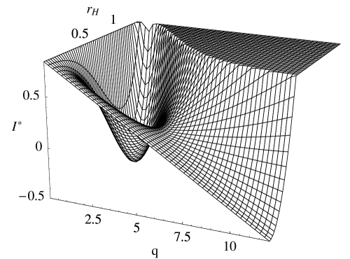
Figure 2: The plot of the action with only one charge turned on. It is plotted against the variables $r_{H}$ and $q$, rather than $e$. The temperature and the (only one) chemical potential are set to $(T,\mu)=(0.45,1.05)$. The local minimum is located at $(r_{H},q)\sim(0.996,1.23)$ and the unstable saddle point is at $(r_{H},q)\sim(0.359,5.38)$. The top flat part simply is a plot range cut-off.

Figure 2 is plotted for the configuration $(e_{1},e_{2},e_{3})=(e,0,0)$ [or $(q_{1},q_{2},q_{3})=(q,0,0)$ through the relations (57)]. The temperature $T:=1/\beta$ and the only chemical potential $\mu$ are set to $(T,\mu)=(0.45,1.05)$. The action falls to minus infinity toward the direction $(r_{H},q)\to(0,\infty)$, therefore, there is no true equilibrium state in this grand canonical ensemble and the local minimum at $(r_{H},q)\sim(0.996,1.23)$ is the metastable black hole. There is an unstable saddle point at $(r_{H},q)\sim(0.359,5.38)$ and it is most likely that the metastable black hole decays by bouncing through this unstable state. In Figure 2, the action appears to go down linearly with respect to $q$. In fact, the action has the $r_{H}\to 0$ limit

$$I^{*}=\beta\Big{\{}\frac{3}{8}+(1-\mu)\,q\Big{\}}+\mathcal{O}(r_{H}^{2})\;.$$ (73)

This expression also shows that the global instability sets in at $\mu=1$. (Notice that Figure 2 is plotted for $\mu=1.05>1$.)

The limit taken in Equation (73) captures the essence of the metastability but it is slightly too simplified, so we now examine the metastable directions in details. For the one charge system in our current consideration, the action $I^{*}$ takes the form

$$I^{*}=\beta\bigg{[}\Big{\{}\,\frac{3}{8}+\frac{3}{2}\,r_{H}^{2}(1+r_{H}^{2}+q)+q\Big{\}}-\sqrt{q(r_{H}^{2}+q)(1+r_{H}^{2})}\;\mu\bigg{]}-2\pi\,r_{H}^{2}\sqrt{r_{H}^{2}+q}\;.$$ (74)

We call the first term in the square bracket, “the mass part”, the second term, “the EM energy”, and the last term in the above expression “the entropy”. As in the standard grand canonical ensemble, the mass part thermodynamically competes against the EM energy and the entropy. We are interested in the direction in the parameter space where the EM energy and the entropy overcome the mass part in the action. It is clear from the form of the action that this can possibly happen only in the direction $q\to\infty$. Expanding the action $I^{*}$ for large $q$, we obtain

$$I^{*}=\beta\Big{(}1+\frac{3}{2}r_{H}^{2}-\sqrt{1+r_{H}^{2}}\;\mu\Big{)}\,q+\mathcal{O}(q^{1/2})\;.$$ (75)

The next-to-leading order is $q^{1/2}$ but we concentrate on the leading term. For fixed values of $\beta$, $\mu$ and $q$, this term has the minimum at $r_{H}=0$ as long as $\mu\leq 3$, and for $\mu\geq 3$, the minimum is located at $r_{H}=\sqrt{\mu^{2}/9-1}$. This means that the most likely direction of the instability is $(r_{H},q)\to(0,\infty)$ for $1<\mu\leq 3$ and is $(r_{H},q)\to(\sqrt{\mu^{2}/9-1},\infty)$ for $\mu\geq 3$. Hence, it appears that the metastable black hole decays either by collapsing to $r_{H}\to 0$ with diverging charge or into some finite horizon radius with diverging charge, depending on the value of $\mu$. However, we suspect that this is not the physical behavior of the decaying black hole. First, the physical meaning of the value $\mu=3/R$ is highly unclear as oppose to $\mu=1/R$ which has the relation to the BPS bound. The second reason is that our analysis is entirely classical and quantum corrections are not considered. Also we have ignored the effect of the back-reaction from the thermal gravitons. We should expect the modifications to the action due to those effects and should not trust the results too much in details without good reasons. Finally, our action can only describe the systems satisfying the assumptions that we have adopted along the derivation of the reduced action. Thus it is possible that a metastable black hole decays into some other spacetime with, say, a different topology or a geometry that is not spherically symmetric. We do know that there is a metastable direction in the parameter space but we cannot simply conclude the decaying process of the unstable black hole using the method adopted in this work.

To summarize, our action shows that the metastability sets in at $\mu=1$ as shown in Equation (73) and a metastable black hole decays by accumulating large amount of charge due to the excessive value of the chemical potential. Though we have neglected the corrections to the action due to the quantum and back reaction effects, we expect that those effects do not modify the qualitative behavior of the system. In particular, as we discussed in the introduction, we have a good reason to expect the critical value of the chemical potential $\mu=1$ receives no corrections. It is commonly assumed that an instability of a system merely implies the existence of a new ground state but our analysis of the theory does not suggest such picture.

4.2 Small Black Hole, Large Black Hole and Instabilities

We now examine the behavior of the stable and unstable saddle points that the boundary reduced action possesses. For the one charge configuration, our action has a saddle point at the values of $r_{H}$ and $q$ that satisfy

$$\beta=\frac{2\pi\sqrt{r_{H}^{2}+q}}{2r_{H}^{2}+1+q}\;,\quad\mu=\sqrt{\frac{q(1+r_{H}^{2})}{r_{H}^{2}+q}}\;.$$ (76)

Since we are considering the grand canonical ensemble, these expressions should be solved for $r_{H}$ and $q$ in terms of given values of $\beta$ and $\mu$, and the solutions are the thermal expectation values of the equilibrium state. There are two relevant solutions with real and positive horizon radii.

In Figure 3, $r_{H}$ of those solutions are plotted in the parameter space of $(T,\mu)$.

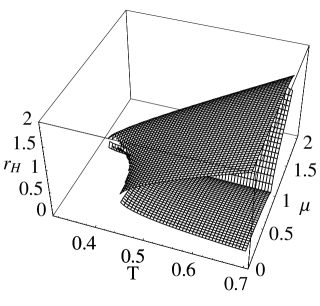
Figure 3: The two relevant solutions, $r_{H}(T,\mu)$, of Equations (76) are plotted and superposed. The top leaf corresponds to the (locally) stable black hole (large black hole) and the other leaf to the unstable black hole (small black hole). The lower leaf has a cusp along the line of $\mu=1$ and the value of the horizon radius along this line is zero. The slight gap between the leaves is due to the numerical noise.

In the blank regions of the parameter space, there are no saddle point solutions to the action. The blank region that surrounds the origin of the diagram corresponds to the part inside of the dotted line in the left diagram of Figure 1. Also the blank region of very large $\mu$ is the local instability part of the phase diagram that corresponds to the region above the solid line of the left diagram in Figure 1. Therefore, if we project Figure 3 down to the $\mu$-$T$ plane, the boundary of the plot is the (local) instability lines discuss in Section 2. The top “leaf” of Figure 3 is the locally stable black hole solution and the other bottom leaf is the unstable saddle point of the action. Those two saddle points of the action are commonly called “large black hole” and “small black hole”, respectively, and we adopt this terminology here. In Figure 4, we also plot the slices of the functions $r_{H}(T,\mu)$ and $q(T,\mu)$ against the chemical potential $\mu$ at the fixed temperature $T=0.45$.

Figure 4: Diagram (a) is plotted for the horizon radii $r_{H}$ of the large and small black holes against $\mu$ at fixed temperature $T=0.45$. The solid line corresponds to the large black hole solution and the dashed line to the small black hole. Similar plot is given in Diagram (b) for the charges $q$ against $\mu$ at the same temperature $T=0.45$ as the other diagram.

Notice, in particular, the behavior of the small black hole at the line $\mu=1$. At this critical metastability line, the small black hole, regardless of the temperature, shrinks to zero size in horizon and ceases to exist. Above the critical line, the small black hole gains finite horizon radius again, but the charge jumps to a bigger value than that of the large black hole. The large and the small black hole saddle points of the action merge at the local instability lines (the solid and dotted lines in the left diagram of Figure 1).

In what follows, we describe the role of the small black hole in different phases. In Section 2, we explained that the region between the dotted and dashed lines in Figure 1 is the spinodal phase where the thermal AdS space without black hole is energetically preferred but the black hole solution remains locally stable. The action $I^{*}$ at the origin of the parameter space $(r_{H},q)$ corresponds to the thermal AdS space without black hole. Therefore, in the spinodal phase, the large black hole saddle point does exist but the value of the action at this point is larger than the value at the origin. There is an unstable small black hole solution between the large black hole and the thermal AdS space in the $(r_{H},q)$ parameter space. Thus, the large black hole in the spinodal phase is most likely to decay into the thermal AdS space, bouncing through the small black hole. The behavior is opposite in the high temperature side of the Hawking-Page phase transition line (the dashed line in Figure 1) and below the metastability critical line $\mu=1$. There, the black hole solution is energetically preferred to the thermal AdS space and the latter is most likely to decay into the large black hole, bouncing through the small black hole. In the region above the $\mu=1$ line and below the local instability line (the solid line in Figure 1), the small black hole is located between the large black hole and the instability direction of the parameter space. Therefore in this region of the phase diagram, the large black hole is most likely to decay into the instability direction bouncing through the small black hole. The thermal AdS space in this phase can either directly decay into instability direction or decay through the large black hole. At the local instability line present above $\mu=1$, the large and small black holes merge and open up the instability direction without any barrier.

To illustrate the described behavior of the saddle points, Figure 5 displays the sequence of the actions with respect to rising chemical potential and fixed temperature $T=0.5$. The numerical data for the diagrams are summarized in Table 2. In the table, “LBH” and “SBH” stand for “Large Black Hole” and “Small Black Hole”, respectively.

Diagram (a) (b) (c) (d) $\mu$ $0.9$ $1$ $1.1$ $1.4$ LBH $(r_{H},q)$ $(1.208,0.7166)$ $(1.211,1.000)$ $(1.205,1.415)$ $(-,-)$ SBH $(r_{H},q)$ $(0.1087,0.1716)$ $(0.000,-)$ $(0.5048,6.885)$ $(-,-)$

Table 2: The numerical data for the plots in Figure 5. The abbreviations “LBH” and “SBH” stand for “Large Black Hole” and “Small Black Hole”, respectively.

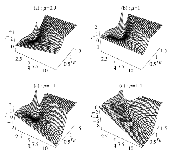
Figure 5: The action is plotted for different values of the chemical potential. For all the diagrams, the temperature is set to $T=0.5$ and other numerical data is shown in Table 2. The top flat parts are the plot range cut-offs.

We comment that the decay processes discussed in this section are similar to the one analysed by Gross et al. [21] where their “Schwarzschild instanton” corresponds to the small black holes in our discussion. The authors of Reference [21] discovered that the Schwarzschild instanton is an unstable saddle point by examining rather general perturbation to the black hole metric. Here we have restricted our consideration to the static and spherically symmetric geometries. Moreover, we have made the very stringent form of metric ansatz and considered very small subspace of the full parameter space. As mentioned near the end of Section 2, reducing the parameter space usually makes it hard to find the unstable directions. Therefore, it is rather remarkable to find the local and global instabilities in our narrow range of analysis.

4.3 Below $T_{0}$

In the regions of the phase diagram discussed above, temperature is always larger than $T_{0}$ at which the horizon radius $r_{H}$ vanishes. The region of the phase diagram below $T_{0}$ has been completely unknown because the analysis was done through the on-shell action which requires the existence of the black hole saddle point. Now that we have the off-shell action, we can discuss this region of the phase diagram. We have two results in this region. One is that the critical line at $\mu=1$ persists at all temperature including below $T_{0}$, and the other is that the black hole saddle points do not exist in this region. These two facts imply that below temperature $T_{0}$, a thermal AdS space decays directly into the instability direction without going through the black hole saddle points, provided that the chemical potential is larger than the inverse of the curvature radius. In fact, one can plot the action for a fixed temperature below $T_{0}$ with chemical potential larger than one and finds a similar plot to Diagram (d) of Figure 5. Therefore, the critical line $\mu=1$ below $T_{0}$ is not the metastability line of a black hole but it is the instability line of the thermal AdS space.

5 Discussions

5.1 AdS/CFT Boundary Temperature

In Section 3.2, we found that the physical boundary temperature red-shifts to zero due to the asymptotic AdS geometry. Therefore, in defining the boundary action, we adopted rather ad hoc rescaled temperature given in Equation (24). We discuss this issue more in detail and argue that the rescaled temperature has a natural interpretation in the sense of AdS/CFT.

The black hole temperature $T_{H}$ computed, for instance, by evaluating the surface gravity at the horizon or by Euclidean continuation to smooth geometry is not a physical temperature in general, and the physical temperature depends on the location of an observer. Therefore, the physical temperature (sometimes called Tolman temperature [29]) is given by

$$T_{\text{physical}}=T_{H}V(r_{B})^{-1/2}\;,$$ (77)

where we have assumed a spherically symmetric black hole geometry with radial coordinate $r$, red-shift factor $V(r)$ and we locate the observer at $r=r_{B}$.

In the case of the asymptotically flat black hole spacetime, the red-shift factor $V(r)$ can be given with the asymptotic behavior $V\to 1$ as $r_{B}\to\infty$. Thus in this case, the Tolman temperature measured at the boundary of the space equals $T_{H}$ and therefore this is commonly considered as the physical temperature on the boundary. The situation is different for the asymptotically AdS black holes. The red-shift factor in this case has the asymptotic behavior $V\to r_{B}^{2}/R^{2}$ with $R$ being the curvature radius of the asymptotic AdS geometry. This AdS red-shift factor causes the gravitational potential that prevents any massive object from escaping to infinity and effectively acts as an infinite box [16]. Also we see in Equation (77) that the same AdS-term red-shift the physical temperature to zero at the boundary and thus $T_{H}$ is not the physical temperature of the boundary observer.

We have mentioned in Section 3.2 that the AdS black hole thermodynamics in the infinite volume has been discussed by adopting the “renormalized” temperature where the temperature is multiplied by the black hole red-shift factor so that the limit $r_{B}\to\infty$ remains finite. However, since $T_{\infty}:=\lim_{r_{B}\to\infty}T_{\text{physical}}V(r_{B})^{1/2}=T_{H}$, the “renormalized” temperature is the temperature $T_{H}$. The original work of Hawking and Page in Reference [16] discusses the thermodynamic properties using $T_{\infty}$ (or $T_{H}$) and also the following works by others have frequently adopted the same convention. (See, for example, Reference [17] and the references cited therein.) As emphasized by many, the redefined temperature $T_{\infty}$ is not the physical temperature of the boundary thermodynamics but as we stated in Section 3.2, there are indications that $T_{\infty}$ somehow is the boundary temperature which is consistent with the thermodynamic properties. The reason why this is so has remained unclear.

Here, we consider this issue in the light of AdS/CFT correspondence. Let us first recall how the conformal redundancy arises on the boundary of AdS space, based on Reference [8]. To make our discussion concrete, let us consider the AdS₅ space with the metric

$$ds_{\text{AdS}}^{2}=\frac{R^{2}}{(1-y)^{2}}\big{[}-(1+y)^{2}dt^{2}+y^{-1}dy^{2}+4yd\Omega_{3}^{2}\big{]}\;,$$ (78)

where the parameter $R$ is a length scale of the geometry and the (dimensionless) time coordinate $t$ is periodically identified. The boundary is given at $y=1$ and the metric is ill-defined for this value of $y$. To obtain the metric that extends over to the boundary, one can multiply the AdS metric with a function $\eta(x)^{2}$ where the function $\eta(x)$ possesses a first order zero at $y=1$. Again, for the sake of concreteness, we choose

$$\eta(x)=\frac{e^{\omega(x)}}{2}(1-y)\;.$$ (79)

Here, $\omega$ is an arbitrary function over the spacetime including the boundary. Then the boundary metric $d\tilde{s}^{2}$ is given by restricting the extended metric to $y=1$, i.e.,

$$d\tilde{s}^{2}=\big{[}\eta(x)^{2}ds_{\text{AdS}}^{2}\big{]}_{y=1}=e^{2\omega}R^{2}(-dt^{2}+d\Omega_{3}^{2})=e^{2\omega}(d\tau^{2}+R^{2}d\Omega_{3}^{2})\;,$$ (80)

where the function $\omega$ now is understood to be defined over the boundary and the last equality is obtained through the analytic continuation to the Euclidean signature by setting $\tau=iRt$. Observe that the boundary metric is unique only up to conformal transformations due to the arbitrary function $\exp(\omega)$. We also see that the boundary topology is $S^{1}\times S^{3}$. If we assume the existence of a conformal field theory on the boundary, the circumference of the $S^{1}$ time circle and the length scale of $S^{3}$ should be respectively interpreted as the inverse temperature and the length scale of the space on which the CFT is supposed to live. However, each of those quantities cannot have physical significance due to the conformal redundancy. A physical quantity of the field theory must be an invariant of the redundancy and in this case, it is given by the ratio of the $S^{1}$ circumference to the length scale of $S^{3}$. In other words, the temperature of the boundary field theory should always be measured in the units of the length scale of the spatial three sphere.

The argument made in the previous paragraph closely parallels our problem of the black hole boundary temperature. The ill-defined nature of the AdS metric at the boundary is directly reflected to the fact that the local inverse temperature $\tilde{\beta}$ defined in Equation (23) diverges at the boundary. Therefore, unlike the asymptotically flat case, the thermodynamics of AdS black holes is not well-defined in the same straightforward manner. In order to define the black hole temperature on the AdS boundary, one could extend the AdS metric as $d\tilde{s}^{2}$ in Equation (80) and this is similar to the definition (24) of the boundary black hole temperature $\beta$. Notice that this could leave the definition of $\beta$ ambiguous by an arbitrary function. However, the boundary metric has conformal symmetry and thus this black hole temperature cannot be a physical one. Therefore we realize that a possible physical black hole temperature at the boundary must be defined as the ratio between the circumference of $S^{1}$ time circle and the length scale of $S^{3}$ at the boundary;

$$\beta_{\text{boundary}}:=\lim_{r_{B}\to\infty}\frac{S^{1}\text{-circumference at }r_{B}}{\text{length scale of }S^{3}\text{ at }r_{B}}=\lim_{r_{B}\to\infty}\frac{\tilde{\beta}}{r_{B}}=\beta\;.$$ (81)

As we alluded in the last equality, the inverse black hole temperature $\beta$ should really be interpreted in this way. [Equivalently, one may regard $\beta$ as the rescaled temperature by an ambiguous function of the sort shown in Equation (79), followed by taking the ratio of it to the length scale of $S^{3}$, which is rescaled in the same way, at the boundary.]

Now the boundary temperature thus defined may not have any relation to the thermodynamics of the black hole in the bulk because it is not the Tolman temperature of the observer at the boundary. What one should be surprised here is that the boundary action $I^{*}$ with the temperature $\beta$ does consistently describe the thermodynamics of the bulk AdS black hole. One could speculate from this that there would be a conformal theory on the boundary with the temperature $\beta$ and this theory has identical thermodynamics as the bulk black hole, i.e., the AdS/CFT correspondence.

The definition of the chemical potential in Equation (29) also is a conformally invariant quantity. To see this, notice that the integral of the gauge field one-form in Equation (25) is a conformal invariant. Then the product $\tilde{\mu}\tilde{\beta}$ is invariant under conformal transformations. Now since we have argued that the boundary temperature $\beta$ is a conformal invariant, so must be the boundary chemical potential $\mu$.

5.2 More General Solution

In Section 3.3, we solved the Hamiltonian constraint equation (52) by adopting the ansatz shown in Equations (54) and (55). Alternatively, we can take the ansatz for the functions $X_{j}(r)$ and $H(r)$ as before but do not assume the form of the function $f(r)$. Then regard the constraint equation (52) as a first order differential equation of $f(r)$ and get the solution

$$f(r)=\, \frac{r^{2}H(r)}{3r^{4}+2\,r^{2}\sum_{j}q_{j}+q_{1}q_{2}+q_{2}q_{3}+q_{3}q_{1}}$$

$$\times\bigg{[}\sum_{j}\frac{e_{j}^{2}}{r^{2}+q_{j}}+r^{2}\Big{\{}3+2\sum_{j}q_{j}+3\,r^{2}\Big{\}}+C\bigg{]}\;,$$ (82)

where $C$ is an integration constant and the length scale is set to $R=1$. The constant $C$ can be determined through the condition in Equation (56) and we have

$$C=-\sum_{j}\frac{e_{j}^{2}}{r_{H}^{2}+q_{j}}-r_{H}^{2}\Big{\{}3+2\sum_{j}q_{j}+3r_{H}^{2}\Big{\}}\;.$$ (83)

Unlike the previous solution to the Hamiltonian constraint equation, the parameters $e_{j}$ and $q_{j}$ are independent parameters of this solution. We can follow the steps taken in Section 3.4 with the new function (5.2) and obtain the boundary reduced action

$$I^{*}= \,\beta\bigg{[}\frac{3}{8}+\frac{1}{2}\sum_{j}q_{j}+\frac{1}{2}(q_{1}q_{2}+q_{2}q_{3}+q_{3}q_{1})+\frac{1}{2}\sum_{j}\frac{e_{j}^{2}}{r_{H}^{2}+q_{j}}$$

$$+\frac{1}{2}\Big{(}3r_{H}^{4}+2r_{H}^{2}\sum_{j}q_{j}+3r_{H}^{2}\Big{)}-\sum_{j=1}e_{j}\mu_{j}\bigg{]}-2\pi r_{H}^{3}\sqrt{H(r_{H})}\;.$$ (84)

In extremizing this action with respect to the parameters $(r_{H},e_{j},q_{j})$, one finds that there are one-parameter family of extrema. In fact, $\partial I^{*}/\partial r_{H}$ is directly proportional to $\sum_{j}\partial I^{*}/\partial q_{j}$ and the equations are not linearly independent. We can solve the six independent equations out of the seven dependent ones and express the solution, for example, as

$$\mu_{j}^{2} =1+\sum_{k\neq j}q_{k}+2r_{H}^{2}-\frac{2\pi r_{H}}{\beta}H_{j}(r_{H})^{-1}\sqrt{H(r_{H})}\;,$$ (85a)

$$e_{j} =\mu_{j}(r_{H}^{2}+q_{j})\;.$$ (85b)

Using a part of equations of motion, we can determine the Lagrange multipliers $b(r)$ and $A_{j\,\tau}(r)$ as

$$b=\frac{\beta}{2\pi}f^{1/2}H^{-1/3}\;,\quad\text{and}\quad A_{j\,\tau}=-i\,\frac{\beta}{2\pi}\Big{(}\frac{e_{j}}{r_{H}^{2}+q_{j}}-\frac{e_{j}}{r^{2}+q_{j}}\Big{)}\;.$$ (86)

We thus have forms of all the fields and it is checked that they, together with the the relations (85), satisfy all the equations of motion including the Maxwell and scalar field equations with a free parameter, say, $\beta$. Furthermore, we have computed the surface gravity at the horizon (with the same analytic continuation as the one mentioned in footnote 17) and consistently obtained

$$\kappa=2\pi/\beta\;.$$ (87)

Also the thermodynamic identity can be shown to be satisfied, just as we have done at the end of Section 3.4. Parenthetically, the solution satisfies the smoothness condition (21) as we imposed in obtaining the reduced action.

The asymptotic behavior of the function $f(r)$ is

$$f(r)=r^{2}+\Big{(}1+\sum_{j}q_{j}\Big{)}+\mathcal{O}\Big{(}\frac{1}{r^{2}}\Big{)}\;.$$ (88)

Up to this order, this agrees with the asymptotic behavior of the solution obtained in Section 3.3 and in particular, the first term is consistent with the asymptotic condition (22). One can check that the function $f(r)$ takes the form in Equation (54) if and only if the relations (57) hold. So while new $f(r)$ is parametrized by the independent parameters $(r_{H},e_{j},q_{j})$, the previous one is recovered by restricting the new function to the subset of the parameters by the relation (57). As we have seen in Section 3.4, this relation reproduces the solution discussed in Section 2. Therefore, we have obtained the more general solution that include the previous solution as a special case.

What is perhaps odd about this solution is that the grand canonical thermodynamic data, $(\beta,\mu_{j})$, cannot uniquely specify the properties of the black hole. Stated differently, the black hole can be uniquely characterized by the parameters, $(E,e_{j},q_{1})$, where $E$ is the thermodynamic mean energy derived from the action and we have chosen $q_{1}$ to be the free parameter of the degenerate solution (85). Thus, the degeneracy seems to indicate a scalar hair of the black hole. But this conclusion sharply contradicts with the no-hair theorem of Sudarsky and Gonzalez [31]. They have shown that there cannot be scalar hairs for an asymptotically AdS black hole where the scalar potential approaches the global minimum near the boundary. Our scalar potential $V$ in (17) with the solutions $X_{j}$ in (54) actually has such asymptotic behavior. How can this be? One possibility is that the degenerate solution presented in this subsection is equivalent to the known solution through some reparametrization (we have not been able to find such reparametrization). Another possibility is that the no-hair theorem is somehow evaded in our theory, for example, due to the coupling of the scalar to the Abelian gauge fields (such coupling was not considered in Reference[31]). Clarifying this issue requires further considerations separate from the topic of this work.

5.3 On Finite Counterterm

In Section 3.4, we added the term called “finite counterterm” as shown in Equation (64). The original motivation for including the finite counterterm is as follows. Buchel and Pando Zayas [13] observed that when the mass of the $R$-charged AdS black hole was computed using the standard counterterms, an unexpected nonlinear term with respect to the charge appeared. (The charge referred here is the parameter $q$ and not $e$.) This nonlinear behavior of the charge in the mass can contradict the BPS-expected inequality between the mass and the charge, and more importantly, the thermodynamic identity is violated. By requiring the identity to hold, they added a term that consequently eliminated the nonlinear term. Then Liu and Sabra pointed out in Reference [15] that the inclusion of the counterterm associated with the presence of the scalar fields is possible. They showed that the mass computed with the finite counterterm (64) reproduced the result obtained by Buchel and Pando Zayas.

The counterterms that arise from the presence of matter fields are further studied by Batrachenko et al. in Reference [32] utilizing the Hamilton-Jacobi method. In this approach, the counterterms are treated uniformly throughout different spacetime dimensions and in particular, they have found that the scalar field counterterms are divergent, finite and vanishing for the spacetime dimensions four, five and higher, respectively. Note that the inclusion of the scalar counterterm in four dimension is necessary to render the action finite. Thus, it appears natural to include the scalar counterterm for the case of five dimensions but it still requires physical interpretation.

Liu and Sabra in Reference [15] mentioned that the option to include (or not to include) the finite counterterm in five dimension can be interpreted as the counter part to the choice of a renormalization scheme in a field theory. Since the inclusion of the finite counterterm results in the mass that has the BPS-like mass-charge relation, they argued that the counterterm corresponds to the renormalization scheme that preserves the supersymmetry of the boundary field theory. If this interpretation is valid, the physical observables should not be affected by the finite counterterms just as the choice of the renormalization scheme does not affect the physical observables of a field theory.

In our work, we have derived the action that describes the thermodynamics of the black hole observed at the boundary. The AdS/CFT conjecture postulates that the exponential of (minus) the action is the partition function of the dual field theory at strong coupling. Then the thermal mean values derived from the action, such as $\langle E\rangle$ or $\langle Q_{j}\rangle$ of Equation (70) must be the physical observables of the thermal field theory. However, we see that the addition of the finite counterterm does affect the thermal mean values. It is most clearly seen in the charges

$$\langle Q_{j}\rangle=e_{j}=\sqrt{q_{j}(r_{H}^{2}+q_{j})\bigg{\{}1+r_{H}^{2}\prod_{k\neq j}H_{k}(r_{H})\bigg{\}}}\;.$$ (89)

This expression is derived from the metric ansatz and the Hamiltonian constraint equation, so the form is independent of the counterterms. But the numerical value does change by the presence and absence of the finite counterterm because the location of the extremum is affected. Similar argument applies to the other mean values. Therefore, the observables of the theory do seem to depend on the finite counterterm.

The dependence may imply that the finite counterterm has different physical interpretation. Another possibility is that the contributions to the partition function from other saddle points may make the physical observable independent of the finite counterterm. In any case, the observation made here urges us to investigate the physical interpretation of the finite counterterm and better understanding is desired.

5.4 Comparison to the Field Theory Analysis

In this work, we have found an additional structure in the phase diagram of $R$-charged black hole system. The phase diagram in Figure 1 is now augmented by the line $\mu=1/R$ that separates the stable and metastable black hole states for $T>T_{0}$ and below $T_{0}$, the same line is the instability critical line of the thermal AdS space. As mentioned in the introduction, the existence of the metastable black hole has been anticipated from the AdS/CFT-conjectured field theory analysis in Reference [9]. The current status of the phase diagrams in the gravity and field theory sides is schematically summarized in Figure 6.

Figure 6: The schematic phase diagram of the $R$-charged black hole is shown on the left-hand side and on the right-hand side, that of the field theory which is supposed to be the AdS/CFT dual is shown. According to the AdS/CFT correspondence, the black hole system is identical to the strongly coupled region of the field theory, as indicated in the diagram. For both figures, $\mu$ is the largest of the three chemical potentials. In the strong coupling diagram, $T_{0}$ is the temperature at which the black hole radius reaches to zero. Its value depends on the pattern of chemical potentials and equals $(\pi R)^{-1}$ for a single non-zero charge, while $T_{0}=0$ for three equal charges. On the other hand, the nature of the instability in the low temperature regime of the weakly coupled field theory is yet to be explored and is indicated by the dashed line in the diagram.

We see the agreement in the general structure of those phase diagrams and the additional match in the metastability critical line $\mu=1/R$ is the improvement made in this work.

In Section 4.3 we saw that in the region of the phase diagram below $T_{0}$, a thermal AdS space decays directly into unstable direction without going through the black hole saddle points. The corresponding field theory analysis has not been carried out at the low temperature. However, given the result of the gravity analysis, we have some expectations for the behavior of the field theory. First we note that the “confinement/deconfinement” phase transition line is obtained in the zero coupling limit of the field theory. The phase transition line and the $\mu=1$ line merge exactly at $T=0$. The zero coupling limit is taken so that the resulting free theory is continuously connected to the theory with finite coupling constant. Thus we expect the general structure of the phase transition line to remain the same at a finite coupling, but it is likely that the details would change. For instance, it is possible that the phase transition line at the finite coupling is modified so that it merges with the instability line at some finite temperature. This behavior could be similar to the one observed in the gravity analysis. To verify this expectation, one needs to find the confinement/deconfinement phase transition line at weak but finite coupling with nonzero chemical potentials and also the instability line at the low temperature region must be determined. We believe that the analysis, especially in the low temperature limit, is doable and the work is in progress.

In the field theory analysis of Reference [9], it has been found that the decay of a metastable state is most likely to occur by one of the eigenvalues of the scalar field splitting up from the rest of the eigenvalues in the field space and indefinitely growing. Our analysis in this paper does not necessarily suggest this mechanism. If we attempt to interpret this phenomenon in terms of string theory, it would correspond to a D3-brane separating from a stack of rotating D3-branes due to the high angular velocity of the D3-branes in their transverse directions. Therefore, we could also detect the metastability by examining the behavior of a probe D3-brane immersed in the background of the $R$-charged black hole or of the rotating D3-branes (before taking the decouping limit). This scenario is currently being investigated.

Both gravitational and field theory analysis show that two theories cease to exist above the critical value of the chemical potential where the local instability sets in. In the AdS/CFT context, this means that the theory at strong and weak coupling regimes both become unstable at a large value of the chemical potential. One might naively interpolate the results and speculate that the theory in any coupling regime is unstable beyond a certain value of the chemical potential. Though we think that this is the most likely scenario, we still cannot completely exclude the possibility that the theory develops a new ground state beyond the instability line and defines a Higgs phase. As mentioned in Section 4, we did not take into account of the back reaction from the thermal radiation and also the quantum corrections are neglected. (Needless to say, stringy effects have not been considered which we expect to be important when $r_{H}$ becomes comparable to the length scale of string theory.) On the field theory side, the analysis has been carried out at one-loop level and higher loop with finite $N_{c}$ effects are still unknown. They may or may not change the global behavior of the potential in the theory.

Appendix A Metastability in General Charge Configuration

In the main text, the metastability of the $R$-charged black hole is examined in the subspace of the full parameter space with the only one nonzero charge. This appendix augments the argument that the metastable black hole system with a general charge configuration tends to have the unstable direction into the single charge configuration.

As in the single charge case of the main text, a possible instability occurs only when one of the charges diverges. This is because the $r_{0}$ factor in $E$ of Equation (69) overwhelms the rest of the terms when more than one charges become large. Therefore, without loss of generality, we expand the action with respect to large $q_{1}$ to obtain

$$I^{*}=\beta\Big{(}1+\frac{3}{2}x_{1}^{2}-\sqrt{1+x_{1}^{2}}\;\mu_{1}\Big{)}\,q_{1}+\mathcal{O}(q_{1}^{1/2})\;,$$ (90)

where we have defined the parameter $x_{1}:=r_{H}^{2}H_{2}(r_{H})H_{3}(r_{H})$. This is exactly the same form as in Equation (75) and therefore, for fixed values of $\beta$, $\mu_{1}$ and $q_{1}$, the leading term has the minimum at $x_{1}=0$ as long as $\mu_{1}\leq 3$, and for $\mu_{1}\geq 3$, the minimum is located at $x_{1}=\sqrt{\mu_{1}^{2}/9-1}$. This implies that as long as $1<\mu_{1}\leq 3$, the unstable direction is $(r_{H},q_{1},q_{2},q_{3})\to(0,\infty,0,0)$ and for $\mu_{1}\geq 3$, the parameters $r_{H}$, $q_{2}$ and $q_{3}$ may be nonzero but none of them may diverge. One of the consequences of this consideration is that the constrained system with $q_{1}\equiv q_{2}\,,\;q_{3}\equiv 0$ or $q_{1}\equiv q_{2}\equiv q_{3}$ does not have the global instability (and as mentioned near the end of Section 2, these configurations do not have the local instabilities as well). Those constraints reduce the dimension of the parameter space and the unstable directions are closed. The discussion made in this paragraph is illustrated in Figure 7 for the case with the two nonzero charges.

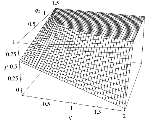
Figure 7: In this plot of the action, the configuration with $q_{3}\equiv 0$ is chosen. The temperature, the horizon radius and the chemical potentials are set to $T=0.6$, $r_{H}=0.01$ and $(\mu_{1},\mu_{2})=(1.2,0.85)$, respectively. The diagram shows that an instability exists only in the direction of the large charge whose corresponding chemical potential exceeds the critical value $1$. It also exhibits that the direction along $q_{1}=q_{2}$ is stable. The top flat part is a plot range cut-off.

Observe that the instability direction opens up for the large charge whose conjugate chemical potential is larger than one. In this plot, it is the direction of large $q_{1}$ and not $q_{2}$. Also note that the action does not have instability along the line $q_{1}=q_{2}$.

The result obtained in this appendix confirms the claim made in the main text; the metastability in the case with general charge configurations essentially boils down to the system with one charge.

References

- [1] H. W. Braden, J. D. Brown, B. F. Whiting and J. W. York, Charged Black Hole In A Grand Canonical Ensemble, Phys. Rev. D 42, 3376 (1990).
- [2] M. Pernici, K. Pilch and P. van Nieuwenhuizen, Gauged D = 5 Supergravity, Nucl. Phys. B 259, 460 (1985).
- [3] M. Gunaydin, L. J. Romans and N. P. Warner, Gauged Supergravity In Five-Dimensions, Phys. Lett. B 154, 268 (1985).
- [4] A. Chamblin, R. Emparan, C. V. Johnson and R. C. Myers, Charged AdS black holes and catastrophic holography, Phys. Rev. D 60, 064018 (1999) [arXiv:hep-th/9902170].
- [5] M. Cvetic and S. S. Gubser, Phases of R-charged black holes, spinning branes and strongly coupled gauge theories, JHEP 9904, 024 (1999) [arXiv:hep-th/9902195].
- [6] J. M. Maldacena, The large N limit of superconformal field theories and supergravity, Adv. Theor. Math. Phys. 2, 231 (1998) [Int. J. Theor. Phys. 38, 1113 (1999)] [arXiv:hep-th/9711200].
- [7] S. S. Gubser, I. R. Klebanov and A. M. Polyakov, Gauge theory correlators from non-critical string theory, Phys. Lett. B 428, 105 (1998) [arXiv:hep-th/9802109].
- [8] E. Witten, Anti-de Sitter space and holography, Adv. Theor. Math. Phys. 2, 253 (1998) [arXiv:hep-th/9802150].
- [9] D. Yamada and L. G. Yaffe, Phase diagram of super-Yang-Mills theory with R-symmetry chemical potentials, JHEP 0609, 027 (2006) [arXiv:hep-th/0602074].
- [10] D. Yamada, Quantum mechanics of lowest Landau level derived from SYM with chemical potential, arXiv:hep-th/0509215.
- [11] T. Harmark and M. Orselli, Quantum mechanical sectors in thermal super Yang-Mills on , Nucl. Phys. B 757, 117 (2006) [arXiv:hep-th/0605234].
- [12] K. Behrndt, M. Cvetic and W. A. Sabra, Non-extreme black holes of five dimensional AdS supergravity, Nucl. Phys. B 553, 317 (1999) [arXiv:hep-th/9810227].
- [13] A. Buchel and L. A. Pando Zayas, Hagedorn vs. Hawking-Page transition in string theory, Phys. Rev. D 68, 066012 (2003) [arXiv:hep-th/0305179].
- [14] J. D. Brown and J. W. York, Quasilocal energy and conserved charges derived from the gravitational action, Phys. Rev. D 47, 1407 (1993).
- [15] J. T. Liu and W. A. Sabra, Mass in anti-de Sitter spaces, Phys. Rev. D 72, 064021 (2005) [arXiv:hep-th/0405171].
- [16] S. W. Hawking and D. N. Page, Thermodynamics Of Black Holes In Anti-De Sitter Space, Commun. Math. Phys. 87, 577 (1983).
- [17] D. R. Brill, J. Louko and P. Peldan, Thermodynamics of -dimensional black holes with toroidal or higher genus horizons, Phys. Rev. D 56, 3600 (1997) [arXiv:gr-qc/9705012].
- [18] J. D. Brown, J. Creighton and R. B. Mann, Temperature, energy and heat capacity of asymptotically anti-de Sitter black holes, Phys. Rev. D 50, 6394 (1994) [arXiv:gr-qc/9405007].
- [19] R. Wald, General Relativity, The University of Chicago Press, 1984
- [20] D. J. Gross, R. D. Pisarski and L. G. Yaffe, QCD And Instantons At Finite Temperature, Rev. Mod. Phys. 53, 43 (1981).
- [21] D. J. Gross, M. J. Perry and L. G. Yaffe, Instability Of Flat Space At Finite Temperature, Phys. Rev. D 25 (1982) 330.
- [22] R. Arnowitt, S. Deser and C. Misner, The Dynamics of General Relativity in Gravitation: An Introduction to Current Research, Ed. L. Witten, New York: Wiley, 1962
- [23] G. W. Gibbons and S. W. Hawking, Action Integrals And Partition Functions In Quantum Gravity, Phys. Rev. D 15, 2752 (1977).
- [24] M. Henningson and K. Skenderis, The holographic Weyl anomaly, JHEP 9807, 023 (1998) [arXiv:hep-th/9806087].
- [25] V. Balasubramanian and P. Kraus, A stress tensor for anti-de Sitter gravity, Commun. Math. Phys. 208, 413 (1999) [arXiv:hep-th/9902121].
- [26] R. Emparan, C. V. Johnson and R. C. Myers, Surface terms as counterterms in the AdS/CFT correspondence, Phys. Rev. D 60, 104001 (1999) [arXiv:hep-th/9903238].
- [27] M. Cvetic et al., Embedding AdS black holes in ten and eleven dimensions, Nucl. Phys. B 558, 96 (1999) [arXiv:hep-th/9903214].
- [28] C. S. Peca and J. P. S. Lemos, Thermodynamics of Reissner-Nordstroem-anti-de Sitter black holes in the grand canonical ensemble, Phys. Rev. D 59, 124007 (1999) [arXiv:gr-qc/9805004].
- [29] R. Tolman, On the Weight of Heat and Thermal Equilibrium in Genral Relativity, Phys. Rev. 35, 904 (1930)
- [30] E. Witten, Anti-de Sitter space, thermal phase transition, and confinement in gauge theories, Adv. Theor. Math. Phys. 2, 505 (1998) [arXiv:hep-th/9803131].
- [31] D. Sudarsky and J. A. Gonzalez, On black hole scalar hair in asymptotically anti-de Sitter spacetimes, Phys. Rev. D 67, 024038 (2003) [arXiv:gr-qc/0207069].
- [32] A. Batrachenko, J. T. Liu, R. McNees, W. A. Sabra and W. Y. Wen, Black hole mass and Hamilton-Jacobi counterterms, JHEP 0505, 034 (2005) [arXiv:hep-th/0408205].