Cycling in the Throat

Abstract:

We analyse the dynamics of a probe D3-(anti-)brane propagating in a warped string compactification, making use of the Dirac-Born-Infeld action approximation. We also examine the time dependent expansion of such moving branes from the “mirage cosmology” perspective, where cosmology is induced by the brane motion in the background spacetime. A range of physically interesting backgrounds are considered: AdS₅, Klebanov-Tseytlin and Klebanov-Strassler. Our focus is on exploring what new phenomenology is obtained from giving the brane angular momentum in the extra dimensions. We find that in general, angular momentum creates a centrifugal barrier, causing bouncing cosmologies. More unexpected, and more interesting, is the existence of bound orbits, corresponding to cyclic universes.

1 Introduction

One of the biggest challenges remaining for early universe cosmology is to find a compelling explanation for inflation, or rather, an explanation for the initial perturbation spectrum of our universe, as inferred from the microwave background. Until recently, models for inflation were somewhat empirically motivated, using various phenomenological scalar fields, with parameters almost as fine tuned as those initial conditions inflation was designed to circumvent [1]. In the past few years, string theory has entered the fray of finding a convincing arena for inflationary cosmology. In the past, applying string theory to the early universe was beset by many problems, not least that of stabilising moduli [2]. String theory is set most naturally in more than four dimensions, and the challenge is to explain why we do not see those extra dimensions. Nonetheless, applying stringy ideas to the early universe has led to many interesting ideas, such as a possible explanation of the dimensionality of spacetime, [3], resolutions of the initial singularity via duality [4], and the idea that we do not see the extra dimensions because we are confined to live on a braneworld [5, 6].

Whether or not we live on a brane, stabilising extra dimensions is very much an issue, and early on it was realised in supergravity that fluxes living in the extra dimensions could stabilise the compactification [7]. In fact, this idea has been used to attempt to tune the cosmological constant in braneworld models [8]. Meanwhile, in string theory, the AdS/CFT correspondence [9] has driven an exploration of new supergravity backgrounds, dual to various gauge theories, several of which have the supergravity D-brane sources replaced by fluxes on the background manifold [10, 11]. The effect of these fluxes is to replace the AdS horizon typically present in the supergravity D-brane solution by a smooth throat, which, in the Klebanov-Strassler [11] case, smoothly closes off the geometry. Given the relation, [12], between the AdS/CFT correspondence and the Randall-Sundrum [13] braneworld model, it is natural that a neat description of hierarchies in flux compactifications in string theory should use the concept of warping [14].

Most recently, many of these ideas have dovetailed together in what is dubbed the KKLT scenario [15]. Although this description is inherently stringy, it also corresponds to concrete supergravity realisations, and can therefore be used as a setting for exploring possible braneworld cosmologies. For example, the early brane inflation models [16] can be set in this context to get stringy brane inflation, as in [17]. In these scenarios, the brane location on the internal manifold is promoted to a scalar field in our effective cosmology, hence motion on the internal manifold is key to determining the dynamics of inflation. Indeed, the warping induced by the stabilising fluxes plays a crucial role in providing a sufficient period of inflation: it reduces the size of parameters related to the inflationary potential, rendering it flat enough to satisfy the slow roll conditions.

A D-brane or anti-brane wandering on a warped throat experiences another interesting effect, namely the existence of a “speed limit” [18] on the motion of the brane which results from a constraint imposed by the non-standard form of the DBI brane action. This means that the contribution of the kinetic terms can become negligible compared to the potential terms in the brane action, which then dominate and can drive inflation. Besides the potential cosmological applications of this effect, it is interesting to explore the effects of a non-standard DBI brane action for the trajectories of branes in warped backgrounds in more generality.

One key lesson learned from empirical braneworld models, such as Randall-Sundrum, is that brane cosmology is achieved by having branes moving in a curved background spacetime [19], indeed, in the case of the RS model, the cosmological problem can be completely and consistently solved for the brane and bulk, as the system is integrable, [20], giving rise to a “non-conventional” Friedman equation on the brane [21]. Unfortunately, this beautiful simplicity is destroyed by the addition of extra fields, [22], or extra co-dimensions [23], such as would be present in a stringy compactification. Nonetheless, the mirage approach to brane cosmology, [24] is a fascinating proposal in which we ignore the full gravitational consistency of a particular moving brane solution (somewhat justified in the case of a single brane for which the supergravity solution is somewhat suspect in any case unless at distances larger than the compactification scale) and simply lift the concept of cosmology as motion to higher codimension. In this picture, our Universe is a probe brane moving in some supergravity background, and the induced metric in the four non-compact dimensions is therefore time dependent by virtue of this motion. This time dependent metric therefore has the interpretation of a cosmology, and the effective energy momentum (given by computing the Ricci curvature of this induced metric) is the mirage matter source on the brane. This picture – defined and developed in [24] – has been the basis for much work on probe-brane cosmology in string theory.

The key feature of probe brane (or indeed interacting brane) calculations is that the location of the brane on the compact manifold acts as a four-dimensional scalar field in our non-compact four-dimensional Universe. This scalar field has a well prescribed action (in the probe brane case) given by the Dirac-Born-Infeld action for the kinetic terms, and a Wess-Zumino term [25]. These together give an attractive potential in the case of an anti-D3-brane, such as the KKLMMT model [17], or a velocity dependent potential in the case of a D3-brane [18]. In many ways, this latter case is reminiscent of the ideas of kinetic inflation [26]. The idea is to use the motion of the wandering brane on the internal manifold to generate cosmological evolution, or (equivalently) to use the additional energy momentum of the brane as a cosmological source, and analyse the importance of stringy features, such as the DBI action, or particular warped backgrounds, such as the Klebanov-Tseytlin (KT) [10] or Klebanov-Strassler (KS) [11] throats.

The KT and KS solutions are based on the conifold background of string theory [27]. The Klebanov-Tseytlin solution describes a singular geometry produced by $N$ D3-branes and $M$ D5-branes wrapping a (vanishing) 2-cycle of the conifold (fractional D3-branes). The Klebanov-Strassler solution is a smooth supergravity solution in which the conifold base of KT has been replaced by the deformed conifold (see [27]), giving a differential warping in the internal ‘angular’ directions of the space. Both metrics asymptote anti-de Sitter space in the UV, are equivalent at intermediate scales, but in the IR the KT solution has a singularity at its tip, whereas KS rounds off smoothly (see figure 9).

Probe brane analysis with an eye on possible cosmological applications, initiated by the mirage work [24, 28], was started in the context of warped compactifications in [29], where a D3-brane moving radially on the KS background was analysed. The key discovery was that the brane ‘bounced’ (i.e. simply fell to the bottom of the throat and came back out again) and hence the cosmology passed from a contracting to an expanding phase. This gives an alternative realisation to earlier superstring cosmology ideas [4], which also featured an initial singularity avoiding bounce. Note, this bounce is quite distinct from the “Big Crunch – Big Bang” type of bounce typical of colliding brane scenarios [30], in which there is an issue, yet to be satisfactorily resolved, of continuation through the singular collision [31], which is vital to obtaining the correct cosmological perturbation spectrum.

Further work on cosmological branes has attempted to take backreaction into account [32] (although the validity of any supergravity approach at small scales is problematic). For example, in [18] (see also [36]), standard gravitational couplings of the brane scalar field were considered, and candidate potential terms for the scalar field. In most cases, a radial motion of the brane is considered, i.e. the brane simply moves ‘up’ or ‘down’ the warped throat. However, since the internal manifold has five other internal dimensions, it is natural to consider the effect of angular motion on the brane (as originally anticipated in [24]). Typically, angular momentum gives rise to centrifugal forces, hence we might expect brane bouncing to be ubiquitous for orbiting branes. Indeed, in [33] it was argued that this was the case by considering a (Schwarzschild) AdS${}_{5}\times S^{5}$ background. Also, in the case of Branonium [34], a bound state of an orbiting anti-D3-brane, angular momentum was crucial in obtaining this (unstable) bound state. (See also [35].)

The aim of the present work is to extend previous analyses and study the effects of angular momentum on the probe brane motion specifically in warped Calabi-Yau throats. Recall that the location of the brane on the internal manifold will become the inflaton in a fully realistic description of brane cosmology. However, because the angular directions in the internal manifold correspond to Killing vectors of the geometry, the angular variables per se are not dynamical variables from the 4D cosmological point of view. Thus, the inflaton in our models is precisely the same as the inflaton in the KKLT-based models, what is new is that angular momentum provides additional potential terms for the inflaton. So far, angular motion has only explicitly been considered for the case of an AdS${}_{5}\times S^{5}$ background [37], or the AdS-Schwarzschild${}_{5}\times S^{5}$ [33], although in [37] the slow motion (i.e. non DBI) approximation in a KS throat was considered. The KS throat already exhibits a bouncing universe, but we expect angular momentum to induce a bounce at a larger value of the scale factor. We are also interested in whether there are any qualitatively new features for orbiting branes, for example, the branonium is a rather different qualitative solution for an anti-D3 brane to the inflationary solution of KKLMMT.

We find a resounding affirmative outcome to these two investigations. As with Germani et al. [37], we find that the effect of orbital motion in the DBI action is to slow down the brane radial velocity. This slowing is crucial for having bounces as used in their slingshot scenario. However, more interestingly we find qualitatively new behaviour for orbiting branes, which can now have bound states in the IR region of the KS and KT throats. We stress that these are branes and not anti-branes, hence quite distinct from the branonium set-up. These solutions have the cosmological interpretation of cyclic universes (though without the big bang collision of the more controversial cyclic scenario [38]).

The organisation of the paper is as follows. In the next section we present the general set up we are considering. We derive the Hamiltonian for the brane (or antibrane) moving on a generic background. We also discuss the qualitative brane motion, and the effect of angular momentum. We then turn to three main examples of brane motion. In section three, we analyse brane motion in anti-de Sitter space as a warm up exercise. In sections four and five, we then turn to explicit SUGRA backgrounds which modify the IR behaviour of the AdS spacetime: the (singular) Klebanov-Tseytlin (KT), and the (regular) Klebanov-Strassler (KS) metrics. The main result we find is that angular momentum introduces additional turning points in the radial motion of the brane – allowing for bouncing, or no big bang cosmologies. This result is no surprise, after all, angular momentum generically introduces centrifugal barriers. However, what is surprising is that we find regions of parameter space where bound orbits can occur – i.e. cyclic cosmologies. We show that there are bound states of the D3 probe brane in the KS background which correspond to cyclic cosmologies. In the final section we summarize and comment on the effect of back-reaction.

2 Probe brane analysis: General set up

In this section we derive the general action and equations of motion for a probe D3 or anti-D3-brane moving through a type IIB supergravity background describing a configuration of branes and fluxes. A probe brane analysis is self consistent when we consider a single brane moving in a background made by a large numbers of other branes. Our approximations are valid provided we remain both within the string perturbation theory regime, i.e. the string coupling $g_{s}(r)=g_{s}\,e^{\phi(r)}$ is everywhere small, and within the supergravity limit, i.e. in regimes of small curvatures. In our case, this is true provided the number of branes and/or fluxes in the background is large enough, so that the curvatures are kept small. We will make this statement precise in the particular examples we consider in the next sections.

We start by specifying the Ansatz for the background fields we consider, and the form of the brane action. We are interested in compactifications of type IIB theory, in which the metric takes the following general form (in the Einstein frame)

$$ds^{2}=h^{-1/2}\,\eta_{\mu\nu}\,dx^{\mu}dx^{\nu}+h^{1/2}\,g_{mn}dy^{m}dy^{n}\,.$$ (1)

Here $h$ is the warp factor, which in the examples we are considering, depends only on a single, radial, combination of the internal coordinates $y^{m}$, dubbed $\eta$. The internal metric $g_{mn}$ depends on the internal coordinates $y^{m}$, however, this dependence is consistent with a compact ‘angular’ symmetry group of the underlying spacetime, so that particle or brane motion has conserved angular momenta. The field strengths that can be associated with a metric of this form are $F_{1}$, $F_{3}$, $H_{3}$ and $F_{5}$. These fields have only internal components, apart from $F_{5}$, which can assume the form

$$F_{5}=dC_{4}=g_{s}^{-1}dh^{-1}\wedge dx^{0}\wedge dx^{1}\wedge dx^{2}\wedge dx^{3}\ +\quad{\rm dual}.$$

Besides these fields, the dilaton can also be active and in general is a function of the radial coordinate only, $\phi=\phi(\eta)$.

We now embed a probe D3-brane (or an anti-brane) in this background, with its four infinite dimensions parallel to the four large dimensions of the background solution. The motion of such a brane is described by the sum of the Dirac-Born-Infeld (DBI) action and the Wess-Zumino (WZ) action. The DBI action is given, in the string frame, by

$$S_{DBI}=-T_{3}\,g_{s}^{-1}\int{d^{4}\xi\,e^{-\phi}\sqrt{-det(\gamma_{ab}+{\mathcal{F}}_{ab})}}\,,$$ (2)

where ${\mathcal{F}}_{ab}={\mathcal{B}}_{ab}+2\pi\alpha^{\prime}\,F_{ab}$, with ${\mathcal{B}_{2}}$ the pullback of the 2-form field to the brane and $F_{2}$ the world volume gauge field. $\gamma_{ab}=g_{MN}\,\partial_{a}x^{M}\partial_{b}x^{N}$, is the pullback of the ten-dimensional metric $g_{MN}$ in the string frame. Finally $\alpha^{\prime}=\ell_{s}^{2}$ is the string scale and $\xi^{a}$ are the brane world-volume coordinates.

This action is reliable for arbitrary values of the gradients $\partial_{a}x^{M}$, as long as these are themselves slowly varying in space-time, that is, for small accelerations compared to the string scale (alternatively, for small extrinsic curvatures of the brane worldvolume). In addition, recall that the string coupling at the location of the brane should be small, i.e. $g_{s}\ll 1$.

The WZ part is given by

$$S_{WZ}=q\,T_{3}\,\int_{\mathcal{W}}{C_{4}}\,,$$ (3)

where ${\mathcal{W}}$ is the world volume of the brane and $q=1$ for a probe D3-brane and $q=-1$ for a probe anti-brane.

We are interested in exploring the effect of angular momentum on the motion of the brane, and therefore assume that there are no gauge fields living in the world volume of the probe brane, $F_{ab}=0$. For convenience we take the static gauge, that is, we use the non-compact coordinates as our brane coordinates: $\xi^{a}=x^{\mu=a}$. Since, in addition, we are interested in cosmological solutions for branes, we consider the case where the perpendicular positions of the brane, $y^{m}$, depend only on time. Thus

$$\gamma_{00}=g_{00}+g_{mn}\dot{y}^{m}\dot{y}^{n}\,h^{1/2}=-h^{-1/2}\left(1-hv^{2}\right)$$ (4)

and ${\mathcal{B}}_{ab}=0$. Hence

$$S_{DBI}=-T_{3}\,g_{s}^{-1}\int{d^{4}x\,e^{-3\phi}\sqrt{1-h\,v^{2}}}\,.$$ (5)

in the Einstein frame.

Finally, summing the DBI and WZ actions, we have the total action for the probe brane

$$S=-T_{3}g_{s}^{-1}\int{d^{4}x\,h^{-1}\left[e^{-3\phi}\,\sqrt{1-h\,v^{2}}-q\right]}\,.$$ (6)

This action is valid for arbitrarily high velocities. Note, the expression for the brane acceleration, as defined in [18], is

$$a\sqrt{\alpha^{\prime}}\,=\,h^{\frac{1}{4}}\frac{d}{dt}\left(h^{\frac{1}{2}}v\right)$$ (7)

we recall that this has to be small compared to the string scale for the configurations we are going to analyse. This can be simplified using (17), to:

$$a\sqrt{\alpha^{\prime}} = h^{\frac{1}{4}}\frac{d}{dt}\left(\frac{h\varepsilon\left(h\varepsilon+2q\right)}{\left(h\varepsilon+q\right)^{2}}\right)^{\frac{1}{2}}\,$$ (8)

$$= \frac{2h^{\prime}h^{\frac{1}{4}}\varepsilon}{(\varepsilon h+q)^{2}}\,\dot{\eta}\,$$

$$= \frac{2\,h^{\prime}h^{\frac{1}{4}}\varepsilon(g^{\eta\eta})^{1/2}}{\left(\varepsilon h+q\right)^{3}}\left[\varepsilon\left(h\varepsilon+2q\right)-\ell^{2}(\eta)\right]^{1/2}\,.$$

2.1 Brane Dynamics and the Effect of the Angular Momentum

The above action can be interpreted as describing the dynamics of a particle of mass $m$ moving in the internal transverse space dimensions, with Lagrangian

$${\mathcal{L}}=-m\,h^{-1}\left[\sqrt{1-h\,v^{2}}-q\right]\,.$$ (9)

Here, $m=T_{3}\,V_{3}g_{s}^{-1}$, and $V_{3}=\int{d^{3}x}$ is the volume of the D3 brane. The non canonical form of the kinetic terms has interesting effects for the dynamics of the brane, especially in the regime where the warp factor $h$ is large. Indeed, the quantity $1-hv^{2}\geq 0$ must remain positive in order to have a real Lagrangian, and this imposes a bound on the brane “speed” $v$. Note that while the brane speed depends on both the radial and the angular coordinates of the manifold, it is only the radial coordinate $\eta$, and its velocity that is of cosmological importance, since that is what becomes the inflaton. Therefore, in what follows, we focus on the properties of the radial velocity.

The aim of the present work is to investigate some consequences of the DBI-form of the Lagrangian when we allow the brane to move along the internal ‘angular’ directions. Clearly, there will be conserved angular momenta:

$$l_{r}\equiv\frac{1}{m}\frac{\partial{\mathcal{L}}}{\partial\dot{y}^{r}}=\frac{g_{rs}\,\dot{y}^{s}}{\sqrt{1-hv^{2}}}\,,$$ (10)

corresponding to the conserved quantum numbers of the symmetry group (here, the latin indices $r,s$ refer only to angular coordinates, whereas the latin indices $m,n$ refer to all the internal coordinates). In addition, the energy (per unit mass), defined from the Hamiltonian of the system is conserved, and defined by

$$\varepsilon\equiv\frac{E}{m}=\rho_{\eta}\,{\dot{\eta}}+l_{r}\,\dot{y}^{r}-\frac{{\mathcal{L}}}{m}\,.$$ (11)

where $\rho_{\eta}$ is the canonical momentum associated to the radial coordinate

$$\rho_{\eta}=\frac{g_{\eta\eta}\,\dot{\eta}}{\sqrt{1-hv^{2}}}\,.$$ (12)

Thus the velocity is

$$v^{2}=g_{\eta\eta}\dot{\eta}^{2}+g_{rs}\dot{y}^{r}\dot{y}^{s}\,.$$ (13)

Using (10), the expression for the velocity can be rewritten as a function only of the coordinate $\eta$,

$$v^{2}=\frac{g_{\eta\eta}\dot{\eta}^{2}+\ell^{2}(\eta)}{1+h\ell^{2}(\eta)}\,,$$ (14)

where

$$\ell^{2}(\eta)=g^{rs}l_{r}l_{s}\,.$$ (15)

This expression implies that the requirement $1-hv^{2}>0$ leads to a bound on the radial velocity, independent of the angular momenta,

$$h\,g_{\eta\eta}\dot{\eta}^{2}<1\,.$$ (16)

This constraint on $\dot{\eta}$ implies that in regions where $h$ becomes large, the brane decelerates. Moreover, as we now discuss, conservation of energy imposes a different constraint on $\dot{\eta}$ that depends on the size of the angular momenta.

Using (9) and (10) the energy of the system can be rewritten as:

$$\varepsilon=\frac{1}{h}\left(\frac{1}{\sqrt{1-hv^{2}}}-q\right)\geq 0\,.$$ (17)

Notice that this quantity is always positive, the inequality being saturated when the velocity, $v$, is zero for branes ($q=1$), as expected. Notice also that the energy increases as one approaches the speed limit $hv^{2}=1$. Using (14), we obtain the energy as a function of $\eta$, ${\dot{\eta}}$, and the angular momenta:

$$\varepsilon=\frac{1}{h}\left(\sqrt{\frac{1+h\ell^{2}(\eta)}{1-h\,g_{\eta\eta}\,{\dot{\eta}}^{2}}}-q\right)\,.$$ (18)

Alternatively, for a given energy, $\varepsilon$, we can write the radial velocity as

$$\dot{\eta}^{2}=\frac{g^{\eta\eta}[\varepsilon(h\,\varepsilon+2q)\,-\ell^{2}(\eta)]}{(h\,\varepsilon+q)^{2}}\,.$$ (19)

Equation (19) shows that the angular momentum has the effect of reducing the radial velocity of the brane, since the terms proportional to the angular momentum appear with a minus sign. The angular momentum provides a new way to slow the radial motion of the brane, in addition to that identified in [18]. Interestingly, when angular momentum is switched on, there is the possibility that the radial speed of a brane (with $q=1$) vanishes at finite values of the radial coordinate $\eta$, allowing for a bouncing behaviour. We analyse in specific examples how the angular momentum affects the radial motion of the brane in the background, in particular, we focus on examples of brane trajectories with bounces and cycles that are absent when the angular momentum is switched off.

Using (19), we can implicitly get the time dependent evolution of the brane by integration:

$$t-t_{0}=\int{d\eta\,\frac{(h\varepsilon+q)}{\sqrt{g^{\eta\eta}[\varepsilon(h\,\varepsilon+2q)-\ell^{2}(\eta)]}}}\,.$$ (20)

For general supergravity backgrounds with generic angular momentum, we cannot solve for the brane motion analytically, but numerical solutions can be obtained. We can also extract a great amount of qualitative information from (19), which allows us to identify bouncing or cyclic brane trajectories. A natural way to interpret the motion of the brane in a given background is obtained by writing eq. (19) as

$$Q(\eta)\equiv\dot{\eta}^{2}=\frac{g^{\eta\eta}[\varepsilon(h\,\varepsilon+2q)\,-\ell^{2}(\eta)]}{(h\,\varepsilon+q)^{2}}\,.$$ (21)

Thus, the only physical regions where the brane can move with a given velocity $\dot{\eta}$, are those in which $Q\geq 0$. Given this (without specifying the background) we can argue that:

• When the angular momentum vanishes, $Q$ is always positive for a brane ($q=1$), and the inequality saturates only when $\varepsilon=0$. For an anti-brane ($q=-1$), on the other hand, $Q\geq 0$ only for $h\varepsilon\geq 2$ The point(s) where this inequality is saturated, correspond to turning points where the anti-brane stops and bounces.

• Once the angular momentum is turned on, one cannot have solutions with zero energy $\varepsilon$. Moreover, as we mentioned, the addition of angular momentum has the important effect of slowing down the radial velocity $\dot{\eta}$ of the brane with $q=1$, allowing it to eventually stop and bounce. If there are two zeros of $Q$ between which $Q>0$, the brane oscillates between those turning points forming a cyclic trajectory.

• One expects that near the bouncing points the brane experiences deceleration since the brane’s radial speed is small near those points. By (8), the acceleration of the brane around the bouncing points is naturally small since $\dot{\eta}$ is small there.

It is interesting to note that we can reformulate the previous considerations in a slightly different language. Rewriting eq. (19) in the following form

$$\dot{\eta}^{2}+V_{eff}=0\,,$$ (22)

where $Q=-V_{eff}$ and defining

$$V_{eff}\equiv V_{\eta}(\eta)+V_{l}(\eta)=-\frac{\varepsilon(h\,\varepsilon+2q)\,g^{\eta\eta}}{(h\,\varepsilon+q)^{2}}+\frac{g^{\eta\eta}\,\ell^{2}(\eta)}{(h\,\varepsilon+q)^{2}}\,,$$ (23)

we can interpret (22) as the equation describing the motion of a particle of mass $m=2$ and zero energy, in an effective potential given by the sum of a radial, $V_{\eta}$, and an angular, $V_{l}$, potential. We are therefore interested in the physically relevant regions where $V_{eff}\leq 0$. Notice that the angular part, $V_{l}$, has the opposite sign to the radial part, $V_{\eta}$. The contribution from the angular momentum is a ‘centrifugal’ potential, which contributes with the opposite sign to the ‘radial’ potential. The turning points correspond to values of $\eta$ for which $V_{eff}$ vanishes.

2.2 Induced Expansion: a view from the brane

We now explore how an observer on the brane experiences the features described so far, with respect to the motion of the brane through the bulk. In this section, we provide the tools for analysing this issue on supergravity backgrounds that satisfy our metric Ansatz. In general, one finds that the metric on the brane assumes an FRW form, and the evolution equation for the scale factor can be re-cast in a form that resembles a Friedmann equation.

Indeed, it is well known that the brane motion can be interpreted as cosmological expansion from a brane observer point of view [24]. The projected metric in four dimensions is given by

$$ds^{2}=h^{-1/2}\left(-(1-h\,v^{2})\,dt^{2}+dx_{i}dx^{i}\right)=-d\tau^{2}+a^{2}(\tau)dx_{i}dx^{i}\,,$$ (24)

This metric has precisely a FRW form, with scale factor given by

$$a(\tau)=h^{-1/4}(\tau)\,$$ (25)

and with the brane cosmic time related to the bulk time coordinate by

$$d\tau=h^{-1/4}\sqrt{(1-h\,v^{2})}\,dt\,.$$ (26)

Using this information, we derive an expression for the induced Hubble parameter on the brane:

$$H_{ind}=\frac{1}{a}\,\frac{d\,a}{d\tau}=\frac{1}{a}\,\frac{h^{1/4}}{\sqrt{(1-h\,v^{2})}}\,\frac{d\eta}{dt}\,\frac{d\,a}{d\eta}=-\frac{1}{4}\frac{h^{-3/4}}{\sqrt{(1-h\,v^{2})}}\,\frac{dh}{d\eta}\frac{d\eta}{dt}\,\,.$$ (27)

Using (17) and (19), we can rewrite the Hubble parameter in terms of all the conserved quantities in a way that resembles a Friedmann equation:

$$H^{2}_{ind}\,=\,\left(\frac{h^{\prime}}{4\,h^{3/4}}\right)^{2}(h\varepsilon+q)^{2}\,Q\,=\,\left(\frac{h^{\prime}}{4\,h^{3/4}}\right)^{2}g^{\eta\eta}\left[\varepsilon\,(h\,\varepsilon+2q)-\ell^{2}(\eta)\right]\,,$$ (28)

where in the last equality we have used the quantity $Q$ defined in (21). Equation (28) suggests that an observer on the brane can experience a bouncing behavior. A bounce corresponds to a point where the Hubble parameter vanishes for non singular values of the scale factor. In particular, $H_{ind}$ can vanish:

• When the quantity $Q$ vanishes. Thus, the turning points found in the trajectories in the previous section provide some of the bouncing points from the brane observer’s point of view.

• When $h^{\prime}$ vanishes. When the metric function has an extremum it provides an additional possible bouncing point for an observer on the brane. Such points, do not, in general, correspond to turning points for the brane trajectories from a bulk point of view, but rather, the motion of the brane through a turning point of $h$ causes the induced scale factor to experience a bounce.

It is useful to point out that, although an observer on the brane does experience bouncing or cyclic expansions, it does so in a frame that is not the Einstein frame [29]. Indeed, due to the presence of the warp factor $h^{-\frac{1}{2}}$ in front of the four dimensional metric, the four dimensional Planck scale depends on the position of the brane in the bulk. Nevertheless, the frame we are working in has the important feature of being the frame in which the masses of the fields confined on the brane are constant, in the sense that they do not depend on the brane position.

In the next sections, we consider some concrete examples where we apply the general analysis presented in this section. In several situations it is possible to get bouncing as well as cyclic universes for an observer confined on the brane.

3 AdS Throat: a simple example

As a warm up, and to show how our general discussion in the previous section can be applied, we start by considering, the simple case of an AdS${}_{5}\times S^{5}$ background, corresponding to the near horizon limit of a stack of $N$ D3-branes. This case has been considered also in [24], [37]. The 10D metric takes the form

$$ds^{2}=h^{-1/2}\,dx_{\mu}\,dx^{\mu}+h^{1/2}\,(d\eta^{2}+\eta^{2}\,d\Omega^{2}_{5})$$ (29)

where

$$h=\frac{\lambda}{\eta^{4}}$$

with $\lambda=4\,\pi\,\alpha^{\prime 2}g_{s}N$; $d\Omega^{2}_{5}$ corresponds to the metric of a round $S^{5}$ sphere. Studying the brane trajectory through this background, we find that thanks to the angular momentum, the brane can experience a bounce, at a location depending on $\lambda$, the brane energy and angular momentum.

3.1 Brane Evolution and Physical Consequences

Consider a probe brane (or antibrane) moving along one of the angular coordinates of the sphere $S^{5}$, $\theta$, say, and the radial coordinate $\eta$. Thus the velocity takes the form:

$$v^{2}=\dot{\eta}^{2}+\eta^{2}\,\dot{\theta}^{2}\,.$$ (30)

Using the general equations in section 2.1, the radial velocity (22) becomes

$$Q=\dot{\eta}^{2}=\frac{\varepsilon(h\,\varepsilon+2q)}{(h\,\varepsilon+q)^{2}}-\frac{l^{2}}{\eta^{2}\,(h\,\varepsilon+q)^{2}}$$ (31)

with $h=\lambda/\eta^{4}$. This expression can be formally integrated in terms of elliptic functions, however, its form is not particularly illuminating and general features are easily extracted. The bouncing points in which the quantity $Q$ vanishes are easily found:

$$\bar{\eta}^{2}_{\pm}=\frac{l^{2}\pm\sqrt{l^{4}-8\,\varepsilon^{3}\,\lambda\,q}}{4\varepsilon\,q}\,.$$ (32)

The number of real positive roots depends on the angular momentum, and is different for a brane $q=1$ and an antibrane $q=-1$, as we now explain.

Brane Dynamics ($q=1$)

In the case of a brane, the number of real, positive roots of (31), depends on the value of the angular momentum. Therefore, there are three different possibilities for the brane trajectories, which depend on the number of zeros of $Q$. Such points correspond to the turning points discussed in sec. 2.1. For $l<l_{c}\equiv(8\,\varepsilon^{3}\lambda)^{1/4}$, there are no real solutions to (32), thus the radial brane speed is always positive and the brane can move in the whole AdS geometry. For $l=l_{c}$, there is a single repeated root of (31) at $\bar{\eta}$, and hence a zero of ${\dot{\eta}}$ and ${\ddot{\eta}}$. Thus a brane travelling toward the horizon from the UV region will actually decay into a ‘circular’ orbit at $\eta={\bar{\eta}}$. This type of orbital motion is counter-intuitive from the point of view of standard particle motion, however, it is simply a consequence of the fact that our kinetic action is DBI, and not the conventional $\frac{1}{2}v^{2}$. Finally, for $l>l_{c}$, there are two positive real roots, $\bar{\eta}_{\pm}$, that is, two turning points. In this case, a brane coming from infinity toward the horizon is not able to approach closer than $\bar{\eta}_{+}$, where it rebounds back to the UV region. There is also an internal region, $\eta<\bar{\eta}_{-}$, where a brane can be bounded to travel a maximal distance $\bar{\eta}_{-}$ away from the horizon, where it bounces back.

In the vicinity of the turning points, we can find analytic solutions for equation (31), by writing

$$\eta(t)\equiv\bar{\eta}_{+}+\delta\eta(t)$$ (33)

and looking for solutions at small $\delta\eta(t)$. Expanding (31) for small $\delta\eta$ yields:

$$\delta\dot{\eta}^{2}\,=\,\frac{4\bar{\eta}_{+}^{5}\delta\eta}{\left(\lambda\varepsilon+\bar{\eta}_{+}^{4}\right)^{2}}\,\left[\left(4\varepsilon\bar{\eta}_{+}^{2}-l^{2}\right)+2\varepsilon\bar{\eta}_{+}\delta\eta\right]\,.$$ (34)

When $\left(4\,\varepsilon\,\bar{\eta}_{+}^{2}-l^{2}\right)\neq 0$, we take only the dominant first term inside the squared root in (34). The solution of the equation is

$$\delta\eta(t)=\left(\frac{\bar{\eta}_{+}^{5}}{\left(\lambda\varepsilon+\bar{\eta}_{+}^{4}\right)^{2}}\right)^{2}\,\left(4\varepsilon\bar{\eta}_{+}^{2}-l^{2}\right)^{2}\,t^{2}\,.$$ (35)

from which it is apparent that the solution $\eta(t)$ has a bouncing behaviour for small $t$. For $\left(4\,\varepsilon\,\bar{\eta}_{+}^{2}-l^{2}\right)=0$, we see the orbital relaxation to $\eta={\bar{\eta}}$.

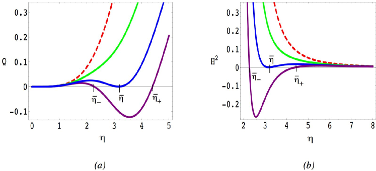
Figure 1: Numerical analysis of the radial velocity, $Q$, and the Hubble induced parameter $H^{2}$, for a brane wandering in an AdS throat geometry. We took $\alpha^{\prime}=1$, $g_{s}\,N\sim\mathcal{O}(10)$, and $\varepsilon=1$. In $(a)$ we show the evolution of $Q$ as we change the value of the angular momentum. The dashed curve corresponds to zero angular momentum. The blue line corresponds to the critical value of $l_{c}\sim 6.32$, for which there is only one root at $\bar{\eta}$. When the angular momentum is increased beyond this value this root splits into $\bar{\eta}_{\pm}$, as shown in the plot. In $(b)$ we plot the Hubble parameter induced on the brane.

In figure 1$a$ we plot the kinetic function, $Q$, for different values of the angular momentum for the case of a brane ($q=1$). When we increase the value of the angular momentum, one or two turning points arise, located at the positions given in (32). The value $\eta=0$, which corresponds to the horizon of AdS, is not a zero of $Q$ (although it is not clear from the figure!). However, when the angular momentum gets large enough, the second term in the squared root in (32) is negligible and therefore the origin becomes eventually a zero of the potential, but the brane is confined to move in the region $\eta^{2}>\bar{\eta}^{2}\sim 2\,l^{2}$.

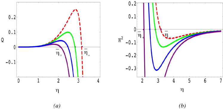
Figure 2: Numerical analysis of $Q$ and $H^{2}$ for a wandering anti-brane in an AdS throat for different values of the angular momentum. We take the same values as in the previous plot for the parameters. In $(a)$ we plot the value of $Q$ for increasing values of the angular momentum. The dashed line corresponds to zero angular momentum. In picture $(b)$ the corresponding Hubble parameter is shown.

Anti-Brane Dynamics ($q=-1$)

In the case of an antibrane, there is only one real, positive solution to (32). Thus, there is always a turning point and in fact, the antibrane can only live in the region $\eta\leq\bar{\eta}_{+}$. This region gets reduced as we increase the angular momentum, until it eventually disappears completely for very large angular momentum. In figure 2$a$ we show an explicit numerical example, for the same values of the parameters as in figure 1, for the case of an antibrane ($q=-1$).

3.2 Induced Expansion: Bouncing Universe

The induced expansion in the present simple background, is predicted from our general discussion in sections 2.1 and 2.2. The form of the induced Friedmann equation in this case is [24]

$$H^{2}_{ind}\,=\,\frac{\lambda^{1/2}}{\eta^{4}}\left[\frac{\varepsilon^{2}\lambda}{\eta^{4}}\,+2\varepsilon\,q-\frac{l^{2}}{\eta^{2}}\right]\,.$$ (36)

The induced expansion that a brane (antibrane) observer experiences, can be summarised as follows.

Moving Brane

We have seen that $Q$ has no zeros when $l=0$. Since $h^{\prime}=0$ has no solutions, we conclude that for zero angular momentum it is not possible to have a bounce. However, as the angular momentum is turned on, one or two zeros of $Q$ can arise, that is, there can be up to two turning points, $\bar{\eta}_{\pm}$. Since $H^{2}_{ind}>0$ at infinity and for small values of $\eta$, one concludes that a brane arriving from large values of $\eta$ will encounter a turning point before reaching the AdS horizon, and will bounce back [24, 37]. Since there can be two zeros, there also exists an internal region where a brane coming from the horizon will reach a given point and bounce back into the horizon. This behaviour is shown in figure 1$b$.

Moving Anti-Brane

The case of the anti-brane is slightly different. There is always one zero of $Q$, with or without angular momentum. Given that, $H^{2}_{ind}<0$ at infinity, the only possible solution is the internal bounce where the antibrane goes back to the horizon. This behaviour is shown in figure 2$b$.

Therefore, we conclude that in this simple case, the effect of the angular momentum is important to allow for a bouncing brane universe. However, a cyclic universe is clearly not possible. We will see in the next two sections that as soon as one has more complex backgrounds, the angular momentum gives the new possibility of cyclic universes.

4 Klebanov-Tseytlin Background

The first example in which the brane trajectory exhibits a cyclic behaviour is the Klebanov-Tseytlin background. This is a supersymmetric, singular solution representing the background associated with $N$ D3-branes and $M$ D5-branes wrapping a two cycle. The addition of the wrapped D5 branes modifies the warp factor with a logarithmic correction that plays a crucial role in our search for cyclic trajectories. Apart from cyclic cosmologies, we find the important feature that large enough angular momenta prevents the brane from falling into the singularity of the geometry. Although the brane can move toward the singularity, it bounces back before reaching it returning to the regular region of the geometry.

4.1 The solution

The Klebanov-Tseytlin [10] (KT) flux background describes a singular geometry produced by a number, $N$, D3-branes sourcing the self dual RR five form field strength $\tilde{F}_{5}$, and a number, $M$, D5-branes wrapping a (vanishing) 2-cycle (these are called fractional D3-branes). These branes source the RR three form field strength $F_{3}$ and there is also a nontrivial NSNS three form field $H_{3}$. The RR $C_{0}$ form and the dilaton field $\phi$ vanish for this solution. In order for our probe brane analysis to be valid, we need to have a large number of D3-branes and D5-branes. Also, in order for the supergravity description to be valid, we need to have small curvatures. These two things can be realised if we keep $g_{s}N\gg 1$, and work in the string perturbation limit $g_{s}<1$.

The complete solution takes the following form [10, 40]

$$ds^{2}_{10}=h^{-1/2}(\eta)\,dx_{\mu}dx^{\mu}+h^{1/2}(\eta)(d\eta^{2}+\eta^{2}ds^{2}_{T^{1,1}})\,.$$ (37)

Here $\eta$ is the radial coordinate of the internal six dimensional manifold, which is given by the conifold. This is a six-dimensional cone with base $T^{1,1}$, where $T^{1,1}$ is an Einstein space whose metric is

$$ds^{2}_{T^{1,1}}=\frac{1}{9}\,(g^{5})^{2}+\frac{1}{6}\,\sum_{i=1}^{4}(g^{i})^{2}\,.$$ (38)

Topologically, this is $S^{2}\times S^{3}$, and the one-form basis $\{g^{i}\}$ above is the one conventionally used in the literature, given in terms of the angular internal coordinates as:

$$g^{1,3}=\frac{e^{1}\mp e^{3}}{\sqrt{2}}\,\,,\qquad g^{2,4}=\frac{e^{2}\mp e^{4}}{\sqrt{2}}\,\,,\qquad g^{5}=e^{5}\,,$$ (39)

where,

$$e^{1}=-\sin{\theta_{1}}\,d\phi_{1}\,\,,\qquad e^{2}=d\theta_{1}\,\,,\qquad e^{3}=\cos{\psi}\,\sin{\theta_{2}}\,d\phi_{2}-\sin{\psi}\,d\theta_{2}\,,$$

$$e^{4}=\sin{\psi}\,\sin{\theta_{2}}\,d\phi_{2}+\cos{\psi}\,d\theta_{2}\,\,,\qquad e^{5}=d\psi+\cos{\theta_{1}}\,d\phi_{1}+\cos{\theta_{2}}\,d\phi_{2}\,,$$ (40)

with $0\leq\psi\leq 4\pi$, $0\leq\theta_{i}\leq\pi$, $0\leq\phi_{i}\leq 2\pi$. The $S^{2}\times S^{3}$ topology can now be readily identified as [40]

$$S^{2}:\quad\psi=0\,\,,\quad\theta_{1}=\theta_{2}\,,\quad\phi_{1}=-\phi_{2}\,\,;\qquad\quad{\rm and}\qquad\qquad S^{3}\,\,:\quad\theta_{2}\,=\,\phi_{2}=0\,.$$

The other background fields are given by [10]

$$B_{2}=\frac{3\,g_{s}\,M\,\alpha^{\prime}}{4}\,\left[\ln{\frac{\eta}{\tilde{\eta}}}\right]\,(g^{1}\wedge g^{2}+g^{3}\wedge g^{4})$$

$$H_{3}=dB_{2}=\frac{3\,g_{s}\,M\,\alpha^{\prime}}{4\,\eta}\,d\eta\wedge(g^{1}\wedge g^{2}+g^{3}\wedge g^{4})$$

$$F_{3}=\frac{M\,\alpha^{\prime}}{4}\,g^{5}\wedge(g^{1}\wedge g^{2}+g^{3}\wedge g^{4})$$

$$\tilde{F}_{5}={\mathcal{F}}_{5}+\star{\mathcal{F}}_{5}$$

$${\mathcal{F}}_{5}=B_{2}\wedge F_{3}=27\,\pi\,\alpha^{\prime 2}N_{eff}(\eta)Vol(T^{1,1})$$

$$\star{\mathcal{F}}_{5}=dC_{4}=g_{s}^{-1}d(h^{-1})\wedge dx^{0}\wedge dx^{1}\wedge dx^{2}\wedge dx^{3}$$

where the volume of $T^{1,1}$ is computed using the metric (38) and is given by $Vol(T^{1,1})=16\,\pi^{3}/27$. The functions appearing in the solution are

$$h(\eta)=\frac{27\,\pi\,\alpha^{\prime 2}}{4\,\eta^{4}}\,\left[g_{s}\,N+\frac{3\,(g_{s}\,M)^{2}}{2\pi}\,\left(\ln{\frac{\eta}{\tilde{\eta}}}+\frac{1}{4}\right)\right]=\frac{c}{\eta^{4}}\,(1+b\ln{\eta})\,,$$ (41)

$$N_{eff}=N+\frac{3\,(g_{s}M)^{2}}{2\pi}\,\ln{\frac{\eta}{\tilde{\eta}}}\,.$$ (42)

Here, $\eta=\tilde{\eta}$ determines the UV scale at which the KT throat joins to the Calabi-Yau space. This solution has a naked singularity at the point where $h(\eta_{0})=0$, located at $\eta_{0}={\tilde{\eta}}e^{-1/b}$. In this configuration, the supergravity approximation is valid when $g_{s}M,\,g_{s}N\gg 1$: in this limit the curvatures are small, and we keep $g_{s}<1$. (By taking the parameter $M=0$, one finds AdS space, without singularities.)

4.2 Brane Evolution and Physical Consequences

We are now ready to study the evolution of our probe (anti-) brane in this background. In the present solution, the Lagrangian describing this motion is given by (9) :

$${\mathcal{L}}=-m\,h^{-1}\,\left[\,\sqrt{1-h\,v^{2}}-q\right]\,.$$ (43)

The velocity of the brane in the internal space is given by

$$\dot{\eta}^{2}+\eta^{2}\left[\frac{1}{9}(\dot{g}^{5})^{2}+\frac{1}{6}\sum_{i=1}^{4}(\dot{g}^{i})^{2}\right]\,,$$ (44)

where, with a slight abuse of notation, that should not generate confusion, we have denoted

$$\dot{g}^{5}=\dot{\psi}+\cos{\theta_{1}}\dot{\phi}_{1}+\cos{\theta_{2}}\dot{\phi}_{2}$$

and similarly for the other $\dot{g}^{i}$. In general, studying the motion along all the internal coordinates is not simple, however, without loss of generality, we can concentrate on the case where the brane moves along one of the cycles of the internal manifold. In particular, let us consider motion on the $S^{3}$ cycle, defined by $\theta_{2}=\phi_{2}=0$ and take $\phi_{1}=$constant for simplicity. In this case (writing $\theta_{1}\equiv\theta$) we obtain:

$$v^{2}=\dot{\eta}^{2}+\eta^{2}\left[\frac{\dot{\psi}^{2}}{9}+\frac{\dot{\theta}^{2}}{6}\right]\,.$$ (45)

Plugging this into the Lagrangian, we see that there are two conserved angular momenta along $\psi$ and $\theta$. These are

$$l_{\psi}=\frac{\eta^{2}\dot{\psi}}{9\,\sqrt{1-h\,v^{2}}}\qquad;\qquad l_{\theta}=\frac{\eta^{2}\dot{\theta}}{6\sqrt{1-h\,v^{2}}}\,.$$ (46)

Defining the angular momentum, $l$, via

$$l^{2}\equiv 9\,l_{\psi}^{2}+6\,l_{\theta}^{2}\,,$$ (47)

gives the velocity:

$$v^{2}\,=\,\frac{\eta^{2}\dot{\eta}^{2}+l^{2}}{\eta^{2}+h\,l^{2}}\,.$$ (48)

It is clear that when $l=0$ we obtain the simple expression $v^{2}=\dot{\eta}^{2}$ and the speed limit in this case is simply $h\dot{\eta}^{2}<1$. The canonical momentum associated to $\eta$, (12), for KT is given by

$$\rho_{\eta}=\frac{\dot{\eta}}{\sqrt{1-h\,v^{2}}}\,.$$ (49)

Using this information the energy (18) takes the form,

$$\varepsilon=\frac{1}{h}\left[\sqrt{\frac{1+h\,\frac{l^{2}}{\eta^{2}}}{1-h\,\dot{\eta}^{2}}}-q\right]\,,$$ (50)

that is, an expression formally identical to the one for the motion in the $AdS_{5}\times S_{5}$ background analysed in the previous section, however, note $h$ is different. Consequently, in terms of $h$, the expression for the time derivative of $\eta$, (19), in the present case takes the familiar form:

$$\dot{\eta}^{2}=\frac{\varepsilon(\varepsilon h+2q)-l^{2}/\eta^{2}}{(h\varepsilon+q)^{2}}=Q\,\,.$$ (51)

We are interested in those regions of the space where $Q\geq 0$, therefore, we can simply look at the behaviour of

$$\varepsilon(\varepsilon\,h+2q)-\frac{l^{2}}{\eta^{2}}\geq 0\,.$$ (52)

Since $h(\eta)$ is more complicated than before, this is no longer as amenable to analytic analysis and we must proceed numerically. Of particular interest are those points where $Q=0$, where we have turning points for the brane (anti-brane). At such values, the brane typically stops and bounces. The number of zeros of (51) is obtained by looking at the solutions to

$$\varepsilon^{2}h-\frac{l^{2}}{\eta^{2}}=-2\varepsilon\,q\,,$$ (53)

which are easily obtained by looking at its asymptotic behaviour, and the form of the function $h$.

In what follows, we illustrate trajectories for a brane or anti-brane as it moves in a specific KT background, which is representative of the types of behaviour one can obtain. Figure 3 shows the warp factor $h(\eta)$ for the representative values of the parameters: $g_{s}N,\,g_{s}M\sim{\mathcal{O}}(10)$, $\alpha^{\prime}=1$. It is important to notice that this function has a zero (the location of the singularity) at the position $\eta=\eta_{0}$. Moreover, $h$ has a maximum at the point $\eta^{\prime}>\eta_{0}$, where the derivative $dh/d\eta=h^{\prime}=0$. This fact will become important in the next subsection, when we discuss the induced time dependent expansion on the brane.

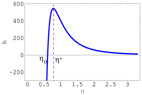
Figure 3: Plot of $h(\eta)$ given by Eq. (41). In the plot we take $\alpha^{\prime}=1$ and $g_{s}M$, $g_{s}N\sim\mathcal{O}(10)$. The point $\eta=\eta_{0}$ corresponds to the singularity, where $h$ vanishes. The maximum of $h$, is located at the point $\eta^{\prime}$, defined by $h^{\prime}(\eta^{\prime})=0$.

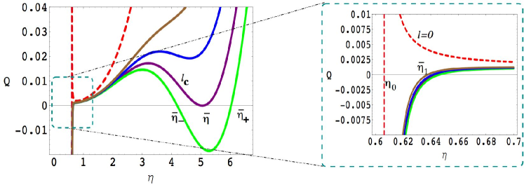
Figure 4: $Q(\eta)$ in the KT background for various angular momenta. We take $g_{s}M$, $g_{s}N\sim\mathcal{O}(10)$, $\alpha^{\prime}=\varepsilon=q=1$. The dashed line represents the value of $Q$ for zero angular momentum. The value of $l$ where a second zero of $Q$ first appears, for the choice of parameters given, is $l_{c}\sim 10.84$. The position of the first zero of $Q$, can be seen by zooming into the plot for small values of $\eta$. ¿From here, it is clear that $\eta_{0}<\bar{\eta}_{1}$, where $\eta_{0}$ is the position of the singularity, $h(\eta_{0})=0$.

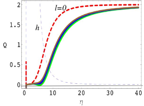
Figure 5: Large $\eta$ behaviour of $Q$ in the KT background for the same values of the parameters as in fig. (4). The thin blue line corresponds to the metric function $h$, as indicated in the figure.

Dynamics of a Brane ($q=1$)

We start our discussion with the case of a brane ($q=1$) moving in the KT background. In figure 4, we show the behaviour of $Q$ for a probe brane with fixed energy, $\varepsilon=1$, for the same values of $M$, $N$ as in figure (3). We show explicitly how $Q$, and consequently the brane trajectories, vary as we change the angular momentum. The general features of the motion of a brane with angular momentum in the KT throat are summarised as follows:

• $l=0$. For vanishing angular momentum, (51) becomes

  $$\frac{h+2}{(h+1)^{2}}=Q\,,$$ (54)

  (recall that we are taking $\varepsilon=1$). Therefore, at the singularity $\eta_{0}$ ($h=0$), and also at large $\eta$ ($h\rightarrow 0$) we have that $Q=2$. For intermediate $\eta$, the radial speed decreases to a minimum value, defined by $Q^{\prime}=0$, where $Q^{\prime}=dQ/d\eta=-h^{\prime}(h+3)/(h+1)^{3}$. There are no turning points of brane motion in this case, i.e. solutions to $Q=0$. Physically, this implies that a brane coming from the far UV region will not be able to escape from falling into the singularity of the KT geometry at some finite time, although its velocity will damp to a minimum at $\eta^{\prime}$. As we now discuss, this can be avoided by turning on angular momentum.

• $l\neq 0$. As the angular momentum is turned on, several qualitatively new phenomena can occur. First of all notice that

  $$Q=\frac{h+2-l^{2}/\eta^{2}}{(h+1)^{2}}\,,$$ (55)

  therefore at the singularity $Q(\eta_{0})=2-l^{2}/\eta_{0}^{2}$. It is clear that as soon as we take, $l^{2}>l^{2}_{min}=2\,\eta_{0}^{2}$,    $Q(\eta_{0})<0$ at the singularity, hence the singularity is now in a kinetically forbidden region. On the other hand, since $Q\to 2$ for large values of $\eta$, independent of the angular momentum (see fig. 5), we conclude that $Q$ has to cross zero at least once between the singularity and infinity. In other words, for generic values of the angular momentum, there is at least one point, $\bar{\eta}_{1}>\eta_{0}$, where the radial brane speed becomes zero, $Q=0$. Therefore, a brane coming from the UV region will bounce back before reaching the singularity.

  The points where the radial brane speed vanishes are determined by the equation

  $$G(\eta)=2{\eta^{4}}-{l^{2}}{\eta^{2}}+c(1+b\,\ln{\eta})=0\,.$$ (56)

  This equation can have a maximum of three (real positive) zeros. The position and number of such zeros depends on the value of the angular momentum.

  We can thus have three different situations, depending on the value of the angular momentum. Let $l_{c}$ be the value of the angular momentum for which an additional zero of (56) appears. For $l<l_{c}$, there is only one zero at $\bar{\eta}_{1}$, say. For $l>l_{c}$, the second zero $\bar{\eta}$ resolves into two different zeros, $\bar{\eta}_{\pm}$ say, and we end up with three zeros. The presence of these turning points is quite interesting as it allows for a variety of new trajectories that the brane can follow. Also, note that the singularity of KT is avoided for all these trajectories. These behaviours are important for the induced expansion, allowing for novel bouncing and cyclic universes. We now turn to a discussion of the brane physics for these values of the angular momentum.

  • $l_{min}<l<l_{c}$. In this case, a D3-brane falling into the KT throat decelerates more rapidly than if it had no angular momentum, and eventually slingshots at $\eta=\bar{\eta}_{1}$, rebounding back up the throat, without ever reaching the singularity.

  • $l=l_{c}$. In this case, a new zero for the radial speed arises at $\bar{\eta}=\bar{\eta}_{+}=\bar{\eta}_{-}$. Therefore, a brane coming down the throat asymptotes a steady orbit at that point. Moreover, a new kind of trajectory is possible. A brane can actually be in orbit (at $\bar{\eta}$) around the KT singularity and fall in towards the conifold tip, rebound and asymptote its original orbit.

  • $l>l_{c}$. For larger values of the angular momentum, there are two separate physical regions for the brane motion. For the region $\eta>\bar{\eta}_{+}$, the brane descends through the throat, from large to small values of $\eta$, slingshotting at $\bar{\eta}_{+}$, and rebounding back toward large values of $\eta$. On the other hand, in the region $\bar{\eta}_{1}<\eta<\bar{\eta}_{-}$, a bound state arises, corresponding to the brane oscillating between these two turning points (see fig. 4). The presence of these turning points will be very important for the induced expansion analysis in the next section, as it gives rise to cyclic universes.

Dynamics of Anti-Branes ($q=-1$)

Let us now move on to the case of an anti-brane moving along the KT throat. This is, in some way, simpler than the brane case, as we now see. We show this example numerically in figure 6$a$, for the same values for the parameters as in figures 3–5.

• $l=0$. When no angular momentum is present, $Q=(h-2)/(h-1)^{2}$. Therefore, this quantity has a singularity at the two points where $h=1$. When $1<h<2$, $Q<0$, and therefore this region is kinetically forbidden. When $h>2$, $Q$ becomes positive, however, for large values of $\eta$, it becomes negative (unphysical) again, as $Q\to-2$. It is clear that $Q=0$ has two zeros, corresponding to turning points of the motion, at the positions where $h=2$. The precise location of these is determined by the equation,

  $$\frac{c}{\eta^{4}}\,(1+b\,\ln{\eta})=2$$ (57)

  and we call $\bar{\eta}_{\pm}$ the positions of these zeros. Of course, the regions beyond the greatest zero of the equation above are unphysical as $Q<0$. Therefore, an antibrane moving in this background will never have enough energy to escape the “gravitational attraction” due to the geometry, and will stay in a bound state, bouncing back and forth between the radii $\bar{\eta}_{-}<\eta<\bar{\eta}_{+}$, without ever reaching the singularity. In figure 6$a$, the zero momentum case is shown in dashed lines.

• $l\neq 0$. The qualitative behaviour of the anti-D3-brane trajectories when the angular momentum is turned on is the same as in the zero momentum case. This can be easily understood since the number of zeros of $Q$ stays the same, although the location changes, according to the equation

  $$\frac{c}{\eta^{4}}\,(1+b\,\ln{\eta})-\frac{l^{2}}{\eta^{2}}=2\,.$$ (58)

  In figure 6$a$, we show how the position of these two zeros changes as we increase the value of the angular momentum. Therefore, the trajectories of the antibrane are as before: An anti-brane wandering in the throat of KT, is always constrained to stay near the throat, oscillating between the two zeros of $Q$. As we will see in the next section, this behaviour will be reflected in a cyclic kind of expansion, when seen from the antibrane observer’s point of view.

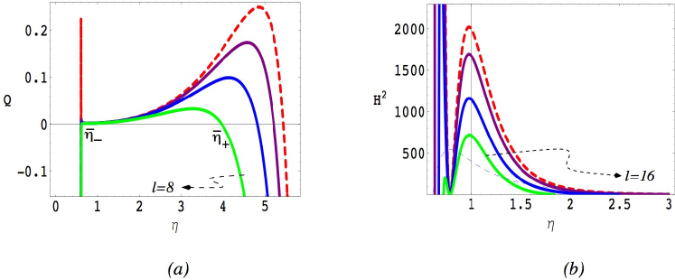
Figure 6: Variation of $Q$, $(a)$, and $H^{2}$, $(b)$, for the case of an anti-brane moving in the KT background. In this case, even for $l=0$, the quantity $Q$ has two roots, $\bar{\eta}_{\pm}$. When the angular momentum is added, the physical region where $Q>0$ diminishes, till it eventually disappears. Notice that for $\eta>\eta_{+}$, where $\eta_{+}$ is the biggest root of $Q$, there is no physical region. In terms of the Hubble induced expansion, these two roots give only cyclic universes for an antibrane.

4.3 Induced Expansion in KT: Cyclic/Bouncing Universe

The induced expansion that a brane (antibrane) observer experiences as they move in the KT background provides novel examples of bouncing and, more interestingly, cyclic brane universes, as we show below. For the KT background, eq. (28) becomes

$$H_{ind}^{2}=\left(\frac{h^{\prime}}{4\,h^{3/4}}\right)^{2}\left[\varepsilon\,(h\,\varepsilon+2q)-\frac{l^{2}}{\eta^{2}}\right]=\left(\frac{h^{\prime}}{4\,h^{3/4}}\right)^{2}(h\,\varepsilon+q)^{2}\,Q\,.$$ (59)

As we already mentioned, the angular momentum provides a negative contribution that can be compared to a positive curvature contribution in the standard FRW cosmology, thus, one can expect to get bounces once it is nonzero. In fact, the behaviour is far more interesting. In what follows, we discuss the generic behaviour of a brane/anti-brane moving in this background and illustrate it with several pictures.

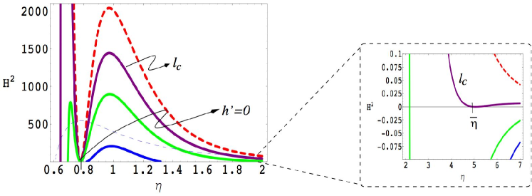
Figure 7: Plot of $H^{2}(\eta)$ given by (59) for a brane. In the plot we take the same values for the parameters as in figure 4. The dashed curve corresponds to zero angular momentum, whereas the purple corresponds, as indicated, to $l_{c}$. The value of $\bar{\eta}$, where $Q=0$ for this curve (see figure 4), is shown by zooming in on the curves around that point. The point at which $h^{\prime}=0$ is $\eta^{\prime}\sim 0.8$. The green curve corresponds to $l=19$. For this value of the angular momentum, the three first zeros of $H^{2}$ are clearly seen. The fourth lies outside the region shown in the plot.

Brane Expansion ($q=1$)

We now analyze the case of a moving brane. The type of induced expansion that a brane observer will experience is inferred from our previous discussion on the brane dynamics. We describe each case in detail and again we illustrate our results graphically with a numerical example. For the brane, the behaviour is graphically depicted in figure 7.

• $l=0$. As we saw in the previous section, the quantity $Q$ is always positive and has no zeros. However, it is still possible for the cosmological expansion to experience a bounce if $h^{\prime}=0$. This happens at only one value of $\eta$, $\eta^{\prime}$, where $h$ has a maximum (see fig. 3). Therefore, a brane observer actually experiences a contracting Universe, as the brane falls towards $\eta^{\prime}$, which then bounces and re-expands, and in fact hyperinflates toward a final cosmological singularity in finite time.

• $l\neq 0$. In this case, $Q$ can have up to three different roots, depending on the values of $l$. Since $h^{\prime}$ has a zero at $\eta^{\prime}$, the induced Hubble parameter (59) can have a maximum of four zeros, giving rise to a rich structure. We consider each case separately.

  • $l_{min}<l<l_{c}$. In this case, $H^{2}$ has two zeros. One is located at $\eta^{\prime}$ and the other at $\bar{\eta}_{1}$ (one can check that $\bar{\eta}_{1}<\eta^{\prime}$). This is also clear from the plot of $H^{2}$ in figure 7. Therefore, a brane coming down the throat, will experience a contracting phase moving to an expanding phase at $\eta^{\prime}$ and then enter another contracting phase at $\bar{\eta}_{1}$, expanding again at $\eta^{\prime}$.

  • $l=l_{c}$. As we increase the angular momentum to the critical value where $Q$ has two roots, a new zero for $H^{2}$ arises. Thus there are three turning points where $H^{2}=0$. In figure 7, we zoom into the region where the zero of $Q$ at $\bar{\eta}$ appears. As we have already remarked, these are two possible brane trajectories. The first corresponds to a contracting phase (as the brane moves in from the UV) asymptoting a steady-state Universe orbiting at $\eta=\bar{\eta}$. The other corresponds to a bouncing Universe, oscillating between contracting and expanding phases.

  • $l>l_{c}$. In this case, there are four turning points, where $H^{2}=0$. This gives rise, inevitably, to cyclic universes. A brane coming from values of $\eta>\bar{\eta}_{+}$, will reach the turning point and bounce back to the UV region corresponding to a contracting/expanding cosmology. However, a brane moving in the region $\bar{\eta}_{1}<\eta<\bar{\eta}_{-}$ will experience a multi-cyclic expansion. In figure 8 we plot $H^{2}$ for $l=15$ where the typical behaviour of the brane evolution along the throat is clearer.

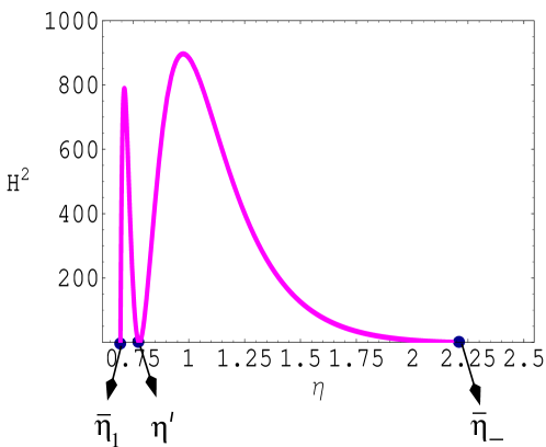
Figure 8: Plot of $H^{2}(\eta)$ for $l=15$. The position of the three first zeros of $H^{2}$ are shown. The two associated cyclic universe regions are shown clearly.

Anti-Brane Expansion ($q=-1$)

The situation in the case of a wandering anti-brane is very simple to understand from the analysis of the trajectories discussed in the last section. $Q$ has two roots, or turning points, independent of the value of the angular momentum, which disappear as $l$ becomes too large. Therefore, the induced expansion in this case has the same qualitative form for $l=0$ and $l\neq 0$. The form of the Hubble parameter for the antibrane is shown in figure 6$b$.

As with the brane, there is another solution to $H^{2}=0$ coming from $h^{\prime}=0$. Therefore, $H^{2}$ has a total of 3 zeros, or turning points, as can be seen from figure 6$b$. Since $H^{2}$ becomes negative after we reach the (biggest) solution of $h=2$ ($Q=0$) at $\bar{\eta}_{+}$, then, an antibrane observer will always experience a cyclic expansion, moving, as in the case of the brane, between the two solutions of $Q=0$, without touching the singularity.

5 Klebanov-Strassler Background

The last background we study in detail is given by the Klebanov-Strassler geometry, a regularised version of the KT throat studied in the previous section based on the deformed conifold. The metric ansatz for this background is slightly more complicated than in the previous case, allowing for differential warping of the angular coordinates. The brane trajectories are also rich, exhibiting bouncing and cyclic behaviour, depending on the brane energy and angular momenta.

5.1 The solution

We now consider the regularisation of the KT solution due to Klebanov and Strassler (KS) [11]. It describes the geometry due to a configuration of (a large number) $N$ D3-branes and (a large number) $M$ wrapped D5-branes. A cartoon of the regularisation of the KT solution is shown in figure 9.

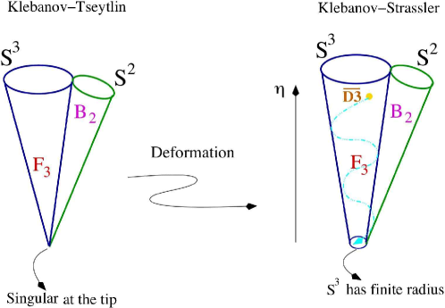
Figure 9: Cartoon representation of the KS resolution of the KT singular background.

The metric and the other fields are given by

$$ds^{2}_{10}=h^{-1/2}(\eta)\,dx_{\mu}dx^{\mu}+h^{1/2}(\eta)ds^{2}_{6}\,,$$ (60)

where the 6D metric is now replaced by that of the deformed conifold (see ref. [39])

$$ds^{2}_{6} = \frac{\epsilon^{4/3}}{2}\,K(\eta)\Bigg{[}\frac{1}{3\,K(\eta)^{3}}\,\left\{d\eta^{2}+(g^{5})^{2}\right\}$$ (61)

$$\hskip 28.45274pt+\cosh^{2}{(\eta/2)}\left\{(g^{3})^{2}+(g^{4})^{2}\right\}+\sinh^{2}{(\eta/2)}\left\{(g^{1})^{2}+(g^{2})^{2}\right\}\Bigg{]}\,,$$

where the $\{g^{i}\}$ basis is defined as before and $\epsilon$ is a constant that measures the deformation of the conifold. The other fields are given by

$$B_{2}=\frac{g_{s}\,M\,\alpha^{\prime}}{2}\,\left[f(\eta)\,g^{1}\wedge g^{2}+k(\eta)\,g^{3}\wedge g^{4}\right]\,,$$

$$H_{3}=\frac{g_{s}\,M\,\alpha^{\prime}}{2}\,\left[d\eta\wedge(f^{\prime}(\eta)\,g^{1}\wedge g^{2}+k^{\prime}(\eta)\,g^{3}\wedge g^{4})+\frac{1}{2}\left(k(\eta)-f(\eta)\right)g^{5}\wedge\left(g^{1}\wedge g^{3}+g^{2}\wedge g^{4}\right)\right]\,,$$

$$F_{3}=\frac{M\,\alpha^{\prime}}{2}\,\left[\left(1-F(\eta)\right)g^{5}\wedge g^{3}\wedge g^{4}+F(\eta)\,g^{5}\wedge g^{1}\wedge g^{2}+F^{\prime}(\eta)\,d\eta\wedge\left(g^{1}\wedge g^{3}+g^{2}\wedge g^{4}\right)\right]\,,$$

$$\tilde{F}_{5}={\mathcal{F}}_{5}+\star{\mathcal{F}}_{5}=B_{2}\wedge F_{3}+dC_{4}$$

$$dC_{4}=g_{s}^{-1}d(h^{-1})\wedge dx^{0}\wedge dx^{1}\wedge dx^{2}\wedge dx^{3}\,.$$

Again, the dilaton and the RR zero form vanish in this solution. The explicit form of the functions appearing above is:

$$F(\eta)=\frac{\sinh{\eta}-\eta}{2\sinh{\eta}}\,,$$ (62)

$$f(\eta)=\frac{\eta\,\coth{\eta}-1}{2\sinh{\eta}}(\cosh{\eta}-1)\,,$$ (63)

$$k(\eta)=\frac{\eta\,\coth{\eta}-1}{2\sinh{\eta}}(\cosh{\eta}+1)\,,$$ (64)

$$K(\eta)=\frac{\left(\sinh{(2\,\eta)-2\,\eta}\right)^{1/3}}{2^{1/3}\,\sinh{\eta}}\,,$$ (65)

$$h(\eta)=(g_{s}M\alpha^{\prime})^{2}2^{2/3}\,\epsilon^{-8/3}\int_{\eta}^{\infty}{dx\,\frac{x\,\coth{x}-1}{\sinh^{2}{x}}\,\left(\sinh{(2\,x)-2\,x}\right)^{1/3}}\,.$$ (66)

Although the integral above, conventionally denoted as $I(\eta)$, cannot be computed analytically, one can readily work out the two important limits of the solution as $\eta\to 0$ and $\eta\to\infty$, [11, 40]. One can check that near the bottom of the throat (IR), the internal metric takes the form of a 3-sphere with finite radius, plus a 2-sphere which shrinks to zero size. At the other end of the throat (UV), the metric takes the form of the KT solution, asymptoting AdS spacetime. The relevant limits of the integral above are

$$I(\eta\to 0)\to a_{0}+{\mathcal{O}}(\eta^{2})\,\,;\qquad I(\eta\to\infty)\to 3\cdot 2^{-1/3}(\eta-1/4)\,e^{-4\eta/3}\,,$$ (67)

where $a_{0}=0.71805$ [40].

5.2 Brane Evolution and Physical Consequences

We are again dealing with a the Lagrangian of the form (9) and we take the brane to be moving along the same cycle as in KT. Therefore the speed in the present case becomes ($\theta_{1}=\theta$):

$$v^{2}=A(\eta)\,\left[\dot{\eta}^{2}+\dot{\psi}^{2}\right]+B(\eta)\,\dot{\theta}^{2}$$ (68)

where

$$A(\eta)=\frac{\epsilon^{4/3}}{6K^{2}}\,,\qquad\quad B(\eta)=\frac{\epsilon^{4/3}K}{4}\,\left[\cosh^{2}{(\eta/2)}+\sinh^{2}{(\eta/2)}\right]$$ (69)

The two conserved angular momenta along $\psi$ and $\theta$ are given by

$$l_{\psi}=\frac{A\,\dot{\psi}}{\sqrt{1-h\,v^{2}}}\,;\qquad\qquad l_{\theta}=\frac{B\,\dot{\theta}}{\sqrt{1-h\,v^{2}}}\,,$$ (70)

and the canonical momentum associated to $\eta$ is

$$\rho_{\eta}=\frac{A\,\dot{\eta}}{\sqrt{1-h\,v^{2}}}\,.$$ (71)

Using this information, the energy (18), becomes

$$\varepsilon=\frac{1}{h}\left[\sqrt{\frac{1+h\,\ell^{2}(\eta)}{1-h\,g_{\eta\eta}\,\dot{\eta}^{2}}}-q\right]$$ (72)

where

$$\ell^{2}(\eta)=\frac{l_{\psi}^{2}}{A}+\frac{l_{\theta}^{2}}{B}\,.$$ (73)

The time evolution of the brane along the radial coordinate $\eta$ (19) is then determined by

$$\dot{\eta}^{2}=\frac{\left[\varepsilon(h\,\varepsilon+2q)-\ell^{2}(\eta)\right]}{A(h\,\varepsilon+q)^{2}}=Q\,.$$ (74)

We now study the behaviour of the brane (or anti-brane), as it moves in this background. We find that, although the motion has many similarities with the KT case, there are some important differences.

Dynamics of a brane ($q=1$)

In order to study the form of the brane trajectories in the KS background, we numerically evaluate the metric function (66) for consistent values of the parameters. We take $\alpha^{\prime}=1$ and $g_{s}M$, $g_{s}N\sim\mathcal{O}(10)$, and plot the relevant metric functions in figure 10. Moreover, note the presence of a $g_{\eta\eta}=A(\eta)$, and the effect of the differential warping $A(\eta)$ and $B(\eta)$. Although these functions become proportional at large $\eta$ ($B\propto 3A/4$), their precise form at finite values of $\eta$, will be important when we turn on the angular momenta $l_{i}$. Notice that, in contrast with the KT case, $h>0$ for all values of $\eta$, and tends to zero for large values of $\eta$ only. This will have important consequences later. Let us look in more detail at the brane evolution in the KS background. We concentrate on the case $\varepsilon=1$, and show the results for $Q$ as we change the angular momenta in figure 11.

• $l_{i}=0$. When both momenta are zero, $Q$ becomes

  $$Q=\frac{h+2}{A(h+1)^{2}}\,.$$

  Therefore, at $\eta=0$, it has a constant positive value, $Q_{0}=Q(0)$. Since $h\,,A>0$, in this case, $Q>0$ for all $\eta$ values. Therefore a D3-brane is free to move along the entire geometry without restrictions. It will do so by increasing its radial velocity as it moves toward the tip of the throat, but decreasing it as it comes closer to it (see fig. 11).

• $l_{i}\neq 0$. As we turn on the angular momentum, the brane’s radial speed decreases relative to no angular contribution, eventually reaching a zero value for large enough angular momenta. The turning points where this can happen, are given by the equation

  $$h-\ell^{2}(\eta)=-2\,.$$

  Just as in the case of the KT background, one can check that the maximum number of solutions for this equation is three. In particular, it is the contribution of $l_{\theta}$ that provides a third solution. This can be seen from figure 11. Therefore, without loss of generality, we can extract the most general type of trajectories by concentrating on the case $l_{\psi}=0$, $l_{\theta}\neq 0$. The behaviour is very similar to the KT one, with some interesting differences, which we now describe.

  • $l_{\theta}<l_{c}$. In this case, there are no solutions to $Q=0$, thus, the trajectories are qualitatively the same as in the zero momentum case, the only difference being that the radial speed decreases via a centrifugal repulsion.

  • $l_{\theta}=l_{c}$. At this point, the equation $Q=0$ has a solution at $\bar{\eta}$, where the radial speed and acceleration vanishes. A brane coming from the UV region, will asymptote a circular orbit at $\bar{\eta}$.

  • $l_{\theta}>l_{c}$. When the angular momentum is increased above the critical value, three turning points can appear at $\bar{\eta}_{1}$, $\bar{\eta}_{\pm}$, as shown in figure 11$b$. Therefore, there are two separate regions where the brane can move. For values of $\eta>\bar{\eta}_{+}$ the brane coming down the throat, will reach a maximum distance from the tip, where its radial speed is zero, bouncing back to the region of large $\eta$ values. Moreover, a new internal region appears between, $\bar{\eta}_{1}<\eta<\bar{\eta}_{-}$, where the brane motion is bounded, as shown in figure 11.

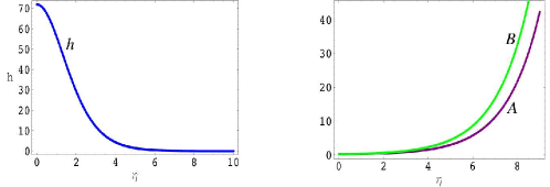
Figure 10: Plot of $h(\eta)$ given by Eq. (66), and functions $A$ and $B$. In the plot we take $\alpha^{\prime}=1$ and $g_{s}M$, $g_{s}N\sim\mathcal{O}(10)$.

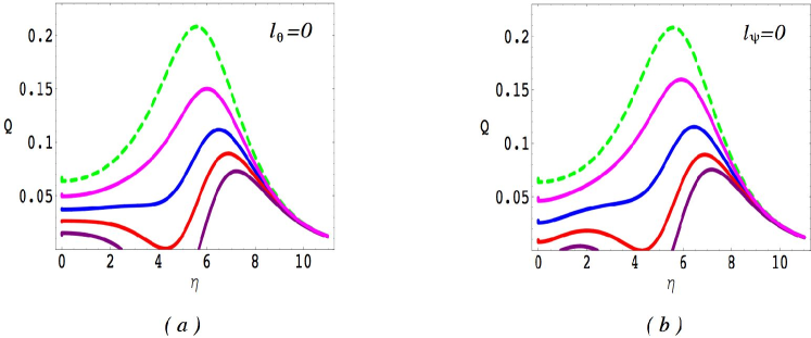
Figure 11: The function $Q$ for a brane moving in the KS background as the angular momenta changes. In picture $(a)$ we keep $l_{\theta}=0$, and allow $l_{\psi}$ to vary, whereas in $(b)$ we keep $l_{\psi}=0$ and change $l_{\theta}$. It is clear that in the second case, a second zero can appear near the tip of the deformed conifold. We took the same values for the parameters as in figure 10 and $\varepsilon=1$.

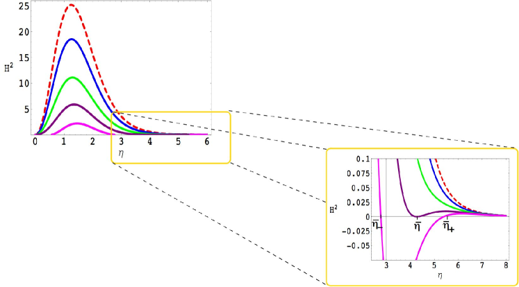
Figure 12: Induced expansion as seen by a brane observer when the brane moves along the KS throat. The parameters are chosen as in figure 3. There is always a zero of $H$ at the origin of the regular KS geometry. We zoom in on the right region where it is clear that the zeros of $Q$ are located, as we increase the angular momentum. As explained in the text, for $l_{\theta}>l_{c}$ there are no zeros for $H$ apart from the origin. For $l_{\theta}=l_{c}$ a new zero arises, at $\bar{\eta}$. This zero splits into $\bar{\eta}_{\pm}$ as we increase $l$ above its critical value. For the values of the parameters we are taking on the plot, $l_{c}\sim 3.764$.

Dynamics of an Anti-Brane ($q=1$)

The case of an antibrane wandering in the KS throat is very similar to the case of the KT background. The trajectories of the antibrane behave very similarly, independent of the value of the angular momentum. There is however, a small range of parameters, where a small variation can arise. Let us now study the trajectories in detail. We concentrate, as in the previous case, only on the case where $l_{\psi}=0$, since, as we explained above, it is $l_{\theta}$ which provides the rich structure of the trajectories.

• $l_{i}=0$. When the angular momenta vanishes, there is a single solution to $Q=0$, that is, $h=2$, at $\bar{\eta}$, say, as can be seen by the form of $h$ (fig. 10). Therefore, the antibrane is constrained to move in the region between the resolved tip of the conifold, and $\bar{\eta}$. This case is represented in figure 13$a$ by the dashed line. One can compare this to the KT case in figure 6$a$.

• $l_{\theta}\neq 0$. When the angular momentum is turned on, the equation $Q=0$ implies

  $$h-\frac{l_{\theta}^{2}}{B}=2\,.$$

  Given the form of $h$ and $B$, one can easily check that, for generic values of the angular momentum, there is always one solution, just as in the previous case. However, the position of the zero of the radial speed shifts to smaller values of $\eta$, restricting the region of solutions for the antibrane trajectories. Also, the value of the radial speed decreases (see fig. 13$a$). As we increase the value of the angular momentum, the radial speed continues to decrease, until, the region where the antibrane can move, vanishes. As this happens, there is a small range of values of $l_{\theta}$ where a bounded state with small radial speed arises. This happens when the solution to the equation above has two solutions $\bar{\eta}_{\pm}$. This region will become clearer when we look at the induced expansion in the next subsection. In figure 13$a$ we show how the antibrane radial speed changes with the angular momentum ($l_{\theta}$).

5.3 Induced Expansion in KS: Cyclic/Bouncing Universe

The induced expansion that a brane (antibrane) observer experiences in the present case, can be already intuited using our experience with the AdS and the KT backgrounds. Using (19) and (28) in the KS case, we find the effective 4D Friedmann equation:

$$H^{2}_{ind}=\left(\frac{h^{\prime}}{4\,h^{3/4}}\right)^{2}\left[\frac{\varepsilon\,(h\,\varepsilon+2q)}{A}-\frac{l_{\psi}^{2}}{A^{2}}-\frac{l_{\theta}^{2}}{A\,B}\right]=\left(\frac{h^{\prime}}{4\,h^{3/4}}\right)^{2}(\varepsilon\,h+q)^{2}\,Q$$ (75)

Therefore, just as in the previous two examples (AdS and KT) the angular momentum provides an important negative contribution to the Friedmann effective equation which again gives rise to bouncing and cyclic universes. We now consider these solutions in detail and, as in the previous analysis, we compute numerically a concrete example, which illustrates our results.

Moving Brane

We start with the case of a brane ($q=1$). The generic behaviour is very similar to the KT case. The main difference is that there is no singularity in the background, and the form of $h$, and thus $h^{\prime}$ changes. We show this case in figure 12.

• $l_{i}=0$. The vanishing momentum case is shown with a dashed line in figure 7. Following our general analysis in section 2.2, we know that in order to get bounces, there should be solutions to $H^{2}_{ind}=0$. For vanishing angular momentum, these solutions are provided by $h^{\prime}=0$. In the KS case, this has a single solution at $\eta=0$. Therefore, there is a single zero for the induced Friedmann equation. Physically, a brane coming from the UV region of the KS background, arrives at the end of the throat at $\eta=0$, where it passes through, returning to the UV region along an antipodal direction. This solution was studied in [29].

• $l_{i}\neq 0$. When the angular momentum is turned on, there is a maximum of three zeros for $Q=0$ at $\eta\neq 0$. Besides these, there is the extra zero of $h^{\prime}$ at $\eta=0$. Thus, (75) has a maximum of four zeros, which represent bouncing points for the induced cosmology. As can be seen from figure 12, there are three different situations, depending on the amount of angular momentum, with similar behaviour to the KT case.

  • $l_{\theta}<l_{c}$. For these values of the angular momentum, the situation is the same as for the case of no angular momentum, that is the brane experiences a single bounce at the origin, with $H^{2}$ reduced relative to $l=0$.

  • $l_{\theta}=l_{c}$. When $Q$ has a single zero at $\bar{\eta}$, the universe once more asymptotes a steady state cosmology in orbit at $\eta=\bar{\eta}$.

  • $l_{\theta}>l_{c}$. For larger values of $l_{i}$, there are four solutions to $H^{2}=0$: $0$, $\bar{\eta}_{1}$, $\bar{\eta}_{\pm}$. Then, two different regions for the brane expansion appear. The brane observer can either experience a bounce at the largest zero of $Q=0$, $\eta=\bar{\eta}_{+}$, or it can bounce back and forth, between the two smaller zeros of $Q=0$, $\bar{\eta}_{1}\leq\eta\leq\bar{\eta}_{-}$. Therefore a brane observer will experience a cyclic expansion. (Note that the region between $0<\eta<\bar{\eta}_{1}$ is not physical.)

Moving Anti-Brane

The case of an antibrane ($q=-1$) moving in the KS background may be anticipated from our previous analysis of AdS and KT backgrounds. Indeed the physical behaviour changes only slightly. We illustrate our results in figure 13$b$. One can compare this picture with that of the KT background, figure 6.

• $l_{i}=0$. For vanishing $l_{i}$, we saw that $Q=0$ has always a single solution. Therefore, $H^{2}=0$ has two solutions. Physically, an antibrane will always experience a cyclic expansion, bouncing back and forth between zero (where $h^{\prime}=0$) and the single root of $Q$ at $\bar{\eta}$.

• $l_{\theta}\neq 0$. As we turn on the angular momentum, in general, the trajectories have the same qualitative behaviour as before. That is, the antibrane experiences a cyclic expansion. The effect of the angular momentum is to decrease the value of the Hubble parameter induced on the brane, until the region where $H^{2}>0$ vanishes. Before this happens, there is a small region of values of the angular momentum, where two roots of $Q$ appear at $\bar{\eta}_{\pm}$, as we saw before. In those cases, the cyclic brane universe exists between these two roots of $Q$, and the region between $\eta=0$ and the smaller root of $Q$ is not physical.

As it is clear from our discussion, cyclic behaviour is quite generic, once we turn on angular momentum.

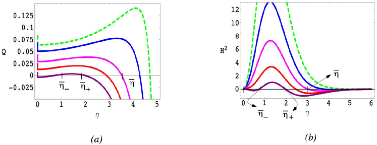
Figure 13: The anti-brane kinetic function $Q$ ($a$) and Hubble induced expansion $H^{2}$ $(b)$, for the same values of parameters as in figs. 10–12, as the angular momentum $l_{\theta}$ changes. In both pictures, the dashed line corresponds to vanishing angular momentum. The value of the angular momentum for which a new zero of $H$ arises, for the values we are taking is $l_{\theta}\sim 4.02$.

6 Discussion

In this paper, we studied in detail the dynamics of probe D3-branes and antibranes, as they move along the transverse directions of a warped supergravity background with fluxes. In particular, we allowed the brane (antibrane) to move in more than one of the transverse internal coordinates: that is, along angular as well as radial coordinates. In so doing, we have uncovered interesting novel trajectories that a brane/antibrane can take in these backgrounds.

We began by considering the pure $AdS_{5}\times S_{5}$ geometry as a classic and well known example. This has been analysed in the literature for the case of a moving brane, and we have completed the picture by including the antibrane. We then modified the background with the addition of fluxes, considering respectively the Klebanov-Tseytlin and Klebanov-Strassler backgrounds. Not surprisingly, the dynamics of the brane on these three backgrounds presents some similarities, due to the fact that the warping has similar features in all the three examples. However, a more careful study revealed interesting differences. These differences are related both to the varying forms of the warp factors in the three cases, and to the different manifolds in which the angular coordinates are compactified. For a probe brane in the three examples, we found that the type of trajectories depend crucially on the value of the angular momentum.

It is possible to distinguish between three qualitatively different possibilities for the brane dynamics. In the first case, the brane moves freely through the whole spacetime, eventually reaching the tip of the throat (either the AdS horizon, the singularity or the regularised tip). In the second case, a brane coming from the UV experiences a bounce that brings it back and does not allow it to approach the tip of the throat. This case is interesting because it shows that a brane that moves through singular backgrounds, like the KT, can have regular trajectories that avoid the singular parts of the geometry. In the last case, the brane is confined to move inside a bounded region, providing a novel example of cyclic motion inside the throat. For a probe antibrane, the trajectories are qualitatively independent of the value of the angular momentum in the three examples that we considered. In the KT and KS geometries, a turning point occurs before the tip of the throat.

We also studied the brane evolution as seen from the point of view of a brane observer, or mirage cosmology [24]. The trajectories found suggested the possibility of both bouncing and cyclic universes. Indeed, for the pure AdS throat, as was shown in [24, 37] for branes, bouncing universes arise naturally as we turn on the angular momentum, whereas they are always present for the antibrane.

More interesting are the KT and KS backgrounds where a bouncing universe is always present. This, as we pointed out in the text, is due to the form of the warp factor. When we turn on the angular momentum, as well as bouncing, cyclic cosmologies also arise. Although we have studied three specific backgrounds, we expect the same qualitative behaviour in a generic warped compactification. One of the nice features about having cyclic trajectories is that, whether or not they correspond in the final analysis to cyclic universes (which depends on the effect of backreaction), the brane experiences successive periods of acceleration during this motion, which can feed into successive inflationary eras [18].

Our analysis can be extended in several directions, for example, we have not taken into account any mechanism for the stabilization of the Kähler moduli, and the consequences of this for the action of the probe brane. This is an important issue for any genuine cosmological brane scenario in which we would require stabilization of all moduli. Initial work, [32], indicates that the effect of stabilization is to cause an additional attractive force towards the tip of the KS throat. Presumably, this will lift the critical values of angular momentum for which there is sufficient centrifugal repulsion for a bounce in the throat to occur. We do not expect the qualitative families of trajectories to be altered however. In particular, we would still expect cyclic trajectories in the stabilized KS throat.

More importantly, we have neglected the gravitational backreaction of the probe brane in our discussion of cosmology, in other words, we have been taking the mirage point of view. Although this is one possible way to proceed, it may not be the most satisfactory one. In the case of a simple codimension one braneworld, such as Randall-Sundrum, the association between moving branes and cosmology is proven. Because of the symmetry of the geometry, and hence equations of motion, any isotropic perfect fluid cosmological source can be added to the brane and fully supported as a solution to the equations of motion via the Israel equations. However, we already lose this concrete correspondence as soon as we add one more dimension, even within the supergravity description which, as we have discussed, is severely limited for the probe brane. Thus, for codimension two and higher, there is no prescriptive way to add energy momentum to a brane. Given this, it is difficult to get a concrete formulation of any mirage description as truly corresponding to a cosmological universe containing real matter, and evolving according to local physical principles. In fact, the ‘matter’ in the mirage scenario is simply that inferred from applying the standard Einstein-FRW equations to the induced evolution, and is not the result of any localised fields on the brane. It is difficult to see how to address problems such as reheating, particle production, or indeed whether we can get a sensible description of the standard model on a probe brane.

For this reason, we have discussed the induced cosmology of our brane trajectories in a somewhat limited fashion, as we do not believe that computation of properties depending on a particle interpretation (such as the spectral index of perturbations) will be robust to any mechanism for embedding this interpretation into a more complete gravitational description. As we have remarked, it appears that it is not possible within the supergravity approximation to get a truly gravitational description of a moving brane with matter in more than one codimension (although, see [41] for progress in the case of Gauss-Bonnet gravity), and given that one of the important novel cosmological predictions of the Randall-Sundrum model was the addition of $\rho^{2}$ terms to the Friedman equation, the lack of a rigorous means to project gravity onto the brane is disappointing from the point of view of a spacetime picture of string cosmology. However, one can take a more pragmatic approach to backreaction, and as a first step couple the DBI action we have studied to four dimensional gravity along the lines of [42], and analyse the resulting cosmologies as in [18]. A full study of cosmology in this direction is currently underway.

Of particular cosmological relevance is whether the cycling trajectories we have found in this paper will correspond to cyclic universes in the gravitationally coupled theory. In fact it is straightforward to show that this is not the case. Computing $\rho$ and $p$ from the Lagrangian (9), even allowing for a possible potential term for the radial variable, demonstrates that the energy momentum obeys both the weak and null energy conditions, and hence a cyclic evolution of the scale factor cannot arise. Note that this does not mean that the brane cannot follow a cycling trajectory in the throat, simply that this cycling trajectory cannot correspond to a cyclic universe. The addition of the effective Einstein Hilbert term on the brane breaks the direct correspondence between the scale factor of the four-dimensional cosmology and the radial position function of the brane. Because of this, it is possible that a brane could have an epoch of cycling in the throat, before exiting into the asymptotic regime and standard big bang cosmology. It is interesting that this simple first step towards gravitational back reaction gives such a radical modification of the mirage picture, however, it is always possible that higher order corrections may negate this.

Finally, another interesting issue related to our results is the dual field theory interpretation of the cycling trajectories: this could provide further intriguing connections between cosmological trajectories and their interpretation in the dual theory.