ITEP/TH-01/07

On the shapes of elementary domains or

why Mandelbrot Set is made from almost ideal circles?

V.Dolotin and A.Morozov

ITEP, Moscow, Russia

ABSTRACT

Direct look at the celebrated ”chaotic” Mandelbrot Set in Fig..1 immediately reveals that it is a collection of almost ideal circles and cardioids, unified in a specific forest structure. In /hep-th/9501235 a systematic algebro-geometric approach was developed to the study of generic Mandelbrot sets, but emergency of nearly ideal circles in the special case of the family  $x^{2}+c\$ was not fully explained. In the present paper the shape of the elementary constituents of Mandelbrot Set is explicitly calculated, and difference between the shapes of root and descendant domains (cardioids and circles respectively) is explained. Such qualitative difference persists for all other Mandelbrot sets: descendant domains always have one less cusp than the root ones. Details of the phase transition between different Mandelbrot sets are explicitly demonstrated, including overlaps between elementary domains and dynamics of attraction/repulsion regions. Explicit examples of $3$-dimensional sections of Universal Mandelbrot Set are given. Also a systematic small-size approximation is developed for evaluation of various Feigenbaum indices.

1 Introduction

The question of how dynamics of a physical system depends on the choice of its Hamiltonian is one of the most important in theoretical and mathematical physics. Its significance is only enhanced by the fact that in modern theory dynamics is considered not only in physical time, but in many other variables, including the coupling constants of a theory and the shape of functional-integration domain (the so-called renormalization-group dynamics [1]). Normally dynamics is described in terms of a phase portrait or of eigenstates configuration for classical and quantum systems respectively, and the question is how these portraits and configurations change under variation of the Hamiltonian. It is well known that this change is not everywhere smooth: at particular ”critical” or ”bifurcation” points in the space of Hamiltonians the phase portraits get reshuffled and change qualitatively, not only quantitatively: this phenomenon is also known as ”phase transition”. Normally these bifurcations are described in terms of the change of stability properties of various periodic orbits (including fixed points, cycles and ”strange attractors”). More delicate information is provided by the study of intersections of unstable orbits, but it is a little more difficult to extract.

Dynamical systems are much better studied in the case of discrete dynamics: this reveals many properties, which get hidden in transition to continuous evolution. In other words, this resolves ambiguities of continuous dynamics: there are many different discrete dynamics behind a single continuous one, and to reveal the properties of the latter it is often needed to look at the whole variety of the former. In classical case discrete dynamics (with a time-independent ”Hamiltonian”) is the theory of iterated maps:

$$x\rightarrow f(x)\rightarrow f^{\circ 2}(x)=f\big{(}f(x)\big{)}\rightarrow\ldots\rightarrow f^{\circ p}(x)=f\Big{(}f^{\circ(p-1)}(x)\Big{)}\rightarrow\ldots$$ (1.1)

and is actually a branch of algebraic geometry [2] (for generalization of [2] to discrete dynamics of many variables see sections 7 and 8 of [3]). According to [2], the structure of the phase portrait is controlled by the Julia set: collection of all periodic orbits of the map $f$ in the $x$ space, i.e. of all roots of all functions

$$F_{p}(x)=f^{\circ p}(x)-x$$ (1.2)

Therefore the Universal Mandelbrot set (UMS), consisting of all points $f(x)$ in the space of functions (Hamiltonians) where some two periodic orbits coincide, can be alternatively characterized as the Universal Discriminantal variety formed by the roots of various resultants $R_{x}\Big{(}F_{pm}(x)/F_{p}(x),F_{p}(x)\Big{)}$. This is almost a tautological identification, since by definition the resultant of two functions vanishes whenever they have a common zero, still it establishes relation between a priori different sciences: the theory of phase transitions and algebraic geometry.

Usually considerations are restricted to particular sections of the Universal Mandelbrot set, by choosing specific one-dimensional families of functions: see Figs.1-3 for the three famous examples, $f(x;c)=x^{d}+c$ with $d=2$, $d=3$ and $d=4$. In Fig.4 we show also the result of a deviation from this simple form. We keep the name ”Mandelbrot set” for any of such one-complex-dimensional sections of infinite-dimensional UMS, while ”Mandelbrot Set” (with two capital letters) refers to the original example in Fig.1. Today all kinds of experimental data about these sets can be obtained with the help of available computer programs, like Fractal Explorer [4], which is used to make Figures 1-3 in the present paper.

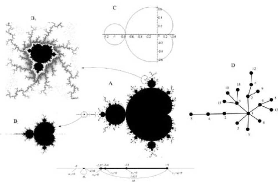
Figure 1: A. Mandelbrot set ${\cal M}_{2}$ for the family $f(x;c)=x^{2}+c$ [5]. The boundary of the black domain in the complex plane of $c$-variable consists of all values of $c$ where Julia set is reshuffled: as explained in [2] this happens when a stable orbit crosses an unstable one. A given orbit ${\cal O}$ is stable within and elementary domain, which is – with incredibly good accuracy – either a cardioid $c-c_{{\cal O}}=r_{{\cal O}}e^{i\phi}\left(1-\frac{1}{2}e^{i\phi}\right)$ at the center (root) of a cluster or a circle $c-c_{{\cal O}}=r_{{\cal O}}e^{i\phi}$ at the non-root nodes of the tree. Explanation of this fact (that only these two shapes occur and exactly in these roles: at roots and higher nodes respectively) is the task of the present paper. Projection to the line of real $c$ is also shown.     B. Two pieces of the Mandelbrot set ${\cal M}_{2}$ under microscope: exactly the same structures are seen as the central cluster in A, with the same central cardioids and attached circles. There are infinitely many such structures of different sizes $r_{{\cal O}}$ in ${\cal M}_{2}$, since $r_{{\cal O}}$ are very small, they are not actually seen in A, but can be easily studied with the help of the Fractal Explorer [4]. More numerical characteristics of the lowest elementary domains are collected in a Table in s.6.     C. Domains $(1)$ and $(2,1)$, obtained as numerical solutions of exact equations (2.3), see s.3.3.2. They coincide with domains, seen in A. This is non-trivial, because pictures A and B are obtained by absolutely different procedure (actually, black region consists of points $c$, with limited sequences $f^{\otimes n}(c)$), and there is no a priori reason for any parts of them to satisfy any kind of algebraic equations. Separation of Mandelbrot sets into domains, possessing an algebraic description, in particular the relation between pictures ${\bf A}$ and ${\bf C}$, is important property of iterated maps.     D. Tree structure of the central cluster (only a few lowest branches are shown), each branching occurs at the center of a new elementary domain, and the number at the vertex is the order of the periodic orbit, which is stable inside this domain. Thus elementary domains are naturally labeled by sequences of divisors, leading to the root of the tree. All other clusters are represented by exactly the same trees, only numbers are multiplied by the order of the root orbit. Thus entire ${\cal M}_{2}$ has a natural forest structure.

Figure 2: Mandelbrot set ${\cal M}_{3}$ for the family $f(x;c)=x^{3}+c$. Everything said about ${\cal M}_{2}$ is true in this case, only the place of simple cardioids at roots of clusters is taken by the two-cusp ones $c-c_{{\cal O}}\approx r_{{\cal O}}e^{i\phi}\left(1-\frac{1}{3}e^{2i\phi}\right)$. Descendant domains are nicely approximated by single-cusp cardioids $c-c_{{\cal O}}\approx r_{{\cal O}}e^{i\phi}\left(1-\frac{1}{2}e^{i\phi}\right)$, see eq.(10.7). No circles are present.

Figure 3: Mandelbrot set ${\cal M}_{4}$ for the family $f(x;c)=x^{4}+c$. Everything said about ${\cal M}_{2}$ is true in this case, only the place of simple cardioids at roots of clusters is taken by the three-cusp ones $c-c_{{\cal O}}\approx r_{{\cal O}}e^{i\phi}\left(1-\frac{1}{4}e^{3i\phi}\right)$. Descendant domains have the shape of deformed 2-cusp cardioid, $c-c_{{\cal O}}=r_{{\cal O}}e^{i\phi}\left(1-ae^{i\phi}+\frac{b}{3}e^{2i\phi}\right)$ with $a=2^{-4/3}\approx 0.40\ldots$ and $b\approx 11/(9\cdot 2^{2/3})=0.77\ldots$, see eq.(10.9). No circles or single-cusp cardioids are present.

Figure 4: Mandelbrot set ${\cal M}_{3-1}$ for the family $f(x;c)=ax^{3}+(1-a)x^{2}+c$ with two different values of additional parameter $a=4/5$ (A) and $a=2/3$ (B). Everything said about ${\cal M}_{2}$ is true in this case, only in addition to the simple single-cusp cardioids $c-c_{{\cal O}}=r_{{\cal O}}e^{i\phi}\left(1-\frac{1}{2}e^{i\phi}\right)$ in the role of central (root) domains there are also two-cusp ones, $c-c_{{\cal O}}=r_{{\cal O}}e^{i\phi}\left(1-\frac{1}{3}e^{2i\phi}\right)$. Moreover, for distinguished value $a=1$, see Fig.2, simple cardioids do not appear as central (root) domains of individual clusters at all – their place at roots is taken by 2-cusp curves. Instead for $a=1$ the single-cusp cardioids fully replace circles in the role of descendant domains. For smaller values of $a$ the simple cardioids start to emerge as roots (and circles – as descendants), but in remote clusters, at large distances from the central domain.    The central cluster in these pictures look a little asymmetric: this is wrong, and is an artefact of the erroneous algorithm, used to construct Mandelbrot sets by Fractal Explorer, see introductory remarks to s.4 below.

Mandelbrot sets are often considered as typical examples of ”fractal structures”, serving mostly for admiration, philosophical speculations and, perhaps, numerical exercises. However, as explained in [2], they can actually be subjected to systematic scientific investigation, in the style of experimental mathematics, with questions coming from direct observations and numerical experiments, and rigorous answers provided by knowledge of underlying algebro-geometric structures. Our presentation below can be considered as an example of this increasingly important approach to modern mathematical physics problems.

As explained in [2] – and clearly seen in Figs.1-4, – the Mandelbrot set consists of infinitely many separated clusters, of which only the central one is well seen in the main picture, while examples of smaller clusters are shown in auxiliary pictures with enhanced resolution. Though separated, clusters form a well organized structure: they are connected by ”trails”, populated with other clusters. Further, each cluster has its own tree structure, Fig.1.D, with two types of elementary domains: one type at the root of the tree and another type at all higher nodes (we call them descendants). Fig.4 demonstrates that a given Mandelbrot set can contain different types of clusters, while for special families $f(x;c)=x^{d}+c$, where maps possess additional $Z_{d-1}$ symmetry $x\rightarrow e^{2\pi in/(d-1)}x$, all clusters are of the same type. In Mandelbrot Set (i.e. for $d=2$) the root elementary domains are nearly ideal cardioids, Fig.5.A,

$$c-c_{{\cal O}}=r_{{\cal O}}e^{i\phi}\left(1-\frac{1}{2}\,e^{i\phi}\right)$$ (1.3)

while descendants are nearly ideal circles

$$c-c_{{\cal O}}=r_{{\cal O}}e^{i\phi}$$ (1.4)

For $d>2$ we have nearly ideal $(d-1)$-cusp cardioids, Fig.5,

$$c-c_{{\cal O}}=r_{{\cal O}}e^{i\phi}\left(1-\frac{1}{d}\,e^{i(d-1)\phi}\right)$$ (1.5)

at roots, while descendant domains are deformed cardioids with $d-2$ cusps and some non-vanishing coefficients $a_{k}$ in

$$c-c_{{\cal O}}=r_{{\cal O}}e^{i\phi}\left(1+\sum_{k=1}^{d-3}a_{k}e^{ik\phi}-\frac{1}{d-1}\,e^{i(d-2)\phi}\right)$$ (1.6)

Actual shapes of the domains slightly deviate from these ideal cardioids and circles and depend on particular cluster and node, but deviations are at the level of a few percents at most.

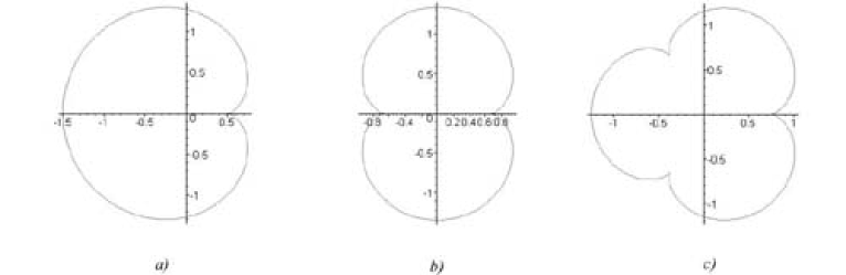
Figure 5: Cardioid curves described by the equations (1.3) and (5). These pictures reproduce the shapes of the central domains in Mandelbrot sets ${\cal M}_{d}$.   A. $d=2$. This is the central domain of ${\cal M}_{2}$ in Fig.1.   B. $d=3$. This is the central domain of ${\cal M}_{3}$ in Fig.2.   C. $d=4$. This is the central domain of ${\cal M}_{4}$ in Fig.3.

Each elementary domain is associated with some periodic orbit ${\cal O}$ of the map $f$, which is stable exactly within the domain. Thus the domain is labeled by the order $p$ of this orbit. This fact allows one to give an explicit analytical description of the domain’s shape, see eq.(2.3) below. However, there are many different periodic orbits with the same $p$ and thus many elementary domains with the same $p$. They differ by the choice of the root $c_{p}$ of the equation $f_{p}(c)\equiv f^{\circ p}(x=x_{cr};c)=x_{cr}$, which lies in the ”center” of the domain ($x_{cr}$ is the root of $f^{\prime}(x)$, $f^{\prime}(x_{cr},c)=0$, in most examples below $x_{cr}=0$). Some of these order-$p$ domains are at roots of some clusters, some at higher-level nodes, but in that case the root of the cluster should be associated with a divisor of $p$. Actually the tree underlying the cluster is the divisor tree, and the entire forest structure (i.e. collection of trees, associated with all clusters) is that of divisor forest of natural numbers. Accordingly, elementary domain is labeled by a sequence of integers $\Big{(}(p_{r}\cdot m_{1}\cdot\ldots\cdot m_{k})_{\alpha_{r,k}},\ \ldots,\ (p_{r}\cdot m_{1})_{\alpha_{r,1}},\ (p_{r})_{\alpha_{r}}\Big{)}$, to be read from rights to left. Sequence of multiples  $[m_{k},\ldots,m_{1}]\$ characterizes domain’s position in the tree, $k$ is the distance from the root, $p=(p_{r}\cdot m_{1}\cdot\ldots\cdot m_{k})$ is the period of the corresponding orbit, and $p_{r}$ is the order of the orbit, associated with the root domain. Since there can be many different root domains with the same $p_{r}$ in particular Mandelbrot set and many different descendants with the same $p$ in a given tree, there are additional labels $\alpha$, distinguishing between different trees in the forest with the same order $p_{r}$ at roots and between different branches with the same $p$ in each tree. While divisor trees are the same for all particular Mandelbrot sets, collections of ${\alpha}$’s are different: they are defined by the way the given section crosses the $p$-variety in the Universal Mandelbrot set, since it can be crossed many times, there are many traces of the same variety in the given section (in the role of either root or descendant domains) – and this is the origin of the forest and of the $\alpha$ parameters, which at the level of particular Mandelbrot set look somewhat arbitrary. At the level of UMS there is a single divisor tree and a section intersects it many times and cuts it into many similar trees: any cut-off branch looks like a separate tree and gives rise to a separate cluster. The memory of their common origin at UMS level is preserved in the trail structure, connecting the clusters, but its detailed description is not yet available.

Two adjacent elementary domains touch at exactly one point (i.e. along a complex-codimension-one variety in UMS), where their corresponding orbits cross and exchange stability. This important statement, however, needs to be treated carefully: as we shall see, in general (beyond the $x^{d}+c$ families) the elementary domains can overlap: there can be several stable orbits at the same value of $c$. This means that arbitrarily chosen $c$ is not a good coordinate on a Mandelbrot set, which is actually a fibration over a region in the complex-$c$ plane than a region per se. Fibration structure is inherited from Julia sheaf over the Mandelbrot set [2]. In this general situation the word touch is not fully informative: when different domains seem to overlap, they rather lie in different fibers over the same region on $c$-plane, and these fibers are sewed exactly at a single point, where the orbis cross. What we can show in simple $2d$ pictures are projections of the domains, these projections can overlap and touch at the orbit-crossing point. Touch means that the tangents to two domains are collinear, in practice this can be either a smooth touching (typical for crossing of orbits of different orders) or a cusp (when the orders are the same).

Crossing of orbits is possible only when the order of the smaller one (with domain lying closer to the root in the cluster) divides the order of the bigger one. Analytically, crossing takes place at the root of associated resultant. If the two orders differ by a factor of $2$, this is the celebrated period-doubling bifurcation [7, 8] – and the chain of exactly such bifurcations occurs along the real line in Fig.1,– but in fact doubling is in no way distinguished: bifurcation can multiply period by arbitrary integer $m$. Crossing of unstable orbits is not seen at the level of Mandelbrot sets shown in Figs.1-3,– to study these phenomena (also essential for bifurcations of Julia sets) the full (or Grand) Mandelbrot set should be considered. Actually, behind UMS there are even more fundamental entities: the Universal Julia Sheaf (UJS), consisting of all periodic orbits of all orders ”hanged” over the UMS, and the Grand UJS, including also all pre-orbits of periodic orbits. UMS is a projection of UJS, obtained by neglect of the phase-space dimension $x$, where the orbits live, and, as any projection, it can and does suffer from overlap ambiguities, namely, when two different stable orbits coexist at the same point of UMS.

We refer to [2] for further details and explanations. The task of this paper is to provide close-to-Earth illustrations of somewhat abstract formulations from the previous paragraphs and to fill some of the gaps left in [2], which concern three closely related subjects:

(i) the shape of elementary domains;

(ii) Feigenbaum indices, defining the ratio of sizes of adjacent elementary domains (immediate descendant as compared to its parent) from the ratio of the corresponding orders;

(iii) reshuffling of Mandelbrot set and its elementary sets under the change of selected family of functions, i.e. new properties of $2_{C}$-dimensional sections of Universal Mandelbrot set as compared to the $1_{C}$-dimensional sections.

In fact these subjects capture the main aspects of the general theory and at the same time they can be considered by simple methods of theoretical physics with minimal involvement of abstract algebro-geometric constructions. Even resultant and discriminant analysis, which was the main machinery in [2], will be at periphery of our simplified presentation in this paper.

As a key puzzle and a starting point for all considerations we choose the question, posed in the title of this paper: why exactly the cardioids (1.3) and circles (1.4) and exactly in the right places in the divisor forest emerge as the shapes of elementary domains of the Mandelbrot Set in Fig.1, and how this picture is continuously deformed into Figs.2 and 3.

As already shown in [2], cardioids (1.5) exactly describe the central domains $(1)$ for the families $x^{d}+c$, while in description of all other domains they straightforwardly appear in the ”small-size approximation” (SSA) to exact shape-defining eqs.(2.3). In what follows we

– explain, why for the $x^{d}+c\$ families the cardioids (1.5) do not exhaust all possible shapes: deformed cardioids (1.6) with one less cusp are also allowed;

– explain, why (1.5) appear exactly at roots of clusters, while all descendants have one cusp less: instead of this lacking cusp a descendant domain has a merging-point to the parent domain;

– provide a detailed description of interpolation between Mandelbrot sets and Julia sheafs for the families $x^{2}+c$ and $x^{3}+c$ (actually only the orbits of two lowest orders $p=1$ and $p=2$ will be analyzed, but this is already enough to reveal many interesting details of the process);

– demonstrate inaccuracy of Fractal Explorer [4] (and thus the underlying text-book interpretations of Mandelbrot sets) in application to UMS studies and appeal for the writing of corrected and fully adequate computer programs on the base of improved knowledge provided by [2];

– demonstrate high accuracy of the small-size approximation (SSA) in evaluation of various characteristics of the Mandelbrot Set by comparing its predictions for the (complex-valued) sizes $r_{{\cal O}}$ and Feigenbaum indices with exact answers (when they are already available) and experimental data provided by the Fractal Explorer [4].

Concerning the last story – about the SSA – it deserves saying that no theoretical explanation for its spectacular accuracy is known: particular corrections are not small, but various corrections always combine into a small quantity, whenever characteristics of Mandelbrot Set are evaluated. At the same time, as explained in [2], SSA fails completely in description of Julia sets; still it describes reasonably well the Mandelbrot sets for the families $x^{d}+c$ with $d>2$ (though some qualitative properties are spoiled, e.g. cusps are somewhat smoothed), but works much worse for interpolations between different $d$. In any case, today SSA remains the only available tool for theoretical investigation of high branches in divisor tree, in particular for approximate evaluation (rather than measuring) of various Feigenbaum indices – and for this purpose it works spectacularly well, even for $d>2$ and even for interpolations. Still rigorous algebro-geometric theory of Feigenbaum indices remains to be found.

We begin in s.2 from qualitative description of elementary domains supported by the limited amount of exactly-solvable examples in s.3: these include some non-trivial cases and, as usual, provide the solid ground for future approximate considerations. Section 4 is devoted to interpolation $\{ax^{3}+bx^{2}+c\}$ between the two best-known Mandelbrot sets: $\{x^{2}+c\}$ and $\{x^{3}+c\}$. Other examples of $3_{R}$-dimensional sections of UMS (actually of its central domain) are also given in this section. Then in s.5 we introduce the small-size approximation and present some calculations for the Mandelbrot Set. Their results are compared with experimental data in s.6. After some more borrowing SSA calculations in s.7, we discuss Feigenbaum indices in s.8. Section 10 is devoted to SSA consideration of some other Mandelbrot sets. Brief conclusions are collected in s.11.

2 The shape of elementary domains. Qualitative description

2.1 Defining equations

According to eqs.(10) and (38) of [2], the boundary of an elementary domain satisfies a pair of equations:

$$f\in{\cal M}\ \Leftrightarrow\ \left\{\begin{array}[]{c}F_{p}^{\prime}(x)+1=e^{i\theta}\\ F_{p}(x)=0\end{array}\right.$$ (2.3)

Here $F_{p}(x)=f^{\circ p}(x)-x$, prime denotes $x$-derivative and $\theta$ is a real-valued angle-parameter used to coordinatize the boundary of the domain (it can actually vary between $0$ and a multiple of $2\pi$, see below). After $x$ is excluded from the pair of equations (2.3), we obtain a real-codimension-one hypersurface in the space of functions $f$, i.e. a collection of curves $c(\theta)$ in $1_{C}$-dimensional Mandelbrot set. Particular curves – branches of $c(\theta)$ – are boundaries of particular elementary domains of the order $p$, root and descendant.

2.2 Cusps

Even if function $c(\theta)$ is smooth, the corresponding curve in the complex-$c$ plane can be singular. Generical singularity is self-intersection, which takes place when $c(\theta_{1})=c(\theta_{2})$ for $\theta_{1}\neq\theta_{2}$. Of interest for us are cusps: degenerated self-intersections, appearing in the limit when $\theta_{2}\rightarrow\theta_{1}$, i.e. when $\frac{dc}{d\theta}(\theta_{0})=0$ at some $\theta_{0}$. In the vicinity of such point $\sigma(\vartheta)=c(\theta)-c(\theta_{0})=a\vartheta^{2}+b\vartheta^{3}+\ldots$, where $\vartheta=\theta-\theta_{0}$. This means that

$${\rm Re}\left(\frac{\sigma}{a}\right)=\vartheta^{2}+\ldots,\ \ \ \ {\rm while}\ \ \ \ {\rm Im}\left(\frac{\sigma}{a}\right)={\rm Im}\left(\frac{b}{a}\right)\vartheta^{3}+\ldots$$ (2.4)

i.e.

$${\rm Im}\left(\frac{\sigma}{a}\right)\sim{\rm Im}\left(\frac{b}{a}\right)\left\{{\rm Re}\left(\frac{\sigma}{a}\right)\right\}^{3/2}$$ (2.5)

Thus we see that a cusp emerges at points where $dc/d\theta=0$ and its orientation in the complex-$c$ plane is defined by the phase of the complex-valued parameter $a$.

If $\ {\rm Im}(b/a)=0$, i.e.

$${\rm Im}\left(\frac{d^{3}c/d\theta^{3}}{dc/d\theta}\right)=0$$ (2.6)

along with $dc/d\theta=0$, then a self-intersection point collides with the cusp and disappears.

2.3 Cardioids

Cardioids are represented by polynomials of the unimodular variable, they form the simplest natural class of curves with cusps.

For quadratic cardioid,

$$c=r\left(e^{i\phi}+ae^{2i\phi}\right)\ =\ \frac{r}{4a}\Big{(}(1+2ae^{i\phi})^{2}-1\Big{)},$$ (2.7)

derivative vanishes, $dc/d\phi=0$, when $2ae^{i\phi}=-1$. This never happens if $|a|\neq\frac{1}{2}$. Thus a cusp (and exactly one) occurs only when $|a|=\frac{1}{2}$, the curve is everywhere smooth for $|a|<\frac{1}{2}$ and possesses one self-intersection for $|a|>\frac{1}{2}$.

For cubic cardioid,

$$c=r\left(e^{i\phi}+ae^{2i\phi}+be^{3i\phi}\right),$$ (2.8)

derivative $dc/d\phi=0$ vanishes when

$$1+2ae^{i\phi}+3be^{2i\phi}=0,$$ (2.9)

i.e. when the r.h.s. $e^{-i\phi}=-a\pm\sqrt{a^{2}-3b}\$ has unit modulus. If $a$ and $b$ are real, then cusp can occur when either $1+2a+3b=0$ (then there is one cusp at $\phi=0$, unless $a=0$ and $b=-\frac{1}{3}$, when another cusp appears at $\phi=\pi$, see Fig.6) or $-1<a<1,\ b=+1/3$ (then two cusps arise at $\phi=\pm\phi_{0}\neq 0,\pi$). In general, (2.9) defines a hypersurface of real codimension one in the space of complex parameters $a$ and $b$ (parameterized by $\phi$), where cubic cardioids (2.8) have cusps (one or two).

Transition point (2.6) between a phase with and without self-intersection is defined by a system of two equations,

$$\left\{\begin{array}[]{c}{dc}/{d\phi}\sim 1+2a+3b=0\\ {d^{3}c}/{d\phi^{3}}\sim 1+8a+27b=0\end{array}\right.$$

i.e. $a=-4/5$ and $b=1/5$, see Fig.6.

MAPLE program for cardioid studies, which was used to generate Figs.5 and 6, can be found in Appendix to this paper, see s.12.1.

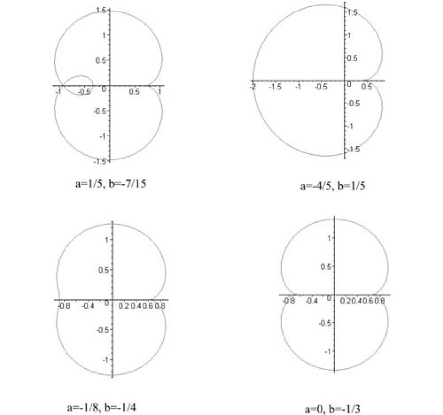
Figure 6: Cardioids with cusps and self-intersections. The cusp-possessing subset in the family (2.8) with $1+2a+3b=0$ is shown.  A. $a=\frac{1}{5}$, $b=-\frac{7}{15}$. Both cusp and self-intersection are present.  B. $a=-\frac{4}{5}$, $b=\frac{1}{5}$. This is the point where self-intersection point hits the cusp and disappears.  C. $a=-\frac{1}{8}$, $b=-\frac{1}{4}$. A single cusp is present at $\phi=0$.   D. $a=0$, $b=-\frac{1}{3}$. The second cusp appears at $\phi=\pi$.

2.4 Cusps in the boundaries of elementary domains

The second component of eq.(2.3) implies that

$$\dot{F}_{p}\frac{dc}{d\theta}=-F^{\prime}_{p}\frac{dx}{d\theta}$$ (2.10)

(dot and prime denote $c$- and $x$-derivatives respectively), so that $\frac{dc}{d\theta}=0$ when $F^{\prime}_{p}=0$, provided $\dot{F}_{p}\neq 0$ at the same point. Together with the first eq.(2.3) this means that cusp can occur only when $\theta=0$. Thus the number of cusps depends essentially on the range of variation of $\theta$-variable. If $\theta$ runs from $0$ to $2\pi(d-1)$, we can expect up to $d-1$ cusps to occur.

2.5 Why descendant domains have one cusp less than the root ones?

Descendant domain differs from the root one, because it always has one special point at the boundary where $F^{\prime}=0$ and $\dot{F}=0$ together. This means that there is no cusp at this point, and if the total number of zeroes of $F^{\prime}$ at the boundary was $d-1$, but the domain was a descendant, then the total number of cusps will be $d-2$.

Characteristic feature of any descendant is reducibility of the corresponding function $F_{mp}$: it is divisible by $F_{p}$ of a parent domain,

$$F_{mp}(x)=\tilde{G}_{mp}(x)F_{p}(x),$$ (2.11)

(in variance with $G_{mp}$ from ref.[2] such $\tilde{G}_{mp}$ can still be reducible, but this does not matter for our purposes in this paper). Then $F^{\prime}_{mp}=\tilde{G}_{mp}^{\prime}F_{p}+\tilde{G}_{mp}F_{p}^{\prime}$ and $\dot{F}_{mp}=\dot{\tilde{G}}_{mp}F_{p}+\tilde{G}_{mp}\dot{F}_{p}$ vanish simultaneously whenever both $F_{p}=0$ and $\tilde{G}_{mp}=0$, i.e. when $x$ belongs simultaneously to orbits of orders $p$ and $mp$. According to [2] the last two equations possess exactly one common zero at the boundary of descendant domain: it is exactly the merging point, where descendant domain is attached to the parent one, and in the $c$-space it is a zero of the resultant $R(\tilde{G}_{mp},F_{p})$.

Discriminant $D(\tilde{G}_{mp})$ also vanishes when $R(\tilde{G}_{mp},F_{p})=0$, because different points of the order-$mp$ orbit (roots of $G_{mp}$) should merge $m$-wise to merge with the points of the order $p$-orbit (roots of $F_{p}$). Of more interest are other zeroes of $D(G_{mp})$, representing crossings of different orbits of order $mp$.

3 Exact results about elementary domains

This section is devoted to exactly-solvable examples. Here exact solvability means not obligatory explicit analytical solutions – though they will also be considered. Whenever the problem can be effectively studied by user-friendly computer tools like MAPLE or Mathematica, it is considered equally (and may be even better) solvable as if explicit formulas were derived. We shall see that sometime the best way to analyze such explicit formula is to generate its plot with the help of the same MAPLE. One should keep in mind, however, that the number of problems solvable in this way is also very limited: in most cases even clearly formulated algebraic problems can be handled only by specially designed programs, which usually could but never were written. This makes such problems potentially solvable (as many other hot problems in theoretical physics), but they are clearly different from practically solvable. We also distinguish these solvable problems from those which are effectively solved, but only approximately: under certain additional assumptions or when improving of accuracy is increasingly difficult (like it happens, for example, in perturbation theory). We turn to approximate methods in ss.5-10. Before we are going to describe what is known today at exact level.

Our primary goal is to understand what is the domain of variation of the $\theta$-variable – because we already know from s.2.4 that it is its size that defines the number of cusps, both for root and descendant domains. Moreover, we want to see how this variation domain is changed in transition from one Mandelbrot set to another, i.e. to study the bifurcations of Mandelbrot sets themselves, which happen in complex-codimension-two in the Universal Mandelbrot space. Examples will be also used in other sections, where we derive (approximately) the analytical shape of the domains.

3.1 Elementary domains of order $p=1$ for special Mandelbrot sets

Let us consider a Mandelbrot set for a one-parametric family

$$f(x,c)=P_{d}(x)+c$$ (3.1)

with polynomial $P_{d}(x)$ of degree $d$ (we do not require it to be homogeneous $x^{d}$ at this moment). Additive dependence on $c$-parameter considerably simplifies consideration of such families.

For $p=1$ equations (2.3) state simply that

$$\left\{\begin{array}[]{c}P^{\prime}_{d}(x)=e^{i\theta}\\ c=x-P_{d}(x)\end{array}\right.$$ (3.4)

and for every particular choice of $P_{d}(x)$ the function $c(\theta)$ can be easily plotted with the help of MAPLE or Mathematica. Moreover, there are two important examples when even analytical solution is immediately available.

The first case is homogeneous $P_{d}(x)=x^{d}$, associated with the standard $Z_{d-1}$-symmetric Mandelbrot sets ${\cal M}_{d}$. The second case is generic cubic polynomial $P_{3}(x)=x^{3}+ax^{2}+bx$: associated family of Mandelbrot sets ${\cal M}_{3}(a,b)$ interpolates between ${\cal M}_{2}={\cal M}_{3}(\infty,0)$ and ${\cal M}_{3}={\cal M}_{3}(0,0)$. For such interpolation one can also use a one-dimensional and ”better” parameterized family ${\cal M}_{2,3}(a)$ with $P_{3}(x)=ax^{3}+(1-a)x^{2}$ (then ${\cal M}_{2}={\cal M}_{2,3}(0)$ and ${\cal M}_{3}={\cal M}_{2,3}(1)$).

3.2 Analytically solvable examples for $p=1$

3.2.1 Homogeneous $P_{d}(x)$

For homogeneous $P_{d}(x)=x^{d}$ eq.(3.4) converts directly into (1.5):

$$\left\{\begin{array}[]{c}dx^{d-1}=e^{i(d-1)\phi},\ \ \ \ \ \ {\rm i.e.}\ \ \ \ \ \ x=r(d)e^{i\phi}\\ \\ c=x\Big{(}1-x^{d-1}\Big{)}=r(d)e^{i\phi}\Big{(}1-\frac{1}{d}\,e^{i(d-1)\phi}\Big{)}\end{array}\right.$$ (3.8)

where $r(d)=d^{-\frac{1}{d-1}}$ and $\phi=\frac{\theta}{d-1}$. It is obvious that in this case $\theta$ changes from $0$ to $2\pi(d-1)$ and $\phi$ is the right angle-parameter.

Now we can use another solvable example with $P_{3}(x)$ in order to deform these ideal cardioids and see how their order (number of cusps) can actually change in interpolation between $x^{2}$ and $x^{3}$, see s.4.

3.2.2 Cubic polynomial

For $P_{3}(x)=ax^{3}+bx^{2}$ the first equation in (3.4), $\ 3ax^{2}+2bx=e^{i\theta}$, is quadratic in $x$ and has explicit analytic solution:

$$x=\frac{-b\pm\sqrt{b^{2}+3ae^{i\theta}}}{3a}$$ (3.9)

(only the ”+” branch has a finite limit at $a\ \rightarrow 0$). Substituting this into the second equation (3.4), $\ c_{1}=x-P_{3}(x)=-ax^{3}-bx^{2}+x$, we obtain the analytical expression for the boundary of the root domain of the central cluster for arbitrary values of complex parameters $a\$ and $b$:

$$c_{1}=\frac{\left(b\mp\sqrt{b^{2}+3ae^{i\theta}}\right)\left(5b^{3}-9a+3ae^{i\theta}\mp 5b\sqrt{b^{2}+3ae^{i\theta}}\right)}{27a^{2}}$$ (3.10)

Clearly, the phase transition line, separating the two regimes – $\theta=2\phi$ (near $b=0$) and $\theta=\phi$ (near $a\ =0$), – is $|b|^{2}=3|a\ |$. If $b=1-a\$, see s.4, it crosses the real-$a\$ line at $a_{cr}^{\pm}=\frac{5\pm\sqrt{21}}{2}$, i.e. $a^{-}_{cr}=0.208712\ldots$ and $a^{+}_{cr}=5-a^{-}_{cr}=4.791288\ldots$

3.3 Solvable examples for $p=2$

3.3.1 Equations in case of separated $c$-dependence

For $p=2$ equations (2.3) can be rewritten as follows:

$$\left\{\begin{array}[]{c}f(x)=z;\\ f(z)=x;\\ f^{\prime}(z)f^{\prime}(x)=e^{i\theta}\end{array}\right.$$ (3.14)

and when

$$f(x,c)=P(x)+c$$ (3.15)

with $c$-independent $P(x)$, as

$$\left\{\begin{array}[]{c}P(z)+z=P(x)+x;\\ P^{\prime}(z)P^{\prime}(x)=e^{i\theta}\end{array}\right.$$ (3.18)

Then $c(\theta)$ can be defined from

$$c=z-P(x)=x-P(z).$$ (3.19)

Since we did not factor out $F_{1}$ from $F_{2}=G_{2}F_{1}$, these equations describe not only the $(2)$ and $(2,1)$ domains, but also the $(1)$ ones. The $(1)$ domains satisfy the system (3.18) with first equation substituted by $x=z$, while for the $(2)$ and $(2,1)$ domains it should be substituted by $\frac{P(z)-P(x)}{z-x}=-1$.

3.3.2 MAPLE-generated solution for homogeneous $P_{d}(x)$

For $P_{d}(x)=x^{d}$ the second equation in (3.18) can be solved explicitly:

$$xz=d^{-\frac{2}{d-1}}e^{i\varphi}\equiv\xi$$ (3.20)

where we substituted $\theta=(d-1)\phi$. Then the first equation (3.18) turns into

$$x^{d}-\frac{\xi^{d}}{x^{d}}=-x+\frac{\xi}{x}$$ (3.21)

One solution, $x=\xi/x$, i.e. simply $x=z=d^{-\frac{1}{d-1}}e^{i\phi}$ with $\phi=\frac{\varphi}{2}$ changing from $0$ to $2\pi$, provides

$$c_{1}(\phi)=z-x^{d}=x-z^{d}=d^{-\frac{1}{d-1}}e^{i\phi}\left(1-\frac{1}{d}\,e^{i\phi}\right)$$ (3.22)

which is our familiar eq.(3.8) for the central root domain $(1)$, with examples shown in Fig.5.

Remaining solutions, describing the root $(2)$ and descendant $(2,1)$ domains, can be solved by MAPLE or Mathematica, see Fig.7. In these solutions $\varphi=\phi$. No root $(2)$ domains occur for homogeneous $P_{d}(x)=x^{d}$, but this is a peculiarity of both homogeneity and $p=2$: root domains $(p)$ exist for all $p\neq 2$ even if $P_{d}(x)=x^{d}$, and $(2)$ domains are normally present for generic non-homogeneous $P_{d}(x)$, see s.4 for examples.

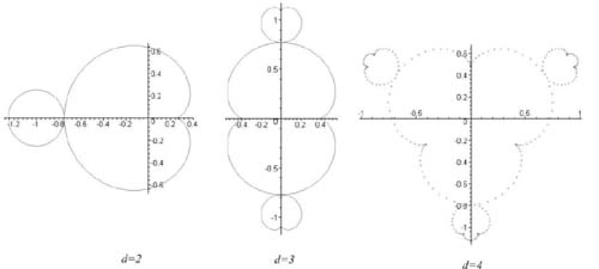
Figure 7: The first two domains $(1)$ and $(2,1)$ of the central cluster, obtained from solving eq.(3.21) with the help of MAPLE. In the case of $d=2$ and $3$ analytical solutions are also available: see eqs.(3.26) and (3.28) respectively (and they are explicitly used by MAPLE). A: $d=2$, $f(x,c)=x^{2}+c$, B: $d=3$, $f(x,c)=x^{3}+c$, C: $d=3$, $f(x,c)=x^{4}+c$, D: $d=4$, $f(x,c)=x^{4}+c$. Mandelbrot set for $f(x,c)=x^{d}+c$ has $Z^{d-1}$ symmetry under rotations around the point $c=0$.

3.3.3 Analytical solutions for homogeneous $P_{2}(x)$ and $P_{3}(x)$

For $d=2$ and $d=3$ analytical solutions are also available. Indeed, then eqs.(3.21), after exclusion of solutions $x=z$, turn into

$${\bf d=2:}\ \ \ \ \ x+z+1=x+\frac{\xi}{x}+1=0,\ \ \ \ \xi=\frac{1}{4}e^{i\phi}$$ (3.23)

and

$${\bf d=3:}\ \ \ \ \ x^{2}+xz+z^{2}=x^{2}+\xi+\frac{\xi^{2}}{x^{2}}=-1,\ \ \ \ \xi=\frac{1}{3}e^{i\phi}$$ (3.24)

respectively, which are explicitly solvable quadratic and biquadratic equations.

Then it follows that for $d=2$

$$x=-\frac{1}{2}\pm\frac{1}{2}\sqrt{1-e^{i\phi}},$$

$$z=-\frac{1}{2}\mp\frac{1}{2}\sqrt{1-e^{i\phi}}$$ (3.25)

and

$$c_{2,1}(\phi)=z-x^{2}=x-z^{2}=-1+\frac{1}{4}e^{i\phi}$$ (3.26)

is an ideal circle of radius $r_{2,1}=\frac{1}{4}$ centered at $c_{2,1}=-1$, see Fig.7.A.

Similarly for $d=3$

$$x=\pm\frac{1}{\sqrt{2}}\sqrt{-1-\frac{1}{3}e^{i\phi}\pm\sqrt{1+\frac{2}{3}e^{i\phi}-\frac{1}{3}e^{2i\phi}}},$$

$$z=\pm\frac{1}{\sqrt{2}}\sqrt{-1-\frac{1}{3}e^{i\phi}\pm\sqrt{1+\frac{2}{3}e^{i\phi}-\frac{1}{3}e^{2i\phi}}}$$ (3.27)

and, see Fig.7.B,

$$c_{2,1}(\phi)=z-x^{3}=x-z^{3}$$ (3.28)

In both examples $\phi=\varphi$ changes in between $0$ and $2\pi$.

3.3.4 MAPLE-generated solution for arbitrary cubic polynomial

For arbitrary cubic $P_{3}(x)$ the second equation in (3.18) is quadratic in $z$ and can be solved explicitly. After substitution of this $z(x)$ the first equation can be solved with the help of MAPLE or Mathematica and (3.19) produces the final answer. This is how Figs.8–29 are obtained.

4 The first two elementary domains in interpolation between ${\cal M}_{2}$ and ${\cal M}_{3}$

After equations are solved, we can turn to description of solutions.

For particular homogeneous polynomials $P_{d}(x)=x^{d}$ we obtained the well known shapes of central domains in ${\cal M}_{d}$ Mandelbrot sets, see Fig.7, – only this time this is not a result of computer simulations by Fractal Explorer, the shapes are now obtained as solutions (sometime even analytical) to algebraic equations (2.3).

Even more interesting is the possibility to study quantitatively interpolation between the ${\cal M}_{2}$ and ${\cal M}_{3}$ sets. So far only qualitative description was known [2], and the usual computer simulations fail. Such simulations [5] are often based on the study of the sequence $f^{\circ n}(c)$, i.e. the orbit of $x_{cr}=0$. Interior of the Mandelbrot space, i.e. the black regions in Figs.1–4, is assumed to consist of all functions $f$ where this sequence is bounded and does not go away to infinity. However, this assumption is not always true and then this simple algorithm fails – and Fig.4 is the first example. The reasons for failure can be different: from $x_{cr}\neq 0$ to attraction of unstable orbits to finite, rather than to infinitely remote ones. There is a strong need to cure this problem and make a modification of Fractal Explorer which would treat properly any kind of Mandelbrot set.

4.1 Particular Mandelbrot sets ${\cal M}_{2,3}(a)$ for the families $ax^{3}+(1-a)x^{2}+c$ at different values of $a$

At $a=0$ the Mandelbrot Set acquires its standard form, Fig.1, and its first two domains, $(1)$ and attached $(2,1)$, are shown in Figs.1.C and 7.A.

4.1.1 Vicinity of the Mandelbrot Set: small $|a|$

However, as soon as $a$ infinitesimally deviates from $a=0$, it gets clear that Fig.1 has a twin: an exact copy of the same shape and size, but with opposite orientation – a mirror twin, – located at infinity of the complex-$c$ plane. As $|a|$ grows, the twin moves closer, and Figs.8 and 9 show its location at $a=\pm 1/10$ (the sizes of the domains are practically the same as in Fig.1 – just the scale of the picture is different, because the twin of Fig.1 is still far away). Moreover, it appears that additional mirror pair of $(2)_{\pm}$ domains – roots of two more clusters – were hidden at infinity of $c$ plane and are now located in between the two root domains $(1)_{\pm}$ for positive $a>0$ and on the opposite sides of those for negative $a<0$. Since for small $a$ these domains are tiny as compared to the $(1)$ and $(2,1)$, they can be easily overlooked, therefore one of them is marked by a circle and shown in a bigger scale in a separate picture at the right low corner. Clearly this root $(2)_{-}$ domain has cardioid shape and is exact copy of the root domain $(1)_{-}$, only smaller. In fact it has a $(4,2)_{-}$ domain attached to it in exactly the same manner as $(2,1)_{-}$ is attached to $(1)_{-}$ – it is not shown, because we explicitly construct only domains of orders $p=1$ and $2$. For interested reader we add also slices of the Julia sheaf: show behavior of the orbits in the $x$ space with the change of $c$, which becomes more and more interesting as we go far from the ”pure” points $a=0$ and $a=1$. The problem is that Julia sheaf is embedded into a $4_{R}d=2_{C}d$ space, with complex $x$ and $c$, and can not be shown in full, even if $a$ is fixed. Therefore different sections and projections are presented, $2_{R}$- and $3_{R}$-dimensional. $3_{R}$-dimensional are especially informative, but only when presented on computer screen, where they can be rotated and regarded from different angles. This advantage is lost in the printed version of the text, but one can either use simple MAPLE programs, collected in s.12 below or directly look at the results in [6].

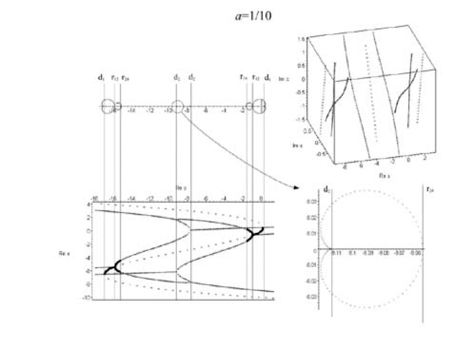
Figure 8: The picture in the left upper corner represents the Mandelbrot set for the family $ax^{3}+(1-a)x^{2}+c$ with $a=1/10$. This is the picture in complex $c$ plane and shown are only domains, associated with the order $p=1$ and $p=2$ orbits. The orbits themselves lie in the complex $x$ plane and form the Julia sheaf over Mandelbrot set. Julia sheaf itself is a $1_{C}d$ complex variety, embedded into a $2_{C}d$ complex space and can not be shown in an ordinary drawing. Instead two different views, one $2_{R}$-dimensional, another $3_{R}$-dimensional (at fixed ${\rm Re}(c)=C(a)$) are shown in the low left and upper right corners respectively. As all other three dimensional sections in this paper, it can be rotated and looked from different angles: this clarifies the pattern a lot, but can be done only on computer screen, see ref.[6]. (In particular, there are NO intersecting orbits in this section – the seeming intersection is an artefact of the drawing, resolved by rotation of the picture). Dilute lines represent the three order-$1$ orbits, while dense lines – the six order-$2$ orbits. In $2_{R}d$ picture solid segments show stable orbits: those of order $1$ are stable inside the $(1)_{\pm}$ domains of the Mandelbrot set, those of order $2$ – inside the $(2,1)_{\pm}$ and $(2)_{\pm}$ domains (the last two are two small to have the corresponding solid segments seen in our pictures). Enlarged picture of the $(2)_{-}$ domain – a root of a new cluster – is shown in the low right corner, and it is clear that it is an exact diminished copy of the root $(1)_{-}$ domain. $(2)_{+}$ is its exact mirror copy, in accordance with $Z_{2}$ symmetry of the Mandelbrot set w.r.t. the vertical line ${\rm Re}(c)=C(0.1)=-8.4$. Shown are also the roots $c=d_{1,2}$ of discriminants $D_{1}$ and $D_{2}$ and $c=r_{12}$, $c=r_{24}$ of the resultants $R_{12}$ and $R_{24}$ (they lye at intersections of vertical lines with the real-$c$ axis). According to [2], the last two are the crossing points of the orbits of orders $1$ and $2$ and $2$ and $4$, define merging points between the domains $(2,1)$ and $(1)$ and between $(4,2)$ and $(2,1)$ respectively, and thus define the stability segments of orbits of orders $1$ and $2$. Similarly, discriminant zeroes are intersection points of the orbits of the same order: $p=1$ with $p=1$ and $p=2$ with $p=2$. $2_{R}d$ view in the low left corner is in fact a section of the $c$ plane with given ${\rm Im}(c)=0$ and projection on the ${\rm Re}(x)$ plane. Accordingly, when two real-valued orbits intersect and become complex-valued, they remain shown in the picture, but since they are complex conjugate, two lines are projected onto one – this should be taken into account in analysis of the figure.

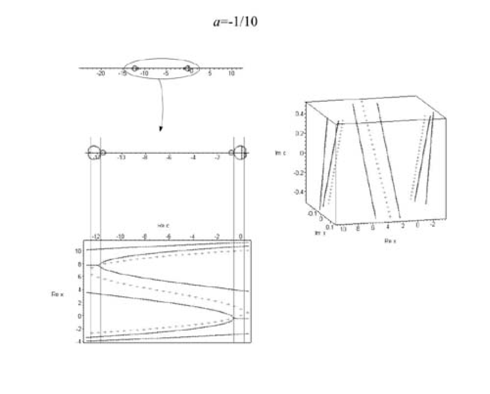
Figure 9: Analogous picture for negative real $a=-1/10$. The only essential difference from Fig.8 is that the two root domains $(2)_{\pm}$ are not in between the two $(1)_{\pm}$, but on the opposite sides of those. In other words, at $a=0$ the $(2)$ domains pass through $(1)_{-}$, so that $(2)_{+}$ re-appears from $c=+\infty$, while $(2)_{-}$ returns back from $c=-\infty$, but slower than $(1)_{-}$, see also Fig.10. Because of this, when $|a|$ increases further in the direction of negative $a$, the overlap will occur between the domains $(2,1)_{-}$ and $(2,1)_{+}$, unlike in the positive-$a$ case, where $(2)_{-}$ and $(2)_{+}$ will be the first to meet.

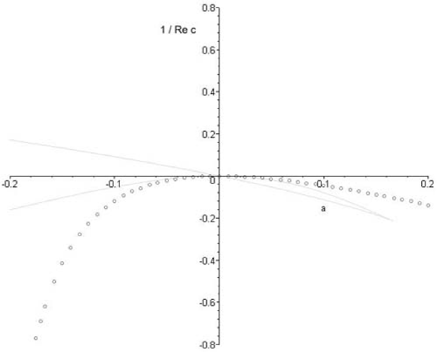
Figure 10: Behavior in the vicinity of $a=0$ of the root domains $(1)_{-}$ and $(2)_{\pm}$, denoted respectively by circles and solid lines???. As $a\rightarrow 0$, these three domains, together with their entire clusters, travel to infinity in the complex-$c$ plane, therefore the picture is drawn in coordinate $1/c$ (only real values of $c$ are plotted). The Mandelbrot Set from Fig.1, including the central root domain $(1)_{+}$, stays in the vicinity of $c=0$ and is not shown in this picture. Behavior of the $(2)_{+}$ and $(2)_{-}$ domains is somewhat different: the former one re-appears from infinity at the opposite end of the ${\rm Re}(c)$ axis, while the latter one returns from the same end, only exchanges positions with the $(1)_{-}$ domain – in full accordance with Figs.8 and 9. All the domains and in fact the entire clusters shrink to a single point at $a=0$, the reason for this is the choice of a very singular map in homogeneous coordinates: $\big{(}x,\ y\big{)}\longrightarrow\big{(}ax^{3}+bx^{2}y+cy^{3},\ y^{3}\big{)}$. Such singular behavior at $a=0$ would be smoothed and become similar to bifurcations at finite $a$, shown in forthcoming pictures, if $y^{3}$ is substituted by generic cubic polynomial. See [3] for related considerations.

All Mandelbrot sets ${\cal M}_{2,3}(a)$ possess a discrete $Z_{2}$ symmetry under reflection w.r.t. the vertical line

$${\rm Re}(c)=C(a)=-\frac{b}{3a}\left(1+\frac{2b^{2}}{9a}\right)$$ (4.1)

with $b=1-a$, which is lifted to entire Julia sheaf over ${\cal M}_{2,3}(a)$:

$$\begin{array}[]{ccc}\tilde{x}=x+\frac{b}{3a}&\ \longrightarrow&-\tilde{x}\\ \tilde{c}=c-C(a)&\ \longrightarrow&-\tilde{c}\end{array}$$ (4.4)

For example, the equation $F_{1}(x,c)=0$ for the first-order periodic orbits is obviously symmetric, since $F_{1}(x,c)=ax^{3}+bx^{2}+c-x=a\tilde{x}^{3}-\left(1+\frac{b^{2}}{3a}\right)\tilde{x}+\tilde{c}$. In accordance with this symmetry, the $(1)_{-}$ domain – the twin of the $(1)_{+}$ domain, centered at $c=0$,– is the mirror-reflected cardioid with center at $c=2C(a)$. Similarly, the two next root domains $(2)_{\pm}$ are centered at $c_{2+}=-\frac{1}{a}+2+O(a)$ and $c_{2-}=2C(a)-c_{2+}$, see s.6.4.5 of ref.[2]. Since $c_{2+}$ is odd function of $a$ for small $a$, while $c_{1-}$ is even, it is clear that they exchange order when $a$ goes through zero – in accordance with what is shown in Figs.8, 9 and 10.

4.1.2 Overlapping domains

As $|a|$ increases, the two domains $(1)_{\pm}$ move closer. The speed of approaching is somewhat different for positive and negative $a$. At some stage of this movement two different clusters unavoidably meet. There are, however, two sorts of meeting: overlap and collision. For above-explained reasons it is still difficult to analyze the behavior of entire clusters. Approximate results about clusters (or, better, possible approach to their future derivation) will be discussed in the last sections 5-10 of this paper. Exact results to be considered right now concern meetings of the low ($1$ and $2$) order domains. Overlap of these domains takes place soon after it happens to the upper $(p=\infty)$ leaves of the clusters, while collision can start at the $p=\infty$ leaves, but can also begin at the low-$p$ level.

Overlaps and collisions of particular domains occur when zeroes of the corresponding resultants collide, i.e. are controlled by zeroes of double-resultants, like $c$-discriminants of the $x$-resultants, listed in the following table (italic lines are quotations from MAPLE program, boldfaced are real-valued roots, belonging to the segment $0\leq a\leq 1$).

Two zeroes of $D1$ merge at $a=-\frac{1\pm i\sqrt{3}}{2}$.

$discrim(discrim(F1,x),c)=96*a^{2}+112*a^{3}+96*a^{4}+48*a+48*a^{5}+16+16*a^{6}$

Two zeroes of $R_{12}$ merge at $a=\frac{5\pm\sqrt{21}}{2}$ and at $a=-2\pm\sqrt{3}$.

Only one of these points, $a=\frac{5-\sqrt{21}}{2}=0.20871215\ldots$ belongs to the interval $0<a<1$ on a real-$a$ line.

$discrim(resultant(G2,F1,x),c)=16*a^{10}*(a^{2}+4*a+1)^{2}*(a^{2}-5*a+1)$

Two zeroes of $D2$ merge at $a=4\pm\sqrt{15}$.

$discrim\Big{(}\sqrt{discrim(G2,x)/R_{12}}\Big{)}\sim(a^{2}-8*a+1)^{3}$

Two zeroes of $R_{24}$ merge at

$a=0.1487496031\pm 0.03597329725i$, $a=6.351250397\pm 1.535973297i$,

$a=-4.485250968,-0.2229529645,\ {\bf 0.1163898556},\ 8.591814077=1/0.1163898556$,

$a={\bf 0.1497297977},\ 6.678697327=1/0.1497297977$,

$a=0.5857864376\pm 0.8104654524i$,

$a=\frac{9\pm\sqrt{65}}{4}$.

The four series correspond to zeroes of the four factors in

$discrim\Big{(}\sqrt{resultant(G2,G4,x)},c\Big{)}\sim(2*a^{4}-26*a^{3}+93*a^{2}-26*a+2)\cdot$

$\cdot(a^{4}-4*a^{3}-39*a^{2}-4*a+1)^{2}(a^{4}-8*a^{3}+10*a^{2}-8*a+1)^{2}(2*a^{2}-9*a+2)^{4}$

Derivative $\partial d_{1}^{-}/\partial a$ for the zero $d_{1}^{-}$ of discriminant $D_{1}$, which defines the position of the cusp in the $(1)_{-}$ domain, defines the speed of motion of the cluster $(1)_{-}$ with the change of $a$. Since for small $a$ all the clusters are diminished copies of the central one in Fig.1, with all the same proportions one can actually predict what happens to clusters from the data about their root domains.

The first event to happen on our way from $a=0$ is overlap. If $a>0$ this is the overlap of domains $(2)_{+}$ and $(2)_{-}$, while if $a<0$ it is that of $(2,1)_{+}$ and $(2,1)_{-}$. The two domains of order $2$ overlap when the two zeroes of $R_{24}$ coincide. If we move from $a=0$ along the real-$a$ line this first happens at $a=0.1163898556\ldots$ if $a>0$ and at $a=-0.2229529645\ldots$ if $a<0$. Figs.11, and 12 show Mandelbrot sets soon after these points are passed.

It is clear from these pictures, that when overlap occurs, nothing interesting happens to the orbits – and this is what makes overlap different form collision, when intersection of orbits takes place, see below. Overlap means simply that two (or more) different orbits are simultaneously stable at the same value of $c$: in this case these are two order-$2$ orbits. When overlap increases, it involves the $(1)_{\pm}$ domains and at the same values of $c$ can coexist two stable orbits of other orders: $2$ and $1$ (Fig.13) and $1$ and $1$ (Fig.14). For $a<-1$ the further increase of $|a|$ leads to diminishing of the overlap: the story repeats in the opposite order, the overlap picture for $a=-4$ ressembles that for $a=-0.25$ (shown in Fig.13), for $a=-4.(4)$ – that for $a=-0.225$ (shown in Fig.12), and after that the overlap disappears.

The reason for reversed evolution is that the family ${\cal M}_{2,3}(a)$ and even its Julia sheaf has a discrete ”symmetry” w.r.t. inversion of parameter $a\rightarrow 1/a$:

$$x(a^{-1},\theta)=-ax(a,\theta),$$

$$c(a^{-1},\theta)=-ac(a,\theta)$$ (4.5)

This symmetry complements the (4.4) of particular Mandelbrot sets at fixed $a$, and it allows to consider only the variation of $a$ within interval $|a|\leq 1$, all Mandelbrot sets outside this interval are exact rescaled copies of those inside.

More interesting things are taking place for positive $a$.

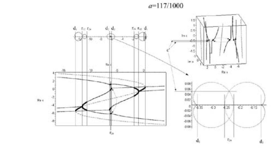
Figure 11: Domains of the orders $p=1,2$ of the Mandelbrot set ${\cal M}_{2,3}(a)$ (domains of orders $p=1,2$) at $a=0.117$, immediately after the two root domains $(2)_{\pm}$ touched at $a=0.1163898556\ldots$. Now they overlap: for $c$ in close vicinity of $c=-6.24$ there are two stable order-$2$ orbits at once. However, as clear from the Julia-sheaf pictures around, nothing special happens to the orbits themselves.

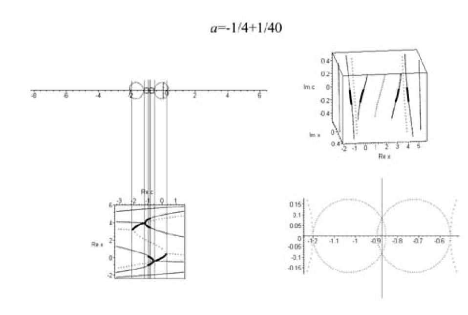
Figure 12: Domains of the orders $p=1,2$ of the Mandelbrot set ${\cal M}_{2,3}(a)$ at $a=-1/4+1/40=-0.225$, soon after the two descendant domains $(2,1)_{\pm}$ touched at $a=-0.2229529645\ldots$. Two order-$2$ orbits are simultaneously stable in the close vicinity of $c=-0.88$. Again, nothing special happens to the orbits themselves when the overlap occurs.

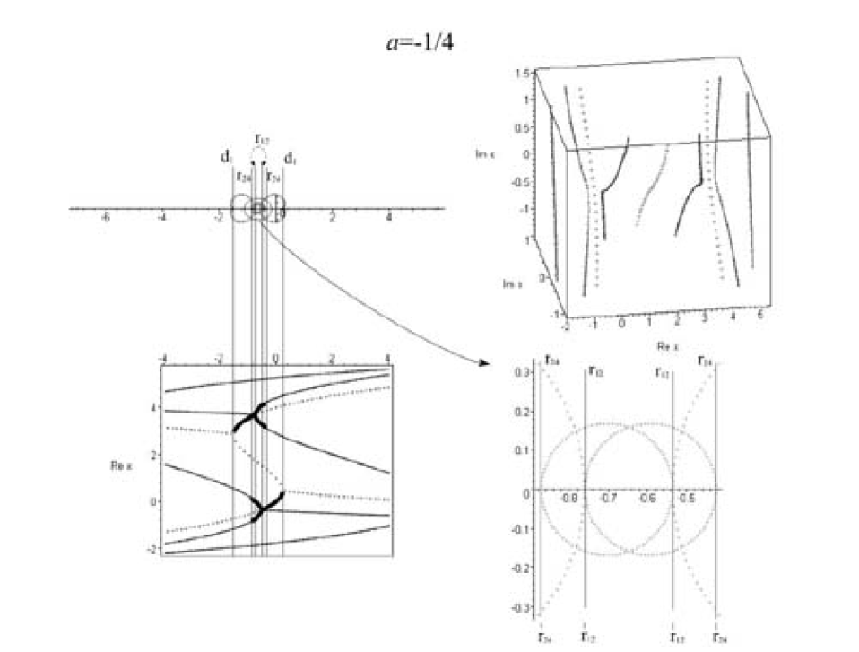
Figure 13: Domains of the orders $p=1,2$ of the Mandelbrot set ${\cal M}_{2,3}(a)$ at $a=-1/4$. The overlap increases, and now the descendant $(2,1)_{\pm}$ domains overlap not only each other, but also the twin parent $(1)_{\mp}$ domains. This means that in the vicinity of $c=-0.65$ there are two coexisting stable orbits of order $2$, while in the vicinities of $c=-0.5$ and $c=-0.8$ coexisting are stable orbits of orders $2$ and $1$. Nearly cusp-like behavior of the orbits in Julia-sheaf view in the upper right corner occurs in the vicinity of the zeroes $r_{12}$ of the resultant $R_{12}$, where the orbits of order two cross those of order one and the $(2,1)_{\pm}$ domains are attached to their parent $(1)_{\pm}$ domains. This singular behavior has nothing to do with the overlap of the domains.

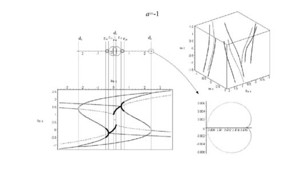
Figure 14: Domains of the orders $p=1,2$ of the Mandelbrot set ${\cal M}_{2,3}(a)$ at $a=-1$. The overlap increased even further as compared to Figs.12 and 13. Descendant domains $(2,1)_{\pm}$ now passed through the root ones $(1)_{\mp}$ and are no longer involved in the overlap. Instead overlapping are the root domains $(1)_{\pm}$ and two stable orbits of order $1$ coexist in the vicinity of $c=0$. If $(1)_{\pm}$ domains continued to move in the same direction with further increase of $|a|$, the two order $1$ orbits would cross (when the two zeroes $d_{1}^{\pm}$ of discriminant $D_{1}$ merge), and overlap would finally end in a collision – like it happens for positive values of $a$, see Fig.16. However, the merging of $D_{1}$ zeroes occurs at complex values $a=-\frac{1\pm i\sqrt{3}}{2}$, and at $a=-1$ the overlap is the biggest possible for real negative values of $a$. As $a$ decreases further (and $|a|$ grows) along the real-$a$ line, the $(1)_{\pm}$ domains start to move in the opposite direction, see Fig.15. We pass again through the overlap patterns like Fig.13 (at $a=-4$) and Fig.12 (at $a=-4.(4)$) and finally come back to the no-overlap pattern like Fig.9 (at $a=-10$) – all this in accordance with the symmetry (4.5).

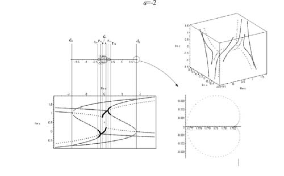
Figure 15: Domains of the orders $p=1,2$ of the Mandelbrot set ${\cal M}_{2,3}(a)$ at $a=-2$. The overlapping clusters start to diverge after maximal approach at $a=-1$, stopping short from collision of two zeroes of discriminant $D_{1}$, which would unify two clusters into a single one This actually happens at complex values of $a=\frac{1\pm i\sqrt{3}}{2}$, and we will enconter this unified cluster in our travel along real-$a$ axis, but at positive values of $a$.

4.1.3 Colliding domains

We left evolution in the positive-$a$ direction at the stage of Fig.11, when overlap of the two root domains $(2)_{\pm}$ just occured. In variance with the case of negative $a$, this time as the overlap increases the two zeroes $d_{2}$ of discriminant $D_{2}$, defining positions of the cusps of these two domains, coincide at $a=4-\sqrt{15}=0.12701665\ldots$ and a new phenomenon takes place. The two stable order-$2$ orbits (they were simultaneously stable in the overlap region) cross each other, and the pattern of orbits around crossing is pretty sophisticated, see Fig.16. Most interesting is preservation of two small overlap sections, where two different stable order-$2$ orbits continue to coexist, but exhibit non-trivial monodromy under a travel in the complex-$c$ plane around the cusps at zeroes of discriminant $D_{2}$.

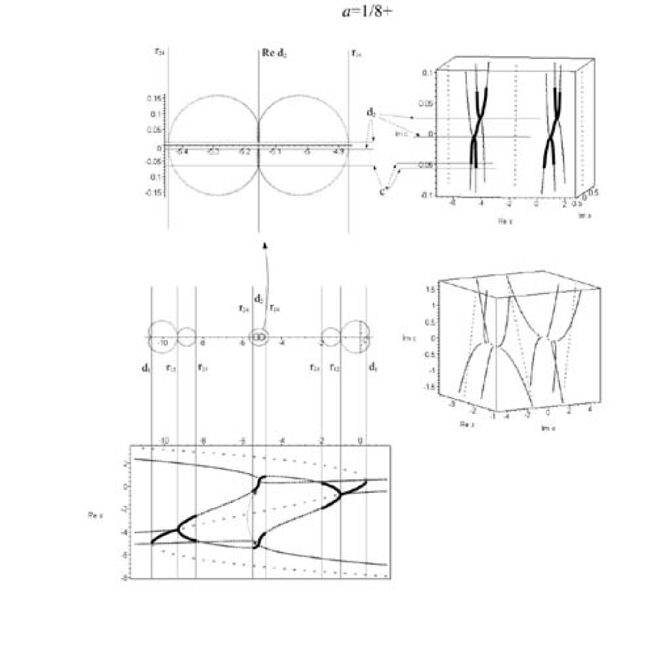
Figure 16: Domains of the orders $p=1,2$ of the Mandelbrot set at $a=1/8+1/224=0.12946(428571)$. The two root domains $(2)_{+}$ and $(2)_{-}$ just collided at $a=4-\sqrt{15}=0.12701665\ldots$ (after a period of overlap, originated at $a=0.1163898556\ldots$, see Fig.11), and their clusters are already united into a single new cluster, so that the union of $(2)=(2)_{+}\cup(2)_{-}$, $(2)_{+}\cap(2)_{-}\neq$, is now the new root domain. Arrows in the picture at the low left corner show the action of evolution $x\rightarrow f(x)$ on the points of the order-$2$ orbit. Enlarged picture in the left upper corner shows in more detail the new root cluster $(2)$. It has two narrow regions of self-overlap along the ${\rm Re}(c)={\rm Re}(d_{2})$ vetical axis, where two different order $(2)$ orbits are simultaneously stable. In all other points of the $(2)$ cluster only one order $2$ orbit is stable, but non-trivial monodromy occurs when we go around the cusps at $d_{2}^{\pm}={\rm Re}(d_{2})\pm{\rm Im}(d_{2})$ (points $D$): if we pick up the single stable order-$2$ orbit, say, at $c={\rm Re}(d_{2})$ (point $O$) and carry it into the upper overlap region from the right (counter-clock-wise), we obtain one of the two orbits, stable in that region, but if we carry the same orbit into the same region from the left (clock-wise), we obtain another stable orbit. If we continue to carry our orbits in the same direction and leave the overlap domain, the orbits loose stability. In other words, the two stable orbits in the overlap domain are permuted when carried around the cusp, and each orbit continues to be stable outside the overlap domain only if it is carried away in one out of two possible directions: either to the right or to the left. Another end of the overlap domain (point $E$), which is on the boundary of the $(2)$ cluster is not a cusp and not a singularity. As any point on the boundary of an elementary domain it has in its infinitesimal vicinity an infinite number of zeroes of various resultants $R_{2,2m}$, where the stable order-$2$ orbit exchanges stability with some order $2m$ orbit, see [2]. However, the set of relevant $\{m\}$ changes irregularly as we move along the boundary, and accordingly, for the point $E$ this set depends irregularly on $a$.

4.1.4 Colliding clusters

After collision of two root $(2)_{\pm}$ domains and formation of a unified cluster with the root $(2)$, the two other clusters, growing from the $(1)_{\pm}$ roots, continue to move towards each other and soon collide with the $(2)$ cluster, sandwiched in between them. Now this is indeed a collision, not just overlap, and, in variance with collision of the $(2)_{\pm}$ domains it now originates at the highest leaves (at $p=\infty$) rather than at the root domains. Full description of this process is impossible with the knowledge about the $p=1,2$ orbits only, thus our illustrations will be necessarily incomplete. Still, a lot is seen even with these limited tools.

Immediately after collision of the $(2)_{\pm}$ domains in Fig.16 they begin growing and soon become comparable in size with the $(2,1)_{\pm}$ domains, belonging to approaching clusters. Even earlier the overlapping region inside $(2)$ shrinks down and disappears. Finally, when the zeroes $r_{24}$ of the resultant $R_{24}$, marking the closest points of the $(2)$ and $(2,1)_{\pm}$ domains, coincide, collision wave, going down from the upper leaves of the clusters, reach the $p=2$ level: cluster collision gets seen at the level of our consideration. This happens at $a=0.1497297977\ldots$, see Fig.17. Figs.18 and 19 show Mandelbrot sets soon after that and a little later, when continuing approach of $(1)_{\pm}$ domains (which are now two roots of a single cluster!) starts pushing the unified $(2,1)$ domain outside of the region between them. This push-away process leads to the next bifurcation at $a=\frac{5-\sqrt{21}}{2}=0.20871215\ldots$ where the two zeroes $r_{12}$ of another resultant $R_{12}$ coincide, marking collision of the $(1)_{\pm}$ domains: collision wave reached the $p=1$ level. At this moment the $(2)$ cluster is ripped into two disconnected pieces, see Fig.20. Clearly, just the same push-away and ripping processes took place with all the higher-order domains $(2^{k},2^{k-1},\ldots,2,1)$ in between the moment of clusters collision till it reached the $p=2$ level at $a=0.2087\ldots$

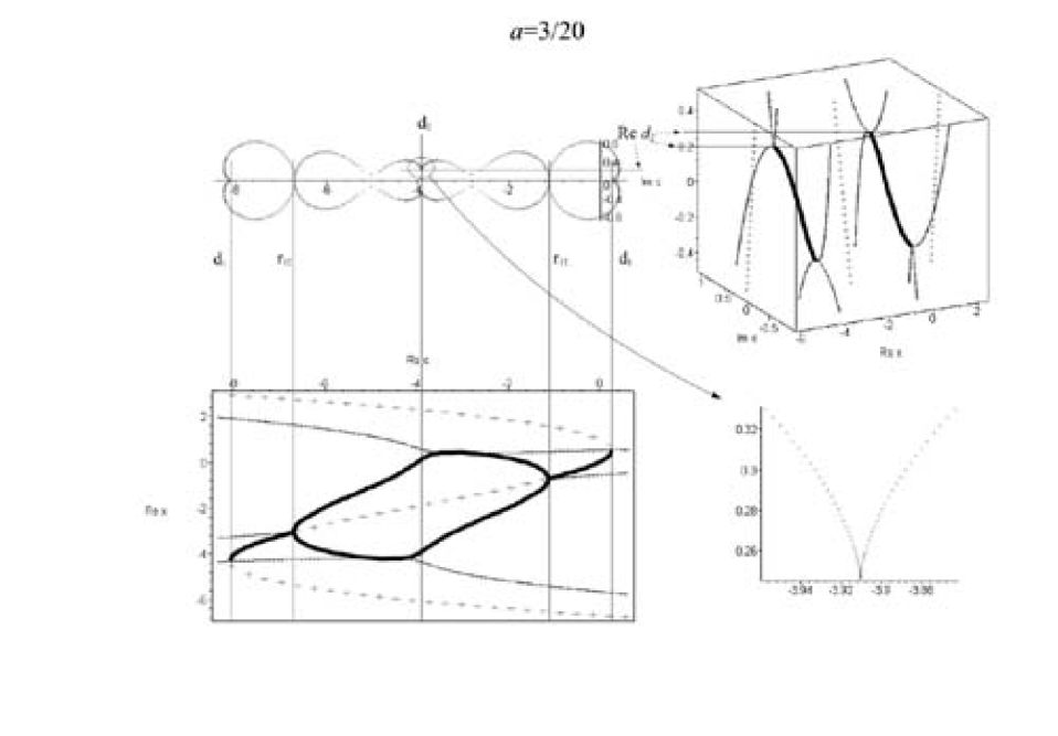
Figure 17: Domains of the orders $p=1,2$ of the Mandelbrot set ${\cal M}_{2,3}(a)$ at $a=3/20=0.15$. The $(2)$ domain just merged with the $(2,1)_{\pm}$ at $a=0.1497297977\ldots$ to form a single descendant $(2,1)$ domain. This unified domain has a characteristic four-sausage structure, remembering about its recent formation from four distinct elementary domains $(2)_{\pm}$ and $(2,1)_{\pm}$.

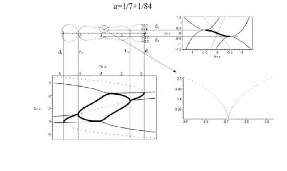
Figure 18: Domains of the orders $p=1,2$ of the Mandelbrot set ${\cal M}_{2,3}(a)$ at $a=1/7+1/84=0.15(476190)$. The shape of the unified $(2,1)$ domain evolved from the four-sausage to a two-sausage one: the memory about the difference between the $(2)$ and $(2,1)$ domains is almost erased, but distinction between $+$ and $-$ is still preserved.

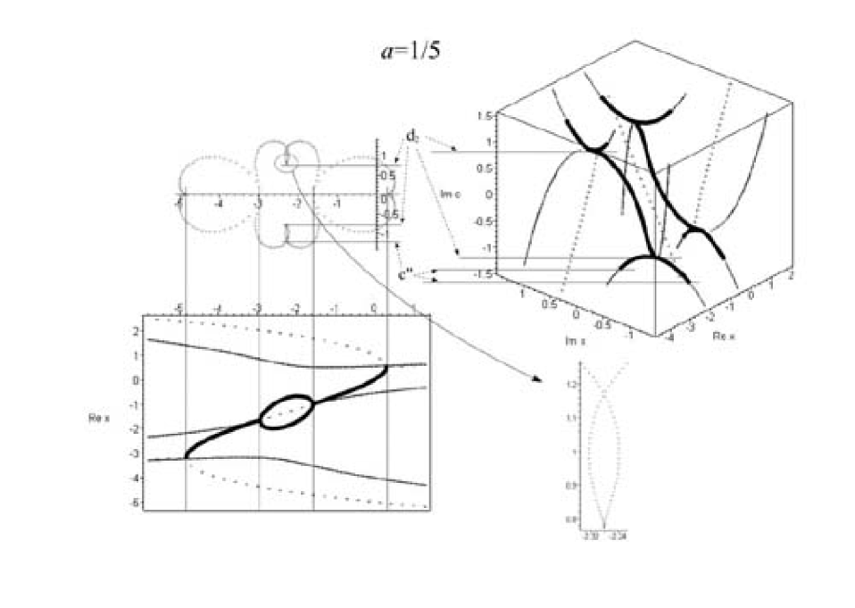
Figure 19: Domains of the orders $p=1,2$ of the Mandelbrot set ${\cal M}_{2,3}(a)$ at $a=1/5=0.2$. The $(2,1)$ domain is being pressed away by approaching $(1)_{\pm}$ domains, which are now the two roots of a single cluster. Note re-appearance of the narrow overlap regions inside the $(2,1)$ domain and non-trivial monodromy of the order $2$ orbits when they are carried along a circle in the Mandelbrot set, surrounding one of the cusps $d_{2}^{\pm}$.

4.1.5 Mandelbrot sets with the topology of ${\cal M}_{3}$ (in the vicinity of $a=1$)

The further evolution of ${\cal M}_{2,3}(a)$ with increasing $a$ consists mostly of continuous deformation of the shape of emerged unified root $(1)$ domain with two cusps: from a bone-like region in Fig.20 it grows into nearly oval one (deviating from oval only near the cusps) in Figs.21, 22 and finally at $a=1$, when the cusps extend their region of influence, acquires the standard form of Fig.23, familiar from Fig.2.

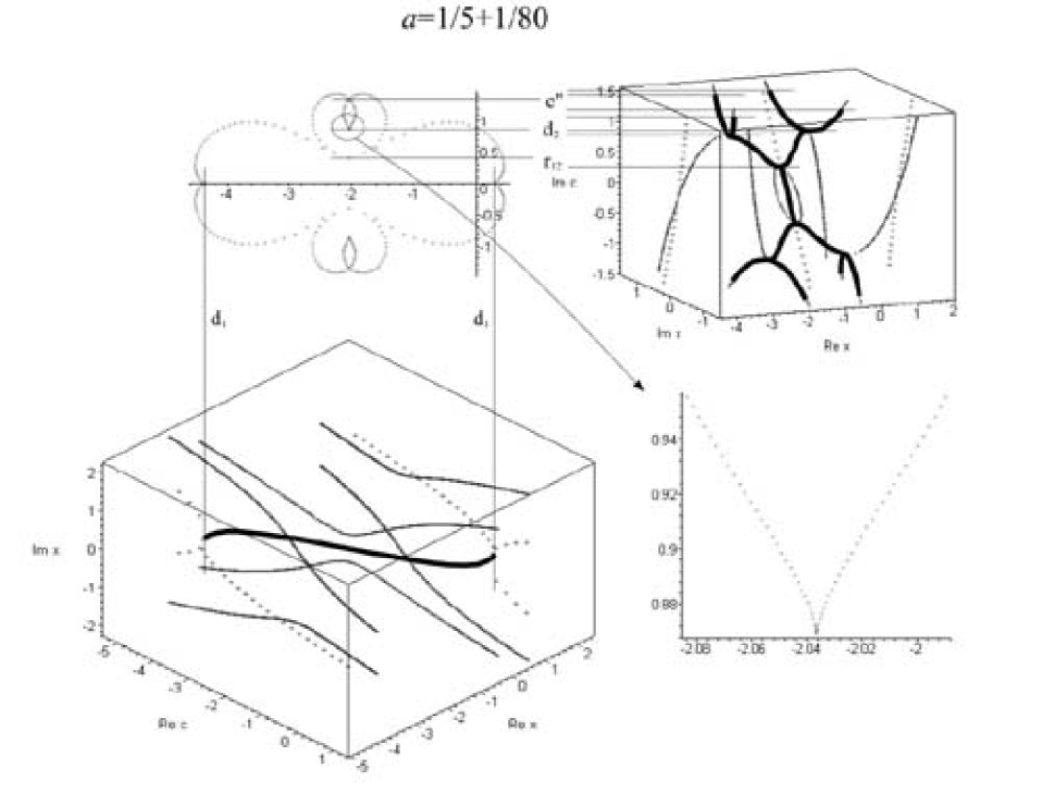
Figure 20: Domains of the orders $p=1,2$ of the Mandelbrot set ${\cal M}_{2,3}(a)$ at $a=1/5+1/80=0.2125$. The two root domains $(1)_{\pm}$ just collided at $a=\frac{5-\sqrt{21}}{2}=0.20871215\ldots$ and formed a single root domain $(1)$. It has a typical bone-like shape, with two pieces of the former descendant $(2,1)$ domain attached at the merging point. Overlap regions inside these $(2,1)_{\pm}$ fragments are now pretty large and cusps are not well seen, still the picture in the low right corner shows that they are still there. $3_{R}d$ view in the low left corner is taken at ${\rm Im}(c)=0$, where only order $p=1$ orbit can be stable inside the root $(1)$ domain.

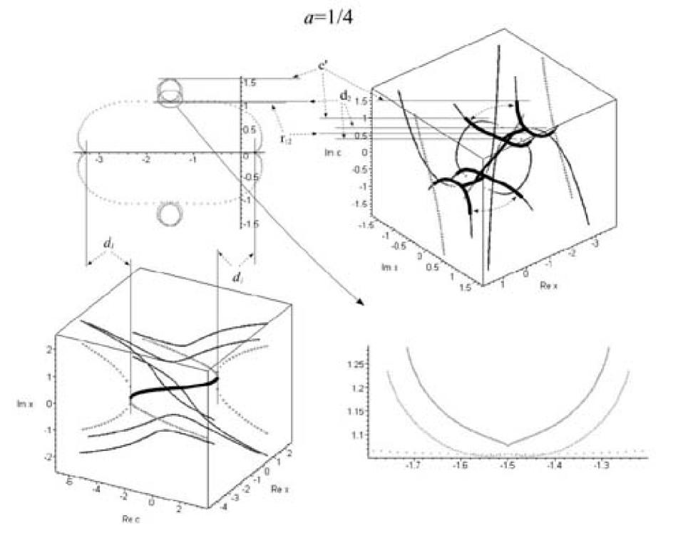
Figure 21: Domains of the orders $p=1,2$ of the Mandelbrot set ${\cal M}_{2,3}(a)$ at $a=1/4$. In this picture we are near the point $a=\frac{9-\sqrt{65}}{4}=0.23443556\ldots$ where inside-out reshuffling of the $(2,1)$ domains takes place (two zeroes $r_{24}$ of $R_{24}$ coincide at this transition point). Overlap regions, seen in Fig.20, grew up to the full size of the $(2,1)$ domains, and boundaries of the regions changes roles with boundaries of the domains. Later the former boundary domains will get closer and form new small overlap regions in Fig.22 that will later disappear at $a=0.42\ldots$

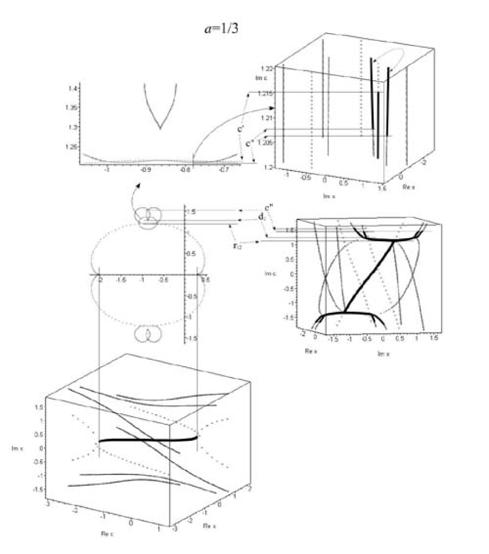
Figure 22: Domains of the orders $p=1,2$ of the Mandelbrot set ${\cal M}_{2,3}(a)$ at $a=1/3$. The root $(1)$ domain acquired an almost ellipsoidal form (outside the cusp regions). The interesting phenomenon, seen already in Fig.21, is appearance of additional overlap regions, marked by arrows in the upper left corner: between the root $(1)$ and descendant $(2,1)_{\pm}$ domains, where order-$1$ and order-$2$ orbits are simultaneously stable. This time there is no interesting monodromy: when we leave the overlap region in the direction of $(1)$ the order-$1$ orbit remains stable, when we go deep into $(2,1)_{\pm}$, the stable one is an order-$2$ orbit.

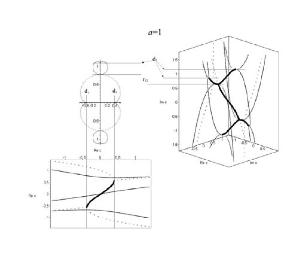
Figure 23: Domains of the orders $p=1,2$ of the Mandelbrot set ${\cal M}_{2,3}(a)$ at $a=1$. This is the central part of the standard Mandelbrot set ${\cal M}_{3}$, shown in Fig.2. All overlap regions disappeared, the $(1)$ domain is ideal cubic cardioid, other elementary domains acquire nearly cardioid shapes.

Still, while nothing equally drastic happens after the cluster collision, evolution is not quite event-less. In above pictures one can see that the overlap regions in the $(2,1)$ domain(s) appear and disappear, signaling about the motion of orbits in Julia sheaf with the change of $a$. In particular, an interesting inside-out reshuffling is shown in Fig.21. Moreover, in Fig.22 one can see that overlap occurs even between the $(1)$ and $(2,1)$ domains. We emphasize once again, that no bifurcations (phase transitions, orbit crossing or reshuffling) are associated with the overlaps, still they affect the shape and even the very presentation of the Mandelbrot set (when overlaps exist, it is not a clever idea to draw it all in black, like we did in Figs.1-4) and in fact this is a signal that the phase portrait gets richer: a non-trivial pattern of attractors and repulsers occurs, nothing to say that the vicinities of unstable orbits are not necessarily attracted to infinity, as implicitly assumed in some algorithms, mentioned in the first paragraphs of s.4.

Events, encountered in the evolution of Mandelbrot set ${\cal M}_{2,3}(a)$ from $a=0$ to $a=1$, i.e. in interpolation between Figs.1 and 2, are collected in the following table:

$a$ typical feature picture $a<0$ $\ldots$ $a=0$ the standard Mandelbrot Set ${\cal M}_{2}$ Fig.1 $0<a<0.1164\ldots$ two root domains of type $(1)$; Fig.8 two descendant domains $(2,1)$, attached to them; two isolated root domains $(2)$; two $(4,2,1)$ domains and two $(4,2)$ domains, attached to $(2,1)$ and $(2)$ at real values of $c$ $a=0.1164\ldots$ projections of two domains $(2)$ meet, i.e. two zeroes of $R_{24}$ coincide, responsible for stability of two different order-$2$ orbits $0.1164\ldots<a<0.1270\ldots$ projections of two domains $(2)$ overlap; two stable order-$2$ orbits coexist Fig.11 in the region of overlap $a=4-\sqrt{15}=0.1270\ldots$ cusps of overlapping domains $(2)$ merge, i.e. two zeroes of $D_{2}$ coincide $0.127\ldots<a<0.130\ldots$ overlap of the two domains $(2)$ Fig.16 splits into two isolated components $a=0.130\ldots$ overlap region shrinks down $0.130\ldots<a<0.1497\ldots$ only one unified root domain $(2)$ exists $a=0.1497\ldots$ $(2,1)$ domains merge with the $(2)$ domain, Fig.17 i.e. two pairs of zeroes of $R_{24}$ coincide, each pair responsible for stability of the same order-$2$ orbit $0.1497\ldots<a<6.6800\ldots$ only one $(2,1)$ domain exists; Fig.18 no $(2)$ domains $a=0.1875\ldots$ coexisting stable order-$2$ orbits re-emerge Fig.19 $a=\frac{5-\sqrt{21}}{2}=0.2087\ldots$ two $(1)$ domains meet and Fig.20 the $(2,1)$ domain splits into two, two zeroes of $R_{12}$ coincide $0.2087\ldots<a<0.42\ldots$ overlap regions, where two stable order-$2$ orbits Figs.21 & 22 or order-$2$ and order-$1$ orbits can coexist; $0.2087\ldots<a<4.7916\ldots$ one $(1)$ domain; two attached $(2,1)$ domains; no $(2)$ domains a = 0.42… overlap region shrinks down $a=1$ the standard Mandelbrot set ${\cal M}_{3}$ Figs.23 & 2 $a>1$ $\ldots$

In s.4.1.2 we briefly discussed what happens beyond the realm of this table: for negative values of $a$. The evolution of ${\cal M}_{2,3}(a)$ can be also continued to the region where $a>1$ (where $b=a-1<0$). This evolution appears to be reverse of what we already considered: the Mandelbrot set of Fig.2 at $a=1$ passes through the same stages of Figs.22, 21, 20 (at $a=3,\ 4,\ 4.706\ldots$ respectively) and so on. In particular, at $a=\frac{5+\sqrt{21}}{2}=4.7912878\ldots$ the single root $(1)$ domain is split into two, while two descendant $(2,1)$ domains merge into one. For illustration we show in Fig.24 the counterpart of Fig.19. The full picture will be shown in s.4.2 below.

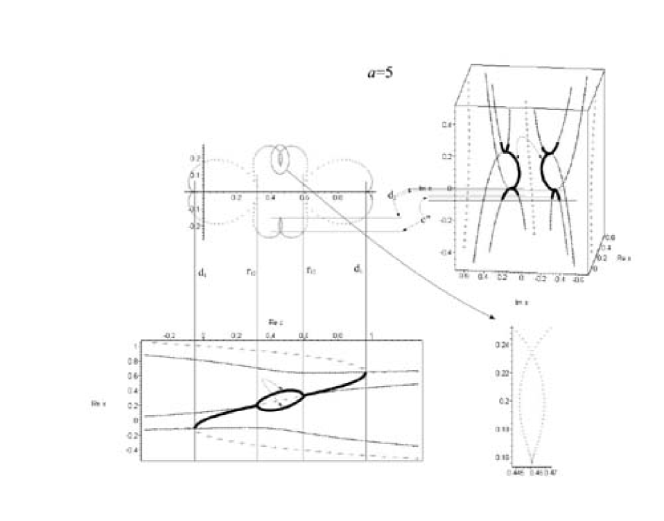
Figure 24: Domains of the orders $p=1,2$ of the Mandelbrot space ${\cal M}_{2,3}(a)$ at $a=5$. This picture is direct analogue of Fig.19, and serves as an illustration of the symmetry property (4.5): that the same sequence of bifurcations happens to the Mandelbrot set ${\cal M}_{2,3}(a)$ on the way from $a=1$ to $a=-1$ along the real-$a$ line through $a=\infty$ as on direct way, presented in Figs.8–23.

4.2 First steps towards UMS

Let us now return to interpretation of Mandelbrot sets as sections of a single Universal Mandelbrot Set (UMS). It implies that all what we observe about particular collection of Mandelbrot sets, like our one-parameter family ${\cal M}_{2,3}(a)$, can be re-interpreted as result of particular view on one and the same solid structure: variation of patterns is result of the changing view, the structure is always the same..

For example, the entire collection of the $p=1$ domains in Figs.8-24 which consist of a single component for $a$ in between $\frac{5\mp\sqrt{21}}{2}$ and split into two components outside this segment, see Fig.25.A, can be alternatively described as the image of a single cardioid-like domain in the slices, evolving with the change of the section in Fig.25.B. Moreover, in this approach one can even start from an ordinary circle, not from a cardioid, see Fig.26. In fact these pictures are nothing but approximate drawings, attempting to capture the properties of exact formula

$$c=-\frac{b}{3a}\left(1+\frac{2b^{2}}{9a}\right)\pm\left(1+\frac{2b^{2}}{9a}-\frac{e^{i\theta}}{3}\right)\frac{\sqrt{b^{3}+3ae^{i\theta}\phantom{5^{5^{5}}}}}{3a},$$ (4.6)

just now we interpret it is an evolution of (degenerate) elliptic mappings

$$(c-c_{0})^{2}=k(u-u_{1})(u-u_{2})(u-u_{3}),\ \ \ {\rm with}\ a-{\rm dependent\ parameters}\ c_{0},k\ {\rm and}\ u_{i};\ \ {\rm actually}\ u_{2}=u_{3}$$ (4.7)

of a complex-$u$ plane with a unit circle on it into a complex-$c$ plane, where the image of the unit circle looks differently: like our $p=1$ domains, evolving and even bifurcating (splitting and merging) under the change of the mapping.

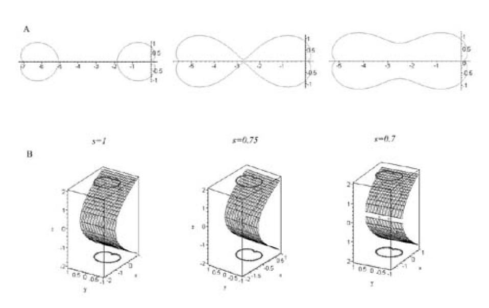
Figure 25: A. The shapes of $p=1$ elementary domains for different values of $a$ in the family $ax^{3}+(1-a)x^{2}+c$, as given by eq.(4.6).  B. The same (qualitatively) pictures arise in the sections of a single cardioid-like cylinder by different parabolic-like sections ($x-(z^{2}/2-s)=0$ for various $s$) with a complex-$c$ plane.   C. The cylinder can be even made circlic??? with the help of the circle-cardioid relation shown in Fig.26. The corresponding sections are now generic conics (quadrics???), not obligatory paraboloid. The true sections behind eq.(4.6) are cubic, see (4.7), not a quadric, which are a little less convenient to draw.

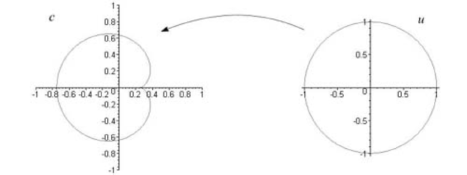
Figure 26: Cardioid cylinder of the previous Figure 25 can be substituted by an ordinary rotation-symmetric cylinder at expense of a more sophisticated slicing. Cardioid as a square of a circle. Analytically this correspondence is represented by $c=\frac{u}{2}\left(1-\frac{u}{2}\right)$ or $1-4c=(u-1)^{2}$.

At this early stage of investigation of UMS it is unclear, what is its best and simplest possible representation. In particular, nothing as simple as Fig.25 is immediately available when the order-$2$ orbits are taken into account. Therefore, instead of playing with different realizations, we show in Figs.27, 28 the most straightforward views of the Universal Mandelbrot Set, directly in the $a-c$ coordinates. Unfortunately, only $3_{R}$-dimensional section of the full $2_{C}$-dimensional pattern can be drawn in a picture and it can be rotated (what is very informative!) only on computer screen, see [6] for details about this option.

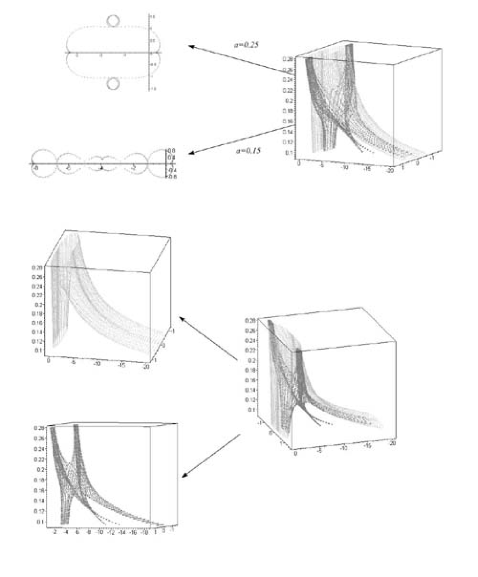
Figure 27: Collection of order-$1$ and -$2$ domains of Mandelbrot sets ${\cal M}_{2,3}(a)$ for the family $f(x)=ax^{3}+(1-a)x^{2}+c$ with various values of $a$ in the region $0.10\leq a\leq 0.28$, where most bifurcations are taking place, represented as slices of a single $3_{R}d$ entity, which can be also considered as a $3_{R}d$ section of UMS. Horizontal is the plane of complex $c$, vertical is the line of real $a$. This picture provides a concise summary of all the properties, described throughout s.4.1. The lower part of the figure represents separately the $p=1$ and $p=2$ domains: all pictures are also shown from different angles, what can help to appreciate the beauty of the structure.

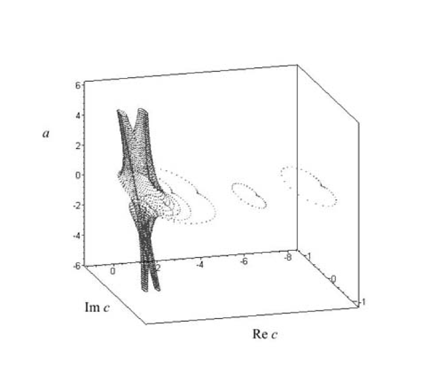
Figure 28: The same collection of Mandelbrot sets ${\cal M}_{2,3}(a)$ for the family $f(x)=ax^{3}+(1-a)x^{2}+c$ with all real values of $a$ (including those represented in Figs.8-24). Only central domains of order $1$ are shown.

In Fig.29 we give some more examples of $2_{C}$-sections of the UMS. In particular, we demonstrate that topologies of this section can be very different and they can be investigated by already available tools. As a small illustration, the chain of pictures in Fig.29,B shows how a loop in particular section of the UMS can be (on Fig.29,A) contracted. Of course, we are very far from calculation of homologies of the UMS, but the way is already open.

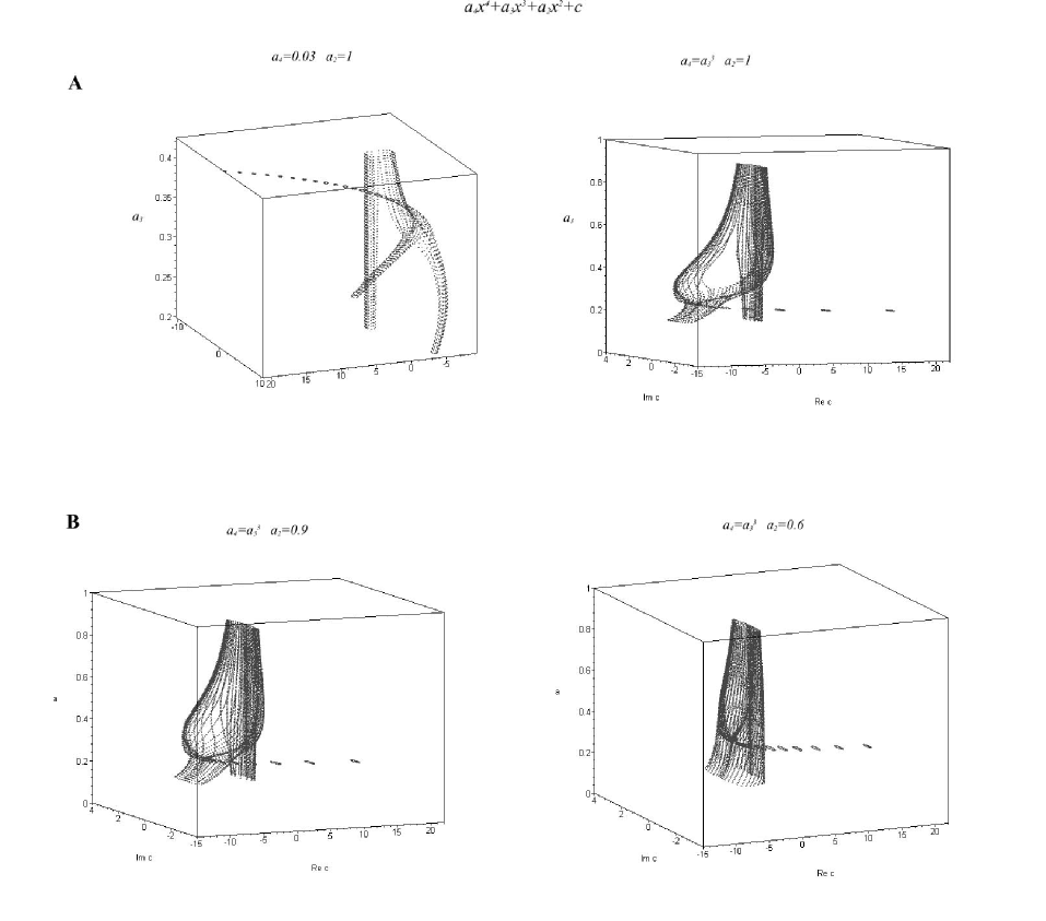
Figure 29: Examples of other $3_{R}d$ sections of the Universal Mandelbrot Set. Only central domains of order $1$ are shown.

5 Small-size approximation (SSA)

We now switch from transparent exact results to subtle approximate methods.

5.1 On status of the SSA

The shape of elementary domains can be also considered in the ”small-size” approximation (see s.4.9.3 of [2] and its less accurate predecessor in [8] and many other text-books). In SSA we expand all functions of $x$ and $c$ in powers of their deviations from the critical (or, simply, mean) values and leave only the first three (constant, linear and the next) terms in these expansions. In what follows $x_{cr}=0$, but $c_{cr}$ will have different values. ”Next” normally means quadratic, but for homogeneous polynomials $P_{d}(x)=x^{d}$ (giving rise to $Z_{d-1}$-symmetric Mandelbrot sets) it will actually mean $x^{d}$.

SSA would be very natural, if typical deviations of $x$ and $c$ from the mean values were small. However, while it can seem reasonable for the study of elementary domains – except for the first few, they are indeed pretty small in the $c$-plane (most are not even seen in Figs.1–3),– actually this assumption is wrong: as we already know from Figs.8–24, the $x$-variables in solutions to eqs.(2.3) are not small. At today’s level of knowledge justification of SSA comes only a posteriori, say, from comparison with experimental data in s.6). SSA seems adequate for phenomenological description of experimentally observed [7, 5] self-similarity (fractal or scaling) property of the Mandelbrot sets, but no clear theoretical reason for this adequateness is known. The algebro-geometrical approach of [2] only adds to the mystery: the (experimentally) obvious scaling properties of the universal discriminantal variety call for clear conceptual explanations.

In any case, today SSA is the only available approach to evaluation of Feigenbaum indices and other characteristics of elementary domains when their order $p\rightarrow\infty$. Surprisingly or not, it does a very good job in this field: see s.8 below.

5.2 SSA for the Mandelbrot Set

The first step of the SSA in application to the Mandelbrot Set (i.e. to the family $f(x;c)=x^{2}+c$) is to expand

$$F_{p}(x)=f_{p}(c)-x+x^{2}\gamma_{p}(c)+O(x^{4})$$ (5.1)

It is used here that that $f^{\prime}(x=0)=0$, otherwise expansion in powers of $x$ should be substituted by that in powers of $x-x_{cr}$, where $f^{\prime}(x_{cr})=0$.

The second step is to substitute (5.1) into (2.3). This gives:

$$2x\gamma_{p}(c)=e^{i\phi}$$ (5.2)

and

$$2f_{p}(c)\gamma_{p}(c)=2x\gamma_{p}(c)\Big{(}1-x\gamma_{p}(c)\Big{)}\ \stackrel{{\scriptstyle(\ref{xvsphi})}}{{=}}\ e^{i\phi}\left(1-\frac{1}{2}\,e^{i\phi}\right)$$ (5.3)

Eq.(5.3) provides the answer: the l.h.s. depends on the shape of the function $f(x;c)$, i.e. on $c$, and (5.3) describes a curve $c(\phi)$.

Actually this curve can have many disconnected components, and the third step is to consider a particular component, surrounding a particular root $c_{p}$ of the Mandelbrot function $f_{p}(c)=f(x_{cr},c)$:

$$f_{p}(c_{p})=0$$ (5.4)

Expand (5.3) around $c_{p}$:

$$c=c_{p}+\sigma,$$

$$f_{p}(c)=f_{p}(c_{p}+\sigma)=\dot{f}_{p}\,\sigma\left(1+\frac{\ddot{f}_{p}}{2\dot{f}_{p}}\,\sigma+O(\sigma^{2})\right)$$ (5.5)

$$\gamma_{p}(c)=\gamma_{p}(c_{p}+\sigma)=\gamma_{p}\left(1+\frac{\dot{\gamma}_{p}}{\gamma_{p}}\,\sigma+O(\sigma^{2})\right)$$

From now on we denote through $f_{p}$ and $\gamma_{p}$ the values of the corresponding functions at $c=c_{p}$: $\gamma_{p}\equiv\gamma_{p}(c_{p})$ etc. Substituting (5.5) into (5.3), we get:

$$\frac{\sigma}{r_{p}}\left(1-\frac{\xi_{p}}{2}\frac{\sigma}{r_{p}}\right)\approx r_{p}e^{i\phi}\left(1-\frac{1}{2}\,e^{i\phi}\right)$$ (5.6)

with

$$r_{p}=\frac{1}{2\dot{f}_{p}\gamma_{p}}$$ (5.7)

and

$$\xi_{p}=-\frac{1}{\dot{f}_{p}\gamma_{p}}\left(\frac{\ddot{f}_{p}}{2\dot{f}_{p}}+\frac{\dot{\gamma}_{p}}{\gamma_{p}}\right)$$ (5.8)

Eq.(5.6) is our final SSA answer for the shape of the elementary domain of the Mandelbrot Set, surrounding a point $c_{p}$. We see that the complex-valued $r_{p}$ defines the size and orientation of the domain, while its shape is fully controlled by the value of $\xi_{p}$: for $|\xi_{p}|\ll 1$ we get a cardioid, while for $|\xi_{p}-1|\ll 1$ it turns into a circle.

Thus our problem is reduced to:

– the check of accuracy of the small-size approximation:  we do this in s.6 by comparing the values of $r_{p}$, predicted by (5.7) with their actual values for the family $f(x;c)=x^{2}+c$, measured with the help of the Fractal Explorer [4] or defined from the roots of the relevant resultants;

– evaluation of parameter $\xi_{p}$ with the help of (5.8):   in s.7 we show that indeed in the small-size approximation $\xi_{p}=1$ for elementary domains, which are not roots of any clusters (i.e. are descendants of some lower-level domains);

– demonstration that higher-order cardioids emerge in the special case of maps with $Z_{d-1}$ symmetry: in this case the symmetry requires that $\gamma_{p}=0$ and (5.6) gets substituted by a more sophisticated expression (10.4), investigated in s.10 (emerging shapes are somewhat less ideal than for $d=2$, deviations can reach tens of percents).

5.3 Comments

Note that at the third step we kept terms up to $\sigma^{2}$ in expansions of the $c$-dependent functions, like we did at the first step with the $x$ functions. As usual for this type of method to work successfully it is important to correlate all approximations: attempt to make one part of calculation more accurate than another decreases the total accuracy. Note also that keeping linear terms only, without quadratic corrections, would make eq.(5.2) senseless, and according to the just formulated mnemonical rule one is forced to keep $\sigma^{2}$ terms as well. And indeed, neglecting them would provide a disaster in description of descendant domains: we already learned in s.2.5 that their characteristic difference from the root domains is that $\dot{F}_{p}(x,c)=\dot{f}_{p}(c)+x^{2}\dot{\gamma}(c)+O(x^{4})$ should vanish somewhere at the boundary, while in neglect of the $\sigma^{2}$ terms this would be very difficult to achieve while keeping $\dot{f}_{p}=\dot{f}_{p}(c_{p})\neq 0$ in the center $c_{p}$ of the domain. In fact, the difference between descendant and root domains is exactly in $\sigma^{2}$-terms: their relative magnitude is measured by parameter $\xi_{p}$, and it is negligibly small for root domains and close to unity for descendant ones.

6 On accuracy of the small-size approximation for the family $f=x^{2}+c$

Numerical characteristics of the lowest (in divisor forest) elementary domains of the Mandelbrot set ${\cal M}_{2}$ are represented in the following table (positions of these domains are marked by arrows in Fig.30).

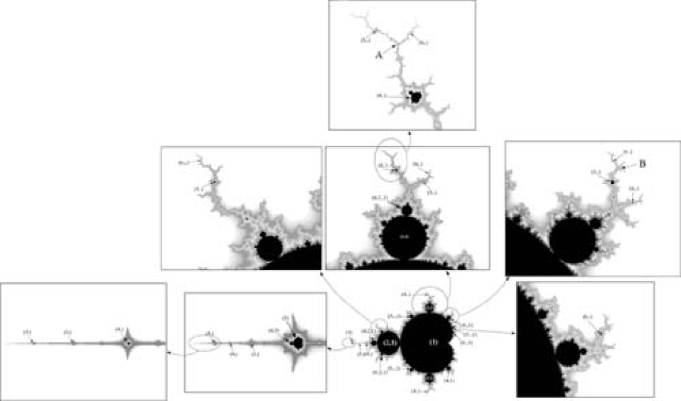
Figure 30: Mandelbrot Set from Fig.1 with arrows, pointing at particular elementary domains, represented in the table in s.6. Trails are also seen in pictures with increased resolutions. Trails are densely populated by clusters. The theory of trails remains an open subject. An interesting task is to study how a trail between some two clusters is formed, when we travel across Universal Mandelbrot Space as in s.4.1, and these two clusters emerge from a splitting of a single cluster. Another interesting problem is to find the locations of the crossing points, where many trails meet together, examples of such crossings are points ${\bf A}$ and ${\bf B}$.

$$\begin{array}[]{|c|c|c|c|c|c|c|c|c|}\hline\cr&&&&&&&&\\ p&1&2&3&3&4&4&4&4\\ &&&&&&&&\\ \hline\cr&&&&&&&&\\ c_{p}&0&-1&-1.754877667&-0.1225611669&-1.940799807&-0.1565201668&0.2822713908&-1.310702641\\ &&&&\pm 0.7448617670i&&\pm 1.032247109i&\pm 0.5300606176i&\\ &&&&&&&&\\ \hline\cr&&&&&&&&\\ {\rm distance}&{\bf 0}&{\bf 1}&{\bf 0}&{\bf 1}&{\bf 0}&{\bf 0}&{\bf 1}&{\bf 2}\\ {\rm from\ the\ root}&(1)&(2,1)&(3)&(3_{\pm},1)&(4_{1})&(4_{2\pm})&(4_{\pm},1)&(4,2,1)\\ &&&&&&&&\\ \hline\cr\hline\cr&&&&&&&&\\ \dot{f}_{p}&1&-1&-5.649435914&-1.67528205&-25.53361247&-9.826826127&-2.273407347&1.734079638\\ &&&&\mp 1.1245590i&&\mp 1.391722418i&\mp 2.878229429i&\\ &&&&&&&&\\ \hline\cr&&&&&&&&\\ \ddot{f}_{p}&0&2&17.89661552&-5.9483077&247.9985718&-13.82424296&-30.39333448&-15.56341649\\ &&&&\pm 6.7473541i&&\pm 86.41684550i&\mp 9.578562508i&\\ &&&&&&&&\\ \hline\cr&&&&&&&&\\ \gamma_{p}&1&-2&-9.29887185&-1.35056409&-39.49472178&-10.55453437&-0.142465954&4.88872230\\ &&&&\mp 2.249118i&&\mp 5.448066568i&\mp 3.098932717i&\\ \hline\cr&&&&&&&&\\ \dot{\gamma}_{p}&0&2&22.91612617&-7.458063&-39.49472178&-42.68642404&-14.72856928&-21.82510289\\ &&&&\pm 3.767907i&&\pm 80.90620560i&\mp 16.79943562i&\\ \hline\cr\hline\cr&&&&&&&&\\ \xi_{p}&{0}&{1}&{0.07706201109}&{1.0212516}&{0.01367007063}&{0.05842559742}&{1.011598455}&{1.055967271}\\ {\rm from}\ (\ref{xip})&&&&{\pm 0.04763015i}&&{\pm 0.08449808566i}&{\pm 0.07045065295i}&\\ &{\bf\ll 1}&{\bf=1}&{\bf\ll 1}&{\bf\approx 1}&{\bf\ll 1}&{\bf|\xi_{p}|\ll 1}&{\bf\approx 1}&{\bf\approx 1}\\ &&&&&&&&\\ \hline\cr&&&&&&&&\\ {\bf 2r_{p}}=(\dot{f}_{p}\gamma_{p})^{-1}&{\bf 1}&{\bf 0.5}&{\bf 0.0190355}&{\bf-0.009518}&{\bf 0.00099163}&{\bf 0.0069178}&{\bf-0.066394}&{\bf 0.1179602}\\ {\rm from}\ (\ref{diam})&&&&{\bf\mp 0.18867i}&&{\bf\mp 0.0049095i}&{\bf\mp 0.057585i}&\\ &&&&&&&&\\ \hline\cr\hline\cr&&&&&&&&\\ c_{p+}&0.25&-0.75&-1.75&-0.125&-1.940550789&-0.1547246055&0.25&-1.25\\ &&&&\pm 0.6495190528i&&\pm 1.031047228i&\pm 0.5i&\\ &&&&(=\pm 3\sqrt{3}i/8)&&&&\\ \hline\cr&&&&&&&&\\ c_{p-}&-0.75&-1.25&-1.768529153&-0.1157354238&-1.941537753&-0.1613575037&0.3161758500&-1.368098940\\ &&&&\pm 0.8379990280i&&\pm 1.036031085i&\pm 0.5574717760i&\\ \hline\cr&&&&&&&&\\ c_{p+}-c_{p-}&{\bf 1}&{\bf 0.5}&{\bf 0.018529153}&{\bf-0.0092645762}&{\bf 0.000986964}&{\bf 0.0066328982}&{\bf-0.0661758500}&{\bf 0.118098940}\\ &&&&{\bf\mp 0.1884799750i}&&{\bf\mp 0.004983857i}&{\bf\mp 0.057471776i}&\\ &&&&&&&&\\ \hline\cr&&&&&&&&\\ \kappa&{\bf 4}&{\bf 2}&{\bf 4}&{\bf 2}&{\bf 4}&{\bf 4}&{\bf 2}&{\bf 2}\\ (c_{p+}-c_{p})\kappa&{\bf 1}&{\bf 0.5}&{\bf 0.019510668}&{\bf-0.0048776662}&{\bf 0.000996072}&{\bf 0.0071822452}&{\bf-0.0645427816}&{\bf 0.121405282}\\ &&&&{\bf\mp 0.1906854280i}&&{\bf\mp 0.004799524i}&{\bf\mp 0.0601212352i}&\\ &&&&&&&&\\ \hline\cr\end{array}\hskip 17.07182pt$$

The entries in the last two rows should be both compared with $2r_{p}$, which is calculated within SSA in the middle part of the table. Since the shapes of root and descendant domains are different, parameters $\kappa$ in the last row are also different: $\kappa=4$ for cardioid-shape root domains and $\kappa=2$ for circle-shape descendant domains.

$$\begin{array}[]{|c|c|c|c|c|c|c|}\hline\cr&&&&&&\\ p&5&5&5&5&5&5\\ &&&&&&\\ \hline\cr&&&&&&\\ c_{p}&-1.625413725&-1.860782522&-1.985424253&0.3592592248&-0.04421235770&-0.1980420994\\ &&&&\pm 0.6425137371i&\pm 0.9865809763i&\pm 1.100269537i\\ &&&&&&\\ \hline\cr&&&&&&\\ {\rm distance}&{\bf 0}&{\bf 0}&{\bf 0}&{\bf 0}&{\bf 0}&{\bf 0}\\ {\rm from\ the\ root}&(5_{1})&(5_{2})&(5_{3})&(5_{4\pm})&(5_{5\pm})&(5_{6\pm})\\ &&&&[\ldots,8,4_{\pm},1]&[\ldots,12,6,3_{\pm},1]&[\ldots,12,6,3_{\pm},1]\\ &&&&&&\\ \hline\cr\hline\cr&&&&&&\\ \dot{f}_{p}&-12.346786&27.952811&-106.51134&-15.264582&-1.4606030&-34.451623\\ &&&&\mp 4.049590i&\mp 15.65788i&\pm 8.245915i\\ &&&&&&\\ \hline\cr&&&&&&\\ \ddot{f}_{p}&32.445339&-211.46971&3811.7679&-270.4039&-190.8108&421.6135\\ &&&&\pm 144.8293i&\mp 151.4911i&\pm 736.0759i\\ &&&&&&\\ \hline\cr&&&&&&\\ \gamma_{p}&-19.95443&45.84473&-161.34688&-9.4954135&6.050675&-41.054355\\ &&&&\mp 9.112127i&\mp 17.26642i&\mp 3.02090i\\ &&&&&&\\ \hline\cr&&&&&&\\ \dot{\gamma}_{p}&17.8489&-272.6037&5625.2834&-237.5248&-108.0265&207.2558\\ &&&&\mp 0.045178i&\mp 230.0270i&\pm 911.8688i\\ &&&&&&\\ \hline\cr\hline\cr&&&&&&\\ \xi_{p}&{0.008963643}&{0.007591840}&{0.00306997}&{0.02825982}&{0.03863736}&{0.00311728}\\ {\rm from}\ (\ref{xip})&&&&{\pm 0.1305419i}&{\mp 0.06450516i}&{\pm 0.02358242i}\\ &{\bf\ll 1}&{\bf\ll 1}&{\bf\ll 1}&{\bf|\xi_{p}|\ll 1}&{\bf|\xi_{p}|\ll 1}&{\bf|\xi_{p}|\ll 1}\\ &&&&&&\\ \hline\cr&&&&&&\\ {\bf 2r_{p}}=(\dot{f}_{p}\gamma_{p})^{-1}&{\bf 0.004058884}&{\bf 0.0007803423}&{\bf 0.0000581894}&{\bf 0.00250125}&{\bf-0.0033726}&{\bf 0.00067682}\\ {\rm from}\ (\ref{diam})&&&&{\bf\mp 0.00411026i}&{\bf\pm 0.00083981i}&{\bf\pm 0.00011025i}\\ &&&&&&\\ \hline\cr\hline\cr&&&&&&\\ c_{p+}&-1.624396989&-1.860586973&-1.985409691&0.3599331332&-0.04506136598&-0.1978729467\\ &&&&\pm 0.6415066668i&\pm 0.9868115622i&\pm 1.100298438i\\ &&&&&&\\ \hline\cr&&&&&&\\ \kappa&{\bf 4}&{\bf 4}&{\bf 4}&{\bf 4}&{\bf 4}&{\bf 4}\\ (c_{p+}-c_{p})\kappa&{\bf 0.004066944}&{\bf 0.000782196}&{\bf 0.000058248}&{\bf 0.0026956336}&{\bf-0.00339603312}&{\bf 0.0006766108}\\ &&&&{\bf\mp 0.0040282812i}&{\bf\pm 0.0009223436i}&{\bf\pm 0.000115604i}\\ &&&&&&\\ \hline\cr\end{array}$$

$$\begin{array}[]{|c|c|c|c|c|c|c|c|}\hline\cr&&&&&&&\\ p&5&5&5&6&6&6&6\\ &&&&&&&\\ \hline\cr&&&&&&&\\ c_{p}&-1.256367930&0.3795135880&-0.5043401754&-1.476014643&-1.907280091&-1.966773216&-1.996376138\\ &\pm 0.3803209635i&\pm 0.3349323056i&\pm 0.5627657615i&&&&\\ &&&&&&&\\ \hline\cr&&&&&&&\\ {\rm distance}&{\bf 0}&{\bf 1}&{\bf 1}&{\bf 0}&{\bf 0}&{\bf 0}&{\bf 0}\\ {\rm from\ the\ root}&(5_{7\pm})&(5_{1\pm},1)&(5_{2\pm},1)&(6_{1})&(6_{2})&(6_{3})&(6_{4})\\ &[\ldots,12,6_{\pm},2,1]&&&&&&\\ \hline\cr\hline\cr&&&&&&&\\ \dot{f}_{p}&-9.720195&-2.700383&-3.449207&9.557119&-73.91417&135.0997&-431.94389\\ &\mp 11.81330i&\mp 5.404227i&\mp 1.112266i&&&&\\ &&&&&&&\\ \hline\cr&&&&&&&\\ \ddot{f}_{p}&-59.44225&-48.15074&9.823111&-106.133658&491.1284&-2562.839&60341.247\\ &\pm 171.0187i&\mp 78.38748i&\pm 30.87527i&&&&\\ &&&&&&&\\ \hline\cr&&&&&&&\\ \gamma_{p}&-5.71067&0.809902&-2.871463&20.23824&-115.0273&207.856&-649.8852\\ &\mp 21.95456i&\mp 3.399590i&\mp 2.098768i&&&&\\ &&&&&&&\\ \hline\cr&&&&&&&\\ \dot{\gamma}_{p}&-165.8458&2.830436&0.04567&-150.6058&576.3060&-3609.262&90085.134\\ &\pm 183.4574i&\mp 47.49326i&\pm 29.22689i&&&&\\ &&&&&&&\\ \hline\cr\hline\cr&&&&&&&\\ \xi_{p}&{0.0176798}&{1.00083}&{0.984283}&{0.067182}&0.00098004&0.00095613&0.0007426\\ {\rm from}\ (\ref{xip})&{\mp 0.0451181i}&{\pm 0.0866142i}&{\mp 0.000539978i}&&&&\\ &{\bf|\xi_{p}|\ll 1}&{\bf\approx 1}&{\bf\approx 1}&{\bf\ll 1}&{\bf\ll 1}&{\bf\ll 1}&{\bf\ll 1}\\ &&&&&&&\\ \hline\cr&&&&&&&\\ {\bf 2r_{p}}=(\dot{f}_{p}\gamma_{p})^{-1}&{\bf-0.001692541}&{\bf-0.04612246}&{\bf 0.04556086}&{\bf 0.005170116}&{\bf 0.000117617}&{\bf 0.000035611}&{\bf 0.0000035623}\\ {\rm from}\ (\ref{diam})&{\bf\mp 0.00233202i}&{\bf\mp 0.0107757i}&{\bf\mp 0.0627926i}&&&&\\ &&&&&&&\\ \hline\cr\hline\cr&&&&&&&\\ c_{p+}&-1.256801994&0.3567627458&-0.4817627458&-1.47469537780&-1.90725067795&-1.96676431090&-1.99637524690\\ &\pm 0.3797412022i&\pm 0.3285819450i&\pm 0.5316567552i&&&&\\ &&&&&&&\\ \hline\cr&&&&&&&\\ \kappa&{\bf 4}&{\bf 2}&{\bf 2}&{\bf 4}&{\bf 4}&{\bf 4}&{\bf 4}\\ (c_{p+}-c_{p})\kappa&{\bf-0.0017363}&{\bf-0.04550168}&{\bf 0.04515486}&{\bf 0.00527706}&{\bf 0.000117652}&{\bf 0.000035620}&{\bf 0.000003564}\\ &{\bf\mp 0.00231905i}&{\bf\mp 0.01270072i}&{\bf\mp 0.06221801i}&&&&\\ &&&&&&&\\ \hline\cr\end{array}\hskip 28.45274pt$$

$$\begin{array}[]{|c|c|c|c|c|c|c|}\hline\cr&&&&&&\\ p&6&6&6&6&6&6\\ &&&&&&\\ \hline\cr&&&&&&\\ c_{p}&0.4433256334&0.3965345700&0.3598927390&-0.01557038602&-0.1635982616&-0.2175267470\\ &\pm 0.3729624167i&\pm 0.6041818105i&\pm 0.6847620202i&\pm 1.020497366i&\pm 1.097780643i&\pm 1.114454266i\\ &&&&&&\\ \hline\cr&&&&&&\\ {\rm distance}&{\bf 0}&{\bf 0}&{\bf 0}&{\bf 0}&{\bf 0}&{\bf 0}\\ {\rm from\ the\ root}&(6_{5\pm})&(6_{6\pm})&(6_{7\pm})&(6_{8\pm})&(6_{9\pm})&(6_{10\pm})\\ &[\ldots,10,5_{1\pm},1]&[\ldots,8,4_{\pm},1]&[\ldots,8,4_{\pm},1]&[\ldots,6,3_{\pm},1]&[\ldots,6,3_{\pm},1]&[\ldots,6,3_{\pm},1]\\ &&&&&&\\ \hline\cr\hline\cr&&&&&&\\ \dot{f}_{p}&-22.131316&-7.730347&-45.44965&-47.08247&-13.70794&-94.05752\\ &\mp 8.549589i&\mp 29.76415i&\pm 11.11460i&\mp 42.3870i&\mp 59.0423i&\pm 65.91697i\\ &&&&&&\\ \hline\cr&&&&&&\\ \ddot{f}_{p}&-868.64319&-427.073&-431.8717&-3003.383&-2600.199&7694.999\\ &\mp 90.27354i&\mp 1083.050i&\pm 2162.074i&\pm 437.063i&\mp 913.171i&\pm 2405.039i\\ &&&&&&\\ \hline\cr&&&&&&\\ \gamma_{p}&-8.156137&6.87116&-37.7109&-28.2862&7.68865&-125.4789\\ &\mp 11.41327i&\mp 23.4912i&\mp 9.24215i&\mp 64.5198i&\mp 69.5663i&\pm 40.9618i\\ &&&&&&\\ \hline\cr&&&&&&\\ \dot{\gamma}_{p}&-389.998&151.331&-1097.368&-3129.19&-2370.323&7560.924\\ &\mp 307.274i&\mp 866.959i&\pm 1391.979i&\mp 931.571i&\mp 1950.970i&\pm 5049.389i\\ &&&&&&\\ \hline\cr\hline\cr&&&&&&\\ \xi_{p}&0.00405&0.07215&-0.01588&0.014630&0.010020&-0.001788\\ {\rm from}\ (\ref{xip})&\pm 0.16159i&\mp 0.01058i&\pm 0.034629i&\pm 0.005837i&\mp 0.01208i&\pm 0.006621i\\ &{\bf|\xi_{p}|\ll 1}&{\bf|\xi_{p}|\ll 1}&{\bf|\xi_{p}|\ll 1}&{\bf|\xi_{p}|\ll 1}&{\bf|\xi_{p}|\ll 1}&{\bf|\xi_{p}|\ll 1}\\ &&&&&&\\ \hline\cr&&&&&&\\ {\bf 2r_{p}}=(\dot{f}_{p}\gamma_{p})^{-1}&{\bf 0.0007487}&{\bf-0.0013280}&{\bf 0.00055046}&{\bf-0.00007044}&{\bf-0.00023408}&{\bf 0.000039602}\\ {\rm from}\ (\ref{diam})&{\bf\mp 0.0029099i}&{\bf\pm 0.00004046i}&{\bf\mp 0.000000276i}&{\bf\mp 0.0002127i}&{\bf\mp 0.00002776i}&{\bf\pm 0.00005275i}\\ &&&&&&\\ \hline\cr\hline\cr&&&&&&\\ c_{p+}&0.44355069141&0.39619446067&0.3600296164&-0.01558797607&-0.163657003678&-0.217516881\\ &\pm 0.372246821i&\pm 0.60419336859i&\pm 0.684763498i&\pm 1.0204438975i&\pm 1.0977739136i&\pm 1.114467467i\\ &&&&&&\\ \hline\cr&&&&&&\\ \kappa&{\bf 4}&{\bf 2}&{\bf 2}&{\bf 4}&{\bf 4}&{\bf 4}\\ (c_{p+}-c_{p})\kappa&{\bf 0.000900232}&{\bf-0.001360437}&{\bf 0.00054751}&{\bf-0.000070360}&{\bf-0.000234968}&{\bf 0.000039463}\\ &{\bf\mp 0.00286238i}&{\bf\pm 0.00004623i}&{\bf\pm 0.00000591i}&{\bf\mp 0.00021387i}&{\bf\mp 0.00002692i}&{\bf\pm 0.00005280i}\\ &&&&&&\\ \hline\cr\end{array}$$

$$\begin{array}[]{|c|c|c|c|c|c|c|}\hline\cr&&&&&&\\ p&6&6&6&6&6&6\\ &&&&&&\\ \hline\cr&&&&&&\\ c_{p}&-0.5968916446&-1.284084926&0.3890068406&-1.772892903&-0.1134186559&-1.138000667\\ &\pm 0.6629807446i&\pm 0.4272688960i&\pm 0.2158506509i&&\pm 0.8605694725i&\pm 0.2403324013i\\ &&&&&&\\ \hline\cr&&&&&&\\ {\rm distance}&{\bf 0}&{\bf 0}&{\bf 1}&{\bf 1}&{\bf 2}&{\bf 2}\\ {\rm from\ the\ root}&(6_{11\pm})&(6_{12\pm})&(6_{\pm},1)&(6,3)&(6,3_{\pm},1)&(6_{\pm},2,1)\\ &[\ldots,10,5_{2\pm},1]&[\ldots,12,6_{\pm},2,1]&&&&\\ &&&&&&\\ \hline\cr\hline\cr&&&&&&\\ \dot{f}_{p}&-21.17430&-49.4808&-2.84507&6.02446709&2.710416&3.0373845\\ &\mp 1.239334i&\mp 43.51796i&\mp 8.81348i&&\pm 2.01496i&\pm 0.674370i\\ &&&&&&\\ \hline\cr&&&&&&\\ \ddot{f}_{p}&258.9018&-401.263&-13.2205&-699.2133940&53.81286&-9.154561\\ &\pm 390.3375i&\pm 2355.001i&\mp 228.2727i&&\mp 56.37906i&\mp 50.431515i\\ &&&&&&\\ \hline\cr&&&&&&\\ \gamma_{p}&-19.86933&-40.9497&1.51341&19.09634167&3.35657&3.882374\\ &\mp 7.65439i&\mp 85.4133i&\mp 3.51012i&&\pm 5.72766i&\pm 4.659455i\\ &&&&&&\\ \hline\cr&&&&&&\\ \dot{\gamma}_{p}&122.1821&-1796.0107&47.3746&-1106.4705637&71.1246&28.408033\\ &\pm 435.7183i&\pm 2809.8473i&\mp 74.1184i&&\mp 30.8637i&\mp 64.35131i\\ &&&&&&\\ \hline\cr\hline\cr&&&&&&\\ \xi_{p}&0.062667&0.005776&0.99288&1.00806&1.03542&1.0497\\ {\rm from}\ (\ref{xip})&\pm 0.034437i&\mp 0.006297i&\pm 0.09882i&&\pm 0.013004i&\pm 0.0438i\\ &{\bf|\xi_{p}|\ll 1}&{\bf|\xi_{p}|\ll 1}&{\bf\approx 1}&{\bf\approx 1}&{\bf\approx 1}&{\bf\approx 1}\\ &&&&&&\\ \hline\cr&&&&&&\\ {\bf 2r_{p}}=(\dot{f}_{p}\gamma_{p})^{-1}&{\bf 0.0020161}&{\bf-0.000043399}&{\bf-0.0281207}&{\bf 0.008692230}&{\bf-0.0048602}&{\bf 0.0242924}\\ {\rm from}\ (\ref{diam})&{\bf\mp 0.0009153i}&{\bf\mp 0.00015422i}&{\bf\pm 0.0026745i}&&{\bf\mp 0.044335i}&{\bf\mp 0.047098i}\\ &&&&&&\\ \hline\cr\hline\cr&&&&&&\\ c_{p+}&-0.5963742242&-1.284095877&0.375&-1.768529153&-0.1157354238&-1.125\\ &\pm 0.6627532528i&\pm 0.4272302898i&\pm 0.2165063509i&&\pm 0.837999027i&\pm 0.2165063509i\\ &&&&&&\\ \hline\cr&&&&&&\\ \kappa&{\bf 4}&{\bf 4}&{\bf 2}&{\bf 2}&{\bf 2}&{\bf 2}\\ (c_{p+}-c_{p})\kappa&{\bf 0.00206968}&{\bf-0.00004380}&{\bf-0.028013681}&{\bf 0.008727500}&{\bf-0.0046335357}&{\bf 0.0260013340}\\ &{\bf\mp 0.000909967i}&{\bf\mp 0.00015442i}&{\bf\pm 0.001311400i}&&{\bf\mp 0.045140890254i}&{\bf\mp 0.0476521007i}\\ &&&&&&\\ \hline\cr\end{array}$$

A few comments to the table are now in order:

We present the values of parameters with high accuracy, which strongly exceeds our needs in the present paper, but this data can be used in the future investigations. One should not be surprised by the high accuracy of experimental data: since it is computer experiment over Platonian entity, accuracy is unlimited. Moreover the numbers in the last column can be also reproduced as resultants zeroes [2]: though it is a difficult calculation (beyond capabilities of MAPLE on an ordinary laptop already for $p>6$), its accuracy is in principle unlimited.

$c_{+}$ is closer to the root than $c_{-}$: $c_{+}$ is the point of merging with the parent domain or the cusp position if the domain is itself a root, while $c_{-}$ is the ”opposite” point, i.e. the merging point with the next descendant of the order $2$.

Starting from $p=5$ there are many root domains of the type $(5)$, $(6)$ etc, and – starting from $p=3$ – many descendants $(3,1)$, $(4,1)$,…, $(6,2,1)$ etc: $\alpha$-parameters begin to emerge. The two domains $(3_{\pm},1)$ differ by complex conjugation only, but in other cases systematization in $\alpha$-sector is less straightforward, their sizes and orientations depend essentially on $\alpha$. Still, because of the symmetry of the Mandelbrot Set under complex conjugation, the domains with centers at non-real $c$ come in pairs. Such complex conjugate domains are always labeled by indices $\pm$.

Positions of the domains in divisor forest are shown in the second line of the third row. For root domains the original direction of the trail, connecting it to the central cluster, is also shown in square brackets in the third row. Of course, all root domains with centers at real values of $c$ belong to the trail, originating at $[\ldots,2^{n},\ldots,16,8,4,2,1]$, and it is not mentioned in the table.

From this table we observe:

– the good accuracy of the relation (see the last three columns)

$$2r_{p}\ \approx\ c_{p+}-c_{p-}$$

between the theoretically-predicted (in the small-size approximation) complex-valued size $r_{p}$ of an elementary domain and the difference between experimentally found extreme points $c_{p+}$ and $c_{p-}$;

– the correlation between the value of $\xi_{p}$ and the distance of elementary domain from the root of the corresponding cluster (the corresponding columns are boldfaced): $\xi_{p}$ is tiny for the roots (distance $=0$) and close to unity for all descendants (distance $\geq 1$).

7 Why $\xi_{p}\approx 1$ for descendants: la raison d’etre for circles

7.1 Approach to description of descendants

We can study descendants of a given elementary domain within the same small-size approximation (SSA), simply iterating approximate expression

$$f^{\circ p}(x)\approx f_{p}(c)+\gamma_{p}(c)x^{2}$$

to

$$f^{\circ(2p)}(x)\approx f_{2p}(c)+\gamma_{2p}(c)x^{2}\approx f_{p}(c)+\gamma_{p}(c)\Big{(}f_{p}(c)+\gamma_{p}(c)x^{2}\Big{)}^{2}\approx f_{p}(c)\Big{(}1+f_{p}(c)\gamma_{p}(c)\Big{)}+2f_{p}(c)\gamma_{p}^{2}(c)x^{2}$$ (7.1)

and so on. Thus in this framework

$$f_{2p}(c)\approx f_{p}(c)\Big{(}1+f_{p}(c)\gamma_{p}(c)\Big{)},$$

$$\gamma_{2p}(c)\approx 2f_{p}(c)\gamma^{2}_{p}(c)$$ (7.2)

$c_{2p}$ is a non-trivial root of this new $f_{2p}(c)$,

$$f_{p}(c_{2p})\gamma_{p}(c_{2p})=-1$$ (7.3)

This procedure – if at all justifiable – can be valid only for $c_{2p}$, associated with a descendant domain of $c_{p}$ (but not a root domain of some new cluster), since it relies on SSA and assumes that $c_{2p}$ is very close to $c_{p}$. The shift $\sigma_{2p}\equiv c_{2p}-c_{p}$ can actually be found in SSA by solving (7.3) iteratively:

$$\frac{\sigma_{2p}}{2r_{p}}\left(1-\xi_{p}\frac{\sigma_{2p}}{2r_{p}}\right)=-1$$ (7.4)

Now we are going to demonstrate that $\xi_{2p}$, evaluated for such $c_{2p}$ within SSA, is indeed equal to unity (this is no more than a consistency check, because validity of the SSA itself will not be theoretically justified). Afterwards this calculation is extended to descendant $c_{mp}$ for all $m$. Further, eq.(7.4) and its generalizations for $\sigma_{mp}$ are used in s.8 to evaluate SSA approximations of various Feigenbaum indices. Finally, in s.10, we briefly consider the case of specific $Z_{d-1}$-symmetric $f(x;c)=x^{d}+c$ families.

7.2 Evaluation of $\xi_{2p}$ for a descendant

This is a rather straightforward calculation. From (7.1) we obtain – in the small-size approximation, after substitution of $c=c_{2p}$ and (7.3), and after expanding functions of $c_{2p}$ in powers of $\sigma_{2p}=c_{2p}-c_{p}$ from (7.4) – the set of recurrent expressions:

$$\dot{f}_{2p}(c)=\dot{f}_{p}(c)\Big{(}1+2f_{p}(c)\gamma_{p}(c)\Big{)}+f^{2}_{p}(c)\dot{\gamma}_{p}(c)\ \ \ \stackrel{{\scriptstyle\ c=c_{2p}}}{{\Longrightarrow}}\ \ \ \dot{f}_{2p}\equiv\dot{f}_{2p}(c_{2p})=$$

$$=-\dot{f}_{p}(c_{2p})-f_{p}(c_{2p})\frac{\dot{\gamma}_{p}}{\gamma_{p}}(c_{2p})\approx-\dot{f}_{p}\left(1+\sigma_{2p}\left[\frac{\ddot{f}_{p}}{\dot{f}_{p}}+\frac{\dot{\gamma}_{p}}{\gamma_{p}}\right]\right)$$ (7.5)

$$\gamma_{2p}(c)=2f_{p}(c)\gamma^{2}_{p}(c)\ \ \ \stackrel{{\scriptstyle(\ref{gampc2p})}}{{\Longrightarrow}}\ \ \ \gamma_{2p}\equiv\gamma_{2p}(c_{2p})=-2\gamma_{p}(c_{2p})=-2\gamma_{p}\left(1+\sigma_{2p}\frac{\dot{\gamma}_{p}}{\gamma_{p}}\right)$$ (7.6)

$$\ddot{f}_{2p}(c)=\ddot{f}_{p}(c)\Big{(}1+2f_{p}(c)\gamma_{p}(c)\Big{)}+2\dot{f}_{p}^{2}(c)\gamma_{p}(c)+4f_{p}(c)\dot{f}_{p}(c)\dot{\gamma}_{p}(c)+f^{2}_{p}(c)\ddot{\gamma}_{p}(c)\ \ \ \Longrightarrow\ \ \ \ddot{f}_{2p}=2\dot{f}^{2}_{p}\gamma_{p}$$ (7.7)

$$\dot{\gamma}_{2p}(c)=2\dot{f}_{p}(c)\gamma^{2}_{p}(c)+4f_{p}(c)\gamma_{p}(c)\dot{\gamma}_{p}(c)\ \ \ \Longrightarrow\ \ \ \dot{\gamma}_{2p}=2\dot{f}_{p}(c)\gamma^{2}_{p}(c)$$ (7.8)

Substituting these expressions into (5.7) and (5.8), we obtain:

$$r_{2p}=\frac{1}{2\dot{f}_{2p}\gamma_{2p}}\approx\frac{1}{4\dot{f}_{p}\gamma_{p}\left\{1+\sigma_{2p}\left(\frac{\ddot{f}_{p}}{\dot{f}_{p}}+2\frac{\dot{\gamma}_{p}}{\gamma_{p}}\right)\right\}}=\frac{r_{p}}{2\left(1-\xi_{p}\frac{\sigma_{2p}}{r_{p}}\right)}$$ (7.9)

and

$$\xi_{2p}=-\frac{1}{\dot{f}_{2p}\gamma_{2p}}\left(\frac{\ddot{f}_{2p}}{2\dot{f}_{2p}}+\frac{\dot{\gamma}_{2p}}{\gamma_{2p}}\right)\approx-\frac{1}{\dot{f}_{2p}\gamma_{2p}}\left(\frac{2\dot{f}^{2}_{p}\gamma_{p}}{-2\dot{f}_{p}}+\frac{2\dot{f}_{p}(c)\gamma^{2}_{p}(c)}{-2\gamma_{p}}\right)=2\frac{\dot{f}_{p}\gamma_{p}}{\dot{f}_{2p}\gamma_{2p}}\approx 1$$ (7.10)

as required.

7.3 The rules of SSA

Note, that within SSA we consider $r_{p}\ddot{f}_{p}/\dot{f}_{p}$ and $r_{p}\dot{\gamma}_{p}/\gamma_{p}$ as small parameters and ignore their quadratic powers as well as higher derivatives. This is needed for self-consistency of the SSA, even despite individual corrections need not be small (especially for domains which are not the first descendants, i.e. when $\xi_{p}\approx 1$ is not small) – however, if included, they should come together with other corrections to the SSA, which were also ignored. Actually, as we saw in s.6 the summary effect of all corrections is small, but the theoretical reason for this conspiracy in the case of higher descendants remains to be identified.

It deserves formulating the rules of SSA explicitly:

$\bullet$ Expand in powers of $x$ and leave the first two non-trivial terms (constant and $x^{2}$ in the case of $x^{2}+c$ family) – for generic value of $c$.

$\bullet$ Expand in powers of $\sigma=c-c_{crit}$ and leave only the first corrections $\sim\ddot{f}/\dot{f}$ and $\sim\dot{\gamma}/\gamma$.

$\bullet$ If two different but two close $c_{crit}$ appear in the problem (say, centers of two adjacent elementary domains), expand in powers of their difference, leaving only the first two powers of the difference.

$\bullet$ Combining all these expansions, keep only the first two corrections in expressions for the final quantities, in practice this means keeping all powers of $\dot{f}$ and $\gamma$ and ignore everything beyond the first powers of $\ddot{f}/\dot{f}$ and $\gamma/\gamma$.

7.4 Position and radius of arbitrary descendant domain

Generic descendant domain has a parent of order $p$ and has itself a multiple order $mp$. It is attached to the parent at a zero of the resultant $R_{x}\Big{(}F_{mp}(x)/F_{p}(x),F_{p}(x)\Big{)}$. Parent can be itself a descendant and a chain of ancestors lead to a root domain of the cluster, however, only the first term in this chain – the mother domain, of which the domain of interest is an immediate descendant, – is relevant in the SSA-based calculations.

It is easy to check that generalization of the SSA relation (7.2) to arbitrary $m$ is

$$f_{mp}(c)\approx\frac{1}{\gamma_{p}(c)}f_{m}\Big{(}f_{p}\gamma_{p}(c)\Big{)}$$ (7.11)

$$\gamma_{mp}(c)\approx\gamma_{p}(c)\ \gamma_{m}\Big{(}f_{p}\gamma_{p}(c)\Big{)}$$ (7.12)

Now descendant root $c_{mp,p}$ of $f_{mp}$ is defined by the choice of immediate descendant $c_{m,1}$ for $f_{m}$: from

$$f_{m}(c_{m,1})=0$$ (7.13)

we have

$$f_{p}\gamma_{p}(c_{mp,p})=c_{m,1}$$ (7.14)

For comparison with s.7.2 one should keep in mind that for $f=x^{2}+c$ there is a single order-two critical point $c_{2,1}=c_{2}=-1$.

Note, that not all the zeroes $c_{m}$ of (7.13) describe immediate descendants $(m,1)$ of the central domain $(1)$: some provide the new root domains $(m)$ or higher descendants $(m,m_{1},\ldots)$ with nontrivial divisors $m_{1}\neq 1$ of $m$. These extra zeroes (especially associated with domains from the different clusters) should not be used in the following calculations, because they correspond to remote domains and SSA has no reason to work for them.

Repeating for generic $m$ the calculations, performed s.7.2 for particular case of $m=2$, we obtain:

$$\dot{f}_{mp}(c)\approx\frac{1}{\gamma_{p}(c)}\dot{f}_{m}\Big{(}f_{p}\gamma_{p}(c)\Big{)}\Big{(}\dot{f}_{p}\gamma_{p}(c)+f_{p}\dot{\gamma}_{p}(c)\Big{)}-\frac{\dot{\gamma}_{p}(c)}{\gamma^{2}_{p}(c)}f_{m}\Big{(}f_{p}\gamma_{p}(c)\Big{)}$$ (7.15)

In combination with (7.12) this implies that

$$\frac{1}{2r_{mp,p}}=\dot{f}_{mp}\gamma_{mp}(c_{mp,p})\approx\dot{f}_{m}\gamma_{m}(c_{m,1})\Big{(}\dot{f}_{p}\gamma_{p}+f_{p}\dot{\gamma}_{p}\Big{)}(c_{mp,p})\approx\dot{f}_{m}\gamma_{m}(c_{m,1})\Big{(}\dot{f}_{p}\gamma_{p}+\sigma_{mp,p}\left(\ddot{f}_{p}\gamma_{p}+2\dot{f}_{p}\dot{\gamma}_{p}\right)\Big{)}(c_{p})$$

In the first transformation we omitted one term with $f_{m}(c_{m,1})=0$, and in the second transformation we defined functions at $c_{mp,p}$ through their values at $c_{p}$, keeping only the first non-trivial term of Taylor expansion in powers of $\sigma_{mp,p}\equiv c_{mp,p}-c_{p}$. This shift is defined in a similar manner from (7.14):

$$\sigma_{mp,p}\dot{f}_{p}\gamma_{p}(c_{p})+\frac{1}{2}\sigma_{mp,p}^{2}\left(\ddot{f}_{p}\gamma_{p}+\dot{f}_{p}\dot{\gamma}_{p}\right)(c_{p})\approx c_{m,1}$$

(we remind that $f_{p}(c_{p})=0$). Substituting for remaining parameters $\dot{f}_{m}\gamma_{m}=(2r_{m})^{-1}$, $\dot{f}_{p}\gamma_{p}=(2r_{p})^{-1}$ and $\ddot{f}_{p}\gamma_{p}+2\dot{f}_{p}\dot{\gamma}_{p}=-\xi_{p}(2r_{p}^{2})^{-1}$, we obtain for the counterparts of (7.4) and (7.9):

$$\frac{\sigma_{mp,p}}{2r_{p}}\left(1-\xi_{p}\frac{\sigma_{mp,p}}{2r_{p}}\right)\approx c_{m}$$ (7.16)

and

$$r_{mp}\approx 2r_{m}r_{p}\left(1-\xi_{p}\frac{\sigma_{mp,p}}{r_{p}}\right)^{-1}$$ (7.17)

7.5 Evaluation of generic $\xi_{mp,p}$

For evaluation of $\xi_{mp,p}$ we need also

$$\ddot{f}_{mp}(c)\approx\frac{1}{\gamma_{p}(c)}\ddot{f}_{m}\Big{(}f_{p}\gamma_{p}(c)\Big{)}\left(\dot{(}f_{p}\gamma_{p})\right)^{2}+\frac{1}{\gamma_{p}(c)}f_{m}\Big{(}f_{p}\gamma_{p}(c)\Big{)}\ddot{(}f_{p}\gamma_{p})-$$

$$-2\frac{\dot{\gamma}_{p}(c)}{\gamma_{p}^{2}(c)}\dot{f}_{m}\Big{(}f_{p}\gamma_{p}(c)\Big{)}\dot{(}f_{p}\gamma_{p})+2\frac{\dot{\gamma}_{p}^{2}(c)}{\gamma_{p}^{3}(c)}\dot{f}_{m}\Big{(}f_{p}\gamma_{p}(c)\Big{)}+O(\ddot{\gamma})$$ (7.18)

and

$$\dot{\gamma}_{mp}(c)\approx\gamma_{p}(c)\dot{\gamma}_{m}\Big{(}f_{p}\gamma_{p}(c)\Big{)}\Big{(}\dot{f}_{p}\gamma_{p}(c)+f_{p}\dot{\gamma}_{p}(c)\Big{)}+\dot{\gamma}_{p}(c)\gamma_{m}\Big{(}f_{p}\gamma_{p}(c)\Big{)}$$ (7.19)

At $c=c_{mp,p}$ the terms with $f_{m}(c_{m,1})=0$ do not contribute, and we obtain

$$\left(\frac{1}{2}\ddot{f}_{mp}\gamma_{mp}+\dot{f}_{mp}\dot{\gamma}_{mp}\right)(c_{mp,p})\approx\left(\frac{1}{2}\ddot{f}_{m}\gamma_{m}+\dot{f}_{m}\dot{\gamma}_{m}\right)(c_{m,1})\Big{(}\dot{f}_{p}\gamma_{p}+f_{p}\dot{\gamma}_{p}\Big{)}^{2}(c_{mp,p})\ +$$

$$+\ \dot{f}_{m}\gamma_{m}(c_{m,1})\left(\frac{1}{2}\ddot{f}_{p}\gamma_{p}+\dot{f}_{p}\dot{\gamma}_{p}\right)(c_{mp,p})$$ (7.20)

In order to get $\xi_{mp,p}$ we divide by the square of

$$\dot{f}_{mp}\gamma_{mp}\approx\dot{f}_{m}\gamma_{m}(c_{m,1})\Big{(}\dot{f}_{p}\gamma_{p}+f_{p}\dot{\gamma}_{p}\Big{)}(c_{mp,p})$$ (7.21)

and change sign, so that (7.10) generalizes to and

$$\xi_{mp}\approx-\frac{1}{\dot{f}_{mp}\gamma_{mp}}\left(\frac{\ddot{f}_{mp}}{2\dot{f}_{mp}}+\frac{\dot{\gamma}_{mp}}{\dot{\gamma}_{mp}}\right)(c_{mp})\ \approx\ -\frac{1}{\dot{f}_{m}\gamma_{m}}\left(\frac{\ddot{f}_{m}}{2\dot{f}_{m}}+\frac{\dot{\gamma}_{m}}{\dot{\gamma}_{m}}\right)(c_{m})-$$

$$-\frac{1}{\dot{f}_{m}\gamma_{m}}\left(\frac{\ddot{f}_{p}}{2\dot{f}_{p}}+\frac{\dot{\gamma}_{p}}{\dot{\gamma}_{p}}\right)\frac{1}{(\dot{f}_{p}\gamma_{p}+f_{p}\dot{\gamma}_{p})^{2}(c_{mp})}\approx\xi_{m}+\frac{2r_{m}\xi_{p}}{\left(1-\xi_{p}\frac{\sigma_{mp,p}}{r_{p}}\right)^{2}}\ \stackrel{{\scriptstyle m\neq 1}}{{\approx}}\ \xi_{m}$$ (7.22)

Keeping the second term at the r.h.s. is beyond the accuracy of the SSA and it should be neglected (we ignored it in (7.10), but kept in (7.22) to preserve formal consistency with the case $m=1$, when $r_{1}=\frac{1}{2}$, $\xi_{1}=0$ and, of course, $\sigma_{p,p}\equiv 0$).

From (7.22) it is clear that if $\xi_{m,1}\approx 1$ for direct descendant $(m,1)$ of order $m$ of the central root domain ($c_{1}=0$), then in the SSA $\xi_{mp,p}\approx 1$ for all other descendants, at all levels in all clusters. In s.7.2 we exploited the fact that for $m=2$ the r.h.s. is extremely simple: for $f_{2}(c)=c(c+1)$, $\gamma_{2}(c)=2c$ and $c_{2}=-1$ it is obviously unity. In s.6 we saw that $\xi_{m,1}$ is indeed close to unity for $m\leq 6$, and it is natural to believe that this remains true for all $m$, however no theoretical explanation of this fact is yet available. Still, if accepted, it implies that $\xi_{mp,p}\approx 1$ for all $p>1$.

8 Feigenbaum indices

8.1 The case of period-doubling, $m=2$

It is now time to solve quadratic equation (7.9): the distance between the centers of a parent domain $(p,\ldots)$ and its immediate descendant $(2p,p,\ldots)$ is

$$\sigma_{2p}\approx\left\{\begin{array}[]{ccc}-2r_{p}&{\rm if}\ \xi_{p}\approx 0&{\rm i.e.\ for\ the\ }first\ {\rm descendant}\\ \\ (1-\sqrt{5})r_{p}&{\rm if}\ \xi_{p}\approx 1&{\rm i.e.\ for\ a\ }higher\ {\rm descendant}\end{array}\right.$$ (8.4)

Substituting this into (7.9), we obtain: the radius of descendant domain $(2p,p,\ldots)$ is

$$r_{2p}=\left\{\begin{array}[]{ccc}\frac{1}{2}r_{p}&{\rm if}\ \xi_{p}\approx 0&{\rm i.e.\ for\ the\ }first\ {\rm descendant}\\ \\ \frac{r_{p}}{2\sqrt{5}}&{\rm if}\ \xi_{p}\approx 1&{\rm i.e.\ for\ a\ }higher\ {\rm descendant}\end{array}\right.$$ (8.8)

Thus we get for the Feigenbaum doubling parameter $\delta_{2}=\lim_{p\rightarrow\infty}(r_{p}/r_{2p})$

$$\delta_{2}\approx 2\sqrt{5}=4.4721\ldots$$ (8.9)

(exact value is known to be $\delta_{2}=4.6692\ldots$). Note that $\delta_{2}$ approximately acquires this value already for the second descendant of the root, far before the $p\rightarrow\infty$ limit.

Consistency requires that

$$c_{2p}+r_{2p}=c_{p}-r_{p}$$ (8.10)

i.e.

$$-\sigma_{2p}=r_{2p}+r_{p}\approx r_{p}\left(1+\frac{1}{2\sqrt{5}}\right)$$ (8.11)

This is indeed almost true: $1+\frac{1}{2\sqrt{5}}\approx\sqrt{5}-1$  ($1.2236\ldots\approx 1.2361\ldots$).

The west-limit point $c_{\infty}^{(2)}$ of the central cluster (superscript is $(2)$ because the point is obtained by a sequence of doublings of the order of the orbits) can be represented as

$$c_{\infty}^{(2)}\approx-\frac{3}{4}-2r_{2}-2r_{4}-\ldots=-\frac{3}{4}-2\sum_{k=1}^{\infty}r_{2^{k}m}=-\frac{3}{4}-\frac{1/2}{1-\frac{1}{2\sqrt{5}}}=-1.3940\ldots$$ (8.12)

(we remind that for the first descendant $r_{2}=\frac{1}{2}r_{1}=\frac{1}{4}$) or, alternatively, as

$$c_{\infty}^{(2)}=c_{2}+\sum_{k=1}^{\infty}\sigma_{2^{k+1}}\approx c_{2}-\frac{r_{2}(\sqrt{5}-1)}{1-\frac{1}{2\sqrt{5}}}=-1-\frac{1}{2}\frac{5-\sqrt{5}}{2\sqrt{5}-1}=-1,3980\ldots$$ (8.13)

The difference between these two values characterize accuracy of the SSA, and within such error they coincide with exact value $c_{\infty}^{(1)}=-1.4012\ldots$.

8.2 The general case (arbitrary $m$)

Solving (7.16), we obtain:

$$\sigma_{mp,p}=\left\{\begin{array}[]{ccc}2c_{m}r_{p}&{\rm if}\ \xi_{p}\approx 0&{\rm i.e.\ for\ the\ }first\ {\rm descendant}\\ \\ (1-\sqrt{1-4c_{m}})r_{p}&{\rm if}\ \xi_{p}\approx 1&{\rm i.e.\ for\ a\ }higher\ {\rm descendant}\end{array}\right.$$ (8.17)

$$r_{mp}=\left\{\begin{array}[]{ccc}2r_{m}r_{p}&{\rm if}\ \xi_{p}\approx 0&{\rm i.e.\ for\ the\ }first\ {\rm descendant}\\ \\ \frac{2r_{m}r_{p}}{\sqrt{1-4c_{m}}}&{\rm if}\ \xi_{p}\approx 1&{\rm i.e.\ for\ a\ }higher\ {\rm descendant}\end{array}\right.$$ (8.21)

Thus we obtain for the Feigenbaum parameter $\delta_{m}=\lim_{p\rightarrow\infty}(r_{p}/r_{mp})$

$$\delta_{m}\approx\frac{\sqrt{1-4c_{m}}}{2r_{m}}$$ (8.22)

and for the complex-valued ratio $\varepsilon_{m}=\sigma_{mp,p}/r_{p}$ we get

$$\varepsilon_{m}=1-\sqrt{1-4c_{m}}$$ (8.23)

When $(p,\ldots)$ is itself a descendant domain and has circle rather than cardioid shape, the consistency condition

$$|\sigma_{mp}|=|r_{p}|+|r_{mp}|,$$ (8.24)

expressing the distance between centers of two touching circles through their radiuses, implies that

$$|\varepsilon_{m}|=1+|\delta_{m}|^{-1}$$ (8.25)

or

$$|1-\sqrt{1-4c_{m}}|=1+\frac{2|r_{m}|}{|\sqrt{1-4c_{m}}|}$$ (8.26)

A more detailed consistency condition includes not only distances, like (8.24), but also exact position (the phase $\phi_{m}$) of the touching point between the circles $(mp,p,\ldots)$ and $(p,\ldots)$:

$$c_{mp}+r_{mp}=e^{i\phi_{m}}r_{p}+c_{p}$$ (8.27)

This means that

$$\varepsilon_{m}=e^{i\phi_{m}}-\frac{1}{\delta_{m}}$$ (8.28)

The end-point of an infinite sequence of descendant domains $(p)$, $(mp,p)$, $(m^{2}p,mp,p)$, $\ldots$ is given by

$$c_{\infty}^{(p|m)}=c_{p}+\sum_{k=1}^{\infty}\sigma_{m^{k}p}=c_{mp}+\varepsilon_{m}\sum_{k=1}^{\infty}r_{m^{k}p}=c_{mp}+\frac{\varepsilon_{m}r_{mp}}{1-\delta_{m}^{-1}}=c_{p}+2r_{p}\left(c_{m}+\frac{r_{m}\varepsilon_{m}}{1-\delta_{m}^{-1}}\right)$$ (8.29)

In particular, for the central cluster with $(p)=(1)$

$$c_{\infty}^{(1|m)}=c_{m}+\frac{r_{m}\varepsilon_{m}}{1-\delta_{m}^{-1}}$$ (8.30)

Within SSA the only input in all these formulas for a given $m$ consists of two complex numbers: $c_{m}=c_{m,1}$ and $r_{m}=r_{m,1}$, characterizing the properties of the next-to-root domain $(m,1)$ in the central cluster. These $c_{m}$ and $r_{m}$ are entries of the table in s.6. Taking $c_{m}$ and $r_{m}$ from that table, we now make a new one, comparing predictions of eqs.(8.17)-(8.30) with experimental data. Numbers in square brackets in the last column are positions of the limiting points, measured with the help of Fractal Explorer.

$$\begin{array}[]{|c|c|c|c||c|c|c||c|c||c|}\hline\cr&&&&&&&&&\\ {\rm domain}&c_{m}&2r_{m}&e^{i\phi_{m}}&\sqrt{1-4c_{m}\phantom{5^{5}}}&\varepsilon_{m}&\delta_{m}&(\ref{modcons})&(\ref{complcons})&c_{\infty}^{(1|m)}\\ (m,1)&&&&&(\sigma_{mp}/r_{p})&(r_{p}/r_{mp})&&&{\rm from}\ (\ref{endpointmm})\\ &&&&&&&&&\\ \hline\cr&&&&&&&&&\\ (2,1)&-1&0.5&-1&\sqrt{5}&1-\sqrt{5}&2\sqrt{5}&\sqrt{5}-1&1-\sqrt{5}&-1-\frac{1}{2}\frac{5-\sqrt{5}}{2\sqrt{5}-1}\\ &&&&&&&\approx 1+\frac{1}{2\sqrt{5}}&\approx-1-\frac{1}{2\sqrt{5}}&=-1.3980\\ &&&&&&&1.2361\approx 1.2236&&[-1.401]\\ &&&&&&&&&\\ \hline\cr&&&&&&&&&\\ (3,1)&-0.123&-0.01&-0.5&1.55&-0.55&4.61&1.107&-0.553+0.959i&-0.020\\ &+0.745i&-0.19i=&+0.87i&-0.96i&+0.96i&+8.42i=&\approx 1.104&\approx-0.550+0.957i&+0.785i\\ &&0.19\cdot e^{1.03\frac{i\pi}{2}}&\phi_{3}=\frac{2\pi}{3}&&&9.59\cdot e^{1.02\frac{i\pi}{3}}&&&[-0.0234+0.7836i]\\ &&&&&&&&&\\ \hline\cr&&&&&&&&&\\ (4,1)&+0.282&-0.066&&0.999&0.001&-0.2848&1.061&0.001+1.06i&0.3115\\ &+0.530i&-0.06i=&i&-1.061i&+1.061i&+16.34i=&\approx 1.061&\approx 0.001+1.06i&+0.4932i\\ &&0.089\cdot e^{-1.02\frac{3i\pi}{4}}&\phi_{4}=\frac{2\pi}{4}&&&16.34\cdot e^{1.01\frac{i\pi}{2}}&&&[0.3098+0.4947i]\\ &&&&&&&&&\\ \hline\cr&&&&&&&&&\\ (5_{1},1)&0.380&-0.046&0.309&0.677&0.323&-9.06&1.041&0.323+0.989i&0.377\\ &+0.335i&-0.011i=&+0.951i&-0.989i&+0.989i&+23.7i=&\approx 1.039&\approx 0.323+0.988i&+0.311i\\ &&0.047\cdot e^{-0.93\pi i}&\phi_{5_{1}}=\frac{2\pi}{5}&&&25.35\cdot e^{3.08\frac{i\pi}{5}}&&&[0.3770+0.3117i]\\ &&&&&&&&&\\ \hline\cr&&&&&&&&&\\ (5_{2},1)&-0.504&0.046&-0.809&1.841&-0.841&20.25&1.040&-0.841+0.612i&-0.503\\ &+0.563i&-0.063i=&+0.588i&-0.612i&+0.612i&+14.44i=&\approx 1.040&\approx-0.842+0.611i&+0.605i\\ &&0.078\cdot e^{-0.997\frac{3\pi i}{10}}&\phi_{5_{2}}=\frac{4\pi}{5}&&&24.87\cdot e^{0.99\frac{i\pi}{5}}&&&[-0.5031+0.6048i]\\ &&&&&&&&&\\ \hline\cr&&&&&&&&&\\ (6,1)&0.389&-0.028&0.5&0.487&0.513&-20.57&1.028&0.513+0.891i&0.380\\ &+0.217i&+0.003i=&+0.866i&-0.891i&+0.891i&+29.61i=&\approx 1.028&\approx 0.516+0.889i&+0.206i\\ &&0.028\cdot e^{-0.97\pi i}&\phi_{6}\frac{2\pi}{6}&&&36.05\cdot e^{2.08\frac{i\pi}{3}}&&&[0.3810+0.2047i]\\ &&&&&&&&&\\ \hline\cr\end{array}\hskip 39.83368pt$$

Of course, one can consider limiting points of other sequences, not obligatory of the type $[\ldots,m,m,m]$. One of the open questions is if there is any difference between periodic (after some step) and aperiodic, i.e. ”rational” and ”irrational” sequences. Another important class consists of sequences $[\ldots,2,2,\ldots,2,m_{r},\ldots,m_{1}]$, ending by $2$’s only – they describe normals to the cluster’s boundary and serve as origins of trails, connecting the cluster with its neighbors.

9 Cardioids and resultant zeroes

As explained in [2], a boundary of domain $(p,\ldots)$ is densely populated with a countable set of its merging points with descendant domains $(mp,p,\ldots)$, located at zeroes of the resultants $R(G_{mp},G_{p})$ with all integer $m$. Since within SSA the boundaries are well approximated by cardioids and circles, and merging points are characterized by the angles $\phi_{m}=\frac{2\pi}{m}$, one can expect that simple approximations exist for locations of the resultant zeroes in terms of $c_{p}$, $r_{p}$ and $e^{ik\phi_{m}}$ with $k=1,\ldots,m-1$. This is indeed the case, at least for the Mandelbrot Set, i.e. the family $\{f(x)=x^{2}+c\}$.

For example, the zeroes of $R(G_{m},G_{1})$ – they can be found among the values of $c_{p+}$ in tables in s.6 – are given by

$$c^{(1)}_{m_{k}}=\frac{e^{{2\pi ik}/{m}}}{2}\left(1-\frac{e^{{2\pi ik}/{m}}}{2}\right)$$ (9.31)

The first values of this quantity are:

$$\begin{array}[]{|c|c|c|c|c|c|c|c|c|c|}\hline\cr&&&&&&&&&\\ m_{k}&(2)&(3)&(4)&(5_{1})&(5_{2})&(6)&(7_{1})&(7_{2})&(7_{3})\\ &&&&&&&&&\\ \hline\cr&&&&&&&&&\\ c^{(1)}_{m_{k}}&-0.75&-0.1249999999&0.25&0.3567627456&-0.4817627458&0.375&0.3673751344&0.1139817500&-0.6063568845\\ &&+0.6495190530i&+0.5i&0.3285819454i&0.5316567550i&+0.2165063510i&+0.1471837632i&+0.5959348910i&+0.4123997402i\\ &&&&&&&&&\\ \hline\cr\end{array}\hskip 25.6073pt$$

When $k$ are not shown, it is equal to unity, $k=1$. Similarly, the zeroes of $R(G_{2m},G_{2})$, belonging to the boundary of descendant domain $(2,1)$, are given by:

$$c^{(2,1)}_{m_{k}}\approx c_{2}+r_{2}\,e^{{2\pi ik}/{m}}=-1+\frac{e^{{2\pi ik}/{m}}}{4}$$ (9.32)

$$\begin{array}[]{|c|c|c|c|c|c|c|c|c|c|}\hline\cr&&&&&&&&&\\ m_{k}&(2)&(3)&(4)&(5_{1})&(5_{2})&(6)&(7_{1})&(7_{2})&(7_{3})\\ &&&&&&&&&\\ \hline\cr&&&&&&&&&\\ c^{(2,1)}_{m_{k}}&-1.25&-1.125&-1&-0.9227457516&-1.202254249&-0.875&-0.8441275496&-1.055630233&-1.225242217\\ &&+0.2165063510i&+0.25i&+0.2377641291i&+0.1469463130i&+0.2165063510i&+0.1954578706i&+0.2437319780i&+0.1084709348i\\ &&&&&&&&&\\ \hline\cr\end{array}\hskip 39.83368pt$$

and zeroes of $R(G_{3m},G_{3})$, belonging to the boundary of descendant domain $(3_{\pm},1))$ – by

$$c^{(3_{\pm}\!,1)}_{m_{k}}\approx c_{3}+r_{3}\,e^{\pm{2\pi ik}/{m}}=-0.1226\pm 0.7449i-(0.0047\pm 0.0943i){e^{\pm{2\pi ik}/{m}}}$$ (9.33)

$$\begin{array}[]{|c|c|c|c|c|c|c|c|c|c|}\hline\cr&&&&&&&&&\\ m_{k}&(2)&(3)&(4)&(5,1)&(5,2)&(6)&(7,1)&(7,2)&(7,3)\\ &&&&&&&&&\\ \hline\cr&&&&&&&&&\\ c^{(3_{\pm}\!,1)}_{m_{k}}&-0.118&-0.039&-0.028&-0.034&-0.063&-0.043&-0.052&-0.030&-0.077\\ &\pm 0.839i&\pm 0.788i&\pm 0.740i&\pm 0.711i&\pm 0.818i&\pm 0.694i&\pm 0.682i&\pm 0.761i&\pm 0.828i\\ &&&&&&&&&\\ \hline\cr\end{array}$$

while those belonging to the boundary of the root domain $(3)$ are

$$c^{(3)}_{m_{k}}\approx c_{3}+r_{3}\,e^{{2\pi ik}/{m}}\left(1-\frac{e^{{2\pi ik}/{m}}}{2}\right)=-1.7549+0.0095{e^{{2\pi ik}/{m}}}\left(1-\frac{e^{{2\pi ik}/{m}}}{2}\right)$$ (9.34)

$$\begin{array}[]{|c|c|c|c|c|c|c|c|c|c|}\hline\cr&&&&&&&&&\\ m_{k}&(2)&(3)&(4)&(5_{1})&(5_{2})&(6)&(7_{1})&(7_{2})&(7_{3})\\ &&&&&&&&&\\ \hline\cr&&&&&&&&&\\ c^{(3)}_{m_{k}}&-1.769&-1.757&-1.750&-1.748&-1.764&-1.748&-1.748&-1.753&-1.767\\ &&+0.012i&+0.009i&+0.006i&+0.010i&+0.004i&+0.003i&+0.011i&+0.008i\\ &&&&&&&&&\\ \hline\cr\end{array}$$

Since domains $(3,1)$ and $(3)$ are circle and cardioid only approximately, accuracy in the last two tables is relatively low and we do not keep as many digits as in the first two tables. Still, the numbers in the tables reproduce actual positions of resultant zeroes at percent-level accuracy, standard for the SSA in the case of the Mandelbrot Set. Thus, not only the shapes of elementary domains are nicely represented by cardioids and circles, but all the merging points of stable orbits at the boundaries (zeroes of the corresponding resultants, [2]) can be easily found by the SSA methods.

10 The case of $Z_{d-1}$-symmetric maps $f(x;c)=x^{d}+c$

10.1 SSA in the case of $Z_{d-1}$-symmetry

In this case all the iterated maps are expanded in powers of $x^{d}$ and in SSA we truncate them as follows: $f^{\circ p}(x;c)=f_{p}(c)+x^{d}\gamma_{p}(c)+O(x^{2d})$. Then the boundary of elementary domain, surrounding a root $c_{p}$ of $f_{p}(c)$, is defined by

$$\left\{\begin{array}[]{c}f_{p}(c)=x\Big{(}1-x^{d-1}\gamma_{p}(c)\Big{)}\\ d\cdot x^{d-1}\gamma_{p}(c)=e^{i(d-1)\phi}\end{array}\right.$$ (10.3)

or, as generalization of (5.3),

$$f_{p}(c)\Big{(}d\gamma_{p}(c)\Big{)}^{\frac{1}{d-1}}=e^{i\phi}\left(1-\frac{e^{i(d-1)\phi}}{d}\right)$$ (10.4)

Now we need to expand the l.h.s. in powers of $\sigma=c-c_{p}$ and leave the first $d$ terms of the expansion.

10.2 Example of the $p=2$ domains for $d=3$ and $d=4$

We consider here the first descendants of the central elementary domain $c=0$ in the case of $d=3$ and $d=4$: relations like (7.22) should be used to extend the result to all other descendants. Also we restrict example to $p=2$ only.

From $f^{\circ 2}(x,c)=(x^{3}+c)^{3}+c$ we read:

$$f_{2}(c)=c(c^{2}+1),$$

$$\gamma_{2}(c)=3c^{2}$$ (10.5)

and the critical values $c_{2}=\pm i$. Eq.(10.4) now states:

$$3c^{2}(c^{2}+1)=u\Big{(}1-\frac{1}{3}u^{2}\Big{)}$$ (10.6)

with $u=e^{i\phi}$, we need to substitute $c=\pm i+\sigma$ and check that (10.6) is approximately – modulo terms $\sim O(u^{4})$ – solved by

$$\sigma=r_{2}u\left(1-\left[\frac{1}{2}-a\right]u-bu^{2}\right)$$ (10.7)

with negligibly small $a$ and $b$. Substitution of this ansatz into (10.6) gives $a=\frac{1}{12}\ll 1$ and $b=\frac{1}{24}\ll 1$. Also from the same calculation $r_{2}=\frac{i}{6}$, and this is in good accordance with reality: the first descendant domain $(2,1)_{+}$ in Fig.2 is bounded by the points $c_{+}=1,09i$ and $c_{-}=0.77i$, so that $c_{+}-c_{-}=0.32i\approx 2r_{2}=0.33i$.

Similarly, for $d=4$ we have

$$2^{4/3}c^{2}(c^{3}+1)=u\left(1-\frac{1}{4}u^{3}\right)$$ (10.8)

and for $c=\omega_{3}+\sigma$, $\omega_{3}=e^{i\pi/3}$ we obtain

$$\sigma=\frac{\omega}{6\cdot 2^{1/3}}(\omega u)\Big{(}1-a(\omega u)+\frac{b}{3}(\omega u)^{2}-c(\omega u)^{3}\Big{)}$$ (10.9)

with $a=2^{-4/3}=0.40$, $b=11\cdot 4^{-1/3}/9=0.77$ and $c=4/81\ll 1$. The biggest ”diameter” of this elementary domain is $2\frac{1}{6\cdot 2^{1/3}}\left(1+\frac{b}{3}\right)\approx 0.33$, in good agreement with $c_{-}=-1.10$, $c_{+}=-0.78$ for the $(2,1)$ domain in Fig.3. The distance between the two cusps of this deformed cardioid is approximately $0.4$ of the biggest diameter, what is also in agreement with Fig.3 (ordinate of the cusp, which is shown by arrow in the picture, is $0.063$, and $2\cdot 0.063/0.33\approx 0.4$). Since $b<1$ in (10.9), the cusps have finite angles, what is not confirmed by Fig.1: the true value of $b$ is close to unity – the difference $1-b\approx 0.23$ is inaccuracy of SSA in this example.

11 Conclusion

In this paper we calculated the shapes of elementary domains of the Mandelbrot set [5], following the general algebro-geometric approach of [2]. We explained the qualitative features of these shapes, found the origin and number of cusps, explicitly showed how they change when one Mandelbrot set is deformed into another inside the unifying Universal Mandelbrot set. We showed that the nearly ideal cardioid and circle shapes of these domains in ${\cal M}_{2}$ (Fig.1) are nicely described in the small-size approximation, based on truncating the relevant polynomials to the first orders in deviations $x-x_{cr}$ and $c-c_{cr}$ from their critical values. It is not a big surprise, but some conspiracy is needed – and was indeed found in the behavior of parameter $\xi_{p}$, which is not always small, as one could naively expect – to explain the coexistence of different structures: cardioids of different orders.

We did not give a theoretical justification of the small-size approximation – next-order corrections were not estimated – instead its percents-order accuracy was demonstrated by comparison of its predictions with the properties of the actual Mandelbrot set (measured with the help of the Fractal Explorer [4]). Accuracy is actually much higher than one could expect from the over-simplified calculations in [8], for example the small-size-approximation of the ordinary Feigenbaum constant $\delta_{2}^{(SSA)}=2\sqrt{5}=4.4714\ldots$ is much closer to experimental value $\delta_{2}=4.6692\ldots$ than $\delta_{2}^{(LL)}=4+\sqrt{3}=5.7321\ldots$ of ref.[8]. The systematic approach allows to find all Feigenbaum indices in the same way, moreover other characteristics, including continuous, like shapes of elementary domains, not only their sizes, are straightforwardly calculated.

We demonstrated that characteristics of elementary domains in ${\cal M}_{2}$ are nicely encoded by two parameters like $r_{p}$ and $\xi_{p}$, which by recursive formulas like

$$r_{mp}\approx r_{p}\cdot\delta^{-1}(c_{m,1})$$ (11.1)

and

$$\xi_{p}\approx\left\{\begin{array}[]{cc}0&{\rm for\ the\ root\ domain}\\ 1&{\rm for\ other\ domains}\end{array}\right.$$ (11.4)

are expressed through the size $r_{root}$ of the root domain in the given cluster and through the critical values $c_{m,1}$ – positions of centers of immediate descendants of the central root domain. However, these remaining parameters need to be evaluated from sophisticated algebraic equations. As explained in [2], the equations emerge from universal structures in particular section of the Universal Mandelbrot set (UMS). Naturally, some characteristics of such arbitrary section look arbitrary – at least from its internal perspective. Hopefully, a better understanding of $r_{root}$ and $c_{m}$ distributions can be found at the level of UMS, but this remains beyond the scope of the present paper.

It remains to emphasize that investigation of Mandelbrot sets is not just an interesting problem by itself, it is crucial for understanding of the future physics, which is going to deal with essentially multi-phase systems, far from equilibrium and from the trivial end-points of renormalization groups. One of the main lessons of Mandelbrot theory [2] is that phase transitions are not just rare isolated events, concentrated on smooth hypersurfaces in the space of coupling constants. Examples of such phase transitions are given by particular merging points between two elementary domains (say, between $(2,1)$ and $(1)$) – these isolated points in particular ${\cal M}_{d}$ in Fig.7 form a nice complex-codimension-one hypersurface in UMS (partly represented in Fig.27). However, the true picture – Figs.1-3 – is very different: the entire variety of various phase transitions (mergings of all elementary domains of all orders) is not just a collection of particular transition lines. Instead they form a profound new structure, moreover they tend to condense and fill entire boundaries of elementary domains, i.e. dimension of the phase transitions variety increases as compared to the naive one (and actually its real, not complex codimension in the space of complex couplings, is one!). Within particular slices like particular Mandelbrot sets, different phases now get fully disconnected, and analytical continuation between them, if at all possible, essentially depends on the properties of the new fundamental entity: the UMS, which scientists even did not begin to study! It is the UMS that is behind the sophisticated phase structure [10] of stringy $\tau$-functions – effective actions of various multi-phase systems, classical or quantum. It is the UMS that one encounters in various problems, from baby-universe creation in modern cosmological models to optimization of cooling processes in various solid-state technologies. Still, despite its central role in the mysteries of uncertainty, there is no mystery in the UMS itself: it is one of the most important and structurized mathematical objects – the universal discrminantal variety, a would-be classical topic of algebraic geometry, which, however, did not attract much attention so far. We believe that time has come for its investigation and this paper is just a modest example of how one can approach the fundamental problems of this kind: very simple methods are quite effective and produce answers, which are not easy to foresee, and numbers, which are not easy to guess. This looks like a real and wonderful science to do.

12 Appendix. Some elementary MAPLE programs for UMS studies

We did our best to illustrate quantitative considerations of Universal Mandelbrot Set and its particular sections with modest illustrations. However, the number of illustrations in a printed text is necessarily restricted and can be non-sufficient for full visualization of the object. In order to cure this problem we collect in this appendix a set of sample MAPLE programs, which were used to generate some illustrations in the text. One can easily play with these simple programs, change parameters, accuracy of calculation and output formats in order to extract more information, numerical and visual. Programs are super-primitive, transparent and easy to modify, they work fast and smoothly on ordinary PC’s. One can straightforwardly copy them into MAPLE file (with $.mws$ extension) and use. When substituting desired parameters instead of the question marks, one should better do it in rational rather than decimal form, say $a=1/10$ rather than $a=0.1$.

12.1 Cardioids

MAPLE program for cardioid studies consists of just four lines:

> r:=1:
> a:=?: b:=-(1+2*a)/3;
> f:=r*(exp(I*t)+a*exp(I*2*t)+b*exp(I*3*t));
> plot([Re(f),Im(f),t=-Pi..Pi],scaling=CONSTRAINED);

(cubic case is presented, generalization is obvious). It remains to substitute various $a$ and $b$ instead of the question marks (say, $a=0.4+0.2*I$) and enjoy the pictures. For looking at more details, especially at the critical values $t=0$ and $t=\pi$, where cusps can occur (or $t=\frac{2\pi k}{d-1}$ in general case) one can enhance resolution:

> plot([Re(c),Im(c),t=Pi-0.01..Pi+0.01],scaling=constrained);
> plot([t,Re(c)/Im(c),t=Pi-0.01..Pi+0.01]);
> plot([t,Im(c)/Re(c),t=-0.01..+0.01]);

Examples of output of this program are shown in Figs.5 and 6.

12.2 UMS through discriminants and resultants

> F1:=f(x)-x:
> F2:=f(f(x))-x:
> F3:=f(f(f(x)))-x:
> F4:=f(f(f(f(x))))-x:
> F5:=f(f(f(f(f(x)))))-x:
> F6:=f(f(f(f(f(f(x))))))-x:
> G1:=F1:
> G2:=simplify(F2/G1):
> G3:=simplify(F3/G1):
> G4:=simplify(F4/(G2*G1)));
> G6:=simplify(F6/(G1*G2*G3));
> ...
> D2:=discrim(G2,x);
> D3:=discrim(G3,x);
> ...
> R24:=resultant(G2,G4,x);
> R36:=resultant(G3,G6,x);
> ...

12.3 Domains $(1)$, $(2)$ and $(2,1)$ of ${\cal M}_{ax^{3}+(1-a)x^{2}+c}$

Parameter $M$ in the program defines the number $T$ of points in the picture. The bigger $M$ the more detailed will be the plot, but computer time will also increase. To make sure that the program is working we added the line $print("k=",k)$, one can safely omit it.

> with(plots):
>
> unassign(’a’,’b’,’u’,’z’,’t’,’c’):
>
> a:=?:
> b:=1-a:
>
> D1:=factor(discrim(a*x^3+b*x^2+c-x,x));
> R21:=factor(resultant(a^3*x^6+2*a^2*x^5*b+a^2*x^4+2*a^2*x^3*c+a*b^2*x^4+2*a*x^3*b+a*x^2+2*x^2*c*a*b+x*c*a+a*c^2+b^2*x^2+x*b+c*b+1,c-x+a*x^3+b*x^2,x)):
> D2:=factor(simplify(discrim(a^3*x^6+2*a^2*x^5*b+a^2*x^4+2*a^2*x^3*c+a*b^2*x^4+2*a*x^3*b+a*x^2+2*x^2*c*a*b+x*c*a+a*c^2+b^2*x^2+x*b+c*b+1,x)/R21));
>
> ## various choices of s and MID
> #s:=evalf(solve(D1,c)):
> s:=evalf(solve(D2,c));
> #s:=evalf(solve(R21,c));
> MID:=s[1];
> #MID:=(s[1]+s[2])/2.;
>
> P:= x -> a*x^3+b*x^2:
> u:=exp(I*t):
>
> zp:=(x,t)->(-b+root[2](b^2+3*a*exp(I*t)/(3*a*x^2+2*b*x)))/(3*a):
> zm:=(x,t)->(-b-root[2](b^2+3*a*exp(I*t)/(3*a*x^2+2*b*x)))/(3*a):
> sp:=solve(P(zp(x,t))+zp(x,t)-P(x)-x,x):
> sm:=solve(P(zm(x,t))+zm(x,t)-P(x)-x,x):
>
> Tp:=0: Tm:=0:
> M:=200:
>      for k to M do
>
> t:=evalf(2*Pi*k/M):
> N:=ArrayNumElems(Array([sp]));
> for i to N do
>
> wp:=allvalues(sp[i]): wm:=allvalues(sm[i]):
> n:=ArrayNumElems(Array([wp])): # nm:=ArrayNumElems(Array([wm])): print(n,nm);
>   for j to n do
>
> Tp:=Tp+1: Tm:=Tm+1:
> if n >1 then
> Xp:=evalf(wp[j]):   Xm:=evalf(wm[j]):
> else
> Xp:=evalf(wp):      Xm:=evalf(wm):
> end if:
> Pp[Tp]:=evalf(zp(Xp,t)-(a*Xp^3+b*Xp^2)):
> Pm[Tm]:=evalf(zm(Xm,t)-(a*Xm^3+b*Xm^2)):
>
>   xp1:=Xp:                       xm1:=Xm:
>   zp1:=a*xp1^3+b*xp1^2+Pp[Tp]:   zm1:=a*xm1^3+b*xm1^2+Pm[Tm]:
>   chp:=a*zp1^3+b*zp1^2+Pp[Tp]-xp1:
>   chm:=a*zm1^3+b*zm1^2+Pm[Tm]-xm1:
>   ap:= evalf(Re(chp)^2+Im(chp)^2):  am:=evalf(Re(chm)^2+Im(chm)^2):
>
> # MAGNIFY (Enhanced resolution for vicinity of a chosen value of ’c’)
> ## CENTER POSITION
> zz:=s[1];
> ### version of defining zz
> #zz:=MID+I*0.:
> ## RADIUS
> rr:=0.3;
> if rr>0 then
>   if (ap>10^(-5)) or abs(Pp[Tp]-zz)>rr then
>     Tp:=Tp-1:
>   else
>   fi:
>   if (am>10^(-5)) or abs(Pm[Tm]-zz)>rr then
>     Tm:=Tm-1:
>   else
>   fi:
> else
>   if (ap>10^(-5)) then  Tp:=Tp-1: fi:
>   if (am>10^(-5)) then  Tm:=Tm-1: fi:
> fi:
>
>   od:
> od:
>      od:
>
> pp:=pointplot({seq([Re(Pp[n]),Im(Pp[n])],n=1..Tp)},
           scaling=CONSTRAINED,color=red,symbol=circle,symbolsize=5):
> pm:=pointplot({seq([Re(Pm[n]),Im(Pm[n])],n=1..Tm)},
           scaling=CONSTRAINED,color=red,symbol=circle,symbolsize=5):
>
> display({pp},{pm});a;

12.4 3D tubes

> unassign(’a’,’b’,’u’,’z’,’t’,’c’):
>
> a:=b->b^3:
> c:=b->1.:
> # |f’| VALUE
> MD:=1:
> sp:=solve(4*a(b)*x^3+3*b*x^2+2*c(b)*x-MD*exp(I*t),x):
>
> Tp:=0: Tm:=0:
> M:=00:
> M1:=15:M2:=60:
> zmi:=.2:zma:=.8:
>      for k1 to M1 do
>        print("k=",k1);
>      for k2 to M2 do
>
> t:=evalf(2*Pi*k1/M1):
> b:=zmi+(zma-zmi)*k2/M2:
>
> N:=ArrayNumElems(Array([sp]));
> for i to N do
>
> wp:=allvalues(sp[i]):
> n:=ArrayNumElems(Array([wp])):
>   for j to n do
> Tp:=Tp+1:
> if n >1 then
> Xp:=evalf(wp[j]):
> else
> Xp:=evalf(wp):
> end if:
> u:=evalf(Xp-(a(b)*Xp^4+b*Xp^3+c(b)*Xp^2)):
> Pp[Tp]:=array([Re(u),Im(u),b]):
>   xp1:=Xp:
>   zp1:=a(b)*xp1^4+b*xp1^3+c(b)*xp1^2+Pp[Tp][1]+I*Pp[Tp][2]:
>   chp:=a(b)*xp1^4+b*xp1^3+c(b)*xp1^2+Pp[Tp][1]+I*Pp[Tp][2]-xp1:
>   ap:= evalf(Re(chp)^2+Im(chp)^2):
>   if (ap>10^(-5)) then
> Tp:=Tp-1:
> fi:
>   od:
> od:
>      od:
>      od:



> # PREPARE ARRAY FOR 3D PLOT
> L:=1:
> N:=Tp+Tm;
> B:=array(1..N):
> k:=0:j:=0:
>
> for i to Tp do
> k:=k+1:
> B[k]:=Pp[i];
> od:
>
> for i to Tm do
> k:=k+1:
> B[k]:=Pm[i];
> od:
>
> j:=j+1:
> print(k,j,B[k]);



> # PLOT
> with(linalg):
> with(plots):
> with(plottools):
> setoptions3d(color=BLUE,symbol=CROSS,symbolsize=3);
> p:=pointplot3d(B,axes=BOXED):
> display(p);

12.5 Fragments of Julia sheaf ${\cal J}_{ax^{3}+(1-a)x^{2}+c}$: orbits of orders $1$ and $2$ vs $c$ and $a$

> unassign(’x’,’a’,’b’,’c’):
> f:=x->a*x^3+b*x^2+c;
> simplify(diff(f(f(x)),x));
> fp1:=x->diff(f(x),x):
> fp:=x->diff(f(f(x)),x):
> G1:=f(x)-x;
> F2:=f(f(x))-x:
> G2:=simplify(F2/G1);


> ################################################
> a:=1/10;
> b:=1.-a;
>
> D1:=factor(discrim(a*x^3+b*x^2+c-x,x)):
> R21:=factor(resultant(a^3*x^6+2*a^2*x^5*b+a^2*x^4+2*a^2*x^3*c+
  a*b^2*x^4+2*a*x^3*b+a*x^2+2*x^2*c*a*b+x*c*a+a*c^2+b^2*x^2+x*b+c*b+1,c-x+a*x^3+b*x^2,x)):
> D2:=factor(discrim(a^3*x^6+2*a^2*x^5*b+a^2*x^4+2*a^2*x^3*c+
  a*b^2*x^4+2*a*x^3*b+a*x^2+2*x^2*c*a*b+x*c*a+a*c^2+b^2*x^2+x*b+c*b+1,x))/R21:
>
> # GET MIDDLE POINT
> s:=evalf(solve(D1,c)):
> ## versions of defining ’s’
> #s:=evalf(solve(D2,c));
> #s:=evalf(solve(R21,c));
> MID:=(s[1]+s[2])/2.;
>
> # CHOOSE C VALUE
> c:=-6.24+I*0.:
> ## version of defining ’c’
> #c:=MID+I*0.;
>
> s1:=solve(G1,x);
> s2:=solve(G2,x);
>
> N1:=ArrayNumElems(Array([s1]));
> N:=ArrayNumElems(Array([s2]));
>
> # GET PAIRS
> k:=0:
> for i to N do
> for j from i+1 to N do
>   if abs(f(s2[i])-s2[j])<0.0001 then
> k:=k+1:
> P[k][1]:=i:
> P[k][2]:=j:
>   fi:
> od:
> od:
>
> print(P);


> # SHOW ROOT POSITION
> with(plots):
> p0:=pointplot({[Re(s1[1]),Im(s1[1])],[Re(s1[2]),Im(s1[2])],[Re(s1[3]),Im(s1[3])]},
  color=BLACK,symbol=CROSS,symbolsize=15):
> p11:=pointplot({[Re(s2[P[1][1]]),Im(s2[P[1][1]])]},color=red):
> p12:=pointplot({[Re(s2[P[1][2]]),Im(s2[P[1][2]])]},color=red):
> p21:=pointplot({[Re(s2[P[2][1]]),Im(s2[P[2][1]])]},color=green):
> p22:=pointplot({[Re(s2[P[2][2]]),Im(s2[P[2][2]])]},color=green):
> p31:=pointplot({[Re(s2[P[3][1]]),Im(s2[P[3][1]])]},color=blue):
> p32:=pointplot({[Re(s2[P[3][2]]),Im(s2[P[3][2]])]},color=blue):
> display({p0,p11,p12,p21,p22,p31,p32});

12.5.1 Stability of orbits

> # GET STABILITY INFO
> print("ORDER 1");
> F1:=fp1(x):
> for i to N/2 do
> x:=s1[i];
> print(abs(F1),x);
> od:
> unassign(’x’);
>
> print("ORDER 2");
> F:=fp(x):
> ## versions of defining ’F’
> #F:=2*b*x;
> #F:=3*a*x^2+2*b*x;
>
> for i to N/2 do
> x:=s2[P[i][1]];
> print(abs(F),x,f(x));
> od:
> unassign(’x’);

12.5.2 Attraction pattern

> unassign(’a’,’b’,’c’):
> f:=x->a*x^3+b*x^2+c;
> F2:=factor(f(f(x))-x);
>
> a:=1/3: b:=1-a:
> R21:=factor(resultant(a^3*x^6+2*a^2*x^5*b+a^2*x^4+2*a^2*x^3*c+
  a*b^2*x^4+2*a*x^3*b+a*x^2+2*x^2*c*a*b+x*c*a+a*c^2+b^2*x^2+x*b+c*b+1,c-x+a*x^3+b*x^2,x));
> D2:=factor(discrim(a^3*x^6+2*a^2*x^5*b+a^2*x^4+2*a^2*x^3*c+
  a*b^2*x^4+2*a*x^3*b+a*x^2+2*x^2*c*a*b+x*c*a+a*c^2+b^2*x^2+x*b+c*b+1,x));
>
> r12:=evalf(solve(R21,c));
> d2:=evalf(solve(D2,c));


> ND:=4:
> k:=0:
> for t to ND+1 do
> c:=d2[3]+0.01*exp(I*2*Pi/ND*(t-1)+I*Pi/2);
> C[t]:=c;
> sx:=evalf(solve(a^3*x^6+2*b*a^2*x^5+a^2*x^4+2*a^2*x^3*c+a*b^2*x^4+
  2*b*a*x^3+a*x^2+2*b*a*x^2*c+a*x*c+a*c^2+b^2*x^2+b*x+c*b+1,x));
>   for j to 6 do
> R[(t-1)*6+j]:=sx[j];
> k:=k+1:
>   od:
> print("t=",t);
> od:
> print(k);

> # COMPUTE PATHS WITH RANDOM START
> rf:=rand(-100..100):
> L:=1:
> c:=evalf(C[L+1]);
> k:=0:
> BL:=1:EL:=20:
> LM:=2.8:
> for i from BL to EL do
>
> cx:=rf()/30+I*rf()/30:
> CX:=cx:
> N:=1:
> j1:=0:
> ep:=0.0003:
>   for j to N do
> cx:=evalf(CX+0*exp(I*2*Pi*j/N)*ep):
> abs(cx-CX);
> for i1 to 50 do
> cx:=f(cx);
>   if abs(Re(cx))<LM and abs(Im(cx))<LM then
>   k:=k+1;
>   S[k]:=cx;
>   fi:
> od:
>   od:
>
> od:
> print(k);


> # PLOT DATA
> with(plots):
> pr:=pointplot({seq([Re(R[n]),Im(R[n])],n=L*6+1..L*6+6)},
  scaling=CONSTRAINED,color=blue,symbol=cross,symbolsize=25):
> ps1:=pointplot({seq([Re(S[n]),Im(S[n])],n=1..k)},
  scaling=CONSTRAINED,color=red,symbol=circle,symbolsize=5):
> display({pr,ps1});

13 Acknowledgements

This work is partly supported by Russian Nuclear Ministry, by RFBR grants 07-01-00644 and 07-02-00645, by NWO 047.011.2004.026, ANR-05-BLAN-0029-01 and E.I.N.S.T.E.IN 06-01-92059 projects and by the Russian President’s grant for support of the scientific schools LSS-8004.2006.2.

References

-
[1]
See, for example,
A.Gorsky, A.Marshakov, A.Mironov and A.Morozov, Nucl.Phys.B527 1998 690-716, hep-th/9802007;
A.Mironov and A.Morozov, Phys.Lett. 490B 2000 173-179, hep-th/0005280;
A.Morozov and A.Niemi, Can RG Flow End in a Big Mess? Nucl.Phys.B666 (2003) 311-336, hep-th/0304178
and references therein. - [2] A.Dolotin and A.Morozov, The Universal Mandelbrot Set. Beginning of the Story, World Scientific, 2006; Algebraic Geometry of Discrete Dynamics. The case of one variable, hep-th/0501235
- [3] A.Dolotin and A.Morozov, Introduction to Non-Linear Algebra, hep-th/0609022
- [4] A.Sirotinsky and O.Fedorenko, Fractal Explorer, http://www.eclectasy.com/Fractal-Explorer/index.html & http://fractals.da.ru
-
[5]
For various descriptions of Julia and Mandelbrot sets
see, for example,
http://mathworld.wolfram.com/JuliaSet.html & /MandelbrotSet.html;
R.Penrose, The Emperor’s New Mind (1989) Oxford Univ.Press. - [6] Collection of relevant MAPLE programs from s.12.1 together with the result of their operation, especially including rotatable slices of Julia sheaves and Universal Mandelbrot Set, can be found at this paper’s site: http://thesaurus.itep.ru/project/0701234/index.html
- [7] M.Feigenbaum, J.Stat.Phys. 19 (1978) 25, 21 (1979) 669
- [8] L.Landau and E.Lifshitz, Hydrodynamics (1986) Nauka, Moscow; sec.32
-
[9]
A.Morozov, Integrability and matrix models,
Phys.Usp. (UFN) 37 (1994) 1, hep-th/9303139;
hep-th/9502091;
A.Mironov, Int.J.Mod.Phys. A9 (1994) 4335, hep-th/9312212 - [10] The simplest know examples of stringy -functions is provided by effective actions for families of matrix models, see [9] and A.Morozov, String Theory, what is it? Phys.Usp. (UFN) 35 (1992) 671-714 For preliminary consideration of their phase (branching) structure see A.Alexandrov, A.Mironov and A.Morozov, Partition functions of matrix models as the first special functions of string theory, Int.J.Mod.Phys. A 19 (2004) 4127; Theor.Math.Phys. 142 (2005) 349, hep-th/0310113; hep-th/0412099; hep-th/0412205; hep-th/0605171; hep-th/0608228 and references therein.