Resolutions of $\boldsymbol{\mathbb{C}^{n}/\mathbb{Z}_{n}}$ Orbifolds, their $\boldsymbol{U(1)}$ Bundles,
and Applications to String Model Building

S. Groot Nibbelink^a,b,, M. Trapletti^a,, M.G.A. Walter<sup>c,d,

a</sup> Institut für Theoretische Physik, Universität Heidelberg,
Philosophenweg 16 und 19, D-69120 Heidelberg, Germany
^b Shanghai Institute for Advanced Study, University of Science and Technology of China,
99 Xiupu Rd, Pudong, Shanghai 201315, P.R. China
^c Physikalisches Institut der Universität Bonn,
Nussallee 12, 53115 Bonn, Germany
^d Simon - Kucher & Partners, Strategy and Marketing Consultants,
Haydnstr. 36, 53115 Bonn, Germany

Abstract

We describe blowups of $\mathbb{C}^{n}/\mathbb{Z}_{n}$ orbifolds as complex line bundles over $\mathbb{CP}^{n-1}\,$. We construct some gauge bundles on these resolutions. Apart from the standard embedding, we describe $\mathrm{U(1)}$ bundles and an $\mathrm{SU(n\!-\!1)}$ bundle. Both blowups and their gauge bundles are given explicitly. We investigate ten dimensional $\mathrm{SO(32)}$ super Yang–Mills theory coupled to supergravity on these backgrounds. The integrated Bianchi identity implies that there are only a finite number of $\mathrm{U(1)}$ bundle models. We describe how the orbifold gauge shift vector can be read off from the gauge background. In this way we can assert that in the blow down limit these models correspond to heterotic $\mathbb{C}^{2}/\mathbb{Z}_{2}$ and $\mathbb{C}^{3}/\mathbb{Z}_{3}$ orbifold models. (Only the $\mathbb{Z}_{3}$ model with unbroken gauge group $\mathrm{SO(32)}$ cannot be reconstructed in blowup without torsion.) This is confirmed by computing the charged chiral spectra on the resolutions. The construction of these blowup models implies that the mismatch between type–I and heterotic models on $T^{6}/\mathbb{Z}_{3}$ does not signal a complication of $S$–duality, but rather a problem of type–I model building itself: The standard type–I orbifold model building only allows for a single model on this orbifold, while the blowup models give five different models in blow down.

1 Introduction

After it was realized that heterotic string compactifications can result in chiral models in four dimensions [1, 2], such compactifications have been studied by many authors. These compactifications require a detailed understanding of Calabi–Yau manifolds, but as they are complicated spaces their behavior is still an active field of study. There has been a strong effort to obtain MSSM–like models from the $\mathrm{E_{8}}\times\mathrm{E_{8}}$ heterotic string by compactifying on elliptically fibered Calabi–Yaus with $\mathrm{SU(n)}$ gauge bundles [3, 4]. More general applications of $\mathrm{U(1)}$ and $\mathrm{SU(n)}$ bundles are discussed in [5, 6] and [7, 8, 9, 10] for example.

For model building purposes orbifold compactifications [11, 12, 13] proved very useful, because they capture all the stringy features, while at the same time are completely calculable. The number of possible $T^{4}/\mathbb{Z}_{n}$ and $T^{6}/\mathbb{Z}_{n}$ models with multiple Wilson lines is very large. (For lengthy lists of orbifold models see e.g. [14, 15, 16, 17, 18, 19].) Most works on orbifold compactifications have focused on the heterotic $\mathrm{E_{8}}\times\mathrm{E_{8}}$ string, surprisingly late also orbifolds of the $\mathrm{SO(32)}$ heterotic string have been considered [20, 21, 22]. Even though the number of models with various Wilson lines is very large, their properties at the various fixed points can be easily understood. At a given fixed point the spectrum and properties are the same as those at a fixed point of a pure orbifold model with an appropriately chosen gauge shift vector. These so–called fixed point equivalent models proved very useful in the analysis of local anomaly cancellation and $D$–term tadpoles in heterotic orbifolds [23, 24, 25].

Orbifolds were initially considered as simple prototypes of Calabi–Yau compactifications, the exact relation between them is mostly understood on the topological level: The orbifold singularities can be cut out and replaced by Eguchi–Hanson spaces. In this way some topological properties of singularities can be understood. Also the study of anomalies and tadpoles at singularities has shown that many properties are determined by the local geometry only. Therefore, to understand the behavior of blowups of orbifolds it can often be sufficient to perform a resolution analysis at a single fixed point only. Using toric geometry substantial progress has been made to understand the topological properties of blowups of orbifolds in a systematic way, see e.g. [26].

In this work we would like to go beyond a purely topological description, and obtain the geometrical objects like metric and curvature of the Calabi–Yau resolution of orbifold singularities explicitly. For simplicity we consider the orbifolds of the type $\mathbb{C}^{n}/\mathbb{Z}_{n}\,$, $n\geq 2\,$, only. The orbifold $\mathbb{C}^{2}/\mathbb{Z}_{2}$ is also known as the conifold. These Eguchi–Hanson spaces [27] are well–known, see [28, 29, 30] for example. The procedure, we use to obtain these non–compact Calabi–Yaus, is similar to the method explained in [31] to derive the metric of the resolved conifold (see also e.g. [32]). Non–compact Calabi–Yaus in six real dimensions with a $\mathbb{CP}^{2}$ base were obtained in [33, 34]. The Kähler potentials for resolutions of $\mathbb{C}^{n}/\mathbb{Z}_{n}$ are given in [35]. Our construction uses some properties of Kähler coset spaces and is closely related to [36, 37, 38]. (For resolutions of codimension two singularities see for example [39, 40].) Moreover, we would like to explicitly construct gauge backgrounds on these resolutions, that satisfy the Hermitian Yang–Mills equations. Once we have both the geometrical and gauge backgrounds in hand, we can simply compute various integrals, that are relevant for consistency requirements and that determine the spectra of models at orbifold resolutions. We use anomaly cancellation and comparison with the spectra of heterotic $T^{4}/\mathbb{Z}_{2}$ and $T^{6}/\mathbb{Z}_{3}$ orbifold models as checks of the validity of this procedure.

The paper is structured as follows: Section 2 first describes the geometry of $\mathbb{C}^{n}/\mathbb{Z}_{n}$ orbifolds using coordinates that are useful in the construction of the Ricci–flat Kähler blowup as a complex line bundle over $\mathbb{CP}^{n-1}\,$. This construction is described in detail relying on some properties of Kähler geometry, and results in explicit formulae for the spin–connection and the curvature. In section 3 we first explain how orbifold boundary conditions of gauge fields can be reformulated as contour integrals around the blowup of the singularity in the blow down limit. We then give a number of examples of gauge bundles, that can be matched with orbifold boundary conditions in this way. These examples consist of the standard embedding, $\mathrm{U(1)}$ and $\mathrm{SU(n\!-\!1)}$ gauge bundles. Section 4 explains how the $\mathrm{U(1)}$ bundles can be used to obtain consistent reductions of ten dimensional super Yang–Mills theory coupled to six and four dimensions. In particular, we determine all possible gauge shift vectors of the consistent $\mathrm{U(1)}$ bundles for these resolutions. In addition, we compute the charged chiral spectra of these models. In section 5 we give a detailed account how the spectra of the blowup models are related to heterotic $\mathrm{SO(32)}$ orbifold models. Section 6 is devoted to the conclusions, explains some consequences for type–I model building, and discusses possible extensions of this work. Appendix A gives some technical details of forms on $\mathbb{CP}^{n-1}$ and its complex line bundle. In appendix B we list a number of integrals of forms of $\mathbb{CP}^{n-1}$ and the resolution of $\mathbb{C}^{n}/\mathbb{Z}_{n}\,$, which are frequently used in the main part of the text.

2 The Geometry of the Resolution of the $\boldsymbol{\mathbb{C}^{n}/\mathbb{Z}_{n}}$ Orbifold

In this section we describe explicitly the resolution of the $\mathbb{C}^{n}/\mathbb{Z}_{n}$ orbifold for arbitrary $n\geq 2\,$. This orbifold is defined as the complex space $\mathbb{C}^{n}$ with coordinates ${\tilde{Z}}^{A}\,$, on which the $\mathbb{Z}_{n}$ twist acts as

$$\Theta({\tilde{Z}})~{}=~{}\theta\,{\tilde{Z}}~{},\qquad\theta~{}=~{}\text{diag}\Big{(}e^{2\pi i\,\phi_{1}/n},\ldots,e^{2\pi i\,\phi_{n}/n}\Big{)}~{},\qquad\phi~{}=~{}\big{(}1^{n-1},1-n\big{)}~{}.$$ (1)

We have chosen the geometrical shift $\phi$ in (1) such that the sum of its entries vanishes. This guarantees that the action is also well–defined on spinors. Moreover, as this choice allows for some invariant spinors, it ensures that some supersymmetry is preserved. This orbifold has an $\mathrm{SU(n)}$ isometry group, that acts by matrix multiplication as ${\tilde{Z}}\rightarrow g\,{\tilde{Z}}$ for $g\in\mathrm{SU(n)}\,$, because the orbifold twist is proportional to the identity on the bosonic coordinates ${\tilde{Z}}\,$.

One can define $n$ coordinate patches for the resulting orbifold $\mathbb{C}^{n}/\mathbb{Z}_{n}-\{0\}\,$, see e.g. [41]. In each of them one of the $n$ coordinates is non–vanishing and has a deficit angle $2\pi/n\,$. The $n$ coordinate patches are all equivalent and related to each other by $\mathrm{SU(n)}$ transformations. Since the orbifold is flat (apart from the singular point) complex manifold, it can be described by the standard Kähler potential of $\mathbb{C}^{n}\,$:

$${\cal K}_{\mathbb{C}^{n}/\mathbb{Z}_{n}}~{}=~{}{\cal K}_{\mathbb{C}^{n}}~{}=~{}\bar{{\tilde{Z}}}{\tilde{Z}}~{}.$$ (2)

We now would like to use coordinates that allow for a systematic construction of resolutions of the orbifold as line bundles over $\mathbb{CP}^{n-1}\,$, which are defined as follows: Let $z^{i}$ with $i=1,\dots,n\!-\!1$ be local coordinates of $\mathbb{CP}^{n-1}=\mathrm{SU(n)}/\mathrm{U(n-1)}$ then we may write

$${\tilde{Z}}~{}=~{}\xi(z)\begin{pmatrix}0_{n-1}\\ {\tilde{Z}}^{n}\end{pmatrix}~{},\qquad\xi(z)~{}=~{}\begin{pmatrix}\text{\small 1}\text{1}_{n-1}&z\\ 0&1\end{pmatrix}~{},$$ (3)

in the coordinate patch where ${\tilde{Z}}^{n}\neq 0$ has the $2\pi(1-1/n)$ deficit angle. One can introduce a new complex variable $x=({\tilde{Z}}^{n})^{n}\,$, which does not have a deficit angle, i.e. $0<\arg(x)<2\pi\,$. The Kähler potential becomes

$${\cal K}_{\mathbb{C}^{n}/\mathbb{Z}_{n}}~{}=~{}X^{\frac{1}{n}}~{},\qquad X={\bar{x}}\,\chi^{n}\,x~{},\qquad\chi=1+{\bar{z}}z~{}:$$ (4)

The deficit angle has been replaced by a non–analyticity in the Kähler potential. This expression of the Kähler potential still manifestly possesses all $\mathrm{SU(n)}$ isometries, because it is written in terms of the variable $X\,$, which is invariant under them. We will use this Kähler potential to show that, in an appropriate limit the resolution ${\cal M}^{n}\,$, tends to the orbifold $\mathbb{C}^{n}/\mathbb{Z}_{n}\,$.

We now proceed to define this blowup of $\mathbb{C}^{n}/\mathbb{Z}_{n}$ by constructing a cone over $\mathbb{CP}^{n-1}\,$. The cone is defined as the $n$th power of the fundamental complex line bundle over $\mathbb{CP}^{n-1}\,$. (For a detailed discussion of the Kähler geometry of $\mathbb{CP}^{n-1}$ and its complex line bundles, see [43, 44, 45].) This cone itself is a Kähler manifold but in general it is not Ricci–flat. By requiring Ricci–flatness we obtain the resolution manifold ${\cal M}^{n}\,$, that we want to obtain. Similar constructions of Kähler cones on $\mathbb{CP}^{n-1}$ and more general coset spaces can be found in [36, 37, 38]. By requiring that the resolution has the full $\mathrm{SU(n)}$ isometries of the orbifold, its geometry is uniquely defined by its Kähler potential

$${\cal K}~{}=~{}{\cal K}(X)~{},$$ (5)

as a function of the variable $X\,$,defined in (4), only. The resulting Kähler metric

$$G~{}=~{}\begin{pmatrix}\displaystyle n\,M\,\chi^{-1}\,{\tilde{\chi}}^{-1}+M^{\prime}\chi^{n}\,(n\,{z\chi^{-1}{\bar{x}}})(n\,{x\chi^{-1}{\bar{z}}})&\displaystyle M^{\prime}\chi^{n}\,(n\,{z\chi^{-1}{\bar{x}}})\\[8.61108pt] \displaystyle M^{\prime}\chi^{n}\,(n\,{x\chi^{-1}{\bar{z}}})&M^{\prime}\chi^{n}\end{pmatrix}~{},$$ (6)

with the $n\!-\!1\times n\!-\!1$ matrix ${\tilde{\chi}}=\text{\small 1}\text{1}_{n-1}+z{\bar{z}}\,$, depends on the combination $M(X)=X{\cal K}^{\prime}(X)$ involving the first derivative ${\cal K}^{\prime}(X)$ of ${\cal K}(X)$ w.r.t. $X$ only.

To obtain the non–compact Calabi–Yau manifold ${\cal M}^{n}$ we enforce the Ricci–flatness condition following [31]: The Ricci–tensor $R_{{\underline{A}}A}$ of a Kähler manifold is given by

$$R_{{\underline{A}}A}~{}=~{}[\ln\det G]_{,{\underline{A}}A}~{}.$$ (7)

Therefore, to obtain a Ricci–flat manifold the determinant $\det G$ has to factorize into purely holomorphic and anti–holomorphic parts, i.e. $\det G=P(z,x){\bar{P}}({\bar{z}},{\bar{x}})\,$. The determinant of the metric of cone (6) takes a surprisingly simple form

$$\det G~{}=~{}n^{n-1}\,M^{n-1}M^{\prime}~{}.$$ (8)

Since neither $M$ nor $M^{\prime}$ factorize, the Ricci–flatness implies that $\det G$ is a constant. Hence we obtain a first order ordinary differential equation for $M$, i.e. second order ordinary differential equation for ${\cal K}\,$. The expression for the Kähler potential (5) is uniquely determined by two integration constants and the constant value of the determinant $\det G\,$. Since a Kähler potential of a manifold is only defined upto holomorphic and anti–holomorphic functions, the last integration constant is irrelevant. An additional relation between these constants is found by demanding, that there is a blow down limit in which the cone tends to the orbifold $\mathbb{C}^{n}/\mathbb{Z}_{n}\,$, i.e. ${\cal K}$ tends to (4). The remaining variable we call $r$ and the resulting Kähler potential is given by

$${\cal K}(X)~{}=~{}\int\limits_{1}^{X}\frac{\mathrm{d}X^{\prime}}{X^{\prime}}\,M(X^{\prime})~{},\qquad M(X)~{}=~{}\frac{1}{n}\big{(}r+X\big{)}^{\frac{1}{n}}~{}.$$ (9)

The constant lower bound of the integral is irrelevant as stated above, because all physics in the end depends on the metric. The blow down of the resolution is given by the limit $r\rightarrow 0\,$.

Since we have the explicit resolution of the orbifold, it is interesting to see what happens to the spin–connection and the curvature in the blow down limit. To facilitate the discussion of gauge bundles on this space in the next section, we employ form notation. In this language the metric can be decomposed into holomorphic and anti–holomorphic vielbein 1–forms $E$ and ${\bar{E}}$ as

$$G~{}=~{}{\bar{E}}\otimes E~{},\qquad E~{}=~{}\begin{pmatrix}\sqrt{nM}\,e\\[4.30554pt] \sqrt{M^{\prime}}\,\epsilon\end{pmatrix}~{}.$$ (10)

Here the holomorphic vielbein $e$ of $\mathbb{CP}^{n-1}\,$ is a vector of $n\!-\!1$ 1–forms, and $\epsilon$ is a 1–form associated with a complex line bundle. Their explicit expressions read

$$e~{}=~{}\chi^{-\frac{1}{2}}{\tilde{\chi}}^{-\frac{1}{2}}\,\mathrm{d}z~{},\qquad\epsilon~{}=~{}\mathrm{d}y~{}+~{}n\,i{\cal B}\,y~{},$$ (11)

where $y=\chi^{\frac{n}{2}}x$ is a convenient complex variable for the fiber of the line bundle over $\mathbb{CP}^{n-1}\,$. In addition $i{\cal B}$ is a $\mathrm{U(1)}$ connection 1–form obtained by taking the trace of the $\mathrm{U(n\!-\!1)}$ connection 1–form $i{\tilde{B}}$ on $\mathbb{CP}^{n-1}\,$:

$$i{\cal B}~{}=~{}-\text{tr}(i\tilde{\cal B})~{}=~{}\frac{1}{2}({\bar{z}}\,e-{\bar{e}}\,z)~{},\qquad i\tilde{\cal B}~{}=~{}{\tilde{\chi}}^{-\frac{1}{2}}\bar{\partial}({\tilde{\chi}}^{\frac{1}{2}})~{}-~{}\partial({\tilde{\chi}}^{\frac{1}{2}}){\tilde{\chi}}^{-\frac{1}{2}}~{}.$$ (12)

More detailed properties of these $\mathbb{CP}^{n-1}$ forms are collected in appendix A.

The spin connection 1–form $\Omega$ and the curvature 2–form ${\cal R}$ of the blowup ${\cal M}^{n}$ are defined as usual by

$$\mathrm{d}E~{}+~{}\Omega\,E~{}=~{}0~{},\qquad{\cal R}~{}=~{}\mathrm{d}\Omega~{}+~{}\Omega^{2}~{}.$$ (13)

In these expressions, and throughout this work, we keep the wedge products implicit in our notation. Using the 1–forms defined above, the spin–connection reads

$$\Omega~{}=~{}\begin{pmatrix}\displaystyle i(\tilde{\cal B}-{\cal B})~{}+~{}\frac{1}{2n}\,\frac{{\bar{y}}\,\epsilon-{\bar{\epsilon}}\,y}{r+X}&\displaystyle\frac{{\bar{y}}\,e}{\sqrt{r+X}}\\[12.91663pt] \displaystyle-\frac{{\bar{e}}\,y}{\sqrt{r+X}}&\displaystyle n\,i{\cal B}~{}+~{}\frac{n\!-\!1}{2n}\,\frac{{\bar{y}}\,\epsilon-{\bar{\epsilon}}\,y}{r+X}\end{pmatrix}~{},$$ (14)

and the curvature 2–form becomes

$${\cal R}~{}=~{}\frac{r}{r+X}\,\begin{pmatrix}\displaystyle e\,{\bar{e}}~{}-~{}{\bar{e}}\,e~{}+~{}\frac{1}{n}\,\frac{{\bar{\epsilon}}\,\epsilon}{r+X}&\displaystyle\frac{{\bar{\epsilon}}\,e}{\sqrt{r+X}}\\[12.91663pt] \displaystyle\frac{{\bar{e}}\,\epsilon}{\sqrt{r+X}}&\displaystyle n\,{\bar{e}}\,e~{}-~{}\frac{n\!-\!1}{n}\,\frac{{\bar{\epsilon}}\,\epsilon}{r+X}\end{pmatrix}~{}.$$ (15)

It is not difficult to check that both the spin–connection and the curvature are traceless, i.e. they are $\mathrm{SU(n)}$ algebra elements. This means that the manifold ${\cal M}^{n}$ has $\mathrm{SU(n)}$ holonomy.

As a simple application of the explicit form of the curvature in (15), we compute the Euler numbers of the resolutions ${\cal M}^{2}$ and ${\cal M}^{3}$ directly. Using that the Euler number $\chi({\cal M}^{n})$ can be computed by integrating the Euler class $e({\cal M}^{n})$ (see e.g. [46]), we find

$$\chi({\cal M}^{2})~{}=~{}\frac{1}{2}\int_{{\cal M}^{2}}\text{tr}\Big{(}\frac{{\cal R}}{2\pi i}\Big{)}^{2}~{}=~{}-\frac{3}{2}~{},\qquad\chi({\cal M}^{3})~{}=~{}\frac{1}{3}\int_{{\cal M}^{3}}\text{tr}\Big{(}\frac{{\cal R}}{2\pi i}\Big{)}^{3}~{}=~{}-\frac{8}{3}~{},$$ (16)

see the integrals (B.6) and (B.7) in appendix B. These numbers can be confirmed by the following consistency checks: $K3$ can be viewed as the blowup of $T^{4}/\mathbb{Z}_{2}\,$. This orbifold has $16$ fixed points. Each fixed point can be replaced by the resolution ${\cal M}^{2}$, hence the Euler number of $K3$ is $-24\,$, confirming the well–known result. Similarly, it is known that the Euler number of the blowup of $T^{6}/\mathbb{Z}_{3}$ is $-72\,$, see [28]. This is also consistent with (16), because $T^{6}/\mathbb{Z}_{3}$ has $27$ fixed points.

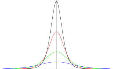
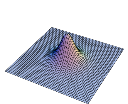
Figure 1: The first picture gives the cross section profiles of the regularized delta function defined in (17) for various values of $r\,$. The second picture gives a three dimensional impression of its shape.

Clearly both spin connection and curvature are regular functions of the coordinates for any non–zero value of the resolution parameter $r>0\,$. For any non–zero $x$ the curvature tends to zero in the blow down limit $r\rightarrow 0\,$. For $x=0$ the space is non–singular; the singular point of the orbifold $\mathbb{C}^{n}/\mathbb{Z}_{n}$ is replaced by a $\mathbb{CP}^{n-1}$ at $x=0\,$. Similarly, for fixed $r>0\,$, the resolution becomes flat far away from the blown up singularity $x\rightarrow\infty\,$. Contrary, if $r=0\,$, we see that parts of the spin connection and the whole curvature explode in the limit in which $x$ tends to zero. This shows that we can interpret the resolution as a regularization of the orbifold fixed point delta function. To make this more precise, consider the two dimensional complex case ($n=2$) for example, and compute $\text{tr}\,{\cal R}^{2}\,$. From (B.4) and (B.6) of appendix B we conclude that we can define a regularized orbifold delta function as

$$\delta_{r}(z,x)~{}=~{}\frac{1}{(n+1)(2\pi)^{2}}\,\text{tr}\,{\cal R}^{2}~{}=~{}-\frac{1}{2\pi^{2}}\frac{r^{2}}{(r+X)^{3}}{\bar{e}}e\,{\bar{\epsilon}}\epsilon~{},\qquad\int_{{\cal M}^{2}}\delta_{r}(z,x)~{}=~{}1~{}.$$ (17)

In figure 1 we have made schematic two and three dimensional pictures of this smeared out delta function in two complex dimensions.

3 Gauge Bundles on the Resolution

Next we turn to the construction of non–trivial gauge backgrounds on the resolution of the orbifold $\mathbb{C}^{n}/\mathbb{Z}_{n}\,$. For simplicity we consider only the gauge group $\mathrm{SO(32)}\,$. (The extension to the $\mathrm{E_{8}}\times\mathrm{E_{8}}^{\prime}$ gauge group is straightforward, and will be used at the end of section 4 to classify $\mathrm{E_{8}}\times\mathrm{E_{8}}^{\prime}$ models on the blowup.) We begin with a short review of gauge theories on orbifolds.

The group $\mathrm{SO(32)}$ is generated by 16 Cartan algebra elements $H_{I}\,$, with $I=1,\ldots 16$, and the elements $E_{w}$ parameterized by the vectorial weights $w=({\underline{\pm 1^{2},0^{16}}})\,$, with all permutations as the underline is denoting. These weights are the eigenvalues of the commutators

$$[H_{I},E_{w}]~{}=~{}w_{I}\,E_{w}~{}.$$ (18)

The gauge field 1–form $i\mathfrak{A}$ takes values in the algebra of $\mathrm{SO(32)}\,$; by $i\mathfrak{F}$ we denote its field strength. Gauge fields $i\mathfrak{A}$ on orbifolds can satisfy non–trivial boundary conditions

$$\mathfrak{A}(\Theta\,{\tilde{Z}})~{}=~{}U\,\mathfrak{A}({\tilde{Z}})\,U^{-1}~{},\qquad U~{}=~{}e^{2\pi i\,V^{I}H_{I}/n}~{},$$ (19)

for the orbifold action defined in (1). In order that this defines a proper $\mathbb{Z}_{n}$ action on vectorial weights, the shift vector $V$ can only contain either integer or only half–integer entries. (We use a normalization of the gauge shift vector $V$ without an explicit $\mathbb{Z}_{n}$ orbifold factor $1/n\,$.) The former are called vectorial shifts, and the latter spinorial shifts. In terms of the coordinates $x=|x|\,e^{i\varphi}$ and $z$, the orbifold action (19) takes the form of a periodicity condition for the angular variable $\varphi$

$$\mathfrak{A}(z,|x|,\varphi+2\pi)~{}=~{}U\,\mathfrak{A}(z,|x|,\varphi)\,U^{-1}~{}.$$ (20)

By a gauge transformation $g=e^{-i\,\varphi\,V^{I}H_{I}/n}$ this periodicity condition, can be rewritten as

$$i\mathfrak{A}_{g}~{}=~{}g(i\mathfrak{A}+\mathrm{d})g^{-1}~{}=~{}iA+i{\cal A}~{},\qquad i{\cal A}~{}=~{}i\,\frac{1}{n}\,V^{I}H_{I}\,\mathrm{d}\varphi~{},$$ (21)

where $iA$ is a periodic 1–form gauge potential, and $i{\cal A}$ is a constant Wilson–line background gauge connection. A gauge invariant way of stating that there is a Wilson–line is given by the following prescription: Consider a loop $\partial C=\{\varphi~{}~{}|~{}~{}0<\varphi<2\pi\}$ at fixed $z$ and $|x|\,$, and let $C$ represent any surface that has $\partial C$ as it boundary. By Stoke’s theorem we have

$$\int_{C}i{\cal F}~{}=~{}\int_{\partial C}i{\cal A}~{}=~{}2\pi\,i\,\frac{1}{n}\,V^{I}H_{I}~{},$$ (22)

where $i{\cal F}$ is the field strength of the $\mathrm{U(1)}$ background $i{\cal A}\,$. This completes the review of the description of gauge bundles on orbifolds.

We would like to find gauge backgrounds on the resolution of the orbifold $\mathbb{C}^{n}/\mathbb{Z}_{n}\,$. In order to preserve $N=1$ supersymmetry, the field strength $i{\cal F}$ of the background gauge potential $i{\cal A}$ has to satisfy the so–called Hermitian Yang–Mills equations

$${\cal F}_{AB}~{}=~{}0~{},\qquad{\cal F}_{{\underline{A}}\,{\underline{B}}}~{}=~{}0,\qquad\mbox{Tr}[{\cal F}]~{}\equiv~{}G^{A{\underline{A}}}\,{\cal F}_{{\underline{A}}A}~{}=~{}0~{},$$ (23)

see [1]. We study solutions of these equations on ${\cal M}^{n}$ for general $n$ in this section. These solutions should be regular over the whole manifold ${\cal M}^{n}$ as long as we have not yet taken the orbifold limit.

As in the previous section, all forms on ${\cal M}^{n}$ can be expressed in terms of the holomorphic 1–forms $e,\epsilon$ and their conjugates. Therefore we would like to reformulate these conditions in terms of these forms: The first two conditions of (23) simply mean that the field strength $i{\cal F}$ only contains mixed 2–forms, like $e{\bar{e}}\,$, ${\bar{\epsilon}}e$ and ${\bar{\epsilon}}\epsilon\,$. Taking the last equation in (23) as the definition of the trace of mixed 2–forms, we find

$$\mbox{Tr}[e{\bar{e}}]~{}=~{}\frac{1}{nM}\,\text{\small 1}\text{1}_{n-1}~{},\quad\mbox{Tr}[{\bar{e}}e]~{}=~{}-\frac{n\!-\!1}{nM}~{},\quad\mbox{Tr}[\epsilon{\bar{\epsilon}}]~{}=~{}\frac{1}{M^{\prime}}~{},\quad\mbox{Tr}[{\bar{\epsilon}}e]~{}=~{}\mbox{Tr}[{\bar{e}}\epsilon]~{}=~{}0~{},$$ (24)

in terms of the function $M(X)$ given in (9). Hence we are looking for gauge backgrounds which have field strengths that only contain mixed 2–forms that trace to zero, using the trace defined by (24).

In the following we give a few examples of explicit solutions of the Hermitean Yang–Mills equations on the resolution ${\cal M}^{n}\,$. We determine the corresponding gauge shift vector $V$ on the orbifold by computing the integral (22) in the blow down limit. We do not aim to give a complete classification here, but just construct a number of interesting examples to be considered later.

3.1 Standard Embedding: An $\boldsymbol{\mathrm{SU(n)}}$ Bundle

The first example is the well–known standard embedding of the spin–connection in the gauge bundle: $i{\cal A}_{\rm SE}=\Omega$, which is given in (14). This is indeed a solution of the Hermitean Yang–Mills equations as we can see from the field strength $i{\cal F}_{\rm SE}={\cal R}\,$: From the expression for ${\cal R}$, see eq. (15), it follows that it only contains mixed 2–forms, and by a direct computation we find

$$\mbox{Tr}[{\cal R}]~{}=~{}0~{}.$$ (25)

For any arbitrary value of the resolution parameter $r$ this gauge bundle fills a full $\mathrm{SU(n)}\subset\mathrm{SO(32)}\,$. To determine whether the standard embedding corresponds to an orbifold Wilson line, we compute the integral defined in (22):

$$\int_{\partial C}\Omega~{}=~{}\frac{2\pi i}{n}\,\frac{X}{r+X}\,\begin{pmatrix}\text{\small 1}\text{1}_{n-1}&0\\ 0&1\!-\!n\end{pmatrix}~{}\rightarrow~{}\frac{2\pi i}{n}\,\begin{pmatrix}\text{\small 1}\text{1}_{n-1}&0\\ 0&1\!-\!n\end{pmatrix}~{}.$$ (26)

This expression is diagonal, which shows that in the blow down limit ($r\rightarrow 0$) the standard embedding gives rise to the orbifold boundary conditions specified by the shift vector $V=(1^{n-1},1\!-\!n,0^{16-n})\,$. Notice that this also gives the geometrical shift vector (1) back.

3.2 Construction of $\boldsymbol{\mathrm{U(1)}}$ Background Gauge Field

Next we would like to construct a $\mathrm{U(1)}$ gauge background on the blowup of the orbifold $\mathbb{C}^{n}/\mathbb{Z}_{n}\,$. A first guess for such a background is the $\mathrm{U(1)}$ connection $i{\cal B}$ defined in (12), but this choice does not satisfy the last condition in (23) required to preserve supersymmetry. In order to obtain a background that does satisfy this requirement, we extend the connection as follows

$$i\,{\cal A}~{}=~{}i\,{\cal B}~{}+~{}e^{-\frac{p}{2}}(\bar{\partial}-\partial)e^{\frac{p}{2}}~{}=~{}i\,{\cal B}+\frac{1}{2}\,p^{\prime}(X)\,({\bar{\epsilon}}y-{\bar{y}}\epsilon)~{},$$ (27)

where $p(X)$ is an arbitrary function of the $\mathrm{SU(n)}$ isometry invariant variable $X\,$. As can be seen from the final expression, only its first derivative $p^{\prime}(X)$ is of physical relevance. The field strength 2–form is given by

$$i\,{\cal F}~{}=~{}(1-n\,p^{\prime}X){\bar{e}}\,e-(p^{\prime}X)^{\prime}\,{\bar{\epsilon}}\,\epsilon~{}.$$ (28)

By computing the trace of this gauge background, we obtain

$$\mbox{Tr}[i{\cal F}]~{}=~{}\frac{\big{(}p^{\prime}XM^{n-1}\big{)}^{\prime}}{M^{n-1}M^{\prime}}~{}-~{}\frac{n-1}{nM}~{}.$$ (29)

This background is supersymmetric if this trace vanishes, hence we obtain a simple differential equation for $p^{\prime}\,$. By solving this equation, and demanding that the solution is nowhere singular on the resolution ${\cal M}^{n}\,$, we determine the $\mathrm{U(1)}$ gauge connection

$$i{\cal A}~{}=~{}i{\cal B}~{}+~{}\frac{1}{2n}\frac{1}{X}\Big{[}1~{}-~{}\Big{(}\frac{r}{r+X}\Big{)}^{1-\frac{1}{n}}\Big{]}\big{(}{\bar{\epsilon}}y-{\bar{y}}\epsilon\big{)}~{},$$ (30)

with field strength

$$i{\cal F}~{}=~{}\Big{(}\frac{r}{r+X}\Big{)}^{1-\frac{1}{n}}\Big{(}{\bar{e}}e~{}-~{}\frac{n-1}{n^{2}}\,\frac{1}{r+X}\,{\bar{\epsilon}}\epsilon\Big{)}~{},$$ (31)

uniquely. Observe that $i{\cal A}$ and $i{\cal F}$ are indeed regular in the limit $x\rightarrow 0$ for finite values of the resolution parameter $r\,$. At $x=0$ the field strength diverges in the limit $r\rightarrow 0\,$. Hence, like the curvature (15), it can be used to define a regularized orbifold fixed point delta function, similar to the one depicted in figure 1.

Using this background, we can easily construct a large class of $\mathrm{U(1)}$ bundles. In $\mathrm{SO(32)}$ we can embed at most 16 mutually commuting $\mathrm{U(1)}$s, precisely parameterizing a Cartan subgroup. Using the generators $H_{I}$ of this Cartan subgroup, we define

$$i{\cal A}_{V}~{}=~{}i{\cal A}\,V^{I}H_{I}~{},\qquad i{\cal F}_{V}~{}=~{}i\,{\cal F}\,V^{I}H_{I}~{},$$ (32)

where $i{\cal A}$ and $i{\cal F}$ are given in (30) and (31), respectively. This bundle is well–defined only if the first Chern class is integral on all closed 2–cycles for all relevant representations. By a direct computation we find for the integral over the $\mathbb{CP}^{1}$ at $x=0$

$$\frac{1}{~{}2\pi i}\int_{\mathbb{CP}^{1}}i{\cal F}_{V}~{}=~{}V^{I}H_{I}~{},$$ (33)

using (B.2) of appendix B. Therefore, as in the orbifold case (see below (19)) the entries of $V$ are either all integer or all half integer. The same condition is obtained, because the gauge background corresponds to orbifold boundary conditions in the blow down limit: By computing the integral (22) we find

$$\int_{\partial C}i{\cal A}_{V}~{}=~{}-\frac{2\pi i}{n}\,V^{I}H_{I}\,\Big{[}1~{}-~{}\Big{(}\frac{r}{r+X}\Big{)}^{1-\frac{1}{n}}\Big{]}~{}\rightarrow~{}-\frac{2\pi i}{n}\,V^{I}H_{I}~{},$$ (34)

in the blow down limit $r\rightarrow 0\,$. This means that the $\mathrm{U(1)}$ bundles on the non–compact Calabi–Yau ${\cal M}^{n}$ are quantized in units of $1/n\,$.

3.3 An $\boldsymbol{\mathrm{SU(n\!-\!1)}}$ Bundle

The final bundle we describe has an $\mathrm{SU(n\!-\!1)}$ structure. In (12) we obtained a $\mathrm{U(n\!-\!1)}$ and a $\mathrm{U(1)}$ bundle on $\mathbb{CP}^{n-1}\,$. By combining them we can obtain an $\mathrm{SU(n\!-\!1)}$ gauge connection and field strength

$$i\tilde{\cal A}~{}=~{}i\tilde{\cal B}~{}+~{}\frac{1}{n-1}\,i{\cal B}~{},\qquad i\tilde{\cal F}~{}=~{}\mathrm{d}(i\tilde{\cal A})~{}+~{}(i\tilde{\cal A})^{2}~{}=~{}e\,{\bar{e}}~{}+~{}\frac{1}{n-1}\,{\bar{e}}\,e~{}.$$ (35)

It is not difficult to check that $\tilde{\cal A}$ is indeed an $\mathrm{SU(n\!-\!1)}$ gauge potential, i.e. $\text{tr}\,i\tilde{\cal A}=\text{tr}\,i\tilde{\cal F}=0\,$ (trace over the external $\mathrm{SU(n\!-\!1)}$ indices). The field strength is nowhere vanishing. In addition using the trace of mixed 2–forms defined in (24), we infer that this defines a supersymmetric background on ${\cal M}^{n}\,$, because $\mbox{Tr}[i\tilde{\cal F}]=0\,$. However, the integral over $\partial C$ is zero, because it does not contain any $\epsilon$ or ${\bar{\epsilon}}$ forms. Hence, this configuration does not correspond to a Wilson line configuration in the orbifold limit, and cannot be described by a gauge shift vector on the orbifold $\mathbb{C}^{n}/\mathbb{Z}_{n}\,$. Thus this gauge bundle is not directly visible from the orbifold point of view.

4 Consistent Compactifications of Super Yang–Mills theory coupled to Supergravity

In the previous section we have constructed some gauge backgrounds on the blowup ${\cal M}^{n}$ of the orbifold $\mathbb{C}^{n}/\mathbb{Z}_{n}\,$. We have required that they satisfy the Hermitean Yang–Mills equations on the resolution. When these conditions are fulfilled, the background preserves $N=1$ supersymmetry in six or four dimensions, depending on whether $n=2$ or $n=3\,$, respectively. In the following we will keep $n$ generic, but have applications for these cases in mind. When the supersymmetric gauge theory is coupled to supergravity, we encounter one further (topological) consistency requirement. This condition results from the Bianchi identity of the 2–form $B$ of the supergravity multiplet,

$$\mathrm{d}{\cal H}~{}=~{}\text{tr}{\cal R}^{2}~{}-~{}\text{tr}(i{\cal F})^{2}~{},$$ (36)

where ${\cal H}$ is its 3–form field strength. Both the trace over the curvature 2–form ${\cal R}\in\mathrm{SU(n)}$ and the $\mathrm{U(16)}\subset\mathrm{SO(32)}$ gauge background $i{\cal F}$ are performed in fundamental representations of $\mathrm{SU(n)}\,$, so no relative normalization factor is required. By Stoke’s theorem the integrated Bianchi identity over a closed 4–cycle $C^{4}$ vanishes [47]:

$$0~{}=~{}\int_{C^{4}}\Big{\{}\text{tr}{\cal R}^{2}~{}-~{}\text{tr}(i{\cal F})^{2}\Big{\}}~{}.$$ (37)

To investigate the consequences of the integrated Bianchi identity for the blowup ${\cal M}^{n}$ of the orbifold $\mathbb{C}^{n}/\mathbb{Z}_{n}\,$, we need to determine the 4–cycles of ${\cal M}^{n}\,$.

To describe the compact and non–compact cycles of the resolution manifold ${\cal M}^{n}\,$, it is important to remember that this space was constructed as a cone over $\mathbb{CP}^{n-1}\,$. Hence, many cycles of ${\cal M}^{n}$ are inherited from $\mathbb{CP}^{n-1}\,$, therefore we describe the relevant cycles of this base space first: Obviously, $\mathbb{CP}^{k}$ is a $2k$–cycle itself, in particular, $\mathbb{CP}^{1}$ is a 2–cycle and $\mathbb{CP}^{2}$ is a 4–cycle. Moreover, for any group $G$ with $\pi_{1}(G)=1$, we have $\pi_{2}(G/H)=\pi_{1}(H)$ for a proper subgroup $H\subset G\,$. Because $\mathbb{CP}^{n-1}=\mathrm{SU(n)}/\mathrm{U(n\!-\!1)}\,$, this implies that $\pi_{2}(\mathbb{CP}^{n-1})=\pi_{1}(\mathrm{U(1)})=\mathbb{Z}\,$. Since the homology groups can be thought of as the Abelian part of the fundamental groups, we conclude that $H_{2}(\mathbb{CP}^{n-1})=\mathbb{Z}\,$. This means that $\mathbb{CP}^{n-1}$ has a non–contractible 2–cycle, which can be represented as the embedding of $\mathbb{CP}^{1}$ into $\mathbb{CP}^{n-1}$. Using these cycles of $\mathbb{CP}^{n-1}$ we can describe the 4–cycles of the resolutions ${\cal M}^{2}$ and ${\cal M}^{3}\,$. The manifold ${\cal M}^{2}$ is four dimensional hence it is its own non–compact 4–cycle. The resolution ${\cal M}^{3}$ (and all other ${\cal M}^{n}\,$, $n>2\,$) has two 4–cycles: At the point $x=0$ the resolution ${\cal M}^{3}$ looks like a $\mathbb{CP}^{2}\,$, hence $\mathbb{CP}^{2}$ is a compact 4–cycle of ${\cal M}^{3}\,$. In addition, the space ${\cal M}^{3}$ contains a real four dimensional manifold ${\cal M}^{2}\,$, which defines a second non–compact cycle of ${\cal M}^{3}\,$. Below we discuss the resulting consequences of integrated Bianchi identities in six and four dimensional models.

4.1 Consistent resolution of $\boldsymbol{\mathbb{C}^{2}/\mathbb{Z}_{2}}$ models

The Bianchi identity integrated over the resolution ${\cal M}^{2}$ becomes

$$\int_{\partial{\cal M}^{2}}{\cal H}~{}=~{}\int_{{\cal M}^{2}}\Big{\{}\text{tr}{\cal R}^{2}~{}-~{}\text{tr}(i{\cal F})^{2}\Big{\}}~{},$$ (38)

where the boundary $\partial{\cal M}^{2}$ at $x\rightarrow\infty$ has the topology of $\mathbb{CP}^{1}\times S^{1}\,$. If the 3–form ${\cal H}$ is trivial at $x\rightarrow\infty$, this condition reduces to the compact case, and this integral vanishes. Making this simplifying assumption, we see that the standard embedding is of course a solution, because the Bianchi identity is satisfied locally. The $\mathrm{SU(n\!-\!1)}$ bundle (35) does not exist on ${\cal M}^{2}\,$, with $n=2\,$. For the $\mathrm{U(1)}$ bundles (32) the vanishing integrated Bianchi identity implies that

$$V^{2}~{}-~{}6~{}=~{}0~{}.$$ (39)

The relevant integrals (B.6) and (B.9) are evaluated in appendix B. This condition is similar to the relation for fractional instantons given in [48, 49]. The solutions to the integrated Bianchi conditions and the resulting gauge groups are given in table 1.

Model	$G_{\rm blowup}$	Representations of Hypers
St. Emb.	$\mathrm{SO(28)}\times\mathrm{SU(2)}$	$\frac{5}{8}(\mathbf{28},\mathbf{2})+\frac{45}{16}(\mathbf{1},\mathbf{1})$
$(0^{13},1^{2},2)$	$\mathrm{SO(26)}\times\mathrm{U(2)}\times\mathrm{U(1)}$	$\frac{1}{8}(\mathbf{26},\mathbf{2})_{1}+\frac{1}{8}(\mathbf{1},\mathbf{2})_{1}+\frac{7}{8}(\mathbf{1},\mathbf{1})_{2}+\frac{7}{8}(\mathbf{26},\mathbf{1})_{2}+\frac{17}{8}(\mathbf{1},\mathbf{2})_{3}$
$(0^{10},1^{6})$	$\mathrm{SO(20)}\times\mathrm{U(6)}$	$\frac{1}{8}(\mathbf{20},\mathbf{6})_{1}+\frac{7}{8}(\mathbf{1},\mathbf{15})_{2}$
$({\frac{1}{2}}^{15},{\,\mbox{-}}\frac{3}{2})$	$\mathrm{U(15)}\times\mathrm{U(1)}$	$\frac{1}{8}(\mathbf{15})_{1}+\frac{1}{8}(\mathbf{105})_{1}+\frac{7}{8}(\mathbf{15})_{2}$

Table 1: The spectra of the standard embedding and the three $\mathrm{U(1)}$ gauge bundle models on the resolution of the orbifold $\mathbb{C}^{2}/\mathbb{Z}_{2}$ with vanishing ${\cal H}$ are displayed. The $\mathrm{U(1)}$ charges are the eigenvalues of $H_{V}\,$, and determine the multiplicities via (43).

To obtain the spectra of the models as given in table 1 we start from the anomaly polynomial $I_{12}$ of the Majorana–Weyl gaugino in ten dimensions [47, 50]

$$I_{12}~{}=~{}\frac{1}{2}\,\frac{1}{(2\pi)^{5}}\Big{[}-\frac{1}{720}\text{tr}(i\mathfrak{F})^{6}~{}+~{}\frac{1}{24\cdot 48}\text{tr}(i\mathfrak{F})^{4}\text{tr}\,\mathfrak{R}^{2}~{}-~{}\frac{1}{256}\text{tr}(i\mathfrak{F})^{2}\Big{(}\frac{1}{45}\text{tr}\,\mathfrak{R}^{4}+\frac{1}{36}(\text{tr}\,\mathfrak{R}^{2})^{2}\Big{)}$$

$$~{}+~{}\frac{496}{64}\Big{(}\frac{1}{2\cdot 2835}\text{tr}\,\mathfrak{R}^{6}+\frac{1}{4\cdot 1080}\text{tr}\,\mathfrak{R}^{2}\text{tr}\,\mathfrak{R}^{4}+\frac{1}{8\cdot 1296}(\text{tr}\,\mathfrak{R}^{2})^{3}\Big{)}\Big{]}~{}.$$ (40)

We then expand $\mathfrak{R}={\cal R}+R$ and $i\mathfrak{F}=i{\cal F}+iF$ around the background set by the curvature ${\cal R}$ of the blowup ${\cal M}^{2}$ and the field strength $i{\cal F}$ of the gauge bundle of the corresponding model; $R$ and $iF$ denote the curvature and gauge field strength in six dimensions. This gives an expression for the anomaly polynomial

$$2(2\pi)^{5}\,I_{12}~{}=~{}-\frac{1}{256}\Big{[}(i{\cal F})^{2}\,\text{tr}\big{[}H_{V}^{2}\big{]}-\frac{496}{12}\text{tr}\,{\cal R}^{2}\Big{]}\Big{(}\frac{1}{45}\text{tr}\,R^{4}+\frac{1}{36}(\text{tr}\,R^{2})^{2}\Big{)}$$ (41)

$$-\frac{1}{48}\Big{[}(i{\cal F})^{2}\,\text{tr}\big{[}H_{V}^{2}(iF)^{4}\big{]}-\frac{1}{12}\text{tr}\,{\cal R}^{2}\,\text{tr}(iF)^{4}\Big{]}~{}+~{}\frac{1}{192}\Big{[}(i{\cal F})^{2}\,\text{tr}\big{[}H_{V}^{2}(iF)^{2}\big{]}-\frac{1}{12}\text{tr}\,{\cal R}^{2}\,\text{tr}(iF)^{2}\Big{]}\text{tr}\,R^{2}~{},$$

where $H_{V}=V^{I}H_{I}\,$. Integrating this expression over ${\cal M}^{2}\,$, using (B.6) and (B.9) again, and some group theoretical trace identities, the six dimensional anomaly polynomial can be cast into the form

$$(2\pi)^{3}I_{8}~{}=~{}-\frac{1}{24}\text{tr}\big{[}{\scriptstyle\frac{1}{2}}N_{V}\,(iF)^{4}\big{]}+\frac{1}{96}\text{tr}\big{[}{\scriptstyle\frac{1}{2}}N_{V}\,(iF)^{2}\big{]}\,\text{tr}\,R^{2}-\frac{\text{tr}[{\scriptstyle\frac{1}{2}}N_{V}]}{128}\Big{(}\frac{1}{45}\text{tr}\,R^{4}+\frac{1}{36}(\text{tr}\,R^{2})^{2}\Big{)}~{}.$$ (42)

The operator

$$N_{V}~{}=~{}\frac{1}{4}\Big{(}H_{V}^{2}-\frac{1}{2}\Big{)}$$ (43)

counts the number of matter hyper multiplets in various representations of the unbroken subgroup of $\mathrm{SO(32)}\,$. The trace tr in this expression is taken over the full adjoint of $\mathrm{SO(32)}\,$. It has to be decomposed into irreducible representations of the unbroken gauge group. On each irreducible representation the operator $H_{V}$ and therefore $N_{V}$ have definite eigenvalues. In particular on the adjoint of the unbroken group we find $N_{V}=-1/8\,,$ while on all other representations $N_{V}$ is positive, see table 1. This reflects the fact that the chiralities of the gauginos and the matter hyperinos is opposite.

Also the values of the multiplicity factors in table 1 can be understood easily by comparing these numbers with the spectra one expects on the compact orbifold $T^{4}/\mathbb{Z}_{2}\,$: The bulk states give an 1/16 of the anomaly at each of the 16 fixed points of $T^{4}/\mathbb{Z}_{2}\,$. Because all the charged bulk states come from the gauge field and the gaugino, which form doublets under the $\mathrm{SU(2)}$ holonomy group, we get their contributions two times, hence we obtain a factor $1/8\,$. In this table we also encounter the factor $17/8$, which means that the states both arise as fixed point states (four of them at a given fixed point) and a single bulk state. Finally, the factor $7/8$ arises from two fixed point states. These states are precisely those needed to supply the opposite chirality of the gaugino states that correspond to the symmetry breaking of $\mathrm{SO(28)}\times\mathrm{SU(2)}\times\mathrm{SU(2)}$ to the gauge group of the corresponding model. Again because of $\mathrm{SU(2)}$ holonomy, this means that $1/8$ of the fixed states disappears via the Higgs mechanism to form massive vector multiplets, leaving a multiplicity factor $7/8\,$.

The procedure of integrating the anomaly polynomial coincides with computing the Dirac indices on the resolution ${\cal M}^{2}$ using Atiyah–Singer theorems. We have confirmed that the irreducible gauge anomalies cancel using techniques explained in [51, 52].

4.2 Consistent resolution of $\boldsymbol{\mathbb{C}^{3}/\mathbb{Z}_{3}}$ models

Model	$G_{\rm blowup}$	Representations
St. Emb.	$\mathrm{SO(26)}\times\mathrm{U(1)}$	$\frac{12}{9}(\mathbf{26})_{1}+\frac{12}{9}(\mathbf{1})_{-2}$
$(0^{12},1^{3},3)$	$\mathrm{SO(24)}\times\mathrm{U(3)}\times\mathrm{U(1)}$	$\frac{1}{9}(\mathbf{24},\mathbf{3})_{1}+\frac{2}{9}(\mathbf{1},\mathbf{3})_{{\,\mbox{-}}2}+(\mathbf{24},\mathbf{1})_{{\,\mbox{-}}3}+\frac{26}{9}(\mathbf{1},\overline{\mathbf{3}})_{{\,\mbox{-}}4}$
$(0^{13},2^{3})$	$\mathrm{SO(26)}\times\mathrm{U(3)}$	$\frac{1}{9}(\mathbf{26},\overline{\mathbf{3}})_{{\,\mbox{-}}2}+\frac{26}{9}(\mathbf{1},\mathbf{3})_{{\,\mbox{-}}4}$
$(0^{10},1^{4},2^{2})$	$\mathrm{SO(20)}\times\mathrm{U(4)}\times\mathrm{U(2)}$	$\frac{1}{9}(\mathbf{1},\overline{\mathbf{4}},\mathbf{2})_{1}+\frac{1}{9}(\mathbf{20},\mathbf{4},\mathbf{1})_{1}+\frac{1}{9}(\mathbf{1},\overline{\mathbf{6}},\mathbf{1})_{{\,\mbox{-}}2}$
		$+\frac{1}{9}(\mathbf{20},\mathbf{1},\overline{\mathbf{2}})_{{\,\mbox{-}}2}+(\mathbf{1},\overline{\mathbf{4}},\overline{\mathbf{2}})_{{\,\mbox{-}}3}+\frac{26}{9}(\mathbf{1},\mathbf{1},\mathbf{1})_{{\,\mbox{-}}4}$
$(0^{7},1^{8},2)$	$\mathrm{SO(14)}\times\mathrm{U(8)}\times\mathrm{U(1)}$	$\frac{1}{9}(\mathbf{1},\overline{\mathbf{8}})_{1}+\frac{1}{9}(\mathbf{14},\mathbf{8})_{1}+\frac{1}{9}(\mathbf{1},\overline{\mathbf{28}})_{{\,\mbox{-}}2}+\frac{1}{9}(\mathbf{14},\mathbf{1})_{{\,\mbox{-}}2}+(\mathbf{1},\overline{\mathbf{8}})_{{\,\mbox{-}}3}$
$(0^{4},1^{12})$	$\mathrm{SO(8)}\times\mathrm{U(12)}$	$\frac{1}{9}(\mathbf{8},\mathbf{12})_{1}+\frac{1}{9}(\mathbf{1},\overline{\mathbf{66}})_{{\,\mbox{-}}2}$
$({\frac{1}{2}}^{14},\frac{3}{2},{\,\mbox{-}}\frac{5}{2})$	$U(14)\times U(1)\times U(1)$	$\frac{1}{9}(\overline{\mathbf{14}})_{1}+\frac{1}{9}(\mathbf{1})_{1}+\frac{1}{9}(\mathbf{91})_{1}+\frac{1}{9}(\mathbf{14})_{{\,\mbox{-}}2}$
		$+\frac{1}{9}(\overline{\mathbf{14}})_{{\,\mbox{-}}2}+(\overline{\mathbf{14}})_{{\,\mbox{-}}3}+\frac{26}{9}(\mathbf{1})_{{\,\mbox{-}}4}$
$({\frac{1}{2}}^{12},{\frac{3}{2}}^{4})$	$\mathrm{U(4)}\times\mathrm{U(12)}$	$\frac{1}{9}(\mathbf{4},\overline{\mathbf{12}})_{1}+\frac{1}{9}(\mathbf{1},\mathbf{66})_{1}+\frac{1}{9}(\overline{\mathbf{4}},\overline{\mathbf{12}})_{{\,\mbox{-}}2}+(\overline{\mathbf{6}},\mathbf{1})_{{\,\mbox{-}}3}$

Table 2: This table gives the spectra of the standard embedding and the seven $\mathrm{U(1)}$ gauge bundle models on the resolution of the orbifold $\mathbb{C}^{3}/\mathbb{Z}_{3}$ with vanishing ${\cal H}$. The charges are the eigenvalues of the operator $H_{V}$, and determine the multiplicities according to (50).

On the blowup ${\cal M}^{3}$ of the orbifold $\mathbb{C}^{3}/\mathbb{Z}_{3}$ the Bianchi identity gives rise to two conditions, because there are two independent 4–cycles: $\mathbb{CP}^{2}$ at the singularity and ${\cal M}^{2}\,$. As we discussed above, the Bianchi identity integrated over ${\cal M}^{2}$ can in principle have a non–vanishing boundary integral over ${\cal H}\,$, but this boundary contribution vanishes, if we assume that the background for ${\cal H}$ is trivial. Under this assumption we have in principle two independent consistency requirements from (37):

$$\int_{\mathbb{CP}^{2}}\Big{\{}\text{tr}{\cal R}^{2}~{}-~{}\text{tr}(i{\cal F})^{2}\Big{\}}~{}=~{}0~{},\qquad\int_{{\cal M}^{2}}\Big{\{}\text{tr}{\cal R}^{2}~{}-~{}\text{tr}(i{\cal F})^{2}\Big{\}}~{}=~{}0~{}.$$ (44)

Here ${\cal M}^{2}$ denotes the space ${\cal M}^{3}$ with, say $z^{1}=0\,$. The easiest solution of these conditions is of course again the standard embedding.

We describe the solutions of these two consistency conditions for the $U(1)$ gauge backgrounds (32). First of all, we find that the two conditions are equivalent. Indeed, the first condition gives

$$-48\pi^{2}~{}=~{}\int_{\mathbb{CP}^{2}}\text{tr}{\cal R}^{2}~{}=~{}\int_{\mathbb{CP}^{2}}\text{tr}(i{\cal F}_{V})^{2}~{}=~{}-4\pi^{2}\,V^{2}~{},$$ (45)

while the second reads

$$16\pi^{2}~{}=~{}\int_{{\cal M}^{2}}\text{tr}{\cal R}^{2}~{}=~{}\int_{{\cal M}^{2}}\text{tr}(i{\cal F}_{V})^{2}~{}=~{}\frac{4\pi^{2}}{3}\,V^{2}~{}.$$ (46)

To obtain these results we have used the integrals (B.6) and (B.9). Hence both conditions are equivalent, and imply that the vector $V$ has to satisfy

$$V^{2}~{}=~{}12~{}.$$ (47)

The solutions to this condition and the resulting gauge groups and spectra are collected in table 2 for the $\mathrm{SO(32)}$ theory.

To obtain the spectra of the models given in table 2, we again start from the anomaly polynomial (40) for the gaugino in ten dimensions. Because the result for the standard embedding are well–known, we only focus on the $U(1)$ gauge bundles here. We insert the background of the resolution manifold ${\cal M}^{3}$ and the gauge bundle of the corresponding model into this anomaly polynomial. Using the branching of the Lorentz and gauge group, and some additional group theoretical properties, the anomaly polynomial $I_{12}$ on the resolution ${\cal M}^{3}$ can be written as

$$2(2\pi)^{5}I_{12}~{}=~{}(i{\cal F})^{3}\Big{\{}-\frac{1}{36}\text{tr}[H_{V}^{3}(iF)^{3}]~{}+~{}\frac{1}{9\cdot 32}\text{tr}[H_{V}^{3}\,iF]\text{tr}\,R^{2}\Big{\}}$$

$$~{}+~{}2\,i{\cal F}\,\text{tr}\,{\cal R}^{2}\Big{\{}\frac{1}{9\cdot 32}\text{tr}[H_{V}(iF)^{3}]~{}-~{}\frac{1}{9\cdot 256}\text{tr}[H_{V}iF]\text{tr}\,R^{2}\Big{\}}~{}.$$ (48)

This expression is integrated over ${\cal M}^{3}$, using the expressions (B.10) and (B.12) of appendix B, to give

$$-i\,(2\pi)^{2}\,I_{6}~{}=~{}\frac{1}{6}\text{tr}\big{[}\frac{1}{2}\,N_{V}(iF)^{3}\big{]}~{}-~{}\frac{1}{48}\text{tr}\big{[}\frac{1}{2}\,N_{V}\,iF\big{]}\,\text{tr}\,R^{2}~{}.$$ (49)

This expression for the anomaly in four dimensions can be used to read off the chiral spectrum of the model. The operator

$$N_{V}~{}=~{}\frac{1}{6}\Big{(}-\frac{1}{3}H_{V}^{2}+1\Big{)}H_{V}$$ (50)

gives the multiplicity of the irreducible representations after decomposing the trace tr again. It has been normalized such that in (49) we take into account that from the adjoint of $\mathrm{SO(32)}$ all complex representations appear in conjugate pairs. The charges $H_{V}$, and therefore $N_{V}\,$, of such a pair are opposite, so for the four dimensional anomaly they contribute twice.

$k$	Shift Vector	$G_{\rm blowup}$	$G_{\rm blow\ down}$
$2$	$(0^{12},1^{2},2,3)$	$\mathrm{SO(20)}\times\mathrm{U(2)}\times\mathrm{U(1)}\times\mathrm{U(1)}$	$\mathrm{SO(26)}\times\mathrm{U(3)}$
	$(0^{9},1^{6},3)$	$\mathrm{SO(14)}\times\mathrm{U(6)}\times\mathrm{U(1)}$	$\mathrm{SO(20)}\times\mathrm{U(6)}$
	$(0^{10},1^{3},2^{3})$	$\mathrm{SO(16)}\times\mathrm{U(3)}\times\mathrm{U(3)}$
	$(0^{7},1^{7},2^{2})$	$\mathrm{SO(10)}\times\mathrm{U(7)}\times\mathrm{U(2)}$	$\mathrm{SO(14)}\times\mathrm{U(9)}$
	$(0^{4},1^{11},2)$	$\mathrm{SO(4)}\times\mathrm{U(11)}\times\mathrm{U(1)}$	$\mathrm{SO(8)}\times\mathrm{U(12)}$
$4$	$(0^{14},3^{2})$	$\mathrm{SO(20)}\times\mathrm{U(2)}$	$\mathrm{SO(32)}$
	$(0^{13},1^{2},4)$	$\mathrm{SO(18)}\times\mathrm{U(2)}\times\mathrm{U(1)}$	$\mathrm{SO(26)}\times\mathrm{U(3)}$
	$(0^{12},1,2^{2},3)$	$\mathrm{SO(16)}\times\mathrm{U(1)}\times\mathrm{U(2)}\times\mathrm{U(1)}$
	$(0^{9},1^{5},2,3)$	$\mathrm{SO(10)}\times\mathrm{U(5)}\times\mathrm{U(1)}\times\mathrm{U(1)}$	$\mathrm{SO(20)}\times\mathrm{U(6)}$
	$(0^{10},1^{2},2^{4})$	$\mathrm{SO(12)}\times\mathrm{U(2)}\times\mathrm{U(4)}$
$6$	$(0^{13},1,2,4)$	$\mathrm{SO(14)}\times\mathrm{U(1)}\times\mathrm{U(1)}\times\mathrm{U(1)}$	$\mathrm{SO(26)}\times\mathrm{U(3)}$

Table 3: The first column gives the number of times we have used the $\mathrm{SU(2)}$ bundle (35). The second column gives the vectorial shift vector $V$ of these $\mathrm{SU(2)}$–$\mathrm{U(1)}$ bundle models. The final two columns give the resulting gauge groups on the resolution and in the blow down limit.

In table 2 the charges $H_{V}$ and the multiplicity values $N_{V}$ are indicated. Most multiplicities are multiples of $1/9\,$. The reason for this is that we compute the spectrum on the resolution of the non–compact orbifold $\mathbb{C}^{3}/\mathbb{Z}_{3}\,$. As has been shown in [23] the anomaly of bulk fields at a fixed point is $1/27$ of the zero mode anomaly on $T^{6}/\mathbb{Z}_{3}\,$, but each bulk state has a multiplicity of three due to the $\mathrm{SU(3)}$ holonomy. Hence in total we find a factor of $1/9\,$. For states localized at the orbifold fixed point we do not have such fractional multiplicity factors. In table 2 these states can be spotted easily, either they have a multiplicity factor of $1\,$, or $26/9\,$. In the latter case $1/9$ of the fixed point state has paired up with a bulk state.

Using the shift vectors as given in table 2 it is straightforward to read off the gauge enhancement in the blow down limit. In table 4 the resulting gauge groups are displayed to facilitate the comparison in section 5.2 of our blowup models with the heterotic $\mathbb{Z}_{3}$ orbifold models in four dimensions. Here we only notice that all gauge groups except $\mathrm{SO(32)}$ of heterotic $\mathbb{Z}_{3}$ models are recovered in this limit. To see how this model could arise, we would like to make some comments on models in which the $\mathrm{U(1)}$ bundles (32) and multiple embeddings (say $k$ times) of the $\mathrm{SU(2)}$ gauge background (35) are combined. As long as we make sure that in this combined embedding all parts still commute with each other, we are guaranteed that the Hermitian Yang–Mills equations remain satisfied. In this case the integrated Bianchi conditions for $\mathbb{CP}^{2}$ and ${\cal M}^{2}$ give the conditions

$$-48\pi^{2}~{}=~{}k\,6\pi^{2}~{}-~{}4\pi^{2}\,V^{2}~{},\qquad\int_{\partial{\cal M}^{2}}{\cal H}~{}=~{}16\pi^{2}~{}-~{}\frac{4\pi^{2}}{3}\,V^{2}~{}=~{}-k\,2\pi^{2}~{},$$ (51)

respectively, which are not equivalent anymore. The second equation says that we can allow for multiple embeddings of $\mathrm{SU(2)}$ bundles, only if we have non–trivial ${\cal H}$ flux at infinity (i.e. at $\partial{\cal M}^{2}$). But then the geometrical background needs to have torsion and hence is non–Kähler [53, 54]. This means that the Ricci–flat Kähler manifold ${\cal M}^{3}\,$, discussed in this work, does not define the appropriate setting to investigate such gauge bundle configurations.

Even though the full explicit construction of models with such combined $\mathrm{SU(2)}$–$\mathrm{U(1)}$ bundles lies beyond the scope of this paper, let us make some speculations: Let us assume that the integrals in the required torsion background still lead to the first equation (51). This condition simply equates the instanton numbers on $\mathbb{CP}^{2}$ (upto a normalization factor), so one may expect that their values stay the same when one introduces torsion. We see that the model with $n=4$ and $V=(0^{14},3^{2})$ satisfies this condition. This model in blow down reproduces the $\mathrm{SO(32)}$ model, which we are not able to construct using the standard embedding or $\mathrm{U(1)}$ bundles alone. Using such combined $\mathrm{SU(2)}$–$\mathrm{U(1)}$ bundles, one can consider many other models that satisfy the consistency condition (51). The resulting solutions for the $\mathrm{SO(32)}$ theory and the gauge groups on the resolution and in the blow down limit are given in table 3. (A similar table can be produced for the $\mathrm{E_{8}}\times\mathrm{E_{8}}^{\prime}$ case but will not be given here.) The reason that in the blow down the rank of the gauge group is enhanced is because the $\mathrm{SU(2)}$ bundles disappear inside the orbifold singularity: they only have support on the $\mathbb{CP}^{2}\,$, that is on the blowup of the orbifold singularity. The blow down gauge groups are precisely all possible gauge groups for $\mathbb{Z}_{3}$ heterotic $\mathrm{SO(32)}$ orbifolds, except the $\mathrm{SO(2)}\times\mathrm{U(15)}$ model. Let us emphasize that our work does not strictly speaking prove that these models exist, but gives strong hints that they might.

5 Matching with Heterotic Orbifold Models

We now compare our results on the resolutions ${\cal M}^{n}$ of $\mathbb{C}^{n}/\mathbb{Z}_{n}\,$, for $n=2,3$, using field theory techniques only, with the heterotic string on such orbifolds. Before we turn to the details of this comparison, we first review the requirements on heterotic orbifolds, see e.g. [11, 12, 55, 56].

In the heterotic string a perturbative $\mathbb{C}^{n}/\mathbb{Z}_{n}$ or $T^{2n}/\mathbb{Z}_{n}$ orbifold is completely specified by the action of the orbifold operator on the spacetime geometry and on the gauge bundle. (We describe only the heterotic $\mathrm{SO(32)}$ string here, as the $\mathrm{SO(32)}$ gauge theory has mostly been focused on in this work; the extension to the $\mathrm{E_{8}}\times\mathrm{E_{8}}^{\prime}$ case is straightforward.) The geometric action is required to be well–defined on bosons and spinors, and leaves one spinor invariant to preserve some supersymmetry. The geometrical shift (1) already satisfies all these requirements in the field theoretical description as was discussed below that equation. The orbifold action on the gauge bundle is instead specified by the vector $V$, as explained in section 3. In addition to the demand that its entries, $V^{I}\,$, should either all be integer or all half-integer, we need to require that

$$\sum V^{I}~{}=~{}0~{}{\rm mod}~{}2~{}.$$ (52)

The reason for this is that the (massive) spectrum of the heterotic $\mathrm{SO(32)}$ string also contains positive chirality spinorial representations. This condition ensures that the $\mathbb{Z}_{n}$ orbifold action has also order $n$ on positive chiral spinors as well. We have enforced this constraint on all gauge shift vectors given in tables 1, 2 and 5 by including some appropriate minuses of some shift vector entries. For the field theory models, we have discussed, this constraint is irrelevant because the models and spectra are identical. Finally, we get to the only real string condition: Modular invariance of the partition function imposes the following relation

$$V^{2}~{}=~{}\phi^{2}~{}{\rm mod}~{}2n$$ (53)

among the geometrical and gauge shifts.

The various string conditions described here are reflected in the construction of the smooth resolutions of the orbifold singularity and its $\mathrm{U(1)}$ bundles: The requirement of preserving a certain amount of supersymmetry forced the resolution to be Calabi–Yau, i.e. a Ricci–flat Kähler manifold with $\mathrm{SU(n)}$ holonomy. In the blow down limit we read off a geometrical shift, see (26), which satisfies the above requirements. Similarly, integrality of the first Chern class (33) of the $\mathrm{U(1)}$ bundle on the blowup was linked to the orbifold conditions of the gauge shift $V$ via (34). The modular invariance condition (53) should be identified with the integrated Bianchi identity condition (38) on the resolution. The latter condition is much more restrictive, indeed, all the gauge shifts listed in tables 1, 2 and 5 satisfy the corresponding modular invariance condition (53) of $\mathbb{C}^{2}/\mathbb{Z}_{2}$ and $\mathbb{C}^{3}\mathbb{Z}_{3}$ orbifold, respectively.

The conditions described here apply both to the non–compact orbifolds $\mathbb{C}^{n}/\mathbb{Z}_{n}$ and to their compact relatives $T^{2n}/\mathbb{Z}_{n}\,$. The compact orbifolds can be equipped with discrete Wilson lines, which need to fulfill additional consistency conditions [55, 56]. These extra requirements are equivalent to local modular invariance conditions (53) at each of the fixed points, for the local gauge shift vectors of those fixed points, as has been demonstrated in [23]. The reason for these local conditions can also be understood from the blowup perspective: We expect, that patching of various copies of the resolution geometry with gauge bundles only gives mild modifications in the vicinity of the gluing areas, leading to a satisfactory description of the whole compact orbifold. Then the effect of discrete Wilson lines, i.e. different local gauge shifts, corresponds to a space constructed by gluing patches with the same base geometry ${\cal M}^{n}$ but different $\mathrm{U(1)}$ bundles. Since each ${\cal M}^{3}$ contains a $\mathbb{CP}^{2}$ we find an integrated Bianchi for each of the resolved fixed points, which corresponds to the local modular invariance conditions. In the two dimensional complex case, the local integrated Bianchi identity on the resolution ${\cal M}^{2}$ gives the analog of the modular invariance condition provided that we do not have non–trivial ${\cal H}$ flux. For simplicity, we consider only orbifold models without discrete Wilson lines, so that the comparison between the spectra of models on the blowups, ${\cal M}^{2}$ and ${\cal M}^{3}$, and the compact orbifolds, $T^{4}/\mathbb{Z}_{2}$ and $T^{6}/\mathbb{Z}_{3}$, respectively, is clearer.

The aim of the remainder of this section is to perform comparisons at different levels. First of all we can compare the gauge groups of the blowups with the heterotic orbifold models. In general the gauge groups on the resolution are smaller than the corresponding orbifold ones. To obtain a fair comparison one should switch on some VEVs of fields in the heterotic orbifold model to break to the groups, that appear on the blowup. This is a tedious and difficult exercise, because it requires a good understanding of the potential of the model. An easier procedure is to consider the blow down limit of the blowup models. As was explained in section 3 in this limit the $\mathrm{U(1)}$ bundle models can be directly reinterpreted as non–trivial orbifold boundary conditions. This allows one to directly read off from the shift vector $V\,$, that defines the $\mathrm{U(1)}$ bundle, and what the gauge group is in the blow down limit. For models that in this limit have the same gauge group, one can subsequently ask to what extend also the matter spectra are identical.

The matter spectra of heterotic string on orbifolds fall into two categories: untwisted and twisted matter. Untwisted matter are simply those states of the original Yang–Mills supergravity theory that survive the orbifold projections. The twisted string states are additional states, that arise because of open strings on the covering space of the orbifold can appear as closed strings on the orbifold itself. Their massless excitations are localized at the orbifold fixed points. The string theory prediction of these twisted states is rather mysterious from the point of view of orbifold field theories. On the concrete resolutions with bundles constructed in this work, we would like to investigate how much of the twisted matter can be recovered using field theory techniques only.

5.1 $\boldsymbol{T^{4}/\mathbb{Z}_{2}}$ models

In this subsection we compare our results on the two dimensional complex Eguchi–Hanson space with $\mathrm{U(1)}$ bundles, summarized in table 1 with heterotic orbifolds on $T^{4}/\mathbb{Z}_{2}\,$. The discussion here can be brief, because a related study of merging heterotic models on this orbifold and its (unique) blowup $K3$ has been carried out recently [6].

The characterization of a line bundle model there can be identified with our classification using the shift $V\,$: Each entry $V^{I}$ indicates that the $V^{I}$–th power of the fundamental line bundle $L$ is employed. Using this identification we confirm that the models with $V=(0^{10},1^{6})$ and $(\frac{1}{2}^{15},{\,\mbox{-}}\frac{3}{2})$ are reproduced identically both on the level of the gauge groups as well as the spectra. (When comparing the spectra one should take into account that we consider the resolution of a single fixed point of $T^{4}/\mathbb{Z}_{2}$, while in [6] the blowup of $T^{4}/\mathbb{Z}_{2}$ as a whole, i.e. $K3\,$, is considered, hence our spectra have to be multiplied by a factor $16\,$.) Our $\mathrm{U(1)}$ bundle model with $V=(0^{13},1^{2},2)$ was not discussed in [6]. We have checked that this model in blow down corresponds to the standard embedding orbifold model. The comparison is exact on the level of the spectrum: Because of the gauge enhancement of $\mathrm{SO(26)}\times\mathrm{U(1)}$ to $\mathrm{SO(28)}$ some massive gauge fields and gauginos in the blowup give precisely those extra hyper multiplet states to complete the massless spectrum of the heterotic standard embedding orbifold model with $V=(0^{14},1^{2})\,$. Hence, all three $\mathrm{U(1)}$ bundle models of table 1, that satisfy the vanishing integrated Bianchi identity, correspond directly to the three heterotic string orbifold models in blow down. The matching of all three models is exact including the full chiral matter spectra: From the gaugino we were able to reconstruct both the full untwisted and twisted string states.

Figure 2: To obtain a realization the $(L,L)$ model of [6] as a blowup of $T^{4}/\mathbb{Z}_{2}\,$ equal Wilson lines $A$ have to be put in both directions of the first torus. As can be seen from the local shift vectors $V$, $V+A$ and $V+2\,A\,$, the fixed points are not treated democratically on the blowup. In the orbifold limit these Wilson lines are irrelevant and all fixed points are equivalent.

To close this subsection, we make a few comments on the line bundle model $(L,L)$ found in [6]. As observed there, this model cannot be realized in a democratic way: i.e. put an equal gauge flux on each of the 16 cycles, that correspond to the fixed points of the orbifold $T^{4}/\mathbb{Z}_{2}\,$. (If one insists on doing so one gets a shift $V=(0^{14},\sqrt{3}{}^{2})\,$, which is not allowed.) This model can be understood as a blowup of the orbifold $T^{4}/\mathbb{Z}_{2}$ with shift vector $V=(0^{14},{\,\mbox{-}}1^{2})$ and equal discrete Wilson lines $A=(0^{14},2^{2})\,$ in both directions on the first torus. As is depicted in figure 2 this model has fixed points with three different shift local gauge vectors: Four fixed points have the local shift $V$ equal to the orbifold shift, eight fixed points have the shift $V+A=(0^{14},1^{2})\,$, and finally four fixed points carry the shift $V+2\,A=(0^{14},3^{2})\,$. All these shifts satisfy the local version of the modular invariance condition (53). (From the orbifold perspective these Wilson lines are irrelevant, as the local shift vectors are equivalent in blow down.) However, all fixed points have non–vanishing integrated Bianchi identities:

$$V^{2}~{}-~{}6~{}=~{}(V+A)^{2}~{}-~{}6~{}=~{}-4~{},\qquad(V+2\,A)^{2}~{}-~{}6~{}=~{}12~{},$$ (54)

using that (39) is the condition for having a vanishing one. This means that all the fixed points carry non–trivial ${\cal H}$ flux, and hence have torsion, nevertheless the total flux on the blowup of the compact $T^{4}/\mathbb{Z}_{2}$ cancels identically. As all local gauge shifts are proportional, the gauge symmetry on the compact blowup is: $\mathrm{SO(28)}\times\mathrm{U(2)}\,$; precisely as the model as the $(L,L)$ model in [6].

5.2 $\boldsymbol{T^{6}/\mathbb{Z}_{3}}$ models

Orbifold	Blowup	$G_{\rm orbifold}=$	Matter spectrum on the	Additional
shift	shift	$G_{\rm blow\ down}$	orbifold resolution	twisted matter
$(0^{13},1^{2},2)$	$(0^{12},1^{3},3)$	$\mathrm{SO(26)}\times\mathrm{U(3)}$	$\frac{1}{9}(\mathbf{26},\mathbf{3})+\frac{26}{9}(\mathbf{1},\overline{\mathbf{3}})+(\mathbf{26},\mathbf{1})$	$(\mathbf{1},\mathbf{1})$
	$(0^{13},2^{3})$		$\frac{1}{9}(\mathbf{26},\overline{\mathbf{3}})+\frac{26}{9}(\mathbf{1},\mathbf{3})$	$(\mathbf{1},\mathbf{1})+(\mathbf{26},\mathbf{1})$
$(0^{10},1^{4},2^{2})$	$(0^{10},1^{4},2^{2})$	$\mathrm{SO(20)}\times\mathrm{U(6)}$	$\frac{10}{9}(\mathbf{1},\overline{\mathbf{15}})+\frac{1}{9}(\mathbf{20},\mathbf{6})+3(\mathbf{1},\mathbf{1})$
$(0^{7},1^{6},2^{3})$	$(0^{7},1^{8},2)$	$\mathrm{SO(14)}\times\mathrm{U(9)}$	$\frac{1}{9}(\mathbf{14},\mathbf{9})+\frac{1}{9}(\mathbf{1},\overline{\mathbf{36}})+(\mathbf{1},\overline{\mathbf{9}})$
$(0^{4},1^{8},2^{4})$	$(0^{4},1^{12})$	$\mathrm{SO(8)}\times\mathrm{U(12)}$	$\frac{1}{9}(\mathbf{8},\mathbf{12})+\frac{1}{9}(\mathbf{1},\overline{\mathbf{66}})$	$(\mathbf{1},\mathbf{1})+(\mathbf{8_{+}},\mathbf{1})$
	$(\frac{1}{2}^{12},\frac{3}{2}^{4})$		$\frac{1}{9}(\mathbf{8},\overline{\mathbf{12}})+\frac{1}{9}(\mathbf{1},\mathbf{66})+(\mathbf{8_{+}},\mathbf{1})$	$(\mathbf{1},\mathbf{1})$
$(0^{1},1^{10},2^{5})$	$\!(\frac{1}{2}^{14},\frac{3}{2},{\,\mbox{-}}\frac{5}{2})$	$\mathrm{SO(2)}\times\mathrm{U(15)}$	$\frac{11}{9}(\mathbf{15})+\frac{1}{9}(\overline{\mathbf{105}})+3(\mathbf{1})$

Table 4: The first column displays the different heterotic $\mathbb{Z}_{3}$ orbifold shifts. The shifts characterizing the $\mathrm{U(1)}$ bundle models on the blowup ${\cal M}$ are given in the second column. The gauge groups of the heterotic orbifold models coincide with the gauge groups of the resolution models in blow down; they are listed in the next column. The one but last column gives the matter representations on the resolution. The last column gives the additional twisted matter that the heterotic string predicts for these orbifold models.

We now turn to the comparison between heterotic $\mathrm{SO(32)}$ models on $T^{6}/\mathbb{Z}_{3}$ and the models summarized in table 2 with $\mathrm{U(1)}$ bundles on the blowup ${\cal M}^{3}\,$. The classification of heterotic $\mathbb{Z}_{3}$ models was first given in [20] and reviewed in [21, 22]. The standard forms of the possible shift vectors of the heterotic orbifold modes are listed in the first column of table 4. For most of the rows there seems to be a mismatch between this classification of the gauge shifts and the one given in table 2, repeated in the second column of table 4. Of course we can only really compare the orbifold shifts with the shifts, characterizing the $\mathrm{U(1)}$ bundles on the blowup, after we have taken the blow down limit. Moreover, one has to take into account that two different shift vectors lead to fully equivalent heterotic orbifold theories, when only some signs of their entries differ, or when their difference equals a vectorial or spinorial weight. With this in mind, it is not difficult to confirm that the same gauge groups, listed in the third column of table 4, are obtained in the blow down limit of the resolution models and in the heterotic orbifold models. We see that some orbifold models can be matched with two different blowup models. In these cases, we have shift vectors that are equivalent in the orbifold limit, but not in the blowup regime: there they produce models with different gauge groups, see table 2.

The comparison between orbifold models and blowup models can be extended to the spectra. As discussed above, matching at this level is best studied in the blow down limit of the smooth realizations. Because of the gauge enhancement in this limit the matter states are reorganized into representations of the enhanced gauge groups. This regrouping of representations is encoded in the differences in the matter spectra of table 2 and the one but last column of table 4. All states needed to form the bigger representations of the enhanced gauge group are already present in the spectra of table 2. (The only exception to this is the state $(\mathbf{8}_{+},\mathbf{1})$ in the one but last row of table 4: It is obtained by combining the $(\overline{\mathbf{6}},\mathbf{1})$ state of the $(\frac{1}{2}{}^{12},\frac{3}{2}{}^{4})$ model of table 2 with a non–chiral pair of singlets w.r.t. the blowup gauge group.) We wish to stress, that the spectra in the one but last column is obtained from the ten dimensional gaugino alone. When comparing these spectra to those of heterotic $\mathbb{Z}_{3}$ orbifold [21], we see that only the states in the final column of table 4 are not reconstructed from the ten dimensional gaugino states. We see that exact matching occurs in three models. For two other models the matching is exact up to a single missing singlet on the blow down side. In the two remaining models the mismatch is slightly larger: In addition to a single singlet, also one time the vector $(\mathbf{26},\mathbf{1})$ and one time the spinor $(\mathbf{8}_{+},\mathbf{1})$ failed to appear from the gaugino on the resolution. However, non of these state are chiral. Therefore, to summarize, we can say, that the matching is always extact at the level of the chiral spectrum, thus the mismatch can be due to states that can easily get a mass.

The analysis presented above can be repeated for the heterotic $\mathrm{E_{8}}\times\mathrm{E_{8}}^{\prime}$ super Yang–Mills theory in ten dimensions. We will not dwell on the details here, but for completeness, we have also determined the $\mathrm{E_{8}}\times\mathrm{E_{8}}^{\prime}$ $T^{6}/\mathbb{Z}_{3}$ models, by identifying the gauge shifts that satisfy the integrated Bianchi identity (47) (upto interchanges of the two $\mathrm{E_{8}}$ factors), see table 5. This table shows that there are only eight possible resulting gauge groups on the resolution. Because of gauge enhancement in the blow down limit we have only four possible gauge groups. However, even though many shift vectors give rise to the same gauge group on the resolution, this does not necessarily mean that the corresponding models are equivalent, because their spectra can be different. To establish that some of the models are identical, one has to confirm that on all matter representations the operator $N_{V}\,$, defined in (50), gives the same multiplicities. As for the ten dimensional $\mathrm{SO(32)}$ theory also in the $\mathrm{E_{8}}\times\mathrm{E_{8}}^{\prime}$ case, we do not recover the models with trivial gauge embeddings, even though they arise as heterotic string models [23, 21]. The speculations at the end of subsection 4.2, that this model could arise by combining $\mathrm{SU(2)}$ and $\mathrm{U(1)}$ bundles with torsion on the resolution, can be extended to the $\mathrm{E_{8}}\times\mathrm{E_{8}}^{\prime}$ theory.

6 Conclusions

Model	$G_{\rm blowup}$	$G_{\rm blow\ down}$
St. Emb.	$\mathrm{E_{8}}\times\mathrm{E_{6}}^{\prime}$	$\mathrm{E_{8}}\times\mathrm{E_{6}}^{\prime}\!\times\!\mathrm{SU(3)}^{\prime}$
$(0^{8};0^{4},1^{3},3)$, $(0^{8};0^{5},2^{3})$ $(0^{8};0^{2},1^{4},2^{2})$	$\mathrm{E_{8}}\times\mathrm{SO(10)}^{\prime}\!\times\!\mathrm{U(3)}^{\prime}$
$(0^{2},1^{6};0^{5},1^{2},2)$, $(\frac{1}{2}^{6},\frac{3}{2}^{2};\frac{1}{2}^{6},\frac{3}{2}^{2})$ $(0^{5},1^{2},2;0^{5},1^{2},2)$	$\mathrm{E_{6}}\!\times\!\mathrm{U(2)}\times\mathrm{E_{6}}^{\prime}\!\times\!\mathrm{U(2)}^{\prime}$	$\mathrm{E_{6}}\!\times\!\mathrm{SU(3)}\times\mathrm{E_{6}}^{\prime}\!\times\!\mathrm{SU(3)}^{\prime}$
$(0^{6},1^{2};0^{6},1,3)$, $(\frac{1}{2}^{8};\frac{1}{2}^{4},\frac{3}{2}^{4})$ $(0^{6},1^{2};0,1^{6},2)$, $(\frac{1}{2}^{8};\frac{1}{2}^{6},\frac{3}{2},{\,\mbox{-}}\frac{5}{2})$ $(0^{6},1^{2};0^{4},1^{2},2^{2})$	$\mathrm{E_{7}}\!\times\!\mathrm{U(1)}\times\mathrm{SO(12)}^{\prime}\!\times\!\mathrm{U(1)}^{\prime}{}^{2}$	$\mathrm{E_{7}}\!\times\!\mathrm{U(1)}\times\mathrm{SO(14)}^{\prime}\!\times\!\mathrm{U(1)}^{\prime}$
$(0^{7},2;0^{6},2^{2})$, $(1^{8};0^{7},2)$	$\mathrm{E_{7}}\!\times\!\mathrm{U(1)}\times\mathrm{SO(14)}^{\prime}\!\times\!\mathrm{U(1)}^{\prime}$
$(0^{6},2^{2};0^{4},1^{4})$	$\mathrm{SO(12)}\!\times\!\mathrm{U(2)}\times\mathrm{SO(14)}^{\prime}\!\times\!\mathrm{U(1)}^{\prime}$
$(0^{3},1^{4},2;0^{7},2)$, $(\frac{1}{2}^{7},\frac{5}{2};\frac{1}{2}^{7},{\,\mbox{-}}\frac{3}{2})$ $(0^{3},1^{4},2;0^{4},1^{4})$, $(\frac{1}{2}^{5},\frac{3}{2}^{2},{\,\mbox{-}}\frac{3}{2};\frac{1}{2}^{7},{\,\mbox{-}}\frac{3}{2})$	$\mathrm{U(8)}\times\mathrm{SO(14)}^{\prime}\!\times\!\mathrm{U(1)}^{\prime}$	$\mathrm{SU(9)}\times\mathrm{SO(14)}^{\prime}\!\times\!\mathrm{U(1)}^{\prime}$

Table 5: This table lists all the possible $\mathrm{E_{8}}\times\mathrm{E_{8}}^{\prime}$ shifts that satisfy the integrated Bianchi identity (47). We give the gauge groups on the resolution of $\mathbb{C}^{3}/\mathbb{Z}_{3}$ and in the blow down limit.

We have described blowups of $\mathbb{C}^{n}/\mathbb{Z}_{n}$ orbifolds as complex line bundles over $\mathbb{CP}^{n-1}\,$. Our parameterizations of the metrics of these Eguchi–Hanson spaces are uniquely determined by demanding that they possess an $\mathrm{SU(n)}$ symmetry as the original orbifolds do. Technically this is achieved by reducing the problem of finding Ricci–flat Kähler manifolds to solving an ordinary differential equation for the Kähler potential. This is possible because the $\mathrm{SU(n)}$ symmetry implies that the Kähler potential is a function of a single $\mathrm{SU(n)}$ invariant variable. The only parameter of the resolution can be interpreted as the volume of the $\mathbb{CP}^{n-1}$ located at the resolved orbifold singularity. Once the Kähler potential has been determined, it is straightforward to compute the resulting metric, spin–connection 1–form and the curvature 2–form. The behavior of the curvature is as expected: Away from the –would be– orbifold singularity it tends to zero in the blow down limit, while at the resolved orbifold singularity the curvature explodes. In this way it mimics the properties of a regularized delta function: it is smooth, but becomes strongly peaked at a single point in a specific limit, while its integral stays finite in the blow down limit.

We have constructed some examples of gauge bundles over these resolutions. As a cross check we directly confirmed that the standard embedding indeed solves the Hermitian Yang–Mills equations. To construct $\mathrm{U(1)}$ gauge bundles explicitly we followed a similar strategy as in the construction of the geometric resolution of $\mathbb{C}^{n}/\mathbb{Z}_{n}$ itself: We insisted on the $\mathrm{SU(n)}$ symmetry to guarantee, that the gauge background is determines by a single function of the $\mathrm{SU(n)}$ invariant variable. The Hermitian Yang–Mills equations then also turn into a single ordinary differential equation, which is readily solved. Regularity determined the $\mathrm{U(1)}$ bundle uniquely up to an overall normalization. This normalization is related to the $\mathbb{Z}_{n}$ orbifold boundary conditions of the gauge fields in blow down using the Hosotani mechanism. This allows us to read off the orbifold gauge shift vector from the gauge background. In addition, we identified an $\mathrm{SU(n\!-\!1)}$ bundle over $\mathbb{CP}^{n-1}\,$, which trivially also solves the Hermitian Yang–Mills equations on the blowup of $\mathbb{C}^{n}/\mathbb{Z}_{n}\,$. Contrarily to the standard embedding and the $\mathrm{U(1)}$ bundles, this gauge background cannot be interpreted as orbifold boundary conditions for gauge fields in the blow down phase.

We considered the ten dimensional $\mathrm{SO(32)}$ super Yang–Mills theory coupled to supergravity on these backgrounds. It is well–known that the integrated Bianchi identity for the anti–symmetric tensor of supergravity leads to a stringent consistency condition. This constraint is similar to the modular invariance condition of heterotic string model building. We confirmed this explicitly by determining all possible models on the blowups of $\mathbb{C}^{2}/\mathbb{Z}_{2}$ and $\mathbb{C}^{3}/\mathbb{Z}_{3}$ with $\mathrm{U(1)}$ gauge bundles: We found only three and seven possible models for these four and six dimensional resolutions, respectively. Using the procedure to determine the orbifold gauge shift vector, we asserted, that in the blow down limit these models correspond to heterotic $\mathrm{SO(32)}$ models on $\mathbb{C}^{2}/\mathbb{Z}_{2}$ and $\mathbb{C}^{3}/\mathbb{Z}_{3}\,$. Only the heterotic $\mathbb{Z}_{3}$ model with gauge group $\mathrm{SO(32)}$ cannot be reconstructed in blowup using our $\mathrm{U(1)}$ bundles, as it does not satisfy the consistency condition resulting from the integrated Bianchi identity: Contrary to modular invariance conditions for heterotic orbifolds, it is not a condition modulo some multiple of integers. We have conjectured, that this missing model can be obtained in blowup when one combines $\mathrm{U(1)}$ and $\mathrm{SU(2)}$ bundles. But since the integrated Bianchi identity then implied that there must be torsion, this background is beyond the scope of this paper.

We have investigated whether the spectrum of the corresponding heterotic orbifold models can be recovered in the orbifold limit. For this it is not sufficient to merely identify the gauge shift vector: The full chiral charged spectrum needs to be analyzed. On a resolution the matter states arise from the gauge field and gaugino only, while in heterotic orbifold models also twisted string states are present. Therefore, we computed the charged chiral spectra on the resolutions. To do so we started from the anomaly polynomial of the gaugino and integrated it over the resolutions of $\mathbb{C}^{2}/\mathbb{Z}_{2}$ and $\mathbb{C}^{3}/\mathbb{Z}_{3}\,$. This gives rise to anomaly polynomials for six and four dimensions, respectively, from which the charged spectrum can be read off easily. We found, that the spectra of the blowups and the heterotic orbifold models match identically for $\mathbb{C}^{2}/\mathbb{Z}_{2}\,$. On $\mathbb{C}^{3}/\mathbb{Z}_{3}$ the spectra were not always identical, but discrepancies are surprisingly minor: In most cases only a singlet was missing. Moreover, it seems always to be possible to give mass to the states that cause the mismatch by using an anomalous $\mathrm{U(1)}$ at one–loop.

While there is a clean matching between the $\mathrm{U(1)}$ bundle blowup models and the heterotic orbifold models on $\mathbb{C}^{3}/\mathbb{Z}_{3}\,$, the situation in the type–I setting is very different. This is interesting in the light of the assumed $S$–duality between type–I and heterotic string [57] in the four dimensional setting [58, 59]. (To avoid additional complications of $D5$ branes we only consider $\mathbb{C}^{3},T^{6}/\mathbb{Z}_{3}$ orbifolds here only.) For $\mathbb{C}^{3}/\mathbb{Z}_{3}$ orbifold there is just one single type–I model known [60, 61], while we have obtained seven $\mathrm{U(1)}$ bundle resolution models from the ten dimensional $\mathrm{SO(32)}$ gauge theory, which give rise to five different models in blow down. This conclusion is reached assuming that type–IIB orientifolds with D9 branes on the resolution of $\mathbb{C}^{3}/\mathbb{Z}_{3}$ are not crucially different from that on ten dimensional Minkowski space. Hence, the mismatch between orbifold type–I and heterotic string models does not seem to signal a complication of $S$–duality, but rather a problem of type–I model building itself. The type–I $T^{6}/\mathbb{Z}_{3}$ orbifold model has untwisted charged matter only, nevertheless its spectrum has no irreducible anomalies. The reducible anomalies are canceled by a Green–Schwarz mechanism that involves twisted RR–scalars, that live at the orbifold fixed point only. This is very different from all the models on the blowup of $\mathbb{C}^{3}/\mathbb{Z}_{3}\,$: There it is always the bulk anti–symmetric tensor, part of the supergravity multiplet, that cancels the reducible anomalies. Hence, one expects that this bulk state remains the Green–Schwarz field in the blow down limit. This is presumably related to the different properties of anomalous $\mathrm{U(1)}$s in the type–I and heterotic models, as was pointed out in [62]. Therefore it is an interesting problem to understand how in orbifold type–I model building the other resolution models in blow down can be recovered.

There are various other directions in which this work can be extended. First of all the explicit resolutions and gauge bundles discussed in this work correspond to a very restricted class of $\mathbb{C}^{n}/\mathbb{Z}_{n}$ orbifolds. It would be very interesting and useful to find similar explicit resolutions of $\mathbb{C}^{2}/\mathbb{Z}_{n}$ and $\mathbb{C}^{3}/\mathbb{Z}_{n}$ for general $n\,$. The resolutions that we discussed in the work possess the large $\mathrm{SU(n)}$ rotational symmetry, therefore, one can wonder if one can consider deformations of them that preserve less rotational symmetry, but nevertheless reduce to the same orbifolds in the blow down limit. The investigation of deformations becomes even more involved when one also takes deformations of the gauge bundles into account. Moreover, even before considering deformations of our blowups of $\mathbb{C}^{n}/\mathbb{Z}_{n}\,$, our discussion of their gauge bundles was limited: We have only given a number of examples of them. In a more complete analysis one would be looking for a full classification and explicit construction of all possible bundles. With all of them in hand one can complete the analysis of possible blowup models of heterotic orbifold models. This would give a better insight into the moduli space of the heterotic string. Moreover, we have only restricted our attention to perturbative heterotic string vacua for simplicity. It would be interesting to extend our analysis to non–perturbative heterotic vacua described in [61]. And as we alluded to at the end of section 4, we expect that a blowup with torsion, on which we have a combination of $\mathrm{SU(2)}$ and $\mathrm{U(1)}$ bundles, could constitute the blowup of the heterotic $\mathrm{SO(32)}$ $\mathbb{Z}_{3}$ model. It would be interesting to construct this blowup with torsion explicitly, and analyze what other models we can construct in this way.

Note added in proof

After this work was completed we became aware of [63] where the same gravitational and gauge backgrounds were discussed in the context of a particular $\mathbb{Z}_{3}$ heterotic $\mathrm{E_{8}}\times\mathrm{E_{8}}^{\prime}$ model in strong coupling.

Appendix A Forms on $\boldsymbol{\mathbb{CP}^{n-1}}$ and its Line Bundle

In this appendix we collect useful properties of the vielbein and $\mathrm{U(n)}$ connection 1–forms of $\mathbb{CP}^{n-1}$, as defined in (11) and (12) of the main text. The $\mathrm{SU(n)}$ isometry group structure provides a useful tool to investigate the geometry of $\mathbb{CP}^{n-1}$. Consider the mapping of the $\mathbb{CP}^{n-1}$ to the group $\mathrm{U(n)}$ given by the group element

$$U~{}=~{}\begin{pmatrix}{\tilde{\chi}}^{-\frac{1}{2}}&i\,\chi^{-\frac{1}{2}}\,z\\[4.30554pt] i\,\chi^{-\frac{1}{2}}\,{\bar{z}}&\chi^{-\frac{1}{2}}\end{pmatrix}~{},$$ (A.1)

where $\chi$ and ${\tilde{\chi}}$ are functions of the coordinates $z$ and ${\bar{z}}$, defined in (4) and (11), respectively. It is not hard to check that $U$ is indeed an element of $\mathrm{U(n)}$, with $U^{\dagger}U=\text{\small 1}\text{1}_{n}$. The Maurer–Cartan 1–form of this coset is defined as $U^{-1}\mathrm{d}U$ and takes the form

$$U^{-1}\mathrm{d}\,U~{}=~{}i\begin{pmatrix}\tilde{\cal B}&e\\ \bar{e}&{\cal B}\end{pmatrix}=\begin{pmatrix}{\tilde{\chi}}^{-\frac{1}{2}}\bar{\partial}({\tilde{\chi}}^{\frac{1}{2}})-\partial({\tilde{\chi}}^{\frac{1}{2}}){\tilde{\chi}}^{-\frac{1}{2}}&i\,\chi^{-\frac{1}{2}}{\tilde{\chi}}^{-\frac{1}{2}}\,\mathrm{d}z\\[8.61108pt] i\,\mathrm{d}{\bar{z}}\,{\tilde{\chi}}^{-\frac{1}{2}}\chi^{-\frac{1}{2}}&\chi^{-\frac{1}{2}}(\partial-\bar{\partial})(\chi^{\frac{1}{2}})\end{pmatrix}~{}.$$ (A.2)

The 1–forms $e$ and ${\bar{e}}$ constitute the vielbeins of $\mathbb{CP}^{n-1}$, i.e. $\mathrm{d}s^{2}_{\mathbb{CP}^{n-1}}={\bar{e}}\otimes e$. Using the Maurer–Cartan structure, $\mathrm{d}(U^{-1}\mathrm{d}U)=-(U^{-1}\mathrm{d}U)^{2}\,,$ we obtain the following matrix identity:

$$i\,\mathrm{d}\begin{pmatrix}\tilde{\cal B}&e\\ \bar{e}&{\cal B}\end{pmatrix}~{}=~{}\begin{pmatrix}\tilde{\cal B}^{2}+e\,{\bar{e}}&{\tilde{B}}\,e+e\,{\cal B}\\[8.61108pt] {\cal B}\,{\bar{e}}+{\bar{e}}\,\tilde{\cal B}&{\bar{e}}\,e\end{pmatrix}~{}.$$ (A.3)

This thus gives a set of useful relations of how to simplify expressions of exterior derivatives on these forms. These relations can be used to obtain the spin connection and the curvature of $\mathbb{CP}^{n-1}$ in an elegant way. Using their standard definitions we find

$$\Omega_{\mathbb{CP}}~{}=~{}i\tilde{\cal B}~{}-~{}i{\cal B}~{},\qquad{\cal R}_{\mathbb{CP}}~{}=~{}e\,{\bar{e}}~{}-~{}{\bar{e}}\,e~{}.$$ (A.4)

Notice that the trace of neither the spin connection nor the curvature vanishes. The fact that the trace of the curvature does not vanish reflects the fact that $\mathbb{CP}^{n-1}$ is not Ricci–flat.

In addition to these forms, we have also encountered the line bundle 1–form $\epsilon$ given in (11). Applying an exterior derivative on it gives

$$\mathrm{d}\,\epsilon~{}=~{}n\big{(}y\,{\bar{e}}e-i{\cal B}\,\epsilon\big{)}~{},\qquad\mathrm{d}\,{\bar{\epsilon}}~{}=~{}-n\big{(}{\bar{y}}\,{\bar{e}}e-i{\cal B}\,{\bar{\epsilon}}\big{)}~{}.$$ (A.5)

The exterior derivative of $X$ is given by

$$\mathrm{d}\,X~{}=~{}{\bar{y}}\epsilon+{\bar{\epsilon}}y~{}.$$ (A.6)

Appendix B Integrals over $\boldsymbol{\mathbb{CP}^{n-1}}$ and $\boldsymbol{{\cal M}^{n}}$

In this appendix we collect various integrals, that we encounter in the main part of the text. We first give the basic integrals, next we give various traces over powers of the curvature and gauge field strength 2–forms, and we compute various integrals over these expressions.

First of all the angular integrals over $\partial C$ take the form

$$\frac{1}{2\pi i}\int_{\partial C}\epsilon~{}=~{}\frac{-1}{2\pi i}\int_{\partial C}{\bar{\epsilon}}~{}=~{}|y|~{},$$ (B.1)

where $|y|$ is taken to be constant. The integrals over $\mathbb{CP}^{1}$ and $\mathbb{CP}^{2}$ are given by

$$\frac{1}{~{}2\pi i}\int_{\mathbb{CP}^{1}}{\bar{e}}e~{}=\frac{1}{(2\pi i)^{2}}\int_{\mathbb{CP}^{2}}({\bar{e}}e)^{2}~{}=~{}1~{}.$$ (B.2)

Furthermore, we need the integrals

$$\frac{1}{2\pi i}\int_{\mathbb{C}}\frac{{\bar{\epsilon}}\epsilon}{(r+X)^{p}}~{}=~{}\frac{1}{(2\pi i)^{2}}\int_{{\cal M}^{2}}\frac{{\bar{e}}e\,{\bar{\epsilon}}\epsilon}{(r+X)^{p}}~{}=~{}\frac{1}{(2\pi i)^{3}}\int_{{\cal M}^{3}}\frac{({\bar{e}}e)^{2}\,{\bar{\epsilon}}\epsilon}{(r+X)^{p}}~{}=~{}\frac{1}{p-1}\,\frac{1}{r^{p-1}}~{},$$ (B.3)

which only converge if $p>1\,$. The curvature 2–form (15) is an element of the algebra of $\mathrm{SU(n)}\,$, which means that $\text{tr}\,{\cal R}=0\,$. The traces of the second and the third power of the curvature read

$$\text{tr}\,{\cal R}^{2}~{}=~{}(n+1)\Big{(}\frac{r}{r+X}\Big{)}^{2}\Big{[}n({\bar{e}}e)^{2}~{}-~{}\frac{2}{r+X}\,{\bar{e}}e\,{\bar{\epsilon}}\epsilon\Big{]}~{},$$ (B.4)

$$\text{tr}\,{\cal R}^{3}~{}=~{}(1-n^{2})\Big{(}\frac{r}{r+X}\Big{)}^{3}\Big{[}-n({\bar{e}}e)^{3}~{}+~{}\frac{3}{r+X}({\bar{e}}e)^{2}\,{\bar{\epsilon}}\epsilon\Big{]}~{}.$$ (B.5)

The integrals of the trace $\text{tr}\,{\cal R}^{2}$ over $\mathbb{CP}^{2}$ and ${\cal M}^{2}$ can be expressed as follows

$$\frac{1}{(2\pi i)^{2}}\int_{\mathbb{CP}^{2}}\text{tr}\,{\cal R}^{2}~{}=~{}n(n+1)\Big{(}\frac{r}{r+X}\Big{)}^{2}~{},\qquad\frac{1}{(2\pi i)^{2}}\int_{{\cal M}^{2}}\text{tr}\,{\cal R}^{2}~{}=~{}-(n+1)~{}.$$ (B.6)

The integral of $\text{tr}\,{\cal R}^{3}$ over ${\cal M}^{3}$ reads

$$\frac{1}{(2\pi i)^{3}}\int_{{\cal M}^{3}}\text{tr}\,{\cal R}^{3}~{}=~{}1-n^{2}~{}.$$ (B.7)

Next we consider integrals over the field strength 2–forms (31) and (35) of the background $\mathrm{U(1)}$ and $\mathrm{SU(n\!-\!1)}\,$, respectively. For the $\mathrm{U(1)}$ bundle we have

$$\frac{1}{2\pi i}\int_{\mathbb{CP}^{1}}i{\cal F}~{}=~{}\frac{1}{\Big{(}1+\frac{1}{r}X\Big{)}^{1-\frac{1}{n}}}~{},\qquad\frac{1}{2\pi i}\int_{\mathbb{C}}i{\cal F}~{}=~{}\frac{1}{n}~{},$$ (B.8)

$$\frac{1}{(2\pi i)^{2}}\int_{\mathbb{CP}^{2}}(i{\cal F})^{2}~{}=~{}\frac{1}{\Big{(}1+\frac{1}{r}X\Big{)}^{2-\frac{2}{n}}}~{},\qquad\frac{1}{(2\pi i)^{2}}\int_{{\cal M}^{2}}(i{\cal F})^{2}~{}=~{}-\frac{1}{n}~{},$$ (B.9)

$$\frac{1}{(2\pi i)^{3}}\int_{{\cal M}^{3}}(i{\cal F})^{3}~{}=~{}-\frac{1}{n}~{}.$$ (B.10)

The trace of the $\mathrm{SU(n\!-\!1)}$ gauge background squared and its integral over $\mathbb{CP}^{2}$ are given by

$$\text{tr}(i\tilde{\cal F})^{2}~{}=~{}-\frac{n}{n-1}\,({\bar{e}}e)^{2}~{},\qquad\frac{1}{(2\pi i)^{2}}\int_{\mathbb{CP}^{2}}\text{tr}(i\tilde{\cal F})^{2}~{}=~{}-\frac{n}{n-1}~{},$$ (B.11)

while over ${\cal M}^{2}$ this integral vanishes, because $i\tilde{\cal F}$ does not contain the 1–forms $\epsilon$ and ${\bar{\epsilon}}\,$. Finally, we can consider integrals over ${\cal M}^{3}$ over 6–forms that mix both $\mathrm{U(1)}$ and curvature or $\mathrm{SU(n\!-\!1)}$ gauge field strength. These integrals read:

$$\frac{1}{(2\pi i)^{3}}\int_{{\cal M}^{3}}i{\cal F}\text{tr}\,{\cal R}^{2}~{}=~{}-(n+1)~{},\qquad\frac{1}{(2\pi i)^{3}}\int_{{\cal M}^{3}}i{\cal F}\text{tr}(i\tilde{\cal F})^{2}~{}=~{}\frac{1}{n-1}~{}.$$ (B.12)

References

- [1] P. Candelas, G. T. Horowitz, A. Strominger, and E. Witten “Vacuum configurations for superstrings” Nucl. Phys. B258 (1985) 46–74.
- [2] E. Witten “New issues in manifolds of SU(3) holonomy” Nucl. Phys. B268 (1986) 79.
- [3] V. Braun, Y.-H. He, B. A. Ovrut, and T. Pantev “A heterotic standard model” Phys. Lett. B618 (2005) 252–258 [hep-th/0501070].
- [4] V. Braun, Y.-H. He, B. A. Ovrut, and T. Pantev “A standard model from the E(8) x E(8) heterotic superstring” JHEP 06 (2005) 039 [hep-th/0502155].
- [5] G. Honecker “Massive U(1)s and heterotic five-branes on K3” Nucl. Phys. B748 (2006) 126–148 [hep-th/0602101].
- [6] G. Honecker and M. Trapletti “Merging heterotic orbifolds and K3 compactifications with line bundles” JHEP 01 (2007) 051 [hep-th/0612030].
- [7] B. Andreas and D. Hernandez Ruiperez “U(n) vector bundles on calabi-yau threefolds for string theory compactifications” Adv. Theor. Math. Phys. 9 (2005) 253–284 [hep-th/0410170].
- [8] R. Blumenhagen, G. Honecker, and T. Weigand “Loop-corrected compactifications of the heterotic string with line bundles” JHEP 06 (2005) 020 [hep-th/0504232].
- [9] R. Blumenhagen, G. Honecker, and T. Weigand “Supersymmetric (non-)abelian bundles in the type I and SO(32) heterotic string” JHEP 08 (2005) 009 [hep-th/0507041].
- [10] T. Weigand “Heterotic vacua from general (non-) Abelian bundles” Fortsch. Phys. 54 (2006) 505–513 [hep-th/0512191].
- [11] L. Dixon, J. A. Harvey, C. Vafa, and E. Witten “Strings on orbifolds” Nucl. Phys. B261 (1985) 678–686.
- [12] L. J. Dixon, J. A. Harvey, C. Vafa, and E. Witten “Strings on orbifolds. 2” Nucl. Phys. B274 (1986) 285–314.
- [13] L. E. Ibanez, J. Mas, H.-P. Nilles, and F. Quevedo “Heterotic strings in symmetric and asymmetric orbifold backgrounds” Nucl. Phys. B301 (1988) 157.
- [14] J. A. Casas, M. Mondragon, and C. Munoz “Reducing the number of candidates to standard model in the Z(3) orbifold” Phys. Lett. B230 (1989) 63.
- [15] Y. Katsuki, Y. Kawamura, T. Kobayashi, N. Ohtsubo, and K. Tanioka “Gauge groups of orbifold models” Prog. Theor. Phys. 82 (1989) 171.
- [16] Y. Katsuki et al. “ orbifold models” Nucl. Phys. B341 (1990) 611–640.
- [17] T. Kobayashi and N. Ohtsubo “Analysis on the Wilson lines of Z(N) orbifold models” Phys. Lett. B257 (1991) 56–62.
- [18] T. Kobayashi and N. Ohtsubo “Geometrical aspects of Z(N) orbifold phenomenology” Int. J. Mod. Phys. A9 (1994) 87–126.
- [19] Y. Kawamura and T. Kobayashi “Flat directions in Z(2n) orbifold models” Nucl. Phys. B481 (1996) 539–576 [hep-th/9606189].
- [20] J. Giedt “Z(3) orbifolds of the SO(32) heterotic string: 1 Wilson line embeddings” Nucl. Phys. B671 (2003) 133–147 [hep-th/0301232].
- [21] K.-S. Choi, S. Groot Nibbelink, and M. Trapletti “Heterotic SO(32) model building in four dimensions” JHEP 12 (2004) 063 [hep-th/0410232].
- [22] H. P. Nilles, S. Ramos-Sanchez, P. K. S. Vaudrevange, and A. Wingerter “Exploring the SO(32) heterotic string” JHEP 04 (2006) 050 [hep-th/0603086].
- [23] F. Gmeiner, S. Groot Nibbelink, H. P. Nilles, M. Olechowski, and M. Walter “Localized anomalies in heterotic orbifolds” Nucl. Phys. B648 (2003) 35–68 [hep-th/0208146].
- [24] S. Groot Nibbelink, H. P. Nilles, M. Olechowski, and M. G. A. Walter “Localized tadpoles of anomalous heterotic U(1)’s” Nucl. Phys. B665 (2003) 236–272 [hep-th/0303101].
- [25] S. Groot Nibbelink, M. Hillenbach, T. Kobayashi, and M. G. A. Walter “Localization of heterotic anomalies on various hyper surfaces of T(6)/Z(4)” Phys. Rev. D69 (2004) 046001 [hep-th/0308076].
- [26] D. Lust, S. Reffert, E. Scheidegger, and S. Stieberger “Resolved toroidal orbifolds and their orientifolds” [hep-th/0609014].
- [27] T. Eguchi and A. J. Hanson “Asymptotically flat selfdual solutions to Euclidean gravity” Phys. Lett. B74 (1978) 249.
- [28] J. Polchinski String theory vol. 2: Superstring theory and beyond. Cambridge, Uk: Univ. Pr. 531 P. (Cambridge Monographs On Mathematical Physics) 1998.
- [29] D. D. Joyce Compact manifolds with special holonomy. Oxford University Press, 436 P. (Oxford Mathematical Monographs) 2000.
- [30] M. Cvetic, G. W. Gibbons, H. Lu, and C. N. Pope “Hyper-Kaehler Calabi metrics, L**2 harmonic forms, resolved M2-branes, and AdS(4)/CFT(3) correspondence” Nucl. Phys. B617 (2001) 151–197 [hep-th/0102185].
- [31] P. Candelas and X. C. de la Ossa “Comments on conifolds” Nucl. Phys. B342 (1990) 246–268.
- [32] L. A. Pando Zayas and A. A. Tseytlin “3-branes on resolved conifold” JHEP 11 (2000) 028 [hep-th/0010088].
- [33] D. N. Page and C. N. Pope “Inhomogeneous einstein metrics on complex line bundles” Class. Quant. Grav. 4 (1987) 213.
- [34] L. Berard-Bergery “Quelques exemples de varietes riemanniennes completes non compactes a courbure de ricci positive,” C.R. Acad. Sci., Paris, Ser I302 (1986) 159.
- [35] E. Calabi “Métriques Kaehlériennes et fibrés holomorphes” Ann. Scient. ´Ecole Norm. Sup. 12 (1979) 269.
- [36] K. Higashijima, T. Kimura, and M. Nitta “Calabi-Yau manifolds of cohomogeneity one as complex line bundles” Nucl. Phys. B645 (2002) 438–456 [hep-th/0202064].
- [37] K. Higashijima, T. Kimura, and M. Nitta “Gauge theoretical construction of non-compact Calabi-Yau manifolds” Annals Phys. 296 (2002) 347–370 [hep-th/0110216].
- [38] K. Higashijima, T. Kimura, and M. Nitta “Ricci-flat Kaehler manifolds from supersymmetric gauge theories” Nucl. Phys. B623 (2002) 133–149 [hep-th/0108084].
- [39] M. Serone and A. Wulzer “Orbifold resolutions and fermion localization” Class. Quant. Grav. 22 (2005) 4621–4650 [hep-th/0409229].
- [40] A. Wulzer “Orbifold resolutions with general profile” Class. Quant. Grav. 23 (2006) 1217–1240 [hep-th/0506210].
- [41] G. W. A. de Klerk “The McKay correspondence for finite Abelian subgroups of ” Master’s thesis University Utrecht 2002.
- [42] M. Bando, T. Kuramoto, T. Maskawa, and S. Uehara “Structure of nonlinear realization in supersymmetric theories” Phys. Lett. B138 (1984) 94.
- [43] S. Groot Nibbelink “Supersymmetric non-linear unification in particle physics: Kaehler manifolds, bundles for matter representations and anomaly cancellation”. PhD Thesis Free University Amsterdam, 2000.
- [44] S. Groot Nibbelink, T. S. Nyawelo, and J. W. van Holten “Construction and analysis of anomaly free supersymmetric SO(2N)/U(N) sigma-models” Nucl. Phys. B594 (2001) 441–476 [hep-th/0008097].
- [45] S. Groot Nibbelink “Line bundles in supersymmetric coset models” Phys. Lett. B473 (2000) 258–263 [hep-th/9910075].
- [46] M. Nakahara “Geometry, topology and physics”. Bristol, UK: Hilger (1990) 505 p. (Graduate student series in physics).
- [47] E. Witten “Some properties of O(32) superstrings” Phys. Lett. B149 (1984) 351–356.
- [48] J. O. Conrad “On fractional instanton numbers in six dimensional heterotic orbifolds” JHEP 11 (2000) 022 [hep-th/0009251].
- [49] J. O. Conrad “On fractional instanton numbers in six dimensional heterotic orbifolds” Fortsch. Phys. 49 (2001) 455–458 [hep-th/0101023].
- [50] M. B. Green, J. H. Schwarz, and E. Witten Superstring theory vol. 2: Loop amplitudes, anomalies and phenomenology. Cambridge, Uk: Univ. Pr. 596 P. (Cambridge Monographs On Mathematical Physics) 1987.
- [51] J. Erler “Anomaly cancellation in six-dimensions” J. Math. Phys. 35 (1994) 1819–1833 [hep-th/9304104].
- [52] M. Berkooz et al. “Anomalies, dualities, and topology of D=6 N=1 superstring vacua” Nucl. Phys. B475 (1996) 115–148 [hep-th/9605184].
- [53] A. Strominger “Superstrings with torsion” Nucl. Phys. B274 (1986) 253.
- [54] G. Lopes Cardoso et al. “Non-Kaehler string backgrounds and their five torsion classes” Nucl. Phys. B652 (2003) 5–34 [hep-th/0211118].
- [55] L. E. Ibanez, H. P. Nilles, and F. Quevedo “Orbifolds and Wilson lines” Phys. Lett. B187 (1987) 25–32.
- [56] L. E. Ibanez, J. Mas, H. P. Nilles, and F. Quevedo “Heterotic strings in symmetric and asymmetric orbifold backgrounds” Nucl. Phys. B301 (1988) 157.
- [57] J. Polchinski and E. Witten “Evidence for heterotic - type I string duality” Nucl. Phys. B460 (1996) 525–540 [hep-th/9510169].
- [58] Z. Kakushadze “Aspects of N = 1 type I-heterotic duality in four dimensions” Nucl. Phys. B512 (1998) 221–236 [hep-th/9704059].
- [59] Z. Kakushadze, G. Shiu, and S. H. H. Tye “Type IIB orientifolds, F-theory, type I strings on orbifolds and type I heterotic duality” Nucl. Phys. B533 (1998) 25–87 [hep-th/9804092].
- [60] C. Angelantonj, M. Bianchi, G. Pradisi, A. Sagnotti, and Y. S. Stanev “Chiral asymmetry in four-dimensional open- string vacua” Phys. Lett. B385 (1996) 96–102 [hep-th/9606169].
- [61] G. Aldazabal, A. Font, L. E. Ibanez, A. M. Uranga, and G. Violero “Non-perturbative heterotic D = 6,4, N = 1 orbifold vacua” Nucl. Phys. B519 (1998) 239–281 [hep-th/9706158].
- [62] Z. Lalak, S. Lavignac, and H. P. Nilles “String dualities in the presence of anomalous U(1) symmetries” Nucl. Phys. B559 (1999) 48–70 [hep-th/9903160].
- [63] O. J. Ganor and J. Sonnenschein “On the strong coupling dynamics of heterotic string theory on ” JHEP 05 (2002) 018 [hep-th/0202206].