One entropy function to rule them all…

Abstract:

We study the entropy of extremal four dimensional black holes and five dimensional black holes and black rings is a unified framework using Sen’s entropy function and dimensional reduction. The five dimensional black holes and black rings we consider project down to either static or stationary black holes in four dimensions. The analysis is done in the context of two derivative gravity coupled to abelian gauge fields and neutral scalar fields. We apply this formalism to various examples including $U(1)^{3}$ minimal supergravity.

1 Introduction

The attractor mechanism has played a significant part in furthering our understanding of black holes in string theory [1, 2, 3]. A characteristic of extremal black holes, the mechanism fixes the near horizon metric and field configuration of moduli independent of the moduli’s asymptotic values.

While the original work was in the context of spherically symmetric supersymmetric extremal black holes in $(3+1)$-dimensional ${\cal N}=2$ supergravity with two derivative actions, the mechanism has been found to work in a much broader context. Examples of this include non-supersymmetric theories, actions with higher derivative corrections, extremal black holes in higher dimensions, rotating black holes and black rings [4, 5, 6, 7, 8, 9, 10, 11, 12, 13, 14, 15, 16, 17, 18, 19, 20, 21, 22, 23, 24, 25, 26, 27, 28, 29, 30, 31, 32, 33, 34, 35, 36, 37, 38, 39, 40, 41, 42, 43, 44, 45, 46, 47, 48, 49, 50, 51, 52, 53].

In particular, by examining the BPS equations for black rings, [33], found the attractor equations for supersymmetric extremal black rings. Motivated by the results of [54, 4, 29], which demonstrate the attractor mechanism is independent of supersymmetry, we sought to show the attractor mechanism for black rings with out recourse to supersymmetry by using the entropy function formalism of [29]. We note that [55] have made use of the formalism for studying small black rings.

Using the connection between four dimensional black holes and five dimensional black rings in Taub-NUT [56, 57, 58] we construct the entropy function for black rings. In fact we found that the same technique works for five dimensional black holes. This allows us to write down a single entropy function describing both black holes and black rings — one entropy function to rule them all.

In section 2 we discuss our set up and apply dimensional reduction from five to four dimensions. In section 3 we study black holes and black rings whose near horizon geometry have $AdS_{2}\times S^{2}\times U(1)$ symmetries. The $U(1)$ may be non-trivially fibred. After dimensional reduction along the $U(1)$, we get an $AdS_{2}\times S^{2}$ near horizon geometry. This class includes static black holes with $AdS_{2}\times S^{3}$ horizons and black rings with $AdS_{3}\times S^{2}$ horizons. For the black holes the $U(1)$ is fibred over the $S^{2}$ while for the ring we fibre over the $AdS_{2}$. We specialise these examples to the case of Lagrangians with very special geometry and find the BPS and non-BPS attractor equations. In section 4 we consider an $AdS_{2}\times U(1)^{2}$ horizon which projects down to an $AdS_{2}\times U(1)$. In this case both $U(1)$’s may be non-trivially fibred.

2 Black thing entropy function and dimensional reduction

We wish to apply the entropy function formalism [29, 30], and its generalisation to rotating black holes [40], to the five dimensional black objects — black rings and black holes. These objects are characterised by the topology of their horizons. Black ring horizons have $S^{2}\times S^{1}$ topology while black holes have $S^{3}$ topology.

We consider a five dimensional Lagrangian with gravity, $n_{v}$ Abelian gauge fields, $\bar{F}^{I}$, $n_{s}$ neutral massless scalars, ${\bar{X}}^{S}$, and a Chern-Simons term:

$$S=\frac{1}{16\pi G_{5}}\int d^{5}x\sqrt{-\bar{g}}\bigg{(}{\bar{R}}-{\bar{h}}_{ST}(\vec{X})\partial_{\mu}{\bar{X}}^{S}\partial^{\mu}{\bar{X}}^{T}-{\bar{f}}_{IJ}(\vec{X})\bar{F}^{I}_{\mu\nu}\bar{F}^{J\,\mu\nu}-{\bar{c}}_{IJK}{\bar{\epsilon}}^{\mu\nu\alpha\beta\gamma}\bar{F}^{I}_{\mu\nu}\bar{F}^{J}_{\alpha\beta}\bar{A}^{K}_{\gamma}\bigg{)},$$ (2.1)

where ${\bar{\epsilon}}^{\mu\nu\alpha\beta\gamma}$ is the completely antisymmetric tensor with ${\bar{\epsilon}}^{01234}=1/\sqrt{-\bar{g}}$. The gauge couplings, ${\bar{f}}_{IJ}$, and the sigma model metric, ${\bar{h}}_{ST}$, are functions of the scalars, ${\bar{X}}^{S}$, while the Chern-Simons coupling, ${\bar{c}}_{IJK}$, a completely symmetric tensor, is taken to be independent of the scalars. The gauge field strengths are related to the gauge potentials in the usual way: $\bar{F}^{I}=d\bar{A}^{I}$. We use bars to distinguish $5D$ objects from the $4D$ ones which will appear after dimensional reduction. We take the indices $\{I,\ldots,M\}$ to run over the $n_{v}$ $5D$ gauge fields and the indices $\{S,T\}$ to run over the $n_{s}$ $5D$ scalars.

Since the Lagrangian density is not gauge invariant, we need to be slightly careful about applying the entropy function formalism. Following [32] (who consider a gravitational Chern-Simons term in three dimensions) we dimensionally reduce to a four dimensional Lagrangian density which is gauge invariant. This allows us to find a reduced Lagrangian and in turn the entropy function. As a bonus we will also obtain a relationship between the entropy of four dimensional and five dimensional extremal solutions – this is the $4D$-$5D$ lift of [59, 56] in a more general context. The relationship between the four and five dimensional charges is extensively discussed in [59, 56].

Assuming all the fields are independent of a compact direction $\psi$, we take the ansatz

$$ds^{2} =w^{-1}g_{\mu\nu}dx^{\mu}dx^{\nu}+w^{2}(d\psi+A^{0}_{\mu}dx^{\mu})^{2},$$ (2.2)

$$\bar{A}^{I} =A^{I}_{\mu}dx^{\mu}+a^{I}(x^{\mu})\left(d\psi+A^{0}_{\mu}dx^{\mu}\right),$$ (2.3)

$${\bar{X}}^{S} ={\bar{X}}^{S}(x^{\mu}).$$ (2.4)

Whether space-time indices above run over $4$ or $5$ dimensions should be clear from the context. Performing dimensional reduction on $\psi$, the action becomes

$$S=\frac{1}{16\pi G_{4}}\int d^{4}x\sqrt{-g}\Big{(}R-h_{st}(\vec{\Phi})\partial\Phi^{s}\partial\Phi^{t}-f_{ij}(\vec{\Phi})F^{i}_{\mu\nu}F^{j\;\mu\nu}-\tfrac{1}{2}\tilde{f}_{ij}(\vec{\Phi})\epsilon^{\mu\nu\alpha\beta}F^{i}_{\mu\nu}F^{j}_{\alpha\beta}\Big{)}$$ (2.5)

where

$$\left(\int d\psi\right)G_{4}=G_{5},$$ (2.6)

$f_{ij}$ and $\tilde{f}_{ij}$ are $(1+n_{v})\times(1+n_{v})$ matrices:

$$f_{ij} =\bordermatrix{&0&J\cr 0&\tfrac{1}{4}w^{3}+w{\bar{f}}_{LM}a^{L}a^{M}&w{\bar{f}}_{JL}a^{L}\cr I&w{\bar{f}}_{IL}a^{L}&w{\bar{f}}_{IJ}\cr},$$ (2.7)

$$\tilde{f}_{ij} =\bordermatrix{&0&J\cr 0&2{\bar{c}}_{KLM}a^{K}a^{L}a^{M}&3{\bar{c}}_{JKL}a^{K}a^{L}\cr I&{3}{\bar{c}}_{IKL}a^{K}a^{L}&6{\bar{c}}_{IJK}a^{K}\cr},$$ (2.8)

and $$h_{rs} (1+n_{v}+n_{s})\times(1+n_{v}+n_{s})$$ is a diagonal matrix:

$$h_{rs} =\mathrm{diag}\left(\begin{array}[]{ccc}\frac{9}{2}w^{-2},2w{\bar{f}}_{IJ},{\bar{h}}_{RS}\end{array}\right).$$ (2.10)

The gauge indices, $\{i,j\}$, labeling the $(1+n_{v})$ four dimensional gauge fields, run over $0,1,\ldots,n_{v}$. The additional gauge field, $A^{0}$ comes from the off-diagonal part of the five dimensional metric while the remaining ones descend from the original five dimensional gauge fields. The four dimensional gauge field strengths are given by $F^{i}=(dA^{0},dA^{I})$ where the four dimensional gauge fields are given in terms of the $5D$ ones by (2.3). The scalar indices, $\{r,s\}$, labelling the four dimensional scalars, run over $(1+n_{v}+n_{s})$ values. The first additional scalar, $w$, comes from the size of the Kaluza-Klein circle. Then next set of $n_{v}$ scalars, which we label $a^{I}$, come from the $\psi$-components of the five-dimensional gauge fields and become axions in four dimensions. Lastly, the original $n_{s}$ five dimensional scalars, ${\bar{X}}^{S}$, descend trivially. We write the four dimensional scalars as, $\Phi^{s}=(w,a^{I},X^{S})$. Finally, notice that the coupling, $\tilde{f}_{ij}(\vec{\Phi})$, is built up out of the five-dimensional Chern-Simons coupling and the axions. Details of the derivation of the form of $\tilde{f}_{ij}$ can be found in Appendix A.

In the next two sections we shall consider what happens when the near-horizon geometries have various symmetries. Firstly, we will look at black holes and black rings with a higher degree of symmetry, namely $AdS_{2}\times S_{2}\times U(1)$, where the $U(1)$ may be non-trivially fibred. Upon dimensional reduction we obtain a static, spherically symmetric, extremal black hole near-horizon geometry — $AdS_{2}\times S_{2}$ — for which the analysis is much simpler. The entropy function formalism only involves algebraic equations. After that we will look at black objects whose near horizon symmetries are $AdS_{2}\times U(1)^{2}$ in five dimensions. Once again, the $U(1)$’s may be non-trivially fibred. After dimensional reduction, we get an extremal, rotating, near horizon geometry — $AdS_{2}\times U(1)$ — for which the entropy function analysis was performed in [40]. For this case, the formalism involves differential equations in general.

3 Algebraic entropy function analysis

In this section, we will construct and analyse the entropy function for five dimensional black holes and black rings sitting in Taub-NUT space with $AdS_{2}\times S_{2}\times U(1)$ near horizon symmetries (with the $U(1)$ non-trivially fibred). One can formally dimensionally reduce along the $U(1)$ to obtain an effective four dimensional description in terms of a black hole with $AdS_{2}\times S_{2}$ near horizon symmetries.

After introducing an appropriate ansatz, we will calculate and analyse the entropy function. We will apply the analysis to static black holes which turn out to have $AdS_{2}\times S^{3}$ horizons and black rings which turn out to have $AdS_{3}\times S^{2}$ horizons. We will see that these black rings are in some sense dual to the black holes. Interestingly, we do not need to assume the $S^{3}$ and the $AdS_{3}$ geometries — they follow from the entropy function analysis. We will then apply our result to Lagrangians with real special geometry.

3.1 Set up

Before proceeding to the analysis, and to justify our ansatz, (3.1-3.3), for the near horizon geometry, we need to establish some notation and consider the geometry of the dimensional reduction of five dimensional black holes and black rings to four dimensional black holes.

As previously mentioned, five dimensional black holes and black rings are characterised by their horizon topologies which are $S^{3}$ and $S^{2}\times S^{1}$ respectively. Assuming no dependence on the fifth direction we can formally dimensionally reduce their near horizon geometry to obtain an effective four dimensional description. In the case of the $S^{3}$ we can dimensionally reduce along a $U(1)$ fibre and for $S^{2}\times S^{1}$ we can dimensionally reduce along the $S^{1}$. In both cases we end up with an $S^{2}$ topology so that the effective four dimensional description of both five dimensional black holes and black rings is in terms of a four dimensional black hole.

The dimensional reduction of black ring and black hole geometries in Taub-NUT space is schematically illustrated in figure 1 and 2.

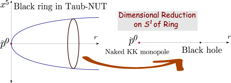
Figure 1: A Black ring away from the centre of Taub-NUT is projected down to a black hole and naked Kaluza-Klein magnetic monopole in four dimensions. The angular momentum carried in the compact dimension will translate to electric charge in four dimensions. An $AdS^{2}\times S^{2}\times U(1)$ near horizon geometry will project down to $AdS^{2}\times S^{2}$. On the other hand, an $AdS^{2}\times U(1)^{2}$ will go to $AdS^{2}\times U(1)$.

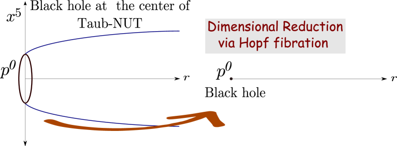
Figure 2: A black hole at the centre of Taub-NUT caries $NUT$ charge. Using the Hopf fibration it can be projected down to black hole carrying magnetic charge. A spherically symmetric black hole with near horizon geometry of $AdS^{2}\times S^{3}$ will project down to an $AdS^{2}\times S^{2}$. On the other hand, a rotating black hole with a $AdS^{2}\times U(1)^{2}$ geometry will go to $AdS^{2}\times U(1)$.

Since the entropy function analysis only depends on the near horizon geometry we will not be interested in the full geometry of Taub-NUT space. We will only be concerned with its influence on the near horizon geometry. The effect of the Taub-NUT charge is to introduce identifications so that the black hole horizon topology becomes $S^{3}/{\mathbb{Z}}_{p^{0}}$ and the black ring horizon topology becomes $S^{2}\times S^{1}/{\mathbb{Z}}_{{\tilde{p}}^{0}}$

We either use $\tilde{p}^{0}$, to denote the Taub-NUT charge of the space a black ring is sitting in, or $p^{0}$, to denote the charge of a black hole sitting at the centre of the space. In each case the $U(1)$ will be replaced by either $U(1)/\tilde{p}^{0}$ or $U(1)/{p}^{0}$. Unlike the black hole, the black ring does not carry Taub-NUT charge. Since we are only looking at the near horizon geometry, the only influence of the charge on the ring will be to induce an identification which we can impose this by hand. To encode asymptotically flat space we simply set the Taub-NUT charge to $1$ in both cases. For a unified presentation, we include ${p}^{0}$ and $\tilde{p}^{0}$ in the formulae below. Given this notation, when we consider black rings, we must remember to set $p^{0}=0$ and mod out the $U(1)$ by $\tilde{p}^{0}$. When considering black holes, $p^{0}$ is non-zero and, since we do need to mod out by hand, we set $\tilde{p}^{0}=1$.

For black holes, we can fibre the $U(1)$ over the $S^{2}$ to get $S^{3}/\mathbb{Z}_{p^{0}}$ while for the rings it will turn out that we can fibre the $U(1)$ over the $AdS_{2}$ to get $AdS_{3}/\mathbb{Z}_{\tilde{p}^{0}}$. These fibrations will only work for specific values of the radius of the Kaluza-Klein circle, $w$, depending on the radii of the base spaces, $S^{2}$ or $AdS^{2}$, and the parameters, $p^{0}$ or $e^{0}$ respectively. Even though we start out treating $w$ as an arbitrary parameter, we will see below that the “correct” value for $w$ will be dynamically generated by solving the equations of motion for $w$ coming from the entropy function analysis. The fibration which gives us $S^{3}$ is the standard Hopf fibration and the one for $AdS$, which is very similar, is discussed towards the end of Appendix C.

Now, to study the near horizon geometry of black holes and black rings in Taub-NUT space, with the required symmetries, we specialise our Kaluza-Klein ansatz, (2.2-2.4), to

$$ds^{2} =w^{-1}\left[v_{1}\left(-r^{2}dt^{2}+{\frac{dr^{2}}{r^{2}}}\right)+v_{2}\,\left(d\theta^{2}+\sin^{2}\theta d\phi^{2}\right)\right]$$

$$+w^{2}\left(d\psi+e^{0}\,rdt+p^{0}\cos\theta d\phi\right)^{2},$$ (3.1)

$${\bar{A}}^{I} =e^{I}\,rdt+{p^{I}\cos\theta}d\phi+a^{I}\left(d\psi+e^{0}\,rdt+p^{0}\cos\theta d\phi\right),$$ (3.2)

$${\bar{X}}^{S} =u^{S},$$ (3.3)

where the coordinates, $\theta$ and $\phi$ have periodicity $\pi$ and $2\pi$ respectively. The coordinate $\psi$ has periodicity $4\pi$ for black holes and $4\pi/\tilde{p}^{0}$ for black rings. This ansatz, (3.1-3.3), is consistent with the near horizon geometries of the solutions of [60, 61, 62, 63] as discussed in Appendix C.

Now that we have an appropriate five dimensional ansatz, we can construct the entropy function from the dimensionally reduced four dimensional Lagrangian. From the four dimensional action, we can evaluate the reduced Lagrangian, $f$, evaluated at the horizon subject to our ansatz. The entropy function is then given by the Legendre transformation of $f$ with respect to the electric fields and their conjugate charges.

The reduced four dimensional action, $f$, evaluated at the horizon is given by

$$f=\frac{1}{16\pi G_{4}}\int_{H}d\theta d\phi\sqrt{-g}{\cal L}=\frac{1}{16\pi}\left(\frac{4\pi}{\tilde{p}^{0}G_{5}}\right)\int_{H}d\theta d\phi\sqrt{-g}{\cal L}.$$ (3.4)

The equations of motion are equivalent to

$$f_{,v_{1}}=f_{,v_{2}}=f_{,w}=f_{,\vec{a}}=f_{,\vec{\Phi}}=0,$$ (3.5)

$$f_{,e^{i}}=Nq_{i},$$ (3.6)

where $e^{i}=(e^{0},e^{I})$ and $q_{i}$ are its (conveniently normalised) conjugate charges. We choose the the normalisation $N=4\pi/\tilde{p}^{0}G_{5}=1/G_{4}$. Using the ansatz, (3.1), we find

$$f ={\left(\frac{2\pi}{\tilde{p}^{0}G_{5}}\right)}\left\{\begin{array}[]{ll}v_{1}-v_{2}&-(v_{1}/v_{2})\left[\tfrac{1}{4}{w^{3}(p^{0})^{2}}+w{\bar{f}}_{IJ}(p^{I}+p^{0}a^{I})(p^{J}+p^{0}a^{J})\right]\\ &+(v_{2}/v_{1})\left[\tfrac{1}{4}{w^{3}(e^{0})^{2}}+w{\bar{f}}_{IJ}(e^{I}+e^{0}\,a^{I})(e^{J}+e^{0}\,a^{J})\right]\end{array}\right\}$$ (3.9)

$$+\left(\frac{24\pi}{\tilde{p}^{0}G_{5}}\right){\bar{c}}_{IJK}\left\{p^{I}e^{J}a^{K}+\tfrac{1}{2}(p^{0}e^{I}+e^{0}p^{I})a^{J}a^{K}+\tfrac{1}{3}p^{0}e^{0}a^{I}a^{J}a^{K}\right\},$$ (3.10)

while (3.6) gives the following relationship between the electric fields, $e^{i}$, and their conjugate charges $q_{i}$:

$$\hat{q}_{I} =(v_{2}/v_{1})w{\bar{f}}_{IJ}(e^{J}+e^{0}a^{J}),$$ (3.11)

$$\hat{q}_{0}-a^{I}\hat{q}_{I} =\left(v_{2}/v_{1}\right)(\tfrac{1}{4}w^{3}e^{0}),$$ (3.12)

where, $p^{i}=(p^{0},p^{I})$, $\tilde{f}_{ij}$ is given by (2.8) and the shifted charges, $\hat{q_{i}}$, are defined as

$$\hat{q}_{i} =q_{i}-\tilde{f}_{ij}p^{j}.$$ (3.13)

The entropy function is the Legendre transform of $f$ with respect to the charges $q_{i}$:

$${\cal E} =2\pi(Nq_{i}e^{i}-f).$$ (3.14)

In terms of ${\cal E}$ the equations of motion become

$${\cal E}_{,v_{1}}={\cal E}_{,v_{2}}={\cal E}_{,w}={\cal E}_{,\vec{a}}={\cal E}_{,\vec{\Phi}}={\cal E}_{,\vec{e}}=0.$$ (3.15)

Evaluating the entropy function gives

$${\cal E}=2\pi(Nq^{i}e_{i}-f)={4\pi^{2}\over\tilde{p}^{0}G_{5}}\left\{v_{2}-v_{1}+(v_{1}/v_{2})V_{eff}\right\},$$ (3.16)

where we have defined the effective potential

$$V_{eff} =f^{ij}\hat{q}_{i}\hat{q}_{j}+f_{ij}p^{i}p^{j}$$ (3.17)

where $f_{ij}$ is given by (2.7) and $f^{ij}$, the inverse of $f_{ij}$, is given by

$$f^{ij} =\bordermatrix{&0&J\cr 0&4w^{-3}&-4w^{-3}a^{J}\cr I&-4w^{-3}a^{I}&w^{-1}{\bar{f}}^{IJ}+4w^{-3}a^{I}a^{J}\cr},$$ (3.18)

where ${\bar{f}}^{IJ}$ is the inverse of ${\bar{f}}_{IJ}$. More explicitly, the effective potential is given by

$$V_{eff} =\tfrac{1}{4}w^{3}(p^{0})^{2}+4w^{-3}\{q_{0}-\tilde{f}_{0j}(\vec{a})p^{j}-a^{I}(q_{I}-\tilde{f}_{Ij}(\vec{a})p^{j}\}^{2}$$

$$+w{\bar{f}}_{IJ}(\vec{X})\{p^{I}+a^{I}p^{0}\}\{p^{J}+a^{J}p^{0}\}$$

$$+w^{-1}{\bar{f}}^{IJ}(\vec{X})\{q_{I}-\tilde{f}_{Ik}(\vec{a})p^{k}\}\{q_{J}-\tilde{f}_{Jl}(\vec{a})p^{l}\},$$ (3.19)

3.2 Charges

From a four dimensional perspective, the charges are simple to interpret — the $p^{i}$ are conventional magnetic charges and the $q^{i}$ are the conjugates to the electric field. Since we are using dimensional reduction to perform our calculations, it is easiest to work with these charges. When we write the gauge field in terms of a Kaluza-Klein ansatz, (3.2), from a five dimensional perspective, things are a little more complicated. We need to separately consider the charges $p^{0}$, $p^{I}$, $q^{0}$ and $q^{I}$.

The charge $p^{0}$ corresponds to the Taub-NUT charge while the $p^{I}$ are related to the dipole charge. When $p^{0}$ is zero, the charges $p^{I}$ correspond to dipole charges of the $S_{2}$ parameterised by $\theta$ and $\phi$. This is the case for the black ring solutions considered in section 3.4. On the other hand, when $p^{0}$ is non-zero, the flux through the $S_{2}$, in our conventions, goes like $p^{I}+a^{I}p^{0}$. It is this quantity should be interpreted as the dipole charge rather than $p^{I}$. So generally, the relationship between $p^{I}$ and the dipole charge will depend on the value of the axions, $a^{I}$ and the Taub-NUT charge. When we are considering black holes, we expect the dipole charge to be zero, but as we will see in section 3.5, the $p^{I}$ are non-zero. In this case they are simply to be interpreted as a quantity proportional to $a^{I}$.

The charge $q^{0}$ is related to the angular momentum while the $q^{I}$ are related to the electric charge. When $e^{0}$ is zero, the $q^{I}$ are simply the conjugates to the electric-field. Analogous to the dipole charges discussed above, when $e^{0}$ is non-zero, the electric field goes like $e^{I}+a^{I}e^{0}$. In this case, the relationship between $q^{I}$ and the electric charge depends on the values of $e^{0}$ and $a^{I}$.

3.3 Preliminary analysis

While the effective potential $V_{eff}$ is in general quite complicated, the dependence of the entropy function, (3.16), on the $S^{2}$ and $AdS^{2}$ radii is quite simple. Extremising the entropy function with respect to $v_{1}$ and $v_{2}$, one finds that, at the extremum,

$${\cal E}={4\pi^{2}\over\tilde{p}^{0}G_{5}}V_{eff}|_{\partial V=0},$$ (3.20)

with

$$v_{1}=v_{2}=V_{eff}|_{\partial V=0},$$ (3.21)

where the effective potential is to be evaluated at its extremum:

$${\partial_{\{w,\vec{a},\vec{X}\}}V_{eff}}=0.$$ (3.22)

From, (3.21), we see that the radii of the $S^{2}$ and $AdS^{2}$ are equal with the scale set by size of the charges.

As a check, we note that, the result, (3.20), agrees with the both the four and five Hawking-Bekenstein entropy since,

$$A_{H}^{(5)}=\int d\psi d\theta d\phi\sqrt{g_{\psi\psi}g_{\theta\theta}g_{\phi\phi}}={16\pi^{2}v_{2}}/{{\tilde{p}}^{0}}$$ (3.23)

so

$${\cal E}\stackrel{{\scriptstyle\scriptsize\begin{array}[]{c}(\ref{eq:v:sol})\\ (\ref{eq:area})\end{array}}}{{=}}{A_{H}^{(5)}\over 4G_{5}}\stackrel{{\scriptstyle(\ref{eq:G4vsG5})}}{{=}}{A_{H}^{(4)}\over 4G_{4}}=S_{BH}.$$ (3.24)

Notice that $w$ drops out of (3.24).

Finding extrema of the general effective potential, $V_{eff}$, given by (3.19) may in principle be possible but in practice not simple. In the following sections we consider simpler cases with only a subset of charges turned on.

3.4 Black rings

We are now really to specialise to the case of black rings. As discussed at the beginning of the section, for black rings, we take $p^{0}=0$ so that our $AdS_{2}\times U(1)\times S^{2}$ ansatz becomes

$$ds^{2} =w^{-1}\left[v_{1}\left(-r^{2}dt^{2}+{\frac{dr^{2}}{r^{2}}}\right)+v_{2}\,\left(d\theta^{2}+\sin^{2}\theta d\phi^{2}\right)\right]+w^{2}\left(d\psi+e^{0}\,rdt\right)^{2},$$ (3.25)

$${\bar{A}}^{I} =e^{I}\,rdt+{p^{I}\cos\theta}d\phi+a^{I}\left(d\psi+e^{0}\,rdt\right),$$ (3.26)

$${\bar{X}}^{S} =u^{S}.$$ (3.27)

In this case the gauge field (or in 4-D language the axion) equations simplify considerably and it is convenient to analyse them first. Varying $f$ with respect to $\vec{a}$ we find

$$d_{IJ}(e^{J}+e^{0}a^{J})=0$$ (3.28)

where $d_{IJ}=w{\bar{f}}_{IJ}e^{0}+6{\bar{c}}_{IJK}p^{K}$. Assuming $d_{IJ}$ has no zero eigenvalues, (3.28) implies that the electric field, $F^{J}_{tr}=e^{J}+e^{0}a^{J}$, is zero. Using (3.11,3.13) this in turn implies $\hat{q}_{I}=0$ which, using (2.8,3.13), allows us to solve for the axions:

$$a^{K}={\bar{c}}^{KJ}q_{J},$$ (3.29)

where ${\bar{c}}^{KJ}$ is the inverse of

$${\bar{c}}_{IJ}=6{\bar{c}}_{IJK}p^{K}.$$ (3.30)

Notice that ${\bar{c}}_{IJ}$ is equal to the sub-matrix, $\tilde{f}_{IJ}$, with $a^{K}$ replaced by $p^{K}$. Now substituting (3.29) into the definition of $\hat{q}_{0}$ we find:

$$\hat{q}_{0}=q_{0}-\tfrac{1}{2}{\bar{c}}^{IJ}q_{I}q_{J}.$$ (3.31)

So, eliminating the axions and using $\hat{q}_{I}=0$, the effective potential becomes

$$V_{eff}=w{\bar{f}}_{IJ}p^{I}p^{J}+(4w^{-3})(\hat{q}_{0})^{2}.$$ (3.32)

Using $\partial_{w}V_{eff}=0$ we find

$$w^{4}={12\hat{q}_{0}^{2}\over V_{M}}$$ (3.33)

where we have defined the magnetic potential, $V_{M}={\bar{f}}_{IJ}p^{I}p^{J}$. So

$$V_{eff}={4\over 3}wV_{M}=16w^{-3}(\hat{q}_{0})^{2}$$ (3.34)

Eliminating $w$ from $V_{eff}$ we get

$${\cal E}={8\pi^{2}\over\tilde{p}^{0}G_{5}}\sqrt{\hat{q}_{0}(\tfrac{4}{3}V_{M})^{3\over 2}}.$$ (3.35)

We note that

$$e_{0}^{2}w^{2}=v_{1}w^{-1}$$ (3.36)

which, we see by comparison with (C.40), means that we have a $S^{2}\times AdS_{3}/\mathbb{Z}_{\tilde{p}^{0}}$ near horizon geometry. Finally, using (3.21,3.34,3.36) we can also write the entropy as

$${\cal E}={4\pi^{2}\over\tilde{p}^{0}G_{5}}{(\tfrac{4}{3}V_{M})^{3\over 2}}{(e^{0})^{-1}}$$ (3.37)

3.5 Static 5-d black holes

We now consider five dimensional static spherically symmetric black holes. Since they are not rotating we take $e^{0}=0$. This is in some sense “dual” to taking $p^{0}=0$ for black rings. To examine this analogy further, we will relax the natural assumption of an $AdS_{2}\times S^{3}$ geometry to $AdS_{2}\times S^{2}\times U(1)$. We will see that the analysis for the black holes is very similar to the analysis of the black rings with the magnetic potential replaced by an electric potential. Once we solve the equations of motion we recover an $AdS_{2}\times S^{3}$ geometry via the Hopf fibration. This is analogous to the black ring where we got $AdS_{3}\times S^{2}$ with the $U(1)$ fibred over the $AdS_{2}$ rather than the $S^{2}$.

With $e^{0}=0$, our ansatz becomes

$$ds^{2} =w^{-1}\left[v_{1}\left(-r^{2}dt^{2}+{\frac{dr^{2}}{r^{2}}}\right)+v_{2}\,\left(d\theta^{2}+\sin^{2}\theta d\phi^{2}\right)\right]+w^{2}\left(d\psi+p^{0}\cos\theta d\phi\right)^{2},$$ (3.38)

$$A^{I} =e^{I}\,rdt+{p^{I}\cos\theta}d\phi+a^{I}\left(d\psi+p^{0}\cos\theta d\phi\right),$$ (3.39)

$$\Phi^{S} =u^{S}.$$ (3.40)

In this case the gauge field equation becomes

$$\tilde{d}_{IJ}(p^{J}+p^{0}a^{J})=0$$ (3.41)

where $\tilde{d}_{IJ}=w{\bar{f}}_{IJ}p^{0}-6{\bar{c}}_{IJK}e^{K}$. Assuming $\tilde{d}_{IJ}$ has no zero eigenvalues, (3.41) implies $F^{I}_{\theta\phi}=0$, which, together with (3.12,3.13), gives

$$\hat{q}_{0}-a^{I}\hat{q}_{i} =0$$ (3.42)

$$a^{K} =-p^{K}/p^{0},$$ (3.43)

$$\hat{q}_{I} =q_{I}+3{\bar{c}}_{IJK}p^{J}p^{K}/p^{0}$$ (3.44)

and the effective potential becomes

$$V_{eff}=(\tfrac{1}{4}w^{3})(p_{0})^{2}+w^{-1}{\bar{f}}^{IJ}\hat{q}_{I}\hat{q}_{J}.$$ (3.45)

Using $\partial_{w}V_{eff}=0$ we find

$$w^{4}={4V_{E}\over 3p_{0}^{2}}$$ (3.46)

where we have defined the electric potential $V_{E}=\bar{f}^{IJ}\hat{q}_{I}\hat{q}_{J}$. So

$$V_{eff}={4\over 3}w^{-1}V_{E}=w^{3}(p^{0})^{2}$$ (3.47)

Eliminating $w$ from ${\cal E}$ we find

$${\cal E}={4\pi^{2}\over G_{5}}\sqrt{p_{0}(\tfrac{4}{3}V_{E})^{3\over 2}}.$$ (3.48)

We note that, analogous to the ring case where we had $e_{0}^{2}w^{2}=v_{1}w^{-1}$,

$$p_{0}^{2}w^{2}=v_{2}w^{-1}$$ (3.49)

which, via the Hopf fibration, gives us an $AdS_{2}\times S^{3}/\mathbb{Z}_{p^{0}}$ near horizon geometry.

3.6 Very Special Geometry

We now consider the explicit example of ${\cal N}=2$ supergravity in five dimensions corresponding to M-theory on a Calabi-Yau threefold – this gives what has been called real or very special geometry [64, 65, 66, 67, 68, 69, 70]. Some properties of very special geometry which we use are recorded in Appendix B. Building on the general results of the previous sections, to find the attractor values of the scalars and the entropy we just need to extremise the relevant magnetic or electric potentials.

3.6.1 Black rings and very special geometry

For very special geometry, the magnetic potential is given by

$$V_{M}=\bar{f}_{IJ}p^{I}p^{J}\stackrel{{\scriptstyle(\ref{eq:hvsf})}}{{=}}\tfrac{1}{2}H_{IJ}p^{I}p^{J}$$ (3.50)

where the properties of $H_{IJ}$ can be found in Appendix B.

Extremising the magnetic potential gives

$$\partial_{i}V_{M}=\tfrac{1}{2}\partial_{i}(H_{IJ}p^{I}p^{J})\stackrel{{\scriptstyle(\ref{special:lower:2})}}{{=}}\tfrac{1}{4}\partial_{i}(p_{I}p^{I})=0$$ (3.51)

These equations have a solution

$$\lambda X_{I}=p_{I}$$ (3.52)

This condition follows from one of the BPS conditions found in [33]. To see that (3.52) is indeed a solution, we insert it into (3.51), which gives

$$\partial_{i}(p_{I}p^{I}) = \partial_{i}(p_{I})p^{I}$$ (3.53)

$$\stackrel{{\scriptstyle(\ref{BPS:anz})}}{{=}} \lambda\partial_{i}(X_{I})p^{I}$$ (3.54)

$$\stackrel{{\scriptstyle(\ref{special:covariant})}}{{=}} -2\lambda H_{IJ}p^{I}\partial_{i}(X^{J})$$ (3.55)

$$\stackrel{{\scriptstyle(\ref{special:lower})}}{{=}} -\lambda p_{J}\partial_{i}(X^{J})$$ (3.56)

$$\stackrel{{\scriptstyle(\ref{BPS:anz})}}{{=}} -\lambda^{2}X_{J}\partial_{i}(X^{J})\stackrel{{\scriptstyle(\ref{X:norm:2})}}{{=}}0$$ (3.57)

We can fix the constant $\lambda$ using (B.3) which gives

$$X_{I}=\frac{p_{I}}{(\frac{1}{6}C_{IJK}p^{I}p^{J}p^{K})^{\frac{1}{3}}}$$ (3.58)

so finally we get for $X^{I}$,

$$X^{I}=\frac{p^{I}}{({1\over 6}C_{IJK}p^{I}p^{J}p^{K})^{\frac{1}{3}}}$$ (3.59)

and

$$V_{M}|_{\partial V=0} =\tfrac{1}{2}H_{IJ}p^{I}p^{J}=\tfrac{1}{2}\lambda^{2}H_{IJ}X^{I}X^{J}={3\over 4}\lambda^{2}$$ (3.60)

$$=\frac{3}{4}\left(\frac{1}{6}C_{IJK}p^{I}p^{J}p^{K}\right)^{\frac{2}{3}}$$ (3.61)

This is the supersymmetric solution of [33] derived from the BPS attractor equations.

Notice that (3.54) can be rewritten as extremising the magnetic central charge, $Z_{M}=X_{I}p^{I}$:

$$\partial_{i}(X_{I})p^{I}=\partial_{i}Z_{M}=0$$ (3.62)

So we see that $\partial_{i}V_{M}=0$ together with the BPS condition (3.52) implies $Z_{M}$ extremised. The converse is not necessarily true suggesting there are non-BPS black ring extrema of $V_{M}$ — this is discussed below.

Now, from (3.61,3.35) we find that the entropy is

$${\cal E}={8\pi^{2}\over\tilde{p}^{0}G_{5}}\sqrt{{\hat{q}_{0}}(\tfrac{1}{6}C_{IJK}p^{I}p^{J}p^{K})}={4\pi^{2}\over\tilde{p}^{0}G_{5}}{(\tfrac{1}{6}C_{IJK}p^{I}p^{J}p^{K})}{(e^{0})^{-1}}$$ (3.63)

As discussed in Appendix C this gives the correct entropy for the special case of the ring solution of [62].

3.6.2 Static black holes and very special geometry

The analysis for these black holes is analogous to the black rings. From the attractor equations for a static black hole, governed by

$$V_{E}=\bar{f}^{IJ}\hat{q}_{I}\hat{q}_{J}=2H^{IJ}\hat{q}_{I}\hat{q}_{J}$$ (3.64)

we will get the equation:

$$\partial_{i}V_{E}=2\partial_{i}(H^{IJ}\hat{q}_{I}\hat{q}_{J})=\partial_{i}(\hat{q}^{I}\hat{q}_{I})=0$$ (3.65)

This will have similar solutions

$$X^{I}=\frac{\hat{q}^{I}}{({1\over 6}C_{IJK}\hat{q}^{I}\hat{q}^{J}\hat{q}^{K})^{\frac{1}{3}}}$$ (3.66)

Similarly, extremising the electric central charge $Z_{e}$ of [33] together with the BPS condition implies $V_{E}$ is extremised. The converse is not necessarily true suggesting there are non-BPS black hole extrema of $V_{E}$ as noted in [71].

In a similar fashion to the black ring case, we find that the entropy is given by

$${\cal E}=\frac{\pi^{2}}{2G_{5}}\sqrt{{p^{0}}(\tfrac{1}{6}C^{IJK}[16{\hat{q}}_{I}][16{\hat{q}}_{J}][16{\hat{q}}_{K}])}.$$ (3.67)

which, modulo a different normalisation for the charges, is the same as the entropy quoted in [71] (albeit modified due to the presence of a Taub-NUT charge). As shown in Appendix D, our charges, $\hat{q}_{I}$, are related to those of [71] by

$${16\hat{q}}_{I}=Q_{I}.$$ (3.68)

The appearance of the shifted charge ${\hat{q}}_{I}$ rather than $q_{I}$ is due to the Chern-Simons term.

3.6.3 Non-supersymmetric solutions of very special geometry

In 4 dimensional ${\cal N}=2$ special geometry we can write $V_{eff}$ or the “blackhole potential function” as [5]

$$V_{BH}=|Z|^{2}+|DZ|^{2}.$$ (3.69)

As noted in [5] and [4] (in slightly different notation), for BPS solutions, each term of the potential is separately extremised while for non-BPS solutions $V_{BH}$ is extremised but $DZ\neq 0$. It is perhaps not surprising that a similar thing happens in very special geometry. In fact, this generalisation of the non-BPS attractor equations to five dimensional static black holes has already be shown in [71] using a reduced Lagrangian approach.

The electric potential $V_{E}$ can be written

$$\tfrac{1}{2}V_{E}=H^{IJ}\hat{q}_{J}\hat{q}_{J}=H^{IJ}(D_{I}\hat{Z}_{E})(D_{J}\hat{Z}_{E})+\tfrac{2}{3}(\hat{Z}_{E})^{2}.$$ (3.70)

Solving $D_{I}V_{E}=0$ we find a BPS solution, $D_{I}\hat{Z}_{E}=0$, and another solution

$$\tfrac{2}{3}H_{IJ}\hat{Z}_{E}+D_{I}D_{J}\hat{Z}_{E}=0.$$ (3.71)

Similarly, we find the magnetic potential, $V_{M}$, can be written

$$2V_{M}=H_{IJ}p^{I}p^{J}=\tfrac{1}{3}Z_{M}^{2}+H^{IJ}D_{I}Z_{M}D_{J}Z_{M}$$ (3.72)

and solving $D_{I}V_{M}=0$ we find a BPS solution, $D_{I}Z_{M}=0$, and another solution

$$\tfrac{1}{3}H_{IJ}Z_{M}+D_{I}D_{J}Z_{M}=0.$$ (3.73)

We conjecture one can obtain some five dimensional non-SUSY solutions by lifting non-SUSY solutions in four dimensions which have $AdS_{2}\times S^{2}$ near horizon geometries using the $4D$-$5D$ lift. Furthermore the analysis of [4] should go through so that for such solutions to exist we require that extremum of $V_{eff}$ is a minimum – in other words the matrix

$$\left.{\partial^{2}V_{eff}\over\partial\Phi^{S}\partial\Phi^{T}}\right|_{\partial V=0}>0$$ (3.74)

should have non-zero eigenvalues.

4 General Entropy function

We now relax our symmetry assumptions to $AdS_{2}\times U(1)^{2}$, taking the following ansatz

$$ds^{2} =w^{-1}(\theta)\Omega^{2}(\theta)e^{2\Psi(\theta)}\left(-r^{2}dt^{2}+{dr^{2}\over r^{2}}+\beta^{2}d\theta^{2}\right)+w^{-1}(\theta)e^{-2\Psi(\theta)}(d\phi+e_{\phi}rdt)^{2}$$

$$+w^{2}(\theta)(d\psi+e_{0}rdt+b_{0}(\theta)d\phi)^{2}$$ (4.1)

$$A^{I} =e^{I}rdt+b^{I}(\theta)(d\phi+e_{\phi}rdt)+a^{I}(\theta)(d\psi+e_{0}rdt+b_{0}(\theta)d\phi)$$ (4.2)

$$\phi^{S} =u^{S}(\theta).$$ (4.3)

Now, using (2.5) and then following [40], the entropy function is

$${\cal E} \equiv 2\pi(J_{\phi}e_{\phi}+\vec{q}\cdot\vec{e}-\int d\theta d\phi\sqrt{-\det g}\,{\cal L})$$ (4.4)

$$=2\pi(J_{\phi}e_{\phi}+\vec{q}\cdot\vec{e})$$

$$-{\pi^{2}\over\tilde{p}_{0}G_{5}}\int d\theta\,\Bigg{[}2\Omega^{-1}\beta^{-1}(\Omega^{\prime})^{2}-2\Omega\beta-2\Omega\beta^{-1}(\Psi^{\prime})^{2}+{1\over 2}\alpha^{2}\Omega^{-1}\beta e^{-4\Psi}-\beta^{-1}\Omega h_{rs}(\vec{u})u_{r}^{\prime}u_{s}^{\prime}$$

$$+4\tilde{f}_{ij}(\vec{u})(e_{i}-\alpha b_{i})b_{j}^{\prime}+2f_{ij}(\vec{u})\left\{\beta\Omega^{-1}e^{-2\Psi}(e_{i}-\alpha b_{i})(e_{j}-\alpha b_{j})-\beta^{-1}\Omega e^{2\Psi}b_{i}^{\prime}b_{j}^{\prime}\right\}\Bigg{]}$$

$$+{2\pi^{2}\over\tilde{p}_{0}G_{5}}\,\left[\Omega^{2}e^{2\Psi}\sin\theta(\Psi^{\prime}+2\Omega^{\prime}/\Omega)\right]_{\theta=0}^{\theta=\pi}.$$ (4.5)

where $f_{ij}$, $\tilde{f}_{ij}$,$h_{rs}$ and $u^{s}$ related to five dimensional quantities as discussed in section 2. Now extremising the entropy function gives us differential equations.

Using the near horizon geometry of the non-SUSY black ring of [72], which we evaluate in Appendix E, we find that the entropy function gives the correct entropy.

Acknowledgements: We would like to thank Sandip Trivedi for helpful discussions and invaluable comments on the draft and Ashoke Sen for useful comments and suggestions. We thank the organisers of the conference “ISM’06”, held in Dec 2006, where some part of the work was done. We also thank the people of India for supporting research in String theory.

Appendix A Dimensional reduction

In this section present some details of the dimensional reduction of the Chern-Simons term. We start with the five dimensional gauge-fields which we assume are independent of the fifth direction:

$$\bar{A}^{I} = \bar{A}^{I}_{\mu}dx^{\mu}+\bar{A}^{I}_{y}dy$$ (A.6)

$$= A^{I}_{\mu}dx^{\mu}+a^{I}(x^{\mu})\left(dy+A^{0}_{\mu}dx^{\mu}\right).$$ (A.7)

From these definitions we can relate the five dimensional gauge field strength to four dimensional quantities as follows

$$\bar{F}_{\mu\nu}^{I} =F_{\mu\nu}^{I}+a^{I}F_{\mu\nu}^{0}+(\partial_{\mu}a^{I})A_{\nu}^{0}-(\partial_{\nu}a^{I})A_{\mu}^{0},$$ (A.8)

$$\bar{F}_{\nu y}^{I} =\partial_{\nu}a^{I},$$ (A.9)

where

$$F_{\mu\nu}^{i}=\partial_{\mu}A_{\nu}^{i}-\partial_{\nu}A_{\mu}^{i}\qquad i=I\mbox{ or }0.$$ (A.10)

We can now write a five dimensional Chern-Simons term,

$$\sqrt{-\bar{g}}{\cal L}_{CS}=\;\bar{c}_{IJK}{\tilde{\epsilon}}^{\bar{\mu}\bar{\nu}\bar{\alpha}\bar{\beta}\bar{\delta}}\bar{A}^{I}_{\bar{\mu}}\bar{F}^{J}_{\bar{\alpha}\bar{\beta}}\bar{F}^{K}_{\bar{\mu}\bar{\nu}},$$ (A.11)

as

$$\sqrt{-\bar{g}}{\cal L}_{CS} =\bar{c}_{IJK}\tilde{\epsilon}^{\mu\nu\alpha\beta}(\bar{A}^{I}_{y}\bar{F}^{J}_{\mu\nu}\bar{F}^{K}_{\alpha\beta}+4\bar{A}^{I}_{\mu}\bar{F}^{J}_{\nu y}\bar{F}^{K}_{\alpha\beta})$$ (A.12)

$${\rightarrow}\;3\bar{c}_{IJK}\tilde{\epsilon}^{\mu\nu\alpha\beta}a^{I}\bar{F}^{J}_{\mu\nu}\bar{F}^{K}_{\alpha\beta}$$ (A.13)

$$=3\bar{c}_{IJK}\tilde{\epsilon}^{\mu\nu\alpha\beta}\left(a^{I}(F_{\mu\nu}^{J}+a^{J}F_{\mu\nu}^{0})(F_{\alpha\beta}^{K}+a^{K}F_{\alpha\beta}^{0})+\cancel{4a^{J}_{,\mu}a^{K}_{,\alpha}A_{\nu}^{0}A_{\beta}^{0}}\right)$$

$$+3\bar{c}_{IJK}\tilde{\epsilon}^{\mu\nu\alpha\beta}\Big{(}\underbrace{\tfrac{4}{2}(a^{I}a^{J})_{,\mu}A_{\nu}^{0}F_{\alpha\beta}^{K}}_{\rightarrow-a^{I}a^{J}F_{\mu\nu}^{0}F_{\alpha\beta}^{K}}+\underbrace{\tfrac{4}{3}(a^{I}a^{J}a^{K})_{,\mu}A_{\nu}^{0}F_{\alpha\beta}^{0}}_{\rightarrow-\tfrac{2}{3}a^{I}a^{J}a^{K}F_{\mu\nu}^{0}F_{\alpha\beta}^{0}}\Big{)}$$ (A.14)

$$=3\bar{c}_{IJK}\tilde{\epsilon}^{\mu\nu\alpha\beta}\left(a^{I}F_{\mu\nu}^{J}F_{\alpha\beta}^{K}+\tfrac{1}{2}a^{I}a^{J}(F_{\mu\nu}^{K}F_{\alpha\beta}^{0}+F_{\mu\nu}^{0}F_{\alpha\beta}^{K})+\tfrac{1}{3}a^{I}a^{J}a^{K}F_{\mu\nu}^{0}F_{\alpha\beta}^{0}\right)$$ (A.15)

$$=(\tfrac{1}{2}\tilde{f}_{ij})F^{i}_{\mu\nu}F^{j}_{\alpha\beta}\tilde{\epsilon}^{\mu\nu\alpha\beta}$$ (A.16)

where the arrow, “$\rightarrow$”, denotes the use of integration by parts, and $\tilde{\epsilon}^{01234}=\tilde{\epsilon}^{0123}=1$, are the completely antisymmetric Levi-Civita symbols.

Appendix B Notes on Very Special Geometry

Here we collect some useful relations and define some notation from very special geometry along the lines of [33, 71], which are used in section 3.6.

• We take our CY₃ to have Hodge numbers $h^{1,1}$ with the index $I\in{1,2,\ldots,h^{1,1}}$.

• The Kähler moduli, $X^{I}$ which are real, correspond to the volumes of the 2-cycles.

• $C_{IJK}$ are the triple intersection numbers. They are related to the couplings defined in (2.1) by

  $$C_{IJK}={4!}\bar{c}_{IJK}$$ (B.1)

• The volumes of the 4-cycles $\Omega_{I}$ are given by

  $$X_{I}={1\over 2}C_{IJK}X^{J}X^{K}~{}.$$ (B.2)

• The prepotential is given by

  $${\cal V}={1\over 6}C_{IJK}X^{I}X^{J}X^{K}=1$$ (B.3)

• The volume constraint (B.3) implies there are $n_{v}=h^{1,1}-1$ independent vector-multiplets.

• denote the independent vector-multiplet scalars as $\phi^{i}$, and the corresponding derivatives $\partial_{i}={\partial\over\partial\phi^{i}}$.

• The kinetic terms for the gauge fields are governed by the metric

  $${H_{IJ}=-\tfrac{1}{2}\left.\partial_{I}\partial_{J}\ln{\cal V}\right|_{{\cal V}=1}=-\tfrac{1}{2}(C_{IJK}X^{K}-X_{I}X_{J})~{},}$$ (B.4)

  where we use the notation for derivatives: $\partial_{I}={\partial\over\partial X^{I}}$. In terms of the couplings used in (2.1) we have

  $$H_{IJ}={\bar{h}}_{IJ}=2\bar{f}_{IJ}$$ (B.5)

• The electric central charge is given by

  $$Z_{E}=X^{I}q_{I}.$$ (B.6)

  We generalise this to

  $$\hat{Z}_{E}=X^{I}\hat{q}_{I}.$$ (B.7)

• The magnetic central charge is given by

  $$Z_{M}=X_{I}p^{I}.$$ (B.8)

• From (B.2) it follows that

  $${X_{I}X^{I}=3~{},}$$ (B.9)

  so

  $${X^{I}\partial_{i}X_{I}=\partial_{i}X^{I}X_{I}=0~{}.}$$ (B.10)

  which in turn together with (B.4) gives

  $$\quad X_{I} =2H_{IJ}X^{J}~{},$$ (B.11)

  $$\partial_{i}X_{I} =-2H_{IJ}\partial_{i}X^{J}~{}.$$ (B.12)

• As suggested by, (B.11), we will use $2H_{IJ}$ to lower indices, so for example,

  $$p_{I}=2H_{IJ}p^{J},$$ (B.13)

  which in turn implies we should raise indices with $\tfrac{1}{2}H^{IJ}$,

  $$q^{I}=\tfrac{1}{2}H^{IJ}q_{J}$$ (B.14)

  where $H^{IJ}$ is the inverse of $H_{IJ}$.

• In order to take the volume constraint (B.3) into account, it is convenient to define a covariant derivative $D_{I}$,

  $$D_{I}f=(\partial_{I}-\tfrac{1}{3}(\partial_{I}\ln{\cal V})|_{{\cal V}=1})f.$$ (B.15)

  Rather than extremise with respect to the real degrees of freedom using $\partial_{i}$, we can take covariant derivatives.

Appendix C Supersymmetric black ring near horizon geometry

Here, we will consider the black ring solution of [60], and find the near horizon limit of the metric and the gauge fields. This will enable us to compare with the charges defined in section 3.1.

As [60] follows the conventions of [73] the relevant Lagrangian is

$${\cal L}=R-\tilde{F}_{\mu\nu}\tilde{F}^{\mu\nu}-\tfrac{2}{3\sqrt{3}}\tilde{F}_{\alpha\beta}\tilde{F}_{\mu\nu}\tilde{A}_{\gamma}\epsilon^{\alpha\beta\mu\nu\gamma}.$$ (C.1)

We can obtain this action from very special geometry by taking, $n_{v}=3$ with the gauge fields equal to each other, $F^{I}_{\mu\nu}=F_{\mu\nu}$, fixing the scalars at their attractor value (3.58), and taking

$$C_{IJK}=|\epsilon_{IJK}|$$ (C.2)

where $\epsilon_{IJK}$ is the Levi-Civita symbol. This gives

$$X^{I}=1,\qquad H_{IJ}=(\tfrac{1}{2},\tfrac{1}{2},\tfrac{1}{2}),$$ (C.3)

and the Lagrangian becomes

$${\cal L}=R-\tfrac{3}{4}{F}_{\mu\nu}{F}^{\mu\nu}-\tfrac{1}{4}{F}_{\alpha\beta}{F}_{\mu\nu}{A}_{\gamma}\epsilon^{\alpha\beta\mu\nu\gamma}.$$ (C.4)

Comparing (C.1) and (C.4) we find

$$\tilde{A}_{\mu}=\tfrac{\sqrt{3}}{2}{A}_{\mu}$$ (C.5)

Now, the metric for the black ring solution of [60] is

$$ds^{2}=-f^{2}(dt+\omega)^{2}+f^{-1}ds^{2}(M_{4})\,,$$ (C.6)

where

$$f^{-1}=1+\frac{Q-q^{2}}{2R^{2}}(x-y)-\frac{q^{2}}{4R^{2}}(x^{2}-y^{2})$$ (C.7)

$$ds^{2}(\mathbb{R}^{4})=\frac{R^{2}}{(x-y)^{2}}\left\{\frac{dy^{2}}{y^{2}-1}+(y^{2}-1)d\vartheta^{2}+\frac{dx^{2}}{1-x^{2}}+(1-x^{2})d\phi^{2}\right\}$$ (C.8)

and $\omega=\omega_{\vartheta}(x,y)d\vartheta+\omega_{\phi}(x,y)d\phi$ with

$$\omega_{\phi} =-\frac{q}{8R^{2}}(1-x^{2})\left[3Q-q^{2}(3+x+y)\right]\,,$$ (C.9)

$$\omega_{\vartheta} =\frac{3}{2}q(1+y)+\frac{q}{8R^{2}}(1-y^{2})\left[3Q-q^{2}(3+x+y)\right]\,.$$ (C.10)

The variables $\vartheta$ and $\phi$ have period $2\pi$, while $-1\leq x\leq 1$ and $\infty<y\leq-1$. The gauge field is expressed as,

$$\tilde{A}=\frac{\sqrt{3}}{2}\left[f\,(dt+\omega)-\frac{q}{2}((1+x)\,d\phi+(1+y)\,d\vartheta)\right]\,.$$ (C.11)

The ADM charges are given by

$$M =\frac{3\pi}{4G}Q\,,\qquad J_{\phi}=\frac{\pi}{8G}\,q\,(3Q-q^{2})\,,$$

$$J_{\vartheta} =\frac{\pi}{8G}\,q\,(6R^{2}+3Q-q^{2})\,.$$ (C.12)

Near Horizon Geometry

In these coordinates, the horizon lies at $y\rightarrow-\infty$. To examine the near horizon geometry, it is convenient to define a new coordinate $r=-R/y$ (so the horizon is at $r=0$). Then consider a coordinate transformation of the form

$$dt =dv-B(r)dr,$$

$$d\phi =d\phi^{\prime}-C(r)dr,$$ (C.13)

$$d\vartheta =d\vartheta^{\prime}-C(r)dr,$$ (C.14)

where

$$B(r)=\frac{B_{2}}{r^{2}}+\frac{B_{1}}{r}+B_{0},\qquad C(r)=\frac{C_{1}}{r}+C_{0}.$$ (C.15)

where $B_{2}=q^{2}L/(4R)$ and $C_{1}=-q/(2L)$, with

$$L\equiv\sqrt{3\left[\frac{(Q-q^{2})^{2}}{4q^{2}}-R^{2}\right]},$$ (C.16)

and

$$B_{1}=(Q+2q^{2})/(4L)+L(Q-q^{2})/(3R^{2})$$

$$C_{0}=-(Q-q^{2})^{3}/(8q^{3}RL^{3})$$

$$B_{0}=q^{2}L/(8R^{3})+2L/(3R)-R/(2L)+3R^{3}/(2L^{3})+3(Q-q^{2})^{3}/(16q^{2}RL^{3})$$

The metric (C.8) becomes

$$ds^{2} =-\frac{16r^{4}}{q^{4}}dv^{2}+\frac{2R}{L}dvdr+\frac{4r^{3}\sin^{2}\theta}{Rq}dvd\phi^{\prime}+\frac{4Rr}{q}dvd\vartheta^{\prime}+\frac{3qr\sin^{2}\theta}{L}drd\phi^{\prime}$$

$$+2\Big{[}\frac{qL}{2R}\cos\theta+\frac{3qR}{2L}+\frac{(Q-q^{2})(3R^{2}-2L^{2})}{3qRL}\Big{]}drd\vartheta^{\prime}$$

$$+L^{2}d{\vartheta^{\prime}}^{2}+\frac{q^{2}}{4}\left[d\theta^{2}+\sin^{2}\theta\left(d\phi^{\prime}-d\vartheta^{\prime}\right)^{2}\right]+\ldots$$ (C.17)

where we have neglected terms which will disappear when we take the near horizon limit:

$$r=\epsilon L\tilde{r}/R,\;v=\tilde{v}/\epsilon,\;\epsilon\rightarrow 0.$$ (C.18)

The gauge field (C.11) becomes:

$$\tilde{A} =\tfrac{1}{2}{\sqrt{3}}\Big{[}f\,(dv+\omega^{\prime})-\tfrac{1}{2}{q}\left(\{1+x\}\,d\phi^{\prime}+\{1+y\}\,d\vartheta^{\prime}\right)$$ (C.19)

$$-\left(fB+C\left\{f\omega_{\phi}+f\omega_{\vartheta}-\tfrac{1}{2}{q}(1+x)-\tfrac{1}{2}{q}(1-{R}/{r})\right\}\right)dr\Big{]}$$ (C.20)

with $\omega^{\prime}=\omega_{\vartheta}d\vartheta^{\prime}+\omega_{\phi}d\phi^{\prime}$ In the limit of small $r$

$$f =\frac{1}{1+x(f_{1}-f_{2}x)+f_{1}r^{-1}+f_{2}r^{-2}}$$ (C.21)

$$=\frac{r^{2}}{f_{2}}\left(1-f_{1}f_{2}^{-1}r+\left(f_{1}^{2}f_{2}^{-1}-1+x(x-f_{1}f_{2}^{-1})\right)f_{2}^{-1}r^{2}+\mathcal{O}\left(r^{3}\right)\right)$$ (C.22)

where $f_{1}=(Q-q^{2})/2R^{2}$ and $f_{2}=q^{2}/4R^{2}$. Expanding $\omega$ in the limit of small $r$, we have,

$$\omega_{\phi} =\left\{-\frac{q^{3}\left(1-x^{2}\right)}{8R}\right\}\frac{1}{r}+\left\{\frac{q\left(xq^{2}+3q^{2}-3Q\right)\left(1-x^{2}\right)}{8R^{2}}\right\}$$ (C.23)

$$\omega_{\vartheta} =\left\{-\frac{q^{3}R}{8}\right\}\frac{1}{r^{3}}+\left\{\frac{xq^{3}}{8}+\frac{3q^{3}}{8}-\frac{3Qq}{8}\right\}\frac{1}{r^{2}}+\left\{\frac{q^{3}}{8R}-\frac{3qR}{2}\right\}\frac{1}{r}$$

$$+\left\{-\frac{xq^{3}}{8R^{2}}-\frac{3q^{3}}{8R^{2}}+\frac{3Qq}{8R^{2}}+\frac{3q}{2}\right\}$$ (C.24)

Expanding out the gauge field (neglecting some terms which can be gauged away) we obtain:

$$\tilde{A} =\tfrac{1}{2}{\sqrt{3}}\left\{-\left[{q\over 2}+{Q\over 2q}+\mathcal{O}(r)\right]d\vartheta^{\prime}+\left[-\frac{q}{2}\left(x+1\right)+\mathcal{O}(r)\right]d\chi\right.$$ (C.25)

$$+\left.\left[\frac{4}{q^{2}}r^{2}+\mathcal{O}(r^{3})\right]dv+\left[c_{r}x\,r+\mathcal{O}(r^{2})\right]dr\right\}$$

where $\chi=\phi-\vartheta$ and

$$c_{r}=\frac{L\left(R^{2}\left(2R^{4}-3\right)q^{4}+\left(-4QR^{6}+6QR^{2}+2\right)q^{2}+Q^{2}R^{2}\left(2R^{4}-3\right)\right)}{2q^{2}}$$ (C.26)

Finally taking the near-horizon limit (C.18), letting $x=-\cos\theta$, $\chi\rightarrow\phi$ and $\vartheta^{\prime}\rightarrow\psi/2$, we obtain

$$\tilde{A}=-\frac{\sqrt{3}}{8}\left[{q}+{Q\over q}\right]d\psi+\frac{\sqrt{3}q}{4}\left(\cos\theta-1\right)d\phi$$ (C.27)

So using (C.5) to compare (C.27) with (2.3,3.2) we get

$$p={p^{I}}={\frac{q}{2}}.$$ (C.28)

Taking the same near horizon limit for the metric we obtain

$$ds^{2}=2d\tilde{v}d\tilde{r}+\frac{4L}{q}\tilde{r}d\tilde{v}d\vartheta^{\prime}+L^{2}d\vartheta^{\prime 2}+\frac{q^{2}}{4}\left[d\theta^{2}+\sin^{2}\theta d\phi^{2}\right]$$ (C.29)

Let us for the moment consider the metric for constant $\theta$ and $\chi$. If we perform the coordinate transformation

$$d\vartheta^{\prime} =d\vartheta-\frac{q}{2L}\frac{d\tilde{r}}{\tilde{r}}$$ (C.30)

$$d\tilde{v} =dt+\frac{q^{2}}{4}\frac{d\tilde{r}}{\tilde{r}^{2}}$$ (C.31)

we get

$$ds^{2}=\frac{4L}{q}\tilde{r}dtd\vartheta+L^{2}d\vartheta^{2}+\frac{q^{2}}{4}\frac{d\tilde{r}}{\tilde{r}^{2}}$$ (C.32)

Letting

$$dt=dt^{\prime}+\frac{q}{2}d\vartheta$$ (C.33)

we obtain the more familiar form of BTZ

$$ds^{2}=\frac{4L}{q}\tilde{r}dtd\vartheta+(L^{2}+2L\tilde{r})d\vartheta^{2}+\frac{q^{2}}{4}\frac{d\tilde{r}}{\tilde{r}^{2}}$$ (C.34)

Now defining

$$\begin{array}[]{clcl}l&=q&&\tilde{r}=\tfrac{1}{2}(r^{2}-r_{+}^{2})/(r_{+})\\ r_{+}&=L&&\tilde{\phi}=\vartheta+t^{\prime}/l\end{array}$$ (C.35)

we get the standard form of the BTZ metric

$$ds^{2}=-\frac{(r^{2}-r_{+}^{2})}{l^{2}r^{2}}dt^{\prime 2}+\frac{l^{2}r^{2}}{(r^{2}-r_{+}^{2})}dr^{2}+r^{2}\left(d\tilde{\phi}-\frac{r^{2}-r_{+}^{2}}{lr^{2}}dt^{\prime}\right)^{2}$$ (C.36)

Returning to (C.32) and letting

$$t =l^{2}\tau/4,$$ (C.37)

$$\vartheta =\psi/2$$ (C.38)

$$e^{0} =l/L=q/L$$ (C.39)

we obtain

$$ds^{2}=\frac{1}{4}{l}^{2}\left(-{\tilde{r}}^{2}{d\tau}^{2}+{\frac{{d\tilde{r}}^{2}}{{\tilde{r}}^{2}}}\right)+\frac{l^{2}}{4(e^{0})^{2}}\left(d\psi+e^{0}\tilde{r}d\tau\right)^{2}$$ (C.40)

This gives us the relationship between the $AdS_{2}$ and $S^{1}$ radii for the $AdS_{3}$ fibration. To express this in terms of quantities in section 3.4 we compare (C.40) with our ansatz (3.26), which gives:

$$w^{-1}v_{1} =\tfrac{1}{4}l^{2},$$ (C.41)

$$w^{2} =\tfrac{1}{4}{l^{2}}{(e^{0})^{-2}}.$$ (C.42)

Upon eliminating $l^{2}$, one obtains the relation (3.36):

$$w^{-1}v_{1}=w^{2}(e^{0})^{2},$$ (C.43)

which is precisely what we obtained in section 3.4 by solving the equation of motion for $w$. This is analogous to the Hopf fibration of $S^{3}$ whose metric can be written

$$ds^{2}=w^{-1}v_{2}(d\theta^{2}+\sin^{2}\theta d\phi^{2})+w^{2}(d\psi+p^{0}\cos\theta d\phi)^{2}$$ (C.44)

with

$$w^{-1}v_{2}=w^{2}(p^{0})^{2}.$$ (C.45)

Finally, setting, $\tilde{p}^{0}=1$, and substituting (C.2,C.28,C.39) into (3.63) gives

$${\cal E}={4\pi^{2}\over G_{5}}{(p^{3})}{(e^{0})^{-1}}=\frac{1}{4G_{5}}(2\pi^{2}q^{2}L)=\frac{A_{H}}{4G_{5}}$$ (C.46)

which agrees with the result in [62].

Appendix D Spherically symmetric black hole near horizon geometry

In this section, we find the near horizon geometry of a extremal spherically symmetric black holes so that we can relate near horizon and asymptotic quantities. This will allow us to compare (3.67) with known results.

We start with a spherically symmetric metric of the form

$$ds^{2}=-f^{2}(\rho)d\tau^{2}+f^{-1}(\rho)(d\rho^{2}+\rho^{2}d\Omega_{(3)}^{2}).$$ (D.47)

Assuming that we have an extremal black hole, near the horizon at $\rho=0$, $f$ will go like

$$f(\rho)=\lambda\rho^{2}+{\cal O}(\rho^{3}).$$ (D.48)

Now, expanding (D.47) to first non-trivial order in $\rho$, making the coordinate transformations

$$\tau =t/(2\lambda^{3/2}),$$ (D.49)

$$\rho =r^{1/2},$$ (D.50)

and taking the near-horizon limit; $r\rightarrow\epsilon r$, $t\rightarrow t/\epsilon$, $\epsilon\rightarrow 0$; we can write the metric, (D.47), as

$$ds^{2}=\tfrac{1}{4}\lambda^{-1}\left[\left(-r^{2}dt^{2}+{\frac{dr^{2}}{r^{2}}}\right)+\left(d\theta^{2}+\sin^{2}\theta d\phi^{2}\right)\right]+\tfrac{1}{4}\lambda^{-1}\left(d\psi+\cos\theta d\phi\right)^{2}.$$ (D.51)

Comparing (D.51) with (3.38) (assuming $p^{0}=1$) we obtain

$$w=\lambda^{-1/2}/2.$$ (D.52)

Following the conventions of [31], the electric charge, $Q_{I}$, is given by

$${H}_{IJ}F^{J\;\tau\rho}=f\frac{Q_{I}}{\rho^{3}}.$$ (D.53)

Now evaluating, (D.53) near the horizon, using (B.5,D.49,D.50,D.52), gives

$$\bar{f}_{IJ}F^{J}_{tr}=\frac{1}{16}w^{-1}{Q_{I}}.$$ (D.54)

Finally, recalling, $F^{J}_{tr}=e^{I}+a^{I}e^{0}$, and using (3.11) we get

$$16\hat{q}_{I}=Q_{I}$$ (D.55)

as asserted in the text.

Appendix E Non-supersymmetric ring near horizon geometry

In section 4, we construct the general entropy function for solutions with near horizon geometries $AdS_{2}\times U(1)^{2}$. Here, we begin with non-supersymmetric black ring solution of [72], and show that it falls into the general class of solutions mentioned in section 4. Then we also evaluate the entropy of the black ring by extremising the entropy function. We consider the action

$$I=\frac{1}{16\pi G_{5}}\int\sqrt{-g}\bigg{(}R-\frac{1}{4}F^{2}-\frac{1}{6\sqrt{3}}\;\epsilon^{\mu\alpha\beta\gamma\delta}A_{\mu}F_{\alpha\beta}F_{\gamma\delta}\bigg{)}\,,$$ (E.1)

The metric for the non-SUSY solution is [72]

$$ds^{2} =-\frac{1}{h^{2}}\frac{H_{x}}{H_{y}}\frac{F_{y}}{F_{x}}\Big{(}dt+A^{0}\Big{)}^{2}$$

$$+hF_{x}H_{x}H_{y}^{2}\frac{R^{2}}{(x-y)^{2}}\Bigg{[}-\frac{G_{y}}{F_{y}H_{y}^{3}}d\psi^{2}-\frac{dy^{2}}{G_{y}}+\frac{dx^{2}}{G_{x}}+\frac{G_{x}}{F_{x}H_{x}^{3}}d\phi^{2}\Bigg{]}$$ (E.2)

The functions appearing above are defined as

$$F_{\xi}=1+\lambda\xi,\qquad G_{\xi}=(1-\xi^{2})(1+\nu\xi),\qquad H_{\xi}=1-\mu\xi,$$ (E.3)

and

$$h=1+{s^{2}\over F_{x}H_{y}}(x-y)(\lambda+\mu)$$ (E.4)

with

$$s=\sinh\alpha\qquad c=\cosh\alpha$$ (E.5)

The components of the gauge field are

$$A^{1}_{t} =\sqrt{3}c/{hs}\;,$$ (E.6)

$$A^{1}_{\psi} =\sqrt{3}\frac{R(1+y)s}{h}\Bigg{[}\frac{C_{\lambda}(c^{2}-h)}{s^{2}F_{y}}c^{2}-C_{\mu}\frac{3c^{2}-h}{H_{y}}\Bigg{]},$$ (E.7)

$$A^{1}_{\phi} =-\sqrt{3}\frac{R(1+x)c}{h}\Bigg{[}\frac{C_{\lambda}}{F_{x}}s^{2}-C_{\mu}\frac{3c^{2}-2h}{H_{x}}\Bigg{]},$$ (E.8)

$$C_{\lambda}=\epsilon\sqrt{\lambda(\lambda+\nu)\frac{1+\lambda}{1-\lambda}},\qquad C_{\mu}=\epsilon\sqrt{\mu(\mu+\nu)\frac{1-\mu}{1+\mu}}.$$ (E.9)

A choice of sign $\epsilon=\pm 1$ has been included explicitly. The components of the one-form $A^{0}=A^{0}_{\psi}\;d\psi+A^{0}_{\phi}\;d\phi$ are

$$A^{0}_{\psi}(y) =R(1+y)c\bigg{[}\frac{C_{\lambda}}{F_{y}}c^{2}-\frac{3C_{\mu}}{H_{y}}s^{2}\bigg{]}$$ (E.10)

$$A^{0}_{\phi}(x) =-R\;\frac{1-x^{2}}{F_{x}H_{x}}\;\frac{\lambda+\mu}{1+\lambda}\;C_{\lambda}s^{3}\,,$$ (E.11)

The coordinates $x$ and $y$ take values in the ranges

$$-1\leq x\leq 1,\quad-\infty<y\leq-1,\quad{{\mu^{-1}}}<y<\infty.$$ (E.12)

The solution has three Killing vectors, $\partial_{t}$, $\partial_{\psi}$, and $\partial_{\phi}$, and is characterised by four dimensionless parameters, $\lambda,\mu,\alpha$ and $\nu$, and the scale parameter $R$, which has dimension of length.

Without loss of generality we can take $R>0$. The parameters $\lambda,\mu$ are restricted as

$$0\leq\lambda<1,\quad 0\leq\mu<1.$$ (E.13)

The parameters are not all independent — they are related by

$$\frac{C_{\lambda}}{1+\lambda}s^{2}=\frac{3C_{\mu}}{1-\mu}c^{2}\,$$ (E.14)

$$\frac{1+\lambda}{1-\lambda}=\left(\frac{1+\nu}{1-\nu}\right)^{2}\left(\frac{1+\mu}{1-\mu}\right)^{3}.$$ (E.15)

which, in the extremal limit, $\nu\rightarrow 0$, implies

$$\lambda=\frac{\mu(3+\mu^{2})}{1+3\mu^{2}}$$ (E.16)

and

$$s^{2}={3\over 4}{(\mu^{-2}-1)}$$ (E.17)

To avoid conical defects, the periodicities of $\psi$ and $\phi$ are

$$\Delta\psi=\Delta\phi=2\pi{\sqrt{1-\lambda}}({1+\mu})^{\frac{3}{2}}.$$ (E.18)

E.1 Near horizon geometry

In the metric given by (E),there is a coordinate singularity at $y=-1/\nu$ which is the location of the horizon. It can be removed by the coordinate transformation [72]:

$$dt=dv+A^{0}_{\psi}(y)\,\frac{\sqrt{-F_{y}H_{y}^{3}}}{G_{y}}dy\,,\hskip 28.45274ptd\psi=d\psi^{\prime}-\frac{\sqrt{-F_{y}H_{y}^{3}}}{G_{y}}dy.$$ (E.19)

Letting, $\nu\rightarrow 0$, making the coordinate change

$$x=\cos\theta,\qquad y=-{R\over(\sqrt{\lambda\mu})\tilde{r}},$$ (E.20)

and expanding to first non-trivial order in $\tilde{r}$, the metric becomes

$$ds^{2} =[H_{x}K_{x}]\left(-{\tilde{r}^{2}d\psi^{\prime 2}}+2{\mu Rd\psi^{\prime}d\tilde{r}}+{\mu^{2}R^{2}}{d\theta^{2}}\right)$$

$$+\left[{\mu^{2}K_{x}\over H_{x}^{2}F_{x}}\right]R^{2}{\sin^{2}\theta}d\phi^{2}+\left[{\lambda F_{x}H_{x}\over\mu K_{x}^{2}}\right]\left(dv+c_{\psi}(Rd\psi^{\prime})+A^{0}_{\phi}(x)d\phi\right)^{2}+\ldots$$ (E.21)

where

$$c_{\psi}=c\left(\frac{C_{\lambda}c^{2}}{\lambda}+\frac{3s^{2}C_{\mu}}{\mu}\right)$$ (E.22)

and

$$K_{x}=F_{x}+s^{2}(1+\lambda/\mu).$$ (E.23)

We have neglected higher order terms in $\tilde{r}$ which will disappear when we take the near horizon limit below. Letting

$$\tilde{\psi} =\psi^{\prime}+v/Rc_{\psi}$$ (E.24)

$$u =v/Rc_{\psi}\epsilon$$ (E.25)

$$r =\epsilon\tilde{r}$$ (E.26)

and taking, $\epsilon\rightarrow 0$, the metric becomes

$$ds^{2} =[H_{x}K_{x}]\left(-{r^{2}du^{2}}+{2\mu Rdudr}+\mu^{2}R^{2}{d\theta^{2}}\right)$$

$$+\left[\frac{\mu^{2}K_{x}}{H^{2}_{x}F_{x}}\right]R^{2}{\sin^{2}\theta}d\phi^{2}+\left[\frac{\lambda F_{x}H_{x}}{\mu K^{2}_{x}}\right]\left(c_{\psi}(Rd\tilde{\psi})+A^{0}_{\phi}d\phi\right)^{2}$$ (E.27)

Now we let

$$du =du^{\prime}+\frac{\mu Rdr}{r^{2}}$$ (E.28)

$$t =\frac{u^{\prime}}{\mu R}$$ (E.29)

Now we use the periodicities of $\phi$ and $\tilde{\psi}$ to redefine our coordinates,

$$d\phi\rightarrow Ld\phi,\qquad d\tilde{\psi}\rightarrow\frac{Ld\tilde{\psi}}{2},$$ (E.30)

where

$$L=\sqrt{1-\lambda}(1+\mu)^{3/2}.$$ (E.31)

Finally we can write the metric as in (4),

$$ds^{2} =w^{-1}(\theta)\Omega^{2}(\theta)e^{2\Psi(\theta)}\left(-r^{2}dt^{2}+\frac{dr^{2}}{r^{2}}+\beta^{2}d\theta^{2}\right)+w^{-1}(\theta)e^{-2\Psi(\theta)}(d\phi+e_{\phi}rdt)^{2}$$

$$+w^{2}(\theta)(d\psi+e_{0}rdt+b_{0}(\theta)d\phi)^{2}$$ (E.32)

$$A^{1} =e^{1}rdt+b^{1}(\theta)(d\phi+e_{\phi}rdt)+a^{1}(\theta)(d\psi+e_{0}rdt+b_{0}(\theta)d\phi)$$ (E.33)

with,

$$\Omega =\mu^{3/2}\lambda^{1/2}\frac{L^{2}}{2}c_{\psi}R^{3}\sin\theta,$$ (E.34)

$$e^{-2\psi} =\frac{L^{3}\mu^{3/2}\lambda^{1/2}c_{\psi}R^{3}\sin^{2}\theta}{2H_{x}^{3/2}F_{x}^{1/2}}$$ (E.35)

$$e_{\phi} =e_{0}=0$$ (E.36)

$$w =\sqrt{\frac{L\lambda F_{x}H_{x}}{2\mu}}\frac{c_{\psi}R}{K_{x}}$$ (E.37)

$$b^{0}(\theta) =\frac{2A^{0}_{\phi}}{Lc_{\psi}R}$$ (E.38)

The expression for the gauge fields reduce to,

$$A^{1}_{t} =0$$ (E.39)

$$A^{1}_{\psi} =a^{1}(\theta)=\frac{\sqrt{3}Rs}{h}\left(\frac{C_{\lambda}(c^{2}-h)c^{2}}{\lambda s^{2}}-C_{\mu}\frac{(3c^{2}-h)}{\mu}\right)$$ (E.40)

$$A^{1}_{\phi} =b^{1}(\theta)+a^{1}(\theta)b^{0}(\theta)=-\frac{\sqrt{3}Rc(1+\cos\theta)}{h}\left(\frac{C_{\lambda}s^{2}}{1+\lambda\cos\theta}-C_{\mu}\frac{(3c^{2}-2h)}{1-\mu\cos\theta}\right)$$ (E.41)

and the expression for $b^{1}$ is,

$$b^{1}(\theta) =-\frac{\sqrt{3}Rc(1+\cos\theta)}{h}\left(\frac{C_{\lambda}s^{2}}{1+\lambda\cos\theta}-C_{\mu}\frac{(3c^{2}-2h)}{1-\mu\cos\theta}\right)$$

$$-\frac{\sqrt{3}Rs}{h}\left(\frac{C_{\lambda}(c^{2}-h)c^{2}}{s^{2}}-C_{\mu}(3c^{2}-h)\right)\frac{A^{0}_{\phi}(\cos\theta)}{c_{\psi}R}$$ (E.42)

where

$$h=1+s^{2}\frac{(\lambda+\mu)\cos\theta}{1+\lambda\cos\theta}$$ (E.43)

Then using the entropy function(4.5), the entropy of the non-supersymmetric black ring can be expressed as,

$${\cal E}=2\pi^{2}R^{3}[\mu^{3/2}\lambda^{1/2}(1-\lambda)(1+\mu)^{3}({C_{\lambda}c^{2}}/{\lambda}+{3s^{2}C_{\mu}}/{\mu})c]$$ (E.44)

which agrees with the extremal limit, $\nu\rightarrow 0$, of Bekenstein-Hawking entropy of the black-ring solution in [72].

References

- [1] S. Ferrara, R. Kallosh, and A. Strominger, N=2 extremal black holes, Phys. Rev. D52 (1995) 5412–5416, [hep-th/9508072].
- [2] A. Strominger, Macroscopic entropy of extremal black holes, Phys. Lett. B383 (1996) 39–43, [hep-th/9602111].
- [3] S. Ferrara and R. Kallosh, Supersymmetry and attractors, Phys. Rev. D54 (1996) 1514–1524, [hep-th/9602136].
- [4] K. Goldstein, N. Iizuka, R. P. Jena, and S. P. Trivedi, Non-supersymmetric attractors, Phys. Rev. D72 (2005) 124021, [hep-th/0507096].
- [5] R. Kallosh, New attractors, JHEP 12 (2005) 022, [hep-th/0510024].
- [6] P. K. Tripathy and S. P. Trivedi, Non-supersymmetric attractors in string theory, JHEP 03 (2006) 022, [hep-th/0511117].
- [7] A. Giryavets, New attractors and area codes, JHEP 03 (2006) 020, [hep-th/0511215].
- [8] K. Goldstein, R. P. Jena, G. Mandal, and S. P. Trivedi, A c-function for non-supersymmetric attractors, JHEP 02 (2006) 053, [hep-th/0512138].
- [9] R. Kallosh, N. Sivanandam, and M. Soroush, The non-bps black hole attractor equation, JHEP 03 (2006) 060, [hep-th/0602005].
- [10] R. Kallosh, From bps to non-bps black holes canonically, hep-th/0603003.
- [11] P. Prester, Lovelock type gravity and small black holes in heterotic string theory, JHEP 02 (2006) 039, [hep-th/0511306].
- [12] M. Alishahiha and H. Ebrahim, Non-supersymmetric attractors and entropy function, JHEP 03 (2006) 003, [hep-th/0601016].
- [13] A. Sinha and N. V. Suryanarayana, Extremal single-charge small black holes: Entropy function analysis, Class. Quant. Grav. 23 (2006) 3305–3322, [hep-th/0601183].
- [14] B. Chandrasekhar, S. Parvizi, A. Tavanfar, and H. Yavartanoo, Non-supersymmetric attractors in r**2 gravities, JHEP 08 (2006) 004, [hep-th/0602022].
- [15] J. M. Maldacena, A. Strominger, and E. Witten, Black hole entropy in m-theory, JHEP 12 (1997) 002, [hep-th/9711053].
- [16] G. Lopes Cardoso, B. de Wit, and T. Mohaupt, Corrections to macroscopic supersymmetric black-hole entropy, Phys. Lett. B451 (1999) 309–316, [hep-th/9812082].
- [17] G. Lopes Cardoso, B. de Wit, and T. Mohaupt, Deviations from the area law for supersymmetric black holes, Fortsch. Phys. 48 (2000) 49–64, [hep-th/9904005].
- [18] G. Lopes Cardoso, B. de Wit, and T. Mohaupt, Macroscopic entropy formulae and non-holomorphic corrections for supersymmetric black holes, Nucl. Phys. B567 (2000) 87–110, [hep-th/9906094].
- [19] G. Lopes Cardoso, B. de Wit, and T. Mohaupt, Area law corrections from state counting and supergravity, Class. Quant. Grav. 17 (2000) 1007–1015, [hep-th/9910179].
- [20] T. Mohaupt, Black hole entropy, special geometry and strings, Fortsch. Phys. 49 (2001) 3–161, [hep-th/0007195].
- [21] G. Lopes Cardoso, B. de Wit, J. Kappeli, and T. Mohaupt, Stationary bps solutions in n = 2 supergravity with r**2 interactions, JHEP 12 (2000) 019, [hep-th/0009234].
- [22] G. Lopes Cardoso, B. de Wit, J. Kappeli, and T. Mohaupt, Examples of stationary bps solutions in n = 2 supergravity theories with r**2-interactions, Fortsch. Phys. 49 (2001) 557–563, [hep-th/0012232].
- [23] A. Dabholkar, Exact counting of black hole microstates, Phys. Rev. Lett. 94 (2005) 241301, [hep-th/0409148].
- [24] A. Dabholkar, R. Kallosh, and A. Maloney, A stringy cloak for a classical singularity, JHEP 12 (2004) 059, [hep-th/0410076].
- [25] A. Sen, How does a fundamental string stretch its horizon?, JHEP 05 (2005) 059, [hep-th/0411255].
- [26] V. Hubeny, A. Maloney, and M. Rangamani, String-corrected black holes, JHEP 05 (2005) 035, [hep-th/0411272].
- [27] D. Bak, S. Kim, and S.-J. Rey, Exactly soluble bps black holes in higher curvature n = 2 supergravity, hep-th/0501014.
- [28] P. Kraus and F. Larsen, Microscopic black hole entropy in theories with higher derivatives, JHEP 09 (2005) 034, [hep-th/0506176].
- [29] A. Sen, Black hole entropy function and the attractor mechanism in higher derivative gravity, JHEP 09 (2005) 038, [hep-th/0506177].
- [30] A. Sen, Entropy function for heterotic black holes, JHEP 03 (2006) 008, [hep-th/0508042].
- [31] P. Kraus and F. Larsen, Holographic gravitational anomalies, JHEP 01 (2006) 022, [hep-th/0508218].
- [32] B. Sahoo and A. Sen, Higher derivative corrections to non-supersymmetric extremal black holes in n = 2 supergravity, JHEP 09 (2006) 029, [hep-th/0603149].
- [33] P. Kraus and F. Larsen, Attractors and black rings, Phys. Rev. D72 (2005) 024010, [hep-th/0503219].
- [34] B. Sahoo and A. Sen, Btz black hole with chern-simons and higher derivative terms, JHEP 07 (2006) 008, [hep-th/0601228].
- [35] S. Parvizi and A. Tavanfar, Partition function of non-supersymmetric black holes in the supergravity limit, hep-th/0602292.
- [36] M. Alishahiha and H. Ebrahim, New attractor, entropy function and black hole partition function, JHEP 11 (2006) 017, [hep-th/0605279].
- [37] S. Ferrara and M. Gunaydin, Orbits and attractors for n = 2 maxwell-einstein supergravity theories in five dimensions, Nucl. Phys. B759 (2006) 1–19, [hep-th/0606108].
- [38] R. Kallosh, A. Rajaraman, and W. K. Wong, Supersymmetric rotating black holes and attractors, Phys. Rev. D55 (1997) 3246–3249, [hep-th/9611094].
- [39] W. Li and A. Strominger, Supersymmetric probes in a rotating 5d attractor, hep-th/0605139.
- [40] D. Astefanesei, K. Goldstein, R. P. Jena, A. Sen, and S. P. Trivedi, Rotating attractors, JHEP 10 (2006) 058, [hep-th/0606244].
- [41] R. Kallosh, N. Sivanandam, and M. Soroush, Exact attractive non-bps stu black holes, Phys. Rev. D74 (2006) 065008, [hep-th/0606263].
- [42] G. L. Cardoso, V. Grass, D. Lust, and J. Perz, Extremal non-bps black holes and entropy extremization, JHEP 09 (2006) 078, [hep-th/0607202].
- [43] J. F. Morales and H. Samtleben, Entropy function and attractors for ads black holes, JHEP 10 (2006) 074, [hep-th/0608044].
- [44] S. Bellucci, S. Ferrara, A. Marrani, and A. Yeranyan, Mirror fermat calabi-yau threefolds and landau-ginzburg black hole attractors, Riv. Nuovo Cim. 29N5 (2006) 1–88, [hep-th/0608091].
- [45] B. Sahoo and A. Sen, alpha’-corrections to extremal dyonic black holes in heterotic string theory, JHEP 01 (2007) 010, [hep-th/0608182].
- [46] A. Dabholkar, A. Sen, and S. P. Trivedi, Black hole microstates and attractor without supersymmetry, JHEP 01 (2007) 096, [hep-th/0611143].
- [47] D. Astefanesei, K. Goldstein, and S. Mahapatra, Moduli and (un)attractor black hole thermodynamics, hep-th/0611140.
- [48] B. Chandrasekhar, H. Yavartanoo, and S. Yun, Non-supersymmetric attractors in bi black holes, hep-th/0611240.
- [49] L. Andrianopoli, R. D’Auria, S. Ferrara, and M. Trigiante, Extremal black holes in supergravity, hep-th/0611345.
- [50] A. E. Mosaffa, S. Randjbar-Daemi, and M. M. Sheikh-Jabbari, Non-abelian magnetized blackholes and unstable attractors, hep-th/0612181.
- [51] G. L. Cardoso, B. de Wit, and S. Mahapatra, Black hole entropy functions and attractor equations, JHEP 03 (2007) 085, [hep-th/0612225].
- [52] R. D’Auria, S. Ferrara, and M. Trigiante, Critical points of the black-hole potential for homogeneous special geometries, JHEP 03 (2007) 097, [hep-th/0701090].
- [53] G. L. Cardoso, J. M. Oberreuter, and J. Perz, Entropy function for rotating extremal black holes in very special geometry, JHEP 05 (2007) 025, [hep-th/0701176].
- [54] S. Ferrara, G. W. Gibbons, and R. Kallosh, Black holes and critical points in moduli space, Nucl. Phys. B500 (1997) 75–93, [hep-th/9702103].
- [55] A. Dabholkar, N. Iizuka, A. Iqubal, A. Sen, and M. Shigemori, Spinning strings as small black rings, JHEP 04 (2007) 017, [hep-th/0611166].
- [56] D. Gaiotto, A. Strominger, and X. Yin, New connections between 4d and 5d black holes, JHEP 02 (2006) 024, [hep-th/0503217].
- [57] H. Elvang, R. Emparan, D. Mateos, and H. S. Reall, Supersymmetric 4d rotating black holes from 5d black rings, JHEP 08 (2005) 042, [hep-th/0504125].
- [58] I. Bena, P. Kraus, and N. P. Warner, Black rings in taub-nut, Phys. Rev. D72 (2005) 084019, [hep-th/0504142].
- [59] D. Gaiotto, A. Strominger, and X. Yin, 5d black rings and 4d black holes, JHEP 02 (2006) 023, [hep-th/0504126].
- [60] H. Elvang, R. Emparan, D. Mateos, and H. S. Reall, A supersymmetric black ring, Phys. Rev. Lett. 93 (2004) 211302, [hep-th/0407065].
- [61] I. Bena and N. P. Warner, One ring to rule them all … and in the darkness bind them?, Adv. Theor. Math. Phys. 9 (2005) 667–701, [hep-th/0408106].
- [62] H. Elvang, R. Emparan, D. Mateos, and H. S. Reall, Supersymmetric black rings and three-charge supertubes, Phys. Rev. D71 (2005) 024033, [hep-th/0408120].
- [63] J. P. Gauntlett and J. B. Gutowski, General concentric black rings, Phys. Rev. D71 (2005) 045002, [hep-th/0408122].
- [64] A. H. Chamseddine, S. Ferrara, G. W. Gibbons, and R. Kallosh, Enhancement of supersymmetry near 5d black hole horizon, Phys. Rev. D55 (1997) 3647–3653, [hep-th/9610155].
- [65] M. Gunaydin, G. Sierra, and P. K. Townsend, The geometry of n=2 maxwell-einstein supergravity and jordan algebras, Nucl. Phys. B242 (1984) 244.
- [66] M. Gunaydin, G. Sierra, and P. K. Townsend, Gauging the d = 5 maxwell-einstein supergravity theories: More on jordan algebras, Nucl. Phys. B253 (1985) 573.
- [67] B. de Wit and A. Van Proeyen, Broken sigma model isometries in very special geometry, Phys. Lett. B293 (1992) 94–99, [hep-th/9207091].
- [68] A. C. Cadavid, A. Ceresole, R. D’Auria, and S. Ferrara, Eleven-dimensional supergravity compactified on calabi-yau threefolds, Phys. Lett. B357 (1995) 76–80, [hep-th/9506144].
- [69] G. Papadopoulos and P. K. Townsend, Compactification of d = 11 supergravity on spaces of exceptional holonomy, Phys. Lett. B357 (1995) 300–306, [hep-th/9506150].
- [70] I. Antoniadis, S. Ferrara, and T. R. Taylor, N=2 heterotic superstring and its dual theory in five dimensions, Nucl. Phys. B460 (1996) 489–505, [hep-th/9511108].
- [71] F. Larsen, The attractor mechanism in five dimensions, hep-th/0608191.
- [72] H. Elvang, R. Emparan, and P. Figueras, Non-supersymmetric black rings as thermally excited supertubes, JHEP 02 (2005) 031, [hep-th/0412130].
- [73] J. P. Gauntlett, J. B. Gutowski, C. M. Hull, S. Pakis, and H. S. Reall, All supersymmetric solutions of minimal supergravity in five dimensions, Class. Quant. Grav. 20 (2003) 4587–4634, [hep-th/0209114].