SPHT-T07/008

hep-th/0701216

Black Holes, Black Rings and their Microstates

Iosif Bena¹ and Nicholas P. Warner ²

¹ Service de Physique Théorique, CEA/Saclay

F-91191 Gif-sur-Yvette Cedex, FRANCE

² Department of Physics and Astronomy

University of Southern California

Los Angeles, CA 90089-0484, USA

iosif.bena@cea.fr,   warner@usc.edu

In this review article we describe some of the recent progress towards the construction and analysis of three-charge configurations in string theory and supergravity. We begin by describing the Born-Infeld construction of three-charge supertubes with two dipole charges, and then discuss the general method of constructing three-charge solutions in five dimensions. We explain in detail the use of these methods to construct black rings, black holes, as well as smooth microstate geometries with black hole and black ring charges, but with no horizon. We present arguments that many of these microstate geometries are dual to boundary states that belong to the same sector of the D1-D5-P CFT as the typical states. We end with an extended discussion of the implications of this work for the physics of black holes in string theory.

1 Introduction

Black holes are very interesting objects, whose physics brings quantum mechanics and general relativity into sharp contrast. Perhaps the best known, and sharpest, example of such contrast is Hawking’s information paradox [1]. This has provided a very valuable guide and testing ground in formulating a quantum theory of gravity. Indeed, it is one of the relatively few issues that we know must be explained by a viable theory of quantum gravity.

String theory is a quantum theory of gravity, and has had several astounding successes in describing properties of black holes. In particular, Strominger and Vafa have shown [2] that one can count microscopic configurations of branes and strings at zero gravitational coupling, and exactly match their statistical entropy to the Bekenstein-Hawking entropy of the corresponding black hole at large effective coupling.

Another way to understand the Strominger-Vafa entropy matching is via the $AdS$-CFT correspondence [3]. One can make a black hole in string theory by putting together D5 branes and D1 branes and turning on momentum along the direction of the D1’s. If one takes a near horizon limit of this system, one finds a bulk that is asymptotic to $AdS_{3}\times S^{3}\times T^{4}$, and which contains a BPS black hole. The dual boundary theory is the two-dimensional conformal field theory that lives on the intersection of the D1 branes and the D5 branes and is known as the D1-D5-P CFT. If one counts the states with momentum $N_{p}$ and R-charge $J$ in this conformal field theory, one obtains the entropy

$$S=2\pi\sqrt{N_{1}N_{5}N_{p}-J^{2}}~{},$$ (1)

which precisely matches the entropy of the dual black hole [4] in the bulk.

A very important question, with deep implications for the physics of black holes, is: “What is the fate of these microscopic brane configurations as the effective coupling becomes large?” Alternatively, the question can be rephrased in $AdS$-CFT language as: “What is the gravity dual of individual microstates of the D1-D5-P CFT?” More physically, “What do the black-hole microstates look like in a background that a relativist would recognize as a black hole?”

1.1 Two-charge systems

These questions have been addressed for the simpler D1-D5 system by Mathur, Lunin, Maldacena, Maoz, and others, [5, 6, 7, 8, 9, 10], see [11] for earlier work in this direction, and [12] for a review of that work. They found that the states of that CFT can be mapped into two-charge supergravity solutions that are asymptotically $AdS_{3}\times S^{3}\times T^{4}$, and have no singularity. These supergravity solutions are determined by specifying an arbitrary closed curve in the space transverse to the D1 and D5 branes, and have a dipole moment corresponding to a Kaluza-Klein monopole (KKM) wrapped on that curve. Counting these configurations [5, 13] has shown that the entropy of the CFT is reproduced by the entropy coming from the arbitrariness of the shape of the closed curve.

While the existence of such a large number of two-charge supergravity solutions might look puzzling – again, these BPS solutions are specified by arbitrary functions – there is a simple string-theoretic reason for this. By performing a series of S and T dualities, one can dualize the D1-D5 configurations with KKM dipole charge into configurations that have F1 and D0 charge, and D2-brane dipole moment. Via an analysis of the Born-Infeld action of the D2 brane, these configurations were found by Mateos and Townsend to be supersymmetric, and moreover to preserve the same supersymmetries as the branes whose asymptotic charges they carry (F1 and D0 charge), independent of the shape of the curve that the D2 brane wraps [14, 15, 16]. Hence, they were named “supertubes.” Alternatively, one can also dualize the D1-D5 (+ KKM dipole) geometries into F1 string configurations carrying left-moving momentum. Because the string only has transverse modes, the configurations carrying momentum will have a non-trivial shape: Putting the momentum into various harmonics causes the shape to change accordingly. Upon dualizing, the shape of the momentum wave on the F1 string can be mapped into the shape of the supertube [17].

Thus, for two-charge system, we see that the existence of a large number of supergravity solutions could have been anticipated from this earlier work on the microscopic two-charge stringy configurations obtained from supertubes and their duals. In Section 2 we will consider three-charge supertubes and discuss how this anticipated the discovery of some of the corresponding supergravity solutions that are discussed in Section 3.

1.2 Implications for black-hole physics

An intense research programme has been unfolding over the past few years to try to see whether the correspondence between D1-D5 CFT states and smooth bulk solutions also extends to the D1-D5-P system. The crucial difference between the two-charge system and the three-charge system (in five dimensions) is that the latter generically has a macroscopic horizon, whereas the former only has an effective horizon at the Planck or string scale. Indeed, historically, the link between microstate counting and Bekenstein-Hawking entropy (at vanishing string coupling) was first investigated by Sen [18] for the two-charge system. While this work was extremely interesting and suggestive, the result became compelling only when the problem was later solved for the three-charge system by Strominger and Vafa [2]. Similarly, the work on the microstate geometries of two-charge systems is extremely interesting and suggestive, but to be absolutely compelling, it must be extended to the three-charge problem. This would amount to establishing that the boundary D1-D5-P CFT microstates are dual to bulk microstates – configurations that have no horizons or singularities, and which look like a black hole from a large distance, but start differing significantly from the black hole solution at the location of the would-be horizon.

String theory would then indicate that a black hole solution should not be viewed as a fundamental object in quantum gravity, but rather as an effective “thermodynamic” description of an ensemble of horizonless configurations with the same macroscopic/asymptotic properties. (See Fig. 1.) The black hole horizon would be the place where these configurations start differing from each other, and the classical “thermodynamic” description of the physics via the black hole geometry stops making sense.

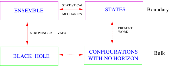
Figure 1: An illustrative description of Mathur’s conjecture. Most of the present research efforts go into improving the dictionary between bulk and boundary microstates (the dotted arrow), and into constructing more microstate geometries.

An analogy that is useful in understanding this proposal is to think about the air in a room. One can use thermodynamics and fluid mechanics to describe the air as a continuous fluid with a certain equation of state. One can also describe the air using statistical mechanics, by finding the typical configurations of molecules in the ensemble, and noticing that the macroscopic features of these configurations are the same as the ones found in the thermodynamic description. For most practical purposes the thermodynamic description is the one to use; however, this description fails to capture the physics coming from the molecular structure of the air. To address problems like Brownian motion, one should not use the thermodynamic approximation, but the statistical description. Similarly, to address questions having to do with physics at the scale of the horizon (like the information paradox) one should not use the thermodynamic approximation, given by the black hole solution, but one should use the statistical description, given by the microstate configurations.

This dramatic shift in the description of black holes, has been most articulately proposed and strongly advocated by Mathur, and is thus often referred to as “Mathur’s conjecture.” In fact, one should be careful and distinguish two variants of this conjecture. The weak variant is that the black hole microstates are horizon-sized stringy configurations that have unitary scattering, but cannot be described accurately using the supergravity approximation. These configurations are also sometimes called “fuzzballs.” If the weak Mathur conjecture were true then the typical bulk microstates would be configurations where the curvature is Planck scale, and hence cannot be described in supergravity. The strong form of Mathur’s conjecture, which is better defined and easier to prove or disprove, is that among the typical black hole microstates there are smooth solutions that can be described using supergravity.

Of course, the configurations that will be discussed and constructed in these notes are classical geometries with a moduli space. Classically, there is an infinite number of such configurations, that need to be quantized before one can call them microstates in the strictest sense of the word. In the analogy with the air in a room, these geometries correspond to classical configurations of molecules. Classically there is an infinite number of such configurations, but one can quantize them and count them to find the entropy of the system.

Whichever version of the conjecture is correct, we are looking for stringy configurations that are very similar to the black hole from far away, and start differing from each other at the location of the would-be horizon. Thus black hole microstates should have a size of the same order as the horizon of the corresponding black hole. From the perspective of string theory, this is very a peculiar feature, since most of the objects that one is familiar with become smaller, not larger, as gravity becomes stronger. We will see in these lectures how our black hole microstates manage to achieve this feature.

If the strong form of this conjecture were true then it would not only solve Hawking’s information paradox (microstates have no horizon, and scattering is unitary), but also would have important consequences for quantum gravity. It also might allow one to derive ’t Hooft’s holographic principle from string theory, and might even have experimental consequences. A more detailed discussion about this can be found in Section 9.

1.3 Outline

As with the two-charge systems, the first step in finding three-charge solutions that have no horizon and look like a black hole is to try to construct large numbers of microscopic stringy three-charge configurations. This is the subject of Section 2, in which we review the construction of three-charge supertubes – string theory objects that have the same charges and supersymmetries as the three-charge black hole [19].

In Section 3 we present the construction of three-charge supergravity solutions corresponding to arbitrary superpositions of black holes, black rings, and three-charge supertubes of arbitrary shape. We construct explicitly a solution corresponding to a black hole at the center of a black ring, and analyze the properties of this solution. This construction and the material presented in subsequent sections can be read independently of Section 2.

Section 4 is a geometric interlude, devoted to Gibbons-Hawking metrics and the relationship between five-dimensional black rings and four-dimensional black holes. Section 5 contains the details of how to construct new microstate solutions using an “ambipolar” Gibbons-Hawking space, whose signature alternates from $(+,+,+,+)$ to $(-,-,-,-)$. Even though the sign of the base-space metric can flip, the full eleven-dimensional solutions are smooth.

In Section 6 we discuss geometric transitions, and the way to obtain smooth horizonless “bubbling” supergravity solutions that have the same type of charges and angular momenta as three-charge black holes and black rings. In Section 7 we construct several such solutions, finding in particular microstates corresponding to zero-entropy black holes and black rings.

In Section 8 we use mergers to construct and analyze “deep microstates,” which correspond to black holes with a classically large horizon area. We find that the depth of these microstates becomes infinite in the classical (large charge) limit, and argue that they correspond to CFT states that have one long component string. This is an essential (though not sufficient) feature of the duals of typical black-hole microstates (for reviews of this, see [20, 21]). Thus the “deep microstates” are either typical microstates themselves, or at least lie in the same sector of the CFT as the typical microstates.

Finally, Section 9 contains conclusions and an extensive discussion of the implications of the work presented here on for the physics of black holes in string theory.

Before beginning we should emphasize that the work that we present is part of a larger effort to study black holes and their microstates in string theory. Many groups have worked at obtaining smooth microstate solutions corresponding to five-dimensional and four-dimensional black holes, a few of the relevant references include [22, 23, 24, 25, 26, 27, 28, 29, 30, 31, 32, 33, 34, 35, 36]. Other groups focus on improving the dictionary between bulk microstates and their boundary counterparts, both in the two-charge and in the three-charge systems [8, 37, 10]. Other groups focus on small black holes and study their properties using the attractor mechanism [39], or relating them to topological strings via the OSV conjecture [40]. Reviews of this can be found in [41], and a limited sample of work that is related to the exploration presented here can be found in [42].

2 Three-charge microscopic configurations

Our purpose here is to follow the historical path taken with the two-charge system and try to construct three-charge brane configurations using the Born-Infeld (BI) action. We are thus considering the intrinsic action of a brane and we will not consider the back-reaction of the brane on the geometry. The complete supergravity solutions will be considered later.

There are several ideas in the study of D-branes that will be important here. First, one of the easiest ways to create system with multiple, different brane charges is to start with a higher-dimensional brane and then turn on electromagnetic fields on that brane so as to induce lower-dimensional branes that are “dissolved” in the original brane. We will use this technique to get systems with D0-D2-D4-D6 charges below.

In constructing multi-charge solutions, one should also remember that the equations of motion are generically non-linear. For example, in supergravity the Maxwell action can involve Chern-Simons terms, or the natural field strength may involve wedge products of lower degree forms. Similarly, in the BI action there is a highly non-trivial interweaving of the Maxwell fields and hence of the brane charges. In practice, this often means that one cannot simply lay down independent charges: Combinations of fields sourced by various charges may themselves source other fields and thus create a distribution of new charges. In this process it is important to keep track of asymptotic charges, which can be measured by the leading fall-off behaviour at infinity, and “dipole” distributions that contribute no net charge when measured at infinity. When one discusses an $N$-charge system one means a system with $N$ commuting asymptotic charges, as measured at infinity. For microstate configurations, one often finds that the systems that have certain charges will also have fields sourced by other dipole charges. More precisely, in discussing the BI action of supertubes we will typically find that a given pair of asymptotic charges, $A$ and $B$, comes naturally with a third set of dipole charges, $C$. We will therefore denote this configuration by $A$-$B$ $\rightarrow$ $C$.

2.1 Three-charge supertubes

The original two-charge supertube [14] carried two independent asymptotic charges, D0 and F1, as well as a D2-brane dipole moment; thus we denote it as a F1-D0 $\rightarrow$ D2 supertube. It is perhaps most natural to try to generalize this object by combining it with another set of branes to provide the third charge. Supersymmetry requires that this new set be D4 branes. To be more precise, supertubes have the same sypersymmetries as the branes whose asymptotic charges they carry and so one can naturally try to put together F1-D0 $\rightarrow$ D2 supertubes, F1-D4 $\rightarrow$ D6 supertubes, and D0-D4 $\rightarrow$ NS5 supertubes, and obtain a supersymmetric configuration that has three asymptotic charges: D0, D4 and F1, and three dipole distributions, coming from D6, NS5 and D2 branes wrapping closed curves. Of course, the intuition coming from putting two-charge supertubes together, though providing useful guidance, will not be able to indicate anything about the size or other properties of the resulting three-charge configuration.

Exercise:  Show that the supertube with D2 dipole charge and F1 and D0 charges can be dualized into an F1-D4 $\rightarrow$ D6 supertube, and into a D0-D4 $\rightarrow$ NS5 supertube.

To investigate objects with the foregoing charges and dipole charges one has to use the theory on one of the sets of branes, and then describe all the other branes as objects in this theory. One route is to consider tubular D6-branes, and attempt to turn on world-volume fluxes to induce D4, D0 and F1 charges. As we will see, such a configuration also has a D2 dipole moment. An alternative route is to use the D4 brane non-Abelian Born-Infeld action. Both routes were pursued in [19], leading to identical results. Nevertheless, for simplicity we will only present the first approach here.

One of the difficulties in describing three-charge supertubes in this way is the fact that the Born-Infeld action and its non-Abelian generalization cannot be used to describe NS5 brane dipole moments. This is essentially because the NS5 brane is a non-perturbative object from the perspective of the Born-Infeld action [90]. Thus, our analysis of three charge supertubes is limited to supertubes that only have D2 and D6 dipole charge. Of course, one can dualize these to supertubes with NS5 and D6 dipole charges, or to supertubes with NS5 and D2. Nevertheless, using the action of a single brane it is not possible to describe supertubes that have three charges and three dipole charges. For that, we will have to wait until Section 3, where we will construct the full supergravity solution corresponding to these objects.

2.2 The Born-Infeld construction

We start with a single tubular D6-brane, and attempt to turn on worldvolume fluxes so that we describe a BPS configuration carrying D4, D0 and F1 charges. We will see that this also necessarily leads to the presence of D2-brane charges, but we will subsequently introduce a second D6-brane to cancel this.

The D6-brane is described by the Born-Infeld action

$${S=-T_{6}\int\!d^{7}\xi~{}\sqrt{-\det(g_{ab}+{\cal F}_{ab})},}$$ (2)

where $g_{ab}$ is the induced worldvolume metric, ${\cal F}_{ab}=2\pi F_{ab}$, $T_{6}$ is the D6-brane tension and we have set $\alpha^{\prime}=1$. The D6 brane also couples to the background RR fields through the Chern-Simons action:

$${S_{CS}=T_{6}\,\int~{}\exp\big{(}{\cal F}+B\big{)}\,\wedge\,\sum_{q}\,C^{(q)}\,.}$$ (3)

By varying this with respect to the $C^{(q)}$ one obtains the D4-brane, D2-brane and D0-brane charge densities:

$$Q_{4} = 2\pi\,T_{6}\,{\cal F}$$ (4)

$$Q_{2} = 2\pi\,T_{6}\,\big{(}{\textstyle{1\over 2}}\displaystyle\,{\cal F}\wedge{\cal F}\big{)}$$ (5)

$$Q_{0} = 2\pi\,T_{6}\,\big{(}{\textstyle{1\over 3!}}\displaystyle\,{\cal F}\wedge{\cal F}\wedge{\cal F}\big{)}\,.$$ (6)

To obtain the quantized Dp-brane charges, one takes the volume $p$-form on any compact, $p$-dimensional spatial region, $R$, and wedges this volume form with $Q_{p}$ and integrates over the spatial section of the D6 brane. The result is then the Dp-brane charge in the region $R$.

The F1 charge density can be obtained by varying the action with respect to the time-space component of NS-NS two form potential, $B$. Since $B$ appears in the combination ${\cal F}+B$, one can differentiate with respect to the gauge field:

$${Q_{1}~{}=~{}{\partial{\cal L}\over\partial B_{0i}}~{}=~{}{\partial{\cal L}\over\partial F_{0i}}~{}=~{}{\partial{\cal L}\over\partial\dot{\vec{A}}}~{}=~{}\vec{\pi}\,,}$$ (7)

which is proportional to the canonical momentum conjugate to the vector potential, $\vec{A}$.

Our construction will essentially follow that of the original D2-brane supertube [14], except that we include four extra spatial dimensions and corresponding fluxes. We take our D6-brane to have the geometry ${R}^{1,1}\times S^{1}\times T^{4}$ and we choose coordinates $(x^{0},x^{1})$ to span ${R}^{1,1}$ and $(x^{6},x^{7},x^{8},x^{9})$ to span the $T^{4}$. The $S^{1}$ will be a circle of of radius $r$ in the $(x^{2},x^{3})$ plane and we will let $\theta$ be the angular coordinate in this plane. We have also introduced factors of $2\pi$ in (4), (5), (6), (7) to anticipate the fact that for round tubes everything will be independent of $\theta$ and so the integrals over $\theta$ will generate these factors of $2\pi$. Thus the D-brane charge densities above are really charge densities in the remaining five dimensions, and the fundamental string charge is a charge density per unit four-dimensional area. Note also that the charges, $Q$, are the ones that appear in the Hamiltonian, and are related to the number of strings or branes by the corresponding tensions. These conventions will be convenient later on.

Since the $S^{1}$ is contractible and lies in the non-compact space-time, any D-brane wrapping this circle will not give rise to asymptotic charges and will only be dipolar. In particular, the configuration carries no asymptotic D6-brane charge due to its tubular shape. To induce D0-branes we turn on constant values of ${\cal F}_{1\theta}$, ${\cal F}_{67},$ and ${\cal F}_{89}$. Turning on ${\cal F}_{1\theta}$ induces a density of D4-branes in the $(x^{6},x^{7},x^{8},x^{9})$ plane, and since these D4 branes only wrap the $T^{4}$, their charge can be measured asymptotically. The fields ${\cal F}_{67},$ and ${\cal F}_{89}$ similarly generate dipolar D4-brane charges. To induce F1 charge in the $x^{1}$ direction we turn on a constant value of ${\cal F}_{01}$. It is also evident from (5) that this configuration carries asymptotic D2-brane charges in the $(x^{6},x^{7})$ and $(x^{8},x^{9})$ planes and dipolar D2-brane charge in the $(x^{1},\theta)$ direction. The asymptotic $D2$-brane charges will eventually be canceled by introducing a second D6-brane. This will also cancel the dipolar D4-brane and D2-brane charges and we will then have a system with asymptotic F1, D0 and D4 charges and dipolar D2 and D6 charges.

With these fluxes turned on we find

$$S=-T_{6}\int\!d^{7}\xi~{}\sqrt{(1-{\cal F}_{01}^{2})r^{2}+{\cal F}_{1\theta}^{2}}\sqrt{(1+{\cal F}_{67}^{2})(1+{\cal F}_{89}^{2})}\,,$$ (8)

where we use polar coordinates in the $(x^{2},x^{3})$ plane, and the factors of $r^{2}$ come from $g_{\theta\theta}$. By differentiating with respect to ${\cal F}_{01}$ we find

$$Q_{1}=2\pi T_{6}{{\cal F}_{01}r^{2}\over\sqrt{(1-{\cal F}_{01}^{2})r^{2}+{\cal F}_{1\theta}^{2}}}\sqrt{(1+{\cal F}_{67}^{2})(1+{\cal F}_{89}^{2})}.$$ (9)

The key point to observe now is that if we choose

$${\cal F}_{01}=1$$ (10)

then $r^{2}$ drops out of the action (8). We will also choose

$${\cal F}_{67}={\cal F}_{89}\,.$$ (11)

We can then obtain the energy from the canonical Hamiltonian:

$$H = \int\!Q_{1}{\cal F}_{01}-L$$ (12)

$$= \int\!\Big{[}Q_{1}+2\pi T_{6}|{\cal F}_{1\theta}|+2\pi T_{6}|{\cal F}_{1\theta}{\cal F}_{67}{\cal F}_{89}|\Big{]}$$ (13)

$$= \int\!\left[Q_{1}+Q_{4}+Q_{0}\right].$$ (14)

The last two integrals are taken over the coordinates $(x^{1},x^{6},x^{7},x^{8},x^{9})$ of the D6-brane. The radius of the system is determined by inverting (9):

$$r^{2}={Q_{1}\over 2\pi T_{6}}{{\cal F}_{1\theta}\over 1+{\cal F}_{67}{\cal F}_{89}}={1\over(2\pi T_{6})^{2}}{Q_{1}Q_{4}^{2}\over Q_{0}+Q_{4}}.$$ (15)

If we set $Q_{0}=0$ then (15) reduces (with the obvious relabeling) to the radius formula found for the original D2-brane supertube [14]. From (14) we see that we have saturated the BPS bound, and so our configuration must solve the equations of motion, as can be verified directly.

Exercise:  Minimize the Hamiltonian in (12) by varying the radius, $r$, while keeping the F1, D0 and D4 charges constant. Verify that the configuration with the radius given (15) solves the equations of motion.

Supersymmetry can also be verified precisely as for the original D2-brane supertube [14]. The presence of the electric field, ${\cal F}_{01}=1$, causes the D6-brane to drop out of the equations determining the tension and the unbroken supersymmetry. Indeed, just like the two-charge system [15], we can consider a D6-brane that wraps an arbitrary closed curve in ${R}^{4}$; the only change in (8) and (9) is that $r^{2}$ will be replace by the induced metric on the D6 brane, $g_{\theta\theta}$. However, when ${\cal F}_{01}=1$ this does not affect equations (13) and (14), and therefore the configuration is still BPS. Moreover, if ${\cal F}_{1\theta}$ is not constant along the tube, or if ${\cal F}_{67}$ and ${\cal F}_{89}$ remain equal but depend on $\theta$ the BPS bound is still saturated.

Hence, classically, there exists an infinite number of three-charge supertubes with two dipole charges, parameterized by several arbitrary functions of one variable [19]. Four of these functions come from the possible shapes of the supertube, and two functions comes from the possibility of varying the D4 and D0 brane densities inside the tube. Anticipating the supergravity results, we expect three-charge, three-dipole charge tubes to be given by seven arbitrary functions, four coming from the shape and three from the possible brane densities inside the tube. The procedure of constructing supergravity solutions corresponding to these objects [44, 45] will be discussed in the next section, and will make this “functional freedom” very clear.

As we have already noted, the foregoing configuration also carries non-vanishing D2-brane charge associated with ${\cal F}_{1\theta}{\cal F}_{67}$ and ${\cal F}_{1\theta}{\cal F}_{89}$. It also carries dipolar D4-brane charges associated with ${\cal F}_{67}$ and ${\cal F}_{89}$. To remedy this we can introduce one more D6 brane with flipped signs of ${\cal F}_{67}$ and ${\cal F}_{89}$ [47]. This simply doubles the D4, D0, and F1 charges, while canceling the asymptotic D2 charge and the dipolar D4-brane charges. More generally, we can introduce $k$ coincident D6-branes, with fluxes described by diagonal $k\times k$ matrices. We again take the matrix-valued field strengths ${\cal F}_{01}$ to be equal to the unit matrix, in order to obtain a BPS state. We also set ${\cal F}_{67}={\cal F}_{89}$, and take $F_{1\theta}$ to have non-negative diagonal entries to preclude the appearance of $\overline{D4}$-branes. The condition of vanishing D2-brane charge is then

$${\rm Tr}~{}{\cal F}_{1\theta}~{}{\cal F}_{67}~{}=~{}{\rm Tr}~{}{\cal F}_{1\theta}{\cal F}_{89}~{}=~{}0.$$ (16)

This configuration can also have D4-brane dipole charges, which we may set to zero by choosing

$${\rm Tr}~{}{\cal F}_{67}~{}=~{}{\rm Tr}~{}{\cal F}_{89}~{}=~{}0.$$ (17)

Finally, the F1 charge is described by taking $Q_{1}$ to be an arbitrary diagonal matrix with non-negative entries. This results in a BPS configuration of $k$ D6-branes wrapping curves of arbitrary shape. If the curves are circular, the radius formula is now given by (15) but with the entries replaced by the corresponding matrices. Of course, for our purposes we are interested in situations when we can use the Born-Infeld action of the D6 branes to describe the dynamics of our objects. Since the BI action does not take into account interactions between separated strands of branes, we will henceforth restrict ourselves to the situations where these curves are coincident. In analogy with the behaviour of other branes, if we take the $k$ D6-branes to sit on top of each other we expect that they can form a marginally bound state. In the classical description we should then demand that the radius matrix (15) be proportional to the unit matrix. Given a choice of magnetic fluxes, this determines the F1 charge matrix $Q_{1}$ up to an overall multiplicative constant that parameterizes the radius of the combined system.

Since our matrices are all diagonal, the Born-Infeld action is unchanged except for the inclusion of an overall trace. Similarly, the energy is still given by $H=\int\!{\rm Tr}\left[Q_{1}+Q_{4}+Q_{0}\right]$.

Consider the example in which all $k$ D6-branes are identical modulo the sign of ${\cal F}_{67}$ and ${\cal F}_{89}$, so that both ${\cal F}_{1\theta}$ and ${\cal F}_{67}{\cal F}_{89}$ are proportional to the unit matrix. Then, in terms of the total charges, the radius formula is

$$r^{2}~{}=~{}{1\over k^{2}(2\pi T_{6})^{2}}{Q_{1}^{\rm tot}(Q_{4}^{\rm tot})^{2}\over Q_{0}^{\rm tot}+Q_{4}^{\rm tot}}\,.$$ (18)

Observe that after fixing the conserved charges and imposing equal radii for the component tubes, there is still freedom in the values of the fluxes. These can be partially parameterized in terms of various non-conserved “charges”, such as brane dipole moments. Due to the tubular configuration, our solution carries non-zero D6, D4, and D2 dipole moments, proportional to

$$Q^{D}_{6} = T_{6}\,r\,k$$

$$Q^{D}_{4} = T_{6}\,r\,{\rm Tr}\,{\cal F}_{67}$$

$$Q^{D}_{2} = T_{6}\,r\,{\rm Tr}\,{\cal F}_{67}\,{\cal F}_{89}\equiv T_{6}\,r\,k_{2}.$$ (19)

When the $k$ D6-branes that form the tube are coincident, $k_{2}$ measures the local D2 brane dipole charge of the tube. It is also possible to see that both for a single tube, and for $k$ tubes identical up to the sign of ${\cal F}_{67}$ and ${\cal F}_{89}$, the dipole moments are related via:

$${Q_{2}^{D}\over Q_{6}^{D}}~{}=~{}{k_{2}\over k}~{}=~{}{Q^{\rm tot}_{0}\over Q^{\rm tot}_{4}}\,.$$ (20)

We will henceforth drop the superscripts on the $Q^{\rm tot}_{p}$ and denote them by $Q_{p}$. One can also derive the microscopic relation, (20), from the supergravity solutions that we construct in Section 3.4. In the supergravity solution one has to set one of the three dipole charges to zero to obtain the solution with three asymptotic charges and two dipole charges. One then finds that (20) emerges from are careful examination of the near-horizon limit and the requirement that the solution be free of closed timelike curves [46].

If ${\cal F}_{67}$ and ${\cal F}_{89}$ are traceless, this tube has no D2 charge and no D4 dipole moment. More general tubes will not satisfy (20), and need not have vanishing D4 dipole moment when the D2 charge vanishes. We should also remark that the D2 dipole moment is an essential ingredient in constructing a supersymmetric three-charge tube of finite size. When this dipole moment goes to zero, the radius of the tube also becomes zero.

In general, we can construct a tube of arbitrary shape, and this tube will generically carry angular momentum in the $(x^{2},x^{3})$ and $(x^{4},x^{5})$ planes. We can also consider a round tube, made of $k$ identical D6 branes wrapping an $S^{1}$ that lies for example in the $(x^{2},x^{3})$ plane. The microscopic angular momentum density of such a configuration is given by the $(0,\theta)$ component of the energy-momentum tensor:

$$J_{23}~{}=~{}2\pi\,r\,T_{0\theta}~{}=~{}2\pi T_{6}\,k\,r^{2}\,\sqrt{(1+{\cal F}_{67}^{2})(1+{\cal F}_{89}^{2})}\,.$$ (21)

Now recall that supersymmetry requires ${\cal F}_{67}={\cal F}_{89}$ and that ${\rm Tr}({\cal F}_{67}{\cal F}_{89})=Q_{0}/Q_{4}$ and so this may be rewritten as:

$$J_{23}~{}=~{}2\pi T_{6}\,k\,r^{2}\,\Big{(}1~{}+~{}{Q_{0}\over Q_{4}}\Big{)}~{}=~{}{1\over 2\pi T_{6}}\,{Q_{1}\,Q_{4}\over k}\,,$$ (22)

where we have used (18). It is interesting to note that this microscopic angular momentum density is not necessarily equal to the angular momentum measured at infinity. As we will see in the next section from the full supergravity solution, the angular momenta of the three-charge supertube also have a piece coming from the supergravity fluxes. This is similar to the non-zero angular momentum coming from the Poynting vector, $\vec{E}\times\vec{B}$, in the static electromagnetic configuration consisting of an electron and a magnetic monopole [48].

Note also that when one adds D0 brane charge to a F1-D4 supertube, the angular momentum does not change, even if the radius becomes smaller. Hence, given charges of the same order, the angular momentum that the ring carries is of order the square of the charge (for a fixed number, $k$, of $D6$ branes). For more general three-charge supertubes, whose shape is an arbitrary curve inside ${R}^{4}$, the angular momenta can be obtained rather straightforwardly from this shape by integrating the appropriate components of the BI energy-momentum tensor over the profile of the tube.

A T-duality along $x^{1}$ transforms our D0-D4-F1 tubes into the more familiar D1-D5-P configurations. This T-duality is implemented by the replacement $2\pi A^{1}\rightarrow X^{1}$. The non-zero value of ${\cal F}_{1\theta}$ is translated by the T-duality into a non-zero value of $\partial_{\theta}X^{1}$. This means that the resulting D5-brane is in the shape of a helix whose axis is parallel to $x^{1}$. This is the same as the observation that the D2-brane supertube T-dualizes into a helical D1-brane. Since this helical shape is slightly less convenient to work with than a tube, we have chosen to emphasize the F1-D4-D0 description instead. Nevertheless, in the formulas that give the radius and angular momenta of the three-charge supertubes we will use interchangingly the D1-D5-P and the D0-D4-F1 quantities, related via U-duality $N_{0}\rightarrow N_{p}$, $N_{4}\rightarrow N_{5}$, and $N_{1}\rightarrow N_{1}$, with similar replacements for the $Q$’s.

Exercise:  Write the combination of S-duality and T-duality transformations that corresponds to this identification of the D1-D5-P and F1-D4-D0 quantities.

2.3 Supertubes and black holes

The spinning three-charge black hole (also known as the BMPV black hole [49]) can only carry equal angular momenta, bounded above by:

$$J_{1}^{2}~{}=~{}J_{2}^{2}~{}\leq~{}N_{1}N_{5}N_{P}\,.$$ (23)

For the three-charge supertubes, the angular momenta are not restricted to be equal. A supertube configuration can have arbitrary shape, and carry any combination of the two angular momenta. For example, we can choose a closed curve such that the supertube cross-section lies in the $(x^{2},x^{3})$ plane, for which $J_{23}\neq 0$ and $J_{45}=0$. The bound on the angular momentum can be obtained from (22):

$$|J|~{}=~{}{1\over 2\pi T_{6}}\,{Q_{1}\,Q_{4}\over k}~{}\leq~{}{1\over 2\pi T_{6}}\,{Q_{1}\,Q_{4}}~{}=~{}N_{1}\,N_{4}\,,$$ (24)

where we have used $k\geq 1$ since it is the number of D6 branes. The quantized charges are given by $Q_{1}={1\over 2\pi}N_{1}$, $Q_{4}=(2\pi)^{2}T_{6}N_{4}$. We therefore see that a single D6 brane saturates the bound and that by varying the number of D6 branes or by appropriately changing the shape and orientation of the tube cross section, we can span the entire range of angular momenta between $-N_{1}N_{4}$ and $+N_{1}N_{4}$. Since (24) is quadratic the charges, one can easily exceed the black hole angular momentum bound in (23) by simply making $Q_{1}$ and $Q_{4}$ sufficiently large.

One can also compare the size of the supertube with the size of the black hole. Using (24), one can rewrite (18) in terms of the angular momentum:

$$r^{2}~{}=~{}{J^{2}\over Q_{1}\,(Q_{0}+Q_{4})}\,,$$ (25)

Now recall that the tension of a D-brane varies as $g_{s}^{-1}$ and that the charges, $Q_{0}$ and $Q_{4}$, appear in the Hamiltonian, (14). This means that the quantization conditions on the D-brane charges must have the form $Q_{j}\sim N_{j}/g_{s}$. The energy of the fundamental string is independent of $g_{s}$ and so $Q_{1}\sim N_{1}$, with no factors of $g_{s}$. If we take $N_{0}\approx N_{1}\approx N_{4}\approx N$ then we find:

$$r_{\rm tube}^{2}~{}\sim~{}g_{s}\,{J^{2}\over N^{2}}\,.$$ (26)

From the BMPV black hole metric [49, 50] one can compute the proper length of the circumference of the horizon (as measured at one of the equator circles) to be

$${r_{\rm hole}^{2}~{}\sim~{}g_{s}\,{N^{3}-J^{2}\over N^{2}}~{}.}$$ (27)

The most important aspect of the equations (26) and (27) is that for comparable charges and angular momenta, the black hole and the three-charge supertube have comparable sizes. Moreover, these sizes grow with $g_{s}$ in the same way. This is a very counter-intuitive behavior. Most of the objects we can think about tend to become smaller when gravity is made stronger and this is consistent with our intuition and the fact that gravity is an attractive force. The only “familiar” object that becomes larger with stronger gravity is a black hole. Nevertheless, three-charge supertubes also become larger as gravity becomes stronger! The size of a tube is determined by a balance between the angular momentum of the system and the tension of the tubular brane. As the string coupling is increased, the D-brane tension decreases, and thus the size of the tube grows, at exactly the same rate as the Schwarzschild radius of the black hole.

This is the distinguishing feature that makes the three-charge supertubes (as well as the smooth geometries that we will obtain from their geometric transitions) unlike any other configuration that one counts in studying black hole entropy.

To be more precise, let us consider the counting of states that leads to the black hole entropy “à la Strominger and Vafa.” One counts microscopic brane/string configurations at weak coupling where the system is of string scale in extent, and its Schwarzschild radius even smaller. One then imagines increasing the gravitational coupling; the Schwarzschild radius grows, becoming comparable to the size of the brane configuration at the “correspondence point” [51], and larger thereafter. When the Schwarzschild radius is much larger than the Planck scale, the system can be described as a black hole. There are thus two very different descriptions of the system: as a microscopic string theory object for small $g_{s}$, and as a black hole for large $g_{s}$. One then compares the entropy in the two regimes and finds an agreement, which is precise if supersymmetry forbids corrections during the extrapolation.

Three-charge supertubes behave differently. Their size grows at the same rate as the Schwarzschild radius, and thus they have no “correspondence point.” Their description is valid in the same regime as the description of the black hole. If by counting such configurations one could reproduce the entropy of the black hole, then one should think about the supertubes as the large $g_{s}$ continuation of the microstates counted at small $g_{s}$ in the string/brane picture, and therefore as the microstates of the corresponding black hole.

It is interesting to note that if the supertubes did not grow with exactly the same power of $g_{s}$ as the black hole horizon, they would not be good candidates for being black hole microstates, and Mathur’s conjecture would have been in some trouble. The fact that there exists a huge number of configurations that do have the same growth with $g_{s}$ as the black hole is a non-trivial confirmation that these configurations may well represent black-hole microstates for the three-charge system.

We therefore expect that configurations constructed from three-charge supertubes will give us a large number of three-charge BPS black hole microstates. Nevertheless, we have seen that three-charge supertubes can have angular momenta larger than the BPS black hole, and generically have $J_{1}\neq J_{2}$. Hence one can also ask if there exists a black object whose microstates those supertubes represent. In [19] it was conjectured that such an object should be a three-charge BPS black ring, despite the belief at the time that there was theorem that such BPS black rings could not exist. After more evidence for this conjecture came from the construction of the flat limit of black rings [46], a gap in the proof of the theorem was found [52]. Subsequently the BPS black ring with equal charges and dipole charges was found in [53], followed by the rings with three arbitrary charges and three arbitrary dipole charges [44, 54, 55]. One of the morals of this story is that whenever one encounters an “established” result that contradicts intuition one should really get to the bottom of it and find out why the intuition is wrong or to expose the cracks in established wisdom.

3 Black rings and supertubes

As we have seen in the D-brane analysis of the previous section, three-charge supertubes of arbitrary shape preserve the same supersymmetries as the three-charge black hole. Moreover, as we will see, three-charge supertube solutions that have three dipole charges can also have a horizon at large effective coupling, and thus become black rings. Therefore, one expects the existence of BPS configurations with an arbitrary distribution of black holes, black rings and supertubes of arbitrary shape. Finding the complete supergravity solution for such configurations appears quite daunting. We now show that this is nevertheless possible and that the entire problem can be reduced to solving a linear system of equations in four-dimensional, Euclidean electromagnetism.

3.1 Supersymmetric configurations

We begin by considering brane configurations that preserve the same supersymmetries as the three-charge black hole. In M-theory, the latter can be constructed by compactifying on a six-torus, $T^{6}$, and wrapping three sets of M2 branes on three orthogonal two-tori (see the first three rows of Table 1). Amazingly enough, one can add a further three sets of M5 branes while preserving the same supersymmetries: Each set of M5 branes can be thought of as magnetically dual to a set of M2 branes in that the M5 branes wrap the four-torus, $T^{4}$, orthogonal to the $T^{2}$ wrapped by the M2 branes. The remaining spatial direction of the M5 branes follows a simple, closed curve, $y^{\mu}(\sigma)$, in the spatial section of the five-dimensional space-time. Since we wish to make a single, three-charge ring we take this curve to be the same for all three sets of M5 branes. This configuration is summarized in Table 1. In [44] it was argued that this was the most general three-charge brane configuration consistent with the supersymmetries of the three-charge black-hole.

Brane	0	1	2	3	4	5	6	7	8	9	10
M2	$\updownarrow$	$\star$	$\star$	$\star$	$\star$	$\updownarrow$	$\updownarrow$	$\leftrightarrow$	$\leftrightarrow$	$\leftrightarrow$	$\leftrightarrow$
M2	$\updownarrow$	$\star$	$\star$	$\star$	$\star$	$\leftrightarrow$	$\leftrightarrow$	$\updownarrow$	$\updownarrow$	$\leftrightarrow$	$\leftrightarrow$
M2	$\updownarrow$	$\star$	$\star$	$\star$	$\star$	$\leftrightarrow$	$\leftrightarrow$	$\leftrightarrow$	$\leftrightarrow$	$\updownarrow$	$\updownarrow$
M5	$\updownarrow$	$y^{\mu}(\sigma)$				$\leftrightarrow$	$\leftrightarrow$	$\updownarrow$	$\updownarrow$	$\updownarrow$	$\updownarrow$
M5	$\updownarrow$	$y^{\mu}(\sigma)$				$\updownarrow$	$\updownarrow$	$\leftrightarrow$	$\leftrightarrow$	$\updownarrow$	$\updownarrow$
M5	$\updownarrow$	$y^{\mu}(\sigma)$				$\updownarrow$	$\updownarrow$	$\updownarrow$	$\updownarrow$	$\leftrightarrow$	$\leftrightarrow$

Table 1: Layout of the branes that give the supertubes and black rings in an M-theory duality frame. Vertical arrows $\updownarrow$, indicate the directions along which the branes are extended, and horizontal arrows, $\leftrightarrow$, indicate the smearing directions. The functions, $y^{\mu}(\sigma)$, indicate that the brane wraps a simple closed curve in ${R}^{4}$ that defines the black-ring or supertube profile. A star, $\star$, indicates that a brane is smeared along the supertube profile, and pointlike on the other three directions.

The metric corresponding to this brane configuration can be written as

$$ds_{11}^{2}=ds_{5}^{2} + \left(Z_{2}Z_{3}Z_{1}^{-2}\right)^{1\over 3}(dx_{5}^{2}+dx_{6}^{2})$$ (28)

$$+ \left(Z_{1}Z_{3}Z_{2}^{-2}\right)^{1\over 3}(dx_{7}^{2}+dx_{8}^{2})+\left(Z_{1}Z_{2}Z_{3}^{-2}\right)^{1\over 3}(dx_{9}^{2}+dx_{10}^{2})\,,$$

where the five-dimensional space-time metric has the form:

$$ds_{5}^{2}~{}\equiv~{}-\left(Z_{1}Z_{2}Z_{3}\right)^{-{2\over 3}}(dt+k)^{2}+\left(Z_{1}Z_{2}Z_{3}\right)^{1\over 3}\,h_{\mu\nu}dy^{\mu}dy^{\nu}\,,$$ (29)

for some one-form field, $k$, defined upon the spatial section of this metric. Since we want the metric to be asymptotic to flat ${R}^{4,1}\times T^{6}$, we require

$$ds_{4}^{2}~{}\equiv~{}h_{\mu\nu}dy^{\mu}dy^{\nu}\,,$$ (30)

to limit to the flat, Euclidean metric on ${R}^{4}$ at spatial infinity and we require the warp factors, $Z_{I}$, to limit to constants at infinity. To fix the normalization of the corresponding Kaluza-Klein $U(1)$ gauge fields, we will take $Z_{I}\to 1$ at infinity.

The supersymmetry, $\epsilon$, consistent with the brane configurations in Table 1 must satisfy:

$$\big{(}\hbox to0.0pt{1\hss}\mkern 4.0mu{\rm l}~{}-~{}\Gamma^{056})\,\epsilon~{}=~{}\big{(}\hbox to0.0pt{1\hss}\mkern 4.0mu{\rm l}~{}-~{}\Gamma^{078})\,\epsilon~{}=~{}\big{(}\hbox to0.0pt{1\hss}\mkern 4.0mu{\rm l}~{}-~{}\Gamma^{09\,10})\,\epsilon~{}=~{}0\,.$$ (31)

Since the product of all the gamma-matrices is the identity matrix, this implies

$$\big{(}\hbox to0.0pt{1\hss}\mkern 4.0mu{\rm l}~{}-~{}\Gamma^{1234})\,\epsilon~{}=~{}0\,,$$ (32)

which means that one of the four-dimensional helicity components of the four dimensional supersymmetry must vanish identically. The holonomy of the metric, (30), acting on the spinors is determined by

$$[\,\nabla_{\mu}\,,\,\nabla_{\nu}\,]\,\epsilon~{}=~{}{\textstyle{1\over 4}}\displaystyle\,R^{(4)}_{\mu\nu cd}\,\Gamma^{cd}\,\epsilon\,,$$ (33)

where $R^{(4)}_{\mu\nu cd}$ is the Riemann tensor of (30). Observe that (33) vanishes identically as a consequence of (32) if the Riemann tensor is self-dual:

$$R^{(4)}_{abcd}~{}=~{}{\textstyle{1\over 2}}\displaystyle\,{\varepsilon_{cd}}^{ef}\,R^{(4)}_{abef}\,.$$ (34)

Such four-metrics are called “half-flat.” Equivalently, note that the holonomy of a general Euclidean four-metric is $SU(2)\times SU(2)$ and that (34) implies that the holonomy lies only in one of these $SU(2)$ factors and that the metric is flat in the other factor. The condition (32) means that all the components of the supersymmetry upon which the non-trivial holonomy would act actually vanish. The other helicity components feel no holonomy and so the supersymmetry can be defined globally. One should also note that $SU(2)$ holonomy in four-dimensions is equivalent to requiring that the metric be hyper-Kähler.

Thus we can preserve the supersymmetry if and only if we take the four-metric to be hyper-Kähler. However, there is a theorem that states that any metric that is (i) Riemannian (signature $+4$) and regular, (ii) hyper-Kähler and (iii) asymptotic to the flat metric on ${R}^{4}$, must be globally the flat metric on ${R}^{4}$. The obvious conclusion, which we will follow in this section, is that we simply take (30) to be the flat metric on ${R}^{4}$. However, there are very important exceptions. First, we require the four-metric to be asymptotic to flat ${R}^{4}$ because we want to interpret the object in asymptotically flat, five-dimensional space-time. If we want something that can be interpreted in terms of asymptotically flat, four-dimensional space-time then we want the four-metric to be asymptotic to the flat metric on ${R}^{3}\times S^{1}$. This allows for a lot more possibilities, and includes the multi-Taub-NUT metrics [56]. Using such Taub-NUT metrics provides a straightforward technique for reducing the five-dimensional solutions to four dimensions [27, 57, 58, 59, 60].

The other exception will be the subject of subsequent sections of this review: The requirement that the four-metric be globally Riemannian is too stringent. As we will see, the metric can be allowed to change the overall sign since this can be compensated by a sign change in the warp factors of (29). In this section, however, we will suppose that the four-metric is simply that of flat ${R}^{4}$.

3.2 The BPS equations

The Maxwell three-form potential is given by

$$C^{(3)}=A^{(1)}\wedge dx_{5}\wedge dx_{6}~{}+~{}A^{(2)}\wedge dx_{7}\wedge dx_{8}~{}+~{}A^{(3)}\wedge dx_{9}\wedge dx_{10}\,,$$ (35)

where the six coordinates, $x_{A}$, parameterize the compactification torus, $T^{6}$, and $A^{(I)}$, $I=1,2,3$, are one-form Maxwell potentials in the five-dimensional space-time and depend only upon the coordinates, $y^{\mu}$, that parameterize the spatial directions. It is convenient to introduce the Maxwell “dipole field strengths,” $\Theta^{(I)}$, obtained by removing the contributions of the electrostatic potentials

$$\Theta^{(I)}~{}\equiv~{}dA^{(I)}+d\big{(}Z_{I}^{-1}\,(dt+k)\big{)}\,,$$ (36)

The most general supersymmetric configuration is then obtained by solving the BPS equations:

$$\Theta^{(I)} ~{}=~{} \star_{4}\,\Theta^{(I)}\,,$$ (37)

$$\nabla^{2}Z_{I} ~{}=~{} {1\over 2}C_{IJK}\star_{4}(\Theta^{(J)}\wedge\Theta^{(K)})\,,$$ (38)

$$dk~{}+~{}\star_{4}dk ~{}=~{} Z_{I}\,\Theta^{(I)}\,,$$ (39)

where $\star_{4}$ is the Hodge dual taken with respect to the four-dimensional metric $h_{\mu\nu}$, and structure constants are given by $C_{IJK}~{}\equiv~{}|\epsilon_{IJK}|$. It is important to note that if these equations are solved in the order presented above, then one is solving a linear system.

At each step in the solution-generating process one has the freedom to add homogeneous solutions of the equations. Since we are requiring that the fields fall off at infinity, this means that these homogeneous solutions must have sources in the base space and since there is no topology in the ${R}^{4}$ base, these sources must be singular. One begins by choosing the profiles, in ${R}^{4}$, of the three types of M5 brane that source the $\Theta^{(I)}$. These fluxes then give rise to the explicit sources on the right-hand side of (38), but one also has the freedom to choose singular sources for (38) corresponding to the densities, $\rho_{I}(\sigma)$, of the three types of M2 branes. The M2 branes can be distributed at the same location as the M5 profile, and can also be distributed away from this profile. (See Fig. 2.) The functions, $Z_{I}$, then appear in the final solution as warp factors and as the electrostatic potentials. There are thus two contributions to the total electric charge of the solution: The localized M2 brane sources described by $\rho_{I}(\sigma)$ and the induced charge from the fields, $\Theta^{(I)}$, generated by the M5 branes. It is in this sense that the solution contains electric charges that are dissolved in the fluxes generated by M5 branes, much like in the Klebanov-Strassler or Klebanov-Tseytlin solutions [61, 62].

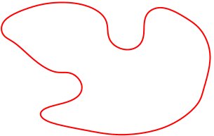
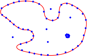
Figure 2: The first two steps of the procedure to construct solutions. One first chooses an arbitrary M5 brane profile, and then sprinkles the various types of M2 branes, either on the M5 brane profile, or away from it. This gives a solution for an arbitrary superposition of black rings, supertubes and black holes.

The final step is to solve the last BPS equation, (39), which is sourced by a cross term between the magnetic and electric fields. Again there are homogeneous solutions that may need to be added and this time; however they need to be adjusted so as to ensure that (29) has no closed time-like curves (CTC’s). Roughly one must make sure that the angular momentum at each point does not exceed what can be supported by local energy density.

3.3 Asymptotic charges

Even though a generic black ring is made from six sets of branes, there are only three conserved electric charges that can be measured from infinity. These are obtained from the three vector potentials, $A^{(I)}$, defined in (35), by integrating $\star_{5}dA^{(I)}$ over the three-sphere at spatial infinity. Since the M5 branes run in a closed loop, they do not directly contribute to the electric charges. The electric charges are determined by electric fields at infinity, and hence by the functions $Z_{I}$ (36). Indeed, one has:

$$Z_{I}~{}\sim~{}1~{}+~{}c_{1}\,{Q_{I}\over\rho^{2}}~{}+~{}\dots\,,\qquad\rho\to\infty\,,$$ (40)

where $c_{1}$ is a normalization constant (discussed below), $\rho$ is the standard, Euclidean radial coordinate in ${R}^{4}$ and the $Q_{I}$ are the electric charges. Note that while the M5 branes do not directly contribute to the electric charges, they do contribute indirectly via “charges dissolved in fluxes,” that is, through the source terms on the right-hand side of (38).

To compute the angular momentum it is convenient to write the spatial ${R}^{4}$ as ${R}^{2}\times{R}^{2}$ and pass to two sets of polar coordinates, $(u,\theta_{1})$ and $(v,\theta_{2})$ in which the flat metric on ${R}^{4}$ is:

$$ds_{4}^{2}~{}=~{}(du^{2}~{}+~{}u^{2}\,d\theta_{1}^{2})~{}+~{}(dv^{2}~{}+~{}v^{2}\,d\theta_{2}^{2})\,.$$ (41)

There are two commuting angular momenta, $J_{1}$ and $J_{2}$, corresponding to the components of rotation in these two planes. One can then read off the angular momentum by making an expansion at infinity of the angular momentum vector, $k$, in (29):

$$k~{}\sim~{}c_{2}\,\bigg{(}J_{1}\,{u^{2}\over(u^{2}+v^{2})^{2}}~{}+~{}J_{2}\,{v^{2}\over(u^{2}+v^{2})^{2}}\bigg{)}~{}+~{}\dots~{}\,,\qquad u,v\to\infty\,,$$ (42)

where $c_{2}$ is a normalization constant. The charges, $Q_{I}$, and the angular momenta, $J_{1},J_{2}$, need to be correctly normalized in order to express them in terms of the quantized charges. The normalization depends upon the eleven-dimensional Planck length, $\ell_{p}$, and the volume of the compactifying torus, $T^{6}$. The correct normalization can be found [44], and has been computed in many references. (For a good review, see [63].) Here we simply state that if $L$ denotes the radius of the circles that make up the $T^{6}$ (so that the compactification volume is $V_{6}=(2\pi L)^{6}$), then one obtains the canonically normalized quantities by using

$$c_{1}~{}=~{}{\ell_{p}^{6}\over L^{4}}\,,\qquad c_{2}~{}=~{}{\ell_{p}^{9}\over L^{6}}\,.$$ (43)

For simplicity, in most of the rest of this review we will take as system of units in which $\ell_{p}=1$ and we will fix the torus volume so that $L=1$. Thus one has $c_{1}=c_{2}=1$.

3.4 An example: A three-charge black ring with a black hole in the middle

By solving the BPS equations, (37)–(39), one can, in principle, find the supergravity solution for an arbitrary distribution of black rings and black holes. The metric for a general distribution of these objects will be extremely complicated, and so to illustrate the technique we will concentrate on a simpler system: A BMPV black hole at the center of a three-charge BPS black ring. An extensive review of black rings, both BPS and non-BPS can be found in [64]. Other interesting papers related to non-BPS black rings include [65].

Since the ring sits in an ${R}^{2}$ inside ${R}^{4}$, it is it is natural to pass to the two sets of polar coordinates, $(u,\theta_{1})$ and $(v,\theta_{2})$ in which the base-space metric takes the form (41) We then locate the ring at $u=R$ and $v=0$ and the black hole at $u=v=0$.

The best coordinate system for actually solving the black ring equations is the one that has become relatively standard in the black-ring literature (see, for example, [53]). The change of variables is:

$$x ~{}=~{} -{u^{2}+v^{2}-R^{2}\over\sqrt{((u-R)^{2}+v^{2})((u+R)^{2}+v^{2})}}\,,$$ (44)

$$y ~{}=~{} -{u^{2}+v^{2}+R^{2}\over\sqrt{((u-R)^{2}+v^{2})((u+R)^{2}+v^{2})}}\,,$$ (45)

where $-1\leq x\leq 1$, $-\infty<y\leq-1$, and the ring is located at $y=-\infty$. This system has several advantages: it makes the electric and magnetic two-form field strengths sourced by the ring have a very simple form (see (47)), and it makes the ring look like a single point while maintaining separability of the Laplace equation. In these coordinates the flat ${R}^{4}$ metric has the form:

$$ds_{4}^{2}~{}=~{}{R^{2}\over(x-y)^{2}}\left({dy^{2}\over y^{2}-1}+(y^{2}-1)d\theta_{1}^{2}+{dx^{2}\over 1-x^{2}}+(1-x^{2})d\theta_{2}^{2}\right).$$ (46)

The self-dual field strengths that are sourced by the ring are then:

$$\Theta^{(I)}~{}=~{}2\,q_{i}\,(dx\wedge d\theta_{2}~{}-~{}dy\wedge d\theta_{1})\,.$$ (47)

The warp factors then have the form

$$Z_{I}~{}=~{}1~{}+~{}{\overline{Q}_{I}\over R}(x-y)~{}-~{}{2\,C_{IJK}\,q^{J}q^{K}\over R^{2}}\,(x^{2}-y^{2})~{}-~{}{Y_{I}\over R^{2}}\,{x-y\over x+y}\,,$$ (48)

and the angular momentum components are given by:

$$k_{\psi} = (y^{2}-1)\,g(x,y)-\,A\,(y+1)\,,\qquad k_{\phi}=(x^{2}-1)\,g(x,y)\,;$$ (49)

$$g(x,y) \equiv \left({C\over 3}\,(x+y)~{}+~{}{B\over 2}-{D\over R^{2}(x+y)}+{K\over R^{2}(x+y)^{2}}\right)$$ (50)

where $K$ represents the angular momentum of the BMPV black hole and

$$A ~{}\equiv~{} 2\big{(}\sum q^{I}\big{)}\,,\qquad\qquad B~{}\equiv~{}{2\over R}\,(Q_{I}q^{I})\,,\qquad$$ (51)

$$C ~{}\equiv~{} -{8\,C_{IJK}\,q^{I}q^{J}q^{K}\over R^{2}}\,,\qquad D~{}\equiv~{}{2}\,Y_{I}q^{I}\,.$$ (52)

The homogeneous solutions of (39) have already been chosen so as to remove any closed timelike curves (CTC).

The relation between the quantized ring and black-hole charges and the parameters appearing in the solution are:

$$\overline{Q}_{I}={\overline{N}_{I}\,\ell_{p}^{6}\over 2L^{4}R}\,,\qquad q^{I}={n^{I}\,\ell_{p}^{3}\over 4L^{2}}\,,\qquad Y_{I}={N^{\rm BH}_{I}\,\ell_{p}^{6}\over L^{4}}\,,\qquad K={J^{\rm BMPV}\,\ell_{p}^{9}\over L^{6}}\,,$$ (53)

where $L$ is the radius of the circles that make up the $T^{6}$ (so that $V_{6}=(2\pi L)^{6}$) and $\ell_{p}$ is the eleven-dimensional Planck length.

As we indicated earlier, the asymptotic charges, $N_{I}$, of the solution are the sum of the microscopic charges on the black ring, $\overline{N}_{I}$, the charges of the black hole, $N^{\rm BH}_{I}$, and the charges dissolved in fluxes:

$$N_{I}~{}=~{}\overline{N}_{I}~{}+~{}N^{\rm BH}_{I}~{}+~{}{\textstyle{1\over 2}}\displaystyle\,C_{IJK}\,n^{J}n^{K}\,.$$ (54)

Exercise:  Derive this expression for the charge from the asymptotic expansion of the $Z_{I}$ in (48). Derive the relation between the parameters $q^{I}$ and the quantized M5 charges $n^{I}$ in (53), by integrating the magnetic M-theory four-form field strength around the ring profile. (See, for example, [63] in order to get the charge normalizations precisely correct.)

The angular momenta of this solution are:

$$J_{1} = J_{\Delta}~{}+~{}\Big{(}{\textstyle{1\over 6}}\displaystyle\,C_{IJK}\,n^{I}n^{J}n^{K}~{}+~{}{\textstyle{1\over 2}}\displaystyle\,\overline{N}_{I}n^{I}~{}+~{}N^{\rm BH}_{I}n^{I}~{}+~{}J^{\rm BMPV}\Big{)}\,,$$ (55)

$$J_{2} = -\Big{(}{\textstyle{1\over 6}}\displaystyle\,C_{IJK}\,n^{I}n^{J}n^{K}~{}+~{}{\textstyle{1\over 2}}\displaystyle\,\overline{N}_{I}n^{I}~{}+~{}N^{\rm BH}_{I}n^{I}~{}+~{}J^{\rm BMPV}\Big{)}\,,$$ (56)

where

$$J_{\Delta}~{}\equiv~{}{R^{2}L^{4}\over l_{p}^{6}}\,\Big{(}\sum n^{I}\Big{)}\,.$$ (57)

The entropy of the ring is:

$$S~{}=~{}{2\pi A\over\kappa_{11}^{2}}~{}=~{}\pi\,\sqrt{\cal M}$$ (58)

where

$${\cal M} ~{}\equiv~{} 2\,n^{1}n^{2}\overline{N}_{1}\overline{N}_{2}+2\,n^{1}n^{3}\overline{N}_{1}\overline{N}_{3}+2\,n^{2}n^{3}\overline{N}_{2}\overline{N}_{3}-(n^{1}\overline{N}_{1})^{2}$$ (59)

$$\quad-(n^{2}\overline{N}_{2})^{2}-(n^{3}\overline{N}_{3})^{2}-4\,n^{1}n^{2}n^{3}\,J_{T}\,.$$

and

$$J_{T}~{}\equiv~{}J_{\Delta}+n^{I}N^{\rm BH}_{I}~{}=~{}{R^{2}L^{4}\over l_{p}^{6}}\,\Big{(}\sum n^{I}\Big{)}~{}+~{}n^{I}N^{\rm BH}_{I}\,.$$ (60)

As we will explain in more detail in section 5.6, black rings can be related to four-dimensional black holes, and (59) is the square root of the $E_{7(7)}$ quartic invariant of the microscopic charges of the ring [37]; these microscopic charges are the $n^{I}$, the $\overline{N}_{I}$ and the angular momentum $J_{T}$. More generally, in configurations with multiple black rings and black holes, the quantity multiplying $n^{1}n^{2}n^{3}$ in ${\cal M}$ should be identified with the microscopic angular momentum of the ring. There are several ways to confirm that this identification is correct. First, one should note that $J_{T}$ is the quantity that appears in the near-horizon limit of the metric and, in particular, determines the horizon area and hence entropy of the ring as in (58). This means that $J_{T}$ is an intrinsic property of the ring. In the next section we will discuss the process of lowering a black hole into the center of a ring and we will see, once again, that it is $J_{T}$ that represents the intrinsic angular momentum of the ring.

The angular momenta of the solution may be re-written in terms of fundamental charges as:

$$J_{1} ~{}=~{} J_{T}~{}+~{}\Big{(}{\textstyle{1\over 6}}\displaystyle\,C_{IJK}\,n^{I}n^{J}n^{K}~{}+~{}{\textstyle{1\over 2}}\displaystyle\,\overline{N}_{I}n^{I}~{}+~{}J^{\rm BMPV}\Big{)}\,$$ (61)

$$J_{2} ~{}=~{} -\Big{(}{\textstyle{1\over 6}}\displaystyle\,C_{IJK}\,n^{I}n^{J}n^{K}~{}+~{}{\textstyle{1\over 2}}\displaystyle\,\overline{N}_{I}n^{I}~{}+~{}N^{\rm BH}_{I}n^{I}~{}+~{}J^{\rm BMPV}\Big{)}\,.$$ (62)

Notice that in this form, $J_{1}$ contains no contribution coming from the combined effect of the electric field of the black hole and the magnetic field of the black ring. Such a contribution only appears in $J_{2}$.

3.5 Merging black holes and black rings

One can also use the methods above to study processes in which black holes and black rings are brought together and ultimately merge. Such processes are interesting in their own right, but we will also see later that they can be very useful in the study of microstate geometries.

It is fairly straightforward to generalize the solution of Section 3.4 to one that describes a black ring with a black hole on the axis of the ring, but offset above the ring by a distance, $a=\alpha R$, where $R$ is radius of the ring. (Both $a$ and $R$ are measured in the ${R}^{4}$ base.) This is depicted in Fig. 3. The details of the exact solution may be found in [66] and we will only summarize the main results here.

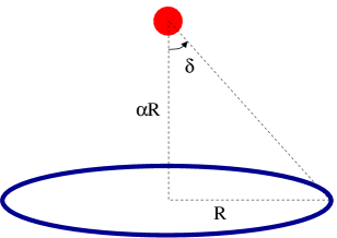
Figure 3: The configuration black ring with an off-set black hole on its axis. The parameter, $\alpha$, is related to the angle of approach, $\delta$, by $\alpha\equiv\cot{\rm\delta}$.

The total charge of the combined system is independent of $\alpha$ and is given by (54). Similarly, the entropy of the black ring is still given by (58) and (59), but now with $J_{T}$ defined by:

$$J_{T}~{}=~{}J_{\Delta}~{}+~{}{n^{I}N^{\rm BH}_{I}\over{1+\alpha^{2}}}~{}\equiv~{}{R^{2}L^{4}\over l_{p}^{6}}\,\Big{(}\sum n^{I}\Big{)}~{}+~{}{n^{I}N^{\rm BH}_{I}\over{1+\alpha^{2}}}\,.$$ (63)

The horizon area of the black hole is unmodified by the presence of the black ring and, in particular, its dependence on $\alpha$ only comes via $J_{T}$. Thus, for an adiabatic process, the quantity, ${\cal M}$, in (59) must remain fixed, and therefore $J_{T}$ must remain fixed. This is consistent with identifying $J_{T}$ as the intrinsic angular momentum of the ring.

The two angular momenta of the system are:

$$J_{1} ~{}=~{} J_{T}~{}+~{}\Big{(}{\textstyle{1\over 6}}\displaystyle\,C_{IJK}n^{I}n^{J}n^{K}~{}+~{}{\textstyle{1\over 2}}\displaystyle\,\overline{N}_{I}n^{I}~{}+~{}J^{\rm BMPV}\Big{)}\,\,,$$ (64)

$$J_{2} ~{}=~{} -\Big{(}{\textstyle{1\over 6}}\displaystyle\,C_{IJK}n^{I}n^{J}n^{K}~{}+~{}{\textstyle{1\over 2}}\displaystyle\,\overline{N}_{I}n^{I}~{}+~{}{N^{\rm BH}_{I}n^{I}\over{1+\alpha^{2}}}~{}+~{}J^{\rm BMPV}\Big{)}\,.$$ (65)

If we change the separation of the black hole and black ring while preserving the axial symmetry, that is, if we vary $\alpha$, then the symmetry requires $J_{1}$ to be conserved. Once again we see that this means that $J_{T}$ must remain fixed.

The constancy of $J_{T}$ along with (63) imply that as the black hole is brought near the black ring, the embedding radius of the latter, $R$, must change according to:

$$R^{2}~{}=~{}{l_{p}^{6}\over L^{4}}\,\,\big{(}\sum n^{I}\big{)}^{-1}\,\Big{(}J_{T}-{n^{I}N^{\rm BH}_{I}\over{1+\alpha^{2}}}\Big{)}\,.$$ (66)

For fixed microscopic charges this formula gives the radius of the ring as a function of the parameter $\alpha$. The black hole will merge with the black ring if and only if $R$ vanishes for some value of $\alpha$. That is, if and only if

$$J_{T}~{}\leq~{}n^{I}N^{\rm BH}_{I}\,.$$ (67)

The vanishing of $R$ suggests that the ring is pinching off, however, in the physical metric, (29), the ring generically has finite size as it settles onto the horizon of the black hole. Indeed, the value of $\alpha=\tan\zeta$ at the merger determines the latitude, $\zeta$, at which the ring settles on the black hole. If it occurs at $\alpha=0$ then the ring merges by grazing the black hole at the equator.

At merger ($R=0$) one can see that $J_{1}=J_{2}$ and so the resulting object will have $J_{1}=J_{2}$ given by (64). This will be a BMPV black hole and its electric charges are simply given by (54). We can therefore use (1) to determine the final entropy after the merger. Note that the process we are considering is adiabatic up to the point where the ring touches the horizon of the black hole. The process of swallowing the ring is not necessarily adiabatic, but we assume that the black hole does indeed swallow the black ring and we can then compute the entropy from the charges and angular momentum of the resulting BMPV black hole.

In general, the merger of a black hole and a black ring is irreversible, that is, the total horizon area increases in the process. However, there is precisely one situation in which the merger is reversible, and that requires all of the following to be true:

1. The ring must have zero horizon area (with a slight abuse of terminology we will also refer to such rings as supertubes).

2. The black hole that one begins with must have zero horizon area, i.e. it must be maximally spinning.

3. The ring must meet the black hole by grazing it at the equator.

4. There are two integers, $\bar{P}$ and $P^{BH}$ such that

   $$\overline{N}_{I}~{}=~{}{\overline{P}\over n^{I}}\qquad{\rm and}\qquad N^{BH}_{I}~{}=~{}{P^{BH}\over n^{I}}\,,\qquad I=1,2,3\,.$$ (68)

If all of these conditions are met then the end result is also a maximally spinning BMPV black hole and hence also has zero horizon area.

Note that the last condition implies that

$$N_{I}~{}\equiv~{}\overline{N}_{I}+{\textstyle{1\over 2}}\displaystyle\,C_{IJK}\,n^{J}\,n^{K}~{}=~{}{(\overline{P}+n^{1}\,n^{2}\,n^{3})\over n^{I}}\,,$$ (69)

and therefore the electric charges of black ring and its charges dissolved in fluxes (${1\over 2}\,C_{IJK}\,n^{J}\,n^{K}$) must both be aligned exactly parallel to the electric charges of the black hole. Conversely, if conditions 1–3 are satisfied, but the charge vectors of the black hole and black ring are not parallel then the merger will be irreversible. This observation will be important in Section 8.

4 Geometric interlude: Four-dimensional black holes and five-dimensional foam

In Section 3.1 we observed that supersymmetry allows us to take the base-space metric to be any hyper-Kähler metric. There are certainly quite a number of interesting four-dimensional hyper-Kähler metrics and in particular, there are the multi-centered Gibbons-Hawking metrics. These provide examples of asymptotically locally Euclidean (ALE) and asymptotically locally flat (ALF) spaces, which are asymptotic to ${R}^{4}/{Z}_{n}$ and ${R}^{3}\times S^{1}$ respectively. Using ALF metrics provides a smooth way to transition between a five-dimensional and a four-dimensional interpretation of a certain configurations. Indeed, the size of the $S^{1}$ is usually a modulus of a solution, and thus is freely adjustable. When this size is large compared to the size of the source configuration, this configuration is essentially five-dimensional; if the $S^{1}$ is small, then the configuration has a four-dimensional description.

We noted earlier that a regular, Riemannian, hyper-Kähler metric that is asymptotic to flat ${R}^{4}$ is necessarily flat ${R}^{4}$ globally. The non-trivial ALE metrics get around this by having a discrete identification at infinity but, as a result, do not have an asymptotic structure that lends itself to a space-time interpretation. However, there is an unwarranted assumption here: One should remember that the goal is for the five-metric (29) to be regular and Lorentzian and this might be achievable if singularities of the four-dimensional base space were canceled by the warp factors. More specifically, we are going to consider base-space metrics (30) whose overall sign is allowed to change in interior regions. That is, we are going to allow the signature to flip from $+4$ to $-4$. We will call such metrics ambipolar.

The potentially singular regions could actually be regular if the warp factors, $Z_{I}$, all flip sign whenever the four-metric signature flips. Indeed, we suspect that the desired property may follow quite generally from the BPS equations through the four-dimensional dualization on the right-hand side of (38). Obviously, there are quite a number of details to be checked before complete regularity is proven, but we will see below that this can be done for ambipolar Gibbons-Hawking metrics.

Because of these two important applications, we now give a review of Gibbons-Hawking geometries [56, 67] and their elementary ambipolar generalization. These metrics have the virtue of being simple enough for very explicit computation and yet capture some extremely interesting physics.

4.1 Gibbons-Hawking metrics

Gibbons-Hawking metrics have the form of a $U(1)$ fibration over a flat ${R}^{3}$ base:

$$h_{\mu\nu}dx^{\mu}dx^{\nu}~{}=~{}V^{-1}\,\big{(}d\psi+\vec{A}\cdot d\vec{y}\big{)}^{2}~{}+~{}V\,(dx^{2}+dy^{2}+dz^{2})\,,$$ (70)

where we write $\vec{y}=(x,y,z)$. The function, $V$, is harmonic on the flat ${R}^{3}$ while the connection, $A=\vec{A}\cdot d\vec{y}$, is related to $V$ via

$$\vec{\nabla}\times\vec{A}~{}=~{}\vec{\nabla}V\,.$$ (71)

This family of metrics is the unique set of hyper-Kähler metrics with a tri-holomorphic $U(1)$ isometry. Moreover, four-dimensional hyper-Kähler manifolds with $U(1)\times U(1)$ symmetry must, at least locally, be Gibbons-Hawking metrics with an extra $U(1)$ symmetry around an axis in the ${R}^{3}$ [68].

In the standard form of the Gibbons-Hawking metrics one takes $V$ to have a finite set of isolated sources. That is, let $\vec{y}^{(j)}$ be the positions of the source points in the ${R}^{3}$ and let $r_{j}\equiv|\vec{y}-\vec{y}^{(j)}|$. Then one takes:

$$V=\varepsilon_{0}~{}+~{}\sum_{j=1}^{N}\,{q_{j}\over r_{j}}\,,$$ (72)

where one usually takes $q_{j}\geq 0$ to ensure that the metric is Riemannian (positive definite). We will later relax this restriction. There appear to be singularities in the metric at $r_{j}=0$, however, if one changes to polar coordinates centered at $r_{j}=0$ with radial coordinate to $\rho=2\sqrt{|\vec{y}-\vec{y}^{(j)}|}$, then the metric is locally of the form:

$$ds_{4}^{2}~{}\sim~{}d\rho^{2}~{}+~{}\rho^{2}\,d\Omega_{3}^{2}\,,$$ (73)

where $d\Omega_{3}^{2}$ is the standard metric on $S^{3}/{Z}_{|q_{j}|}$. In particular, this means that one must have $q_{j}\in{Z}$ and if $|q_{j}|=1$ then the space looks locally like ${R}^{4}$. If $|q_{j}|\neq 1$ then there is an orbifold singularity, but since this is benign in string theory, we will view such backgrounds as regular.

If $\varepsilon_{0}\neq 0$, then $V\to\varepsilon_{0}$ at infinity and so the metric (70) is asymptotic to flat ${R}^{3}\times S^{1}$, that is, the base is asymptotically locally flat (ALF). The five-dimensional space-time is thus asymptotically compactified to a four-dimensional space-time. This a standard Kaluza-Klein reduction and the gauge field, $\vec{A}$, yields a non-trivial, four-dimensional Maxwell field whose sources, from the ten-dimensional perspective, are simply D6 branes. In Section 5.6 we will make extensive use of of the fact that introducing a constant term into $V$ yields a further compactification and through this we can relate five-dimensional physics to four-dimensional physics.

Now suppose that one has $\varepsilon_{0}=0$. At infinity in ${R}^{3}$ one has $V\sim q_{0}/r$, where $r\equiv|\vec{y}|$ and

$$q_{0}~{}\equiv~{}\sum_{j=1}^{N}\,q_{j}\,.$$ (74)

Hence spatial infinity in the Gibbons-Hawking metric also has the form (73), where

$$r~{}=~{}{\textstyle{1\over 4}}\displaystyle\,\rho^{2}\,,$$ (75)

and $d\Omega_{3}^{2}$ is the standard metric on $S^{3}/{Z}_{|q_{0}|}$. For the Gibbons-Hawking metric to be asymptotic to the positive definite, flat metric on ${R}^{4}$ one must have $q_{0}=1$. Note that for the Gibbons-Hawking metrics to be globally positive definite one would also have to take $q_{j}\geq 0$ and thus the only such metric would have to have $V\equiv{1\over r}$. The metric (70) is then the flat metric on ${R}^{4}$ globally, as can be seen by using the change of variables (75). The only way to get non-trivial metrics that are asymptotic to flat ${R}^{4}$ is by taking some of the $q_{j}\in{Z}$ to be negative.

4.2 Homology and cohomology

The multi-center Gibbons-Hawking (GH) metrics also contain ${1\over 2}N(N-1)$ topologically non-trivial two-cycles, $\Delta_{ij}$, that run between the GH centers. These two-cycles can be defined by taking any curve, $\gamma_{ij}$, between $\vec{y}^{(i)}$ and $\vec{y}^{(j)}$ and considering the $U(1)$ fiber of (70) along the curve. This fiber collapses to zero at the GH centers, and so the curve and the fiber sweep out a $2$-sphere (up to ${Z}_{|q_{j}|}$ orbifolds). See Fig. 4. These spheres intersect one another at the common points $\vec{y}^{(j)}$. There are $(N-1)$ linearly independent homology two-spheres, and the set $\Delta_{i\,(i+1)}$ represents a basis.

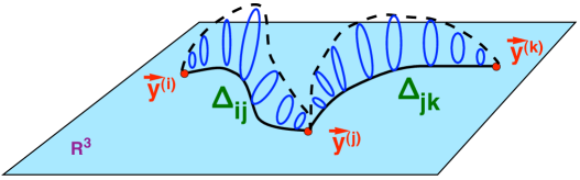
Figure 4: This figure depicts some non-trivial cycles of the Gibbons-Hawking geometry. The behaviour of the $U(1)$ fiber is shown along curves between the sources of the potential, $V$. Here the fibers sweep out a pair of intersecting homology spheres.

It is also convenient to introduce a set of frames

$$\hat{e}^{1}~{}=~{}V^{-{1\over 2}}\,(d\psi~{}+~{}A)\,,\qquad\hat{e}^{a+1}~{}=~{}V^{1\over 2}\,dy^{a}\,,\quad a=1,2,3\,.$$ (76)

and two associated sets of two-forms:

$$\Omega_{\pm}^{(a)}~{}\equiv~{}\hat{e}^{1}\wedge\hat{e}^{a+1}~{}\pm~{}{\textstyle{1\over 2}}\displaystyle\,\epsilon_{abc}\,\hat{e}^{b+1}\wedge\hat{e}^{c+1}\,,\qquad a=1,2,3\,.\$$ (77)

The two-forms, $\Omega_{-}^{(a)}$, are anti-self-dual, harmonic and non-normalizable and they define the hyper-Kähler structure on the base. The forms, $\Omega_{+}^{(a)}$, are self-dual and can be used to construct harmonic fluxes that are dual to the two-cycles. Consider the self-dual two-form:

$$\Theta~{}\equiv~{}\sum_{a=1}^{3}\,\big{(}\partial_{a}\big{(}V^{-1}\,H\big{)}\big{)}\,\Omega_{+}^{(a)}\,.$$ (78)

Then $\Theta$ is closed (and hence co-closed and harmonic) if and only if $H$ is harmonic in ${R}^{3}$, i.e. $\nabla^{2}H=0$. We now have the choice of how to distribute sources of $H$ throughout the ${R}^{3}$ base of the GH space; such a distribution may correspond to having multiple black rings and black holes in this space. Nevertheless, if we want to obtain a geometry that has no singularities and no horizons, $\Theta$ has to be regular, and this happens if and only if $H/V$ is regular; this occurs if and only if $H$ has the form:

$$H~{}=~{}h_{0}~{}+~{}\sum_{j=1}^{N}\,{h_{j}\over r_{j}}\,.$$ (79)

Also note that the “gauge transformation:”

$$H~{}\to~{}H~{}+~{}c\,V\,,$$ (80)

for some constant, $c$, leaves $\Theta$ unchanged, and so there are only $N$ independent parameters in $H$. In addition, if $\varepsilon=0$ then one must take $h_{0}=0$ for $\Theta$ to remain finite at infinity. The remaining $(N-1)$ parameters then describe harmonic forms that are dual to the non-trivial two-cycles. If $\varepsilon\neq 0$ then the extra parameter is that of a Maxwell field whose gauge potential gives the Wilson line around the $S^{1}$ at infinity.

Exercise:   Show that the two-form, $\Theta$, defined by (78) and (79) is normalizable on standard GH spaces (with $V>0$ everywhere). That is, show that $\Theta$ square integrable: $$\int\Theta\wedge\Theta~{}<~{}\infty\,,$$ (81) where the integral is taken of the whole GH base space.

It is straightforward to find a local potential such that $\Theta=dB$:

$$B~{}\equiv~{}V^{-1}\,H\,(d\psi~{}+~{}A)~{}+~{}\vec{\xi}\cdot d\vec{y}\,,$$ (82)

where

$$\vec{\nabla}\times\vec{\xi}~{}=~{}-\vec{\nabla}H\,.$$ (83)

Hence, $\vec{\xi}$ is a vector potential for magnetic monopoles located at the singular points of $H$.

To determine how these fluxes thread the two-cycles we need the explicit forms for the vector potential, $B$, and to find these we first need the vector fields, $\vec{v}_{i}$, that satisfy:

$$\vec{\nabla}\times\vec{v}_{i}~{}=~{}\vec{\nabla}\,\bigg{(}{1\over r_{i}}\bigg{)}\,.$$ (84)

One then has:

$$\vec{A}~{}=~{}\sum_{j=1}^{N}\,q_{j}\,\vec{v}_{j}\,,\qquad\vec{\xi}~{}=~{}\sum_{j=1}^{N}\,h_{j}\,\vec{v}_{j}\,.$$ (85)

If we choose coordinates so that $\vec{y}^{(i)}~{}=~{}(0,0,a)$ and let $\phi$ denote the polar angle in the $(x,y)$-plane, then:

$$\vec{v}_{i}\cdot d\vec{y}~{}=~{}\Big{(}{(z-a)\over r_{i}}~{}+~{}c_{i}\Big{)}\,d\phi\,,$$ (86)

where $c_{i}$ is a constant. The vector field, $\vec{v}_{i}$, is regular away from the $z$-axis, but has a Dirac string along the $z$-axis. By choosing $c_{i}$ we can cancel the string along the positive or negative $z$-axis, and by moving the axis we can arrange these strings to run in any direction we choose, but they must start or finish at some $\vec{y}^{(i)}$, or run out to infinity.

Now consider what happens to $B$ in the neighborhood of $\vec{y}^{(i)}$. Since the circles swept out by $\psi$ and $\phi$ are shrinking to zero size, the string singularities near $\vec{y}^{(i)}$ are of the form:

$$B~{}\sim~{}{h_{i}\over q_{i}}\,\Big{(}d\psi+q_{i}\,\Big{(}{(z-a)\over r_{i}}+c_{i}\Big{)}\,d\phi\Big{)}~{}-~{}h_{i}\,\Big{(}{(z-a)\over r_{i}}+c_{i}\Big{)}\,d\phi~{}\sim~{}{h_{i}\over q_{i}}\,d\psi\,.$$ (87)

This shows that the vector, $\vec{\xi}$, in (82) cancels the string singularities in the ${R}^{3}$. The singular components of $B$ thus point along the $U(1)$ fiber of the GH metric.

Choose any curve, $\gamma_{ij}$, between $\vec{y}^{(i)}$ and $\vec{y}^{(j)}$ and define the two-cycle, $\Delta_{ij}$, as in Fig. 4. If one has $V>0$ then the vector field, $B$, is regular over the whole of $\Delta_{ij}$ except at the end-points, $\vec{y}^{(i)}$ and $\vec{y}^{(j)}$. Let $\mathaccent 866{\Delta}_{ij}$ be the cycle $\Delta_{ij}$ with the poles excised. Since $\Theta$ is regular at the poles, then the expression for the flux, $\Pi_{ij}$, through $\Delta_{ij}$ can be obtained as follows:

$$\Pi_{ij} ~{}\equiv~{} {1\over 4\,\pi}\,\int_{\Delta_{ij}}\,\Theta~{}=~{}{1\over 4\,\pi}\,\int_{\mathaccent 866{\Delta}_{ij}}\,\Theta~{}=~{}{1\over 4\,\pi}\,\int_{\partial\mathaccent 866{\Delta}_{ij}}\,B$$ (88)

$$~{}=~{} {1\over 4\,\pi}\,\int_{0}^{4\pi}\,d\psi\,\big{(}B|_{y^{(j)}}~{}-~{}B|_{y^{(i)}}\big{)}~{}=~{}\bigg{(}{h_{j}\over q_{j}}~{}-~{}{h_{i}\over q_{i}}\bigg{)}\,.$$

We have normalized these periods for later convenience.

On an ambipolar GH space where the cycle runs between positive and negative GH points, the flux, $\Theta$, and the potential $B$ are both singular when $V=0$ and so this integral is a rather formal object. However, we will see in Section 6.3 that when we extend to the five-dimensional metric, the physical flux of the complete Maxwell field combines $\Theta$ with another term so that the result is completely regular. Moreover, the physical flux through the cycle is still given by (88). We will therefore refer to (88) as the magnetic flux even in ambipolar metrics and we will see that such fluxes are directly responsible for holding up the cycles

5 Solutions on a Gibbons-Hawking base

5.1 Solving the BPS equations

Our task now is to solve the BPS equations (37)–(39) but now with a Gibbons-Hawking base metric. Such solutions have been derived before for positive-definite Gibbons-Hawking metrics [69, 55], and it is trivial to generalize to the ambipolar form. For the present we will not impose any conditions on the sources of the BPS equations.

In Section 4.2 we saw that there was a simple way to obtain self-dual two-forms, $\Theta^{(I)}$, that satisfy (37). That is, we introduce three harmonic functions, $K^{I}$, on ${R}^{3}$ that satisfy ${\bf\nabla}^{2}K^{I}=0$, and define $\Theta^{(I)}$ as in (78) by replacing $H$ with $K^{I}$. We will not, as yet, assume any specific form for $K^{I}$.

Exercise:  Substitute these two-forms into (38) and show that the resulting equation has the solution: $$Z_{I}~{}=~{}{\textstyle{1\over 2}}\displaystyle\,C_{IJK}\,V^{-1}\,K^{J}K^{K}~{}+~{}L_{I}\,,$$ (89) where the $L_{I}$ are three more independent harmonic functions.

We now write the one-form, $k$, as:

$$k~{}=~{}\mu\,(d\psi+A)~{}+~{}\omega$$ (90)

and then (39) becomes:

$$\vec{\nabla}\times\vec{\omega}~{}=~{}(V\vec{\nabla}\mu~{}-~{}\mu\vec{\nabla}V)~{}-~{}\,V\,\sum_{I=1}^{3}\,Z_{I}\,\vec{\nabla}\bigg{(}{K^{I}\over V}\bigg{)}\,.$$ (91)

Taking the divergence yields the following equation for $\mu$:

$$\nabla^{2}\mu~{}=~{}\,V^{-1}\,\vec{\nabla}\cdot\bigg{(}V\sum_{I=1}^{3}\,Z_{I}~{}\vec{\nabla}{K^{I}\over V}\bigg{)}\,,$$ (92)

which is solved by:

$$\mu~{}=~{}{\textstyle{1\over 6}}\displaystyle\,C_{IJK}\,{K^{I}K^{J}K^{K}\over V^{2}}~{}+~{}{1\over 2\,V}\,K^{I}L_{I}~{}+~{}M\,,$$ (93)

where $M$ is yet another harmonic function on ${R}^{3}$. Indeed, $M$ determines the anti-self-dual part of $dk$ that cancels out of (39). Substituting this result for $\mu$ into (91) we find that $\omega$ satisfies:

$$\vec{\nabla}\times\vec{\omega}~{}=~{}V\vec{\nabla}M~{}-~{}M\vec{\nabla}V~{}+~{}{\textstyle{1\over 2}}\displaystyle\,(K^{I}\vec{\nabla}L_{I}-L_{I}\vec{\nabla}K^{I})\,.$$ (94)

The integrability condition for this equation is simply the fact that the divergence of both sides vanish, which is true because $K^{I},L_{I},M$ and $V$ are harmonic.

5.2 Some properties of the solution

The solution is thus characterized by the harmonic functions $K^{I},L_{I}$, $V$ and $M$. The gauge invariance, (80), extends in a straightforward manner to the complete solution:

$$K^{I} ~{}\rightarrow~{} K^{I}~{}+~{}c^{I}\,V\,,$$

$$L_{I} ~{}\rightarrow~{} L_{I}~{}-~{}C_{IJK}\,c^{J}\,K^{K}~{}-~{}{\textstyle{1\over 2}}\displaystyle\,C_{IJK}\,c^{J}\,c^{K}\,V\,,$$

$$M ~{}\rightarrow~{} M-{\textstyle{1\over 2}}\displaystyle\,c^{I}\,L_{I}+{1\over 12}\,C_{IJK}\left(V\,c^{I}\,c^{J}\,c^{K}+3\,c^{I}\,c^{J}\,K^{K}\right)\,,$$ (95)

where the $c^{I}$ are three arbitrary constants.

The eight functions that give the solution may also be identified with the eight independent parameters in the 56 of the $E_{7(7)}$ duality group in four dimensions:

$$x_{12} ~{}=~{} L_{1}\,,\qquad x_{34}~{}=~{}L_{2}\,,\qquad x_{56}~{}=~{}L_{3}\,,\qquad x_{78}~{}=~{}-V\,,$$

$$y_{12} ~{}=~{} K^{1}\,,\qquad y_{34}~{}=~{}K^{2}\,,\qquad y_{56}~{}=~{}K^{3}\,,\qquad y_{78}~{}=~{}2\,M\,.$$ (96)

With these identifications, the right-hand side of (94) is the symplectic invariant of the 56 of $E_{7(7)}$:

$$\vec{\nabla}\times\vec{\omega}~{}=~{}{\textstyle{1\over 4}}\displaystyle\,\sum_{A,B=1}^{8}\,(y_{AB}\vec{\nabla}x_{AB}~{}-~{}x_{AB}\vec{\nabla}y_{AB})\,.$$ (97)

We also note that the quartic invariant of the 56 of $E_{7(7)}$ is determined by:

$$J_{4} ~{}=~{} -{1\over 4}(x_{12}y^{12}+x_{34}y^{34}+x_{56}y^{56}+x_{78}y^{78})^{2}-x_{12}x_{34}x_{56}x_{78}$$ (98)

$$-y^{12}y^{34}y^{56}y^{78}+x_{12}x_{34}y^{12}y^{34}+x_{12}x_{56}y^{12}y^{56}+x_{34}x_{56}y^{34}y^{56}$$

$$+x_{12}x_{78}y^{12}y^{78}+x_{34}x_{78}y^{34}y^{78}+x_{56}x_{78}y^{56}y^{78}\,,$$

and we will see that this plays a direct role in the expression for the scale of the $U(1)$ fibration. It also plays a central role in the expression for the horizon area of a four-dimensional black hole [70].

In principle we can choose the harmonic functions $K^{I},L_{I}$ and $M$ to have sources that are localized anywhere on the base. These solutions then have localized brane sources, and include, for example, supertubes and black rings in Taub-NUT [27, 58, 59, 60], which we will review in Section 5.5. Such solutions also include more general multi-center black hole configurations in four dimensions, of the type considered by Denef and collaborators [71].

Nevertheless, our focus for the moment is on obtaining smooth horizonless solutions, which correspond to microstates of black holes and black rings and we choose the harmonic functions so that there are no brane charges anywhere, and all the charges come from the smooth cohomological fluxes that thread the non-trivial cycles.

5.3 Closed time-like curves

To look for the presence of closed time-like curves in the metric one considers the space-space components of the metric given by (28), (29) and (70). That is, one goes to the space-like slices obtained by taking $t$ to be a constant. The $T^{6}$ directions immediately yield the requirement that $Z_{I}Z_{J}>0$ while the metric on the four-dimensional base reduces to:

$$ds^{2}_{4} = -W^{-4}\,\big{(}\mu(d\psi+A)+\omega\big{)}^{2}$$ (99)

$$~{}+~{}{W^{2}V^{-1}}\big{(}d\psi+A\big{)}^{2}+W^{2}V\big{(}dr^{2}+r^{2}d\theta^{2}+r^{2}\sin^{2}\theta\,d\phi^{2}\big{)}\,,$$

where we have chosen to write the metric on ${R}^{3}$ in terms of a generic set of spherical polar coordinates, $(r,\theta,\phi)$ and where we have defined the warp-factor, $W$, by:

$$W~{}\equiv~{}(Z_{1}\,Z_{2}\,Z_{3})^{1/6}\,.$$ (100)

There is some potentially singular behavior arising from the fact that the $Z_{I}$, and hence $W$, diverge on the locus, $V=0$ (see (89)). However, one can show that if one expands the metric (99) and uses the expression, (93), then all the dangerous divergent terms cancel and the metric is regular. We will discuss this further below and in Section 5.4.

Expanding (99) leads to:

$$ds^{2}_{4} = W^{-4}\,(W^{6}V^{-1}-\mu^{2})\Big{(}d\psi+A-{\mu\,\omega\over W^{6}V^{-1}-\mu^{2}}\Big{)}^{2}-{W^{2}\,V^{-1}\over W^{6}V^{-1}-\mu^{2}}\,\omega^{2}$$ (101)

$$~{}+~{}W^{2}V\big{(}dr^{2}+r^{2}d\theta^{2}+r^{2}\sin^{2}\theta\,d\phi^{2}\big{)}$$

$$= {{\cal Q}\over W^{4}V^{2}}\Big{(}d\psi+A-{\mu\,V^{2}\over{\cal Q}}\,\omega\Big{)}^{2}~{}+~{}W^{2}V\Big{(}r^{2}\sin^{2}\theta\,d\phi^{2}-{\omega^{2}\over{\cal Q}}\Big{)}$$

$$~{}+~{}W^{2}V(dr^{2}+r^{2}d\theta^{2})\,,$$

where we have introduced the quantity:

$${\cal Q}~{}\equiv~{}W^{6}\,V~{}-~{}\mu^{2}\,V^{2}~{}=~{}Z_{1}Z_{2}Z_{3}V~{}-~{}\mu^{2}\,V^{2}\,.$$ (102)

Upon evaluating ${\cal Q}$ as a function of the harmonic functions that determine the solution one obtains a beautiful result:

$${\cal Q} ~{}=~{} -M^{2}\,V^{2}-{\textstyle{1\over 3}}\displaystyle\,M\,C_{IJK}{K^{I}}\,{K^{J}}\,{K^{k}}-M\,V\,{K^{I}}\,{L_{I}}-{\textstyle{1\over 4}}\displaystyle\,(K^{I}L_{I})^{2}$$ (103)

$$\quad+{\textstyle{1\over 6}}\displaystyle\,VC^{IJK}L_{I}L_{J}L_{K}+{\textstyle{1\over 4}}\displaystyle\,C^{IJK}C_{IMN}L_{J}L_{K}K^{M}K^{N}$$

with $C^{IJK}\equiv C_{IJK}$. We can straightforwardly see that when we consider M-theory compactified on $T^{6}$, then $C^{IJK}=|\epsilon^{IJK}|$, and ${\cal Q}$ is nothing other than the $E_{7(7)}$ quartic invariant (98) where the $x$’s and $y$’s are identified as in (96). This is expected from the fact that the solutions on a GH base have an extra $U(1)$ invariance, and hence can be thought of as four-dimensional. The four-dimensional supergravity obtained by compactifying M-theory on $T^{7}$ is $N=8$ supergravity, which has an $E_{7(7)}$ symmetry group. Of course, the analysis above and in particular equation (103) are valid for solutions of arbitrary five-dimensional $U(1)^{N}$ ungauged supergravities on a GH base. More details on the explicit relation for general theories can be found in [72].

Exercise:  Check that ${\cal Q}$ is invariant under the gauge transformation (95)

Observe that (101) only involves $V$ in the combinations $W^{2}V$ and ${\cal Q}$ and both of these are regular as $V\to 0$. Thus, at least the spatial metric is regular at $V=0$. In Section 5.4 we will show that the complete solution is regular as one passes across the surface $V=0$.

From (101) and (28) we see that to avoid CTC’s, the following inequalities must be true everywhere:

$${\cal Q}~{}\geq~{}0\,,\quad W^{2}\,V~{}\geq~{}0\,,\quad\big{(}Z_{J}\,Z_{K}\,Z_{I}^{-2}\big{)}^{1\over 3}~{}=~{}W^{2}Z_{I}^{-1}~{}\geq~{}0\,,\ \ I=1,2,3\,.$$ (104)

The last two conditions can be subsumed into:

$$V\,Z_{I}~{}=~{}{\textstyle{1\over 2}}\displaystyle\,C_{IJK}\,K^{J}\,K^{K}~{}+~{}L_{I}\,V~{}\geq~{}0\,,\qquad I=1,2,3\,.$$ (105)

The obvious danger arises when $V$ is negative. We will show in the next sub-section that all these quantities remain finite and positive in a neighborhood of $V=0$, despite the fact that $W$ blows up. Nevertheless, these quantities could possibly be negative away from the $V=0$ surface. While we will, by no means, make a complete analysis of the positivity of these quantities, we will discuss it further in Section 6.5, and show that (105) does not present a significant problem in a simple example. One should also note that ${\cal Q}\geq 0$ requires $\prod_{I}(VZ_{I})\geq\mu^{2}V^{4}$, and so, given (105), the constraint ${\cal Q}\geq 0$ is still somewhat stronger.

Also note that there is a danger of CTC’s arising from Dirac-Misner strings in $\omega$. That is, near $\theta=0,\pi$ the $-\omega^{2}$ term could be dominant unless $\omega$ vanishes on the polar axis. We will analyze this issue completely when we consider bubbled geometries in Section 6.

Finally, one can also try to argue [29] that the complete metric is stably causal and that the $t$ coordinate provides a global time function [73]. In particular, $t$ will then be monotonic increasing on future-directed non-space-like curves and hence there can be no CTC’s. The coordinate $t$ is a time function if and only if

$$-g^{\mu\nu}\partial_{\mu}t\,\partial_{\nu}t=-g^{tt}=(W^{2}V)^{-1}({\cal Q}-\omega^{2})>0\,,$$ (106)

where $\omega$ is squared using the ${R}^{3}$ metric. This is obviously a slightly stronger condition than ${\cal Q}\geq 0$ in (104).

5.4 Regularity of the solution and critical surfaces

As we have seen, the general solutions we will consider have functions, $V$, that change sign on the ${R}^{3}$ base of the GH metric. Our purpose here is to show that such solutions are completely regular, with positive definite metrics, in the regions where $V$ changes sign. As we will see the “critical surfaces,” where $V$ vanishes are simply a set of completely harmless, regular hypersurfaces in the full five-dimensional geometry.

The most obvious issue is that if $V$ changes sign, then the overall sign of the metric (70) changes and there might be whole regions of closed time-like curves when $V<0$. However, we remarked above that the warp factors, in the form of $W$, prevent this from happening. Specifically, the expanded form of the complete, eleven-dimensional metric when projected onto the GH base yields (101). Moreover

$$W^{2}\,V~{}=~{}(Z_{1}\,Z_{2}\,Z_{3}\,V^{3})^{1\over 3}~{}\sim~{}((K_{1}\,K_{2}\,K_{3})^{2})^{1\over 3}$$ (107)

on the surface $V=0$. Hence $W^{2}V$ is regular and positive on this surface, and therefore the space-space part (101) of the full eleven-dimensional metric is regular.

There is still the danger of singularities at $V=0$ for the other background fields. We first note that there is no danger of such singularities being hidden implicitly in the $\vec{\omega}$ terms. Even though (91) suggests that the source of $\vec{\omega}$ is singular at $V=0$, we see from (94) that the source is regular at $V=0$ and thus there is nothing hidden in $\vec{\omega}$. We therefore need to focus on the explicit inverse powers of $V$ in the solution.

The factors of $V$ cancel in the torus warp factors, which are of the form $(Z_{I}Z_{J}Z_{K}^{-2})^{1\over 3}$. The coefficient of $(dt+k)^{2}$ is $W^{-4}$, which vanishes as $V^{2}$. The singular part of the cross term, $dt\,k$, is $\mu\,dt\,(d\psi+A)$, which, from (93), diverges as $V^{-2}$, and so the overall cross term, $W^{-4}dt\,k$, remains finite at $V=0$.

So the metric is regular at critical surfaces. The inverse metric is also regular at $V=0$ because the $dt\,d\psi$ part of the metric remains finite and so the determinant is non-vanishing.

This surface is therefore not an event horizon even though the time-like Killing vector defined by translations in $t$ becomes null when $V=0$. Indeed, when a metric is stationary but not static, the fact that $g_{tt}$ vanishes on a surface does not make it an event horizon (the best known example of this is the boundary of the ergosphere of the Kerr metric). The necessary condition for a surface to be a horizon is rather to have $g^{rr}=0$, where $r$ is the coordinate transverse to this surface. This is clearly not the case here.

Hence, the surface given by $V=0$ is like a boundary of an ergosphere, except that the solution has no ergosphere because this Killing vector is time-like on both sides and does not change character across the critical surface. In the Kerr metric the time-like Killing vector becomes space-like and this enables energy extraction by the Penrose process. Here there is no ergosphere and so energy extraction is not possible, as is to be expected from a BPS geometry.

At first sight, it does appear that the Maxwell fields are singular on the surface $V=0$. Certainly the “magnetic components,” $\Theta^{(I)}$, (see (78)) are singular when $V=0$. However, one knows that the metric is non-singular and so one should expect that the singularity in the $\Theta^{(I)}$ to be unphysical. This intuition is correct: One must remember that the complete Maxwell fields are the $A^{(I)}$, and these are indeed non-singular at $V=0$. One finds that the singularities in the “magnetic terms” of $A^{(I)}$ are canceled by singularities in the “electric terms” of $A^{(I)}$, and this is possible at $V=0$ precisely because $g_{tt}$ goes to zero, and so the magnetic and electric terms can communicate. Specifically, one has, from (36) and (82):

$$dA^{(I)}~{}=~{}d\,\bigg{(}B^{(I)}~{}-~{}{(dt+k)\over Z_{I}}\bigg{)}\,.$$ (108)

Near $V=0$ the singular parts of this behave as:

$$dA^{(I)} ~{}\sim~{} d\,\bigg{(}{K^{I}\over V}~{}-~{}{\mu\over Z_{I}}\bigg{)}\,(d\psi+A)$$ (109)

$$~{}\sim~{} d\,\bigg{(}{K^{I}\over V}~{}-~{}{K^{1}\,K^{2}\,K^{3}\over{\textstyle{1\over 2}}\displaystyle\,V\,C_{IJK}\,K^{J}\,K^{K}}\bigg{)}\,(d\psi+A)~{}\sim~{}0\,.$$

The cancellations of the $V^{-1}$ terms here occur for much the same reason that they do in the metric (101).

Therefore, even if $V$ vanishes and changes sign and the base metric becomes negative definite, the complete eleven-dimensional solution is regular and well-behaved around the $V=0$ surfaces. It is this fact that gets us around the uniqueness theorems for asymptotically Euclidean self-dual (hyper-Kähler) metrics in four dimensions, and as we will see, there are now a vast number of candidates for the base metric.

5.5 Black rings in Taub-NUT

Having analyzed the general form of solutions with a GH base, it is interesting to re-examine the black ring solution of Section 3.4 and rewrite it in the form discussed in Section 5.1 with a trivial GH base (with $V={1\over r}$). We do this because it is then elementary to generalize the solution to more complicated base spaces and most particularly to a Taub-NUT base. This will then illustrate a very important technique that makes it elementary to further compactify solutions to four-dimensional space-times and establish the relationship between four-dimensional and five-dimensional quantities. For pedagogical reasons, we will focus on the metric; details on the field strengths and the moduli can be found in [60].

Exercise:  Show that the black ring warp factors and rotation vector, when written in usual ${R}^{4}$ coordinates $$ds^{2}=d\tilde{r}^{2}+\tilde{r}^{2}(d\tilde{\theta}^{2}+\sin^{2}\tilde{\theta}d\tilde{\psi}^{2}+\cos^{2}\tilde{\theta}d\tilde{\phi}^{2})$$ (110) are given by: $\displaystyle Z_{I}$ $\displaystyle=$ $\displaystyle 1+{\overline{Q}_{I}\over\tilde{\Sigma}}+{1\over 2}C_{IJK}q^{J}q^{K}{\tilde{r}^{2}\over\tilde{\Sigma}^{2}}$ (111) $\displaystyle k$ $\displaystyle=$ $\displaystyle-{\tilde{r}^{2}\over 2\tilde{\Sigma}^{2}}\left(q^{I}\overline{Q}_{I}+{2q^{1}q^{2}q^{3}\tilde{r}^{2}\over\tilde{\Sigma}}\right)(\cos^{2}\tilde{\theta}\,d\tilde{\phi}+\sin^{2}\tilde{\theta}\,d\tilde{\psi})$ (112) $\displaystyle-$ $\displaystyle J_{T}\,{2\tilde{r}^{2}\sin^{2}\tilde{\theta}\over\tilde{\Sigma}(\tilde{r}^{2}+\mathaccent 869{R}^{2}+\tilde{\Sigma})}\,d\tilde{\psi}\,,$ (113) where $C_{IJK}=1$ for $(IJK)=(123)$ and permutations thereof, $${\tilde{\Sigma}\equiv\sqrt{(\tilde{r}^{2}-\mathaccent 869{R}^{2})^{2}+4\mathaccent 869{R}^{2}\tilde{r}^{2}\cos^{2}\tilde{\theta}}\,,}$$ (114) and $J_{T}\equiv J_{\tilde{\psi}}-J_{\tilde{\phi}}~{}$.

In the foregoing, we have written the solution in terms of the ring charges, $\overline{Q}_{I}$ and, as we have already noted, for the five-dimensional black ring these charges differ from the charges measured at infinity because of the charge “dissolved” in the M5-brane fluxes. The charges measured at infinity are $Q_{I}=\overline{Q}_{I}+{1\over 2}C_{IJK}q^{J}q^{K}$. We will also make a convenient choice of units in which $G_{5}={\pi\over 4}$, and choose the three $T^{2}$’s of the M-theory metric to have equal size.

Exercise:  Show that in these units the charges $Q_{I}$, $\overline{Q}_{I}$ and $q^{I}$ that appear in the supergravity warp factors are the same as the corresponding quantized brane charges.
Hint 1: Begin by relating $G_{11}$ and $G_{5}$ using the torus volumes.
Hint 2: You can cheat and use the relation between the charges in the supergravity formula and the integer quantized charges derived in [44] and summarized in (53). If you feel like doing honest character-building work, find the M2 charges by integrating $F_{7}$ over the corresponding $S^{3}\times T^{2}\times T^{2}$ at infinity; find the M5 charges by integrating $F_{4}$ over the corresponding $T^{2}\times S^{2}$, where the $S^{2}$ goes around the ring.
Hint 3: You can find the M5 dipole charges most easily if you use a coordinate system centered at $\Sigma=0$ described in equation (129) below.

From (66), the radius of the ring, $\mathaccent 869{R}$, and is related to $J_{T}$ by

$${J_{T}=(q^{1}+q^{2}+q^{3})\mathaccent 869{R}^{2}.}$$ (115)

We now perform a change of coordinates, to bring the black ring to a form that can easily be generalized to Taub-NUT. Define

$$\phi=\tilde{\phi}-\tilde{\psi},\quad\psi=2\tilde{\psi},\quad\theta=2\tilde{\theta},\quad\rho={\tilde{r}^{2}\over 4}\,,$$ (116)

where the ranges of these coordinates are given by

$$\theta\in(0,\pi),\quad(\psi,\phi)\cong(\psi+4\pi,\phi)\cong(\psi,\phi+2\pi)~{}.$$ (117)

Exercise:  Verify that when $V={1\over\rho}$, the coordinate change (116) transforms the metric in the first line of (123) to that of flat ${R}^{4}$.

In the new coordinates the black-ring metric is

$$ds^{2} = -(Z_{1}Z_{2}Z_{3})^{-2/3}(dt+k)^{2}+(Z_{1}Z_{2}Z_{3})^{1/3}h_{mn}dx^{m}dx^{n}\,,$$ (118)

$$Z_{I} = 1+{\overline{Q}_{I}\over 4\Sigma}+{1\over 2}C_{IJK}q^{J}q^{K}{\rho\over 4\Sigma^{2}}\,,$$ (119)

$$k = \mu\left(d\psi+(1+\cos\theta)d\phi\right)+\omega\,,$$ (120)

$$\mu = -{1\over 16}{\rho\over\Sigma^{2}}\left(q^{I}\overline{Q}_{I}+{2q^{1}q^{2}q^{3}\rho\over\Sigma}\right)+{J_{T}\over 16R}\left(1-{\rho\over\Sigma}-{R\over\Sigma}\right)\,,$$ (121)

$$\omega = -{J_{T}\rho\over 4\Sigma(\rho+R+\Sigma)}\sin^{2}\theta d\phi\,,$$ (122)

with

$$h_{mn}dx^{m}dx^{n} = V^{-1}\left(d\psi+(1+\cos\theta)d\phi\right)^{2}+V(d\rho^{2}+\rho^{2}(d\theta^{2}+\sin^{2}\theta d\phi^{2}))\,,$$ (123)

$$V = {1\over\rho}\,,\quad\Sigma=\sqrt{\rho^{2}+R^{2}+2R\rho\cos\theta}\,,\quad R={\mathaccent 869{R}^{2}\over 4}~{}.$$ (124)

Exercise:  Check that the solution (118) has the form described in Section 5.1 with the eight harmonic functions: $\displaystyle K^{I}$ $\displaystyle=$ $\displaystyle-{q^{I}\over 2\Sigma}\,,\qquad L_{I}=1+{\overline{Q}_{I}\over 4\Sigma}\,,$ (125) $\displaystyle M$ $\displaystyle=$ $\displaystyle{J_{T}\over 16}\left({1\over R}-{1\over\Sigma}\right)\,,\qquad V={1\over\rho}\,.$ (126)

We should also note for completeness that the conventions we use here for these harmonic functions are those of [60], and differ from those of [55] by various factors of two. When ${R}^{4}$ is written in Gibbons-Hawking form, the ring is sitting at a distance $R$ along the negative $z$-axis of the three-dimensional base. Adding more sources on the $z$ axis corresponds to making concentric black rings [76, 55].

Exercise:  Show that adding sources on the same side of the origin in the ${R}^{3}$ base of (123), correspond to rings that sit in the same ${R}^{2}$ inside ${R}^{4}$. Show that rings that sit in orthogonal ${R}^{2}$’s inside ${R}^{4}$ correspond to sources sitting on opposite sides of the origin of the ${R}^{3}$ base of (123).

To change the four-dimensional base metric into Taub-NUT one simply needs to add a constant, $h$, to the harmonic function $V$:

$$V~{}=~{}h+{1\over\rho}\,.$$ (127)

Since the functions in the metric are harmonic, equations (89), (90), (93), (94) and (126), still imply that we have a supersymmetric solution. Actually, in order to avoid both Dirac string singularities and closed time-like curves, the relation (115) between $J_{T}$ and the dipole charges must be modified to:

$${J_{T}\left(h+{1\over R}\right)=4(q^{1}+q^{2}+q^{3})\,.}$$ (128)

This is discussed in detail in [60, 59, 58] and in later sections here, but it follows because the absence of singularities in $\omega$ puts constraints on the sources on the right hand side of (94).

For small ring radius (or for small $h$), $R\ll h^{-1}$, this reduces to the five-dimensional black ring described earlier. We now wish to consider the opposite limit, $R\gg h^{-1}$. However, to keep “the same ring” we must to keep all its quantized charges fixed, and so (128) means $h+{1\over R}$ must remain constant. We can think of this as keeping the physical radius of the ring fixed while changing its position in Taub-NUT: The ring slides to a point where the physical ring radius is the same as the physical size of the compactification circle. In the limit where $R$ is large, the black ring is far from the Taub-NUT center and it is effectively wrapped around an infinite cylinder. In other words, it has become a straight black string wrapped on a circle and, from the four-dimensional perspective, it is point-like and is nothing but a four-dimensional black hole.

To see this in more detail, we consider the geometry in the region far from the tip, that is, for $\rho\gg 1$, where we can take $V=h$. We also want to center the three-dimensional spherical coordinates on the ring, and so we change to coordinates such that $\Sigma$ is the radius away from the ring. We then have:

$${d\rho^{2}+\rho^{2}(d\theta^{2}+\sin^{2}\theta d\phi^{2})=d\Sigma^{2}+\Sigma^{2}(d\hat{\theta}^{2}+\sin^{2}\hat{\theta}d\phi^{2})~{},}$$ (129)

and

$${\rho=\sqrt{\Sigma^{2}+R^{2}-2R\Sigma\cos\hat{\theta}},\quad\cos\theta={\Sigma\cos\hat{\theta}-R\over\rho}~{}.}$$ (130)

Taking $R\rightarrow\infty$, at fixed $(\Sigma,\hat{\theta},\hat{\phi})$ and $h+{1\over R}$, we find that the metric is:

$$ds^{2} = -(\tilde{Z}_{1}\tilde{Z}_{2}\tilde{Z}_{3})^{-2/3}(d\tilde{t}+\tilde{\mu}d\psi)^{2}$$ (131)

$$\quad+~{}(\tilde{Z}_{1}\tilde{Z}_{2}\tilde{Z}_{3})^{1/3}\left(dr^{2}+r^{2}(d\hat{\theta}^{2}+\sin^{2}\hat{\theta}d\hat{\phi}^{2})+d\psi^{2}\right)\,,$$

where

$${\tilde{Z}_{I}\equiv{Z_{I}\over h}\,,\qquad\tilde{\mu}\equiv{\mu\over h}\,,\qquad r\equiv h\Sigma\,,\qquad\tilde{t}\equiv{t\over h}\,.}$$ (132)

Note that the spatial section of (131) is precisely ${R}^{3}\times S^{1}$. When written in terms of the coordinate $r$ the metric functions become:

$${\tilde{Z}_{I}={1\over h}+{\overline{Q}_{I}\over 4r}+{C_{IJK}q^{J}q^{K}\over 8r^{2}}\,,\qquad\tilde{\mu}=-{J_{T}\over 16r}-{q^{I}\overline{Q}_{I}\over 16r^{2}}-{q^{1}q^{2}q^{3}\over 8r^{3}}\,,\qquad\omega=0\,.}$$ (133)

This is precisely the four-dimensional black hole found by wrapping the black string solution of [46] on a circle.

As noted in [37], the entropy of the five-dimensional black ring takes a simple form in terms of the quartic invariant of $E_{7(7)}$:

$${S=2\pi\sqrt{J_{4}}~{},}$$ (134)

where $J_{4}$ is given by (98) with

$$x_{12} = \overline{Q}_{1},\quad x_{34}=\overline{Q}_{2},\quad x_{56}=\overline{Q}_{3},\ \quad x_{78}=0,$$ (135)

$$y^{12} = q^{1},\quad y^{34}=q^{2},\quad y^{56}=q^{3},\quad y^{78}=J_{T}=J_{\tilde{\psi}}-J_{\tilde{\phi}}\,.$$ (136)

Hence, the “tube angular momentum,” $J_{T}$, plays the role of another charge in the four-dimensional black hole picture. From the five-dimensional perspective, $J_{T}$ is the difference of the two independent angular momenta and is given by (115). Upon compactification on the Taub-NUT circle, $J_{T}$ represents the momentum around that circle and, as is very familiar in Kaluza-Klein (KK) reduction, a KK momentum becomes a conserved charge in the lower dimension.

It has long been known that maximal supergravity in four dimensions has $E_{7(7)}$ duality group and that the general entropy for the corresponding class of four-dimensional black holes can be expressed in terms of the quartic invariant [70]. The observation in [37] thus provided the first clue as to the relationship between five-dimensional black rings and four-dimensional black holes. We now examine this relationship in more detail.

5.6 Parameters, charges and the “4D-5D” connection

As we have seen, the ability to introduce a constant, $h$, into $V$ as in (127) enables us to interpolate between configurations in five-dimensional space-time and configurations in four-dimensional space-time. For small $h$, the Taub-NUT circle is very large and the configuration behaves as if it were in a five-dimensional space-time while, for large $h$, the Taub-NUT circle is small and the configuration is effectively compactified. The first connection between a five-dimensional configuration and such a four-dimensional solution was made in [27], where the simple two-charge supertube [14] was put in Taub-NUT, and was related to a two-centered, four-dimensional configuration of the type previously analyzed in [71]. One can also consider a four-dimensional black hole that has a non-trivial KKM charge, and that sits at the center of Taub-NUT. When the KKM charge is one, this black hole also has two interpretations, both as a four-dimensional and as a five-dimensional black hole [57]. Since one can interpolate between the five-dimensional and the four-dimensional regimes by changing the moduli of the solution, one can give microscopic descriptions of black rings and black holes both from a four-dimensional perspective and from a five-dimensional perspective. This is called the “4D-5D” connection. This connection enables us to relate the parameters and charges appearing in the five-dimensional description of a system to those appearing in the four-dimensional description. We now examine this more closely and we will encounter some important subtleties. To appreciate these, we need to recall some of the background behind the BPS black ring solutions.

One of the reasons that makes the BPS black ring solution so interesting is that it shows the failure of black-hole uniqueness in five dimensions. To be more specific, for the round ($U(1)\times U(1)$ invariant) BPS black ring solution there are only five conserved quantities: The two angular momenta, $J_{1}$, $J_{2}$, and the three electric charges, $Q_{I}$, as measured from infinity. However, these rings are determined by seven parameters: $\overline{Q}_{I}$, $q^{I}$ and $J_{T}$. We have seen how these parameters are related to details of the constituent branes and we have stressed, in particular, that the $q^{I}$ are dipole charges that, a priori, are not conserved charges and so cannot be measured from infinity in five dimensions. As discussed in Section 3.4 the true conserved charges in five dimensions are non-trivial combinations of the fundamental “brane parameters,” $\overline{Q}_{I}$, $q^{I}$ and $J_{T}$.

$\bullet$  5D dipole charges and 4D charges.

In discussing the conserved charges of a system there is a very significant assumption about the structure of infinity. To determine the charges one integrates various field strengths and their duals on certain Gaussian surfaces. If one changes the structure of infinity, one can promote dipoles to conserved charges or lose conserved charges. One sees this very explicitly in the case of Taub-NUT space (123): by turning one a constant piece in harmonic function $V$, one replaces the $S^{3}$ at infinity of ${R}^{4}$ by an $S^{2}\times S^{1}$. In particular, the “dipole” charges, $q^{I}$, of the five-dimensional black-ring become conserved magnetic charges in the Taub-NUT space. This is evident from the identification in (136) in which the $x^{AB}$ and $y^{AB}$ respectively represent conserved electric and magnetic charges measured on the Gaussian two-spheres at infinity in ${R}^{3}$. More generally, from (96) we see that the leading behaviour of each of the eight harmonic functions, $K^{I}$, $L_{I}$, $M$, and $V$ yields a conserved charge in the Taub-NUT compactification.

In terms of the thermodynamics of black holes and black rings, the conserved charges measured at infinity are thermodynamic state functions of the system and the set of state functions depends upon the asymptotic geometry of the “box” in which we place the system. If a solution has free parameters that cannot be measured by the thermodynamic state functions then these parameters should be thought of as special properties of a particular microstate, or set of microstates, of the system. Thus, in a space-time that is asymptotic to flat ${R}^{4,1}$, one cannot identify the microstates of a particular round black-ring solution by simply looking at the charges and angular momenta at infinity. Moreover, given a generic microstate with certain charges it is not possible to straightforwardly identify the black ring (or rings) to which this microstate corresponds. The only situation in which one can do this is when there exists a box in which one can place both the ring and the microstate, and one uses the box to define extra state functions that the two objects must share. Putting these objects in Taub-NUT and changing the moduli such that both the ring and the microstate have a four-dimensional interpretation, allows one to define a box that can be used to measure the “specialized microstate structure” (i.e. the dipoles), as charges at infinity in four dimensions.

A good analogy is the thermodynamics and the kinetic theory of gases. The conserved charges correspond to the state functions while the internal, constituent brane parameters correspond to details of the motions of molecules in particular microstates. The state functions are non-trivial combinations of parameters of microstate, but do not capture all the individual microstate parameters. If the box is a simple cube then there is no state function to capture vorticity, but there is such a state function for a toroidal box.

Thus solutions come with two classes of parameters: Those that are conserved and can be measured from infinity and those that represent particular, internal configurations of the thermodynamic system. There are two ways in which one can hope to give a microscopic interpretation of black rings. One is to take a near-horizon limit in which the black ring solution becomes asymptotically $AdS_{3}\times S^{3}\times T^{4}$ [54, 37], and to describe the ring in the D1-D5-P CFT dual to this system. The other is to focus on the near-ring geometry (or to put the ring in Taub-NUT) and describe it as a four-dimensional BPS black hole [37, 77, 58, 60], using the microscopic description of 4D black holes constructed in given in [78, 79].

If one wants to describe black rings in the D1-D5-P CFT, it is, a priori, unclear how the dipole charges, which are not conserved charges (state functions) appear in this CFT. A phenomenological proposal for this has been put forth in [37], but clearly more work remains to be done. Moreover, the obvious partition functions that one can define and compute in this CFT [80], which only depend on the charges and angular momenta, cannot be compared to the bulk entropy of a particular black ring. One rather needs to find the ring (or rings) with the largest entropy for a given set of charges, and match their entropy to that computed in the CFT.

Moreover, if one wants to describe the ring using a CFT corresponding to a four-dimensional black hole, it is essential to identify the correct M2 charges of the ring. The beauty of the brane description (or any other stringy description) of supertubes and black rings is that it naturally points out what these charges are.

$\bullet$  5D electric charges and their 4D interpretation.

There has been some discussion in the literature about the correct identification of the charges of the black-ring system. In particular, there was the issue of whether the $Q_{I}$ or the $\overline{Q}_{I}$ are the “correct” charges of the black-ring. There is no dispute about the charge measured at infinity, the only issue was the physical meaning, if any, to the $\overline{Q}_{I}$. In [81] it was argued that the only meaningful charge was the “Page charge” that measures $Q_{I}$ and not $\overline{Q}_{I}$ even when the Gaussian surface is small surface surrounding the black ring. This is an interesting, mathematically self-consistent view but it neglects a lot of the important underlying physics. It also generates some confusion as to the proper identification of the microscopic charges of the underlying system. The competing view [44] is the one we have presented here: The $\overline{Q}_{I}$ represent the number of constituent M2 branes and the $Q_{I}$ get two contributions, one from the $\overline{Q}_{I}$ and another from the “charges dissolved in fluxes” arising from the M5 branes. It is certainly true that the $\overline{Q}_{I}$ and the $q^{I}$ are not conserved individually, but they do represent critically important physical parameters.

This is easily understood in analogy with a heavy nucleus. The energy of the nucleus has two contributions, one coming from the rest mass of the neutrons and protons, and the other coming from the interactions between them. In trying to find the “microscopic” features of the nucleus, like the number of nucleons, one obtains an incorrect result if one simply divides the total energy by the mass of a nucleon. To find the correct answer one should first subtract the energy coming from interactions, and then divide the remainder by the mass of the nucleon.

One of the nice features of Taub-NUT compactification and the “4D-5D” connection is that it provides a very simple resolution of the foregoing issue in the identification of constituent microscopic charges. If one simply compactifies M-theory on $T^{6}\times S^{1}$ from the outset, wrapping $q^{I}$ M5 branes on the $S^{1}$ and each of the tori as shown in Table 1, then the $q^{I}$ simply emerge as magnetic charges in four dimensions as in (136). Similarly, the $\overline{Q}_{I}$ are, unambiguously, the conserved electric charges of the system. This is also true of the Taub-NUT compactification of the black ring and the fact that we can adiabatically vary $h$ in (127) means we can bring the ring from a region that looks like M-theory on $T^{6}\times S^{1}\times{R}^{3,1}$ into a region that looks like M-theory on $T^{6}\times{R}^{4,1}$, and still have confidence that the identification is correct because M2 and M5 brane charges are quantized and cannot jump in an adiabatic process. This establishes that the microscopic charges of the black ring are not the same as the charges measured at infinity in the five-dimensional black ring solution.

There are, of course, many situations where the rings cannot be put in Taub-NUT, and one cannot obtain the microscopic charges using the 4D-5D connection. The simplest example is the black ring with a black hole offset from is center [66] that we reviewed in Section 3.5. However, based upon our experience with the single black ring, we expect that the values of $\overline{Q}_{I}$ in the near-ring geometry will yield the number of M2 brane constituents of each individual ring.

There has also been a proposal to understand the entropy of BPS black rings in terms of microscopic charges, in which $Q_{I}$ are interpreted as the M2 brane charges. This is based on a four-dimensional black hole CFT with charges $Q_{I}$ rather than $\overline{Q}_{I}$, and with momentum $J_{\psi}$ rather than $J_{T}$ [77]. In order to recover the entropy formula (58,59) an important role in that description was played by a non-extensive zero point energy shift of $L_{0}$. In light of our analysis, it is rather mysterious why this gives the right entropy, since we have shown explicitly that the relevant four-dimensional black hole CFT is the one with charges $\overline{Q}_{I}$, momentum $J_{T}$, and no zero point shift of $L_{0}$. We should also note that the approach of [77] seems to run into problems when describing concentric black rings because the total charge $Q_{A}$ is not simply a sum of the individual $Q_{A,i}$, but gets contributions from cross terms of the form $C_{ABC}~{}q_{i}^{B}~{}q_{j}^{C}$. The approach of [77] also appears not to correctly incorporate some of the higher order corrections to the black ring entropy [82, 83].

One of the other benefits of the 4D-5D connection is that it also unites what have been two parallel threads in research. Prior to this there had been extensive, and largely independent bodies of research on four-dimensional objects and upon on five-dimensional objects. It is now evident that the four-dimensional two-center solution corresponding to black rings and supertubes in Taub-NUT [27, 58, 59, 60] is part of the family of multi-center solutions that have been explored by Denef and collaborators [71]. In fact, one can also imagine putting in Taub-NUT multiple concentric black rings of the type studied by Gauntlett and Gutowski in [76, 55]. These descend in four dimensions to a multi-black hole configuration, in which the center of the rings becomes a center of KKM charge one, the black rings in one plane become black holes on the right of the KKM center, and the black rings in the other plane becomes black holes on the left of this center.

More generally, we expect that the 4D-5D connection will lead to a valuable symbiosis. For example, the work on attractor flows in Calabi-Yau manifolds and the branching of these flows could have important consequences for the bubbled geometries that we will discuss in the next section.

6 Bubbled geometries

6.1 The geometric transition

The main purpose of our investigation thus far has been to construct smooth horizonless geometries starting from three-charge supertubes. We have seen that if one considers a process in which one takes a three-charge, three-dipole charge supertube to a regime where the gravitational back-reaction becomes important, the resulting supergravity solution is generically that of a BPS black ring. Although black rings are very interesting in their own right, they do have event horizons and therefore do not correspond to microstates of the boundary theory.

Hence it is natural to try to obtain microstates by starting with brane configurations that do not develop a horizon at large effective coupling, or alternatively to consider a black ring solution in the limit where its entropy decreases and becomes zero. However, the geometry of a zero-entropy black ring is singular. This singularity is not a curvature singularity, since the curvature is bounded above by the inverse of the dipole charges. Rather, the singularity is caused by the fact that the size of the $S^{1}$ of the horizon shrinks to zero size and the result is a “null orbifold.” One can also think about this singularity as caused by the gravitational back-reaction of the branes that form the three-charge supertube, which causes the $S^{1}$ wrapped by these branes to shrink to zero size.

Fortunately, string theory is very good at solving this kind of singularities, and the mechanism by which it does is that of “geometric transition.” To understand what a geometric transition is, consider a collection of branes wrapped on a certain cycle. At weak effective coupling one can describe these branes by studying the open strings that live on them. One can also find the number of branes by integrating the corresponding flux over a “Gaussian” cycle dual to that wrapped by the branes. However, when one increases the coupling, the branes back-react on the geometry, and shrink the cycle they wrap to zero size. At the same time, the “Gaussian cycle” becomes large and topologically non-trivial. (See Fig. 5.) The resulting geometry has a different topology, and no brane sources; the only information about the branes is now in the integral of the flux over the blown-up dual “Gaussian cycle.” Hence, even if in the open-string (weakly coupled) description we had a configuration of branes, in the closed-string (large effective coupling) description these branes have disappeared and have been replaced by a non-trivial topology with flux.

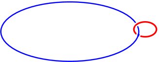
Figure 5: Geometric transitions: The branes wrap the large (blue) cycle; the flux through the Gaussian (small, red) cycle measures the brane charge. In the open-string picture the small (red) cycle has non-zero size, and the large (blue) cycle is contractible. After the geometric transition the size of the large (blue) cycle becomes zero, while the small (red) cycle becomes topologically non-trivial.

Geometric transitions appear in many systems [84, 62, 85, 86]. A classic example of such system are the brane models that break an ${\cal N}=2$ superconformal field theory down to an ${\cal N}=1$ supersymmetric field theory [62, 87]. Typically, the ${\cal N}=2$ superconformal field theory is realized on a stack of D3 branes in some Calabi-Yau compactification. One can then break the supersymmetry to ${\cal N}=1$ by introducing extra D5 branes that wrap a two-cycle. When one investigates the closed-string picture, the two cycle collapses and the dual three-cycle blows up (this is also known as a conifold transition). The D5 branes disappear and are replaced by non-trivial fluxes on the three-cycle. The resulting geometry has no more brane sources, and has a different topology than the one we started with.

Our purpose here is to see precisely how geometric transitions resolve the singularity of the zero-entropy black ring (supertube) of Section 3. Here the ring wraps a curve $y^{\mu}(\sigma)$, that is topologically an $S^{1}$ inside ${R}^{4}$. (In Fig. 6 this $S^{1}$ is depicted as a large, blue cycle.) The Gaussian cycle for this $S^{1}$ is a two-sphere around the ring (illustrated by the red small cycle in Fig. 6). If one integrates the field strengths $\Theta^{(I)}$ on the red Gaussian two-cycle one obtains the M5 brane dipole charges of the ring, $n^{I}$.

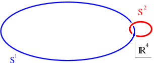
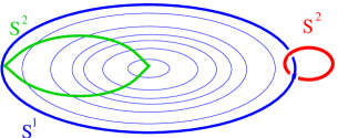
Figure 6: The geometric transition of the black ring: Before the transition the branes wrap the large (blue) $S^{1}$; the flux through the Gaussian $S^{2}$ (small, red) cycle measures the brane charge. After the transition the Gaussian $S^{2}$ (small, red) cycle is topologically non-trivial and of finite size and a new (green) $S^{2}$ appears, coming from the fact that the blue $S^{1}$ shrinks to zero so that the disk spanning the $S^{1}$ becomes an $S^{2}$. The resulting geometry has two non-trivial $S^{2}$’s and no brane sources.

After the geometric transition the large (blue) $S^{1}$ becomes of zero length, and the red $S^{2}$ becomes topologically non-trivial. Moreover, because the original topology is trivial, the curve $y^{\mu}(\sigma)$ was the boundary of a disk. When after the transition this boundary curve collapses, the disk becomes a (topologically non-trivial) two-sphere. Alternatively, one can think about this two-sphere (shown in Fig. 6 in green) as coming from having an $S^{1}$ that has zero size both at the origin of the space $r=0$ and at the location of the ring. Hence, before the transition we had a ring wrapping a curve of arbitrary shape inside ${R}^{4}$, and after the transition we have a manifold that is asymptotically ${R}^{4}$, and has two non-trivial two-spheres, and no brane sources.

Can we determine the geometry of such a manifold? If the curve has an arbitrary shape the only information about this manifold is that it is asymptotically ${R}^{4}$ and that it is hyper-Kähler, as required by supersymmetry. If the curve wrapped by the supertube has arbitrary shape, this is not enough to determine the space that will come out after the geometric transition. However, if one considers a circular supertube, the solution before the transition has a $U(1)\times U(1)$ invariance, and so one naturally expects the solution resulting from the transition should also have this invariance.

With such a high level of symmetry we do have enough information to determine what the result of the geometric transition is:
$\bullet$ By a theorem of Gibbons and Ruback [68], a hyper-Kähler manifold that has a $U(1)\times U(1)$ invariance must have a translational $U(1)$ invariance and hence, must be Gibbons-Hawking.
$\bullet$ We also know that this manifold should have two non-trivial two-cycles, and hence, as we have discussed in Section 4.1 it should have three centers.
$\bullet$ Each of these centers must have integer GH charge.
$\bullet$ The sum of the three charges must be 1, in order for the manifold to be asymptotically ${R}^{4}$.
$\bullet$ Moreover, we expect the geometric transition to be something that happens locally near the ring, and so we expect the region near the center of the ring (which is also the origin of our coordinate system) to remain the same. Hence, the GH center at the origin of the space must have charge + 1.

The conclusion of this argument is that the space that results from the geometric transition of a $U(1)\times U(1)$ invariant supertube must be a GH space with three centers, that have charges $1,~{}+Q,~{}-Q$, where $Q$ is any integer. As we have seen in Section 5.5, equation (126), if we think about ${R}^{4}$ as a trivial Gibbons-Hawking metric with $V={1\over r}$, the black ring solution of Section 3.4 has a GH center at the origin, and the ring at a certain point on the ${R}^{3}$ base of the GH space. In the “transitioned” solution, the singularity of the zero-entropy black ring is resolved by the nucleation, or “pair creation,” of two equal and oppositely charged GH points.

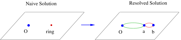
Figure 7: Geometric transition of supertube: The first diagram shows the geometry before the transition. The second shows the resolved geometry, where a pair of GH charges has nucleated at positions $a$ and $b$.

This process is depicted in Fig. 7. The nucleation of a GH pair of oppositely-charged centers blows up a pair of two-cycles. In the resolved geometry there are no more brane sources, only fluxes through the two-cycles. The charge of the solution does not come from any brane sources, but from having non-trivial fluxes over intersecting two-cycles (or “bubbles”).

Similarly, if one considers the geometric transition of multiple concentric black rings, one will nucleate one pair of GH points for each ring, resulting in a geometry with no brane sources, and with a very large number of positive and negative GH centers. As we will see, these centers are not restricted to be on a line, but can have arbitrary positions in the ${R}^{3}$ base of the GH space, as long as certain algebraic equations (discussed in Section 6.3) are satisfied.

There is one further piece of physical intuition that is extremely useful in understanding these bubbled geometries. As we have already remarked, GH points can be interpreted, from a ten-dimensional perspective, as D6 branes. Since these branes are mutually BPS, there should be no force between them. On the other hand, D6 branes of opposite charge attract one another, both gravitationally and electromagnetically. If one simply compactifies M-theory on an ambipolar GH space, one can only hold in equilibrium GH points of opposite charge at the cost of having large regions where the metric has the wrong signature and CTC’s. To eliminate these singular regions, one must hold the GH points apart by some other mechanism. In the geometries we seek, this is done by having fluxes threading the bubbles: Collapsing a bubble concentrates the energy density of the flux and increases the energy in the flux sector. Thus a flux tends to blow up a cycle. The regular, ambipolar BPS configurations that we construct come about when these two competing effects - the tendency of oppositely charged GH points to attract each other and the tendency of the fluxes to make the bubbles large - are in balance. We will see precisely how this happens in Section 6.3.

Before proceeding to construct these solutions, we should note that there are two other completely different ways of arriving at the conclusion that three-charge black hole microstates can have a base given by a GH space with negative centers.

One direction, mostly followed by Mathur, Giusto and Saxena [23, 24, 25] is to construct microstates by taking a novel extremal limit of the non-extremal five-dimensional black hole [88]. This limit produces a smooth horizonless geometries that have a GH base with two centers, of charges $N+1$ and $-N$. These geometries have a known CFT interpretation, and form a subset of the class described above. A solution that is locally identical (but differs by a global identification of charges) was also found in [26] by doing a spectral flow on a two-charge solution and extending the resulting solution to an asymptotically flat one.

The second direction, followed by Kraus and one of the present authors is to consider the four-dimensional black hole with D1-D5-KKM-P charges, when the momentum is taken to zero. The resulting naive solution for the zero-entropy four-dimensional black hole is singular, and is resolved by an intriguing mechanism: The branes that form the black hole split into two stacks, giving a non-singular solution [27]. One can then relate the black ring to a four-dimensional black hole by putting it in a Taub-NUT background, as discussed in Section 5.6 and in [58, 59, 60], and then the nucleation of a pair of oppositely-charged GH centers corresponds, from a four-dimensional point of view, to the splitting of the zero-entropy four-dimensional black hole into two stacks of branes, giving a smooth resulting solution.

Hence, we have three completely independent routes for obtaining three-charge microstates and resolving the singularity of the zero-entropy black ring, and all three routes support the same conclusion: The singularity of the zero-entropy black ring is resolved by the nucleation of GH centers of opposite charge. The solutions that result, as well as other three-charge microstate solutions, are topologically non-trivial, have no brane sources, and are smooth despite the fact that they are constructed using an ambipolar GH metric (with regions where the metric is negative-definite).

6.2 The bubbled solutions

We now proceed to construct the general form of bubbling solutions constructed using an ambipolar Gibbons-Hawking base [28, 29, 30]. In Section 4.2 we saw that the two-forms, $\Theta^{(I)}$, will be regular, self-dual, harmonic two-forms, and thus representatives of the cohomology dual to the two-cycles, provided that the $K^{I}$ have the form:

$$K^{I}~{}=~{}k^{I}_{0}~{}+~{}\sum_{j=1}^{N}\,{k_{j}^{I}\over r_{j}}\,.$$ (137)

Moreover, from (88), the flux of the two-form, $\Theta^{(I)}$, through the two-cycle $\Delta_{ij}$ is given by

$$\Pi_{ij}^{(I)}~{}=~{}\bigg{(}{k^{I}_{j}\over q_{j}}~{}-~{}{k^{I}_{i}\over q_{i}}\bigg{)}\,,\qquad 1\leq i,j\leq N\,.$$ (138)

The functions, $L_{I}$ and $M$, must similarly be chosen to ensure that the warp factors, $Z_{I}$, and the function, $\mu$, are regular as $r_{j}\to 0$. This means that we must take:

$$L^{I}~{}=~{}\ell^{I}_{0}~{}+~{}\sum_{j=1}^{N}\,{\ell_{j}^{I}\over r_{j}}\,,\quad M~{}=~{}m_{0}~{}+~{}\sum_{j=1}^{N}\,{m_{j}\over r_{j}}\,,$$ (139)

with

$$\ell_{j}^{I} ~{}=~{} -{\textstyle{1\over 2}}\displaystyle\,C_{IJK}\,{k_{j}^{J}\,k_{j}^{K}\over q_{j}}\,,\qquad j=1,\dots,N\,;$$ (140)

$$m_{j} ~{}=~{} {\textstyle{1\over 12}}\displaystyle\,C_{IJK}{k_{j}^{I}\,k_{j}^{J}\,k_{j}^{K}\over q_{j}^{2}}~{}=~{}{\textstyle{1\over 2}}\displaystyle\,{k_{j}^{1}\,k_{j}^{2}\,k_{j}^{3}\over q_{j}^{2}}\,,\qquad j=1,\dots,N\,.$$ (141)

Since we have now fixed the eight harmonic functions, all that remains is to solve for $\omega$ in equation (94). The right-hand side of (94) has two kinds of terms:

$${1\over r_{i}}\,\vec{\nabla}\,{1\over r_{j}}~{}-~{}{1\over r_{j}}\,\vec{\nabla}\,{1\over r_{i}}\qquad{\rm and}\qquad\vec{\nabla}\,{1\over r_{i}}\,.$$ (142)

Hence $\omega$ will be built from the vectors $\vec{v}_{i}$ of (84) and some new vectors, $\vec{w}_{ij}$, defined by:

$$\vec{\nabla}\times\vec{w}_{ij}~{}=~{}{1\over r_{i}}\,\vec{\nabla}\,{1\over r_{j}}~{}-~{}{1\over r_{j}}\,\vec{\nabla}\,{1\over r_{i}}\,.$$ (143)

To find a simple expression for $\vec{w}_{ij}$ it is convenient to use the coordinates outlined earlier with the $z$-axis running through $\vec{y}^{(i)}$ and $\vec{y}^{(j)}$. Indeed, choose coordinates so that $\vec{y}^{(i)}~{}=~{}(0,0,a)$ and $\vec{y}^{(j)}~{}=~{}(0,0,b)$ and one may take $a>b$. Then the explicit solutions may be written very simply:

$$w_{ij}~{}=~{}-{(x^{2}+y^{2}+(z-a)(z-b))\over(a-b)\,r_{i}\,r_{j}}\,d\phi\,.$$ (144)

This is then easy to convert to a more general system of coordinates. One can then add up all the contributions to $\omega$ from all the pairs of points.

There is, however, a more convenient basis of vector fields that may be used instead of the $w_{ij}$. Define:

$$\omega_{ij}~{}\equiv~{}w_{ij}+{\textstyle{1\over(a-b)}}\displaystyle\,\big{(}v_{i}-v_{j}+d\phi\big{)}~{}=~{}-{(x^{2}+y^{2}+(z-a+r_{i})(z-b-r_{j}))\over(a-b)\,r_{i}\,r_{j}}\,d\phi\,,$$ (145)

These vector fields then satisfy:

$$\vec{\nabla}\times\vec{\omega}_{ij}~{}=~{}{1\over r_{i}}\,\vec{\nabla}\,{1\over r_{j}}~{}-~{}{1\over r_{j}}\,\vec{\nabla}\,{1\over r_{i}}~{}+~{}{1\over r_{ij}}\,\bigg{(}\vec{\nabla}\,{1\over r_{i}}~{}-~{}\vec{\nabla}\,{1\over r_{j}}\bigg{)}\,,$$ (146)

where

$$r_{ij}~{}\equiv~{}|\vec{y}^{(i)}~{}-~{}\vec{y}^{(j)}|$$ (147)

is the distance between the $i^{\rm th}$ and $j^{\rm th}$ center in the Gibbons-Hawking metric.

We then see that the general solution for $\vec{\omega}$ may be written as:

$$\vec{\omega}~{}=~{}\sum_{i,j}^{N}\,a_{ij}\,\vec{\omega}_{ij}~{}+~{}\sum_{i}^{N}\,b_{i}\,\vec{v}_{i}\,,$$ (148)

for some constants $a_{ij}$, $b_{i}$.

The important point about the $\omega_{ij}$ is that they have no string singularities whatsoever. They can be used to solve (94) with the first set of source terms in (142), without introducing Dirac-Misner strings, but at the cost of adding new source terms of the form of the second term in (142). If there are $N$ source points, $\vec{y}^{(j)}$, then using the $w_{ij}$ suggests that there are ${1\over 2}N(N-1)$ possible string singularities associated with the axes between every pair of points $\vec{y}^{(i)}$ and $\vec{y}^{(j)}$. However, using the $\omega_{ij}$ makes it far more transparent that all the string singularities can be reduced to those associated with the second set of terms in (142) and so there are at most $N$ possible string singularities and these can be arranged to run in any direction from each of the points $\vec{y}^{(j)}$.

Finally, we note that the constant terms in (72), (137) and (139) determine the behavior of the solution at infinity. If the asymptotic geometry is Taub-NUT, all these term can be non-zero, and they correspond to combinations of the moduli. However, in order to obtain solutions that are asymptotic to five-dimensional Minkowski space, ${R}^{4,1}$, one must take $\varepsilon_{0}=0$ in (72), and $k_{0}^{I}=0$ in (137). Moreover, $\mu$ must vanish at infinity, and this fixes $m_{0}$. For simplicity we also fix the asymptotic values of the moduli that give the size of the three $T^{2}$’s, and take $Z_{I}\to 1$ as $r\to\infty$. Hence, the solutions that are asymptotic to five-dimensional Minkowski space have:

$$\varepsilon_{0}=0\,,\qquad k_{0}^{I}=0\,,\qquad l_{0}^{I}=1\,,\qquad m_{0}=-{\textstyle{1\over 2}}\displaystyle\,q_{0}^{-1}\,\sum_{j=1}^{N}\,\sum_{I=1}^{3}k_{j}^{I}\,.$$ (149)

It is straightforward to generalize these results to solutions with different asymptotics, and in particular to Taub-NUT.

6.3 The bubble equations

In Section 5.3 we examined the conditions for the absence of CTC’s and in general the following must be true globally:

$${\cal Q}~{}\geq~{}0\,,\qquad V\,Z_{I}~{}=~{}{\textstyle{1\over 2}}\displaystyle\,C_{IJK}\,K^{J}\,K^{K}~{}+~{}L_{I}\,V~{}\geq~{}0\,,\qquad I=1,2,3\,.$$ (150)

As yet, we do not know how to verify these conditions in general, but one can learn a great deal by studying the limits in which one approaches a Gibbons-Hawking point, i.e. $r_{j}\to 0$. From this one can derive some simple, physical conditions (the Bubble Equations) that in some examples ensure that (150) are satisfied globally.

To study the limit in which $r_{j}\to 0$, it is simpler to use (99) than (101). In particular, as $r_{j}\to 0$, the functions, $Z_{I}$, $\mu$ and $W$ limit to finite values while $V^{-1}$ vanishes. This means that the circle defined by $\psi$ will be a CTC unless we impose the additional condition:

$$\mu(\vec{y}=\vec{y}^{(j)})~{}=~{}0\,,\quad j=1,\dots,N\,.$$ (151)

There is also potentially another problem: The small circles in $\phi$ near $\theta=0$ or $\theta=\pi$ will be CTC’s if $\omega$ has a finite $d\phi$ component near $\theta=0$ or $\theta=\pi$. Such a finite $d\phi$ component corresponds precisely to a Dirac-Misner string in the solution and so we must make sure that $\omega$ has no such string singularities.

It turns out that these two sets of constraints are exactly the same. One can check this explicitly, but it is also rather easy to see from (91). The string singularities in $\vec{\omega}$ potentially arise from the $\vec{\nabla}(r_{j}^{-1})$ terms on the right-hand side of (91). We have already arranged that the $Z_{I}$ and $\mu$ go to finite limits at $r_{j}=0$, and the same is automatically true of $K^{I}V^{-1}$. This means that the only term on the right hand side of (91) that could, and indeed will, source a string is the $\mu\vec{\nabla}V$ term. Thus removing the string singularities is equivalent to (151).

One should note that by arranging that $\mu$, $\omega$ and $Z_{I}$ are regular one has also guaranteed that the physical Maxwell fields, $dA^{(I)}$, in (108) are regular. Furthermore, by removing the Dirac strings in $\omega$ and by requiring $\mu$ to vanish at GH points one has guaranteed that the physical flux of $dA^{(I)}$ through the cycle $\Delta_{ij}$ is still given by (88) (and (138)). This is because the extra terms, $d(Z_{I}^{-1}k)$, in (108), while canceling the singular behaviour when $V=0$, as in (109), give no further contribution in (88). Thus the fluxes, $\Pi_{ij}^{(I)}$, are well-defined and represent the true physical, magnetic flux in the five-dimensional extension of the ambipolar GH metrics.

Performing the expansion of $\mu$ using (93), (137), (139) and (141) around each Gibbons-Hawking point one finds that (151) becomes the Bubble Equations:

$$\sum_{{\scriptstyle j=1}\atop{\scriptstyle j\neq i}}^{N}\,\,\Pi^{(1)}_{ij}\,\Pi^{(2)}_{ij}\,\Pi^{(3)}_{ij}\ {q_{i}\,q_{j}\over r_{ij}}~{}=~{}-2\,\Big{(}m_{0}\,q_{i}~{}+~{}{\textstyle{1\over 2}}\displaystyle\sum_{I=1}^{3}k^{I}_{i}\Big{)}\,,$$ (152)

where $r_{ij}\equiv|\vec{y}^{(i)}-\vec{y}^{(j)}|$. One obtains the same set of equations if one collects all the Dirac string contributions to $\omega$ and sets them to zero by imposing $b_{i}=0$ in (148). If one adds together all of the bubble equations, then the left-hand side vanishes identically, and one obtains the condition on $m_{0}$ in (149). This is simply the condition $\mu\to 0$ as $r\to\infty$ and means that there is no Dirac-Misner string running out to infinity. Thus there are only $(N-1)$ independent bubble equations.

We refer to (152) as the bubble equations because they relate the flux through each bubble to the physical size of the bubble, represented by $r_{ij}$. Note that for a generic configuration, a bubble size can only be non-zero if and only if all three of the fluxes are non-zero. Thus the bubbling transition will only be generically possible for the three-charge system. We should also note that from a four-dimensional perspective these equations describe a collection of BPS stacks of branes, and are thus particular case of a collection of BPS black holes. Such configurations have been constructed in [71], and the equations that must be satisfied by the positions of the black holes are called “integrability equations” and reduce to the equations (152) when the charges are such that the five-dimensional solution is smooth.

6.4 The asymptotic charges

As in Section 3.3, one can obtain the electric charges and angular momenta of bubbled geometries by expanding $Z_{I}$ and $k$ at infinity. It is, however, more convenient to translate the asymptotics into the standard coordinates of the Gibbons-Hawking spaces. Thus, remembering that $r={1\over 4}\rho^{2}$, one has

$$Z_{I}~{}\sim~{}1~{}+~{}\,{Q_{I}\over 4\,r}~{}+~{}\dots\,,\qquad\rho\to\infty\,,$$ (153)

and from (89) one easily obtains

$$Q_{I}~{}=~{}-2\,C_{IJK}\,\sum_{j=1}^{N}\,q_{j}^{-1}\,\tilde{k}^{J}_{j}\,\tilde{k}^{K}_{j}\,,$$ (154)

where

$$\tilde{k}^{I}_{j}~{}\equiv~{}k^{I}_{j}~{}-~{}q_{j}\,N\,k_{0}^{I}\,,\qquad{\rm and}\qquad k_{0}^{I}~{}\equiv~{}{1\over N}\,\sum_{j=1}^{N}k_{j}^{I}\,.$$ (155)

Note that $\tilde{k}^{I}_{j}$ is gauge invariant under (80).

One can read off the angular momenta using an expansion like that of (42). However, it is easiest to re-cast this in terms of the Gibbons-Hawking coordinates. The flat GH metric (near infinity) has $V={1\over r}$ and making the change of variable $r={1\over 4}\rho^{2}$, one obtains the metric in spherical polar coordinates:

$$ds_{4}^{2}~{}=~{}d\rho^{2}~{}+~{}{\textstyle{1\over 4}}\displaystyle\,\rho^{2}\,(d\theta^{2}+\sin^{2}\theta\,d\phi^{2}~{}+~{}(d\psi+\cos\theta\,d\phi)^{2})\,.$$ (156)

This can be mapped to the form of (41) via the change of variable:

$$u\,e^{i\theta_{1}}~{}=~{}\rho\cos({\textstyle{1\over 2}}\displaystyle\theta)\,e^{{i\over 2}(\psi+\phi)}\,,\qquad v\,e^{i\theta_{2}}~{}=~{}\rho\sin({\textstyle{1\over 2}}\displaystyle\theta)\,e^{{i\over 2}(\psi-\phi)}\,.$$ (157)

Using this in (42) one finds that

$$k~{}\sim~{}{1\over 4\,\rho^{2}}\,\big{(}(J_{1}+J_{2})~{}+~{}(J_{1}-J_{2})\,\cos\theta\big{)}\,d\psi~{}+~{}\dots\,.$$ (158)

Thus, one can get the angular momenta from the asymptotic expansion of $g_{t\psi}$, which is given by the coefficient of $d\psi$ in the expansion of $k$, which is proportional to $\mu$. There are two types of such terms, the simple ${1\over r}$ terms and the dipole terms arising from the expansion of $V^{-1}K^{I}$. Following [29], define the dipoles

$$\vec{D}_{j}~{}\equiv~{}\,\sum_{I}\,\tilde{k}_{j}^{I}\,\vec{y}^{(j)}\,,\qquad\vec{D}~{}\equiv~{}\sum_{j=1}^{N}\,\vec{D}_{j}\,.$$ (159)

and then the expansion of $k$ takes the form (158) if one takes $\vec{D}$ to define the polar axis from which $\theta$ is measured. One then arrives at

$$J_{R}~{}\equiv~{}J_{1}+J_{2}~{}=~{}{\textstyle{4\over 3}}\displaystyle\,\,C_{IJK}\,\sum_{j=1}^{N}q_{j}^{-2}\,\tilde{k}^{I}_{j}\,\tilde{k}^{J}_{j}\,\tilde{k}^{K}_{j}\,,$$ (160)

$$J_{L}~{}\equiv~{}J_{1}-J_{2}~{}=~{}8\,\big{|}\vec{D}\big{|}\,.$$ (161)

While we have put modulus signs around $\vec{D}$ in (161), one should note that it does have a meaningful orientation, and so we will sometimes consider $\vec{J}_{L}=8\vec{D}$.

One can use the bubble equations to obtain another, rather more intuitive expression for $J_{1}-J_{2}$. One should first note that the right-hand side of the bubble equation, (152), may be written as $-\sum_{I}\tilde{k}_{i}^{I}$. Multiplying this by $\vec{y}^{(i)}$ and summing over $i$ yields:

$$\vec{J}_{L} ~{}\equiv~{} 8\,\vec{D}~{}=~{}-{\textstyle{4\over 3}}\displaystyle\,C_{IJK}\,\sum_{{\scriptstyle i,j=1}\atop{\scriptstyle j\neq i}}^{N}\,\,\Pi^{(I)}_{ij}\,\Pi^{(J)}_{ij}\,\Pi^{(K)}_{ij}\ {q_{i}\,q_{j}\,\vec{y}^{(i)}\over r_{ij}}$$ (162)

$$~{}=~{} -{\textstyle{2\over 3}}\displaystyle\,C_{IJK}\,\sum_{{\scriptstyle i,j=1}\atop{\scriptstyle j\neq i}}^{N}\,q_{i}\,q_{j}\,\Pi^{(I)}_{ij}\,\Pi^{(J)}_{ij}\,\Pi^{(K)}_{ij}\ {(\vec{y}^{(i)}-\vec{y}^{(j)})\over\big{|}\vec{y}^{(i)}-\vec{y}^{(j)}\big{|}}\,,$$

where we have used the skew symmetry $\Pi_{ij}=-\Pi_{ji}$ to obtain the second identity. This result suggests that one should define an angular momentum flux vector associated with the $ij^{\rm th}$ bubble:

$$\vec{J}_{L\,ij}~{}\equiv~{}-{\textstyle{4\over 3}}\displaystyle\,q_{i}\,q_{j}\,C_{IJK}\,\Pi^{(I)}_{ij}\,\Pi^{(J)}_{ij}\,\Pi^{(K)}_{ij}\,\hat{y}_{ij}\,,$$ (163)

where $\hat{y}_{ij}$ are unit vectors,

$$\hat{y}_{ij}~{}\equiv~{}{(\vec{y}^{(i)}-\vec{y}^{(j)})\over\big{|}\vec{y}^{(i)}-\vec{y}^{(j)}\big{|}}\,.$$ (164)

This means that the flux terms on the left-hand side of the bubble equation actually have a natural spatial direction, and once this is incorporated, it yields the contribution of the bubble to $J_{L}$.

6.5 Comments on closed time-like curves and the bubble equations

While the bubble equations are necessary to avoid CTC’s near the Gibbons-Hawking points, they are not sufficient to guarantee the absence of CTC’s globally. Indeed, there are non-trivial examples that satisfy the bubble equations and still have CTC’s. On the other hand, there are quite a number of important physical examples in which the bubble equations do guarantee the absence of CTC’s globally. For example, the simplest bubbled supertube will be discussed in Section 7.1 and it has been shown numerically in some examples that the bubble equations do indeed ensure the global absence of CTC’s. Some more complex examples that are free of CTC’s are described in Section 8.4. It is an open question as to how and when a bubbled configuration that satisfies (152) is globally free of CTC’s. In this section we will make some simple observations that suggest approaches to solving this problem.

First we need to dispel a “myth” or, more precisely, give a correct statement of an often mis-stated theorem that in a BPS solution of extremal black holes, all the black holes must have electric charges of the same sign. The physical intuition is simple: If two BPS black holes have opposite charges, then they necessarily attract both gravitationally and electromagnetically and cannot be stationary and this time dependence breaks the supersymmetry of the original BPS solutions. While this is physically correct, there is an implicit assumption that we are not going to allow physical solutions to have CTC’s, changes in metric signature, or regions with complex metrics. A simple example is to make a solution with BMPV black holes given by the harmonic function:

$$Z_{I}~{}=~{}Z~{}\equiv~{}1~{}+~{}{Q\over r_{1}}~{}-~{}{Q\over r_{2}}\,.$$ (165)

We are not advocating that solutions like this, or ones with CTC’s in general, should be taken as physically sensible. Nevertheless, this solution does satisfy all the equations of motion. The point we wish to make is that if one takes a completely standard, multi-centered BPS solution one can get lots of CTC’s or imaginary metric coefficients if one is sloppy about the relative signs of the distributed charges. For this reason, one cannot expect to take a bubbled geometry and randomly assign some flux parameters and expect to avoid CTC’s even if one has satisfied the bubble equations. Indeed, a bubbled analogue of the BMPV configuration (165) could easily satisfy the bubble equations thereby avoiding CTC’s near the Gibbons-Hawking points, only to have all sorts of pathology in between the two bubbled black holes.

There must therefore be some kind of positivity condition on the flux parameters. One suggestion might be to look at every subset, ${\cal S}$, of the Gibbons-Hawking points. To such a subset one can associate a contribution, $Q^{({\cal S})}_{I}$, to the electric charges by summing (154) only over the subset, ${\cal S}$. One could then require that the $Q^{({\cal S})}_{I}$ have the same sign for all choices of ${\cal S}$. This would exclude bubbled analogs of (165), but it might also be too stringent. It may be that one can tolerate a “mild failure” of the conditions on relative signs of electric charges if the Gibbons-Hawking points are all clustered; the danger might only occur in “classical limits” when some fluxes are very large so that the solution decomposes into two widely separated “blobs” of opposite charge.

Another natural, and possibly related condition is to remember that given $N$ Gibbons-Hawking centers, the cycles are related to the root lattice of $SU(N)$ and the dual fluxes can be labeled by the weight lattice. In this language, the obvious positivity condition is to insist that the fluxes all lie in the positive Weyl chamber of the lattice. Moreover, when there are $N_{1}$ positive and $N_{2}$ negative GH points, it may be more appropriate to think in terms of the weight lattice of a super Lie algebra, $SU(N_{1}|N_{2})$. In this context, one can rewrite $Z_{I}V$ in a rather more suggestive manner:

$$Z_{I}\,V~{}=~{}V~{}-~{}{\textstyle{1\over 4}}\displaystyle\,C_{IJK}\,\sum_{i,j=1}^{N}\,\Pi^{(J)}_{ij}\,\Pi^{(K)}_{ij}\,{q_{i}\,q_{j}\over r_{i}\,r_{j}}\,.$$ (166)

With suitable positivity conditions on the fluxes one can arrange all the terms with $q_{i}q_{j}<0$ to be positive. It is not clear why, in general, these terms dominate the terms with $q_{i}q_{j}>0$, but one can certainly verify it in examples like the one below.

Consider the situation where all the flux parameters corresponding to a given $U(1)$ are equal and positive:

$$k_{j}^{1}~{}=~{}a\,,\qquad k_{j}^{2}~{}=~{}b\,,\qquad k_{j}^{3}~{}=~{}c\,,\qquad a,b,c>0\,,\quad j=1,\dots,N\,.$$ (167)

Also suppose that $q_{j}=\pm 1$ and let $P_{\pm}$ be the subsets of integers, $j$, for which $\pm q_{j}>0$. Define

$$V_{\pm}~{}\equiv~{}\sum_{j\in P_{\pm}}{1\over r_{j}}\,.$$ (168)

Then one has

$$Z_{I}\,V~{}=~{}V~{}+~{}4\,h_{I}\,V_{+}\,V_{-}\,,$$ (169)

where $h_{1}\equiv bc$, $h_{2}\equiv ac$, $h_{3}\equiv ab$.

For this flux distribution the bubble equations reduce to:

$$8\,abc\,V_{-}(\vec{y}=\vec{y}^{(i)}) = (N-1)\,(a+b+c)\qquad{\rm for\ all}\ i\in P_{+}\,,$$ (170)

$$8\,abc\,V_{+}(\vec{y}=\vec{y}^{(j)}) = (N+1)\,(a+b+c)\qquad{\rm for\ all}\ j\in P_{-}\,.$$ (171)

Multiply the first of these equations by $r_{i}^{-1}$ and sum, and multiply the second equation by $r_{j}^{-1}$ and sum, and one obtains:

$$V_{+} = {8\,abc\over(N-1)\,(a+b+c)}\,\sum_{i\in P_{+}}\sum_{j\in P_{-}}{1\over r_{ij}}\,{1\over r_{i}}\,,$$ (172)

$$V_{-} = {8\,abc\over(N+1)\,(a+b+c)}\,\sum_{i\in P_{+}}\sum_{j\in P_{-}}{1\over r_{ij}}\,{1\over r_{j}}\,.$$ (173)

Now note that $V=V_{+}-V_{-}$ and use the foregoing expressions in (169) to obtain:

$$Z_{I}\,V = \sum_{i\in P_{+}}\sum_{j\in P_{-}}{1\over r_{i}\,r_{j}\,r_{ij}}\,\bigg{[}{8\,abc\over(a+b+c)}\Big{(}{r_{j}\over(N-1)}~{}-~{}{r_{i}\over(N+1)}\,\Big{)}$$ (174)

$$\qquad\qquad\qquad\qquad\qquad~{}+~{}4\,h_{I}\,r_{ij}\bigg{]}\,.$$

Since $a,b,c>0$ and $N>1$, one has

$${8\,abc\over(N+1)\,(a+b+c)}~{}<~{}4\,h_{I}\,,\qquad I=1,2,3\,,$$ (175)

and thus the positivity of $Z_{I}V$ follows trivially from the triangle inequality:

$$r_{j}~{}+~{}r_{ij}~{}\geq~{}r_{i}\,.$$ (176)

Note that it was relatively easy to prove positivity under the forgoing assumptions and that there was a lot of “wiggle room” in establishing the inequality. More formally, one can show that (174) is uniformly bounded below in a large compact region and so one can allow some variation of the flux parameters with $j$ and still preserve positivity. It would, of course, be very nice to know what the possible ranges of flux parameters are.

7 Microstates for black holes and black rings

Having explored the general way to construct smooth three-charge bubbling solutions that have charges and angular momenta of the same type as three-charge black holes and black rings, we now turn to exploring such solutions in greater generality. We will begin by describing several simple examples, like the simplest bubbled black ring, or a bubbled black hole made of several bubbles. We will find that when the number of bubbles is large, and the fluxes on them are generic, these solutions have the same relation between charges and angular momenta as the maximally-spinning (zero-entropy) three-charge BPS black hole ($J^{2}=N_{1}N_{5}N_{p}$). Moreover, when all the GH centers except one are in the same blob, and one GH center sits away from the blob, the solutions have the same charges, dipole charges and angular momenta as a zero-entropy, three-charge BPS black ring. Thus, to any zero-entropy black hole or any round three-charge supertube there corresponds a very large number of bubbled counterparts.

It is interesting to recall how the upper bound on the angular momentum is obtained for the BMPV black hole: One takes a solution with $J^{2}<N_{1}N_{2}N_{3}$, and imagines spinning it faster. As this happens, the closed timelike curves (CTC’s) inside the horizon get closer and closer to the horizon. When $J^{2}$ becomes larger than $N_{1}N_{2}N_{3}$, these CTC’s sit outside of the horizon and the solution has to be discarded as unphysical. A similar story happens with the black ring. What is remarkable is that this relation between the charges and angular momentum, which came from studying the solution near the horizon of the black hole and black ring, also comes out from investigating horizonless solutions with a large number of bubbles and generic fluxes. The fact that this coincidence happens both for black holes, and for black rings (as well as for BPS black holes and rings in any $U(1)^{N}$ ${\cal N}=2$, five-dimensional, ungauged supergravity), is indicative of a stronger connection between black holes and their bubbling counterparts.

Nevertheless, the fact that generic bubbling solutions correspond to zero-entropy black holes or to zero-entropy black rings means that we have only found a special corner of the microstate geometries. One might suspect, for example, that this feature comes from using a GH base space, and that obtaining microstates of positive-entropy black holes might be impossible unless one considers a more general base space. As we will see, this is not the case: We will be able to obtain microstates of black holes with $J^{2}<N_{1}N_{2}N_{3}$ by merging together zero-entropy black hole microstates and zero-entropy black ring microstates.

As we have seen in Section 3.5, unlike the merger of two BPS black holes, which is always irreversible, the merger of a BPS black hole and a BPS black ring can be reversible or irreversible, depending on the charges of the two objects. We therefore expect the merger of microstates to result in an zero-entropy microstate or a positive-entropy black-hole microstate, depending on the charges of the merging microstates. Moreover, since the merger can be achieved in a Gibbons-Hawking base, we will obtain positive-entropy black-hole microstates that have a Gibbons-Hawking base. However, as we will see in the following sections, the merger process will be full of surprises.

We will find there is a huge qualitative difference between the behaviour of the internal structure of microstates in “reversible” and “irreversible” mergers. A “reversible” merger of an zero-entropy black-hole microstate and an zero-entropy black-ring microstate produces another zero-entropy black-hole microstate. For reversible mergers we find the bubbles corresponding to the ring simply join the bubbles corresponding to the black hole, and form a bigger bubbled structure.

In an “irreversible” merger, as the ring bubbles and the black hole bubbles get closer and closer, we find that the distances between the GH points that form the black hole foam and the black ring foam also decrease. As one approaches the merger point, all the sizes in the GH base scale down to zero while preserving their relative proportions. In the limit in which the merger occurs, the solutions have $J_{1}=J_{2}<\sqrt{Q_{1}Q_{2}Q_{3}}$, and all the points have scaled down to zero size on the base. Therefore, it naively looks like the configuration is singular; however, the full physical size of the bubbles also depends on the warp factors, and taking these into account one can show that the physical size of all the bubbles that form the black hole and the black ring remains the same. The fact that the GH points get closer and closer together implies that the throat of the solution becomes deeper and deeper, and more and more similar to the throat of a BPS black hole (which is infinite).

7.1 The simplest bubbled supertube

As we have discussed in Section 6.1, we expect the solution resulting from the geometric transition of a zero-entropy black ring to contain three GH centers, of charges $q_{1}=1$, $q_{2}=-Q$ and $q_{3}=+Q$. The integral of the flux on the Gaussian two-cycle bubbled at the position of the ring gives the dipole charges of the latter, $d^{I}$. It is useful to define another physical variables $f^{I}$, measuring the fluxes through the other two-cycle:

$$d^{I}~{}\equiv~{}2\,(k_{2}^{I}~{}+~{}k_{3}^{I})\,,\qquad f_{I}~{}\equiv~{}2\,k_{1}^{I}~{}+~{}\big{(}1+{\textstyle{1\over Q}}\displaystyle\big{)}\,k_{2}^{I}~{}+~{}\big{(}1-{\textstyle{1\over Q}}\displaystyle\big{)}\,k_{3}^{I}\,.$$ (177)

Note that $d^{I}$ and $f^{I}$ are invariant under (95).

The electric charges of the bubbled tube are:

$${Q_{I}~{}=~{}C_{IJK}\,d^{J}\,f^{K}\,,}$$ (178)

and the angular momenta are:

$${J_{1}~{}=~{}-{(Q-1)\over 12\,Q}\,C_{IJK}\,{d^{I}}\,{d^{J}}\,{d^{K}}~{}+~{}{1\over 2}\,C_{IJK}\,{d^{I}}\,{d^{J}}\,{f^{K}}\,,}$$ (179)

$${J_{2}~{}=~{}{{(Q-1)}^{2}\over 24\,Q^{2}}\,C_{IJK}\,{d^{I}}\,{d^{J}}\,{d^{K}}~{}+~{}{1\over 2}\,C_{IJK}\,{f^{I}}\,{f^{J}}\,{d^{K}}\,.}$$ (180)

In particular, the angular momentum of the tube is:

$$J_{T}~{}=~{}J_{2}-J_{1}~{}=~{} {1\over 2}\,C_{IJK}\,({f^{I}}\,{f^{J}}\,{d^{K}}-{d^{I}}\,{d^{J}}\,{f^{K}})$$ (181)

$$\quad~{}+~{}\Big{(}{3\,Q^{2}-4\,Q+1\over 24\,Q^{2}}\Big{)}\,C_{IJK}\,{d^{I}}\,{d^{J}}\,{d^{K}}\,.$$

When the size of the 2-3 bubble (between GH charges $q_{2}$ and $q_{3}$) is small, this configuration can be thought of as the resolution of the singularity of the zero-entropy supertube, and has the same charges, angular momenta and size as the naive zero-entropy black ring solution. In the bubble equations, the size of the 2-3 bubble comes from a balance between the attraction of oppositely charged $GH$ points, and the fluxes that have a lot of energy when the cycle they wrap becomes very small. Hence, both when $Q$ is large and when $d$ is much smaller than $f$ the solution approaches the naive zero-entropy black ring solution

Exercise:  Verify that in the limit of large $Q$, as well as in the limit $d/f\rightarrow 0$ equations (179) and (180) match exactly the charges and angular momenta of a three-charge black ring of zero entropy.

One can also estimate, in this limit, the distance from the small 2-3 bubble to the origin of space, and find that this distance asymptotes to the radius, $R_{T}$, of the unbubbled black ring solution (as measured in the ${R}^{3}$ metric of the GH base), given by

$${J_{T}~{}=~{}4\,R_{T}\,(d^{1}+d^{2}+d^{3})\,.}$$ (182)

7.2 Microstates of many bubbles

We now consider bubbled solutions that have a large number of localized centers, and show that these solutions correspond to maximally-spinning (zero-entropy) BMPV black holes, or to maximally spinning BPS black rings [32]. The ring microstates have a blob of GH centers of zero total charge with a single GH center away from the blob while the black hole microstates have all the centers in one blob of net GH charge one. We will see that this apparently small difference can very significantly influence the solution of the bubble equations.

7.2.1 A black-hole blob

We first consider a configuration of $N$ GH centers that lie is a single “blob” and take all these centers to have roughly the same flux parameters, to leading order in $N$. To argue that such a blob corresponds to a BMPV black hole, we first need to show that $J_{1}=J_{2}$. If the overall configuration has three independent ${Z}_{2}$ reflection symmetries then this is trivial because the $\vec{D}_{j}$ in (161) will then come in equal and opposite pairs, and so one has $J_{L}=0$. More generally, for a “random” distribution the vectors $\hat{y}_{ij}$ (defined in (164)) will point in “random” directions and so the $\vec{J}_{L\,ij}$ will generically cancel one another at leading order in $N$. The only way to generate a non-zero value of $J_{L}$ is to bias the distribution such that there are more positive centers in one region and more negative ones in another. This is essentially what happens in the microstate solutions constructed and analyzed by [23, 24]. However, a single generic blob will have $J_{1}-J_{2}$ small compared to $|J_{1}|$ and $|J_{2}|$.

To compute the other properties of such a blob, we will simplify things by taking $N=2M+1$ to be odd, and assume that $q_{j}=(-1)^{j+1}$. Using the gauge invariance, we can take all of $k^{I}_{i}$ to be positive numbers, and we will assume that they have small variations about their mean value:

$${k^{I}_{j}~{}=~{}k_{0}^{I}\,(1~{}+~{}{\cal O}(1))\,,}$$ (183)

where $k_{0}^{I}$ is defined in (155). The charges are given by:

$$Q_{I} = -2\,C_{IJK}\sum_{j}q_{j}^{-1}\,(k^{J}_{j}-q_{j}Nk_{0}^{J})\,(k^{K}_{j}-q_{j}Nk_{0}^{K})$$ (184)

$$= -2\,C_{IJK}\bigg{(}\sum_{j}q_{j}^{-1}k^{J}_{j}k^{K}_{j}-Nk_{0}^{J}\sum_{j}k^{K}_{j}-Nk_{0}^{K}\sum_{j}k^{J}_{j}+N^{2}k_{0}^{J}k_{0}^{K}\sum_{j}q_{j}\bigg{)}$$

$$= 2\,C_{IJK}\Big{(}N^{2}k^{J}k^{K}-\sum_{j}k^{J}_{j}k^{K}_{j}q_{j}^{-1}\,\Big{)}$$

$$\approx 2\,C_{IJK}\big{(}N^{2}+{\cal O}(1)\big{)}\,k_{0}^{J}k_{0}^{K}$$

where we used (183) and the fact that $|q_{i}|=1$ only in the last step. In the large $N$ limit, for M theory on $T^{6}$ we have

$${Q_{1}\approx 4N^{2}k_{0}^{2}k_{0}^{3}+{\cal O}(1)\,,\quad Q_{2}\approx 4N^{2}k_{0}^{1}k_{0}^{3}+{\cal O}(1)\,,\quad Q_{3}\approx 4N^{2}_{0}k^{1}k_{0}^{3}+{\cal O}(1)\,.}$$ (185)

We can make a similar computation for the angular momenta:

$$J_{R} ~{}=~{} {\textstyle{4\over 3}}\displaystyle\,C_{IJK}\sum_{j}q_{j}^{-2}\,(k^{I}_{j}-q_{j}Nk_{0}^{I})\,(k^{J}_{j}-q_{j}Nk_{0}^{J})\,(k^{K}_{j}-q_{j}Nk_{0}^{K})$$ (186)

$$~{}=~{} {\textstyle{4\over 3}}\displaystyle\,C_{IJK}\bigg{(}\sum_{j}q_{j}^{-2}\,k^{I}_{j}k^{J}_{j}k^{K}_{j}-3Nk_{0}^{I}\sum_{j}q_{j}^{-1}\,k^{J}_{j}k^{K}_{j}$$

$$\qquad\qquad\qquad+3N^{2}k_{0}^{I}k_{0}^{J}\sum_{j}k^{K}_{j}-N^{3}k_{0}^{I}k_{0}^{J}k_{0}^{K}\sum_{j}q_{j}\bigg{)}$$

$$~{}\approx~{} {\textstyle{4\over 3}}\displaystyle\,C_{IJK}\big{(}N-3N+3N^{3}-N^{3}+{\cal O}(N)\big{)}\,k_{0}^{I}k_{0}^{J}k_{0}^{K}\,,$$

where we used the fact that, for a “well behaved” distribution of positive $k_{i}^{I}$ with $|q_{j}|=1$, one has:

$${\sum_{i}q_{i}^{-1}k^{J}_{i}k^{K}_{i}~{}=~{}\sum_{i}q_{i}k^{J}_{i}k^{K}_{i}~{}\approx~{}k_{0}^{J}k_{0}^{K}\,,\qquad\sum_{i}k^{I}_{i}k^{J}_{i}k^{K}_{i}~{}\approx~{}Nk_{0}^{I}k_{0}^{J}k_{0}^{K}\,.}$$ (187)

Therefore we simply have:

$${J_{R}~{}\approx~{}16N^{3}k_{0}^{1}k_{0}^{2}k_{0}^{3}+O(N)~{}.}$$ (188)

Since $J_{L}\approx 0$ for a generic blob at large $N$ we therefore have, at leading order:

$${J_{1}^{2}~{}\approx~{}J_{2}^{2}~{}\approx~{}{\textstyle{1\over 4}}\displaystyle\,J_{R}^{2}~{}\approx~{}Q_{1}Q_{2}Q_{3}\,,}$$ (189)

and so, in the large-$N$ limit, these microstates always correspond to a maximally spinning BMPV black hole.

Exercise:  Show that at sub-leading order in $N$ $${{J_{R}^{2}\over 4Q_{1}Q_{2}Q_{3}}~{}-~{}1\sim O\left({1\over N^{2}}\right)\,.}$$ (190)

Interestingly enough, the value of $J_{R}$ is slightly bigger than $\sqrt{4Q_{1}Q_{2}Q_{3}}$. However, this is not a problem because in the classical limit this correction vanishes. Moreover, it is possible to argue that a classical black hole with zero horizon area will receive higher-order curvature corrections, that usually increase the horizon area; hence a zero-entropy configuration will have $J_{R}$ slightly larger then the maximal classically allowed value, by an amount that vanishes in the large $N$ (classical) limit.

7.2.2 A supertube blob

The next simplest configuration to consider is one in which one starts with the blob considered above and then moves a single GH point of charge $+1$ out to a very large distance from the blob. That is, one considers a blob of total GH charge zero with a single very distant point of GH-charge $+1$. Since one now has a strongly “biased” distribution of GH charges one should now expect $J_{1}-J_{2}\neq 0$.

Again we will assume $N$ to be odd, and take the a GH charge distribution to be $q_{j}=(-1)^{j+1}$, with the distant charge being the $N^{\rm th}$ GH charge. The blob therefore has ${1\over 2}(N-1)$ points of GH charge $+1$ and ${1\over 2}(N-1)$ points of GH charge $-1$. When seen from far away one might expect this blob to resemble the three-point solution described above with $Q={1\over 2}(N-1)$. We will show that this is exactly what happens in the large-$N$ limit.

To have the $N^{\rm th}$ GH charge far from the blob means that all the two-cycles, $\Delta_{j\,N}$ must support a very large flux compared to the fluxes on the $\Delta_{ij}$ for $i,j<N$. To achieve this we therefore take:

$${k^{I}_{j}~{}=~{}a_{0}^{I}\,(1~{}+~{}{\cal O}(1))\,,\quad j=1,\dots,N-1\,,\qquad k^{I}_{N}~{}=~{}-b_{0}^{I}\,N\,.}$$ (191)

where

$${a_{0}^{I}~{}\equiv~{}{1\over(N-1)}\,\sum_{j=1}^{N-1}k_{j}^{I}\,.}$$ (192)

We also assume that $a_{0}^{I}$ and $b_{0}^{I}$ are of the same order. The fluxes of this configuration are then:

$$\Pi^{(I)}_{ij} ~{}=~{} \bigg{(}{k_{j}^{I}\over q_{j}}~{}-~{}{k_{i}^{I}\over q_{i}}\bigg{)}\,,\qquad$$ (193)

$$\Pi^{(I)}_{i\,N} ~{}=~{} -\Pi^{(I)}_{N\,i}~{}=~{}-\bigg{(}{k_{i}^{I}\over q_{i}}~{}+~{}N\,b_{0}^{I}\bigg{)}\,,\quad i,j=1,\dots,N-1\,.$$

For this configuration one has:

$$k_{0}^{I} ~{}=~{} {(N-1)\over N}\,a_{0}^{I}~{}-~{}b_{0}^{I}\,,\qquad\tilde{k}_{N}^{I}~{}=~{}-(N-1)\,a_{0}^{I}\,,$$ (194)

$$\tilde{k}^{I}_{j} ~{}=~{} k_{j}^{I}~{}+~{}q_{j}\,(N\,b_{0}^{I}-(N-1)\,a_{0}^{I})\,,\quad j=1,\dots,N-1\,.$$ (195)

Motivated by the bubbling black ring of [32] and Section 7.1, define the physical parameters:

$${d^{I}~{}\equiv~{}2\,(N-1)\,a_{0}^{I}\,,\qquad f^{I}~{}\equiv~{}(N-1)\,a_{0}^{I}-2\,N\,b_{0}^{I}\,.}$$ (196)

Keeping only the terms of leading order in $N$ in (154) and (160), one finds:

$$Q_{I} ~{}=~{} C_{IJK}d^{J}f^{K}\,,$$ (197)

$$J_{1}+J_{2} ~{}=~{} {\textstyle{1\over 2}}\displaystyle\,C_{IJK}(d^{I}d^{J}f^{K}+f^{I}f^{J}d^{K})~{}-~{}{\textstyle{1\over 24}}\displaystyle\,C_{IJK}d^{I}d^{J}d^{K}\,.$$ (198)

Since the $N^{\rm th}$ point is far from the blob, we can take $r_{iN}\approx r_{0}$ and then the $N^{\rm th}$ bubble equation reduces to:

$${{\textstyle{1\over 6}}\displaystyle\,C_{IJK}\,\sum_{j=1}^{N-1}\,\bigg{(}{k_{j}^{I}\over q_{j}}+N\,b_{0}^{I}\bigg{)}\,\bigg{(}{k_{j}^{J}\over q_{j}}+N\,b_{0}^{J}\bigg{)}\,\bigg{(}{k_{j}^{K}\over q_{j}}+N\,b_{0}^{K}\bigg{)}\,{q_{j}\over r_{0}}=(N-1)\,\sum_{I}\,a_{0}^{I}\,.}$$ (199)

To leading order in $N$ this means that the distance from the blob to the $N^{\rm th}$ point, $r_{0}$, in the GH space is given by:

$$r_{0} ~{}\approx~{} {\textstyle{1\over 2}}\displaystyle\,N^{2}\,\bigg{[}\sum_{I}\,a^{I}\bigg{]}^{-1}C_{IJK}\,a_{0}^{I}\,b_{0}^{J}\,b_{0}^{K}$$ (200)

$$~{}=~{} {\textstyle{1\over 32}}\displaystyle\,\bigg{[}\sum_{I}\,d^{I}\bigg{]}^{-1}C_{IJK}\,d^{I}\,(2f^{J}-d^{J})\,(2f^{K}-d^{K})\,.$$

Finally, considering the dipoles (159), it is evident that, to leading order in $N$, $\vec{D}$ is dominated by the contribution coming from the $N^{\rm th}$ point and that:

$$J_{1}-J_{2} ~{}=~{} 8\,|\vec{D}|~{}=~{}8\,N\,\bigg{(}\sum_{I}\,a_{0}^{I}\bigg{)}\,r_{0}~{}=~{}4\,N^{3}\,C_{IJK}\,a_{0}^{I}\,b_{0}^{J}\,b_{0}^{K}$$ (201)

$$~{}=~{} {\textstyle{1\over 8}}\displaystyle\,C_{IJK}\,d^{I}\,(2f^{J}-d^{J})\,(2f^{K}-d^{K})\,.$$ (202)

Exercise:   Verify that the angular momenta and the radius of this bubbling supertube (equations (202), (200), 197) and (198)) match those of the simplest bubbling supertube described in Section 7.1, and therefore match those of a zero-entropy black ring.

Thus, the bubbling supertube of many centers also has exactly the same size, angular momenta, charges and dipole charges as a zero-entropy black ring, and should be thought of a microstate of the later.

8 Mergers and deep microstates

As we have seen in Section 3.5, a merger of a zero-entropy black ring and a zero-entropy black hole can produce both a zero-entropy black hole (reversible merger) or a non-zero-entropy one (irreversible merger). We expect that in a similar fashion, the merger of the microstates of zero-entropy black holes and zero-entropy black rings should produce microstates of both zero-entropy and positive-entropy black holes. Since we have already constructed zero-entropy black-hole microstates, we will mainly focus on irreversible mergers and their physics. One can learn more about reversible mergers of microstates in Section 6 of [34].

Even though the original black-ring plus black-hole solution that describes the merger in Section 3.5 and [66] does not have a tri-holomorphic $U(1)$ symmetry (and thus the merger of the corresponding microstates cannot be done using a GH base), one can also study the merger of black rings and black holes by considering a $U(1)\times U(1)$ invariant solution describing a black ring with a black hole in the center. As the ring is made smaller and smaller by, for example, decreasing its angular momentum, it eventually merges into the black hole. At the point of merger, this solution is identical to the merger described in Section 3.5 with the black ring grazing the black-hole horizon. Hence this $U(1)\times U(1)$ invariant solution can be used to study mergers where the black ring grazes the black hole horizon at the point of merger. As we have seen in Section 3.5, all the reversible mergers and some of the irreversible mergers belong to this class.

In the previous section we have seen how to create bubbled solutions corresponding to a zero-entropy black ring and maximally-spinning black holes. The generic bubbled solutions with GH base have a $U(1)$ symmetry corresponding to $J_{R}\equiv J_{1}+J_{2}$ and if the GH points all lie on an axis then the solution is $U(1)\times U(1)$ invariant. We can therefore study the merger of bubbled microstates by constructing $U(1)\times U(1)$ invariant bubbling solutions describing a black ring with a black hole in the center. By changing some of the flux parameters of the solution, one can decrease the radius of the bubbling black ring and merge it into the bubbling black hole to create a larger bubbling black hole.

In this section we consider a bubbling black hole with a very large number of GH centers, sitting at the center of the simplest bubbled supertube, generated by a pair of GH points. We expect two different classes of merger solution depending upon whether the flux parameters on the bubbled black hole and bubbled black ring are parallel or not. These correspond to reversible and irreversible mergers respectively. The reversible mergers involve the GH points approaching and joining the black-hole blob to make a similar, slightly larger black-hole blob [34]. The irreversible merger is qualitatively very different and we will examine it in detail. First, however, we will establish some general results about the charges and angular momenta of the bubbled solutions that describe a bubbled black ring of two GH centers with a bubbling black-hole at the center.

8.1 Some exact results

We begin by seeing what may be deduced with no approximations whatsoever. Our purpose here is to separate all the algebraic formulae for charges and angular momenta into those associated with the black hole foam and those associated with the bubbled supertube. We will consider a system of $N$ GH points in which the first $N-2$ points will be considered to be a blob and the last two points will have $q_{N-1}=-Q$ and $q_{N}=Q$. The latter two points can then be used to define a bubbled black ring.

Let $\hat{k}_{0}^{I}$ denote the average of the flux parameters over the first $(N-2)$ points:

$${\hat{k}_{0}^{I}~{}\equiv~{}{1\over(N-2)}\,\sum_{j=1}^{N-2}\,k_{j}^{I}\,,}$$ (203)

and introduce $k$-charges that have a vanishing average over the first $(N-2)$ points:

$${\hat{k}^{I}_{j}~{}\equiv~{}k^{I}_{j}~{}-~{}(N-2)\,q_{j}\,\hat{k}_{0}^{I}\,,\qquad j=1,\dots,N-2\,.}$$ (204)

We also parameterize the last two $k^{I}$-charges in exactly the same manner as for the bubbled supertube (see equation (177)):

$$d^{I} ~{}\equiv~{} 2\,\big{(}k_{N-1}^{I}+k_{N}^{I}\big{)}\,,$$ (205)

$$f^{I} ~{}\equiv~{} 2\,(N-2)\,\hat{k}_{0}^{I}+\big{(}1+{\textstyle{1\over Q}}\displaystyle\big{)}\,k_{N-1}^{I}+\big{(}1-{\textstyle{1\over Q}}\displaystyle\big{)}\,k_{N}^{I}\,.$$

One can easily show that the charge (154) decomposes into

$${Q_{I}~{}=~{}\mathaccent 866{Q}_{I}~{}+~{}C_{IJK}\,d^{J}\,f^{K}\,,}$$ (206)

where

$${\mathaccent 866{Q}_{I}~{}\equiv~{}-2\,C_{IJK}\,\sum_{j=1}^{N-2}q_{j}^{-1}\,\hat{k}^{J}_{j}\,\hat{k}^{K}_{j}\,.}$$ (207)

The $\mathaccent 866{Q}_{I}$ are simply the charges of the black-hole blob, made of the first $(N-2)$ points. The second term in (206) is exactly the expression, (178), for the charges of a bubbled supertube with GH centers of charges $+1$, $-Q$ and $Q$ and $k$-charges $(N-2)\hat{k}_{0}^{I}$, $k_{N-1}^{I}$ and $k_{N}^{I}$, respectively. Thus the charge of this configuration decomposes exactly as if it were a black-hole blob of $(N-2)$ centers and a bubbled supertube.

There is a similar result for the angular momentum, $J_{R}$. One can easily show that:

$${J_{R}~{}=~{}\mathaccent 866{J}_{R}~{}+~{}d^{I}\,\mathaccent 866{Q}_{I}~{}+~{}j_{R}\,,}$$ (208)

where

$${\hat{J}_{R}~{}\equiv~{}{4\over 3}\,\,C_{IJK}\,\sum_{j=1}^{N-2}q_{j}^{-2}\,\hat{k}^{I}_{j}\,\hat{k}^{J}_{j}\,\hat{k}^{K}_{j}\,,}$$ (209)

and

$${j_{R}~{}\equiv~{}{\textstyle{1\over 2}}\displaystyle\,C_{IJK}\,\big{(}f^{I}f^{J}d^{K}~{}+~{}f^{I}d^{J}d^{K}\big{)}~{}-~{}{\textstyle{1\over 24}}\displaystyle\,(1-Q^{-2})\,C_{IJK}\,d^{I}d^{J}d^{K}\,.}$$ (210)

The term, $\hat{J}_{R}$, is simply the right-handed angular momentum of the black-hole blob made from $N-2$ points. The “ring” contribution to the angular momentum, $j_{R}$, agrees precisely with $J_{1}+J_{2}$ given by (179) and (180) for an isolated bubbled supertube. The cross term, $d^{I}\mathaccent 866{Q}_{I}$ is represents the interaction of the flux of the bubbled ring and the charge of the black-hole blob. This interaction term is exactly the same as that found in Section 3.5 and in [44, 55, 66] for a concentric black hole and black ring.

Thus, as far as the charges and $J_{R}$ are concerned, the complete system is behaving as though it were a black-hole blob of $(N-2)$ points interacting with a bubbled black ring defined by the points with GH charges $\pm Q$ and a single point with GH charge $+1$ replacing the black-hole blob. Note that no approximations were made in the foregoing computations, and the results are true independent of the locations of the GH centers.

To make further progress we need to make some assumptions about the configuration of the points. Suppose, for the moment, that all the GH charges lie on the $z$-axis at points $z_{i}$ with $z_{i}<z_{i+1}$. In particular, the GH charges, $-Q$ and $+Q$, are located at $z_{N-1}$ and $z_{N}$ respectively.

With this ordering of the GH points, the expression for $\vec{J}_{L}$ collapses to:

$$J_{L}~{}=~{}{\textstyle{4\over 3}}\displaystyle\,C_{IJK}\,\sum_{1\leq i<j\leq N}\,q_{i}\,q_{j}\,\Pi^{(I)}_{ij}\,\Pi^{(J)}_{ij}\,\Pi^{(K)}_{ij}\,.$$ (211)

This expression can then be separated, just as we did for $J_{R}$, into a black-hole blob component, a ring component, and interaction cross-terms. To that end, define the left-handed angular momentum of the blob to be:

$${\mathaccent 866{J}_{L}~{}=~{}{\textstyle{4\over 3}}\displaystyle\,C_{IJK}\,\sum_{1\leq i<j\leq N-2}\,q_{i}\,q_{j}\,\Pi^{(I)}_{ij}\,\Pi^{(J)}_{ij}\,\Pi^{(K)}_{ij}\,.}$$ (212)

Note that

$$\Pi^{(I)}_{ij}~{}\equiv~{}\bigg{(}{k_{j}^{I}\over q_{j}}~{}-~{}{k_{i}^{I}\over q_{i}}\bigg{)}~{}=~{}\bigg{(}{\hat{k}_{j}^{I}\over q_{j}}~{}-~{}{\hat{k}_{i}^{I}\over q_{i}}\bigg{)}\,,\qquad 1\leq i,j\leq N-2\,,$$ (213)

and so this only depends upon the fluxes in the blob.

The remaining terms in (211) may then be written in terms of $\hat{k}_{j}^{I}$, $d^{I}$ and $f^{I}$ defined in (204) and (205). In particular, there are terms that depend only upon $d^{I}$ and $f^{I}$, and then there are terms that are linear, quadratic and cubic in $\hat{k}_{j}^{I}$ (and depend upon $d^{I}$ and $f^{I}$). The linear terms vanish because $\sum_{j=1}^{N-2}\hat{k}_{j}^{I}\equiv 0$, the quadratic terms assemble into $\mathaccent 866{Q}_{I}$ of (207) and the cubic terms assemble into $\hat{J}_{R}$ of (209). The terms proportional to (209) cancel between the terms with $j=N-1$ and $j=N$, and one is left with:

$${J_{L}~{}=~{}\mathaccent 866{J}_{L}~{}-~{}d^{I}\,\mathaccent 866{Q}_{I}~{}+~{}j_{L}\,,}$$ (214)

where $j_{L}$ is precisely the angular momentum, $J_{T}$, of the tube:

$${j_{L}~{}\equiv~{}{\textstyle{1\over 2}}\displaystyle\,C_{IJK}\,\big{(}d^{I}f^{J}f^{K}~{}-~{}f^{I}d^{J}d^{K}\big{)}~{}+~{}\Big{(}{3\,Q^{2}-4\,Q+1\over 24\,Q^{2}}\Big{)}\,C_{IJK}\,d^{I}d^{J}d^{K}\,.}$$ (215)

Observe that (210) and (215) are exactly the angular momenta of a simple bubbled ring, (179) and (180). Again we see the cross-term from the interaction of the ring dipoles and the electric charge of the blob. Indeed, combining (208) and (214), we obtain:

$${J_{1}~{}=~{}\mathaccent 866{J}_{1}~{}+~{}j_{1}\,,\qquad J_{2}~{}=~{}\mathaccent 866{J}_{2}~{}+~{}j_{2}~{}-~{}d^{I}\,\mathaccent 866{Q}_{I}\,,}$$ (216)

which is exactly how the angular momenta of the classical ring-hole solution in Section 3.5 decomposed. In particular, the term coming from the interaction of the ring dipole moment with the black hole charge only contributes to $J_{2}$.

Exercise:  Check the decompositions (207), (209) and (214).

The results obtained above are independent of whether the blob of $N-2$ points is a BMPV black-hole blob, or a more generic configuration. However, to study mergers we now take the blob to be a black-hole microstate, with $\mathaccent 866{J}_{L}~{}=~{}0$. The end result of the merger process is also a BMPV black hole microstate, and so $J_{L}~{}=~{}0$. Therefore, the exact merger condition is simply:

$$\Omega \equiv {\textstyle{1\over 2}}\displaystyle\,C_{IJK}\,\big{(}d^{I}f^{J}f^{K}-f^{I}d^{J}d^{K}\big{)}+\Big{(}{3\,Q^{2}-4\,Q+1\over 24\,Q^{2}}\Big{)}\,C_{IJK}\,d^{I}d^{J}d^{K}-d^{I}\,\mathaccent 866{Q}_{I}$$ (217)

$$= 0\,.$$

Using (181), this may be written:

$${J_{T}~{}-~{}d^{I}\,\mathaccent 866{Q}_{I}~{}=~{}0\,,}$$ (218)

which is precisely the condition obtained in Section 3.5 and [66] for a classical black ring to merge with a black hole at its equator.

One should note that the argument that led to the expressions (214) and (215) for $J_{L}$, and to the exact merger condition, (217), apply far more generally. In particular we only needed the fact that the unit vectors, $\hat{y}_{ij}$, defined in (164), are all parallel for $j=N-1$ and $j=N$. This is approximately true in many contexts, and most particularly if the line between the $(N-1)^{\rm th}$ and $N^{\rm th}$ points runs through the blob and the width of the blob is small compared to the distance to the two exceptional points.

One should also not be surprised by the generality of the result in equation (215). The angular momentum, $J_{T}$, is an intrinsic property of a black ring, and hence for a zero-entropy black ring, $J_{T}$ can only depend on the $d$’s and $f$’s, and cannot depend on the black hole charges (that is, the $\hat{k}_{j}^{I}$). Therefore, we could have obtained (215) by simply setting the black hole charge to zero, and then reading off $J_{T}$ from the bubbling black ring solution of Section 7.1. Hence, one should think about the expression of $J_{T}$ in (181) as a universal relation between intrinsic properties of the bubbled ring: $J_{T},d^{I}$ and $f^{I}$.

8.2 Some simple approximations

We now return to a general distribution of GH points, but we will assume that the two “black ring points” (the $(N-1)^{\rm th}$ and $N^{\rm th}$ points) are close together but very far from the black-hole blob of the remaining $(N-2)$ points. Set up coordinates in the geometric center of the black-hole blob, i.e. choose the origin so that

$${\sum_{i=1}^{N-2}\,\vec{r}_{i}~{}=~{}0\,.}$$ (219)

Let $r_{0}\equiv|\vec{r}_{N-1}|$ be the distance from the geometric center of the blob to the first exceptional point, and let $\hat{r}_{0}$ be the the unit vector in that direction. The vector, $\vec{\Delta}\equiv\vec{r}_{N}-\vec{r}_{N-1}$, defines the width of the ring. We will assume that the magnitudes $\Delta\equiv|\vec{\Delta}|$ and $r_{j}\equiv|\vec{r}_{j}|$ are small compared to $r_{0}$. We will also need the first terms of the multipole expansions:

$${1\over|\vec{r}_{N-1}-\vec{r}_{j}|} ~{}=~{} {1\over r_{0}}~{}+~{}{\vec{r}_{j}\cdot\hat{r}_{0}\over r_{0}^{2}}~{}+~{}\dots$$ (220)

$${1\over|\vec{r}_{N}-\vec{r}_{j}|} ~{}=~{} {1\over r_{0}}~{}+~{}{(\vec{r}_{j}-\vec{\Delta})\cdot\hat{r}_{0}\over r_{0}^{2}}~{}+~{}\dots\,.$$ (221)

For simplicity, we will also assume that the two black-ring points (we will also call these points “exceptional points”) are co-linear with the origin so that

$${r_{N}~{}\equiv~{}|\vec{r}_{N}|~{}=~{}r_{0}+\Delta\,.}$$ (222)

The last two bubble equations are then:

$${{\gamma\over\Delta}~{}-~{}\sum_{j=1}^{N-2}\,{q_{j}\,\alpha_{j}\over|\vec{r}_{N}-\vec{r}_{j}|}~{}=~{}\sum_{I}\,\big{(}N\,Q\,k^{I}_{0}-k_{N}^{I}\big{)}\,,}$$ (223)

$${-{\gamma\over\Delta}~{}+~{}\sum_{j=1}^{N-2}\,{q_{j}\,\beta_{j}\over|\vec{r}_{N-1}-\vec{r}_{j}|}~{}=~{}-\sum_{I}\,\big{(}N\,Q\,k^{I}_{0}+k_{N-1}^{I}\big{)}\,}$$ (224)

where $k^{I}_{0}$ is given in (155) and

$$\alpha_{j} \equiv {\textstyle{1\over 6}}\displaystyle\,Q\,C_{IJK}\,\Pi_{j\,N}^{(I)}\,\Pi_{j\,N}^{(J)}\,\Pi_{j\,N}^{(K)}$$ (225)

$$= {\textstyle{1\over 6}}\displaystyle\,Q\,C_{IJK}\,\bigg{(}{k_{N}^{I}\over Q}-{k_{j}^{I}\over q_{j}}\bigg{)}\,\bigg{(}{k_{N}^{J}\over Q}-{k_{j}^{J}\over q_{j}}\bigg{)}\,\bigg{(}{k_{N}^{K}\over Q}-{k_{j}^{K}\over q_{j}}\bigg{)}\,,$$ (226)

$$\beta_{j} \equiv {\textstyle{1\over 6}}\displaystyle\,Q\,C_{IJK}\,\Pi_{j\,(N-1)}^{(I)}\,\Pi_{j\,(N-1)}^{(J)}\,\Pi_{j\,(N-1)}^{(K)}$$ (227)

$$= -{\textstyle{1\over 6}}\displaystyle\,Q\,C_{IJK}\,\bigg{(}{k_{N-1}^{I}\over Q}+{k_{j}^{I}\over q_{j}}\bigg{)}\,\bigg{(}{k_{N-1}^{J}\over Q}+{k_{j}^{J}\over q_{j}}\bigg{)}\,\bigg{(}{k_{N-1}^{K}\over Q}+{k_{j}^{K}\over q_{j}}\bigg{)}\,,$$ (228)

$${\gamma~{}\equiv~{}{\textstyle{1\over 6}}\displaystyle\,Q^{2}\,C_{IJK}\,\Pi_{(N-1)\,N}^{(I)}\,\Pi_{(N-1)\,N}^{(J)}\,\Pi_{(N-1)\,N}^{(K)}~{}=~{}{\textstyle{1\over 48}}\displaystyle\,Q^{-1}\,C_{IJK}\,d^{I}\,d^{J}\,d^{K}\,.}$$ (229)

It is also convenient to introduce

$${\alpha_{0}~{}\equiv~{}\sum_{j=1}^{N-2}\,q_{j}\,\alpha_{j}\,,\qquad\beta_{0}~{}\equiv~{}\sum_{j=1}^{N-2}\,q_{j}\,\beta_{j}\,.}$$ (230)

If one adds (223) and (224) then the terms involving $\gamma$ cancel and using (221) one then obtains:

$${\sum_{j=1}^{N-2}\,q_{j}\,\bigg{[}\,\alpha_{j}\,\bigg{(}{1\over r_{0}}+{(\vec{r}_{j}-\vec{\Delta})\cdot\hat{r}_{0}\over r_{0}^{2}}\bigg{)}~{}-~{}\beta_{j}\,\bigg{(}{1\over r_{0}}+{\vec{r}_{j}\cdot\hat{r}_{0}\over r_{0}^{2}}\bigg{)}\,\bigg{]}~{}=~{}{\textstyle{1\over 2}}\displaystyle\,\sum_{I}\,d^{I}\,.}$$ (231)

One now needs to perform the expansions with some care. Introduce the flux vector:

$${X^{I}~{}\equiv~{}2\,f^{I}-d^{I}-4\,(N-2)\,\hat{k}_{0}^{I}\,,}$$ (232)

and note that the fluxes between the blob and ring points are given by:

$$\Pi^{(I)}_{j\,(N-1)} ~{}=~{} -{\textstyle{1\over 4}}\displaystyle\,\big{[}\,X^{I}+Q^{-1}\,d^{I}+4\,q_{j}^{-1}\,k_{j}^{I}\,\big{]}\,,$$ (233)

$$\Pi^{(I)}_{j\,N} ~{}=~{} -{\textstyle{1\over 4}}\displaystyle\,\big{[}\,X^{I}-Q^{-1}\,d^{I}+4\,q_{j}^{-1}\,k_{j}^{I}\,\big{]}\,.$$ (234)

In particular, the difference of these fluxes is simply the flux through the two-cycle running between the two ring points:

$${\Pi^{(I)}_{j\,N}~{}-~{}\Pi^{(I)}_{j\,(N-1)}~{}=~{}{d^{I}\over 2\,Q}~{}=~{}\Pi^{(I)}_{(N-1)\,N}\,.}$$ (235)

For the ring to be far from the black hole, the fluxes $\Pi^{(I)}_{j\,(N-1)}$ and $\Pi^{(I)}_{j\,N}$ must be large. For the ring to be thin ($\Delta\ll r_{0}$), these fluxes must be of similar order, or $\Pi^{(I)}_{(N-1)\,N}$ should be small. Hence we are assuming that ${d^{I}\over 2Q}$ is small compared to $X^{I}$. We are also going to want the black hole and the black ring to have similar charges and angular momenta, $J_{R}$, and one of the ways of achieving this is to make $f^{I}$, $d^{I}$ and $N\hat{k}_{0}^{I}$ of roughly the same order.

Given this, the leading order terms in (231) become:

$${\sum_{j=1}^{N-2}\,q_{j}\,\bigg{[}\,{(\alpha_{j}-\beta_{j})\over r_{0}}~{}-~{}\alpha_{j}\,{\Delta\over r_{0}^{2}}\,\bigg{]}~{}=~{}{\textstyle{1\over 2}}\displaystyle\,\sum_{I}\,d^{I}\,.}$$ (236)

One can then determine the ring width, $\Delta$, using (223) or (224). In particular, when the ring width is small while the ring radius is large, the left-hand side of each of these equations is the difference of two very large numbers of similar magnitude. To leading order we may therefore neglect the right-hand sides and use the leading monopole term to obtain:

$${\beta_{0}\,{\Delta\over r_{0}}~{}\approx~{}\alpha_{0}\,{\Delta\over r_{0}}~{}=~{}\bigg{[}\,\sum_{j=1}^{N-2}\,q_{j}\,\alpha_{j}\,\bigg{]}\,{\Delta\over r_{0}}~{}\approx~{}\gamma\,,}$$ (237)

and hence (231) becomes:

$${-\gamma~{}+~{}\sum_{j=1}^{N-2}\,q_{j}\,(\alpha_{j}-\beta_{j})~{}\approx~{}\bigg{[}\,{\textstyle{1\over 2}}\displaystyle\,\sum_{I}\,d^{I}\,\bigg{]}\,r_{0}\,.}$$ (238)

Using the explicit expressions for $\alpha_{j},\beta_{j}$ and $\gamma$, one then finds:

$$r_{0}~{}\approx \bigg{[}4\,\sum_{I}\,d^{I}\bigg{]}^{-1}\bigg{[}\,{\textstyle{1\over 2}}\displaystyle\,C_{IJK}\,(d^{I}f^{J}f^{K}-f^{I}d^{J}d^{K})$$ (239)

$$+ \bigg{(}{3\,Q^{2}-4\,Q+1\over 24\,Q^{2}}\bigg{)}\,C_{IJK}\,d^{I}d^{J}d^{K}~{}-~{}d^{I}\mathaccent 866{Q}_{I}\,\bigg{]}\,.$$

This is exactly the same as the formula for the tube radius that one obtains from (182) and (181). Note also that we have:

$${r_{0}~{}\approx~{}\Big{[}4\,\sum_{I}\,d^{I}\Big{]}^{-1}\big{[}\,j_{L}~{}-~{}d^{I}\mathaccent 866{Q}_{I}\,\big{]}\,,}$$ (240)

where $j_{L}$ the angular momentum of the supertube (214). In making the comparison to the results of Section 3.5 recall that for a black ring with a black hole exactly in the center, the embedding radius in the standard, flat ${R}^{4}$ metric is given by:

$${R^{2}~{}=~{}{l_{p}^{6}\over L^{4}}\,\,\Big{[}\sum d^{I}\Big{]}^{-1}\,\Big{(}J_{T}~{}-~{}d^{I}\mathaccent 866{Q}_{I}\Big{)}\,.}$$ (241)

The transformation between a flat ${R}^{4}$ and the GH metric with $V={1\over r}$ involves setting $r={1\over 4}\rho^{2}$, and this leads to the relation $R^{2}=4R_{T}$. We therefore have complete consistency with the classical merger result.

Note that the classical merger condition is simply $r_{0}\to 0$, which is, of course, very natural. This might, at first, seem to fall outside the validity of our approximation, however we will see in the next section that for irreversible mergers one does indeed maintain $\Delta,r_{j}\ll r_{0}$ in the limit $r_{0}\to 0$. Reversible mergers cannot however be described in this approximation, and have to be analyzed numerically.

8.3 Irreversible mergers and scaling solutions

All the results we have obtained in Sections 8.1 and 8.2 apply equally to reversible and irreversible mergers. However, since our main purpose is to obtain microstates of a BPS back hole with classically large horizon area, we now focus on irreversible mergers.

We will show that an irreversible merger occurs in such a manner that the ring radius, $r_{0}$, the ring width, $\Delta$, and a typical separation of points within the black-hole blob all limit to zero while their ratios all limit to finite values. We will call these scaling solutions, or scaling mergers. As the merger progresses, the throat of the solution becomes deeper and deeper, and corresponding redshift becomes larger and larger. The resulting microstates have a very deep throat, and will be called “deep microstates.”

Using the solution constructed in the previous sections, we begin decreasing the radius of the bubbled ring, $r_{0}$, by decreasing some of its flux parameters. We take all the flux parameters of the $(N-2)$ points in the blob to be parallel:

$${k_{j}^{I}~{}=~{}\hat{k}_{0}^{I}~{}=~{}k^{I}\,,\qquad j~{}=~{}1,\dots,N-2\,,}$$ (242)

Further assume that all the GH charges in the black-hole blob obey $q_{j}=(-1)^{j+1}$, $j=1,\dots,N-2$. We therefore have

$$\mathaccent 866{Q}_{I} ~{}=~{} 2\,(N-1)(N-3)\,C_{IJK}\,k^{J}k^{K}\,,$$ (243)

$$\mathaccent 866{J}_{R} ~{}=~{} {\textstyle{8\over 3}}\displaystyle\,(N-1)(N-2)(N-3)\,C_{IJK}\,k^{I}k^{J}k^{K}\,.$$

Define:

$${\mu_{i}~{}\equiv~{}{\textstyle{1\over 6}}\displaystyle\,(N-2-q_{i})^{-1}\,C_{IJK}\,\sum_{{\scriptstyle j=1}\atop{\scriptstyle j\neq i}}^{N-2}\,\,\Pi^{(I)}_{ij}\,\Pi^{(J)}_{ij}\,\Pi^{(K)}_{ij}\ {q_{j}\over r_{ij}}\,,}$$ (244)

then the bubble equations for this blob in isolation (i.e. with no additional bubbles, black holes or rings) are simply:

$${\mu_{i}~{}=~{}\sum_{I=1}^{3}\,k^{I}\,,}$$ (245)

More generally, in any solution satisfying (242), if one finds a blob in which the $\mu_{i}$ are all equal to the same constant, $\mu_{0}$, then the GH points in the blob must all be arranged in the same way as an isolated black hole, but with all the positions scaled by $\mu_{0}^{-1}\big{(}\sum_{I=1}^{3}\,k^{I}\big{)}$.

Now consider the full set of $N$ points with $\Delta,r_{j}\ll r_{0}$. In Section 8.2 we solved the last two bubble equations and determined $\Delta$ and $r_{0}$ in terms of the flux parameters. The remaining bubble equations are then:

$${(N-2-q_{i})\,\mu_{i}+{\alpha_{i}\over|\vec{r}_{N}-\vec{r}_{i}|}-{\beta_{i}\over|\vec{r}_{(N-1)}-\vec{r}_{i}|}~{}=~{}\sum_{I=1}^{3}\,\big{(}(N-2-q_{i})\,k^{I}+{d^{I}\over 2}\big{)}\,,}$$ (246)

for $i=1,\dots,N-2$. Once again we use the multipole expansion in these equations:

$${(N-2-q_{i})\,\mu_{i}~{}+~{}{(\alpha_{i}-\beta_{i})\over r_{0}}~{}-~{}{\alpha_{i}\,\Delta\over r_{0}^{2}}~{}=~{}\sum_{I=1}^{3}\,\big{(}(N-2-q_{i})\,k^{I}+{d^{I}\over 2}\big{)}\,,}$$ (247)

It is elementary to show that:

$${\alpha_{i}-\beta_{i}~{}=~{}{\textstyle{1\over 8}}\displaystyle\,(j_{L}-d^{I}\,\mathaccent 866{Q}_{I})~{}+~{}\gamma~{}-~{}{\textstyle{1\over 8}}\displaystyle\,(N-2-q_{i})\,C_{IJK}\,d^{I}\,k^{J}\,X^{K}\,,}$$ (248)

where $X^{I}$ is defined in (232). If one now uses this identity, along with (237) and (240) in (247) one obtains:

$$(N-2-q_{i})\,\mu_{i} ~{}-~{} {1\over r_{0}}\,C_{IJK}\,\Big{[}{\textstyle{1\over 8}}\displaystyle\,(N-2-q_{i})\,d^{I}\,k^{J}\,X^{K}~{}-~{}\Big{(}1-{\alpha_{i}\over\alpha_{0}}\Big{)}\,\gamma\Big{]}$$ (249)

$$~{}\approx~{} (N-2-q_{i})\,\sum_{I=1}^{3}\,k^{I}\,.$$

Finally, note that:

$${\alpha_{0}-\alpha_{i}~{}=~{}Q\,(N-2-q_{i})\,C_{IJK}\,\big{[}{\textstyle{1\over 32}}\displaystyle(X^{I}-{\textstyle{1\over Q}}\displaystyle d^{I})\,(X^{J}-{\textstyle{1\over Q}}\displaystyle d^{J})\,k^{K}~{}+~{}{\textstyle{1\over 6}}\displaystyle\,k^{I}\,k^{J}\,k^{K}\big{]}\,,}$$ (250)

and so the bubble equations (246) reduce to:

$$\mu_{i} \approx \Big{(}\sum_{I=1}^{3}\,k^{I}\Big{)}~{}+~{}{1\over r_{0}}\,C_{IJK}\,\Big{[}{\textstyle{1\over 8}}\displaystyle\,d^{I}\,k^{J}\,X^{K}$$ (251)

$$\qquad\qquad~{}-~{}\alpha_{0}^{-1}\,Q\,\gamma\,\big{(}{\textstyle{1\over 32}}\displaystyle\,(X^{I}-{\textstyle{1\over Q}}\displaystyle d^{I})\,(X^{J}-{\textstyle{1\over Q}}\displaystyle d^{J})\,k^{K}~{}+~{}{\textstyle{1\over 6}}\displaystyle\,k^{I}\,k^{J}\,k^{K}\big{)}\,\Big{]}$$

$$\approx \Big{(}\sum_{I=1}^{3}\,k^{I}\Big{)}~{}+~{}{1\over r_{0}}\,C_{IJK}\,\Big{[}{\textstyle{1\over 8}}\displaystyle\,d^{I}\,k^{J}\,X^{K}$$

$$\qquad\qquad\qquad\qquad\qquad-~{}\alpha_{0}^{-1}\,Q\,\gamma\,\big{(}{\textstyle{1\over 32}}\displaystyle\,X^{I}\,X^{J}\,k^{K}+{\textstyle{1\over 6}}\displaystyle\,k^{I}\,k^{J}\,k^{K}\big{)}\,\Big{]}\,,$$ (252)

since we are assuming $X^{I}$ is large compared to $Q^{-1}d^{I}$.

Observe that the right-hand side of (251) is independent of $i$, which means that the first $(N-2)$ GH points satisfy a scaled version of the equations (245) for a isolated, bubbled black hole. Indeed, if $\vec{r}_{i}^{BH}$ are the positions of a set of GH points satisfying (245) then we can solve (251) by scaling the black hole solution, $\vec{r}_{i}=\lambda^{-1}\vec{r}_{i}^{BH}$, where the scale factor is given by:

$$\lambda ~{}\approx~{} 1~{}+~{}{1\over r_{0}}\,\Big{(}\sum_{I=1}^{3}\,k^{I}\Big{)}^{-1}\,C_{IJK}\,\Big{[}{\textstyle{1\over 8}}\displaystyle\,d^{I}\,k^{J}\,X^{K}$$ (253)

$$\qquad\qquad~{}-~{}\alpha_{0}^{-1}\,Q\,\gamma\,\big{(}{\textstyle{1\over 32}}\displaystyle\,X^{I}\,X^{J}\,k^{K}~{}+~{}{\textstyle{1\over 6}}\displaystyle\,k^{I}\,k^{J}\,k^{K}\big{)}\,\Big{]}\,.$$

Notice that as one approaches the critical “merger” value, at which $\Omega=j_{L}-d^{I}\,\mathaccent 866{Q}_{I}=0$, (253) implies that the distance, $r_{0}$, must also scale as $\lambda^{-1}$. Therefore the merger process will typically involve sending $r_{0}\to 0$ while respecting the assumptions made in our approximations ($\Delta,r_{i}\ll r_{0}$). The result will be a “scaling solution” in which all distances in the GH base are vanishing while preserving their relative sizes.

In [34] this picture of the generic merger process was verified by making quite a number of numerical computations; we urge the curious reader to refer to that paper for more details. In Section 8.4 we will only present one very simple scaling solution, which illustrates the physics of these mergers.

An important exception to the foregoing analysis arises when the term proportional to $r_{0}^{-1}$ in (251) vanishes to leading order. In particular, this happens if we violate one of the assumptions of our analysis, namely, if one has:

$${X^{I}~{}\equiv~{}2\,f^{I}-d^{I}-4\,(N-2)\,k^{I}~{}\approx~{}0\,,}$$ (254)

to leading order order in $Q^{-1}d^{I}$. If $X^{I}$ vanishes one can see that, to leading order, the merger condition is satisfied:

$$\Omega ~{}\equiv~{} j_{L}-d^{I}\,\mathaccent 866{Q}_{I}$$

$$~{}=~{} {\textstyle{1\over 8}}\displaystyle\,C_{IJK}\,d^{I}\,\big{[}X^{J}X^{K}-{\textstyle{1\over 3}}\displaystyle\,Q^{-2}\,(4\,Q-1)\,d^{J}d^{K}-16\,k^{J}k^{K}\big{]}$$

$$~{}\approx~{} 0\,,$$

and so one must have $r_{0}\to 0$. However, the foregoing analysis is no longer valid, and so the merger will not necessarily result in a scaling solution.

An important example of this occurs when $k^{I}$, $d^{I}$ and $f^{I}$ are all parallel:

$${k^{I}~{}=~{}k\,u^{I}\,,\qquad d^{I}~{}=~{}d\,u^{I}\,,\qquad f^{I}~{}=~{}f\,u^{I}\,,}$$ (256)

for some fixed $u^{I}$. Then the merger condition (8.3) is satisfied to leading order, only when $X\equiv(2\,f-d-4\,(N-2)\,k)$ vanishes.

For non-parallel fluxes it is possible to satisfy the merger condition, (8.3), while keeping $X^{I}$ large, and the result is a scaling solution.

Even if it looks like irreversible mergers progress until the final size on the base vanishes, this is an artifact of working in a classical limit an ignoring the quantization of the fluxes. After taking this into account we can see from (251) that $r_{0}$ cannot be taken continuously to zero because the $d^{I},f^{I},X^{I}$ and $k^{I}$ are integers of half-integers. Hence, the final result of an irreversible merger is a microstate of a high, but finite, redshift and whose throat only becomes infinite in the classical limit.

In order to find the maximum depth of the throat, one has to find the smallest allowed value for the size of the ensemble of GH points in the ${R}^{3}$ base of the GH space. During the irreversible merger all the distances scale, the size of the ensemble of points will be approximately equal to the distance between the ring blob and the black hole blob, which is given by (240). Since $j_{L}-d^{I}\mathaccent 866{Q}_{I}$ is quantized, the minimal size of the ensemble of GH points is given by:

$${r|_{\rm min}\approx{1\over d^{1}+d^{2}+d^{3}}\,.}$$ (257)

More generally, in the scaling limit, the GH size of a solution with left-moving angular momentum $J_{L}$ is

$${r|_{\rm min}\approx{J_{L}\over d^{1}+d^{2}+d^{3}}\,.}$$ (258)

Since the $d^{I}$ scale like the square-roots of the ring charges, we can see that in the classical limit, $r|_{\rm min}$ becomes zero and the throat becomes infinite.

8.4 Numerical results for a simple merger

Given that most of the numerical investigations and most of the derivations we have discussed above use black hole microstate made from a very large number of points, it is quite hard to illustrate explicitly the details of a microstate merger.

To do this, it is much more pedagogical to investigate a black hole microstate that is made from three points, of GH charges $-n$, $2n+1$, and $-n$, and its merger with the black ring microstate of GH charges $-Q$ and $+Q$. This black-hole microstate can be obtained by redistributing the position of the GH points inside the black-hole blob considered in Section 8.3, putting all the $+1$ charges together and putting half of the $-1$ charges together on one side of the positive center and the other half on the other side

We consider a configuration with 5 GH centers of charges

$${q_{1}=-12,~{}q_{2}=25,~{}q_{3}=-12,~{}q_{4}=-20,~{}q_{5}=20~{}.}$$ (259)

The first three points give the black-hole “blob,” which can be thought as coming from a blob of $N-2=49$ points upon redistributing the GH points as described above; the $k^{I}$ parameters of the black hole points are

$${k_{1}^{I}=q_{1}\hat{k}_{0}^{I},~{}k_{2}^{I}=q_{2}\hat{k}_{0}^{I},~{}k_{3}^{I}=q_{3}\hat{k}_{0}^{I}~{},}$$ (260)

where $\hat{k}_{0}^{I}$ is the average of the $k^{I}$ over the black-hole points, defined in (203). To merge the ring and the black hole microstates we have varied $\hat{k}_{0}^{2}$ keeping $\hat{k}_{0}^{1}$ and $\hat{k}_{0}^{3}$ fixed:

$${\hat{k}_{0}^{1}={5\over 2},~{}\hat{k}_{0}^{3}={1\over 3},~{}}$$ (261)

We have also kept fixed the ring parameters $f^{I}$ and $d^{I}$:

$${d^{1}=100,~{}d^{2}=130,~{}d^{3}=80,~{}f^{1}=f^{2}=160,~{}f^{3}=350}$$ (262)

The relation between these parameters and the $k^{I}$ of the ring is given in (205), where $N-2$ (the sum of $|q_{i}|$ for the black hole points) is now $|q_{1}|+|q_{2}|+|q_{3}|=49$ .

  $$\hat{k}^{2}_{0} x_{4}-x_{3} {x_{4}-x_{3}\over x_{2}-x_{1}} {x_{2}-x_{1}\over x_{3}-x_{2}} {x_{2}-x_{1}\over x_{5}-x_{4}} J_{L} {\cal{H}}$$                      0 3.0833  175.5 2225 1.001 2.987  215983 .275  1 3.1667 23.8 2069 1.001 3.215 29316 .278  2 3.175 8.65 2054 1.001 3.239 10650 .279  3 3.1775 4.10 2049 1.001 3.246 5050 .279  4 3.178 3.19 2048 1.001 3.248 3930 .279  5 3.17833 2.59 2048 1.001 3.249 3183 .279  6 3.17867 1.98 2047 1.001 3.250 2437 .279  7 3.1795 .463 2046 1.001 3.252 570 .279  8  3.17967 .160 2045 1.001 3.253 197 .279  

Table 1: Distances between points in the scaling regime. The parameter ${\cal H}\equiv{Q_{1}Q_{2}Q_{3}-J_{R}^{2}/4\over Q_{1}Q_{2}Q_{3}}$ measures how far away the angular momentum of the resulting solution is from the angular momentum of the maximally-spinning black hole with identical charges. The value of $\hat{k}_{0}^{2}$ is varied to produce the merger, and the other parameters of the configuration are kept fixed: $Q=20,~{}q_{1}=q_{3}=-12,~{}q_{2}=25,~{}\hat{k}_{0}^{1}={5\over 2},~{}\hat{k}_{0}^{3}={1\over 3},~{}d^{1}=100,~{}d^{2}=130,~{}d^{3}=80,~{}f^{1}=f^{2}=160,~{}f^{3}=350$. Both the charges and $J_{R}$ remain approximately constant, with $J_{R}\approx 3.53\times 10^{7}$

The charges and $J_{R}$ angular momentum of the solutions are approximately

$${Q_{1}\approx 68.4\times 10^{3},~{}Q_{2}\approx 55.8\times 10^{3},~{}Q_{3}\approx 112.8\times 10^{3},~{}J_{R}\approx 3.53\times 10^{7},}$$ (263)

while $J_{L}$ goes to zero as the solution becomes deeper and deeper.

Solving the bubble equations (152) numerically, one obtains the positions $x_{i}$ of the five points as a function of $\hat{k}^{2}_{0}$. As we can see from the table above, a very small increase in the value of $\hat{k}^{2}_{0}$ causes a huge change in the positions of the points on the base. If we were merging real black holes and real black rings, this increase would correspond to the black hole and the black ring merging. For the microstates, this results in the scaling described above: all the distances on the base become smaller, but their ratios remain fixed.

Checking analytically that these solutions have no closed timelike curves is not that straightforward, since the quantities in (150) have several hundred terms. However, in [34] it was found numerically that such closed timelike curves are absent, and that the equations (150) are satisfied throughout the scaling solution.

8.5 The metric structure of the deep microstates

The physical metric is given by (28) and (29) and the physical distances are related to the coordinate distances on the the ${R}^{3}$ base of the GH space, $d\vec{y}\cdot d\vec{y}$ via:

$${ds^{2}~{}=~{}(Z_{1}Z_{2}Z_{3})^{1/3}\,V\,d\vec{y}\cdot d\vec{y}\,.}$$ (264)

The physical lengths are thus determined by the functions, $Z_{I}V$, and if one has:

$${(Z_{1}Z_{2}Z_{3})^{1/3}\,V~{}\sim~{}{1\over r^{2}}\,,}$$ (265)

then the solution looks is an $AdS_{2}\times S^{3}$ black hole throat. In the region where the constants in the harmonic functions become important, this throat turns into an asymptotically flat ${R}^{(4,1)}$ region. Near the GH centers that give the black-hole bubbles, the function $Z_{1}Z_{2}Z_{3}$ becomes constant. This corresponds to the black-hole throat “capping off”. As the GH points get closer in the base, the region where (265) is valid becomes larger, and hence the throat becomes longer.

As one may intuitively expect, in a scaling solution the ring is always in the throat of the black hole. Indeed, the term “1” on the right hand side of (253) originates from the constant terms in $L_{I}$ and $M$, defined in (139). In the scaling regime this term is sub-leading, which implies the ring is in a region where the $1$ in the $L_{I}$ (and hence the $Z_{I}$) is also sub-leading. Hence, the ring lies in the $AdS$ throat of the black-hole blob.

Increasing the scale factor, $\lambda$, in (253) means that the bubbles localize in a smaller and smaller region of the GH base, which means that the throat is getting longer and longer. The physical circumference of the throat is fixed by the charges and the angular momentum, and remains finite even though the blob is shrinking on the GH base. Throughout the scaling the throat becomes deeper and deeper; the ring remains in the throat, and also descends deeper and deeper into it, in direct proportion to the overall depth of the throat.

On a more mechanistic level, the physical distance through the blob and the physical distance from the blob to the ring are controlled by integrals of the form:

$${\int\,(Z_{1}Z_{2}Z_{3}\,V^{3})^{1/6}\,d\ell\,.}$$ (266)

In the throat the behavior of this function is given by (265) and this integral is logarithmically divergent as $r\to 0$. However, the $Z_{I}$ limit to finite values at $\vec{r}=\vec{r}_{j}$ and between two very close, neighboring GH points in the blob, the integral has a dominant contribution of the form

$${C_{0}\ \int\,|(x-x_{i})(x-x_{j})|^{-1/2}\,dx\,,}$$ (267)

for some constant, $C_{0}$, determined by the flux parameters. This integral is finite and indeed is equal to $C_{0}\,\pi$. Thus we see that the throat gets very long but then caps off with bubbles of finite physical size.

8.6 Are deep microstates dual to typical boundary microstates?

As we have seen in Section 8.5, the throats of the deep microstates become infinite in the classical limit. Nevertheless, taking into account flux quantization one can find that the GH radius of microstates does not go all the way to zero, but to a finite value (257), which corresponds to setting $J_{L}=1$.

One can estimate the energy gap of the solution by considering the lightest possible state at the bottom of the throat, and estimating its energy as seen from infinity. The lightest massive particle one can put on the bottom of the throat is not a Planck-mass object, but a Kaluza-Klein mode on the $S^{3}$. Its mass is

$${m_{KK}={1\over R_{S^{3}}}={1\over(Q_{1}Q_{2}Q_{3})^{1\over 6}}}$$ (268)

and therefore the mass gap in a microstate of size $r_{\rm min}$ in the GH base is:

$${\Delta E_{r_{0}}=m_{KK}\sqrt{g_{00}}|_{r=r_{\rm min}}=m_{KK}(Z_{1}Z_{2}Z_{3})^{-1/3}|_{r=r_{\rm min}}={r_{\rm min}\over(Q_{1}Q_{5}Q_{P})^{1/2}}.}$$ (269)

For a ring-hole merger, $r_{\rm min}$ depends on the sum of the $d^{I}$, and so its relation with the total charges of the system is not straightforward. Nevertheless, we can consider a regime where $Q_{1}\sim Q_{5}>Q_{P}$, and in this regime the dipole charge that dominates the sum in (258) is $d^{3}\approx\sqrt{Q_{1}Q_{5}\over Q_{P}}$. Hence

$${r_{\rm min}={J_{L}\over d^{3}}\approx J_{L}\sqrt{Q_{P}\over Q_{1}Q_{5}}~{},}$$ (270)

Exercise:  Show that the mass gap for a KK mode sitting on the bottom of the throat at $r\sim r_{\rm min}$ is $${\Delta E_{r_{\rm min}}\approx{J_{L}\over Q_{1}Q_{5}}~{}.}$$ (271)

This M-theory frame calculation is done in the limit $Q_{1}\sim Q_{5}>Q_{P}$, which is the limit in which the solution, when put into the D1-D5-P duality frame, becomes asymptotically $AdS_{3}\times S^{3}\times T^{4}$. As shown in [37], in this limit $d^{1}+d^{2}+d^{3}\approx d^{3}$, which justifies going from (258) to (270).

For $J_{L}=1$, the mass gap computed in the bulk (271) matches the charge dependence of the mass gap of the black hole [89]. Moreover, this mass gap should also match the mass gap of the dual microstate in the D1-D5 CFT.

As it is well known (see [20, 21] for reviews) the states of this CFT can be characterized by various ways of breaking a long effective string of length $N_{1}N_{5}$ into component strings. BPS momentum modes on these component strings carry $J_{R}$. The fermion zero modes of each component string allow it in addition to carry one unit of $J_{L}$. The typical CFT microstates that contribute to the entropy of the three-charge black hole have one component string [49]; microstates dual to objects that have a macroscopically large $J_{L}$ have the effective string broken into many component strings [5, 7, 37].

Hence, the only way a system can have a large $J_{L}$ is to be have many component strings. The CFT mass gap corresponds to exciting the longest component string, and is proportional to the inverse of its length.

The formula (271) immediately suggests what the dual of a deep microstate should be. Consider a long effective string of length $N_{1}N_{5}$ broken into $J_{L}$ component strings of equal length. Each component string can carry one unit of left-moving angular momentum, totaling up to $J_{L}$. The length of each component string is

$${l_{\rm component}={N_{1}N_{5}\over J_{L}}~{},}$$ (272)

and hence the CFT mass gap is

$${\Delta E_{CFT}\approx{J_{L}\over N_{1}N_{5}}~{}.}$$ (273)

This agrees with both the $J_{L}$ dependence and the dependence on the charges of the gap computed in the bulk. While we have been cavalier about various numerical factors of order one, the agreement that we have found suggests that deep microstates of angular momentum $J_{L}$ are dual to CFT states with $J_{L}$ component strings. If this is true, then the deepest microstates, which have $J_{L}=1$, correspond to states that have only one component string, of length $N_{1}N_{5}$. This is a feature that typical microstates of the three-charge black hole have, and the fact that deep microstates share this feature is quite remarkable.

Our analysis here has been rather heuristic. It would be very interesting to examine this issue in greater depth by finding, at least approximate solutions to the wave equation in these backgrounds, and performing an analysis along the lines of [5, 7].

9 Implications for black-hole physics

9.1 Microstate geometries

As we have seen, string theory contains a huge number of smooth configurations that have the same charges and asymptotics as the three-charge BPS black hole in five dimensions. Counting these configurations, or relating them to the states of the boundary CFT will allow one to prove or disprove the claim that black holes in string theory are not fundamental objects, but rather a statistical way to describe an ensemble of black-hole-sized configurations with no horizon and with unitary scattering. This will help in establishing the answer to the key question “What is the $AdS$-CFT dual of the states of the D1-D5-P system?” Nevertheless, even if a definitive answer may be hard to establish and prove, it is well worth exploring in more detail the three (or four) possible answers to this question, particularly in light of our current understanding of black hole microstates:

Possibility 1: One bulk solution dual to many boundary microstates

It is possible that some of the states of the CFT, and in particular the typical ones (whose counting gives the black hole entropy) do not have individual bulk duals, while some other states do. However this runs counter to all our experience with the $AdS$-CFT correspondence: In all the examples that have been extensively studied and well-understood (like the D1-D5 system, Polchinski-Strassler [90], giant gravitons and LLM [93, 86], the D4-NS5 system [95]) the $AdS$-CFT correspondence relates boundary states to bulk states and boundary vacua to bulk vacua.

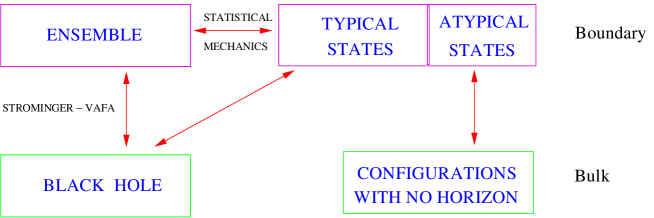
Figure 8: An schematic description of Possibility 1.

It is logically possible that, for the D1-D5-P system only, the path integrals in the bulk and on the boundary are related in the standard way via the $AdS$-CFT correspondence, and yet all the boundary states that give the CFT entropy are mapped into one black hole solution in the bulk. This possibility is depicted in Fig. 8. However, this possibility raises a lot of questions. First, why would the D1-D5-P system be different from all the other systems mentioned above. Moreover, from the microscopic (or CFT) perspective, there is nothing special about having three charges: One can map the boundary states in the D1-D5-KKM system in four dimensions to the corresponding bulk microstates [27, 96, 97]. The only reason for which the D1-D5-P system would be different from all the other systems would be the fact that it has the right amount of charges to create a macroscopically-large event horizon in five dimensions. To have such divergently different behaviour for the D1-D5-P system in five dimensions would be, depending on one’s taste, either very deep or, more probably, very bizarre.

Even if the typical states of the three-charge system correspond to one single black hole, we have seen that besides this black hole there exists a huge number of smooth solutions that also are dual to individual states of this CFT. Hence, according to Possibility 1, some states of the CFT would have individual bulk duals and some others would not (they would be dual as an ensemble to the black hole). This distinction is very unnatural. One might explain this if the states dual to the black hole and the ones dual to microstate geometries are in different sectors of the CFT, but this is simply not the case. We have seen in Section 8.6 that the deep bulk microstates correspond to boundary states that have one (or several) long component string(s). Hence, they belong to the same CFT sector as the typical microstates. If typical microstates did not have individual bulk duals, then in the same sector of the CFT we would have both states with a bulk dual and states without one. While not obviously wrong, this appears, at least, dubious and unjustifiable from the point of view of the CFT.

Possibility 2: Typical bulk microstate very similar to black hole.

It is possible that all the states of the CFT are dual to geometries in the bulk, but the typical states are dual to geometries that have a horizon, and that only differ from the classical black hole by some Planck-sized fuzz near the singularity. This situation is depicted in Fig. 9.

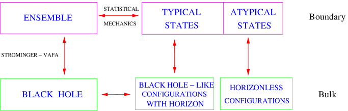
Figure 9: An schematic description of Possibility 2.

This also has a few problems. First, there are arguments, [12], that if the microstates of the black hole only differ from the classical geometry near the singularity, this does not solve the information paradox. Putting such arguments on one side, there is a more obvious objection: Possibility 2 means that typical microstates would have horizons, and so it would seem that one would have to ascribe an entropy to each microstate, which violates one of the principles of statistical mechanics. A counterargument here is to observe that one can always ascribe an ad hoc entropy to a microstate of any system simply by counting the number of states with the same macroscopic properties. What really distinguishes a microstate from an ensemble is that one has complete knowledge of the state of the former and that one has lost some knowledge of the state in the latter. The counterargument asserts that the presence of the horizon does not necessarily indicate information loss, and that the complete information might ultimately be extracted from something like the Hawking radiation. Thus microstates could have a horizon if information is somehow stored and not lost in the black hole. This is a tenable viewpoint and it is favored by a number of relativists but it defers the issue of how one decodes the microstate information to some unknown future physics whereas string theory appears to be pointing to a very interesting answer in the present.

There is also one of the objections raised in possibility 1: We have seen that some CFT states corresponding to long component strings are dual to deep microstates, that have no horizon. If the second possibility is correct, then other states in the same sector of the CFT would be dual to geometries that have a horizon and a singularity, and are therefore drastically different. Moreover, for extremal black holes, the distance to the horizon is infinite, while the distance to the cap of the microstates is finite (though divergent in the classical limit). Hence, in the same sector of the CFT, some states would be dual to supergravity solutions with an infinite throat, while others would be dual to solutions with a finite throat. This again appears quite dubious from the point of view of the CFT.

One can also think about obtaining the bulk microstate geometries by starting from a weak-coupling microstate (which is a certain configuration of strings and branes) and increasing the string coupling. During this process, we can imagine measuring the distance to the configuration. If a horizon forms, then this distance would jump from being finite to being infinite. However, for the smooth microstates, this distance is always a continuous function of the string coupling, and never becomes infinite. While the infinite jump of the length of the throat is a puzzling phenomenon, equally puzzling is the fact that only some microstates would have this feature, while some very similar ones would not.

Possibility 3: Typical bulk microstate differs from black hole at the scale of the horizon.

It is possible that all boundary microstates are dual to horizonless configurations. The classical black hole geometry is only a thermodynamic description of the physics, which stops being valid at the scale of the horizon, much like fluid mechanics stops being a good description of a gas at scales of order the mean free path. For physics at the horizon scale, one cannot rely on the thermodynamic description, and has to use a “statistical” description in terms of a large number of microstates. This possibility is depicted in Fig. 10.

Since these microstates have no horizon, they have unitary scattering but it takes a test particle a very long time to escape from this microstate. Hence, if this possibility is correct, the information paradox is reduced to nothing but an artifact of using a thermodynamic description beyond its regime of validity. This possibility now splits into two options, having to do with the appropriate description of the typical black hole microstates:

Possibility 3A: Typical microstates cannot be described in supergravity and require the full force of string theory.

Possibility 3B: Typical microstates can be described in supergravity.

As we cannot, yet, explore or count large strongly-interacting horizon-sized configurations of branes and strings using our current string theory technology, Possibility 3A would be more challenging to establish or analyze. We therefore need to examine Possibility 3B in great detail to see if it is true, or at least determine the extent to which supergravity can be used. One way to do this is by counting the microstates, using for example counting techniques of the type used in [13]. Another approach is to find the exact (or even approximate) dictionary between the states of the CFT and the bubbled geometries in the bulk. Anticipating (or perhaps speculating) a bit, one could imagine that, as a result of this investigation, one could relate the number of bubbles of a deep microstate to the distribution of the momentum on the long component string of the dual CFT state. Such a relation (which could in principle be obtained using scattering experiments as in [7, 23]) would indicate whether typical bulk microstates have large bubbles or Planck-sized bubbles, and would help distinguish between Possibilities 3A and 3B.

Figure 10: An schematic description of Possibility 3.

One of the interesting questions that needs to be addressed here is: What about non-extremal black holes?. All the arguments presented in this review in favor of the third possibility have been based on supersymmetric black holes, and one can legitimately argue that even if these black holes describe an ensemble of smooth horizonless configurations, it may be that non-supersymmetric black holes (like the ones we have in the real world) are fundamental objects, and not ensembles. The arguments put forth to support Possibility 3 for non-extremal black holes are rather more limited. Indeed, on a technical level, it is much more difficult to find non-supersymmetric, smooth microstate geometries, but some progress has been made [74]. There are nevertheless some interesting physical arguments based primarily on the phenomenon of charge fractionation.

The idea of charge fractionation [98, 99] is most simply illustrated by the fact that when you put $N_{1}$ D1 branes (or strings) in a periodic box of length $L$, then the lowest mass excitation carried by this system is not of order $L^{-1}$, but of order $(N_{1}L)^{-1}$. The explanation is that the branes develop multi-wound states with the longest effective length being of order $N_{1}L$. Similarly, but via a rather more complex mechanism, the lowest mass excitations of the D1-D5 system vary as $(N_{1}N_{5})^{-1}$. This is called charge fractionation. It is this phenomenon that leads to the CFT mass gap given in (273). The other important consequence of fractionation is that the corresponding “largest” natural physical length scale of the system grows as $N_{1}N_{5}$. One of the crucial physical questions is how does the “typical” length scale grow with charge. That is, what is the physical scale of the most likely (or typical) configuration. It is believed that this will grow as some positive power of the underlying charges, and this is the fundamental reason why it is expected that microstate geometries are “large” compared to the Planck scale and that microstate geometries are not just relevant within a few Planck units of the singularity, but extend to the location of the classical horizon.

This argument can be extended to non-BPS systems. Configurations of multiple species of branes also exhibit fractionation. For this reason, it is believed that, given a certain energy budget, the way to get most entropy is to make brane-antibrane pairs of different sorts. Putting together these different kinds of branes creates a system with very light (fractionated) modes, whose mass is much much lower than the Planck scale. These modes can then “extend” all the way to the horizon, and have to be taken into account when discussing physics at this scale.

One of the counterarguments to the third possibility is that one can collapse a shell of dust and create a horizon at very weak curvatures, long before the black hole singularity forms. Moreover, the larger the mass, the longer will be the time elapsed between the formation of the horizon and the singularity. Hence, it naively appears that the horizon cannot possibly be destroyed by effects coming from a singularity that is so far away. Nevertheless, if fractionation gives the correct physics, then one can argue that as the mass of the incoming shell increases, the number of brane-antibrane pairs that are created becomes larger, and hence the mass of the “fractionated” modes becomes smaller; these modes will then affect the physics at larger and larger scales, which can be argued to be of order the horizon size. In this picture the collapsing shell would reach a region where a whole new set of very light degrees of freedom exist. Since these “fractionated” degrees of freedom have a much larger entropy, the shell will dump all its energy into these modes, which would then expand to the horizon and destroy the classical geometry up to this scale. More details in support of these arguments can be found in [12].

On the other hand, one may hope to preserve the status quo for non-extremal black holes by arguing that fractionation is a phenomenon that is based on weakly coupled D-brane physics, and is not necessarily valid in the range of parameters where the black hole exists. This, however, leaves one with the problem of explaining why fractionation appears to be occurring in extremal black holes and why non-BPS black holes should be any different. Indeed, if the classical solution for the extremal black hole is proven to give an incorrect description of the physics at the horizon when embedded into a quantum theory of gravity, it is hard to believe that other similar, non-extremal solutions will give a correct description of the physics at the horizon. It will be much more reasonable to accept that all the classical black hole solutions are thermodynamic descriptions of the physics, which break down at the scale of the horizon.

The most direct support for the smooth microstate structure of non-extremal black holes would be the construction and counting of smooth, non-extremal geometries generalizing those presented here, like those constructed in [74]. Such constructions are notoriously difficult and, barring a technical miracle in the construction of non-BPS solutions, it is hard to hope that there will be a complete classification of such geometries in the near future. On the other hand, it is instructive and encouraging to recall the developments that happened shortly after the original state counting arguments of Strominger and Vafa for BPS black holes: There was a lot of analysis of near-BPS configurations and confirmation that the results could be generalized perturbatively to near-BPS states with small numbers of anti-branes. This might prove fruitful here and would certainly be very useful in showing that generic smooth microstate geometries are not special properties of BPS objects. It would thus be interesting to try, either perturbatively, or perhaps through microstate mergers, to create near-BPS geometries.

Finally, the fact that the classical black hole solution does not describe the physics at the scale of the horizon seems to contradict the expectation that this solution should be valid there since its curvature is very small. There are, however, circumstances in which this this expectation can prove wrong. First, if a solution has a singularity, it oftentimes does not give the correct physics even at very large distance away from this singularity because the boundary conditions at the singularity generate incorrect physics even in regions where the curvature is very low. Such solutions therefore have to be discarded. A few examples of such solutions are the Polchinski-Strassler flow [90] without brane polarization [91], or the singular KK giant graviton [93, 94]. The reason why we do not automatically discard black hole solutions is that their singularities are hidden behind horizons and sensible boundary conditions can be imposed at the horizon. However, this does not imply that all solutions with singularities behind horizons must be good: It only shows that they should not be discarded a priori, without further investigation. What we have tried to show is that if the third possibility is correct then the investigation indicates that the classical BPS black-hole solution should not be trusted to give a good description of the physics at the scale of the horizon.

9.2 A simple analogy

To understand Possibility 3 a little better, it is instructive to recall the physics of a gas, and to propose an analogy between the various descriptions of a black hole and the various descriptions of this gas.

For scales larger than the mean free path, a gas can be described by thermodynamics, or by fluid mechanics. At scales below the mean free path, the thermodynamic description breaks down, and one has to use a classical statistical description, in which one assumes all the molecules behave like small colliding balls. When the molecules are very close to each other, this classical statistical description breaks down, and we have to describe the states of this gas quantum mechanically. Moreover, when the temperature becomes too high, the internal degrees of freedom of the molecules become excited, and they cannot be treated as small balls. There are many features, such as shot noise or Brownian motion, that are not seen by the thermodynamic description, but can be read off from the classical statistical description. There are also features that can only be seen in the full quantum statistical description, such as Bose-Einstein condensation.

For black holes, if Possibilities 3A or 3B are correct, then the $AdS$-CFT correspondence relates quantum states to quantum states, and we expect the bulk dual of a given boundary state to be some complicated quantum superposition of horizonless configurations. Unfortunately, studying complicated superpositions of geometries is almost impossible, so one might be tempted to conclude that even if Possibilities 3A or 3B are correct, there is probably no new physics one can learn from it, except for an abstract paradigm for a solution to the information paradox. Nevertheless, we can argue by analogy to a gas of particles that this is not the case.

Consider a basis for the Hilbert space of the bulk configurations. If this basis is made of coherent states, some of the states in this basis will have a semiclassical description in terms of a supergravity background. This would be very similar to the situation explored in [86], where bubbled geometries correspond to coherent CFT states. The supergravity solutions we have discussed in these notes are examples of such coherent states. The main difference between the Possibility 3A and 3B has to do with whether the coherent states that form a basis of the Hilbert space can be described using supergravity or whether one has to use string theory to describe them. By analogy with the gas, this is the difference between the regime where the simple “colliding ball” model is valid, and the regime where one excites internal degrees of freedom of the molecules.

If supergravity is a good description of most of the coherent states, we can argue that we have constructed the black hole analogue of the classical statistical description of an ideal gas. Even if most of the coherent states can only be described in a full string-theoretic framework, one can still hope that this will give the analogue of an, albeit more complicated, classical statistical description of the gas. Both these descriptions are more complete than the thermodynamic description, and for the gas they capture physics that the thermodynamic description overlooks. Apart from solving the information problem, it would be very interesting to identify precisely what this physics is for a black hole. Indeed, as we will explain below, it might lead to some testable signature of string theory.

On the other hand, the black-hole analogue of the quantum statistical description involves a complicated and hard-to-study quantum superposition of microstates, and is therefore outside our present theoretical grasp. One can speculate, again in analogy with the ideal gas, that there are probably interesting physical phenomena that can only be captured by this description, and not by the classical statistical description.

We should also note that in [9] it has been argued that from the point of view of the dual CFT, the difference between the typical microstates and the classical black hole solution can only be discerned by doing a very atypical measurement, or waiting for a very long time. This is analogous to the case of a gas, where if one waits for a very long time, of order the Poincaré recurrence time, one will observe spikes in the pressure coming from very unlikely events, such as a very large number of molecules hitting the wall at the same time. In the thermodynamic approximation one ignores the small energy gap between microstates, and such phenomena are not visible. The fact that the classical black hole geometry has an infinite throat and no mass gap implies that this geometry will not display such fluctuations at very large time-scales. Since the CFT does have a mass gap, and fluctuations at large scales occur, one can argue [107] that the black hole gives a thermodynamic description of the physics, and not a microscopic one.

Since, by standard $AdS$-CFT arguments, a long time on the boundary corresponds to a large distance into the bulk, one can argue that atypical CFT measurements involving very long times correspond in the bulk to propagators that reach very close to the black hole horizon [9]. Hence, this supports the intuition that one can distinguish between different microstates by making experiments at the scale of the horizon. Moreover, in a gas one can distinguish between the ensemble and the microstates by making experiments at scales smaller than the mean free path. At this scale the thermodynamic description breaks down, and new phenomena that cannot be captured by thermodynamics appear. By analogy, for the black hole we have argued that the scale where thermodynamics breaks down is that of the horizon. Therefore, both our arguments and the arguments of [9] indicate that experiments made at the scale of the horizon should distinguish between a microstate and the classical solution. While from the point of the dual CFT these experiments appear to be very atypical, they might not be so atypical from the point of view of the dual bulk. It would certainly be very interesting to propose and analyze in more detail such gedanken experiments, and explore more thoroughly the implications of this fact.

The whole problem with finding experimental or observational tests of string theory is that the string scale and the Planck scale are so far out of reach of present accelerations. However, the ideas of fractionation and the present ideas about the microstate structure of black holes show us that we can get stringy effects on very large length scales. It would obviously be very exciting if we could make black holes at the LHC and thereby test these ideas, but even if this were not to happen, we may still be able to see some signature of stringy black holes within the next decade. Indeed, the gravitational wave detectors LIGO and LISA are very likely to detect the gravitational “ring-down” of merging black holes within the next few years and, while the underlying computations will be extremely difficult, one might reasonably hope that the microstate structure arising from string theory could lead to a new, detectable and recognizable signature in the LIGO or LISA data.

Acknowledgements

We would like to thank our collaborators, Per Kraus and Chih-Wei Wang, who played instrumental roles in much of the research reviewed here. We would also like to thank Samir Mathur, Gary Gibbons, Thibault Damour, Eric Gimon, Gary Horowitz, Don Marolf and Simon Ross, for interesting discussions that have helped us clarify many of the things presented here. IB would also like to thank Stefano Bellucci and Sergio Ferrara, for organizing the excellent Winter School on the Attractor Mechanism in Frascati, where the lectures on which these notes are based were given. NW and IB would like to thank CERN, the Institute for Advanced Study, and the Aspen Center for Physics where they were affiliated in the early stage of the writing of these notes. The work of NW was supported in part by funds provided by the DOE under grant DE-FG03-84ER-40168. The work of IB was supported in part by the NSF grant PHY-0503584, and by the Diréction des Sciences de la Matière of the Commissariat à L’Enérgie Atomique of France.

References

- [1] S. W. Hawking, “Breakdown Of Predictability In Gravitational Collapse,” Phys. Rev. D 14, 2460 (1976). “Particle Creation By Black Holes,” Commun. Math. Phys. 43, 199 (1975) [Erratum-ibid. 46, 206 (1976)].
- [2] A. Strominger and C. Vafa, “Microscopic Origin of the Bekenstein-Hawking Entropy,” Phys. Lett. B 379, 99 (1996) [arXiv:hep-th/9601029].
- [3] J. M. Maldacena, “The large N limit of superconformal field theories and supergravity,” Adv. Theor. Math. Phys. 2, 231 (1998) [Int. J. Theor. Phys. 38, 1113 (1999)] [arXiv:hep-th/9711200]. S. S. Gubser, I. R. Klebanov and A. M. Polyakov, “Gauge theory correlators from non-critical string theory,” Phys. Lett. B 428, 105 (1998) [arXiv:hep-th/9802109]. E. Witten, “Anti-de Sitter space and holography,” Adv. Theor. Math. Phys. 2, 253 (1998) [arXiv:hep-th/9802150].
- [4] M. Cvetic and A. A. Tseytlin, “Solitonic strings and BPS saturated dyonic black holes,” Phys. Rev. D 53, 5619 (1996) [arXiv:hep-th/9512031]. See also: M. Cvetic and D. Youm, “Dyonic BPS saturated black holes of heterotic string on a six torus,” Phys. Rev. D 53 (1996) 584 [arXiv:hep-th/9507090].
- [5] O. Lunin and S. D. Mathur, “AdS/CFT duality and the black hole information paradox,” Nucl. Phys. B 623, 342 (2002) [arXiv:hep-th/0109154].
- [6] O. Lunin and S. D. Mathur, “Statistical interpretation of Bekenstein entropy for systems with a stretched horizon,” Phys. Rev. Lett. 88, 211303 (2002) [arXiv:hep-th/0202072].
- [7] O. Lunin, J. M. Maldacena and L. Maoz, “Gravity solutions for the D1-D5 system with angular momentum,” arXiv:hep-th/0212210.
- [8] O. Lunin and S. D. Mathur, “The slowly rotating near extremal D1-D5 system as a ‘hot tube’,” Nucl. Phys. B 615, 285 (2001) [arXiv:hep-th/0107113]. L. F. Alday, J. de Boer and I. Messamah, “The gravitational description of coarse grained microstates,” arXiv:hep-th/0607222. A. Donos and A. Jevicki, “Dynamics of chiral primaries in AdS(3) x S**3 x T**4,” Phys. Rev. D 73, 085010 (2006) [arXiv:hep-th/0512017]. L. F. Alday, J. de Boer and I. Messamah, “What is the dual of a dipole?,” Nucl. Phys. B 746, 29 (2006) [arXiv:hep-th/0511246]. S. Giusto, S. D. Mathur and Y. K. Srivastava, “Dynamics of supertubes,” Nucl. Phys. B 754, 233 (2006) [arXiv:hep-th/0510235]. M. Taylor, “General 2 charge geometries,” JHEP 0603, 009 (2006) [arXiv:hep-th/0507223]. K. Skenderis and M. Taylor, “Fuzzball solutions and D1-D5 microstates,” arXiv:hep-th/0609154. N. Iizuka and M. Shigemori, “A note on D1-D5-J system and 5D small black ring,” JHEP 0508, 100 (2005) [arXiv:hep-th/0506215]. M. Boni and P. J. Silva, “Revisiting the D1/D5 system or bubbling in AdS(3),” JHEP 0510, 070 (2005) [arXiv:hep-th/0506085]. D. Martelli and J. F. Morales, “Bubbling AdS(3),” JHEP 0502, 048 (2005) [arXiv:hep-th/0412136]. Y. K. Srivastava, “Bound states of KK monopole and momentum,” arXiv:hep-th/0611124.
- [9] V. Balasubramanian, P. Kraus and M. Shigemori, “Massless black holes and black rings as effective geometries of the D1-D5 system,” Class. Quant. Grav. 22, 4803 (2005) [arXiv:hep-th/0508110].
- [10] I. Kanitscheider, K. Skenderis and M. Taylor, “Holographic anatomy of fuzzballs,” arXiv:hep-th/0611171.
- [11] A. A. Tseytlin, “Extreme dyonic black holes in string theory,” Mod. Phys. Lett. A 11, 689 (1996) [arXiv:hep-th/9601177]. A. A. Tseytlin, “Extremal black hole entropy from conformal string sigma model,” Nucl. Phys. B 477, 431 (1996) [arXiv:hep-th/9605091].
- [12] S. D. Mathur, “The fuzzball proposal for black holes: An elementary review,” Fortsch. Phys. 53, 793 (2005) [arXiv:hep-th/0502050]. S. D. Mathur, “The quantum structure of black holes,” Class. Quant. Grav. 23, R115 (2006) [arXiv:hep-th/0510180].
- [13] B. C. Palmer and D. Marolf, “Counting supertubes,” JHEP 0406, 028 (2004) [arXiv:hep-th/0403025]. V. S. Rychkov, “D1-D5 black hole microstate counting from supergravity,” JHEP 0601, 063 (2006) [arXiv:hep-th/0512053]. D. Bak, Y. Hyakutake and N. Ohta, “Phase moduli space of supertubes,” Nucl. Phys. B 696, 251 (2004) [arXiv:hep-th/0404104]. D. Bak, Y. Hyakutake, S. Kim and N. Ohta, “A geometric look on the microstates of supertubes,” Nucl. Phys. B 712, 115 (2005) [arXiv:hep-th/0407253].
- [14] D. Mateos and P. K. Townsend, “Supertubes,” Phys. Rev. Lett. 87, 011602 (2001) [arXiv:hep-th/0103030].
- [15] D. Mateos, S. Ng and P. K. Townsend, “Supercurves,” Phys. Lett. B 538, 366 (2002) [arXiv:hep-th/0204062].
- [16] R. Emparan, D. Mateos and P. K. Townsend, “Supergravity supertubes,” JHEP 0107, 011 (2001) [arXiv:hep-th/0106012].
- [17] O. Lunin and S. D. Mathur, “Metric of the multiply wound rotating string,” Nucl. Phys. B 610, 49 (2001) [arXiv:hep-th/0105136].
- [18] A. Sen, “Extremal black holes and elementary string states,” Mod. Phys. Lett. A 10, 2081 (1995) [arXiv:hep-th/9504147].
- [19] I. Bena and P. Kraus, “Three charge supertubes and black hole hair,” Phys. Rev. D 70, 046003 (2004) [arXiv:hep-th/0402144].
- [20] J. R. David, G. Mandal and S. R. Wadia, “Microscopic formulation of black holes in string theory,” Phys. Rept. 369, 549 (2002) [arXiv:hep-th/0203048].
- [21] O. Aharony, S. S. Gubser, J. M. Maldacena, H. Ooguri and Y. Oz, “Large N field theories, string theory and gravity,” Phys. Rept. 323, 183 (2000) [arXiv:hep-th/9905111].
- [22] S. Giusto, S. D. Mathur and A. Saxena, “Dual geometries for a set of 3-charge microstates,” Nucl. Phys. B 701, 357 (2004) [arXiv:hep-th/0405017].
- [23] S. Giusto, S. D. Mathur and A. Saxena, “3-charge geometries and their CFT duals,” Nucl. Phys. B 710, 425 (2005) [arXiv:hep-th/0406103].
- [24] S. Giusto and S. D. Mathur, “Geometry of D1-D5-P bound states,” Nucl. Phys. B 729, 203 (2005) [arXiv:hep-th/0409067].
- [25] S. Giusto, S. D. Mathur and Y. K. Srivastava, “A microstate for the 3-charge black ring,” arXiv:hep-th/0601193.
- [26] O. Lunin, “Adding momentum to D1-D5 system,” JHEP 0404, 054 (2004) [arXiv:hep-th/0404006].
- [27] I. Bena and P. Kraus, “Microstates of the D1-D5-KK system,” Phys. Rev. D 72, 025007 (2005) [arXiv:hep-th/0503053].
- [28] I. Bena and N. P. Warner, “Bubbling supertubes and foaming black holes,” Phys. Rev. D 74, 066001 (2006) [arXiv:hep-th/0505166].
- [29] P. Berglund, E. G. Gimon and T. S. Levi, “Supergravity microstates for BPS black holes and black rings,” JHEP 0606, 007 (2006) [arXiv:hep-th/0505167].
- [30] A. Saxena, G. Potvin, S. Giusto and A. W. Peet, “Smooth geometries with four charges in four dimensions,” JHEP 0604 (2006) 010 [arXiv:hep-th/0509214].
- [31] S. Giusto, S. D. Mathur and Y. K. Srivastava, “A microstate for the 3-charge black ring,” arXiv:hep-th/0601193.
- [32] I. Bena, C. W. Wang and N. P. Warner, “The foaming three-charge black hole,” arXiv:hep-th/0604110.
- [33] V. Balasubramanian, E. G. Gimon and T. S. Levi, “Four dimensional black hole microstates: From D-branes to spacetime foam,” arXiv:hep-th/0606118.
- [34] I. Bena, C. W. Wang and N. P. Warner, “Mergers and typical black hole microstates,” JHEP 0611, 042 (2006) [arXiv:hep-th/0608217].
- [35] M. C. N. Cheng, “More bubbling solutions,” arXiv:hep-th/0611156.
- [36] J. Ford, S. Giusto and A. Saxena, “A class of BPS time-dependent 3-charge microstates from spectral flow,” arXiv:hep-th/0612227.
- [37] I. Bena and P. Kraus, “Microscopic description of black rings in AdS/CFT,” JHEP 0412, 070 (2004) [arXiv:hep-th/0408186].
- [38] A. Dabholkar, “Exact counting of black hole microstates,” Phys. Rev. Lett. 94, 241301 (2005) [arXiv:hep-th/0409148].
- [39] S. Ferrara and R. Kallosh, “Supersymmetry and Attractors,” Phys. Rev. D 54, 1514 (1996) [arXiv:hep-th/9602136].
- [40] H. Ooguri, A. Strominger and C. Vafa, “Black hole attractors and the topological string,” Phys. Rev. D 70, 106007 (2004) [arXiv:hep-th/0405146].
- [41] P. Kraus, “Lectures on black holes and the AdS(3)/CFT(2) correspondence,” arXiv:hep-th/0609074. B. Pioline, “Lectures on on black holes, topological strings and quantum attractors,” Class. Quant. Grav. 23, S981 (2006) [arXiv:hep-th/0607227].
- [42] A. Sen, “How does a fundamental string stretch its horizon?,” JHEP 0505, 059 (2005) [arXiv:hep-th/0411255]. A. Dabholkar, F. Denef, G. W. Moore and B. Pioline, “Precision counting of small black holes,” JHEP 0510, 096 (2005) [arXiv:hep-th/0507014]. A. Dabholkar, F. Denef, G. W. Moore and B. Pioline, “Exact and asymptotic degeneracies of small black holes,” JHEP 0508, 021 (2005) [arXiv:hep-th/0502157]. A. Dabholkar, N. Iizuka, A. Iqubal, A. Sen and M. Shigemori, “Spinning strings as small black rings,” arXiv:hep-th/0611166. A. Dabholkar, A. Sen and S. Trivedi, “Black hole microstates and attractor without supersymmetry,” arXiv:hep-th/0611143.
- [43] D. Astefanesei, K. Goldstein and S. Mahapatra, “Moduli and (un)attractor black hole thermodynamics,” arXiv:hep-th/0611140. A. Sen, “Black hole entropy function and the attractor mechanism in higher derivative gravity,” JHEP 0509, 038 (2005) [arXiv:hep-th/0506177]. P. Kraus and F. Larsen, “Holographic gravitational anomalies,” JHEP 0601, 022 (2006) [arXiv:hep-th/0508218]. P. Kraus and F. Larsen, “Microscopic black hole entropy in theories with higher derivatives,” JHEP 0509, 034 (2005) [arXiv:hep-th/0506176]. S. Giusto and S. D. Mathur, “Fuzzball geometries and higher derivative corrections for extremal holes,” Nucl. Phys. B 738, 48 (2006) [arXiv:hep-th/0412133].
- [44] I. Bena and N. P. Warner, “One ring to rule them all … and in the darkness bind them?,” Adv. Theor. Math. Phys. 9 (2005) 667-701 [arXiv:hep-th/0408106.]
- [45] I. Bena, C. W. Wang and N. P. Warner, “Black rings with varying charge density,” JHEP 0603, 015 (2006) [arXiv:hep-th/0411072].
- [46] I. Bena, “Splitting hairs of the three charge black hole,” Phys. Rev. D 70, 105018 (2004) [arXiv:hep-th/0404073].
- [47] W. I. Taylor, “Adhering 0-branes to 6-branes and 8-branes,” Nucl. Phys. B 508, 122 (1997) [arXiv:hep-th/9705116].
- [48] J.D. Jackson, Classical Electrodynamics, Wiley, New York, NY, 1975.
- [49] J. C. Breckenridge, R. C. Myers, A. W. Peet and C. Vafa, “D-branes and spinning black holes,” Phys. Lett. B 391, 93 (1997) [arXiv:hep-th/9602065].
- [50] C. A. R. Herdeiro, “Special properties of five dimensional BPS rotating black holes,” Nucl. Phys. B 582, 363 (2000) [arXiv:hep-th/0003063].
- [51] G. T. Horowitz and J. Polchinski, “A correspondence principle for black holes and strings,” Phys. Rev. D 55, 6189 (1997) [arXiv:hep-th/9612146].
- [52] H. S. Reall, “Higher dimensional black holes and supersymmetry,” Phys. Rev. D 68, 024024 (2003) [arXiv:hep-th/0211290].
- [53] H. Elvang, R. Emparan, D. Mateos and H. S. Reall, “A supersymmetric black ring,” Phys. Rev. Lett. 93, 211302 (2004) [arXiv:hep-th/0407065].
- [54] H. Elvang, R. Emparan, D. Mateos and H. S. Reall, “Supersymmetric black rings and three-charge supertubes,” Phys. Rev. D 71, 024033 (2005) [arXiv:hep-th/0408120].
- [55] J. P. Gauntlett and J. B. Gutowski, “General concentric black rings,” Phys. Rev. D 71, 045002 (2005) [arXiv:hep-th/0408122].
- [56] S. W. Hawking, “Gravitational Instantons,” Phys. Lett. A 60, 81 (1977).
- [57] D. Gaiotto, A. Strominger and X. Yin, “New connections between 4D and 5D black holes,” JHEP 0602, 024 (2006) [arXiv:hep-th/0503217].
- [58] D. Gaiotto, A. Strominger and X. Yin, “5D black rings and 4D black holes,” JHEP 0602, 023 (2006) [arXiv:hep-th/0504126].
- [59] H. Elvang, R. Emparan, D. Mateos and H. S. Reall, “Supersymmetric 4D rotating black holes from 5D black rings,” JHEP 0508, 042 (2005) [arXiv:hep-th/0504125].
- [60] I. Bena, P. Kraus and N. P. Warner, “Black rings in Taub-NUT,” Phys. Rev. D 72, 084019 (2005) [arXiv:hep-th/0504142].
- [61] I. R. Klebanov and A. A. Tseytlin, “Gravity duals of supersymmetric SU(N) x SU(N+M) gauge theories,” Nucl. Phys. B 578, 123 (2000) [arXiv:hep-th/0002159].
- [62] I. R. Klebanov and M. J. Strassler, “Supergravity and a confining gauge theory: Duality cascades and SB-resolution of naked singularities,” JHEP 0008, 052 (2000) [arXiv:hep-th/0007191].
- [63] A. W. Peet, “TASI lectures on black holes in string theory,” arXiv:hep-th/0008241.
- [64] R. Emparan and H. S. Reall, “Black rings,” Class. Quant. Grav. 23, R169 (2006) [arXiv:hep-th/0608012].
- [65] H. Elvang and P. Figueras, “Black Saturn,” arXiv:hep-th/0701035. R. Emparan and H. S. Reall, “A rotating black ring in five dimensions,” Phys. Rev. Lett. 88, 101101 (2002) [arXiv:hep-th/0110260]. R. Emparan, “Rotating circular strings, and infinite non-uniqueness of black rings,” JHEP 0403, 064 (2004) [arXiv:hep-th/0402149]. H. Elvang and R. Emparan, “Black rings, supertubes, and a stringy resolution of black hole non-uniqueness,” JHEP 0311, 035 (2003) [arXiv:hep-th/0310008].
- [66] I. Bena, C. W. Wang and N. P. Warner, “Sliding rings and spinning holes,” JHEP 0605, 075 (2006) [arXiv:hep-th/0512157].
- [67] G. W. Gibbons and S. W. Hawking, “Gravitational Multi - Instantons,” Phys. Lett. B 78, 430 (1978).
- [68] G. W. Gibbons and P. J. Ruback, “The Hidden Symmetries of Multi-Center Metrics,” Commun. Math. Phys. 115, 267 (1988).
- [69] J. P. Gauntlett, J. B. Gutowski, C. M. Hull, S. Pakis and H. S. Reall, “All supersymmetric solutions of minimal supergravity in five dimensions,” Class. Quant. Grav. 20, 4587 (2003) [arXiv:hep-th/0209114].
- [70] R. Kallosh and B. Kol, “E(7) Symmetric Area of the Black Hole Horizon,” Phys. Rev. D 53, 5344 (1996) [arXiv:hep-th/9602014].
- [71] F. Denef, “Supergravity flows and D-brane stability,” JHEP 0008, 050 (2000) [arXiv:hep-th/0005049]. B. Bates and F. Denef, “Exact solutions for supersymmetric stationary black hole composites,” arXiv:hep-th/0304094. F. Denef, “Quantum quivers and Hall/hole halos,” JHEP 0210, 023 (2002) [arXiv:hep-th/0206072].
- [72] K. Behrndt, G. Lopes Cardoso and S. Mahapatra, “Exploring the relation between 4D and 5D BPS solutions,” Nucl. Phys. B 732, 200 (2006) [arXiv:hep-th/0506251].
- [73] S.W. Hawking and G.F.R. Ellis, The Large Scale Structure of Space-Time, Cambridge University Press, 1975.
- [74] V. Jejjala, O. Madden, S. F. Ross and G. Titchener, “Non-supersymmetric smooth geometries and D1-D5-P bound states,” Phys. Rev. D 71, 124030 (2005) [arXiv:hep-th/0504181].
- [75] V. Cardoso, O. J. C. Dias, J. L. Hovdebo and R. C. Myers, “Instability of non-supersymmetric smooth geometries,” Phys. Rev. D 73, 064031 (2006) [arXiv:hep-th/0512277].
- [76] J. P. Gauntlett and J. B. Gutowski, “Concentric black rings,” Phys. Rev. D 71, 025013 (2005) [arXiv:hep-th/0408010].
- [77] M. Cyrier, M. Guica, D. Mateos and A. Strominger, “Microscopic entropy of the black ring,” Phys. Rev. Lett. 94, 191601 (2005) [arXiv:hep-th/0411187].
- [78] J. M. Maldacena, A. Strominger and E. Witten, “Black hole entropy in M-theory,” JHEP 9712, 002 (1997) [arXiv:hep-th/9711053].
- [79] M. Bertolini and M. Trigiante, “Microscopic entropy of the most general four-dimensional BPS black hole,” JHEP 0010, 002 (2000) [arXiv:hep-th/0008201].
- [80] R. Dijkgraaf, J. M. Maldacena, G. W. Moore and E. P. Verlinde, “A black hole farey tail,” arXiv:hep-th/0005003. P. Kraus and F. Larsen, “Partition functions and elliptic genera from supergravity,” arXiv:hep-th/0607138. J. de Boer, M. C. N. Cheng, R. Dijkgraaf, J. Manschot and E. Verlinde, “A farey tail for attractor black holes,” JHEP 0611, 024 (2006) [arXiv:hep-th/0608059].
- [81] G. T. Horowitz and H. S. Reall, “How hairy can a black ring be?,” Class. Quant. Grav. 22, 1289 (2005) [arXiv:hep-th/0411268].
- [82] M. Guica, L. Huang, W. Li and A. Strominger, JHEP 0610, 036 (2006) [arXiv:hep-th/0505188].
- [83] I. Bena and P. Kraus, “R**2 corrections to black ring entropy,” arXiv:hep-th/0506015.
- [84] R. Gopakumar and C. Vafa, “On the gauge theory/geometry correspondence,” Adv. Theor. Math. Phys. 3, 1415 (1999) [arXiv:hep-th/9811131].
- [85] C. Vafa, “Superstrings and topological strings at large N,” J. Math. Phys. 42, 2798 (2001) [arXiv:hep-th/0008142].
- [86] H. Lin, O. Lunin and J. M. Maldacena, “Bubbling AdS space and 1/2 BPS geometries,” JHEP 0410, 025 (2004) [arXiv:hep-th/0409174].
- [87] F. Cachazo, K. A. Intriligator and C. Vafa, “A large N duality via a geometric transition,” Nucl. Phys. B 603, 3 (2001) [arXiv:hep-th/0103067].
- [88] M. Cvetic and F. Larsen, “Near horizon geometry of rotating black holes in five dimensions,” Nucl. Phys. B 531, 239 (1998) [arXiv:hep-th/9805097].
- [89] J. M. Maldacena and L. Susskind, “D-branes and Fat Black Holes,” Nucl. Phys. B 475, 679 (1996) [arXiv:hep-th/9604042].
- [90] J. Polchinski and M. J. Strassler, “The string dual of a confining four-dimensional gauge theory,” arXiv:hep-th/0003136.
- [91] L. Girardello, M. Petrini, M. Porrati and A. Zaffaroni, “The supergravity dual of N = 1 super Yang-Mills theory,” Nucl. Phys. B 569, 451 (2000) [arXiv:hep-th/9909047].
- [92] K. Pilch and N. P. Warner, “N = 1 supersymmetric renormalization group flows from IIB supergravity,” Adv. Theor. Math. Phys. 4, 627 (2002) [arXiv:hep-th/0006066].
- [93] J. McGreevy, L. Susskind and N. Toumbas, “Invasion of the giant gravitons from anti-de Sitter space,” JHEP 0006, 008 (2000) [arXiv:hep-th/0003075]. M. T. Grisaru, R. C. Myers and O. Tafjord, “SUSY and Goliath,” JHEP 0008 (2000) 040 [arXiv:hep-th/0008015]. S. R. Das, A. Jevicki and S. D. Mathur, “Giant gravitons, BPS bounds and noncommutativity,” Phys. Rev. D 63, 044001 (2001) [arXiv:hep-th/0008088]. A. Hashimoto, S. Hirano and N. Itzhaki, “Large branes in AdS and their field theory dual,” JHEP 0008, 051 (2000) [arXiv:hep-th/0008016].
- [94] I. Bena and D. J. Smith, “Towards the solution to the giant graviton puzzle,” Phys. Rev. D 71, 025005 (2005) [arXiv:hep-th/0401173].
- [95] I. Bena and C. Ciocarlie, “Exact N = 2 supergravity solutions with polarized branes,” Phys. Rev. D 70, 086005 (2004) [arXiv:hep-th/0212252]. I. Bena and R. Roiban, “N = 1* in 5 dimensions: Dijkgraaf-Vafa meets Polchinski-Strassler,” JHEP 0311, 001 (2003) [arXiv:hep-th/0308013].
- [96] Y. K. Srivastava, “Perturbations of supertube in KK monopole background,” arXiv:hep-th/0611320.
- [97] Ashish Saxena, General 3-charge geometries in 4 dimensions (to appear)
- [98] S. R. Das and S. D. Mathur, “Excitations of D-strings, Entropy and Duality,” Phys. Lett. B 375, 103 (1996) [arXiv:hep-th/9601152].
- [99] J. M. Maldacena and L. Susskind, “D-branes and Fat Black Holes,” Nucl. Phys. B 475, 679 (1996) [arXiv:hep-th/9604042].
- [100] C. G. . Callan and J. M. Maldacena, “D-brane Approach to Black Hole Quantum Mechanics,” Nucl. Phys. B 472, 591 (1996) [arXiv:hep-th/9602043]. J. M. Maldacena, “Statistical Entropy of Near Extremal Five-branes,” Nucl. Phys. B 477, 168 (1996) [arXiv:hep-th/9605016].
- [101] U. H. Danielsson, A. Guijosa and M. Kruczenski, “Brane-antibrane systems at finite temperature and the entropy of black branes,” JHEP 0109, 011 (2001) [arXiv:hep-th/0106201].
- [102] R. Emparan and G. T. Horowitz, “Microstates of a neutral black hole in M theory,” Phys. Rev. Lett. 97, 141601 (2006) [arXiv:hep-th/0607023].
- [103] B. D. Chowdhury and S. D. Mathur, “Fractional brane state in the early universe,” arXiv:hep-th/0611330.
- [104] R. Gregory and R. Laflamme, “Black strings and p-branes are unstable,” Phys. Rev. Lett. 70, 2837 (1993) [arXiv:hep-th/9301052]. For a review see: T. Harmark, V. Niarchos and N. A. Obers, “Instabilities of black strings and branes,” arXiv:hep-th/0701022.
- [105] B. D. Chowdhury, S. Giusto and S. D. Mathur, “A microscopic model for the black hole - black string phase transition,” arXiv:hep-th/0610069.
- [106] T. Harmark, K. R. Kristjansson, N. A. Obers and P. B. Ronne, “Three-charge black holes on a circle,” arXiv:hep-th/0606246.
- [107] J. M. Maldacena, “Eternal black holes in Anti-de-Sitter,” JHEP 0304, 021 (2003) [arXiv:hep-th/0106112].
- [108] V. Balasubramanian, B. Czech, V. Hubeny, K. Larjo, M. Rangamani and J. Simon, “Typicality versus thermality: An analytic distinction,” arXiv:hep-th/0701122. V. Balasubramanian, J. de Boer, V. Jejjala and J. Simon, “The library of Babel: On the origin of gravitational thermodynamics,” JHEP 0512, 006 (2005) [arXiv:hep-th/0508023].