Domain wall cosmology and multiple accelerations

$\textrm{Bum-Hoon Lee}^{{\dagger},{\ddagger}}$, $\textrm{Wonwoo Lee}^{{\dagger}}$, $\textrm{Siyoung Nam}^{{\dagger}}$, and $\textrm{Chanyong Park}^{{\dagger}}$

^† CQUeST, Sogang University, Seoul, Korea 121-742

^‡ Department of Physics, Sogang University, Seoul, Korea 121-742

We classify the cosmological behaviors of the domain wall under junctions between two spacetimes in terms of various parameters: cosmological constants of bulk spacetime, a tension of a domain wall, and mass parameters of the black hole-type metric. Especially, we consider the false-true vacuum type junctions and the domain wall connecting between an inner AdS space and an outer AdS Reissner-Nordstr${\rm\ddot{o}}$m black hole. We find that there exist a solution to the junction equations with an inflation at earlier times and an accelerating expansion at later times.

PACS numbers: 98.80.cq , 11.27.+d

1 Introduction

The recent cosmological observations of high red shift supernova[1] and the measurements of angular fluctuations of cosmic microwave background fluctuations [2] imply that our present universe expands with acceleration, instead of deceleration. Thus, a theory describing our universe must incorporate in it the accelerating era at present as well as the early inflationary era. It is very interesting to construct a model explaining these facts.

The setups of the so-called bubble dynamics have opened the possibilities to search the cosmology on the bubble using the Israel junction equation. However, the junction equations only describe the evolution of the vacuum bubble and can not tell us about how to generate bubble. The possible mechanisms of bubble formations were studied ini the case of the true vacuum bubble case[3, 4, 5] and the false vacuum bubble[6, 7, 8, 9]. In [10, 11], the dS-S junction, the wall connecting the false vacuum inside it and the true vacuum outside it, was researched. Similarly, junctions among spacetimes with different cosmological constant, or vacuum energy, were also handled. See dS-SdS[12], dS-SAdS[13], dS-RN AdS[14] and references therein. However, the main interest of them was the observations in the bulk sides.

Recently, Randall and Sundrum (RS) [15, 16] made an interesting proposal that we may live in a four dimensional domain wall (or brane) of the five dimensional AdS spacetime. In this model, the metric fluctuation around the domain wall admits a bound state and the background cosmological constant makes this bound state a zero-mode to be identified as a graviton. The tension of the wall is fine tuned so that the effective cosmological constant on the domain wall is zero and becomes stationary. If the tension of wall is not fine tuned, it was shown that the domain wall can move in the five dimensional background space, which causes the inflationary cosmology on the domain wall [17]. Kraus pointed out that this inflation can be interpreted as the motion of the domain wall in a stationary background[18]. When two pieces of AdS spaces are glued along the moving domain wall, the junction equation determines the motion of the domain wall in terms of the domain wall tension and the two bulk cosmological constants.

When considering the false vacuum bubble solution, since an observer living in the outside space feels the positive energy lump at center, the outside space can be considered as a black hole-type metric by Birkhoff’s theorem[19]. From now on, we set the outside metric as a black hole type which gives rise to the maximally symmetric space turning off the black quantities like mass, charge and angular momentum.

In section 2, we will shortly review the junction equation. In section 3, when the outside space is a Schwarzschild black hole type metric, we will fully classify the cosmology of the domain wall according to the parameters which gives the same the qualitative behavior of the domain wall cosmology investigated by many authors. In section 4, when considering the outside space as a RN black hole type we will show that there can exist a multi-inflation solution, that describe the early time inflation as well as the late time acceleration. This solution can describe inflation of the early universe and of the present universe at the same time with the FRW expansion in the middle period. Here, though we find only one special solution showing the multi-accelerating behavior, it is also very interesting to find a parameter region describing the real world comparing with many cosmological data. In section 5, we close this paper with some discussion.

2 Junction Equations in Einstein Frame

In this section we will briefly review the method of deriving Israel’s junction equations from the variational principle. The reader who is familiar with the junction equation may skip this section. Let $M$ be a (D+1) dimensional manifold which a domain wall $\Sigma$ partitions into two parts $M_{\pm}$. We shall denote the two sides of $\Sigma$ as $\Sigma_{\pm}$, which are boundaries of both bulk $M_{\pm}$. We assume that each metric in the bulk $M_{\pm}$ is well defined solution of Einstein’s equation in the sense that we seek the whole solution of Einstein equation in the manifold $M$ as a distribute type. We also demand that the first junction condition should be satisfied so that across $\Sigma$ the tangential components of the metric $g_{\mu\nu}^{\pm}$ are continuous, which states that the induced metrics from both sides $M_{\pm},$ must be the same. The condition originates from the fact that the derivative of a step function is a delta function which generates a singular term in the connection. The second junction condition deals about the derivative of the metrics $g_{\mu\nu}^{\pm}$. For a later convenience, we now introduce such a useful notation that

$$[A]\equiv A^{+}|_{\Sigma_{+}}-A^{-}|_{\Sigma_{-}}$$ (1)

where each $A^{\pm}$ is a tensorial quantities defined in $M_{\pm}$. The second junction condition can be written as

$$[K_{ij}]=0$$ (2)

where $K_{ij}$ is a extrinsic curvature which will be defined below. In a coordinate system it is simply proportional to the derivative of the metric. The second junction condition plays a role of removing the $\delta$-function terms from the Einstein equations and is a sufficient condition for the regular behavior of the full Riemann tensor at the hypersurface $\Sigma$. If this condition is violated, then it means that the spacetime is singular at $\Sigma$. We can cure this problem by the following method. If the extrinsic curvature is not the same on both sides of $\Sigma$, then a thin shell with the $\delta$ function-like stress-energy tensor must be present at $\Sigma$, which the junction equations tell us about. This situation is similar to the eletrostaic problem where a surface layer of nonzero electric charge density exists between two different mediums. This sheet generates a discontinuity in the electric field and a kink in the electrostatic potential, which is completely analogous to the gravitational case. These physical meanings can be embodied more definitely in deriving the junction equations, which starts from an action

$$S_{total}=S_{EH}+S_{GH}+S_{DW}$$ (3)

where

$$S_{EH} = \frac{1}{2\kappa^{2}}\int_{M}d^{D+1}x\sqrt{-g}~{}(R-2\Lambda),$$ (4)

$$S_{GH} = \frac{1}{\kappa^{2}}\int_{\Sigma_{\pm}}d^{D}x\sqrt{-h}K,$$ (5)

$$S_{DW} = \int_{\Sigma}d^{D}x\sqrt{-h}{\cal L}_{DW}.$$ (6)

We set $\kappa^{2}=8\pi G$ and $\Lambda$ cosmological constants. $n^{\rho}$ is a unit normal vector and $h_{\mu\nu}=g_{\mu\nu}-n_{\mu}n_{\nu}$ is the metric induced on $\Sigma_{\pm}$. $K=h^{ij}K_{ij}$ is the trace of the extrinsic curvature $K_{ij}=h^{\phantom{k}k}_{i}h^{\phantom{k}l}_{j}\nabla_{k}n_{l}$ on $\Sigma_{\pm}$. $S_{EH}$ is the ordinary Einstein-Hilbert action. For a good variational problem we must include the Gibbons-Hawking action $S_{GH}$[20]. Varying $S_{EH}$ with respect to each bulk metric generates boundary terms which contain normal derivatives of the metric variations and their presence will spoil the variational principle leading to Einstein’s equations. The terms from the metric variations of $S_{GH}$ exactly cancel the boundary terms of the normal derivatives of the metric in $S_{EH}$[21]. Due to discontinuities of $K_{\mu\nu}$ across $\Sigma$, the contributions from $\Sigma_{\pm}$ need not cancel each other. Thus we need a domain wall action. In general, when the gravitational back-reaction of a domain wall is included, the global causal structure of the resulting spacetime is usually modified. For simplicity, we assume that no bulk fields do not couple to the domain wall, whose world volume can be described as a Nambu-Goto action

$$S_{DW}=-\sigma\int_{\Sigma}d^{D}x\sqrt{-h}$$ (7)

where $\sigma$ is a parameter which corresponds to a tension or energy density of the wall $\Sigma$. There can be no transfer of energy between the bulk matter and the wall because the energy density of the wall is fixed. In this case, the stress-energy tensor of the domain wall is proportional to the wall’s induced metric tensor $h_{ij}$. Now the metric variations of the total action $S_{total}$ give the Israel’s junction equations

$$[K_{ij}]=\kappa^{2}\left(S_{ij}-\frac{1}{D-1}Sh_{ij}\right)$$ (8)

where a stress tensor of the wall, tangential to the domain wall, is defined by

$$S_{ij}\equiv\frac{2}{\sqrt{-h}}\frac{\delta S_{DW}}{\delta h^{ij}}.$$ (9)

With $S_{ij}=\sigma h_{ij}$, then the junction equations take a simple form

$$[K_{ij}]=-\chi_{D}h_{ij}$$ (10)

where

$$\chi_{D}=\frac{8\pi G_{D+1}\sigma}{D-1}.$$ (11)

For applications of the junctions equations, we assume that each bulk has a spherical symmetry such that the bulk metric has the form

$$ds^{2}=-H(R)dT^{2}+\frac{dR^{2}}{H(R)}+R^{2}d\Omega^{2}_{D-1}$$ (12)

where

$$H(R) \equiv 1-AR^{2}-\frac{Bw_{D}G_{D+1}M}{R^{D-2}},$$ (13)

$$w_{D} \equiv \frac{16\pi}{(D-1)V_{D-1}},$$ (14)

$$V_{D-1} \equiv \frac{2\pi^{D/2}}{\Gamma(D/2)},$$ (15)

and $M$ is a black hole mass if any. The parameters represent the followings : If a bulk resembles a black hole-like one, $B=1$. Otherwise, $B$ is zero. The constant $A$ is related with a cosmological constant, so that $A=e/L^{2}=2e\Lambda/D(D-1)$ with $e=+1$ for dS space and $e=-1$ for AdS space. We choose a positive direction so that makes the radial coordinate with fixed angular components increase. Due to the spherical symmetry, the induced metric on the wall can be rewritten as

$$ds^{2}_{wall}=-d\tau^{2}+r(\tau)^{2}d\Omega^{2}_{D-1}$$ (16)

where $\tau$ is the proper time of the world line of the observer on the wall and satisfy the relation

$$d\tau^{2}=H(r)dt^{2}-\frac{1}{H(r)}dr^{2}$$ (17)

with our convention that the bulk coordinates on the position corresponding to the domain wall use lowercase letters. We will interpret the radial coordinate of the domain wall as a scale factor $r(\tau)$ from the viewpoint of the wall observer’s. At this point, we introduce the Gauss normal coordinates near the wall $\Sigma$, which require

$$g^{\eta\eta}=g_{\eta\eta}=1.$$ (18)

In these coordinates, the extrinsic curvatures take very simple forms

$$K^{\theta}_{\phantom{\mu}\theta} = K^{\phi}_{\phantom{\mu}\phi}=\cdots=\frac{\epsilon\sqrt{\dot{r}^{2}+H(r)}}{r}$$ (19)

$$K^{\tau}_{\phantom{\mu}\tau} = \frac{\epsilon}{\sqrt{\dot{r}^{2}+H(r)}}\left(\ddot{r}+\frac{1}{2}\frac{dH(r)}{dr}\right)$$ (20)

at the location of the wall $R=R(r(\tau))$. If the spherical surface area increases with the radial coordinate, $\epsilon=+1$ and $\epsilon=-1$ otherwise. The dot represents a derivative with respect to the proper time $\tau$ of an observer’s worldline on the wall. Note that the angular parts of the extrinsic curvature are diagonalized and have the same value at each point of the wall due to the spherical symmetry. Plugging (19) into (10) results in the equation

$$\epsilon_{out}\sqrt{\dot{r}^{2}+H_{out}(r)}-\epsilon_{in}\sqrt{\dot{r}^{2}+H_{in}(r)}=-\chi_{D}r,$$ (21)

or

$${\dot{r}}^{2}-\frac{(H_{out}-H_{in})^{2}}{4\chi_{D}^{2}r^{2}}-\frac{1}{4}\chi_{D}^{2}r^{2}+\frac{1}{2}(H_{out}+H_{in})=0$$ (22)

where the subscripts $out$(or $+$) and $in$(or $-$) represent the outer side and the inner side of the wall respectively. After a short algebra with the explicit forms of $H_{\pm}$, the above equation can finally be rewritten as

$$\frac{1}{2}{\dot{r}}^{2}+V(r)=-\frac{1}{2}$$ (23)

where the effective potential is

$$V(r) = -\frac{r^{2}}{8}\left[\frac{(A_{out}-A_{in})^{2}}{\chi_{D}^{2}}+\chi_{D}^{2}+2(A_{out}+A_{in})\right]$$ (24)

$$-\frac{G_{D+1}w_{D}}{4r^{D-2}}\left[\frac{(A_{out}-A_{in})(B_{out}M_{out}-B_{in}M_{in})}{\chi_{D}^{2}}+(B_{out}M_{out}+B_{in}M_{in})\right]$$

$$-\frac{G_{D+1}^{2}w^{2}_{D}(B_{out}M_{out}-B_{in}M_{in})^{2}}{8\chi_{D}^{2}r^{2D-2}}.$$

This equation of motion describes a fictitious particle moving under the effective potential $V(r)$ with the energy $-\frac{1}{2}$ analogous to a 1-dimensional classical particle of energy E influenced by the potential $V$, which we know how to deal very well. The remaining thing is classifying the allowed solutions of the wall under the given effective potential. The strategy is as follows. At first, we start to find out the possible shapes of the potential by collecting information about the extreme values of the potential. The second, we simply compare the extreme values of the potential with the energy $-1/2$. If the maximum of the potential is always lower than $-1/2$, then we call the motion of the wall as a ‘monotonic’ motion because it expands monotonically without bounds. If there is a region in which the potential is higher than the energy of the wall, the wall’s motion will also be restricted. In this case, if the wall has a maximum(minimum) radius to which it expands, we call the corresponding solution as a ‘bounded’(‘bounce’) solution whose meaning is clear.

3 Classifications of the wall motions

Now, consider the junction equation describing the connection between a maximally symmetric spacetime at center and a black hole type spacetime in the outside region. In general, the junction equation is given by

$$\epsilon_{in}\sqrt{\dot{r}^{2}+H_{in}}-\epsilon_{out}\sqrt{\dot{r}^{2}+H_{out}}=\chi_{D}r$$ (25)

with

$$H_{in} = -A_{in}r^{2}+1$$

$$H_{out} = -A_{out}r^{2}+1-\frac{Bw_{D}G_{D+1}M}{r^{D-2}}.$$ (26)

Though the solution of the junction equation is obtained from solving (24), we can find some constraints for the region of $r$ from (25). Since the tension $\sigma$ is positive and $r$ runs form $0$ to $\infty$, depending on the sign of $\epsilon$ the region of $r$ having a solution is restricted:
1) $\epsilon_{in}=\epsilon_{out}=1$
Having a solution, the position of the wall is located at the restricted region $r^{D}<\frac{Bw_{D}G_{D+1}M}{A_{in}-A_{out}+\chi_{D}^{2}}$, where we set $A_{in}-A_{out}$ to a positive number.
2) $\epsilon_{in}=\epsilon_{out}=-1$
In this case, the region of the wall position is restricted as $r^{D}>\frac{Bw_{D}G_{D+1}M}{A_{in}-A_{out}-\chi_{D}^{2}}$.
3) $\epsilon_{in}=-\epsilon_{out}=1$
The wall is located at the region $\frac{Bw_{D}G_{D+1}M}{A_{in}-A_{out}+\chi_{D}^{2}}<r^{D}<\frac{Bw_{D}G_{D+1}M}{A_{in}-A_{out}-\chi_{D}^{2}}$ in $r$-direction.
4) $-\epsilon_{in}=\epsilon_{out}=1$
In this case, there is no region having a solution.

When solving (24), the above restricted region corresponding to each case is also considered.

3.1 (D+1)-dimensional M-SAdS Junction

In this section we consider the M-SAdS type junction which is described by the parameters

$$A_{out}=-\frac{2\Lambda_{out}}{D(D-1)}~{},~{}B_{out}=1~{},~{}M_{out}=M~{},~{}\textrm{and~{} the~{} others~{} zero}.$$ (27)

A positively-defined quantity $\chi_{+}$ is related to the vacuum energy of the outer SAdS space. For convenience, we introduce the ratios among the parameters by

$$u\equiv\frac{1}{\chi_{D}}\sqrt{\frac{2\Lambda_{out}}{D(D-1)}}~{}~{}\textrm{and}~{}~{}v\equiv\frac{m}{(D-1)\chi_{D}}$$ (28)

where

$$m=(D-1)w_{D}G_{D+1}M$$ (29)

roughly corresponds to the mass density proportional to the black hole mass divided by the volume of the unit sphere $S^{D-1}$. The effective potential (24) becomes to

$$V(r) = -\frac{1}{8}(u^{2}-1)^{2}\chi_{D}^{2}r^{2}+\frac{v(u^{2}-1)\chi_{D}}{4r^{D-2}}-\frac{v^{2}}{8r^{2D-2}}$$ (30)

$$= -\frac{1}{8}\left((u^{2}-1)\chi_{D}r-\frac{v}{r^{D-1}}\right)^{2}$$

Therefore, the scheme of classifying the possible wall motion of $M-SAdS$ junction can depend on the signs of $u$ and $v$.

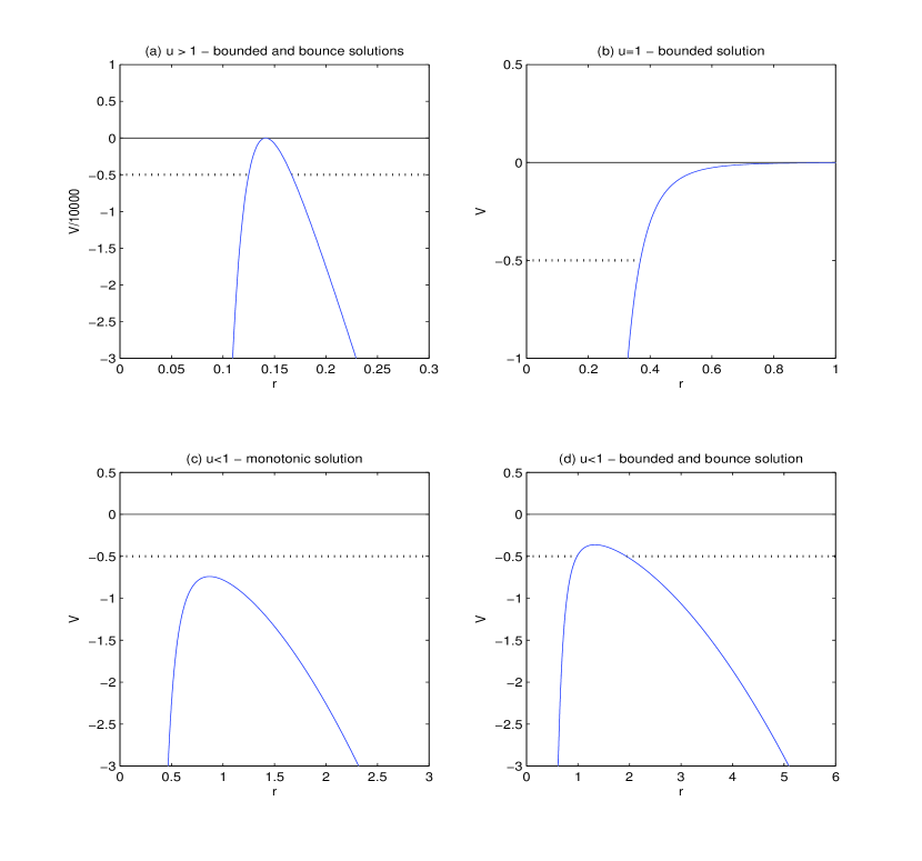
Figure 1: Classification of the possible motions of the wall in the 5 dimensional M-SAdS junction. We set $w_{4}G_{5}M=1$ in all case for simplicity. (a) $u=50$ and $\chi_{4}=1$ (b) $u=1$ and $\chi_{4}=10$ (c) $u=0.2$ and $\chi_{4}=1$ (d) $u=0.4$ and $\chi_{4}=2.5$.

3.1.1 $u>1$

The value of the effective potential asymptotically diverges to $-\infty$ as the radial coordinate goes to zero or infinity. This means that there exists one critical point at which the potential has a maximum value. The point is given by

$$r^{D}_{c}=\frac{v}{\chi_{D}(u^{2}-1)},$$ (31)

at which the potential really has a maximum value equal to zero. Therefore, the motions of the wall are limited to the bounded one or the bounce one(Fig. 1(a)). In the bounce solution, the late time behavior of the solution(large $r$) is

$$r\approx e^{\frac{\chi_{D}(u^{2}-1)}{2}\tau}$$ (32)

independent of $m$.

3.1.2 $u=1$

The effective potential is

$$V(r)=-\frac{v^{2}}{8r^{2D-2}}.$$ (33)

The only allowed solution of the junction equation is a bounded type(Fig.1(b)), which can expand to a maximum radius

$$r_{max}=\left(\frac{v}{2}\right)^{\frac{1}{D-1}}$$ (34)

and then shrink. In terms of $r_{max}$, the potential can be rewritten by

$$V=-\frac{1}{2}\left(\frac{r_{max}}{r}\right)^{2D-2}$$ (35)

and the trajectory $r=r(\tau)$ of the wall can be found by integrating

$$\pm\tau=\int_{r(0)}^{r(\tau)}\frac{dr^{\prime}}{\sqrt{\left(\frac{r_{max}}{r^{\prime}}\right)^{2(D-1)}-1}}$$ (36)

and getting the inverse of it. Around the origin the behavior of the radius of the wall is

$$r\approx\left(Dr_{max}^{D-1}\cdot\tau\right)^{\frac{1}{D}}.$$ (37)

3.1.3 $u<1$

The effective potential of this case resembles the shape of the $u>1$ case. A extreme point of the potential occurs at

$$r^{D}_{c}=\frac{(D-1)v}{\chi_{D}(1-u^{2})}.$$ (38)

$V(r_{c})$ corresponds to the maximum of the curve of the effective potential and is always negative. Therefore, the possible solutions can be classified by comparing $V(r_{c})$ and the energy of the virtual one-particle. If $V(r_{c})<-1/2$, then a monotonic motion is possible(Fig. 1(c)). If $V(r_{c})>-1/2$ , then a bounced or bounded motion is allowed(Fig. 1(d)).

3.1.4 Summary of the M-SAdS Junction

We can classify the wall motions under the M-SAdS junctions by $u$, $v$ and $\chi_{D}$. The extreme points $r_{c}$ are the solutions of the ordinary second equation with respect to the variable $r_{c}^{D}$. The classification corresponds to the regions separated by surfaces in the 3-dimensional parameter space $(\chi_{D},u,v)$. For $u>1$, the allowed solutions are bounded or bounce ones. For $u=1$, the possible solution is limited to a bounded type. For $u<1$, we need further information about $v$ and $\chi_{D}$ to classify the wall motions completely in this parameters’ ranges. We found that all the 3-type motions are allowed in that case.

3.2 (D+1)-Dimensional AdS-SAdS Junctions

We set

$$H_{out} = 1+\frac{2\Lambda_{out}}{D(D-1)}R^{2}-\frac{w_{D}G_{D+1}M}{R^{D-2}},$$ (39)

$$H_{in} = 1+\frac{2\Lambda_{in}}{D(D-1)}R^{2}.$$ (40)

For simplicity, we introduce another parameter ratio

$$w\equiv\frac{1}{\chi_{D}}\sqrt{\frac{2\Lambda_{in}}{D(D-1)}}.$$ (41)

According to (24), the effective potential is given by

$$V(r)=-\frac{1}{8}\alpha\chi_{D}^{2}r^{2}+\frac{\beta\chi_{D}v}{4r^{D-2}}-\frac{v^{2}}{8r^{2D-2}}$$ (42)

where

$$\alpha=\beta^{2}-4w^{2}~{}~{}\textrm{and}~{}~{}\beta=u^{2}-w^{2}-1.$$ (43)

Thus, the classification corresponds to divide the 4-dimensional parameter space $(\chi_{D},u,v,w)$ into regions by the judicious surfaces of the parameters. The regions described by the curves $u>w$ in the $u-w$ plane represent the junctions of the true-false vacuum type. Since we want to concentrate on the false-true vacuum types, the regions with positive $\beta$ are discarded. To see this, note that $u=\pm w$ are asymptotes of the hyperbola $\beta=0$ in $u-w$ plane. In this section, we have always the condition $0<u<w$ in mind. We also set every parameters to be positive. Of course, we could deal with the cases allowing the negative ranges of the parameters but that simply results in the mirror image with respect to the appropriate axes or curves in the $u-w$ plane. In this paper, we ignore the possibilities of those regions and the physical meanings of the negative range of the parameters.

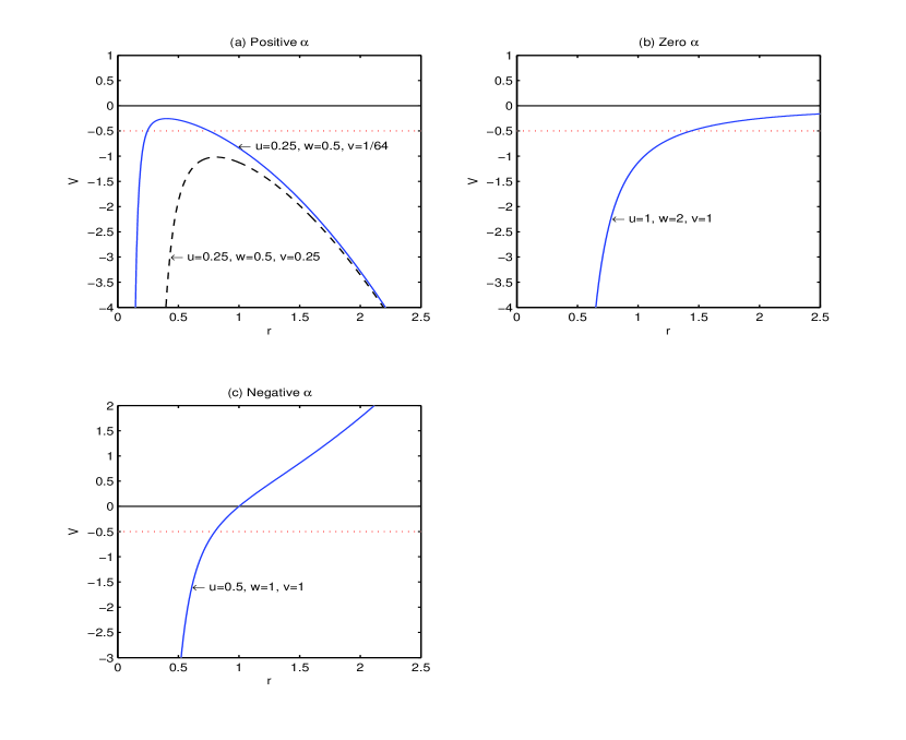
Figure 2: Classifying the possible motions of the wall in the AdS-SAdS junction by $\alpha$

3.2.1 $\alpha>0$

The condition $\alpha>0$ is translated into $\beta<-2w$(Fig. 2(a)). There are two regions in $u-w$ plane. The first region is surrounded by

$$0<u<w~{}~{}\textrm{and}~{}~{}u+w-1<0$$ (44)

and the second is enclosed by the curves

$$0<u<w~{}~{}\textrm{and}~{}~{}u-w+1<0.$$ (45)

From the analysis of the asymptotic behaviors of the effective potential, it is expected that the potential have only one extreme point $r_{c}$. By an explicit calculation, we find that it really does so that the extreme point is

$$r_{c}^{D}=\frac{v}{2\alpha\chi_{D}}\left[-(D-2)\beta+\sqrt{(D-2)^{2}\beta^{2}+4(D-1)\alpha}\right],$$ (46)

at which the potential has a maximum. The solutions in the ranges of these parameters can be classified by comparing the value of the maximum of the potential $V(r_{c})$ and the energy. If $V(r_{c})$ is greater than the energy, the motion of the wall can be either bounded or bounced type. Otherwise, the possible motion of it should be a monotonic one.

3.2.2 $\alpha=0$

The condition $\alpha=0$(Fig. 2(b)) corresponds to a straight line

$$u=\mid w-1\mid$$ (47)

for $1/2<w$ except a point $(u,w)=(0,1)$. Therefore, two different modes may exist. One corresponds to $w-u=1$ and the other corresponds to $w+u=1$. From the analysis of the potential, it is easy to see that there is only a bounded motion of the wall.

3.2.3 $\alpha<0$

The negative $\alpha$ means that $\beta$ is in the range

$$-2w<\beta<0,$$ (48)

which corresponds to a strip in the $u-w$ plane surrounded by

$$0<u<w~{}~{}\textrm{and}~{}~{}u=\mid w-1\mid$$ (49)

for $1/2<w$ except a point $(u,w)=(0,1)$(Fig. 2(c)). The effective potential can be rewritten as

$$V(r)=\frac{1}{8}\mid\alpha\mid\chi_{D}^{2}r^{2}+\frac{\beta\chi_{D}v}{4r^{D-2}}-\frac{v^{2}}{8r^{2D-2}},$$ (50)

which is expected to have two positive real critical points of the potential or no such ones to explain the asymptotic behaviors of the potential naturally. Since the expressions for two extremal points are given by

$$r_{c\pm}^{D}=\frac{v}{2\mid\alpha\mid\chi_{D}}\left[(D-2)\beta\pm\sqrt{D^{2}\beta^{2}-16(D-1)w^{2}}\right],$$ (51)

with a negative $\beta$, the potential can not have two extreme points. We conclude that the motion of the wall is always bounded in the range of negative $\alpha$.

3.2.4 Summary of the AdS-SAdS Junctions

The possible types of the motion of the wall is more complicated than the ones of the previous section since we turned on the negative cosmological constant inside the wall and set the outer metric to be the form of the Schwarzschild AdS type. We can classify the motions of the wall simply as dividing the first quadrant in the $u-w$ plane into several regions according to the sign of $\alpha$ and $\beta$. The monotonic type solution can only exist in the case of $\alpha<0$.

3.3 Classifying Scheme to the other (D+1)-dimensional Junctions

In this section, we will apply our classifying scheme to the other spherical false-true vacuum type of junctions. The dS-S, dS-SdS, dS-AdS cases have been handled in many other papers about the bubble dynamics and their possible wall motions are a bounded or bounce or monotonic type again. But their classifications dependent on the parameters used are not given completely. As an exercise for applying our scheme, we consider and try to classify them again.

3.3.1 (D+1)-dimensional dS-SdS Junctions

To classify solutions of a junction, we must know what effective potential it has. There are two ways that we can do this. The one is that we simply assume the forms of the bulk metrics as in the equation (12) and use the formula (24) and the other is that we change the signs of the combinatory parameters $u^{2}$ and $w^{2}$ appropriately. We follow the latter way in this subsections. Given the effective potential, we can classify the wall motions from a wall observer’s view. The coefficients of the bulk metrics in the dS-SdS junction are

$$A_{in}=w^{2}\chi_{D}^{2}~{},~{}A_{out}=u^{2}\chi_{D}^{2}~{},~{}M_{out}=M~{}\textrm{and ~{}the~{} others ~{}zero}.$$ (52)

Because one of the differences between the dS space and the AdS space is that they differ each other in the vacuum energies, we flip the signs of $u^{2}$ and $w^{2}$ and substitute them in the AdS-SAdS case. Thus the effective potential is given by

$$V(r)=-\frac{1}{8}\alpha\chi_{D}^{2}r^{2}-\frac{\beta\chi_{D}v}{4r^{D-2}}-\frac{v^{2}}{8r^{2D-2}}$$ (53)

where

$$\alpha=\beta^{2}+4w^{2}~{}~{}\textrm{and}~{}~{}\beta=u^{2}-w^{2}+1.$$ (54)

Since the effective potential is given, we can classify the solutions by the signs of $\alpha$ and $\beta$ and the expected forms of the potential. We omit the detailed analysis of this junction.

3.3.2 (D+1)-dimensional dS-AdS Junctions

In this case, we can get the effective potential by $u^{2}\rightarrow-u^{2}$ and $v=0$ in the potential of the dS-SdS junction (53) or by $w^{2}\rightarrow-w^{2}$ and $v=0$ in the potential of the AdS-SAdS junction (42). The result is

$$V(r)=-\frac{1}{8}\alpha\chi_{D}^{2}r^{2}-\frac{\beta\chi_{D}v}{4r^{D-2}}$$ (55)

where

$$\alpha=\beta^{2}+4w^{2}~{}~{}\textrm{and}~{}~{}\beta=u^{2}+w^{2}+1.$$ (56)

3.3.3 (D+1)-dimensional dS-S Junctions

This case simply corresponds to the $dS-SdS$ junctions with replacing $u$ by zero, that is, we turn off $\Lambda_{out}$. Thus the effective potential is

$$V(r)=-\frac{1}{8}(1+w^{2})^{2}\chi_{D}^{2}r^{2}-\frac{\chi_{D}v(1+w^{2})}{4r^{D-2}}-\frac{v^{2}}{8r^{2D-2}}.$$ (57)

4 AdS - RN AdS Junctions

In this section we will deal with the junction equation which connects the inner AdS space to the outer Reissner-Nordstr$\ddot{o}$m AdS space. To describe the Reissner-Nordstr$\ddot{o}$m AdS space, we consider the charged particles spread uniformly on the domain wall. In string theory set-up, the domain wall in the asymptotically AdS space corresponds to the D3-brane and the charged particles correspond not to the fluctuations of open string on D3-brane but to D5-branes wrapped on $S^{5}$ in $AdS_{5}\times S^{5}$. After some compatification mechanism, these D5-branes look like charged particles in $AdS_{5}$ space and become the sources of the bulk 1-form gauge field. So the action describing this situation is

$$S = \frac{1}{2\kappa^{2}}\int_{M}d^{D+1}x\sqrt{-g}\left(R-2\Lambda\right)-\frac{1}{4}\int_{M}d^{D+1}x\sqrt{-g}F^{2}+\frac{1}{\kappa^{2}}\int_{\Sigma_{\pm}}d^{D}x\sqrt{-h}K$$ (58)

$$-\int_{\Sigma}d^{D}x\sqrt{-h}\sigma+\int_{\Sigma}d^{D}x\sqrt{-h}qC_{0}$$

with

$$F_{r0}=\partial_{r}C_{0},$$ (59)

where $q$ is a constant charge density on the domain wall and the total charge $Q$ is given by $Q=\int_{\Omega_{3}}d^{3}x\sqrt{h^{\prime}}q$ with the three sphere metric, $h^{\prime}$. Note that the tension $\sigma$ is the sum of that of D3-brane and the energy density of charged particles. In the inner region of the wall where there is no source, the solution of the equation of motion for the gauge field is given by $F=0$. Using this result, we can easily find that in the inner region the pure AdS space becomes the solution of the Einstein equation. In the outside region, the charged particles gives the non-zero gauge field. In the asymptotic region, due to the cosmological constant the metric is given by another AdS-metric. If we choose the Gauss surface, $\Gamma$ in this region and perform a volume integration enclosed by Gauss surface, by the Stoke’s theorem we find a simple equation on this surface

$$\int_{G}d\Omega_{3}R^{3}F_{r0}=Q.$$ (60)

Solving this equation, the gauge field $C_{0}$ is given by $C_{0}=-q/r^{2}$. When the observer in the outside region feel a energy lump in center if $\Lambda_{in}>\Lambda_{out}$, this implies that the metric of outside region is Schwarzschild-type metric. Finally, the metric in outside region is described by an AdS Schwarzschild-type metric with a charge Q, which results in the AdS RN-type metric. With all of these, we can set the metrics to be

$$H_{out} = 1+\frac{2\Lambda_{out}}{D(D-1)}R^{2}-\frac{w_{D}G_{D+1}M}{R^{D-2}}+\frac{Q^{2}}{R^{2(D-2)}},$$

$$H_{in} = 1+\frac{2\Lambda_{in}}{D(D-1)}R^{2}.$$ (61)

Under these, the junction equations are

$$\frac{1}{2}\dot{r}^{2}+V=-\frac{1}{2}$$ (62)

where the effective potential is

$$V(r) = -\frac{1}{8}\alpha\chi^{2}_{D}r^{2}+\frac{\beta\chi_{D}v}{4r^{D-2}}-\frac{\beta Q^{2}}{4r^{2(D-2)}}$$ (63)

$$-\frac{v^{2}}{8r^{2(D-1)}}+\frac{vQ^{2}}{4\chi_{D}r^{3D-4}}-\frac{Q^{4}}{8\chi_{D}^{2}r^{2(2D-3)}}.$$

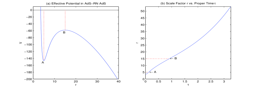
Figure 3: An example of the junction between RN AdS and AdS with multiple accelerations

Again, the possible motions of the wall can be classified by the similar procedures as in the previous cases of Sec. 3. Here we only concentrate on a solution which can behave like experiencing a multi-acceleration phase. From the form of the induced metric on the wall, we may regard $r(\tau)$ as a scale factor. Let the initial radius of the wall be $r_{0}$. Refer to Fig. (3). When time goes on, the wall will expand. As the radius of the wall approaches a point A at $r=5$, the scale factor behaves as $r\approx\tau$ and the first acceleration, the so-called early inflation, ends. After that, the expansion rate of the wall will be decelerated during some time. After the wall goes over the point B at $r=15$, the secondary acceleration will occur and the scale factor be given by

$$r\simeq\exp\left\{\frac{1}{2}\chi_{D}\sqrt{\mid\alpha\mid}\tau\right\}$$ (64)

at $\tau=\infty$.

5 Conclusions and Discussions

In this paper, we classified all possible cosmological behaviors from the viewpoint of an observer on the domain wall moving in 5-dimension. The wall plays a role of a partition that separates the whole manifold into two bulks $M_{\pm}$ and acts on each bulk as a boundary. The junction equation describes the motion of the wall in the radial coordinate and can be interpreted as an equation for the energy conservation of a classical particle under the special potential. Physically, this equation is related with the cosmology of the domain wall because the coordinate $r$ is considered as a scale factor of the metrics of the wall.

It is not clear whether the outside bulk metric can take the form of SAdS in true-false vacuum junction. Hence, we considered only false-true vacuum junctions. The classifications were possible from the shapes of the effective potential depending on the parameter combinations $\alpha$ and $\beta$. From the equation $dV/dr=0$, the extremal points were given by the solution of the quadratic equations of $r_{c}^{D}$. As an example of these, we considered M-SAdS and AdS-SAdS types in detail and their classifications were given by dividing the involved parameter spaces into the corresponding regions. For the dS-S, dS-SdS and dS-AdS junctions, we can get the junction equations by a judicious choice of the parameters.

Finally, we considered a possibility whether solutions with two or more accelerations could exist and found out a special example in the AdS-RN AdS junctions numerically. Without the full classification, we obtained the solution with the late time acceleration as well as the early time inflation. The reason why this was possible was roughly due to the existence of the several extremal points. Since many parameters are used, the positions and the times of the inflations may be adjusted safely. Given a junction, if the effective potential of the problem has many extremal points, it will be possible for a model in the junction to give rise to multiple accelerations.

Acknowledgement We thank E. J. Weinberg for his valuable discussion. This work was supported by the Science Research Center Program of the Korea Science and Engineering Foundation through the Center for Quantum Spacetime(CQUeST) of Sogang University with grant number R11 - 2005 - 021.

References

-
[1]
A. G. Riess et al. [Supernova Search Team Collaboration],
“Observational Evidence from Supernovae for an Accelerating Universe and a
Cosmological Constant,”
Astron. J. 116, 1009 (1998)
[arXiv:astro-ph/9805201].
S. Perlmutter et al. [Supernova Cosmology Project Collaboration], “Measurements of Omega and Lambda from 42 High-Redshift Supernovae,” Astrophys. J. 517, 565 (1999) [arXiv:astro-ph/9812133].
J. L. Tonry et al. [Supernova Search Team Collaboration], “Cosmological Results from High-z Supernovae,” Astrophys. J. 594, 1 (2003) [arXiv:astro-ph/0305008].
-
[2]
A. T. Lee et al.,
“A High Spatial Resolution Analysis of the MAXIMA-1 Cosmic Microwave
Background Anisotropy Data,”
Astrophys. J. 561, L1 (2001)
[arXiv:astro-ph/0104459].
C. B. Netterfield et al. [Boomerang Collaboration], “A measurement by BOOMERANG of multiple peaks in the angular power spectrum of the cosmic microwave background,” Astrophys. J. 571, 604 (2002) [arXiv:astro-ph/0104460].
N. W. Halverson et al., “DASI First Results: A Measurement of the Cosmic Microwave Background Angular Power Spectrum,” Astrophys. J. 568, 38 (2002) [arXiv:astro-ph/0104489].
D. N. Spergel et al. [WMAP Collaboration], “First Year Wilkinson Microwave Anisotropy Probe (WMAP) Observations: Determination of Cosmological Parameters,” Astrophys. J. Suppl. 148, 175 (2003) [arXiv:astro-ph/0302209]. -
[3]
S. Coleman, Phys. Rev. D15,
2929 (1977); ibid. D16, 1248(E) (1977).
C. G. Callan and S. Coleman, Phys. Rev. D16, 1762 (1977). - [4] S. Coleman and F. De Luccia, Phys. Rev. D21, 3305 (1980).
- [5] S. Parke, Phys. Lett. B121, 313 (1983).
- [6] K. Lee and E. J. Weinberg, Phys. Rev. D36, 1088 (1987).
-
[7]
Y. Kim, K. i. Maeda and N. Sakai,
“Monopole-Bubble in Early Universe,”
Nucl. Phys. B 481, 453 (1996)
[arXiv:gr-qc/9604030].
Y. Kim, S. J. Lee, K. i. Maeda and N. Sakai, “Gauged monopole-bubble,” Phys. Lett. B 452, 214 (1999) [arXiv:hep-ph/9901436]. - [8] J. C. Hackworth and E. J. Weinberg, “Oscillating bounce solutions and vacuum tunneling in de Sitter spacetime,” Phys. Rev. D 71, 044014 (2005) [arXiv:hep-th/0410142].
- [9] W. Lee, B.-H. Lee, C. H. Lee, and C. Park, “The False vacuum bubble nucleation due to a nonminimally coupled scalar field,” Phys. Rev. D74, 123520 (2006) [arXiv:hep-th/0604064].
- [10] E. Farhi and A. H. Guth, Phys. Lett. B183, 149 (1987).
- [11] S. K. Blau, E. I. Guendelman, and A. H. Guth, Phys. Rev. D35, 1747 (1987).
- [12] A. Aguirre and M. C. Johnson, “Dynamics and instability of false vacuum bubbles,” Phys. Rev. D 72, 103525 (2005) [arXiv:gr-qc/0508093].
- [13] . Freivogel, V. E. Hubeny, A. Maloney, R. Myers, M. Rangamani and S. Shenker, “Inflation in AdS/CFT,” JHEP 0603, 007 (2006) [arXiv:hep-th/0510046].
- [14] G. L. Alberghi, D. A. Lowe and M. Trodden, “Charged false vacuum bubbles and the AdS/CFT correspondence,” JHEP 9907, 020 (1999) [arXiv:hep-th/9906047].
- [15] L. Randall and R. Sundrum, “A large mass hierarchy from a small extra dimension,” Phys. Rev. Lett. 83, 3370 (1999) [arXiv:hep-ph/9905221].
- [16] L. Randall and R. Sundrum, “An alternative to compactification,” Phys. Rev. Lett. 83, 4690 (1999) [arXiv:hep-th/9906064].
-
[17]
C. Park and S. J. Sin,
“Moving domain walls in AdS(5) and graceful exit from inflation,”
Phys. Lett. B 485, 239 (2000)
[arXiv:hep-th/0005013].
N. Kaloper,
“Bent domain walls as braneworlds,”
Phys. Rev. D 60, 123506 (1999)
[arXiv:hep-th/9905210].
T. Nihei, “Inflation in the five-dimensional universe with an orbifold extra dimension,” Phys. Lett. B 465, 81 (1999) [arXiv:hep-ph/9905487].
H. B. Kim and H. D. Kim, “Inflation and gauge hierarchy in Randall-Sundrum compactification,” Phys. Rev. D 61, 064003 (2000) [arXiv:hep-th/9909053].
C. Csaki, M. Graesser, C. F. Kolda and J. Terning, “Cosmology of one extra dimension with localized gravity,” Phys. Lett. B 462, 34 (1999) [arXiv:hep-ph/9906513].
P. J. Steinhardt, “General considerations of the cosmological constant and the stabilization of moduli in the brane-world picture,” Phys. Lett. B 462, 41 (1999) [arXiv:hep-th/9907080].
O. DeWolfe, D. Z. Freedman, S. S. Gubser and A. Karch, “Modeling the fifth dimension with scalars and gravity,” Phys. Rev. D 62, 046008 (2000) [arXiv:hep-th/9909134].
P. Kanti, I. I. Kogan, K. A. Olive and M. Pospelov, “Cosmological 3-brane solutions,” Phys. Lett. B 468, 31 (1999) [arXiv:hep-ph/9909481].
D. J. H. Chung and K. Freese, “Can geodesics in extra dimensions solve the cosmological horizon problem?,” Phys. Rev. D 62, 063513 (2000) [arXiv:hep-ph/9910235].
J. M. Cline, C. Grojean and G. Servant, “Cosmological expansion in the presence of extra dimensions,” Phys. Rev. Lett. 83, 4245 (1999) [arXiv:hep-ph/9906523].
S. S. Gubser, “AdS/CFT and gravity,” Phys. Rev. D 63, 084017 (2001) [arXiv:hep-th/9912001].
P. Binetruy, C. Deffayet, U. Ellwanger and D. Langlois, Phys. Lett. B 477, 285 (2000) [arXiv:hep-th/9910219].
D. Ida, “Brane-world cosmology,” JHEP 0009, 014 (2000) [arXiv:gr-qc/9912002].
D.J. Chung and K. Freese, Phys. Rev. D61 (2000) 023511, [hep-ph/9906542].
C. Csaki, M. Graesser, L. Randall and J. Terning, “Cosmology of brane models with radion stabilization,” Phys. Rev. D 62, 045015 (2000) [arXiv:hep-ph/9911406].
A. Mazumdar and J. Wang, “A note on brane inflation,” Phys. Lett. B 490, 251 (2000) [arXiv:gr-qc/0004030].
H. Collins and B. Holdom, “Brane cosmologies without orbifolds,” Phys. Rev. D 62, 105009 (2000) [arXiv:hep-ph/0003173].
R. N. Mohapatra, A. Perez-Lorenzana and C. A. de Sousa Pires, “Cosmology of brane-bulk models in five dimensions,” Int. J. Mod. Phys. A 16, 1431 (2001) [arXiv:hep-ph/0003328].
L. Mersini-Houghton, “Decaying cosmological constant of the inflating branes in the Randall-Sundrum-Oda model,” Mod. Phys. Lett. A 16, 1933 (2001) [arXiv:hep-ph/9909494].
L. Mersini-Houghton, “Radion potential and brane dynamics,” Mod. Phys. Lett. A 16, 1583 (2001) [arXiv:hep-ph/0001017].
R. Maartens, D. Wands, B. A. Bassett and I. Heard, “Chaotic inflation on the brane,” Phys. Rev. D 62, 041301 (2000) [arXiv:hep-ph/9912464].
E. E. Flanagan, S. H. H. Tye and I. Wasserman, “Cosmological expansion in the Randall-Sundrum brane world scenario,” Phys. Rev. D 62, 044039 (2000) [arXiv:hep-ph/9910498].
E. E. Flanagan, S. H. H. Tye and I. Wasserman, “Cosmological expansion in the Randall-Sundrum brane world scenario,” Phys. Rev. D 62, 044039 (2000) [arXiv:hep-ph/9910498]. - [18] P. Kraus, “Dynamics of anti-de Sitter domain walls,” JHEP 9912, 011 (1999) [arXiv:hep-th/9910149].
- [19] G. D. Birkhoff,“Relativity and Modern Physics,” Harvard Univ. Press, Cambridge (1923)
- [20] G. W. Gibbons and S. W. Hawking, “Action Integrals And Partition Functions In Quantum Gravity,” Phys. Rev. D 15, 2752 (1977).
- [21] H. A. Chamblin and H. S. Reall, “Dynamic dilatonic domain walls,” Nucl. Phys. B 562, 133 (1999) [arXiv:hep-th/9903225].