![[Uncaptioned image]](/html/hep-th/0701193/assets/x1.png)
Split fermion quasi-normal modes
Abstract
In this paper we use the conformal properties of the spinor field to show how we can obtain the fermion quasi-normal modes for a higher dimensional Schwarzschild black hole. These modes are of interest in so called split fermion models, where quarks and leptons are required to exist on different branes in order to keep the proton stable. As has been previously shown, for brane localized fields, the larger the number of dimensions the faster the black hole damping rate. Moreover, we also present the analytic forms of the quasi-normal frequencies in both the large angular momentum and the large mode number limits.
pacs:
02.30Gp, 03.65geI Introduction
With the advent of theories postulating the existence of additional dimensions, there has been much discussion in the literature related to the quasi-normal modes (QNMs) of black holes (BHs), for example, in the context of the QNMs of higher dimensional BHs see reference HiQNM . By QNMs we refer to the complex frequency modes of oscillation which arise from perturbations of the BH, where the real part represents the actual frequency of the oscillation and the imaginary part represents the damping due to the emission of gravitational waves.
Recent investigations of large extra-dimensional scenarios ADD , where the hierarchy problem can be shifted into a problem of the scale of the extra-dimensions, has led to the somewhat striking prediction that BHs may be observed at particle accelerators such as the LHC BHacc , for an interesting treatment of mini BHs within an effective field theory framework see BH4 . However, one poignant problem is that in order to suppress a rapid proton decay we need to physically split the quarks and leptons. Such models are generically called split fermions models, see, for example, reference Split . In supersymmetric versions of this idea the localizing scalars and bulk gauge fields will have fermionic bulk superpartners. In this respect it is important to consider the properties of bulk fermions. Note that up to now only brane localized QNMs have been calculated BraneQNMs (where other BH effects have been considered in reference Stojkovic ).
That said, the motivations for studying the fermion QNMs from BHs in this paper are two-fold; the first of these being from the theoretical point of view, where the lack of any work done in greater than four dimensions Cho2 with Dirac fields is an omission in the literature. Our calculations serve to fill this gap. Secondly, having a complete catalog of all QNMs would be a necessary precursor to eventually studying the emission rates of collider produced, or TeV scale, BHs. In a forthcoming work we shall present details of BH absorption cross-sections for bulk Schwarzschild fermions in -dimensions Forth . See also reference Dai for tense branes in six-dimensions, where bulk fermions on the tense brane background defined there have yet to be obtained.
As such, this paper shall be structured as follows: In the next section we shall discuss how a conformal transformation of the metric allows for a convenient separation of the Dirac equation into a time-radial part and a -sphere, in -dimensions. Such a method has already been applied in reference Das to the case of low energy -wave absorption cross-sections (which the authors are currently generalizing to higher energies and quantum numbers). However, this has not been used yet in the context of BH QNMs. After this we shall present our results for the QNMs, along with the analytical forms of the frequencies in both the large angular momentum as well as the large mode number limits. Finally, in the last section, we shall make some concluding statements.
II Spinor radial wave equation
We shall begin our analysis by supposing a background metric which is -dimensional and spherically symmetric, as given by:
| (1) |
where denotes the metric for the -dimensional sphere.
Under a conformal transformation Das ; Gibbons :
| (2) | |||||
| (3) | |||||
| (4) |
where we shall take , the metric becomes:
| (5) |
Since the part and the -sphere part of the metric are completely separated, one can write the Dirac equation in the form:
| (6) |
where . Note that from this point on we shall change our notation by omitting the bars.
We shall now let be the eigenspinors for the -sphere Camporesi , that is:
| (7) |
where . Since the eigenspinors are orthogonal, we can expand as:
| (8) |
The Dirac equation can thus be written in the form:
| (9) |
which is just a -dimensional Dirac equation with a interaction.
To solve this equation we make the explicit choice of the Dirac matrices:
| (10) |
where the are the Pauli matrices:
| (11) |
Also,
| (12) |
The spin connections are then found to be:
| (13) |
From this point on we shall work with the sign solution, where the sign case would work in the same way. The Dirac equation can then be written explicitly as:
| (14) |
We shall now determine solutions of the form:
| (15) |
where is the energy. The Dirac equation can then be simplified to:
| (16) |
or
| (17) | |||||
| (18) |
It will be convenient to define the tortoise coordinate, , and the function as:
| (19) |
In which case, our equations can be expressed as:
| (20) |
The equations can then be separated to give:
| (21) |
where:
| (22) |
Since and are supersymmetric to each other, and will have the same spectra, both for scattering and quasi-normal. Incidentally, for , we have these two potentials again.
Refining our study now to a -dimensional Schwarzschild BH, where becomes:
| (23) |
and where the horizon is at with:
| (24) |
In this case the potential can be expressed as:
| (25) | |||||
Next, we shall define, for notational convenience:
| (26) | |||||
| (27) |
with . This allows the above potential, , to be simplified to:
| (28) |
For the case , this then becomes:
| (29) |
with , which is just the radial equation for the Dirac equation in the 4-dimensional Schwarzschild BH Cho .
III QNMs Using The Iyer and Will Method
| Odd | |||
|---|---|---|---|
| =0, n=0 | 0.725 - 0.396 i | 1.79 - 0.809 i | 2.66 - 0.999 i |
| =1, n=0 | 1.32 - 0.384 i | 2.73 - 0.807 i | 3.73 - 1.03 i |
| =1, n=1 | 1.15 - 1.22 i | 2.05 - 2.68 i | 2.30 - 3.57 i |
| =2, n=0 | 1.88 - 0.384 i | 3.61 - 0.817 i | 4.71 - 1.06 i |
| =2, n=1 | 1.75 - 1.18 i | 3.11 - 2.56 i | 3.65 - 3.35 i |
| =2, n=2 | 1.56 - 2.03 i | 2.27 - 4.53 i | 1.80 - 6.23 i |
| =3, n=0 | 2.43 - 0.384 i | 4.46 - 0.821 i | 5.64 - 1.08 i |
| =3, n=1 | 2.33 - 1.17 i | 4.08 - 2.52 i | 4.85 - 3.29 i |
| =3, n=2 | 2.17- 1.99 i | 3.38 - 4.36 i | 3.30 - 5.84 i |
| =3, n=3 | 1.96 - 2.84 i | 2.46 - 6.36 i | 1.30 - 8.87 i |
| Even | |||
| =0, n=0 | 1.28 - 0.639 i | 2.24 - 0.924 i | 3.05 - 1.05 i |
| =1, n=0 | 2.10 - 0.623 i | 3.27 - 0.936 i | 4.14 - 1.10 i |
| =1, n=1 | 1.71 - 2.04 i | 2.24 - 3.18 i | 2.26 - 3.87 i |
| =2, n=0 | 2.87- 0.631 i | 4.21 - 0.956 i | 5.14 - 1.14 i |
| =2, n=1 | 2.11 - 3.42 i | 3.45 - 3.01 i | 3.75 - 3.59 i |
| =2, n=2 | 2.27 - 4.53 i | 2.15 - 5.45 i | 1.26 - 6.95 i |
| =3, n=0 | 3.61 - 0.632 i | 5.11 - 0.964 i | 6.08 - 1.16 i |
| =3, n=1 | 3.39 - 1.93 i | 4.54 - 2.96 i | 5.06 - 3.54 i |
| =3, n=2 | 3.00 - 3.32 i | 3.46 - 5.18 i | 2.95 - 6.340 i |
| =3, n=3 | 2.49 - 4.78 i | 2.04 - 7.69 i | 0.327 - 10.0 i |
To evaluate the QNM frequencies we adopt the WKB approximation developed by Iyer and Will IW , also see references therein. Note that this analytic method has been used extensively in various BH cases Iyer , where comparisons with other numerical results have been found to be accurate up to around 1% for both the real and the imaginary parts of the frequencies for low-lying modes with (where is the mode number and is the spinor angular momentum quantum number). Furthermore, we have also included the modes in our results, but the inclusion of these modes does depend on the number of the dimensions . The formula for the complex quasi-normal mode frequencies in the WKB approximation, carried to third order beyond the eikonal approximation, is given by IW :
| (30) |
where we denote as the maximum of and
| (31) | |||||
| (32) | |||||
Here
| (35) |
It is worth mentioning that in the spin-1/2 case it does not seem possible to solve for for an arbitrary value of , that is, to find an analytic solution for the roots (unlike the case for fields of other spins Iyer ). In the case of a bulk spin-0 field and the graviton tensor perturbations on a -dimensional Schwarzschild background a similar analytic expression can be found for in dimensions, see reference Cornell . Thus, we must find this maximum numerically using a root finding algorithm. Note that for a given we can solve for the roots analytically using a symbolic computer program, although this is not essential, it does improve the performance of our code.
IV Large Angular Momentum
If we now focus on the large angular momentum limit () we can easily extract an analytic expression for the QNMs to first order:
| (36) |
where is the maximum of the potential , see equation (28). In this limit the potential now takes the form:
| (37) |
The location of the maximum of the potential is at
| (38) |
The maximum of the potential in such a limit is then found to be:
| (39) |
In this case we find from the 1st order WKB approximation that:
| (40) |
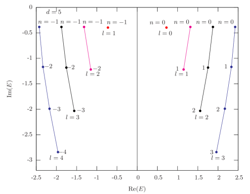
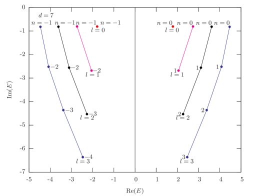
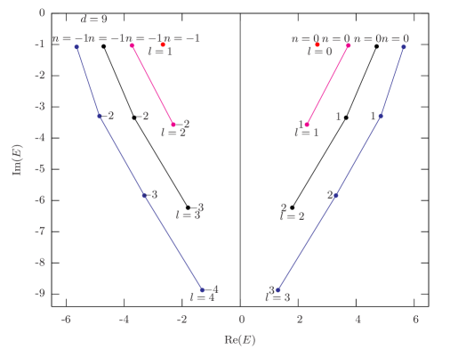
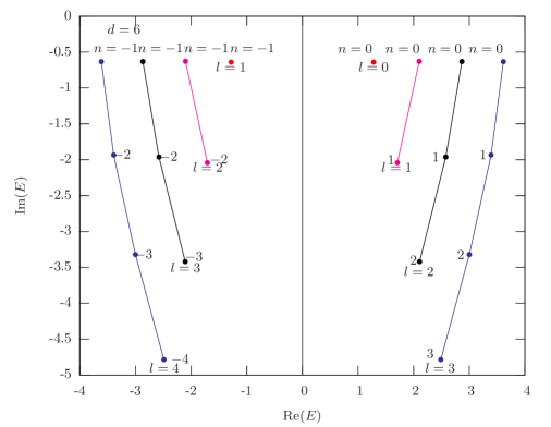
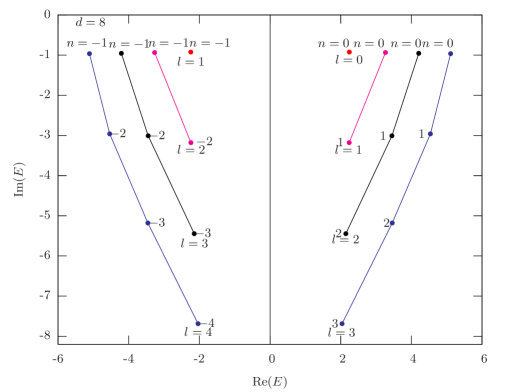
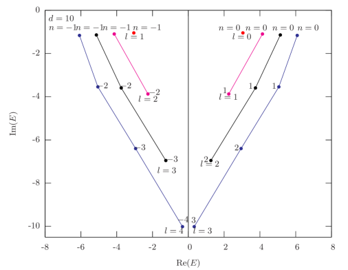
This result agrees with the standard result in four dimensions, , for example see reference Iyer , and is similar to the spin-0 result given in reference Konoplya . These limiting values also appear to agree well with the plots made in Figure 1 and 2. We have also plotted the QNM dependence on dimension, , in Figure 3.
V Asymptotic quasinormal frequency
Finally, we can also calculate the quasinormal frequency in the limit of large mode number, . In this case, as we can see from the results in the previous sections, that as the imaginary part of tends to negative infinity, . Hence, we are really looking at the large limit here. Using the method by Andersson and Howls Andersson , who have combined the WKB formalism with the monodromy method of Motl and Neitzke Motl , we make our evaluations in this limit. Note that in reference Cho2 this method has been used to obtain the asymptotic quasinormal frequency for the four-dimensional Dirac field. Since we are following the same procedure as in references Cho2 ; Andersson , we shall only show the essential steps, where one can consult references Cho2 ; Andersson for details. To start we return to equation (21):
| (41) |
Defining a new function,
| (42) |
equation (41) can be rewritten as:
| (43) |
with
| (44) |
The WKB solutions to this equation are:
| (45) |
where is a reference point and
| (46) | |||||
As , the zeros of , or the turning points, , in this WKB approximation, are close to the origin in the complex -plane. In this limit,
| (47) |
and the turning points are at:
| (48) |
Asymptotically is very close to the negative imaginary axis, that is, , as such, the turning points can then be represented by:
| (49) |
for . Note that the equation giving the asymptotic quasinormal frequency involves two quantities, the first being the line integral from one turning point to the other. Here, we have:
| (50) | |||||
where we have made the change of variable . The other quantity is the closed contour integration around :
| (51) |
The asymptotic quasinormal frequency is then given by the formula,
| (52) | |||||
for large . In terms of the corresponding Hawking temperature, ,
| (53) |
We therefore obtain a vanishing real part for the frequency and find that the spacing of the imaginary part goes to regardless of the dimension. Note that these results are in accordance with that of integral spin fields in higher-dimensional Schwarzschild spacetimes Motl ; SDas ; Natario .
VI Concluding remarks
In this paper we have presented new results for the QNMs of a massless Dirac field on a bulk -dimensional background, see Figure 1 and 2. The results can be compared with the brane-localized results of reference BraneQNMs , revealing that bulk fermion modes result in much larger damping rates (in both cases larger results in greater damping rates). Some words of caution are necessary, as can be seen for example in the result, which plots the and channels. In the next angular momentum channel, , the point , crosses the imaginary axis. The presence of a branch cut along this axis would force us to choose the positive imaginary value in accordance with the constraint equation (35). However this does not signify that there are modes which are unstable, but indicates, as can be deduced from our asymptotic large analysis, that the WKB approximation is breaking down.
Furthermore, if a more detailed analysis such as along the lines of Leaver’s approach Leaver confirms the result that some of the QNMs have real part equal to zero (algebraically special frequencies), as our WKB results imply for , then such modes would be transparent. However, as mentioned, we cannot say too much based upon the WKB approximation in this vicinity.
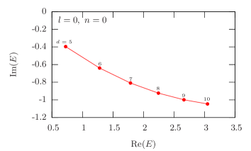
Also, given that the BH damping rate increases with dimension , see Figure 3, we can naively infer that the amount of energy available to be radiated as Hawking radiation will increase with . These issues are left for further study Forth .
In section IV we investigated the large angular momentum limit and found an asymptotic result that agrees with the result. In section V we discussed the remaining issue of asymptotic quasinormal frequencies. The expected result in -dimensions is obtained in such a limit. Note that recently Dirac QNMs have been analyzed under the influence of Lorentz violation Chen . It is of interest that the authors introduce a term in their equations similar to the one found in our reduced 2-dimensional Dirac equation (9).
Finally, it may be worth mentioning that split fermion theories often have massive fermions in the bulk, examples of this are the higher order modes of the quarks and leptons, which are freed from the localizing potential at high energy. Other examples are the bulk Higginos and gauginos in SUSY formulations. In addition to our results, depending on the energy scale involved, investigations of these massive Dirac QNMs would also be of interest.
Acknowledgments
HTC was supported in part by the National Science Council of the Republic of China under the Grant NSC 95-2112-M-032-013. JD wishes to thank Dr. G. C. Joshi for his advice and supervision during the production of this work. The authors would also like to thank Prof. Misao Sasaki for the guidance and advice given during the many fruitful discussions we had with him.
References
- (1) R. A. Konoplya, Phys. Rev. D 68 (2003) 124017 [arXiv:hep-th/0309030]; E. Berti, M. Cavaglia and L. Gualtieri, Phys. Rev. D 69 (2004) 124011 [arXiv:hep-th/0309203]; V. Cardoso, J. P. S. Lemos and S. Yoshida, Phys. Rev. D 69 (2004) 044004 [arXiv:gr-qc/0309112]; V. Cardoso, J. P. S. Lemos and S. Yoshida, JHEP 0312 (2003) 041 [arXiv:hep-th/0311260]; V. Cardoso, G. Siopsis and S. Yoshida, Phys. Rev. D 71 (2005) 024019 [arXiv:hep-th/0412138]; D. K. Park, Phys. Lett. B 633 (2006) 613 [arXiv:hep-th/0511159]; A. Lopez-Ortega, Gen. Rel. Grav. 38 (2006) 1747 [arXiv:gr-qc/0605034]; R. G. Daghigh, G. Kunstatter, D. Ostapchuk and V. Bagnulo, Class. Quant. Grav. 23 (2006) 5101 [arXiv:gr-qc/0604073]; F. W. Shu and Y. G. Shen, JHEP 0608 (2006) 087 [arXiv:hep-th/0605128]; J. y. Shen, B. Wang and R. K. Su, Phys. Rev. D 74 (2006) 044036 [arXiv:hep-th/0607034]; Sayan K. Chakrabarti, Kumar S. Gupta Int.J.Mod.Phys. A21 (2006) 3565-3574.
- (2) H. T. Cho, Phys. Rev. D 73 (2006) 024019 [arXiv:gr-qc/0512052].
- (3) N. Arkani-Hamed, S. Dimopoulos and G. R. Dvali, Phys. Lett. B 429, 263 (1998).
- (4) P. C. Argyres, S. Dimopoulos and J. March-Russell, Phys. Lett. B 441, 96 (1998); S. Dimopoulos and G. Landsberg, Phys. Rev. Lett. 87, 161602 (2001); S. B. Giddings and S. D. Thomas, Phys. Rev. D 65, 056010 (2002).
- (5) S. Bilke, E. Lipartia, and M. Maul, [arXiv:hep-ph/0204040]; S.R. Choudhury, A.S. Cornell, G.C. Joshi, and B.H.J. McKellar, Mod. Phys. Lett. A 19, 2331 (2004), [arXiv:hep-ph/0307275]; Jason Doukas, S.R. Choudhury and G.C. Joshi, Mod. Phys. Lett. A 21, 2561 (2006), [arXiv:hep-ph/0604220];
- (6) N. Arkani-Hamed and M. Schmaltz, Phys. Rev. D 61, 033005 (2000); N. Arkani-Hamed, Y. Grossman and M. Schmaltz, Phys. Rev. D 61, 115004 (2000); T. Han, G. D. Kribs and B. McElrath, Phys. Rev. Lett. 90, 031601 (2003);
- (7) D. C. Dai, G. D. Starkman and D. Stojkovic, Phys. Rev. D 73, 104037 (2006); D. Stojkovic, F. C. Adams and G. D. Starkman, Int. J. Mod. Phys. D 14, 2293 (2005).
- (8) P. Kanti and R. A. Konoplya, Phys. Rev. D 73 (2006) 044002 [arXiv:hep-th/0512257]; P. Kanti, R. A. Konoplya and A. Zhidenko, Phys. Rev. D 74 (2006) 064008 [arXiv:gr-qc/0607048].
- (9) H. T. Cho, A. S. Cornell, J. Doukas, W. Naylor and M. Sasaki, work in progress.
- (10) D. C. Dai, N. Kaloper, G. D. Starkman and D. Stojkovic, [arXiv:hep-th/0611184].
- (11) S. R. Das, G. W. Gibbons and S. D. Mathur, Phys. Rev. Lett. 78 (1997) 417 [arXiv:hep-th/9609052].
- (12) G. W. Gibbons and A. R. Steif, Phys. Lett. B 314 (1993) 13 [arXiv:gr-qc/9305018].
- (13) R. Camporesi and A. Higuchi, J. Geom. Phys. 20 (1996) 1 [arXiv:gr-qc/9505009].
- (14) H. T. Cho, Phys. Rev. D 68 (2003) 024003 [arXiv:gr-qc/0303078].
- (15) S. Iyer and C. M. Will, Phys. Rev. D 35 (1987) 3621.
- (16) S. Iyer, Phys. Rev. D 35 (1987) 3632.
- (17) R. A. Konoplya, Phys. Rev. D 68 (2003) 024018 [arXiv:gr-qc/0303052].
- (18) A. S. Cornell, W. Naylor and M. Sasaki, JHEP 0602 (2006) 012 [arXiv:hep-th/0510009].
- (19) N. Andersson and C. J. Howls, Class. Quantum Grav. 21 (2004) 1623 [arXiv:gr-qc/0307020].
- (20) L. Motl and A. Neitzke, Adv. Theor. Math. Phys. 7 (2003) 307 [arXiv:hep-th/0301173].
- (21) S. Das and S. Shankaranarayanan, Class. Quantum Grav. 22 (2005) L7 [arXiv:hep-th/0410209].
- (22) J. Natario and R. Schiappa, Adv. Theor. Math. Phys. 8 (2004) 1001 [arXiv:hep-th/0411267].
- (23) E. W. Leaver, Proc. Roy. Soc. Lond. A 402 (1985) 285.
- (24) Songbai Chen, Bin Wang, Rukeng Su, [arXiv:gr-qc/0701089]