The energy absorption problem of a brane-world black hole

Abstract

We have studied the wave dynamics and the energy absorption problem for the scalar field as well as the brane-localized gravitational field in the background of a braneworld black hole. Comparing our results with the four-dimensional Schwarzschild black hole, we have observed the signature of the extra dimension in the energy absorption spectrum.

I Introduction

Recent developments on higher dimensional gravity resulted in a number of interesting theoretical ideas such as the brane-world concept in which the standard model fields are confined to our four-dimensional world viewed as a hyperspace embedded in the higher-dimensional spacetime where gravity can propagates1 ; randall ; s3 . The simplest models in this context are proposed by Randall and Sundrumrandall . It was argued that the extra dimensions need not be compact and in particular it was shown that it is possible to localize gravity on a 3-brane when there is one infinite extra dimension s1 ; randall . A striking consequence of the theory with large extra dimensions is that it can lower the fundamental gravity scale and allow the production of mini black holes in the universe. Such mini black holes are centered on the brane and may have been created in the early universe due to density perturbations and phase transitions. Recently it was proposed that such mini black holes may also be produced in high energy collisions and could be probed in particle accelerator experiments in the very near futures4 ; s5 ; s6 ; s7 .

A great deal of effort has been expanded for the precise determination of observational signatures of such mini black holes. One among them is the black hole quasinormal modes (QNM), which can disclose the evolution of the perturbation around black hole during a certain time interval and was argued carrying unique fingerprint of the black hole existence and is expected to be detected through gravitational wave observations in the near future (see reviews on this topic and references therein s8 ). Recently the QNMs of a brane-world black hole have been studied in eabdalla ; abdalla ; shen . The gravitational perturbation of the mini black hole would be a characteristic sound and could tell us the existence of such black hole. Another chief possibility of observing this kind of mini black hole is the spectrum of Hawking radiation which is expected to be detected in particle accelerator experiments s9 ; s10 ; s11 ; s14 ; s12 ; park ; shen ; Horowitz2 ; park2 ; kaloper2 . Since such small black holes carry information of extra dimensions and persist different properties compared to those of ordinary 4-dimensional black holes, these two tools of detecting mini black holes can help to read the extra dimensions.

Most of the available works have been done for the idealized case by studying the brane-localized modes in the QNM and Hawking radiation. One of the reason is that in the brane world scenario it was assumed that most standard matter fields are brane-localized. In the study of Hawking radiation, it was argued that the emission on the brane is dominated compared to that off the braneHorowitz . This argument was supported numerically in the case of standard model field emission by the (4 + n)-dimensional non-rotating black holes s12 ; park and also in the higher-dimensional rotating black hole backgroundHorowitz2 . Some counterexamples to this argument have also been foundpark2 . However in general it is very hard to obtain exact soltions of higher-dimensional Einstein equations so that the knowledge of the bulk is lacking, the thorough study on the field emission in the bulk is still a challenging task. Using a recently constructed exact black hole localized on a 3-brane in a world with two large extra dimensions kaloper , Dai et al explored the Hawking decay channels with the influence of the brane tensionkaloper2 . They found for the non-rotating black holes the dominate channels are still the brane-localized modes.

In this paper we are going to study a braneworld black hole obtained in casadio . A general class of spherically symmetric and static solution to the field equation with a 5-dimensional cosmological constant can be derived by considering a general line element of the type

$$ds^{2}=A(r)dt^{2}-\frac{1}{B(r)}dr^{2}-r^{2}d\Omega^{2},$$ (1)

and relaxing the condition $A(r)=B^{-1}(r)$ used in obtaining the usual 4-dimensional black holes. Casadio et al obtained two types of solutions by fixing either $A(r)$ or $B(r)$ and in one case with the choice $A(r)=1-2M/r$, the metric reads casadio

$$ds^{2}=(1-\frac{2M}{r})dt^{2}-\frac{1-\frac{3M}{2r}}{\left(1-\frac{2M}{r}\right)\left(1-\frac{\gamma M}{2r}\right)}dr^{2}-r^{2}d\Omega^{2}.$$ (2)

This braneworld black hole is called CFM black hole. It would be noted that Eq.(2) was not derived from 5-dimensional solution, but rather was obtained as a solution to 4-dimensional equations constraining the possible form of the 5-dimensional metric. The extension of the asymptotically flat static spherically metric on the brane into the bulk has been discussed in dd . The usual 4-dimensional Schwarzschild black hole is recovered with $\gamma=3$. The corresponding Hawking temperature is given bycasadio $T_{BH}=\sqrt{1-3(\gamma-3)/2}/(8\pi M)$. Thus in comparison with the Schwarzschild black hole, the braneworld black hole will either be hotter or colder depending upon the sign of $\gamma-3$. In this work we are restricted to the case when $\gamma\leq 11/3$ as in eabdalla to ensure the Hawking temperature to be physical. The QNM of this kind of braneworld black hole was studied in eabdalla . We will concentrate on the absorption problem of this black hole. Immersed in external radiation fields, the black hole scatters the radiation and may either absorb or amplify it. The process is described by dynamical perturbation equations in the black hole background. We will study the scalar and axial gravitational perturbations on the background of this CFM black hole and investigate the absorption problem. We will extract the information on the extra dimensional influence on the absorption of the braneworld black hole by comparing to that of the usual four-dimensional black hole.

For future convenience, we adopt the notation in Ch ,

$$ds^{2}=e^{2\nu}dt^{2}-e^{2\psi}d\varphi^{2}-e^{2\mu_{2}}dr^{2}-e^{2\mu_{3}}d\theta^{2}.$$ (3)

Comparing with (2), we have

$$e^{2\nu}=A(r),\ \ e^{-2\mu_{2}}=B(r),\ \ e^{2\mu_{3}}=r^{2},\ \ e^{2\psi}=r^{2}\sin^{2}\theta.$$ (4)

In the vicinity of the event horizon $r_{H}$, the asymptotic expressions of the metric components $A(r)$ and $B(r)$ can be written in the first order

$$A(r)\sim A_{1}(r/r_{H}-1),$$

$$B(r)\sim B_{1}(r/r_{H}-1),\ \ (r\rightarrow r_{H}+0),$$ (5)

where $A_{1}=1$ and $B_{1}=4-\gamma$ are dimensionless, positive real numbers. Demanding that the spacetime is asymptotically flat, we have,

$$A(r)\rightarrow 1,$$ (6)

$$B(r)\rightarrow 1,\ \ (r\rightarrow\infty).$$

Our paper is organized as follows: in §II we will go over scalar perturbation and investigate its energy absorption; in §III we will derive the wave equation of the gravitational perturbation and study its energy absorption spectra. We will sumarize our results in the last section.

II Scalar Perturbation and Its energy Absorption

For simplicity we first consider the braneworld black hole immersed in the massless scalar field confined on the brane. We will go over the scalar perturbation and study the energy absorption problem in the general four dimensional spherical metric, Eq. (1) and then apply the general results to the CFM black hole.

II.1 Scalar Perturbation Equations

The scalar perturbation is governed by the Klein-Gorden equation. For the massless scalar field, we have

$$\Box\Phi=(-g)^{-1/2}\partial_{\mu}\left[(-g)^{1/2}g^{\mu\nu}\partial_{\nu}\Phi\right]=0.$$ (7)

Using the decomposition of the scalar field

$$\Phi=\sum_{l=0}^{\infty}R_{l}(r)P_{l}(\cos\theta)e^{-i\omega t},$$ (8)

we have the Schrödinger like radial wave equations,

$$\frac{d^{2}(rR_{l})}{dr_{*}^{2}}+\left[\omega^{2}-V_{s,l}(r)\right](rR_{l})=0.$$ (9)

$r_{*}$ is the tortoise coordinate defined as $dr_{*}=dr/\sqrt{AB}$. The effective potential reads

$$V_{s,l}=A\frac{l(l+1)}{r^{2}}+\frac{1}{2r}\left(A^{\prime}B+AB^{\prime}\right).$$ (10)

II.2 Boundary Conditions

There are freedoms in choosing boundary conditions depending on physical pictures of different problems. We will consider the plane wave scattering in our work.

II.2.1 Boundary Condition at Infinity

In the remote region, by virtue of the scattering problem, the scalar field at infinity is in the form

$$\Phi\sim\left[e^{i\omega r\cos\theta}+\frac{f(\theta)}{r}e^{i\omega r}\right]e^{-i\omega t}.$$ (11)

Referring to the scheme of partial wave method in quantum mechanics, the plane wave can be expanded into spherical waves as,

$$e^{i\omega r\cos\theta}=\sum_{l=0}^{\infty}(2l+1)i^{l}j_{l}(\omega r)P_{l}(\cos\theta).$$ (12)

When $r$ tends to infinity,

$$e^{i\omega r\cos\theta}\sim\sum_{l=0}^{\infty}(-1)^{l+1}\frac{2l+1}{2\omega r}[e^{-i\omega r}-(-1)^{l}e^{i\omega r}]P_{l}(\cos\theta).$$ (13)

The scattered wave can also be expanded in the form

$$\frac{f(\theta)}{r}e^{i\omega r}=\sum_{l=0}^{\infty}(2l+1)f^{s}_{l}\frac{e^{i\omega r}}{2\omega r}P_{l}(\cos\theta),$$ (14)

where $f^{s}_{l}$ are complex constants, and the superscript ”s” indicates the case of scalar field. Inserting this equation together with Eq. (13) into Eq. (11), we have the boundary condition at infinity

$$\Phi\sim e^{-i\omega t}\sum_{l=0}^{\infty}(-1)^{l+1}\frac{2l+1}{2\omega r}[e^{-i\omega r_{*}}-(-1)^{l}S^{s}_{l}e^{i\omega r_{*}}]P_{l}(\cos\theta),$$ (15)

where $S^{s}_{l}=1+f^{s}_{l}$, and the radius $r$ on the exponentials are replaced by tortoise coordinate $r_{*}$ for future convenience. Note that at infinity $dr_{*}\sim dr$ so that such replacement on the exponentials makes no difference. In accordance, we have the boundary condition of $R_{l}$ at infinity

$$R_{l}\sim(-1)^{l+1}\frac{2l+1}{2\omega r}[e^{-i\omega r_{*}}-(-1)^{l}S^{s}_{l}e^{i\omega r_{*}}].$$ (16)

II.2.2 Boundary Condition at Horizon

Now we examine the boundary condition in the near-horizon region. We can express the solution of Eq. (9) in power series persides

$$R_{l}=(r/r_{H}-1)^{\rho}\sum_{n=0}^{\infty}d_{l,n}(r/r_{H}-1)^{n}.$$ (17)

In the vicinity of the horizon, we have the asymptotic behavior

$$\sqrt{AB}\sim\sqrt{A_{1}B_{1}}(r/r_{H}-1),$$ (18)

as well as

$$V_{s,l}(r)\sim O(r-r_{H}),\ \ \ (r\rightarrow r_{H}+0).$$ (19)

Inserting the expansions Eq. (18,19) into the radial equation Eq. (9), we have

$$A_{1}B_{1}[\rho(\rho-1)+\rho]+r_{H}^{2}\omega^{2}=0,$$ (20)

or,

$$\rho=\pm\frac{i\omega r_{H}}{\sqrt{A_{1}B_{1}}}.$$ (21)

Since nothing can escape from the black hole, only the minus sign is acceptable. Thus we have the boundary condition of $R_{l}(r)$ near the horizonpersides

$$R_{l}(r)\sim g_{l}(r/r_{H}-1)^{-i\omega r_{H}/\sqrt{A_{1}B_{1}}},$$ (22)

where $g_{l}$ are the zero-th coefficient of the expansion of $R_{l}$: $g_{l}=d_{l,0}$, which is dimensionless. The boundary condition for the total perturbational scalar field $\Phi$ is given by

$$\Phi\sim e^{-i\omega t}\sum_{l=0}^{\infty}g_{l}(r/r_{H}-1)^{-i\omega r_{H}/\sqrt{A_{1}B_{1}}}P_{l}(\cos\theta).$$ (23)

II.3 The Energy Flux and the Absorption Cross Section

The energy flux is derived from the energy-momentum tensor of the scalar field. For massless scalar field, it is generally expressed as early9

$$T_{\mu\nu}=\Phi_{;\mu}\Phi^{*}_{;\nu}-\frac{1}{2}g_{\mu\nu}\Phi^{;\alpha}\Phi^{*}_{;\alpha}.$$ (24)

The energy-momentum flow of the spacetime is defined byearly4

$$P^{\mu}=T^{\mu}_{\nu}\xi^{\nu}(t),$$ (25)

where vector $\xi(t)=\partial/\partial t$ is the time-like Killing vector. We now calculate the energy falling into the black hole per unit time using Gauss’ theorem. In the theorem, for any appropriate four vector $A^{\mu}$ and space time sector $\mathcal{N}$, there holds

$$\int_{\mathcal{N}}A^{\mu}_{;\mu}\mathbf{\Omega}_{4}=\int_{\partial\mathcal{N}}A^{\mu}n_{\mu}\mathbf{\Omega}_{3},$$ (26)

where $\mathbf{\Omega_{4}}$ and $\mathbf{\Omega_{3}}$ are the volume elements of the spacetime sector $\mathcal{N}$, and its boundary $\partial\mathcal{N}$. $n^{\mu}$ is the normal vector of the boundary $\partial\mathcal{N}$ which satisfies $\hat{\mathbf{n}}\wedge\mathbf{\Omega}_{3}=\mathbf{\Omega}_{4}$, where $\hat{\mathbf{n}}$ is the 1-form physically equivalent to vector $n^{\mu}$. Here we may choose the space time sector $\mathcal{N}$ to be the spacial area within two spheres of radius $r_{1}$ and $r_{2}$, and with the time interval between $t_{1}$ and $t_{2}$, whose boundaries are $\partial\mathcal{N}$. To find out the energy falling into the hole, we focus on the hypersurface of $r=r_{1}$, whose normal vector is $n_{\mu}=(0,\sqrt{A/B},0,0)$, and we let $r_{1}\rightarrow r_{H}$. Thus the energy falling into the hole within the time interval between $t_{1}$ and $t_{2}$ is Ch ,

$$E^{(abs)}=\int^{t_{2}}_{t_{1}}dt\int_{4\pi}P^{\mu}n_{\mu}r_{H}^{2}\sin\theta d\theta d\varphi=\int^{t_{2}}_{t_{1}}dt\int_{4\pi}T_{0\mu}n^{\mu}r_{H}^{2}\sin\theta d\theta d\varphi.$$ (27)

Applying the explicit forms of $T_{0\mu}$ and $n^{\mu}$, as well as the boundary condition Eq. (23), we have, at the horizon

$$T_{0\mu}n^{\mu}=-\sqrt{AB}\ \partial_{t}\Psi\partial_{r}\Psi^{*}|_{r_{H}}=\omega^{2}\left|\sum_{l=0}^{\infty}g_{l}P_{l}(\cos\theta)\right|^{2}.$$ (28)

Inserting this into Eq. (27), we have the total energy falling into the horizon per unit time:

$$\Phi^{(abs)}=\frac{dE^{(abs)}}{dt}=4\pi\omega^{2}r_{H}^{2}\sum_{l=0}^{\infty}\frac{|g_{l}|^{2}}{2l+1}.$$ (29)

Here, we have used the orthogonality of Legendre polynomials,

$$\int_{-1}^{1}{P_{l}(x)P_{l^{\prime}}(x)dx}=\frac{\delta_{ll^{\prime}}}{2l+1}.$$ (30)

On the other hand, following the similar procedure as above, we can derive the expression of the energy flux of the incoming wave at infinity, which is simply

$$j^{(inc)}=\omega^{2}.$$ (31)

Therefore for the massless scalar wave the total energy absorption by the black hole is given by

$$\sigma^{abs}_{s}=\frac{\Phi^{(abs)}}{j^{(inc)}}=4\pi r_{H}^{2}\sum_{l=0}^{\infty}\frac{|g_{l}|^{2}}{2l+1}.$$ (32)

For angular index $l$, the partial absorption cross section is expressed as

$$\sigma_{s,l}^{abs}=4\pi r_{H}^{2}\frac{|g_{l}|^{2}}{2l+1}.$$ (33)

After we get $g_{l}$ we can obtain the final result of the absorption spectrum.

For the radial equation Eq. (9), the Wronskians for any two solutions $R_{l}^{(1)}$ and $R_{l}^{(2)}$ is

$$W[R_{l}^{(1)},R_{l}^{(2)}]=\frac{K_{12}}{r^{2}\sqrt{AB}},$$ (34)

with the constant $K_{12}$ to be determined by the explicit form of the two solutions. Using the asymptotic solution of $R_{l}$ at infinity Eq. (16), we have

$$W[R_{l}^{*},R_{l}]=-\frac{i(2l+1)^{2}}{2\omega r^{2}\sqrt{AB}}\left(1-|S^{s}_{l}|^{2}\right),$$ (35)

and employing the asymptotic solution at the horizon Eq. (22), we get

$$W[R_{l}^{*},R_{l}]=-\frac{2i\omega r_{H}^{2}}{r^{2}\sqrt{AB}}|g_{l}|^{2}.$$ (36)

Equating the above two equations, we find

$$|g_{l}|^{2}=\frac{(2l+1)^{2}}{4\omega^{2}r_{H}^{2}}\left(1-|S^{s}_{l}|^{2}\right).$$ (37)

Thus with Eq. (33) we can express the energy absorption in the form

$$\sigma^{abs}_{s,l}=\frac{\pi}{\omega^{2}}(2l+1)\Gamma^{s}_{l},$$ (38)

where $\Gamma^{s}_{l}$ is defined in terms of $S^{s}_{l}$ as

$$\Gamma^{s}_{l}=1-|S_{l}^{s}|^{2}.$$ (39)

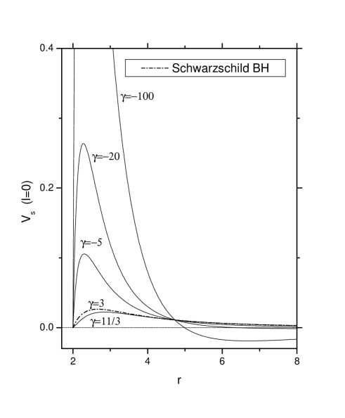
Figure 1: The effective potential of the scalar perturbation with the change of $\gamma$ and $l$.

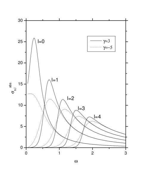
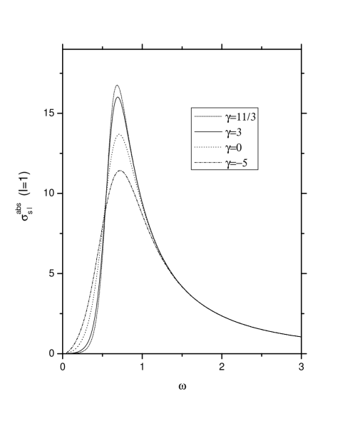
Figure 2: The partial energy absorption of the scalar wave with the change of $\gamma,l$

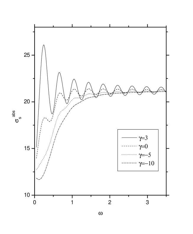
Figure 3: The total energy absorption of the scalar wave.

II.4 Numerical Study for the Scalar Perturbation

Now we proceed to calculate numerically the coefficients $g_{l}$. Instead of solving Eq. (9) directly for $R_{l}$, we choose the particular solution $\varphi_{l}(r)$, normalized as

$$\varphi_{l}(r)=g_{l}^{-1}R_{l}(r).$$ (40)

In the asymptotically flat region, it resolves into outgoing and ingoing waves

$$\varphi_{l}(r)=f_{l}^{(-)}\mathcal{F}_{l(+)}+f_{l}^{(+)}\mathcal{F}_{l(-)},$$ (41)

wherepark ; persides

$$\mathcal{F}_{l(\pm)}=e^{\mp i\omega r_{*}}\sum_{n=0}^{\infty}\tau^{(\pm)}_{l,n}\left(\frac{r_{H}}{r}\right)^{n+1},$$ (42)

satisfying $\mathcal{F}_{l(+)}=\mathcal{F}_{l(-)}^{*}$ and the coefficients $\tau_{l,0}^{(\pm)}$ being unity for simplicity. The combination coefficients $f_{l}^{(\pm)}$ are called jost functions. Comparing this to Eq. (16), we have

$$g_{l}=\frac{(-1)^{l+1}}{\omega}\frac{l+1/2}{f_{l}^{(-)}},$$ (43)

$$S_{l}^{s}=(-1)^{l+1}\frac{f_{l}^{(+)}}{f_{l}^{(-)}}.\ \ \$$ (44)

Thus if the jost functions are known, we can get the solution to our problem. Applying Eq. (34) to the two particular solutions at infinity, we have

$$W[\mathcal{F}_{l(+)},\mathcal{F}_{l(-)}]=\frac{2i\omega r_{H}^{2}}{r^{2}\sqrt{AB}},$$ (45)

and therefore we have the jost functions

$$f_{l}^{(\pm)}=\mp W[\varphi_{l},\mathcal{F}_{l(\pm)}]\frac{r^{2}\sqrt{AB}}{2i\omega r_{H}^{2}}.$$ (46)

In numerical calculation, we would like to express $g_{l}$ in Eq. (32) and Eq. (33) in terms of the jost functions, and the absorption cross section therefore reads

$$\sigma^{abs}_{s,l}=\frac{\pi}{\omega^{2}}\frac{2l+1}{|f_{l}^{(-)}|^{2}},$$ (47)

and

$$\sigma^{abs}_{s}=\frac{\pi}{\omega^{2}}\sum_{l=0}^{\infty}\frac{2l+1}{|f_{l}^{(-)}|^{2}}.$$ (48)

We now report our numerical result for the massless scalar perturbation in the CFM braneworld black hole background. Inserting the metric components into Eq. (10), the effective potential has the form

$$V_{s,l}(r)=\left(1-\frac{2M}{r}\right)\left[\frac{l(l+1)}{r^{2}}+\frac{2M}{r^{3}}+\frac{M(\gamma-3)(r^{2}-6Mr+6M^{2})}{r^{3}(2r-3M)^{2}}\right].$$ (49)

Taking $M=1$, the bahavior of the potential is shown in Fig.1. We see that there is a potential barrier outside the horizon and for the fixed angular index $l$ this barrier increases for more negative $\gamma$. Fixing $\gamma$, we find that the potential barrier increases with the increase of the angular index. When $\gamma$ becomes small, the potential has a negative well after the positive barrier. The negative well appears earlier for very negative $\gamma$. This was also observed in eabdalla . Comparing with the height of the positive barrier, the absolute value of the negative peak is very small for chosen $\gamma$. Thus the potential barrier will dominate in the determination of the wave dynamics, which qualitatively leads to the general quasinormal ringing as disclosed in eabdalla .

The spectrum of absorption cross sections for both Schwarzschild and the brane-world case with $\gamma=-5$ are shown in Fig.2a for different $l$. Fig.2b displays the partial absorption cross section for chosen $l$ and different $\gamma$. It is noticed that the absorption cross section of the brane-world black hole can be either smaller or larger than that in the Schwarzschild black hole provided that $\gamma$ is smaller or bigger than $3$. This result is consistent with the behavior of the potential barriers as shown in Fig.1. The higher or lower barrier of the potential could decrease or increase the absorption of the scalar field around the brane-world black hole. For the low $\omega$ region, we observed that the absorption is higher for smaller values of $\gamma$. This could be the imprint of the negative well in the potential, since different from the barrier, the potential well enhances the absorption rate. But the overall behavior of the energy absorption shows that the potential barrier dominates the physics.

In Fig.3, we show the spectrum of the total absorption cross section, we see that with the decrease of $\gamma$, there are fewer oscillations. For smaller $\gamma$, in the low energy band the total absorptions are suppressed. This is because of the increase in the potential barrier which plays the dominate role for smaller $\gamma$ leading to the decrease of the absorption of the incoming wave. The full penetration occurs when the incoming wave with very high energy, which explains why the total absorption approaches a constant value at high frequency.

III Gravitational Perturbation and Its Energy Absorption Cross Section

Now we start the formulation of gravitational perturbation, of which the detailed deduction requires special techniques provided in Ch ; a1 . We will concentrate our attention here on the brane-localized axial perturbation in the background of the braneworld black hole.

III.1 Axial Gravitational Perturbation Equations

Using the formalism introduced in Ch , the axially perturbed metric Eq. (1) is

$$ds^{2}=e^{2\nu}(dt)^{2}-e^{2\psi}(d\varphi-\varpi dt-q_{2}dx^{2}-q_{3}dx^{3})^{2}-e^{2\mu_{2}}(dx^{2})^{2}-e^{2\mu_{3}}(dx^{3})^{2}.$$ (50)

Here

$$x^{2}=r,\ \ x^{3}=\theta,$$ (51)

$\varpi$ and $q_{i}\ (i=2,3)$ are quantities that embody the perturbation. Due to the lack of knowledge of the 5D bulk metric, we restrict to the brane localized perturbation governed by the perturbation equation

$$\delta R_{\mu\nu}=0.$$ (52)

This simplification is supported by the analysis of gravitational shortcuts abdalla2 which shows that gravitational fields do not travel deep into the bulk. It can be justified at least in a regime where the perturbation energy does not exceed the threshold of the Kaluza-Klein massive modes. By defining

$$Q_{ij}=q_{i},_{j}-q_{j},_{i},\ \ Q_{0i}=\varpi,_{i}-q_{i},_{0},$$ (53)

one finds equations

$$(e^{3\psi+\nu-\mu_{2}-\mu_{3}}Q_{23}),_{3}=-e^{3\psi-\nu+\mu_{3}-\mu_{2}}Q_{02},_{0}$$ (54)

from $\delta R_{12}=0$, and

$$(e^{3\psi+\nu-\mu_{2}-\mu_{3}}Q_{23}),_{2}=e^{3\psi-\nu+\mu_{2}-\mu_{3}}Q_{03},_{0}$$ (55)

from $\delta R_{13}=0$. We take

$$e^{3\psi+\nu-\mu_{2}-\mu_{3}}Q_{23}=r^{2}\sqrt{AB}\sin^{3}\theta Q_{23}=Q$$ (56)

in Eq. (54) and Eq. (55), and then cancel $\varpi$, to arrive at an equation of $Q$:

$$-r^{2}\frac{\partial^{2}Q}{\partial t^{2}}+r^{4}\sqrt{AB}\frac{\partial}{\partial r}\left(\frac{\sqrt{AB}}{r^{2}}\frac{\partial Q}{\partial r}\right)+A\sin^{3}\theta\frac{\partial}{\partial\theta}\left(\frac{1}{\sin^{3}\theta}\frac{\partial Q}{\partial\theta}\right)=0.$$ (57)

Analogously, this equation plays the same role as the Klein-Gorden equation in the scalar perturbation. However the equation here cannot be separated in terms of Legendre polynomials as in the Klein-Gorden equation, the Gegenbauer polynomials are employed to carry out the separationCh . $Q$ is now seperated as

$$Q(t,r,\theta)=\sum_{l=2}^{\infty}rZ_{l}(r)C^{-3/2}_{l+2}(\cos\theta)e^{-i\omega t},$$ (58)

where the Gegenbauer polynomials $C^{-3/2}_{l+2}(\theta)$ satisfy the equation

$$\sin^{2\nu}\theta\frac{d}{d\theta}\left(\sin^{-2\nu}\theta\frac{dC^{\nu}_{l}(\cos\theta)}{d\theta}\right)+l(l+2\nu)C^{\nu}_{l}(\cos\theta)=0.$$ (59)

The radial Schrödinger-like equation can be derived in the form,

$$\frac{d^{2}Z_{l}}{dr_{*}^{2}}+[\omega^{2}-V_{g,l}(r)]Z_{l}=0.$$ (60)

$r_{*}$ is the tortoise coordinate defined by $dr_{*}=dr/\sqrt{AB}$, and the effective potential is

$$V_{g,l}(r)=A\frac{(l-1)(l+2)}{r^{2}}+\frac{2AB}{r^{2}}-\frac{A^{\prime}B+B^{\prime}A}{2r}.$$ (61)

III.2 Boundary Conditions

We set the boundary conditions to be those of plane wave scattering.

III.2.1 Boundary Condition at Infinity

It is expected that the quantity $Q=r^{2}\sqrt{AB}\sin^{3}\theta Q_{23}$ has the similar behavior of the scattered spherical wave since a straightforward examination shows that $Q(t,r,\theta)=e^{i(\omega r\cos\theta-\omega t)}$ is exactly a solution of Eq. (57) in the region far from the black hole. Therefore it is appropriate to write

$$Q(t,r,\theta)\sim\left[e^{i\omega r\cos\theta}+\frac{f(\theta)}{r}e^{i\omega r}\right]e^{-i\omega t},\ \ r\rightarrow\infty.$$ (62)

For the infinite $r$, $Q$ behaves as Eq. (62), which can also be expanded in a combination of Gagenbauer polynomials as the decomposition of $Q$ in Eq. (58). The expansion of the plane wave part is ToI

$$e^{i\omega r\cos\theta}=-\frac{1}{3}\sum_{l=-2}^{\infty}(l+1/2)i^{l}(\omega r)^{2}j_{l}(\omega r)C^{-3/2}_{l+2}(\cos\theta).$$ (63)

Note that in practice we calculate only the partial absorption cross section of low angular indices, thus when $\omega r$ is a large number, the asymptotic approximation for $j_{l}(\omega r)$ reads

$$j_{l}(x)\sim\frac{1}{x}\sin(x-l\pi/2)=-\frac{i^{l}}{2x}\left[e^{-ix}-(-1)^{l}e^{ix}\right]$$ (64)

for $x\gg 1$ and $x\gg l$, where $x=\omega r$. There exists a certain $l_{0}$ and before this $l_{0}$ the summation terms of Eq. (63) may be replaced by the asymptotic form,

$$e^{i\omega r\cos\theta}=\frac{1}{6}\sum_{l=-2}^{l_{0}}(l+1/2)(-1)^{l}(\omega r)\left[e^{-i\omega r}-(-1)^{l}e^{i\omega r}\right]C^{-3/2}_{l+2}(\cos\theta)$$

$$+\left[-\frac{1}{3}\sum_{l=l_{0}+1}^{\infty}(l+1/2)i^{l}(\omega r)^{2}j_{l}(\omega r)C^{-3/2}_{l+2}(\cos\theta)\right].\ \ \ \ \ \$$ (65)

The larger $\omega r$ is, the larger $l_{0}$ will be.

We also need the expansion of the term representing the scattered wave. Formally we may write

$$\frac{f(\theta)}{r}e^{ikr}=\sum_{l=-2}^{\infty}\chi_{l}(r)C^{-3/2}_{l+2}(\cos\theta).$$ (66)

Similar to the plane wave, we expect that before some integer $l_{0}^{\prime}$, the summation coefficients in Eq. (66) are asymptotically

$$\chi_{l}(r)\sim\frac{1}{6}(l+1/2)(\omega r)f^{g}_{l}e^{i\omega r},$$ (67)

at some very large $\omega r$, where $f^{g}_{l}$ are complex numbers depending solely on index $l$. Thus we can write the expansion Eq. (66) as

$$\frac{f(\theta)}{r}e^{i\omega r}=\frac{1}{6}\sum_{l=-2}^{l_{0}^{\prime}}(l+1/2)(\omega r)f^{g}_{l}e^{i\omega r}C_{l+2}^{-3/2}(\cos\theta)$$

$$+\sum_{l=l_{0}^{\prime}+1}^{\infty}\chi_{l}(r)C^{-3/2}_{l+2}(\cos\theta).\ \ \ \ \ \ \$$ (68)

Combining Eq. (III.2.1) and Eq. (III.2.1), we have the applicable form of the asymptotic behavior of $Q(t,r,\theta)$:

$$Q\sim\frac{e^{-i\omega t}}{6}\sum_{l=2}^{\min(l_{0},l_{0}^{\prime})}(l+1/2)(-1)^{l}(\omega r)\left[e^{-i\omega r}-(-1)^{l}S^{g}_{l}e^{i\omega r}\right]C^{-3/2}_{l+2}(\cos\theta)+\ldots.$$ (69)

Here the omitted terms are those over the upper limit for applying the asymptotic form, which are not applicable to our numerical calculation. $S^{g}_{l}=1-f^{g}_{l}$ is a complex number being the ratio of incoming and outgoing wave. The summation starts from index 2 for the modes from $l=-2$ to $l=1$ are not physical in gravitational perturbation. Since $\min(l_{0},l_{0}^{\prime})$ certainly exceeds our need for numerical calculation, we may write for simplicity

$$Q\sim\frac{e^{-i\omega t}}{6}\sum_{l=2}^{\infty}(l+1/2)(-1)^{l}(\omega r)\left[e^{-i\omega r_{*}}-(-1)^{l}S^{g}_{l}e^{i\omega r_{*}}\right]C^{-3/2}_{l+2}(\cos\theta),$$ (70)

which is valid for a limited number of angular indices. As done in the scalar case, in the exponentials we have replaced $r$ into $r_{*}$, since in the remote region the spacetime is flat and we actually have $dr_{*}\sim dr$. Therefore the boundary condition for $Z_{l}(r)$ at infinity reads

$$Z_{l}(r)\sim\frac{1}{6}(l+1/2)(-1)^{l}\omega\left[e^{-i\omega r_{*}}-(-1)^{l}S^{g}_{l}e^{i\omega r_{*}}\right]\ \ r\rightarrow\infty.$$ (71)

III.2.2 Boundary Condition at the Horizon

We now study the boundary condition in the vicinity of the event horizon $r_{H}$. Expanding $Z_{l}(r)$ near the horizonpersides

$$Z_{l}(r)=\left(\frac{r}{r_{H}}-1\right)^{\rho}\sum_{n=0}^{\infty}c_{l,n}\left(\frac{r}{r_{H}}-1\right)^{n},$$ (72)

we have

$$\frac{dZ_{l}}{dr}\sim\frac{p_{l}\rho}{r_{H}}\left(\frac{r}{r_{H}}-1\right)^{\rho-1},\ \ \ \ \frac{d^{2}Z_{l}}{dr^{2}}\sim\frac{p_{l}\rho(\rho-1)}{r_{H}^{2}}\left(\frac{r}{r_{H}}-1\right)^{\rho-2},$$ (73)

when $r\rightarrow r_{H}$. $p_{l}=c_{l,0}$ with the dimension of length^-1. Considering Eq.(18), in the vicinity of the event horizon Eq. (73) becomes

$$\frac{d^{2}Z_{l}}{dr_{*}^{2}}\sim A_{1}B_{1}\left(\frac{r}{r_{H}}-1\right)^{2}\frac{d^{2}Z_{l}}{dr^{2}}+\frac{A_{1}B_{1}}{r_{H}}\left(\frac{r}{r_{H}}-1\right)\frac{dZ_{l}}{dr}\sim\frac{p_{l}\rho^{2}(A_{1}B_{1})}{r_{H}}\left(\frac{r}{r_{H}}-1\right)^{\rho},$$ (74)

and

$$[\omega^{2}-V_{eff}(r)]Z_{l}\sim p_{l}\omega^{2}\left(\frac{r}{r_{H}}-1\right)^{\rho}.$$ (75)

Inserting Eq. (74) and Eq. (75) into Eq. (60), we obtain

$$A_{1}B_{1}[\rho(\rho-1)+\rho]+r_{H}^{2}\omega^{2}=0,$$ (76)

where

$$\rho=\pm i\omega r_{H}/\sqrt{A_{1}B_{1}}.$$ (77)

Similar to the scalar case, we choose the minus sign in the $\rho$ expression since there is only ingoing wave near the event horizon and nothing can escape from the black hole. The boundary condition at the horizon then reads

$$Z_{l}(r)\sim p_{l}(r/r_{H}-1)^{-i\omega r_{H}/\sqrt{A_{1}B_{1}}},\ \ r\rightarrow r_{H}+0.$$ (78)

In accordance the behavior of $Q(t,r,\theta)$ at the horizon is

$$Q(t,r,\theta)\sim e^{-i\omega t}r_{H}(r/r_{H}-1)^{-i\omega r_{H}/\sqrt{A_{1}B_{1}}}\sum_{l=2}^{\infty}p_{l}C^{-3/2}_{l+2}(\cos\theta)\ ,\ \ r\rightarrow r_{H}+0.$$ (79)

III.3 Application of the Newman-Penrose Formalism

The study of the gravitational perturbation and the gravitational energy absorption spectrum involves considerable algebraic complexity. There is a well developed approach to this problem provided by Teukolsky early4 ; early9 , where Newman-Penrose formalism was employed. In this section we will employ the formalism to calculate the energy flux coming from infinity and the energy falling into the black hole.

III.3.1 Formalism in the Kinnersley Tetrad

This tetrad serves to calculate the incoming energy flux of the gravitational wave at infinityKin . It is set to be

$$l^{\mu} = \frac{1}{A}(1,\sqrt{AB},0,0),$$ (80)

$$n^{\mu} = \frac{1}{2}(1,-\sqrt{AB},0,0),$$ (81)

$$m^{\mu} = \frac{1}{\sqrt{2}r}(0,0,1,i\csc\theta),$$ (82)

of which the components queue in the order $(t,r,\theta,\varphi)$. The corresponding spin coefficients are found to be

$$\kappa=\sigma=\lambda=\nu=\epsilon=\pi=\tau=0,\ \ \ \ \ \ \ \ \ \ \ \ \ \ \ \ \$$ (83)

$$\rho=\frac{1}{r}\sqrt{\frac{B}{A}},\ \alpha=-\beta=\frac{\cot\theta}{2\sqrt{2}r},\ \mu=\frac{\sqrt{AB}}{2r},\ \gamma=\frac{A_{,r}}{4}\sqrt{\frac{B}{A}}.$$ (84)

Here, taking $A=B$ recovers the Schwarzschild case.

Then we need to evaluate two contractions of the perturbation of the Riemann tensor with the Kinnersley tetrad, which play key roles in calculating the energy flux at infinity and the energy falling down the hole, and which hereafter is denoted by $\tilde{\Psi}_{0}^{(1)}$ and $\tilde{\Psi}_{4}^{(1)}$, defined as

$$\tilde{\Psi}_{0}^{(1)}=-\delta R_{\mu\nu\lambda\sigma}l^{\mu}m^{\nu}l^{\lambda}m^{\sigma},$$ (85)

and

$$\tilde{\Psi}_{4}^{(1)}=-\delta R_{\mu\nu\lambda\sigma}n^{\mu}m^{\nu*}n^{\lambda}m^{\sigma*}.$$ (86)

To perform the contraction a new orthonormal tetrad was introduced

$$e^{\mu}_{(0)} = (e^{-\nu},0,0,0),$$ (87)

$$e^{\mu}_{(1)} = (0,e^{-\psi},0,0),$$ (88)

$$e^{\mu}_{(2)} = (0,0,e^{-\mu_{2}},0),$$ (89)

$$e^{\mu}_{(3)} = (0,0,0,e^{-\mu_{3}}),$$ (90)

where components are ordered by $(x^{0},x^{1},x^{2},x^{3})=(t,\varphi,r,\theta)$. The components of Kinnersley tetrad against this tetrad basis are therefore

$$l^{(\mu)} = (e^{-\nu},0,e^{-\nu},0),$$ (91)

$$n^{(\mu)} = \frac{1}{2}(e^{\nu},0,-e^{\nu},0),$$ (92)

$$m^{(\mu)} = \frac{1}{\sqrt{2}}(0,i,0,1).$$ (93)

Here the indices in the bracket indicate the components against the basis of Eq. (87) through Eq. (90), and they run through 0 to 3. Now we do the contraction of Eq. (85) and find

$$\tilde{\Psi}_{0}^{(1)}= - ie^{-2\nu}(\delta R_{0301}+\delta R_{2321}+\delta R_{2301}+\delta R_{0321})$$ (94)

$$-\frac{1}{2}e^{-2\nu}(\delta R_{0303}+2\delta R_{0323}+\delta R_{2323}-\delta R_{0101}-2\delta R_{0121}-\delta R_{2121}),$$

as well as

$$\tilde{\Psi}_{4}^{(1)}= - \frac{i}{4}e^{2\nu}(-\delta R_{0301}-\delta R_{2321}+\delta R_{2301}+\delta R_{0321})$$ (95)

$$-\frac{1}{8}e^{2\nu}(\delta R_{0303}-2\delta R_{0323}+\delta R_{2323}-\delta R_{0101}+2\delta R_{0121}-\delta R_{2121}).$$

Here, in both expressions, the second bracket would vanish in purely axial perturbation, whose demonstration was raised in §31 of Ch and applicable to all static, spherically symmetric metric. For convenience, we denote the non-vanishing part, which contains the first bracket, of Eq. (94) and Eq. (95) to be $i\ \textrm{Im}\tilde{\Psi}_{0}^{(1)}$ and $i\ \textrm{Im}\tilde{\Psi}_{4}^{(1)}$, and the vanishing part, $\textrm{Re}\tilde{\Psi}_{0}^{(1)}$ and $\textrm{Re}\tilde{\Psi}_{4}^{(1)}$. The Riemann components therein can be simplified as (§13 of Ch ),

$$\delta R_{0301} = \frac{1}{2}e^{\psi-2\nu-\mu_{3}}Q_{03,0}-\frac{1}{2}e^{\psi-2\mu_{2}-\mu_{3}}Q_{23}\nu_{,r}\ ,$$ (96)

$$\delta R_{2321} = e^{\psi-2\mu_{2}-\mu_{3}}\left[\left(\frac{1}{r}-\frac{1}{2}\mu_{2,r}\right)Q_{23}+\frac{1}{2}Q_{23,r}\right],$$ (97)

$$\delta R_{2301} = \frac{1}{2}e^{\psi-\nu-\mu_{2}-\mu_{3}}\left[Q_{03,2}-Q_{02,3}+Q_{03}\left(\frac{1}{2}+\mu_{2,r}\right)-Q_{02}\cot\theta\right],$$ (98)

$$\delta R_{0321} = -\frac{1}{2}e^{\psi-\nu-\mu_{2}-\mu_{3}}\left[Q_{20,3}+Q_{20}\cot\theta-Q_{23,0}+Q_{30}\left(\frac{1}{r}-\nu_{,r}\right)\right].$$ (99)

Inserting these equations into Eq. (94) and Eq. (95), we have

$$-\frac{e^{2\nu+2\mu_{2}}}{\sin\theta}\textrm{Im}\tilde{\Psi}_{0}^{(1)}=\frac{Q_{23}}{r}+\frac{1}{2}Q_{23,r}+\frac{1}{2}e^{-\nu+\mu_{2}}Q_{23,0}-\frac{1}{2}(\mu_{2,r}+\nu_{,r})Q_{23}$$

$$+\frac{1}{2}e^{-\nu+\mu_{2}}\left[Q_{03,r}+\left(\frac{2}{r}-\nu_{,r}+\mu_{2,r}\right)Q_{03}\right]+\frac{1}{2}e^{-2\nu+2\mu_{2}}Q_{03,0},$$ (100)

and

$$-\frac{4e^{-2\nu+2\mu_{2}}}{\sin\theta}\textrm{Im}\tilde{\Psi}_{4}^{(1)}=-\frac{Q_{23}}{r}-\frac{1}{2}Q_{23,r}+\frac{1}{2}e^{-\nu+\mu_{2}}Q_{23,0}+\frac{1}{2}(\mu_{2,r}+\nu_{,r})Q_{23}$$

$$+\frac{1}{2}e^{-\nu+\mu_{2}}\left[Q_{03,r}+\left(\frac{2}{r}-\nu_{,r}+\mu_{2,r}\right)Q_{03}\right]-\frac{1}{2}e^{-2\nu+2\mu_{2}}Q_{03,0}.$$ (101)

With the aid of Eq. (54) through Eq. (57), the two contractions can be simplified to be

$$2i\omega\ \textrm{Im}\tilde{\Psi}_{0}^{(1)}=\sum_{l=2}^{\infty}\left\{\left(\frac{2\sqrt{AB}}{r}-\frac{A^{\prime}B+AB^{\prime}}{2\sqrt{AB}}-2i\omega\right)\Lambda_{(-)}Z_{l}+\left[\frac{i\omega(AB^{\prime}-A^{\prime}B)}{2\sqrt{AB}}+V_{g,l}\right]Z_{l}\right\}\frac{C^{-3/2}_{l+2}(\cos\theta)}{rA^{2}\sin^{2}\theta},$$ (102)

and

$$8i\omega\ \textrm{Im}\tilde{\Psi}_{4}^{(1)}=\sum_{l=2}^{\infty}\left\{\left(\frac{2\sqrt{AB}}{r}-\frac{A^{\prime}B+AB^{\prime}}{2\sqrt{AB}}-2i\omega\right)\Lambda_{(+)}Z_{l}+\left[\frac{i\omega(A^{\prime}B-AB^{\prime})}{2\sqrt{AB}}+V_{g,l}\right]Z_{l}\right\}\frac{C^{-3/2}_{l+2}(\cos\theta)}{r\sin^{2}\theta},$$ (103)

where $V_{g,l}$ is the radial effective potential defined by Eq. (61) and $\Lambda_{(\pm)}=d/dr_{*}\pm i\omega$. It is easy to check that equating $A(r)$ and $B(r)$ would recover the result in the Schwarzschild case.

III.3.2 Formalism in the Hawking-Hartle Tetrad

To calculate the gravitational wave energy flux on the horizon, the Kinnersley tetrad is no longer applicable because of their singular behavior at the horizon. We use the tetrad introduced by Hartle and Hawking insteadHH , which represents a physical observer crossing the event horizon. It eliminates the singular behavior by imposing on the Kinnersley tetrad a rotation of the third class (Ch , §8). In our problem the rotation parameter is $\Lambda=2/A$. The tetrad is normalized so that on the basis of coordinate $(v=t+r_{*},r,\theta,\varphi)$, $(l^{HH})^{v}=1$. This results in the Hawking-Hartle basis as follows:

$$(l^{HH})^{\mu} = 1/2(1,\sqrt{AB},0,0),$$ (104)

$$(n^{HH})^{\mu} = (1/A,-\sqrt{B/A},0,0),$$ (105)

and $m^{\mu}$ is unchanged. The components are arranged in the order of $(t,r,\theta,\varphi)$. Changing to the basis of $(\partial_{v},\partial_{r},\partial_{\theta},\partial_{\varphi})$, we have

$$(l^{HH})^{\mu} = (1,\sqrt{AB}/2,0,0),$$ (106)

$$(n^{HH})^{\mu} = (0,-\sqrt{B/A},0,0),$$ (107)

again with $m^{\mu}$ unchanged. Thus we obtain the well-behaved tetrad on the horizon, which is equivalent to a physical observer advancing along the direction $l^{HH}$. Hereafter we perform calculations in this Hawking-Hartle tetrad. We can derive new spin coefficients using their transformation rules under the third class of tetrad rotation (Ch , §8), the one of importance is

$$\epsilon^{HH}=-\frac{1}{2}\Lambda^{-2}D\Lambda=\frac{1}{4}\sqrt{\frac{B}{A}}\frac{dA}{dr},$$ (108)

where $D$ is the differential operator corresponding to the tangent vector $l^{\mu}$. We define

$$\epsilon_{0}=\epsilon^{HH}_{r_{H}}=\left.\frac{1}{4}\sqrt{\frac{B}{A}}\frac{dA}{dr}\right|_{r_{H}}=\frac{\sqrt{A_{1}B_{1}}}{4r_{H}}.$$ (109)

$2\epsilon_{0}$ is the surface gravity of the black hole (Ch , §8). We also need to know that $\kappa$ vanishes globally, ensuring the integral curves of $l^{HH}$ to be null geodesics, and that $\rho^{HH}$ vanishes at the horizon, since

$$\rho^{HH}=\Lambda^{-1}\rho=\frac{\sqrt{AB}}{2r}\longrightarrow 0,\ \ (r\rightarrow r_{H}).$$ (110)

Moreover, we present here two relations needed for calculating the energy falling into the hole. They are obtained with the perturbation effect, where the Hawking-Hartle tetrad is also perturbed so that $l^{HH}$ is the generator of a congruence of null geodesics, and $\kappa$ always stays zero. We start from two Ricci identities under any Newmann-Penrose basis, which are

$$D\sigma-\delta\kappa = \sigma(3\epsilon-\epsilon^{*}+\rho+\rho^{*})+\kappa(\pi^{*}-\tau-3\beta-\alpha^{*})+\Psi_{0},$$ (111)

$$D\rho-\delta^{*}\kappa = (\rho^{2}+|\sigma|^{2})+\rho(\epsilon+\epsilon^{*})-\kappa^{*}\tau-\kappa(3\alpha+\beta^{*}-\pi)+\Phi_{00}$$ (112)

(Ch , §8). Here $\Psi_{0}$ and $\Phi_{00}$ are projections of the Weyl tensor and the Ricci tensor upon the tetrad. Linearizing these two and with the consequence from $\delta R_{\mu\nu}=0$ that $\Phi^{(1)}_{00}=0$, we find, under Hawking-Hartle tetrad,

$$D^{HH}_{r_{H}}\sigma^{HH(1)}_{r_{H}} = 2\epsilon_{0}\sigma^{HH(1)}_{r_{H}}+\left.\Psi^{HH(1)}_{0}\right|_{r_{H}}\ ,$$ (113)

$$D^{HH}_{r_{H}}\rho^{HH(1)} = 2\epsilon_{0}\rho^{HH(1)}.$$ (114)

III.4 Gravitational Wave Energy Absorption

III.4.1 Incoming Energy Flux at Infinity

The general expression for the incoming energy flux is eFlow ; early9 ; Ch

$$\frac{d^{2}E^{(inc)}}{dtd\Omega}=\frac{1}{64\pi\omega^{2}}\lim_{r\rightarrow\infty}r^{2}|\tilde{\Psi}_{0}^{(1)}|^{2},$$ (115)

where $\tilde{\Psi}_{0}^{(1)}$ is defined in Eq. (94). Considering the axial perturbation, we can replace $\tilde{\Psi}_{0}^{(1)}$ by $\textrm{Im}\tilde{\Psi}_{0}^{(1)}$. Taking $r\rightarrow\infty$ in Eq. (102) and taking into account only the incoming wave, we have

$$\textrm{Im}\tilde{\Psi}_{0}^{(1)}\longrightarrow\sum_{l=2}^{\infty}\left(\Lambda_{(-)}Z_{l}^{(inc)}\right)\frac{C_{l+2}^{-3/2}(\cos\theta)}{r\sin^{2}\theta}\ ,\ \ (r\rightarrow\infty).$$ (116)

With the boundary condition at infinity Eq. (71), we have

$$\Lambda_{(-)}Z_{l}^{(inc)}\longrightarrow(-1)^{l+1}i\omega(2l+1)e^{-i\omega r_{*}}/6,\ \ (r\rightarrow\infty).$$ (117)

Inserting Eq. (116), Eq. (117) into Eq. (115) and integrating the flux over all directions, we obtain the total incoming energy per unit time at infinity

$$\Phi^{(inc)}=\int_{4\pi}{\frac{d^{2}E^{(inc)}}{dtd\Omega}\ d\Omega}=\frac{\omega^{2}}{2304\pi}\sum_{l=2}^{\infty}\int_{4\pi}{\left[\frac{C_{l+2}^{-3/2}(\cos\theta)}{\sin^{2}\theta}\right]^{2}d\Omega}=\frac{\omega^{2}}{192}.$$ (118)

The last equality was obtained by using the orthogonality of the Gegenbauer polynomials ToI

$$\int_{-1}^{1}\frac{C_{l+2}^{-3/2}C_{l^{\prime}+2}^{-3/2}}{(1-x^{2})^{2}}dx=\frac{18\ \delta_{ll^{\prime}}}{(2l+1)(l+2)(l+1)l(l-1)},$$ (119)

and the summation

$$\sum_{l=2}^{\infty}\frac{2l+1}{(l+2)(l+1)l(l-1)}=\frac{1}{3}.$$ (120)

III.4.2 Energy Falling into the Hole

Calculating the gravitational wave energy absorption into the black hole is more complicated than that in the scalar case. We will follow Teukolsky’s treatment early9 to deal with this problem.

With Eq. (114), following the procedure presented in Ch , §98, we have the change in the area of the event horizon in the process of perturbation

$$\frac{d^{2}\Sigma}{dvd\Omega}=\frac{r_{H}^{2}}{\epsilon_{0}}|\sigma_{r_{H}}^{HH(1)}|^{2},$$ (121)

where $\Sigma$ denotes the area of event horizon, and the spin coefficient $\epsilon_{0}$ is presented in Eq. (109). The first law of black hole thermodynamics relates the change of the horizon area to the change of the black hole internal energy

$$dE=\frac{\bar{\kappa}}{8\pi}d\Sigma,$$ (122)

where $\bar{\kappa}=2\epsilon_{0}$ is the surface gravity. Thus

$$\frac{d^{2}\Sigma}{dvd\Omega}=\frac{4\pi}{\epsilon_{0}}\frac{d^{2}E^{(abs)}}{dvd\Omega}.$$ (123)

Combining Eq. (122) and Eq. (123), we have

$$\frac{d^{2}E^{(abs)}}{dvd\Omega}=\frac{r_{H}^{2}}{4\pi}|\sigma_{r_{H}}^{HH(1)}|^{2}.$$ (124)

The spin coefficient $\sigma_{r_{H}}^{HH(1)}$ is evaluated in Eq. (113), where

$$D_{r_{H}}^{HH}=\partial_{v}=\partial_{t}\rightarrow-i\omega,$$ (125)

and consequently we get

$$\sigma_{r_{H}}^{HH(1)}=-\frac{\Psi^{HH(1)}_{0}|_{r_{H}}}{i\omega+2\epsilon_{0}}.$$ (126)

Referring to the transformation of Weyl scalars under the rotation of the third class (Ch , §8), we have

$$\Psi^{HH(1)}_{0}=A^{2}\Psi_{0}^{(1)}/4.$$ (127)

Combining Eq. (127), Eq. (126) and Eq. (124), we arrive at

$$\frac{d^{2}E^{(abs)}}{dvd\Omega}=\frac{r_{H}^{2}}{16\pi}\frac{|A^{2}\Psi^{(1)}_{0}|^{2}_{r_{H}}}{4\omega^{2}+A_{1}B_{1}r_{H}^{-2}}.$$ (128)

Now we need to evaluate $\Psi^{(1)}_{0}=-\delta C_{\mu\nu\rho\lambda}l^{\mu}m^{\nu}l^{\rho}m^{\lambda}$,

$$\Psi_{0}^{(1)}= - ie^{-2\nu}(\delta C_{0301}+\delta C_{2321}+\delta C_{2301}+\delta C_{0321})$$ (129)

$$-\frac{1}{2}e^{-2\nu}(\delta C_{0303}+2\delta C_{0323}+\delta C_{2323}-\delta C_{0101}-2\delta C_{0121}-\delta C_{2121}).$$

The Weyl tensors are defined as

$$C_{\mu\nu\rho\lambda}=R_{\mu\nu\rho\lambda}-\frac{1}{2}(g_{\mu\rho}R_{\lambda\nu}-g_{\mu\lambda}R_{\rho\nu}+g_{\nu\rho}R_{\lambda\mu}-g_{\nu\lambda}R_{\rho\mu})+\frac{1}{3}R(g_{\mu\rho}g_{\lambda\nu}-g_{\mu\lambda}g_{\rho\nu}).$$ (130)

Three facts can help greatly simplify the evaluation, which are, (i) only the diagonal components of the Ricci tensor is non-zero for a metric like Eq. (1), (ii) according to the perturbation equation, $\delta R_{\mu\nu}=0$, and (iii) only $\delta g_{1\mu}\neq 0$, $(\mu=0,2,3)$. The evaluation shows that the components of the perturbed Weyl tensors in $\Psi^{(1)}_{0}$ all coincide with those of the Riemann’s, except for $\delta C_{0301}$ and $\delta C_{2321}$, which are

$$\delta C_{0301}=\delta R_{0301}+\frac{1}{2}R_{00}\delta g_{31}+\frac{1}{3}Rg_{00}\delta g_{31},$$ (131)

$$\delta C_{2321}=\delta R_{2321}+\frac{1}{2}R_{22}\delta g_{31}+\frac{1}{3}Rg_{22}\delta g_{31}.$$ (132)

Therefore

$$\Psi^{(1)}_{0}=\tilde{\Psi}^{(1)}_{0}+\frac{ie^{-2\nu}}{2}(R_{00}+R_{22})\delta g_{31}+\frac{ie^{-2\nu}}{3}R(g_{00}+g_{22})\delta g_{31}.$$ (133)

This is further simplified by the fact that we carry out the contraction under the orthonormal basis, Eq. (87) through Eq. (90), where for a spherical metric as Eq. (1) describes, there holds $g_{00}=-g_{22}=1$, implying that $(g_{00}+g_{22})\delta g_{31}\equiv 0$. And also, we have the extended result from the calculation of the Schwarzschild model

$$R_{00}=-\frac{BA^{\prime\prime}}{2A}-\frac{A^{\prime}B^{\prime}}{4A}-\frac{BA^{\prime}}{rA}+\frac{B}{4A^{2}}(A^{\prime})^{2};$$

$$R_{22}=\frac{BA^{\prime\prime}}{2A}+\frac{A^{\prime}B^{\prime}}{4A}+\frac{B^{\prime}}{r}-\frac{B}{4A^{2}}(A^{\prime})^{2},$$ (134)

which gives that

$$R_{00}+R_{22}=\frac{B}{r}(\frac{B^{\prime}}{B}-\frac{A^{\prime}}{A})\sim O(r/r_{H}-1),\ \ (r\rightarrow r_{H}+0).$$ (135)

That is, the term $R_{00}+R_{22}$ is of the first order small quantity as $r$ tends to the horizon. On the other hand, it is easy to check that near the horizon, we have $q_{3,2}\sim Q(r/r_{H}-1)^{-1}\sim(r/r_{H}-1)^{-i(\omega/\sqrt{A_{1}B_{1}})-1}$, so that $\delta g_{31}\sim q_{3}\sim(r/r_{H}-1)^{-i(\omega/\sqrt{A_{1}B_{1}})}$, and hence we have $(R_{00}+R_{22})\delta g_{31}\rightarrow 0$, as $r\rightarrow r_{H}+0$. Therefore in our context

$$\Psi_{0}^{(1)}=i\ \textrm{Im}\tilde{\Psi}_{0}^{(1)}.$$ (136)

Hence

$$\frac{d^{2}E^{(abs)}}{dvd\Omega}=\frac{r_{H}^{2}}{16\pi}\frac{|A^{2}\textrm{Im}\tilde{\Psi}^{(1)}_{0}|^{2}_{r_{H}}}{4\omega^{2}+A_{1}B_{1}r_{H}^{-2}}.$$ (137)

In the vicinity of the event horizon, $r\rightarrow r_{H}+0$, applying the boundary condition Eq. (78), we get

$$A^{2}\textrm{Im}\tilde{\Psi}^{(1)}_{0}\rightarrow\sum_{l=2}^{\infty}\left[\left(\sqrt{A_{1}B_{1}}r_{H}^{-1}-2i\omega\right)\Lambda_{(-)}Z_{l}\right]\frac{C_{l+2}^{-3/2}(\cos\theta)}{2i\omega r_{H}\sin^{2}\theta}\ \ \ \ \ \ \$$

$$\rightarrow-\sum_{l=2}^{\infty}\left[\left(\sqrt{A_{1}B_{1}}r_{H}^{-1}-2i\omega\right)p_{l}(r/r_{H}-1)^{-i\omega r_{H}/\sqrt{A_{1}B_{1}}}\right]\frac{C_{l+2}^{-3/2}(\cos\theta)}{r_{H}\sin^{2}\theta}.$$ (138)

Inserting this expression into Eq. (137) and performing the integration over all directions, we have the total absorbed energy per unit time

$$\Phi^{(abs)} = \int_{4\pi}{\frac{d^{2}E^{(abs)}}{dvd\Omega}\ d\Omega}=\frac{|p_{l}|^{2}}{16\pi}\int_{4\pi}{\left[\frac{C_{l+2}^{-3/2}(\cos\theta)}{\sin^{2}\theta}\right]^{2}d\Omega}.$$ (139)

Employing the orthogonality of the Gagenbauer polynomials, Eq. (138) becomes

$$\Phi^{(abs)}=\frac{9}{4}\sum_{l=2}^{\infty}\frac{|p_{l}|^{2}}{2l+1}\frac{(l-2)!}{(l+2)!}.$$ (140)

III.4.3 The Absorption Cross Section

We define the absorption cross section as the ratio of the total absorbed energy to the total incoming energy at infinity. Averaging the total incident energy over the event horizon, we have the incident energy flux in the analogous sense, that

$$j^{(inc)}=\frac{\Phi^{(inc)}}{4\pi r_{H}^{2}}=\frac{\omega^{2}}{1536\pi r_{H}^{2}}.$$ (141)

The total absorption cross section reads

$$\sigma_{g}^{abs}=\frac{\Phi^{(abs)}}{j^{(inc)}}=\frac{1728\pi r_{H}^{2}}{\omega^{2}}\sum_{l=2}^{\infty}\frac{|p_{l}|^{2}}{2l+1}\frac{(l-2)!}{(l+2)!},$$ (142)

The partial absorption cross section has the form

$$\sigma_{g,l}^{abs}=\frac{1728\pi r_{H}^{2}}{\omega^{2}}\frac{|p_{l}|^{2}}{2l+1}\frac{(l-2)!}{(l+2)!}.$$ (143)

Now we proceed to evaluate $p_{l}$, which is necessary to obtain the

By means of the Wronskian of the radial perturbation equation Eq. (60), for any two solutions $Z_{l}^{(1)}$ and $Z_{l}^{(2)}$, their Wronskian is

$$W[Z_{l}^{(1)},Z_{l}^{(2)}]=\frac{C_{l}^{(12)}}{\sqrt{AB}},$$ (144)

where $C_{l}^{(12)}$ is a complex number depending on the explicit form of $Z_{l}^{(1)}$ and $Z_{l}^{(2)}$. Applying this to the asymptotic solution both at infinity, as is shown in Eq. (71), and at the horizon, as is shown in Eq. (78), we have, for the region at infinity,

$$W[Z_{l}^{*},Z_{l}]=-\frac{i\omega^{3}(2l+1)^{2}}{72\sqrt{AB}}\left(1-|S^{g}_{l}|^{2}\right)=-\frac{i\omega^{3}(2l+1)^{2}}{72\sqrt{AB}}\Gamma^{g}_{l},$$ (145)

and for the region approaching the horizon,

$$W[Z_{l}^{*},Z_{l}]=-\frac{2i\omega}{\sqrt{AB}}|p_{l}|^{2}.$$ (146)

Equating the above two equations gives

$$|p_{l}|^{2}=\frac{\omega^{2}(2l+1)^{2}}{144}\Gamma^{g}_{l},$$ (147)

where

$$\Gamma^{g}_{l}=1-|S^{g}_{l}|^{2},$$ (148)

Inserting this $|p_{l}|^{2}$ into the expression of partial absorption cross sections, Eq. (143), we get

$$\sigma^{abs}_{g,l}=12\pi r_{H}^{2}(2l+1)\frac{(l-2)!}{(l+2)!}\Gamma^{g}_{l},$$ (149)

which is analogous to Eq. (38) in the scalar case. In the high energy limit, the wave can easily penetrate the potential barrier and be absorbed by the black hole, $\Gamma_{l}^{g}\rightarrow 1$. Thus summing up both sides of Eq. (149) and applying the summation formula Eq. (120), we get

$$\sigma^{abs}_{g}\longrightarrow 4\pi r_{H}^{2},\ \ (\omega\rightarrow\infty).$$ (150)

III.5 Conservation of Energy

Here we will justify the formalism for the energy absorption rate in §III-D-2. In the far away region, we can write Eq(70) in the form

$$Q\sim e^{-i\omega t}\sum_{l=2}^{\infty}r\left(\mathcal{I}_{l}e^{-i\omega r_{*}}+\mathcal{R}_{l}e^{i\omega r_{*}}\right)C_{l+2}^{-3/2}(\cos\theta),\ \ r\rightarrow\infty.$$ (151)

Near the horizon we can follow Eq. (79) and express

$$Q\sim e^{-i\omega t}r_{H}(r/r_{H}-1)^{-i\omega r_{H}/\sqrt{A_{1}B_{1}}}\sum_{l=2}^{\infty}\mathcal{T}_{l}C^{-3/2}_{l+2}(\cos\theta),\ \ r\rightarrow r_{H}+0,$$ (152)

where we have replaced $p_{l}$ with $\mathcal{T}_{l}$ to avoid ambiguity. Our goal is to show that the difference between the incoming energy and the reflected energy by the potential barrier at infinity is all absorbed by the black hole

$$\frac{dE^{(abs)}}{dt}=\frac{dE^{(inc)}}{dt}-\frac{dE^{(ref)}}{dt}.$$ (153)

For the incoming energy per unit time, we adopt Eq. (115), and get

$$\frac{dE^{(inc)}}{dt}=\sum_{l=2}^{\infty}\frac{|\mathcal{I}_{l}|^{2}}{16\pi}\Xi_{l},$$ (154)

where we have employed the orthogonality of the Gegengauer polynomials and we let

$$\int_{4\pi}\left[\frac{C_{l+2}^{-3/2}(\cos\theta)}{\sin^{2}\theta}\right]^{2}d\Omega=\Xi_{l}$$ (155)

for simplicity. The reflected energy can be obtained similarly. Referring to ref. Ch , §98, the out flowing energy at infinity is

$$\frac{d^{2}E^{(ref)}}{dtd\Omega}=\frac{1}{16\pi\omega^{2}}\lim_{r\rightarrow\infty}|\tilde{\Psi}^{(1)}_{4}|^{2}.$$ (156)

Inserting Eq. (103) into it and using Eq. (151), we have

$$\frac{dE^{(ref)}}{dt}=\sum_{l=2}^{\infty}\frac{|\mathcal{R}_{l}|^{2}}{16\pi}\Xi_{l}.$$ (157)

The absorbed energy per unit time can be got by referring to the calculation in §III-D-2 and using Eq. (152)

$$\frac{dE^{(abs)}}{dt}=\sum_{l=2}^{\infty}\frac{|\mathcal{T}_{l}|^{2}}{16\pi}\Xi_{l}.$$ (158)

To complete the demonstration, we need to establish the relation among $\mathcal{I}_{l}$, $\mathcal{R}_{l}$ and $\mathcal{T}_{l}$. We do this by means of Wronskians of the radial equation Eq. (60). Referring to the last section where we have calculated the Wronskian, and by virtue of Eq. (151) and Eq. (152), we have the Wronskian at infinity that

$$W[Z^{*}_{l},Z_{l}]=2i\omega\left(-|\mathcal{I}_{l}|^{2}+|\mathcal{R}_{l}|^{2}\right)(AB)^{-1/2},$$ (159)

and also the Wronskian at the horizon that

$$W[Z^{*}_{l},Z_{l}]=-2i\omega|\mathcal{T}_{l}|^{2}(AB)^{-1/2}.$$ (160)

Equating the above two, we have the relation among $\mathcal{I}_{l}$, $\mathcal{R}_{l}$ and $\mathcal{T}_{l}$ that

$$|\mathcal{T}_{l}|^{2}=|\mathcal{I}_{l}|^{2}-|\mathcal{R}_{l}|^{2}.$$ (161)

Now we can relate Eq. (154), Eq. (157) and Eq. (158) by using Eq. (153), thus completing the demonstration. This demonstration shows that the application of Hawking-Hartle tetrad in our above discussions is well grounded on the law of energy conservation.

III.6 Numerical Study for Gravitational Perturbation

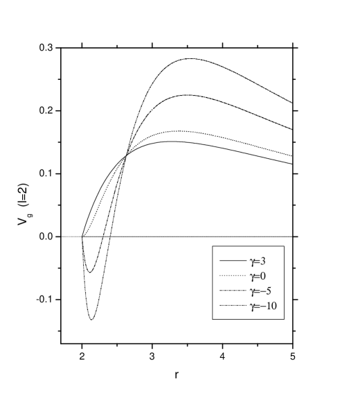
Figure 4: The effective potentials of the gravitational perturbation for different $\gamma$ and $l$.

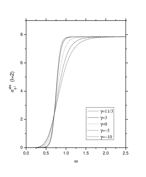
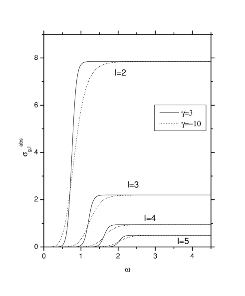
Figure 5: Partial energy absorption of the gravitational wave for different $\gamma,l$.

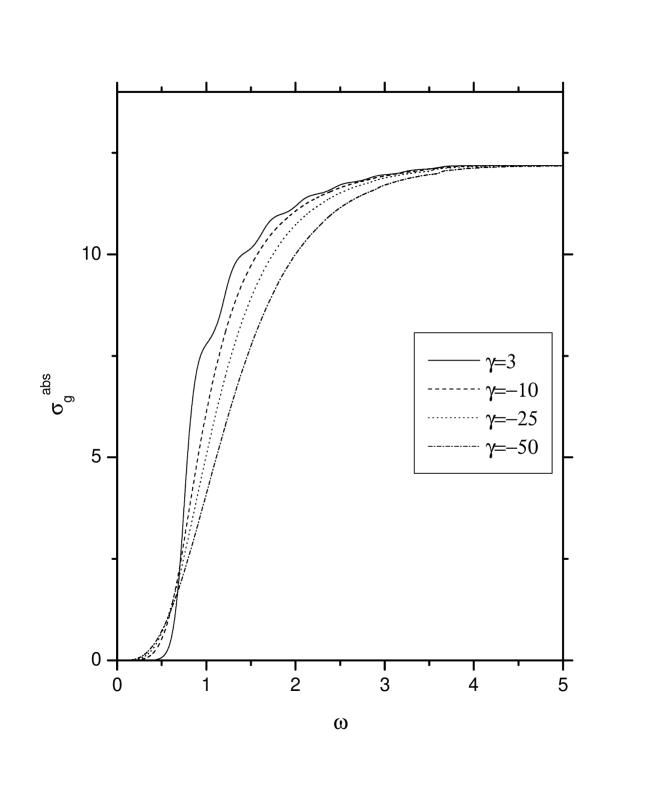
Figure 6: Total energy absorption of the gravitational wave.

In solving the radial equation Eq. (60), we choose a particular solution $\phi_{l}(r)$ to be normalized as

$$\phi_{l}(r)=p_{l}^{-1}Z_{l}(r).$$ (162)

In the remote region, it consists of the outgoing and ingoing waves, which is

$$\phi_{l}(r)=n_{l}^{(-)}\mathcal{N}_{l(+)}+n_{l}^{(+)}\mathcal{N}_{l(-)},$$ (163)

where

$$\mathcal{N}_{l(\pm)}(r)=e^{\mp i\omega r_{*}}\sum_{n=0}^{\infty}\kappa^{(\pm)}_{l,n}\left(\frac{r_{H}}{r}\right)^{n},$$ (164)

and the combination coefficients $n_{l}^{(\pm)}$ are called jost functions. To obtain the jost functions numerically, we calculate their Wronskian, by applying Eq. (144) we arrive at

$$W[\mathcal{N}_{l(+)},\mathcal{N}_{l(-)}]=\frac{2i\omega}{\sqrt{AB}}.$$ (165)

The jost functions read

$$n_{l}^{(\pm)}=\mp\frac{\sqrt{AB}}{2i\omega}W[\phi_{l},\mathcal{N}_{l(\pm)}].$$ (166)

Comparing Eq. (163) with Eq. (71), we have

$$p_{l}=(-1)^{l}\frac{(2l+1)\omega}{12\ n_{l}^{(-)}},$$ (167)

$$S_{l}^{g}=(-1)^{l+1}\frac{n_{l}^{(+)}}{n_{l}^{(-)}}.\ \ \$$ (168)

They are key quantities for determining the absorption cross section.

In practice, we insert Eq. (167) into Eq. (142) and Eq. (143), and have

$$\sigma_{g,l}^{abs}=12\pi r_{H}^{2}\frac{(l-2)!}{(l+2)!}\frac{2l+1}{|n_{l}^{(-)}|^{2}},$$ (169)

and

$$\sigma_{g}^{abs}=12\pi r_{H}^{2}\sum_{l=2}^{\infty}\frac{(l-2)!}{(l+2)!}\frac{2l+1}{|n_{l}^{(-)}|^{2}}.$$ (170)

Now we can do the numerical calculation. Substituting the CFM black hole metric, for the gravitational perturbation, the effective potential has the form

$$V_{g,l}(r)=\left(1-\frac{2M}{r}\right)\left[\frac{l(l+1)}{r^{2}}-\frac{6M}{r^{3}}-\frac{M(\gamma-3)(5r^{2}-20Mr+18M^{2})}{r^{3}(2r-3M)^{2}}\right].$$ (171)

Choosing $M=1$, we display the behavior of the potential for the axial perturbation in Fig.4. The effective potential is not positive definite. For enough negative value of $\gamma$, a negative peak will show up out of the horizon. The negative potential well becomes deeper when $\gamma$ becomes more negative for fixed $l$. For chosen $\gamma$, the negative potential well appears for small $l$. Compared with the scalar case, in the gravitational perturbation, the negative wells appear before the potential barriers. It was argued that negative potential may result in the amplification of the perturbation out of the black hole and cause the spacetime to be unstable wang01 . However in the QNM study of the CFM braneworld black hole eabdalla , it was shown that even for very negative value of $\gamma$, the perturbative dynamics out of the black hole is always stable. The negative potential well loses the competition with the positive potential barrier and the perturbative dynamics is still dominated by the positive potential barrier.

In the study of the absorption, the potential well tends to enhance the absorption while the barrier tends to decrease it. The result on the partial absorption cross section is shown in Fig.5. We find that as the case observed in the QNM study eabdalla , the potential barrier wins the competition with the well and dominates the contribution to the absorption rate. Fixing $l$, we observe that for more negative $\gamma$, less gravitational wave energy is absorbed by the CFM braneworld black hole. And for chosen $\gamma$, the absorption rate decreases with the increase of $l$ due to higher potential barrier. In the low $\omega$ region, the absorption is enhanced for smaller values of $\gamma$, which is the effect of the negative potential well.

In the high energy limit, the partial absorption cross sections of the gravitational wave flatten out which is different from the case in the scalar wave. This is due to the difference in Eq. (38) and Eq. (149), where in the scalar case the partial section is proportional to $\omega^{-2}$ in the high frequency regime, while in the gravitational wave case, the partial section is proportional to $\omega^{0}$ in the high frequency regime. Deep reason causing this difference lies in the different expansions of the plane wave. In the scalar case, the plane wave is expanded in terms of Legendre polynomials into spherical waves with a factor $(\omega r)^{-1}e^{\pm i\omega r}$ (Eq. [12]), while in the gravitational case, it is expanded in Gegenbauer polynomials into the wave with a factor $(\omega r)e^{\pm i\omega r}$ (Eq. [III.2.1]).

The result on the total absorption cross section of the gravitational wave is shown in Fig.6. The total absorption cross section, which is the physically observable quantity, behaves in a similar manner to that in the scalar case. This shows that the difference in the gravitational partial absorption cross section from that of the scalar case is more mathematical than physical.

IV Conclusion and Discussion

In this paper, we have studied the energy absorption problem of the scalar wave as well as the axial gravitational wave in the background of the CFM brane-world black hole. The CFM black hole is spherical and has only one event horizon at $r_{H}=2M$. When the parameter $\gamma=3$, the CFM braneworld black hole returns to the Schwarzschild solution. In comparison with Schwarzschild black hole, the CFM braneworld black hole will be either hotter or colder depending upon whether $\gamma<3$ or $\gamma>3$.

We have calculated the scalar perturbation and the axial gravitational perturbation around the brane black hole and evaluated the energy absorptions of the scalar and gravitational waves. Comparing with the 4D Schwarzschild black hole when $\gamma=3$, we observed that the energy absorption of the braneworld black hole decreases with the decrease of $\gamma$ starting from 3. While when $\gamma>3$ we found that the energy absorption enhanced compared with that of the Schwarzschild black hole. We restricted to the case $\gamma\leq 11/3$. This result holds the same for both the scalar wave and axial gravitational wave outside the CFM hole. In both perturbations, the negative potential well appeared, however the positive potential barrier still dominated in determining the absorption rate, which has the same effect as observed in the QNM study. The result on the absorption spectrum implies that for $\gamma<3$, the black hole emission will be enhanced with the decrease of $\gamma$, while for $\gamma>3$, the emission of the black hole will be suppressed, which is consistent with the behavior of the Hawking temperature of the braneworld black hole. We conclude that the energy absorption for the scalar and axial gravitational wave gives signatures of the bulk effects in the brane-world black hole, which differs from that of the 4D Schwarzschild black hole. We expect that these signatures can be observed in the future experiments, which could help us learn the properties of the extra dimensions.

In the study of the axial gravitation perturbation, the deduction of $\Psi_{0}^{(1)}=\tilde{\Psi}_{0}^{(1)}$ helps us a lot in doing the calculation, however the simplification is obviously not hold for polar perturbation. Thus it is of interest to generalize our discussion in the future to study on the polar gravitation wave.

It needs to be emphasized that although several spherically symmetric and static brane black hole solutions with contributions from the bulk gravity have been found, none of these are obtained as exact solutions of the full five-dimensional bulk field equations s14 . The propagation of gravity into the bulk does not permit the treatment of the brane gravitational field equations as a closed system. This fact limits the consideration of propagating modes of fields off the brane. Although the propagating modes in the bulk are hard to be obtained at the present moment, the modes on the brane are still interesting since they are the most phenomenologically interesting effects which can be detected during experiments. Furthermore, it was argued that the emission of particle modes on the brane is dominant compared to that off the brane s10 . Brane localized modes have been investigated to disclose the information of extra-dimensions in different attempts eabdalla ; shen ; s11 ; s12 ; park ; park2 . Despite that we cannot obtain the propagating modes in the bulk due to the lack of complete bulk solutions owing to the conceptually complicated gravitational field equations, our study of brane modes is still well-motivated and interesting. Employing the Newman-Penrose formalism, we have provided a test of the energy absorption spectrum of a new braneworld black hole solution.

- (1) N. Arkani-Hamed, S. Dimopoulos and G. Dvali, Phys. Lett. B 429, 263 (1998); I. Antoniadis, N. Arkani-Hamed, S. Dimopoulos, G.R. Dvali, Phys. Lett. B436, 257 (1998)
- (2) L. Randall and R. Sundrum, Phys. Rev. Lett. 83, 3370 (1999); Phys. Rev. Lett. 83, 4690 (1999).
- (3) K. Akama, Lect.Notes Phys. 176, 267 (1982); V.A. Rubakov and M.E. Shaposhnikov, Phys. Lett. B125, 139 (1983); M. Visser, Phys. Lett. B159, 22 (1985); M. Gogberashvili, Europhys. Lett. 49, 396 (2000).
- (4) T. Banks and W. Fischler, hep-th/9906038.
- (5) S. B. Giddings and S. Thomas, Phys. Rev. D65, 056010 (2002).
- (6) S. Dimopoulos and G. Landsberg, Phys. Rev. Lett. 87, 161602 (2001).
- (7) C. M. Harris, P. Kanti, JHEP 0310, 014 (2003).
- (8) H. P. Nollert, Class. Quant. Grav. 16, R159 (1999); K. D. Kokkotas and B. G. Schmidt, Living Rev. Rel. 2, 2 (1999); B. Wang, Braz. J. Phys. 35, 1029 (2005).
- (9) P. Kanti, R. A. Konoplya, A. Zhidenko, gr-qc/0607048 ; P. Kanti, R.A. Konoplya, Phys. Rev. D73, 044002 (2006); D. K. Park, Phys. Lett. B633, 613 (2006).
- (10) E. Abdalla, B. Cuadros-Melgar, A. B. Pavan and C. Molina, gr-qc/0604033, Nuclear Phys. B 752 (2006) 40-59;
- (11) Jianyong Shen, Bin Wang, Ru-Keng Su, Phys.Rev. D74 (2006) 044036.
- (12) P. Kanti, hep-ph/0310162.
- (13) C. M. Harris and P. Kanti, JHEP 0310 014 (2003) ; P. Kanti, Int. J. Mod. Phys. A19 4899 (2004); P. Argyres, S. Dimopoulos and J. March-Russell, Phys. Lett. B441 96 (1998); T. Banks and W. Fischler, hep-th/9906038; R. Emparan, G. T. Horowitz and R. C. Myers, Phys. Rev. Lett. 85 499 (2000).
- (14) E. Jung and D. K. Park, Nucl. Phys. B717 272 (2005); N. Sanchez, Phys. Rev. D18 1030 (1978); E. Jung and D. K. Park, Class. Quant. Grav. 21 3717 (2004).
- (15) A. S. Majumdar, N. Mukherjee, Int.J.Mod.Phys. D14 1095 (2005) and reference therein; G. Kofinas, E. Papantonopoulos and V. Zamarias, Phys.Rev. D66, 104028 (2002); G. Kofinas, E. Papantonopoulos and V. Zamarias, Astrophys.Space Sci. 283, 685 (2003); A. N. Aliev, A. E. Gumrukcuoglu, Phys. Rev. D71, 104027 (2005); S. Kar, S. Majumdar, hep-th/0510043; S. Kar, S. Majumdar, hep-th/0606026; S. Kar, hep-th/0607029.
- (16) C. M. Harris and P. Kanti, JHEP 0310 (2003) 014; E. Jung and D. K. Park, Nucl. Phys. B717 (2005) 272; V. Frolov and D. Stojkovi¡äc, Phys. Rev. D67 (2003) 084004.
- (17) E. Jung, S. H. Kim and D. K. Park, Phys. Lett. B615 273 (2005); E. Jung, S. H. Kim and D. K. Park, Phys. Lett. B619 347 (2005); D. Ida, K. Oda and S. C. Park, Phys. Rev. D67 064025 (2003); C. M. Harris and P. Kanti, Phys.Lett. B633 106 (2006); D. Ida, K. Oda and S. C. Park, Phys. Rev. D71 124039 (2005); G. Duffy, C. Harris, P. Kanti and E. Winstanley, JHEP 0509 049 (2005); M. Casals, P. Kanti and E. Winstanley, JHEP 0602 051 (2006); E. Jung and D. K. Park, Nucl. Phys. B731 171 (2005); A. S. Cornell, W. Naylor and M. Sasaki, JHEP 0602, 012 (2006); V. P. Frolov, D. Stojkovic, Phys. Rev. Lett. 89, 151302 (2002); Valeri P. Frolov, Dejan Stojkovic, Phys. Rev. D66, 084002 (2002); D. Stojkovic, Phys. Rev. Lett. 94, 011603 (2005).
- (18) D.K. Park, hep-th/0512021
- (19) Eylee Jung and D. K. Park, hep-th/0612043; V. Cardoso, M. Cavaglia, L. Gualtieri, Phys. Rev. Lett. 96, 071301 (2006); V. Cardoso, M. Cavaglia, L. Gualtieri, JHEP 0602, 021 (2006).
- (20) D. Dai, N. Kaloper, G. Starkman and D. Stojkovic, hep-th/0611184.
- (21) R. Emparan, G. T. Horowitz and R. C. Myers, Phys. Rev. Lett. 85 (2000) 499.
- (22) N. Kaloper and D. Kiley, JHEP 0603, 077 (2006)
- (23) R. Casadio, A. Fabbri and L. Mazzacurati, Phys. Rev. D 65, 084040 (2002).
- (24) R. Casadio, L. Mazzacurati, Mod.Phys.Lett. A18 (2003) 651.
- (25) S. Chandrasekhar, The Mathematical Theory of Black Holes, (Oxford, New York, 1983)
- (26) N. G. Sánchez, Phys. Rev. D16, 937 (1977); N. G. Sánchez, J. Math. Phys., 17, 688 (1976); N. G. Sánchez, Phys. Rev. D18, 1030 (1978)
- (27) S. Persides, J. Math. Phys., 14, 1017 (1973).
- (28) S. A. Teukolsky Ap. J., 185, 635 (1973); S. A. Teukolsky, W. H. Press, Ap. J., 194, 443 (1974)
- (29) T. Shiromizu, K. Maeda, M. Sasake, Phys. Rev., D62, 024012 (2000)
- (30) Elcio Abdalla, Bertha Cuadros-Melgar, Sze-Shiang Feng, Bin Wang, Phys.Rev. D65, 083512 (2002); Elcio Abdalla, Adenauer G. Casali, Bertha Cuadros-Melgar, Int. J. Theor. Phys. 43, 801 (2004); Nucl. Phys. B644, 201 (2002).
- (31) I. S. Gradshteyn, I. M. Ryzhik, Tables of Integrals, Series and Products (Academic, New York, 1965)
- (32) W. Kinnersley, J. Math. Phys., 25, 152 (1969)
- (33) S. W. Hawking, J. B. Hartle, Comm. Math. Phys., 27, 283 (1972)
- (34) R. A. Isaacson, Phys. Rev., 166, 1272 (1968)
- (35) Bin Wang, Elcio Abdalla, R. B. Mann, Phys.Rev. D65 (2002) 084006