Topics in Cosmology

Abstract:

These lectures present a brief review of inflationary cosmology, provide an overview of the theory of cosmological perturbations, and then focus on the conceptual problems of the current paradigm of early universe cosmology, thus motivating an exploration of the potential of string theory to provide a new paradigm. Specifically, the string gas cosmology model is introduced, and a resulting mechanism for structure formation which does not require a period of cosmological inflation is discussed.

1 Introduction and Overview

These lectures focus on three topics. The first is an overview of the current paradigm of early universe cosmology, the inflationary universe scenario. The second topic is a pedagogical presentation of the theory of cosmological perturbations, the main tool of modern cosmology which allows us to connect theories of the very early universe with observational data. The third topic is string gas cosmology, an attempt to construct a new scenario of the very early universe based on established principles of string theory.

Over the past two and a half decades, cosmology has become a science dominated by data of rapidly increasing accuracy. Today, we have three-dimensional maps of the distribution of galaxies in space which contain more than one hundred thousand galaxies [2, 3]. They clearly indicate that luminous matter in the universe is neither uniformly nor randomly distributed. There are clear patterns to be seen: clusters of galaxies, superclusters, filaments and voids (regions of space empty of galaxies). The distribution can be quantified in terms of the luminosity power spectrum. A key challenge for cosmology is to understand the origin of these patterns in the distribution of matter.

Another observational window in cosmology is the cosmic microwave background (CMB) radiation. Overall, this radiation is characterized by a surprising isotropy. At a fractional level of a bit less than $10^{-4}$, however, there are anisotropies. These can be quantified in terms of their angular power spectrum. First, the sky map (two-dimensional) of anisotropies is expanded in spherical harmonics $Y_{lm}$:

$${{\Delta T}\over T}(\theta,\varphi)\,=\,\sum_{l=1}^{\infty}\sum_{m=-l}^{l}a_{lm}Y_{lm}(\theta,\varphi)$$ (1)

where $\theta$ and $\phi$ are the usual angles on the surface of the sphere. If the fluctuations are due to a Gaussian random process with no distinguished direction in the sky, then the complete information about the fluctuations is given by the ensemble average (denoted by pointed parentheses) of the coefficients $a_{lm}$:

$$c_{l}\,=\,<|a_{lm}|^{2}>\,,$$ (2)

These $c_{l}$ coefficients define the angular power spectrum of CMB anisotropies. Figure 1 is the full sky map of CMB anisotropies from the WMAP experiment [4]. Figure 2 shows the resulting angular power spectrum )(what is plotted on the vertical axis is $l(l+1)C_{l}/(2\pi)$). The key features are the flat region at small values of $l$ (large angular scales) and the characteristic oscillations of the spectrum at intermediate angular scales. Another crucial challenge for cosmology is to explain both the overall isotropy of the CMB, and the specific patterns of anisotropies.

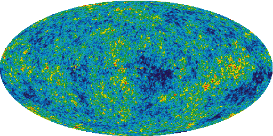
Figure 1: All sky map of the temperature anisotropies in the CMB from the WMAP satellite experiment. Credit: NASA/WMAP Science Team.

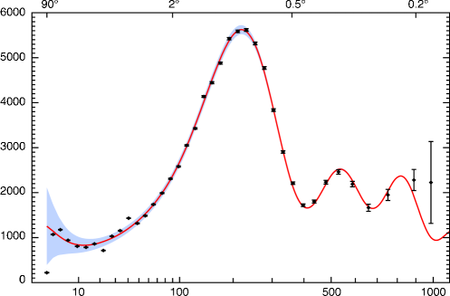
Figure 2: The power spectrum of CMB anisotropies as computed from the WMAP satellite experiment. The horizontal axis is the angular quantum number $l$, the vertical axis gives the power of the CMB on the respective scales. The dots represent the data points (with their errors bars indicated), the solid curve is the prediction of the best-fit inflationary model. Credit: NASA/WMAP Science Team.

According to our present understanding, we must look to the very early universe to find an explanation for the observed structures. The reason is that in Standard Big Bang cosmology (SBB), which well describes the cosmological evolution at late times (times later and including the period of nucleosynthesis) the physical wavelength of fixed comoving scales is increasing less fast than the Hubble radius (an important length scale which is defined and whose role is described at the end of this section). Hence, the scales which are currently observed were outside of the Hubble radius at early times, and no causal structure formation scenario is possible .

It is a remarkable success of inflationary cosmology, our current paradigm of early universe cosmology, that it, in addition to explaining why the universe is large, spatially flat, and containing a large amount of entropy, provides a causal mechanism for the origin of inhomogeneities in the universe. The solid curve in Figure 2 represents the predictions of inflationary cosmology The predictions were made more than 15 years before the data shown in Figure 1 were collected.

In these lectures, however, I would like to focus less on the phenomenological successes of the inflationary paradigm, but more on the conceptual problems which current realizations of inflationary cosmology are confronted with. These problems call out for the development of a new paradigm, a paradigm which must include new fundamental physics, a theory which better describes space, time and matter and the highest densities. The best current candidate for such a theory is superstring theory. Hence, in the third main part of these lectures (Section 4) I will explore the possibility that string theory may lead to a new paradigm of early universe cosmology. My approach to string cosmology in this section is complementary to the one taken in the lectures of Cliff Burgess at this school (see [8]), in which avenues of obtaining inflation in the context of models coming from string theory are explored (see also [9, 10] for other reviews of such avenues).

The theory of cosmological perturbations plays a key role in modern cosmology, since it provides the techniques with which to calculate, in the context of any given scenario of the very early universe, the generation and evolution of the predicted inhomogeneities in the matter distribution and anisotropies in the CMB, and thus allows for a comparison between fundamental theory and observational data. The second part of these lectures (Section 3) provides a pedagogical overview of this theory.

I begin, however, with a discussion of inflationary cosmology, the current paradigm of cosmology.

To establish our notation and framework, we will be taking the background space-time to be homogeneous and isotropic, with a metric given by

$$ds^{2}\,=\,dt^{2}-a(t)^{2}d{\bf x}^{2}\,,$$ (3)

where $t$ is physical time, $d{\bf x}^{2}$ is the Euclidean metric of the spatial hypersurfaces (here taken for simplicity to be spatially flat), and $a(t)$ is the scale factor. The scale factor determines the Hubble expansion rate via

$$H(t)\,=\,{{\dot{a}}\over a}(t)\,.$$ (4)

The coordinates ${\bf x}$ used above are comoving coordinates, coordinates painted onto the expanding spatial hypersurfaces.

We are interested in tracking the time evolution of the physical wavelength of the currently observed patterns in the distribution of matter and of the CMB anisotropies. Since the patterns are assumed to be frozen in in comoving coordinates, the physical wavelength scales as $a(t)$.

A key length scale in cosmology is the Hubble radius

$$l_{H}(t)\,=\,H^{-1}(t)\,,$$ (5)

defined to be the inverse Hubble expansion rate. As will be explained later, the Hubble radius is the maximal distance that microphysics can act coherently over a Hubble expansion time - in particular it is the maximal distance on which any causal process could create fluctuations.

2 Inflationary Cosmology: The Current Paradigm

Standard Big Bang (SBB) cosmology, the precursor to inflationary cosmology as the paradigm for the evolution of the early universe, is based on a classical physics description of both space-time (via Einstein’s theory of General Relativity) and matter (a superposition of two perfect fluids, the first describing pressureless matter - cold matter - the second describing radiation - the CMB). The key phenomenological success of the SBB model is the prediction of the existence and black body nature of the CMB, the black body nature of which was confirmed with spectacular accuracy by the COBE satellite [11] and UBC rocket experiments [12].

On the other hand, the SBB scenario leaves many crucial questions un-answered [13]. Why is the universe so close to spatially flat? Why is it so large and contains such a large entropy? Why is the CMB isotropic to an accuracy of better than $10^{-4}$ (after subtracting the dipole contributions due to our motion relative to the rest frame of the CMB and the effects due to the emission of our own galaxy)? Most importantly, what is the origin of the observed inhomogeneities in the distribution of matter and of the small CMB anisotropies? These are the “flatness”, “entropy”, “horizon” and “structure formation” problems of SBB cosmology. SBB also suffers from conceptual problems: the initial cosmological singularity tells us both that the theory must be incomplete, and that it is based on using the wrong fundamental physics input close to the singularity .

Inflationary cosmology [13] (see also [14, 15, 16]) provides an solution of the horizon, flatness and entropy problems. In addition, it provides a mechanism for the origin of structure in the universe based on causal physics [17] (see also [18, 14]).

The idea of inflationary cosmology is to assume that there was a period in the very early Universe during which the scale factor was accelerating, i.e. ${\ddot{a}}>0$. This implies that the Hubble radius was shrinking in comoving coordinates, or, equivalently, that fixed comoving scales were “exiting” the Hubble radius. In the simplest models of inflation, the scale factor increases nearly exponentially.

Figure 3: Space-time diagram (sketch) showing the evolution of scales in inflationary cosmology. The vertical axis is time, and the period of inflation lasts between $t_{i}$ and $t_{R}$, and is followed by the radiation-dominated phase of standard big bang cosmology. During exponential inflation, the Hubble radius $H^{-1}$ is constant in physical spatial coordinates (the horizontal axis), whereas it increases linearly in time after $t_{R}$. The physical length corresponding to a fixed comoving length scale labelled by its wavenumber $k$ increases exponentially during inflation but increases less fast than the Hubble radius (namely as $t^{1/2}$), after inflation.

As illustrated in Figure 3, the basic geometry of inflationary cosmology provides a solution of the fluctuation problem. As long as the phase of inflation is sufficiently long, all length scales within our present Hubble radius today originate at the beginning of inflation with a wavelength smaller than the Hubble radius at that time. Thus, it is possible to create perturbations locally using physics obeying the laws of special relativity (in particular causality). As will be discussed later, it is quantum vacuum fluctuations of matter fields and their associated curvature perturbations which are predicted to be responsible for the structure we observe today.

Postulating a phase of inflation in the very early universe solves the horizon problem of the SBB, namely it explains how the causal horizon at the time $t_{rec}$ when photons last scatter can be larger than the radius of the past light cone at $t_{rec}$, the part of the last scattering surface which is visible today in CMB experiments. Inflation explains the near flatness of the universe: in a decelerating universe spatial flatness is an unstable fixed point of the dynamics, whereas in an accelerating universe it becomes an attractor. Another important feature of inflation is that the volume of space increases exponentially at constant energy density. If this energy density is successfully converted to ordinary matter at the end of the period of inflation, then the entropy of the universe is exponentially larger after compared to before inflation. In addition, with the exponential expansion of space it is easy to produce a universe of our size today from a Planck scale universe at the initial Planck time, something which is not possible in the SBB model. Thus inflation explains the large current size and entropy of the universe.

Let us now consider how it is possible to obtain a phase of cosmological inflation. We will assume that space-time is described using the equations of General Relativity . In this case, the dynamics of the scale factor $a(t)$ is determined by the Friedmann-Robertson-Walker (FRW) equations

$$({{\dot{a}}\over a})^{2}\,=\,8\pi G\rho$$ (6)

and

$${{\ddot{a}}\over a}\,=\,-4\pi G(\rho+3p)$$ (7)

where for simplicity we have omitted the contributions of spatial curvature (since spatial curvature is diluted during inflation) and of the cosmological constant (since any small cosmological constant which might be present today has no effect in the early Universe since the associated energy density does not increase when going into the past). In the above, $\rho$ and $p$ denote the energy density and pressure, respectively. From (7) it is clear that in order to obtain an accelerating universe, matter with sufficiently negative pressure

$$p\,<\,-{1\over 3}\rho$$ (8)

is required. Exponential inflation is obtained for $p=-\rho$.

Conventional perfect fluids have positive semi-definite pressure and thus cannot yield inflation. However, we know that a description of matter in terms of classical perfect fluids must break down at early times. An improved description of matter will be given in terms of quantum fields. Scalar matter fields are special in that they allow at the level of a renormalizable action the presence of a potential energy term. The energy density and pressure of a scalar field $\varphi$ with canonically normalized action

$$S\,=\,\int d^{4}x\sqrt{-g}\bigl{[}{1\over 2}\partial_{\mu}\varphi\partial^{\mu}\varphi-V(\varphi)\bigr{]}\,$$ (9)

(where Greek indices label space-time coordinates, $V(\varphi)$ is the potential energy density, and $g$ is the determinant of the metric) are given by

$$\rho\, = \,{1\over 2}({\dot{\varphi}})^{2}+{1\over 2}a^{-2}(\nabla\varphi)^{2}+V(\varphi)$$

$$p\, = \,{1\over 2}({\dot{\varphi}})^{2}-{1\over 6}a^{-2}(\nabla\varphi)^{2}-V(\varphi)\,.$$ (10)

Thus, it is possible to obtain an almost exponentially expanding universe provided the scalar field configuration satisfies

$${1\over 2}(\nabla_{p}\varphi)^{2}\, \ll \,V(\varphi)\,,$$ (11)

$${1\over 2}({\dot{\varphi}})^{2}\, \ll \,V(\varphi)\,.$$ (12)

In the above, $\nabla_{p}\equiv a^{-1}\nabla$ is the gradient with respect to physical as opposed to comoving coordinates. Since spatial gradients redshift as the universe expands, the first condition will (for single scalar field models) always be satisfied if it is satisfied at the initial time . It is the second condition which is harder to satisfy. In particular, this condition is in general not preserved in time even it is initially satisfied [21].

It is sufficient to obtain a period of cosmological inflation that the slow-roll conditions for $\varphi$ are satisfied. Recall that the equation of motion for a homogeneous scalar field in a cosmological space-time is (as follows from (9)) is

$${\ddot{\varphi}}+3H{\dot{\varphi}}\,=\,-V^{\prime}(\varphi)\,,$$ (13)

where a prime indicates the derivative with respect to $\varphi$. In order that the scalar field roll slowly, it is necessary that

$${\ddot{\varphi}}\,\ll\,3H{\dot{\varphi}}$$ (14)

such that the first term in the scalar field equation of motion (13) is negligible. In this case, the condition (12) becomes

$$({{V^{\prime}}\over V})^{2}\,\ll\,48\pi G\,$$ (15)

and (14) becomes

$${{V^{\prime\prime}}\over V}\,\ll\,24\pi G\,.$$ (16)

In the initial model of inflation using scalar fields (“old inflation” [13]), it was assumed that $\varphi$ was initially in a false vacuum with large potential energy. Hence, the conditions for inflation are trivially satisfied. To end inflation, a quantum tunneling event from the false vacuum to the true vacuum [22] was invoked (see e.g. [23] for a pedagogical review). This model, however, has a graceful exit problem since the tunneling leads to an initially microscopical bubble of the true vacuum which cannot grow to encompass our presently observed universe - the flatness problem of SBB cosmology in a new form. Hence, attention shifted to models in which the scalar field $\varphi$ is slowly rolling during inflation.

There are many models of scalar field-driven inflation. Many of them can be divided into three groups [24]: small-field inflation, large-field inflation and hybrid inflation. Small-field inflationary models are based on ideas from spontaneous symmetry breaking in particle physics. We take the scalar field to have a potential of the form

$$V(\varphi)\,=\,{1\over 4}\lambda(\varphi^{2}-\sigma^{2})^{2}\,,$$ (17)

where $\sigma$ can be interpreted as a symmetry breaking scale, and $\lambda$ is a dimensionless coupling constant. The hope of initial small-field models (“new inflation” [25]) was that the scalar field would begin rolling close to its symmetric point $\varphi=0$, where thermal equilibrium initial conditions would localize it in the early universe. At sufficiently high temperatures, $\varphi=0$ is a stable ground state of the one-loop finite temperature effective potential $V_{T}(\varphi)$ (see e.g. [23] for a review). Once the temperature drops to a value smaller than the critical temperature $T_{c}$, $\varphi=0$ turns into an unstable local maximum of $V_{T}(\varphi)$, and $\varphi$ is free to roll towards a ground state of the zero temperature potential (17). The direction of the initial rolling is triggered by quantum fluctuations. The reader can easily check that for the potential (17) the slow-roll conditions cannot be satisfied if $\sigma\ll m_{pl}$, where $m_{pl}$ is the Planck mass which is related to $G$. If the potential is modified to a Coleman-Weinberg [26] form

$$V(\varphi)\,=\,{{\lambda}\over 4}\varphi^{4}\bigl{[}{\rm ln}{{|\varphi|}\over{\sigma}}-{1\over 4}\bigr{]}+{1\over{16}}\lambda\sigma^{4}$$ (18)

(where $\sigma$ denotes the value of the minimum of the potential) then the slow-roll conditions can be satisfied. However, this corresponds to a severe fine-tuning of the shape of the potential. A further problem for most small-field models of inflation (see e.g. [21] for a review) is that the slow-roll trajectory is not an attractor in phase space. In order to end up close to the slow-roll trajectory, the initial field velocity must be constrained to be very small. This initial condition problem of small-field models of inflation effects a number of recently proposed brane inflation scenarios, see e.g. [27] for a discussion.

There is another reason for abandoning small-field inflation models: in order to obtain a sufficiently small amplitude of density fluctuations, the interaction coefficients of $\varphi$ must be very small (this problem is discussed in detail at the beginning of Section 4). In particular, this makes it inconsistent to assume that $\varphi$ started out in thermal equilibrium. In the absence of thermal equilibrium, the phase space of initial conditions is much larger for large values of $\varphi$.

This brings us to the discussion of large-field inflation models, initially proposed in [28] under the name “chaotic inflation”. The simplest example is provided by a massive scalar field with potential

$$V(\varphi)\,=\,{1\over 2}m^{2}\varphi^{2}\,,$$ (19)

where $m$ is the mass. It is assumed that the scalar field rolls towards the origin from large values of $|\varphi|$. It is a simple exercise for the reader to verify that the slow-roll conditions (15) and (16) are satisfied provided

$$|\varphi|\,>\,{1\over{\sqrt{12\pi}}}m_{pl}\,.$$ (20)

Values of $|\varphi|$ comparable or greater than $m_{pl}$ are also required in other realizations of large-field inflation. Hence, one may worry whether such a toy model can consistently be embedded in a realistic particle physics model, e.g. supergravity. In many such models $V(\varphi)$ receives supergravity-induced correction terms which destroy the flatness of the potential for $|\varphi|>m_{pl}$. However, as discussed e.g. in [29], if the flatness of the potential is protected by some symmetry, then it can survive inclusion of the correction terms. As will be discussed later, a value of $m\sim 10^{13}$GeV is required in order to obtain the observed amplitude of density fluctuations. Hence, the configuration space of field values with $|\varphi|>m_{pl}$ but $V(\varphi)<m_{pl}^{4}$ is huge. It can also be verified that the slow-roll trajectory is a local attractor in field initial condition space [20], even including metric fluctuations at the perturbative level [30].

With two scalar fields it is possible to construct a class of models which combine some of the nice features of large-field inflation (large phase space of initial conditions yielding inflation) and of small-field inflation (inflation taking place at sub-Planckian field values). These are models of hybrid inflation [31]. To give a prototypical example, consider two scalar fields $\varphi$ and $\chi$ with a potential

$$V(\varphi,\chi)\,=\,{1\over 4}\lambda_{\chi}(\chi^{2}-\sigma^{2})^{2}+{1\over 2}m^{2}\varphi^{2}-{1\over 2}g^{2}\varphi^{2}\chi^{2}\,.$$ (21)

In the absence of thermal equilibrium, it is natural to assume that $|\varphi|$ begins at large values, values for which the effective mass of $\chi$ is positive and hence $\chi$ begins at $\chi=0$. The parameters in the potential (21) are now chosen such that $\varphi$ is slowly rolling for values of $|\varphi|$ somewhat smaller than $m_{pl}$, but that the potential energy for these field values is dominated by the first term on the right-hand side of (21). The reader can easily verify that for this model it is no longer required to have values of $|\varphi|$ greater than $m_{pl}$ in order to obtain slow-rolling The field $\varphi$ is slowly rolling whereas the potential energy is determined by the contribution from $\chi$. Once $|\varphi|$ drops to the value

$$|\varphi_{c}|\,=\,{{{\sqrt{\lambda_{\chi}}}}\over g}\sigma$$ (22)

the configuration $\chi=0$ becomes unstable and decays to its ground state $|\chi|=\sigma$, yielding a graceful exit from inflation. Since in this example the ground state of $\chi$ is not unique, there is the possibility of the formation of topological defects at the end of inflation (see [5, 6, 7] for reviews of topological defects in cosmology, and the lectures by Polchinski [32] for a discussion of how this scenario arises in brane inflation models).

After the slow-roll conditions break down, the period of inflation ends, and the inflaton begins to oscillate around its ground state. Due to couplings of $\varphi$ to other matter fields, the energy of the universe, which at the end of the period of inflation is stored completely in $\varphi$, gets transferred to the matter fields of the particle physics Standard Model. Initially, the energy transfer was described perturbatively [33, 34]. Later, it was realized [35, 36, 37, 38] that through a parametric resonance instability, particles are very rapidly produced, leading to a fast energy transfer (“preheating”). The quanta later thermalize, and thereafter the universe evolves as described by SBB cosmology.

3 Theory of Cosmological Perturbations: A Short Review

After this review of inflationary cosmology (see e.g. [39] for a more complete recent review), we turn to the discussion of the main success of inflationary cosmology, namely the fact that it provides a causal mechanism for generating small amplitude inhomogeneities. The reader is referred to [40] for a comprehensive analysis of this theory of cosmological perturbations, and [41] for a pedagogical overview, from which most of this section is drawn.

First, we describe the Newtonian theory of cosmological perturbations, mainly to develop intuition for the main physical effects. The range of validity of the Newtonian analysis is restricted to sub-Hubble scales at late times. In the second subsection, we then summarize the general relativistic theory of fluctuations. Linear fluctuations can be trivially quantized. The quantization of cosmological perturbations is presented in Subsection 3.

3.1 Newtonian Theory of Cosmological Perturbations

The growth of density fluctuations is a consequence of the purely attractive nature of the gravitational force. Given an density excess $\delta\rho$ localized about some point ${\bf x}$ in space. This inhomogeneity produces a force which attracts the surrounding matter towards ${\bf x}$. The magnitude of this force is proportional to $\delta\rho$. Hence, in a non-expanding background, by Newton’s second law

$$\ddot{\delta\rho}\,\sim\,G\delta\rho\,,$$ (23)

where $G$ is Newton’s gravitational constant. Thus, an exponential growth of the fluctuations is induced.

If, as required by consistency in General Relativity, we consider density fluctuations in an expanding background, then the expansion of space leads to a friction term in (23). Hence, instead of an exponential instability to the development of fluctuations, the growth of fluctuations will be as a power of time. The main goal of the theory of cosmological perturbations is to determine how the power-law instability depends on the background cosmology and on the length scale of the fluctuations.

3.2 Perturbations about Minkowski Space-Time

To develop some physical intuition, we first consider the evolution of hydrodynamical matter fluctuations in a fixed non-expanding background.

In this context, matter is described by a perfect fluid, and gravity by the Newtonian gravitational potential $\varphi$. The fluid variables are the energy density $\rho$, the pressure $p$, the fluid velocity ${\bf v}$, and the entropy density $S$. The basic hydrodynamical equations are

$$\dot{\rho}+\nabla_{p}\cdot(\rho{\bf v}) = 0$$

$$\dot{{\bf v}}+({\bf v}\cdot\nabla_{p}){\bf v}+{1\over{\rho}}\nabla_{p}p+\nabla_{p}\varphi = 0$$

$$\nabla_{p}^{2}\varphi = 4\pi G\rho$$ (24)

$$\dot{S}+({\bf v}\cdot\nabla_{p})S = 0$$

$$p = p(\rho,S)\,,$$

where the subscript $p$ indicates that physical as opposed to comoving coordinates are used. The first equation is the continuity equation, the second is the Euler (force) equation, the third is the Poisson equation of Newtonian gravity, the fourth expresses entropy conservation, and the last describes the equation of state of matter. The derivative with respect to time is denoted by an over-dot.

The background is given by the background energy density $\rho_{o}$, the background pressure $p_{0}$, vanishing velocity, constant gravitational potential $\varphi_{0}$ and constant entropy density $S_{0}$. Note that the background Poisson equation is not satisfied.

The equations for cosmological perturbations are obtained by perturbing the fluid variables about the background,

$$\rho = \rho_{0}+\delta\rho$$

$${\bf v} = \delta{\bf v}$$

$$p = p_{0}+\delta p$$ (25)

$$\varphi = \varphi_{0}+\delta\varphi$$

$$S = S_{0}+\delta S\,,$$

where the fluctuating fields $\delta\rho,\delta{\bf v},\delta p,\delta\varphi$ and $\delta S$ are functions of space and time, by inserting these expressions into the basic hydrodynamical equations (3.2), and by linearizing. After combining the resulting first order equations, we get the following differential equations for the energy density fluctuation $\delta\rho$ and the entropy perturbation $\delta S$

$$\ddot{\delta\rho}-c_{s}^{2}\nabla_{p}^{2}\delta\rho-4\pi G\rho_{0}\delta\rho = \sigma\nabla_{p}^{2}\delta S$$ (26)

$$\dot{\delta}S\ = 0\,,$$

where the variables $c_{s}^{2}$ and $\sigma$ describe the equation of state

$$\delta p\,=\,c_{s}^{2}\delta\rho+\sigma\delta S$$ (27)

with

$$c_{s}^{2}\,=\,\bigl{(}{{\delta p}\over{\delta\rho}}\bigr{)}_{|_{S}}$$ (28)

denoting the square of the speed of sound.

Since the equations are linear, we can work in Fourier space. Each Fourier component $\delta\rho_{k}(t)$ of the fluctuation field $\delta\rho({\bf x},t)$

$$\delta\rho({\bf x},t)\,=\,\int e^{i{\bf k}\cdot{\bf x}}\delta\rho_{k}(t)$$ (29)

evolves independently.

The fluctuations can be classified as follows: If $\delta S$ vanishes, we have adiabatic fluctuations. If the $\delta S$ is non-vanishing but $\dot{\delta\rho}=0$, we speak of an entropy fluctuation.

The first conclusions we can draw from the basic perturbation equations (26) are that
1) entropy fluctuations do not grow,
2) adiabatic fluctuations are time-dependent, and
3) entropy fluctuations seed an adiabatic mode.

Taking a closer look at the equation of motion for $\delta\rho$, we see that the third term on the left hand side represents the force due to gravity, a purely attractive force yielding an instability of flat space-time to the development of density fluctuations (as discussed earlier, see (23)). The second term on the left hand side of (26) represents a force due to the fluid pressure which tends to set up pressure waves. In the absence of entropy fluctuations, the evolution of $\delta\rho$ is governed by the combined action of both pressure and gravitational forces.

Restricting our attention to adiabatic fluctuations, we see from (26) that there is a critical wavelength, the Jeans length, whose wavenumber $k_{J}$ is (in physical coordinates) given by

$$k_{J}\,=\,\bigl{(}{{4\pi G\rho_{0}}\over{c_{s}^{2}}}\bigr{)}^{1/2}\,.$$ (30)

Fluctuations with wavelength longer than the Jeans length ($k\ll k_{J}$) grow exponentially

$$\delta\rho_{k}(t)\,\sim\,e^{\omega_{k}t}\,\,{\rm with}\,\,\omega_{k}\sim 4(\pi G\rho_{0})^{1/2}$$ (31)

whereas short wavelength modes ($k\gg k_{J}$) oscillate with frequency $\omega_{k}\sim c_{s}k$. Note that the value of the Jeans length depends on the equation of state of the background. For a background dominated by relativistic radiation, the Jeans length is large (of the order of the Hubble radius $H^{-1}(t)$), whereas for pressure-less matter it goes to zero.

Next, we study Newtonian cosmological fluctuations about an expanding background. In this case, the background equations are consistent (the non-vanishing average energy density leads to cosmological expansion). However, we are neglecting general relativistic effects (the fluctuations of the metric) which dominante on length scales larger than the Hubble radius $H^{-1}(t)$.

The background cosmological model is given by the energy density $\rho_{0}(t)$, the pressure $p_{0}(t)$, and the recessional velocity ${\bf v}_{0}=H(t){\bf x}_{p}$ where ${\bf x}_{p}$ is the physical coordinate vector. The space- and time-dependent fluctuating fields are defined in analogy to the previous section:

$$\rho(t,{\bf x}) = \rho_{0}(t)\bigl{(}1+\delta_{\epsilon}(t,{\bf x})\bigr{)}$$

$${\bf v}(t,{\bf x}) = {\bf v}_{0}(t,{\bf x})+\delta{\bf v}(t,{\bf x})$$ (32)

$$p(t,{\bf x}) = p_{0}(t)+\delta p(t,{\bf x})\,,$$

where $\delta_{\epsilon}$ is the fractional energy density perturbation (we are interested in the fractional rather than in the absolute energy density fluctuation!), and the pressure perturbation $\delta p$ is defined as in (27). In addition, there is the possibility of a non-vanishing entropy perturbation defined as in (3.2).

We now insert this ansatz into the basic hydrodynamical equations (3.2), linearize in the perturbation variables, and combine the first order differential equations for $\delta_{\epsilon}$ and $\delta p$ into a single second order differential equation for $\delta_{\epsilon}$. The result simplifies if we work in comoving coordinates $\bf x$. After some algebra, we obtain the following equation which describes the time evolution of density fluctuations:

$$\ddot{\delta_{\epsilon}}+2H\dot{\delta_{\epsilon}}-{{c_{s}^{2}}\over{a^{2}}}\nabla^{2}\delta_{\epsilon}-4\pi G\rho_{0}\delta_{\epsilon}\,=\,{{\sigma}\over{\rho_{0}a^{2}}}\delta S\,,$$ (33)

where $\nabla$ is the partial derivative vector with respect to comoving coordinates. In addition, we have the equation of entropy conservation

$$\dot{\delta S}\,=\,0\,.$$ (34)

Comparing with the equations (26) obtained in the absence of an expanding background, we see that the only difference is the presence of a Hubble damping term in the equation for $\delta_{\epsilon}$. This term will moderate the exponential instability of the background to long wavelength density fluctuations. In addition, it will lead to a damping of the oscillating solutions on short wavelengths. More specifically, for physical wavenumbers $k_{p}\ll k_{J}$ (where $k_{J}$ is again given by (30)), and in a matter-dominated background cosmology, the general solution of (33) in the absence of any entropy fluctuations is given by

$$\delta_{k}(t)\,=\,c_{1}t^{2/3}+c_{2}t^{-1}\,,$$ (35)

where $c_{1}$ and $c_{2}$ are two constants determined by the initial conditions, and we have dropped the subscript $\epsilon$ in expressions involving $\delta_{\epsilon}$. There are two fundamental solutions, the first a growing mode with $\delta_{k}(t)\sim a(t)$, the second a decaying mode with $\delta_{k}(t)\sim t^{-1}$. On short wavelength, one obtains damped oscillatory motion:

$$\delta_{k}(t)\,\sim\,a^{-1/2}(t)exp\bigl{(}\pm ic_{s}k\int dt^{\prime}a^{-1}(t^{\prime})\bigr{)}\,.$$ (36)

Before going on to the relativitic theory of cosmological perturbations, we will pause to introduce terminology used in cosmology to describe the fluctuations.

Let us consider perturbations on a fixed comoving length scale given by a comoving wavenumber $k$. The corresponding physical length increases as $a(t)$. This is to be compared to the Hubble radius $H^{-1}(t)$ which scales as $t$ provided $a(t)$ grows as a power of $t$. In the late time Universe, $a(t)\sim t^{1/2}$ in the radiation-dominated phase (i.e. for $t<t_{eq}$), and $a(t)\sim t^{2/3}$ in the matter-dominated period ($t_{eq}<t<t_{0}$). Thus, at sufficiently early times, all comoving scales had a physical length larger than the Hubble radius. If we consider large cosmological scales (e.g. those corresponding to the observed CMB anisotropies or to galaxy clusters), the time $t_{H}(k)$ of “Hubble radius crossing” (when the physical length was equal to the Hubble radius) was in fact later than $t_{eq}$. The time of Hubble radius crossing plays an important role in the evolution of cosmological perturbations.

Cosmological fluctuations can be described either in position space or in momentum space. In position space, we compute the root mean square mass fluctuation $\delta M/M(k,t)$ in a sphere of radius $l=2\pi/k$ at time $t$. A scale-invariant spectrum of fluctuations is defined by the relation

$${{\delta M}\over M}(k,t_{H}(k))\,=\,{\rm const.}\,.$$ (37)

Such a spectrum was first suggested by Harrison [42] and Zeldovich [43] as a reasonable choice for the spectrum of cosmological fluctuations. The “spectral index” $n$ of cosmological fluctuations is defiined by the relation

$$\bigl{(}{{\delta M}\over M}\bigr{)}^{2}(k,t_{H}(k))\,\sim\,k^{n-1}\,.$$ (38)

Thus, a scale-invariant spectrum corresponds to $n=1$.

To go to momentum space representation, the fractional spatial density contrast is expanded in a Fourier series:

$$\delta_{\epsilon}({\bf x},t)\,=\,\int d^{3}k{\tilde{\delta_{\epsilon}}}({\bf k},t)e^{i{\bf k}\cdot{\bf x}}\,.$$ (39)

The power spectrum $P_{\delta}$ of density fluctuations is defined by

$$P_{\delta}(k)\,=\,{1\over{2\pi^{2}}}k^{3}|{\tilde{\delta_{\epsilon}}}(k)|^{2}\,,$$ (40)

where $k$ is the magnitude of ${\bf k}$. For simplicity, the distribution of fluctuations is taken to be Gaussian so that the fluctuation amplitude only depends on $k$.

The power spectrum of the gravitational potential $\varphi$ is defined by

$$P_{\varphi}(k)\,=\,{1\over{2\pi^{2}}}k^{3}|{\tilde{\delta\varphi}}(k)|^{2}\,.$$ (41)

The two power spectra (40) and (41) are related by the Poisson equation (3.2)

$$P_{\varphi}(k)\,\sim\,k^{-4}P_{\delta}(k)\,.$$ (42)

The condition of scale-invariance can be expressed in terms of the power spectrum evaluated at a fixed time. To obtain this condition, we first use the time dependence of the fractional density fluctuation from (35) to determine the mass fluctuations at a fixed time. We need to use the fact that the time of Hubble radius crossing is given by

$$a(t_{H}(k))k^{-1}\,=\,\beta t_{H}(k)\,,$$ (43)

where $\beta=2$ or $\beta=3/2$ in the radiation and matter dominated phases, respectively. Making use of (38) we find

$$\bigl{(}{{\delta M}\over M}\bigr{)}^{2}(k,t)\,\sim\,k^{n+3}\,.$$ (44)

Since, for reasonable values of the index of the power spectrum, $\delta M/M(k,t)$ is dominated by the Fourier modes with wavenumber $k$, we find that (44) implies

$$P_{\delta}(k)\,\sim\,k^{n+3}\,,$$ (45)

or, equivalently,

$$P_{\varphi}(k)\,\sim\,k^{n-1}\,.$$ (46)

3.3 Relativistic Theory of Cosmological Fluctuations

The Newtonian theory of cosmological fluctuations discussed in the previous section breaks down on scales larger than the Hubble radius because it neglects perturbations of the metric, and because on large scales the metric fluctuations dominate the dynamics.

To show why metric fluctuations are important on scales larger than the Hubble radius, we can use a “separate universe” argument. On such scales, one should be able to approximately describe the evolution of the space-time by applying the first FRW equation (6) of homogeneous and isotropic cosmology to the local Universe (this approximation is made more rigorous in [44]). Based on this equation, a large-scale fluctuation of the energy density will lead to a fluctuation (“$\delta a$”) of the scale factor $a$ which grows in time, a manifestation of the self gravitational amplification of fluctuations on length scales $\lambda$ greater than the Hubble radius.

Let us now turn to the rigorous analysis of cosmological fluctuations in the context of general relativity, where both metric and matter inhomogeneities are taken into account. We will consider fluctuations about a homogeneous and isotropic background cosmology, given by the metric (3), which can be written in conformal time $\eta$ (defined by $dt=a(t)d\eta$) as

$$ds^{2}\,=\,a(\eta)^{2}\bigl{(}d\eta^{2}-d{\bf x}^{2}\bigr{)}\,.$$ (47)

The theory of cosmological perturbations is based on expanding the Einstein equations to linear order about the background metric. The theory was initially developed in pioneering works by Lifshitz [45]. Significant progress in the understanding of the physics of cosmological fluctuations was achieved by Bardeen [46] who realized the importance of subtracting gauge artifacts (see below) from the analysis (see also [47]). The following discussion is based on Part I of the comprehensive review article [40]. Other reviews - emphasizing different aspects or approaches - are [48, 49, 50, 51].

The first step in the analysis of metric fluctuations is to classify them according to their transformation properties under spatial rotations. There are scalar, vector and second rank tensor fluctuations. In linear theory, there is no coupling between the different fluctuation modes, and hence they evolve independently (for some subtleties in this classification, see [52]).

We begin by expanding the metric about the FRW background metric $g_{\mu\nu}^{(0)}$ given by (47):

$$g_{\mu\nu}\,=\,g_{\mu\nu}^{(0)}+\delta g_{\mu\nu}\,.$$ (48)

The background metric depends only on time, whereas the metric fluctuations $\delta g_{\mu\nu}$ depend on both space and time. Since the metric is a symmetric tensor, there are at first sight 10 fluctuating degrees of freedom in $\delta g_{\mu\nu}$.

There are four degrees of freedom which correspond to scalar metric fluctuations (the only four ways of constructing a metric from scalar functions):

$$\delta g_{\mu\nu}\,=\,a^{2}\left(\begin{array}[]{cc}2\phi&-B_{,i}\\ -B_{,i}&2\bigl{(}\psi\delta_{ij}-E_{,ij}\bigr{)}\end{array}\right)\,,$$ (49)

where the four fluctuating degrees of freedom are denoted (following the notation of [40]) $\phi,B,E$, and $\psi$, a comma denotes the ordinary partial derivative (if we had included spatial curvature of the background metric, it would have been the covariant derivative with respect to the background spatial metric), and $\delta_{ij}$ is the Kronecker symbol.

There are four vector degrees of freedom of metric fluctuations, consisting of the four ways of constructing metric fluctuations from three vectors:

$$\delta g_{\mu\nu}\,=\,a^{2}\left(\begin{array}[]{cc}0&-S_{i}\\ -S_{i}&F_{i,j}+F_{j,i}\end{array}\right)\,,$$ (50)

where $S_{i}$ and $F_{i}$ are two divergence-less vectors (for a vector with non-vanishing divergence, the divergence contributes to the scalar gravitational fluctuation modes).

Finally, there are two tensor modes which correspond to the two polarization states of gravitational waves:

$$\delta g_{\mu\nu}\,=\,-a^{2}\left(\begin{array}[]{cc}0&0\\ 0&h_{ij}\end{array}\right)\,,$$ (51)

where $h_{ij}$ is trace-free and divergence-less

$$h_{i}^{i}\,=\,h_{ij}^{j}\,=\,0\,.$$ (52)

Gravitational waves do not couple at linear order to the matter fluctuations. Vector fluctuations decay in an expanding background cosmology and hence are not usually cosmologically important. Thus, the most important fluctuations, at least in inflationary cosmology, are the scalar metric fluctuations, the fluctuations which couple to matter inhomogeneities and which are the relativistic generalization of the Newtonian perturbations considered in the previous section.

The theory of cosmological perturbations is at first sight complicated by the issue of gauge invariance. The coordinates $t,{\bf x}$ of space-time carry no independent physical meaning. By performing a small-amplitude transformation of the space-time coordinates (called “gauge transformation” in the following), we can create “fictitious” fluctuations in a homogeneous and isotropic Universe. These modes are “gauge artifacts”.

In the following we take an “active” view of gauge transformation. Consider two space-time manifolds, one of them a homogeneous and isotropic Universe ${\cal M}_{0}$, the other a physical Universe ${\cal M}$ with inhomogeneities. A choice of coordinates can be considered as a mapping ${\cal D}$ between the manifolds ${\cal M}_{0}$ and ${\cal M}$. A second mapping ${\tilde{\cal D}}$ will map the same point in ${\cal M}_{0}$ into a different point in ${\cal M}$. Using the inverse of these maps ${\cal D}$ and ${\tilde{\cal D}}$, we can assign two different sets of coordinates to points in ${\cal M}$.

Consider now a physical quantity $Q$ (e.g. the Ricci scalar) on ${\cal M}$, and the corresponding physical quantity $Q^{(0)}$ on ${\cal M}_{0}$ Then, in the first coordinate system given by the mapping ${\cal D}$, the perturbation $\delta Q$ of $Q$ at the point $p\in{\cal M}$ is defined by

$$\delta Q(p)\,=\,Q(p)-Q^{(0)}\bigl{(}{\cal D}^{-1}(p)\bigr{)}\,.$$ (53)

In the second coordinate system given by ${\tilde{\cal D}}$, the perturbation is defined by

$${\tilde{\delta Q}}(p)\,=\,Q(p)-Q^{(0)}\bigl{(}{\tilde{{\cal D}}}^{-1}(p)\bigr{)}\,.$$ (54)

The difference

$$\Delta Q(p)\,=\,{\tilde{\delta Q}}(p)-\delta Q(p)$$ (55)

is a gauge artifact and carries no physical significance.

Some of the metric perturbation degrees of freedom introduced in the first subsection are thus gauge artifacts. To isolate these, we must study how coordinate transformations act on the metric. There are four independent gauge degrees of freedom corresponding to the coordinate transformations

$$x^{\mu}\,\rightarrow\,{\tilde{x}}^{\mu}=x^{\mu}+\xi^{\mu}\,.$$ (56)

The time component $\xi^{0}$ of $\xi^{\mu}$ leads to a scalar metric fluctuation. The spatial three vector $\xi^{i}$ can be decomposed as

$$\xi^{i}\,=\,\xi^{i}_{tr}+\gamma^{ij}\xi_{,j}$$ (57)

(where $\gamma^{ij}$ is the spatial background metric) into a transverse piece $\xi^{i}_{tr}$ which has two degrees of freedom which yield vector perturbations, and the second term (given by the gradient of a scalar $\xi$) which gives a scalar fluctuation. Thus, there are two scalar gauge modes given by $\xi^{0}$ and $\xi$, and two vector modes given by the transverse three vector $\xi^{i}_{tr}$. Thus, there remain two physical scalar and two vector fluctuation modes. The gravitational waves are gauge-invariant.

Let us now focus on how the scalar gauge transformations (i.e. the transformations given by $\xi^{0}$ and $\xi$) act on the scalar metric fluctuation variables $\phi,B,E$, and $\psi$. An immediate calculation yields:

$${\tilde{\phi}}\, = \,\phi-{{a^{\prime}}\over a}\xi^{0}-(\xi^{0})^{{}^{\prime}}$$

$${\tilde{B}}\, = \,B+\xi^{0}-\xi^{{}^{\prime}}$$ (58)

$${\tilde{E}}\, = \,E-\xi$$

$${\tilde{\psi}}\, = \,\psi+{{a^{\prime}}\over a}\xi^{0}\,,$$

where a prime indicates the derivative with respect to conformal time $\eta$.

There are two approaches to deal with the gauge ambiguities. The first is to fix a gauge, i.e. to pick conditions on the coordinates which completely eliminate the gauge freedom, the second is to work with a basis of gauge-invariant variables.

If one wants to adopt the gauge-fixed approach, there are many different gauge choices. Note that the often used synchronous gauge determined by $\delta g^{0\mu}=0$ does not totally fix the gauge. A convenient system which completely fixes the coordinates is the so-called longitudinal or conformal Newtonian gauge defined by $B=E=0$.

If one prefers a gauge-invariant approach, there are many choices of gauge-invariant variables. A convenient basis first introduced by [46] is the basis $\Phi,\Psi$ given by

$$\Phi\, = \,\phi+{1\over a}\bigl{[}(B-E^{\prime})a\bigr{]}^{{}^{\prime}}$$ (59)

$$\Psi\, = \,\psi-{{a^{\prime}}\over a}(B-E^{\prime})\,.$$ (60)

The gauge-invariant variables $\Phi$ and $\Psi$ coincide with the corresponding diagonal metric perturbations $\phi$ and $\psi$ in longitudinal gauge.

Note that the variables defined in (59) are gauge-invariant only under linear space-time coordinate transformations. Beyond linear order, the structure of perturbation theory becomes much more involved. In fact, one can show [53] that the only fluctuation variables which are invariant under all coordinate transformations are perturbations of variables which are constant in the background space-time. Beyond linear order there is also mixing of scalar, vector and tensor modes.

To derive the equations of motion for the fluctuations, the starting point is the set of Einstein equations

$$G_{\mu\nu}\,=\,8\pi GT_{\mu\nu}\,,$$ (61)

where $G_{\mu\nu}$ is the Einstein tensor associated with the space-time metric $g_{\mu\nu}$, and $T_{\mu\nu}$ is the energy-momentum tensor of matter. We insert the ansatz for metric and matter perturbed about a FRW background $\bigl{(}g^{(0)}_{\mu\nu}(\eta),\,\varphi_{0}(\eta)\bigr{)}$:

$$g_{\mu\nu}({\bf x},\eta) = g^{(0)}_{\mu\nu}(\eta)+\delta g_{\mu\nu}({\bf x},\eta)$$ (62)

$$\varphi({\bf x},\eta) = \varphi_{0}(\eta)+\delta\varphi({\bf x},\eta)\,,$$ (63)

(where we have for simplicity replaced general matter by a scalar matter field $\varphi$) and expand to linear order in the fluctuating fields, obtaining the following equations:

$$\delta G_{\mu\nu}\>=\>8\pi G\delta T_{\mu\nu}\,.$$ (64)

In the above, $\delta g_{\mu\nu}$ is the perturbation in the metric and $\delta\varphi$ is the fluctuation of the matter field $\varphi$.

In a gauge-fixed approach, one can start with the metric in longitudinal gauge

$$ds^{2}\,=\,a^{2}\bigl{[}(1+2\phi)d\eta^{2}-(1-2\psi)\gamma_{ij}dx^{i}dx^{j}\bigr{]}\,$$ (65)

and insert this ansatz into the general perturbation equations (64). This yields the following set of equations of motion:

$$-3{\cal H}\bigl{(}{\cal H}\phi+\psi^{{}^{\prime}}\bigr{)}+\nabla^{2}\psi\, = \,4\pi Ga^{2}\delta T^{0}_{0}$$

$$\bigl{(}{\cal H}\phi+\psi^{{}^{\prime}}\bigr{)}_{,i}\, = 4\pi Ga^{2}\delta T^{0}_{i}$$ (66)

$$\bigl{[}\bigl{(}2{\cal H}^{{}^{\prime}}+{\cal H}^{2}\bigr{)}\phi+{\cal H}\phi^{{}^{\prime}}+\psi^{{}^{\prime\prime}}+2{\cal H}\psi^{{}^{\prime}}\bigr{]}\delta^{i}_{j}$$

$$+{1\over 2}\nabla^{2}D\delta^{i}_{j}-{1\over 2}\gamma^{ik}D_{,kj}\, = -4\pi Ga^{2}\delta T^{i}_{j}\,,$$

where $D\equiv\phi-\psi$ and ${\cal H}=a^{\prime}/a$.

If no anisotropic stress is present in the matter at linear order in fluctuating fields, i.e. if $\delta T^{i}_{j}=0$ for $i\neq j$, then the two metric fluctuation variables coincide, i.e. $\phi\,=\,\psi$ . This will be the case in most simple cosmological models, e.g. in theories with matter described by a set of scalar fields with canonical form of the action, and in the case of a perfect fluid with no anisotropic stress.

In the simple case in which matter described in terms of a single scalar field $\varphi$, then in longitudinal gauge (3.3) reduce to the following set of equations of motion

$$\nabla^{2}\phi-3{\cal H}\phi^{{}^{\prime}}-\bigl{(}{\cal H}^{{}^{\prime}}+2{\cal H}^{2}\bigr{)}\phi\, = \,4\pi G\bigl{(}\varphi^{{}^{\prime}}_{0}\delta\varphi^{{}^{\prime}}+V^{{}^{\prime}}a^{2}\delta\varphi\bigr{)}$$

$$\phi^{{}^{\prime}}+{\cal H}\phi\, = \,4\pi G\varphi^{{}^{\prime}}_{0}\delta\varphi$$ (67)

$$\phi^{{}^{\prime\prime}}+3{\cal H}\phi^{{}^{\prime}}+\bigl{(}{\cal H}^{{}^{\prime}}+2{\cal H}^{2}\bigr{)}\phi\, = \,4\pi G\bigl{(}\varphi^{{}^{\prime}}_{0}\delta\varphi^{{}^{\prime}}-V^{{}^{\prime}}a^{2}\delta\varphi\bigr{)}\,,$$

where $V^{{}^{\prime}}$ denotes the derivative of $V$ with respect to $\varphi$. These equations can be combined to give the following second order differential equation for the relativistic potential $\phi$:

$$\phi^{{}^{\prime\prime}}+2\left({\cal H}-{{\varphi^{{}^{\prime\prime}}_{0}}\over{\varphi^{{}^{\prime}}_{0}}}\right)\phi^{{}^{\prime}}-\nabla^{2}\phi+2\left({\cal H}^{{}^{\prime}}-{\cal H}{{\varphi^{{}^{\prime\prime}}_{0}}\over{\varphi^{{}^{\prime}}_{0}}}\right)\phi\,=\,0\,.$$ (68)

This is the final result for the classical evolution of cosmological fluctuations .

There are similarities between the above equation of motion for the relativistic perturbations and the equation (33) obtained in the Newtonian theory. The final term in (68) is the force due to gravity leading to the instability, the second to last term is the pressure force leading to oscillations (relativistic since we are considering matter to be a relativistic field), and the second term is the Hubble friction term. For each wavenumber there are two fundamental solutions. On small scales ($k>H$), the solutions correspond to damped oscillations, on large scales ($k<H$) the oscillations freeze out and the dynamics is governed by the gravitational force competing with the Hubble friction term. Note, in particular, how the Hubble radius naturally emerges as the scale where the nature of the fluctuating modes changes from oscillatory to frozen.

Considering the equation in a bit more detail, observe that if the equation of state of the background is independent of time (which will be the case if ${\cal H}^{{}^{\prime}}=\varphi^{{}^{\prime\prime}}_{0}=0$), then in an expanding background, the dominant mode of (68) is constant, and the sub-dominant mode decays. If the equation of state is not constant, then the dominant mode is not constant in time. Specifically, at the end of inflation ${\cal H}^{{}^{\prime}}<0$, and this leads to a growth of $\phi$ (see below).

To study the quantitative implications of the equation of motion (68), it is convenient to introduce [55, 56] the variable $\zeta$ (which, up to correction term of the order $\nabla^{2}\phi$ which is unimportant for large-scale fluctuations, is equal to the curvature perturbation ${\cal R}$ in comoving gauge [57]) by

$$\zeta\,\equiv\,\phi+{2\over 3}{{\bigl{(}H^{-1}{\dot{\phi}}+\phi\bigr{)}}\over{1+w}}\,,$$ (69)

where

$$w={p\over{\rho}}$$ (70)

characterizes the equation of state of matter. In terms of $\zeta$, the equation of motion (68) takes on the form

$${3\over 2}{\dot{\zeta}}H(1+w)\,=\,{\cal O}(\nabla^{2}\phi)\,.$$ (71)

On large scales, the right hand side of the equation is negligible, which leads to the conclusion that large-scale cosmological fluctuations satisfy

$${\dot{\zeta}}(1+w)\,=\,0.$$ (72)

This implies that $\zeta$ is constant except possibly if $1+w=0$ at some point in time during the cosmological evolution (which occurs during reheating in inflationary cosmology if the inflaton field undergoes oscillations - see [58] and [59, 60] for discussions of the consequences in single and double field inflationary models, respectively). In single matter field models it is indeed possible to show that ${\dot{\zeta}}=0$ on super-Hubble scales independent of assumptions on the equation of state [61, 62]. This “conservation law” makes it easy to relate initial fluctuations to final fluctuations in inflationary cosmology, as will be illustrated in the following.

Consider an application to inflationary cosmology. We return to the space-time sketch of the evolution of fluctuations - see Figure (1) - and use the conservation law (72) - in the form $\zeta={\rm const}$ on large scales - to relate the amplitude of $\phi$ at initial Hubble radius crossing during the inflationary phase (at $t=t_{i}(k)$) with the amplitude at final Hubble radius crossing at late times (at $t=t_{f}(k)$). Since both at early times and at late times ${\dot{\phi}}=0$ on super-Hubble scales, as the equation of state is not changing, (72) and (69) lead to

$$\phi(t_{f}(k))\,\simeq\,{{(1+w)(t_{f}(k))}\over{(1+w)(t_{i}(k))}}\phi(t_{i}(k))\,.$$ (73)

If the initial values of the perturbations are known, then the above equation allows us to evaluate the fluctuation amplitude at the time $t_{f}(k)$ of re-entry into the Hubble radius.

The time-time perturbed Einstein equation (the first equation of (3.3)) relates the value of $\phi$ at the initial Hubble radius crossing to the amplitude of the fractional energy density fluctuations at that time. This, together with the fact that the amplitude of the scalar matter field quantum vacuum fluctuations is of the order $H$, yields

$$\phi(t_{i}(k))\,\sim\,H{{V^{{}^{\prime}}}\over V}(t_{i}(k))\,.$$ (74)

In the late time radiation dominated phase, $w=1/3$, whereas during slow-roll inflation

$$1+w(t_{i}(k))\,\simeq\,{{{\dot{\varphi}_{0}}^{2}}\over V}(t_{i}(k))\,.$$ (75)

Making, in addition, use of the slow roll conditions satisfied during the inflationary period

$$3H{\dot{\varphi}_{0}}\, \simeq \,-V^{{}^{\prime}}$$

$$H^{2}\, \simeq \,{{8\pi G}\over 3}V\,,$$ (76)

we arrive at the final result

$$\phi(t_{f}(k))\,\sim\,{{V^{3/2}}\over{V^{{}^{\prime}}m_{pl}^{3}}}(t_{i}(k))\,,$$ (77)

which gives the position space amplitude of cosmological fluctuations on a scale labelled by the comoving wavenumber $k$ at the time when the scale re-enters the Hubble radius at late times, a result first obtained in the case of the Starobinsky model [16] of inflation in [17], and later in the context of scalar field-driven inflation in [63, 64, 65, 55].

In the case of slow roll inflation, the right hand side of (77) is, to a first approximation, independent of $k$, and hence the resulting spectrum of fluctuations is nearly scale-invariant.

3.4 Quantum Theory of Cosmological Fluctuations

In many models of the very early Universe, in particular in inflationary cosmology, primordial inhomogeneities emerge from quantum vacuum fluctuations on microscopic scales (wavelengths smaller than the Hubble radius). The wavelength is then stretched relative to the Hubble radius, becomes larger than the Hubble radius at some time and the perturbation then propagates on super-Hubble scales until re-entering at late cosmological times. In the context of a Universe with a de Sitter phase, the quantum origin of cosmological fluctuations was first discussed in [17]. In an inflationary universe, it is easy to justify focusing attention on the quantum fluctuations: any classical fluctuations present at the beginning of inflation are red-shifted during the period of inflation, and will thus be irrelevant to scales probed in observations today. On small scales, a quantum vacuum remains.

To understand the role of the Hubble radius, consider the equation of a free scalar matter field $\varphi$ on an unperturbed expanding background:

$$\ddot{\varphi}+3H\dot{\varphi}-{{\nabla^{2}}\over{a^{2}}}\varphi\,=\,0\,.$$ (78)

The second term on the left hand side of this equation leads to damping of $\varphi$ with a characteristic decay rate given by $H$. As a consequence, in the absence of the spatial gradient term, $\dot{\varphi}$ would be of the order of magnitude $H\varphi$. Thus, comparing the second and the third terms on the left hand side, we immediately see that the microscopic (spatial gradient) term dominates on length scales smaller than the Hubble radius, leading to oscillatory motion, whereas this term is negligible on scales larger than the Hubble radius, and the evolution of $\varphi$ is determined primarily by gravity. Note that in general cosmological models the Hubble radius is much smaller than the horizon (the forward light cone calculated from the initial time). In an inflationary universe, the horizon is larger by a factor of ${\rm exp}(N)$, where $N$ is the number of e-foldings of inflation. It is very important to realize this difference, a difference which is obscured in most articles on cosmology in which the term “horizon” is used when “Hubble radius” is meant. Note, in particular, that the homogeneous inflaton field contains causal information on super-Hubble but sub-horizon scales. Hence, it is completely consistent with causality [58] to have a microphysical process related to the background scalar matter field lead to exponential amplification of the amplitude of fluctuations during reheating on such scales, as it does in models in which entropy perturbations are present and not suppressed during inflation [59, 60].

To understand the generation and evolution of fluctuations in current models of the very early Universe, we need both Quantum Mechanics and General Relativity, i.e. quantum gravity. At first sight, we are thus faced with an intractable problem, since the theory of quantum gravity is not yet established. We are saved by the fact that today on large cosmological scales the fractional amplitude of the fluctuations is smaller than 1. Since gravity is a purely attractive force, the fluctuations had to have been - at least in the context of an eternally expanding background cosmology - very small in the early Universe. Thus, a linearized analysis of the fluctuations (about a classical cosmological background) is self-consistent.

From the classical theory of cosmological perturbations discussed in the previous subsection, it follows that the analysis of scalar metric inhomogeneities can be reduced - after extracting gauge artifacts - to the study of the evolution of a single fluctuating variable. Thus, the quantum theory of cosmological perturbations must be reducible to the quantum theory of a single free scalar field which we will denote by $v$. Since the background in which this scalar field evolves is time-dependent, the mass of $v$ will be time-dependent. The time-dependence of the mass will lead to quantum particle production over time if we start the evolution in the vacuum state for $v$. As we will see, this quantum particle production corresponds to the development and growth of the cosmological fluctuations. The quantum theory of cosmological fluctuations provides a consistent framework to study both the generation and the evolution of metric perturbations.

In order to obtain the action for linearized cosmological perturbations, we expand the action to quadratic order in the fluctuating degrees of freedom. The linear terms cancel because the background is taken to satisfy the background equations of motion.

We begin with the Einstein-Hilbert action for gravity and the action of a scalar matter field

$$S\,=\,\int d^{4}x\sqrt{-g}\bigl{[}-{1\over{16\pi G}}R+{1\over 2}\partial_{\mu}\varphi\partial^{\mu}\varphi-V(\varphi)\bigr{]}\,,$$ (79)

where $R$ is the Ricci curvature scalar.

The simplest way to proceed is to work in longitudinal gauge. The next step is to reduce the number of degrees of freedom. Since for scalar field matter there are no anisotropic stresses to linear order, the off-diagonal spatial Einstein equations force $\psi=\phi$. The two remaining fluctuating variables $\phi$ and $\varphi$ are linked by the Einstein constraint equations since there cannot be matter fluctuations without induced metric fluctuations.

The two nontrivial tasks of the lengthy [40] computation of the quadratic piece of the action is to find out what combination of $\varphi$ and $\phi$ yields the variable $v$ in terms of which the action has canonical kinetic term, and what the form of the time-dependent mass is. In the context of scalar field matter, the quantum theory of cosmological fluctuations was developed by Mukhanov [66, 67] and Sasaki [68]. The result is the following form of the action quadratic in the perturbations:

$$S^{(2)}\,=\,{1\over 2}\int d^{4}x\bigl{[}v^{\prime 2}-v_{,i}v_{,i}+{{z^{\prime\prime}}\over z}v^{2}\bigr{]}\,,$$ (80)

where the canonical variable $v$ (the “Sasaki-Mukhanov variable” introduced in [67] - see also [69]) is given by

$$v\,=\,a\bigl{[}\delta\varphi+{{\varphi_{0}^{{}^{\prime}}}\over{\cal H}}\phi\bigr{]}\,$$ (81)

and

$$z\,=\,{{a\varphi_{0}^{{}^{\prime}}}\over{\cal H}}\,.$$ (82)

As long as the equation of state does not change over time ${\cal H}$ and $\varphi_{0}^{{}^{\prime}}$ are proportional and hence

$$z(\eta)\,\sim\,a(\eta)\,.$$ (83)

Note that the variable $v$ is related to the curvature perturbation ${\cal R}$ in comoving coordinates introduced in [57] and closely related to the variable $\zeta$ used in [55, 56]:

$$v\,=\,z{\cal R}\,.$$ (84)

The equation of motion which follows from the action (80) is (in momentum space)

$$v_{k}^{{}^{\prime\prime}}+k^{2}v_{k}-{{z^{{}^{\prime\prime}}}\over z}v_{k}\,=\,0\,,$$ (85)

where $v_{k}$ is the k’th Fourier mode of $v$. As a consequence of (83), the tachyonic mass term in the above equation is given by the Hubble scale

$$k_{H}^{2}\,\equiv\,{{z^{{}^{\prime\prime}}}\over z}\,\simeq\,H^{2}\,.$$ (86)

Thus, it immediately follows from (85) that on small length scales, i.e. for $k>k_{H}$, the solutions for $v_{k}$ are constant amplitude oscillations . These oscillations freeze out at Hubble radius crossing, i.e. when $k=k_{H}$. On longer scales ($k\ll k_{H}$), the solutions for $v_{k}$ increase as $z$:

$$v_{k}\,\sim\,z\,\,,\,\,\,k\ll k_{H}\,.$$ (87)

The state of the fluctuations becomes a squeezed quantum state.

Given the action (80), the quantization of the cosmological perturbations can be performed by canonical quantization (in the same way that a scalar matter field on a fixed cosmological background is quantized [70]).

The final step in the quantum theory of cosmological perturbations is to specify an initial state. Since in inflationary cosmology all pre-existing classical fluctuations are red-shifted by the accelerated expansion of space, one usually assumes (we will return to a criticism of this point when discussing the trans-Planckian problem of inflationary cosmology) that the field $v$ starts out at the initial time $t_{i}$ mode by mode in its vacuum state. Two questions immediately emerge: what is the initial time $t_{i}$, and which of the many possible vacuum states should be chosen. It is usually assumed that since the fluctuations only oscillate on sub-Hubble scales, the choice of the initial time is not important, as long as it is earlier than the time when scales of cosmological interest today cross the Hubble radius during the inflationary phase. The state is usually taken to be the Bunch-Davies vacuum (see e.g. [70]), since this state is empty of particles at $t_{i}$ in the coordinate frame determined by the FRW coordinates (see e.g. [71] for a discussion of this point), and since the Bunch-Davies state is a local attractor in the space of initial states in an expanding background (see e.g. [72]). Thus, we choose the initial conditions

$$v_{k}(\eta_{i})\,=\,{1\over{\sqrt{2\omega_{k}}}}$$ (88)

$$v_{k}^{{}^{\prime}}(\eta_{i})\,=\,{{\sqrt{\omega_{k}}}\over{\sqrt{2}}}\,\,$$

where here $\omega_{k}=k$, and $\eta_{i}$ is the conformal time corresponding to the physical time $t_{i}$.

Let us briefly summarize the quantum theory of cosmological perturbations. In the linearized theory, fluctuations are set up at some initial time $t_{i}$ mode by mode in their vacuum state. While the wavelength is smaller than the Hubble radius, the state undergoes quantum vacuum fluctuations. The accelerated expansion of the background redshifts the length scale beyond the Hubble radius. The fluctuations freeze out when the length scale is equal to the Hubble radius. On larger scales, the amplitude of $v_{k}$ increases as the scale factor. This corresponds to the squeezing of the quantum state present at Hubble radius crossing (in terms of classical general relativity, it is self-gravity which leads to this growth of fluctuations). As discussed e.g. in [73], the squeezing of the quantum vacuum state sets up the classical correlations in the wave function of the fluctuations which are an essential ingredient in the classicalization of the perturbations. Squeezing also leads to the phase coherence of fluctuations on all scales, which in turn is responsible for producing the oscillations in the CMB angular power spectrum, as realized long before the advent of inflationary cosmology in [74, 75].

We end this subsection with a calculation of the spectrum of curvature fluctuations in inflationary cosmology.

We need to compute the power spectrum ${\cal P}_{\cal R}(k)$ of the curvature fluctuation ${\cal R}$ defined in (84). The idea in calculating the power spectrum at a late time $t$ is to first relate the power spectrum via the growth rate (87) of $v$ on super-Hubble scales to the power spectrum at the time $t_{H}(k)$ of Hubble radius crossing, and to then use the constancy of the amplitude of $v$ on sub-Hubble scales to relate it to the initial conditions (88). Thus

$$2\pi^{2}{\cal P}_{\cal R}(k,t)\,\equiv\,k^{3}|{\cal R}_{k}|^{2}(t)\, = \,k^{3}z^{-2}(t)|v_{k}(t)|^{2}$$

$$= \,k^{3}z^{-2}(t)\bigl{(}{{z(t)}\over{z(t_{H}(k))}}\bigr{)}^{2}|v_{k}(t_{H}(k))|^{2}$$

$$= \,k^{3}z^{-2}(t_{H}(k))|v_{k}(t_{H}(k))|^{2}$$

$$\sim \,k^{3}a^{-2}(t_{H}(k))|v_{k}(t_{i})|^{2}\,,$$

where in the final step we have used (83) and the constancy of the amplitude of $v$ on sub-Hubble scales. Making use of the condition $a^{-1}(t_{H}(k))k\,=\,H$ for Hubble radius crossing, and of the initial conditions (88), we immediately see that

$${\cal P}_{\cal R}(k,t)\,\sim\,k^{3}k^{-2}k^{-1}H^{2}\,,$$ (90)

and that thus a scale invariant power spectrum with amplitude proportional to $H^{2}$ results.

The quantization of gravitational waves parallels the quantization of scalar metric fluctuations, but is more simple because there are no gauge ambiguities. The starting point is the action (79), into which we insert the metric which corresponds to a classical cosmological background plus tensor metric fluctuations:

$$ds^{2}\,=\,a^{2}(\eta)\bigl{[}d\eta^{2}-(\delta_{ij}+h_{ij})dx^{i}dx^{j}\bigr{]}\,,$$ (91)

where the second rank tensor $h_{ij}(\eta,{\bf x})$ represents the gravitational waves, and in turn can be decomposed as

$$h_{ij}(\eta,{\bf x})\,=\,h_{+}(\eta,{\bf x})e^{+}_{ij}+h_{x}(\eta,{\bf x})e^{x}_{ij}$$ (92)

into the two polarization states. Here, $e^{+}_{ij}$ and $e^{x}_{ij}$ are two fixed polarization tensors, and $h_{+}$ and $h_{x}$ are the two coefficient functions.

To quadratic order in the fluctuating fields, the action consists of separate terms involving $h_{+}$ and $h_{x}$. Each term is of the form

$$S^{(2)}\,=\,\int d^{4}x{{a^{2}}\over 2}\bigl{[}h^{\prime 2}-(\nabla h)^{2}\bigr{]}\,,$$ (93)

leading to the equation of motion

$$h_{k}^{{}^{\prime\prime}}+2{{a^{\prime}}\over a}h_{k}^{{}^{\prime}}+k^{2}h_{k}\,=\,0\,.$$ (94)

The variable in terms of which the action (93) has canonical kinetic term is

$$\mu_{k}\,\equiv\,ah_{k}\,,$$ (95)

and its equation of motion is

$$\mu_{k}^{{}^{\prime\prime}}+\bigl{(}k^{2}-{{a^{\prime\prime}}\over a}\bigr{)}\mu_{k}\,=\,0\,.$$ (96)

This equation is very similar to the corresponding equation (85) for scalar gravitational inhomogeneities, except that in the mass term the scale factor $a(\eta)$ replaces $z(\eta)$, which leads to a very different evolution of scalar and tensor modes during the reheating phase in inflationary cosmology during which the equation of state of the background matter changes dramatically.

Based on the above discussion we have the following theory for the generation and evolution of gravitational waves in an accelerating Universe (first developed by Grishchuk [76]): waves exist as quantum vacuum fluctuations at the initial time on all scales. They oscillate until the length scale crosses the Hubble radius. At that point, the oscillations freeze out and the quantum state of gravitational waves begins to be squeezed in the sense that

$$\mu_{k}(\eta)\,\sim\,a(\eta)\,,$$ (97)

which, from (95) corresponds to constant amplitude of $h_{k}$. The squeezing of the vacuum state leads to the emergence of classical properties of this state, as in the case of scalar metric fluctuations.

4 Towards a New Paradigm: String Gas Cosmology

In spite of the phenomenological successes of inflationary cosmology in addressing some key problems of standard cosmology and in providing a predictive theory of structure formation, current models of inflation are faced with some key conceptual problems which motivate the search for a new early universe paradigm based on new fundamental physics, string theory being the most promising candidate. Below, we first list some of the key problems for inflation, and then discuss a toy model designed to explore possible cosmological consequences of some of the key new features of string theory.

4.1 Conceptual Problems of Scalar Field-Driven Inflation

Nature of the Inflaton

In the context of General Relativity as the theory of space-time, matter with an equation of state $p\,\simeq\,-\rho$ is required in order to obtain almost exponential expansion of space. If we describe matter in terms of fields with canonical kinetic terms, a scalar field is required since in the context of usual renormalizable field theories it is only for scalar fields that a potential energy function in the Lagrangian is allowed, and of all energy terms only the potential energy can yield the required equation of state.

In order for scalar fields to generate a period of cosmological inflation, the potential energy needs to dominate over the kinetic and spatial gradient energies. It is generally assumed that spatial gradient terms can be neglected. This is, however, not true in general. Next, assuming a homogeneous field configuration, we must ensure that the potential energy dominates over the kinetic energy. This leads to the first “slow-roll” condition. Requiring the period of inflation to last sufficiently long leads to a second slow-roll condition, namely that the $\ddot{\varphi}$ term in the Klein-Gordon equation for the inflaton $\varphi$ be negligible. Scalar fields charged with respect to the Standard Model symmetry groups do not satisfy the slow-roll conditions.

Assuming that both slow-roll conditions hold, one obtains a “slow-roll trajectory” in the phase space of homogeneous $\varphi$ configurations. In large-field inflation models such as “chaotic inflation” [28] and “hybrid inflation” [31], the slow-roll trajectory is a local attractor in initial condition space [20] (even when linearized metric perturbations are taken into account [30]), whereas this is not the case [21] in small-field models such as “new inflation” [25]. As shown in [27], this leads to problems for some models of inflation which have recently been proposed in the context of string theory. To address this problem, it has been proposed that inflation may be future-eternal [77] and that it is hence sufficient that there be some configurations in initial condition space which give rise to inflation within one Hubble patch, inflation being then self-sustaining into the future. However, one must still ensure that slow-roll inflation can locally be satisfied.

Many models of particle physics beyond the Standard Model contain a plethora of new scalar fields. One of the most conservative extensions of the Standard Model is the MSSM, the “Minimal Supersymmetric Standard Model”. According to a recent study, among the many scalar fields in this model, only a hand-full can be candidates for a slow-roll inflaton, and even then very special initial conditions are required [78]. The situation in supergravity and superstring-inspired field theories may be more optimistic, but the issues are not settled (see e.g. [8, 9, 10] for recent reviews).

Hierarchy Problem

Assuming for the sake of argument that a successful model of slow-roll inflation has been found, one must still build in a hierarchy into the field theory model in order to obtain an acceptable amplitude of the density fluctuations (this is sometimes also called the “amplitude problem”). Unless this hierarchy is observed, the density fluctuations will be too large and the model is observationally ruled out.

In a wide class of inflationary models, obtaining the correct amplitude requires the introduction of a hierarchy in scales, namely [79]

$${{V(\varphi)}\over{\Delta\varphi^{4}}}\,\leq\,10^{-12}\,,$$ (98)

where $\Delta\varphi$ is the change in the inflaton field during one Hubble expansion time (during inflation), and $V(\varphi)$ is the potential energy during inflation.

This problem should be contrasted with the success of topological defect models (see e.g. [5, 6, 7] for reviews) in predicting the right oder of magnitude of density fluctuations without introducing a new scale of physics. The GUT scale as the scale of the symmetry breaking phase transition (which produces the defects) yields the correct magnitude of the spectrum of density fluctuations [80]. Topological defects, however, cannot be the prime mechanism for the origin of fluctuations since they do not give rise to coherent adiabatic fluctuations and hence fail to yield acoustic oscillations in the angular power spectrum of the CMB anisotropies [81].

Trans-Planckian Problem

A more serious problem is the “trans-Planckian problem” [82]. Returning to the space-time diagram of Figure 1, we can immediately deduce that, provided that the period of inflation lasted sufficiently long (for GUT scale inflation the number is about 70 e-foldings), then all scales inside of the Hubble radius today started out with a physical wavelength smaller than the Planck scale at the beginning of inflation. Now, the theory of cosmological perturbations is based on Einstein’s theory of General Relativity coupled to a simple semi-classical description of matter. It is clear that these building blocks of the theory are inapplicable on scales comparable and smaller than the Planck scale. Thus, the key successful prediction of inflation (the theory of the origin of fluctuations) is based on suspect calculations since new physics must enter into a correct computation of the spectrum of cosmological perturbations. The key question is as to whether the predictions obtained using the current theory are sensitive to the specifics of the unknown theory which takes over on small scales.

One approach to study the sensitivity of the usual predictions of inflationary cosmology to the unknown physics on trans-Planckian scales is to study toy models of ultraviolet physics which allow explicit calculations. The first approach which was used [83, 84] is to replace the usual linear dispersion relation for the Fourier modes of the fluctuations by a modified dispersion relation, a dispersion relation which is linear for physical wavenumbers smaller than the scale of new physics, but deviates on larger scales. Such dispersion relations were used previously to test the sensitivity of black hole radiation on the unknown physics of the ultra-violet [85, 86]. It was found [83] that if the evolution of modes on the trans-Planckian scales is non-adiabatic, then substantial deviations of the spectrum of fluctuations from the usual results are possible. Non-adiabatic evolution turns an initial state minimizing the energy density into a state which is excited once the wavelength becomes larger than the cutoff scale. Back-reaction effects of these excitations may limit the magnitude of the trans-Planckian effects, but - based on our recent study [87] - not to the extent initially expected [88, 89].

From the point of view of fundamental physics, the trans-Planckian problem is not a problem. Rather, it yields a window of opportunity to probe new fundamental physics in current and future observations, even if the scale of the new fundamental physics is close to the Planck scale. The point is that if the universe in fact underwent a period of inflation, then trans-Planckian physics leaves an imprint on the spectrum of fluctuations. The exponential expansion of space amplifies the wavelength of the perturbations to observable scales. At the present time, it is our ignorance about quantum gravity which prevents us from making any specific predictions. For example, we do not understand string theory in time-dependent backgrounds sufficiently well to be able to at this time make any predictions for observations.

Singularity Problem

The next problem is the “singularity problem”. This problem, one of the key problems of Standard Cosmology, has not been resolved in models of scalar field-driven inflation.

As follows from the Penrose-Hawking singularity theorems of General Relativity (see e.g. [90] for a textbook discussion), an initial cosmological singularity is unavoidable if space-time is described in terms of General Relativity, and if the matter sources obey the weak energy conditions. Recently, the singularity theorems have been generalized to apply to Einstein gravity coupled to scalar field matter, i.e. to scalar field-driven inflationary cosmology [91]. It is shown that in this context, a past singularity at some point in space is unavoidable.

In the same way that the appearance of an initial singularity in Standard Cosmology told us that Standard Cosmology cannot be the correct description of the very early universe, the appearance of an initial singularity in current models of inflation tell us that inflationary cosmology cannot yield the correct description of the very, very early universe. At sufficiently high densities, a new description will take over. In the same way that inflationary cosmology contains late-time standard cosmology, it is possible that the new cosmology will contain, at later times, inflationary cosmology. However, one should keep an open mind to the possibility that the new cosmology will connect to present observations via a route which does not contain inflation, a possibility explored later in this section.

Breakdown of Validity of Einstein Gravity

The Achilles heel of scalar field-driven inflationary cosmology is, however, the use of intuition from Einstein gravity at energy scales not far removed from the Planck and string scales, scales where correction terms to the Einstein-Hilbert term in the gravitational action dominate and where intuition based on applying the Einstein equations break down (see also [92] for arguments along these lines).

All approaches to quantum gravity predict correction terms in the action which dominate at energies close to the Planck scale - in some cases in fact even much lower. Semiclassical gravity leads to higher curvature terms, and may (see e.g. [93, 94]) lead to bouncing cosmologies without a singularity). Loop quantum cosmology leads to similar modifications of early universe cosmology (see e.g. [95] for a recent review). String theory, the theory we will focus on in the following sections, has a maximal temperature for a string gas in thermal equilibrium [96], which may lead to an almost static phase in the early universe - the Hagedorn phase [97].

Common to all of these approaches to quantum gravity corrections to early universe cosmology is the fact that a transition from a contracting (or quasi-static) early universe phase to the rapidly expanding radiation phase of standard cosmology can occur without violating the usual energy conditions for matter. In particular, it is possible (as is predicted by the string gas cosmology model discussed below) that the universe in an early high temperature phase is almost static. This may be a common feature to a large class of models which resolve the cosmological singularity.

Closely related to the above is the “cosmological constant problem” for inflationary cosmology. We know from observations that the large quantum vacuum energy of field theories does not gravitate today. However, to obtain a period of inflation one is using precisely the part of the energy-momentum tensor of the inflaton field which looks like the vacuum energy. In the absence of a convincing solution of the cosmological constant problem it is unclear whether scalar field-driven inflation is robust, i.e. whether the mechanism which renders the quantum vacuum energy gravitationally inert today will not also prevent the vacuum energy from gravitating during the period of slow-rolling of the inflaton field .

4.2 String Gas Cosmology

An immediate problem which arises when trying to connect string theory with cosmology is the dimensionality problem. Superstring theory is perturbatively consistent only in ten space-time dimensions, but we only see three large spatial dimensions. The original approach to addressing this problem was to assume that the six extra dimensions are compactified on a very small space which cannot be probed with our available energies. However, from the point of view of cosmology, it is quite unsatisfactory not to be able to understand why it is precisely three dimensions which are not compactified and why the compact dimensions are stable. Brane world cosmology [99] provides another approach to this problem: it assumes that we live on a three-dimensional brane embedded in a large nine-dimensional space. Once again, a cosmologically satisfactory theory should explain why it is likely that we will end up exactly on a three-dimensional brane (for some interesting work addressing this issue see [100, 101, 102]).

Finding a natural solution to the dimensionality problem is thus one of the key challenges for superstring cosmology. This challenge has various aspects. First, there must be a mechanism which singles out three dimensions as the number of spatial dimensions we live in. Second, the moduli fields which describe the volume and the shape of the unobserved dimensions must be stabilized (any strong time-dependence of these fields would lead to serious phenomenological constraints). This is the moduli problem for superstring cosmology. As mentioned above, solving the singularity problem is another of the main challenges. These are the three problems which string gas cosmology [97, 103, 104] explicitly addresses at the present level of development .

In the absence of a non-perturbative formulation of string theory, the approach to string cosmology which we have suggested, string gas cosmology [97, 103, 104] (see also [106] for early work, and [107, 108, 109, 110] for reviews), is to focus on symmetries and degrees of freedom which are new to string theory (compared to point particle theories) and which will be part of a non-perturbative string theory, and to use them to develop a new cosmology. The symmetry we make use of is T-duality, and the new degrees of freedom are string winding modes and string oscillatory modes.

We take all spatial directions to be toroidal, with $R$ denoting the radius of the torus. Strings have three types of states: momentum modes which represent the center of mass motion of the string, oscillatory modes which represent the fluctuations of the strings, and winding modes counting the number of times a string wraps the torus. Both oscillatory and winding states are special to strings. Point particle theories do not contain these modes.

The energy of an oscillatory mode is independent of $R$, momentum mode energies are quantized in units of $1/R$, i.e.

$$E_{n}\,=\,n{1\over R}\,,$$ (99)

whereas the winding mode energies are quantized in units of $R$, i.e.

$$E_{m}\,=\,mR\,,$$ (100)

where both $n$ and $m$ are integers. The energy of oscillatory modes does not depend on $R$.

The T-duality symmetry is the invariance of the spectrum of string states under the change

$$R\,\rightarrow\,1/R$$ (101)

in the radius of the torus (in units of the string length $l_{s}$). Under such a change, the energy spectrum of string states is not modified if winding and momentum quantum numbers are interchanged

$$(n,m)\,\rightarrow\,(m,n)\,.$$ (102)

The string vertex operators are consistent with this symmetry, and thus T-duality is a symmetry of perturbative string theory. Postulating that T-duality extends to non-perturbative string theory leads [111] to the need of adding D-branes to the list of fundamental objects in string theory. With this addition, T-duality is expected to be a symmetry of non-perturbative string theory. Specifically, T-duality will take a spectrum of stable Type IIA branes and map it into a corresponding spectrum of stable Type IIB branes with identical masses [112].

Since the number of string oscillatory modes increases exponentially as the string mode energy increases, there is a maximal temperature of a gas of strings in thermal equilibrium, the Hagedorn temperature $T_{H}$ [96]. If we imagine taking a box of strings and compressing it, the temperature will never exceed $T_{H}$. In fact, as the radius $R$ decreases below the string radius, the temperature will start to decrease, obeying the duality relation [97]

$$T(R)\,=\,T(1/R)\,.$$ (103)

This argument shows that string theory has the potential of taming singularities in physical observables. Figure 4 provides a sketch of how the temperature $T$ changes as a function of $R$.

Figure 4: Sketch (based on the analysis of [97] of the evolution of temperature $T$ as a function of the radius $R$ of space of a gas of strings in thermal equilibrium. The top curve is characterized by an entropy higher than the bottom curve, and leads to a longer region of Hagedorn behaviour.

If we imagine that there is a dynamical principle that tells us how $R$ evolves in time, then Figure 2 can be interpreted as depicting how the temperature changes as a function of time. If $R$ is a monotonic function of time, then two interesting possibilities for cosmology emerge. If ${\rm ln}R$ decreases to zero at some fixed time (which without loss of generality we can call $t=0$), and continues to decrease, we obtain a temperature profile which is symmetric with respect to $t=0$ and which (since small $R$ is physically equivalent to large $R$) represents a bouncing cosmology (see [113] for a concrete recent realization of this scenario). If, on the other hand, it takes an inifinite amount of time to reach $R=0$, an emergent universe scenario [114] is realized.

It is important to realize that in both of the cosmological scnearios which, as argued above, seem to follow from string theory symmetry considerations alone, a large energy density does not lead to rapid expansion in the Hagedorn phase, in spite of the fact that the matter sources we are considering (namely a gas of strings) obey all of the usual energy conditions discussed e.g. in [90]). These considerations are telling us that intuition drawn from Einstein gravity will give us a completely incorrect picture of the early universe.

Any physical theory requires both a specification of the equations of motion and of the initial conditions. We assume that the universe starts out small and hot. For simplicity, we take space to be toroidal, with radii in all spatial directions given by the string scale. We assume that the initial energy density is very high, with an effective temperature which is close to the Hagedorn temperature, the maximal temperature of perturbative string theory.

In this context, it was argued [97] that in order for spatial sections to become large, the winding modes need to decay. This decay, at least on a background with stable one cycles such as a torus, is only possible if two winding modes meet and annihilate. Since string world sheets have measure zero probability for intersecting in more than four space-time dimensions, winding modes can annihilate only in three spatial dimensions (see, however, the recent caveats to this conclusion based on the work of [115, 116]). Thus, only three spatial dimensions can become large, hence explaining the observed dimensionality of space-time. As was shown later [104], adding branes to the system does not change these conclusions since at later times the strings dominate the cosmological dynamics. Note that in the three dimensions which are becoming large there is a natural mechanism of isotropization as long as some winding modes persist [117].

Some of the above heuristic arguments can be put on a more firm mathematical basis, albeit in the context of a toy model, a model consisting of a classical background coupled to a gas of strings. From the point of view of rigorous string theory, this separation between classical background and stringy matter is not satisfactory when dealing with very early times when the typical length scale might be the string scale.. However, in the absence of a non-perturbative formulation of string theory, at the present time we are forced to make this separation. Note that this separation between classical background geometry and string matter is common to all current approaches to string cosmology.

The background is described by dilaton gravity. The dilaton must be included since it arises in string theory at the same level as the graviton, and also (in the context of string gas cosmology) because it and not Einstein gravity is consistent with the T-duality symmetry. Note, however, that the background dynamics inevitably drives the system into a parameter region where the dilaton is strongly coupled and hence beyond the region of validity of the approximations made.

The action for dilaton gravity coupled to a matter action $S_{m}$ is

$$S\,=\,{1\over{2\kappa^{2}}}\int d^{10}x\sqrt{-g}e^{-2\phi}\bigl{[}R+4\partial^{\mu}\phi\partial_{\mu}\phi\bigr{]}+S_{m}\,,$$ (104)

where $g$ is the determinant of the metric, $R$ is the Ricci scalar, $\phi$ is the dilaton, and $\kappa$ is the reduced gravitational constant in ten dimensions. The metric appearing in the above action is the metric in the string frame.

For a homogeneous and isotropic metric

$$ds^{2}\,=\,dt^{2}-a(t)^{2}d{\bf x}^{2}\,,$$ (105)

the resulting equations of motion in the string frame are [103] (see also [118])

$$-d{\dot{\lambda}}^{2}+{\dot{\varphi}}^{2}\, = \,e^{\varphi}E$$ (106)

$${\ddot{\lambda}}-{\dot{\varphi}}{\dot{\lambda}}\, = \,{1\over 2}e^{\varphi}P$$ (107)

$${\ddot{\varphi}}-d{\dot{\lambda}}^{2}\, = \,{1\over 2}e^{\varphi}E\,,$$ (108)

where $E$ and $P$ denote the total energy and pressure, respectively, $d$ is the number of spatial dimensions, and we have introduced the logarithm of the scale factor

$$\lambda(t)\,=\,{\rm log}(a(t))$$ (109)

and the rescaled dilaton

$$\varphi\,=\,2\phi-d\lambda\,.$$ (110)

The second of these equations indicates that a gas of strings containing both stable winding and momentum modes will lead to the stabilization of the radius of the torus: windings prevent expansion, momenta prevent the contraction. The right hand side of the equation can be interpreted as resulting from a confining potential for the scale factor. One of the key issues when dealing with theories with extra dimensions is the question of how the size and shape moduli of the extra-dimensional spaces are stabilized. String gas cosmology provides a simple and string-specific mechanism to stabilize most of these moduli. This topic will not be reviewed here (see [109, 110] for recent reviews). The outstanding issue is how to stabilize the dilaton.

Note that the dilaton is evolving at the time when the radius of the torus is at the minimum of its potential. For the branch of solutions we are considering, the dilaton is increasing as we go into the past. At some point, therefore, it becomes greater than zero. At this point, we enter the region of strong coupling. As already discussed in [119], a different dynamical framework is required to analyze this phase. In particular, the fundamental strings are no longer the lightest degrees of freedom. We will call this phase the “strongly coupled Hagedorn phase” [120] for which we lack an analytical description. Since the energy density in this phase is of the string scale, the background equations should also be very different from the dilaton gravity equations used above. In the following, we assume that the dilaton is frozen in the strongly coupled Hagedorn phase. This could be a consequence of S-duality (see e.g. [121]).

4.3 String Gas Cosmology and Structure Formation

The following are key aspects of the string gas cosmology background which emerge from the previous discussion. First, in thermal equilibrium at the string scale ($R\simeq l_{s}$), the self-dual radius, the number of winding and momentum modes are equal. Since winding and momentum modes give an opposite contribution to the pressure, the pressure of the string gas in thermal equilibrium at the self-dual radius will vanish. From the dilaton gravity equations of motion (106 - 108) it then follows that a static phase $\lambda=0$ will be a fixed point of the dynamical system. This phase is the Hagedorn phase.

On the other hand, for large values of $R$ in thermal equilibrium the energy will be exclusively in momentum modes. These act as usual radiation. Inserting the radiative equation of state into the above equations (106 - 108) it follows that the source in the dilaton equation of motion vanishes and the dilaton approaches a constant as a consequence of the Hubble damping term in its equation of motion. Consequently, the scale factor expands as in the usual radiation-dominated universe. The transition between the Hagedorn phase and the radiation-dominated phase with fixed dilaton is achieved via the annihilation of winding modes, as studied in detail in [122]. The main point is that, starting in a Hagedorn phase, there will be a smooth transition to the radiation-dominated phase of standard cosmology with fixed dilaton.

Our new cosmological background is obtained by following our currently observed universe into the past according to the string gas cosmology equations. The radiation phase of standard cosmology is unchanged. In particular, the dilaton is fixed in this phase . However, as the temperature of the radiation bath approaches the Hagedorn temperature, the equation of state of string gas matter changes. The equation of state parameter $w=P/E$ decreases towards a pressureless state and the string frame metric becomes static. Note that, in order for the present size of the universe to be larger than our current Hubble radius, the size of the spatial sections in the Hagedorn phase must be at least $1{\rm mm}$ . We have entered the Hagedorn phase.

As we go back in time in the Hagedorn phase, the dilaton increases. At the time $t_{c}$ when the dilaton equals zero, a second transition occurs, the transition to a “strongly coupled Hagedorn phase” (using the terminology introduced in [120]). We take the dilaton to be fixed in this phase. In this case, the strongly coupled Hagedorn phase may have a duration which is very long compared to the Einstein frame Hubble time immediately following $t_{R}$. It is in this cosmological background that we will study the generation of fluctuations. We will denote the time when the Einstein frame Hubble radius reaches a minimum by $t_{R}$, to evoque the analogy with the time of reheating in inflationary cosmology. The end of the Hagedorn phase (the time when the radiation phase of standard cosmology begins) is slightly later.

It is instructive to compare the background evolution of string gas cosmology with the background of inflationary cosmology. Figure 5 is a sketch of the space-time evolution in string gas cosmology. For times $t<t_{R}$, we are in the static Hagedorn phase and the Hubble radius is infinite. For $t>t_{R}$, the Einstein frame Hubble radius is expanding as in standard cosmology. To understand why string gas cosmology can lead to a causal mechanism of structure formation, we must compare the evolution of the physical wavelength corresponding to a fixed comoving scale with that of the Einstein frame Hubble radius $H^{-1}(t)$. Recall that the Einstein frame Hubble radius separates scales on which fluctuations oscillate (wavelengths smaller than the Hubble radius) from wavelengths on which the fluctuations are frozen in and cannot be effected by microphysics. Causal microphysical processes can generate fluctuations only on sub-Hubble scales . The key point is that for $t<t_{i}(k)$, the fluctuation mode $k$ is inside the Hubble radius, and thus a causal generation mechanism for fluctuations is possible.

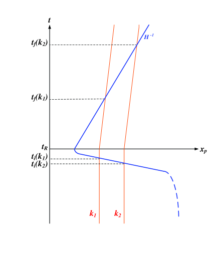
Figure 5: Space-time diagram (sketch) showing the evolution of fixed comoving scales in string gas cosmology. The vertical axis is time, the horizontal axis is physical distance. The solid curve represents the Einstein frame Hubble radius $H^{-1}$ which shrinks abruptly to a microphysical scale at $t_{R}$ and then increases linearly in time for $t>t_{R}$. Fixed comoving scales (the dotted lines labeled by $k_{1}$ and $k_{2}$) which are currently probed in cosmological observations have wavelengths which are smaller than the Hubble radius before $t_{R}$. They exit the Hubble radius at times $t_{i}(k)$ just prior to $t_{R}$, and propagate with a wavelength larger than the Hubble radius until they reenter the Hubble radius at times $t_{f}(k)$.

In contrast, in inflationary cosmology (Figure 1) the Hubble radius is constant during inflation ($t<t_{R}$, where here $t_{R}$ is the time of inflationary reheating), whereas the physical wavelength corresponding to a fixed comoving scale expands exponentially. Thus, as long as the period of inflation is sufficiently long, all scales of interest for current cosmological observations are sub-Hubble at the beginning of inflation.

There are both important similarities and key differences between the structure formation mechanisms in inflationary cosmology and string gas cosmology. In both cases, scales are sub-Hubble during the early stages, thus allowing for a causal generation mechanism. Also, in both cases the fluctuations evolve on super-Hubble scales for a long time in the radiation phase of standard cosmology, thus leading to their squeezing, which in turn leads to the phase coherence of the fluctuations which generate the acoustic oscillations in the angular power spectrum of the CMB. However, the actual generation mechanism for fluctuations is completely different. In inflationary cosmology, any thermal fluctuations present before the onset of inflation are red-shifted away, leaving us with a quantum vacuum state, whereas in the quasi-static Hagedorn phase of string gas cosmology matter is in a thermal state. Hence, whereas in inflationary cosmology the fluctuations originate as quantum vacuum perturbations, in string gas cosmology the inhomogeneities are created by the thermal fluctuations of the string gas.

As we have shown in [124, 125, 126], string thermodynamical fluctuations in the Hagedorn phase of string gas cosmology yield an almost scale-invariant spectrum of both scalar and tensor modes. This result stems from the holographic scaling of the specific heat $C_{V}(R)$ (evaluated for fixed volume) as a function of the radius $R$ of the box

$$C_{V}(R)\,\sim\,R^{2}\,.$$ (111)

As derived in [127], this result holds true for a gas of closed strings in a space-time in which the three large spatial dimensions are compact (see [130, 131] for recent papers emphasizing the role of holography). The scaling (111) is an intrinsically stringy result: thermal fluctuations of a gas of particles would lead to a very different scaling.

Since the primordial perturbations in our scenario are of thermal origin (and there are no non-vanishing chemical potentials), they will be adiabatic. The spectrum of scalar metric fluctuations has a slight red tilt. As a distinctive feature [128], our scenario predicts a slight blue tilt for the spectrum of gravitational waves. The red tilt for the scalar modes is due to the fact that the temperature when short wavelength modes exit the Hubble radius is slightly lower than the temperature when longer wavelength modes exit. The gravitational wave amplitude, in contrast, is determined by the pressure. Since the pressure is closer to zero the deeper in the Hagedorn phase we are, a slight blue tilt for the tensor fluctuations results. These results are explained in more detail in a recent review [110] and in the original references. Here, we will only focus on some of the key steps.

Our approximation scheme for computing the cosmological perturbations and gravitational wave spectra from string gas cosmology is as follows (the analysis is similar to how the calculations were performed in [55, 56] in the case of inflationary cosmology). For a fixed comoving scale $k$ we follow the matter fluctuations until the time $t_{i}(k)$ shortly before the end of the Hagedorn phase when the scale exits the Hubble radius At that time, we use the Einstein constraint equations (discussed below) to compute the values of $\Phi(k)$ and $h(k)$ ($h$ is the amplitude of the gravitational wave tensor), and then we propagate the metric fluctuations according to the standard gravitational perturbation equations until scales re-enter the Hubble radius at late times.

The first key point is to show how the scalar and tensor metric fluctuations can be extracted from knowledge of the energy-momentum tensor of the string gas. Working in conformal time $\eta$ and in the longitudinal gauge for the scalar metric fluctuations, the metric of a homogeneous and isotropic background space-time perturbed by linear cosmological perturbations and gravitational waves can be written in the form

$$ds^{2}=a^{2}(\eta)\left\{(1+2\Phi)d\eta^{2}-[(1-2\Phi)\delta_{ij}+h_{ij}]dx^{i}dx^{j}\right\}\,.$$ (112)

Here, $\Phi$ (which is a function of space and time) describes the scalar metric fluctuations . The tensor $h_{ij}$ is transverse and traceless and contains the two polarization states of the gravitational waves. We have assumed that there is no anisotropic stress.

Inserting the metric (112) into the Einstein equations, subtracting the background terms and truncating the perturbative expansion at linear order leads to the following system of equations

$$-3{\cal H}\left({\cal H}\Phi+\Phi^{{}^{\prime}}\right)+\nabla^{2}\Phi\, = \,4\pi Ga^{2}\delta T^{0}{}_{0}$$

$$\left({\cal H}\Phi+\Phi^{{}^{\prime}}\right)_{,i}\, = 4\pi Ga^{2}\delta T^{0}{}_{i}$$

$$\left[\left(2{\cal H}^{{}^{\prime}}+{\cal H}^{2}\right)\Phi+3{\cal H}\Phi^{{}^{\prime}}+\Phi^{{}^{\prime\prime}}\right] = -4\pi Ga^{2}\delta T^{i}{}_{i}\,,$$

$$-{1\over 2}\left[{{\cal H}^{\prime}}+{1\over 2}{\cal H}^{2}\right]h_{ij}+{1\over 4}{\cal H}h_{ij}^{\prime}$$

$$+\left[{{\partial^{2}}\over{\partial\eta^{2}}}-\nabla^{2}\right]h_{ij}\, = -4\pi Ga^{2}\delta T^{i}{}_{j}\,,$$ (113)

$$\mbox{for $i\neq j$}\,.$$

In the Hagedorn phase, these equations simplify substantially and allow us to extract the scalar and tensor metric fluctuations individually. Replacing comoving by physical coordinates, we obtain from the $00$ equation

$$\nabla^{2}\Phi\,=\,4\pi G\delta T^{0}{}_{0}\,$$ (114)

and from the $i\neq j$ equation

$$\nabla^{2}h_{ij}\,=\,-4\pi G\delta T^{i}{}_{j}\,.$$ (115)

The above equations (114) and (115) allow us to compute the power spectra of scalar and tensor metric fluctuations in terms of correlation functions of the string energy-momentum tensor. Since the metric perturbations are small in amplitude we can consistently work in Fourier space. Specifically,

$$\langle|\Phi(k)|^{2}\rangle\,=\,16\pi^{2}G^{2}k^{-4}\langle\delta T^{0}{}_{0}(k)\delta T^{0}{}_{0}(k)\rangle\,,$$ (116)

where the pointed brackets indicate expectation values, and

$$\langle|h(k)|^{2}\rangle\,=\,16\pi^{2}G^{2}k^{-4}\langle\delta T^{i}{}_{j}(k)\delta T^{i}{}_{j}(k)\rangle\,,$$ (117)

where on the right hand side of (117) we mean the average over the correlation functions with $i\neq j$.

The second key step is to compute the matter fluctuations in the Hagedorn phase. Since this phase is dominated by the gas of strings, fluctuations in our scenario are the thermal fluctuations of a string gas. We will consider a gas of closed strings in a compact space, i.e. our three-dimensional space is considered to be large but compact. Specifically, it is important to have winding modes in the spectrum of string states.

General thermodynamical relations allow us to compute the matter correlation functions in terms of the the specific heat $C_{V}$ and the pressure $p$. The result for the energy density fluctuation is

$$\langle\delta\rho^{2}\rangle\,=\,-\frac{1}{R^{6}}\frac{\partial}{\partial\beta}\left(F+\beta\frac{\partial F}{\partial\beta}\right)\,=\,\frac{T^{2}}{R^{6}}C_{V}\,,$$ (118)

where $F$ is the free energy of the string gas and $\beta$ is the inverse temperature. The off-diagonal pressure fluctuations, in turn, are given by

$$\langle\delta{T^{i}{}_{j}}^{2}\rangle\, = \,\langle{T^{i}{}_{j}}^{2}\rangle-\langle T^{i}{}_{j}\rangle^{2}$$

$$= \,\frac{1}{\beta R^{3}}\frac{\partial}{\partial\ln{R}}\left(-\frac{1}{R^{3}}\frac{\partial F}{\partial\ln{R}}\right)=\frac{1}{\beta R^{2}}\frac{\partial p}{\partial R}\,.$$

Now, we apply these relations to the thermodynamics of strings. In [127], the thermodynamical properties of a gas of closed strings in a toroidal space of radius $R$ were computed. To compute the fluctuations in a region of radius $R$ which forms part of our three-dimensional compact space, we will apply the results of [127] to a box of strings in a volume $V=R^{3}$.

The starting point of the computation is the formula for the density of states $\Omega(E,R)$ which then determines the cpecific heat and the pressure. The result for the specific heat is

$$C_{V}\,\approx\,2\frac{R^{2}/\ell^{3}}{T\left(1-T/T_{H}\right)}\,.$$ (120)

The ‘holographic’ scaling $C_{V}(R)\sim R^{2}$ is responsible for the overall scale-invariance of the spectrum of cosmological perturbations. The factor $(1-T/T_{H})$ in the denominator is responsible for giving the spectrum a slight red tilt.

For the pressure. we obtain

$$p(E,R)\approx n_{H}T_{H}-\frac{2}{3}\frac{(1-T/T_{H})}{\ell_{s}^{3}R}\ln{\left[\frac{\ell_{s}^{3}T}{R^{2}(1-T/T_{H})}\right]}\,,$$ (121)

which immediately yields

$$\langle\delta{T^{i}{}_{j}}^{2}\rangle\,\simeq\,\frac{T(1-T/T_{H})}{\ell_{s}^{3}R^{4}}\ln^{2}{\left[\frac{R^{2}}{\ell_{s}^{2}}(1-T/T_{H})\right]}\,.$$ (122)

Note that the factor $(1-T/T_{H})$ (which appears in the numerator of the key term in the expression for the microcanonical partition function) is in the numerator, whereas it was in the denominator in the expression for the specific heat. The reason is that in deriving the specific heat from the microcanonical partition function, a temperature derivative was taken, but not so in deriving the pressure. This leads to the slight blue tilt of the spectrum of gravitational waves, characteristic of our proposed structure formation scenario. As mentioned earlier, the physical reason for this blue tilt is that larger wavelength modes exit the Hubble radius deeper in the Hagedorn phase where the pressure is smaller and thus the strength of the tensor modes is less.

The third key step in the analysis is to compute the power spectra for the scalar and tensor modes based on the earlier results. The power spectrum of scalar metric fluctuations is given by

$$P_{\Phi}(k)\, \equiv \,{1\over{2\pi^{2}}}k^{3}|\Phi(k)|^{2}$$

$$= \,8G^{2}k^{-1}<|\delta\rho(k)|^{2}>\,.$$

$$= \,8G^{2}k^{2}<(\delta M)^{2}>_{R}$$

$$= \,8G^{2}k^{-4}<(\delta\rho)^{2}>_{R}\,,$$

where in the first step we have used (116) to replace the expectation value of $|\Phi(k)|^{2}$ in terms of the correlation function of the energy density, and in the second step we have made the transition to position space (note that $k=R^{-1}$).

According to (118), the density correlation function is given by the specific heat via $T^{2}R^{-6}C_{V}$. Inserting the expression from (120) for the specific heat of a string gas on a scale $R$ yields to the final result

$$P_{\Phi}(k)\,=\,8G^{2}{T\over{\ell_{s}^{3}}}{1\over{1-T/T_{H}}}$$ (124)

for the power spectrum of cosmological fluctuations. In the above equation, the temperature $T$ is to be evaluated at the time $t_{i}(k)$ when the mode $k$ exits the Hubble radius. Since modes with larger values of $k$ exit the Hubble radius slightly later when the temperature is slightly lower, a small red tilt of the spectrum is induced. The amplitude ${\cal A}_{S}$ of the power spectrum is given by

$${\cal A}_{S}\,\sim\,\bigl{(}{{l_{pl}}\over{l_{s}}}\bigr{)}^{4}{1\over{1-T/T_{H}}}\,.$$ (125)

Taking the last factor to be of order unity, we find that a string length three orders of magnitude larger than the Planck length, a string length which was assumed in early studies of string theory, gives the correct amplitude of the spectrum. Thus, it appears that the string gas cosmology structure formation mechanism does not have a serious amplitude problem.

Similarly, we can compute the power spectrum of the gravitational waves and obtain

$$P_{h}(k)\,\sim\,8G^{2}{T\over{\ell_{s}^{3}}}(1-T/T_{H})\ln^{2}{\left[\frac{1}{\ell_{s}^{2}k^{2}}(1-T/T_{H})^{-1}\right]}\,.$$ (126)

This shows that the spectrum of tensor modes is - to a first approximation, namely neglecting the logarithmic factor and neglecting the k-dependence of $T(t_{i}(k))$ - scale-invariant. The k-dependence of the temperature at Hubble radius crossing induces a small blue tilt for the spectrum of gravitational waves.

Comparing (124) and (126) we see that the tensor to scalar ratio is suppressed by the factor $(1-T/T_{H})^{2}$. Given a good understanding of the exit from the Hagedorn phase we would be able to compute this ratio as well as the magnitude of the spectral tilts for both scalar and tensor modes.

4.4 Discussion

In order to put our structure formation scenario on a firm basis, we need a consistent description of the Hagedorn phase. The dilaton gravity background allows us to understand the onset of the Hagedorn phase (going backwards in time), but since the dilaton blows up, we rapidly leave the domain of applicability of the model.

A background in which our string gas structure formation scenario can be implemented [113] is the ghost-free and asymptotically free higher derivative gravity model proposed in [94] given by the gravitational action

$$S\,=\,\int d^{4}x\sqrt{-g}F(R)$$ (127)

with

$$F(R)\,=\,R+\sum_{n=0}^{\infty}{{c_{n}}\over{M_{s}^{2n}}}R\bigl{(}{{\partial^{2}}\over{\partial^{2}t}}-\nabla^{2}\bigr{)}^{n}R\,,$$ (128)

where $M_{s}$ is the string mass scale (more generally, it is the scale where non-perturbative effects start to dominate), and the $c_{n}$ are coefficients of order unity.

As shown in [94] and [113], this action has bouncing cosmological solutions. If the temperature during the bounce phase is sufficiently high, then a gas of strings will be excited in this phase. In the absence of initial cosmological perturbations in the contracting phase, our string gas structure formation scenario is realized. The string network will contain winding modes in the same way that a string network formed during a cosmological phase transition will contain infinite strings. The dilaton is fixed in this scenario, thus putting the calculation of the cosmological perturbations on a firm basis. There are no additional dynamical degrees of freedom compared to those in Einstein gravity. The higher derivative corrections to the equations of motion (in particular to the Poisson equation) are suppressed by factors of $(k/M_{s})^{2}$. Thus, all of the conditions on a cosmological backgroound to successfully realize the string gas cosmology structure formation scenario are realized.

5 Conclusions

These lectures have focused on three topics in theoretical cosmology. The first is the inflationary universe scenario, the current paradigm of early universe cosmology. Inflation has been an extremely successful scenario. It explains why the universe is spatially flat and isotropic to the extent it is observed to be, and why it is so large and contains such a large amount of entropy, thus resolving several mysteries which the previous paradigm of cosmology, the SBB model, was not able to explain. Possibly more importantly, inflation provides a causal mechanism for the origin of the fluctuations which are now mapped out to great accuracy by recent cosmological observations. Inflation correctly (and fifteen years before the precision observations) predicted the power spectrum of CMB anisotropies.

The theory of cosmological perturbations is the key tool which allows us to take theories of the very early universe and calculate predictions for late time cosmology. This theory is applicable whatever the paradigm of early universe cosmology might be, and it is the second topic discussed in these lectures.

In spite of the successes of the inflationary universe scenario, key conceptual questions remain, making it clear that new input from fundamental physics is required in order to develop a better theory of the very early universe. The third topic discussed in these lectures, string gas cosmology, is an attempt to explore possible consequences for cosmology of superstring theory, the likely candidate for the new physics required for early universe cosmology. In particular, an alternative structure formation scenario not requiring inflationary dynamics emerges.

Acknowledgements

I wish to thank the organizers of the summer school for inviting me to lecture and for their hospitality in Dubrovnik. My research is supported by funds from NSERC and from the Canada Research Chair program.

References

- [1]
- [2] W. J. Percival et al. [The 2dFGRS Collaboration], “The 2dF Galaxy Redshift Survey: The power spectrum and the matter content of the universe,” Mon. Not. Roy. Astron. Soc. 327, 1297 (2001) [arXiv:astro-ph/0105252].
- [3] C. Stoughton et al. [SDSS Collaboration], “The Sloan Digital Sky Survey: Early data release,” Astron. J. 123, 485 (2002).
- [4] C. L. Bennett et al., “First Year Wilkinson Microwave Anisotropy Probe (WMAP) Observations: Preliminary Maps and Basic Results,” Astrophys. J. Suppl. 148, 1 (2003) [arXiv:astro-ph/0302207].
- [5] A. Vilenkin and E.P.S. Shellard; Cosmic Strings and Other Topological Defects, (Cambridge Univ. Press, Cambridge, 1994).
- [6] M. B. Hindmarsh and T. W. Kibble, “Cosmic strings,” Rept. Prog. Phys. 58, 477 (1995) [arXiv:hep-ph/9411342].
- [7] R. H. Brandenberger, “Topological defects and structure formation,” Int. J. Mod. Phys. A 9, 2117 (1994) [arXiv:astro-ph/9310041].
- [8] C. P. Burgess, “Inflatable string theory?,” Pramana 63, 1269 (2004) [arXiv:hep-th/0408037].
- [9] J. M. Cline, “Inflation from string theory,” arXiv:hep-th/0501179.
- [10] A. Linde, “Inflation and string cosmology,” eConf C040802, L024 (2004) [arXiv:hep-th/0503195].
- [11] J. C. Mather et al., “A Preliminary Measurement Of The Cosmic Microwave Background Spectrum By The Cosmic Background Explorer (Cobe) Satellite,” Astrophys. J. 354, L37 (1990).
- [12] H. Gush, M. Halpern and E. Wishnow, “Rocket Measurement of the Cosmic-Background-Radiation mm-Wave Spectrum”, Phys. Rev. Lett. 65, 537 (1990).
- [13] A. H. Guth, “The Inflationary Universe: A Possible Solution To The Horizon And Flatness Problems,” Phys. Rev. D 23, 347 (1981).
- [14] K. Sato, “First Order Phase Transition Of A Vacuum And Expansion Of The Universe,” Mon. Not. Roy. Astron. Soc. 195, 467 (1981).
- [15] R. Brout, F. Englert and E. Gunzig, “The Creation Of The Universe As A Quantum Phenomenon,” Annals Phys. 115, 78 (1978).
- [16] A. A. Starobinsky, “A New Type Of Isotropic Cosmological Models Without Singularity,” Phys. Lett. B 91, 99 (1980).
-
[17]
V. F. Mukhanov and G. V. Chibisov,
“Quantum Fluctuation And ’Nonsingular’ Universe. (In Russian),”
JETP Lett. 33, 532 (1981)
[Pisma Zh. Eksp. Teor. Fiz. 33, 549 (1981)];
- [18] W. Press, “Spontaneous production of the Zel’dovich spectrum of cosmological fluctuations”, Phys. Scr. 21, 702 (1980).
- [19] C. Armendariz-Picon, T. Damour and V. Mukhanov, “k-inflation,” Phys. Lett. B 458, 209 (1999) [arXiv:hep-th/9904075].
- [20] R. H. Brandenberger and J. H. Kung, “Chaotic Inflation As An Attractor In Initial Condition Space,” Phys. Rev. D 42, 1008 (1990).
- [21] D. S. Goldwirth and T. Piran, “Initial conditions for inflation,” Phys. Rept. 214, 223 (1992).
-
[22]
S. R. Coleman,
“The Fate Of The False Vacuum. 1. Semiclassical Theory,”
Phys. Rev. D 15, 2929 (1977)
[Erratum-ibid. D 16, 1248 (1977)];
C. G. . Callan and S. R. Coleman, “The Fate Of The False Vacuum. 2. First Quantum Corrections,” Phys. Rev. D 16, 1762 (1977). - [23] R. H. Brandenberger, “Quantum Field Theory Methods And Inflationary Universe Models,” Rev. Mod. Phys. 57, 1 (1985).
- [24] S. Dodelson, W. H. Kinney and E. W. Kolb, “Cosmic microwave background measurements can discriminate among inflation models,” Phys. Rev. D 56, 3207 (1997) [arXiv:astro-ph/9702166].
-
[25]
A. D. Linde,
Flatness, Homogeneity, Isotropy And Primordial Monopole Problems,”
Phys. Lett. B 108, 389 (1982);
A. Albrecht and P. J. Steinhardt, “Cosmology For Grand Unified Theories With Radiatively Induced Symmetry Breaking,” Phys. Rev. Lett. 48, 1220 (1982). - [26] S. R. Coleman and E. Weinberg, “Radiative Corrections As The Origin Of Spontaneous Symmetry Breaking,” Phys. Rev. D 7, 1888 (1973).
- [27] R. Brandenberger, G. Geshnizjani and S. Watson, “On the initial conditions for brane inflation,” Phys. Rev. D 67, 123510 (2003) [arXiv:hep-th/0302222].
- [28] A. D. Linde, “Chaotic Inflation,” Phys. Lett. B 129, 177 (1983).
- [29] A. Linde, “Prospects of inflation,” arXiv:hep-th/0402051.
-
[30]
H. A. Feldman and R. H. Brandenberger,
“Chaotic Inflation With Metric And Matter Perturbations,”
Phys. Lett. B 227, 359 (1989);
R. H. Brandenberger, H. Feldman and J. Kung, “Initial Conditions For Chaotic Inflation,” Phys. Scripta T36, 64 (1991). - [31] A. D. Linde, “Hybrid inflation,” Phys. Rev. D 49, 748 (1994) [arXiv:astro-ph/9307002].
- [32] J. Polchinski, “Introduction to cosmic F- and D-strings,” arXiv:hep-th/0412244.
- [33] A. D. Dolgov and A. D. Linde, “Baryon Asymmetry In Inflationary Universe,” Phys. Lett. B 116, 329 (1982).
- [34] L. F. Abbott, E. Farhi and M. B. Wise, “Particle Production In The New Inflationary Cosmology,” Phys. Lett. B 117, 29 (1982).
- [35] J. H. Traschen and R. H. Brandenberger, “Particle Production During Out-Of-Equilibrium Phase Transitions,” Phys. Rev. D 42, 2491 (1990).
- [36] L. Kofman, A. D. Linde and A. A. Starobinsky, “Reheating after inflation,” Phys. Rev. Lett. 73, 3195 (1994) [arXiv:hep-th/9405187].
- [37] Y. Shtanov, J. H. Traschen and R. H. Brandenberger, “Universe reheating after inflation,” Phys. Rev. D 51, 5438 (1995) [arXiv:hep-ph/9407247].
- [38] L. Kofman, A. D. Linde and A. A. Starobinsky, “Towards the theory of reheating after inflation,” Phys. Rev. D 56, 3258 (1997) [arXiv:hep-ph/9704452].
- [39] A. Liddle and D. Lyth, Cosmological Inflation and Large-Scale Structure, (Cambridge Univ. Press, Cambridge, 2000).
- [40] V. F. Mukhanov, H. A. Feldman and R. H. Brandenberger, “Theory Of Cosmological Perturbations. Part 1. Classical Perturbations. Part 2. Quantum Theory Of Perturbations. Part 3. Extensions,” Phys. Rept. 215, 203 (1992).
- [41] R. H. Brandenberger, “Lectures on the theory of cosmological perturbations,” Lect. Notes Phys. 646, 127 (2004) [arXiv:hep-th/0306071].
- [42] E. R. Harrison, “Fluctuations At The Threshold Of Classical Cosmology,” Phys. Rev. D 1, 2726 (1970).
- [43] Y. B. Zeldovich, “A Hypothesis, Unifying The Structure And The Entropy Of The Universe,” Mon. Not. Roy. Astron. Soc. 160, 1 (1972).
- [44] N. Afshordi and R. H. Brandenberger, “Super-Hubble nonlinear perturbations during inflation,” Phys. Rev. D 63, 123505 (2001) [arXiv:gr-qc/0011075].
-
[45]
E. Lifshitz,
“On The Gravitational Stability Of The Expanding Universe,”
J. Phys. (USSR) 10, 116 (1946);
E. M. Lifshitz and I. M. Khalatnikov, “Investigations In Relativistic Cosmology,” Adv. Phys. 12, 185 (1963). - [46] J. M. Bardeen, “Gauge Invariant Cosmological Perturbations,” Phys. Rev. D 22, 1882 (1980).
- [47] W. Press and E. Vishniac, “Tenacious myths about cosmological perturbations larger than the horizon size,” Astrophys. J. 239, 1 (1980).
- [48] H. Kodama and M. Sasaki, “Cosmological Perturbation Theory,” Prog. Theor. Phys. Suppl. 78, 1 (1984).
- [49] M. Bruni, G. F. Ellis and P. K. Dunsby, “Gauge invariant perturbations in a scalar field dominated universe,” Class. Quant. Grav. 9, 921 (1992).
- [50] J. c. Hwang, “Evolution of ideal fluid cosmological perturbations,” Astrophys. J. 415, 486 (1993).
- [51] R. Durrer, “Anisotropies in the cosmic microwave background: Theoretical foundations,” Helv. Phys. Acta 69, 417 (1996) [arXiv:astro-ph/9610234].
- [52] J. Stewart, “Perturbations of Friedmann-Robertson-Walker Cosmological Models”, Class. Quant. Grav. 7, 1169 (1990).
- [53] J. Stewart and M. Walker, “Perturbations Of Spacetimes In General Relativity,” Proc. Roy. Soc. Lond. A 341, 49 (1974).
- [54] R. Durrer and M. Sakellariadou, “A New contribution to cosmological perturbations of some inflationary models,” Phys. Rev. D 50, 6115 (1994) [arXiv:astro-ph/9404043].
- [55] J. M. Bardeen, P. J. Steinhardt and M. S. Turner, “Spontaneous Creation Of Almost Scale - Free Density Perturbations In An Inflationary Universe,” Phys. Rev. D 28, 679 (1983).
- [56] R. H. Brandenberger and R. Kahn, “Cosmological Perturbations In Inflationary Universe Models,” Phys. Rev. D 29, 2172 (1984).
- [57] D. H. Lyth, “Large Scale Energy Density Perturbations And Inflation,” Phys. Rev. D 31, 1792 (1985).
- [58] F. Finelli and R. H. Brandenberger, “Parametric amplification of gravitational fluctuations during reheating,” Phys. Rev. Lett. 82, 1362 (1999) [arXiv:hep-ph/9809490].
- [59] B. A. Bassett and F. Viniegra, “Massless metric preheating,” Phys. Rev. D 62, 043507 (2000) [arXiv:hep-ph/9909353].
- [60] F. Finelli and R. H. Brandenberger, “Parametric amplification of metric fluctuations during reheating in two field models,” Phys. Rev. D 62, 083502 (2000) [arXiv:hep-ph/0003172].
- [61] S. Weinberg, “Adiabatic modes in cosmology,” Phys. Rev. D 67, 123504 (2003) [arXiv:astro-ph/0302326].
- [62] W. B. Lin, X. H. Meng and X. M. Zhang, “Adiabatic gravitational perturbation during reheating,” Phys. Rev. D 61, 121301 (2000) [arXiv:hep-ph/9912510].
- [63] A. H. Guth and S. Y. Pi, “Fluctuations In The New Inflationary Universe,” Phys. Rev. Lett. 49, 1110 (1982).
- [64] A. A. Starobinsky, “Dynamics Of Phase Transition In The New Inflationary Universe Scenario And Generation Of Perturbations,” Phys. Lett. B 117, 175 (1982).
- [65] S. W. Hawking, “The Development Of Irregularities In A Single Bubble Inflationary Universe,” Phys. Lett. B 115, 295 (1982).
- [66] V. F. Mukhanov, “Gravitational Instability Of The Universe Filled With A Scalar Field,” JETP Lett. 41, 493 (1985) [Pisma Zh. Eksp. Teor. Fiz. 41, 402 (1985)].
- [67] V. F. Mukhanov, “Quantum Theory Of Gauge Invariant Cosmological Perturbations,” Sov. Phys. JETP 67, 1297 (1988) [Zh. Eksp. Teor. Fiz. 94N7, 1 (1988 ZETFA,94,1-11.1988)].
- [68] M. Sasaki, “Large Scale Quantum Fluctuations In The Inflationary Universe,” Prog. Theor. Phys. 76, 1036 (1986).
-
[69]
V. N. Lukash, Pisma Zh. Eksp. Teor. Fiz. 31, 631 (1980);
V. N. Lukash, “Production Of Phonons In An Isotropic Universe,” Sov. Phys. JETP 52, 807 (1980) [Zh. Eksp. Teor. Fiz. 79, (1980)]. - [70] N. Birrell and P.C.W. Davies: Quantum Fields in Curved Space, (Cambridge Univ. Press, Cambridge, 1982).
- [71] R. H. Brandenberger, “Quantum Fluctuations As The Source Of Classical Gravitational Perturbations In Inflationary Universe,” Nucl. Phys. B 245, 328 (1984).
- [72] R. H. Brandenberger and C. T. Hill, “Energy Density Fluctuations In De Sitter Space,” Phys. Lett. B 179, 30 (1986).
- [73] D. Polarski and A. A. Starobinsky, “Semiclassicality and decoherence of cosmological perturbations,” Class. Quant. Grav. 13, 377 (1996) [arXiv:gr-qc/9504030].
- [74] R. A. Sunyaev and Y. B. Zeldovich, “Small scale fluctuations of relic radiation,” Astrophys. Space Sci. 7, 3 (1970).
- [75] P. J. E. Peebles and J. T. Yu, “Primeval adiabatic perturbation in an expanding universe,” Astrophys. J. 162, 815 (1970).
- [76] L. P. Grishchuk, “Amplification Of Gravitational Waves In An Istropic Universe,” Sov. Phys. JETP 40, 409 (1975) [Zh. Eksp. Teor. Fiz. 67, 825 (1974)].
-
[77]
A. D. Linde,
“Eternal Chaotic Inflation,”
Mod. Phys. Lett. A 1, 81 (1986);
A. D. Linde and D. A. Linde, “Topological defects as seeds for eternal inflation,” Phys. Rev. D 50, 2456 (1994) [arXiv:hep-th/9402115]. - [78] R. Allahverdi, K. Enqvist, J. Garcia-Bellido and A. Mazumdar, “Gauge invariant MSSM inflaton,” arXiv:hep-ph/0605035.
- [79] F. C. Adams, K. Freese and A. H. Guth, “Constraints On The Scalar Field Potential In Inflationary Models,” Phys. Rev. D 43, 965 (1991).
-
[80]
N. Turok and R. H. Brandenberger,
“Cosmic Strings And The Formation Of Galaxies And Clusters Of Galaxies,”
Phys. Rev. D 33, 2175 (1986);
H. Sato, “Galaxy Formation by Cosmic Strings,” Prog. Theor. Phys. 75, 1342 (1986);
A. Stebbins, “Cosmic Strings and Cold Matter”, Ap. J. (Lett.) 303, L21 (1986). -
[81]
A. Albrecht, D. Coulson, P. Ferreira and J. Magueijo,
“Causality and the microwave background,”
Phys. Rev. Lett. 76, 1413 (1996)
[arXiv:astro-ph/9505030];
J. Magueijo, A. Albrecht, D. Coulson and P. Ferreira, “Doppler peaks from active perturbations,” Phys. Rev. Lett. 76, 2617 (1996) [arXiv:astro-ph/9511042];
U. L. Pen, U. Seljak and N. Turok, “Power spectra in global defect theories of cosmic structure formation,” Phys. Rev. Lett. 79, 1611 (1997) [arXiv:astro-ph/9704165]. - [82] R. H. Brandenberger, “Inflationary cosmology: Progress and problems,” publ. in proc. of IPM School On Cosmology 1999: Large Scale Structure Formation, arXiv:hep-ph/9910410.
-
[83]
R. H. Brandenberger and J. Martin, “The robustness of inflation to changes in super-Planck-scale physics,”
Mod. Phys. Lett. A 16, 999 (2001),
[arXiv:astro-ph/0005432];
J. Martin and R. H. Brandenberger, “The trans-Planckian problem of inflationary cosmology,” Phys. Rev. D 63, 123501 (2001), [arXiv:hep-th/0005209]. -
[84]
J. C. Niemeyer,
“Inflation with a high frequency cutoff,”
Phys. Rev. D 63, 123502 (2001),
[arXiv:astro-ph/0005533];
S. Shankaranarayanan, “Is there an imprint of Planck scale physics on inflationary cosmology?,” Class. Quant. Grav. 20, 75 (2003), [arXiv:gr-qc/0203060];
J. C. Niemeyer and R. Parentani, “Trans-Planckian dispersion and scale-invariance of inflationary perturbations,” Phys. Rev. D 64, 101301 (2001), [arXiv:astro-ph/0101451]. - [85] W. G. Unruh, “Sonic analog of black holes and the effects of high frequencies on black hole evaporation,” Phys. Rev. D 51, 2827 (1995).
- [86] S. Corley and T. Jacobson, “Hawking Spectrum and High Frequency Dispersion,” Phys. Rev. D 54, 1568 (1996) [arXiv:hep-th/9601073].
- [87] R. H. Brandenberger and J. Martin, “Back-reaction and the trans-Planckian problem of inflation revisited,” Phys. Rev. D 71, 023504 (2005) [arXiv:hep-th/0410223].
- [88] T. Tanaka, “A comment on trans-Planckian physics in inflationary universe,” [arXiv:astro-ph/0012431].
- [89] A. A. Starobinsky, “Robustness of the inflationary perturbation spectrum to trans-Planckian physics,” Pisma Zh. Eksp. Teor. Fiz. 73, 415 (2001), [JETP Lett. 73, 371 (2001)], [arXiv:astro-ph/0104043].
- [90] S. Hawking and G. Ellis, The Large-Scale Structure of Space-Time (Cambridge Univ. Press, Cambridge, 1973).
- [91] A. Borde and A. Vilenkin, “Eternal inflation and the initial singularity,” Phys. Rev. Lett. 72, 3305 (1994) [arXiv:gr-qc/9312022].
- [92] N. Arkani-Hamed, L. Motl, A. Nicolis and C. Vafa, “The string landscape, black holes and gravity as the weakest force,” arXiv:hep-th/0601001.
-
[93]
R. H. Brandenberger, V. F. Mukhanov and A. Sornborger,
“A Cosmological theory without singularities,”
Phys. Rev. D 48, 1629 (1993)
[arXiv:gr-qc/9303001];
V. F. Mukhanov and R. H. Brandenberger, “A Nonsingular universe,” Phys. Rev. Lett. 68, 1969 (1992). - [94] T. Biswas, A. Mazumdar and W. Siegel, “Bouncing universes in string-inspired gravity,” JCAP 0603, 009 (2006) [arXiv:hep-th/0508194].
- [95] M. Bojowald, “Loop quantum cosmology,” Living Rev. Rel. 8, 11 (2005) [arXiv:gr-qc/0601085].
- [96] R. Hagedorn, “Statistical Thermodynamics Of Strong Interactions At High-Energies,” Nuovo Cim. Suppl. 3, 147 (1965).
- [97] R. H. Brandenberger and C. Vafa, “Superstrings In The Early Universe,” Nucl. Phys. B 316, 391 (1989).
- [98] R. H. Brandenberger, “Back reaction of cosmological perturbations and the cosmological constant problem,” publ. in the proc. of the 18th IAP Colloquium On The Nature Of Dark Energy: Observational And Theoretical Results On The Accelerating Universe, arXiv:hep-th/0210165.
- [99] P. Brax, C. van de Bruck and A. C. Davis, “Brane world cosmology,” Rept. Prog. Phys. 67, 2183 (2004) [arXiv:hep-th/0404011].
- [100] M. Majumdar and A.-C. Davis, “Cosmological creation of D-branes and anti-D-branes,” JHEP 0203, 056 (2002) [arXiv:hep-th/0202148].
- [101] R. Durrer, M. Kunz and M. Sakellariadou, “Why do we live in 3+1 dimensions?,” Phys. Lett. B 614, 125 (2005) [arXiv:hep-th/0501163].
- [102] A. Karch and L. Randall, “Relaxing to three dimensions,” Phys. Rev. Lett. 95, 161601 (2005) [arXiv:hep-th/0506053].
- [103] A. A. Tseytlin and C. Vafa, “Elements of string cosmology,” Nucl. Phys. B 372, 443 (1992) [arXiv:hep-th/9109048].
- [104] S. Alexander, R. H. Brandenberger and D. Easson, “Brane gases in the early universe,” Phys. Rev. D 62, 103509 (2000) [arXiv:hep-th/0005212].
- [105] S. Kalyana Rama, “A principle to determine the number (3+1) of large spacetime dimensions,” arXiv:hep-th/0610071.
- [106] J. Kripfganz and H. Perlt, “Cosmological Impact Of Winding Strings,” Class. Quant. Grav. 5, 453 (1988).
- [107] T. Battefeld and S. Watson, “String gas cosmology,” Rev. Mod. Phys. 78, 435 (2006) [arXiv:hep-th/0510022].
- [108] R. H. Brandenberger, “Challenges for string gas cosmology,” publ. in proc. of the 59th Yamada Conference On Inflating Horizon Of Particle Astrophysics And Cosmology, arXiv:hep-th/0509099.
- [109] R. H. Brandenberger, “Moduli stabilization in string gas cosmology,” Prog. Theor. Phys. Suppl. 163, 358 (2006) [arXiv:hep-th/0509159].
- [110] R. H. Brandenberger, “Conceptual Problems of Inflationary Cosmology and a New Approach to Cosmological Structure Formation,” arXiv:hep-th/0701111, to be publ. in the proceedings of Inflation + 25 (Springer, Berlin, 2007).
- [111] J. Polchinski, String Theory, Vols. 1 and 2, (Cambridge Univ. Press, Cambridge, 1998).
- [112] T. Boehm and R. Brandenberger, “On T-duality in brane gas cosmology,” JCAP 0306, 008 (2003) [arXiv:hep-th/0208188].
- [113] T. Biswas, R. Brandenberger, A. Mazumdar and W. Siegel, “Non-perturbative gravity, Hagedorn bounce and CMB,” arXiv:hep-th/0610274.
-
[114]
G. F. R. Ellis and R. Maartens,
“The emergent universe: Inflationary cosmology with no singularity,”
Class. Quant. Grav. 21, 223 (2004)
[arXiv:gr-qc/0211082];
G. F. R. Ellis, J. Murugan and C. G. Tsagas, “The emergent universe: An explicit construction,” Class. Quant. Grav. 21, 233 (2004) [arXiv:gr-qc/0307112]. - [115] R. Easther, B. R. Greene, M. G. Jackson and D. Kabat, “String windings in the early universe,” JCAP 0502, 009 (2005) [arXiv:hep-th/0409121].
- [116] R. Danos, A. R. Frey and A. Mazumdar, “Interaction rates in string gas cosmology,” Phys. Rev. D 70, 106010 (2004) [arXiv:hep-th/0409162].
- [117] S. Watson and R. H. Brandenberger, “Isotropization in brane gas cosmology,” Phys. Rev. D 67, 043510 (2003) [arXiv:hep-th/0207168].
- [118] G. Veneziano, “Scale factor duality for classical and quantum strings,” Phys. Lett. B 265, 287 (1991).
- [119] M. Maggiore and A. Riotto, “D-branes and cosmology,” Nucl. Phys. B 548, 427 (1999) [arXiv:hep-th/9811089].
- [120] R. H. Brandenberger et al., “More on the spectrum of perturbations in string gas cosmology,” JCAP 0611, 009 (2006) [arXiv:hep-th/0608186].
- [121] S. Arapoglu, A. Karakci and A. Kaya, “S-duality in string gas cosmology,” arXiv:hep-th/0611193.
- [122] R. Brandenberger, D. A. Easson and D. Kimberly, “Loitering phase in brane gas cosmology,” Nucl. Phys. B 623, 421 (2002) [arXiv:hep-th/0109165].
- [123] R. Brandenberger and N. Shuhmaher, “The Confining Heterotic Brane Gas: A Non-Inflationary Solution to the Entropy and Horizon Problems of Standard Cosmology,” JHEP 0601, 074 (2006) [arXiv:hep-th/0511299].
- [124] A. Nayeri, R. H. Brandenberger and C. Vafa, “Producing a scale-invariant spectrum of perturbations in a Hagedorn phase of string cosmology,” Phys. Rev. Lett. 97, 021302 (2006) [arXiv:hep-th/0511140].
- [125] A. Nayeri, “Inflation free, stringy generation of scale-invariant cosmological fluctuations in D = 3 + 1 dimensions,” arXiv:hep-th/0607073.
- [126] R. H. Brandenberger, A. Nayeri, S. P. Patil and C. Vafa, “String gas cosmology and structure formation,” arXiv:hep-th/0608121.
- [127] N. Deo, S. Jain, O. Narayan and C. I. Tan, “The Effect of topology on the thermodynamic limit for a string gas,” Phys. Rev. D 45, 3641 (1992).
- [128] R. H. Brandenberger, A. Nayeri, S. P. Patil and C. Vafa, “Tensor modes from a primordial Hagedorn phase of string cosmology,” arXiv:hep-th/0604126.
- [129] N. Kaloper, L. Kofman, A. Linde and V. Mukhanov, “On the new string theory inspired mechanism of generation of cosmological perturbations,” JCAP 0610, 006 (2006) [arXiv:hep-th/0608200].
- [130] J. Magueijo, L. Smolin and C. R. Contaldi, “Holography and the scale-invariance of density fluctuations,” arXiv:astro-ph/0611695.
- [131] S. Patil and A. Mazumdar, in preparation (2007).