Quasi-solvability of Calogero-Sutherland model with Anti-periodic Boundary Condition

Abstract

The $U(1)$ Calogero-Sutherland Model with anti-periodic boundary condition is studied. This model is obtained by applying a vertical magnetic field perpendicular to the plane of one dimensional ring of particles. The trigonometric form of the Hamiltonian is recast by using a suitable similarity transformation. The transformed Hamiltonian is shown to be integrable by constructing a set of momentum operators which commutes with the Hamiltonian and amongst themselves. The function space of monomials of several variables remains invariant under the action of these operators. The above properties imply the quasi-solvability of the Hamiltonian under consideration.

I Introduction

The study of Calogero-Sutherland system has inspired significant research activity since the pioneering work of Calogero and Sutherland cal62 ; suth71 . The integrability of the model has been studied for different root systems over the past few decades ols83 . A few of the classical and spin varieties of the model are found to be exactly solvable and the solutions in terms of their eigenvalues and eigenfunctions have been used extensively to describe physical properties of several condensed matter systems. The study of Calogero systems is also related to various other research areas in physics and mathematics, e.g., Yang-Mills theories gor94 ; mina94 , soliton theory poly95 , random matrix model dyson62 , multivariable orthogonal polynomials jack69 , Selberg integral formula forr93 , $W^{\infty}$ algebra hika93 etc.

This article investigates the Calogero-Sutherland Model (CSM) with anti-periodic boundary condition. The anti-periodic boundary condition is a special case of the general twisted boundary condition which arises when a one dimensional chain of particles is placed in a transverse magnetic field. A one dimensional chain of particles with a periodic boundary condition is topologically equivalent to a one dimensional ring. A particle transported adiabatically around this ring an integral number of times returns to the same point. In absence of a magnetic field this implies that the particle returns to the same quantum state. However, in the presence of a transverse magnetic field, one adiabatic transportation around the ring introduces a phase factor $\exp(i\phi)$. This is called a twisted boundary condition. When the phase factor is $\exp(i\phi)=-1$, it is called an anti-periodic boundary condition. Though the introduction of a magnetic field is physically important in this context, the model becomes mathematically more involved; and the CSM with anti-periodic boundary condition remains less extensively investigated.

The original version of the Calogero system incorporates long-range interaction by considering a two-body inverse square potential. The integrability of such systems was initially studied by Calogero and Perelomov cal75 ; perel77 by means of Lax pair formulation. The integrability of CSM has since been investigated in a variety of ways ols83 ; mina93 ; berm97 ; poly99 .

The general form of CSM Hamiltonian is often represented by the following equation:

$$H_{N}=\sum_{j=1}^{N}{\partial_{j}}^{2}-\lambda(\lambda-1)\sum_{\stackrel{{\scriptstyle\scriptstyle{j,k}}}{{j\neq k}}}U(x_{jk}^{-})$$ (1)

The two-body potential, represented by $U(x_{jk}^{-})$ is a long-range interaction in a chain of spinless nonrelativistic particles in one dimension. Here, $\lambda$ is a dimensionless interaction parameter, $x_{j}$ and $x_{k}$ denote the coordinates of the $j$-th and $k$-th particle respectively and $x_{jk}^{-}=x_{j}-x_{k}$. While studying the solvability of $A_{N-1}$-type Calogero model, the Hamiltonian is operated on a partially ordered state space of all symmetric polynomials of several variables. This results in an upper triangular representation of the Hamiltonian. The diagonal terms of this matrix are the eigenvalues of the Hamiltonian. The orthonormal eigenfunctions are expressed in terms of Jack symmetric polynomials jack69 which are very useful in determining the various physical properties of many particle systems with long-range interactions habook .

The search for an exact form of eigenfunction sometimes leads to partial diagonalization of the Hamiltonian tana05 ; fin01 . Among the one dimensional systems with periodic boundary condition, several such quasi-solvable models exist. The eigenvalues and eigenfunctions for many of them have been obtainedtur87 ; ushbook . The model with $sl(2)$ structure was first discovered by Turbiner and Ushveridze tur88 . It was also observed that the well known $N$ body Calogero-Sutherland models cal71 ; suth71 ; ruhl95 have similar Lie algebraic structure of $sl(N+1)$.

It may be noted that these models are in fact different generalizations of the classically integrable Inozemtsev model tana04 ; ino83 . The common feature of these models with some underlying Lie algebraic structure is the existence of an invariant finite dimensional module of the associated Lie algebra. Post and Turbiner post95 studied a classification of linear differential operators of a single variable which have a finite dimensional invariant subspace spanned by monomials. One of the basic advantages of quasi-solvability is that, one can restrict the study to a finite dimensional submanifold of the full Hamiltonian. The finite dimensional matrix elements can be calculated by allowing the Hamiltonian to act on finite-dimensional subspaces of a Hilbert space on which it is originally defined. When the Hamiltonian operator preserves an infinite number of subsequences of such finite dimensional subspaces tana05 it becomes solvable. The exact solvability of a model is ensured when the closure property is imposed on the space on which the Hamiltonian is allowed to act.

In this article we study the integrability and solvability of a spinless non-relativistic Calogero-Sutherland model (CSM) with anti-periodic boundary condition. The two-body long-range interaction incorporating the anti-periodic boundary condition is derived. The Hamiltonian so obtained is reduced to a more apparent integrable form, using a similarity transformation. The integrability is then verified by constructing a set of mutually commuting momentum-like differential operators which further commute with the Hamiltonian. Finally, the concept of quasi-solvability is discussed for a model of many particle system. For CSM with anti-periodic boundary condition the quasi-solvability is studied by operating the Hamiltonian on a multivariable polynomial space fin01 . The momentum operators in the anti-periodic model remind us of the well known Dunkl operator dunk89 ; che91 which resembles the Laplace-Beltrami-type operator acting on a symmetric Riemannian space. These operators are extensively used in the study of integrability and solvability of Calogero-Sutherland models. It is shown that these commuting momentum operators preserve the space spanned by all monomials of degree $n$, i.e., $\{\prod_{i}z_{i}^{\ell_{i}}\}$, where $\ell_{i}\geq 0$ and $\sum\ell_{i}=n$, $n$ being a non-negative integer. This property ensures the quasi-solvability of the Hamiltonian under study.

II Trigonometric version of CSM Hamiltonian

Let us first consider the periodic CSM with inverse square long-range interaction in the absence of a magnetic field. The topological representation of a one dimensional chain of particles with periodic boundary condition is simply a circular ring. A particle when transported adiabatically around the ring an integral number of times, does not take up any phase factor, and so the eigenfunctions retain their initial form. Then the pairwise interaction summed around a unitarily equivalent circle of circumference $L$, an infinite number of times is given as,

$$\sum_{n=-\infty}^{+\infty}\frac{1}{(x+nL)^{2}}=\frac{1}{d(x)^{2}}$$ (2)

where, as shown in the figure, $x$ is the interparticle distance along the ring and $d(x)$ is the chord length. It is easy to verify that $d(x)=L/\pi\sin(\pi x/L)$.

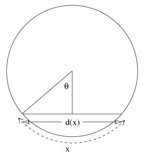
Figure 1: Inter-particle distances $d(x)$ and $d(x_{j+1}-x_{j})$ for particles on a circular chain

Therefore, the potential $U(x)=(\pi^{2}/L^{2})\sin^{-2}{x}$ is an inverse trigonometric function of the inter-particle distance $x$. The Hamiltonian with the above potential is given by,

$$H_{N}=\sum_{j=1}^{N}{\partial_{j}}^{2}-\lambda(\lambda-1)\frac{\pi^{2}}{L^{2}}\sum_{\stackrel{{\scriptstyle\scriptstyle{j,k}}}{{j\neq k}}}\frac{1}{\sin^{2}(\pi x_{jk}^{-}/L)}$$ (3)

where $x_{jk}^{-}=x_{j}-x_{k}$. Using standard trigonometric identity, making a change of variable $(\pi/2L)x_{j}\rightarrow x_{j}$ and rescaling the Hamiltonian $(4L^{2}/\pi^{2})H_{N}\rightarrow H_{N}$, Eq. (3) may be written as,

$$H_{N}=\sum_{j=1}^{N}{\partial_{j}}^{2}-\lambda(\lambda-1)\sum_{\stackrel{{\scriptstyle\scriptstyle{j,k}}}{{j\neq k}}}\left(\frac{1}{\sin^{2}{(x_{jk}^{-})}}+\frac{1}{\cos^{2}{(x_{jk}^{-})}}\right).$$ (4)

Let us now consider the anti-periodic case. When a magnetic field is introduced transverse to the one dimensional ring, a general twisted boundary condition arises. A particle transported adiabatically around the entire system $n$ number of times picks up a net phase $\exp{(in\phi)}$. The pairwise interaction summed around a unitarily equivalent circle of circumference $L$, an infinite number of times, is now given as,

$$\sum_{n=-\infty}^{+\infty}\frac{\exp(i\phi n)}{(x+nL)^{2}}.$$ (5)

The above summation can be performed by making the choice, $\phi=2\pi p/q$, with $p,\,q$ relative primes, and $n=jq+k$, with $j,\,k$ integers ($-\infty<j<+\infty$ and $0\leq k\leq q-1$). The interaction term becomes,

$$\sum_{n=-\infty}^{+\infty}\frac{\exp{(i\phi n)}}{(x+nL)^{2}}=\sum_{k=0}^{q-1}\sum_{j=-\infty}^{+\infty}\frac{\exp(i2\pi pj)\exp(i2\pi pk/q)}{\left[(x+kL)+(qL)j\right]^{2}}=\sum_{k=0}^{q-1}\frac{\exp{(i2\pi pk/q)}}{\left[(qL/\pi)\sin{\frac{\pi(x+kL)}{qL}}\right]^{2}}.$$ (6)

The last expression represents an interaction with a general twisted boundary condition. The model can be viewed as a system of interacting particles residing on a circle with circumference $qL$. For $p/q=1/2$ the sum becomes,

$$\sum_{k=0}^{q-1}\frac{\exp{(i2\pi pk/q)}}{\left[(qL/\pi)\sin{\frac{\pi(x+kL)}{qL}}\right]^{2}}\Longrightarrow\sum_{k=0}^{1}\frac{\exp{(i\pi k)}}{\left[(qL/\pi)\sin{\frac{\pi(x+kL)}{qL}}\right]^{2}}=\sum_{k=0}^{1}\frac{(-1)^{k}}{\left[(2L/\pi)\sin{\frac{\pi(x+kL)}{2L}}\right]^{2}}.$$ (7)

This corresponds to an anti-periodic boundary condition habook . The potential then takes the following form

$$U(x)=\frac{\cos{(\pi x/L)}}{(L^{2}/\pi^{2})\sin^{2}{(\pi x/L)}}.$$ (8)

Thus the Hamiltonian with anti-periodic boundary condition, using standard trigonometric identity, and scale changes $(\pi/2L)x_{j}\rightarrow x_{j}$ and $(4L^{2}/\pi^{2})H_{N}\rightarrow H_{N}$, becomes

$$H_{N}^{{}^{ap}}=\sum_{j=1}^{N}{\partial_{j}}^{2}-\lambda(\lambda-1)\sum_{\stackrel{{\scriptstyle\scriptstyle{j,k}}}{{j\neq k}}}\left(\frac{1}{\sin^{2}{(x_{jk}^{-})}}-\frac{1}{\cos^{2}{(x_{jk}^{-})}}\right).$$ (9)

III Integrability of the model Hamiltonian

The integrability of such types of Hamiltonian is established by constructing a complete set of commuting momentum operators that also commute with the model Hamiltonian. These operators were initially introduced in the study of Calogero-Sutherland model with periodic boundary conditions (both spin and classical cases) and are known as Dunkl operators. Similar operators have been used to study Calogero-Sutherland-type models derived from different root systems and are called Dunkl-type operators fin01 ; buch94 .

To construct commutative Dunkl-type operators we introduce variables, $z_{j}=\exp(2ix_{j})$. Using this substitution, the anti-periodic Hamiltonian becomes,

$$H_{N}^{{}^{ap}}=\sum_{j=1}^{N}(z_{j}\partial_{j})^{2}-\lambda(\lambda-1)\sum_{\stackrel{{\scriptstyle\scriptstyle{j,k}}}{{j\neq k}}}\frac{z_{j}z_{k}}{(z_{jk}^{-})^{2}}-\lambda(\lambda-1)\sum_{\stackrel{{\scriptstyle\scriptstyle{j,k}}}{{j\neq k}}}\frac{z_{j}z_{k}}{(z_{jk}^{+})^{2}},\;\;\;\mathrm{where}\;\;\;z_{jk}^{\pm}=z_{j}\pm z_{k}.$$ (10)

Let us apply the following similarity transformation,

$$\widetilde{H}_{N}=\Delta^{-1}H_{N}^{{}^{ap}}\Delta$$

where,

$$\Delta=\prod_{\stackrel{{\scriptstyle\scriptstyle{j,k}}}{{j<k}}}\frac{(z_{jk}^{-})^{\mu_{1}(\lambda)}(z_{jk}^{+})^{\mu_{2}(\lambda)}}{(z_{j}z_{k})^{(\{\mu_{1}(\lambda)+\mu_{2}(\lambda)\}/2)}},\;\;\mathrm{and}\;\;\mu_{1}(\lambda)=\lambda,1-\lambda\;,\;\;\;\mu_{2}(\lambda)=\frac{1}{2}[1\pm\sqrt{1+4\lambda-4\lambda^{2}}].$$

Thus, the anti-periodic Hamiltonian becomes

$$\widetilde{H}_{N}=\sum_{j=1}^{N}(z_{j}\partial_{j})^{2}+\frac{\mu_{1}(\lambda)}{2}\sum_{\stackrel{{\scriptstyle\scriptstyle{j,k}}}{{j\neq k}}}\frac{z_{jk}^{+}}{z_{jk}^{-}}(z_{j}\partial_{j}-z_{k}\partial_{k})+\frac{\mu_{2}(\lambda)}{2}\sum_{\stackrel{{\scriptstyle\scriptstyle{j,k}}}{{j\neq k}}}\frac{z_{jk}^{-}}{z_{jk}^{+}}(z_{j}\partial_{j}-z_{k}\partial_{k})$$ (11)

The term $\mu_{1}(\lambda)$ is real for all $\lambda$, however, $\mu_{2}(\lambda)$ is real only for $1+4\lambda-4\lambda^{2}\geq 0$, i.e., $|\lambda-\frac{1}{2}|\leq\frac{1}{\sqrt{2}}$. Under this restriction, the Hamiltonian $\widetilde{H}_{N}$ becomes hermitian. In the following, the integrability of the Hamiltonian is studied for different allowed values of $\lambda$.

Let us introduce the coordinate exchange operators $\{\Lambda_{jk}|j,k=1,..N;j\neq k\}$ and the sign reversing operators $\{\Lambda_{j}|j,k=1,..N\}$. The coordinate exchange operator acting on the coordinates of $j$-th and $k$-th particle may be defined by the operation $\Lambda_{jk}f(z_{1},..,z_{j},..,z_{k},..,z_{N})=f(z_{1},..,z_{k},..,z_{j},..,z_{N})$. This operator is (i) self-adjoint, (ii) unitary, and satisfies (iii) $\Lambda_{ij}\Lambda_{jk}=\Lambda_{ik}\Lambda_{ij}=\Lambda_{jk}\Lambda_{ik}$ , (iv) $\Lambda_{ij}\Lambda_{kl}=\Lambda_{kl}\Lambda_{ij}$ , (v) $\Lambda_{jk}z_{k}\partial_{k}=z_{j}\partial_{j}$ .

The sign reversing operator $\Lambda_{j}$ may be defined by its action on the coordinates of the $j$-th particle as $\Lambda_{j}f(z_{1},..,z_{j},..,z_{N})=f(z_{1},..,-z_{j},..,z_{N})$. This operator is (i) self-inverse $\Lambda_{j}^{-1}=\Lambda_{j}$, (ii) mutually commuting $[\Lambda_{j},\Lambda_{k}]=0$, and satisfies (iii) $[\Lambda_{ij},\Lambda_{k}]=0$ , $i\neq j\neq k$, (iv) $\Lambda_{ij}\Lambda_{j}=\Lambda_{i}\Lambda_{ij}$.

In terms of $\Lambda_{jk}$ and $\Lambda_{j}$, we introduce operator $\widetilde{\Lambda}_{jk}=\Lambda_{j}\Lambda_{k}\Lambda_{jk}$, which is (i) self-adjoint and (ii) unitary. In addition it satisfies (iii) $\widetilde{\Lambda}_{ij}\widetilde{\Lambda}_{jk}=\widetilde{\Lambda}_{ik}\widetilde{\Lambda}_{ij}=\widetilde{\Lambda}_{jk}\widetilde{\Lambda}_{ik}$, (iv) $\widetilde{\Lambda}_{ij}\widetilde{\Lambda}_{kl}=\widetilde{\Lambda}_{kl}\widetilde{\Lambda}_{ij}$, (v) $\widetilde{\Lambda}_{jk}z_{k}\partial_{k}=z_{j}\partial_{j}$. In terms of the above mentioned operators, the Dunkl-type momentum operators $\{D_{j}|j=1,\dots,N\}$ may be represented by the following equation,

$$D_{j}=z_{j}\partial_{j}+\frac{\mu_{1}(\lambda)}{2}\sum_{k(\neq j)}\frac{z_{jk}^{+}}{z_{jk}^{-}}(1-\Lambda_{jk}).+\frac{\mu_{2}(\lambda)}{2}\sum_{k(\neq j)}\frac{z_{jk}^{-}}{z_{jk}^{+}}(1-\widetilde{\Lambda}_{jk})$$ (12)

$\widetilde{H}_{N}=\sum_{j}D_{j}^{2}$. These Dunkl-type operators commute with the coordinate exchange operators and the operators $\widetilde{\Lambda}_{jk}$, i.e; $[D_{j},\Lambda_{jk}]=0$, $[D_{j},\widetilde{\Lambda}_{jk}]=0$. They also commute among themselves and because of the very nature of their construction, commute with the Hamiltonian; $[D_{j},D_{k}]=0$, $[D_{j},\widetilde{H}_{N}]=0$. The existence of such an operator establishes the integrability of the system.

IV Quasi-solvability of the model Hamiltonian

The integrability does not necessarily imply the existence of a function space involving the variables $\{z_{j}|j=1,\dots,N\}$ such that $\widetilde{H}_{N}$ can be represented in a diagonal form. However, sometimes it may so happen that operators like $\widetilde{H}_{N}$, acting on a suitably chosen function subspace can preserve the space partially. In such cases we introduce the term quasi-solvability. A linear differential operator $H_{N}$ of several variables $\{z_{j}|j=1,\dots,N\}$, is said to be quasi-solvable if it preserves a finite dimensional function space $V_{\nu}$ whose basis admits an analytic expression in a closed form i.e.,

$$H_{N}V_{\nu}\subseteq V_{\nu},\hskip 28.45274pt\textrm{dim}V_{\nu}=n(\nu)<\infty,\hskip 14.22636pt\textrm{where}\hskip 14.22636ptV_{\nu}=\langle v_{1}(z),\dots,v_{n(\nu)}(z)\rangle.$$ (13)

One of the advantages of quasi-solvability is that one can explicitly evaluate finite dimensional matrix elements $A_{kl}$ defined by

$$H_{N}v_{k}=\sum_{l=1}^{n(\nu)}A_{kl}v_{l},\hskip 28.45274pt(k=1,\dots,n(\nu)).$$

The finite dimensional submatrices $A_{kl}$ may be diagonalizable even when the entire $H_{N}$ is not. If the space $V_{\nu}$ is the subspace of a Hilbert space on which the operator $H_{N}$ is defined, the spectrum of $H_{N}$ can be computed algebraically, so as to obtain the exact eigenvectors of $H_{N}$ that belong entirely to $V_{\nu}$. This is the typical nature of quasi-solvability.

A quasi-solvable operator is said to be solvable if the quasi-solvability condition holds for an infinite number of sequences of finite dimensional proper subspaces each containing its previous descendant.

$$V_{1}\subset V_{2}\subset\dots\subset V_{\nu}\subset\dots$$

Moreover, if the closure of $V_{\nu}$, as $\nu\rightarrow\infty$, is the Hilbert space on which $H_{N}$ acts, we call $H_{N}$ to be exactly solvable.

Now, we shall show that the Dunkl-type momentum operators obtained in Eq.(12) preserve the space $\mathcal{R}_{n}$ i.e., the space spanned by all monomials of the form $\prod_{i}z_{i}^{\ell_{i}}$, where $\ell_{i}\geq 0$ and $\sum_{i}\ell_{i}=n$, $n$ being a non negative integer.

It is easy to verify that the operator $(z_{j}\partial_{j})$ preserves the space $\mathcal{R}_{n}$.

$$(z_{j}\partial_{j})\prod_{i}z_{i}^{\ell_{i}}=\ell_{j}\prod_{i}z_{i}^{\ell_{i}}$$ (14)

We shall show that the second and third operators in Eq. (12) preserve $\mathcal{R}_{n}$, i.e., $(z_{j}+z_{k})/(z_{j}-z_{k})(1-\Lambda_{jk})\prod_{i}z_{i}^{\ell_{i}}\in\mathcal{R}_{n}$ and $(z_{j}-z_{k})/(z_{j}+z_{k})(1-\widetilde{\Lambda})_{jk}\prod_{i}z_{i}^{\ell_{i}}\in\mathcal{R}_{n}$. They can be rewritten as

$$\frac{z_{j}+z_{k}}{z_{j}-z_{k}}(1-\Lambda_{jk})\prod_{i}z_{i}^{\ell_{i}}=\left(\prod_{i(\neq j,k)}z_{i}^{\ell_{i}}\right)(z_{j}+z_{k})(z_{j}z_{k})^{\textrm{min}(\ell_{j},\ell_{k})}\textrm{sign}(\ell_{j}-\ell_{k})\sum_{r=0}^{|\ell_{j}-\ell_{k}|-1}z_{j}^{|\ell_{j}-\ell_{k}|-1-r}z_{k}^{r}$$ (15)

and

$$\frac{z_{j}-z_{k}}{z_{j}+z_{k}}(1-\widetilde{\Lambda})_{jk}\prod_{i}z_{i}^{\ell_{i}}=\left(\prod_{i(\neq{j,k})}z_{i}^{\ell_{i}}\right)(z_{j}-z_{k})(z_{j}z_{k})^{\textrm{min}(\ell_{j},\ell_{k})}\kappa(\ell_{j},\ell_{k})\sum_{r=0}^{|\ell_{j}-\ell_{k}|-1}(-z_{j})^{|\ell_{j}-\ell_{k}|-1-r}z_{k}^{r}$$ (16)

where $\textrm{sign}(0)=0$ and $\textrm{sign}(\alpha)=\alpha/|\alpha|$ for $\alpha\neq 0$. And

$$\kappa(\alpha,\beta)=\left\{\begin{array}[]{cc}1&\hskip 28.45274pt\alpha<\beta\\ 0&\hskip 28.45274pt\alpha=\beta\\ -(-1)^{\alpha+\beta}&\hskip 28.45274pt\alpha>\beta\end{array}\right.$$

The right hand side of Eq.(15) can be expressed as a sum of the following two terms,

$$\left(\prod_{i\neq{j,k}}z_{i}^{\ell_{i}}\right)z_{j}(z_{j}z_{k})^{\textrm{min}(\ell_{j},\ell_{k})}\textrm{sign}(\ell_{j}-\ell_{k})\sum_{r=0}^{|\ell_{j}-\ell_{k}|-1}z_{j}^{|\ell_{j}-\ell_{k}|-1-r}z_{k}^{r}$$ (17)

and

$$\left(\prod_{i\neq{j,k}}z_{i}^{\ell_{i}}\right)z_{k}(z_{j}z_{k})^{\textrm{min}(\ell_{j},\ell_{k})}\textrm{sign}(\ell_{j}-\ell_{k})\sum_{r=0}^{|\ell_{j}-\ell_{k}|-1}z_{j}^{|\ell_{j}-\ell_{k}|-1-r}z_{k}^{r}.$$ (18)

Let $p_{r}^{j}$ and $p_{r}^{k}$ denote the powers of $z_{j}$ and $z_{k}$ in the $r$-th summand of Eq. (17). Then $p_{r}^{j}=\max(\ell_{j},\ell_{k})-r$ and $p_{r}^{k}=\min(\ell_{j},\ell_{k})+r$ . Thus, $p_{r}^{j}+p_{r}^{k}=\ell_{j}+\ell_{k}$. Therefore, the sum of powers of $z_{j}$ and $z_{k}$, in the $r$-th summand is $(\sum_{i\neq j,k}\ell_{i})+\ell_{j}+\ell_{k}=\sum_{i}\ell_{i}$.

Hence, the expression (17) is a member of $\mathcal{R}_{n}$. Similar calculation shows that the expression (18) also belongs to a space spanned by monomials of degree $n$. Thus, the second operator in Eq. (12) preserves $\mathcal{R}_{n}$. In a similar manner it can be verified that the third operator in Eq. (12) also preserves $\mathcal{R}_{n}$. As the operators $\{D_{j}|j=1,\dots,N\}$ are linear and preserve the space $\mathcal{R}_{n}$, the Hamiltonian $\widetilde{H}_{N}(=\sum D_{j}^{2})$ also preserves $\mathcal{R}_{n}$, and hence is quasi-solvable.

V Conclusion

In this article we have studied the behaviour of one dimensional chain of particles in a magnetic field interacting through an inverse square potential. The anti-periodic boundary condition allows one to analyze a special form of the above situation. The extension of the model to anti-periodic case reduces the algebraic symmetry of the root systems. This makes this model mathematically more challenging. Here, we recast the Hamiltonian to a new form by using a suitable similarity transformation. The transformed Hamiltonian is shown to be integrable in the sense that there exists a complete set of commuting momentum operators which also commute with the Hamiltonian. It is observed that the momentum operators are hermitian for a certain range of the interaction parameter.

The new form of the Hamiltonian and its constituent momentum operators indicate the existence of a multivariable polynomial space which is invariant under the action of the Hamiltonian. Indeed, it is observed that the momentum operators constructed in this article keep the monomial space $\mathcal{R}_{n}$ invariant. This invariance demonstrates the quasi-solvability of the model.

References

- (1) F. Calogero, J. Math. Phys. 10 (1969) 2191; 10 (1969) 2197.
- (2) B. Sutherland, J. Math. Phys. 12 (1971) 246; 12 (1971) 251.
- (3) M. A. Olshanetsky, A. M. Perelomov, Phys. Rep. 94 (1983) 313.
- (4) A. Gorsky and N. Nekrasov, Nucl. Phys. B 414 (1994) 213.
- (5) J. A. Minahan and A. P. Polychronakos, Phys. Lett. B 326 (1994) 288.
- (6) A. P. Polychronakos, Phys. Rev. Lett. 74 (1995) 5153.
- (7) F. J. Dyson, J. Math. Phys. 3 (1962) 140, 157, 166.
- (8) H. Jack, Proc. Roy. Soc. (Edinburgh) A 69 (1970) 1.
- (9) P. J. Forrester, Phys. Lett. A 179 (1993) 127.
- (10) K. Hikami, M. Wadati, J. Phys. Soc. Japan 62 (1993) 469.
- (11) F. Calogero, Lett. Nuovo Cim. 13 (1975) 411.
- (12) A. M. Perelomov,Lett. Math. Phys. 1 (1977) 531.
- (13) J. A. Minahan, A. P. Polychronakos, Phys. Lett. B 302 (1993) 265.
- (14) D. Bernard, M. Gaudin, F. D. M. Haldane, V. Pasquier, J. Phys. A 26 (1993) 5219; hep-th/9301084 v1.
- (15) A. P. Polychronakos, Nucl. Phys. B 543 (1999) 485.
- (16) Z. N. C. Ha, Quantum Many-Body Systems in One Dimension, World Scientific, Singapore, 1996.
- (17) T. Tanaka, ann. Phys. 320 (2005) 199; hep-th/0502019 v2.
- (18) F. Finkel, D. Gomez-Ullate, A. Gonzalez-Lopez, M. A. Rodriguez, R. Zhdanov, Nucl. Phys. B 613 (2001) 472; hep-th/0103190 v2.
- (19) A. V. Turbiner, A. G. Ushveridze, Phys. Lett. A 126 (1987) 181.
- (20) A. G. Ushveridze, Quasi exactly solvable models in Quantum Mechanics, IOP publishing, Bristol, 1994.
- (21) A. V. Turbiner, Commun. Math. Phys. 118 (1988) 467.
- (22) F. Calogero, J. Math. Phys. 12 (1971) 419; J. Math. Phys. 37 (1996) 3646.
- (23) W. Ruhl, A. Turbiner, Mod. Phys. Lett. A 10 (1995) 2213; hep-th/9506105.
- (24) T. Tanaka, Ann. Phys. 309 (2004) 239.
- (25) V. I. Inozemtsev, Phys. Lett. A 98 (1983) 316.
- (26) G. Post, A. Turbiner, Russ. J. Math. Phys. 3 (1995) 113.
- (27) C. F. Dunkl, Trans. Amer. Math. Soc. 311 (1989) 167.
- (28) I. V. Cherednik, Invent. Math. 106 (1991) 411; Adv. Math. 106 (1994) 65.
- (29) V. M. Buchstaber, G. Felder, A. P. Vaselov, Duke Math. J. 76 (1994) 885; hep-th/9403178 v1.