Thermodynamics of the brane

Abstract:

The holographic dual of a finite-temperature gauge theory with a small number of flavours typically contains D-brane probes in a black hole background. We have recently shown that these systems undergo a first order phase transition characterised by a ‘melting’ of the mesons. Here we extend our analysis of the thermodynamics of these systems by computing their free energy, entropy and energy densities, as well as the speed of sound. We also compute the meson spectrum for brane embeddings outside the horizon and find that tachyonic modes appear where this phase is expected to be unstable from thermodynamic considerations.

1 Introduction

In a broad class of large-$N_{\textrm{\tiny c}}$, strongly coupled gauge theories with a holographic dual, a small number of flavours of fundamental matter, $N_{\textrm{\tiny f}}\ll N_{\textrm{\tiny c}}$, may be described by $N_{\textrm{\tiny f}}$ probe Dq-branes in the gravitational background of $N_{\textrm{\tiny c}}$ black Dp-branes [1]. At a sufficiently high temperature $T$, the background geometry contains a black hole [2]. It was recently shown that these systems generally undergo a universal first order phase transition characterised by a change in the behaviour of the fundamental matter [3].

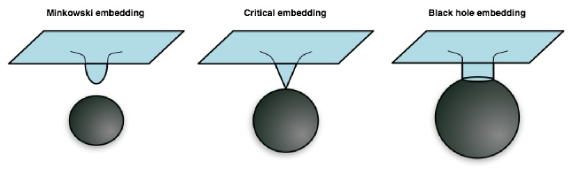
Figure 1: Various Dq-brane configurations in a black Dp-brane background with increasing temperature from left to right. For low temperatures, the probe branes close off smoothly above the horizon. For high temperatures, the branes fall through the event horizon. In between, a critical solution exists in which the branes just ‘touch’ the horizon at a point.

From the viewpoint of the holographic description, the basic physics behind this transition is easily understood. Increasing the temperature increases both the radial position and the energy density of the event horizon in the Dp-brane throat. For a sufficiently small temperature or a sufficiently large separation for the Dq-branes, the probe branes are gravitationally attracted towards the horizon but their tension is sufficient to balance this attractive force. The probe branes then lie entirely outside of the black hole in what we call a ‘Minkowski’ embedding (see fig. 1). However, above a critical temperature $T_{\textrm{\tiny fun}}$, the gravitational force overcomes the tension and the branes are pulled into the horzion. We refer to such configurations where the branes fall through the horizon as ‘black hole’ embeddings. In between these two phases, there exists a critical solution which just ‘touches’ the horizon. In [3], we showed that in the vicinity of this critical solution the embeddings show a self-similar behaviour. As a result, multiple solutions of the embedding equations exist for given temperature in a regime close to $T_{\textrm{\tiny fun}}$. Using thermodynamic considerations to select the true ground state then reveals a first order phase transition at $T_{\textrm{\tiny fun}}$, where the probe branes jump discontinuously from a Minkowski to a black hole embedding.

In the dual field theory, this phase transition is exemplified by discontinuities in, e.g., the quark condensate $\langle\bar{\psi}\psi\rangle$ or the contribution of the fundamental matter to the energy density. However, the most striking feature of this phase transition is found in the spectrum of the mesons, i.e., the quark-antiquark bound states. The latter correspond to excitations supported on the probe branes – see, e.g., [9, 10, 11]. In the low-temperature or Minkowski phase, the mesons are stable (to leading order within the approximations of large $N_{\textrm{\tiny c}}$ and strong coupling) and the spectrum is discrete with a finite mass gap. In the high-temperature or black hole phase, stable mesons cease to exist. Rather one finds a continuous and gapless spectrum of excitations [12, 13]. Hence the first order phase transition is characterised by the dissociation or ‘melting’ of the mesons.

This physics is particularly interesting in theories that exhibit a confinement/deconfinement phase transition. The dual description of the confining, low-temperature phase involves a horizon-free background. At a temperature $T_{\textrm{\tiny deconf}}$ the theory undergoes a phase transition at which the gluons and the adjoint matter become deconfined, at which point the dual background develops a black hole horizon [2]. However, if the mass of the fundamental matter is large enough, the branes remain outside the horizon and therefore mesonic bound states survive for temperatures $T_{\textrm{\tiny deconf}}<T<T_{\textrm{\tiny fun}}$. At $T=T_{\textrm{\tiny fun}}$ the branes finally fall into the horizon, i.e., the mesons melt. This physics is in qualitative agreement with that observed in QCD for heavy-quark mesonic bound states. For example, lattice calculations suggest that charmonium states such as the $J/\psi$ meson melt at temperatures between $1.65T_{\textrm{\tiny deconf}}$ [14, 15] and $2.1T_{\textrm{\tiny deconf}}$ [16], while lattice results for the QCD deconfinement temperature are in the range: $T_{\textrm{\tiny deconf}}\simeq 151$ to $192$ MeV [17]. Although the holographic description may provide some useful geometric intuition for this phenomenon, there are also some caveats that we will discuss in due course.

An overview of the paper is as follows: In section 2, we review the throat geometries for black Dp-branes which are dual to $(p+1)$-dimensional super-Yang-Mills (SYM) at finite temperature [18]. Section 3 reviews and expands on the self-similar behaviour of the embeddings near the critical solution for general Dp/Dq systems, as originally presented in [3]. In the subsequent detailed discussion of the thermodynamics, we focus our attention on the D3/D7 [4] and D4/D6 [5] cases for concreteness. In section 4, we compute the free energy, entropy and energy densities, as well as the speed of sound for the D3/D7 system. We also study the meson spectrum on the Minkowski embeddings in this section. This spectrum is related to the dynamical stability, or lack thereof, of this phase, as we find that tachyonic modes appear where thermodynamic considerations indicate that these embeddings are unstable. Section 5 repeats the salient calculations for the D4/D6 system. Then section 6 concludes with a discussion of results. Finally there are several appendices containing various technical details. Appendix A provides an analytic description of the D7-brane embeddings at very high and very low temperatures. Then appendix B presents some of the details of the calculation of the entropy density contributed by the D7-branes. Appendix C discusses the appearance of the ‘swallow tail’ form in the plots of the free energy, e.g., fig. 5. Appendix D provides a calculation of the constituent quark mass in the low temperature phase of the fundamental matter. Finally, appendix E discusses the holographic renormalization of the D4-brane background.

2 Black Dp-branes

In this section we briefly review the relevant aspects of the throat geometries and thermodynamics of black Dp-branes. This will be of use in subsequent sections, in particular, in sections 4 and 5, where we specialise to black D3- and D4-brane backgrounds, respectively.

2.1 Supergravity Background

The supergravity solution corresponding to the decoupling limit of $N_{\textrm{\tiny c}}$ coincident black Dp-branes is, in the string frame (see, e.g., [19] and references therein),

$$ds^{2} = H^{-\frac{1}{2}}\left(-fdt^{2}+dx_{\it p}^{2}\right)+H^{\frac{1}{2}}\left(\frac{du^{2}}{f}+u^{2}d\Omega_{\it 8-p}^{2}\right)\,,$$

$$e^{\Phi} = H^{\frac{3-p}{4}}\,,\,\,\,\,\,\qquad C_{01\ldots p}=H^{-1}\,,$$ (1)

where $H(u)=(L/u)^{7-p}$ and $f(u)=1-(u_{0}/u)^{7-p}$. The horizon lies at $u=u_{0}$. The length scale $L$ is defined in terms of the string coupling constant $g_{\textrm{\tiny s}}$ and the string length $\ell_{s}$:

$$L^{7-p}=g_{\textrm{\tiny s}}N_{\textrm{\tiny c}}\,(4\pi\ell_{s}^{2})^{\frac{7-p}{2}}\,\Gamma\!\left({\scriptstyle\frac{7-p}{2}}\right)/4\pi\ \,.$$ (2)

For the special case $p=3$, $L$ is the radius of curvature for the AdS${}_{5}\times S^{5}$ geometry appearing in eq. (1).

According to the general gauge/gravity duality of [18], type II string theory in these backgrounds is dual to the super-Yang-Mills $SU(N_{\textrm{\tiny c}})$ gauge theory on the $(p+1)$-dimensional worldvolume of the Dp-branes. For general $p$ ($\neq 3$), the gauge theory is distinguished from the conformal case $(p=3)$ by the fact that the Yang-Mills coupling $g_{\textrm{\tiny YM}}$ is dimensionful. The holographic dictionary provides

$$g_{\textrm{\tiny YM}}^{2}=2\pi g_{\textrm{\tiny s}}(2\pi\ell_{\textrm{\tiny s}})^{p-3}\,.$$ (3)

Hence there is a power-law running of the dimensionless effective coupling with the energy scale $U$:

$$g_{\textrm{\tiny eff}}^{2}={g_{\textrm{\tiny YM}}^{2}N_{\textrm{\tiny c}}}\,U^{p-3}\,,$$ (4)

where $U=u/\alpha^{\prime}$ by virtue of the usual energy/radius correspondence. The absence of conformal invariance for the general case is manifested in the dual geometry by the radial variation of both the string coupling and the spacetime curvature. The supergravity solution (1) is a trustworthy background provided that both the curvatures and string coupling are small. Hence in these general dualities, the supergravity description is limited to an intermediate regime of energies in the field theory or of radial distances in the background. This restriction is succinctly expressed in terms of the effective coupling (4) as [18]:

$$1\ll g_{\textrm{\tiny eff}}\ll N_{\textrm{\tiny c}}^{\frac{4}{7-p}}\,.$$ (5)

Hence the field theory is always strongly coupled where the dual supergravity description is valid.

With the event horizon at $u=u_{0}$, Hawking radiation appears in the background with a temperature fixed by the surface gravity $T=\kappa/2\pi$. This temperature is identified with that of the dual $(p+1)$-dimensional gauge theory. In the geometry (1), the temperature can also be determined by demanding regularity of the Euclidean section obtained through the Wick rotation $t\rightarrow it_{\textrm{\tiny E}}$. Then $t_{\textrm{\tiny E}}$ must be periodically identified with a period $\beta$ where

$$\frac{1}{\beta}=T=\frac{7-p}{4\pi L}\left(\frac{u_{0}}{L}\right)^{\frac{5-p}{2}}\,.$$ (6)

In some cases, one periodically identifies some of the Poincaré directions $x_{\it p}$ in order to render the theory effectively lower-dimensional at low energies; a prototypical example is that of a D4-brane with one compact space direction – see, e.g., [2, 5]. Under these circumstances a different background with no black hole may describe the low-temperature physics, and a phase transition at $T=T_{\textrm{\tiny deconf}}$ may occur [2]. In the gauge theory this is typically a confinement/deconfinement phase transition for the gluonic (or adjoint) degrees of freedom. Throughout this paper we assume that $T>T_{\textrm{\tiny deconf}}$, in which case the appropriate gravitational background has an event horizon, as in eq. (1).

2.2 Thermodynamics

Now as alluded to above, with the Wick rotation $t\rightarrow it_{\textrm{\tiny E}}$, the Euclidean path integral yields a thermal partition function. Further the Euclidean black hole is interpreted as a saddle-point in this path integral and so the gravity action evaluated for this classical solution is interpreted as the leading contribution to the free energy, i.e., $I_{\textrm{\tiny E}}=\beta F$ – see, e.g., [20]. Hence to study the gauge theory thermodynamics holographically, one needs to evaluate the supergravity action $I_{\textrm{\tiny E}}$ for the Euclidean version of the above backgrounds (1). This suffers from IR (large radius) divergences, but these may be regulated by adding appropriate boundary terms to the action. These boundary terms were originally found for asymptotically AdS backgrounds, such as the black D3-brane, in [21, 22]. As we discuss in appendix E, similar surface terms should exist in the general gauge/gravity dualities to complete the holographic description. Here we simply comment that for the black D4-brane, which is the relevant background in section 5, we are guided in the construction of these counterterms by considering the M5-brane counterpart in M-theory. In any event, after including the appropriate boundary terms, the Euclidean action is finite. Then with $F=TI_{\textrm{\tiny E}}$ and standard thermodynamic relations, various thermal quantities can be determined. For example, the entropy $S$ and the energy $E$ are computed as:

$$S=-\frac{\partial F}{\partial T}\,,\,\,\,\,\,\qquad E=F+TS\,.$$ (7)

For the black D3-brane background, the length scale (2) is given by $L^{4}=4\pi g_{s}N_{\textrm{\tiny c}}\ell_{s}^{4}$, and the free energy is

$$F=-\frac{\pi^{6}L^{8}}{16G}\,T^{4}=-\frac{\pi^{2}}{8}N_{\textrm{\tiny c}}^{2}\,T^{4}\,,$$ (8)

where $G$ is the ten-dimensional Newton’s constant. In terms of the string length and coupling, the latter is given by:

$$16\pi G=(2\pi)^{7}\ell_{\textrm{\tiny s}}^{8}\,g_{s}^{2}\,.$$ (9)

For the black D4-brane geometry we have $L^{3}=\pi g_{s}N_{\textrm{\tiny c}}\ell_{s}^{3}$ and

$$F=-\frac{2^{10}\pi^{7}L^{9}}{3^{7}G}\,T^{6}=-\frac{2^{5}\pi^{2}}{3^{7}}\,\lambda\,N_{\textrm{\tiny c}}^{2}\,T^{6}\,,$$ (10)

where as usual $\lambda=g_{\textrm{\tiny YM}}^{2}N_{\textrm{\tiny c}}$ denotes the ’t Hooft coupling. (The reader is referred to appendix E for further discussion of this case.) In general, the free energy for a general black Dp-brane geometry can be written as [18, 23]

$$F\sim N_{\textrm{\tiny c}}^{2}T^{p+1}g_{\textrm{\tiny eff}}(T)^{\frac{2(p-3)}{5-p}}\,,$$ (11)

where

$$g_{\textrm{\tiny eff}}^{2}(T)=\lambda T^{p-3}=g_{\textrm{\tiny YM}}^{2}N_{\textrm{\tiny c}}T^{p-3}$$ (12)

is the effective coupling (4) evaluated at the temperature scale $U=T$. In eq. (11), $N_{\textrm{\tiny c}}^{2}$ reflects the number of degrees of freedom in the $SU(N_{\textrm{\tiny c}})$ gauge theory while $T^{p+1}$ is the expected temperature dependence for a $(p+1)$-dimensional theory. However, the dependence on $g_{\textrm{\tiny eff}}$ is a prediction of the holographic framework for the strongly coupled gauge theory. Note that for the conformal case ($p=3$), but only for this case, this factor is simply unity and so the thermodynamic results can compared to those calculated at weak coupling [24].

Another quantity that is often studied in the context gauge/gravity duality is the speed of sound, e.g., [25, 26, 27, 28, 29]. While this quantity can be inferred from the pole structure of certain correlators [25, 26], it can also be derived from the thermal quantities discussed above, with

$$v_{s}^{2}=\frac{\partial P}{\partial E}=\frac{\partial P}{\partial T}\,\left(\frac{\partial E}{\partial T}\right)^{-1}=\frac{S}{{c_{\textrm{\tiny V}}}}\,.$$ (13)

Here we have used the fact that for a system without a chemical potential, the pressure and free energy density are identical up to a sign, i.e., $P=-F$. Hence $\partial P/\partial T=-\partial F/\partial T=S$. Also we use ${c_{\textrm{\tiny V}}}$ to denote the heat capacity (density), i.e., ${c_{\textrm{\tiny V}}}\equiv\partial E/\partial T$. From eqs. (11) and (12), one finds the simple result that for the strongly coupled gauge theory in $(p+1)$ dimensions

$$v_{s}^{2}=\frac{5-p}{9-p}=\left\{\begin{matrix}\ 1/3&\ \ {\rm for}\ p=3\,,\cr\ 1/5&\ \ {\rm for}\ p=4\,.\cr\end{matrix}\right.$$ (14)

We see above that the conformal result $v_{s}^{2}=1/p$ is only achieved for $p=3$ [25, 26], as expected. We note, however, that the $p=1$ and 4 backgrounds are related through a simple chain of dualities to the AdS₄ and AdS₇ throats of M2- and M5-branes, respectively. Hence for these specific cases with $v_{s}^{2}=1/2$ and 1/5, the speed of sound reflects the conformal nature of the holographic theories dual to these M-theory backgrounds [26].

3 Criticality, scaling, and phase transitions in Dp/Dq systems

We now turn to the systems of interest in this paper: Configurations of probe Dq-branes in the backgrounds of black Dp-branes. The addition of the probes in the gravitational description is dual to the addition of matter in the fundamental representation in the gauge theory [1]. This section is mainly a review of [3] that includes some details that were omitted in that reference. We describe the embedding of the Dq-brane, study the critical behaviour and analyse the nature of the phase transition for general $p$ and $q$. The latter involves extending the Euclidean techniques of the previous section to the worldvolume action of the Dq-brane, to study the thermal properties of the fundamental matter. This discussion naturally leads to sections 4 and 5, where we provide a detailed analysis of the D3/D7 and D4/D6 brane systems.

3.1 Dp/Dq brane intersections

Consider a configuration of $N_{\textrm{\tiny c}}$ coincident black Dp-branes intersecting $N_{\textrm{\tiny f}}$ coincident Dq-branes along $d$ spacelike directions. In the limit $N_{\textrm{\tiny f}}\ll N_{\textrm{\tiny c}}$ the Dq-branes may be treated as a probe in the Dp-brane geometry (1), wrapping an $S^{n}$ inside the $S^{8-p}$. We will assume that the Dq-brane also extends along the radial direction, so that $q=d+n+1$. The corresponding gauge theory now contains fundamental matter propagating along a $(d+1)$-dimensional defect. To ensure stability, we will consider Dp/Dq intersections which are supersymmetric at zero temperature. Generally this means that we are interested in $q=p+4,$ $p+2$ or $p$, as studied in [10, 11]. In this case, the Ramond-Ramond field sourced by the Dp-branes does not couple to the Dq-brane. For the two cases of special interest here, the D3/D7 and the D4/D6 systems, one has $n=3$ and $n=2$ respectively. If the appropriate direction along the D4-brane is compactified, then both cases can effectively be thought of as describing the dynamics of a four-dimensional gauge theory with fundamental matter.

3.2 Critical behaviour

To uncover the critical behaviour of the Dp/Dq brane system, we study the behaviour of the probe brane near the horizon, following [30] closely – see also [31]. First it is useful to adapt the $S^{8-p}$ metric in (1) to the probe brane embedding, and so we write

$$d\Omega_{\it 8-p}^{2}=d\theta^{2}+\sin^{2}\theta\,d\Omega_{\it n}^{2}+\cos^{2}\theta\,d\Omega_{\it 7-p-n}^{2}\,.$$ (15)

As described above, the Dq-brane wraps the internal $S^{n}$ with radius $\sin\theta$ in this line element. Now we zoom in on the near horizon geometry with the coordinates

$$u=u_{0}+\pi Tz^{2}\,,\,\,\,\,\,\theta=\frac{y}{L}\left(\frac{L}{u_{0}}\right)^{\frac{p-3}{4}}\,,\,\,\,\,\,\tilde{x}=\left(\frac{u_{0}}{L}\right)^{\frac{7-p}{4}}x\,,$$ (16)

with $T$ the temperature defined in (6). With these coordinates, the event horizon is at $z=0$. Further $y=0$ denotes the axis running orthogonally to the Dq-brane from the Dp-branes. Expanding the metric (1) to lowest order in $z$ and $y$ gives Rindler space together with some spectator directions:

$$ds^{2}=-(2\pi T)^{2}z^{2}dt^{2}+dz^{2}+dy^{2}+y^{2}d\Omega_{\it n}^{2}+d\tilde{x}_{\it d}^{2}+\cdots\,.$$ (17)

The Dq-brane lies at constant values of the omitted coordinates, so these play no role in the following. The Dq-brane embedding is specified by a curve $(z(\sigma),y(\sigma))$ in the $(z,y)$-plane. Since the dilaton approaches a constant near the horizon, up to an overall constant the Dq-brane (Euclidean) action is simply the volume of the brane, namely

$$I_{\textrm{\tiny bulk}}\propto\int d\sigma\sqrt{\dot{z}^{2}+\dot{y}^{2}}\,zy^{n}\,,$$ (18)

where the dot denotes differentiation with respect to $\sigma$ and the reason for the subscript ‘bulk’ will become clear shortly. This is precisely the action considered in ref. [30]. In the gauge $z=\sigma$ the equation of motion takes the form

$$zy\ddot{y}+(y\dot{y}-nz)(1+\dot{y}^{2})=0\,,$$ (19)

while the gauge choice $y=\sigma$ yields

$$yz\ddot{z}+(nz\dot{z}-y)(1+\dot{z}^{2})=0\,.$$ (20)

The two types of embeddings described in the introduction for the full background extend to this near-horizon geometry (17). Hence the solutions again fall into two classes: ‘black hole’ and ‘Minkowski’ embeddings – see fig. 1. Black hole embeddings are those for which the brane falls into the horizon, and may be characterised by $y_{0}$, the size of the $S^{n}$ there, which is also the size of the induced horizon on the Dq-brane worldvolume. The appropriate boundary condition is $\dot{y}=0,y=y_{0}$ at $z=0$. Minkowski embeddings are those for which the brane closes off smoothly above the horizon. These are characterised by the distance of closest approach to the horizon, $z_{0}$, and satisfy the boundary condition $\dot{z}=0,z=z_{0}$ at $y=0$. There is a simple limiting solution for the equations of motion (19): $y=\sqrt{n}\,z$. This critical solution just touches the horizon at the point $y=z=0$, and so it lies between the above two classes. Note that this point is a singularity in the induced metric of the Dq-brane.

The equation of motion (19) enjoys a scaling symmetry: If $y=f(z)$ is a solution, then so is $y=f(\mu z)/\mu$ for any real positive $\mu$. This transformation rescales $z_{0}\rightarrow z_{0}/\mu$ for Minkowski embeddings, or $y_{0}\rightarrow y_{0}/\mu$ for black hole embeddings, which implies that all solutions of a given type can be generated from any other one by this scaling transformation.

Consider now a solution very close to the critical one, $y(z)=\sqrt{n}\,z+\xi(z)$. Linearising the equation of motion (19), one finds that for large $z$ the solutions are of the form $\xi(z)=z^{\nu_{\pm}}$, with

$$\nu_{\pm}=-\frac{n}{2}\pm\frac{\sqrt{n^{2}-4(n+1)}}{2}\,.$$ (21)

If $n\leq 4$, these exponents have non-vanishing imaginary parts, which leads to oscillatory behaviour. It appears that one can also get real exponents with $n\geq 5$. However, we will show below that no such systems are realized in superstring theory. Hence we will only work with $n\leq 4$ in the following. In this case it is convenient to write the general solution as

$$y=\sqrt{n}\,z+\frac{T^{-1}}{(Tz)^{\frac{n}{2}}}\Big{[}a\sin(\alpha\log Tz)+b\cos(\alpha\log Tz)\Big{]}\,,$$ (22)

where $\alpha=\sqrt{4(n+1)-n^{2}}/2$ and $a,b$ are dimensionless constants determined by $z_{0}$ or $y_{0}$. It is easy to show that under the rescaling discussed above, these constants transform as

$$\begin{pmatrix}a\cr b\end{pmatrix}\rightarrow\frac{1}{\mu^{\frac{n}{2}+1}}\begin{pmatrix}\cos(\alpha\log\mu)&\sin(\alpha\log\mu)\cr-\sin(\alpha\log\mu)&\cos(\alpha\log\mu)\end{pmatrix}\begin{pmatrix}a\cr b\end{pmatrix}\,.$$ (23)

This result implies that the solutions exhibit discrete self-similarity and yields critical exponents that characterise the near-critical behaviour. We refer the reader to [30, 31] for details but emphasise that this behaviour depends only on the dimension of the sphere. Hence it is universal for all Dp/Dq systems (with $n\leq 4$).

Each near-horizon solution gives rise to a global solution when extended over the full spacetime (1). Each of these embeddings is characterised two constants, which can be read off from its asymptotic behaviour and which can be interpreted as the quark mass $M_{\textrm{\tiny q}}$ and (roughly) the quark condensate $\langle\bar{\psi}\psi\rangle$ in the dual field theory – see below. Both of these quantities are fixed by $z_{0}$ or $y_{0}$. As we will see, the values corresponding to the critical solution, $M_{\textrm{\tiny q}}^{*}$ and $\langle\bar{\psi}\psi\rangle^{*}$, give a rough estimate of the point at which a phase transition occurs.

3.2.1 Real scaling exponents?

From eq. (21), we see that the exponents will be real if the dimension of the internal sphere wrapped by the Dq-brane is sufficiently large, i.e., if $n\geq 5$. This would be interesting because, whereas the oscillatory behaviour for $n\leq 4$ leads to a first order phase transition, as we show below, real exponents would seem to lead to a second order phase transition. However, we will now argue that (under the same assumption to guarantee stability as above) no such analysis can be applied for the Dp/Dq systems that actually arise in superstring theory.

Choosing a value of $n$, the dimension of the internal sphere, places restrictions on the allowed values of both $p$ and $q$. The internal $S^{n}$ is a subspace of the spherical part of the geometry (1) and hence we must have $p<8-n$. We have taken a strict inequality here, i.e., we do not consider $p=8-n$, because the size of the $n$-sphere must vary to have nontrivial embeddings and so it can not fill the entire internal (8$-p$)-sphere. Given that $p\geq 0$, we need only consider $n=5,6,7$.

Next, we note that by T-dualising along the $p$ directions common to both sets of branes, the brane configuration is reduced to a D0/D$q^{\prime}$ intersection, where $q^{\prime}=n+1+(p-d)$. Given the previous restriction on $n$, we must have $q^{\prime}\geq 6$. Now, if we require as above that the intersection be supersymmetric at zero temperature (for stability), then we must have $q^{\prime}=8$. Hence the only brane configurations of interest are T-dual to the D0/D8 system. However, these configurations are those in which string creation arises through the Hanany-Witten effect [32]. In particular, as discussed in [33], the background Ramond-Ramond field of the Dp-branes will induce a nontrivial worldvolume gauge field on the Dq-brane. While this does not rule out the possibility of interesting embeddings and a possible (second order) phase transition, it certainly indicates that the present analysis (with no worldvolume gauge fields) does not apply to these systems. For this reason, in the remainder of this paper we will concentrate on Dp/Dq systems with $n\leq 4$.

3.3 Phase Transitions

In order to study the global solutions corresponding to the near horizon solutions of the previous subsection it is convenient to introduce an isotropic, dimensionless radial coordinate $\rho$ through

$$\left(u_{0}\rho\right)^{\frac{7-p}{2}}=u^{\frac{7-p}{2}}+\sqrt{u^{7-p}-u_{0}^{7-p}}\,.$$ (24)

Note that the horizon is at $\rho=1$. Following the discussion in the previous subsection, we assume that the Dp/Dq system under consideration is T-dual to the D3/D7 one, in which case $(p-d)+(n+1)=4$. Then the Euclidean Dq-brane action density of $N_{\textrm{\tiny f}}$ coincident Dq-branes in the black Dp-brane background is

$$\frac{I_{\textrm{\tiny bulk}}}{{\cal N}}=\int_{{\rho_{\textrm{\tiny min}}}}^{\infty}d\rho\left(\frac{u}{u_{0}\rho}\right)^{d-3}\left(1-\frac{1}{\rho^{2(7-p)}}\right)\rho^{n}{(1-\chi^{2})}^{\frac{n-1}{2}}\sqrt{1-\chi^{2}+\rho^{2}\dot{\chi}^{2}}\,,$$ (25)

where $\chi=\cos\theta$, $\dot{\chi}=d\chi/d\rho$ and we have introduced the normalisation constant

$${\cal N}=\frac{N_{\textrm{\tiny f}}T_{\textrm{\tiny Dq}}u_{0}^{n+1}\Omega_{n}}{4T}\,.$$ (26)

Here, $T_{\textrm{\tiny Dq}}=1/{(2\pi\ell_{s})}^{q}g_{s}\ell_{s}$ is the Dq-brane tension and $\Omega_{n}$ is the volume of a unit $n$-sphere. Up to a numerical constant of $O(1)$, the normalisation factor is found to be

$${\cal N}\sim N_{\textrm{\tiny f}}N_{\textrm{\tiny c}}T^{d}g_{\textrm{\tiny eff}}(T)^{\frac{2(d-1)}{5-p}}\,,$$ (27)

where $g_{\textrm{\tiny eff}}(T)$ is the effective coupling (12) and we have used the standard gauge/gravity relations (2) and (3).

The equation of motion that follows from (25) leads to the large-$\rho$ behaviour

$$\chi=\frac{m}{\rho}+\frac{c}{\rho^{n}}+\cdots\,.$$ (28)

Holography relates the dimensionless constants $m,c$ to the quark mass and condensate by

$$M_{\textrm{\tiny q}} = \frac{u_{0}m}{2^{\frac{9-p}{7-p}}\pi\ell_{s}^{2}}\sim g_{\textrm{\tiny eff}}(T)^{\frac{2}{5-p}}\,T\,m\,,$$ (29)

$$\langle{\cal O}_{m}\rangle = -\frac{2\pi\ell_{s}^{2}(n-1)\Omega_{n}N_{\textrm{\tiny f}}T_{\textrm{\tiny Dq}}u_{0}^{n}c}{4^{\frac{n}{7-p}}}\sim-N_{\textrm{\tiny f}}\,N_{\textrm{\tiny c}}\,g_{\textrm{\tiny eff}}^{\frac{2(d-2)}{5-p}}\,T^{d}\,c\,.$$ (30)

Here $M_{\textrm{\tiny q}}$ is the mass of the fields in the fundamental hypermultiplets, both the fermions $\psi$ and the scalars $q$. The operator ${\cal O}_{m}$ is a supersymmetric version of the quark bilinear, and it takes the schematic form

$${\cal O}_{m}=\bar{\psi}\psi+q^{\dagger}\Phi q+M_{\textrm{\tiny q}}q^{\dagger}q\,,$$ (31)

where $\Phi$ is one of the adjoint scalars. We will loosely refer to its expectation value as the ‘quark condensate’. A detailed discussion of this operator, including a precise definition, can be found in appendix A of ref. [35].

Eq. (29) implies the relation $m^{(5-p)/2}=\bar{M}/T$ between the dimensionless quantity $m$, the temperature $T$ and the mass scale

$$\bar{M}=\frac{7-p}{2^{\frac{9-p}{7-p}}\pi L}\left(\frac{2\pi\ell_{s}^{2}M_{\textrm{\tiny q}}}{L}\right)^{\frac{5-p}{2}}\sim\frac{M_{\textrm{\tiny q}}}{g_{\textrm{\tiny eff}}(M_{\textrm{\tiny q}})}\,.$$ (32)

Up to numerical factors, this scale is the mass gap in the discrete meson spectrum at temperatures well below the phase transition [9, 10, 11, 5]. We shall see below that it is also the scale of the temperature of the phase transition for the fundamental degrees of freedom, $T_{\textrm{\tiny fun}}\sim\bar{M}$, since the latter takes place at $m\sim 1$.

The key observation [31] is that the values $(m,c)$ of a near-critical solution are linearly related to the integration constants fixing the corresponding embedding in the near-horizon region. Combining this with the transformation rule (23) for the near-horizon constants $(a,b)$ and eliminating $\mu$, we deduce that $(m-m^{*})/z_{0}^{\frac{n}{2}+1}$ and $(c-c^{*})/z_{0}^{\frac{n}{2}+1}$ are periodic functions of $(\alpha/2\pi)\log z_{0}$ with unit period for Minkowski embeddings, and similarly with $z_{0}$ replaced by $y_{0}$ for black hole embeddings. This is confirmed by our numerical results, which will be discussed in the next sections and are illustrated for the D3/D7 brane system in figure 3.

The oscillatory behaviour of $m$ and $c$ as functions of $z_{0}$ or $y_{0}$ implies that for a fixed value of $m$ near the critical value, several consistent Dq-brane embeddings are possibile with different values of $c$. Alternatively, one finds the quark condensate is not a single-valued function of the quark mass. Physically, the preferred solution will be the one that minimises the free energy density of the Dq-brane, $F=TI_{\textrm{\tiny Dq}}$. As with the bulk action, the Dq-action (25) contains large-radius divergences, as can be seen by substituting the asymptotic behaviour (28) in eq. (25). It therefore needs to be regularised and renormalised. We can achieve the former by replacing the upper limit of integration by a finite ultraviolet cut-off ${\rho_{\textrm{\tiny max}}}$. Then in analogy to the holographic renormalisation of the supergravity action [21, 22], boundary ‘counter-terms’ $I_{\textrm{\tiny bound}}$ are added to the brane action $I_{\textrm{\tiny bulk}}$, such that the renormalised brane energy $I_{\textrm{\tiny Dq}}=I_{\textrm{\tiny bulk}}+I_{\textrm{\tiny bound}}$ is then finite as the cut-off is removed, ${\rho_{\textrm{\tiny max}}}\rightarrow\infty$ [36]. The latter method applies directly to asymptotic AdS geometries, but it can be easily extended to the D4/D6 system, as discussed below. We expect that a similar procedure can be developed for any Dp/Dq system for which there is a consistent gauge/gravity duality. (In any event, the brane action can also be regulated by subtracting the free energy of a fiducial embedding.) The details for the D3/D7 and D4/D6 cases are discussed in the following sections and the results are presented in figures 5 and 12, respectively. In both cases, we see that as the temperature is increased, a first order phase transition occurs by discontinuously jumping from a Minkowski embedding (point A) to a black hole embedding (point B). We emphasise again that this first order transition is a direct consequence of the multi-valued nature of the physical quantities brought on by the critical behaviour described in the previous section. It may be possible to access this self-similar region by super-cooling the system (although most of the other solutions in this region are dynamically unstable – see below).

It is interesting to ask if the strong coupling results obtained here could in principle be compared with a weak coupling calculation. It follows from our analysis that the free energy density takes the form $F={\cal N}Tf(m^{2})$, where the function $f$ can only depend on even powers of $m$ because of the reflection symmetry $\chi\rightarrow-\chi$. The limit $m\rightarrow 0$ may be equivalently regarded as a zero quark mass limit or as a high-temperature limit. In this limit the brane lies near the equatorial embedding $\chi=0$, which slices the horizon in two equal parts. In general $f(0)$ is a non-zero numerical constant; in the D3/D7 case, for example, a straightforward calculation yields $f(0)=-1/2$. Given eq. (27), we have that at strong coupling the free energy density scales as

$$F\sim N_{\textrm{\tiny f}}\,N_{\textrm{\tiny c}}\,T^{d+1}\,g_{\textrm{\tiny eff}}(T)^{\frac{2(d-1)}{5-p}}\,.$$ (33)

The temperature dependence is that expected on dimensional grounds for a $d$-dimensional defect, and the $N_{\textrm{\tiny f}}N_{\textrm{\tiny c}}$ dependence follows from large-$N$ counting rules. However, the dependence on the effective ’t Hooft coupling indicates that this contribution comes as a strong coupling effect, without direct comparison to any weak coupling result. The same is true for other thermodynamic quantities such as, for example, the entropy density $S=-\partial F/\partial T$. We remind the reader that the background geometry makes the leading contribution to the free energy density (11), which corresponds to that coming from the gluons and adjoint matter. Recall that only for $p=3$ is the effective coupling factor absent in eq. (11). Only in this case the string coupling result differs from that at weak coupling by a mere numerical factor of 3/4 [24]. For the fundamental matter, a similar circumstance arises for $d=1$, as would be realized with the D1/D5, D2/D4 or D3/D3 systems. In these special cases, the strong and weak coupling calculations for the fundamental matter could in principle be compared. Hence the D3/D3 system is singled out since such a comparison can be made for both the adjoint and fundamental sectors.

4 The D3/D7 system

Here we will specialise the above discussion to the D3/D7 system. This intersection is summarised by the array

$$\begin{array}[]{ccccccccccc}&0&1&2&3&4&5&6&7&8&9\\ \mbox{D3:}&\times&\times&\times&\times&&&&&&\\ \mbox{D7:}&\times&\times&\times&\times&\times&\times&\times&\times&&\\ \end{array}$$ (34)

Of course, this is an interesting system because both the gluons and the fundamental fields in the gauge theory propagate in $3+1$ dimensions.

4.1 D7-brane embeddings

In the D3/D7 brane system with the radial coordinate defined in (24),

$$(u_{0}\rho)^{2}=u^{2}+\sqrt{u^{4}-u_{0}^{4}}\,,$$ (35)

the background metric (1) becomes

$$ds^{2}=\frac{1}{2}\left(\frac{u_{0}\rho}{L}\right)^{2}\left[-{f^{2}\over\tilde{f}}dt^{2}+\tilde{f}dx^{2}_{3}\right]+\frac{L^{2}}{\rho^{2}}\left[d\rho^{2}+\rho^{2}d\Omega_{5}^{2}\right]\,,$$ (36)

where

$$f(\rho)=1-\frac{1}{\rho^{4}}\,,\,\,\,\,\,\tilde{f}(\rho)=1+\frac{1}{\rho^{4}}\,.$$ (37)

The coordinates $\{t,x^{i}\}$ parametrise the intersection, while $\{\rho,\Omega_{5}\}$ are spherical coordinates on the 456789-directions transverse to the D3-branes. As in eq. (15), it is useful to adapt the metric on the five-sphere to the D7-brane embedding. Since the D7-brane spans the 4567-directions, we introduce spherical coordinates $\{r,\Omega_{3}\}$ in this space and $\{R,\phi\}$ in the 89-directions. Denoting by $\theta$ the angle between these two spaces we then have:

$$\rho^{2}=r^{2}+R^{2}\,,\,\,\,\,\,r=\rho\sin\theta\,,\,\,\,\,\,R=\rho\cos\theta\,,$$ (38)

and

$$d\rho^{2}+\rho^{2}d\Omega^{2}_{5} = d\rho^{2}+\rho^{2}\left(d\theta^{2}+\sin^{2}\theta\,d\Omega^{2}_{3}+\cos^{2}\theta\,d\phi^{2}\right)\,$$ (39)

$$= dr^{2}+r^{2}d\Omega^{2}_{3}+dR^{2}+R^{2}d\phi^{2}\,.$$ (40)

Describing the profile in terms of $\chi(\rho)=\cos\theta(\rho)$ simplifies the analysis – note that $\chi=R/\rho$. With this coordinate choice, the induced metric on the D7-brane becomes

$$ds^{2}=\frac{1}{2}\left(\frac{u_{0}\rho}{L}\right)^{2}\left[-{f^{2}\over\tilde{f}}dt^{2}+\tilde{f}dx_{3}^{2}\right]+\left(\frac{L^{2}}{\rho^{2}}+\frac{L^{2}\dot{\chi}^{2}}{1-\chi^{2}}\right)d\rho^{2}+L^{2}(1-\chi^{2})\,d\Omega_{3}^{2}\,,$$ (41)

where, as above, $\dot{\chi}=d\chi/d\rho$. Since we are studying static embeddings of the probe brane, the equation of motion for $\chi(\rho)$ can be derived equally well from the Lorentzian or Euclidean action. Here we proceed directly to the latter because it is relevant for the thermodynamic calculations in the following. The Euclidean D7-brane action density is

$$\frac{I_{\textrm{\tiny bulk}}}{{\cal N}}=\int d\rho\left(1-\frac{1}{\rho^{8}}\right)\rho^{3}(1-\chi^{2})\sqrt{1-\chi^{2}+\rho^{2}\dot{\chi}^{2}}\,,$$ (42)

where

$${\cal N}=\frac{2\pi^{2}N_{\textrm{\tiny f}}T_{\textrm{\tiny D7}}u_{0}^{4}}{4T}=\frac{\lambda N_{\textrm{\tiny f}}N_{\textrm{\tiny c}}}{32}\,T^{3}$$ (43)

is the normalisation constant defined in (26). Recall from footnote 3 that $I_{\textrm{\tiny bulk}}$ denotes a density because we have divided out the volume $V_{x}$. The equation of motion for $\chi(\rho)$ is then

$$\partial_{\rho}\left[\left(1-\frac{1}{\rho^{8}}\right)\frac{\rho^{5}(1-\chi^{2})\dot{\chi}}{\sqrt{1-\chi^{2}+\rho^{2}\dot{\chi}^{2}}}\right]+\rho^{3}\left(1-\frac{1}{\rho^{8}}\right)\frac{3\chi(1-\chi^{2})+2\rho^{2}\chi\dot{\chi}^{2}}{\sqrt{1-\chi^{2}+\rho^{2}\dot{\chi}^{2}}}=0\,,$$ (44)

which implies that the field $\chi$ asymptotically approaches zero as

$$\chi=\frac{m}{\rho}+\frac{c}{\rho^{3}}+\cdots\,.$$ (45)

The dimensionless constants $m$ and $c$ are related to the quark mass and condensate through eqs. (29) and (30) with $p=3$ and $n=3$:

$$M_{\textrm{\tiny q}} = \frac{u_{0}m}{2^{3/2}\pi\ell_{s}^{2}}=\frac{1}{2}\sqrt{\lambda}\,T\,m\,,$$ (46)

$$\langle{\cal O}_{m}\rangle = -2^{3/2}\pi^{3}\ell_{s}^{2}N_{\textrm{\tiny f}}T_{\textrm{\tiny D7}}u_{0}^{3}\,c=-\frac{1}{8}\sqrt{\lambda}\,N_{\textrm{\tiny f}}\,N_{\textrm{\tiny c}}\,T^{3}\,c\,.$$ (47)

In this case $m=\bar{M}/T$ and eq. (32) takes the form

$$\bar{M}=\frac{\sqrt{2}(2\pi\ell_{s}^{2}M_{\textrm{\tiny q}})}{\pi L^{2}}=\frac{2M_{\textrm{\tiny q}}}{\sqrt{\lambda}}=\frac{M_{\textrm{\tiny gap}}}{2\pi}\,,$$ (48)

where $\lambda=g_{\textrm{\tiny YM}}^{2}N_{\textrm{\tiny c}}=2\pi g_{s}N_{\textrm{\tiny c}}$ is the ’t Hooft coupling. In the last equality, we are relating $\bar{M}$ to the meson mass gap in the D3/D7 theory at zero temperature [9].

The equation of motion (44) can be recast in terms of the $R$ and $r$ coordinates, related to the $\rho$ and $\theta$ coordinates via (38):

$$\partial_{r}\left[r^{3}\left(1-{1\over(r^{2}+R^{2})^{4}}\right){\partial_{r}R\over\sqrt{1+(\partial_{r}R)^{2}}}\right]=8{r^{3}R\over(r^{2}+R^{2})^{5}}\sqrt{1+(\partial_{r}R)^{2}}\,,$$ (49)

where the embedding of the D7-brane is now specified by $R=R(r)$. Asymptotically,

$$R(r)=m+\frac{c}{r^{2}}+\cdots\,.$$ (50)

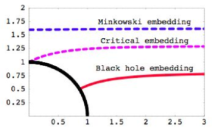
Figure 2: Profiles various D7-brane embeddings in a D3-brane background in the $(R,r)$-plane. The circle represents the horizon at $\rho=1$.

In the limits of large and small $m$ we were able to find approximate analytic solutions for the embeddings – see discussion below and Appendix A. However, for arbitrary $m$ we were unable to find an analytic solution of eq. (44) or (49) and so we resorted to solving these equations numerically. It was simplest to solve for Minkowski embeddings using the $(R,r)$ coordinates with equation of motion (49) while the $(\chi,\rho)$ coordinates were best suited to the black hole embeddings. Our approach was to specify the boundary conditions at a minimum radius and then numerically integrate outward. For the black hole embeddings, the following boundary conditions were specified at the horizon ${\rho_{\textrm{\tiny min}}}=1$: $\chi=\chi_{0}$ and $d\chi/d\rho=0$ for $0\leq\chi_{0}<1$. For Minkowski embeddings, the following boundary conditions were specified at $r_{min}=0$ (i.e., at the axis $\chi=1$): $R=R_{0}$ and $\partial_{r}R=0$ for $R_{0}>1$. In order to compute the constants $m,c$ corresponding to each choice of boundary conditions at the horizon, we fitted the solutions to the asymptotic form (45) for $\chi(\rho)$ or (50) for $R(r)$. A few characteristic profiles are shown in fig. 2.

Recall that, as elucidated in section 3.2, the black hole and Minkowski embeddings are separated by a critical solution which just touches the horizon. This critical embedding is characterised by certain critical values of the integration constants, $m^{\ast}$ and $c^{\ast}$. For Minkowski embeddings near the critical solution, fig. 3 shows plots of $(m-m^{\ast})/(R_{0}-1)^{5/2}$ and $(c-c^{\ast})/(R_{0}-1)^{5/2}$ versus $\sqrt{7}\log(R_{0}-1)/4\pi$. In this regime, we may relate the boundary value to that in the near horizon analysis with $R_{0}-1\simeq z_{0}$. Here our numerical results confirm that, near the critical solution, $(m-m^{\ast})/z_{0}^{5/2}$ and $(c-c^{\ast})/z_{0}^{5/2}$ are both periodic functions of $\sqrt{7}\log(z_{0})/4\pi$ with unit period, as discussed above in section 3.2. This oscillatory behaviour of $m$ and $c$ as functions of $z_{0}$ (or $y_{0}$) implies that the quark condensate is not a single-valued function of the quark mass and this is clearly visible in our plots of $c$ versus $T/\bar{M}=1/m$, displayed in figure 4. By increasing the resolution in these plots, we are able to follow the two families of embeddings spiralling in on the critical solution, the behaviour predicted by the near-horizon analysis. Thermodynamic considerations will resolve the observed multi-valuedness by determining the physical solution as that which minimizes the free energy density of the D7-branes. As discussed in section 3.3, since the physical parameters are multi-valued, we can anticipate that there will be a first order phase transition when the physical embedding moves from the Minkowski branch to the black hole branch. We will proceed to computing the free energy density in the next subsection. The position of the resulting phase transition is indicated in the second plot of fig. 4.

Figure 3: Quark mass (a) and condensate (b) as a function of the distance to the horizon $R_{0}-1$ for D7-brane Minkowski embeddings in a D3-brane background. Note that near the horizon $R_{0}-1\sim z_{0}$.

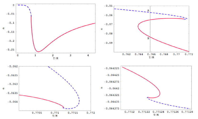
Figure 4: Quark condensate $c$ for a D7 in a D3 background versus $T/\bar{M}$. The blue dashed (red continuous) curves correspond to the Minkowski (black hole) embeddings. The dotted vertical line indicates the precise temperature of the phase transition.

4.2 D7-brane thermodynamics

Having discussed the embeddings of the D7-brane in the black D3-brane geometry, we proceed to compute the free energy, entropy and energy densities associated with the D7-brane, or equivalently, the fundamental fields. We start with the Euclidean D7-brane action (42). Using the asymptotic behaviour (45), we see that the action contains a UV divergence, since

$$\frac{I_{\textrm{\tiny bulk}}}{{\cal N}}\simeq\int_{{\rho_{\textrm{\tiny min}}}}^{{\rho_{\textrm{\tiny max}}}}d\rho\,\rho^{3}\simeq\frac{1}{4}{\rho_{\textrm{\tiny max}}}^{4}$$ (51)

diverges as the regulator is removed, i.e., ${\rho_{\textrm{\tiny max}}}\to\infty$.

This kind of problem is well-known in the context of the AdS/CFT correspondence and was first resolved for the gravity action by introducing boundary counter-terms, which depend only on the intrinsic geometry of the boundary metric [21, 22]. These ideas can be generalized to other fields in an AdS background, such as a scalar [37] – for a review, see [38]. The latter formed the basis for the renormalization of probe brane actions in [36], where the brane position or profile is treated as a scalar field in an asymptotically AdS geometry. That is, one implicitly performs a Kaluza-Klein reduction of the D7 action to five dimensions so that it appears to be a complicated nonlinear action for a scalar field $\chi$ propagating in a five-dimensional (asymptotically) AdS geometry. One then introduces boundary counter-terms which are local functionals (polynomials) of the scalar field (and boundary geometry) on an asymptotic regulator surface. These terms are designed to remove the bulk action divergences that arise as the regulator surface is taken off to infinity, as in eq. (51). The D3/D7 system is explicitly considered in ref. [36], which also introduces a finite counterterm that ensures that the brane action vanishes for the supersymmetric embedding of a D7-brane in an extremal D3-background, i.e., eq. (1) with $u_{0}=0$ and $p=3$. In the calculation of [36] the D7-brane embedding is specified as $\theta(\rho)$, but this is easily converted to a counter-term action for $\chi(\rho)$ using the obvious coordinate/field redefinition: $\frac{\pi}{2}-\theta=\arcsin\chi\simeq\chi+1/6\,\chi^{3}+\cdots$. The final result is

$${I_{\textrm{\tiny bound}}\over{\cal N}}=-{L^{4}T\over u_{0}^{4}}\int dt_{\textrm{\tiny E}}d^{3}x\sqrt{\det\gamma}\left(1-2\chi^{2}+\chi^{4}\right)\,,$$ (52)

where this boundary action is evaluated on the asymptotic regulator surface $\rho={\rho_{\textrm{\tiny max}}}$ introduced above. The boundary metric $\gamma$ at $\rho={\rho_{\textrm{\tiny max}}}$ in the (effective) five-dimensional geometry is given by

$$ds^{2}(\gamma)={1\over 2}\left({u_{0}{\rho_{\textrm{\tiny max}}}\over L}\right)^{2}\left({f({\rho_{\textrm{\tiny max}}})^{2}\over\tilde{f}({\rho_{\textrm{\tiny max}}})}\,dt_{\textrm{\tiny E}}^{2}+\tilde{f}({\rho_{\textrm{\tiny max}}})dx_{3}^{\,2}\right)$$ (53)

and so $\sqrt{\gamma}={u_{0}^{4}{\rho_{\textrm{\tiny max}}}^{4}}f({\rho_{\textrm{\tiny max}}})\tilde{f}({\rho_{\textrm{\tiny max}}})/4L^{4}$. Evaluating the counter-term action (52) with an asymptotic profile as in eq. (28), one finds

$${I_{\textrm{\tiny bound}}\over{\cal N}}=-{1\over 4}\left[({\rho_{\textrm{\tiny max}}}^{2}-m^{2})^{2}-4mc\right].$$ (54)

Here we have divided out the volume factor $V_{x}$ – see footnote 3. Comparing eqs. (51) and (54), one sees that the leading divergence proportional to $\rho^{4}_{\textrm{\tiny max}}$ cancels in the sum of $I_{\textrm{\tiny D7}}=I_{\textrm{\tiny bulk}}+I_{\textrm{\tiny bound}}$. As a further check, one can consider the supersymmetric limit $u_{0}\rightarrow 0$, in which one must work with a rescaled coordinate $\tilde{\rho}=u_{0}\rho$, since the change of variables (35) is not well defined at $u_{0}=0$. In this limit $\chi=u_{0}m/\tilde{\rho}=\sqrt{2}\,2\pi\ell_{s}^{2}M_{\textrm{\tiny q}}/\tilde{\rho}$ is an exact solution, and one can easily verify that for this configuration $I_{\textrm{\tiny D7}}=I_{\textrm{\tiny bulk}}+I_{\textrm{\tiny bound}}=0$.

In order to produce a finite integral which is more easily evaluated numerically, it is useful to incorporate the divergent terms in the boundary action (54) into the integral in eq. (42) using

$${\rho_{\textrm{\tiny max}}}^{4} = \int_{{\rho_{\textrm{\tiny min}}}}^{{\rho_{\textrm{\tiny max}}}}d\rho\,4\rho^{3}+{\rho_{\textrm{\tiny min}}}^{4}\ ,$$

$${\rho_{\textrm{\tiny max}}}^{2} = \int_{{\rho_{\textrm{\tiny min}}}}^{{\rho_{\textrm{\tiny max}}}}d\rho\,2\rho+{\rho_{\textrm{\tiny min}}}^{2}\ .$$ (55)

Then the total action may be written as

$${I_{\textrm{\tiny D7}}\over{\cal N}}=G(m)-{1\over 4}\left[({\rho_{\textrm{\tiny min}}}^{2}-m^{2})^{2}-4mc\right]\ ,$$ (56)

where $G(m)$ is defined as

$$G(m)=\int_{{\rho_{\textrm{\tiny min}}}}^{\infty}d\rho\,\left[\rho^{3}\left(1-{1\over\rho^{8}}\right)\left(1-\chi^{2}\right)\left(1-\chi^{2}+\rho^{2}\,\dot{\chi}^{2}\right)^{1/2}-\rho^{3}+m^{2}\rho\right].$$ (57)

Note that the upper bound for the range of integration has been set to infinity, since the integral above is finite.

From these expressions, the free energy density is given by $F=TI_{D7}$. Now using our numerical results, the free energy density is shown as a function of the temperature in the first two plots in fig. 5. The second of these shows the classic ‘swallow tail’ form, typically associated with a first order phase transition. To our best numerical accuracy, the phase transition takes place at $T_{\textrm{\tiny fun}}/\bar{M}=0.7658$ (or $m=1.306$), where the free energy curves for the Minkowski and black hole phases cross. The fact that the transition is first order is illustrated by fig. 4, which shows that the quark condensate makes a finite jump at this temperature between the points labelled A and B. Similar discontinuities also appear in other physical quantities, like the entropy and energy density, as we now calculate.

Given the free energy density, a standard identity (7) yields the entropy density as

$$S=-\frac{\partial F}{\partial T}=-\pi L^{2}\frac{\partial F}{\partial u_{0}}\,,$$ (58)

where we have used the expression $u_{0}=\pi L^{2}T$ from eq. (6). Evaluating this expression requires a straightforward but somewhat lengthy calculation, which we have relegated to appendix B. The final result is

$${S\over{\cal N}}=-4G(m)+({\rho_{\textrm{\tiny min}}}^{2}-m^{2})^{2}-6mc\,.$$ (59)

Comparing eqs. (56) and (59), we see that the entropy and free energy densities are simply related as

$$S=-\frac{4F}{T}\left(1+\frac{2\,{\cal N}\,mc}{4F/T}\right)\,.$$ (60)

The first term above can be recognized as the behaviour expected for a conformal system, i.e., a system for which $F\propto T^{4}$. Hence the second term can be interpreted as summarising the deviation from conformal behaviour. We note that, as illustrated in fig. 4, $c$ vanishes in both the limits $T\rightarrow 0$ and $T\rightarrow\infty$ and so the deviation from conformality is reduced there. More precisely, using the results from appendix A we see that $c\sim m$ at high temperature and $c\sim 1/m^{5}$ at low temperature. Together with (43) this implies that the deviation from conformality scales as $\bar{M}^{2}/T^{2}$ at high temperature. Conformality is also restored at low temperatures but only because both $S$ and $F/T$ approach zero more quickly than $T^{3}$. That is, $S\sim T^{7}/\bar{M}^{4}$ as $T\rightarrow 0$.

Finally, the thermodynamic identity $E=F+TS=T(I_{\textrm{\tiny D7}}+S)$ gives the contribution of the D7-brane to the energy density:

$${E\over{\cal N}T}=-3G(m)+{3\over 4}\left[({\rho_{\textrm{\tiny min}}}^{2}-m^{2})^{2}-{20\over 3}mc\right].$$ (61)

We evaluated both the expressions (59) and (61) numerically and plotted $S$ and $E$ in fig. 5. In both cases, the phase transition is characterised by a finite jump in these quantities, as illustrated by the second plot in each case. However, these plots also show that there is a large rise in, say, the entropy density in the vicinity of $T_{\textrm{\tiny fun}}$ and that the jump associated with the phase transition only accounts for roughly $3\%$ of this total increase.

We close with a few observations about these results. First, recall from (43) that ${\cal N}\sim\lambda N_{\textrm{\tiny c}}N_{\textrm{\tiny f}}T^{3}$ so that the leading contribution of the D7-branes to all the various thermodynamic quantities will be order $\lambda N_{\textrm{\tiny c}}N_{\textrm{\tiny f}}$, in comparison to $N_{\textrm{\tiny c}}^{2}$ for the usual bulk gravitational contributions. As noted in [3, 34], the factor of $\lambda$ represents a strong coupling enhancement over the contribution over a simple free-field estimate for the $N_{\textrm{\tiny c}}N_{\textrm{\tiny f}}$ fundamental degrees of freedom. We return to this point below in section 6.

Next, note that in order for the entropy $S=-\partial F/\partial T$ to be positive, the free energy $F$, or equivalently the action $I_{\textrm{\tiny D7}}$, must always be a decreasing function of the temperature. This means that the apparent ‘kinks’ in the plot of these quantities versus the temperature are true mathematical kinks and not just very rapid turn overs. An analytic proof of this fact is given in appendix C.

Finally, from the plots of the energy density one can immediately read off the qualitative behaviour of the specific heat $c_{V}=\partial E/\partial T$. In particular, note that this slope must become negative as the curves spiral around near the critical solution. Hence the corresponding embeddings are thermodynamically unstable. Examining the fluctuation spectrum of the branes, we will show that a corresponding dynamical instability sets in at precisely the same points. One may have thought that these phases near the critical point could be accessed by ‘super-cooling’ the system but this instability severely limits the embeddings which can be reached with such a process.

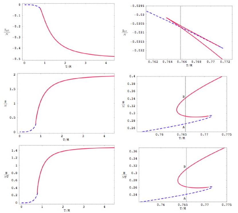
Figure 5: Free-energy, entropy and energy densities for a D7-brane in a D3-brane background; note that ${\cal N}\propto T^{3}$. The blue dashed (red continuous) curves correspond to the Minkowski (black hole) embeddings. The dotted vertical line indicates the precise temperature of the phase transition.

4.2.1 Thermodynamic expressions for large $T/\bar{M}$

With precisely $m=0$, $\chi(\rho)=0$ is an exact solution. We denote this solution as the equatorial embedding, since the D7-brane remains at the maximal $S^{3}$ for all values of $\rho$. This embedding describes the infinite-temperature limit for massive quarks (or massless quarks for any temperature), i.e., $T/\bar{M}\rightarrow\infty$. For $T/\bar{M}\gg 1$ or $m\ll 1$, approximate analytic solutions for the D7-brane profile can be found by perturbing around the equatorial embedding, as discussed in appendix A. The final result is given in eq. (126). In the notation of the appendix, the integral (57) can be expressed as

$$G(m) = \int_{1}^{\infty}{dx\over 2}\left[x\left(1-{1\over x^{4}}\right)\left(1-{3\over 2}m^{2}\tilde{\chi}^{2}+2x^{2}\left(\partial_{x}m\tilde{\chi}\right)^{2}\right)-x+m^{2}\right]$$

$$= -{1\over 4}+m^{2}G_{2}$$

where we have introduced

$$G_{2}\equiv\int_{1}^{\infty}{dx\over 2}\left[x\left(1-{1\over x^{4}}\right)\left(-{3\over 2}\tilde{\chi}^{2}+2x^{2}\left(\partial_{x}\tilde{\chi}\right)^{2}\right)+1\right]\simeq 0.413893\,.$$ (62)

We were only able to evaluate this integral numerically.

We are now in a position to evaluate the various thermal quantities given by eqs. (56), (59) and (61) in this limit. We find

$${I_{\textrm{\tiny D7}}\over{\cal N}} \simeq -{1\over 2}+\left(G_{2}+\tilde{c}+{1\over 2}\right)\left({\bar{M}\over T}\right)^{2}-{1\over 4}\left({\bar{M}\over T}\right)^{4}+\cdots\,,$$

$${S\over{\cal N}} \simeq 2+\left(-4G_{2}-6\tilde{c}-2\right)\left({\bar{M}\over T}\right)^{2}+\left({\bar{M}\over T}\right)^{4}+\cdots\,,$$

$${E\over{\cal N}T} \simeq {3\over 2}+\left(-3G_{2}-5\tilde{c}-{3\over 2}\right)\left({\bar{M}\over T}\right)^{2}+{3\over 4}\left({\bar{M}\over T}\right)^{4}+\cdots\,,$$

using ${\rho_{\textrm{\tiny min}}}=1$ for black hole embeddings and $\tilde{c}\simeq-0.456947$ from eq. (129). In this high temperature limit, the quark mass is negligible and so the first term in these expressions could be characterised as conformal behaviour. The remaining contributions are small corrections indicating a deviation from this simple behaviour generated by the finite quark mass. This is essentially the form expected in the high $T$ limit in finite temperature field theory – for example, see [39] and the references therein.

4.2.2 Thermodynamic expressions for small $T/\bar{M}$

Turning to the opposite, low-temperature limit, i.e., $T/\bar{M}\ll 1$, the D7-branes lie on flat embeddings far from the event horizon, i.e., $\chi\simeq R_{0}/\rho$ to leading order. One can calculate perturbative improvements to this simple embedding – see appendix A – but it suffices to determine the leading thermodynamic behaviour. We find that

$$G(m)=\int_{0}^{\infty}dr\left[r^{3}\left(1-\frac{1}{\rho^{8}}\right)\sqrt{1+\left(\partial_{r}R\right)^{2}}+(r+R\,\partial_{r}R)(m^{2}-\rho^{2})\right]\simeq\frac{1}{12}\frac{1}{m^{4}}\,.\\$$ (63)

Then using $R_{0}\simeq m$ and $c\simeq-1/6m^{5}$, the thermal densities become

$${I_{\textrm{\tiny D7}}\over{\cal N}}\simeq-{1\over 12}\left({T\over\bar{M}}\right)^{4}\,,\qquad{S\over{\cal N}}\simeq\frac{2}{3}\left({T\over\bar{M}}\right)^{4}\,,\qquad{E\over{\cal N}T}\simeq\frac{7}{12}\left({T\over\bar{M}}\right)^{4}\,.$$ (64)

Hence these contributions are going rapidly to zero. Note that they still contain the same normalization constant (43) and so these densities are still proportional to $\lambda N_{\textrm{\tiny f}}N_{\textrm{\tiny c}}$. At low temperature, one might have expected that the thermodynamics of the fundamental matter is dominated by the low lying-mesons, i.e., the lowest energy excitations in the fundamental sector, and so that the leading contributions are proportional to $N_{\textrm{\tiny f}}^{2}$, reflecting the number of mesonic degrees of freedom. Such contributions to the thermal densities will arise in the gravity path integral in evaluating the fluctuation determinant on the D7-brane around the classical saddle-point. As indicated by the $N_{\textrm{\tiny c}}$ and $\lambda$ factors, the leading low-temperature contributions above come from the interaction of the (deconfined) adjoint fields and the fundamental matter.

4.2.3 Speed of sound

As mentioned in section 2.2, the speed of sound is another interesting probe of the deconfined phase of the strongly coupled gauge theories. In this section, we calculate the effect of fundamental matter on the speed of sound. From eq. (13), we must evaluate the D7-branes contribution to the total entropy density and the specific heat. The first is already given by eq. (59) and we denote this contribution as $S_{7}$ in the following. From eq. (61), the energy density can be written as $E=-3F-2{\cal N}Tmc$. Then recalling ${\cal N}\propto T^{3}$ from eq. (43), the D7-brane contribution to the specific heat can be written as

$${c_{\textrm{\tiny V}}}_{7}=\frac{\partial E}{\partial T}=3S_{7}-\alpha\,\frac{\partial}{\partial T}\,(T^{4}\,mc)\,,$$ (65)

where we have introduced the dimensionless constant $\alpha\equiv\lambda N_{\textrm{\tiny f}}N_{\textrm{\tiny c}}/16$. From the black D3 background, the free energy of the adjoint fields is given in eq. (8). It follows then that the adjoint contributions to the entropy and specific heat are:

$$S_{3}=-{\pi^{2}\over 2}N_{\textrm{\tiny c}}^{2}\,T^{3}\,,\qquad{c_{\textrm{\tiny V}}}_{3}=3\,S_{3}\,.$$ (66)

Combining all of these results, we can now calculate the speed of sound

$$v_{s}^{2} = {S\over{c_{\textrm{\tiny V}}}}={S_{3}+S_{7}\over{c_{\textrm{\tiny V}}}_{3}+{c_{\textrm{\tiny V}}}_{7}}$$ (67)

$$= {S_{3}+S_{7}\over 3S_{3}+3S_{7}-\alpha\,\partial_{T}\!\left(T^{4}\,mc\right)}$$

$$\simeq {1\over 3}\left[1+{\alpha\over 3\,S_{3}}\,\partial_{T}\!\left(\,T^{4}\,mc\,\right)\right]\,.$$

Note all of our brane calculations are to first-order in an expansion in $N_{\textrm{\tiny f}}/N_{\textrm{\tiny c}}$ and hence we have applied the Taylor expansion in the last line above, reflecting this perturbative framework e.g., ${c_{\textrm{\tiny V}}}_{7}/{c_{\textrm{\tiny V}}}_{3}\ll 1$. Now using various expressions above, as well as $m=2M_{q}/\sqrt{\lambda}T$ and $\varepsilon\equiv{\lambda\over 2\pi}{N_{\textrm{\tiny f}}\over N_{\textrm{\tiny c}}}$, we may write the final result as

$$\delta v_{s}^{2}\equiv v_{s}^{2}-{1\over 3}\simeq{\varepsilon\over 12\pi}\left(mc+{1\over 3}mT{\partial c\over\partial T}\right)\,.$$ (68)

This expression indicates that the D7-brane produces a small deviation away from the conformal result, $v_{s}^{2}={1\over 3}$.

The result of numerically evaluating $\delta v_{s}^{2}$ as a function of the temperature is given in fig. 6. We see that $\delta v_{s}^{2}$ is negative. That is, the fundamental matter reduces the speed of sound. Following the discussion below eq. (60) one finds that $\delta v_{s}^{2}\sim T^{4}/\bar{M}^{4}$ at low temperature and $\delta v_{s}^{2}\sim\bar{M}^{2}/T^{2}$ at high temperature. Thus we see again that the deviation from conformal behaviour vanishes for large and small $T$. We also note that $\delta v_{s}^{2}$ is largest near the phase transition, where it makes a discrete jump. Since we are working in a perturbative framework, eq. (68) is only valid when this deviation is a small perturbation. By assumption $\varepsilon\propto N_{\textrm{\tiny f}}/N_{\textrm{\tiny c}}\ll 1$ and so this is guaranteed provided the last factor in (68) is not large. This is indeed satisfied for the thermodynamically favoured embeddings, as illustrated in fig. 6. Similar deviations have been investigated in [28] for other gauge/gravity dualities.

In fig. 6, we have also continued $\delta v_{s}^{2}$ on the disfavoured embeddings beyond the phase transition and we see that it diverges (towards $-\infty$) at precisely the points where, e.g., the energy density curve turns around – see fig. 5. That is, ${c_{\textrm{\tiny V}}}_{7}$ diverges at these points, so that the perturbative derivation of eq. (68) breaks down. Hence our perturbative framework does not allow us to investigate interesting effects, as seen in [29].

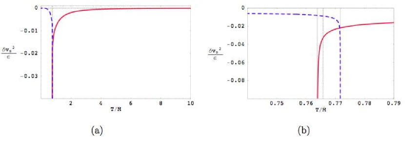
Figure 6: The deviation of the speed of sound from the conformal value. (a) In the limits $T\to 0$ and $T\to\infty$, $\delta v_{s}^{2}\to 0$. (b) The temperature of the phase transition is marked by the dashed vertical line. Note there is a finite discontinuity in the speed of sound at the phase transition. If we follow the black hole branch (red line) or the Minkowski branch (dotted blue line) past the phase transition, we find that $\delta v_{s}^{2}$ diverges.

We see from eq. (68) that, for massive quarks, the deviation from the conformal result is of proportional to $N_{\textrm{\tiny f}}/N_{\textrm{\tiny c}}$, as expected from large-$N_{\textrm{\tiny c}}$ counting rules. However, if $M_{\textrm{\tiny q}}=0$ then the result above vanishes, and so $\delta v_{s}^{2}=O(N_{\textrm{\tiny f}}^{2}/N_{\textrm{\tiny c}}^{2})$ at least. Presumably, this additional suppression is due to the fact that for massive quarks conformal invariance is broken explicitly at the classical level, whereas if $M_{\textrm{\tiny q}}=0$ it is broken only at the quantum mechanical level by the non-vanishing beta function of the theory in the presence of fundamental matter. This is proportional to $N_{\textrm{\tiny f}}/N_{\textrm{\tiny c}}$, leading to an additional suppression. In the gravitational description this is most easily understood at zero temperature. In this case the D3-brane background is exactly $AdS_{5}\times S^{5}$, and the isometries of the first factor correspond to the conformal group in four dimensions. Adding D7-brane probes with non-zero quark mass breaks the conformal isometries, and hence this effect is visible at order $N_{\textrm{\tiny f}}/N_{\textrm{\tiny c}}$. Instead, if $M_{\textrm{\tiny q}}=0$ then the branes’ worldvolume is $AdS_{5}\times S^{3}$, which preserves all the $AdS$ isometries. Hence in this case one must go beyond the probe approximation to see the breaking of conformal invariance, i.e., beyond $O(N_{\textrm{\tiny f}}/N_{\textrm{\tiny c}})$.

4.3 Meson spectrum

As discussed earlier, introducing the D7-brane probes into the black D3-brane geometry corresponds to adding dynamical quarks into the gauge theory. The resulting theory has a rich spectrum of mesons, i.e., quark-antiquark bound states. Since the mesons are dual to open strings with both ends on the D7-brane, the mesonic spectrum can be found by computing the spectrum of D7-brane fluctuations. For temperatures below the phase transition, $T<T_{\textrm{\tiny fun}}$, corresponding to Minkowski embeddings of the D7-branes, we expect the spectrum to exhibit a mass gap and be discrete, just as found at $T=0$ [9, 10, 11]; this is confirmed by our calculations below – similar calculations have also appeared recently in [12]. For temperatures above the phase transition, corresponding to black hole embeddings, the spectrum will be continuous and gapless. Excitations of the fundamental fields in this phase are however characterised by a discrete spectrum of quasinormal modes, in analogy with [40]. Investigations of the black hole phase appear elsewhere [12, 13].

4.3.1 Mesons on Minkowski embeddings

In this section we compute the spectrum of low-lying mesons corresponding to fluctuations of the D7-brane in the black D3-brane geometry (36). The full meson spectrum would include scalar, vector and spinor modes. For simplicity, we will only focus on scalar modes corresponding to geometric fluctuations of the brane about the embeddings determined in section 4.1. We will work with the $(R,r)$ coordinates introduced in eq. (38), in which case the background embedding is given by $R=R_{v}(r)$, $\phi=0$, where the subscript $v$ now indicates that this is the ‘vacuum’ solution. Explicitly, we consider small fluctuations $\delta R,\delta\phi$ about the background embedding:

$$R=R_{v}(r)+\delta R\,,\quad\phi=0+\delta\phi.$$ (69)

The pullback of the bulk metric (36) to this embedding is

$$ds^{2} = \frac{1}{2}\left(\frac{u_{0}\rho}{L}\right)^{2}\left[-{f^{2}\over\tilde{f}}dt^{2}+\tilde{f}dx_{3}^{2}\right]+\frac{L^{2}}{\rho^{2}}\left[(1+\dot{R}_{v}^{2})dr^{2}+r^{2}d\Omega_{3}^{2}+2(\partial_{a}\delta R)\dot{R_{v}}dx^{a}dr\right]$$

$$+\frac{L^{2}}{\rho^{2}}\left[(\partial_{a}\delta R)(\partial_{b}\delta R)dx^{a}dx^{b}+(R_{v}+\delta R)^{2}(\partial_{a}\delta\phi)(\partial_{b}\delta\phi)dx^{a}dx^{b}\right]\,,$$

where the indices $a,b$ run over all D7 worldvolume directions. Using the DBI action, the D7-brane Lagrangian density to quadratic order in the fluctuations is

$$\mathcal{L} = \mathcal{L}_{0}-T_{\textrm{\tiny D7}}\frac{u_{0}^{4}}{4}r^{3}\sqrt{h}\sqrt{1+\dot{R}_{v}^{2}}\left\{\frac{1}{2}\frac{L^{2}}{\rho_{v}^{2}}\left(1-\frac{1}{\rho_{v}^{8}}\right)\sum_{a}g^{aa}\left(\frac{(\partial_{a}\delta R)^{2}}{1+\dot{R}_{v}^{2}}+R_{v}^{2}(\partial_{a}\delta\phi)^{2}\right)\right.$$ (70)

$$+\left.\frac{4R_{v}\dot{R}_{v}\partial_{r}(\delta R)^{2}}{\rho_{v}^{10}(1+\dot{R}_{v}^{2})}+\frac{4(\delta R)^{2}}{\rho_{v}^{10}}-\frac{40R_{v}^{2}(\delta R)^{2}}{\rho_{v}^{12}}\right\}\,,$$

where $\mathcal{L}_{0}$ is the Lagrangian density for the vacuum embedding:

$$\mathcal{L}_{0}=-T_{\textrm{\tiny D7}}\frac{u_{0}^{4}}{4}r^{3}\sqrt{h}\sqrt{1+\dot{R}_{v}^{2}}\left(1-\frac{1}{\rho_{v}^{8}}\right).$$ (71)

Here $\rho_{v}^{2}=r^{2}+R_{v}^{2}$ and $h$ is the determinant of the metric on the $S^{3}$ of unit radius. The metric $g_{ab}$ in the first line of (70) is the induced metric on the D7-brane with the fluctuations set to zero:

$$ds^{2}(g)=\frac{1}{2}\left(\frac{u_{0}\rho_{v}}{L}\right)^{2}\left[-{f^{2}\over\tilde{f}}dt^{2}+\tilde{f}dx_{3}^{2}\right]+\frac{L^{2}}{\rho_{v}^{2}}\left[(1+\dot{R}_{v}^{2})dr^{2}+r^{2}d\Omega_{3}^{2}\right]\,.$$ (72)

Note that integration by parts and the equation of motion for $R_{v}$ allowed terms linear in $\delta R$ to be eliminated from the Lagrangian density. The linearised equation of motion is

$$\partial_{a}\left[\frac{L^{2}r^{3}f\tilde{f}\sqrt{h}}{\rho_{v}^{2}\sqrt{1+\dot{R}_{v}^{2}}}g^{aa}\partial_{a}(\delta R)\right]=8\sqrt{h}\left[\frac{r^{3}}{\rho_{v}^{10}}\sqrt{1+\dot{R}_{v}^{2}}\left(1-\frac{10R_{v}^{2}}{\rho_{v}^{2}}\right)-\partial_{r}\left(\frac{r^{3}R_{v}\dot{R}_{v}}{\rho_{v}^{10}\sqrt{1+\dot{R}_{v}^{2}}}\right)\right]\delta R$$

for $\delta R$ and

$$\partial_{a}\left[{r^{3}f\tilde{f}\sqrt{h}}R_{v}^{2}{\sqrt{1+\dot{R}_{v}^{2}}}\frac{L^{2}}{\rho_{v}^{2}}g^{aa}\partial_{a}(\delta\phi)\right]=0$$ (73)

for $\delta\phi$. Summation over the repeated index $a$ is implied.

We proceed by separation of variables, taking

$$\delta\phi=\mathcal{P}(r)\,\mathcal{Y}^{\ell_{3}}(S^{3})\,e^{-i\omega t}e^{i{\bf k}\cdot{\bf x}}\,,\quad\delta R=\mathcal{R}(r)\,\mathcal{Y}^{\ell_{3}}(S^{3})\,e^{-i\omega t}e^{i{\bf k}\cdot{\bf x}}\,,$$ (74)

where $\mathcal{Y}^{\ell_{3}}(S^{3})$ are spherical harmonics on the $S^{3}$, satisfying $\nabla^{2}_{S^{3}}\mathcal{Y}^{\ell_{3}}=-{\ell_{3}}({\ell_{3}}+2)\,\mathcal{Y}^{\ell_{3}}$. The equation of motion for the angular fluctuations becomes

$$\partial_{r}\left[\frac{r^{3}f\tilde{f}R_{v}^{2}}{\sqrt{1+\dot{R}_{v}^{2}}}\partial_{r}\mathcal{P}\right]+r^{3}fR_{v}^{2}\sqrt{1+\dot{R}_{v}^{2}}\left[\frac{2}{\rho_{v}^{4}}\left(\frac{\tilde{f}^{2}}{f^{2}}\tilde{\omega}^{2}-\tilde{\bf{k}}^{2}\right)-\frac{\ell_{3}(\ell_{3}+2)}{r^{2}}\tilde{f}\right]\mathcal{P}=0\,,$$ (75)

while for the radial fluctuations we have:

$$\partial_{r}\left[\frac{r^{3}f\tilde{f}}{(1+\dot{R}_{v}^{2})^{3/2}}\partial_{r}\mathcal{R}\right]+\frac{r^{3}f}{\sqrt{1+\dot{R}_{v}^{2}}}\left[\frac{2}{\rho_{v}^{4}}\left(\frac{\tilde{f}^{2}}{f^{2}}\tilde{\omega}^{2}-\tilde{\bf{k}}^{2}\right)-\frac{\ell_{3}(\ell_{3}+2)}{r^{2}}\tilde{f}\right]\mathcal{R}$$

$$\qquad\qquad=8\left[\frac{r^{3}}{\rho_{v}^{10}}\sqrt{1+\dot{R}_{v}^{2}}\left(1-\frac{10R_{v}^{2}}{\rho_{v}^{2}}\right)-\partial_{r}\left(\frac{r^{3}R_{v}\dot{R}_{v}}{\rho_{v}^{10}\sqrt{1+\dot{R}_{v}^{2}}}\right)\right]\mathcal{R}.$$

In these equations, $\tilde{\omega}$ and $\tilde{\bf{k}}$ are dimensionless and are related to their dimensionful counterparts via

$$\omega^{2}=\tilde{\omega}^{2}{u_{0}^{2}\over L^{4}}=\tilde{\omega}^{2}\pi^{2}T^{2}=\tilde{\omega}^{2}{\pi^{2}\bar{M}^{2}\over m^{2}}\,,$$ (76)

and analogously for ${\bf k}$.

We solve these equations using the shooting method. For each choice of the three-momentum $\tilde{\bf{k}}$, the angular momentum $\ell_{3}$, and the embedding $R_{v}(r)$ (corresponding to one value of quark mass and chiral condensate) we solve these equations numerically, requiring that with $r_{min}\to 0$, $\mathcal{P}(r_{min})=r_{min}^{\ell_{3}}$ and $\partial_{r}\mathcal{P}(r_{min})=\ell_{3}r_{min}^{\ell_{3}-1}$ for the $\delta\phi$ fluctuations and $\mathcal{R}(r_{min})=r_{min}^{\ell_{3}}$ and $\partial_{r}\mathcal{R}(r_{min})=\ell_{3}r_{min}^{\ell_{3}-1}$ for $\delta R$. Then, as $\mathcal{P}(r)\sim Ar^{\ell_{3}}+Br^{-\ell_{3}-2}$ and $\mathcal{R}(r)\sim Cr^{\ell_{3}}+Dr^{-\ell_{3}-2}$ for some constants $A,B,C,D$ as $r\to\infty$, we tune $\tilde{\omega}^{2}$ to find solutions which behave as $r^{-\ell_{3}-2}$ asymptotically.

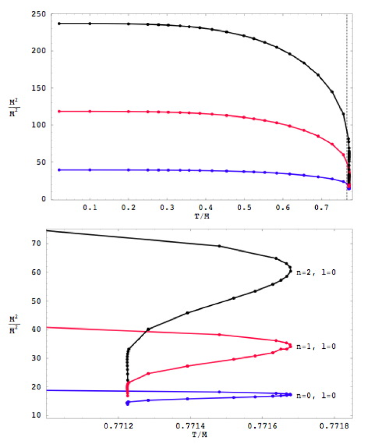
Figure 7: Mass spectrum $M^{2}=\omega^{2}|_{k=0}$ for the $\delta\phi$ fluctuations for Minkowski embeddings in the D3/D7 system.

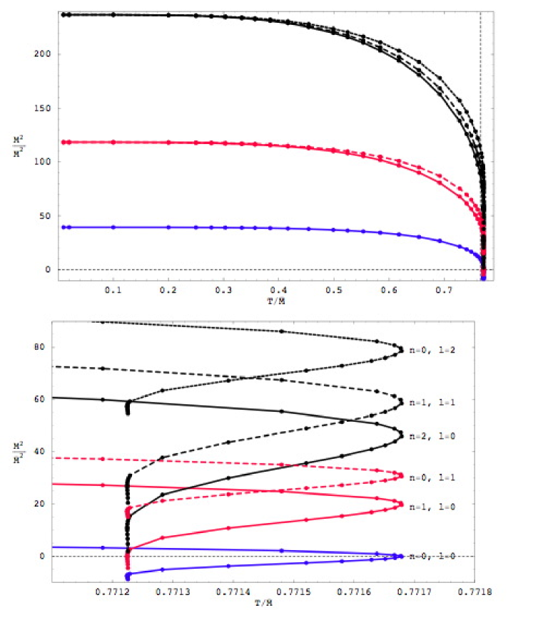
Figure 8: Mass spectrum $M^{2}=\omega^{2}|_{k=0}$ for the $\delta R$ fluctuations for Minkowski embeddings in the D3/D7 system. Note that some of the modes are tachyonic.

At finite temperature, the system is no longer Lorentz invariant and so one must consider the precise definition for the meson masses. We define the ‘rest mass’ of the mesons as the energy $\omega$ with vanishing three-momentum ${\bf k}$ in the rest-frame of the plasma. Thus, solving the equations of motion (75) and (4.3.1) with $\tilde{\bf{k}}=0$ yields the dimensionless constants $\tilde{\omega}^{2}$, which then give the rest masses through (76).

Plots of the mass spectrum for these modes are given in figs. 7 and 8. Note that in the zero-temperature limit, the $\delta R$ and $\delta\phi$ spectra coincide with those previously calculated for the supersymmetric D3 background [9, 10, 11]. In particular, using (48), the lightest meson in both spectra has a mass squared matching $M_{\textrm{\tiny gap}}^{2}=4\pi^{2}\bar{M}^{2}\simeq 39.5\,\bar{M}^{2}$. The degeneracy between the two different modes arises because supersymmetry is restored at $T=0$ and both types of fluctuations are part of the same supermultiplet [9, 10, 11]. At finite $T$, this degeneracy between $\delta R$ and $\delta\phi$ modes is broken. For example, at the phase transition, the mass of the lightest meson is roughly 25% and 50% of its zero-temperature value in the $\delta R$ and $\delta\phi$ spectra, respectively. The supersymmetric spectrum also showed an unexpected degeneracy in that it only depended on the combination $n+\ell_{3}$, where $n$ and $\ell_{3}$ are the radial and angular quantum numbers characterising the individual excitations [9]. Fig. 8 illustrates that this degeneracy is broken at finite temperature, where the masses are shown for all the modes with $n+\ell_{3}=1$ and 2. However, this breaking is not large except near the phase transition.

Both figures show that in general the meson masses decrease as the temperature increases. As noted above, the thermal shift of the meson rest mass may be of the order of 25 to 50 percent at the phase transition. This reduction must reflect in part the decrease in the constituent quark mass, discussed in appendix D. However, the lowering of the meson masses is actually small relative to that seen for the constituent quark mass. As seen in figure 16, at the phase transition, the latter has fallen to only 2% of its $T=0$ value. However, the thermal shift of the mesons becomes even more dramatic near the critical solution. In particular, embeddings with $R_{0}\in(1,1.07)$ possess tachyonic $\delta R$ fluctuations. Note that $R_{0}=1$ corresponds to the critical solutions and the phase transition occurs at $R_{0}\simeq 1.15$, i.e., this is the minimum value of $R_{0}$ for which the thermodynamically preferred embedding is of Minkowski type. As discussed above, the embeddings are not unique in the vicinity of the critical solution and so physical quantities spiral in on their critical values. As observed at the end of section 4.2, the spiralling of the energy density leads to a negative specific heat and indicates an instability. It is satisfying to note in the second plot of fig. 8 that the lowest-lying $\delta R$-mode becomes tachyonic at precisely the point where the first turn-around in the spiral occurs (with $T$). Hence a dynamical instability is appearing in the Minkowski embeddings, in precise agreement with the thermodynamic considerations. In fact the second lowest-lying $\delta R$-mode becomes tachyonic at the second turn-around and it seems to suggest that at the $i$’th turn of the spiral, the $\delta R$-mode with $n=i-1,\ell_{3}=0$ becomes tachyonic. We have found no other evidence of instabilities in other modes. In particular, we have made a detailed examination of the spin-one mesons corresponding to excitations of the worldvolume gauge field. In this case, the observed behaviour is very similar to that of the pseudoscalar $\delta\phi$ modes. It is not surprising that a dynamical instability manifests itself in these $\delta R$-modes, since in the region near the critical solution, the nonuniqueness that brings about the phase transition arises precisely because the branes have slightly different radial profiles $R(r)$.

While a dynamical instability set in for the Minkowski embeddings, in agreement with the thermodynamic analysis, it is interesting that this point is away from the phase transition. In particular, the Minkowski embeddings with $R_{0}\in[1.07,1.15]$, namely those between the point at which the phase transition takes place and the first turn-around, do not exhibit any tachyonic modes. Thus these embeddings are presumably meta-stable and might be reached through super-cooling.

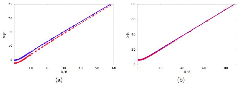
Figure 9: Dispersion relation $\omega(k)$ for Minkowski D7-brane embeddings with (a) $R_{0}=1.20$ ($m=1.32$) and (b) $R_{0}=2.00$ ($m=2.00$) in a D3-brane background. The solid blue line corresponds to $\delta\phi$ fluctuations, whereas the red dashed line corresponds to $\delta R$ fluctuations.

We have also made some preliminary investigations of these low-lying mesons moving through the thermal plasma and numerical results are shown in figure 9. For non-relativistic motion (small three-momenta), we expect that the dispersion relation takes the form

$$\omega(k)\simeq M_{0}+\frac{{\bf k}^{2}}{2M_{kin}}\,,$$ (77)

where $M_{0}=M_{0}(T)$ is the rest mass calculated above and $M_{kin}=M_{\textrm{\tiny kin}}(T)$ is the effective kinetic mass for a moving meson. Although $M_{\textrm{\tiny kin}}(T)$ is not the same as $M_{0}(T)$, for low temperatures the difference between the two quantities is expected to be small. For example, fitting the small-$\tilde{\bf{k}}$ results for $\tilde{\omega}$ for the lowest $\delta R$-mode at $T/\bar{M}=0.5$ (or $R_{0}=2$) yields

$$\frac{\omega}{\bar{M}}=6.084+0.076\frac{{\bf k}^{2}}{\bar{M}^{2}}+\cdots\,.$$ (78)

Hence in this case, we find $M_{0}/\bar{M}\simeq 6.084$ and $M_{\textrm{\tiny kin}}/\bar{M}\simeq 6.579$. Recall that at $T=0$, we would have $M_{0}=M_{\textrm{\tiny kin}}=M_{\textrm{\tiny gap}}=2\pi\bar{M}\simeq 6.283\bar{M}$ and so both masses have shifted by less than 5%. Note that while the rest mass has decreased, the kinetic mass has increased. The latter is perhaps counter-intuitive as it indicates it is actually easier to set the meson in motion through the plasma than in vacuum. From a gravity perspective, it is perhaps less surprising as the Minkowski branes are bending towards the black hole horizon and so these fluctuations experience a greater redshift than in the pure AdS${}_{5}\times S^{5}$ background.

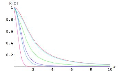
Figure 10: The radial profile for $\delta R$ with $R_{0}=2$ with various spatial momentum. From top to bottom, the profiles correspond to: $k=$ 0, 4.96, 18.81, 31.4, 39.2, 62.7, 94.1.

Examining the regime of large three-momenta, we find that $\omega$ grows linearly with $k$. Naively, one might expect that the constant of proportionality should be one, i.e., the speed of light. However, one finds that

$$\frac{\omega}{\bar{M}}=v_{m}\,\frac{k}{\bar{M}}+\frac{M_{1}}{\bar{M}}+O\left(\frac{\bar{M}}{k}\right)\,.$$ (79)

with $v_{m}<1$, as illustrated in fig. 9. There our numerical results show that for $R_{0}=1.2$ ($m=1.32$), $v_{m}\simeq 0.353$ and $M_{1}/\bar{M}\simeq 4.14$ for $\delta R$ and $v_{m}\simeq 0.350$ and $M_{1}/\bar{M}\simeq 4.71$ for $\delta\phi$, while for $R_{0}=2$ ($m=2$) $v_{m}\simeq 0.884$ and $M_{1}/\bar{M}\simeq 2.61$ for either type of fluctuation. Note that in fig. 9b the dispersion relations $\omega(k)$ for $\delta R$ and $\delta\phi$ are nearly coincident for all $k$ because supersymmetry is being restored at low temperatures. Our results show that the strongly coupled plasma has a significant effect on reducing the maximum velocity of the mesons. This effect is easily understood from the perspective of the dual gravity description. The mesonic states have a radial profile which is peaked near $R_{0}$, the minimum radius of the Minkowski embedding, as illustrated in fig. 10, and so we can roughly think of them as excitations propagating along the bottom of the D7-brane. At large $k$, the speed of these signals will be set by the local speed of light

$$c=\left.\sqrt{-\frac{g_{tt}}{g_{zz}}}\right|_{r=R_{0}}=\frac{f(R_{0})}{\tilde{f}(R_{0})}\,.$$ (80)

The latter gives $c\simeq 0.349$ for $R_{0}=1.2$ and $c\simeq 0.882$ for $R_{0}=2$, both of which closely match our results for $v_{m}$ given above. It is interesting that at finite temperature as $k$ increases, the radial profiles of the mesonic states seem to become more peaked towards $R_{0}$, as illustrated in fig. 10. Recall that at $T=0$, these profiles are invariant under boosts in the gauge theory directions. Finally we note that we did not discover any simple relation between $M_{1}$ in eq. (79) and $M_{0}$ and $M_{kin}$ in eq. (77).

Note that with the approximations made here, our analysis reveals no dragging forces on these low-lying mesons from the thermal bath. We expect that these would only appear through string-loop effects, which in particular would include the Hawking radiation of the background black hole. This would parallel the similar findings for the drag force experienced by large-$J$ mesons composed of heavy quarks [42] and by heavy quarks themselves [43, 44]. These large-$J$ mesons also exhibited a maximum velocity similar to the effect discussed above [42].

5 The D4/D6 system

We now turn to the D4/D6 system, described by the array

$$\begin{array}[]{ccccccccccc}&0&1&2&3&4&5&6&7&8&9\\ D4&\times&\times&\times&\times&\times&&&&&\\ D6&\times&\times&\times&\times&&\times&\times&\times&&\\ \end{array}$$ (81)

In the decoupling limit, the resulting gauge theory is five-dimensional super-Yang-Mills coupled to fundamental hypermultiplets confined to a four-dimensional defect. In order to obtain a four-dimensional gauge theory at low energies, one may compactify $x^{4}$, the D4-brane direction orthogonal to the defect, on a circle. If periodic boundary conditions for the adjoint fermions are imposed, then supersymmetry is preserved and the four-dimensional theory thus obtained is non-confining. In this case the appropriate dual gravitational background at any temperature is (1) with $x^{4}$ periodically identified. Instead, if antiperiodic boundary conditions for the adjoint fermions are imposed, then supersymmetry is broken and the four-dimensional theory exhibits confinement [2] and spontaneous chiral symmetry breaking [5]. The holographic description at zero-temperature consists then of D6-brane probes in a horizon-free background, whose precise form is not needed here. At a temperature $T_{\textrm{\tiny deconf}}$ set by the radius of compactification, the theory undergoes a first order phase transition at which the gluons and the adjoint matter become deconfined. In the dual description the low-temperature background is replaced by (1). If $T_{\textrm{\tiny deconf}}<T_{\textrm{\tiny fun}}$, the D6-branes remain outside the horizon in a Minkowski embedding, and quark-antiquark bound states survive [5]. As $T$ is further increased up to $T_{\textrm{\tiny fun}}$ a first order phase transition for the fundamental matter occurs.

Below we study the thermodynamic and dynamical properties of the D6-branes in the black D4 background appearing above the deconfinement phase transition. Along the way we will have to introduce boundary terms to regulate the D6-brane brane action.

5.1 D6-brane embeddings

As in section 3.3, we begin by transforming to the coordinate system with radial coordinate $\rho$ defined in (24), which is better adapted to study the brane embeddings in the background. For $p=4$, the radial coordinate is then

$$(u_{0}\rho)^{3/2}=u^{3/2}+\sqrt{u^{3}-u_{0}^{3}}\,,$$ (82)

and the black D4-brane metric is

$$ds^{2}=\frac{1}{2}\left(\frac{u_{0}\rho}{L}\right)^{3/2}\left[-\frac{f^{2}}{\tilde{f}}dt^{2}+\tilde{f}dx_{4}^{2}\right]+\left(\frac{L}{u_{0}\rho}\right)^{3/2}\frac{u_{0}^{2}\tilde{f}^{1/3}}{2^{{1/3}}}\left[d\rho^{2}+\rho^{2}d\Omega_{4}^{2}\right]\,,$$ (83)

where we now have $f(\rho)=1-1/\rho^{3}$ and $\tilde{f}(\rho)=1+1/\rho^{3}$. From eq. (6), the temperature is given by

$$T={3\over 4\pi}\left({{u_{0}}\over L^{3}}\right)^{1/2}\,.$$ (84)

We also have the holographic relations for the dual five-dimensional gauge theory

$$L^{3}=\pi g_{\textrm{\tiny s}}N_{\textrm{\tiny c}}\ell_{\textrm{\tiny s}}^{3}\ ,\qquad g_{\textrm{\tiny YM}}^{2}=4\pi^{2}g_{\textrm{\tiny s}}\ell_{\textrm{\tiny s}}\,,$$ (85)

where we remind the reader that the Yang-Mills coupling $g_{\textrm{\tiny YM}}$ is now dimensionful.

The D4/D6 intersection is described by the array (81). In analogy to the D3/D7 case, we introduce spherical coordinates $\{r,\Omega_{2}\}$ in the 567-directions, and polar coordinates $\{R,\phi\}$ on the $89$-plane. Computing boundary terms is also facilitated by introducing an angular coordinate between the $r$ and $R$ directions so that we have, as before,

$$\rho^{2}=r^{2}+R^{2}\,,\,\,\,\,\,r=\rho\sin\theta\,,\,\,\,\,\,R=\rho\cos\theta\,,$$ (86)

and

$$d\rho^{2}+\rho^{2}d\Omega_{4}^{2} = d\rho^{2}+\rho^{2}(d\theta^{2}+\sin^{2}\theta\,d\Omega_{2}^{2}+\cos^{2}\theta\,d\phi^{2})$$ (87)

$$= dr^{2}+r^{2}d\Omega_{2}^{2}+dR^{2}+R^{2}d\phi^{2}\,.$$ (88)

Following our analysis for the D3/D7 system, we choose coordinates on the brane such that asymptotically the metric naturally splits into a product of the form D4-throat$\times S^{2}$. We describe the embedding of the D6-brane in terms of $\chi(\rho)=\cos\theta(\rho)$ – note then that $\chi=R/\rho$. Later, we will have to regulate the Euclidean D6-brane by adding local counter-terms written in terms of this ‘field.’ The induced metric on the D6-brane is then

$$ds^{2}=\frac{1}{2}\left(\frac{u_{0}\rho}{L}\right)^{3/2}\left[-\frac{f^{2}}{\tilde{f}}dt^{2}+\tilde{f}dx_{3}^{2}\right]+\left(\frac{L}{u_{0}\rho}\right)^{3/2}\frac{u_{0}^{2}\tilde{f}^{1/3}}{2^{{1/3}}}\left[\left(1+\frac{\rho^{2}\dot{\chi}^{2}}{1-\chi^{2}}\right)d\rho^{2}+\rho^{2}(1-\chi^{2})d\Omega_{2}^{2}\right]\,,$$ (89)

where, as usual, $\dot{\chi}=d\chi/d\rho$. The D6-brane action takes the form

$$\frac{I_{\textrm{\tiny bulk}}}{{\cal N}}=\int d\rho\,\rho^{2}\,\left(1-\frac{1}{\rho^{6}}\right)\sqrt{(1-\chi^{2})(1-\chi^{2}+\rho^{2}\dot{\chi}^{2})}\,,$$ (90)

where ${\cal N}$ is given by (26) with $n=2$:

$${\cal N}=\frac{\pi}{T}N_{\textrm{\tiny f}}T_{\textrm{\tiny D6}}u_{0}^{3}=\frac{2^{2}}{3^{6}}\,N_{\textrm{\tiny f}}\,N_{\textrm{\tiny c}}\,g_{\textrm{\tiny eff}}(T)^{4}\,T^{3}\,,$$ (91)

where $g_{\textrm{\tiny eff}}(T)^{2}=g_{\textrm{\tiny YM}}^{2}N_{\textrm{\tiny c}}T$. The resulting equation of motion is

$$\partial_{\rho}\left[\rho^{4}\left(1-\frac{1}{\rho^{6}}\right)\frac{\sqrt{1-\chi^{2}}\dot{\chi}}{\sqrt{1-\chi^{2}+\rho^{2}\dot{\chi}^{2}}}\right]+\rho^{2}\left(1-\frac{1}{\rho^{6}}\right)\chi\left[\sqrt{\frac{1-\chi^{2}+\rho^{2}\dot{\chi}^{2}}{1-\chi^{2}}}+\sqrt{\frac{1-\chi^{2}}{1-\chi^{2}+\rho^{2}\dot{\chi}^{2}}}\right]=0\,,$$ (92)

and $\chi$ asymptotically approaches zero as

$$\chi=\frac{m}{\rho}+\frac{c}{\rho^{2}}+\cdots\,,$$ (93)

with $m$ and $c$ related to the quark mass and condensate via eqs. (29) and (30) with $p=4,n=2$:

$$M_{\textrm{\tiny q}} = \frac{u_{0}m}{2^{5/3}\pi\ell_{s}^{2}}={2^{1/3}\over 3^{2}}\,g_{\textrm{\tiny eff}}(T)^{2}\,T\,m\,,$$ (94)

$$\langle{\cal O}_{m}\rangle = -2^{5/3}\pi^{2}\ell_{s}^{2}N_{\textrm{\tiny f}}T_{\textrm{\tiny D6}}u_{0}^{2}c=-\frac{2^{5/3}}{3^{4}}\,N_{\textrm{\tiny f}}\,N_{\textrm{\tiny c}}\,g_{\textrm{\tiny eff}}(T)^{2}T^{3}c\,.$$ (95)

In this case, we may write $m=\bar{M}^{2}/T^{2}$ with

$$\bar{M}^{2}=\frac{9}{2^{1/3}}\left(\frac{M_{\textrm{\tiny q}}}{g_{\textrm{\tiny eff}}(M_{\textrm{\tiny q}})}\right)^{2}\simeq 7.143\left(\frac{M_{\textrm{\tiny q}}}{g_{\textrm{\tiny eff}}(M_{\textrm{\tiny q}})}\right)^{2}\,.$$ (96)

The scale $\bar{M}$ is again related to the mass gap in the meson spectrum of the D4/D6 system at zero temperature. For either background, the latter must be determined numerically. In the case of the supersymmetric background, one finds [10, 11]:

$$m_{\textrm{\tiny gap}}^{2}=8\pi^{2}\,(1.67)\,\left(\frac{M_{\textrm{\tiny q}}}{g_{\textrm{\tiny eff}}(M_{\textrm{\tiny q}})}\right)^{2}\simeq 131.9\left(\frac{M_{\textrm{\tiny q}}}{g_{\textrm{\tiny eff}}(M_{\textrm{\tiny q}})}\right)^{2}\ \longrightarrow\ \frac{\bar{M}}{m_{\textrm{\tiny gap}}}\simeq 0.233\,.$$ (97)

One finds essentially the same result for the confining D4 background [5]. The similarity of these results is probably a reflection of the underlying supersymmetric structure of the five-dimensional gauge theory. In the confining theory, the lowest-lying meson is a pseudo-Goldstone boson, whose mass is determined by the Gell-Mann–Oakes–Renner relation, and the latter linear form extrapolates directly to the supersymmetric result at large $M_{\textrm{\tiny q}}$ [5].

The equation of motion (92) can of course be recast in terms of the $R,r$ coordinates as

$$\partial_{r}\left[r^{2}\left(1-\frac{1}{\rho^{6}}\right)\frac{\partial_{r}R}{\sqrt{1+\left(\partial_{r}R\right)^{2}}}\right]=6\,\frac{r^{2}}{\rho^{8}}\,R\sqrt{1+\left(\partial_{r}R\right)^{2}}\,,$$ (98)

which is again suitable to study the Minkowski embeddings.

For arbitrary $m$ we solved for the D6-brane embeddings numerically. Black hole embeddings are most simply described in the $\chi,\rho$ coordinates and we used boundary conditions at the horizon: $\chi(\rho=1)=\chi_{0}$ and $\dot{\chi}|_{\rho=1}=0$ for various $0\leq\chi_{0}<1$. For Minkowski embeddings, we used the $R,r$ coordinates and the boundary conditions at the axis were: $R(r=0)=R_{0}$ and $\partial_{r}R|_{r=0}=0$ for $R_{0}>1$. We computed $m$ and $c$ by fitting the numerical solutions to the asymptotic forms of $\chi$ and $R$ given above. In particular, we produced plots of $c$ versus $T/\bar{M}$, as shown in figure 11. Again by increasing the resolution, we are able to follow the two families of embeddings spiralling in on the critical solution. However, thermodynamic considerations indicate that a phase transition occurs at the point indicated in the second plot.

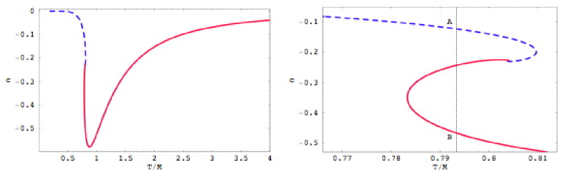
Figure 11: Quark condensate $c$ versus temperature $T/\bar{M}$ for a D6-brane in a D4-brane background. The dotted vertical line indicates the precise temperature of the phase transition.

5.2 D6-brane thermodynamics

As with the D3/D7 system, we wish to compute the contribution of the fundamental matter to the free energy, entropy and energy densities. That is, we will calculate the contributions of the D6-brane to the Euclidean path integral. This requires that we regularise and renormalise the D6-brane action. We will do this by constructing the appropriate counterterms.

Using the asymptotic behaviour (93) in (90) we find that the D6 action contains a UV divergence, since

$$\frac{I_{\textrm{\tiny bulk}}}{{\cal N}}\simeq\int^{\rho_{\textrm{\tiny max}}}d\rho\,\rho^{2}\,\simeq\frac{{\rho_{\textrm{\tiny max}}}}{3}$$ (99)

diverges for ${\rho_{\textrm{\tiny max}}}\to\infty$. We expect the counter-terms that must be supplemented to have the form $\int dt_{\textrm{\tiny E}}d^{3}x\sqrt{\det\gamma}\left(a+b\chi^{2}+c\chi^{4}\right)$. In the present case, we might expect to pick additional factors of $e^{\chi}$ and $e^{\Phi}$. In any event, we would choose the constants to eliminate the divergence. Further for a supersymmetric embedding, we should be able to construct the counter-term action so that the total brane action vanishes.

We take as our ansatz for the counter-terms:

$$I_{\textrm{\tiny bound}}=4\pi L^{3}T_{\textrm{\tiny D6}}\int dt_{\textrm{\tiny E}}d^{3}x\sqrt{\det\gamma}\,e^{2\sigma+B\Phi}F(\chi)\Big{|}_{\rho=\rho_{\textrm{\tiny max}}}\,,$$ (100)

where $B$ and $F(\chi)$ are a dimensionless constant and functional of $\chi$, both to be determined. We have also defined $e^{2\sigma}\equiv g_{\theta\theta}$; this factor naturally appears in the measure as it is proportional to the asymptotic volume of the internal $S^{2}$. Now the boundary metric $\gamma_{ij}$ at $\rho=\rho_{\textrm{\tiny max}}$ in the effective five-dimensional (brane) geometry is given by

$$ds^{2}(\gamma)=\frac{1}{2}\left({u_{0}\rho_{\textrm{\tiny max}}\over L}\right)^{3/2}\left({f^{2}(\rho_{\textrm{\tiny max}})\over\tilde{f}(\rho_{\textrm{\tiny max}})}\,dt_{\textrm{\tiny E}}^{2}+\tilde{f}(\rho_{\textrm{\tiny max}})dx_{3}^{2}\right)$$ (101)

and so $\sqrt{\det\gamma}={1\over 4}\left({u_{0}\rho_{\textrm{\tiny max}}\over L}\right)^{3}f(\rho_{\textrm{\tiny max}})\tilde{f}(\rho_{\textrm{\tiny max}})$. In this coordinate system we have

$$e^{2\Phi}=\frac{1}{2}\left(\frac{u_{0}\rho}{L}\right)^{3/2}\tilde{f}=e^{6\sigma}\,.$$ (102)

Now evaluating the counterterm ansatz (100) with the supersymmetric background ($u_{0}=0$) with the profile $\chi=mu_{0}/\tilde{\rho}$, one finds that the leading divergences cancel if $B=-2/3$ and $F(0)=-1/3$. One also finds that a complete cancellation occurs if we choose

$$F(\chi)=-{1\over 3}(1-\chi^{2})^{3/2}\ .$$ (103)

Thus, the complete counter-term action can be chosen as either of the following:

$$I_{\textrm{\tiny bound}} = -{4\pi\over 3}L^{3}T_{\textrm{\tiny D6}}\int dt_{\textrm{\tiny E}}d^{3}x\sqrt{\det\gamma}\,e^{2\sigma-2\Phi/3}(1-\chi^{2})^{3/2}\Big{|}_{\rho=\rho_{\textrm{\tiny max}}}\,,$$ (104)

$${I^{\prime}}_{\textrm{\tiny bound}} = -{4\pi\over 3}L^{3}T_{\textrm{\tiny D6}}\int dt_{\textrm{\tiny E}}d^{3}x\sqrt{\det\gamma}\,e^{2\sigma-2\Phi/3}\left(1-{3\over 2}\chi^{2}\right)\Big{|}_{\rho=\rho_{\textrm{\tiny max}}}\,.$$ (105)

In the second expression, we have kept only the terms which contribute to the divergence in the small $\chi$ expansion – the next term of ${\cal O}(\chi^{4})$ vanishes as $\rho_{\textrm{\tiny max}}\rightarrow\infty$. Computationally, this seems like the easier action with which to work; note however that the first form has the nice property that, even with finite ${\rho_{\textrm{\tiny max}}}$, it produces a precise cancellation for the supersymmetric configuration, i.e., $I_{\textrm{\tiny D6}}=I_{\textrm{\tiny bulk}}+I_{\textrm{\tiny bound}}=0$.

Proceeding with ${I^{\prime}}_{\textrm{\tiny bound}}$ and using (93), the boundary term evaluates to

$${I^{\prime}}_{\textrm{\tiny bound}}=-\frac{4\pi T_{\textrm{\tiny D6}}}{3T}\left({\rho_{\textrm{\tiny max}}}^{3}-\frac{3}{2}m^{2}{\rho_{\textrm{\tiny max}}}-3mc\right)\,,$$ (106)

where we have divided out the spatial volume $V_{x}$ – see footnote 3. The total action may then be written as:

$$\frac{I\textrm{\tiny D6}}{{\cal N}}=G(m)-\frac{1}{3}\left({\rho_{\textrm{\tiny min}}}^{3}-\frac{3}{2}m^{2}{\rho_{\textrm{\tiny min}}}-3mc\right)\,,$$ (107)

where the integral is defined as

$$G(m)=\int_{\rho_{\textrm{\tiny min}}}^{\infty}d\rho\left[\rho^{2}\left(1-\frac{1}{\rho^{6}}\right)\sqrt{(1-\chi^{2})(1-\chi^{2}+\rho^{2}\dot{\chi}^{2})}-\rho^{2}+\frac{m^{2}}{2}\right]\,.$$ (108)

Of course, the free energy follows from this as $F=TI_{\textrm{\tiny D6}}$ and then one can compute the entropy $S=-\partial F/\partial T$ and the energy $E=F+TS$. For the computation of the entropy, one must split the free energy into bulk and boundary terms and evaluate the action of the derivative on each of the terms, just as was done for the D3/D7 case. We do not present all the details of the calculation here but simply give the final result:

$$\frac{S}{{\cal N}}=-6\,G(m)+2\left({\rho_{\textrm{\tiny min}}}^{3}-\frac{3}{2}m^{2}{\rho_{\textrm{\tiny min}}}-4mc\right)\,,$$ (109)

where the integral $G$ was defined in (108). The contribution of the D6-brane to the energy then follows as

$$\frac{E}{{\cal N}T}=-5\,G(m)+\frac{5}{3}\left({\rho_{\textrm{\tiny min}}}^{3}-\frac{3}{2}m^{2}{\rho_{\textrm{\tiny min}}}-\frac{21}{5}mc\right)\,.$$ (110)

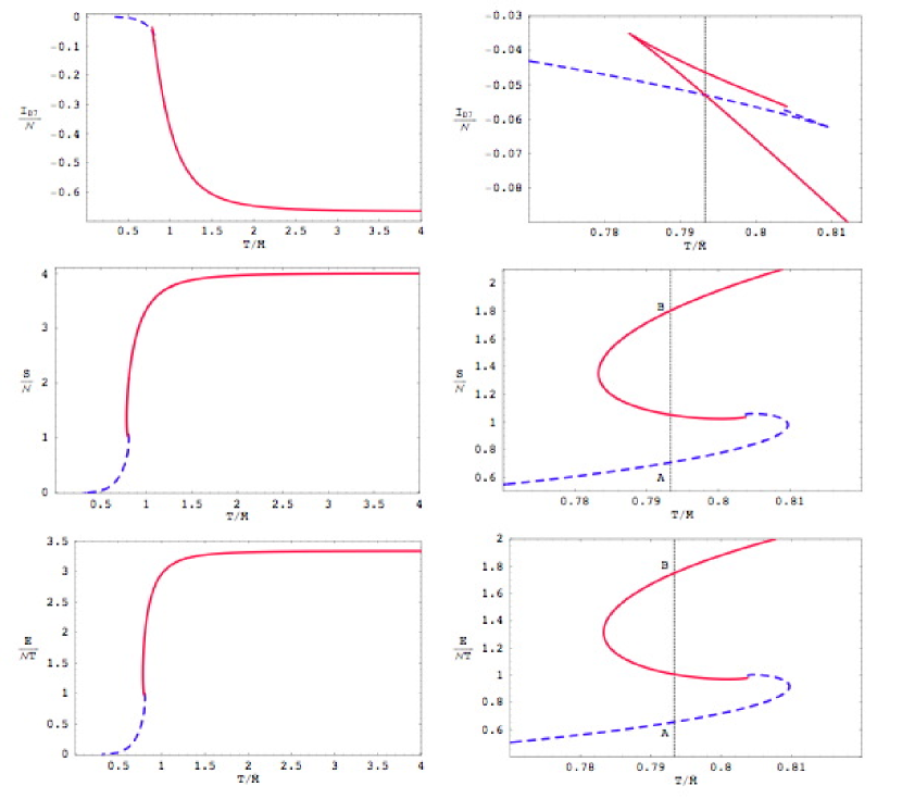
Figure 12: Free-energy, entropy and energy densities for a D6-brane in a D4-brane background. The blue dashed (red continuous) curves correspond to the Minkowski (black hole) embeddings. The dotted vertical line indicates the precise temperature of the phase transition.

Using our numerical results, these thermodynamic quantities are plotted in fig. 12. Again the free energy density shows the classic ‘swallow tail’ form and, to our best numerical accuracy, a first order phase transition takes place at $T_{\textrm{\tiny fun}}/\bar{M}=0.7933$ (or $m=1.589$), where the free energy curves for the Minkowski and black hole phases cross. The fact that the transition is first order is illustrated by the entropy and energy densities, which make a finite jump at this temperature between the points labelled A and B.

5.3 Meson spectrum for Minkowski embeddings

The meson spectrum corresponding to fluctuations of the D6-brane in the black D4-brane geometry is computed in the same way as for D3/D7. We focus here on Minkowski embeddings for which the spectrum is discrete and stable. The excitations of the black hole embeddings will be described by a spectrum of quasinormal modes, as discussed elsewhere [12, 13].

We consider small fluctuations $\delta R,\delta\phi$ about the fiducial embedding, which we now denote by $R_{v}$, so that the D6-brane embedding is specified by $R=R_{v}(r)+\delta R(x^{a})$ and $\phi=0+\delta\phi(x^{a})$, where $R_{v}(r)$ satisfies (98). The pull-back of the bulk metric (83) is then

$$P[G]_{ab}=g_{ab}+\left(\frac{L}{u_{0}\rho}\right)^{3/2}\frac{u_{0}^{2}\tilde{f}^{1/3}}{2^{1/3}}\left\{\dot{R}_{v}\left[(\partial_{a}\delta R)\delta_{b}^{r}+(\partial_{b}\delta R)\delta_{a}^{r}\right]+(\partial_{a}\delta R)\partial_{b}\delta R+R^{2}(\partial_{a}\delta\phi)\partial_{b}\delta\phi\right\}\,,$$ (111)

where the metric $g$ is given by

$$ds^{2}(g)=\frac{1}{2}\left(\frac{u_{0}\rho}{L}\right)^{\frac{3}{2}}\left[-\frac{f^{2}}{\tilde{f}}dt^{2}+\tilde{f}dx_{3}^{2}\right]+\left(\frac{L}{u_{0}\rho}\right)^{\frac{3}{2}}\frac{u_{0}^{2}\tilde{f}^{\frac{1}{3}}}{2^{\frac{1}{3}}}\left[(1+\dot{R}_{v}^{2})dr^{2}+r^{2}d\Omega_{2}^{2}\right]$$ (112)

and, as usual, $\rho^{2}=r^{2}+R^{2}$. The DBI action yields the D6-brane Lagrangian density to quadratic order in the fluctuations $\delta R,\delta\phi$:

$$\mathcal{L} = \mathcal{L}_{0}-T_{\textrm{\tiny D6}}\frac{u_{0}^{3}}{4}r^{2}\sqrt{h}\sqrt{1+\dot{R}_{v}^{2}}\left\{f\tilde{f}\left(\frac{L}{u_{0}\rho_{v}}\right)^{3/2}\frac{u_{0}^{2}\tilde{f}^{1/3}}{2^{4/3}}\sum_{a}g_{v}^{aa}\left[\frac{(\partial_{a}\delta R)^{2}}{1+\dot{R}_{v}^{2}}+R^{2}(\partial_{a}\delta\phi)^{2}\right]\right.$$ (113)

$$+\left.\frac{3R_{v}\dot{R}_{v}\partial_{r}(\delta R)^{2}}{\rho_{v}^{8}(1+\dot{R}_{v}^{2})}+\frac{3(\delta R)^{2}}{\rho_{v}^{8}}-\frac{24R_{v}^{2}(\delta R)^{2}}{\rho_{v}^{10}}\right\}\,,$$

where $h$ is the determinant of the metric on the $S^{2}$ of unit radius, $\rho_{v}^{2}=r^{2}+R_{v}^{2}$, and $\mathcal{L}_{0}$ is the Lagrangian density for the vacuum embedding:

$$\mathcal{L}_{0}=-T_{\textrm{\tiny D6}}\frac{u_{0}^{3}}{4}r^{2}\sqrt{h}\sqrt{1+\dot{R}_{v}^{2}}\left(1-\frac{1}{\rho_{v}^{6}}\right).$$ (114)

Note that terms linear in $\delta R$ were eliminated from the Lagrangian density $\mathcal{L}$ by integration by parts and by using the equation of motion (98) for $R_{v}$. Since we are retaining terms only to quadratic order in the fluctuations, the metric $g_{v}$ in (113) is (112) with $R=R_{v}$ and the functions $f$ and $\tilde{f}$ in (113) and subsequent expressions are evaluated at $\rho_{v}$.

The linearised equations of motion for the fluctuations are then

$$\partial_{a}\left[f\tilde{f}\left(\frac{L}{u_{0}\rho_{v}}\right)^{3/2}\frac{u_{0}^{2}\tilde{f}^{1/3}}{2^{1/3}}r^{2}\sqrt{h}R_{v}^{2}\sqrt{1+\dot{R}_{v}^{2}}\,g_{v}^{ab}\,\partial_{b}\delta\phi\right]=0$$ (115)

for $\delta\phi$, and

$$\partial_{a}\left[f\tilde{f}\left(\frac{L}{u_{0}\rho_{v}}\right)^{3/2}\frac{u_{0}^{2}\tilde{f}^{1/3}}{2^{1/3}}\frac{r^{2}\sqrt{h}}{\sqrt{1+\dot{R}_{v}^{2}}}\,g_{v}^{ab}\,\partial_{b}\delta R\right]$$

$$\qquad\qquad=6\frac{r^{2}}{\rho_{v}^{8}}\sqrt{h}\sqrt{1+\dot{R}_{v}^{2}}\left(1-\frac{8R_{v}^{2}}{\rho_{v}^{2}}\right)\delta R-6\sqrt{h}\partial_{r}\left(\frac{r^{2}}{\sqrt{1+\dot{R}_{v}^{2}}}\frac{R_{v}\dot{R}_{v}}{\rho_{v}^{8}}\right)\delta R$$

for $\delta R$. Proceeding via separation of variables, we take

$$\delta\phi=\mathcal{P}(r)\mathcal{Y}^{\ell_{2}}(S^{2})\,e^{-i\omega t}e^{i{\bf k}\cdot{\bf x}},\quad\delta R=\mathcal{R}(r)\mathcal{Y}^{\ell_{2}}(S^{2})\,e^{-i\omega t}e^{i{\bf k}\cdot{\bf x}}\,$$ (116)

where $\mathcal{Y}^{\ell_{2}}(S^{2})$ are spherical harmonics on the $S^{2}$ of unit radius satisfying $\nabla^{2}_{S^{2}}\mathcal{Y}^{\ell_{2}}=-\ell_{2}(\ell_{2}+1)\mathcal{Y}^{\ell_{2}}$. We obtain the radial differential equation

$$\partial_{r}\left[\frac{r^{2}f\tilde{f}R_{v}^{2}}{\sqrt{1+\dot{R}_{v}^{2}}}\partial_{r}\mathcal{P}\right]+fR_{v}^{2}\sqrt{1+\dot{R}_{v}^{2}}\left[2^{2/3}\frac{r^{2}}{\rho_{v}^{3}}\tilde{f}^{1/3}\left(\frac{\tilde{f}^{2}}{f^{2}}\tilde{\omega}^{2}-\tilde{\bf{k}}^{2}\right)-\ell_{2}(\ell_{2}+1)\tilde{f}\right]\mathcal{P}=0$$ (117)

for $\delta\phi$ and

$$\partial_{r}\left[\frac{r^{2}f\tilde{f}}{(1+\dot{R}_{v}^{2})^{\frac{3}{2}}}\partial_{r}\mathcal{R}\right]+\frac{f}{\sqrt{1+\dot{R}_{v}^{2}}}\left[2^{2/3}\frac{r^{2}}{\rho_{v}^{3}}\tilde{f}^{1/3}\left(\frac{\tilde{f}^{2}}{f^{2}}\tilde{\omega}^{2}-\tilde{\bf{k}}^{2}\right)-\ell_{2}(\ell_{2}+1)\tilde{f}\right]\mathcal{R}$$

$$\qquad\qquad=6\left[\frac{r^{2}}{\rho_{v}^{8}}\sqrt{1+\dot{R}_{v}^{2}}\left(1-\frac{8R_{v}^{2}}{\rho_{v}^{2}}\right)-\partial_{r}\left(\frac{r^{2}R_{v}\dot{R}_{v}}{\rho_{v}^{8}\sqrt{1+\dot{R}_{v}^{2}}}\right)\right]\mathcal{R}$$

for $\delta R$. The dimensionless constant $\tilde{\omega}$ is related to $\omega$ via

$$\omega^{2}=\tilde{\omega}^{2}\frac{u_{0}}{L^{3}}=\tilde{\omega}^{2}\left(\frac{4\pi}{3}\right)^{2}{T^{2}}=\tilde{\omega}^{2}\left(\frac{4\pi}{3}\right)^{2}\frac{\bar{M}^{2}}{m}\,,$$ (118)

and analogously for $\tilde{\bf{k}}$.

We solved (5.3) and (117) numerically and determined the eigenvalues $\tilde{\omega}$ using a shooting method, as was done in the D3/D7 case. The masses are given by $M^{2}=\omega^{2}$ in the frame in which the three momentum vanishes: ${\bf k}=0$. The spectra $M^{2}/\bar{M}^{2}$ versus $T/\bar{M}$ for the angular fluctuations $\delta\phi$ and the radial fluctuations $\delta R$ are presented in figs. 13 and 14, respectively (both for $\ell=0$), and are qualitatively the same as those for the D3/D7 system: the $\delta R$ and $\delta\phi$ modes become degenerate in the zero-temperature limit, reflecting supersymmetry restoration; in general the meson masses decrease as the temperature increases, especially near the critical solution; and the results for $\delta R$ fluctuations suggest that a new mode becomes tachyonic at each turn-around of the curves.

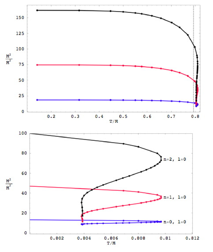
Figure 13: Mass spectrum $M^{2}=\omega^{2}|_{k=0}$ for the $\delta\phi$ fluctuations for Minkowski embeddings in the D4/D6 system. The dashed vertical line marks the phase transition.

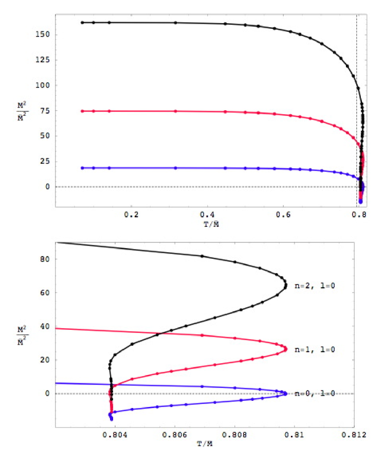
Figure 14: Mass spectrum $M^{2}=\omega^{2}|_{k=0}$ for the $\delta R$ fluctuations for Minkowski embeddings in the D4/D6 system. The dashed vertical line marks the phase transition while the dotted horizontal line marks $M^{2}=0$. Note that some modes become tachyonic.

6 Discussion

We have shown that, in a large class of strongly coupled gauge theories with fundamental fields, this fundamental matter undergoes a first order phase transition at some high temperature $T_{\textrm{\tiny fun}}\sim\bar{M}$, where $\bar{M}$ is a scale characteristic of the meson physics. As well as giving the mass gap in the meson spectrum [9], $1/\bar{M}$ is roughly the characteristic size of these bound states [45, 11]. In our models, the gluons and other adjoint fields were already in a deconfined phase at $T_{\textrm{\tiny fun}}$, so this new transition is not a confinement/deconfinement transition. Neither is it a chiral symmetry-restoration phase transition, since the chiral condensate $\langle\bar{\psi}\psi\rangle\propto c$ that breaks the axial $U(1)_{\textrm{\tiny A}}$ symmetry does not vanish above $T_{\textrm{\tiny fun}}$. The most striking feature of the new phase transition is the change in the meson spectrum and so we refer to it as a ‘dissociation’ or ‘melting’ transition.

In the low-temperature phase, below the transition, the mesons are deeply bound and the spectrum is discrete and gapped. To leading order in the large-$N_{\textrm{\tiny c}}$ expansion these states are absolutely stable, but at higher orders they may decay into other mesons of lower mass or glueballs. The leading channel is one-to-two meson decay and after examining the interactions in the effective action [9], we find that parametrically the width of a typical state is given by $M_{\textrm{\tiny q}}/(N_{\textrm{\tiny c}}\,\lambda^{3/2})\simeq M_{\textrm{\tiny gap}}/(N_{\textrm{\tiny c}}\,\sqrt{\lambda})$. Recall that this is not a confining phase and so we can also introduce free quarks into the system. Of course, such a quark is represented by a fundamental string stretching between the D7-branes and the horizon. At a figurative level, in this phase, we might describe quarks in the adjoint plasma as a ‘suspension’. That is, when quarks are added to this phase, they retain their individual identities.

Above the phase transition (i.e., at $T>T_{\textrm{\tiny fun}}$), the meson spectrum is continuous and gapless. The excitations of the fundamental fields would be characterised by a discrete spectrum of quasinormal modes on the black hole embeddings [12, 13]. Investigations of the spectral functions [13] show that some interesting structure remains near the phase transition. Some of these excitations may warrant an interpretation in terms of quasiparticle excitations but in any event, there are only a few such states in contrast with the (nominally) infinite spectrum of mesons found in the low temperature phase. An appropriate figurative characterisation of the quarks in this high temperature phase would be as a ‘solution’. If one attempts to inject a localised quark charge into the system, it quickly spreads out across the entire plasma and its presence is reduced to diffuse disturbances of the supergravity and worldvolume fields, which are soon damped out [12, 13].

The physics above is potentially interesting in connection with QCD, since lattice simulations indicate that heavy-quark mesons indeed remain bound in a range of temperatures above $T_{\textrm{\tiny deconf}}$. For example, for the lightest charmonium states, the melting temperature may be conservatively estimated to be around $1.65T_{\textrm{\tiny deconf}}\simeq 249$ to $317$ MeV [14, 15], depending on the precise value of $T_{\textrm{\tiny deconf}}$ [17]. Some other studies suggest that the $J/\psi(1S)$ state may persist to $\sim 2.1T_{\textrm{\tiny deconf}}\simeq 317$ to $403$ MeV [16]. In the D3/D7 model, we see from fig. 5 that quark-antiquark bound states melt at $T_{\textrm{\tiny fun}}\simeq 0.766\bar{M}$. The scale $\bar{M}$ is related to the mass $M^{\ast}=M_{\textrm{\tiny gap}}$ of the lightest meson in the theory at zero temperature through eq. (48). Therefore we have $T_{\textrm{\tiny fun}}(M^{\ast})\simeq 0.122M^{\ast}$. For the charmonium states above, taking $M^{\ast}\simeq 3000$ MeV gives $T_{\textrm{\tiny fun}}(c\bar{c})\simeq 366$ MeV. Similarly, for the D4/D6 system we have (97) which yields $\bar{M}\simeq 0.233M^{*}$. The transition temperature in this case is then $T_{\textrm{\tiny fun}}\simeq 0.793\bar{M}\simeq 0.186M^{\ast}$, which gives $T_{\textrm{\tiny fun}}(c\bar{c})\simeq 557$ MeV. Hence it is gratifying that these comparisons lead to a qualitative agreement with the lattice results.

Of course, these comparisons must be taken with some caution, since meson bound states in Dp/Dq systems are deeply bound, i.e., $M^{\ast}\ll 2M_{q}$, whereas the binding energy of charmonium states is a small fraction of the charm mass, i.e., $M_{c\bar{c}}\simeq 2M_{c}$. It might then be more appropriate to compare with lattice results for $s\bar{s}$ bound states which are also seen to survive the deconfinement transition. For the $\phi$-meson, whose mass is $M_{\phi}\simeq 1020$ MeV, the formulas above yield $T_{\textrm{\tiny fun}}(s\bar{s})\simeq 124$ MeV (D3/D7) and $T_{\textrm{\tiny fun}}(s\bar{s})\simeq 188$ MeV (D4/D6). Lattice simulations suggest that the melting temperature is around $1.4T_{\textrm{\tiny deconf}}\simeq 211$ to $269$ MeV [47, 15]. While again we have qualitative agreement, one must observe that at least for the D3/D7 calculation, our result lies below even the lowest estimate for $T_{\textrm{\tiny deconf}}\simeq 151$ MeV.

An additional caveat is that here we have identified the melting temperature with $T_{\textrm{\tiny fun}}$, above which the discrete meson states disappear. However, the spectral function of some two-point meson correlators in the holographic theory still exhibit some broad peaks in a regime just above $T_{\textrm{\tiny fun}}$, which suggests that a few bound states persist just above the phase transition [13]. This is quite analogous to the lattice approach where similar spectral functions are used to examine the existence or otherwise of the bound states. Hence using $T_{\textrm{\tiny fun}}$ above should be seen as a (small) underestimate of the melting temperature.

Before leaving this discussion of comparisons with QCD, we reiterate that the present holographic calculations are examining exotic gauge theories and so any agreements above must be regarded with a skeptical eye. However, we would also like to point out one simple physical parallel between all of these systems. The question of charmonium bound states surviving in the quark-gluon plasma was first addressed by comparing the size of the bound states to the screening length in the plasma [48]. While the original calculations have seen many refinements (see, e.g., [49]), the basic physical reasoning remains sound and so we might consider applying the same argument to the holographic gauge theories. Considering first the ${\cal N}=2$ SYM theory arising from the D3/D7 system, the size of the mesons can be inferred from the structure functions in which the relevant length scale which emerges is $\sqrt{\lambda}/M_{\textrm{\tiny q}}$ [45]. Holographic studies of Wilson lines in a thermal bath [50] show that the relevant screening length of the SYM plasma is order $1/T$. In fact, the same result emerges from a field theoretic scheme of hard-thermal-loop resummation applied to SYM theories [51]. In any event, combining these results, the argument that the mesons should dissociate when the screening length is shorter than the size of these bound states yields $T\sim M_{\textrm{\tiny q}}/\sqrt{\lambda}$. Of course, the latter matches the results of our detailed calculations in section 4. The same reasoning can be applied to the D4/D6 system where the meson size is $O(g_{\textrm{\tiny eff}}(M_{\textrm{\tiny q}})/M_{\textrm{\tiny q}})$ [11] and the screening length is again $O(1/T)$ [52]. Hence this line of reasoning again leads to a dissociation temperature in agreement with the results of section 5. Therefore we see that the same physical reasoning which was used so effectively for the $J/\psi$ in the QCD plasma can also be used to understand the dissociation of the mesons in the present holographic gauge theories.

One point worth emphasising is that there are two distinct processes that are occurring at $T\sim\bar{M}$. If we consider, e.g., the entropy density in fig. 5, we see that the phase transition occurs in the midst of a cross-over signalled by a rise in $S/T^{3}$. We may write the contribution of the fundamental matter to entropy density as

$$S_{\textrm{\tiny fun}}=\frac{1}{8}\lambda\,N_{\textrm{\tiny f}}\,N_{\textrm{\tiny c}}\,T^{3}\ H\!\left(\frac{T^{2}}{M_{\textrm{\tiny q}}^{2}/\lambda}\right)$$ (119)

where $H(x)$ is the function plotted in fig. 5. $H$ rises from 0 at $x=0$ to 2 as $x\rightarrow\infty$ but the most dramatic part of this rise occurs in the vicinity of $x=1$. Hence it seems that new degrees of freedom, i.e., the fundamental quarks, are becoming ‘thermally activated’ at $T\sim\bar{M}$. We might note that the phase transition produces a discontinuous jump in which $H$ only increases by about 0.07, i.e., the jump at the phase transition only accounts for about 3.5% of the total entropy increase. Thus the phase transition seems to play an small role in this cross-over and produces relatively small changes in the thermal properties of the fundamental matter, such as the energy and entropy densities.

As $\bar{M}$ sets the scale of the mass gap in the meson spectrum, it is tempting to associate the cross-over above with the thermal excitation of mesonic degrees of freedom. However, the pre-factor $\lambda\,N_{\textrm{\tiny f}}\,N_{\textrm{\tiny c}}$ in (119) indicates that this reasoning is incorrect. If mesons provided the relevant degrees of freedom, we should have $S_{\textrm{\tiny fun}}\propto N_{\textrm{\tiny f}}^{2}$. Instead the factor of $N_{\textrm{\tiny f}}N_{\textrm{\tiny c}}$ is naturally interpreted as counting the number of degrees of freedom associated with free quarks, with the factor $\lambda$ demonstrating that the contribution of the quarks is enhanced at strong coupling. A complementary interpretation of (119) comes from reorganizing the pre-factor as:

$$\lambda\,N_{\textrm{\tiny f}}\,N_{\textrm{\tiny c}}=(g_{\textrm{\tiny YM}}^{2}\,N_{\textrm{\tiny f}})\,N_{\textrm{\tiny c}}^{2}\,.$$ (120)

The latter expression makes clear that the result corresponds to the first order correction of the adjoint entropy due to loops of fundamental matter. As discussed in [34], we are working in a ‘not quite’ quenched approximation, in that thermal contributions of the D7-branes represent the leading order contribution in an expansion in $N_{\textrm{\tiny f}}/N_{\textrm{\tiny c}}$, and so fundamental loops are suppressed but not completely. In [34], it was shown that the expansion for the classical gravitational back-reaction of D7-brane is controlled by $\lambda N_{\textrm{\tiny f}}/N_{\textrm{\tiny c}}=g_{\textrm{\tiny YM}}^{2}\,N_{\textrm{\tiny f}}$. Hence this expansion corresponds to precisely the expansion in loops of fundamental matter. However, naively the fundamental loops would be suppressed by factors of $T^{2}/M_{\textrm{\tiny q}}^{2}$ coming from the quark propagators. So from this point of view, the strong coupling enhancement corresponds to the fact that such factors only appear as $\lambda\,T^{2}/M_{\textrm{\tiny q}}^{2}$ in eq. (119).

Hence the strongly coupled theory brings together these two otherwise distinct processes. That is, at strong coupling, the dissociation of the bound states and the thermal activation of the fundamental matter happen at essentially the same temperature. While our discussion above focused on the D3/D7 system, the D4/D6 results exhibit the same behaviour. Hence this seems to be a universal feature of the holographic gauge theories described by Dp/Dq systems.

The preceding behaviour might be contrasted with that which is expected to occur at weak coupling. In this regime, one expects that the melting of the mesons would also be a cross-over rather than a (first-order) phase transition. Moreover, the temperature at which the mesons dissociate would be $T_{\textrm{\tiny fun}}\sim E_{\textrm{\tiny bind}}\sim g_{\textrm{\tiny eff}}^{4}M_{\textrm{\tiny q}}$. On the other hand, the quarks would not be thermally activated until we reach $T_{\textrm{\tiny activ}}\sim 2M_{\textrm{\tiny q}}$, at which point free quark-antiquark pairs would be readily produced. Of course, the thermal activation would again correspond to a cross-over rather than a phase transition. The key point, which we wish to emphasise, is that these two temperatures are widely separated at weak coupling.

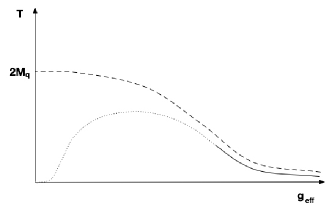
Figure 15: A qualitative representation of the simplest possibility interpolating between the weak and the strong coupling regimes. The solid and the dotted lines correspond to $T=T_{\textrm{\tiny fun}}$. At strong coupling this corresponds to a first-order phase transition (solid line), whereas at weak coupling it corresponds to a cross-over (dotted line). The dashed line corresponds to $T=T_{\textrm{\tiny activ}}$. At strong-coupling this takes place immediately after the phase transition, whereas at weak coupling it is widely separated from $T_{\textrm{\tiny fun}}$.

Fig. 15 is an ‘artistic’ representation of the simplest behaviour which would interpolate between strong and weak coupling. One might expect that the melting point and the thermal activation are very close for $g_{\textrm{\tiny eff}}\gg 1$. The line of first order phase transitions must end somewhere and so one might expect that it terminates at a critical point around $g_{\textrm{\tiny eff}}\sim 1$. Below this point, both processes would only represent cross-overs and their respective temperatures would diverge from one another, approaching the weak coupling behaviour described above.

There are two aspects to enhancement of the thermal densities discussed above. First, at strong coupling the fundamental matter has a stronger effect on the nonabelian plasma than might have been otherwise guessed and second the effect is a positive one. That is, e.g., the energy and entropy densities are raised. Because we are working with $N_{\textrm{\tiny f}}/N_{\textrm{\tiny c}}\ll 1$, the enhancement we observe is a small correction to the overall properties of the plasma. In fact, it can be added to a list of such correction terms, with others arising as finite-$\lambda$ [53] and finite-$N_{\textrm{\tiny c}}$ effects. Both of these types of corrections are expected to raise the entropy and energy densities of the plasma, as well.

As our calculations were also performed in the limit $N_{\textrm{\tiny c}},\lambda\rightarrow\infty$ (with $N_{\textrm{\tiny f}}$ fixed), it is natural to ask how the detailed results of our paper depend on this approximation. First of all, the fact that the phase transition is first order implies that it should be stable under small perturbations and so its order and other qualitative details should hold within a finite radius of the $1/N_{\textrm{\tiny c}},1/\lambda$ expansions. Of course, finite-$N_{\textrm{\tiny c}}$ and finite-$\lambda$ corrections may eventually modify the behaviour uncovered here. For example, at large but finite $N_{\textrm{\tiny c}}$ the black hole will Hawking-radiate and each bit of the brane probe will experience a thermal bath at a temperature determined by the local acceleration. This effect becomes more and more important as the lower part of a Minkowski brane approaches the horizon, and may potentially blur the self-similar, scaling behaviour found here. However, at the phase transition, the minimum separation of brane embeddings and the horizon is not parametrically small. For example, $R_{0}=1.1538$ at the transition for D3/D7 system. Hence while the Hawking radiation can be expected to interfere with the self-similar behaviour near the critical embedding, it should not disturb the phase transition for large but finite $N_{\textrm{\tiny c}}$.

Finite ’t Hooft coupling corrections correspond to higher-derivative corrections both to the supergravity action and the D-brane action. These may also blur the details of the structure discussed above. For example, higher-derivative corrections to the D-brane equation of motion are likely to spoil the scaling symmetry of eq. (19), and hence the self-similar behaviour. These corrections will again become important near the critical solution, for both Minkowski and black hole embeddings, since the (intrinsic) curvature of the brane becomes large there. However, the phase transition should remain robust for large but finite $\lambda$ because at this point, the separation of brane embeddings from the critical solution is not parametrically small. We illustrated this for the Minkowski embedding at the phase transition of D3/D7 above but here we can add the same is true for the black hole embedding at this point, which has $\chi_{0}=0.9427$.

Another significant set of corrections come from the gravitational backreaction of the D7-branes (or more generally the probe Dq-branes) on the background spacetime or from fundamental loops in the gauge theory. As indicated above, these are dual descriptions of the same expansion. Our results only represent the first contribution in an infinite series of terms, whose magnitudes are controlled by the ratio $N_{\textrm{\tiny f}}/N_{\textrm{\tiny c}}$. Given that low energy QCD has $N_{\textrm{\tiny f}}/N_{\textrm{\tiny c}}=1$, it is of particular interest to study holographic theories in Veneziano’s limit of $g_{\textrm{\tiny YM}}\rightarrow 0$, $N_{\textrm{\tiny c}}\rightarrow\infty$ with both $\lambda$ and $N_{\textrm{\tiny f}}/N_{\textrm{\tiny c}}$ finite [54]. A variety of attempts have been made to construct gravitational backgrounds describing gauge theories in this limit [55].

The D2/D6 system provides one interesting background where this limit was studied at finite temperature [56]. In particular, it was found that the energy density scales as $F\sim N_{\textrm{\tiny f}}^{1/2}N_{\textrm{\tiny c}}^{3/2}T^{3}$, which obviously differs from (33) with $p=2,d=2$. This discrepancy is not at all a contradiction and has the same origin as the discrepancy found for the meson spectrum [10, 11]. This is the fact that the calculation in [56] applies in the far infrared of the gauge theory, whereas that presented here applies at high temperatures, i.e., at $T\gg g_{\textrm{\tiny YM}}^{2}$.

We close with a few more observations. Ref. [58] argued for the existence of plasma balls in a broad class of confining large-$N_{\textrm{\tiny c}}$ theories, which undergo first order deconfinement phase transitions. That is, in these theories, one could form metastable, localised lumps of deconfined gluon plasma. Their dual description should consist of black holes localised along some gauge theory directions. One may imagine an analogous construction for the fundamental matter, based on the first order phase transition discussed here. That is, near $T_{\textrm{\tiny fun}}$ one should be able to construct inhomogenous brane configurations in which only a localised region on the branes has fallen through the black hole horizon, i.e., the induced brane metric would contain a localised black hole. The dual gauge theory interpretation would be in terms of a localised bubble inside of which the fundamental matter has melted. Such bubbles may be of interest for understanding how the melting transition actually occurs in a dynamical context.

Finally, we comment on the ‘quark condensate’ at high temperatures. If one examines fig. 4 for example, it is tempting to infer that, since $c$ approaches zero as $T\rightarrow\infty$, the quark condensate vanishes in this limit. This vanishing would then be in agreement with the intuition that at high temperatures the thermal fluctuations should destroy any coherent condensate. However, vanishing $c$ is not enough to ensure that $\langle{\cal O}_{m}\rangle$ also vanishes. In fact, if we combine eqs. (47) and (130), we see that at high temperatures the condensate actually grows as

$$\langle{\cal O}_{m}\rangle\sim N_{\textrm{\tiny c}}N_{\textrm{\tiny f}}M_{\textrm{\tiny q}}T^{2}\,.$$ (121)

At this point, it is important to recall the form of the full operator ${\cal O}_{m}$ given in eq. (31). The first two terms are dimension-three operators and so in the high temperature limit we can expect the magnitude of typical fluctuations in these to be $O(T^{3})$. Further these operators do not have a definite sign and so presumably their expectation value vanishes when averaging over all fluctuations in the disordered high-temperature system. This, of course, is the basis of the intuition that $\langle\bar{\psi}\psi\rangle\rightarrow 0$. Now the last term in eq. (31) is only a dimension-two operator and so we expect thermal fluctuations to be of $O(T^{2})$. The key difference in this case is that the operator only takes positive real values and so averaging over all fluctuations we expect $\langle q^{\dagger}q\rangle\propto T^{2}$. Hence our calculations make a precise prediction for this expectation value in the high-temperature phase. Note though that this is a thermal expectation value and not a coherent (zero-momentum) condensate, which we expect that we are observing with $\langle{\cal O}_{m}\rangle\neq 0$ at low temperatures.

Hence it is interesting that the high temperature phase seems to display two distinct regimes of behaviour. At very high temperatures, the physics is dominated by incoherent thermal fluctuations of the fundamental fields, as expected. However, there is also a regime just above the phase transition where the system can support a coherent condensate. This regime would correspond to the region where $|c|/T^{3}$ is still growing in fig. 4. Of course, there is a cross-over between these two regimes and so there is only a rough boundary. It may be natural to define the latter as the point where $c$ is extremized, i.e., $T\simeq 1.2\bar{M}$. Again, this seems to be a universal property of the broad class of holographic theories described by Dp/Dq systems. For example, fig. 11 indicates the same behaviour for D6-branes in a D4 background.

The above seems to be one more facet of the rich phenomenology which these holographic theories display at finite temperature. However, this phenomenology presents several puzzles, such as why $T_{\textrm{\tiny fun}}\sim\bar{M}$ rather than $M_{\textrm{\tiny q}}$ is the scale at which the bound states melt or at which the free quarks are thermally excited. For example, the former seems counterintuitive in view of the fact that, in the regime of strong coupling considered here, this temperature is much lower than the binding energy of the mesons:

$$E_{\textrm{\tiny bind}}\sim 2M_{\textrm{\tiny q}}-\bar{M}\sim 2M_{\textrm{\tiny q}}\,.$$ (122)

However, this intuition relies on the expectation that the result of melting a meson is a free quark-antiquark pair of mass $2M_{\textrm{\tiny q}}$. The gravity description makes it clear that this is not the case at strong coupling. In fact, the constituent quark mass vanishes when the branes fall into the horizon – see appendix D. Rather, in this regime the system is better thought of as a strongly coupled liquid of both adjoint and fundamental fields.

In any event, it is gratifying that the holographic description of these gauge theories with fundamental matter provides once more an extremely simple, geometric interpretation of some complicated, strong-coupling physics, such as the existence or otherwise of stable quark-antiquark bound states above the deconfinement temperature. Other well known examples include the geometric characterisations of confinement [2, 59] and chiral symmetry breaking [4, 5, 8, 60].

Appendix A Embeddings for high and low temperatures for D3/D7

A.1 High temperatures (black hole embeddings)

Consider the limit $T/\bar{M}\gg 1$. This corresponds to black hole embeddings with $m=\bar{M}/T\ll 1$. As usual, we use the $\chi,\rho$ coordinates. Note that the equatorial D7-brane embedding, $\chi=0$, is an exact solution of the equation of motion (44). To study nearby solutions we expand the bulk portion of the D7-brane action (42) to quadratic order in $\chi$

$${I_{\textrm{\tiny bulk}}\over{\cal N}}\simeq\int_{1}^{\infty}d\rho\left(1-{1\over\rho^{8}}\right)\rho^{3}\left(1-{3\over 2}\chi^{2}+{1\over 2}\dot{\chi}^{2}\right)\,,$$ (123)

thus obtaining the linearised equation of motion:

$$\partial_{\rho}\left[\left(1-{1\over\rho^{8}}\right)\rho^{5}\dot{\chi}\right]=-3\left(1-{1\over\rho^{8}}\right)\rho^{3}\chi\,.$$ (124)

To solve this equation, it is useful to make the change of variables $x=\rho^{2}$ so that it becomes:

$$x(x^{4}-1)(4x\chi^{\prime\prime}+2\chi^{\prime})+2x(5x^{4}+3)\chi^{\prime}+3(x^{4}-1)\chi=0$$ (125)

where $\chi^{\prime}=d\chi/dx$. The solution of this equation satisfying the boundary condition $\chi^{\prime}|_{x=1}=0$ is

$$\tilde{\chi}={4\over 45\left[\Gamma\left({1\over 4}\right)\right]^{2}}\left[9\Gamma\left({5\over 4}\right)\Gamma\left({9\over 4}\right)x^{1/2}F\left({1\over 4},{1\over 2};{3\over 4};x^{4}\right)-5\left[\Gamma\left({7\over 4}\right)\right]^{2}x^{3/2}F\left({1\over 2},{3\over 4};{5\over 4};x^{4}\right)\right]\,,$$ (126)

where $F(a,b;c;z)$ is the hypergeometric function satisfying

$$z(1-z)F^{\prime\prime}+[c-(a+b+1)z]F^{\prime}-abF=0.$$ (127)

The overall normalization of the solution is arbitrary since, we are solving a linear equation. In the above, we have chosen the normalization such that

$$\tilde{\chi}\simeq 1/x^{1/2}+\tilde{c}/x^{3/2}\,,\quad x\to\infty$$ (128)

where

$$\tilde{c}={\Gamma\left({-1\over 4}\right)\Gamma\left({3\over 4}\right)^{2}\over\sqrt{2}\pi\Gamma\left({1\over 4}\right)}\simeq-0.456947.$$ (129)

The tilde on the solution $\tilde{\chi}$ and condensate $\tilde{c}$ indicate that these is the solution for unit mass. The general solution for arbitrary small mass (or equivalently, high temperatures) is simply $\chi=m\tilde{\chi}$ and the condensate is given by

$$c=m\tilde{c}\,.$$ (130)

A.2 Low temperatures (Minkowski embeddings)

Low-temperature solutions correspond to Minkowski embeddings in which the D7 probe is very far from the horizon: $R_{0}\gg 1$ or, equivalently, $m=\bar{M}/T\gg 1$. In this case, we expect the brane profile to be nearly flat, i.e., $R(r)$ is approximately constant. This motivates the ansatz $R(r)=R_{0}+\delta R(r)$, where $R_{0}$ is a large constant. Substituting into eq. (49) and expanding to linear order in $\delta R(r)$ gives:

$$\partial_{r}\left[r^{3}\left(1-{1\over(r^{2}+R_{0}^{2})^{4}}\right)\partial_{r}(\delta R)\right]=8{r^{3}R_{0}\over(r^{2}+R_{0}^{2})^{5}}\,.$$ (131)

Integrating (131) and requiring $\partial_{r}(\delta R)|_{r=0}=0$ we obtain

$$\delta R(r) \simeq -{R_{0}\over 3}\int_{0}^{r}dx{1\over x^{3}}\left(1-{1\over(x^{2}+R_{0}^{2})^{4}}\right)^{-1}\left[{R_{0}^{2}+4x^{2}\over(R_{0}^{2}+x^{2})^{4}}-{1\over R_{0}^{6}}\right]$$ (132)

$$= -{1\over 24R_{0}^{5}}\left[2(3R_{0}^{4}-1)\arctan\left({r^{2}\over 1+R_{0}^{2}(R_{0}^{2}+r^{2})}\right)+(-1-2R_{0}^{2}-3R_{0}^{4})\log\left(1+{r^{2}\over R_{0}^{2}-1}\right)\right.$$

$$+\left.(1-2R_{0}^{2}+3R_{0}^{4})\log\left(1+{r^{2}\over R_{0}^{2}+1}\right)+2R_{0}^{2}\log\left({1+(r^{2}+R_{0}^{2})^{2}\over 1+R_{0}^{4}}\right)\right].$$

Note that $\delta R|_{r=0}=0$ while the limit $r\to\infty$ yields:

$$\delta R|_{r\to\infty} \simeq \left(\frac{1}{12R_{0}^{5}}-\frac{1}{4R_{0}}\right)\left(\frac{\pi}{2}-\arctan(R_{0}^{2})\right)+\frac{1}{12R_{0}^{3}}\log\left(\frac{R_{0}^{4}+1}{R_{0}^{4}-1}\right)$$ (133)

$$\quad+\frac{1}{8}\left(\frac{1}{3R_{0}^{5}}+\frac{1}{R_{0}}\right)\log\left(\frac{R_{0}^{2}+1}{R_{0}^{2}-1}\right)-\frac{1}{6R_{0}^{5}}\frac{1}{r^{2}}+\cdots$$

Recall that for these embeddings $R_{0}\gg 1$ so indeed $\delta R\ll R_{0}$. Note that $R(r\to\infty)\simeq m+c/r^{2}$ so that in the large $R_{0}$, $m$ limit one has $m\simeq R_{0}+\delta R|_{r\to\infty}$ and $c\simeq-(6R_{0}^{5})^{-1}$. For very large values of $R_{0}$ we can expand (133) further to give $m\simeq R_{0}+1/2R_{0}^{7}$ as an approximate expression for the quark mass. Inverting this relation yields

$$R_{0}\simeq m-\frac{1}{2m^{7}}\,.$$ (134)

We will apply this result in our discussion of the constituent quark mass in appendix D.

Appendix B Computation of the D7-brane entropy

In order to evaluate the expression for the D7-brane entropy density,

$$S=-\frac{\partial F}{\partial T}=-\pi L^{2}\frac{\partial F}{\partial u_{0}}\,,$$ (135)

we split the free energy into a bulk and a boundary contribution. We also write pertinent expressions in terms of the dimensionful variables

$$\tilde{\rho}=u_{0}\,\rho\,,\quad\tilde{c}=u_{0}^{3}\,c\,,\quad\tilde{m}=u_{0}\,m\,,$$ (136)

to explicitly show the dependences on $u_{0}$, or, equivalently, the temperature $T$.

From eq. (54),

$$F_{\scriptscriptstyle{\rm bound}}=T\,I_{\textrm{\tiny bound}}=-{\pi^{2}\over 8}T_{\textrm{\tiny D7}}\left[(\tilde{\rho}_{\textrm{\tiny max}}^{2}-\tilde{m}^{2})^{2}-4\tilde{m}\tilde{c}\right]$$ (137)

so that the boundary contribution to the entropy is

$$S_{\textrm{\tiny bound}}=-{\pi^{3}\over 2}L^{2}T_{\textrm{\tiny D7}}\tilde{m}\frac{\partial\tilde{c}}{\partial u_{0}}\,,$$ (138)

as the quark condensate is the only factor in eq. (137) which depends on the position of the horizon ${u_{0}}$. Note that both of the divergent regulator contributions in eq. (137) have been eliminated by this differentiation. The bulk contribution to the free energy is given by

$$F_{\textrm{\tiny bulk}}=T\,I_{\textrm{\tiny bulk}}={\pi^{2}\over 2}T_{\textrm{\tiny D7}}{u_{0}}^{4}\int^{\tilde{\rho}_{\textrm{\tiny max}}/{u_{0}}}_{\tilde{\rho}_{\textrm{\tiny min}}/{u_{0}}}d\rho\,\rho^{3}\left(1-{1\over\rho^{8}}\right)\left(1-\chi^{2}\right)\left(1-\chi^{2}+\rho^{2}\,\dot{\chi}^{2}\right)^{1/2}.$$ (139)

When we differentiate this expression with respect to ${u_{0}}$ following eq. (135), the derivative will act in three places: i) the overall factor of ${u_{0}}^{4}$; ii) the explicit (and implicit in $\tilde{\rho}_{\textrm{\tiny min}}$) appearance of ${u_{0}}$ in the end-points of the integration; and iii) the field $\chi$ which is implicitly a function of the background mass ${u_{0}}$. We consider each of these contributions in turn. First one has:

$$S_{i}=-2\pi^{3}L^{2}T_{\textrm{\tiny D7}}{u_{0}}^{3}\int^{\tilde{\rho}_{\textrm{\tiny max}}/{u_{0}}}_{\tilde{\rho}_{\textrm{\tiny min}}/{u_{0}}}d\rho\,\rho^{3}\left(1-{1\over\rho^{8}}\right)\left(1-\chi^{2}\right)\left(1-\chi^{2}+\rho^{2}\,\dot{\chi}^{2}\right)^{1/2}.$$ (140)

Note that this contribution by itself is divergent in the limit $\tilde{\rho}_{\textrm{\tiny max}}\rightarrow\infty$.

Next consider the contributions from the end-points. At the lower end-point, there are two possibilities depending on whether the brane ends on the horizon or closes off above the horizon. If the brane ends on the horizon, $\tilde{\rho}_{\textrm{\tiny min}}={u_{0}}$ and hence this contribution vanishes since $\partial_{u_{0}}(\tilde{\rho}_{\textrm{\tiny min}}/{u_{0}})=0$. (The integrand also vanishes when evaluated at $\rho_{min}=\tilde{\rho}_{\textrm{\tiny min}}/{u_{0}}=1$.) If the brane closes off above the horizon, $\partial_{u_{0}}(\tilde{\rho}_{\textrm{\tiny min}}/{u_{0}})$ is nonvanishing but this contribution vanishes because $\chi=1$ at the end-point. Hence only the upper end-point at $\tilde{\rho}_{\textrm{\tiny max}}$ makes a contribution:

$$S_{ii} = -{1\over 2}\pi^{3}L^{2}T_{\textrm{\tiny D7}}{u_{0}}^{4}\left[\rho^{3}\left(1-{1\over\rho^{8}}\right)\left(1-\chi^{2}\right)\left(1-\chi^{2}+\rho^{2}\,\dot{\chi}^{2}\right)^{1/2}\right]_{\tilde{\rho}_{\textrm{\tiny max}}/{u_{0}}}\times\left(-{\tilde{\rho}_{\textrm{\tiny max}}\over{u_{0}}^{2}}\right)$$ (141)

$$= {1\over 2{u_{0}}}\pi^{3}L^{2}T_{\textrm{\tiny D7}}\left(\tilde{\rho}_{\textrm{\tiny max}}^{4}-\tilde{m}^{2}\tilde{\rho}_{\textrm{\tiny max}}^{2}\right)\ .$$

where we have substituted the asymptotic expansion (28) for $\chi$ in the second expression.

Finally, we consider the contributions from the dependence of $\chi$ on $u_{0}$. In this case, $\partial_{u_{0}}\chi$ inside the integral can be considered as a variation $\delta\chi$. Hence after an integration by parts, this derivative yields the bulk equation of motion for $\chi$ inside the integral and a boundary term coming from the integration by parts. Since $\chi$ solves the equation of motion, only the boundary term contributes to the entropy with

$$S_{iii}=-{1\over 2}\pi^{3}L^{2}T_{\textrm{\tiny D7}}{u_{0}}^{4}\left[\rho^{5}\left(1-{1\over\rho^{8}}\right){1-\chi^{2}\over\left(1-\chi^{2}+\rho^{2}\,\dot{\chi}^{2}\right)^{1/2}}\dot{\chi}\partial_{u_{0}}\chi\right]_{\tilde{\rho}_{\textrm{\tiny min}}/{u_{0}}}^{\tilde{\rho}_{\textrm{\tiny max}}/{u_{0}}}\ .$$ (142)

Arguments similar to those above show that the contribution at the lower endpoint vanishes. If the brane ends on the horizon, the second factor inside the brackets vanishes and also $\dot{\chi}$ vanishes at the horizon. If the brane closes off above the horizon, $\chi=1$ at the lower end-point and so the numerator in the third factor vanishes and also $\partial_{u_{0}}\chi=0$. Hence again, only the upper end-point contributes to the entropy. In order to correctly evaluate this expression, we express the asymptotic expansion (45) in terms of $\tilde{m},\tilde{c}$:

$$\chi={\tilde{m}/{u_{0}}\over\rho}+{\tilde{c}/{u_{0}}^{3}\over\rho^{3}}+\cdots$$ (143)

Then in eq. (142), we have

$$\dot{\chi}=\partial_{\rho}\chi = -{\tilde{m}/{u_{0}}\over\rho^{2}}-3{\tilde{c}/{u_{0}}^{3}\over\rho^{4}}+\cdots$$

$$\partial_{u_{0}}\chi = -{\tilde{m}/{u_{0}}^{2}\over\rho}-3{\tilde{c}/{u_{0}}^{4}\over\rho^{3}}+{\partial_{u_{0}}\tilde{c}/{u_{0}}^{3}\over\rho^{3}}+\cdots$$ (144)

Note that it would be incorrect to evaluate $\partial_{u_{0}}\chi\simeq\partial_{u_{0}}(\tilde{m}/\rho)=0$ because in the integral we have assumed that $\partial_{u_{0}}\rho=0$ and so $\partial_{u_{0}}\tilde{\rho}\not=0$. Inserting these expansions in (142) yields

$$S_{iii}=-{1\over 2{u_{0}}}\pi^{3}L^{2}T_{\textrm{\tiny D7}}\left[\tilde{m}^{2}\tilde{\rho}_{\textrm{\tiny max}}^{2}+6\tilde{m}\tilde{c}-\tilde{m}^{4}-{u_{0}}(\partial_{u_{0}}\tilde{c})\tilde{m}\right]\ .$$ (145)

Finally, gathering all the entropy contributions yields:

$$S = S_{i}+S_{ii}+S_{iii}+S_{\textrm{\tiny bound}}$$ (146)

$$= -{1\over 2{u_{0}}}\pi^{3}L^{2}T_{\textrm{\tiny D7}}\left[4{u_{0}}^{4}\int_{\rho_{\textrm{\tiny min}}/{u_{0}}}^{\rho_{\textrm{\tiny max}}/{u_{0}}}d\rho\,\rho^{3}\left(1-{1\over\rho^{8}}\right)\left(1-\chi^{2}\right)\left(1-\chi^{2}+\tilde{\rho}^{2}\,\dot{\chi}^{2}\right)^{1/2}\right.$$

$$\qquad\qquad\qquad\qquad\left.-\rho_{\textrm{\tiny max}}^{4}+2\tilde{m}^{2}\rho_{\textrm{\tiny max}}^{2}+6\tilde{m}\tilde{c}-\tilde{m}^{4}\vphantom{{1\over\tilde{\rho}^{8}}}\right]\ .$$

Note that the boundary terms have provided precisely the correct $\rho_{\textrm{\tiny max}}$ terms to regulate the integral. Hence using (26), (55) and (57), we can express the final result for the entropy as

$${S\over{\cal N}}=-4G(m)+({\rho_{\textrm{\tiny min}}}^{2}-m^{2})^{2}-6mc\,.$$ (147)

Appendix C Positivity of the entropy

Here we present an analytic proof that the plot of the Dq-brane probe Euclidean action $I_{\textrm{\tiny Dq}}$ versus $m$ must exhibit mathematical kinks and not just rapid turn overs. Recall that this is necessary for the entropy $S=-\partial F/\partial T$ to be positive. We focus here on the case of black hole embeddings of the D7-brane in the D3-brane background for concreteness, but the analogous arguments applies to Minkowski embeddings and to other Dp/Dq systems.

The argument proceeds by thinking of the plot $I_{\textrm{\tiny D7}}(m)$ as a parametric plot $(m(\chi_{0}),I_{\textrm{\tiny D7}}(\chi_{0}))$, where $\chi_{0}$, which plays the role of the parameter along the curve, is the value of $\chi$ at the ‘horizon’ $\rho=1$. This is in fact the way we construct the plot: We choose $\chi_{0}$ as a boundary condition at the horizon and we integrate the differential equation ‘outwards’, thus obtaining a solution $\psi(\rho;\chi_{0})$, from whose asymptotic behaviour we read off $m(\chi_{0})$ and $c(\chi_{0})$. Substituting the solution into the D7-brane action we then obtain $I_{\textrm{\tiny D7}}(\chi_{0})$.

Now the key observation is that if the tangent vector to the curve never vanishes, then there can be no kinks. In order to have a kink there must be a point at which both $m^{\prime}\equiv\partial m/\partial\chi_{0}$ and $I^{\prime}\equiv\partial I_{\textrm{\tiny D7}}/\partial\chi_{0}$ vanish simultaneously. We know that there are certainly an infinite number of points at which $m^{\prime}=0$, because close to criticality the function $m(\chi_{0})$ is an oscillatory function with both maxima and minima. We will now see that at each of these points we also have $I_{\textrm{\tiny D7}}^{\prime}=0$.

The renormalised D7-brane action is $I_{\textrm{\tiny D7}}=I_{\textrm{\tiny bulk}}+I_{\textrm{\tiny bound}}$, with

$$I_{\textrm{\tiny bulk}}=\int_{{\rho_{\textrm{\tiny min}}}}^{{\rho_{\textrm{\tiny max}}}}d\rho\,{\cal L}(\chi,\dot{\chi})=\int_{{\rho_{\textrm{\tiny min}}}}^{{\rho_{\textrm{\tiny max}}}}d\rho\left(1-\frac{1}{\rho^{8}}\right)\rho^{3}\,{(1-\chi^{2})}\sqrt{1-\chi^{2}+\rho^{2}\dot{\chi}^{2}}\,,$$ (148)

and

$$I_{\textrm{\tiny bound}}=-\frac{1}{4}\left({\rho_{\textrm{\tiny max}}}^{4}-2m^{2}{\rho_{\textrm{\tiny max}}}^{2}-4mc+m^{4}\right)\,,$$ (149)

where we have set ${\cal N}=1$ for simplicity. Using the equation of motion, we see that the derivative of $I_{\textrm{\tiny D7}}$ is

$$I_{\textrm{\tiny D7}}^{\prime}=\frac{\partial I_{\textrm{\tiny D7}}}{\partial\chi_{0}}=\left[\frac{\partial{\cal L}}{\partial\dot{\chi}}\frac{\partial\chi}{\partial\chi_{0}}\right]_{{\rho_{\textrm{\tiny min}}}}^{{\rho_{\textrm{\tiny max}}}}=\left[\left(1-\frac{1}{\rho^{8}}\right)\rho^{3}\,(1-\chi^{2})\frac{\rho^{2}\dot{\chi}}{\sqrt{1-\chi^{2}+\rho^{2}\dot{\chi}^{2}}}\frac{\partial\chi}{\partial\chi_{0}}\right]_{{\rho_{\textrm{\tiny min}}}}^{{\rho_{\textrm{\tiny max}}}}\,.$$ (150)

The contribution at $\rho={\rho_{\textrm{\tiny min}}}$ clearly vanishes because ${\rho_{\textrm{\tiny min}}}=1$ and $\dot{\chi}(1)=0$. Asymptotically we have

$$\chi=\frac{m}{\rho}+\frac{c}{\rho^{3}}+{\cal O}(\rho^{-4})\,,$$ (151)

and therefore

$$\frac{\partial\chi}{\partial\chi_{0}}=\frac{m^{\prime}}{\rho}+\frac{c^{\prime}}{\rho^{3}}+{\cal O}(\rho^{-4})\,.$$ (152)

Substituting this into (150) we find

$$I_{\textrm{\tiny D7}}^{\prime}=\left[-mm^{\prime}\rho^{2}+m^{3}m^{\prime}-3cm^{\prime}-mc^{\prime}+{\cal O}(\rho^{-1})\right]_{\rho={\rho_{\textrm{\tiny max}}}}\,.$$ (153)

The derivative of the boundary action is just

$$I_{\textrm{\tiny bound}}^{\prime}=mm^{\prime}{\rho_{\textrm{\tiny max}}}^{2}+mc^{\prime}+cm^{\prime}-m^{3}m^{\prime}\,,$$ (154)

so adding everything together we arrive at a simple result in the limit in which the regulator is removed:

$${I_{\textrm{\tiny D7}}}^{\prime}\equiv\frac{\partial I_{\textrm{\tiny D7}}}{\partial\chi_{0}}=-2cm^{\prime}\,.$$ (155)

This formula is useful for a number of reasons. First, it shows that $I_{\textrm{\tiny D7}}^{\prime}$ vanishes if and only if $m^{\prime}$ vanishes, as we wanted to see. Second, applying the chain rule we find

$$\frac{\partial I_{\textrm{\tiny D7}}}{\partial m}=-2c\,.$$ (156)

Physically we expect that $c<0$ always, because the brane is attracted to the horizon, and this is confirmed by our numerical results. It then follows that $I_{\textrm{\tiny D7}}$ is an increasing function of $m$, or equivalently a decreasing function of $1/m$, and hence that the entropy is positive. Third, it provides an alternative expression for $I_{\textrm{\tiny D7}}$, namely

$$I_{\textrm{\tiny D7}}(\chi_{0})=-\frac{1}{2}-2\int_{0}^{\chi_{0}}dx\,c(x)m^{\prime}(x)\,,$$ (157)

where we have imposed the boundary condition $I_{\textrm{\tiny D7}}(\chi_{0}=0)=-1/2$, which follows from a straightforward calculation of the action of the equatorial embedding. This expression can be used to evaluating $I_{\textrm{\tiny D7}}$ numerically. Moreover, close to criticality one knows the analytic form of $m(\chi_{0})$ and $c(\chi_{0})$, which should allow one to compute $I_{\textrm{\tiny D7}}(\chi_{0})$ analytically.

Appendix D Constituent quark mass in the D3/D7 system

In this section we compute the constituent quark mass $M_{\textrm{\tiny c}}$ for temperatures below and near the critical temperature for the D3/D7 brane system. A similar analysis has already been provided in [43].

Our holographic dictionary relates the quark mass $M_{\textrm{\tiny q}}$ to the asymptotic constant $m$ with eq. (46). However this is the bare mass parameter appearing in the microscopic Lagrangian of the gauge theory. We must expect the physical or constituent mass of a free quark in the deconfined plasma to receive thermal corrections. Since a free quark corresponds to a string in the D3-brane geometry hanging from a probe D7-brane (Minkowski embedding) down to the horizon, the constituent quark mass corresponds to the energy of this configuration.

In the notation of the metric (36), (40), the string worldsheet is extended in the $t,R$ directions, localized at $r=0$, with induced metric:

$$ds^{2}=-\frac{1}{2}\left(\frac{u_{0}R}{L}\right)^{2}\frac{f^{2}}{\tilde{f}}dt^{2}+\frac{L^{2}}{R^{2}}dR^{2}.$$ (158)

The Nambu-Goto string action then becomes

$$I_{\textrm{\tiny string}}=-\frac{u_{0}}{2\pi\ell_{\textrm{\tiny s}}^{2}}\int dtdR\,f/\sqrt{2\tilde{f}}\,,$$ (159)

where, since $r=0$, $f=1-1/R^{4}$ and $\tilde{f}=1+1/R^{4}$. Identifying the constituent quark mass with minus the action per unit time of this static configuration, we have

$$M_{\textrm{\tiny c}}=\frac{u_{0}}{2\pi\ell_{\textrm{\tiny s}}^{2}\sqrt{2}}\int_{1}^{R_{0}}dR\left(1-\frac{1}{R^{4}}\right)\left(1+\frac{1}{R^{4}}\right)^{-1/2}=\frac{u_{0}}{2\pi\ell_{\textrm{\tiny s}}^{2}\sqrt{2}}\left[R_{0}\sqrt{1+\frac{1}{R_{0}^{4}}}-\sqrt{2}\right]\,,$$ (160)

where we recall that $R_{0}=R(r=0)$ is the minimal radius reached by the probe brane. Given the definition (46) for the bare quark mass, we find that

$${M_{\textrm{\tiny c}}\over M_{\textrm{\tiny q}}}=\frac{1}{m}\left[R_{0}\sqrt{1+\frac{1}{R_{0}^{4}}}-\sqrt{2}\right]\,.$$ (161)

Plots of $M_{\textrm{\tiny c}}/M_{\textrm{\tiny q}}$ versus $T/\bar{M}$ are given in figure 16. In the vicinity of the critical solution, there are again multiple embeddings for a fixed value of $T/\bar{M}$ and so the plots of $M_{\textrm{\tiny c}}$ show an oscillatory behaviour in this regime. From eq. (161), it is clear that as we approach the critical solution, i.e., $R_{0}\to 1$, the constituent quark mass goes to zero. Note however that the phase transition occurs at $T/\bar{M}\simeq 0.7658$, which corresponds to $R_{0}\simeq 1.15$ – which is marked with the vertical dotted line in fig. 16. Hence the exotic behaviour in the vicinity of the critical solution will again not be manifest in the physical system.

As the temperature goes to zero, $M_{\textrm{\tiny c}}/M_{\textrm{\tiny q}}\to 1$. This is expected, since for small temperatures we have $m\gg 1$ and we can use the approximate relation (134) in (161) to find

$${M_{\textrm{\tiny c}}\over M_{\textrm{\tiny q}}}\simeq 1-\frac{\sqrt{2}}{m}+\frac{1}{2m^{4}}-\frac{5}{8m^{8}}+\cdots\,.$$ (162)

Since $m=2M_{\textrm{\tiny q}}/\sqrt{\lambda}T$, this can be finally converted into

$${M_{\textrm{\tiny c}}\over M_{\textrm{\tiny q}}}\simeq 1-\frac{\sqrt{\lambda}T}{\sqrt{2}M_{\textrm{\tiny q}}}+\frac{1}{2}\left(\frac{\sqrt{\lambda}T}{2M_{\textrm{\tiny q}}}\right)^{4}-\frac{5}{8}\left(\frac{\sqrt{\lambda}T}{2M_{\textrm{\tiny q}}}\right)^{8}+\cdots\,.$$ (163)

The same expansion appears in [43] but here we have provided an analytic derivation for the coefficient of the fourth term, which was obtained in [43] by a numerical fit. Note that the two expansions precisely coincide, however, one must replace $\lambda\rightarrow 2\lambda$ above because [43] uses a different normalization for the ’t Hooft coupling. This difference arises from the implicit normalization of the $U(N_{\textrm{\tiny c}})$ generators: Tr($T_{a}\,T_{b})=d\,\delta_{ab}$. The standard field theory convention used in [43] is $d=1/2$ while our choice is $d=1$, as is prevalent in the D-brane literature.

Figure 16: Constituent quark mass $M_{\textrm{\tiny c}}/M_{\textrm{\tiny q}}$ as a function of temperature $T/\bar{M}$. The vertical dotted line indicates the temperature of the phase transition while the horizontal line indicates that the constituent quark mass is roughly $M_{\textrm{\tiny c}}/M_{\textrm{\tiny q}}\simeq 0.0212$ at the phase transition. Some plots zooming in on the spiral behaviour for temperatures slightly above the transition temperature are also shown.

For temperatures above the phase transition, the branes fall into the horizon and so naively the constituent quark mass vanishes. Rather it is probably inappropriate to speak in terms of free quarks in this strongly coupled phase.

Appendix E Holographic Renormalization of the D4-brane

Gauge/gravity duality was originally extended to non-AdS backgrounds in [18]. However, until recently the discussion of the boundary counter-terms needed for holographic renormalization [38] was largely limited to asymptotically AdS backgrounds. It was shown that these techniques can also be applied in backgrounds describing cascading gauge theory [61]. In principle, we believe it should be possible to extend these techniques to general gauge/gravity dualities, in some sense by definition to complete the holographic framework. Here we discuss the construction of surface terms which will regulate the Euclidean action of a black Dp-brane throat geometry. Again, while formally this may be problematic as generally the supergravity description is breaking down in the asymptotic region, some such approach should be possible if we believe a gauge/gravity duality exists. We begin with discussion on the D4-brane background since this is an interesting place given that it lifts to an (asymptotically) AdS${}_{7}\times S^{4}$ background for which the counter-terms are known. Hence in principle, all we have to do is dimensionally reduce the latter to express them in terms of the D4-brane description. Given our results for the D4-brane, we make some brief comments on the general Dp-brane backgrounds.

Let us begin by introducing the Euclidean background for a black D4-brane:

$$ds^{2} = \left({r\over L}\right)^{3/2}\left(f(r)\,d\tau^{2}+d\vec{x}^{\,2}\right)+\left({L\over r}\right)^{3/2}\left({dr^{2}\over f(r)}+r^{2}d\Omega^{2}_{4}\right)$$

$$C^{(4)}_{\tau 1234}=-i\,\left({r\over L}\right)^{3}\ ,\qquad e^{2\Phi}=\left({r\over L}\right)^{3/2}\,,$$

where

$$f(r)=1-{{u_{0}}^{4}\over r^{4}}$$ (165)

and the metric above is in string frame. Recall that the temperature (84) and the holographic relations (85) for the dual five-dimensional gauge theory are given in section 5.

The string-frame geometry lifts to eleven dimensions as usual:

$$ds^{2}_{11}=e^{-2\Phi/3}(ds^{2}_{10})+e^{4\Phi/3}dz^{2}\,,$$ (166)

which for (E) yields

$$ds^{2} = {r\over L}\left(f(r)\,d\tau^{2}+d\vec{x}^{\,2}+dz^{2}\right)+\left({L\over r}\right)^{2}{dr^{2}\over f(r)}+L^{2}d\Omega^{2}_{4}$$ (167)

$$= \left({u\over\tilde{L}}\right)^{2}\left(f(u)\,d\tau^{2}+d\vec{x}^{\,2}+dz^{2}\right)+\left({\tilde{L}\over u}\right)^{2}{du^{2}\over f(u)}+L^{2}d\Omega^{2}_{4}\,,$$

with $r/L=(u/\tilde{L})^{2}$, $f(u)=1-(\tilde{\omega}/u)^{6}$, $\tilde{L}=2L$ and $\tilde{\omega}^{2}=4L{u_{0}}$. For later discussion, it will be convenient to express the throat geometry as

$$ds^{2}_{11}=e^{-2\Phi/3}\left(ds^{2}_{(p+2)-throat}+e^{2\sigma}L^{2}d\Omega^{2}_{8-p}\right)+e^{4\Phi/3}dz^{2}\,.$$ (168)

Here the geometry described by $ds^{2}_{(p+2)-throat}$ replaces the AdS space, while the $(p+2)$-dimensional field $e^{2\sigma}$ describes the running of the internal $S^{8-p}$, and $L$ is the scale which we will use to replace the AdS scale.

Now in the standard holographic story for AdS/CFT one refers to the gravity action in the same dimension at the AdS space. A similar reduction can be done for the Dp-brane throats, i.e., integrate out the internal $S^{8-p}$, however it seems more natural to think of them as ten-dimensional geometries. Therefore we will consider the bulk action and the Gibbons-Hawking surface term are in terms of the full ten (or eleven) dimensions. Note that in the usual AdS${}_{n}\times S^{m}$ examples, these contributions to the action are identical in $n$ and $n+m$ dimensions. In particular, note that the sphere factor is constant and so it does not contribute to the extrinsic curvature in the Gibbons-Hawking term. So the relevant bosonic terms in the Euclidean actions are:

$$I_{bulk} = -{1\over 16\pi G_{11}}\int d^{11}x\sqrt{G}\left(R(G)-{1\over 2\cdot 4!}(F^{(4)})^{2}\right)$$ (169)

$$= -{1\over 16\pi G_{10}}\int d^{10}x\sqrt{g}\left[e^{-2\Phi}\left(R(g)+4(\nabla\Phi)^{2}\right)-{1\over 2\cdot 4!}(F^{(4)})^{2}\right]\,,$$ (170)

where we have only kept the terms needed to evaluate the action for the above solution. Also we have $16\pi G_{11}=(2\pi)^{8}\ell_{P}^{9}$ and $16\pi G_{10}=(2\pi)^{7}\ell_{\textrm{\tiny s}}^{8}g_{\textrm{\tiny s}}^{2}=(2\pi)^{7}\ell_{P}^{9}/R_{11}$. One subtlety is that these two bulk actions are only equal up to an integration by parts. As surface terms play an important role in the following, we must keep track of this term. So in reducing the M-theory action to the IIA action, one picks up an additional surface term:

$$-{1\over 8\pi G_{10}}\oint d^{9}x\sqrt{h}\,{14\over 3}e^{-2\Phi}\,n\cdot\nabla\Phi\,,$$ (171)

where $h_{ab}$ denotes the boundary metric in string frame and $n$ is a unit radial vector. Note that the norm of the latter is fixed by the ten-dimensional string-frame metric. Now we also need the Gibbons-Hawking surface term, which in eleven dimensions is:

$$I_{GH} = -{1\over 8\pi G_{11}}\oint d^{10}x\sqrt{H}\,K_{11}(G)$$ (172)

$$= -{2\pi R_{11}\over 8\pi G_{11}}\oint d^{9}x\sqrt{h}\,e^{-2\Phi}\left(K_{10}(g)-{8\over 3}\,n\cdot\nabla\Phi\right)\,.$$ (173)

Combining the two ten-dimensional surface terms yields

$$I^{\prime}_{GH}=-{1\over 8\pi G_{10}}\oint d^{9}x\sqrt{h}\,e^{-2\Phi}\left(K_{10}(g)+2\,n\cdot\nabla\Phi\right)\,.$$ (174)

Note that for the D4 throat geometry, the internal $S^{4}$ varies with the radial position, and so the full ten-dimensional geometry contributes to $K_{10}(g)$. Hence part of the role of the additional term proportional to the radial gradient of $\Phi$ is to cancel the sphere contribution, as the four-sphere does not contribute in the M-theory calculation. One can check that the ‘unexpected’ dilaton term in eq. (174) arises from transforming the standard gravity action from Einstein to string frame.

Now the construction of the remaining boundary counter-terms requires a Kaluza-Klein reduction from ten dimensions [62]. For the case of the D4-brane, we can in principle simply dimensionally reduce the counter-terms for AdS₇, which include a constant or volume term, as well as terms proportional to $\cal R$ (the intrinsic curvature) and ${\cal R}^{2}$. However, we only want to consider the D4-brane in Poincaré coordinates, i.e., we consider the dual field theory in a flat background geometry. Hence the intrinsic curvature contributions will vanish and we need only consider the volume term. Note that the prefactor for the AdS₇ counter-terms involves $(8\pi G_{7})^{-1}$ and so we can think that this arose from dimensionally reducing over the internal $S^{4}$. Hence we write the counter-term as:

$$I_{ct} = {1\over 8\pi G_{11}}\int_{S^{4}}d^{4}x\sqrt{\gamma}\,\oint_{\partial(AdS_{7})}d^{6}x\sqrt{H}\,{5\over\tilde{L}}$$ (175)

$$= {1\over 8\pi G_{11}}\Omega_{4}\,L^{4}\,\oint_{\partial M}d^{5}x\sqrt{h}\,2\pi R_{11}\,{5\over 2L}\,\left(e^{2\sigma-2\Phi/3}\right)^{4/2}\left(e^{4\Phi/3}\right)^{1/2}\left(e^{-2\Phi/3}\right)^{5/2}$$

$$= {5\over 2}\,{\Omega_{4}\,L^{3}\over 8\pi G_{10}}\,\oint_{\partial M}d^{5}x\sqrt{h}\,e^{4\sigma}\,e^{-7\Phi/3}\,.$$

So now given the background (E), one calculates the Euclidean action $I_{E}$ as the sum of the three terms above in eqs. (170), (174) and (175). As usual we divide out by the spatial volume (see footnote 3), in which case all of the thermodynamic quantities are actually densities. In this way we arrive at

$$I_{E}=-{\Omega_{4}L^{4}\over 16\pi G_{10}}{\beta{u_{0}}^{3}\over 2L^{4}}=-{2^{10}\pi^{7}\over 3^{7}G_{10}}{L^{9}\over\beta^{5}}=-{2^{5}\pi^{2}\over 3^{7}}\,\lambda\,N_{\textrm{\tiny c}}^{2}\,T^{5}\,,$$ (176)

which yields the free energy density given in eq. (10). One can also check that this result matches that for a planar AdS₇ black hole [22].

Now one can probably extend the counter-term above to general Dp-brane throats. The prefactor for the $(n-1)$-dimensional counter-terms in AdS${}_{n}\times S^{m}$ examples involves $(8\pi G_{n}\tilde{L})^{-1}$. Hence we have implicitly dimensionally reduced over the internal $S^{m}$ and it seems natural that, for the Dp-branes, the prefactor involve $\Omega_{8-p}L^{7-p}/(8\pi G_{10})\,e^{(8-p)\sigma}=(8\pi G_{p+2}L)^{-1}\,e^{(8-p)\sigma}$. Then it seems the general rule should be that the counter-term takes the form

$$I_{ct}={A\over 8\pi G_{p+2}\,L}\oint_{\partial M}d^{p+1}x\sqrt{h}\,e^{(8-p)\sigma}\,e^{B\Phi}\,,$$ (177)

where we have written the boundary metric in the string frame, as read off from the ten-dimensional or ($p+2$)-dimensional string-frame metric, i.e., $ds^{2}_{(p+2)-throat}$ in eq. (168). Then $A$ and $B$ are dimensionless constants which are chosen experimentally to cancel the relevant divergence coming from the bulk and Gibbons-Hawking contributions to the action.

References

-
[1]
A. Karch and L. Randall, “Open and closed string interpretation of
SUSY CFT’s on branes with boundaries,” JHEP 0106 (2001) 063
[arXiv:hep-th/0105132];
A. Karch and E. Katz, “Adding flavor to AdS/CFT,” JHEP 0206 (2002) 043 [arXiv:hep-th/0205236]. - [2] E. Witten, “Anti-de Sitter space, thermal phase transition, and confinement in gauge theories,” Adv. Theor. Math. Phys. 2 (1998) 505 [arXiv:hep-th/9803131].
- [3] D. Mateos, R.C. Myers and R.M. Thomson, “Holographic phase transitions with fundamental matter,”Phys. Rev. Lett. 97 (2006) 091601 [arXiv:hep-th/0605046].
-
[4]
J. Babington, J. Erdmenger, N.J. Evans, Z. Guralnik and I. Kirsch,
“Chiral symmetry breaking and pions in non-supersymmetric
gauge/gravity duals,” Phys. Rev. D 69 (2004) 066007
[arXiv:hep-th/0306018];
I. Kirsch, “Generalizations of the AdS/CFT correspondence,” Fortsch. Phys. 52 (2004) 727 [arXiv:hep-th/0406274].
- [5] M. Kruczenski, D. Mateos, R.C. Myers and D.J. Winters, “Towards a holographic dual of large- QCD,” JHEP 0405 (2004) 041 [arXiv:hep-th/0311270].
-
[6]
T. Albash, V. Filev, C.V. Johnson and A. Kundu, “A
topology-changing phase transition and the dynamics of flavour,”
arXiv:hep-th/0605088;
T. Albash, V. Filev, C.V. Johnson and A. Kundu, “Global currents, phase transitions, and chiral symmetry breaking in large gauge theory,” arXiv:hep-th/0605175;
V.G. Filev, C.V. Johnson, R.C. Rashkov and K.S. Viswanathan, “Flavoured large N gauge theory in an external magnetic field,” arXiv:hep-th/0701001. - [7] A. Karch and A. O’Bannon, “Chiral transition of N=4 super Yang-Mills with flavor on a 3-sphere,” Phys. Rev. D 74 (2006) 085033 [arXiv:hep-th/0605120].
-
[8]
O. Aharony, J. Sonnenschein and S. Yankielowicz, “A
holographic model of deconfinement and chiral symmetry
restoration,” arXiv:hep-th/0604161;
A. Parnachev and D.A. Sahakyan, “Chiral phase transition from string theory,” Phys. Rev. Lett. 97 (2006) 111601 [arXiv:hep-th/0604173];
Y.H. Gao, W.S. Xu and D.F. Zeng, “NGN, QCD2 and chiral phase transition from string theory,” JHEP 0608 (2006) 018 [arXiv:hep-th/0605138];
E. Antonyan, J.A. Harvey and D. Kutasov, “The Gross-Neveu model from string theory,” arXiv:hep-th/0608149. - [9] M. Kruczenski, D. Mateos, R.C. Myers and D.J. Winters, “Meson spectroscopy in AdS/CFT with flavour,” JHEP 0307 (2003) 049 [arXiv:hep-th/0304032].
-
[10]
D. Arean and A.V. Ramallo, “Open string modes at brane
intersections,” JHEP 0604 (2006) 037
[arXiv:hep-th/0602174];
A.V. Ramallo, “Adding open string modes to the gauge/gravity correspondence,” Mod. Phys. Lett. A 21 (2006) 1481 [arXiv:hep-th/0605261]. - [11] R.C. Myers and R.M. Thomson, “Holographic mesons in various dimensions,” JHEP 0609 (2006) 066 [arXiv:hep-th/0605017].
- [12] C. Hoyos, K. Landsteiner and S. Montero, “Holographic Meson Melting,” arXiv:hep-th/0612169.
- [13] R.C. Myers, A.O. Starinets and R.M. Thomson, in preparation.
-
[14]
M. Asakawa and T. Hatsuda, “J/ and /c in the deconfined
plasma from lattice QCD,” Phys. Rev. Lett. 92
(2004) 012001 [arXiv:hep-lat/0308034];
S. Datta, F. Karsch, P. Petreczky and I. Wetzorke, “Behavior of charmonium systems after deconfinement,” Phys. Rev. D 69 (2004) 094507 [arXiv:hep-lat/0312037]. - [15] T. Hatsuda, “Hadrons above ,” Int. J. Mod. Phys. A 21 (2006) 688 [arXiv:hep-ph/0509306].
-
[16]
F. Karsch, D. Kharzeev and H. Satz, “Sequential charmonium
dissociation,” Phys. Lett. B 637 (2006) 75
[arXiv:hep-ph/0512239];
H. Satz, “Quarkonium binding and dissociation: The spectral analysis of the QGP,” arXiv:hep-ph/0609197. -
[17]
M. Cheng et al., “The transition temperature in QCD,” Phys. Rev. D 74, 054507 (2006) [arXiv:hep-lat/0608013];
Y. Aoki, Z. Fodor, S.D. Katz and K.K. Szabo, “The QCD transition temperature: Results with physical masses in the continuum limit,” Phys. Lett. B 643 (2006) 46 [arXiv:hep-lat/0609068];
C. Bernard et al., “QCD thermodynamics with three flavors of improved staggered quarks,” Phys. Rev. D 71 (2005) 034504 [arXiv:hep-lat/0405029]. - [18] N. Itzhaki, J.M. Maldacena, J. Sonnenschein and S. Yankielowicz, “Supergravity and the large N limit of theories with sixteen supercharges,” Phys. Rev. D 58 (1998) 046004 [arXiv:hep-th/9802042].
- [19] C.V. Johnson, D-Branes, Cambridge University Press (2003).
- [20] S.W. Hawking, “The path-integral approach to quantum gravity,” in General Relativity: An Einstein centenary survey, eds. S.W. Hawking and W. Israel (Cambridge University Press, Cambridge, 1979).
-
[21]
M. Henningson and K. Skenderis, “The holographic Weyl anomaly,”
JHEP 9807 (1998) 023 [arXiv:hep-th/9806087];
M. Henningson and K. Skenderis, “Holography and the Weyl anomaly,” Fortsch. Phys. 48 (2000) 125 [arXiv:hep-th/9812032];
V. Balasubramanian and P. Kraus, “A stress tensor for anti-de Sitter gravity,” Commun. Math. Phys. 208 (1999) 413 [arXiv:hep-th/9902121];
C.R. Graham, “Volume and area renormalizations for conformally compact Einstein metrics,” [math.dg/9909042]. - [22] R. Emparan, C.V. Johnson and R.C. Myers, “Surface terms as counterterms in the AdS/CFT correspondence,” Phys. Rev. D 60 (1999) 104001 [arXiv:hep-th/9903238].
- [23] A.W. Peet and J. Polchinski, “UV/IR relations in AdS dynamics,” Phys. Rev. D 59 (1999) 065011 [arXiv:hep-th/9809022].
- [24] S.S. Gubser, I.R. Klebanov and A.W. Peet, “Entropy and Temperature of Black 3-Branes,” Phys. Rev. D 54 (1996) 3915 [arXiv:hep-th/9602135].
-
[25]
G. Policastro, D.T. Son and A.O. Starinets, “From AdS/CFT
correspondence to hydrodynamics. II: Sound waves,” JHEP 0212
(2002) 054 [arXiv:hep-th/0210220];
P. Benincasa and A. Buchel, “Transport properties of N=4 supersymmetric Yang-Mills theory at finite coupling,” JHEP 0601 (2006) 103 [arXiv:hep-th/0510041]. - [26] C.P. Herzog, “The sound of M-theory,” Phys. Rev. D 68 (2003) 024013 [arXiv:hep-th/0302086].
- [27] P. Benincasa and A. Buchel, “Hydrodynamics of Sakai-Sugimoto model in the quenched approximation,” Phys. Lett. B 640 (2006) 108 [arXiv:hep-th/0605076].
-
[28]
A. Buchel, “Transport properties of cascading gauge theories,”
Phys. Rev. D 72 (2005) 106002 [arXiv:hep-th/0509083];
P. Benincasa, A. Buchel and A.O. Starinets, “Sound waves in strongly coupled non-conformal gauge theory plasma,” Nucl. Phys. B 733 (2006) 160 [arXiv:hep-th/0507026]. -
[29]
A. Buchel, “A holographic perspective on Gubser-Mitra conjecture,”
Nucl. Phys. B 731 (2005) 109 [arXiv:hep-th/0507275];
A. Parnachev and A.O. Starinets, “The silence of the little strings,” JHEP 0510 (2005) 027 [arXiv:hep-th/0506144]. - [30] V.P. Frolov, “Merger transitions in brane-black-hole systems: Criticality, scaling, and self-similarity,” Phys. Rev. D 74 (2006) 044006 [arXiv:gr-qc/0604114].
-
[31]
V.P. Frolov, A.L. Larsen and M. Christensen, “Domain wall
interacting with a black hole: A new example of critical
phenomena,” Phys. Rev. D 59 (1999) 125008
[arXiv:hep-th/9811148];
M. Christensen, V.P. Frolov and A.L. Larsen, “Soap bubbles in outer space: Interaction of a domain wall with a black hole,” Phys. Rev. D 58 (1998) 085008 [arXiv:hep-th/9803158]. - [32] A. Hanany and E. Witten, “Type IIB superstrings, BPS monopoles, and three-dimensional gauge dynamics,” Nucl. Phys. B 492, 152 (1997) [arXiv:hep-th/9611230].
- [33] U. Danielsson, G. Ferretti and I.R. Klebanov, “Creation of fundamental strings by crossing D-branes,” Phys. Rev. Lett. 79, 1984 (1997) [arXiv:hep-th/9705084].
- [34] D. Mateos, R.C. Myers and R.M. Thomson, “Holographic viscosity of fundamental matter,” arXiv:hep-th/0610184.
- [35] S. Kobayashi, D. Mateos, S. Matsuura, R.C. Myers and R.M. Thomson, “Holographic phase transitions at finite baryon density,” arXiv:hep-th/0611099.
- [36] A. Karch, A. O’Bannon and K. Skenderis, “Holographic renormalization of probe D-branes in AdS/CFT,” JHEP 0604 (2006) 015 [arXiv:hep-th/0512125].
- [37] S. de Haro, S.N. Solodukhin and K. Skenderis, “Holographic reconstruction of spacetime and renormalization in the AdS/CFT correspondence,” Commun. Math. Phys. 217 (2001) 595 [arXiv:hep-th/0002230].
- [38] K. Skenderis, “Lecture notes on holographic renormalization,” Class. Quant. Grav. 19 (2002) 5849 [arXiv:hep-th/0209067].
- [39] N.P. Landsman and C.G. van Weert, “Real- and Imaginary-Time Field Theory at Finite Temperature and Density,” Phys. Rept. 145 (1987) 141.
-
[40]
G.T. Horowitz and V.E. Hubeny, “Quasinormal modes of AdS black
holes and the approach to thermal equilibrium,”
Phys. Rev. D 62 (2000) 024027
[arXiv:hep-th/9909056];
A. Nunez and A.O. Starinets, “AdS/CFT correspondence, quasinormal modes, and thermal correlators in N =4 SYM,” Phys. Rev. D 67 (2003) 124013 [arXiv:hep-th/0302026];
P.K. Kovtun and A.O. Starinets, “Quasinormal modes and holography,” Phys. Rev. D 72 (2005) 086009 [arXiv:hep-th/0506184]. -
[41]
C. Csaki, H. Ooguri, Y. Oz and J. Terning, “Glueball mass spectrum
from supergravity,” JHEP 9901 (1999) 017
[arXiv:hep-th/9806021];
N.R. Constable and R.C. Myers, “Spin-two glueballs, positive energy theorems and the AdS/CFT correspondence,” JHEP 9910 (1999) 037 [arXiv:hep-th/9908175]. -
[42]
K. Peeters, J. Sonnenschein and M. Zamaklar,
“Holographic melting and related properties of mesons in a quark
gluon plasma,” Phys. Rev. D 74 (2006) 106008
[arXiv:hep-th/0606195];
M. Chernicoff, J.A. Garcia and A. Guijosa, “The energy of a moving quark-antiquark pair in an N = 4 SYM plasma,” JHEP 0609 (2006) 068 [arXiv:hep-th/0607089];
H. Liu, K. Rajagopal and U.A. Wiedemann, “An AdS/CFT calculation of screening in a hot wind,” arXiv:hep-ph/0607062;
P.C. Argyres, M. Edalati and J.F. Vazquez-Poritz, “No-drag string configurations for steadily moving quark-antiquark pairs in a thermal bath,” arXiv:hep-th/0608118; “Spacelike strings and jet quenching from a Wilson loop,” arXiv:hep-th/0612157;
J.J. Friess, S.S. Gubser, G. Michalogiorgakis and S.S. Pufu, “Stability of strings binding heavy-quark mesons,” arXiv:hep-th/0609137;
P. Talavera, “Drag force in a string model dual to large-N QCD,” arXiv:hep-th/0610179. - [43] C.P. Herzog, A. Karch, P. Kovtun, C. Kozcaz and L.G. Yaffe, “Energy loss of a heavy quark moving through N=4 supersymmetric Yang-Mills plasma,” JHEP 0607 (2006) 013 [arXiv:hep-th/0605158].
-
[44]
See, for example:
H. Liu, K. Rajagopal and U.A. Wiedemann, “Calculating the jet quenching parameter from AdS/CFT,” Phys. Rev. Lett. 97 (2006) 182301 [arXiv:hep-ph/0605178]; “Wilson loops in heavy ion collisions and their calculation in AdS/CFT,” arXiv:hep-ph/0612168;
S.S. Gubser, “Drag force in AdS/CFT,” arXiv:hep-th/0605182;
J.J. Friess, S.S. Gubser and G. Michalogiorgakis, “Dissipation from a heavy quark moving through N=4 super-Yang-Mills plasma,” JHEP 0609 (2006) 072 [arXiv:hep-th/0605292];
J. Casalderrey-Solana and D. Teaney, “Heavy quark diffusion in strongly coupled N = 4 Yang Mills,” Phys. Rev. D 74 (2006) 085012 [arXiv:hep-ph/0605199];
A. Buchel, “On jet quenching parameters in strongly coupled non-conformal gauge theories,” Phys. Rev. D 74 (2006) 046006 [arXiv:hep-th/0605178]. - [45] S. Hong, S. Yoon and M.J. Strassler, “Quarkonium from the fifth dimension,” JHEP 0404 (2004) 046 [arXiv:hep-th/0312071].
- [46] See, for example, Y. Aoki, G. Endrodi, Z. Fodor, S. D. Katz and K. K. Szabo, “The order of the quantum chromodynamics transition predicted by the standard model of particle physics,” Nature 443, 675 (2006) [arXiv:hep-lat/0611014], and references therein.
- [47] M. Asakawa, T. Hatsuda and Y. Nakahara, “Hadronic spectral functions above the QCD phase transition,” Nucl. Phys. A 715, 863 (2003) [Nucl. Phys. Proc. Suppl. 119, 481 (2003)] [arXiv:hep-lat/0208059].
- [48] T. Matsui and H. Satz, “J/psi Suppression by Quark-Gluon Plasma Formation,” Phys. Lett. B 178 (1986) 416.
-
[49]
O. Kaczmarek, F. Karsch, F. Zantow and P. Petreczky, “Static quark
anti-quark free energy and the running coupling at finite
temperature,” Phys. Rev. D 70 (2004) 074505
[Erratum-ibid. D 72 (2005) 059903]
[arXiv:hep-lat/0406036];
O. Kaczmarek and F. Zantow, “Static quark anti-quark interactions in zero and finite temperature QCD. I: Heavy quark free energies, running coupling and quarkonium binding,” Phys. Rev. D 71 (2005) 114510 [arXiv:hep-lat/0503017]. -
[50]
S.J. Rey, S. Theisen and J.T. Yee, “Wilson-Polyakov loop at finite
temperature in large N gauge theory and anti-de Sitter
supergravity,” Nucl. Phys. B 527 (1998) 171
[arXiv:hep-th/9803135];
A. Brandhuber, N. Itzhaki, J. Sonnenschein and S. Yankielowicz, “Wilson loops in the large N limit at finite temperature,” Phys. Lett. B 434 (1998) 36 [arXiv:hep-th/9803137]. - [51] J.P. Blaizot, E. Iancu, U. Kraemmer and A. Rebhan, “Hard-thermal-loop entropy of supersymmetric Yang-Mills theories,” arXiv:hep-ph/0611393.
- [52] A. Brandhuber, N. Itzhaki, J. Sonnenschein and S. Yankielowicz, “Wilson loops, confinement, and phase transitions in large N gauge theories from supergravity,” JHEP 9806 (1998) 001 [arXiv:hep-th/9803263].
- [53] S.S. Gubser, I.R. Klebanov and A.A. Tseytlin, “Coupling constant dependence in the thermodynamics of N = 4 supersymmetric Yang-Mills theory,” Nucl. Phys. B 534 (1998) 202 [arXiv:hep-th/9805156].
- [54] G. Veneziano, “Some Aspects Of A Unified Approach To Gauge, Dual And Gribov Theories,” Nucl. Phys. B 117 (1976) 519.
-
[55]
F. Benini, F. Canoura, S. Cremonesi, C. Nunez and A.V. Ramallo,
“Unquenched flavors in the Klebanov-Witten model,”
arXiv:hep-th/0612118;
A. Paredes, “On unquenched N = 2 holographic flavor,” arXiv:hep-th/0610270;
R. Casero, C. Nunez and A. Paredes, “Towards the string dual of N = 1 SQCD-like theories,” Phys. Rev. D 73 (2006) 086005 [arXiv:hep-th/0602027];
F. Bigazzi, R. Casero, A.L. Cotrone, E. Kiritsis and A. Paredes, “Non-critical holography and four-dimensional CFT’s with fundamentals,” JHEP 0510 (2005) 012 [arXiv:hep-th/0505140];
S. Murthy and J. Troost, “D-branes in non-critical superstrings and duality in N = 1 gauge theories with flavor,” JHEP 0610 (2006) 019 [arXiv:hep-th/0606203];
A. Fotopoulos, V. Niarchos and N. Prezas, “D-branes and SQCD in non-critical superstring theory,” JHEP 0510 (2005) 081 [arXiv:hep-th/0504010];
I. Kirsch and D. Vaman, “The D3/D7 background and flavor dependence of Regge trajectories,” Phys. Rev. D 72 (2005) 026007 [arXiv:hep-th/0505164];
B.A. Burrington, J.T. Liu, L.A. Pando Zayas and D. Vaman, “Holographic duals of flavored N = 1 super Yang-Mills: Beyond the probe approximation,” JHEP 0502 (2005) 022 [arXiv:hep-th/0406207];
S.A. Cherkis and A. Hashimoto, “Supergravity solution of intersecting branes and AdS/CFT with flavor,” JHEP 0211 (2002) 036 [arXiv:hep-th/0210105]. - [56] M. Gomez-Reino, S. Naculich and H. Schnitzer, “Thermodynamics of the localized D2-D6 system,” Nucl. Phys. B 713 (2005) 263 [arXiv:hep-th/0412015].
- [57] J. Erdmenger and I. Kirsch, “Mesons in gauge/gravity dual with large number of fundamental fields,” JHEP 0412, 025 (2004) [arXiv:hep-th/0408113].
- [58] O. Aharony, S. Minwalla and T. Wiseman, “Plasma-balls in large-N gauge theories and localized black holes,” Class. Quant. Grav. 23 (2006) 2171 [arXiv:hep-th/0507219].
-
[59]
A. Brandhuber, N. Itzhaki, J. Sonnenschein and S. Yankielowicz,
“Wilson loops, confinement, and phase transitions in large N gauge theories
from supergravity,”
JHEP 9806 (1998) 001
[arXiv:hep-th/9803263];
D. J. Gross and H. Ooguri, “Aspects of large N gauge theory dynamics as seen by string theory,” Phys. Rev. D 58 (1998) 106002 [arXiv:hep-th/9805129];
J. Sonnenschein, “Wilson loops from supergravity and string theory,” Class. Quant. Grav. 17 (2000) 1257 [arXiv:hep-th/9910089]. -
[60]
T. Sakai and S. Sugimoto,
“Low energy hadron physics in holographic QCD,”
Prog. Theor. Phys. 113 (2005) 843
[arXiv:hep-th/0412141]
T. Sakai and S. Sugimoto, “More on a holographic dual of QCD,” Prog. Theor. Phys. 114 (2006) 1083 [arXiv:hep-th/0507073];
E. Antonyan, J.A. Harvey, S. Jensen and D. Kutasov, “NJL and QCD from string theory,” arXiv:hep-th/0604017. -
[61]
O. Aharony, A. Buchel and A. Yarom, “Holographic renormalization of
cascading gauge theories,” Phys. Rev. D 72, 066003 (2005)
[arXiv:hep-th/0506002];
O. Aharony, A. Buchel and A. Yarom, “Short distance properties of cascading gauge theories,” JHEP 0611 (2006) 069 [arXiv:hep-th/0608209];
M. Berg, M. Haack and W. Muck, “Bulk dynamics in confining gauge theories,” Nucl. Phys. B 736 (2006) 82 [arXiv:hep-th/0507285];
M. Krasnitz, “Correlation functions in a cascading N = 1 gauge theory from supergravity,” JHEP 0212 (2002) 048 [arXiv:hep-th/0209163];
M. Krasnitz, “A two point function in a cascading N = 1 gauge theory from supergravity,” arXiv:hep-th/0011179. - [62] K. Skenderis and M. Taylor, “Kaluza-Klein holography,” JHEP 0605 (2006) 057 [arXiv:hep-th/0603016].