UT-06-25 January, 2007

A toy model of open membrane field theory
in constant 3-form flux

Pei-Ming Ho
Department of Physics and Center for Theoretical Sciences,
National Taiwan University, Taipei 10617, Taiwan, R.O.C.

and

Yutaka Matsuo

Department of Physics, Faculty of Science, University of Tokyo, Tokyo, Japan

Based on an explicit computation of the scattering amplitude of four open membranes in a constant 3-form background, we construct a toy model of the field theory for open membranes in the large $C$ field limit. It is a generalization of the noncommutative field theories which describe open strings in a constant 2-form flux. The noncommutativity due to the $B$-field background is now replaced by a nonassociative triplet product. The triplet product satisfies the consistency conditions of lattice 3d gravity, which is inherent in the world-volume theory of open membranes. We show the UV/IR mixing of the toy model by computing some Feynman diagrams. Inclusion of the internal degree of freedom is also possible through the idea of the cubic matrix.

1 Introduction

The formulation and/or the quantization of M(embrane) theory [1, 2] has been one of the long standing issues in string theory. There is a variety of difficulties on this problem. One of the conceptually toughest problems may be how to avoid the instability of the system [3]. To cure this problem, one needs the second quantization of the membrane from the outset (as emphasized, for example, in [4]). In the infinite momentum frame, BFSS proposal [2] is one of the most successful example. Nevertheless, since we need to take a particular gauge and thus covariance in the three dimensional world-volume is lost, it is clear that we need more efforts.

In the string case, many features of the string dynamics can be captured by a simpler set-up: quantum field theory on the noncommutative spacetime [5, 6, 7, 8]. Since the noncommutativity comes from the 2-form field $B_{\mu\nu}$ which couples to the string world-sheet, it is natural to assume the spacetime noncommutativity represents an essential feature of the string theory.

The corresponding field which couples to the membrane world-volume is the 3-form field $C_{\mu\nu\lambda}$. So we are led to the problem of finding a simpler system which captures the essential features of the open membrane dynamics in a constant 3-form field. Since the direct quantization of the membrane is difficult so far, such a simpler set-up is conceptually important.

Since this is a natural development from the noncommutative spacetime, it has been studied for a long time by many authors [9, 10, 11, 12, 13, 14, 15, 16, 17, 18, 19, 20, 21, 22, 23]. So far, unfortunately, we do not seem to have a unique or a convergent solution which is recognized as the standard choice by the community. We note that in many literatures where this issue was studied, the key issues are (i) “quantum Nambu bracket” [24, 25, 26, 9, 10, 11, 14, 15, 17, 19] and/or (ii)“nonassociative geometry” [27, 28, 29, 30, 31, 32]. The origin of these concepts is clear. Nambu bracket is a natural generalization of Poisson bracket. While Poisson structure is defined by 2-form field which is naturally associated with $B_{\mu\nu}$, Nambu bracket is defined by higher rank anti-symmetric tensors. As for (ii), the nonassociativity of the algebra may be identified with 3-cocycle associated with the constant three form background. In either case, they are strongly correlated to the $C$ field in the membrane theory. The development in these subjects is very briefly summarized in the appendix A.

The problems in these subjects are that they are both conceptually difficult and at the same time there is no clear guideline or principle which is helpful to convince the community that the solutions provided are indeed the correct one. It should be noted, however, that there are already respectable accumulation of studies where various aspects of these concepts are proposed. So the time has already arrived when we can consider the application of them to construct more concrete models of the open membrane.

Toward this goal, we take the following steps to define our model.

1. We study the free motion of an open membrane in a constant $C$-field background and observe that the membrane spreads in directions normal to the momentum with the area proportional to the momentum and $C$ field. We also evaluate the four point correlation function and obtain a phase factor proportional to $\sqrt{|\vec{p}_{1}\cdot(\vec{p}_{2}\times\vec{p}_{3})|}$. (§2–§3)

2. Based on this observation, we propose to use the truncated representation of the open membrane by a triangle. This is an analogy of the noncommutative field theory where the open string is realized as a straight line between two points. The product among the membrane fields is defined by using a tetrahedron whose four faces are identified with the triangles associated to the four membrane fields. Instead of a product defined for two fields, we have a product for three fields (triplet product). By combining it with the inner product with another field, we obtain the definition of the quartic product. (§4)

3. We define a scalar field theory as a toy model of the open membrane field theory by using the quartic product with the phase factor associated with the $C$-field background. We carry out some explicit computation of the Feynman graphs and observe the UV/IR mixing which is similar to the noncommutative field theory [7, 8]. (§5)

4. The definition of the membrane field based on the triangle turns out to be convenient to introduce the internal (“color”) degrees of freedom by combining the definition of the cubic matrix theory [33, 34] (see also [10, 11, 17]). We argue that there are $N^{3}$ degree of freedom for each membrane field [35]. (§6)

5. We show that our definition of the membrane field associated with triangles can be naturally generalized to those with $n$-gons. As $n$ gets larger, the interactions among open membranes resemble those of closed string field theory [39]. In this generalized framework, one can discuss the double dimensional reduction to the string theory on the noncommutative space [40]. (§7)

6. After adding some extra rules, the product among the membrane fields satisfies the consistency conditions of the 3d lattice gravity [41]. We argue that this is the replacement of the associativity in the star product for the noncommutative case. Appearance of 3d gravity seems natural in the formulation of the membrane theory. (§8)

7. In §9, we give a brief outllook toward the construction of the gauge invariant theory. In the appendix, we give a brief review on the nonassociative geometry and the Nambu bracket to explain the relation between previous works and our approach.

2 Review on noncommutative spacetime

First we review how a large $B$-field background leads to noncommutative spacetime for open strings [42].

For a large $B$-field background in the $X_{1}$-$X_{2}$ direction, the world-sheet action for a fundamental string is dominated by the term

$$S=\int BdX^{1}dX^{2}=\int d\tau d\sigma B(\dot{X}_{1}X^{\prime}_{2}-\dot{X}_{2}X^{\prime}_{1}),$$ (1)

which is proportional to the world-sheet area. Since B is large, the path integral is dominated by the configuration with minimal area.

According to this action, the momentum of an open string is

$$P_{1}=B\int d\sigma X^{\prime}_{2}=B\Delta X_{2},\qquad P_{2}=-B\int d\sigma X^{\prime}_{1}=-B\Delta X_{1}.$$ (2)

Therefore the width of the string is proportional to the momentum, and the direction of the momentum is perpendicular to the extension of the string (that is, $P_{i}\perp X^{\prime}_{i}$).

In the low energy limit when oscillation modes can be ignored, it is sufficient to approximate the open string by the ground state configuration, i.e., a straight line stretched between the endpoints [43, 44].

The easiest way to see an indication of noncommutative space is to observe that the uncertainty relation

$$\delta X_{1}\delta X_{2}\geq\frac{1}{B}$$ (3)

is satisfied in the following sense. For an open string moving in the $X_{1}$-direction with momentum $P_{1}$, we have the usual uncertainty relation

$$\delta X_{1}\delta P_{1}\geq 1$$ (4)

as well as the new relation

$$\delta P_{1}\sim B\delta X_{2},$$ (5)

which follows from (2). The uncertainty relation (3) is just a direct result of combining these two relations.

A more precise way to see the appearance of noncommutative space is to check that, in the aspect of interactions, the noncommutativity of spacial coordinates has the same effect as the background $B$ field. Hence let us compute the scattering amplitudes of $n$ open strings with momenta $k_{a}$ in the ground state. Adding a source term to the action

$$S=\int BdX^{1}dX^{2}+\int d\tau J^{i}(\tau)X_{i}(\tau),$$ (6)

where

$$J^{i}(\tau)=\sum_{a=1}^{n}k_{a}^{i}\delta(\tau-\tau_{a}),$$ (7)

we find the equations of motion

$$\dot{X}_{i}=B^{-1}\epsilon_{ij}\sum_{a}k_{a}^{j}\delta(\tau-\tau_{a}),$$ (8)

where $\epsilon_{ij}$ is the totally antisymmetrized tensor, for $X_{i}$ at the world-sheet boundary. The solution is

$$X_{i}(\tau)=B^{-1}\epsilon_{ij}\sum_{a}k_{a}^{j}\theta(\tau-\tau_{a})+x^{0}_{i},$$ (9)

where $\theta(\tau-\tau_{a})$ is the step function, and $x^{0}_{i}$ is a constant of integration. Plugging this solution into the action, we find the scattering amplitude

$$e^{iS}=e^{\frac{i}{2}B^{-1}\sum_{a<b}\epsilon_{ij}k^{i}_{a}k^{j}_{b}}.$$ (10)

Because of this phase factor, it is convenient to use the notion of noncommutative space in the effective field theory. The Moyal $\ast$ product for the noncommutative space

$$[x_{i},x_{j}]_{\ast}=\frac{i}{B}\epsilon_{ij}$$ (11)

is defined by

$$(f\ast g)(x)=\left.e^{\frac{i}{2}B^{-1}\epsilon^{ij}\partial_{i}\partial^{\prime}_{j}}f(x)g(x^{\prime})\right|_{x^{\prime}=x}.$$ (12)

It leads to the same phase factor

$$e^{ik_{1}\cdot x}\ast\cdots\ast e^{ik_{n}\cdot x}=e^{\frac{i}{2}B^{-1}\sum_{a<b}\epsilon_{ij}k^{i}_{a}k^{j}_{b}}e^{i\sum_{c}k_{c}\cdot x}$$ (13)

when multiplying the wave functions of plane waves. Therefore the effect of the $B$-field background can be nicely encoded in the noncommutativity of space.

Now consider a Feynman diagram with 3 external legs at tree level. Each external leg is an open string whose world-sheet is a flat strip with straight boundaries. The direction of the strip is parallel to the momentum $k$, and its width is given by the magnitude of its momentum $|k|$ times $B^{-1}$. (See Fig. 1 (a).) The scattering amplitude is given by the configuration with minimal area, which is obviously just to attach the 3 strings on a triangle uniquely determined by the momenta $k_{a}$. (See Fig. 1 (b).) Note that $B^{-1}$ times the area of the triangle gives the exponent of the phase factor (10).

$\begin{array}[]{cc}\begin{picture}(40.0,40.0)(-20.0,-20.0)\put(-20.0,10.0){\line(1,0){30.0}} \put(-20.0,-10.0){\line(1,0){30.0}} \put(10.0,-10.0){\line(0,1){20.0}} \put(10.0,0.0){\vector(1,0){10.0}} \put(15.0,2.0){$k$} \put(0.0,-4.0){\vector(0,-1){6.0}} \put(0.0,4.0){\vector(0,1){6.0}} \put(-3.0,-1.0){$|k|$} \end{picture}&\begin{picture}(80.0,80.0)(-40.0,-40.0)\put(10.0,-10.0){\line(0,1){20.0}} \put(10.0,-10.0){\line(-3,2){15.0}} \put(10.0,10.0){\line(-3,-2){15.0}} \put(10.0,-10.0){\line(1,0){30.0}} \put(10.0,10.0){\line(1,0){30.0}} \put(40.0,0.0){\vector(-1,0){5.0}} \put(40.0,1.0){$k_{1}$} \put(10.0,-10.0){\line(-2,-3){15.0}} \put(-5.0,0.0){\line(-2,-3){15.0}} \put(-13.0,-27.0){\vector(2,3){5.0}} \put(-15.0,-24.0){$k_{2}$} \put(10.0,10.0){\line(-2,3){15.0}} \put(-5.0,0.0){\line(-2,3){15.0}} \put(-13.0,27.0){\vector(2,-3){5.0}} \put(-15.0,24.0){$k_{3}$} \end{picture}\\ \mbox{(a)}&\mbox{(b)}\end{array}$

Figure 1: (a) An open string in ground state with momentum $k$. (b) The 3-string vertex.

In general, by patching several 3-string vertices together, we can get an $n$-string vertex, which will be represented by an $n$-polygon. The scattering amplitude for this $n$-string tree level diagram $(n\geq 3)$ is given by a phase proportional to the area of the polygon. Due to the conservation of area, this agrees with the product of the phase factors for the $(n-2)$ 3-string vertices composing the $n$-string vertex.

3 Generalization to nonassociative space

In this section we generalize the heuristic derivation of noncommutative space from open strings in $B$-field background to the derivation of nonassociative space from open membranes in $C$-field background. In M theory, let us consider open membranes with their boundaries moving along a flat M5-brane extended in the directions $(123456)$ (see for example, [5, 45], for the constraint on $C$-field background). We turn on a constant $C$-field background on the M5-brane with the only non-vanishing components $C_{123}=C,C_{456}$, which allows us to think of the 6-dimensional world-volume of M5-brane as a product space $\mathbf{R}^{3}\times\mathbf{R}^{3}$. We will only focus on the directions $(123)$. A complete description including directions $(456)$ is straightforward.

For a large constant $C$-field background in the $X_{1}$-$X_{2}$-$X_{3}$ direction, the world-volume action is dominated by the term

$$S=\int C\;dX^{1}dX^{2}dX^{3}=\int d\tau d^{2}\sigma\;C\;\epsilon_{ijk}\;\partial_{\tau}X^{i}\partial_{\sigma_{1}}X^{j}\partial_{\sigma_{2}}X^{k},$$ (14)

where we ignored spacetime coordinates in other directions. Since the integrand is a total derivative, the action (14) can also be interpreted as the action for a closed string in a large $H$-field background with

$$H=dB,\qquad B=C\epsilon_{ijk}X^{i}dX^{j}dX^{k}.$$ (15)

What we will call open membranes can also be called closed strings.

According to this action, the canonical momentum is

$$P_{i}=C\;\epsilon_{ijk}\int dX^{j}dX^{k}.$$ (16)

Therefore, the momentum is perpendicular to the the world volume of the open membrane, and the magnitude of the momentum equals $C$ times the area of the membrane. The conservation of momentum is geometrically represented by the conservation of area (as a 3-vector).

The expression (16) agrees with analysis for the BFSS matrix model. It was shown in [46, 5] that the effect of turning on a $C$-field background is equivalent to a shift of the momentum

$$P_{i}\rightarrow P_{i}-\frac{i}{2}C_{ijk}[X_{i},X_{j}],$$ (17)

where $P_{i},X_{j},X_{k}$ are matrix variables.

In analogy with the derivation of the uncertainty relation (3) for the noncommutative space, (16) suggests a generalized uncertainty relation. Consider an open membrane moving in the $X_{1}$- direction. Eq. (16) implies

$$\delta P_{1}\sim C\delta X_{2}\delta X_{3}.$$ (18)

Together with the usual uncertainty relation (4), it leads to the generalized uncertainty relation

$$\delta X_{1}\delta X_{2}\delta X_{3}\geq\frac{1}{C}.$$ (19)

Here and below we will take the convention that $C>0$.

While the uncertainty relation (3) can be viewed as a reflection of the noncommutative nature of space, the uncertainty relation (19) can be viewed as a reflection of the nonassociative nature of space. Unlike the noncommutative nature of spacetime, for which spacetime coordinates come in conjugate pairs, spacetime coordinates are divided into groups of 3 by nonassociativity.

Consider the tree level diagram of 4 external legs. Each leg is an open membrane with given momentum, which determines the area of the world-volume cross section. But the shape of the cross section is not fixed. Following the same steps in the previous section, we assume that the scattering amplitude is given by the configuration which minimizes the world-volume. Apparently, the unique minimal volume configuration should have the 4 legs attached to the 4 faces of a tetrahedron. (See Fig. 2 (b).) As a result, the shape of the cross section of each external leg must be a triangle, and each triangle has an area equal to $C$ times the momentum.

$\begin{array}[]{cc}\begin{picture}(40.0,40.0)(-20.0,-20.0)\put(8.0,24.0){\vector(-1,-3){8.0}} \put(0.0,12.0){$\vec{\ell}_{3}$} \put(0.0,0.0){\vector(3,-1){24.0}} \put(10.0,-7.0){$\vec{\ell}_{1}$} \put(24.0,-8.0){\vector(-1,2){16.0}} \put(20.0,2.0){$\vec{\ell}_{2}$} \put(0.0,0.0){\line(-1,0){35.0}} \put(8.0,24.0){\line(-1,0){35.0}} \put(24.0,-8.0){\line(-1,0){35.0}} \put(12.0,7.0){\vector(1,0){10.0}} \put(17.0,8.0){$\vec{k}$} \end{picture}&\begin{picture}(80.0,80.0)(-40.0,-40.0)\put(16.0,24.0){\vector(-2,-3){16.0}} \put(4.0,12.0){$\vec{\ell}_{1}$} \put(16.0,24.0){\vector(1,-2){12.0}} \put(17.0,5.0){$\vec{\ell}_{2}$} \put(16.0,24.0){\vector(1,-4){8.0}} \put(24.0,10.0){$\vec{\ell}_{3}$} \put(0.0,0.0){\line(1,0){28.0}} \put(0.0,0.0){\line(3,-1){24.0}} \put(28.0,0.0){\line(-1,-2){4.0}} \par\put(16.2,24.0){\vector(-2,-3){16.0}} \put(16.2,24.0){\vector(1,-2){12.0}} \put(16.2,24.0){\vector(1,-4){8.0}} \put(0.2,0.0){\line(1,0){28.0}} \put(0.0,0.2){\line(3,-1){24.0}} \put(28.2,0.0){\line(-1,-2){4.0}} \par{\color[rgb]{.50,.50,.50} \put(0.0,0.0){\line(-4,1){40.0}} \put(16.0,24.0){\line(-4,1){40.0}} \put(24.0,-8.0){\line(-4,1){40.0}} \put(-40.0,10.0){\line(2,3){16.0}} \put(-40.0,10.0){\line(3,-1){24.0}} \put(-24.0,34.0){\line(1,-4){8.0}} \put(0.0,0.0){\line(-1,6){6.0}} \put(16.0,24.0){\line(-1,6){6.0}} \put(28.0,0.0){\line(-1,6){6.0}} \put(-6.0,36.0){\line(1,0){28.0}} \put(-6.0,36.0){\line(2,3){16.0}} \put(10.0,60.0){\line(1,-2){12.0}} \put(24.0,-8.0){\line(4,1){40.0}} \put(16.0,24.0){\line(4,1){40.0}} \put(28.0,0.0){\line(4,1){40.0}} \put(64.0,2.0){\line(-1,4){8.0}} \put(64.0,2.0){\line(1,2){4.0}} \put(68.0,10.0){\line(-1,2){12.0}} \put(24.0,-8.0){\line(-1,-6){5.0}} \put(0.0,0.0){\line(-1,-6){5.0}} \put(28.0,0.0){\line(-1,-6){5.0}} \put(-5.0,-30.0){\line(1,0){28.0}} \put(-5.0,-30.0){\line(3,-1){24.0}} \put(19.0,-38.0){\line(1,2){4.0}}} \end{picture}\\ \mbox{(a)}&\mbox{(b)}\end{array}$

Figure 2: (a) The open membrane or closed string. (b) The 4-membrane vertex

Denoting the edges of the tetrahedron in Fig. 2 (b) by $\ell_{i}$’s as shown, the volume of the tetrahedron is

$$\frac{1}{6}\vec{\ell}_{1}\cdot(\vec{\ell}_{2}\times\vec{\ell}_{3})$$ (20)

and its contribution to the action is

$$S=C\vec{\ell}_{1}\cdot(\vec{\ell}_{2}\times\vec{\ell}_{3}).$$ (21)

For given external momenta $k_{a}$ ($a=1,2,3,4$), we have

$$\vec{k}_{1}=C\vec{\ell}_{1}\times\vec{\ell}_{2},\quad\vec{k}_{2}=C\vec{\ell}_{2}\times\vec{\ell}_{3},\quad\vec{k}_{3}=C\vec{\ell}_{3}\times\vec{\ell}_{1}.$$ (22)

It is then straightforward to check that

$$\vec{k}_{1}\cdot(\vec{k}_{2}\times\vec{k}_{3})=C^{3}\left[\vec{\ell}_{1}\cdot(\vec{\ell}_{2}\times\vec{\ell}_{3})\right]^{2}.$$ (23)

The minimal volume of the tetrahedron is thus

$$\frac{1}{6}C^{-3/2}\sqrt{|\vec{k}_{1}\cdot(\vec{k}_{2}\times\vec{k}_{3})|}.$$ (24)

Due to energy-momentum conservation, one can choose any 3 of the 4 momenta $k_{a}$ to compute the volume. The conservation of energy-momentum is guaranteed by the fact that the tetrahedron is a closed surface

$$\vec{k}_{1}+\vec{k}_{2}+\vec{k}_{3}+\vec{k}_{4}=C\left(\vec{\ell}_{1}\times\vec{\ell}_{2}+\vec{\ell}_{2}\times\vec{\ell}_{3}+\vec{\ell}_{3}\times\vec{\ell}_{1}+(\vec{\ell}_{3}-\vec{\ell}_{1})\times(\vec{\ell}_{2}-\vec{\ell}_{1})\right)=0.$$ (25)

The phase factor of the 4-point interaction vertex is thus

$$e^{iC\vec{\ell}_{1}\cdot(\vec{\ell}_{2}\times\vec{\ell}_{3})}=e^{\pm iC^{-1/2}\sqrt{|\vec{k}_{1}\cdot(\vec{k}_{2}\times\vec{k}_{3})|}}.$$ (26)

The sign of the exponent is determined by the orientation of the tetrahedron, which is an information encoded in $(\vec{\ell}_{1},\vec{\ell}_{2},\vec{\ell}_{3})$, but not in $(\vec{k}_{1},\vec{k}_{2},\vec{k}_{3})$. For each tetrahedron spanned by the 3 vectors $(\vec{\ell}_{1},\vec{\ell}_{2},\vec{\ell}_{3})$, there is another tetrahedron obtained by a spatial inversion $(-\vec{\ell}_{1},-\vec{\ell}_{2},-\vec{\ell}_{3})$ corresponding to the same external momenta $(\vec{k}_{1},\vec{k}_{2},\vec{k}_{3})$, but with the opposite orientation, so that the exponent of the phase factor (21) gets an opposite sign. Drawing the tetrahedron corresponding to $(-\vec{\ell}_{1},-\vec{\ell}_{2},-\vec{\ell}_{3})$, one can see that it has a “negative volume” compared with figure 2 (b) in the sense that the tetrahedron is the overlap of the (fat) external legs, while in figure 2 (b) the external legs do not overlap.

In the above we have assumed that the only quantum number needed to label the ground states of the open membrane is the momentum. Both orientations $(\vec{\ell}_{1},\vec{\ell}_{2},\vec{\ell}_{3})$ and $(-\vec{\ell}_{1},-\vec{\ell}_{2},-\vec{\ell}_{3})$ are allowed and should be summed over. The phase factors add up for ground state interactions to give

$$\cos\left(C\vec{\ell}_{1}\cdot(\vec{\ell}_{2}\times\vec{\ell}_{3})\right)=\cos\left(C^{-1/2}\sqrt{|\vec{k}_{1}\cdot(\vec{k}_{2}\times\vec{k}_{3})|}\right).$$ (27)

For large $C$, this phase factor differs from the trivial case ($C=\infty$) by the correction

$$\cos\left(C^{-1/2}\sqrt{|\vec{k}_{1}\cdot(\vec{k}_{2}\times\vec{k}_{3})|}\right)-1\simeq\frac{1}{2C}|\vec{k}_{1}\cdot(\vec{k}_{2}\times\vec{k}_{3})|.$$ (28)

It is interesting to note that this factor is proportional to the prefactor due to the classical Nambu bracket

$$\{\psi_{1},\psi_{2},\psi_{3}\}\equiv\epsilon^{ijk}\partial_{i}\psi_{1}\partial_{j}\psi_{2}\partial_{k}\psi_{3}$$ (29)

for plane waves $\psi_{i}=\exp(i\vec{k}_{i}\cdot\vec{x})$. One may thus imagine that the interaction due to the $C$-field background corresponds to a quantum version of the Nambu bracket in the effective field theory.

It is also interesting to notice that the open membrane naturally takes the shape of a triangle. This is analogous to the fact that we only need the two endpoints of the open string to describe the noncommutativity of space. We will see that only 3 points on the open membrane is sufficient to derive the essential features of nonassociative space.

This feature is, of course, limited to the four-point function. When we have more external lines, in order to minimize the volume, we have to include polygons in general. In this paper, instead of including these generalized membrane field, we first limit ourselves to consider a toy model by using the triangles as a good starting point to a regularized membrane theory. One reasoning toward this simplification is that the lattice gravity in three dimension is based on the tetrahedra. We will also discuss later a generalization to include the membrane with the polygon shape.

4 Membrane field on a triangle and products

Motivated from preceding arguments, we introduce a truncated version of the membrane field which captures the basic nature of the membrane fields in a large $C$-field background.

Definition of membrane field truncated on a triangle

As we have seen, the four membrane interaction is described by a tetrahedron where membranes are attached to four triangles. So we start from the truncated open membrane with the shape of a triangle, determined by the position vectors $\{\vec{x}_{i}\}_{i=1}^{3}$ of its 3 corners. We write the truncated membrane wave function as $\Phi(\vec{x}_{1},\vec{x}_{2},\vec{x}_{3})$. The relation between $\vec{x}_{i}$ and ${\vec{\ell}}_{i}$ in the previous section is ${\vec{\ell}}_{i}=\vec{x}_{i+1}-\vec{x}_{i}$ ($i=1,2,3$, ${\vec{\ell}}_{4}\equiv{\vec{\ell}}_{1})$.

Since a triangle is specified by the positions of the corners but not their order, we impose the cyclicity of the membrane field,

$$\Phi(\vec{x}_{1},\vec{x}_{2},\vec{x}_{3})=\Phi(\vec{x}_{2},\vec{x}_{3},\vec{x}_{1})=\Phi(\vec{x}_{3},\vec{x}_{1},\vec{x}_{2})\,.$$ (30)

On the other hand, for the triangle with the opposite orientation, we need to impose

$$\Phi(\vec{x}_{3},\vec{x}_{2},\vec{x}_{1})=\Phi(\vec{x}_{2},\vec{x}_{1},\vec{x}_{3})=\Phi(\vec{x}_{1},\vec{x}_{3},\vec{x}_{2})=(\Phi(\vec{x}_{1},\vec{x}_{2},\vec{x}_{3}))^{*}\,.$$ (31)

We will refer to these properties as the Hermicity of the membrane fields.

To impose the constraint (or equation of motion) that the mementum is proportional to the area of the triangle, we use the momentum representation. We define a change of variable from $\vec{x}_{1},\vec{x}_{2},\vec{x}_{3}$ to $\vec{x}_{c}=\frac{1}{3}(\vec{x}_{1}+\vec{x}_{2}+\vec{x}_{3})$ and ${\vec{\ell}}_{1},{\vec{\ell}}_{2},{\vec{\ell}}_{3}$,

$$\Phi(\vec{x}_{1},\vec{x}_{2},\vec{x}_{3})=\bar{\Phi}(\vec{x}_{c};\vec{\ell}_{1},\vec{\ell}_{2},{\vec{\ell}}_{3}),$$ (32)

and carry out the Fourier transformation, with respect to the center of mass coordinate $\vec{x}_{c}$,

$$\bar{\Phi}(\vec{x}_{c};\vec{\ell}_{1},\vec{\ell}_{2},{\vec{\ell}}_{3})=\int d^{3}\vec{k}e^{i\vec{k}\cdot\vec{x}_{c}}\tilde{\Phi}(\vec{k};\vec{\ell}_{1},\vec{\ell}_{2},{\vec{\ell}}_{3}).$$ (33)

The constraint can now be written in terms of the Fourier image as

$$(\vec{k}-C\vec{\ell}_{1}\times\vec{\ell}_{2})\hat{\Phi}(\vec{k};\vec{\ell}_{1},\vec{\ell}_{2},{\vec{\ell}}_{3})=0\,.$$ (34)

It can be solved as

$$\tilde{\Phi}(\vec{k};\vec{\ell}_{1},\vec{\ell}_{2},{\vec{\ell}}_{3})=\delta^{(3)}(\vec{k}-C\vec{\ell}_{1}\times\vec{\ell}_{2}){\hat{\Phi}}(\vec{\ell}_{1},\vec{\ell}_{2},{\vec{\ell}}_{3})\,.$$ (35)

In terms of the original variables,

$$\Phi(\vec{x}_{1},\vec{x}_{2},\vec{x}_{3})=\bar{\Phi}(\vec{x}_{c};\vec{\ell}_{1},\vec{\ell}_{2},{\vec{\ell}}_{3})=e^{iC\vec{x}_{c}\cdot({\vec{\ell}}_{1}\times{\vec{\ell}}_{2})}{\hat{\Phi}}(\vec{\ell}_{1},\vec{\ell}_{2},{\vec{\ell}}_{3})\,.$$ (36)

The coefficient $\hat{\Phi}(\vec{\ell}_{1},\vec{\ell}_{2},{\vec{\ell}}_{3})$ which depends on the shape of the triangle carries the information of the membrane field. We can expand it as

$$\hat{\Phi}(\vec{\ell}_{1},\vec{\ell}_{2},{\vec{\ell}}_{3})=A\phi(C{\vec{\ell}}_{1}\times{\vec{\ell}}_{2})+\cdots\,.$$ (37)

The first component $\phi(\vec{k})=\phi(C{\vec{\ell}}_{1}\times{\vec{\ell}}_{2})$ depends only on the momentum of the membrane field. It describes the ground state of the membrane. We will refer to it as the tachyon field by using the terminology of (bosonic) string field theory. $A$ is a normalization constant which will be determined in a moment. On the other hand, the subsequent terms ($\cdots$) describe the excited states of the membrane. In the construction of the field theory in Sec.5, we will focus on the field theory of the ground state $\phi(\vec{k})$. The Hermicity of the membrane in terms of $\hat{\Phi}$ is written as $\hat{\Phi}({\vec{\ell}}_{\sigma(1)},{\vec{\ell}}_{\sigma(2)},{\vec{\ell}}_{\sigma(3)})=\hat{\Phi}({\vec{\ell}}_{1},{\vec{\ell}}_{2},{\vec{\ell}}_{3})$ for even permutations $\sigma\in S_{3}$ and $\hat{\Phi}({\vec{\ell}}_{\sigma(1)},{\vec{\ell}}_{\sigma(2)},{\vec{\ell}}_{\sigma(3)})=\hat{\Phi}({\vec{\ell}}_{1},{\vec{\ell}}_{2},{\vec{\ell}}_{3})^{*}$ for odd permutations. For the tachyon field, it is simply the condition for a real scalar field $\phi(-\vec{k})=\phi(\vec{k})^{*}$.

The inner product between membrane fields is most naturally defined by the overlap condition

$$\int d\vec{x}_{1}d\vec{x}_{2}d\vec{x}_{3}\Phi_{1}(\vec{x}_{3},\vec{x}_{2},\vec{x}_{1})\Phi_{2}(\vec{x}_{1},\vec{x}_{2},\vec{x}_{3})=\int d\vec{x}_{1}d\vec{x}_{2}d\vec{x}_{3}\Phi_{1}(\vec{x}_{1},\vec{x}_{2},\vec{x}_{3})^{*}\Phi_{2}(\vec{x}_{1},\vec{x}_{2},\vec{x}_{3})\,.$$ (38)

If we use the on-shell condition (34), however, it contains an infinite constant since the integration over $\vec{x}_{c}$ produces $\delta^{(3)}(\vec{k}-\vec{k})=\delta^{(3)}(0)$. So we define the inner product after getting rid of this factor

$$(\Phi_{1},\Phi_{2}) = \int d{\vec{\ell}}_{1}d{\vec{\ell}}_{2}{\vec{\ell}}_{3}\hat{\Phi}_{1}({\vec{\ell}}_{1},{\vec{\ell}}_{2},{\vec{\ell}}_{3})^{*}\hat{\Phi}_{2}({\vec{\ell}}_{1},{\vec{\ell}}_{2},{\vec{\ell}}_{3})\delta^{(3)}({\vec{\ell}}_{1}+{\vec{\ell}}_{2}+{\vec{\ell}}_{3})\,.$$ (39)

The normalization constant in (37) is determined to have a standard norm between the ground state wave function $\phi$, $(\Phi_{1},\Phi_{2})=\int d\vec{k}\phi_{1}(-\vec{k})\phi_{2}(\vec{k})=\int d\vec{k}\phi_{1}(\vec{k})^{*}\phi_{2}(\vec{k})$. Namely,

$$A^{-2}=\int d{\vec{\ell}}_{1}d{\vec{\ell}}_{2}\delta^{(3)}(\vec{k}-C{\vec{\ell}}_{1}\times{\vec{\ell}}_{2})\propto|\vec{k}|^{-1}\,.$$ (40)

Cubic and quartic product for membrane field

The simplest interaction for the membrane fields on a triangle is the quartic product as we have seen in the previous section. We define it through the overlap condition for the boundaries of the triangle as in the inner product,

$$\int d^{3}\vec{x}_{1}d^{3}\vec{x}_{2}d^{3}\vec{x}_{3}d^{3}\vec{x}_{4}\Phi_{1}(\vec{x}_{1},\vec{x}_{2},\vec{x}_{3})\Phi_{2}(\vec{x}_{1},\vec{x}_{3},\vec{x}_{4})\Phi_{3}(\vec{x}_{1},\vec{x}_{4},\vec{x}_{2})\Phi_{4}(\vec{x}_{2},\vec{x}_{4},\vec{x}_{3}).$$ (41)

We illustrate the locations of the corners in Fig.3. We need to be careful in the orientation of each triangle to specify the order of $\vec{x}_{i}$ in each membrane field. It may be regarded as a discretized version of the interaction for the closed string which describes the boundary of the flat membrane.

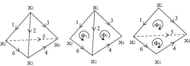
Figure 3: Patching of the faces at the tetrahedron. The vector symbol ${\vec{\ell}}$ is omitted at the edges and only their label is denoted. Curly arrow shows the orientation of each faces. The sign of the vector ${\vec{\ell}}_{i}$ in $\Phi$ is determined by whether the arrow at the edge is the same (resp. opposite) direction to the curly arrow of the face which represent $\Phi$.

We put the membrane field (36) into eq.(41), the phase factor before the integration becomes (the assignment of ${\vec{\ell}}_{i}$ is written in Fig.3),

$$iC(\vec{x}^{1}_{c}\cdot({\vec{\ell}}_{1}\times{\vec{\ell}}_{2})+\vec{x}^{2}_{c}\cdot({\vec{\ell}}_{2}\times{\vec{\ell}}_{3})+\vec{x}^{3}_{c}\cdot({\vec{\ell}}_{3}\times{\vec{\ell}}_{1})+\vec{x}^{4}_{c}\cdot({\vec{\ell}}_{4}\times{\vec{\ell}}_{5}))$$

$$=iC(\vec{y}^{1}_{c}\cdot({\vec{\ell}}_{1}\times{\vec{\ell}}_{2})+\vec{y}^{2}_{c}\cdot({\vec{\ell}}_{2}\times{\vec{\ell}}_{3})+\vec{y}^{3}_{c}\cdot({\vec{\ell}}_{3}\times{\vec{\ell}}_{1})+\vec{y}^{4}_{c}\cdot({\vec{\ell}}_{4}\times{\vec{\ell}}_{5}))$$

$$~{}~{}~{}~{}~{}~{}~{}~{}~{}+iCx^{t}_{c}({\vec{\ell}}_{1}\times{\vec{\ell}}_{2}+{\vec{\ell}}_{2}\times{\vec{\ell}}_{3}+{\vec{\ell}}_{3}\times{\vec{\ell}}_{1}+{\vec{\ell}}_{4}\times{\vec{\ell}}_{5})\,,$$ (42)

where $\vec{x}^{t}_{c}=\frac{\vec{x}_{1}+\vec{x}_{2}+\vec{x}_{3}+\vec{x}_{4}}{4}$ and $\vec{y}^{i}_{c}=\vec{x}^{i}_{c}-\vec{x}^{t}_{c}$. The expression in the third line vanishes because of the momentum conservation at the vertex. On the other hand, the expression in the second line becomes

$$iC{\vec{\ell}}_{1}\cdot({\vec{\ell}}_{2}\times{\vec{\ell}}_{3})=iCV$$ (43)

where $V$ is the volume of the tetrahedron. This is the phase factor which we observed in the previous section. Since the dependence on the center of the mass coordinate $\vec{x}^{t}_{c}$ vanishes, the integration on this variable gives rise to $\delta^{(3)}(0)$ again. So it will be more useful to define the quartic product $\left<\Phi,\Phi,\Phi,\Phi\right>$ by the integration over the relative coordinates ${\vec{\ell}}_{i}$,

$$\left<\Phi_{1},\Phi_{2},\Phi_{3},\Phi_{4}\right> = \int d\vec{\ell}_{1}\cdots d\vec{\ell}_{6}\,e^{iC\vec{\ell}_{1}\cdot(\vec{\ell}_{2}\times\vec{\ell}_{3})}\,\cdot$$ (44)

$$\cdot\hat{\Phi}_{1}(\vec{\ell}_{1},\vec{\ell}_{6},-\vec{\ell}_{2})\hat{\Phi}_{2}(\vec{\ell}_{2},\vec{\ell}_{4},-\vec{\ell}_{3})\hat{\Phi}_{3}(-\vec{\ell}_{1},\vec{\ell}_{3},\vec{\ell}_{5})\hat{\Phi}_{4}(-\vec{\ell}_{4},-\vec{\ell}_{6},-\vec{\ell}_{5})\cdot$$

$$\cdot\,\delta^{(3)}(\vec{\ell}_{1}+\vec{\ell}_{6},-\vec{\ell}_{2})\delta^{(3)}(\vec{\ell}_{2}+\vec{\ell}_{4}-\vec{\ell}_{3})\delta^{(3)}(-\vec{\ell}_{1}+\vec{\ell}_{3}+\vec{\ell}_{5})\,.$$

In the next section, we introduce the interaction term for the tachyon field by using this product. As in the inner product, we need to be careful in choosing the normalization. We postpone this issue to the next section since it is more complicated.

Since the quartic product defines a map ${\cal H}^{\otimes 4}\rightarrow\mathbf{C}$, we can obtain a triplet product $[\Phi,\Phi,\Phi]$ ${\cal H}^{\otimes 3}\rightarrow\mathcal{H}$ by conjugation with respect to one membrane field, namely by requiring

$$\left<\Phi_{1},\Phi_{2},\Phi_{3},\Phi_{4}\right>=([\Phi_{1},\Phi_{2},\Phi_{3}],\Phi_{4}).$$ (45)

In terms of the $\vec{x}$ representation,

$$[\Phi_{1},\Phi_{2},\Phi_{3}](\vec{x}_{1},\vec{x}_{2},\vec{x}_{3})=\int d^{3}\vec{x}\,\Phi_{1}(\vec{x},\vec{x}_{2},\vec{x}_{1})\Phi_{2}(\vec{x},\vec{x}_{3},\vec{x}_{2})\Phi_{3}(\vec{x},\vec{x}_{1},\vec{x}_{3}).$$ (46)

This is the natural definition of the triplet product for truncated open membranes. It is obviously different from the triplet product we defined for the ground states. But we will see below that, restricting the truncated open membrane to ground states in the $C$-field background, this triplet product (46) reduces to exactly the same product (49) for ground states.

The Fourier transform of the product $[\Phi_{1},\Phi_{2},\Phi_{3}]$ is given by

$$\widetilde{[\Phi_{1},\Phi_{2},\Phi_{3}]}(\vec{k};\vec{\ell}_{1},\vec{\ell}_{2},-{\vec{\ell}}_{1}-{\vec{\ell}}_{2})=\int d^{3}\vec{k}_{1}d^{3}\vec{k}_{3}d^{3}\vec{\ell}\;e^{\frac{i}{3}(\vec{k}\cdot\vec{\ell}+\vec{k}_{1}\cdot\vec{\ell}_{2}-\vec{k}_{3}\cdot\vec{\ell}_{1})}{\tilde{\Phi}_{1}}(\vec{k}_{1};-\vec{\ell},\vec{\ell}-\vec{\ell}_{1},{\vec{\ell}}_{1})$$

$${\tilde{\Phi}_{2}}(\vec{k}-\vec{k}_{1}-\vec{k}_{3};\vec{\ell}_{1}-\vec{\ell},\vec{\ell}+\vec{\ell}_{2},-{\vec{\ell}}_{1}-{\vec{\ell}}_{2}){\tilde{\Phi}_{3}}(\vec{k}_{3};-\vec{\ell}-\vec{\ell}_{2},\vec{\ell},{\vec{\ell}}_{2}).$$ (47)

From this, we can write the on-shell part of the triplet product as

$$\widetilde{[\Phi_{1},\Phi_{2},\Phi_{3}]}(\vec{k};\vec{\ell}_{1},\vec{\ell}_{2},-{\vec{\ell}}_{1}-{\vec{\ell}}_{2})\equiv\delta^{(3)}(\vec{k}-C\vec{\ell}_{1}\times\vec{\ell}_{2})\widehat{[\Phi_{1},\Phi_{2},\Phi_{3}]}(\vec{\ell}_{1},\vec{\ell}_{2},-\vec{\ell}_{1}-\vec{\ell}_{2}),$$ (48)

$$\widehat{\left[\Phi_{1},\Phi_{2},\Phi_{3}\right]}(\vec{\ell}_{1},\vec{\ell}_{2},-{\vec{\ell}}_{1}-{\vec{\ell}}_{2})$$

$$~{}~{}~{}~{}~{}=\int d\vec{\ell}\,e^{iC\vec{\ell}\cdot(\vec{\ell}_{1}\times\vec{\ell}_{2})}\hat{\Phi}_{1}(-\vec{\ell},\vec{\ell}-\vec{\ell}_{1},{\vec{\ell}}_{1})\hat{\Phi}_{2}(\vec{\ell}_{1}-\vec{\ell},\vec{\ell}+\vec{\ell}_{2},-{\vec{\ell}}_{1}-{\vec{\ell}}_{2})\hat{\Phi}_{3}(-\vec{\ell}-\vec{\ell}_{2},\vec{\ell},{\vec{\ell}}_{2})\,.$$ (49)

5 Scalar field theory on nonassociative space

Let us consider an analogy of the scalar field theory for the membrane field. The dimensions of the spacetime should be taken as a multiple of $3$. We will just consider the case of 3-dimensions here for simplicity. While it is possible to include the complicated interaction terms which can be constructed by using various product formula in Sec. 8 below, we first examine the simplest action for the membrane field $\Phi(\vec{k})$

$$S = S_{kin}-S_{int}\,,$$ (50)

where the first term is the ordinary kinetic term

$$S_{kin}=\int d^{3}\vec{k}\Psi^{\ast}(\vec{k})(\vec{k}^{2}+m^{2})\Psi(\vec{k}),$$ (51)

and the second term is the 4-point interaction vertex obtained in the previous section

$$S_{int}=\frac{g}{4!}\int d^{3}\vec{k}_{1}d^{3}\vec{k}_{2}d^{3}\vec{k}_{3}\cos\left(C^{-1/2}\sqrt{|\vec{k}_{1}\cdot(\vec{k}_{2}\times\vec{k}_{3})|}\right)\Psi(\vec{k}_{1})\Psi(\vec{k}_{2})\Psi(\vec{k}_{3})\Psi(-\vec{k}_{1}-\vec{k}_{2}-\vec{k}_{3}).$$ (52)

One may feel a bit unease with the absolute value involved in the definition of $S_{int}$, and in view of the notion of truncated open membrane which we introduced above, it is worthwhile to construct an equivalent description of the field theory in terms of the wave functions $\Phi(\vec{\ell}_{1},\vec{\ell}_{2},\vec{\ell}_{3})$ labeled by $\vec{\ell}$’s. Since the only quantum number of the open membrane ground state is the momentum, if we denote the ground state with momentum $\vec{k}$ by $|\vec{k}\rangle$, a generic wave function for the ground state is

$$|\Phi\rangle=\int d^{3}\vec{k}\Psi(\vec{k})|\vec{k}\rangle.$$ (53)

On the other hand, in terms of the wave function $\Phi(\vec{\ell}_{1},\vec{\ell}_{2},\vec{\ell}_{3})$, it should be

$$|\Phi\rangle=\int d^{3}\vec{\ell}_{1}d^{3}\vec{\ell}_{2}\Phi(\vec{\ell}_{1},\vec{\ell}_{2},-\vec{\ell}_{1}-\vec{\ell}_{2})|C\vec{\ell}_{1}\times\vec{\ell}_{2}\rangle.$$ (54)

The connection between these two representations is therefore

$$\Psi(\vec{k})=\int d^{3}\vec{\ell}_{1}d^{3}\vec{\ell}_{2}\delta^{(3)}(\vec{k}-C\vec{\ell}_{1}\times\vec{\ell}_{2})\Phi(\vec{\ell}_{1},\vec{\ell}_{2},-\vec{\ell}_{1}-\vec{\ell}_{2}).$$ (55)

In terms of $\Phi(\vec{\ell}_{1},\vec{\ell}_{2},\vec{\ell}_{3})$, the kinetic term of the action is

$$S_{kin} = \frac{1}{2}\int d^{3}\vec{\ell}_{1}d^{3}\vec{\ell}_{2}d^{3}\vec{\ell}^{\prime}_{1}d^{3}\vec{\ell}^{\prime}_{2}\;\Phi^{\ast}(\vec{\ell}_{1},\vec{\ell}_{2},-\vec{\ell}_{1}-\vec{\ell}_{2})\left(C^{2}(\vec{\ell}_{1}\times\vec{\ell}_{2})^{2}+m^{2}\right)\cdot$$ (56)

$$~{}~{}~{}~{}~{}\cdot\Phi(\vec{\ell}^{\prime}_{1},\vec{\ell}^{\prime}_{2},-\vec{\ell}^{\prime}_{1}-\vec{\ell}^{\prime}_{2})\,\delta^{(3)}(\vec{\ell}_{1}\times\vec{\ell}_{2}-\vec{\ell}^{\prime}_{1}\times\vec{\ell}^{\prime}_{2})\,.$$

The interaction term is

$$S_{int} = \int d^{3}\vec{\ell}_{1}d^{3}\vec{\ell}_{2}d^{3}\vec{\ell}_{3}\,{\cal N}(\vec{\ell})\,e^{iC\vec{\ell}_{1}\cdot(\vec{\ell}_{2}\times\vec{\ell}_{3})}\,\Phi(\vec{\ell}_{1}-\vec{\ell}_{2},-\vec{\ell}_{1},\vec{\ell}_{2})\Phi(-\vec{\ell}_{2},\vec{\ell}_{3},\vec{\ell}_{2}-\vec{\ell}_{3})\,\cdot$$ (57)

$$\Phi(-\vec{\ell}_{3},\vec{\ell}_{1},\vec{\ell}_{3}-\vec{\ell}_{1})\Phi(\vec{\ell}_{3}-\vec{\ell}_{2},\vec{\ell}_{1}-\vec{\ell}_{3},\vec{\ell}_{2}-\vec{\ell}_{1})\,,$$

where $\vec{\ell}_{1},\vec{\ell}_{2},\vec{\ell}_{3}$ spans a tetrahedron whose faces match with the arguments of the 4 $\Phi$’s. The normalization factor ${\cal N}(\vec{\ell})$ will be determined later.

The kinetic term (56) looks a bit complicated. One may wonder what happens if we make a more naive choice

$$S^{\prime}_{kin}(\Phi)=\frac{1}{2}\int d^{9}\vec{\ell}\;\delta^{(3)}({\vec{\ell}}_{1}+{\vec{\ell}}_{2}+{\vec{\ell}}_{3})\Phi^{\ast}({\vec{\ell}}_{1},{\vec{\ell}}_{2},{\vec{\ell}}_{3})\left(C^{2}(\vec{\ell}_{1}\times\vec{\ell}_{2})^{2}+m^{2}\right)\Phi({\vec{\ell}}_{1},{\vec{\ell}}_{2},{\vec{\ell}}_{3})\,.$$ (58)

It implies a propagator of the form

$$\langle\Phi({\vec{\ell}}^{\prime})\Phi({\vec{\ell}})\rangle^{\prime}=\frac{1}{C^{2}(\vec{\ell}_{1}\times\vec{\ell}_{2})^{2}+m^{2}}\delta^{(3)}({\vec{\ell}}+{\vec{\ell}}^{\prime})\,.$$ (59)

However, this definition leads to a Feynman rule which is very restrictive. For example, the internal loop momentum of the one-loop diagram in figure 4 (b) is completely fixed by the external legs. Furthermore, the external legs on the left must have exactly the same labels $\vec{\ell}$ as the other two external legs on the right. This is a result of the fact that the labels $\vec{\ell}$ on any two faces of a tetrahedron completely fix the labels on the other two faces, and the fact that this propagator does not connect cross sections with different shapes.

5.1 Feynman diagrams

In this section we consider basic Feynman diagrams involving the 4-membrane interaction vertex $[\Phi,\Phi,\Phi,\Phi]^{(4)}$.

Before we start computing Feynman diagrams, we need to understand the phase space. For particles with no internal degrees of freedom, the state of a free particle can be specified by its momentum $p$. For the triangular open membrane, its internal degrees of freedom are parameterized by two 3-vectors ($\vec{\ell}_{1}$, $\vec{\ell}_{2}$) constrained by

$$\vec{p}=C\vec{\ell}_{1}\times\vec{\ell}_{2}$$ (60)

for the state with momentum $\vec{p}$. Hence the phase space for the internal degrees of freedom has the measure

$$d^{3}\vec{\ell}_{1}\;d^{3}\vec{\ell}_{2}\;\delta^{(3)}(\vec{p}-C\vec{\ell}_{1}\times\vec{\ell}_{2}).$$ (61)

As $\vec{p}$ and $\vec{\ell}_{1}$ are always perpendicular to each other, we can use $\vec{p}$, $\vec{\ell}_{1}$ and $\vec{p}\times\vec{\ell}_{1}$ as an orthogonal basis of vectors and expand $\vec{\ell}_{2}$ as

$$\vec{\ell}_{2}=a\vec{p}\times\vec{\ell}_{1}+b\vec{\ell}_{1}+c\vec{p}.$$ (62)

Then

$$d^{3}\vec{\ell}_{2}=da\;db\;dc\;(\vec{p}\times\vec{\ell}_{1})^{2}$$ (63)

and the measure (61) can be simplified as

$$d^{3}\vec{\ell}_{1}\;db\;\frac{1}{C^{2}}\delta(\vec{p}\cdot\vec{\ell}_{1}),$$ (64)

while $\vec{\ell}_{2}$ is now fixed to be

$$\vec{\ell}_{2}=\frac{1}{C\ell_{1}^{2}}(\vec{p}\times\vec{\ell}_{1})+b\vec{\ell}_{1}.$$ (65)

5.1.1 Tree diagram

Let us consider the tree level diagram of 4 external legs with a single interaction vertex. For the 4 membranes to fit onto the 4 edges of a tetrahedron defined by $(\vec{\ell}_{1},\vec{\ell}_{2},\vec{\ell}_{3})$, the external legs must have triangular cross sections given by $(\vec{\ell}_{1},\vec{\ell}_{2})$, $(\vec{\ell}_{2},\vec{\ell}_{3})$, $(\vec{\ell}_{3},\vec{\ell}_{1})$ and $(\vec{\ell}_{1}-\vec{\ell}_{2},\vec{\ell}_{3}-\vec{\ell}_{2})$.

For given momenta of the external legs $\vec{p}_{i}$ $(i=1,2,3,4)$, the tree level diagram which is simply the 4-membrane vertex is supposed to be given by

$$\cos\left(C^{-1/2}\sqrt{|\vec{p}_{1}\cdot(\vec{p}_{2}\times\vec{p}_{3})|}\right),$$ (66)

where the sign is determined by the orientation of the tetrahedron. We would like to see how this can be derived from integration over the phase space of internal degrees of freedom. The 4-membrane vertex is

$${\cal A}_{0} = \int d^{3}\vec{\ell}_{1}d^{3}\vec{\ell}_{2}d^{3}\vec{\ell}_{3}\,{\cal N}(\vec{\ell})\,\delta^{(3)}(\vec{p}_{1}-C\vec{\ell}_{1}\times\vec{\ell}_{2})\;\delta^{(3)}(\vec{p}_{2}-C\vec{\ell}_{2}\times\vec{\ell}_{3})\;\delta^{(3)}(\vec{p}_{3}-C\vec{\ell}_{3}\times\vec{\ell}_{1})\cdot$$ (67)

$$\delta^{(3)}\left(\vec{p}_{4}-C(\vec{\ell}_{1}-\vec{\ell}_{2})\times(\vec{\ell}_{3}-\vec{\ell}_{2})\right)\;e^{iC\vec{\ell}_{1}\cdot(\vec{\ell}_{2}\times\vec{\ell}_{3})},$$

where we have introduced a normalization factor ${\cal N}$. Carrying out the integration over $\vec{\ell}_{i}$’s, we find

$${\cal A}_{0}=\delta^{(3)}(\vec{p}_{1}+\vec{p}_{2}+\vec{p}_{3}+\vec{p}_{4})\;{\cal M}_{0},$$ (68)

where

$${\cal M}_{0}=2\cos(C^{-1/2}\sqrt{|\vec{p}_{1}\cdot(\vec{p}_{2}\times\vec{p}_{3})|})\;\frac{{\cal N}(\vec{\ell})}{C^{9/2}|\vec{p}_{1}\cdot(\vec{p}_{2}\times\vec{p}_{3})|^{3/2}}.$$ (69)

It follows that we should choose

$${\cal N}(\vec{\ell})\equiv C^{9}|\vec{\ell}_{1}\cdot(\vec{\ell}_{2}\times\vec{\ell}_{3})|^{3}=C^{9/2}|\vec{p}_{1}\cdot(\vec{p}_{2}\times\vec{p}_{3})|^{3/2}\equiv{\cal N}(\vec{p}),$$ (70)

so that (69) is just the sum over the interaction vertex (66) for the two possible orientations of the tetrahedron.

$\begin{array}[]{ccc}\begin{picture}(40.0,30.0)(-20.0,-15.0)\put(0.0,0.0){\circle{40.0}} \put(-15.0,-6.8){\line(1,0){30.0}} \put(-13.0,-10.0){$\vec{p}$} \put(13.0,-10.0){$\vec{p}$} \put(0.0,8.0){$\vec{q}$} \end{picture}&\begin{picture}(40.0,30.0)(-20.0,-15.0)\put(0.0,0.0){\circle{40.0}} \put(-16.8,10.0){\vector(1,-1){10.0}} \put(-16.8,-10.0){\vector(1,1){10.0}} \put(6.8,0.0){\vector(1,1){10.0}} \put(6.8,0.0){\vector(1,-1){10.0}} \put(-16.0,5.0){$\vec{p}_{1}$} \put(-16.0,-5.0){$\vec{p}_{2}$} \put(14.0,5.0){$\vec{p}_{3}$} \put(14.0,-5.0){$\vec{p}_{4}$} \end{picture}&\begin{picture}(40.0,30.0)(-20.0,-15.0)\put(-15.0,0.0){\vector(1,0){30.0}} \put(0.0,0.0){\circle{40.0}} \put(-12.0,2.0){$\vec{p}$} \put(10.0,2.0){$\vec{p}$} \end{picture}\\ \mbox{(a)}&\mbox{(b)}&\mbox{(c)}\end{array}$

Figure 4: (a) The 1-loop diagram corresponding to eq. (71). (b) The 1-loop diagram corresponding to eq. (73) (c) The 2-loop diagram corresponding to eq. (74).

5.1.2 One-loop diagram

The 1-loop diagram in Fig. (4) (a) is not modified by the phase factor depending on $C$ because two of the momenta of the 4-membrane interaction vertex is the same vector, and the volume of the tetrahedron must be zero. This diagram is thus exactly the same as in usual field theory

$${\cal M}_{1}=\int d^{3}\vec{p}\frac{1}{\vec{p}^{2}+m^{2}}.$$ (71)

Another 1-loop diagram, the one in Fig (4) (b), is less trivial. It is

$${\cal A}^{\prime}_{1} = \int\prod_{i=1}^{6}d^{3}\vec{\ell}_{i}\;d^{3}\vec{p}\;d^{3}\vec{q}\;\delta^{(3)}(\vec{p}_{1}-C\vec{\ell}_{2}\times\vec{\ell}_{1})\;\delta^{(3)}(\vec{p}_{2}-C\vec{\ell}_{3}\times\vec{\ell}_{2})\;\delta^{(3)}(\vec{p}-C\vec{\ell}_{5}\times\vec{\ell}_{4})\;\delta^{(3)}(\vec{q}-C\vec{\ell}_{6}\times\vec{\ell}_{5})\cdot$$ (72)

$$\delta^{(3)}(\vec{p}-C\vec{\ell}_{3}\times\vec{\ell}_{1})\;\delta^{(3)}(\vec{q}-C\vec{\ell}_{1}\times\vec{\ell}_{2})\;\delta^{(3)}(\vec{p}_{3}-C\vec{\ell}_{6}\times\vec{\ell}_{4})\;\delta^{(3)}(\vec{p}_{4}-C(\vec{\ell}_{4}-\vec{\ell}_{5})\times(\vec{\ell}_{6}-\vec{\ell}_{5}))\cdot$$

$$\frac{1}{\vec{p}^{2}+m^{2}}\frac{1}{\vec{q}^{2}+m^{2}}\;{\cal N}(\vec{p}_{1},\vec{p}_{2},\vec{p})\;{\cal N}(\vec{p}_{3},\vec{p}_{4},\vec{p})\;e^{iC\vec{\ell}_{1}\cdot(\vec{\ell}_{2}\times\vec{\ell}_{3})}\;e^{iC\vec{\ell}_{4}\cdot(\vec{\ell}_{5}\times\vec{\ell}_{6})},$$

where ${\cal N}(\vec{p}_{1},\vec{p}_{2},\vec{p})$ is defined in (70). It is straightforward to find, up to the delta function imposing momentum conservation, the amplitude ${\cal A}^{\prime}_{1}$ is, up to the delta function imposing energy-momentum conservation,

$${\cal M}^{\prime}_{1}=\int d^{3}\vec{p}\;\frac{1}{\vec{p}^{2}+m^{2}}\frac{1}{(\vec{p}_{1}+\vec{p}_{2}-\vec{p})^{2}+m^{2}}2\cos(C^{-1/2}\sqrt{|\vec{p}\cdot(\vec{p}_{1}\times\vec{p}_{2})|})2\cos(C^{-1/2}\sqrt{|\vec{p}\cdot(\vec{p}_{3}\times\vec{p}_{4})|}).$$ (73)

Generically (if $\vec{p}_{1}\times\vec{p}_{2}$ and $\vec{p}_{3}\times\vec{p}_{4}$ are not parallel), $\vec{p}$ has an effective cutoff in two directions due to the two $\cos$ factors. The integral is obviously finite.

If the spacetime dimension is 6, we replace the momenta by 6-vectors. We would then have another two $\cos$ factors due to the nonassociativity in the other 3 dimensions. The 6 dimensional integral of $\vec{p}$ is unbounded only in 2 directions, and thus the integral is finite. The diagram has a logrithmic divergence in 12 dimensions.

5.1.3 2-loop diagram

The 2-loop diagram in Fig. 4 (c) can be obtained from Fig. 4 (b) by identifying $\vec{p}_{2}$ with $\vec{p}_{3}$ and integrating over $\vec{p}_{2}$. Therefore

$${\cal M}_{2}=\int d^{3}\vec{p}^{\prime}\;d^{3}\vec{q}\;\frac{1}{\vec{p}^{\prime}{}^{2}+m^{2}}\frac{1}{\vec{q}^{2}+m^{2}}\frac{1}{(\vec{p}-\vec{p}^{\prime}-\vec{q})^{2}+m^{2}}4\cos^{2}(C^{-1/2}\sqrt{|\vec{p}\cdot(\vec{p}^{\prime}\times\vec{q})|}).$$ (74)

The cosine factor imposes an effective cutoff at the energy scale

$$\Lambda_{\mbox{eff}}=\sqrt{\frac{C}{|p|}}\,.$$ (75)

As a result the integral is finite, although it would have a logrithmic divergence without the cosine factor.

The diagram diverges if the spacetime dimension is 6 or higher.

We suspect that there is no real divergence which can not be removed by normal ordering in this scalar field theory living on a 3 dimensional nonassociative space. (The divergence of ${\cal M}_{1}$ in (71) can be removed by normal ordering.)

6 Inclusion of internal degree of freedom

In the above we have considered open membranes ending on a single M5-brane. For a stack of $N$ M5-branes, open membranes should acquire internal degrees of freedom analogous to Chan-Paton factors. Naively, there are cylindrical membranes stretched between 2 M5-branes, just like open strings stretched between 2 D-branes, and so one expects a non-Abelian gauge theory on the M5-brane world-volume at low energy. However, anomaly and entropy computations [35] suggest that the world-volume theory has $N^{3}$ degrees of freedom, rather than $N^{2}$ as in Yang-Mills theory. Interestingly, $N^{3}$ is precisely what our truncated model of open membrane would suggest. For the triangular membrane, it is natural to introduce Chan-Paton factors either on the corners or on the edges. The Chan-Paton factors on the corners are easily incorporated in our formulation above, since it is simply the extension of the coordinates $\vec{x}_{i}$ ($i=1,2,3$) to include additional indices $(\vec{x}_{i},n_{i})$ $(i=1,2,3)$. Hence we will only discuss other less trivial ways of introducing internal degrees of freedom.

First we present a prescription [33, 34] which was originally proposed as a generalization of the matrix model whose Feynman rule produces the 3d gravity and fit with our formulation. It corresponds to open membranes with boundaries divided into 3 sections belonging to 3 M5-branes.

We introduce three indices to each wave function assigned with a triangle,

$$\Phi({\vec{\ell}})\quad\rightarrow\quad\Phi_{ijk}({\vec{\ell}})$$ (76)

where the indices $i,j,k$ take values from $1,\cdots,N$. We may assign the symmetry under the permutation of indices. For example, a natural generalization of the Hermitian matrix is

$$\mathrm{Re}(\Phi_{i_{\sigma(1)}i_{\sigma(2)}i_{\sigma(3)}})=\mathrm{Re}(\Phi_{i_{1}i_{2}i_{3}})\,,\quad\mathrm{Im}(\Phi_{i_{\sigma(1)}i_{\sigma(2)}i_{\sigma(3)}})=(-1)^{\sigma}\mathrm{Im}(\Phi_{i_{1}i_{2}i_{3}})\,,\quad\sigma\in S_{3}\,.$$ (77)

In either case, we assume that $\Phi_{ijk}$ is invariant under the cyclic permutation of $i,j,k$.

We may attach the three indices to the three edges of the triangle. At the vertex, as our ${\vec{\ell}}$, we put the four field $\Phi^{(a)}$ at the faces of a tetrahedron and identify the indices which share the same edge and sum over them. More explicitly we have,

$$\left<\!\!\left<\Phi^{(1)},\Phi^{(2)},\Phi^{(3)},\Phi^{(4)}\right>\!\!\right>=\sum_{i_{1}\cdots i_{6}=1}^{N}\left<\Phi^{(1)}_{i_{1},i_{2},i_{6}},\Phi^{(2)}_{i_{2},i_{3},i_{4}},\Phi^{(3)}_{i_{3},i_{1},i_{5}},\Phi^{(4)}_{i_{4},i_{5},i_{6}}\right>,$$ (78)

where the single bracket $\left<\Phi,\Phi,\Phi,\Phi\right>$ is the quartic product (44) which was defined by the integral over ${\vec{\ell}}$. The connections of colors at the vertex is the same as figure 3. Similarly, the triplet product should be defined as

$$\left[\!\!\left[\Phi^{(1)},\Phi^{(2)},\Phi^{(3)}\right]\!\!\right]_{i_{4},i_{5},i_{6}}=\sum_{i_{1}\cdots i_{3}=1}^{N}\left[\Phi^{(1)}_{i_{1},i_{2},i_{6}},\Phi^{(2)}_{i_{2},i_{3},i_{4}},\Phi^{(3)}_{i_{3},i_{1},i_{5}}\right].$$ (79)

By writing three lines along each propagator and the connections of these lines at the vertices, one can write a fat graph associated with a given Feynman diagram. As an example, in fig. 5, we give two types of the fat graphs associated with the Feynman graph fig. 4b. As the diagrams of usual gauge theories, one obtains the factor of $N$ for each loop of the index line. Since one may use twist $\sigma\in S_{3}$ for the propagator, there are a few different fat graphs associated with a single Feynman diagram and each graph may have different dependence on $N$. In the fig. 5, the left graph has factor $N$ from the index loop. On the other hand, the right graph does not have that factor and is $O(1)$. This is very similar to the computation of the gauge theory. For the gauge theory, if we forget the dependence on $x$, the system is reduced to the matrix model. The dual diagram of the fat graph corresponds to the triangulation of the 2d surface. A similar phenomena happens in our case too. If we forget the ${\vec{\ell}}$ dependence, the Feynman integral reduces to the integration over the cubic matrix $\Phi_{ijk}$. We can associate each vertex an tetrahedron and the propagator indicates how two tetrahedra are connected at the faces. In this way, the dual diagram to each fat graph gives a symplicial decomposition of the 3d space. In [34], it was shown that the two parameters $g$ and $N$ are identified with the Newton’s constant and the consmological constant. In the 3d case, however, there is the difficulty that the dual graph for the Feynman graph may not define a manifold. So the correspondence between the Feynman graphs and the lattice gravity is not so clear as the 2d case.

Figure 5: Two fat graphs associated with Feynman graph Fig.4(b)

Other possibilities

Here we examine a few more ideas to introduce the internal degree of freedom. One such possibility is to consider an analog of the noncommutative torus with the rational $\theta$ parameter. It is equivalent to the matrix algebra. We recall that the basis of $N\times N$ matrix is spanned by the matrices $U^{n_{1}}V^{n_{2}}$ ($n_{1},n_{2}\in\mathbf{Z}_{N}$) where $U,V$ satisfies $UV=VUe^{2\pi i/N}$. It is then easy to see that

$$(U^{n_{1}}V^{n_{2}})(U^{m_{1}}V^{m_{2}})=e^{-\frac{2\pi i}{N}(n_{1}m_{2}-m_{1}n_{2})}(U^{m_{1}}V^{m_{2}})(U^{n_{1}}V^{n_{2}})\,.$$ (80)

Therefore the matrix algebra is expressed as the noncommutative phase $(n_{1},m_{1};n_{2},m_{2})\rightarrow e^{\frac{2\pi i}{N}(n_{1}m_{2}-m_{1}n_{2})}$.

One may generalize this idea to three dimensions. We extend $\mathbf{R}^{3}$ to the product space $\mathbf{R}^{3}\times\mathbf{Z}_{N}^{\otimes 3}$, i.e., we require that the field $\Phi$ depends on these extra “dimensions” $\Phi({\vec{\ell}}_{1},{\vec{\ell}}_{2},{\vec{\ell}}_{3};{\vec{n}}_{1},{\vec{n}}_{2},{\vec{n}}_{3})$ (${\vec{n}}_{i}\in\mathbf{Z}_{N}^{\otimes 3}$, ${\vec{n}}_{1}+{\vec{n}}_{2}+{\vec{n}}_{3}\equiv 0$ mod $N$). The quartic product is then defined as (after neglecting degree of freedom of ${\vec{\ell}}$)

$$\left<\Phi^{(1)},\Phi^{(2)},\Phi^{(3)},\Phi^{(4)}\right> = \sum_{{\vec{n}}_{1}\cdots{\vec{n}}_{6}\in\mathbf{Z}_{N}}\,e^{\frac{2\pi i}{N}{\vec{n}}_{1}\cdot({\vec{n}}_{2}\times{\vec{n}}_{3})}\,\cdot$$ (81)

$$\cdot\hat{\Phi}^{(1)}({\vec{n}}_{1},{\vec{n}}_{6},-{\vec{n}}_{2})\hat{\Phi}^{(2)}({\vec{n}}_{2},{\vec{n}}_{4},-{\vec{n}}_{3})\hat{\Phi}^{(3)}(-{\vec{n}}_{1},{\vec{n}}_{3},{\vec{n}}_{5})\hat{\Phi}^{(4)}(-{\vec{n}}_{4},-{\vec{n}}_{6},-{\vec{n}}_{5})\cdot$$

$$\cdot\,\delta^{(3)}({\vec{n}}_{1}+{\vec{n}}_{6}-{\vec{n}}_{2})\delta^{(3)}({\vec{n}}_{2}+{\vec{n}}_{4}-{\vec{n}}_{3})\delta^{(3)}(-{\vec{n}}_{1}+{\vec{n}}_{3}+{\vec{n}}_{5})\,.$$

As in the relation between $\vec{p}$ and ${\vec{\ell}}$, the “ground state” wave function may depends only on $\lambda={\vec{n}}_{1}\times{\vec{n}}_{2}$,

$$\Phi({\vec{n}}_{1},{\vec{n}}_{2},{\vec{n}}_{3})=\psi({\vec{n}}_{1}\times{\vec{n}}_{2})\,.$$ (82)

In this case, the quartic product $[\Phi^{(1)},\Phi^{(2)},\Phi^{(3)},\Phi^{(4)}]^{(4)}$ is simplified to,

$$\sum_{{\vec{\lambda}}_{1},\cdots,{\vec{\lambda}}_{4}\in\mathbf{Z}_{N}}W({\vec{\lambda}})\delta(\sum_{i=1}^{4}{\vec{\lambda}}_{i})\cos\left({\frac{2\pi}{N}\sqrt{|{\vec{\lambda}}_{1}\cdot({\vec{\lambda}}_{2}\times{\vec{\lambda}}_{3})|}}\right)\psi_{1}({\vec{\lambda}}_{1})\psi_{2}({\vec{\lambda}}_{2})\psi_{3}({\vec{\lambda}}_{3})\psi_{4}({\vec{\lambda}}_{4}),$$ (83)

where

$$W({\vec{\lambda}}) = \sum_{{\vec{n}}_{1}\cdots{\vec{n}}_{6}\in\mathbf{Z}_{N}}\delta({\vec{\lambda}}_{1}-{\vec{n}}_{1}\times{\vec{n}}_{2})\delta({\vec{\lambda}}_{2}-{\vec{n}}_{2}\times{\vec{n}}_{3})\delta({\vec{\lambda}}_{3}-{\vec{n}}_{3}\times{\vec{n}}_{1})\delta(\sum_{i=1}^{3}{\vec{\lambda}}_{i}-{\vec{n}}_{4}\times{\vec{n}}_{5})\cdot$$ (84)

$$\cdot\delta^{(3)}({\vec{n}}_{1}+{\vec{n}}_{6}-{\vec{n}}_{2})\delta^{(3)}({\vec{n}}_{2}+{\vec{n}}_{4}-{\vec{n}}_{3})\delta^{(3)}(-{\vec{n}}_{1}+{\vec{n}}_{3}+{\vec{n}}_{5})\,.$$

is the non-negative integer weight for ${\vec{\lambda}}$. When the square root phase factor $\sqrt{|{\vec{\lambda}}_{1}\cdot({\vec{\lambda}}_{2}\times{\vec{\lambda}}_{3})|}$ becomes non-integer for generic $\lambda$, this weight factor vanishes. Unlike the two dimensional case, this assignment of the internal degree of freedom is not equivalent to the previous one.

7 Some generalization of membrane fields and their interactions

In this paper, we concentrate ourselves to the membrane field which is represented by a triangle. This restriction is chosen in order to obtain the simplest toy model to describe the basic feature of the membrane theory.

It is, however, obvious that the membranes can take arbitrary shape even if we restrict them to the plane perpendicular to the momentum. It implies that we miss most of the interactions except for the simplest one. If we allow them to take arbitrary shape, however, we would not be able to escape from the instability. So as the next approximation, one may have milder restriction to the shape of the membrane to the polygons. The membrane field associated with $n$-polygon $\Delta$ is written as a function of its $n$ vertices as $\Phi(\vec{x}(\Delta))$ where we introduced a shorthand notation, $x(\Delta)=(\vec{x}_{1},\cdots,\vec{x}_{n})$. We assume that $n$ vectors $\vec{x}_{1},\cdots,\vec{x}_{n}$ are located on the same plane. As before, we need to require that the momentum is proportional to the area vector,

$$\vec{p}-C\vec{A}(\Delta)=0\,,\quad\vec{A}(\Delta)=\frac{1}{2}\sum_{1\leq i<j\leq n}{\vec{\ell}}_{i}\times{\vec{\ell}}_{j}\,,$$ (85)

where ${\vec{\ell}}_{i}=\vec{x}_{i+1}-\vec{x}_{i}$, ($\vec{x}_{n+1}\equiv\vec{x}_{1}$). In terms of the membrane field, we can write it as

$$\tilde{\Phi}(\vec{p};{\vec{\ell}}(\Delta))=\hat{\Phi}({\vec{\ell}}(\Delta))\delta^{(3)}(\vec{p}-C\vec{A}(\Delta))$$ (86)

where $\tilde{\Phi}(\vec{p};{\vec{\ell}}(\Delta))$ is the Fourier transformation of $\Phi(\vec{x}(\Delta))$,

$$\tilde{\Phi}(\vec{p};{\vec{\ell}}(\Delta))=\int d\vec{x}_{c}^{\Delta}e^{i\vec{p}\cdot\vec{x}_{c}^{\Delta}}\hat{\Phi}(\vec{x}(\Delta))\,,\quad\vec{x}_{c}^{\Delta}=\frac{1}{n}\sum_{i=1}^{n}\vec{x}_{i}\,,\quad{\vec{\ell}}(\Delta)=({\vec{\ell}}_{1},\cdots,{\vec{\ell}}_{n})\,.$$ (87)

Here we need to change the variables from $\vec{x}_{i}$ to $\vec{p}$ and ${\vec{\ell}}_{i}$. The ground state of the membrane field is described by the wave function whose $\hat{\Phi}$ depends only on the momentum (or the area vector),

$$\hat{\Phi}({\vec{\ell}}(\Delta))=\phi(\vec{p})=\phi(C\vec{A}(\Delta))\,.$$ (88)

The interaction among the generalized membrane fields can be defined as before. We introduce a three dimensional open space $B$ (which may not necessarily have the topology of ball) whose boundary $\partial B$ is covered by polygons $\Delta_{f}$ ($f=1,\cdots,b_{2}$), $\partial B=\cup_{f}\Delta_{f}$. We write the number of edges and vertices of $\partial B$ as $b_{1}$ and $b_{0}$ respectively. The membrane vertex associated with $B$ is then written as

$$\left<\Phi_{1},\cdots,\Phi_{b_{2}}\right>_{B}=\int d\vec{x}\,\Phi_{1}(\vec{x}(\Delta_{1}))\cdots\Phi_{b_{2}}(\vec{x}(\Delta_{b_{2}}))$$ (89)

where the integration is over the all vertices on $\partial B$. $\vec{x}$’s which belong to the same $\Delta$ should be located on the same plane.

In terms of the $\hat{\Phi}$ components, this product is written as

$$\delta\left(\sum_{i=1}^{b_{2}}\vec{p}_{i}\right)\int d{\vec{\ell}}\,e^{iCV(B)}\hat{\Phi}({\vec{\ell}}(\Delta_{1}))\cdots\hat{\Phi}({\vec{\ell}}(\Delta_{b_{2}})),$$ (90)

where $V(B)$ is the volume of $B$.

We note that we can add arbitrary type of the interaction vertices. So far, we do not have a general principle for how to select them. As in string field theory, we need some sort of gauge princple. This is outside of the scope of the current paper but will be the most important issue in future study.

We note that as $n\rightarrow\infty$, our membrane field is getting closer to the closed string field $\Phi[X(\sigma)]$ living on the plane determined by the momentum $\vec{p}$. In this sense, our membrane field theory has some connection with (discretized) closed string field theory [39].

We can include the color degree of freedom to the membrane field associated with the polygon similary. The simplest way is to introduce the color index $i$ ($i=1,\cdots,N$) to each edge of the polygon. For $n$-gons, we have $n$ color indices. We can assume the symmetry with respect to the cyclic permutation of these indices as before. At the vertex, since each edge is always shared by two faces, we can define the identification between two indices associated with it.

Reduction to the noncommutative field theory

As an application of the use of general membrane field, we would like to derive the noncommutative field theory from the membrane through double dimensional reduction.

We assume that a spacial direction (say $x^{3}$) is compactified as $x^{3}\sim x^{3}+2\pi R$ and every membrane wraps this direction once. We suppose the $C$ field takes the form $C_{ijk}=C\epsilon_{ijk}$ ($i,j,k=1,2,3$) as usual. Since the membrane should wrap the $3$-direction, the simplest shape it can take is the cylinder, which can be spacified by two vectors, ${\vec{\ell}}_{1}$ in $1-2$ directions and ${\vec{\ell}}_{2}=2\pi R\vec{e}_{3}$ ($\vec{e}_{3}$ is the unit vector in the $3$-direction. With this set-up, the momentum vector $\vec{p}$ should be in $1-2$ directions and the relation $\vec{p}=C{\vec{\ell}}_{1}\times{\vec{\ell}}_{2}$ becomes the standard relation for the noncommutative geometry,

$$p_{i}=B\epsilon_{ij}(\ell_{1})_{j}\,,\quad i,j=1,2\,,\quad B=2\pi RC\,.$$ (91)

The simplest interaction among such membrane fields are given by the three-point function. The topology of the interaction vertex is given by a solid torus whose boundary is the torus which is divided into three cylinders attached to the membrane fields. The volume of the solid torus is given by $\pi RC|p_{1}\times p_{2}|=\frac{1}{2}B|p_{1}\times p_{2}|$. This is the phase factor of the noncommutative field theory.

Since the cylinder has two edges, the number of color degree of freedom is two. This is consistent with the noncommutative field theory whose internal degree of freedom is given by the matrix.

8 Connection with lattice gravity

In this section we make some comments on the relation between our model with lattice quantum gravity. It appears through the consistency conditions for the products among the membrane fields.

In 2d (the noncommutative case), higher vertices can be constructed by using the star product as $\mbox{Tr}(\Phi_{1}\ast\cdots\ast\Phi_{n})$, which defines the polygon with $n$ edges. The consistency condition of the construction of such vertices is that the quantity defined above does not depend on the order of taking the star product. This is exactly the associativity condition of the star product.

For the 3d case, we have a different type of product (the triplet product) which is defined for three fields instead of two. So we need to find the consistency condition which replaces the associativity. We would like to argue that this may be identical with the consistency conditions of 3d lattice gravity. The connection with the lattice gravity seems natural since the membrane theory should contain the 3d gravity as the dynamics of the world-volume.

8.1 2d (noncommutative) case

In the noncommutative case, the field $\Phi$ depends only on one momentum $\vec{k}$. We consider the consistency condition when we compute four-point functions

$$\mbox{Tr}\left(\Phi_{1}\ast\Phi_{2}\ast\Phi_{3}\ast\Phi_{4}\right)=\int d^{4}\vec{k}\Phi_{1}(\vec{k}_{1})\ast\Phi_{2}(\vec{k}_{2})\ast\Phi_{3}(\vec{k}_{3})\ast\Phi_{4}(\vec{k}_{4})\delta(\vec{k}_{1}+\vec{k}_{2}+\vec{k}_{3}+\vec{k}_{4})\,.$$ (92)

There are two different ways to evaluate this quantity. (1) We take the star product $\Phi_{1}\ast\Phi_{2}$ and $\Phi_{3}\ast\Phi_{4}$ and take their inner product. (2) Similarly we take the star products $\Phi_{2}\ast\Phi_{3}$ and $\Phi_{4}\ast\Phi_{1}$ and take their inner product. These two computations match because of the associativity of the star product. More explicitly,

(1) $$= \int d^{4}\vec{k}d\vec{k}_{5}\Phi_{1}(\vec{k}_{1})\Phi_{2}(\vec{k}_{2})e^{i\theta\vec{k}_{1}\times\vec{k}_{2}}\delta(\vec{k}_{1}+\vec{k}_{2}+\vec{k}_{5})\cdot$$ (93)

$$~{}~{}~{}~{}~{}~{}\cdot\Phi_{3}(\vec{k}_{3})\Phi_{4}(\vec{k}_{4})e^{i\theta\vec{k}_{3}\times\vec{k}_{4}}\delta(\vec{k}_{3}+\vec{k}_{4}-\vec{k}_{5})\delta(\vec{k}_{1}+\vec{k}_{2}+\vec{k}_{3}+\vec{k}_{4})$$

$$= \int d^{4}\vec{k}d\vec{k}_{6}\Phi_{2}(\vec{k}_{2})\Phi_{3}(\vec{k}_{3})e^{i\theta\vec{k}_{2}\times\vec{k}_{3}}\delta(\vec{k}_{2}+\vec{k}_{3}+\vec{k}_{6})\cdot$$

$$~{}~{}~{}~{}~{}~{}\cdot\Phi_{4}(\vec{k}_{4})\Phi_{1}(\vec{k}_{1})e^{i\theta\vec{k}_{4}\times\vec{k}_{1}}\delta(\vec{k}_{4}+\vec{k}_{1}-\vec{k}_{6})\delta(\vec{k}_{1}+\vec{k}_{2}+\vec{k}_{3}+\vec{k}_{4})$$

$$= \mbox{(2)}\,.$$

The equality comes from the fact that the phase satisfies $e^{i\theta\vec{k}_{1}\times\vec{k}_{2}+i\theta\vec{k}_{3}\times\vec{k}_{4}}=e^{i\theta\vec{k}_{2}\times\vec{k}_{3}+i\theta\vec{k}_{4}\times\vec{k}_{1}}$ when $\sum_{i=1}^{4}\vec{k}_{i}=0$. We refer to this condition as the consistency condition for the $2\leftrightarrow 2$ move (fig.6a).

$\begin{array}[]{cc}\begin{picture}(40.0,30.0)(-5.0,-20.0)\put(15.0,10.0){\vector(-3,-2){15.0}} \put(3.0,5.0){$\vec{k}_{1}$} \put(0.0,0.0){\vector(3,-2){15.0}} \put(5.0,-7.0){$\vec{k}_{2}$} \put(30.0,0.0){\vector(-3,2){15.0}} \put(23.0,5.0){$\vec{k}_{4}$} \put(15.0,-10.0){\vector(3,2){15.0}} \put(25.0,-7.0){$\vec{k}_{3}$} \put(15.0,-10.0){\line(0,1){20.0}} \put(0.0,0.0){\line(1,0){3.0}}\put(5.0,0.0){\line(1,0){3.0}}\put(10.0,0.0){\line(1,0){3.0}}\put(15.0,0.0){\line(1,0){3.0}}\put(20.0,0.0){\line(1,0){3.0}}\put(25.0,0.0){\line(1,0){3.0}} \par\end{picture}&\begin{picture}(40.0,30.0)(-10.0,-10.0)\put(16.0,24.0){\vector(-2,-3){16.0}} \put(28.0,0.0){\vector(-1,2){12.0}} \put(22.0,12.0){$\vec{k}_{2}$} \put(4.0,12.0){$\vec{k}_{1}$} \put(0.0,0.0){\vector(1,0){28.0}} \put(14.0,-5.0){$\vec{k}_{3}$} {\color[rgb]{.50,.50,.50} \put(16.0,24.0){\vector(0,-1){16.0}} \put(12.0,12.0){$\vec{k}_{5}$} \put(0.0,0.0){\vector(2,1){16.0}} \put(7.0,5.0){$\vec{k}_{4}$} \put(28.0,0.0){\vector(-3,2){12.0}} \put(20.0,5.0){$\vec{k}_{6}$} } \end{picture}\\ \mbox{(a)}&\mbox{(b)}\end{array}$

Figure 6: (a) $2\leftrightarrow 2$ move. (b) $1\leftrightarrow 3$ move.

In this case, this condition is sufficient to make the perturbation theory consistent. In the context of two dimensional gravity, however, it is more natural to include the invariance by dividing one triangle into three. To describe it, we introduce a notation,

$$[\Phi]^{(2)}(\vec{k}_{1},\vec{k}_{2},\vec{k}_{3})=\Phi(\vec{k}_{1})e^{i\theta\vec{k}_{1}\times\vec{k}_{2}}\qquad(\vec{k}_{3}=-\vec{k}_{1}-\vec{k}_{2})\,,$$ (94)

$$([\Phi_{1}]^{(2)},[\Phi_{2}]^{(2)},[\Phi_{3}]^{(2)})=\int d\vec{k}_{1}\cdots d\vec{k}_{6}[\Phi_{1}]^{(2)}(\vec{k}_{1},\vec{k}_{4},-\vec{k}_{5})[\Phi_{2}]^{(2)}(\vec{k}_{2},\vec{k}_{5},-\vec{k}_{6})[\Phi_{3}]^{(2)}(\vec{k}_{1},\vec{k}_{6},-\vec{k}_{4})\cdot$$

$$~{}~{}~{}~{}~{}~{}~{}~{}~{}~{}~{}~{}~{}~{}\cdot\delta(\vec{k}_{1}+\vec{k}_{2}+\vec{k}_{3})\delta(\vec{k}_{1}+\vec{k}_{4}-\vec{k}_{5})\delta(\vec{k}_{2}+\vec{k}_{5}-\vec{k}_{6})\delta(\vec{k}_{3}+\vec{k}_{1}-\vec{k}_{4}).$$ (95)

The consistency for the $1\leftrightarrow 3$ move is stated as

$$\mbox{Tr}(\Phi_{1}\ast\Phi_{2}\ast\Phi_{3})=([\Phi_{1}]^{(2)},[\Phi_{2}]^{(2)},[\Phi_{3}]^{(2)})\,.$$ (96)

8.2 3d (nonassociative) case

In order to generalize the idea of the 2d case to 3d, it is natural to consider the vertices which are defined for arbitrary triangulated 3d (open) bodies $B$. Namely, they are decomposed as

$$B=\cup_{a}\Delta_{a}\,,\quad\partial B=\cup_{q}\lambda_{q}\,,\quad\lambda\in\partial\Delta_{a}\quad\mbox{for a $\Delta_{a}$}$$ (97)

where $\Delta_{a}$ are tetrahedra and $\lambda_{q}$ are triangles. In order to define the amplitude for $B$, we assign a factor $W(\Delta_{a})$ for each tetrahedron and multiply them. Schematically they are written as

$$\left<\Phi_{1},\cdots,\Phi_{b_{2}}\right>=\sum_{{\vec{\ell}}_{e},\,e\in\mathrm{edges}}{}^{\prime}\left(\prod_{t\in\mathrm{tetrahedra}}W(\Delta_{t})\prod_{f\in\mathrm{faces\ on\ }\partial B}\Phi_{f}(\Delta_{f})\right)\,.$$ (98)

where $\sum$ is the summation over the edges around the internal triangles where two $\Delta_{a}$ are overlapped. By the prime in the summation, we imply that the variables assigned to the edges (${\vec{\ell}}$’s) are constrained as the difference between the locations of the corners ($\vec{x}$’s) which are connected by the edge. This is different from the situation in 3d gravity where the summation of the edge variables are more free.

In 3d gravity, we should impose the condition that $\left<\Phi_{1},\cdots,\Phi_{b_{2}}\right>$ would not depend on the triangulation. This consistency condition is summarized by two conditions: invariance under the $2\leftrightarrow 3$ move and $1\leftrightarrow 4$ move (fig.7).

$\begin{array}[]{cc}\begin{picture}(40.0,45.0)(0.0,-25.0)\put(0.0,-0.2){\line(4,-1){40.0}} \put(40.0,-10.0){\line(0,1){20.0}} \put(39.8,-10.0){\line(0,1){20.0}} \put(20.0,20.0){\vector(-1,-1){20.0}} \put(20.0,19.8){\vector(-1,-1){20.0}} \put(10.0,10.0){$\vec{\ell}_{1}$} \put(20.0,-20.0){\vector(-1,1){20.0}} \put(20.0,-20.2){\vector(-1,1){20.0}} \put(10.0,-10.0){$\vec{\ell}_{4}$} \put(20.0,20.0){\vector(2,-3){20.0}} \put(20.0,19.8){\vector(2,-3){20.0}} \put(25.0,10.0){$\vec{\ell}_{2}$} \put(20.0,20.0){\vector(2,-1){20.0}} \put(20.0,19.8){\vector(2,-1){20.0}} \put(30.0,15.0){$\vec{\ell}_{3}$} \put(20.0,-20.0){\vector(2,1){20.0}} \put(20.0,-20.2){\vector(2,1){20.0}} \put(30.0,-16.0){$\vec{\ell}_{5}$} {\color[rgb]{.50,.50,.50} \put(0.0,0.0){\line(4,1){40.0}} \put(0.0,0.0){\line(4,-1){40.0}} \put(20.0,-20.0){\vector(2,3){20.0}} \put(24.0,-14.0){$\vec{\ell}_{6}$} \put(20.0,-20.0){\line(0,1){4.0}}\put(20.0,-15.0){\line(0,1){4.0}}\put(20.0,-10.0){\line(0,1){4.0}}\put(20.0,-5.0){\line(0,1){4.0}}\put(20.0,0.0){\line(0,1){4.0}}\put(20.0,5.0){\line(0,1){4.0}}\put(20.0,10.0){\line(0,1){4.0}}\put(20.0,15.0){\line(0,1){4.0}} } \par\end{picture}&\begin{picture}(40.0,45.0)(-10.0,-15.0)\put(16.0,24.0){\vector(-2,-3){16.0}} \put(16.0,24.15){\vector(-2,-3){16.0}} \put(4.0,12.0){$\vec{\ell}_{1}$} \put(16.0,24.0){\vector(1,-2){12.0}} \put(16.0,24.2){\vector(1,-2){12.0}} \put(19.0,5.0){$\vec{\ell}_{2}$} \put(16.0,24.0){\vector(1,-4){8.0}} \put(16.0,24.2){\vector(1,-4){8.0}} \put(24.0,10.0){$\vec{\ell}_{3}$} \put(0.0,0.0){\line(3,-1){24.0}} \put(0.0,0.2){\line(3,-1){24.0}} \put(28.0,0.0){\line(-1,-2){4.0}} \put(28.0,0.2){\line(-1,-2){4.0}} {\color[rgb]{.50,.50,.50} \put(0.0,0.0){\line(1,0){28.0}} \put(16.0,24.0){\vector(0,-1){20.0}} \put(15.0,8.0){$\vec{\ell}_{5}$} \put(16.0,4.0){\line(-4,-1){16.0}} \put(16.0,4.0){\line(2,-3){8.0}} \put(16.0,4.0){\line(3,-1){12.0}} } \end{picture}\\ \mbox{(a)}&\mbox{(b)}\end{array}$

Figure 7: (a) $2\leftrightarrow 3$ move. (b) $1\leftrightarrow 4$ move.

In our case, the factor associated with each tetrahedron $W(\Delta_{t})$ takes the form

$$W(\Delta_{t})=\exp\left(iC\vec{\ell}_{1}\cdot(\vec{\ell}_{2}\times\vec{\ell}_{3})\right)=e^{iCV(\Delta_{t})}$$ (99)

where $V(\Delta_{t})$ is the volume of $\Delta_{t}$. So the above consistency conditions are nothing but the requirement that the volume does not depend on the way to divide it into tetrahedra. More explicitly,

$$W(\vec{\ell}_{1},\vec{\ell}_{2},\vec{\ell}_{3})W(-\vec{\ell}_{4},-\vec{\ell}_{5},-\vec{\ell}_{6})$$

$$~{}~{}~{}~{}=W(\vec{\ell}_{1},\vec{\ell}_{2},\vec{\ell}_{1}-\vec{\ell}_{4})W(\vec{\ell}_{2},\vec{\ell}_{3},\vec{\ell}_{2}-\vec{\ell}_{5})W(\vec{\ell}_{3},\vec{\ell}_{1},\vec{\ell}_{3}-\vec{\ell}_{6})$$

$$~{}~{}~{}~{}\mbox{if}\quad\vec{\ell}_{2}-\vec{\ell}_{1}=\vec{\ell}_{5}-\vec{\ell}_{4},\quad\vec{\ell}_{2}-\vec{\ell}_{3}=\vec{\ell}_{6}-\vec{\ell}_{5},$$ (100)

$$W(\vec{\ell}_{1},\vec{\ell}_{2},\vec{\ell}_{3})=W(\vec{\ell}_{1},\vec{\ell}_{2},\vec{\ell}_{5})W(\vec{\ell}_{2},\vec{\ell}_{3},\vec{\ell}_{5})\cdot$$

$$~{}~{}~{}~{}~{}~{}~{}\cdot W(\vec{\ell}_{3},\vec{\ell}_{1},\vec{\ell}_{5})W(\vec{\ell}_{2}-\vec{\ell}_{3},\vec{\ell}_{1}-\vec{\ell}_{3},\vec{\ell}_{5}-\vec{\ell}_{3}).$$ (101)

While these are rather trivial statements, it is a natural generalization of the consistency conditions in two dimensions.

After this observation, we arrive at another interesting possibility to introduce the internal degree of freedom which satisfies the constraints above. Namely, we multiply the factor $W(\Delta)$ with the weight factor of lattice 3d gravity where $W(\Delta)$ is written in terms of the $q$-deformed $6j$ symbol of $SU(2)$.

$$W(\Delta)\propto\left\{\begin{array}[]{c c c}j_{1}&j_{2}&j_{3}\\ j_{4}&j_{5},&j_{6}\end{array}\right\}_{q}$$ (102)

where $j$’s are assigned to the edges. With this factor, one may introduce the effect of quantum fluctuation of the world volume of the membrane.

9 Outlook

In this paper we studied open membranes in the large $C$-field background, mostly by making analogy with open strings in the large $B$-field background. We find that

• the 4-membrane interaction induces a triplet product which is a deformation of the Nambu bracket.

• the 4-membrane interaction naturally leads to the notion of truncated open membranes.

• the 4-membrane interaction (of ground states in $C$-field background) agrees with the natural definition of 4-membrane interaction of truncated open membranes in generic backgrounds.

• the triplet product satisfies consistency conditions for 3d lattice gravity, and a higher vertex composed of tetrahedra can be interpreted as a triangulation of the open membrane.

• internal degrees of freedom analogous to Chan-Paton factors can be added to the boundaries of open membranes, and it naturally leads to the conclusion that there are $N^{3}$ degrees of freedom in the low energy effective field theory of M5-branes.

• UV/IR mixing appears in a toy model of the effective field theory for open membrane ground states.

It will be interesting to study other aspects of nonassociative field theories, e.g., internal degrees of freedom, which we touched on briefly in this paper. One of the most important class of theories in physics is Yang-Mills theory, which is a gauge theory based on the noncommutative algebra. It will be very exciting if gauge symmetry can be generalized to the nonassociative algebra. This is a long-standing problem which has been associated with the Nambu bracket. A classical gauge symmetry without internal degrees of freedom is easy to construct [18]. While area-preserving diffeomorphism can be realized via the Poisson bracket, one can realize volume-preserving diffeomorphism via the Nambu bracket (29)

$$\delta f(x)=\{f(x),\alpha(x),\beta(x)\},$$ (103)

where $(\alpha(x),\beta(x))$ are infinitesimal gauge parameters. Let us define gauge potential $A_{i}(x)$ to transform as

$$\delta A_{i}(x)=\{x_{i}+A_{i}(x),\alpha(x),\beta(x)\}.$$ (104)

Since the Nambu bracket satisfies the fundamental identity (113), the field strength defined by

$$F(x)\equiv\{x_{1}+A_{1}(x),x_{2}+A_{2}(x),x_{3}+A_{3}(x)\}-1$$ (105)

transforms covariantly

$$\delta F(x)=\{F(x),\alpha(x),\beta(x)\}.$$ (106)

Assuming that the Leibniz rule is satisfied, the action

$$S=\int d^{3}\vec{x}\frac{1}{2}F^{2}(x)$$ (107)

is gauge invariant.

Let us recall that for the area-preserving diffeomorphism, one can quantize the Poisson bracket and approximate the area-preserving diffeomorphism by $U(N)$ (or $O(N)$ etc) symmetry. It is then a happy coincidence that both the $U(1)$ gauge theory on a single noncommutative D-brane and the $U(N)$ gauge theory on $N$ D-branes have essentially the same algebraic structure of non-Abelian gauge theory.

It is therefore desirable to have a discretized/deformed version of the volume-preserving diffeomorphism, so that it only involves $N^{3}$ (rather than infinitely many) degrees of freedom. Then we would expect that the low energy effective field theory of $N$ M5-branes would be a theory with this gauge symmetry.

We note that a small portion of the symmetry already exists in our set-up. In the definition of the inner product $(\!(\Phi^{(1)},\Phi^{(2)})\!)\equiv\sum_{ijk}(\Phi^{(1)}_{ijk})^{*}\Phi^{(2)}_{ijk}$ and the quartic product with colors (78), it is easy to see that these products are invariant under global $O(N)$ rotation,

$$\delta\Phi_{ijk}=\sum_{r}(\Phi_{rjk}\alpha_{ri}+\Phi_{irk}\alpha_{rj}+\Phi_{ijr}\alpha_{rk})\,,\quad\alpha_{ij}=-\alpha_{ji}\,.$$ (108)

This symmetry exists even for our definition of the product between the generalized membrane fields associated with the polygons since we always attach polygons which are connected through the edges (Sec. 7). This symmetry is closely related to the gauge symmetry of the string theory in the following sense. As we have seen, the flat open membrane field on a polygon is characterized by its boundary, namely the closed string. On a circle, we may have $n$ different type of the boundary condition if we insert twist fields at $n$ points. The closed string field with this set-up would transform as mentioned above. In the large $N$ limit, the $O(N)$ symmetry can be matched with the are-preserving diffeomorphism of the open membrane boundaries, in the same fashion that $U(N)$ symmetry is identified with the area-preserving diffeomorphism in the membrane theory in the light cone gauge [1].

Furthermore, we would like to suggest the possibility of constructing a (cubic) matrix model for open membranes, analogous to the matrix model for noncritical strings. Ignoring spacetime coordinates and momenta and keeping only the internal degrees of freedom, our toy model becomes a model of cubic matrices. Depending on how we introduce internal degrees of freedom, we obtain different types of 4-point interactions. A Feynman diagram with $n$ external legs can be understood as a triangulation of a 3d space with $n$ boundaries. It is also clear that the fat graphs of Feynman diagrams are sensitive to some 3d topological features. It remains to be seen whether in a certain double scaling limit with $N\rightarrow\infty$, the Feynman diagrams are dominated by those approximating a 3-sphere with $n$ boundaries.

A related question of great importance is whether there is a limit analogous to ’t Hooft’s large $N$ limit in which the importance of a Feynman diagram is characterized by a 3d topological invariant.

Another related subject is closed string field theory [39]. Since we have so far completely ignored the interior of the open membrane, one can also interpret it as a closed string. The algebraic structure derived for truncated open membranes may be a good starting point to construct the full algebraic structure of closed string field theory, where we need $n$-products for all $n$ satisfying certain recursion relations. Now we only have triangular closed strings and the triplet product. After we extend the consideration to all polygons, we would naturally introduce more general products involving an arbitrary number of fields. It will be interesting to see whether such a lattice version of closed string also admits a simplified version of the algebraic structure of closed string field theory.

Acknowledgments:

We appreciate partial financial support from Japan-Taiwan Joint Research Program provided by Interchange Association (Japan) by which this collaboration is made possible. We also appreciate the hospitality of the people in the National Taiwan University and the University of Tokyo where the most of the work was done.

P.-M. H. thanks Chong-Sun Chu, Kazuyuki Furuuchi, Takeo Inami, Shunsuke Teraguchi, Wen-Yu Wen and Syoji Zeze. He is supported in part by the National Science Council, and the National Center for Theoretical Sciences, Taiwan, R.O.C. Y. M. is grateful to Y. Nambu, A. Hashimoto and Sangmin Lee and S. Teraguchi for their interest and the comments to this work. He is partially supported by Grant-in-Aid (#16540232) from the Japan Ministry of Education, Culture, Sports, Science and Technology.

Appendix A Some relations with nonassociativity in open string, Nambu bracket and cubic matrix

In this paper, we consider the open membrane theory in the constant three form background $C$. In the literature, this set-up is used to define the nonassociative star product for the open string degree of freedom and in many cases they are related with Nambu bracket. In this section, we provide a brief summary of these studies in order to illuminate the difference or the correspondence of our approach with them. Because of this nature, this section may be skipped if the reader is not interested in the relation with previous works.

A.1 Nonassociative product in open string theory

From open strings’ viewpoint, the nonassociativity of the star product appears when the $B$-field background has non-trivial curvature, $C=dB\neq 0$. In such situation, Kontsevich’s star product [47] becomes nonassociative [28] (while it is still possible to modify the product to be associative by including all phase space variables in a bigger algebra [29]). For the constant $C$-field background, the non-associativity of the algebra can be expressed in the form [30][31],

$$(\phi(\vec{k}_{1})\ast\phi(\vec{k}_{2}))\ast\phi(\vec{k}_{3})=e^{iC\vec{k}_{1}\cdot(\vec{k}_{2}\times\vec{k}_{3})}\phi(\vec{k}_{1})\ast(\phi(\vec{k}_{2})\ast\phi(\vec{k}_{3}))$$ (109)

where

$$\phi(\vec{k}_{1})\ast\phi(\vec{k}_{2})=\pi(\vec{k}_{1},\vec{k}_{2})\phi(\vec{k}_{1}+\vec{k}_{2})\,,\quad\pi(\vec{p},\vec{q})=\exp\left(iC(2p_{1}+q_{1}+d)(p_{2}q_{3}-p_{3}q_{2})\right)\,,$$ (110)

where $d$ is an extra parameter which describes the location of the target space where the star product is taken. It is necessary since $B$ field depends on the target space coordinates. We note that, historically, the algebra was realized as the translation group in the presence of the magnetic monopole in [27].

The phase appearing here has a similar (but different) form as the phase in the four-point function of the open membrane. However, the assignment of the products are different between the two viewpoints. Graphically one may understand it as follows. The star product between the wave functions of the open strings is associated with a triangle where the first two edges represent the open string wave functions $\phi_{1,2}$ and the third one represents the product $\phi_{1}\ast\phi_{2}$. Each side of (109) contains two products, represented by 2 triangles. The 4 triangles in this equation form a tetrahedron representing the two different ways to compose three wave functions $\phi_{1,2,3}$, and it represents the anomaly of associativity. The phase appearing in the anomaly is proportional to the product of the three momenta.

As we have seen, the phase factor for open membranes is also associated with a tetrahedron. Four open membranes are placed on the faces of the tetrahedron, and the tetrahedron represents the triplet (or the quartic) product of the wave functions of the open membranes. It is not directly related to an anomaly in the associativity of the product. The phase factor in the exponential is proportional to the square root of the product of the momentum $\vec{k}_{1}\cdot(\vec{k}_{2}\times\vec{k}_{3})$. Nevertheless, we refer to the underlying algebraic structure as “nonassociative” space in this paper merely because the product reduces in the classical (large $C$ field) limit to a deformation by the Nambu bracket, which often hints at a (hidden) nonassociative structure.

A.2 Nambu bracket

The triplet product which appears in the open membrane theory is closely related to the Nambu bracket [24]. At the classical level, the Nambu bracket takes the form,

$$\left\{\phi_{1},\phi_{2},\phi_{3}\right\}_{\mathrm{NB}}=\epsilon_{ijk}\partial_{i}\phi_{1}\partial_{j}\phi_{2}\partial_{k}\phi_{3}\,.$$ (111)

As the Moyal product appears as the quantization of the Poisson bracket, the product for the open membrane should be related to the quantization of the Nambu bracket. It has a long history of the struggle to achieve this goal, for example, see [25, 26, 10, 11, 14, 17, 19, 18, 20]. One of the difficulty of the problem is that there seems to be no natural principle and therefore we have a variety of proposals with both merits and demerits. A natural candidate of the principle is to keep the fundamental identities [9],

$$\mathrm{(FI-1):} \left\{\left\{A_{1},A_{2},A_{3}\right\},A_{4},A_{5}\right\}+\left\{A_{3},\left\{A_{1},A_{2},A_{4}\right\},A_{5}\right\}+\left\{A_{3},A_{4},\left\{A_{1},A_{2},A_{5}\right\}\right\}$$ (113)

$$~{}~{}~{}~{}~{}-\left\{A_{1},A_{2},\left\{A_{3},A_{4},A_{5}\right\}\right\}=0\,,$$

$$\mathrm{(FI-2):} \left\{A_{[1},A_{2},\left\{A_{3},A_{4]},A_{5}\right\}\right\}=0\,,$$ (114)

$$\mathrm{(FI-3):} \left\{\left\{A_{1},A_{2},A_{3}\right\},A_{4},A_{5}\right\}-\left\{\left\{A_{2},A_{3},A_{4}\right\},A_{1},A_{5}\right\}$$ (115)

$$~{}~{}~{}~{}~{}+\left\{\left\{A_{3},A_{4},A_{1}\right\},A_{2},A_{5}\right\}-\left\{\left\{A_{4},A_{1},A_{2}\right\},A_{3},A_{5}\right\}=0\,.$$

They are the conditions which are necessary that the volume-preserving diffeomorphism generated by the Nambu bracket

$$\delta_{H_{1},H_{2}}x^{i}=\left\{H_{1},H_{2},x^{i}\right\}$$ (116)

is closed under the commutator. The most difficult issue in the quantization of the Nambu bracket comes from keeping these properties while deforming the bracket.

At the classical level, there are many ways to implement the Nambu bracket. In the open membrane context, it was observed in [15, 14] that the volume-preserving diffeomorphism can be generated as the Poisson bracket for the closed string on the boundary of the open membrane,

$$\delta_{H_{1},H_{2}}X^{i}(\sigma)=\left\{\omega(H_{1},H_{2}),X^{i}\right\}_{PB},\quad\mbox{ where }\ \omega(H_{1},H_{2})=\int d\sigma H_{1}(X(\sigma))\partial_{\sigma}H_{2}(X(\sigma))$$ (117)

In [20], they discussed the spreading of this closed string into a “ribbon” in the presence of the constant three- form background. This is analogous to our discussion of the spreading of the point particle into the open membrane.

The most natural framework of Nambu bracket which fits with our approach is the one taken in [10, 11, 17] where the “cubic matrix” which generalizes the ordinary matrix is introduced to define the quantum Nambu bracket.

A.3 Connection with cubic matrix

Here we “derive” the product (46) from the product for cubic matrices [10, 17]. A cubic matrix is an object with 3 indices $A_{lmn}$. the triplet product for 3 cubic matrices is defined by

$$(ABC)_{lmn}=\sum_{k}A_{lmk}B_{lkn}C_{kmn}.$$ (118)

Let us take the limit of infinite dimensional matrices, and promote the discrete indices to coordinates of the 3 dimensional continuous space $\mathbf{R}^{3}$

$$A_{lmn}\rightarrow A(\vec{x}_{1},\vec{x}_{2},\vec{x}_{3}).$$ (119)

We identify the function $A$ as the wave function of a triangular closed string, and the 3 arguments $\vec{x}_{1},\vec{x}_{2},\vec{x}_{3}$ as the position vectors of the 3 points defining the triangle.

We shall focus on cyclic functions only

$$A(\vec{x}_{1},\vec{x}_{2},\vec{x}_{3})=A(\vec{x}_{2},\vec{x}_{3},\vec{x}_{1}),$$ (120)

where $\vec{x}_{1},\vec{x}_{2}$ and $\vec{x}_{3}$ are each 3-vectors.

The triplet product (118) now becomes

$$(ABC)(\vec{x}_{1},\vec{x}_{2},\vec{x}_{3})=\int d^{3}\vec{x}A(\vec{x},\vec{x}_{2},\vec{x}_{1})B(\vec{x},\vec{x}_{3},\vec{x}_{2})C(\vec{x},\vec{x}_{1},\vec{x}_{3}).$$ (121)

This is precisely the product (46) we used for truncated open membranes in generic backgrounds.

References

• [1] B. de Wit, J. Hoppe and H. Nicolai, “On the quantum mechanics of supermembranes,” Nucl. Phys. B 305, 545 (1988).
• [2] T. Banks, W. Fischler, S. H. Shenker and L. Susskind, “M theory as a matrix model: A conjecture,” Phys. Rev. D 55, 5112 (1997) [arXiv:hep-th/9610043].
• [3] B. de Wit, M. Luscher and H. Nicolai, “The Supermembrane Is Unstable,” Nucl. Phys. B 320, 135 (1989).
• [4] H. Nicolai and R. Helling, “Supermembranes and M(atrix) theory,” arXiv:hep-th/9809103.
• [5] N. Seiberg and E. Witten, “String theory and noncommutative geometry,” JHEP 9909, 032 (1999) [arXiv:hep-th/9908142].
• [6] H. Aoki, N. Ishibashi, S. Iso, H. Kawai, Y. Kitazawa and T. Tada, “Noncommutative Yang-Mills in IIB matrix model,” Nucl. Phys. B 565, 176 (2000) [arXiv:hep-th/9908141].
• [7] S. Minwalla, M. Van Raamsdonk and N. Seiberg, “Noncommutative perturbative dynamics,” JHEP 0002, 020 (2000) [arXiv:hep-th/9912072].
• [8] M. Hayakawa, “Perturbative analysis on infrared aspects of noncommutative QED on R**4,” Phys. Lett. B 478, 394 (2000) [arXiv:hep-th/9912094].
• [9] J. Hoppe, “On M-Algebras, the Quantisation of Nambu-Mechanics, and Volume Preserving Diffeomorphisms,” Helv. Phys. Acta 70, 302 (1997) [arXiv:hep-th/9602020].
• [10] H. Awata, M. Li, D. Minic and T. Yoneya, “On the quantization of Nambu brackets,” JHEP 0102, 013 (2001) [arXiv:hep-th/9906248].
• [11] C. s. Xiong, “A note on the quantum Nambu bracket,” Phys. Lett. B 486, 228 (2000) [arXiv:hep-th/0003292].
• [12] E. Bergshoeff, D. S. Berman, J. P. van der Schaar and P. Sundell, “A noncommutative M-theory five-brane,” Nucl. Phys. B 590, 173 (2000) [arXiv:hep-th/0005026].
• [13] S. Kawamoto and N. Sasakura, “Open membranes in a constant $C$-field background and noncommutative boundary strings,” JHEP 0007, 014 (2000) [arXiv:hep-th/0005123].
• [14] Y. Matsuo and Y. Shibusa, “Volume preserving diffeomorphism and noncommutative branes,” JHEP 0102, 006 (2001) [arXiv:hep-th/0010040].
• [15] M. Sakakibara, “Remarks on a deformation quantization of the canonical Nambu bracket,” Prog. Theor. Phys.  104, 1067 (2000).
• [16] N. Ikeda, “Deformation of BF theories, topological open membrane and a generalization of the star deformation,” JHEP 0107, 037 (2001) [arXiv:hep-th/0105286].
• [17] Y. Kawamura, “Cubic matrix, Nambu mechanics and beyond,” Prog. Theor. Phys.  109, 153 (2003) [arXiv:hep-th/0207054].
• [18] B. Pioline, “Comments on the topological open membrane,” Phys. Rev. D 66, 025010 (2002) [arXiv:hep-th/0201257].
• [19] T. Curtright and C. K. Zachos, “Deformation quantization of superintegrable systems and Nambu mechanics,” New J. Phys.  4, 83 (2002) [arXiv:hep-th/0205063]; “Classical and quantum Nambu mechanics,” Phys. Rev. D 68, 085001 (2003) [arXiv:hep-th/0212267].
• [20] D. S. Berman and B. Pioline, “Open membranes, ribbons and deformed Schild strings,” Phys. Rev. D 70, 045007 (2004) [arXiv:hep-th/0404049].
• [21] A. Basu and J. A. Harvey, “The M2-M5 brane system and a generalized Nahm’s equation,” Nucl. Phys. B 713, 136 (2005) [arXiv:hep-th/0412310].
• [22] N. Sasakura, “An invariant approach to dynamical fuzzy spaces with a three-index variable,” Mod. Phys. Lett. A 21, 1017 (2006) [arXiv:hep-th/0506192]:
“Tensor model and dynamical generation of commutative nonassociative fuzzy spaces,” Class. Quant. Grav.  23, 5397 (2006) [arXiv:hep-th/0606066].
• [23] J. Bagger and N. Lambert, “Modeling multiple M2’s,” arXiv:hep-th/0611108;
S. Lee, “Superconformal field theories from crystal lattices,” arXiv:hep-th/0610204.
• [24] Y. Nambu, “Generalized Hamiltonian dynamics,” Phys. Rev. D 7 (1973) 2405.
• [25] L. Takhtajan, “On Foundation Of The Generalized Nambu Mechanics (Second Version),” Commun. Math. Phys.  160, 295 (1994) [arXiv:hep-th/9301111].
• [26] G. Dito, M. Flato, D. Sternheimer and L. Takhtajan, “Deformation quantization and Nambu mechanics,” Commun. Math. Phys.  183, 1 (1997) [arXiv:hep-th/9602016].
• [27] R. Jackiw, “3 - Cocycle In Mathematics And Physics,” Phys. Rev. Lett.  54, 159 (1985).
• [28] L. Cornalba and R. Schiappa, “Nonassociative star product deformations for D-brane worldvolumes in curved backgrounds,” Commun. Math. Phys.  225, 33 (2002) [arXiv:hep-th/0101219].
• [29] P. M. Ho, “Making non-associative algebra associative,” JHEP 0111, 026 (2001) [arXiv:hep-th/0103024].
• [30] P. Bouwknegt, K. Hannabuss and V. Mathai, “Nonassociative tori and applications to T-duality,” Commun. Math. Phys.  264, 41 (2006) [arXiv:hep-th/0412092].
• [31] I. Ellwood and A. Hashimoto, “Effective descriptions of branes on non-geometric tori,” arXiv:hep-th/0607135.
• [32] Y. Sasai and N. Sasakura, “One-loop unitarity of scalar field theories on Poincare invariant commutative nonassociative spacetimes,” JHEP 0609, 046 (2006) [arXiv:hep-th/0604194].
• [33] J. Ambjorn, B. Durhuus and T. Jonsson, ”Quantum Geometry” Cambridge University Press (1997), Sec. 6.2.
• [34] R. De Pietri and C. Petronio, “Feynman diagrams of generalized matrix models and the associated manifolds in dimension 4,” J. Math. Phys.  41, 6671 (2000) [arXiv:gr-qc/0004045].
• [35] I. R. Klebanov and A. A. Tseytlin, “Entropy of Near-Extremal Black p-branes,” Nucl. Phys. B 475, 164 (1996) [arXiv:hep-th/9604089]. J. A. Harvey, R. Minasian and G. W. Moore, “Non-abelian tensor-multiplet anomalies,” JHEP 9809, 004 (1998) [arXiv:hep-th/9808060]. M. Henningson and K. Skenderis, “The holographic Weyl anomaly,” JHEP 9807, 023 (1998) [arXiv:hep-th/9806087].
• [36] D. S. Berman and N. B. Copland, Phys. Lett.  B 639, 553 (2006) [arXiv:hep-th/0605086].
• [37] S. Ramgoolam, JHEP 0210, 064 (2002) [arXiv:hep-th/0207111].
• [38] S. Ramgoolam, Nucl. Phys.  B 610, 461 (2001) [arXiv:hep-th/0105006].
• [39] For a review on closed string field theory, see: B. Zwiebach, “Closed string field theory: Quantum action and the B-V master equation,” Nucl. Phys. B 390, 33 (1993) [arXiv:hep-th/9206084].
• [40] M. J. Duff, P. S. Howe, T. Inami and K. S. Stelle, “Superstrings in D = 10 from supermembranes in D = 11,” Phys. Lett. B 191, 70 (1987).
• [41] G. Ponzano and T. Regge, in ”Spectroscopic and Group Theoretical Methods in Physics, ed. by F. Bloch (North-Holland, Amsterdam, 1968);
G. Turaev and O. Y. Viro, ”State Sum Invariants of 3-Manifolds and Quantum $6j$ Symbols”, (1990);
H. Ooguri and N. Sasakura, “Discrete and continuum approaches to three-dimensional quantum gravity,” Mod. Phys. Lett. A6 (1991) 3591-3600.
• [42] C. S. Chu and P. M. Ho, “Noncommutative open string and D-brane,” Nucl. Phys. B 550, 151 (1999) [arXiv:hep-th/9812219]. C. S. Chu and P. M. Ho, “Constrained quantization of open string in background B field and Nucl. Phys. B 568, 447 (2000) [arXiv:hep-th/9906192]. V. Schomerus, “D-branes and deformation quantization,” JHEP 9906, 030 (1999) [arXiv:hep-th/9903205].
• [43] Z. Yin, “A note on space noncommutativity,” Phys. Lett. B 466, 234 (1999) [arXiv:hep-th/9908152].
• [44] D. Bigatti and L. Susskind, “Magnetic fields, branes and noncommutative geometry,” Phys. Rev. D 62, 066004 (2000) [arXiv:hep-th/9908056].
• [45] M. Sakaguchi and K. Yoshida, “Noncommutative M-branes from covariant open supermembranes,” Phys. Lett. B 642, 400 (2006) [arXiv:hep-th/0608099].
• [46] C. S. Chu, P. M. Ho and M. Li, “Matrix theory in a constant C field background,” Nucl. Phys. B 574, 275 (2000) [arXiv:hep-th/9911153].
• [47] M. Kontsevich, “Deformation quantization of Poisson manifolds, I,” Lett. Math. Phys.  66, 157 (2003) [arXiv:q-alg/9709040].