Conceptual Problems of Inflationary Cosmology and a New Approach to Cosmological Structure Formation

Abstract

In spite of its great phenomenological success, current models of scalar field-driven inflation suffer from important unresolved conceptual issues. New fundamental physics will be required to address these questions. String theory is a candidate for a unified quantum theory of all four forces of nature. As will be shown, string theory may lead to a cosmological background quite different from an inflationary cosmology, and may admit a new stringy mechanism for the origin of a roughly scale-invariant spectrum of cosmological fluctuations.

1 Introduction

The inflationary universe scenario Guth (see also Sato ; Starob1 ; Brout for earlier ideas) has been extremely successful phenomenologically. In addition to providing answers to some key open questions of Standard Big Bang cosmology such as the horizon, flatness and entropy problems, inflation gives rise to a causal mechanism for structure formation Mukh (see also Press for more qualitative arguments and Starob2 for an early computation of the spectrum of gravitational waves in an inflationary background). Quantum vacuum fluctuations during the period of exponential expansion lead to a roughly scale-invariant spectrum of (in the simplest models) adiabatic fluctuations. These fluctuations are squeezed while their wavelength is larger than the Hubble radius, and thus re-enter the Hubble radius at late times as standing waves. As realized a long time ago in Sunyaev ; Peebles , these features predict “acoustical” oscillations in the angular power spectrum of cosmic microwave background anisotropies. Both the approximate scale-invariance and the acoustical oscillations of the spectrum have recently, many years after these features were predicted, been confirmed by CMB anisotropy experiments COBE ; Boomerang ; WMAP .

On the theoretical front, the situation is much less satisfactory. In spite of over twenty years of research, no convincing theory of inflation has emerged. There are many models of inflation, but all of them involve new scalar fields. String theory and most other theories beyond the standard model do predict scalar fields, and thus may well eventually give rise to a good theory of inflation (see e.g. Burgess ; Cline ; Linde for reviews on avenues to obtain inflation in string theory), but at the moment the question is not resolved. Furthermore, some of the conceptual issues which will be raised below (Section 2) are generic to any implementation of inflation by scalar fields in the context of Einstein gravity.

Thus, it is important to keep an open mind to the possibility that an early universe scenario which does not involve a period of cosmological inflation will emerge. As will be shown below, the new degrees of freedom and new symmetries of string theory give rise to the possibility of a cosmological background very different from that of inflationary cosmology (Section 3). Within this background cosmology, a stringy mechanism which can generate a scale-invariant spectrum of cosmological perturbations has recently been proposed NBV (see also Ali ; BNPV2 for reviews). This mechanism, which yields a distinctive signature, namely a slight blue tilt in the spectrum of gravitational waves BNPV1 , will be discussed in Section 4. Subsection 4.5 reviews some results which were completed after the Colloque in Paris and appeared in Betal .

2 Problems of Scalar Field-Driven Inflation

2.1 Review of the Inflationary Universe Scenario

Before discussing some key conceptual problems of conventional scalar field-driven inflationary cosmology, let us recall some of the main features of cosmological inflation. To set our notation, we use the following metric for the homogeneous and isotropic background space-time:

$$ds^{2}\,=\,dt^{2}-a(t)^{2}d{\bf x}^{2}\,,$$ (1)

where $t$ is physical time, ${\bf x}$ denote comoving coordinates on the spatial sections which we for simplicity assume to be ${\cal R}^{3}$, and $a(t)$ is the scale factor.

Figure 1 is a sketch of the space-time structure of an inflationary universe. The vertical axis is time, the horizontal axis is physical length. The time period between $t_{i}$ and $t_{R}$ is the period of inflation (here for simplicity taken to be exponential). During the period of inflation, the Hubble radius

$$l_{H}(t)\,\equiv\,H^{-1}(t)\,\,\,{\rm where}\,\,\,H(t)\,\equiv\,{\dot{a}(t)}/a(t)$$ (2)

is constant. After inflation, the Hubble radius increases linearly in time. In contrast, the physical length corresponding to a fixed co-moving scale increases exponentially during the period of inflation, and then grows either as $t^{1/2}$ (radiation-dominated phase) or $t^{2/3}$ (matter-dominated phase), i.e. less fast than the Hubble radius.

Figure 1: Space-time diagram (sketch) showing the evolution of scales in inflationary cosmology. The vertical axis is time, and the period of inflation lasts between $t_{i}$ and $t_{R}$, and is followed by the radiation-dominated phase of standard big bang cosmology. During exponential inflation, the Hubble radius $H^{-1}$ is constant in physical spatial coordinates (the horizontal axis), whereas it increases linearly in time after $t_{R}$. The physical length corresponding to a fixed comoving length scale labelled by its wavenumber $k$ increases exponentially during inflation but increases less fast than the Hubble radius (namely as $t^{1/2}$), after inflation.

The key feature of inflationary cosmology which can be seen from Figure 1 is the fact that fixed comoving scales are red-shifted exponentially relative to the Hubble radius during the period of inflation. Provided that the period of inflation lasted more than about $50$ Hubble expansion times (this number is obtained assuming that the energy scale of inflation is of the order of $10^{16}$GeV), then modes with a wavelength today comparable to the current Hubble radius started out at the beginning of the period of inflation with a wavelength smaller than the Hubble radius at that time. Thus, it is possible to imagine a microscopic mechanism for creating the density fluctuations in the early universe which evolve into the cosmological structures we observe today.

Since during the period of inflation any pre-existing ordinary matter fluctuations are red-shifted, it is reasonable to assume that quantum vacuum fluctuations are the source of the currently observed structures Mukh (see also Press ). The time-translational symmetry of the inflationary phase leads, independent of a precise understanding of the generation mechanism for the fluctuations, to the prediction that the spectrum of cosmological perturbations should be approximately scale-invariant Press ; Sato .

The quantum theory of linearized cosmological perturbations Sasaki ; Mukh2 , in particular applied to inflationary cosmology, has in the mean time become a well-developed research area (see e.g. MFB for a detailed review, and RHBrev2 for a pedagogical introduction). For simple scalar field matter, there is a single canonically normalized variable, often denoted by $v$, which carries the information about the “scalar metric fluctuations”, the part of the metric perturbations which couples at linearized level to the matter. The equation of motion for each Fourier mode of this variable $v$ has the form of a harmonic oscillator with a time-dependent square mass $m^{2}$, whose form is set by the cosmological background. On scales smaller than the Hubble radius, the modes oscillate (quantum vacuum oscillations). However, on length scales larger than the Hubble radius, $m^{2}$ is negative, the oscillations cease, and the wave functions of these modes undergo squeezing. Since the squeezing angle in phase space does not depend on the wave number, all modes re-enter the Hubble radius at late times with the same squeezing angle. This then leads to the prediction of “acoustic” oscillations Sunyaev ; Peebles in the angular power spectrum of CMB anisotropies (see e.g. acoustic for a recent analytical treatment), a prediction spectacularly confirmed by the WMAP data WMAP , and allowing cosmologists to fit for several important cosmological parameters.

2.2 Nature of the Inflaton

In the context of General Relativity as the theory of space-time, matter with an equation of state

$$p\,\simeq\,-\rho$$ (3)

(with $\rho$ denoting the energy density and $p$ the pressure) is required in order to obtain almost exponential expansion of space. If we describe matter in terms of fields with canonical kinetic terms, a scalar field is required since in the context of usual field theories it is only for scalar fields that a potential energy function in the Lagrangian is allowed, and of all energy terms only the potential energy can yield the equation of state (3).

In order for scalar fields to generate a period of cosmological inflation, the potential energy needs to dominate over the kinetic and spatial gradient energies. It is generally assumed that spatial gradient terms can be neglected. This is, however, not true in general. Assuming a homogeneous field configuration, we must ensure that the potential energy dominates over the kinetic energy. This leads to the first “slow-roll” condition. Requiring the period of inflation to last sufficiently long leads to a second slow-roll condition, namely that the $\ddot{\varphi}$ term in the Klein-Gordon equation for the inflaton $\varphi$ be negligible. Scalar fields charged with respect to the Standard Model symmetry groups do not satisfy the slow-roll conditions.

Assuming that both slow-roll conditions hold, one obtains a “slow-roll trajectory” in the phase space of homogeneous $\varphi$ configurations. In large-field inflation models such as “chaotic inflation” chaotic and “hybrid inflation” hybrid , the slow-roll trajectory is a local attractor in initial condition space kung (even when linearized metric perturbations are taken into account hume ), whereas this is not the case goldwirth in small-field models such as “new inflation” new . As shown in ghazalscott , this leads to problems for some models of inflation which have recently been proposed in the context of string theory. To address this problem, it has been proposed that inflation may be future-eternal eternal and that it is hence sufficient that there be configurations in initial condition space which give rise to inflation within one Hubble patch, inflation being then self-sustaining into the future. However, one must still ensure that slow-roll inflation can locally be satisfied.

Many models of particle physics beyond the Standard Model contain a plethora of new scalar fields. One of the most conservative extensions of the Standard Model is the MSSM, the “Minimal Supersymmetric Standard Model”. According to a recent study, among the many scalar fields in this model, only a hand-full can be candidates for a slow-roll inflaton, and even then very special initial conditions are required MSSM . The situation in supergravity and superstring-inspired field theories may be more optimistic, but the issues are not settled.

2.3 Hierarchy Problem

Assuming for the sake of argument that a successful model of slow-roll inflation has been found, one must still build in a hierarchy into the field theory model in order to obtain an acceptable amplitude of the density fluctuations (this is sometimes also called the “amplitude problem”). Unless this hierarchy is observed, the density fluctuations will be too large and the model is observationally ruled out.

In a wide class of inflationary models, obtaining the correct amplitude requires the introduction of a hierarchy in scales, namely Adams

$${{V(\varphi)}\over{\Delta\varphi^{4}}}\,\leq\,10^{-12}\,,$$ (4)

where $\Delta\varphi$ is the change in the inflaton field during one Hubble expansion time (during inflation), and $V(\varphi)$ is the potential energy during inflation.

This problem should be contrasted with the success of topological defect models (see e.g. VilShell ; HK ; RHBrev0 for reviews) in predicting the right oder of magnitude of density fluctuations without introducing a new scale of physics. The GUT scale as the scale of the symmetry breaking phase transition (which produces the defects) yields the correct magnitude of the spectrum of density fluctuations CSpapers . Topological defects, however, cannot be the prime mechanism for the origin of fluctuations since they do not give rise to acoustic oscillations in the angular power spectrum of the CMB anisotropies CSanis .

At first sight, it also does not appear to be necessary to introduce a new scale of physics into the string gas cosmology structure formation scenario which will be described in Section 4.

2.4 Trans-Planckian Problem

A more serious problem is the “trans-Planckian problem” RHBrev1 . Returning to the space-time diagram of Figure 1, we can immediately deduce that, provided that the period of inflation lasted sufficiently long (for GUT scale inflation the number is about 70 e-foldings), then all scales inside of the Hubble radius today started out with a physical wavelength smaller than the Planck scale at the beginning of inflation. Now, the theory of cosmological perturbations is based on Einstein’s theory of General Relativity coupled to a simple semi-classical description of matter. It is clear that these building blocks of the theory are inapplicable on scales comparable and smaller than the Planck scale. Thus, the key successful prediction of inflation (the theory of the origin of fluctuations) is based on suspect calculations since new physics must enter into a correct computation of the spectrum of cosmological perturbations. The key question is as to whether the predictions obtained using the current theory are sensitive to the specifics of the unknown theory which takes over on small scales.

One approach to study the sensitivity of the usual predictions of inflationary cosmology to the unknown physics on trans-Planckian scales is to study toy models of ultraviolet physics which allow explicit calculations. The first approach which was used Jerome1 ; Niemeyer is to replace the usual linear dispersion relation for the Fourier modes of the fluctuations by a modified dispersion relation, a dispersion relation which is linear for physical wavenumbers smaller than the scale of new physics, but deviates on larger scales. Such dispersion relations were used previously to test the sensitivity of black hole radiation on the unknown physics of the UV Unruh ; CJ . It was found Jerome1 that if the evolution of modes on the trans-Planckian scales is non-adiabatic, then substantial deviations of the spectrum of fluctuations from the usual results are possible. Non-adiabatic evolution turns an initial state minimizing the energy density into a state which is excited once the wavelength becomes larger than the cutoff scale. Back-reaction effects of these excitations may limit the magnitude of the trans-Planckian effects, but - based on our recent study Jerome3 - not to the extent initially assumed Tanaka ; Starob3 . Other approaches to study the trans-Planckian problem have been pursued, e.g. based on implementing the space-space Easther or space-time Ho uncertainty relations, on a minimal length hypothesis Kempf , on “minimal trans-Planckian” assumptions (taking as initial conditions some vacuum state at the mode-dependent time when the wavelength of the mode is equal to the Planck scale minimal , or on effective field theory Cliff , all showing the possibility of trans-Planckian corrections (see also Jerome2 for a review of some of the previous work on the trans-Planckian problem).

From the point of view of fundamental physics, the trans-Planckian problem is not a problem. Rather, it yields a window of opportunity to probe new fundamental physics in current and future observations, even if the scale of the new fundamental physics is close to the Planck scale. The point is that if the universe in fact underwent a period of inflation, then trans-Planckian physics leaves an imprint on the spectrum of fluctuations. The exponential expansion of space amplifies the wavelength of the perturbations to observable scales. At the present time, it is our ignorance about quantum gravity which prevents us from making any specific predictions. For example, we do not understand string theory in time-dependent backgrounds sufficiently well to be able to at this time make any predictions for observations.

2.5 Singularity Problem

The next problem is the “singularity problem”. This problem, one of the key problems of Standard Cosmology, has not been resolved in models of scalar field-driven inflation.

As follows from the Penrose-Hawking singularity theorems of General Relativity (see e.g. HE for a textbook discussion), an initial cosmological singularity is unavoidable if space-time is described in terms of General Relativity, and if the matter sources obey the weak energy conditions . Recently, the singularity theorems have been generalized to apply to Einstein gravity coupled to scalar field matter, i.e. to scalar field-driven inflationary cosmology Borde . It is shown that in this context, a past singularity at some point in space is unavoidable.

In the same way that the appearance of an initial singularity in Standard Cosmology told us that Standard Cosmology cannot be the correct description of the very early universe, the appearance of an initial singularity in current models of inflation tell us that inflationary cosmology cannot yield the correct description of the very, very early universe. At sufficiently high densities, a new description will take over. In the same way that inflationary cosmology contains late-time standard cosmology, it is possible that the new cosmology will contain, at later times, inflationary cosmology. However, one should keep an open mind to the possibility that the new cosmology will connect to present observations via a route which does not contain inflation.

2.6 Breakdown of Validity of Einstein Gravity

The Achilles heel of scalar field-driven inflationary cosmology is, however, the use of intuition from Einstein gravity at energy scales not far removed from the Planck and string scales, scales where correction terms to the Einstein-Hilbert term in the gravitational action dominate and where intuition based on applying the Einstein equations break down (see also swamp for arguments along these lines).

All approaches to quantum gravity predict correction terms in the action which dominate at energies close to the Planck scale - in some cases in fact even much lower. Semiclassical gravity leads to higher curvature terms, and may (see e.g. BMS ; Biswas ) lead to bouncing cosmologies without a singularity). Loop quantum cosmology leads to similar modifications of early universe cosmology (see e.g. Bojowald for a recent review). String theory, the theory we will focus on in the following sections, has a maximal temperature for a string gas in thermal equilibrium Hagedorn , which may lead to an almost static phase in the early universe - the Hagedorn phase BV .

Common to all of these approaches to quantum gravity corrections to early universe cosmology is the fact that a transition from a contracting (or quasi-static) early universe phase to the rapidly expanding radiation phase of standard cosmology can occur without violating the usual energy conditions for matter. In particular, it is possible (as is predicted by the string gas cosmology model discussed below) that the universe in an early high temperature phase is almost static. This may be a common feature to a large class of models which resolve the cosmological singularity.

Closely related to the above is the “cosmological constant problem” for inflationary cosmology. We know from observations that the large quantum vacuum energy of field theories does not gravitate today. However, to obtain a period of inflation one is using precisely the part of the energy-momentum tensor of the inflaton field which looks like the vacuum energy. In the absence of a convincing solution of the cosmological constant problem it is unclear whether scalar field-driven inflation is robust, i.e. whether the mechanism which renders the quantum vacuum energy gravitationally inert today will not also prevent the vacuum energy from gravitating during the period of slow-rolling of the inflaton field .

3 String Gas Cosmology

3.1 Preliminaries

Since string theory is the best candidate we have for a unified theory of all forces at the highest energies, we will in the following explore the possible implications of string theory for early universe cosmology.

An immediate problem which arises when trying to connect string theory with cosmology is the dimensionality problem. Superstring theory is perturbatively consistent only in ten space-time dimensions, but we only see three large spatial dimensions. The original approach to addressing this problem was to assume that the six extra dimensions are compactified on a very small space which cannot be probed with our available energies. However, from the point of view of cosmology, it is quite unsatisfactory not to be able to understand why it is precisely three dimensions which are not compactified and why the compact dimensions are stable. Brane world cosmology branereview provides another approach to this problem: it assumes that we live on a three-dimensional brane embedded in a large nine-dimensional space. Once again, a cosmologically satisfactory theory should explain why it is likely that we will end up exactly on a three-dimensional brane (for some interesting work addressing this issue see Mahbub ; Mairi ; Lisa ).

Finding a natural solution to the dimensionality problem is thus one of the key challenges for superstring cosmology. This challenge has various aspects. First, there must be a mechanism which singles out three dimensions as the number of spatial dimensions we live in. Second, the moduli fields which describe the volume and the shape of the unobserved dimensions must be stabilized (any strong time-dependence of these fields would lead to serious phenomenological constraints). This is the moduli problem for superstring cosmology. As mentioned above, solving the singularity problem is another of the main challenges. These are the three problems which string gas cosmology BV ; TV ; ABE explicitly addresses at the present level of development.

In order to make successful connection with late time cosmology, any approach to string cosmology must also solve the flatness problem, namely make sure that the three large spatial dimensions obtain a sufficiently high entropy (size) to explain the current universe. Finally, it must provide a mechanism to produce a nearly scale-invariant spectrum of nearly adiabatic cosmological perturbations. If string theory leads to a successful model of inflation, then these two issues are automatically addressed. In Section 5, we will discuss a cosmological scenario which does not involve inflation but nevertheless leads to a viable structure formation scenario NBV .

3.2 Heuristics of String Gas Cosmology

In the absence of a non-perturbative formulation of string theory, the approach to string cosmology which we have suggested, string gas cosmology BV ; TV ; ABE (see also Perlt for early work, and BattWat ; RHBrev5 ; RHBrev6 for reviews), is to focus on symmetries and degrees of freedom which are new to string theory (compared to point particle theories) and which will be part of a non-perturbative string theory, and to use them to develop a new cosmology. The symmetry we make use of is T-duality, and the new degrees of freedom are string winding modes and string oscillatory modes.

We take all spatial directions to be toroidal, with $R$ denoting the radius of the torus. Strings have three types of states: momentum modes which represent the center of mass motion of the string, oscillatory modes which represent the fluctuations of the strings, and winding modes counting the number of times a string wraps the torus. Both oscillatory and winding states are special to strings. Point particle theories do not contain these modes.

The energy of an oscillatory mode is independent of $R$, momentum mode energies are quantized in units of $1/R$, i.e.

$$E_{n}\,=\,n{1\over R}\,,$$ (5)

whereas the winding mode energies are quantized in units of $R$, i.e.

$$E_{m}\,=\,mR\,,$$ (6)

where both $n$ and $m$ are integers. The energy of oscillatory modes does not depend on $R$.

The T-duality symmetry is the invariance of the spectrum of string states under the change

$$R\,\rightarrow\,1/R$$ (7)

in the radius of the torus (in units of the string length $l_{s}$). Under such a change, the energy spectrum of string states is not modified if winding and momentum quantum numbers are interchanged

$$(n,m)\,\rightarrow\,(m,n)\,.$$ (8)

The string vertex operators are consistent with this symmetry, and thus T-duality is a symmetry of perturbative string theory. Postulating that T-duality extends to non-perturbative string theory leads Pol to the need of adding D-branes to the list of fundamental objects in string theory. With this addition, T-duality is expected to be a symmetry of non-perturbative string theory. Specifically, T-duality will take a spectrum of stable Type IIA branes and map it into a corresponding spectrum of stable Type IIB branes with identical masses Boehm .

Since the number of string oscillatory modes increases exponentially as the string mode energy increases, there is a maximal temperature of a gas of strings in thermal equilibrium, the Hagedorn temperature $T_{H}$ Hagedorn . If we imagine taking a box of strings and compressing it, the temperature will never exceed $T_{H}$. In fact, as the radius $R$ decreases below the string radius, the temperature will start to decrease, obeying the duality relation BV

$$T(R)\,=\,T(1/R)\,.$$ (9)

This argument shows that string theory has the potential of taming singularities in physical observables. Similarly, the length $L$ measured by a physical observer will be consistent with the symmetry (7), hence realizing the idea of a minimal physical length BV . Figure 2 provides a sketch of how the temperature $T$ changes as a function of $R$.

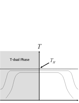
Figure 2: Sketch (based on the analysis of BV of the evolution of temperature $T$ as a function of the radius $R$ of space of a gas of strings in thermal equilibrium. The top curve is characterized by an entropy higher than the bottom curve, and leads to a longer region of Hagedorn behaviour.

If we imagine that there is a dynamical principle that tells us how $R$ evolves in time, then Figure 2 can be interpreted as depicting how the temperature changes as a function of time. If $R$ is a monotonic function of time, then two interesting possibilities for cosmology emerge. If ${\rm ln}R$ decreases to zero at some fixed time (which without loss of generality we can call $t=0$), and continues to decrease, we obtain a temperature profile which is symmetric with respect to $t=0$ and which (since small $R$ is physically equivalent to large $R$) represents a bouncing cosmology (see Biswas2 for a concrete recent realization of this scenario). If, on the other hand, it takes an inifinite amount of time to reach $R=0$, an emergent universe scenario gellis is realized.

It is important to realize that in both of the cosmological scnearios which, as argued above, seem to follow from string theory symmetry considerations alone, a large energy density does not lead to rapid expansion in the Hagedorn phase, in spite of the fact that the matter sources we are considering (namely a gas of strings) obeys all of the usual energy conditions discussed e.g. in HE ). These considerations are telling us that intuition drawn from Einstein gravity may give us a completely incorrect picture of the early universe. This provides a response to the main criticism raised in KKLM .

Any physical theory requires both a specification of the equations of motion and of the initial conditions. We assume that the universe starts out small and hot. For simplicity, we take space to be toroidal, with radii in all spatial directions given by the string scale. We assume that the initial energy density is very high, with an effective temperature which is close to the Hagedorn temperature, the maximal temperature of perturbative string theory.

In this context, it was argued BV that in order for spatial sections to become large, the winding modes need to decay. This decay, at least on a background with stable one cycles such as a torus, is only possible if two winding modes meet and annihilate. Since string world sheets have measure zero probability for intersecting in more than four space-time dimensions, winding modes can annihilate only in three spatial dimensions (see, however, the recent caveats to this conclusion based on the work of Kabat3 ; Danos ). Thus, only three spatial dimensions can become large, hence explaining the observed dimensionality of space-time. As was shown later ABE , adding branes to the system does not change these conclusions since at later times the strings dominate the cosmological dynamics. Note that in the three dimensions which are becoming large there is a natural mechanism of isotropization as long as some winding modes persist Watson1 .

3.3 Equations for String Gas Cosmology

The above arguments were all heuristic. Some of them can be put on a more firm mathematical basis, albeit in the context of a toy model. The toy model consists of a classical background coupled to a gas of strings. From the point of view of rigorous string theory, this separation between classical background and stringy matter is not satisfactory. However, in the absence of a non-perturbative formulation of string theory, at the present time we are forced to make this separation. Note that this separation between classical background geometry and string matter is common to all current approaches to string cosmology.

As our background we choose dilaton gravity. It is crucial to include the dilaton in the Lagrangian, firstly since the dilaton arises in string perturbation theory at the same level as the graviton (when calculating to leading order in the string coupling and in $\alpha^{\prime}$), and secondly because it is only the action of dilaton gravity (rather than the action of Einstein gravity) which is consistent with the T-duality symmetry. We will see, however, that the background dynamics inevitably drives the system into a parameter region where the dilaton is strongly coupled and hence beyond the region of validity of the approximations made.

For the moment, however, we consider the dilaton gravity action coupled to a matter action $S_{m}$

$$S\,=\,{1\over{2\kappa^{2}}}\int d^{10}x\sqrt{-{\hat{g}}}e^{-2\phi}\bigl{[}{\hat{R}}+4\partial^{\mu}\phi\partial_{\mu}\phi\bigr{]}+S_{m}\,,$$ (10)

where ${\hat{g}}$ is the determinant of the metric, ${\hat{R}}$ is the Ricci scalar, $\phi$ is the dilaton, and $\kappa$ is the reduced gravitational constant in ten dimensions. The metric appearing in the above action is the metric in the string frame.

In the case of a homogeneous and isotropic background given by

$$ds^{2}\,=\,dt^{2}-a(t)^{2}d{\bf x}^{2}\,,$$ (11)

the three resulting equations (the generalization of the two Friedmann equations plus the equation for the dilaton) in the string frame are TV (see also Ven )

$$-d{\dot{\lambda}}^{2}+{\dot{\varphi}}^{2}\, = \,e^{\varphi}E$$ (12)

$${\ddot{\lambda}}-{\dot{\varphi}}{\dot{\lambda}}\, = \,{1\over 2}e^{\varphi}P$$ (13)

$${\ddot{\varphi}}-d{\dot{\lambda}}^{2}\, = \,{1\over 2}e^{\varphi}E\,,$$ (14)

where $E$ and $P$ denote the total energy and pressure, respectively, $d$ is the number of spatial dimensions, and we have introduced the logarithm of the scale factor

$$\lambda(t)\,=\,{\rm log}(a(t))$$ (15)

and the rescaled dilaton

$$\varphi\,=\,2\phi-d\lambda\,.$$ (16)

From the second of these equations it follows immediately that a gas of strings containing both stable winding and momentum modes will lead to the stabilization of the radius of the torus: windings prevent expansion, momenta prevent the contraction. The right hand side of the equation can be interpreted as resulting from a confining potential for the scale factor.

Note that this behavior is a consequence of having used dilaton gravity rather than Einstein gravity as the background. The dilaton is evolving at the time when the radius of the torus is at the minimum of its potential. In fact, for the branch of solutions we are considering, the dilaton is increasing as we go into the past. At some point, therefore, it becomes greater than zero. At this point, we enter the region of strong coupling. As already discussed in Riotto , a different dynamical framework is required to analyze this phase. In particular, the fundamental strings are no longer the lightest degrees of freedom. We will call this phase the “strongly coupled Hagedorn phase” for which we lack an analytical description. Since the energy density in this phase is of the string scale, the background equations should also be very different from the dilaton gravity equations used above. In the following section, we will make the assumption that the dilaton is in fact frozen in the strongly coupled Hagedorn phase. This could be a consequence of S-duality (see e.g. Kaya06 for recent studies).

3.4 String Gas Cosmology and Moduli Stabilization

One of the outstanding issues when dealing with theories with extra dimensions is the question of how the size and shape moduli of the extra-dimensional spaces are stabilized. String gas cosmology provides a simple and string-specific mechanism to stabilize most of these moduli (see RHBrev6 for a recent review). The outstanding issue is how to stabilize the dilaton.

It is easiest to first understand radion stabilization in the string frame Watson2 . The mechanism can be immediately seen from the basic equations (12 - 14) of dilaton gravity. From (13) it follows that if the string gas contains both winding and momentum modes, then there is a preferred value for the scale factor. Winding modes prevent the radion from increasing, momentum modes prevent it from decreasing. If the number of winding and momentum modes is the same, then the fixed point of the dynamics corresponds to string-scale radion. As can be seen from (14), the dilaton is evolving when the radion is at the fixed point.

In order to make contact with late-time cosmology, we need to assume that the dilaton is fixed by some non-perturbative mechanism. The issue of radion stabilization is then no longer this simple. A string matter state which minimizes the effective potential in the Einstein frame is only consistent with stabilization if the energy density vanishes at the mininum - otherwise, the state will in fact lead to inflationary expansion. It thus turns out that Subodh1 ; Subodh2 (see also Watson2 ; BattWat2 ) states which are massless and have an enhanced symmetry at a particular radius play a crucial role. If such states exist, then the radion can be fixed at this particular radius (in our case it will be the self-dual radius). Such states exist in the heterotic string theory, but not in Type II string theories where they are projected out by the GSO projection.

To understand stabilization in the Einstein frame, let us consider the equations of motion which arise from coupling the Einstein action (as opposed to the dilaton gravity action) to a string gas. In the anisotropic setting when the metric is taken to be

$$ds^{2}\,=\,dt^{2}-a(t)^{2}d{\bf x}^{2}-\sum_{\alpha=1}^{6}b_{\alpha}(t)^{2}dy_{\alpha}^{2}\,,$$ (17)

where the $y_{\alpha}$ are the internal coordinates, the equations of motion for $b_{\alpha}$ becomes

$${\ddot{b}_{\alpha}}+\bigl{(}3H+\sum_{\beta=1,\beta\neq\alpha}^{6}{{{\dot{b}_{\beta}}}\over{b_{\beta}}}\bigr{)}{\dot{b}_{\alpha}}\,=\,\sum_{n,m}8\pi G{{\mu_{m,n}}\over{\sqrt{g}\epsilon_{m,n}}}{\cal S}\,$$ (18)

where $\mu_{m,n}$ is the number density of $(m,n)$ strings, $\epsilon_{m,n}$ is the energy of an individual $(m,n)$ string, and $g$ is the determinant of the metric. The source term ${\cal S}$ depends on the quantum numbers of the string gas, and the sum runs over all momentum numbers and winding number vectors $m$ and $n$, respectively (note that $n$ and $m$ are six-vectors, one component for each internal dimension). If the number of right-moving oscillator modes is given by $N$, then the source term for fixed $m$ and $n$ is

$${\cal S}\,=\,\sum_{\alpha}\bigl{(}{{m_{\alpha}}\over{b_{\alpha}}}\bigr{)}^{2}-\sum_{\alpha}n_{\alpha}^{2}b_{\alpha}^{2}+{2\over{D-1}}\bigl{[}(n,n)+(n,m)+2(N-1)\bigr{]}\,.$$ (19)

To obtain this equation, we have made use of the mass spectrum of string states and of the level matching conditions. In the case of the bosonic superstring, the mass spectrum for fixed $m,n,N$ and ${\tilde{N}}$, where ${\tilde{N}}$ is the number of left-moving oscillator states, on a six-dimensional torus whose radii are given by $b_{\alpha}$ is

$$m^{2}\,=\,\bigl{(}{{m_{\alpha}}\over{b_{\alpha}}}\bigr{)}^{2}-\sum_{\alpha}n_{\alpha}^{2}b_{\alpha}^{2}+2(N+{\tilde{N}}-2)\,,$$ (20)

and the level matching condition reads

$${\tilde{N}}\,=\,(n,m)+N\,,$$ (21)

where $(n,m)$ indicates the scalar product of $n$ and $m$ in the trivial internal metric.

There are modes which are massless at the self-dual radius $b_{\alpha}=1$. One such mode is the graviton with $n=m=0$ and $N=1$. The modes of interest to us are modes which contain winding and momentum, namely

• $N=1$, $(m,m)=1$, $(m,n)=-1$ and $(n,n)=1$;

• $N=0$, $(m,m)=1$, $(m,n)=1$ and $(n,n)=1$;

• $N=0$ $(m,m)=2$, $(m,n)=0$ and $(n,n)=2$.

Note that some of these modes survive in the Heterotic string theory, but they do not survive the GSO Pol truncation in Type II string theories.

In string theories which admit massless states (i.e. states which are massless at the self-dual radius), these states will dominate the initial partition function. The background dynamics will then also be dominated by these states. To understand the effect of these strings, consider the equation of motion (18) with the source term (19). The first two terms in the source term correspond to an effective potential with a stable minimum at the self-dual radius. However, if the third term in the source does not vanish at the self-dual radius, it will lead to a positive potential which causes the radion to increase. Thus, a condition for the stabilization of $b_{\alpha}$ at the self-dual radius is that the third term in (19) vanish at the self-dual radius. This is the case if and only if the string state is a massless mode.

The massless modes have other nice features which are explored in detail in Subodh2 . They act as radiation from the point of view of our three large dimensions and hence do not lead to an over-abundance problem. As our three spatial dimensions grow, the potential which confines the radion becomes shallower. However, rather surprisingly, it turns out the the potential remains steep enough to avoid fifth force constraints.

Key to the success in simultaneously avoiding the moduli overclosure problem and evading fifth force constraints is the fact that the stabilization mechanism is an intrinsically stringy one, as opposed to an effective field theory mechanism. In the case of effective field theory, both the confining force and the overdensity in the moduli field scale as $V(\varphi)$, where $V(\varphi)$ is the potential energy density of the field $\varphi$. In contrast, in the case of stabilization by means of massless string modes, the energy density in the string modes (from the point of view of our three large dimensions) scales as $p_{3}$, whereas the confining force scales as $p_{3}^{-1}$, where $p_{3}$ is the momentum in the three large dimensions. Thus, for small values of $p_{3}$, one simultaneously gets large confining force (thus satisfying the fifth force constraints) and small energy density Subodh2 .

In the presence of massless string states, the shape moduli also can be stabilized, at least in the simple toroidal backgrounds considered so far Edna (see also Sugumi ). The stabilization mechanism is once again dynamical, and makes use of the massless states with enhanced symmetry (see also Watson3 ; Eva for more on the use of massless states with enhanced symmetries in cosmology).

There has been other recent work on string gas cosmology. The interested reader is referred to other . In particular, the difficulties of dilaton stabilization have been addressed in dilaton . For recent attempts to stabilize the dilaton see Subodh3 and Kaya06 .

4 String Gas Cosmology and Structure Formation

4.1 Overview

Let us recall the key aspects of the dynamics of string gas cosmology. First of all, note that in thermal equilibrium at the string scale ($R\simeq l_{s}$), the self-dual radius, the number of winding and momentum modes will be equal. Since winding and momentum modes give an opposite contribution to the pressure, the pressure of the string gas in thermal equilibrium at the self-dual radius will vanish. From the dilaton gravity equations of motion (12 - 14) it then follows that a static phase $\lambda=0$ will be a fixed point of the dynamical system. This phase is the Hagedorn phase.

On the other hand, for large values of $R$ in thermal equilibrium the energy will be exclusively in momentum modes. These act as usual radiation. Inserting the radiative equation of state into the above equations (12 - 14) it follows that the source in the dilaton equation of motion vanishes and the dilaton approaches a constant as a consequence of the Hubble damping term in its equation of motion. Consequently, the scale factor expands as in the usual radiation-dominated universe.

The transition between the Hagedorn phase and the radiation-dominated phase with fixed dilaton is achieved via the annihilation of winding modes, as studied in detail in BEK . The main point is that, starting in a Hagedorn phase, there will be a smooth transition to the radiation-dominated phase of standard cosmology with fixed dilaton.

Our new cosmological background is obtained by following our currently observed universe into the past according to the string gas cosmology equations. The radiation phase of standard cosmology is unchanged. In particular, the dilaton is fixed in this phase . However, as the temperature of the radiation bath approaches the Hagedorn temperature, the equation of state of string gas matter changes. The equation of state parameter $w=P/E$ decreases towards a pressureless state and the string frame metric becomes static. Note that, in order for the present size of the universe to be larger than our current Hubble radius, the size of the spatial sections in the Hagedorn phase must be at least $1{\rm mm}$ . We will denote the time when the transition from the Hagedorn phase to the radiation phase of standard cosmology occurs by $t_{R}$, to evoque the analogy with the time of reheating in inflationary cosmology. As we go back in time in the Hagedorn phase, the dilaton increases. At the time $t_{c}$ when the dilaton equals zero, a second transition occurs, the transition to a “strongly coupled Hagedorn phase” (using the terminology introduced in Betal ). We take the dilaton to be fixed in this phase. In this case, the strongly coupled Hagedorn phase may have a duration which is very long compared to the Hubble time immediately following $t_{R}$. It is in this cosmological background that we will study the generation of fluctuations.

It is instructive to compare the background evolution of string gas cosmology with the background of inflationary cosmology. Figure 3 is a sketch of the space-time evolution in string gas cosmology. For times $t<t_{R}$, we are in the quasi-static Hagedorn phase, for $t>t_{R}$ we have the radiation-dominated period of standard cosmology. To understand why string gas cosmology can lead to a causal mechanism of structure formation, we must compare the evolution of the physical wavelength corresponding to a fixed comoving scale (fluctuations in early universe cosmology correspond to waves with a fixed wavelength in comoving coordinates) with that of the Hubble radius $H^{-1}(t)$, where $H(t)$ is the expansion rate. The Hubble radius separates scales on which fluctuations oscillate (wavelengths smaller than the Hubble radius) from wavelengths where the fluctuations are frozen in and cannot be effected by microphysics. Causal microphysical processes can generate fluctuations only on sub-Hubble scales (see e.g. RHBrev2 for a concise overview of the theory of cosmological perturbations and MFB for a comprehensive review).

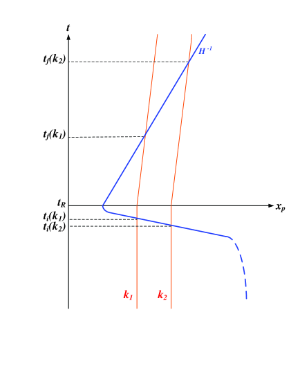
Figure 3: Space-time diagram (sketch) showing the evolution of fixed comoving scales in string gas cosmology. The vertical axis is time, the horizontal axis is physical distance. The Hagedorn phase ends at the time $t_{R}$ and is followed by the radiation-dominated phase of standard cosmology. The solid curve represents the Hubble radius $H^{-1}$ which is cosmological during the quasi-static Hagedorn phase, shrinks abruptly to a microphysical scale at $t_{R}$ and then increases linearly in time for $t>t_{R}$. Fixed comoving scales (the dotted lines labeled by $k_{1}$ and $k_{2}$) which are currently probed in cosmological observations have wavelengths which are smaller than the Hubble radius during the Hagedorn phase. They exit the Hubble radius at times $t_{i}(k)$ just prior to $t_{R}$, and propagate with a wavelength larger than the Hubble radius until they reenter the Hubble radius at times $t_{f}(k)$.

In string gas cosmology, the Hubble radius is infinitely large in the Hagedorn phase. As the universe starts expanding near $t_{R}$, the Hubble radius rapidly decreases to a microscopic value (set by the temperature at $t=t_{R}$ which will be close to the Hagedorn temperature), before turning around and increasing linearly in the post-Hagedorn phase. The physical wavelength corresponding to a fixed comoving scale, on the other hand, is constant during the Hagedorn era. Thus, all scales on which current experiments measure fluctuations are sub-Hubble deep in the Hagedorn phase. In the radiation period, the physical wavelength of a perturbation mode grows only as $\sqrt{t}$. Thus, at a late time $t_{f}(k)$ the fluctuation mode will re-enter the Hubble radius, leading to the perturbations which are observed today.

In contrast, in inflationary cosmology (Figure 1) the Hubble radius is constant during inflation ($t<t_{R}$, where here $t_{R}$ is the time of inflationary reheating), whereas the physical wavelength corresponding to a fixed comoving scale expands exponentially. Thus, as long as the period of inflation is sufficiently long, all scales of interest for current cosmological observations are sub-Hubble at the beginning of inflation.

In spite of the fact that both in inflationary cosmology and in string gas cosmology, scales are sub-Hubble during the early stages, the actual generation mechanism for fluctuations is completely different. In inflationary cosmology, any thermal fluctuations present before the onset of inflation are red-shifted away, leaving us with a quantum vacuum state, whereas in the quasi-static Hagedorn phase of string gas cosmology matter is in a thermal state. Hence, whereas in inflationary cosmology the fluctuations originate as quantum vacuum perturbations, in string gas cosmology the inhomogeneities are created by the thermal fluctuations of the string gas.

As we have shown in NBV ; Ali ; BNPV2 , string thermodynamical fluctuations in the Hagedorn phase of string gas cosmology yield an almost scale-invariant spectrum of both scalar and tensor modes. This result stems from the holographic scaling of the specific heat $C_{V}(R)$ (evaluated for fixed volume) as a function of the radius $R$ of the box

$$C_{V}(R)\,\sim\,R^{2}\,.$$ (22)

As derived in Deo , this result holds true for a gas of closed strings in a space-time in which the three large spatial dimensions are compact. The scaling (22) is an intrinsically stringy result: thermal fluctuations of a gas of particles would lead to a very different scaling.

Since the primordial perturbations in our scenario are of thermal origin (and there are no non-vanishing chemical potentials), they will be adiabatic. The spectrum of scalar metric fluctuations has a slight red tilt. As a distinctive feature BNPV1 , our scenario predicts a slight blue tilt for the spectrum of gravitational waves. The red tilt for the scalar modes is due to the fact that the temperature when short wavelength modes exit the Hubble radius is slightly lower than the temperature when longer wavelength modes exit. The gravitational wave amplitude, in contrast, is determined by the pressure. Since the pressure is closer to zero the deeper in the Hagedorn phase we are, a slight blue tilt for the tensor fluctuations results.

These results are explained in more detail in the following subsections.

4.2 Extracting Metric Fluctuations from Matter Perturbations

In this subsection, we show how the scalar and tensor metric fluctuations can be extracted from knowledge of the energy-momentum tensor of the string gas.

Working in conformal time $\eta$ (defined via $dt=a(t)d\eta$), the metric of a homogeneous and isotropic background space-time perturbed by linear scalar metric fluctuations and gravitational waves can be written in the form

$$ds^{2}=a^{2}(\eta)\left\{(1+2\Phi)d\eta^{2}-[(1-2\Phi)\delta_{ij}+h_{ij}]dx^{i}dx^{j}\right\}\,.$$ (23)

Here, $\Phi$ (which is a function of space and time) describes the scalar metric fluctuations. The tensor $h_{ij}$ is transverse and traceless and contains the two polarization states of the gravitational waves. In the above, we have fixed the coordinate freedom by working in the so-called “longitudinal” gauge in which the scalar metric fluctuation is diagonal. We have also assumed that there is no anisotropic stress. Note that to linear order in the amplitude of the fluctuations, scalar and tensor modes decouple, and the tensor modes are gauge-invariant.

Our approximation scheme for computing the cosmological perturbations and gravitational wave spectra from string gas cosmology is as follows (the analysis is similar to how the calculations were performed in BST ; BK in the case of inflationary cosmology). For a fixed comoving scale $k$ we follow the matter fluctuations until the time $t_{i}(k)$ shortly before the end of the Hagedorn phase when the scale exits the Hubble radius At the time of Hubble radius crossing, we use the Einstein constraint equations (discussed below) to compute the values of $\Phi(k)$ and $h(k)$ ($h$ is the amplitude of the gravitational wave tensor), and then we propagate the metric fluctuations according to the standard gravitational perturbation equations until scales re-enter the Hubble radius at late times. Note that since the dilaton is fixed in the radiation phase, we are justified in using the perturbed Einstein equations after the time $t_{R}$.

Since the dilaton comes to rest at the end of the Hagedorn phase, we will use the Einstein equations to relate the matter fluctuations to the metric perturbations at the time that the scales $k$ exit the Hubble radius at times $t_{i}(k)$. Since $t_{i}(k)<t_{R}$, there are potentially important terms coming from the dilaton velocity which we are neglecting Betal ; KKLM . We will return to this issue later.

Inserting the metric (23) into the Einstein equations, subtracting the background terms and truncating the perturbative expansion at linear order leads to the following system of equations

$$-3{\cal H}\left({\cal H}\Phi+\Phi^{{}^{\prime}}\right)+\nabla^{2}\Phi\, = \,4\pi Ga^{2}\delta T^{0}{}_{0}$$

$$\left({\cal H}\Phi+\Phi^{{}^{\prime}}\right)_{,i}\, = 4\pi Ga^{2}\delta T^{0}{}_{i}$$

$$\left[\left(2{\cal H}^{{}^{\prime}}+{\cal H}^{2}\right)\Phi+3{\cal H}\Phi^{{}^{\prime}}+\Phi^{{}^{\prime\prime}}\right] = -4\pi Ga^{2}\delta T^{i}{}_{i}\,,$$

$$-{1\over 2}\left[{{\cal H}^{\prime}}+{1\over 2}{\cal H}^{2}\right]h_{ij}+{1\over 4}{\cal H}h_{ij}^{\prime}$$

$$+\left[{{\partial^{2}}\over{\partial\eta^{2}}}-\nabla^{2}\right]h_{ij}\, = -4\pi Ga^{2}\delta T^{i}{}_{j}\,,$$ (24)

$$\mbox{for $i\neq j$}\,,$$

where ${\cal H}=a^{\prime}/a$, a prime denotes the derivative with respect to conformal time $\eta$, and $G$ is Newton’s gravitational constant.

In the Hagedorn phase, these equations simplify substantially and allow us to extract the scalar and tensor metric fluctuations individually. Replacing comoving by physical coordinates, we obtain from the $00$ equation

$$\nabla^{2}\Phi\,=\,4\pi G\delta T^{0}{}_{0}\,$$ (25)

and from the $i\neq j$ equation

$$\nabla^{2}h_{ij}\,=\,-4\pi G\delta T^{i}{}_{j}\,.$$ (26)

The above equations (25) and (26) allow us to compute the power spectra of scalar and tensor metric fluctuations in terms of correlation functions of the string energy-momentum tensor. Since the metric perturbations are small in amplitude we can consistently work in Fourier space. Specifically,

$$\langle|\Phi(k)|^{2}\rangle\,=\,16\pi^{2}G^{2}k^{-4}\langle\delta T^{0}{}_{0}(k)\delta T^{0}{}_{0}(k)\rangle\,,$$ (27)

where the pointed brackets indicate expectation values, and

$$\langle|h(k)|^{2}\rangle\,=\,16\pi^{2}G^{2}k^{-4}\langle\delta T^{i}{}_{j}(k)\delta T^{i}{}_{j}(k)\rangle\,,$$ (28)

where on the right hand side of (28) we mean the average over the correlation functions with $i\neq j$.

4.3 String Thermodynamics Fluctuations

Since the Hagedorn phase is quasi-static and dominated by a gas of strings, fluctuations in our scenario are the thermal fluctuations of a gas of strings. We will consider a gas of closed strings in a compact space, i.e. our three-dimensional space is considered to be large but compact. Specifically, it is important to have winding modes in the spectrum of string states.

The correlation functions of the energy-momentum tensor can be obtained from the partition function $Z$, which determines the free energy $F$ via

$$F\,=\,\frac{-1}{\beta}lnZ\,,$$ (29)

where $\beta$ is the inverse temperature.

The expectation value of the energy-momentum tensor $T_{\mu}^{\nu}$ is then given in terms of the free energy by

$$\langle T_{\nu}^{\mu}\rangle\,=\,\frac{-2g_{\nu\lambda}}{\sqrt{-g}}\frac{\delta F}{\delta g_{\lambda\mu}}\,.$$ (30)

Taking one additional variational derivative of (30) we obtain the following expression for the fluctuations of $T_{\mu}^{\nu}$ (see Ali ; BNPV2 for more details):

$$\langle T^{\mu}_{\nu}T^{\kappa}_{\beta}\rangle-\langle T^{\mu}_{\nu}\rangle\langle T^{\kappa}_{\beta}\rangle\,\,=\frac{1}{\beta}\frac{2g_{\beta\tau}}{\sqrt{-g}}\frac{\delta}{\delta g_{\tau\kappa}}\Bigl{(}\frac{-2g_{\nu\lambda}}{\sqrt{-g}}\frac{\delta F}{\delta g_{\lambda\mu}}\Bigr{)}\,.$$ (31)

In particular, the energy density fluctuation is

$$\langle\delta\rho^{2}\rangle\,=\,-\frac{1}{R^{6}}\frac{\partial}{\partial\beta}\left(F+\beta\frac{\partial F}{\partial\beta}\right)\,=\,\frac{T^{2}}{R^{6}}C_{V}\,,$$ (32)

where $C_{V}$ is the specific heat. The off-diagonal pressure fluctuations, in turn, are given by

$$\langle\delta{T^{i}{}_{j}}^{2}\rangle\, = \,\langle{T^{i}{}_{j}}^{2}\rangle-\langle T^{i}{}_{j}\rangle^{2}$$

$$= \,\frac{1}{\beta R^{3}}\frac{\partial}{\partial\ln{R}}\left(-\frac{1}{R^{3}}\frac{\partial F}{\partial\ln{R}}\right)=\frac{1}{\beta R^{2}}\frac{\partial p}{\partial R}\,,$$

where the string pressure is given by

$$p\,\equiv\,-V^{-1}(\partial F/\partial\ln{R})\,=\,T(\partial S/\partial V)_{E}\,.$$ (34)

So far, the analysis has been general thermodynamics. Let us now specialize to the thermodynamics of strings. In Deo , the thermodynamical properties of a gas of closed strings in a toroidal space of radius $R$ were computed. To compute the fluctuations in a region of radius $R$ which forms part of our three-dimensional compact space, we will apply the results of Deo for a box of strings in a volume $V=R^{3}$.

The starting point of the computation is the formula for the density of states $\Omega(E,R)$ which determines the entropy $S$ via

$$S(E,R)\,=\,\ln{\Omega(E,R)}\,.$$ (35)

The entropy, in turn, determines the free energy $F$ from which the correlation functions can be derived. In the Hagedorn phase, the density of states has the following form

$$\Omega(E,R)\,\simeq\,\beta_{H}e^{\beta_{H}E+n_{H}V}[1+\delta\Omega_{(1)}(E,R)]\,,$$ (36)

where $\beta_{H}=T_{H}^{-1}$, $n_{H}$ is a (constant) number density of order $\ell_{s}^{-3}$ ($\ell_{s}$ being the string length), $\rho_{H}$ is the ‘Hagedorn Energy density’ of the order $\ell_{s}^{-4}$, and

$$\ell_{s}^{3}\delta\Omega_{(1)}\,\simeq\,-\frac{R^{2}}{T_{H}}\left(1-\frac{T}{T_{H}}\right)\,.$$ (37)

In addition, we find

$$\langle E\rangle\,\simeq\,\ell_{s}^{-3}R^{2}\ln{\left[\frac{\ell_{s}^{3}T}{R^{2}(1-T/T_{H})}\right]}\,.$$ (38)

Note that to ensure that $|\delta\Omega_{(1)}|\ll 1$ and $\langle E\rangle\gg\rho_{H}R^{3}$, one should demand

$$(1-T/T_{H})R^{2}\ell_{s}^{-2}\ll 1\,.$$ (39)

The results (36) and (37) now allow us to compute the correlation functions (32) and (4.3). We first compute the energy correlation function (32). Making use of (38), it follows from (22) that

$$C_{V}\,\approx\,2\frac{R^{2}/\ell^{3}}{T\left(1-T/T_{H}\right)}\,.$$ (40)

The ‘holographic’ scaling $C_{V}(R)\sim R^{2}$ is responsible for the overall scale-invariance of the spectrum of cosmological perturbations. The factor $(1-T/T_{H})$ in the denominator is responsible for giving the spectrum a slight red tilt. It comes from the differentiation with respect to $T$.

For the pressure. we obtain

$$p(E,R)\approx n_{H}T_{H}-\frac{2}{3}\frac{(1-T/T_{H})}{\ell_{s}^{3}R}\ln{\left[\frac{\ell_{s}^{3}T}{R^{2}(1-T/T_{H})}\right]}\,,$$ (41)

which immediately yields

$$\langle\delta{T^{i}{}_{j}}^{2}\rangle\,\simeq\,\frac{T(1-T/T_{H})}{\ell_{s}^{3}R^{4}}\ln^{2}{\left[\frac{R^{2}}{\ell_{s}^{2}}(1-T/T_{H})\right]}\,.$$ (42)

Note that since no temperature derivative is taken, the factor $(1-T/T_{H})$ remains in the numerator. This leads to the slight blue tilt of the spectrum of gravitational waves. As mentioned earlier, the physical reason for this blue tilt is that larger wavelength modes exit the Hubble radius deeper in the Hagedorn phase where the pressure is smaller and thus the strength of the tensor modes is less.

4.4 Power Spectra

The power spectrum of scalar metric fluctuations is given by

$$P_{\Phi}(k)\, \equiv \,k^{3}|\Phi(k)|^{2}$$

$$= \,16\pi^{2}G^{2}k^{-1}<|\delta\rho(k)|^{2}>\,.$$

$$= \,16\pi^{2}G^{2}k^{2}<(\delta M)^{2}>_{R}$$

$$= \,16\pi^{2}G^{2}k^{-4}<(\delta\rho)^{2}>_{R}\,,$$

where in the first step we have used (27) to replace the expectation value of $|\Phi(k)|^{2}$ in terms of the correlation function of the energy density, and in the second step we have made the transition to position space (note that $k=R^{-1}$).

According to (32), the density correlation function is given by the specific heat via $T^{2}R^{-6}C_{V}$. Inserting the expression from (40) for the specific heat of a string gas on a scale $R$ yields to the final result

$$P_{\Phi}(k)\,=\,16\pi^{2}G^{2}{T\over{\ell_{s}^{3}}}{1\over{1-T/T_{H}}}$$ (44)

for the power spectrum of cosmological fluctuations. In the above equation, the temperature $T$ is to be evaluated at the time $t_{i}(k)$ when the mode $k$ exits the Hubble radius. Since modes with larger values of $k$ exit the Hubble radius slightly later when the temperature is slightly lower, a small red tilt of the spectrum is induced. The amplitude ${\cal A}_{S}$ of the power spectrum is given by

$${\cal A}_{S}\,\sim\,\bigl{(}{{l_{pl}}\over{l_{s}}}\bigr{)}^{4}{1\over{1-T/T_{H}}}\,.$$ (45)

Taking the last factor to be of order unity, we find that a string length three orders of magnitude larger than the Planck length, a string length which was assumed in early studies of string theory, gives the correct amplitude of the spectrum. Thus, it appears that the string gas cosmology structure formation mechanism does not have a serious amplitude problem.

Similarly, we can compute the power spectrum of the gravitational waves and obtain

$$P_{h}(k)\,\sim\,16\pi^{2}G^{2}{T\over{\ell_{s}^{3}}}(1-T/T_{H})\ln^{2}{\left[\frac{1}{\ell_{s}^{2}k^{2}}(1-T/T_{H})^{-1}\right]}\,.$$ (46)

This shows that the spectrum of tensor modes is - to a first approximation, namely neglecting the logarithmic factor and neglecting the k-dependence of $T(t_{i}(k))$ - scale-invariant . The k-dependence of the temperature at Hubble radius crossing induces a small blue tilt for the spectrum of gravitational waves.

Comparing (44) and (46) we see that the tensor to scalar ratio is suppressed by the factor $(1-T/T_{H})^{2}$. Given a good understanding of the exit from the Hagedorn phase we would be able to compute this ratio as well as the magnitude of the spectral tilts for both scalar and tensor modes.

4.5 The Strongly Coupled Hagedorn Phase

In the previous discussion we have assumed that during the Hagedorn phase, the kinetic energy of the dilaton has negligible effects. However, this is not the case Betal ; KKLM if the background is described in terms of dilaton gravity. However, as stressed in Section 2.6, it is unrealisitc to expect that pure dilaton gravity is a good approximation to the dyanamics of the Hagedorn phase. Both string loop and $\alpha^{\prime}$ corrections will be important. Another aspect of this issue is that - according to the dilaton gravity equations - the string coupling constant quickly becomes greater than unity as we go back in time from $t_{R}$. At that point, the separation between classical dilaton background and stringy matter becomes untenable.

Therefore, in order to put our scenario on a firm basis, we need a consistent description of the Hagedorn phase. It is crucial that there be a phase before or immediately leading up to $t_{R}$, the time when the winding string modes decay to string loops, when the dilaton is fixed. In this case, the calculations we have done above are well justified.

Let us assume, for example, that the dilaton gets fixed once it reaches its self-dual value, at a time which we denote by $t_{c}$. Freezing the dilaton allows the Hagedorn phase to be of sufficiently long duration for thermal string equilibrium to be established on scales up to $1{\rm mm}$. It will also put out structure formation scenario on a more solid footing. In this case, the space-time diagram is given by Fig. 4, where we are now plotting scales consistently in the Einstein frame. As is apparent, the overall structure of the diagram is the same as that of Fig. 3, except for the fact that scales exit the Einstein frame Hubble radius at a time $t_{i}(k)$ immediately before $t_{c}$ instead of immediately before $t_{R}$. A valid concern is that we might not be allowed to neglect the higher derivative terms in the gravitational action at such early times during the Hagedorn phase.

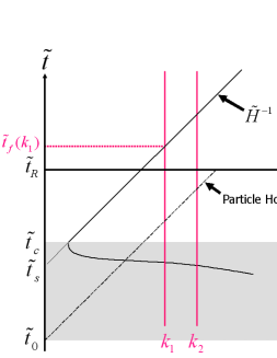
Figure 4: Space-time diagram (sketch) showing the evolution of fixed comoving scales in string gas cosmology. The vertical axis is Einstein frame time, the horizontal axis is comoving distance. The solid curve represents the Einstein frame Hubble radius ${\tilde{H}}^{-1}$ which is linearly increasing after ${\tilde{t}}_{c}$. Fixed comoving scales (the dotted lines labeled by $k_{1}$ and $k_{2}$) which are currently probed in cosmological observations have wavelengths which are larger than the Einstein frame Hubble radius during the part of the Hagedorn phase in which the dilaton is rolling. However, due to the presence of the initial strong coupling Hagedorn phase, the horizon becomes much larger than the Hubble radius. The shaded region corresponds to the strong coupling Hagedorn phase.

A background in which our string gas structure formation scenario can be implemented Biswas2 is the ghost-free and asymptotically free higher derivative gravity model proposed in Biswas given by the gravitational action

$$S\,=\,\int d^{4}x\sqrt{-g}F(R)$$ (47)

with

$$F(R)\,=\,R+\sum_{n=0}^{\infty}{{c_{n}}\over{M_{s}^{2n}}}R\bigl{(}{{\partial^{2}}\over{\partial^{2}t}}-\nabla^{2}\bigr{)}^{n}R\,,$$ (48)

where $M_{s}$ is the string mass scale (more generally, it is the scale where non-perturbative effects start to dominate), and the $c_{n}$ are coefficients of order unity.

As shown in Biswas and Biswas2 , this action has bouncing cosmological solutions. If the temperature during the bounce phase is sufficiently high, then a gas of strings will be excited in this phase. In the absence of initial cosmological perturbations in the contracting phase, our string gas structure formation scenario is realized. The string network will contain winding modes in the same way that a string network formed during a cosmological phase transition will contain infinite strings. The dilaton is fixed in this scenario, thus putting the calculation of the cosmological perturbations on a firm basis. There are no additional dynamical degrees of freedom compared to those in Einstein gravity. The higher derivative corrections to the equations of motion (in particular to the Poisson equation) are suppressed by factors of $(k/M_{s})^{2}$. Thus, all of the conditions on a cosmological backgroound to successfully realize the string gas cosmology structure formation scenario are realized.

5 Discussion

In spite of the great phenomenological successes at solving key problems of Standard Big Bang cosmology such as the horizon, entropy and flatness problems, and at providing a simple and predictive structure formation scenario, current realizations of inflation are beset by important conceptual problems. Most importantly, the applicability of effective field theory techniques and Einstein gravity intuition at energy scales close to the string and Planck scales are questionable.

New input from fundamental physics is required to address the problems of our current models of inflation. It is likely that superstring theory will lead to a new paradigm of early universe cosmology. Such a new paradigm may yield a convincing realization of inflation, but it may also give rise to a quite different scenario for early universe cosmology.

We have presented a new cosmological background motivated by key symmetries and making use of new degrees of freedom of string theory. This background is characterized by an early quasi-static Hagedorn phase during which the matter content of the universe is a thermal gas of strings. The decay of string winding modes leads to a smooth transition to the radiation phase of standard cosmology, without an intervening period of inflation. However, thermal fluctuations of strings during the Hagedorn phase yields a new structure formation scenario. The holographic scaling of the specific heat of a gas of closed strings on a compact three-dimensional space then leads to an almost scale-invariant spectrum of cosmological perturbations. A key prediction of this scneario is a slight blue tilt of the spectrum of gravitational waves. Note that the spectrum of the scalar modes has a slight red tilt.

There are many outstanding issues. We have presented a potential alternative solution for the origin of structure in the universe. Inflation, however, has other key successes. Most importantly, it generates a large, homogeneous, high entropy and spatially flat universe starting from initial conditions where space is small and has only a low entropy. Are there alternatives to solving these problems which arise from string gas cosmology? If the universe starts out cold and large (natural initial conditions in the context of a bouncing universe scenario), the above problems do not arise. Since string gas cosmology may well lead to a bouncing cosmology, as in the setup of Biswas , this possibility should be kept in mind. Alternatively, starting from initial conditions where all dimensions of space start out small, there may be an initial phase of bulk dynamics which telescopes an initial string scale into the required scale of $1{\rm mm}$ during the Hagedorn phase (see Natalia for an example).

Another outstanding issue is to obtain a better understanding of the dynamics of the Hagedorn phase. Dilaton gravity does not provide the adequate background equations, in particular at early stages during the Hagedorn phase. An improved understanding of the background dynamics is also required in order to be able to calculate the temperature $T(t_{i}(k))$ at the time when scales $k$ exit the Hubble radius. The value of the temperature and its k-dependence are crucial in order to be able to calculate the magnitude of the tilt of the power spectra of fluctuations as well as the tensor to scalar ratio.

Acknowledgements

I would like to thank the organizers of the Colloque 2006 of the IAP for inviting me to speak and for their generous hospitality during this stimulating conference. I wish to thank my collaborators Ali Nayeri, Subodh Patil and Cumrun Vafa for a most enjoyable collaboration. I also thank Lev Kofman, Andrei Linde and Slava Mukhanov for vigorous discussions which helped clarify some of the points presented in Subsection 4.5. Some of the arguments in that subsection were finalized after the Colloque, and appeared in Betal . I am grateful to Sugumi Kanno, Jiro Soda, Damien Easson, Justin Khoury, Patrick Martineau, Ali Nayeri and Subodh Patil for their collaboration on this paper, and I in particular thank Sugumi Kanno for allowing me to use three figures of Betal in this writeup. I also with to thank Tirthabir Biswas for extensive discussions. My research is supported by an NSERC Discovery Grant and by the Canada Research Chairs program.

References

- (1) A. H. Guth, “The Inflationary Universe: A Possible Solution To The Horizon And Flatness Problems,” Phys. Rev. D 23, 347 (1981).
- (2) K. Sato, “First Order Phase Transition Of A Vacuum And Expansion Of The Universe,” Mon. Not. Roy. Astron. Soc. 195, 467 (1981).
- (3) A. A. Starobinsky, “A New Type Of Isotropic Cosmological Models Without Singularity,” Phys. Lett. B 91, 99 (1980).
- (4) R. Brout, F. Englert and E. Gunzig, “The Creation Of The Universe As A Quantum Phenomenon,” Annals Phys. 115, 78 (1978).
- (5) V. F. Mukhanov and G. V. Chibisov, “Quantum Fluctuation And ’Nonsingular’ Universe. (In Russian),” JETP Lett. 33, 532 (1981) [Pisma Zh. Eksp. Teor. Fiz. 33, 549 (1981)].
- (6) W. Press, Phys. Scr. 21, 702 (1980).
- (7) A. A. Starobinsky, “Spectrum Of Relict Gravitational Radiation And The Early State Of The Universe,” JETP Lett. 30, 682 (1979) [Pisma Zh. Eksp. Teor. Fiz. 30, 719 (1979)].
- (8) R. A. Sunyaev and Y. B. Zeldovich, “Small scale fluctuations of relic radiation,” Astrophys. Space Sci. 7, 3 (1970).
- (9) P. J. E. Peebles and J. T. Yu, “Primeval adiabatic perturbation in an expanding universe,” Astrophys. J. 162, 815 (1970).
- (10) G. F. Smoot et al., “Structure in the COBE DMR first year maps,” Astrophys. J. 396, L1 (1992).
- (11) P. de Bernardis et al. [Boomerang Collaboration], “A Flat Universe from High-Resolution Maps of the Cosmic Microwave Background Radiation,” Nature 404, 955 (2000) [arXiv:astro-ph/0004404].
- (12) C. L. Bennett et al., “First Year Wilkinson Microwave Anisotropy Probe (WMAP) Observations: Preliminary Maps and Basic Results,” Astrophys. J. Suppl. 148, 1 (2003) [arXiv:astro-ph/0302207].
- (13) C. P. Burgess, “Inflatable string theory?,” Pramana 63, 1269 (2004) [arXiv:hep-th/0408037].
- (14) J. M. Cline, “Inflation from string theory,” arXiv:hep-th/0501179.
- (15) A. Linde, “Inflation and string cosmology,” eConf C040802, L024 (2004) [arXiv:hep-th/0503195].
- (16) A. Nayeri, R. H. Brandenberger and C. Vafa, “Producing a scale-invariant spectrum of perturbations in a Hagedorn phase of string cosmology,” Phys. Rev. Lett. 97, 021302 (2006) [arXiv:hep-th/0511140].
- (17) A. Nayeri, “Inflation free, stringy generation of scale-invariant cosmological fluctuations in D = 3 + 1 dimensions,” arXiv:hep-th/0607073.
- (18) R. H. Brandenberger, A. Nayeri, S. P. Patil and C. Vafa, “String gas cosmology and structure formation,” arXiv:hep-th/0608121.
- (19) R. H. Brandenberger, A. Nayeri, S. P. Patil and C. Vafa, “Tensor modes from a primordial Hagedorn phase of string cosmology,” arXiv:hep-th/0604126.
- (20) R. H. Brandenberger et al., “More on the spectrum of perturbations in string gas cosmology,” JCAP 0611, 009 (2006) [arXiv:hep-th/0608186].
- (21) M. Sasaki, “Large Scale Quantum Fluctuations In The Inflationary Universe,” Prog. Theor. Phys. 76, 1036 (1986).
- (22) V. F. Mukhanov, “Quantum Theory Of Gauge Invariant Cosmological Perturbations,” Sov. Phys. JETP 67, 1297 (1988) [Zh. Eksp. Teor. Fiz. 94N7, 1 (1988)].
- (23) V. F. Mukhanov, H. A. Feldman and R. H. Brandenberger, “Theory of cosmological perturbations. Part 1. Classical perturbations. Part 2. Quantum theory of perturbations. Part 3. Extensions,” Phys. Rept. 215, 203 (1992).
- (24) R. H. Brandenberger, “Lectures on the theory of cosmological perturbations,” Lect. Notes Phys. 646, 127 (2004) [arXiv:hep-th/0306071].
- (25) V. Mukhanov, “CMB-slow, or How to Estimate Cosmological Parameters by Hand,” arXiv:astro-ph/0303072.
- (26) A. D. Linde, “Chaotic Inflation,” Phys. Lett. B 129, 177 (1983).
- (27) A. D. Linde, “Hybrid inflation,” Phys. Rev. D 49, 748 (1994) [arXiv:astro-ph/9307002].
- (28) R. H. Brandenberger and J. H. Kung, “Chaotic Inflation As An Attractor In Initial Condition Space,” Phys. Rev. D 42, 1008 (1990).
- (29) H. A. Feldman and R. H. Brandenberger, “Chaotic Inflation With Metric And Matter Perturbations,” Phys. Lett. B 227, 359 (1989).
- (30) D. S. Goldwirth and T. Piran, “Initial conditions for inflation,” Phys. Rept. 214, 223 (1992).
-
(31)
A. D. Linde,
“A New Inflationary Universe Scenario: A Possible Solution Of The Horizon,
Flatness, Homogeneity, Isotropy And Primordial Monopole Problems,”
Phys. Lett. B 108, 389 (1982);
A. Albrecht and P. J. Steinhardt, “Cosmology For Grand Unified Theories With Radiatively Induced Symmetry Breaking,” Phys. Rev. Lett. 48, 1220 (1982). - (32) R. Brandenberger, G. Geshnizjani and S. Watson, “On the initial conditions for brane inflation,” Phys. Rev. D 67, 123510 (2003) [arXiv:hep-th/0302222].
-
(33)
A. D. Linde,
“Eternal Chaotic Inflation,”
Mod. Phys. Lett. A 1, 81 (1986);
A. D. Linde and D. A. Linde, “Topological defects as seeds for eternal inflation,” Phys. Rev. D 50, 2456 (1994) [arXiv:hep-th/9402115]. - (34) R. Allahverdi, K. Enqvist, J. Garcia-Bellido and A. Mazumdar, “Gauge invariant MSSM inflaton,” arXiv:hep-ph/0605035.
- (35) F. C. Adams, K. Freese and A. H. Guth, “Constraints On The Scalar Field Potential In Inflationary Models,” Phys. Rev. D 43, 965 (1991).
- (36) A. Vilenkin and E.P.S. Shellard, Cosmic Strings and other Topological Defects (Cambridge Univ. Press, Cambridge, 1994).
- (37) M. B. Hindmarsh and T. W. B. Kibble, “Cosmic strings,” Rept. Prog. Phys. 58, 477 (1995) [arXiv:hep-ph/9411342].
- (38) R. H. Brandenberger, “Topological defects and structure formation,” Int. J. Mod. Phys. A 9, 2117 (1994) [arXiv:astro-ph/9310041].
-
(39)
N. Turok and R. H. Brandenberger,
“Cosmic Strings And The Formation Of Galaxies And Clusters Of Galaxies,”
Phys. Rev. D 33, 2175 (1986);
H. Sato, “Galaxy Formation by Cosmic Strings,” Prog. Theor. Phys. 75, 1342 (1986);
A. Stebbins, “Cosmic Strings and Cold Matter”, Ap. J. (Lett.) 303, L21 (1986). -
(40)
A. Albrecht, D. Coulson, P. Ferreira and J. Magueijo,
“Causality and the microwave background,”
Phys. Rev. Lett. 76, 1413 (1996)
[arXiv:astro-ph/9505030];
J. Magueijo, A. Albrecht, D. Coulson and P. Ferreira, “Doppler peaks from active perturbations,” Phys. Rev. Lett. 76, 2617 (1996) [arXiv:astro-ph/9511042];
U. L. Pen, U. Seljak and N. Turok, “Power spectra in global defect theories of cosmic structure formation,” Phys. Rev. Lett. 79, 1611 (1997) [arXiv:astro-ph/9704165]. - (41) R. H. Brandenberger, “Inflationary cosmology: Progress and problems,” publ. in proc. of IPM School On Cosmology 1999: Large Scale Structure Formation, arXiv:hep-ph/9910410.
-
(42)
R. H. Brandenberger and J. Martin, “The robustness of inflation to changes in super-Planck-scale physics,”
Mod. Phys. Lett. A 16, 999 (2001),
[arXiv:astro-ph/0005432];
J. Martin and R. H. Brandenberger, “The trans-Planckian problem of inflationary cosmology,” Phys. Rev. D 63, 123501 (2001), [arXiv:hep-th/0005209]. -
(43)
J. C. Niemeyer,
“Inflation with a high frequency cutoff,”
Phys. Rev. D 63, 123502 (2001),
[arXiv:astro-ph/0005533];
S. Shankaranarayanan, “Is there an imprint of Planck scale physics on inflationary cosmology?,” Class. Quant. Grav. 20, 75 (2003), [arXiv:gr-qc/0203060];
J. C. Niemeyer and R. Parentani, “Trans-Planckian dispersion and scale-invariance of inflationary perturbations,” Phys. Rev. D 64, 101301 (2001), [arXiv:astro-ph/0101451]. - (44) W. G. Unruh, “Sonic analog of black holes and the effects of high frequencies on black hole evaporation,” Phys. Rev. D 51, 2827 (1995).
- (45) S. Corley and T. Jacobson, “Hawking Spectrum and High Frequency Dispersion,” Phys. Rev. D 54, 1568 (1996) [arXiv:hep-th/9601073].
- (46) R. H. Brandenberger and J. Martin, “Back-reaction and the trans-Planckian problem of inflation revisited,” Phys. Rev. D 71, 023504 (2005) [arXiv:hep-th/0410223].
- (47) T. Tanaka, “A comment on trans-Planckian physics in inflationary universe,” [arXiv:astro-ph/0012431].
- (48) A. A. Starobinsky, “Robustness of the inflationary perturbation spectrum to trans-Planckian physics,” Pisma Zh. Eksp. Teor. Fiz. 73, 415 (2001), [JETP Lett. 73, 371 (2001)], [arXiv:astro-ph/0104043].
-
(49)
C. S. Chu, B. R. Greene and G. Shiu,
“Remarks on inflation and noncommutative geometry,”
Mod. Phys. Lett. A 16, 2231
(2001), [arXiv:hep-th/0011241];
R. Easther, B. R. Greene, W. H. Kinney and G. Shiu, “Inflation as a probe of short distance physics,” Phys. Rev. D 64, 103502 (2001), [arXiv:hep-th/0104102];
R. Easther, B. R. Greene, W. H. Kinney and G. Shiu, “Imprints of short distance physics on inflationary cosmology,” Phys. Rev. D 67, 063508 (2003), [arXiv:hep-th/0110226];
F. Lizzi, G. Mangano, G. Miele and M. Peloso, “Cosmological perturbations and short distance physics from noncommutative geometry,” JHEP 0206, 049 (2002) [arXiv:hep-th/0203099];
S. F. Hassan and M. S. Sloth, “Trans-Planckian effects in inflationary cosmology and the modified uncertainty principle,” Nucl. Phys. B 674, 434 (2003), [arXiv:hep-th/0204110]. - (50) R. Brandenberger and P. M. Ho, “Noncommutative spacetime, stringy spacetime uncertainty principle, and density fluctuations,” Phys. Rev. D 66, 023517 (2002), [AAPPS Bull. 12N1, 10 (2002)], [arXiv:hep-th/0203119].
- (51) A. Kempf and J. C. Niemeyer, “Perturbation spectrum in inflation with cutoff,” Phys. Rev. D 64, 103501 (2001), [arXiv:astro-ph/0103225].
-
(52)
U. H. Danielsson, Phys. Rev. D 66, 023511 (2002),
“A note on inflation and transplanckian physics,”
[arXiv:hep-th/0203198];
V. Bozza, M. Giovannini and G. Veneziano, JCAP 0305, 001 (2003), “Cosmological perturbations from a new-physics hypersurface,” [arXiv:hep-th/0302184];
J. C. Niemeyer, R. Parentani and D. Campo, “Minimal modifications of the primordial power spectrum from an adiabatic short distance cutoff,” Phys. Rev. D 66, 083510 (2002) [arXiv:hep-th/0206149]. -
(53)
C. P. Burgess, J. M. Cline, F. Lemieux and R. Holman,
“Are inflationary predictions sensitive to very high energy physics?,”
JHEP 0302, 048 (2003)
[arXiv:hep-th/0210233];
K. Schalm, G. Shiu and J. P. van der Schaar, “The cosmological vacuum ambiguity, effective actions, and transplanckian effects in inflation,” AIP Conf. Proc. 743, 362 (2005) [arXiv:hep-th/0412288]. - (54) J. Martin and R. Brandenberger, “On the dependence of the spectra of fluctuations in inflationary cosmology on trans-Planckian physics,” Phys. Rev. D 68, 063513 (2003) [arXiv:hep-th/0305161].
- (55) S. Hawking and G. Ellis, The Large-Scale Structure of Space-Time (Cambridge Univ. Press, Cambridge, 1973).
- (56) A. Borde and A. Vilenkin, “Eternal inflation and the initial singularity,” Phys. Rev. Lett. 72, 3305 (1994) [arXiv:gr-qc/9312022].
- (57) N. Arkani-Hamed, L. Motl, A. Nicolis and C. Vafa, “The string landscape, black holes and gravity as the weakest force,” arXiv:hep-th/0601001.
-
(58)
R. H. Brandenberger, V. F. Mukhanov and A. Sornborger,
“A Cosmological theory without singularities,”
Phys. Rev. D 48, 1629 (1993)
[arXiv:gr-qc/9303001];
V. F. Mukhanov and R. H. Brandenberger, “A Nonsingular universe,” Phys. Rev. Lett. 68, 1969 (1992). - (59) T. Biswas, A. Mazumdar and W. Siegel, “Bouncing universes in string-inspired gravity,” JCAP 0603, 009 (2006) [arXiv:hep-th/0508194].
- (60) M. Bojowald, “Loop quantum cosmology,” Living Rev. Rel. 8, 11 (2005) [arXiv:gr-qc/0601085].
- (61) R. Hagedorn, “Statistical Thermodynamics Of Strong Interactions At High-Energies,” Nuovo Cim. Suppl. 3, 147 (1965).
- (62) R. H. Brandenberger and C. Vafa, “Superstrings In The Early Universe,” Nucl. Phys. B 316, 391 (1989).
- (63) R. H. Brandenberger, “Back reaction of cosmological perturbations and the cosmological constant problem,” publ. in the proc. of the 18th IAP Colloquium On The Nature Of Dark Energy: Observational And Theoretical Results On The Accelerating Universe, arXiv:hep-th/0210165.
- (64) P. Brax, C. van de Bruck and A. C. Davis, “Brane world cosmology,” Rept. Prog. Phys. 67, 2183 (2004) [arXiv:hep-th/0404011].
- (65) M. Majumdar and A.-C. Davis, “Cosmological creation of D-branes and anti-D-branes,” JHEP 0203, 056 (2002) [arXiv:hep-th/0202148].
- (66) R. Durrer, M. Kunz and M. Sakellariadou, “Why do we live in 3+1 dimensions?,” Phys. Lett. B 614, 125 (2005) [arXiv:hep-th/0501163].
- (67) A. Karch and L. Randall, “Relaxing to three dimensions,” Phys. Rev. Lett. 95, 161601 (2005) [arXiv:hep-th/0506053].
- (68) A. A. Tseytlin and C. Vafa, “Elements of string cosmology,” Nucl. Phys. B 372, 443 (1992) [arXiv:hep-th/9109048].
- (69) S. Alexander, R. H. Brandenberger and D. Easson, “Brane gases in the early universe,” Phys. Rev. D 62, 103509 (2000) [arXiv:hep-th/0005212].
- (70) J. Kripfganz and H. Perlt, “Cosmological Impact Of Winding Strings,” Class. Quant. Grav. 5, 453 (1988).
- (71) T. Battefeld and S. Watson, “String gas cosmology,” Rev. Mod. Phys. 78, 435 (2006) [arXiv:hep-th/0510022].
- (72) R. H. Brandenberger, “Challenges for string gas cosmology,” publ. in proc. of the 59th Yamada Conference On Inflating Horizon Of Particle Astrophysics And Cosmology, arXiv:hep-th/0509099.
- (73) R. H. Brandenberger, “Moduli stabilization in string gas cosmology,” Prog. Theor. Phys. Suppl. 163, 358 (2006) [arXiv:hep-th/0509159].
- (74) J. Polchinski, String Theory, Vols. 1 and 2, (Cambridge Univ. Press, Cambridge, 1998).
- (75) T. Boehm and R. Brandenberger, “On T-duality in brane gas cosmology,” JCAP 0306, 008 (2003) [arXiv:hep-th/0208188].
- (76) T. Biswas, R. Brandenberger, A. Mazumdar and W. Siegel, “Non-perturbative gravity, Hagedorn bounce and CMB,” arXiv:hep-th/0610274.
- (77) G. F. R. Ellis and R. Maartens, “The emergent universe: Inflationary cosmology with no singularity,” Class. Quant. Grav. 21, 223 (2004) [arXiv:gr-qc/0211082].
- (78) N. Kaloper, L. Kofman, A. Linde and V. Mukhanov, “On the new string theory inspired mechanism of generation of cosmological perturbations,” JCAP 0610, 006 (2006) [arXiv:hep-th/0608200].
- (79) R. Easther, B. R. Greene, M. G. Jackson and D. Kabat, “String windings in the early universe,” JCAP 0502, 009 (2005) [arXiv:hep-th/0409121].
- (80) R. Danos, A. R. Frey and A. Mazumdar, “Interaction rates in string gas cosmology,” Phys. Rev. D 70, 106010 (2004) [arXiv:hep-th/0409162].
- (81) S. Watson and R. H. Brandenberger, “Isotropization in brane gas cosmology,” Phys. Rev. D 67, 043510 (2003) [arXiv:hep-th/0207168].
- (82) G. Veneziano, “Scale factor duality for classical and quantum strings,” Phys. Lett. B 265, 287 (1991).
- (83) M. Maggiore and A. Riotto, “D-branes and cosmology,” Nucl. Phys. B 548, 427 (1999) [arXiv:hep-th/9811089].
-
(84)
S. P. Patil,
“Moduli (dilaton, volume and shape) stabilization via massless F and D
arXiv:hep-th/0504145;
S. Cremonini and S. Watson, “Dilaton dynamics from production of tensionless membranes,” Phys. Rev. D 73, 086007 (2006) [arXiv:hep-th/0601082];
S. Arapoglu, A. Karakci and A. Kaya, “S-duality in string gas cosmology,” arXiv:hep-th/0611193. - (85) S. Watson and R. Brandenberger, “Stabilization of extra dimensions at tree level,” JCAP 0311, 008 (2003) [arXiv:hep-th/0307044].
- (86) S. P. Patil and R. Brandenberger, “Radion stabilization by stringy effects in general relativity and dilaton gravity,” Phys. Rev. D 71, 103522 (2005) [arXiv:hep-th/0401037].
- (87) S. P. Patil and R. H. Brandenberger, “The cosmology of massless string modes,” JCAP 0601, 005 (2006) [arXiv:hep-th/0502069].
- (88) T. Battefeld and S. Watson, “Effective field theory approach to string gas cosmology,” JCAP 0406, 001 (2004) [arXiv:hep-th/0403075].
- (89) R. Brandenberger, Y. K. Cheung and S. Watson, “Moduli stabilization with string gases and fluxes,” JHEP 0605, 025 (2006) [arXiv:hep-th/0501032].
- (90) S. Kanno and J. Soda, “Moduli Stabilization in String Gas Cosmology,” Phys. Rev. D 72, 104023 (2005) [arXiv:hep-th/0509074].
- (91) S. Watson, “Moduli stabilization with the string Higgs effect,” Phys. Rev. D 70, 066005 (2004) [arXiv:hep-th/0404177].
- (92) L. Kofman, A. Linde, X. Liu, A. Maloney, L. McAllister and E. Silverstein, “Beauty is attractive: Moduli trapping at enhanced symmetry points,” JHEP 0405, 030 (2004) [arXiv:hep-th/0403001].
-
(93)
G. B. Cleaver and P. J. Rosenthal,
“String cosmology and the dimension of space-time,”
Nucl. Phys. B 457, 621 (1995)
[arXiv:hep-th/9402088];
M. Sakellariadou, “Numerical Experiments in String Cosmology,” Nucl. Phys. B 468, 319 (1996) [arXiv:hep-th/9511075];
R. Easther, B. R. Greene and M. G. Jackson, “Cosmological string gas on orbifolds,” Phys. Rev. D 66, 023502 (2002) [arXiv:hep-th/0204099]l
R. Easther, B. R. Greene, M. G. Jackson and D. Kabat, “Brane gas cosmology in M-theory: Late time behavior,” Phys. Rev. D 67, 123501 (2003) [arXiv:hep-th/0211124];
R. Easther, B. R. Greene, M. G. Jackson and D. Kabat, “Brane gases in the early universe: Thermodynamics and cosmology,” JCAP 0401, 006 (2004) [arXiv:hep-th/0307233];
S. H. S. Alexander, “Brane gas cosmology, M-theory and little string theory,” JHEP 0310, 013 (2003) [arXiv:hep-th/0212151];
B. A. Bassett, M. Borunda, M. Serone and S. Tsujikawa, “Aspects of string-gas cosmology at finite temperature,” Phys. Rev. D 67, 123506 (2003) [arXiv:hep-th/0301180];
D. A. Easson, “Brane gases on K3 and Calabi-Yau manifolds,” Int. J. Mod. Phys. A 18, 4295 (2003) [arXiv:hep-th/0110225];
A. Campos, “Late-time dynamics of brane gas cosmology,” Phys. Rev. D 68, 104017 (2003) [arXiv:hep-th/0304216];
T. Biswas, “Cosmology with branes wrapping curved internal manifolds,” JHEP 0402, 039 (2004) [arXiv:hep-th/0311076];
A. Kaya and T. Rador, “Wrapped branes and compact extra dimensions in cosmology,” Phys. Lett. B 565, 19 (2003) [arXiv:hep-th/0301031];
A. Kaya, “On winding branes and cosmological evolution of extra dimensions in string theory,” Class. Quant. Grav. 20, 4533 (2003) [arXiv:hep-th/0302118];
A. Campos, “Late cosmology of brane gases with a two-form field,” Phys. Lett. B 586, 133 (2004) [arXiv:hep-th/0311144];
S. Watson and R. Brandenberger, “Linear perturbations in brane gas cosmology,” JHEP 0403, 045 (2004) [arXiv:hep-th/0312097];
S. Watson, “UV perturbations in brane gas cosmology,” Phys. Rev. D 70, 023516 (2004) [arXiv:hep-th/0402015];
R. Brandenberger, D. A. Easson and A. Mazumdar, “Inflation and brane gases,” Phys. Rev. D 71, 083514 (2005) [arXiv:hep-th/0307043];
A. Kaya, “Volume stabilization and acceleration in brane gas cosmology,” JCAP 0408, 014 (2004) [arXiv:hep-th/0405099];
S. Arapoglu and A. Kaya, “D-brane gases and stabilization of extra dimensions in dilaton gravity,” Phys. Lett. B 603, 107 (2004) [arXiv:hep-th/0409094];
T. Rador, “Intersection democracy for winding branes and stabilization of extra dimensions,” Phys. Lett. B 621, 176 (2005) [arXiv:hep-th/0501249];
T. Rador, “Vibrating winding branes, wrapping democracy and stabilization of extra dimensions in dilaton gravity,” JHEP 0506, 001 (2005) [arXiv:hep-th/0502039];
T. Rador, “Stabilization of extra dimensions and the dimensionality of the observed space,” arXiv:hep-th/0504047;
A. Kaya, “Brane gases and stabilization of shape moduli with momentum and winding stress,” Phys. Rev. D 72, 066006 (2005) [arXiv:hep-th/0504208];
F. Ferrer and S. Rasanen, “Dark energy and decompactification in string gas cosmology,” JHEP 0602, 016 (2006) [arXiv:hep-th/0509225];
M. Borunda and L. Boubekeur, “The effect of alpha’ corrections in string gas cosmology,” JCAP 0610, 002 (2006) [arXiv:hep-th/0604085];
A. Chatrabhuti, “Target space duality and moduli stabilization in string gas cosmology,” arXiv:hep-th/0602031;
J. Y. Kim, “Stabilization of the extra dimensions in brane gas cosmology with bulk flux,” arXiv:hep-th/0608131. -
(94)
A. J. Berndsen and J. M. Cline,
“Dilaton stabilization in brane gas cosmology,”
Int. J. Mod. Phys. A 19, 5311 (2004)
[arXiv:hep-th/0408185];
A. Berndsen, T. Biswas and J. M. Cline, “Moduli stabilization in brane gas cosmology with superpotentials,” JCAP 0508, 012 (2005) [arXiv:hep-th/0505151];
D. A. Easson and M. Trodden, “Moduli stabilization and inflation using wrapped branes,” Phys. Rev. D 72, 026002 (2005) [arXiv:hep-th/0505098];
S. Cremonini and S. Watson, “Dilaton dynamics from production of tensionless membranes,” Phys. Rev. D 73, 086007 (2006) [arXiv:hep-th/0601082]. - (95) S. P. Patil, “Moduli (dilaton, volume and shape) stabilization via massless F and D string modes,” arXiv:hep-th/0504145.
- (96) R. Brandenberger, D. A. Easson and D. Kimberly, “Loitering phase in brane gas cosmology,” Nucl. Phys. B 623, 421 (2002) [arXiv:hep-th/0109165].
- (97) R. Brandenberger and N. Shuhmaher, “The Confining Heterotic Brane Gas: A Non-Inflationary Solution to the Entropy and Horizon Problems of Standard Cosmology,” JHEP 0601, 074 (2006) [arXiv:hep-th/0511299].
- (98) N. Deo, S. Jain, O. Narayan and C. I. Tan, “The Effect of topology on the thermodynamic limit for a string gas,” Phys. Rev. D 45, 3641 (1992).
- (99) J. M. Bardeen, P. J. Steinhardt and M. S. Turner, “Spontaneous Creation Of Almost Scale - Free Density Perturbations In An Inflationary Universe,” Phys. Rev. D 28, 679 (1983).
-
(100)
R. H. Brandenberger and R. Kahn,
“Cosmological Perturbations In Inflationary Universe Models,”
Phys. Rev. D 29, 2172 (1984);
R. H. Brandenberger, “Quantum Fluctuations As The Source Of Classical Gravitational Perturbations In The Inflationary Universe,” Nucl. Phys. B 245, 328 (1984).