Tunnelling From Gödel Black Holes

Abstract

We consider the spacetime structure of Kerr-Gödel black holes, analyzing their parameter space Kerr-Gödel in detail.  We apply the tunnelling method to compute their temperature and compare the results to previous calculations obtained via other methods.  We claim that it is not possible to have the CTC horizon in between the two black hole horizons and include a discussion of issues that occur when the radius of the CTC horizon is smaller than the radius of both black hole horizons.

1 Introduction

There has been a fair amount of activity in recent years studying Gödel-type solutions to 5d supergravity [1]-[14]. Various black holes embedded in Gödel universe backgrounds have been obtained as exact solutions [2, 4, 10] and their string-theoretic implications make them a lively subject of interest. For example Gödel type solutions have been shown to be T-dual to pp-waves [3]-[5].  Since closed-timelike curves (CTCs) exist in Gödel spacetimes these solutions can be used to investigate the implications of CTCs for string theory [6, 7, 9, 11].

The black hole solutions are of the Schwarzschild-Kerr type embedded in a Gödel universe [4]. A study of their thermodynamic behaviour [12, 14] has indicated that the expected relations of black hole thermodynamics are satisfied. Making use of standard Wick-rotation methods, their temperature has been shown to equal $\kappa/2\pi$ (where $\kappa$ is the surface gravity) their entropy to equal $A/4$ (where $A$ is the surface area of the black hole) and the first law of thermodynamics to be satisfied.  

We consider in this paper an analysis of the Kerr-Gödel spacetime, employing the tunnelling method [15]-[29] to analyze its thermodynamic properties. The tunnelling method is a semi-classical approach to black hole radiation that allows one to calculate the temperature in a manner independent of the traditional Wick Rotation methods of temperature calculation. As such it provides a useful cross-check on the thermodynamic properties of these objects and has been shown to be quite robust, having been applied to a variety of different spacetimes such as the Kerr and Kerr-Newmann cases[18, 19, 22], black rings [20], the 3-dimensional AdS black hole [17, 21], and the Vaidya [27], and Taub-NUT spacetimes [22].   The presence of CTCs merits consideration of the applicability of the tunnelling method to Kerr-Gödel spacetimes. Due to the presence of a CTC horizon (in addition to the usual black-hole horizons) some qualitatively new features appear. Our investigation of these spacetimes is in large part motivated by the fact that these new features provide additional tests as to the robustness of the tunnelling approach.

We being by reviewing the Kerr-Gödel spacetime and some of its properties. We then describe, in section 3, properties of its parameter space and show that either the CTC horizon is outside both black hole horizons, inside both black hole horizons, or in coincidence with one of the horizons. We claim that it is not possible for the CTC horizon to be strictly in between the two black hole horizons, a property previously overlooked in discussions of this spacetime [14].   We then quickly review the tunnelling method and apply it to calculate the temperature of Kerr-Gödel spacetimes, showing consistency with previous results. We extend our investigation further insofar as we include a brief discussion of the issues that occur when the CTC horizon is inside the black hole horizons. 

2 Review of 5d Kerr-Gödel Spacetimes

The 5d Kerr-Gödel spacetime has the metric [4]

$$ds^{2} = -f(r)(dt+\frac{a(r)}{f(r)}\sigma_{3})^{2}+\frac{dr^{2}}{V(r)}+\frac{r^{2}}{4}(\sigma_{1}^{2}+\sigma_{2}^{2})+\frac{r^{2}V(r)}{4f(r)}\sigma_{3}^{2}$$ (1)

$$A = \frac{\sqrt{3}}{2}jr^{2}\sigma_{3}$$ (2)

where

$$f(r) = 1-\frac{2m}{r^{2}}$$

$$a(r) = jr^{2}+\frac{ml}{r^{2}}$$

$$V(r) = 1-\frac{2m}{r^{2}}+\frac{16j^{2}m^{2}}{r^{2}}+\frac{8jml}{r^{2}}+\frac{2ml^{2}}{r^{4}}$$

and the $\sigma$’s are the right-invariant one-forms on SU(2), with Euler angles ($\theta,\phi,\psi$):

$$\sigma_{1} = \sin\phi d\theta-\cos\phi\sin\theta d\psi$$

$$\sigma_{2} = \cos\phi d\theta+\sin\phi\sin\theta d\psi$$

$$\sigma_{3} = d\phi+\cos\theta d\psi$$

This metric may be obtained by embedding the Kerr black hole metric (with the two possible rotation parameters set to the same value i.e. $l_{1}=l_{2}=l$) in a 5-d Gödel universe.

This metric and gauge field satisfy the following 4+1 dimensional equations of motion:

$$R_{\mu\nu}=2(F_{\mu\alpha}F_{\nu}^{\text{ \ }\alpha}-\frac{1}{6}g_{\mu\nu}F^{2}),\text{ }D_{\mu}F^{\mu\nu}=\frac{1}{2\sqrt{3}}\tilde{\epsilon}^{\alpha\beta\gamma\mu\nu}F_{\alpha\beta}F_{\gamma\mu}$$

where

$$\tilde{\epsilon}_{\alpha\beta\gamma\mu\nu}=\sqrt{-g}\epsilon_{\alpha\beta\gamma\mu\nu}$$

Some other useful ways to write the metric (1) are the expanded form:

$$ds^{2}=-f(r)dt^{2}-2a(r)dt\sigma_{3}+g(r)\sigma_{3}^{2}+\frac{dr^{2}}{V(r)}+\frac{r^{2}}{4}(\sigma_{1}^{2}+\sigma_{2}^{2})$$

where

$$g(r)=\frac{r^{2}V(r)-4a^{2}(r)}{4f(r)}=-j^{2}r^{4}+\frac{1-8mj^{2}}{4}r^{2}+\frac{ml^{2}}{2r^{2}}$$ (3)

and the lapse-shift form:

$$ds^{2}=-N^{2}dt^{2}+g(r)(\sigma_{3}-\frac{a(r)}{g(r)}dt)^{2}+\frac{dr^{2}}{V(r)}+\frac{r^{2}}{4}(\sigma_{1}^{2}+\sigma_{2}^{2})$$ (4)

where

$$N^{2}=f(r)+\frac{a^{2}(r)}{g(r)}=\frac{r^{2}V(r)}{4g(r)}$$

When the parameters $j$ and $l$ are set to zero the metric simply reduces to the 5d Schwarzschild black hole, whose mass is proportional to the parameter $m$. The parameter $j$ is the Gödel parameter and is responsible for the rotation of the spacetime; when $m=l=0$ the metric reduces to that of the 5-d Gödel universe [1]. The parameter $l$ is related to the rotation of the black hole.  When $j=0$ this reduces to the 5d Kerr black hole with the two possible rotation parameters ($l_{1},l_{2}$) of the general 5-d Kerr spacetime set equal to $l$.  When $l=0$ the solution becomes the Schwarzschild-Gödel black hole.  The metric is well behaved at the horizons and the scalars only become singular at the origin.  It has recently been noted that the gauge field is not well behaved at the horizons [14] although it is possible to pass to a new gauge potential that is well behaved. When $g(r)<0$ then $\partial_{\phi}$ will be timelike, indicating the presence of closed timelike curves since $\phi$ is periodic. The point at which $g(r)=0$ is where the lapse ($N^{2}$) becomes infinite, implying that nothing can cross over to the CTC region from the region without CTC’s.  This property is implied by the geodesic solutions for Schwarzschild-Gödel found in [4] but we will argue later in the paper that this is a general property of Kerr-Gödel. The lapse vanishes when $V(r)=0$; these points correspond to the black hole horizons.

The function $f(r)$ is equal to zero when $r=\sqrt{2m}$, corresponding to an ergosphere. The angular velocity of locally nonrotating observers is given by $\Omega=\frac{d\phi}{dt}=\frac{a(r)}{g(r)}$ with $\Omega_{H}=\frac{a(r_{H})}{g(r_{H})}$ denoting the angular velocity of the horizon. There is a special choice of parameters that will cause the angular velocity at the horizon to vanish (besides the trivial $l=j=0$). When $l=-4jm$ then $V(r)=0$ has solutions at $r^{2}=2m$ and $r^{2}=16j^{2}m^{2}$. The function $a(r)$ will be equal to zero for $r^{2}=2m$. Consequently $\Omega_{H}$ will vanish for the choice $l=-4jm$ at the horizon $r=\sqrt{2m}.$

For the case $l$ $=0$ there is only one black hole horizon located at $r_{H}=\sqrt{2m(1-8j^{2}m)}$.  Clearly $1>8j^{2}m$ for the horizon to be well defined. A standard Wick-rotation approach yields a temperature $T_{H}=\frac{1}{2\pi\sqrt{2m(1-8j^{2}m)^{3}}}$ for the Schwarzschild-Gödel black hole [12], where the horizon has angular velocity $\Omega_{H}=\frac{4j}{(1-8j^{2}m)^{2}}$. There will be no CTC’s for $r<r_{CTC}=\frac{\sqrt{(1-8mj^{2})}}{2j}$ (the region where $g(r)>0$), and the condition $r_{CTC}>r_{H}$ corresponds to $1>8j^{2}m$. Hence for $l=0$ the CTC horizon is always outside of the black hole horizon. This property is not true for $l\neq 0$ and in the next section we will investigate the conditions under which the CTC horizon is no longer outside of the black hole horizons.

3  Analysis of 5d Kerr-Gödel

3.1 Parameter Space of the 5d Kerr-Gödel

We will start by examining the parameter space of the 5d Kerr-Gödel spacetimes.  The functions of interest are $g(r)=0$, which determines the location of the CTC horizon and $V(r)=0$ which determines the black hole horizons.  We wish to find out how the horizons behave in terms of the parameters $l$ and $j$.  To simplify the analysis we will reparameterize as follows

$$J=j\sqrt{8m}\qquad L=\frac{l}{\sqrt{2m}}\qquad x=\frac{r^{2}}{2m}$$ (5)

so $x=1$ at the ergosphere ($r^{2}=2m$), $J^{2}=1$ when $8mj^{2}=1$, and the special case $l=-4jm$ corresponds to the choice $L=-J$.

The equations $V(r)=0$ and $g(r)=0$ now correspond respectively to the equations:

$$\frac{1}{x^{2}}(x^{2}-(1-J^{2}-2LJ)x+L^{2}) = 0$$ (6)

$$-\frac{m}{2x}(J^{2}x^{3}-(1-J^{2})x^{2}-L^{2}) = 0$$ (7)

There are two solutions to the quadratic equation (6) and there is only one real solution to (7)  when $L$ is non-zero (it can be shown that when $L=0$ only the single non-zero solution of (7) is relevant).   The solutions of (6) and (7) are respectively:

$$x_{\pm} = \frac{1}{2}\left((1-J^{2}-2LJ)\pm\sqrt{(1-J^{2}-2LJ)^{2}-4L^{2}}\right)$$ (8)

$$x_{ctc} = \frac{C(J,L)}{6J^{2}}+\frac{2(1-J^{2})^{2}}{3J^{2}C(J,L)}+\frac{1-J^{2}}{3J^{2}}$$ (9)

where

$$C(J,L)=\left[108L^{2}J^{4}+8(1-J^{2})^{3}+12J^{2}\sqrt{3L^{2}(27L^{2}J^{4}+4(1-J^{2})^{3}}\right]^{\frac{1}{3}}$$

The black hole is extremal when $x_{+}=x_{-}$ and will occur when $J=\pm 1,J=-2L+1,J=-2L-1$.  All three horizons will coincide when $J=-L=\pm 1.$  Note that black hole horizons only exist when $x_{\pm}>0$ are since the horizon radii $r_{\pm}=\sqrt{2mx_{\pm}}$.

In Figure 1 we show a 3d plot of $\sqrt{x_{ctc}}-\sqrt{x_{+}}$ in  terms of $L$ and $J$.  Note that when $J^{2}>1$ the value of $\sqrt{x_{ctc}}-\sqrt{x_{+}}$ is negative so the CTC horizon is inside the black hole horizon.  In order to get a feel for how the horizons behave it is useful to plot all three horizons (inner, outer, and CTC) together for special values of $J$.  The choices of $J$ that are interesting are $J=-L$ (which is when $\Omega_{H}=0$ at the horizon located at $x=1$), and the extremal cases $J=1$ and $J=-2L-1$.  These plots are shown in Figures 2, 3 a) and b) respectively.   Notice that for figure 2 the CTC horizon is either outside both of $r_{+}$ and $r_{-}$ (ie the black hole horizons) or inside both $r_{+}$ and $r_{-}$  (this is also trivially true for the other two plots since they are extremal black holes).  In all three plots the change from CTCs outside the black hole horizons to inside the horizons occurs when you go beyond the points $J=-L=\pm 1$.

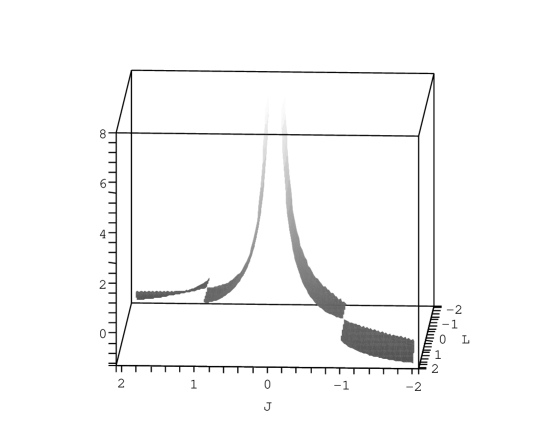
Figure 1: 3d plot of $\sqrt{x_{ctc}}-\sqrt{x_{+}}$ in terms of $L$ and $J$.(i.e. compares location of the CTC horzion to largest black hole horizon)  Note: Regions when $J^{2}>1$ are negative which means the CTC horizon is inside the black hole horizon.  The peak at $J=0$ corresponds to the infinite ctc horizon and indicates regular 5d Kerr.

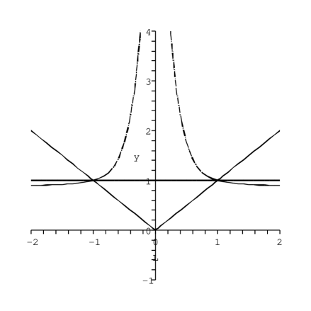
Figure 2: Plots of $\sqrt{x_{ctc}},\sqrt{x_{-}},\sqrt{x_{+}}$ it terms of $L$ and when $J=-L$, Note: dashed line corresponds to $\sqrt{x_{ctc}}$ and solid lines are $\sqrt{x_{-}},\sqrt{x_{+}}$.  Notice the CTC is horizon is either outside both horizons or inside both horizons but never in between.

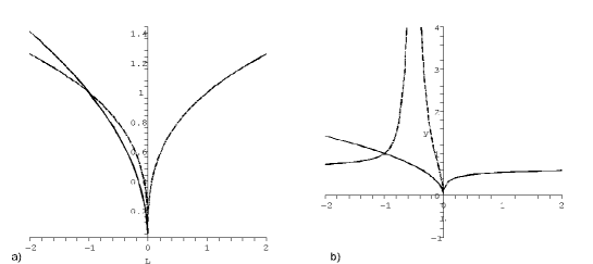
Figure 3: Plots of $\sqrt{x_{ctc}},\sqrt{x_{-}},\sqrt{x_{+}}$ it terms of a) $L$ when $J=1$ b) $L$  when $J=-2L-1$ Note: the dashed line corresponds to $\sqrt{x_{ctc}}$ and solid lines are $\sqrt{x_{-}},\sqrt{x_{+}}$ (These are extremal cases so $\sqrt{x_{-}}=\sqrt{x_{+}}$ ) Notice, black hole horizons do not exist for a) when $L>0$ and b) when $L>0$.  Also in b) $\sqrt{x_{ctc}}$ is infinite at $L=-\frac{1}{2}$ because. $J=0$ which is 5d Kerr.

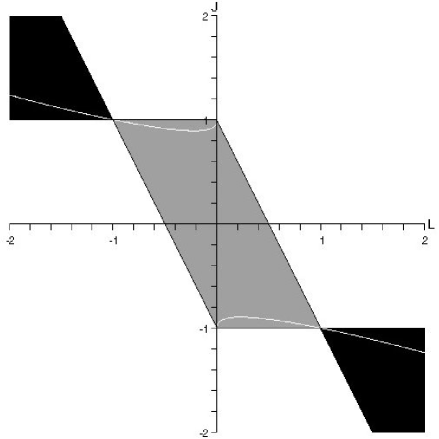
Figure 4: Plot of the horizon behavior in terms of $J$ and $L$.  The white region corresponds to naked singularities (no black hole horizons).  In the grey region the CTC horizon is outside both black hole horizons.  In the black region the CTC horizon is inside both black hole horizons.  The white line corresponds to the special case when the CTC horizon is in coincidence with a black hole horizon (outer horizon in grey region, inner horizon in black region, and both at the special points $J=-L=\pm 1$)

We claim that is not possible to have the CTC horizon located in between the two black hole horizons. Assuming the contrary, consider the problem of finding values of $J$ and $L$ when the CTC horizon is in between the two black hole horizons.  We first look for solutions when the CTC horizon is in coincidence with one of the black hole horizons.  We find that $x_{ctc}=x_{\pm}$ when the equation

$$(3J^{2}+2JL-2)^{2}+4J^{2}-5J^{4}=0$$ (10)

holds. Notice that $J=-L=\pm 1$ are solutions to (10).

An analysis of the curve resulting from the left-hand-side of (10) indicates that when both $J^{2}<1$ and $L^{2}<1$ then the CTC horizon is coincident with the outer horizon; on either side of this curve the CTC horizon is outside both black hole horizons. When both $J^{2}>1$ and $L^{2}>1$ then the CTC horizon is coincident with the inner horizon, and on either side of this curve the CTC horizon is inside both $r_{+}$ and $r_{-}$.   In all other regions of   parameter space the metric (4) has naked singularities. Figure 4  illustrates this behavior in terms of $J$ and $L$.  In the grey region the CTC horizon is outside both black hole horizons.  In the black region the CTC horizon is inside both $r_{+}$ and $r_{-}$.  The white line corresponds to the curves resulting from (10). In the white region the metric has no black hole horizons and naked singularities are present.

An alternate verification for the fact that the CTC horizon is never in between the black hole horizons may be obtained by substituting $x_{\pm}$ into $g(x)$, which shows that when $J^{2}<1$ then $g(x_{-})>0,g(x_{+})\geq 0$ and for $J^{2}>$ $1$ then $g(x_{-})\leq 0,g(x_{+})<0$ (plots not shown).  Conceptually it is easy to see why this property must be true by looking at the definition (3) of the function $g(r)$, which defines where the CTC horizon must be located.  If $r=r_{ctc}$ then $g(r_{ctc})=0$ which implies $r_{ctc}^{2}V(r_{ctc})=4a^{2}(r_{ctc})$.  For this equality to be true then $V(r_{ctc})$ must be positive since every other term in the equation is positive.  Since $V(r_{ctc})$ cannot be negative then $r_{ctc}$ cannot be in between $r_{-}$ and $r_{+}$.

Another property worth mentioning is the location of the black hole horizons in relation to $x=1$ (ie. the ergosphere $r=\sqrt{2m}$).  When $J^{2}<1$ then $x_{\pm}\leq 1$ so the horizons are inside the ergosphere. When $J^{2}>1$ then $x_{\pm}\geq 1$ so the “horizons” are outside the ergosphere. Indeed when $J^{2}>1$ the surfaces $x_{\pm}=1$ are not actually horizons, though we have been using this term as a counterpart to the $J^{2}<1$ case. Henceforth we shall refer to this as the “other region” of parameter space.

Our finding that the CTC horizon can never be in between the two black hole horizons is contrary to assumptions made in previous work [14]. However the resultant thermodynamics is not significantly altered, as all main results consider only the situation when the CTC horizon is outside the black hole.  In the next two sections we will discuss the properties of the black hole region and the other region of parameter space.   

3.2 Black Hole region of parameter space ($J^{2}<1$)

This is the region that is well understood and can be simply regarded as a Kerr Black Hole embedded in a Gödel space time, with the CTC horizon outside of the black hole horizons. To better understand this case we will take a look at the geodesics in the $(t,r,\phi)$ plane (with $\theta$ and $\psi$ fixed). The metric becomes

$$ds^{2}=-\frac{r^{2}V(r)}{4g(r)}dt^{2}+g(r)(d\phi-\frac{a(r)}{g(r)}dt)^{2}+\frac{dr^{2}}{V(r)}$$ (11)

Note that $g(r_{H})\geq 0$ for the choice of parameters $(-1\leq J\leq 1,-\frac{1}{2}-\frac{J}{2}\leq L\leq\frac{1}{2}-\frac{J}{2})$ that we are considering. For convenience we impose the further restriction that $L\neq\frac{-3J^{2}+2+\sqrt{5J^{4}-4J^{2}}}{2J}$ and $L\neq\frac{-3J^{2}+2-\sqrt{5J^{4}-4J^{2}}}{2J}$ so that $g(r_{H})>0$ and the CTC horizon is strictly outside the outer black hole horizon.

The tangent vector to a geodesic is given by:

$$u^{\alpha}=[\dot{t},\dot{r},\dot{\phi}]$$

where dot denotes the derivative with respect to the affine parameter $\lambda$.  For this metric $\partial_{t}$ and $\partial_{\phi}$ are Killing vectors so in general the energy and angular momentum for these geodesics are respectively

$$E = \frac{r^{2}V(r)-4a^{2}(r)}{4g(r)}\dot{t}+a(r)\dot{\phi}$$

$$\ell = -a(r)\dot{t}+g(r)\dot{\phi}$$

We are interested in geodesics with $\ell=0$.  Note that for constant $r$ the quantity $d\chi=d\phi-\frac{a(r)}{g(r)}dt$ is constant (i.e. $\frac{d\chi}{d\lambda}=0$); for $r=r_{H}$ these correspond to geodesics for which $\chi=\phi-\Omega_{H}t$ is constant on the horizon (recall $\Omega_{H}=\frac{a(r_{H})}{g(r_{H})}$).

Setting $\ell=0$ yields $\frac{a(r)}{g(r)}$ $\dot{t}=\dot{\phi}$ and $E=\frac{r^{2}V(r)}{4g(r)}\dot{t}$. For null geodesics we find $\dot{r}=\pm\frac{rV(r)}{2\sqrt{g(r)}}\dot{t}$, so that

$$u_{\pm}^{\alpha}=K_{\pm}\left[\frac{g(r)}{V(r)r^{2}},\pm\frac{\sqrt{g(r)}}{2r},\frac{a(r)}{V(r)r^{2}}\right]$$ (12)

where the plus/minus signs refer to outgoing/ingoing geodesics. When $l=0$ this can be solved explicitly, and we recover the results for geodesic motion examined in ref. [4]. The $K_{\pm}$’s are constants related to the energy $E=\frac{K_{\pm}}{4}$. Choosing the normalization

$$g_{\alpha\beta}u_{+}^{\alpha}u_{-}^{\beta}=-1$$

at some point $r=r_{0}$, we obtain

$$K_{+}K_{-}=\frac{2r_{0}^{2}V(r_{0})}{g(r_{0})}$$

and for convenience we pick $K_{-}=1,K_{+}=\frac{2r_{0}^{2}V(r_{0})}{g(r_{0})}$. The expansion scalar for null geodesics is

$$\Theta(u_{\pm})=\pm\frac{K_{\pm}g^{\prime}(r)}{4r\sqrt{g(r)}}$$

and we see that for outgoing null rays there is a sign difference between geodesics starting inside the horizon ($r_{0}<r_{H})$ and geodesics starting outside ($r_{0}>r_{H}$), with no such change for ingoing geodesics, as expected for a trapped surface at $r=r_{H}$.

We can also say useful things about  the CTC boundary. It occurs when $g(r_{ctc})=0$, so the expansions are infinite there. Furthermore $\frac{dr}{dt}$ is infinite and $\frac{dr}{d\lambda}=0$ there, implying that null geodesics cannot cross the CTC boundary. These results are consistent with the observations for the Schwarzschild-Gödel ($l=0$) case [4]: null geodesics will take infinite coordinate time $t$ to go between the black hole horizon and CTC boundary. The CTC boundary is reached in finite affine parameter $\lambda$ although once the null ray reaches the CTC horizon it spirals back toward the black hole. 

3.3 The Other Region of Parameter Space ($J^{2}>1$)

When $x_{ctc}<x_{-}$, i.e. the CTC boundary is the innermost surface, it is unclear what sort of object we now have. For convenience we shall continue to use the term horizon to signify $x_{\pm}$, and the term ergosphere to denote the surface $x=1$ ($r=\sqrt{2m}$), mindful of potential abuses of language. Both horizons are now outside of the ergosphere, but the CTC boundary can either be inside or outside of this surface, depending on the choice of parameters. For example for $J=1.5,L=-2$, $x_{ctc}>1$ (and $x_{ctc}<x_{-}<x_{+}$) but $x_{ctc}<1$ for $J=2,L=-2$.

To understand the causal properties of this spacetime we shall consider the metric for fixed $\theta$ and $\psi$ for convenience.  Consider the behavior of

$$ds^{2} = -\frac{r^{2}V(r)}{4g(r)}dt^{2}+g(r)(d\phi-\frac{a(r)}{g(r)}dt)^{2}+\frac{dr^{2}}{V(r)}$$ (13)

$$= \frac{r^{2}V(r)}{4\left|g(r)\right|}dt^{2}-\left|g(r)\right|(d\phi+\frac{a(r)}{\left|g(r)\right|}dt)^{2}+\frac{dr^{2}}{V(r)}$$

where in the outer region $r>r_{+}$ we see that $g(r)<0$ and $V(r)>0$, and so we have rewritten the metric for fixed $\left(\theta,\psi\right)$ in the 2nd line above. For $r_{-}<r<r_{+}$ then $g(r)<0$ and $V(r)<0$.

We can define a new coordinate $\chi=\phi-\frac{a(r_{0})}{g(r_{0})}t$  for some $r_{0}>r_{+}$ and the metric is now

$$ds^{2} = (-f(r)+g(r)\Omega^{2}-2a(r)\Omega)dt^{2}+2(g(r)\Omega-a(r))dtd\chi$$

$$+g(r)d\chi^{2}+\frac{dr^{2}}{V(r)}$$

where $\Omega=\frac{a(r_{0})}{g(r_{0})}$. For a fixed value of $r=r_{0}>r_{+}$ this metric simplifies to:

$$ds^{2}=+\frac{r_{0}^{2}V(r_{0})}{4\left|g(r_{0})\right|}dt^{2}-\left|g(r_{0})\right|d\chi^{2}$$ (15)

Since $g_{tt}>0,g_{\chi\chi}<0$ we see that $\chi$ functions as the time coordinate, but only near $r=r_{0}$.  For any given $r_{0}>r_{+}$ it is possible to choose such a time coordinate $\chi$ in a neighbourhood of $r_{0}$ and the metric always has signature $\left(-++++\right)$.

When $r_{-}<r<r_{+}$ the signature of the metric becomes $\left(---++\right)$  and so this region is not a physical spacetime.  There is no choice of coordinate transformation that will allow the metric to have correct signature. This is easily seen by expanding the metric near $r_{+}$ 

$$ds^{2} = +\frac{r_{+}^{2}V^{\prime}(r_{+})}{4\left|g(r_{+})\right|}(r-r_{+})dt^{2}+2\left(g^{\prime}(r_{+})\Omega_{+}-a^{\prime}(r_{+})\right)(r-r_{+})dtd\chi$$

$$-\left|g(r_{+})\right|d\chi^{2}+\frac{dr^{2}}{V^{\prime}(r_{+})(r-r_{+})}$$

indicating that the metric changes signature as $r$ passes through $r_{+}$ from above.  There is a conical singularity at $r=r_{+}$ that is removed by imposing a periodicity on $t$ of  $\frac{r_{+}V^{\prime}(r_{+})}{8\pi\sqrt{|g(r_{+})|}}$. Hence the region $r>r_{+}$ is a regular spacetime everywhere permeated by closed timelike curves due to the periodicity of $\phi$ and $t$.

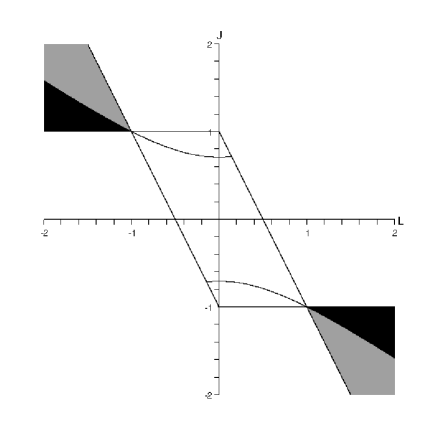
Figure 5: Plot of of horizon behavior in terms of $J$ and $L$.  Curve corresponds to $r_{ctc}=\sqrt{2m}$.  In the black region $r_{ctc}>\sqrt{2m}$ and in the grey region $r_{ctc}<\sqrt{2m}.$

Setting now $r<r_{-}$ we need to consider two distinct cases depending on where the “ergosphere” ($r_{ergo}=$ $\sqrt{2m}$) is located with respect to the CTC horizon.  These are $r_{ergo}<r_{ctc}<r_{-}$ (represented by the black region in figure 5 in terms of $L$ and $J$ parameters)  and $r_{ctc}<r_{ergo}<r_{-}$ (represented by the grey region in figure 5 in terms of $L$ and $J$ parameters).

We will start with the $r_{ergo}<r_{ctc}<r_{-}$ case and we will restrict ourselves to CTC region $r_{ctc}<r<r_{-}$ so that $g(r)<0$ and $V(r)>0$. So for this case the metric is once again in the same form as  (13).  It is possible for an arbitrary $r_{0}$ ($r_{ctc}<r_{0}<r_{-}$) to choose a coordinate $\chi=\phi-\frac{a(r_{0})}{g(r_{0})}t$ and the metrics (3.3) and (15) will be valid in this region.  Expanding the metric near $r_{-}$ gives

$$ds^{2} = +\frac{r_{-}^{2}|V^{\prime}(r_{-})|}{4\left|g(r_{-})\right|}(r_{-}-r)dt^{2}-2\left(g^{\prime}(r_{-})\Omega_{-}-a^{\prime}(r_{-})\right)(r_{-}-r)dtd\chi$$

$$-\left|g(r_{-})\right|d\chi^{2}+\frac{dr^{2}}{|V^{\prime}(r_{-})|(r_{-}-r)}$$

again showing that when $r_{-}<r<r_{+}$ the signature of the metric becomes $\left(---++\right)$. Removal of the conical singularity at $r=r_{-}$ is achieved by imposing a periodicity on $t$ of  $\frac{r_{-}|V^{\prime}(r_{-})|}{8\pi\sqrt{|g(r_{-})|}}$.  Notice that this differs from that imposed in the $r>r_{+}$ region, as expected for two regions that are disconnected spacetimes.  Referring back to (3.3), for an arbitrary choice of $\chi$ we see that $g_{\chi\chi}\rightarrow 0$ as the CTC horizon is approached. At the CTC horizon $g_{tt}$ can be either positive or negative depending on the $\Omega$ that defined $\chi$.  Examining (3.3) at $r=r_{ctc}$, it is clear that $g_{tt}$ will be positive if (a) $\Omega$ has an opposite sign to $a(r_{ctc})$ (in general this will be true since $\Omega=\frac{a(r_{0})}{g(r_{0})}$ and $g(r_{0})$ is negative) and (b)$\ |\Omega|>\frac{f(r_{ctc})}{2|a(r_{ctc})|}$ (i.e. $r_{0}$ must be chosen to be close enough to $r_{ctc}$ so that this inequality will be satisfied); otherwise $g_{tt}$ will be negative at the CTC horizon.  So for an arbitrary choice of parameters $L$ and $J$ it will not be possible to choose a single coordinate $\chi$ for which one can write the metric in a form in which $\nabla t$ is spacelike everywhere between $r_{ctc}$ and $r_{-}$.  However for an arbitrary $r_{0}$ we can choose a coordinate $\chi$ so that in a neighbourhood of $r_{0}$ the metric can be written with $\nabla t$ spacelike.  

The $r_{ctc}<r_{ergo}<r_{-}$ case is a little more interesting due to the presence of the “ergosphere”.  Outside of the ergosphere the analysis remains the same as the previous $r<r_{-}$ case.  Inside the ergosphere at any given $r_{0}$ one can still choose $\chi=$ $\phi-\frac{a(r_{0})}{g(r_{0})}t$ . However when $r_{ctc}<$ $r<r_{ergo}$ it is sufficient to choose $\Omega=0$ because $f(r)$ is negative and the metric

$$ds^{2} = -f(r)dt^{2}-a(r)dtd\phi+g(r)d\phi^{2}+\frac{dr^{2}}{V(r)}$$

$$= |f(r)|dt^{2}-a(r)dtd\phi+g(r)d\phi^{2}+\frac{dr^{2}}{V(r)}$$

is such that $\phi$ is the time coordinate inside the ergosphere.

4 Temperature from Tunneling

We now examine the application of the tunnelling method to the Kerr-Gödel spacetime.  For the case when the CTC horizon is outside the black hole horizons the temperature has been previously computed by other means [12, 13], allowing us to compare these with the tunnelling results. We can also see if any tunnelling occurs from the CTC horizon.

4.1 Review of the Tunneling method

The tunnelling method is a semi-classical approach that considers a particle idealized as a spherical wave of matter emitted from inside the horizon to outside.  From the WKB approximation the tunneling probability for the classically forbidden trajectory of the s-wave from inside to outside the horizon is

$$\Gamma\propto\exp(-2\mathrm{Im}I)$$ (16)

(here h   is set equal to unity).  Expanding the action in terms of the particle energy, the Hawking temperature is recovered at linear order.  In other words for $2I=\beta E+O(E^{2})$ this gives

$$\Gamma\thicksim\exp(-2\mathop{\mathrm{I}m}I)\simeq\exp(-\beta E)$$ (17)

From this point there are two approaches that can be used to calculate the imaginary part of the action, referred to as the null geodesic method and the Hamilton-Jacobi Ansatz (refer to [22] for more details on the two approaches).  We will only use the null geodesic method in this paper. 

The imaginary part of the action for an outgoing s-wave (which follows a radial null geodesic) from $r_{in}$ to $r_{out}$ is expressed as

$$I=\int_{r_{in}}^{r_{out}}p_{r}dr=\int_{r_{in}}^{r_{out}}\int_{0}^{p_{r}}dp_{r}^{\prime}dr$$ (18)

where $r_{in}$ and $r_{out}$ are the respective initial and final radii of the black hole. The trajectory between these two radii is the barrier the particle must tunnel through.  Note the local nature of this calculation: the tunnelling probability only depends on an integration from $r_{in}$ to $r_{out}$.  In fact only the near horizon form of the black hole metric is required in order to calculate the tunneling probability (and hence the black hole temperature) [17, 22]. So a stationary observer anywhere outside the black hole would be able to observe the emission and measure the temperature.  This is in contrast with the Wick Rotation method which requires a (scalar) field at infinity to be in equilibrium with the black hole in order to get the temperature.  The presence of the CTC horizon at large distances renders the foundations of this latter approach somewhat questionable.

We assume that the emitted s-wave has energy $\omega<<M$ and that the total energy of the space-time was originally $M$. Invoking conservation of energy, to this approximation the s-wave moves in a background spacetime of energy $M\rightarrow M-\omega^{\prime}$.  In order to evaluate the integral, we employ Hamilton’s equation $\dot{r}=\frac{dH}{dp_{r}}|_{r}$ to switch the integration variable from momentum to energy ($dp_{r}=\frac{dH}{\dot{r}}$), giving

$$I=\int_{r_{in}}^{r_{out}}\int_{M}^{M-\omega}\frac{dr}{\dot{r}}dH=\int_{0}^{\omega}\int_{r_{in}}^{r_{out}}\frac{dr}{\dot{r}}(-d\omega^{\prime})$$ (19)

where $dH=-d\omega^{\prime}$ because total energy $H=M-\omega^{\prime}$ with $M$ constant. Note that $\dot{r}$ is implicitly a function of $M-\omega^{\prime}$.  Since $\omega<<M$  it is possible to rewrite the expression in terms of an expansion of $\omega$.  To first order this gives

$$I =\int_{0}^{\omega}\int_{r_{in}}^{r_{out}}\frac{dr}{\dot{r}(r,M-\omega^{\prime})}(-d\omega^{\prime})=-\omega\int_{r_{in}}^{r_{out}}\frac{dr}{\dot{r}(r,M)}+O(\omega^{2})$$

$$\simeq\omega\int_{r_{out}}^{r_{in}}\frac{dr}{\dot{r}(r,M)}$$ (20)

To proceed further we will need to estimate the last integral. First we note that $r_{in}>r_{out}$ because black holes decrease in mass as energy is emitted; consequently the radius of the event horizon decreases.  We therefore write $r_{in}=r_{H}(M)-\epsilon$ and $r_{out}=r_{H}(M-\omega)+\epsilon$ where $r_{H}(M)$ denotes the location of the event horizon of the original background space-time before the emission of particles.  Henceforth the notation $r_{H}$ will be used to denote $r_{H}(M)$. Note that with this generalization no explicit knowledge of the total energy or mass is required since $r_{H}$ is simply the radius of the event horizon before any particles are emitted.

We pause to discuss a few technical points connected with rotating spacetimes [17],[22].  In general the emitted s-wave could carry angular momentum $\ell$; if it has energy $E$ then the tunnelling probability to the lowest order would be

$$\Gamma\simeq\exp(-\beta(E-\Omega_{H}\ell))$$

where $\Omega_{H}$ is the angular velocity of the black hole horizon.  For this tunnelling probability to make sense we must require $E-\Omega_{H}\ell>0$.  This inequality corresponds to the s-wave being able to escape from the ergosphere. For calculating the temperature $\beta^{-1}$ it is sufficient to restrict to $\ell=0$ s-waves.

4.2 Temperature Calculation

Turning now to calculation of the black hole temperature [15, 28], recall that the full metric in lapse shift form is (4).  To employ the null geodesic method it is convenient to write the metric in a Painlevé form so that the null geodesic equations convey the semi-permeable nature of the black hole horizon (i.e. that it is easy to cross into the black hole but classically they cannot escape).  In order to simplify the equations we rewrite the metric by defining $\chi=\phi-\Omega_{H}t$. We are interested in geodesics that have no angular momentum ($\ell=0$) so we set $d\chi=0$ (and for convenience also $d\theta=d\psi=0$), yielding

$$ds^{2}=-\frac{r^{2}V(r)}{4g(r)}dt^{2}+\frac{dr^{2}}{V(r)}$$

We can easily rewrite this in Painlevé form via the following transformation

$$t\rightarrow t-\mathop{\displaystyle\int}\frac{2\sqrt{g(r)}}{rV(r)}\sqrt{1-V(r)}dr$$

giving (for constant $\chi,\theta,$and $\psi$) the following Painleve metric

$$ds^{2}=-\frac{r^{2}V(r)}{4g(r)}dt^{2}+\frac{r}{\sqrt{g(r)}}\sqrt{1-V(r)}drdt+dr^{2}$$

We need to know how the $\ell=0$ null geodesics behave for this metric in order to solve for the imaginary part of the action using equation (20).  The radial null geodesic equation is given by:

$$\frac{dr}{dt}=\frac{r}{2\sqrt{g(r)}}(\pm 1-\sqrt{1-V(r)})$$ (21)

where $+$ denotes outgoing and $-$ denotes ingoing geodesics (notice that $\frac{dr}{dt}=0$ at the horizon for outgoing geodesics and $\frac{dr}{dt}$ is nonzero for ingoing geodesics).  Inserting (21) into (20) we find that $1/\frac{dr}{dt}$has a first order pole at the horizon with residue $\frac{4\sqrt{g(r_{H})}}{r_{H}V^{\prime}(r_{H})}$.  So solving the integral we find:

$$\mathop{\mathrm{I}m}I = \frac{4\pi\omega\sqrt{g(r_{H})}}{r_{H}V^{\prime}(r_{H})}+O(\omega^{2})$$

$$\Gamma \thicksim \exp(-2\mathop{\mathrm{I}m}I)\simeq\exp(-\frac{8\pi\sqrt{g(r_{H})}}{r_{H}V^{\prime}(r_{H})}\omega)$$

This corresponds to a temperature:

$$T = \frac{r_{H}V^{\prime}(r_{H})}{8\pi\sqrt{g(r_{H})}}$$ (22)

$$T = \frac{m(r_{H}^{2}(1-8j^{2}m-4ml)-2l^{2})}{\pi r_{H}^{3}\sqrt{-4j^{2}r_{H}^{6}+(1-8j^{2}m)r_{H}^{4}+2ml^{2}}}$$ (23)

This temperature is the same as that obtained using Wick-rotation methods [13, 14]; when $l=0$ it reduces down to the Schwarzschild-Gödel temperature found in [12]. Note that the expression for the temperature diverges when $g(r_{H})=0$, which occurs when the CTC horizon is coincident with the outer horizon.  The temperature is not defined when $g(r_{H})<0$ , an unsurprising result considering the analysis of the other region of parameter space and the fact the when the CTC horizon is inside the $r_{-}$ and $r_{+}$ horizons the derivation used is not valid.  Not only is $t$ not the correct time coordinate, but it is unclear how to even define tunnelling from inside $r_{+}$ because the region $r_{-}<r<r_{+}$ is not a spacetime.  

Consider next what happens if we try to apply the tunnelling method to the CTC horizon.  From (21) we know that $\frac{dr}{dt}\rightarrow\infty$ as $r\rightarrow r_{ctc}$.  This means that $1/\frac{dr}{dt}$ is simply zero at the CTC horizon. Since $1/\frac{dr}{dt}$ has no poles at the CTC horizon it means there is no tunnelling at the CTC horizon.

5 Conclusions

In this paper we have reviewed some of the general properties of the Kerr-Godël spacetime, performing detailed analysis of its parameter space. There are two distinct classes. One is the class $J^{2}<1$, corresponding to black holes for which the CTC horizon $r_{CTC}$ is exterior to the black hole horizons at $r_{+}$ and $r_{-}$ . When $J^{2}>1$ we obtain the other class (the “other” region of parameter space), for which the CTC horizon is inside both of the other surfaces $r_{+}$ and $r_{-}$ .  We find that these are the only two possibilities (apart from naked singularities); there is no “in-between” region where $r_{+}>r_{CTC}>r_{-}$ , contrary to previous expectations [14].

Despite the presence of CTCs, we find that the tunnelling method applied to the black hole region of parameter space yields a temperature consistent with previous calculations made via Wick rotation methods.  We also find (when $r_{ctc}>r_{+}$ ) that there is no tunnelling through the CTC horizon.  We have discussed technical problems that occur in trying to apply the tunnelling method to the “other” region of parameter space due the fact that the region $r_{-}<r<r_{+}$ does not have the correct signature.  Higher-order corrections and applications of the method to non-radial null rays remain as interesting problems to explore.

Acknowledgements

This work was supported in part by the Natural Sciences and Engineering Research Council of Canada.

References

- [1] J. P. Gauntlett, J. B. Gutowski, C. M. Hull, S. Pakis, and H. S. Reall, ”All supersymmetric solutions of minimal supergravity in five dimensions”, Class. Quant. Grav. 20, 4587-4634 (2003)
- [2] C. A. R. Herdeiro, ”Spinning deformations of the D1-D5 system and a geometric resolution of Closed Timelike Curves”, Nucl.Phys. B665, 189-210 (2003)
- [3] E. Boyda, S. Ganguli, P. Horava, and U. Varadarajan, ”Holographic Protection of Chronology in Universes of the Godel Type”, Phys.Rev. D67, 106003 (2003)
- [4] E. G. Gimon, and A. Hashimoto, ”Black holes in Godel universes and pp-waves”, Phys. Rev. Lett. 91, 021601 (2003)
- [5] Troels Harmark, and Tadashi Takayanagi, ”Supersymmetric Godel Universes in String Theory”, Nucl. Phys. B662 (2003) 3-39
- [6] R. Biswas, E. Keski-Vakkuri, R. G. Leigh, S. Nowling, and E. Sharpe, ”The Taming of Closed Time-like Curves”, JHEP 0401 (2004) 064
- [7] D. Brecher, P. A. DeBoer, D. C. Page, and M. Rozali, ”Closed Timelike Curves and Holography in Compact Plane Waves”, JHEP 0310 (2003) 031
- [8] C. A. R. Herdeiro, ”The Kerr-Newman-Godel Black Hole”, Class. Quant. Grav. 20, 4891-4900 (2003)
- [9] D. Brace, C. A. R. Herdeiro, S. Hirano, ”Classical and Quantum Strings in compactified pp-waves and Godel type Universes”, Phys. Rev. D69 (2004) 066010
- [10] D. Brecher, U. H. Danielsson, J. P. Gregory, and M. E. Olsson, ”Rotating Black Holes in a Godel Universe”, JHEP 0311 (2003) 033
- [11] H. Takayanagi, ”Boundary States for Supertubes in Flat Spacetime and Godel Universe”, JHEP 0312 (2003) 011
- [12] D. Klemm, and L. Vanzo, ”On the Thermodynamics of Goedel Black Holes”, Fortsch. Phys. 53 919-925 (2005)
- [13] G. Barnich, and G. Compere, ”Conserved charges and thermodynamics of the spinning Godel black hole”, Phys. Rev. Lett. 95, 031302 (2005)
- [14] M. Cvetic, G.W. Gibbons, H. Lu, and C.N. Pope, “Rotating Black Holes in Gauged Supergravities; Thermodynamics, Supersymmetric Limits, Topological Solitons and Time Machines”,DAMTP-2005-39, MIFP-05-08, UPR-1114-T
- [15] P. Kraus and F. Wilczek,“A Simple Stationary Line Element for the Schwarzschild Geometry, and Some Applications” [gr-qc/9406042]; P. Kraus and F. Wilczek, “Self-Interaction Correction to Black Hole Radiance”, Nucl. Phys. B433, 403 (1995) [gr-qc/9408003]; P. Kraus and F. Wilczek, “Effect of Self-Interaction on Charged Black Hole Radiance”, Nucl. Phys. B437 231-242 (1995) [hep-th/9411219]; P. Kraus and E. Keski-Vakkuri, “Microcanonical D-branes and Back Reaction”, Nucl.Phys. B491 249-262 (1997) [hep-th/9610045]; M. K. Parikh and F. Wilczek, “Hawking Radiation as Tunneling”, Phys. Rev. Lett. 85, 5042 (2000), [arXiv:hep-th/9907001];M. K. Parikh, “New Coordinates for de Sitter Space and de Sitter Radiation”, Phys. Lett. B 546, 189, (2002) [hep-th/0204107]; M. K. Parikh, “A Secret Tunnel Through The Horizon”, Int.J.Mod.Phys. D13 2351-2354 (2004) [hep-th/0405160]; M. K. Parikh, “Energy Conservation and Hawking Radiation”, [arXiv:hep-th/0402166]; K. Srinivasan and T.Padmanabhan , “Particle Production and Complex Path Analysis”, Phys. Rev. D60 , 24007 (1999) [gr-qc-9812028]
- [16] M. Agheben, M. Nadalini, L Vanzo, and S. Zerbini, “Hawking Radiation as Tunneling for Extremal and Rotating Black Holes”, JHEP 0505 (2005) 014 [hep-th/0503081];
- [17] M. Arzano, A. Medved and E. Vargenas, “Hawking Radiation as Tunneling through the Quantum Horizon”, JHEP 0509 (2005) 037 [hep-th/0505266]
- [18] Qing-Quan Jiang, Shuang-Qing Wu, and Xu Cai, “Hawking radiation as tunneling from the Kerr and Kerr-Newman black holes”,Phys.Rev. D73 (2006) 064003 [hep-th/0512351]
- [19] Jingyi Zhang, and Zheng Zhao, “Charged particles’ tunnelling from the Kerr-Newman black hole”, Phys.Lett. B638 (2006) 110-113 [gr-qc/0512153]; Yapeng Hu, Jingyi Zhang, and Zheng Zhao, ”The relation between Hawking radiation via tunnelling and the laws of black hole thermodynamics” [gr-qc/0601018]
- [20] Liu Zhao, ”Tunnelling through black rings”, [hep-th/0602065]
- [21] Shuang-Qing Wu, and Qing-Quan Jiang, ”Remarks on Hawking radiation as tunneling from the BTZ black holes”, JHEP 0603 (2006) 079, [hep-th/0602033]
- [22] R. Kerner and R.B. Mann, “Tunnelling, Temperature and Taub-NUT Black Holes”, Phys.Rev. D73 (2006) 104010
- [23] Shuang-Qing Wu, and Qing-Quan Jiang, ”Hawking Radiation of Charged Particles as Tunneling from Higher Dimensional Reissner-Nordstrom-de Sitter Black Holes”, [hep-th/0603082]
- [24] B. D. Chowdhury, ”Tunneling of Thin Shells from Black Holes: An Ill Defined Problem”, [hep-th/0605197]
- [25] Emil T.Akhmedov, Valeria Akhmedova, Terry Pilling, and Douglas Singleton, ”Thermal radiation of various gravitational backgrounds”, [hep-th/0605137]; Emil T. Akhmedov, Valeria Akhmedova, and Douglas Singleton, ”Hawking temperature in the tunneling picture”, Phys.Lett. B642 (2006) 124-128 [hep-th/0608098]
- [26] Satoshi Iso, Hiroshi Umetsu, and Frank Wilczek, ”Anomalies, Hawking Radiations and Regularity in Rotating Black Holes”,Phys.Rev. D74 (2006) 044017 [hep-th/0606018]
- [27] Jun Ren, Jingyi Zhang, and Zheng Zhao, ”Tunnelling Effect and Hawking Radiation from a Vaidya Black Hole”, Chin.Phys.Lett. 23 (2006) 2019-2022, [gr-qc/0606066]
- [28] Zhao Ren, Li Huai-Fan, and Zhang Sheng-Li, ”Canonical Entropy of charged black hole” [gr-qc/0608123]
- [29] P. Mitra, ”Hawking temperature from tunnelling formalism”, [hep-th/0611265]