hep-th/0701087

Factorization of Seiberg-Witten Curves

with Fundamental Matter

Romuald A. Janik^a, Niels A. Obers^b and Peter B. Rønne^b

^a Institute of Physics, Jagellonian University

Reymonta 4, 30-059, Krakow, Poland

^bThe Niels Bohr Institute

Blegdamsvej 17, 2100 Copenhagen Ø, Denmark

ufrjanik@if.uj.edu.pl, obers@nbi.dk, roenne@nbi.dk

Abstract

We present an explicit construction of the factorization of Seiberg-Witten curves for ${\cal N}=2$ theory with fundamental flavors. We first rederive the exact results for the case of complete factorization, and subsequently derive new results for the case with breaking of gauge symmetry $U(N_{c})\to U(N_{1})\times U(N_{2})$. We also show that integrality of periods is necessary and sufficient for factorization in the case of general gauge symmetry breaking. Finally, we briefly comment on the relevance of these results for the structure of ${\cal N}=1$ vacua.

1 Introduction

The study of supersymmetric gauge theories has provided many new insights into non-perturbative phenomena in gauge theories. The constraints imposed by supersymmetry combined with other simplifications and symmetries have made it possible to obtain exact non-perturbative results for at least some quantities in these gauge theories. In particular, in the seminal work of Seiberg and Witten [1, 2] it was shown that the low-energy dynamics of ${\cal{N}}=2$ supersymmetric gauge theories is encoded in the properties of an associated hyperelliptic Seiberg-Witten (SW) curve.

Furthermore, remarkable progress has been made in understanding the structure of ${\cal{N}}=1$ theories obtained from breaking the ${\cal{N}}=2$ theory by turning on a superpotential for the adjoint ${\cal{N}}=1$ chiral superfield. Motivated by constructions in string theory [3], Dijkgraaf and Vafa [4] found a link between the effective superpotentials in these theories and random matrix theory, which was later understood in purely field theoretic terms [5, 6, 7]. (See e.g. Refs. [8, 9, 10, 11] for pedagogical introductions)

Much of the physics of the ${\cal{N}}=2$ theory deformed by a tree-level superpotential can be obtained effectively from the knowledge that the SW-curve of the undeformed theory factorizes, since the resulting ${\cal{N}}=1$ theories occur in the region of the ${\cal{N}}=2$ moduli space where (some) monopoles become massless. The relation of this to the matrix model conjecture of Dijkgraaf and Vafa were studied in e.g. Refs. [12, 5, 13, 14, 15, 16, 17].

In these developments one has primarily focussed on the case in which the gauge group is not broken, using factorization of the SW-curve in terms of Chebyshev polynomials as found in [18]. If one goes beyond this, and considers for example the breaking $U(N_{c})\rightarrow U(N_{1})\times U(N_{2})$ it was found [19, 20, 21] that the space of ${\cal{N}}=1$ vacua exhibits a very complex structure of various connected components, each of which allows for multiple dual descriptions of the same physics but with different patterns of breaking. While in these works one had to consider the factorization of SW-curves on a case by case basis for low $N_{c}$, Ref. [22] contains an exact solution of the factorization problem for arbitrary $N_{c}$ for any gauge breaking of the form $U(N_{c})\rightarrow U(N_{1})\times U(N_{2})$. This was then also used to further study the global structure of ${\cal{N}}=1$ vacua (see also [23]).

Although the case without flavors already exhibits a very rich structure, inclusion of flavors in the circle of ideas discussed is of physical interest and has received a lot of attention as well. In particular, matrix models methods were used in Ref. [24] to obtain a solution of the complete factorization of SW-curves for theories with fundamental flavors. See also Refs. [25, 26, 27, 28, 29, 30, 31] for work on the relation to the matrix model in the presence of fundamental matter. Following the work [19] the phase structure of ${\cal{N}}=1$ theories with fundamental matter was then explored in Refs. [32, 33, 34, 35, 36]. Also here, one is confined to considering specific cases with low $N_{c}$ and low number of flavors $N_{f}$

The purpose of this paper is to extend the factorization of the SW-curve for the gauge breaking $U(N_{c})\rightarrow U(N_{1})\times U(N_{2})$ found in [22] to the case when fundamental matter is included in the ${\cal{N}}=2$ supersymmetric $U(N_{c})$ gauge theory. An exact expression of the factorization of the SW-curve in this genus one case is obtained for arbitrary $N_{c}$ and $0\leq N_{f}<2N_{c}$. The construction includes the genus one case of [22] for $N_{f}=0$. Furthermore, it correctly reduces to the genus zero case with flavors in the fundamental, reproducing the results of Ref. [24] in a simpler way. As an important ingredient we prove that integrality of periods is necessary and sufficient for factorization in the case of general gauge symmetry breaking.

The structure of the paper is as follows. In Section 2 we briefly review some useful facts about ${\cal{N}}=2$ supersymmetric QCD for $U(N_{c})$ gauge theory with $N_{f}$ flavors transforming in the fundamental, including the corresponding SW-curve. Section 3 presents the factorization of the SW-curve, and defines in particular the problem of the factorization when $N_{c}-2$ monopoles in the low energy effective action become massless. This corresponds to the gauge group breaking $U(N_{c})\rightarrow U(N_{1})\times U(N_{2})$ and the physics will only depend on a reduced curve which is elliptic, i.e has genus one. In Section 4 we summarize the equations that the meromorphic one-form needs to obey in order to solve the factorization problem. We then consider in Section 5 first the genus zero case of complete factorization, where we rederive in a very simple way the original results of [24].

Section 6 then contains the main result of the paper, namely the exact solution of the factorization of the SW-curve in the genus one case when fundamental matter is present. We end with the conclusions and open problems in Section 7. Two appendices are included. In Appendix A we prove the statement that a necessary and sufficient condition for factorization of the SW-curve is integrality of the periods as specified in Section 3. Appendix B considers the general solution of Section 6 when flavors are decoupled, reproducing the genus one solution of [22].

2 $\mathcal{N}=2$ SQCD

We consider an $\mathcal{N}=2$ supersymmetric $U(N_{c})$ gauge theory with $N_{f}$ flavors, i.e. we add the following terms to the pure $\mathcal{N}=2$ SYM Lagrangian for the (adjoint) chiral superfield, $\Phi$ [37]

$$\int\!\mathrm{d}\theta^{4}\left(Q^{\dagger}_{i}e^{-2V}Q_{i}+\widetilde{Q}_{i}e^{-2V}\widetilde{Q}^{\dagger}_{i}\right)+\int\!\mathrm{d}\theta^{2}\left(\sqrt{2}\widetilde{Q}_{i}\Phi Q_{i}+\sqrt{2}\widetilde{Q}_{i}M_{ij}Q_{j}\right)+\mathrm{h.c.}\ .$$ (2.1)

Here we have suppressed the gauge indices, and $Q_{i}$ ($\widetilde{Q}_{i}$) are chiral superfields transforming in the (anti-)fundamental representation of $U(N_{c})$. The flavor index $i$ runs from 1 to $N_{f}$. The mass matrix fulfills $[M,M^{\dagger}]=0$ so it can be diagonalized [38] by a rotation in flavor-space. Denoting the eigenvalues of the mass matrix as $m_{i}$, the superpotential in (2.1) takes the form

$$\sqrt{2}\widetilde{Q}_{i}\Phi Q_{i}+\sqrt{2}m_{i}\widetilde{Q}_{i}Q_{i}.$$ (2.2)

The object of our interest is the vacuum moduli space for the Coulomb phase of the theory where, classically, we have zero expectation values for the quarks, $\Phi$ is diagonal, and its eigenvalues $\phi_{a}$ parameterize the moduli space. Generically, $U(N_{c})$ breaks down to $U(1)^{N_{c}}$ but if some of the eigenvalues $\phi_{a}$ coincide we get non-abelian factors. Further, if $\phi_{a}+m_{i}=0$ we get a massless quark. Quantum mechanically, the vacuum moduli space is $N_{c}$-dimensional and parameterized by

$$u_{k}=\frac{1}{k}\left<\operatorname{Tr}\Phi^{k}\right>,\quad k=1,\ldots,N_{c}\ .$$ (2.3)

These are encoded in the polynomial

$$P_{N_{c}}(x,u_{k})=\left<\mathrm{det}(xI-\Phi)\right>=x^{N_{c}}+\sum_{i=1}^{N_{c}}s_{i}x^{N_{c}-i}\ ,$$ (2.4)

where the coefficients, $s_{i}$, are polynomials in the $u_{k}$’s and the relation is given by Newton’s formula

$$is_{i}+\sum_{k=1}^{i}ks_{i-k}u_{k}=0,\qquad i=0,\ldots,N_{c}\ ,$$ (2.5)

where we define $s_{0}\equiv 1$.

As is well-known, without fundamental matter the low energy effective description of the theory is beautifully captured by a one-form on a hyperelliptic curve, the Seiberg-Witten (SW) curve, of genus $N_{c}-1$ [1, 2]. In the case with fundamental matter, the SW-curve takes the form

$$y^{2}=P_{N_{c}}(x,u_{k})^{2}-4\Lambda^{2N_{c}-N_{f}}\prod_{i=1}^{N_{f}}(x+m_{i}),\qquad N_{f}<2N_{c}\ ,$$ (2.6)

where $m_{i}$ are the bare masses from (2.2). This was first found for the $\mathrm{SU}(2)$ gauge group (see [2] and references therein) and later for general $\mathrm{SU}(N)$ gauge groups in [38, 39]. For $N_{f}\geq N_{c}$ the curve is, however, ambiguous and we can add a polynomial to $P_{N_{c}}$ without changing the prepotential of the low-energy effective theory (see Refs. [39, 40]) (for $N_{c}\leq N_{f}<2N_{c}$)

$$y^{2}=(P_{N_{c}}(x,u_{k})+\Lambda^{2N_{c}-N_{f}}Q_{N_{f}-N_{c}}(x,m_{i},\Lambda))^{2}-4\Lambda^{2N_{c}-N_{f}}\prod_{i=1}^{N_{f}}(x+m_{i})\ ,$$ (2.7)

where $Q_{N_{f}-N_{c}}$ is a polynomial of degree $N_{f}-N_{c}$ independent of the $u_{k}$’s.

In this paper we will use the SW-curve in the form (2.6). Note that we can lower the value of $N_{f}$ with one unit by taking the limit $m_{i}\rightarrow\infty,\,\Lambda\rightarrow 0$ for a given $i$ while keeping $\Lambda^{2N_{c}-N_{f}}m_{i}\equiv\Lambda_{\rm new}^{2N_{c}-(N_{f}-1)}$ constant. This corresponds to removing the $i$th flavor and the new scale $\Lambda_{\rm new}$ is obtained by scale matching. In this way one can find the remaining curves for lower $N_{f}$, given the curve for $N_{f}=2N_{c}$, by taking the appropriate limits [38]. In particular, using this procedure one can also obtain the curve without fundamental matter. The constraint $N_{f}<2N_{c}$ is needed for the theory to be asymptotically free (see e.g. [41]) and the metric on our moduli space will otherwise not be positive definite for large $\Phi$ [32].

3 Factorization

We will investigate submanifolds of the moduli space where the SW-curve factorizes, i.e. it takes the form

$$y^{2}=P_{N_{c}}(x,u^{({\rm fact})}_{k})^{2}-4\Lambda^{2N_{c}-N_{f}}\prod_{i=1}^{N_{f}}(x+m_{i})=F_{2(N_{c}-n)}(x)H_{n}(x)^{2}\ ,$$ (3.1)

where $F_{2(N_{c}-n)}$ and $H_{n}$ are polynomials of degree $2(N_{c}-1)$ and $n$, respectively. Here $n$ denotes the number of double roots for the curve. We will assume there are no multiple roots in $F_{2(N_{c}-n)}$ and $H_{n}$ and that they have no common roots, i.e. we have no roots of order higher than two. As in the case without fundamental matter, we expect that the solution for a given $n$ should constrain $n$ of the $N_{c}$ free parameters so we end up with $N_{c}-n$ continuous parameters. However, the subspace of factorized solutions is not invariant under translations of $x$ as in the case without matter, since such a translation would simply change the masses $m_{i}$. We thus have to look for this continuous parameter elsewhere.

These points of factorization are of special interest since here $n$ of the ${N_{c}-1}$ monopoles in the low energy effective action become massless. Importantly, these are the points we will be localized at when we softly break the $\mathcal{N}=2$ supersymmetry to $\mathcal{N}=1$ by addition of a tree-level superpotential for $\Phi$. Here the gauge groups breaks into $N_{c}-n$ parts.

In the case without fundamental matter and complete factorization, i.e. when $n=N_{c}-1$ and we only have two single roots, the problem was solved in Ref. [18] using Chebyshev polynomials. This case corresponds to an unbroken gauge group in the low energy effective theory. If we have $n=N_{c}-2$, i.e. four single roots, the general factorization was obtained using the elliptic theta function in [22] (see also [23]).

Including fundamental matter the complete factorization case was solved in [24] (see also [42] and [11]). In this paper we will solve the $n=N_{c}-2$ case where we have four single roots following closely the approach in [22]. In this case the factorization (3.1) takes the form

$$y^{2}=P_{N_{c}}(x,u^{({\rm fact})}_{k})^{2}-4\Lambda^{2N_{c}-N_{f}}\prod_{i=1}^{N_{f}}(x+m_{i})=F_{4}(x)H_{N_{c}-2}(x)^{2}\ .$$ (3.2)

The solution should be parameterized by 2 continuous parameters and a set of discrete parameters, as we indeed will see. Importantly, the physics will only depend on the reduced curve [12]

$$y_{\rm red}^{2}=F_{4}(x)\ ,$$ (3.3)

which is elliptic, i.e. has genus one, and is represented by a torus. Due to the square in (3.3) we can, as usual, see the curve as represented by two sheets connected by two cuts between the four roots of $F_{4}$. The sheets are compactified by adding points at the infinities thus giving us a torus. On this torus we have a canonical homology basis consisting of the cycles $\alpha$ and $\beta$. See Figure 1 where the cuts also are shown.

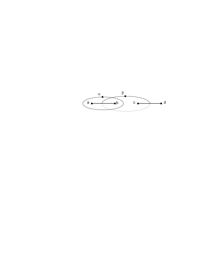
Figure 1: The figure shows the cycles and cuts for the elliptic curve. We assume that $F_{4}(x)=(x-a)(x-b)(x-c)(x-d)$. The $\alpha$ and $\beta$ cycles are shown. A dotted line means that the curve is on the lower sheet. Note that $\alpha$ and $\beta$ only intersect once.

4 Construction of the solution

As in Ref. [22] the idea is to consider

$$\omega\equiv T(x)\mathrm{d}x\equiv\left<\operatorname{Tr}\frac{\mathrm{d}x}{x-\Phi}\right>\ ,$$ (4.1)

which is a meromorphic one-form on the SW-curve. If we can determine $\omega$ we have, in principle, solved the problem since the $u_{k}$’s can then be obtained to any order using the relation

$$u_{k}=-\frac{1}{k}\mathrm{res}_{x=\infty}\,x^{k}\omega\ ,$$ (4.2)

where we have defined

$$\mathrm{res}_{x=\infty}\,\frac{1}{x}\mathrm{d}x=-1\ .$$ (4.3)

As was shown in [32] $\omega$ has residue $-N_{c}$ at infinity of the upper sheet, residue $N_{c}-N_{f}$ at the infinity of the lower sheet, and residues $+1$ at $-m_{i}$ (the zeroes of $\prod_{i}(x+m_{i})$) on the lower sheet. One can just as well have some of the mass-poles on the upper sheet and still solve the factorization problem. This will then correspond to Higgs vacua rather than Coulomb vacua [32]. In the quantum theory there is no physical boundary between the two sheets.

Furthermore, $\omega$ has integral periods

$$\frac{1}{2\pi i}\int_{\alpha}\omega=N_{1},\quad\frac{1}{2\pi i}\int_{\beta}\omega=\Delta k\ ,$$ (4.4)

where $N_{1}$ and $\Delta k$ are integers, and we have to think of definite curves for $\alpha$ and $\beta$ only encircling the cuts and not any of the poles of $\omega$. The integrality of the periods is a necessary and sufficient condition for the factorization of the SW-curve as will be made precise and proven in Appendix A. This is actually independent of the number of cuts in the factorization. As was also shown in [32] this means that $\omega$ takes the form

$$\omega=\mathrm{d}\log(P_{N_{c}}(x)+y(x))=\bigg{(}\frac{P^{\prime}_{N_{c}}(x)}{y(x)}+\frac{B^{\prime}(x)}{2B(x)}-\frac{P_{N_{c}}(x)B^{\prime}(x)}{2y(x)B(x)}\bigg{)}\mathrm{d}x\ ,$$ (4.5)

where we have defined $B(x)=\prod_{i}(x+m_{i})$. Here the residues can easily be checked and the integral periods follows from $\omega$ being the derivative of a logarithm. From (4.5) we see that not only can we retrieve the $u_{k}$’s from $\omega$ but we can also get $\Lambda$:

$$\int_{\widetilde{\Lambda_{0}}}^{\Lambda_{0}}\omega=-\log(\Lambda^{2N_{c}-N_{f}})+\log(\Lambda_{0}^{2N_{c}-N_{f}})+\mathcal{O}\!\left(\frac{1}{\Lambda_{0}}\right),$$ (4.6)

where we think of $\Lambda_{0}$ ($\widetilde{\Lambda_{0}}$ is the corresponding point on the lower sheet) as a large cut-off for the integration $\int_{\infty_{-}}^{\infty_{+}}\omega$. Here $\infty_{\pm}$ refers to the infinities on the upper/lower sheet.

Before we proceed to the genus one case which is the main focus of this paper let us exhibit the construction in the simpler case of genus zero (no gauge symmetry breaking), where we rederive in a very simple way the factorization formulas of Ref. [24].

5 Genus zero case

In the genus zero case we have $N_{c}-n=1$ and we expect a single continuous parameter in the solution.

Let us start from the reduced curve which in this case is given by the equation

$$y^{2}=F_{2}(x)\equiv(x-a)(x-b)\ .$$ (5.1)

As explained in the previous section, we have to construct a meromorphic 1-form $\omega$ on the curve with residues $-N_{c}$ at infinity on the physical sheet, $N_{c}-N_{f}$ at infinity on the second sheet and with residue 1 at $x=-m_{i}$.

It turns out to be much easier to use an unconstrained parametrization of the reduced curve, i.e. to pass to the universal covering space.

Parametrization and $\mathbb{Z}_{2}$ map.

Since the curve (5.1) has genus zero, it can be parameterized by functions on a sphere, which is represented as a compactified complex plane. This can be done very easily. Let us first rewrite the equation (5.1) in the form

$$y^{2}=(x-T)^{2}-4R\ ,$$ (5.2)

where we used the notation of [24]

$$T=\frac{a+b}{2}\quad,\quad R=\frac{(a-b)^{2}}{16}\ .$$ (5.3)

Then a rational parameterization is

$$x=T+2\sqrt{R}\frac{1+z^{2}}{1-z^{2}}\quad,\quad y=2\sqrt{R}\frac{2z}{1-z^{2}}\ .$$ (5.4)

For our application we have to keep track of some additional structure on the curve. Firstly, we have to single out points on the sphere $\infty_{+}$, $\infty_{-}$ which correspond to points at infinity in the $(x,y)$ plane. Here these are $z=\pm 1$. Secondly, it is convenient to exhibit the $\mathbb{Z}_{2}$ covering transformation which exchanges the sheets $(x,y)\to(x,-y)$. In terms of the $z$ coordinate it is represented as $z\to-z$. Its fixed points are exactly the branch points of the curve (5.1). These are $z=0$ and $z=\infty$ and correspond to $x=T+2\sqrt{R}$ and $x=T-2\sqrt{R}$ respectively.

The meromorphic 1-form

Using the $z$ coordinate we can at once write the unique meromorphic 1-form with the prescribed poles and residues

$$\omega=\left(\frac{-N_{c}}{z-1}+\frac{N_{c}-N_{f}}{z+1}+\sum_{i=1}^{N_{f}}\frac{1}{z+z_{m_{i}}}\right)dz\ ,$$ (5.5)

where the location of the pole corresponding to $x=-m$ can be found to be

$$z_{m}=\pm\frac{\sqrt{(m+T)^{2}-4R}}{m+T-2\sqrt{R}}\ .$$ (5.6)

The two choices of sign correspond to putting the pole on either of the two sheets. Since all parameters are complex we can always analytically continue the answer from one sheet to the other one. As mentioned above, this has the interpretation of interpolating between Coulomb and Higgs vacua.

Factorization solution

We can now calculate the $u_{k}$’s using (4.2). Remarkably enough all the formulas from [24] (compare e.g. formulas (38)-(40) in [42]) now follow from the simple formula

$$u_{k}=-\frac{1}{k}\mathrm{res}_{x=\infty}\,x^{k}\omega=-\frac{1}{k}\mathrm{res}_{z=1}\left(T+2\sqrt{R}\frac{1+z^{2}}{1-z^{2}}\right)^{k}\cdot\omega\ .$$ (5.7)

The final ingredient is the calculation of $\Lambda$. We use formula (4.6) in the form:

$$\log\Lambda^{2N_{c}-N_{f}}=-\lim_{\varepsilon\to 0}\left\{\int_{-1+\varepsilon}^{1-\varepsilon}\omega-N_{c}\log x(1-\varepsilon)-(N_{c}-N_{f})\log x(-1+\varepsilon)\right\}\ .$$ (5.8)

After a brief calculation one gets

$$\Lambda^{2N_{c}-N_{f}} = R^{N_{c}-\frac{N_{f}}{2}}\bigg{(}\frac{\sqrt{(m+T)^{2}-4R}-m-T+2\sqrt{R}}{\sqrt{(m+T)^{2}-4R}+m+T-2\sqrt{R}}\bigg{)}^{N_{f}}$$ (5.9)

$$= \frac{R^{N_{c}}}{\prod_{i=1}^{N_{f}}\frac{1}{2}\left(m+T+\sqrt{(m+T)^{2}-4R}\right)}\ ,$$

which is exactly the formula obtained from matrix models in [24]. Plugging these parameters into the SW-curve will lead to a complete factorization regardless of whether the flavor poles are on a single or on different sheets (which amounts to a choice of the signs of the relevant square-roots). Equation (5.9) exactly gives one constraint so we end up with one continuous parameter as expected.

Number of vacua

Finally, let us discuss the number of such vacua. From the above construction one can obtain a discrete set of $2N_{c}-N_{f}$ vacua in the following manner. Let us rescale the parameters by

$$T\to e^{i\alpha}T\quad,\quad R\to e^{2i\alpha}R\quad,\quad m\to e^{i\alpha}m\ .$$ (5.10)

Then $x$ is effectively rescaled as $x\to e^{i\alpha}x$. In order for the resulting factorization to be related to the same theory, $\Lambda^{2N_{c}-N_{f}}$ should be unchanged hence

$$\alpha=2\pi\frac{k}{2N_{c}-N_{f}}\quad,\quad k=0,\ldots,2N_{c}-N_{F}-1\ ,$$ (5.11)

which proves the claim.

6 Genus one case

Let us now adopt the same strategy in our main case of interest i.e. the genus one case. This case is especially interesting as, in contrast to the genus zero described above, there is gauge symmetry breaking, one has additional discrete parameters labelling the vacua (inequivalent factorizations), new types of Coulomb vacua appear with increasing $N_{c}$ which cannot be induced from those with smaller $N_{c}$. Even more interestingly, differing discrete labels like $(N_{1},N_{2},\Delta k,k)\neq(N^{\prime}_{1},N^{\prime}_{2},\Delta k^{\prime},k^{\prime})$ may lead to the same factorized SW-curves thus allowing for dual descriptions of the same physics.

Here we start from the reduced curve which in this case is given by the quartic equation

$$y^{2}=F_{4}(x)\equiv(x-a)(x-b)(x-c)(x-d)\ .$$ (6.1)

Note that for cubic superpotentials $W(x)$ relevant to this case the right hand side can be written as $F_{4}(x)=W^{\prime}(x)^{2}-f(x)$ with $f(x)$ a linear polynomial.

Parametrization and $\mathbb{Z}_{2}$ map.

Since the above curve is quartic, it has genus one and hence can be parameterized by a torus i.e. the complex plane modulo $(1,\tau)$, where $\tau$ is a complex parameter (the modulus) with positive imaginary part.

Again we would like to exhibit the $\mathbb{Z}_{2}$ covering map (the hyperelliptic involution) moving between the two branches of (6.1). A convenient choice is

$$z\to 1+\tau-z\ .$$ (6.2)

There are four fixed points on the torus: $0$, $1/2$, $\tau/2$ and $1/2+\tau/2$ which under the embedding $x(z)$, which we will soon give explicitly, go over to the branch points of (6.1).

Next we need to mark the two points corresponding to the infinities on the upper and lower sheet – these will be denoted $\infty_{+}$ and $\infty_{-}$ respectively. In Figure 2 the torus is illustrated with the two marked points.

We should require that the points at infinity go to each other under the $\mathbb{Z}_{2}$ covering map thus giving the relation

$$\infty_{+}=1+\tau-\infty_{-}\ .$$ (6.3)

We will find that then $\infty_{-}$ will be fixed completely when constructing the meromorphic 1-form.

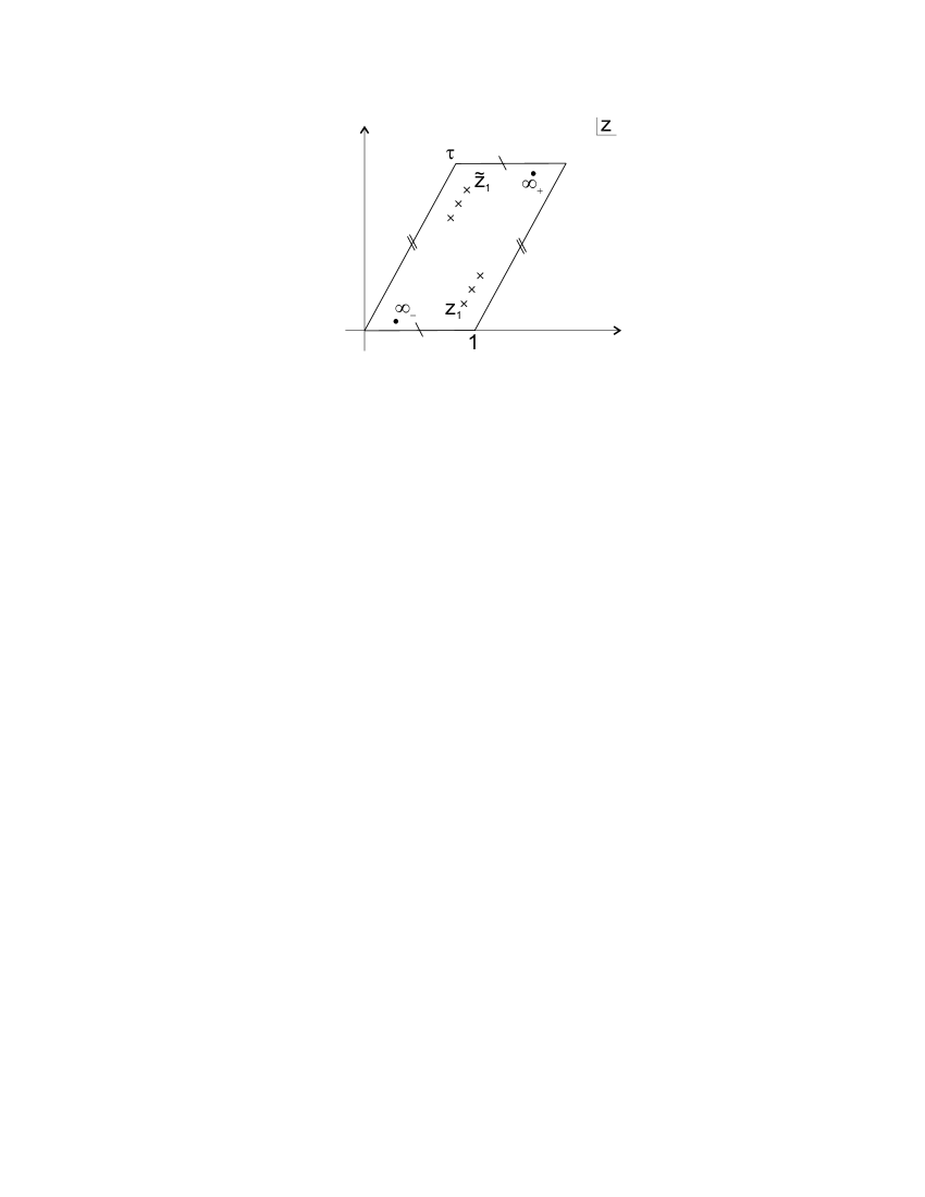
Figure 2: The figure shows the torus with modular parameter $\tau$ and the two points $\infty_{+}$ and $\infty_{-}$ corresponding to the infinities, denoted by dots, on the upper and lower sheet. Also shown are the points $z_{i}$, denoted by crosses, corresponding to the masses $m_{i}$. $\tilde{z}_{i}$ are the corresponding points on the lower sheet.

The meromorphic 1-form

Let us now construct the meromorphic 1-form with the appropriate properties. The form has to have poles at $z=\infty_{\pm}$ and $z_{i}$ such that $x(z_{i})=-m_{i}$ (see Figure 2) with the prescribed residues and integral periods:

$$\mathrm{res}_{z=\infty_{+}}\,\omega=-N_{c},\quad\mathrm{res}_{z=\infty_{-}}\,\omega=N_{c}-N_{f},\quad\mathrm{res}_{z=\tilde{z}_{i}}\,\omega=1,$$ (6.4)

$$\frac{1}{2\pi i}\int_{0}^{1}\omega=N_{1},\quad\frac{1}{2\pi i}\int_{0}^{\tau}\omega=\Delta k\ ,$$ (6.5)

where we have used that the $\alpha$-cycle integration corresponds to integrating from $0$ to $1$ on the torus, and the $\beta$-cycle from $0$ to $\tau$. We again have to think of definite curves for the integration not encircling the poles of $\omega$.

On the torus we have unique one-forms $\omega_{PQ}$ which have zero $\alpha$ period and simple poles in $P$ and $Q$ with residues $+1$ and $-1$ respectively. Using these we can write $\omega$ uniquely:

$$\omega=N_{c}\omega_{\infty_{-}\infty_{+}}+\sum_{i}\omega_{\tilde{z}_{i}\infty_{-}}+2\pi iN_{1}\mathrm{d}z\ ,$$ (6.6)

where we have used that after determining the residues the only redundancy is in the addition of a holomorphic one-form which on the torus has the simple form of a constant times $\mathrm{d}z$. The constant is then determined by the $\alpha$-period in (6.5). The remaining $\beta$-period gives a constraint determining $\infty_{+}$ (which is equal to $-\infty_{-}$ modulo $(1,\tau)$). Thus it seems like no continuous parameter is undetermined on the torus except the modular parameter $\tau$. However, for the embedding we have a scalar factor and a translation. We will see that we determine the scale factor using (4.6) thus leaving us with two continuous parameters.

Now, the main point is that on the torus we have a formula for $\omega_{PQ}$ using the elliptic theta function:

$$\theta(z,\tau)=\sum_{n=-\infty}^{\infty}e^{i\pi\tau n^{2}+i2\pi zn}\ .$$ (6.7)

We will often suppress the $\tau$ dependence and just write $\theta(z)$. The theta function is a multiplicative holomorphic function with periods

$$\theta(z+1,\tau)=\theta(z,\tau),\quad\theta(z+\tau,\tau)=e^{-i\pi\tau-i2\pi z}\theta(z,\tau)\ .$$ (6.8)

Importantly, $\theta(z)$ is only zero in $(1+\tau)/2$ and the multiplicity is one. Using (6.8) this gives us the formula for $\omega_{PQ}$ (see e.g. [43])

$$\omega_{PQ}=\mathrm{d}\log\frac{\theta(z-P+\tfrac{1+\tau}{2})}{\theta(z-Q+\tfrac{1+\tau}{2})}=\frac{\theta^{\prime}(z-P+\tfrac{1+\tau}{2})}{\theta(z-P+\tfrac{1+\tau}{2})}\mathrm{d}z-\frac{\theta^{\prime}(z-Q+\tfrac{1+\tau}{2})}{\theta(z-Q+\tfrac{1+\tau}{2})}\mathrm{d}z\ .$$ (6.9)

Using (6.6) we thus get an explicit expression for $\omega$:

$$\omega=N_{c}\mathrm{d}\log\frac{\theta(z-\infty_{-}+\tfrac{1+\tau}{2})}{\theta(z-\infty_{+}+\tfrac{1+\tau}{2})}+\sum_{i}\mathrm{d}\log\frac{\theta(z-\tilde{z}_{i}+\tfrac{1+\tau}{2})}{\theta(z-\infty_{-}+\tfrac{1+\tau}{2})}+2\pi iN_{1}\mathrm{d}z\ .$$ (6.10)

We should now perform the $\beta$-cycle integration in (6.5). Using (6.8) this gives

$$-N_{c}\infty_{+}+(N_{c}-N_{f})\infty_{-}+\sum_{i}\tilde{z}_{i}+N_{1}\tau=\Delta k\ ,$$ (6.11)

which also directly follows from $\int_{\beta}\omega_{PQ}=2\pi i(P-Q)$. We may now use the relation (6.3) between $\infty_{+}$ and $\infty_{-}$ derived earlier to obtain

$$\infty_{-}=\frac{(N_{1}-N_{c})\tau-\Delta k-N_{c}+\sum_{i}\tilde{z}_{i}}{N_{f}-2N_{c}}\ ,$$ (6.12)

where we think modulo $(1,\tau)$ on the torus. Note that, as is suggested by this equation, we could trade in $N_{1}$ and $\Delta k$ for the location of the flavor poles in appropriate copies of the fundamental domain.

At this stage we have uniquely fixed the meromorphic 1-form $\omega$ and hence we may now extract the factorization solution.

Factorization solution

The $u_{k}$’s are given by calculating the residues of $x(z)^{k}\omega$ at $z=\infty_{+}$ using (4.2):

$$u_{k}^{({\rm fact})}=-\frac{1}{k}\mathrm{res}_{z=\infty_{+}}\,x^{k}\omega\ .$$ (6.13)

We thus have to construct the embedding map $x(z)$. It has to be a meromorphic map with single poles at $\infty_{+}$, $\infty_{-}$. Then necessarily it will have two zeroes $z_{0}$ and, since it should be invariant under the $\mathbb{Z}_{2}$ map, $\tilde{z}_{0}=1+\tau-z_{0}$. It is thus fixed uniquely up to a multiplicative constant $B$ and the embedding map takes the form

$$x(z)=B\frac{\theta(z-z_{0}+\tfrac{1+\tau}{2})\theta(z-1-\tau+z_{0}+\tfrac{1+\tau}{2})}{\theta(z-\infty_{+}+\tfrac{1+\tau}{2})\theta(z-\infty_{-}+\tfrac{1+\tau}{2})}\ ,$$ (6.14)

In order to compute the complete solutions it remains to determine $\Lambda$. To this end let us perform the integral in (4.6): We take $z_{\Lambda_{0}}$ as the point corresponding to $\Lambda_{0}$ on the upper sheet, i.e. we think of $z_{\Lambda_{0}}$ as being close to $\infty_{+}$. Then $\widetilde{z_{\Lambda_{0}}}=1+\tau-z_{\Lambda_{0}}$. Using (6.10) we get

$$\int_{1+\tau-z_{\Lambda_{0}}}^{z_{\Lambda_{0}}}\omega=-\log(z_{\Lambda_{0}}-\infty_{+})^{2N_{c}-N_{f}}+\log\theta(\infty_{+}-\infty_{-}+\tfrac{1+\tau}{2})^{2N_{c}-N_{f}}\\ +\sum_{i}\log\frac{\theta(\infty_{+}-\tilde{z}_{i}+\tfrac{1+\tau}{2})}{\theta(\infty_{-}-\tilde{z}_{i}+\tfrac{1+\tau}{2})}+\log\theta^{\prime}(\tfrac{1+\tau}{2})^{N_{f}-2N_{c}}\\ +(N_{c}+N_{1})2\pi i(\infty_{+}-\infty_{-})-N_{f}\pi i+\mathcal{O}(z_{\Lambda_{0}}-\infty_{+})\ ,$$ (6.15)

where we have used $\theta(-z+\tfrac{1+\tau}{2})=\exp(i\pi+i2\pi z)\theta(z+\tfrac{1+\tau}{2})$ which can be proven using (6.8) and that $\theta(z)$ is an even function. Since $x(z)$ has a pole of order one at $\infty_{+}$ we can write

$$\Lambda_{0}=x(z_{\Lambda_{0}})=A\frac{1}{z_{\Lambda_{0}}-\infty_{+}}+\mathcal{O}((z_{\Lambda_{0}}-\infty_{+})^{0})\ ,$$ (6.16)

where $A$ is a constant. Thus

$$\Lambda_{0}(z_{\Lambda_{0}}-\infty_{+})=A+\mathcal{O}(z_{\Lambda_{0}}-\infty_{+})\ .$$ (6.17)

Hence we get the relation

$$\log\Lambda_{0}^{2N_{c}-N_{f}}+\log(z_{\Lambda_{0}}-\infty_{+})^{2N_{c}-N_{f}}=\log A^{2N_{c}-N_{f}}+\mathcal{O}(z_{\Lambda_{0}}-\infty_{+})\ .$$ (6.18)

Using this to equate (4.6) and (6.15), we finally see that (4.6) determines the scale $A$ of $x(z)$:

$$\log A^{2N_{c}-N_{f}}=\log\Lambda^{2N_{c}-N_{f}}+\log\theta(\infty_{+}-\infty_{-}+\tfrac{1+\tau}{2})^{2N_{c}-N_{f}}\\ +\sum_{i}\log\frac{\theta(\infty_{+}-\tilde{z}_{i}+\tfrac{1+\tau}{2})}{\theta(\infty_{-}-\tilde{z}_{i}+\tfrac{1+\tau}{2})}+\log\theta^{\prime}(\tfrac{1+\tau}{2})^{-2N_{c}+N_{f}}\\ +(N_{c}+N_{1})2\pi i(\infty_{+}-\infty_{-})-N_{f}\pi i\ .$$ (6.19)

This is solved as

$$A=\Lambda e^{\frac{i2\pi k}{2N_{c}-N_{f}}}\frac{\theta(\infty_{+}-\infty_{-}+\tfrac{1+\tau}{2})}{\theta^{\prime}(\tfrac{1+\tau}{2})}\Big{(}\prod_{i}\frac{\theta(\infty_{+}-\tilde{z}_{i}+\tfrac{1+\tau}{2})}{\theta(\infty_{-}-\tilde{z}_{i}+\tfrac{1+\tau}{2})}\Big{)}^{\frac{1}{2N_{c}-N_{f}}}\\ \times e^{2\pi i(\infty_{+}-\infty_{-})\frac{N_{c}+N_{1}}{2N_{c}-N_{f}}}e^{-\pi i\frac{N_{f}}{2N_{c}-N_{f}}}\ ,$$ (6.20)

where $k$ is an integer, $k=0,\ldots,2N_{c}-N_{f}-1$, which is a discrete parameter of our solution.

Let us now relate $A$ to the scalar factor $B$ appearing in the expression (6.14) for the embedding $x(z)$ using $\lim_{z\rightarrow\infty_{+}}x(z)(z-\infty_{+})=A$. The resulting expression for $B$ is

$$B=\Lambda e^{\frac{i2\pi k}{2N_{c}-N_{f}}}\frac{\theta(\infty_{+}-\infty_{-}+\tfrac{1+\tau}{2})^{2}}{\theta(\infty_{+}-z_{0}+\tfrac{1+\tau}{2})\theta(\infty_{+}-1-\tau+z_{0}+\tfrac{1+\tau}{2})}\\ \times\Big{(}\prod_{i}\frac{\theta(\infty_{+}-\tilde{z}_{i}+\tfrac{1+\tau}{2})}{\theta(\infty_{-}-\tilde{z}_{i}+\tfrac{1+\tau}{2})}\Big{)}^{\frac{1}{2N_{c}-N_{f}}}e^{2\pi i(\infty_{+}-\infty_{-})\frac{N_{c}+N_{1}}{2N_{c}-N_{f}}}e^{-\pi i\frac{N_{f}}{2N_{c}-N_{f}}}\ .$$ (6.21)

Thus we have solved the problem and the solution is summarized by Eqs. (6.10), (6.13), (6.14) and (6.21). As expected, the construction depends on the two continuous parameters $\tau$ and $z_{0}$ (modulo $(1,\tau)$) and the discrete parameters $N_{1},\Delta k$ and $k$. The physical given parameters are $N_{c},N_{f},\Lambda$ and the masses $m_{i}$. In principle we should determine the $\tilde{z}_{i}$s, $i=1,\ldots,N_{f}$, using

$$x(\tilde{z}_{i})=-m_{i},\quad i=1,\ldots,N_{f}\ .$$ (6.22)

However, the dependence on $\tilde{z}_{i}$ is extremely complicated since also $x(z)$ in (6.14) depends on the $\tilde{z}_{i}$s through $B$ (see (6.21)). There is, however, one exception: If all the masses are the same, $m_{i}=m$, and correspondingly $\tilde{z}_{i}=\tilde{z}_{1}$. Then we can consider $x^{\prime}(z)=x(z)+m$. This is zero in $\tilde{z}_{1}$ and has the same poles as $x$. Thus $x^{\prime}$ is given by (6.14) and (6.21) with $\tilde{z}_{1}=z_{0}$, and (6.13) is replaced by

$$u_{k}^{({\rm fact})}=-\frac{1}{k}\mathrm{res}_{z=\infty_{+}}\,(x^{\prime}-m)^{k}\omega\ .$$ (6.23)

Of course, in the case of different masses we can in the same way trade $z_{0}$ for an arbitrary $\tilde{z}_{i}$ leaving only $N_{f}-1$ points to be determined by (6.22).

As a consistency check of our solution we have also considered the decoupling of (infinitely) massive flavors and checked that our formulas reduce to the case of pure ${\cal N}=2$ theory without flavors. We present some details of the computation in Appendix B.

We note that the solution satisfies a multiplication map. This map was found in Ref. [3, 19] for the case without flavors and further generalized to the case with flavors in Ref. [33]. For any solution, with given $N_{c}$, $N_{1}$, $\Delta k$, it follows from (6.11), (6.12), (6.21) that we also have a solution for $tN_{c}$, $tN_{1}$, $t\Delta k$ with $t$ an integer, while at the same time each $\tilde{z}_{i}$ is mapped onto $t$ copies of the same $\tilde{z}_{i}$.

We finally remark that not all of the above discrete and continuous parameters in the set $(N_{1},\Delta k,k,\tau,z_{0})$ give rise to different solutions. E.g. the periodicity in $k$ is manifest and hence we have

$$(N_{1},\Delta k,k)\equiv(N_{1},\Delta k,k+2N_{c}-N_{f})\ .$$ (6.24)

Also the periodicities of $N_{1}$ and $\Delta k$ can be found

$$(N_{1},\Delta k-(N_{f}-2N_{c}),k)\equiv(N_{1},\Delta k,k-2N_{c}-2N_{1})\ ,$$ (6.25)

$$(N_{1}+N_{f}-2N_{c},\Delta k,k)\equiv(N_{1},\Delta k,k-2\Delta k)\ .$$ (6.26)

Equation (6.25) is easily seen noting that $\infty_{-}$ from Eq. (6.12) changes by one. However, this do not change the theta functions in the formula for $x$. Thus the relation follows directly from Eq. (6.21). On the other hand, the periodicity in $N_{1}$ changes $\infty_{-}$ by $\tau$ and this means that $x$ and the scale $B$ changes non-trivially and the relation requires a calculation to check.

Similarly, we also expect modular transformations that change $\tau$ to $\tau+1$ or $-1/\tau$. This structure of the ${\cal N}=1$ vacua will be the subject of future investigation.

7 Conclusions

In this paper we have constructed an explicit solution of the factorization problem of SW-curves for ${\cal{N}}=2$ supersymmetric $U(N_{c})$ gauge theory with $N_{f}$ fundamental flavors, when the gauge symmetry is broken according to $U(N_{c})\rightarrow U(N_{1})\times U(N_{2})$. As a by-product we have rederived in a simpler way the genus zero case of complete factorization first obtained in Ref. [24]. Furthermore, for $N_{f}=0$ we get a closed formula for the genus one case which was first solved in Ref. [22]. We have also proven a theorem that holds for the general factorization. Finally, we have seen that our results can be applied to examine for what different sets of parameters one obtains the same factorized SW-curve, and hence the same physics. This is of relevance for the structure of ${\cal{N}}=1$ vacua.

There are a number of interesting open issues that would be worth studying. First of all, one could generalize the construction, including the one without flavors, to other classical gauge groups. Furthermore, it is still an open problem, also in the case with no flavors present, to find a similar explicit solution for the case of higher genus. Another direction would be to consider the more complicated case of quiver gauge theories where nonhyperelliptic curves appear [44]. It would also be interesting to apply the results here more directly to the Dijkgraaf-Vafa proposal as was done for the exact results in the one-cut case in Ref. [5].

Finally, we note that the existence of an exact solution is most interesting from the point of view of studying in detail the global structure of ${\cal{N}}=1$ vacua following Ref. [19, 32]. The features that were found there, including connected components of vacua and possible dual descriptions of the same physics, are intimately related to the discrete identifications between the parameters that label the factorization solution. In this connection, it would be interesting to see if our results can be used to further examine the phase structure using the recent work of Ref. [45]. Here a fascinating connection was found between factorization of SW-curves and Grothendieck’s “dessins d’enfants”. More generally, a relation was conjectured between the programme of classifying these dessins into Galois orbits and the problem of classifying special phases of ${\cal{N}}=1$ vacua.

Acknowledgments. We would like to thank Min-xin Huang for discussion.

RJ was supported in part by Polish Ministry of Science and Information Society Technologies grants 2P03B08225 (2003-2006), 1P03B02427 (2004-2007) and 1P03B04029 (2005-2008). Work partially supported by the European Community’s Human Potential Programme under contracts MRTN-CT-2004-005616, ‘European Network on Random Geometry’ and MRTN-CT-2004-005104, ‘Constituents, fundamental forces and symmetries of the universe’.

Appendix A Factorization and Existence of the Meromorphic One-Form

In this appendix we will prove that the SW-curve with fundamental matter factorizes as in (3.1) if and only if there exist a meromorphic one-form with only simple poles on a hyperelliptic curve, $y_{\rm red}^{2}=F_{2(N_{c}-n)}(x)$, which has residue $-N_{c}$ at infinity on the upper sheet, residue $N_{c}-N_{f}$ at infinity on the lower sheet, residue $1$ at $-m_{i}$, fulfills (4.6), and, finally, has integral $\alpha$- and $\beta$-periods. Note that $N_{c}$, $N_{f}$, $m_{i}$ and $\Lambda$ are thought of as given.

This was proven in the case without fundamental matter in [22]. The ideas here are much the same. The proof is independent of the genus and is thus not confined to the genus one curves considered above.

Let us first, for completeness, consider the easy part of the proof and show that factorization of the SW-curve implies the existence of the meromorphic 1-form on the reduced curve with the prescribed properties.

Factorization implies integral 1-form

In the first part of the proof we consider the factorized SW-curve (3.1) as given. Let us define

$$\omega\equiv\bigg{(}\frac{P^{\prime}_{N_{c}}(x)}{y(x)}+\frac{B^{\prime}(x)}{2B(x)}-\frac{P_{N_{c}}(x)B^{\prime}(x)}{2y(x)B(x)}\bigg{)}\mathrm{d}x\ .$$ (A.1)

This is nicely a meromorphic one-form on the SW-curve (2.6):

$$y^{2}=P_{N_{c}}(x)^{2}-4\Lambda^{2N_{c}-N_{f}}B(x)\ ,$$ (A.2)

where $B(x)=\prod_{i=1}^{N_{f}}(x+m_{i})$. In fact, using (A.2) we get (4.5):

$$\omega=\mathrm{d}\log(P_{N_{c}}(x)+y(x))\ ,$$ (A.3)

which tells us that $\omega$ has integral periods. From (A.1) we can also see that $\omega$ has the right poles and residues. However, since the curve is now factorized according to  (3.1):

$$y^{2}=P_{N_{c}}(x)^{2}-4\Lambda^{2N_{c}-N_{f}}B(x)=F_{2(N_{c}-n)}(x)H_{n}(x)^{2}=y_{\rm red}^{2}H_{n}(x)^{2}\ ,$$ (A.4)

we should check that we do not have poles at the zeroes of $H_{n}$. Therefore let $x_{0}$ be a root in $H_{n}$. Then by (A.4) $x_{0}$ is a double root in $y^{2}$ and hence a root in both $y^{2}$ and $dy^{2}/dx$. This gives

$$P_{N_{c}}(x_{0})^{2}-4\Lambda^{2N_{c}-N_{f}}B(x_{0})=0\ ,$$ (A.5)

$$2P_{N_{c}}(x_{0})P^{\prime}_{N_{c}}(x_{0})-4\Lambda^{2N_{c}-N_{f}}B^{\prime}(x_{0})=0\ .$$ (A.6)

We will assume $B(x_{0})\neq 0$ and hence $P_{N_{c}}(x_{0})\neq 0$. Thus we get from (A.5) and (A.6)

$$P^{\prime}_{N_{c}}(x_{0})-\frac{1}{2}P_{N_{c}}(x_{0})\frac{B^{\prime}(x_{0})}{B(x_{0})}=0\ .$$ (A.7)

Thus rewriting $\omega$ from (A.1) as

$$\omega=\bigg{(}\frac{P^{\prime}_{N_{c}}(x)-\frac{1}{2}P_{N_{c}}(x)\frac{B^{\prime}(x)}{B(x)}}{H_{n}(x)}\frac{1}{y_{\rm red}(x)}+\frac{B^{\prime}(x)}{2B(x)}\bigg{)}\mathrm{d}x\ ,$$ (A.8)

we see by (A.7) that the zeroes of $H_{n}$ are cancelled and we do not get any poles from $H_{n}$. Thus we have proven that we have a meromorphic one-form on the reduced curve, $y_{\rm red}$, with the right poles and residues and with integral periods. That $\omega$ fulfills (4.6) follows directly from (A.3) given that $P_{N_{c}}$ is normalized.

Before going to the second part of the proof let us get a little inspiration from this case where we assume that the SW-curve factorizes. In the following if $x$ is a point in the upper sheet then (with obvious abuse of notation) $\tilde{x}$ is the corresponding point on the lower sheet. By (A.1) we then get (since $y(\tilde{x})=-y(x)$):

$$\omega(x)+\omega(\tilde{x})=\frac{B^{\prime}}{B}\ .$$ (A.9)

Now, let $a$ denote a branch point of $y_{\rm red}$. Then integrating (A.3) gives

$$P_{N_{c}}(a)e^{\int_{a}^{x}\omega}=P_{N_{c}}(x)+y(x)\ ,$$ (A.10)

$$P_{N_{c}}(a)e^{\int_{a}^{\tilde{x}}\omega}=P_{N_{c}}(x)-y(x)\ .$$ (A.11)

Performing the integrations entirely on the upper/lower sheet we get from (A.9):

$$\int_{a}^{\tilde{x}}\omega=-\int_{a}^{x}\omega+\log\frac{B(x)}{B(a)}\ .$$ (A.12)

Using this and choosing $P_{N_{c}}(a)=2\Lambda^{\frac{2N_{c}-N_{f}}{2}}\sqrt{B(a)}$ we find by addition of (A.10) and (A.11) that

$$P_{N_{c}}(x)=2\Lambda^{\frac{2N_{c}-N_{f}}{2}}\sqrt{B(a)}\left(\frac{1}{2}e^{\int_{a}^{x}\omega}+\frac{1}{2}\frac{B(x)}{B(a)}e^{-\int_{a}^{x}\omega}\right)\ .$$ (A.13)

This is independent of the chosen path of integration since $\omega$ has integral periods. (A.13) is the generalization for the formula for the case without fundamental matter found in [22]. There the generalization of the Chebyshev polynomials from the one-cut case was found to be $P(x)\propto\cosh(\int_{a}^{x}\omega)$ which we get from (A.13) by taking $B(x)$ to be constant.

Let us now use the above considerations to complete the proof of the theorem.

Integral 1-form on the reduced curve implies factorization

For the second part of the proof we take as given a hyperelliptic curve $y_{\rm red}$ and a meromorphic one-form $\omega$ on $y_{\rm red}$ with the prescribed poles, residues, integral periods, and fulfilling (4.6). In this case we simply define ($a$ is again a branch point and we will, as above, assume that $B$ and $y_{\rm red}^{2}$ do not share roots)

$$P_{N_{c}}(x)\equiv 2\Lambda^{\frac{2N_{c}-N_{f}}{2}}\sqrt{B(a)}\left(\frac{1}{2}e^{\int_{a}^{x}\omega}+\frac{1}{2}\frac{B(x)}{B(a)}e^{-\int_{a}^{x}\omega}\right)\ ,$$ (A.14)

where we of course do not know if this is a polynomial. However, we do know $P_{N_{c}}$ is well-defined in the sense that it is independent of the choice of integration since $\omega$ has integral periods. To show that $P_{N_{c}}$ is indeed polynomial we will first have to see that $\omega$ fulfills (A.9). We know that we can express $\omega$ in the unique meromorphic one-forms $\omega_{PQ}$ with simple poles in $P$ and $Q$ with residues $+1$ and $-1$, respectively, and zero $\alpha$-periods. In this way we can write

$$\omega=-N_{c}\omega_{\infty_{+}\infty_{-}}+\sum_{i}\omega_{\widetilde{-m_{i}}\infty_{-}}+\textrm{holo. one-forms}\ ,$$ (A.15)

as in (6.6) but where we now have a general genus and the points are on the two sheets, not on the (generalized) torus. We can now use that

$$\omega_{\infty_{+}\infty_{-}}(x) = -\frac{x^{g}}{y_{\rm red}(x)}\mathrm{d}x+\textrm{holo. one-forms}\ ,$$ (A.16)

$$\omega_{\tilde{P}\infty_{-}}(x) = \frac{1}{2}\frac{1}{x-P}\mathrm{d}x-\frac{1}{2}\frac{1}{x-P}\frac{x^{g+1}}{y_{\rm red}(x)}\frac{y_{\rm red}(P)}{P^{g+1}}\mathrm{d}x$$

$$-\frac{1}{2}\left(1-\frac{y(P)}{P^{g+1}}\right)\frac{x^{g}}{y_{\rm red}(x)}\mathrm{d}x+\textrm{holo. one-forms}\ .$$

Here $g$ is the genus of the reduced curve, i.e. if $y_{\rm red}^{2}=F_{2(N_{c}-n)}(x)$ then $g=N_{c}-n-1$. Further a basis for the holomorphic one-forms takes the form

$$\frac{x^{i}}{y_{\rm red}(x)}\mathrm{d}x,\quad i=0,\ldots,g-1\ .$$ (A.18)

Thus we can write $\omega$ in (A.15) as

$$\omega(x)=\frac{1}{y_{\rm red}(x)}\left(R_{g}(x)-\frac{1}{2}\sum_{i}\frac{x^{g+1}}{x+m_{i}}\frac{y_{\rm red}(-m_{i})}{(-m_{i})^{g+1}}\right)\mathrm{d}x+\frac{1}{2}\sum_{i}\frac{1}{x+m_{i}}\mathrm{d}x\ ,$$ (A.19)

where $R_{g}(x)$ is some polynomial of degree $g$ and we recognize the last term as the expression $\tfrac{1}{2}B^{\prime}(x)/B(x)\mathrm{d}x$. From this (A.9) is immediate. (A.9) then tells us that $P_{N_{c}}$ is continuous across the cuts (it is of course by definition continuous through the cuts) since using (A.12):

$$P_{N_{c}}(\tilde{x}) = 2\Lambda^{\frac{2N_{c}-N_{f}}{2}}\sqrt{B(a)}\left(\frac{1}{2}e^{-\int_{a}^{x}\omega+\log\frac{B(x)}{B(a)}}+\frac{1}{2}\frac{B(x)}{B(a)}e^{\int_{a}^{x}\omega-\log\frac{B(x)}{B(a)}}\right)$$ (A.20)

$$= P_{N_{c}}(x)\ .$$

This means that $P_{N_{c}}$ can be continued to a holomorphic function in the (non-compact) complex plane with the possible exception of the poles of $\omega$ i.e. $\widetilde{-m_{i}}$. However, the value of $P_{N_{c}}$ here is the same value as in $-m_{i}$ by (A.20) and the are no poles in $-m_{i}$ at the upper sheet. Thus we only have to care about the behavior of $P_{N_{c}}$ at infinity. Since $\int_{a}^{x}\omega\sim N_{c}\log x$ for $x$ going to infinity we get

$$\log P_{N_{c}}(x)\sim\log\big{(}e^{N_{c}\log x}+\frac{x^{N_{f}}}{B(a)}e^{-N_{c}\log x}\big{)}=\log\big{(}x^{N_{c}}+\frac{x^{N_{f}-N_{c}}}{B(a)}\big{)}\sim N_{c}\log x\ ,$$ (A.21)

since $N_{f}\leq 2N_{c}$. We can thus conclude that $P_{N_{c}}(x)$ is a polynomial of degree $N_{c}$ as wanted. That $P_{N_{c}}$ is correctly normalized follows by redoing the calculation in (A.21) also including the $x^{0}$-order and this time using the assumption (4.6) and the derived equation (A.12).

Having established that $P_{N_{c}}$ is a polynomial it follows that

$$y^{2}\equiv P_{N_{c}}(x)^{2}-4\Lambda^{2N_{c}-N_{f}}B(x)\ ,$$ (A.22)

must also be polynomial. Now, all we need to prove is that $y^{2}=y_{\rm red}^{2}H_{n}(x)^{2}$ for some polynomial $H_{n}$. Using equation (A.14) we get

$$y^{2}=4\Lambda^{2N_{c}-N_{f}}B(a)\left(\frac{1}{4}e^{2\int_{a}^{x}\omega}+\frac{1}{4}\frac{B(x)^{2}}{B(a)^{2}}e^{-2\int_{a}^{x}\omega}-\frac{1}{2}\frac{B(x)}{B(a)}\right)\ .$$ (A.23)

To see that $y^{2}$ contains $y_{\rm red}^{2}$ as a factor we first realize that $a$, which was a root in $y_{\rm red}$, is also trivially a root in $y^{2}$ by inserting $a$ in (A.23). Let now $b$ be any other root in $y_{\rm red}^{2}$. We want to know the value of $\exp(\pm 2\int_{a}^{b}\omega)$. To find these values we first note that the $\alpha$- and $\beta$-cycles on $y_{\rm red}$ can all be seen as curves from one branch point to another on the upper sheet and then back again (i.e. in the reverse direction) on the lower sheet (think of continuous deformations of the curves in Figure 1). The curve in the integral $\int_{a}^{b}\omega$ can then be seen as being put together of the upper sheet parts of the $\alpha$- and $\beta$-curves. We can then write (using (A.12) and explicitly writing whether the integral is taken on the upper or the lower sheet):

$$\int_{a}^{b}\omega\Big{\lvert}_{upper} = \frac{1}{2}\int_{a}^{b}\omega\Big{\lvert}_{upper}-\frac{1}{2}\int_{a}^{b}\omega\Big{\lvert}_{lower}+\frac{1}{2}\log\frac{B(b)}{B(a)}$$ (A.24)

$$= \frac{1}{2}\int_{\sum_{i}c_{i}\alpha_{i}+c^{\prime}_{i}\beta_{i}}\omega+\frac{1}{2}\log\frac{B(b)}{B(a)}\ ,$$

where the first integral in the last line simply is the half of a sum of $\alpha$- and $\beta$-periods of $\omega$ ($c_{i}$ and $c^{\prime}_{i}$ are $\pm 1$ or zero). However, since we know that the periods are integral (this is the crucial dependence on the integrality of the periods) the first integral in the last line simply is an integer times $i\pi$. Thus inserting in (A.23) gives

$$y^{2}(b)=4\Lambda^{2N_{c}-N_{f}}B(a)\left(\frac{1}{4}\frac{B(b)}{B(a)}+\frac{1}{4}\frac{B(b)}{B(a)}-\frac{1}{2}\frac{B(b)}{B(a)}\right)=0\ .$$ (A.25)

Thus the integrality of $\omega$ gives us that $y^{2}$ contains $y_{\rm red}^{2}$ as a factor, so that

$$y^{2}(x)=y_{\rm red}^{2}(x)Q(x)\ .$$ (A.26)

To complete the proof we simply have to show that $Q(x)$ is the square of a polynomial. First we note that

$$y(x)=2\Lambda^{\frac{2N_{c}-N_{f}}{2}}\sqrt{B(a)}\left(\frac{1}{2}e^{\int_{a}^{x}\omega}-\frac{1}{2}\frac{B(x)}{B(a)}e^{-\int_{a}^{x}\omega}\right)\ ,$$ (A.27)

since this nicely fulfills (A.23) (we ignore the sign choice). We can then calculate

$$\frac{1}{\sqrt{Q}}\frac{dy^{2}}{dx}=\frac{y_{\rm red}}{y}\frac{dy^{2}}{dx}=\frac{y_{\rm red}}{y}\left(2P_{N_{c}}P^{\prime}_{N_{c}}-4\Lambda^{2N_{c}-N_{f}}B^{\prime}\right)\\ \stackrel{{\scriptstyle\eqref{appeqn12},\eqref{appeqn24}}}{{=}}\frac{y_{\rm red}}{y}\left(2P_{N_{c}}\left(y\frac{\omega}{\mathrm{d}x}+2\Lambda^{\frac{2N_{c}-N_{f}}{2}}\sqrt{B(a)}\frac{1}{2}\frac{B^{\prime}}{B(a)}e^{-\int_{a}^{x}\omega}\right)-4\Lambda^{2N_{c}-N_{f}}B^{\prime}\right)\\ \stackrel{{\scriptstyle\eqref{appeqn12},\eqref{appeqn24}}}{{=}}\frac{y_{\rm red}}{y}\left(2P_{N_{c}}\left(y\frac{\omega}{\mathrm{d}x}+\frac{1}{2}\frac{B^{\prime}}{B}(P-y)\right)-4\Lambda^{2N_{c}-N_{f}}B^{\prime}\right)\\ \stackrel{{\scriptstyle\eqref{appeqn16.5},\eqref{appeqn19}}}{{=}}\frac{y_{\rm red}}{y}\left(2P_{N_{c}}y\frac{1}{y_{\rm red}}\left(R_{g}-\frac{1}{2}\sum_{i}\frac{x^{g+1}}{x+m_{i}}\frac{y_{\rm red}(-m_{i})}{(-m_{i})^{g+1}}\right)+y^{2}\frac{B^{\prime}}{B}\right)\\ \stackrel{{\scriptstyle\eqref{appeqn23}}}{{=}}\tilde{R}+y^{2}_{red}\sqrt{Q}\frac{B^{\prime}}{B}\ ,$$ (A.28)

where $\tilde{R}$ is some rational function. Solving this for $\sqrt{Q}$ gives

$$\sqrt{Q(x)}=\frac{1}{\tilde{R}(x)}\left(\frac{dy^{2}}{dx}-y^{2}_{red}\frac{B^{\prime}}{B}Q\right)\ .$$ (A.29)

Since $\sqrt{Q}$ is the square-root of a polynomial and the right hand side is a rational function we can finally conclude that $\sqrt{Q}$ is a polynomial, thus finishing the proof.

The given one-form $\omega$ must then – by uniqueness given the $\alpha$-periods – be $T(x)\mathrm{d}x$ from equation (4.1) and thus (4.2) applies.

Appendix B Flavor decoupling

We can obtain the case without fundamental flavors by taking the limits described after equation (2.7). This means that we should take $\Lambda\rightarrow 0$ and $m_{i}\rightarrow\infty$ for all $i$ while keeping constant:

$$\Lambda^{2N_{c}-N_{f}}\prod_{i}m_{i}\equiv\Lambda_{\rm new}^{2N_{c}}\ ,$$ (B.1)

where $\Lambda_{\rm new}$ is the new scale for the theory without flavors. The limit means that for all $i$ we have $\tilde{z}_{i}\rightarrow\infty_{-}$. However, $\infty_{-}$ is itself changed by changing the $\tilde{z}_{i}$s so from (6.12) we get the consistency equation

$$\infty_{-}=\frac{(N_{1}-N_{c})\tau-\Delta k-N_{c}+N_{f}\infty_{-}}{N_{f}-2N_{c}}\ ,$$ (B.2)

which, as could be expected, is solved as

$$\infty_{-}=\frac{(N_{1}-N_{c})\tau-\Delta k-N_{c}}{-2N_{c}}\ .$$ (B.3)

For $x(z)$ in (6.14) all we should do then is to find the formula for $B$ after the limit has been taken. Using (6.14) in $m_{i}=-x(\tilde{z}_{i})$ we can rewrite equation (B.1) as

$$\lim\frac{\Lambda^{2N_{c}-N_{f}}}{\prod_{i}\theta(\tilde{z}_{i}-\infty_{-}+\tfrac{1+\tau}{2})}\bigg{(}-B\frac{\theta(\infty_{-}-z_{0}+\tfrac{1+\tau}{2})\theta(\infty_{-}-1-\tau+z_{0}+\tfrac{1+\tau}{2})}{\theta(\infty_{-}-\infty_{+}+\tfrac{1+\tau}{2})}\bigg{)}^{N_{f}}\\ =\Lambda_{\rm new}^{2N_{c}}\ .$$ (B.4)

This means we can solve for $\lim\Lambda^{2N_{c}-N_{f}}/\prod_{i}\theta(\tilde{z}_{i}-\infty_{-}+\tfrac{1+\tau}{2})$ and the result can be used in (6.21) to obtain:

$$B=e^{\frac{i2\pi k}{2N_{c}-N_{f}}}\frac{\theta(\infty_{+}-\infty_{-}+\tfrac{1+\tau}{2})^{2}}{\theta(\infty_{+}-z_{0}+\tfrac{1+\tau}{2})\theta(\infty_{+}-1-\tau+z_{0}+\tfrac{1+\tau}{2})}\\ \times\theta(\infty_{+}-\infty_{-}+\tfrac{1+\tau}{2})^{\frac{N_{f}}{2N_{c}-N_{f}}}e^{2\pi i(\infty_{+}-\infty_{-})\frac{N_{c}+N_{1}}{2N_{c}-N_{f}}}e^{-\pi i\frac{N_{f}}{2N_{c}-N_{f}}}\\ \times\Lambda_{\rm new}^{\frac{2N_{c}}{2N_{c}-N_{f}}}\bigg{(}-\frac{\theta(\infty_{-}-\infty_{+}+\tfrac{1+\tau}{2})}{B\theta(\infty_{-}-z_{0}+\tfrac{1+\tau}{2})\theta(\infty_{-}-1-\tau+z_{0}+\tfrac{1+\tau}{2})}\bigg{)}^{\frac{N_{f}}{2N_{c}-N_{f}}}\ .$$ (B.5)

We can then solve for $B$ to obtain

$$B=\Lambda_{\rm new}e^{\frac{i2\pi k}{2N_{c}}}\frac{\theta(\infty_{+}-\infty_{-}+\tfrac{1+\tau}{2})^{2}}{\theta(\infty_{+}-z_{0}+\tfrac{1+\tau}{2})\theta(\infty_{+}-1-\tau+z_{0}+\tfrac{1+\tau}{2})}\\ \times e^{2\pi i(\infty_{+}-\infty_{-})\frac{N_{c}+N_{1}}{2N_{c}}}\ .$$ (B.6)

This gives the solution together with (6.14):

$$x(z)=B\frac{\theta(z-z_{0}+\tfrac{1+\tau}{2})\theta(z-1-\tau+z_{0}+\tfrac{1+\tau}{2})}{\theta(z-\infty_{+}+\tfrac{1+\tau}{2})\theta(z-\infty_{-}+\tfrac{1+\tau}{2})}\ ,$$ (B.7)

and the limit of (6.10):

$$\omega=N_{c}\mathrm{d}\log\frac{\theta(z-\infty_{-}+\tfrac{1+\tau}{2})}{\theta(z-\infty_{+}+\tfrac{1+\tau}{2})}+2\pi iN_{1}\mathrm{d}z\ .$$ (B.8)

This is exactly what we would get if we solved the factorization problem without fundamental matter directly.

References

- [1] N. Seiberg and E. Witten, “Electric - magnetic duality, monopole condensation, and confinement in supersymmetric Yang-Mills theory,” Nucl. Phys. B426 (1994) 19–52 [Erratum–ibid.B430:485–486,1994], hep-th/9407087.
- [2] N. Seiberg and E. Witten, “Monopoles, duality and chiral symmetry breaking in supersymmetric QCD,” Nucl. Phys. B431 (1994) 484–550, hep-th/9408099.
- [3] F. Cachazo, K. A. Intriligator, and C. Vafa, “A large duality via a geometric transition,” Nucl. Phys. B603 (2001) 3–41, hep-th/0103067.
- [4] R. Dijkgraaf and C. Vafa, “A perturbative window into non-perturbative physics,” hep-th/0208048.
- [5] F. Ferrari, “On exact superpotentials in confining vacua,” Nucl. Phys. B648 (2003) 161–173, hep-th/0210135.
- [6] R. Dijkgraaf, M. T. Grisaru, C. S. Lam, C. Vafa, and D. Zanon, “Perturbative computation of glueball superpotentials,” Phys. Lett. B573 (2003) 138–146, hep-th/0211017.
- [7] F. Cachazo, M. R. Douglas, N. Seiberg, and E. Witten, “Chiral rings and anomalies in supersymmetric gauge theory,” JHEP 12 (2002) 071, hep-th/0211170.
- [8] R. Argurio, G. Ferretti, and R. Heise, “An introduction to supersymmetric gauge theories and matrix models,” Int. J. Mod. Phys. A19 (2004) 2015–2078, hep-th/0311066.
- [9] P. B. Ronne, “On the Dijkgraaf-Vafa conjecture,” hep-th/0408103.
- [10] M. Marino, “Les Houches lectures on matrix models and topological strings,” hep-th/0410165.
- [11] K. D. Kennaway, “String theory and the vacuum structure of confining gauge theories,” hep-th/0409265.
- [12] F. Cachazo and C. Vafa, “ and geometry from fluxes,” hep-th/0206017.
- [13] R. Gopakumar, “ theories and a geometric master field,” JHEP 05 (2003) 033, hep-th/0211100.
- [14] S. G. Naculich, H. J. Schnitzer, and N. Wyllard, “The gauge theory prepotential and periods from a perturbative matrix model calculation,” Nucl. Phys. B651 (2003) 106–124, hep-th/0211123.
- [15] R. A. Janik and N. A. Obers, “ superpotential, Seiberg-Witten curves and loop equations,” Phys. Lett. B553 (2003) 309–316, hep-th/0212069.
- [16] V. Balasubramanian et al., “Multi-trace superpotentials vs. matrix models,” Commun. Math. Phys. 242 (2003) 361–392, hep-th/0212082.
- [17] R. Boels, J. de Boer, R. Duivenvoorden, and J. Wijnhout, “Factorization of Seiberg-Witten curves and compactification to three dimensions,” JHEP 03 (2004) 010, hep-th/0305189.
- [18] M. R. Douglas and S. H. Shenker, “Dynamics of supersymmetric gauge theory,” Nucl. Phys. B447 (1995) 271–296, hep-th/9503163.
- [19] F. Cachazo, N. Seiberg, and E. Witten, “Phases of supersymmetric gauge theories and matrices,” JHEP 02 (2003) 042, hep-th/0301006.
- [20] F. Ferrari, “Quantum parameter space and double scaling limits in super yang-mills theory,” Phys. Rev. D67 (2003) 085013, hep-th/0211069.
- [21] F. Ferrari, “Quantum parameter space in super Yang-Mills. II,” Phys. Lett. B557 (2003) 290–296, hep-th/0301157.
- [22] R. A. Janik, “Exact factorization of Seiberg-Witten curves and vacua,” Phys. Rev. D69 (2004) 085010, hep-th/0311093.
- [23] R. A. Janik, “Phases of theories and factorization of Seiberg-Witten curves,” Acta Phys. Pol. 36 (2005) 3837, hep-th/0510116.
- [24] Y. Demasure and R. A. Janik, “Explicit factorization of Seiberg-Witten curves with matter from random matrix models,” Nucl. Phys. B661 (2003) 153–173, hep-th/0212212.
- [25] R. Argurio, V. L. Campos, G. Ferretti, and R. Heise, “Exact superpotentials for theories with flavors via a matrix integral,” Phys. Rev. D67 (2003) 065005, hep-th/0210291.
- [26] N. Seiberg, “Adding fundamental matter to ’Chiral rings and anomalies in supersymmetric gauge theory’,” JHEP 01 (2003) 061, hep-th/0212225.
- [27] S. G. Naculich, H. J. Schnitzer, and N. Wyllard, “Matrix model approach to the gauge theory with matter in the fundamental representation,” JHEP 01 (2003) 015, hep-th/0211254.
- [28] M. Klein and S.-J. Sin, “Matrix model, Kutasov duality and factorization of Seiberg- Witten curves,” J. Korean Phys. Soc. 44 (2004) 1368–1376, hep-th/0310078.
- [29] C.-h. Ahn, B. Feng, Y. Ookouchi, and M. Shigemori, “Supersymmetric gauge theories with flavors and matrix models,” Nucl. Phys. B698 (2004) 3–52, hep-th/0405101.
- [30] M. Gomez-Reino, “Exact superpotentials, theories with flavor and confining vacua,” JHEP 06 (2004) 051, hep-th/0405242.
- [31] F. Elmetti, A. Santambrogio, and D. Zanon, “On exact superpotentials from matrix models,” JHEP 10 (2005) 104, hep-th/0506087.
- [32] F. Cachazo, N. Seiberg, and E. Witten, “Chiral rings and phases of supersymmetric gauge theories,” JHEP 04 (2003) 018, hep-th/0303207.
- [33] V. Balasubramanian, B. Feng, M.-x. Huang, and A. Naqvi, “Phases of supersymmetric gauge theories with flavors,” Annals Phys. 310 (2004) 375–427, hep-th/0303065.
- [34] C.-h. Ahn, B. Feng, and Y. Ookouchi, “Phases of gauge theories with flavors,” Phys. Rev. D69 (2004) 026006, hep-th/0307190.
- [35] C.-h. Ahn, B. Feng, and Y. Ookouchi, “Phases of gauge theories with flavors,” Nucl. Phys. B675 (2003) 3–69, hep-th/0306068.
- [36] P. Merlatti, “Gaugino condensate and phases of super Yang-Mills theories,” hep-th/0307115.
- [37] L. Alvarez-Gaume and S. F. Hassan, “Introduction to S-duality in supersymmetric gauge theories: A pedagogical review of the work of Seiberg and Witten,” Fortsch. Phys. 45 (1997) 159–236, hep-th/9701069.
- [38] P. C. Argyres, M. R. Plesser, and A. D. Shapere, “The Coulomb phase of supersymmetric QCD,” Phys. Rev. Lett. 75 (1995) 1699–1702, hep-th/9505100.
- [39] A. Hanany and Y. Oz, “On the quantum moduli space of vacua of supersymmetric gauge theories,” Nucl. Phys. B452 (1995) 283–312, hep-th/9505075.
- [40] E. D’Hoker, I. M. Krichever, and D. H. Phong, “The effective prepotential of supersymmetric gauge theories,” Nucl. Phys. B489 (1997) 179–210, hep-th/9609041.
- [41] E. D’Hoker and D. H. Phong, “Lectures on supersymmetric Yang-Mills theory and integrable systems,” hep-th/9912271.
- [42] R. A. Janik, “The Dijkgraaf-Vafa correspondence for theories with fundamental matter fields,” Acta Phys. Polon. B34 (2003) 4879–4890, hep-th/0309084.
- [43] D. Mumford, Tata lectures on theta. I. Progress in Mathematics 28, Birkhauser Boston, 1984.
- [44] R. Casero and E. Trincherini, “Phases and geometry of the quiver gauge theory and matrix models,” JHEP 09 (2003) 063, hep-th/0307054.
- [45] S. K. Ashok, F. Cachazo, and E. Dell’Aquila, “Children’s drawings from Seiberg-Witten curves,” hep-th/0611082.