Islands in the Landscape

T. Clifton, Andrei Linde and Navin Sivanandam

Department of Physics, Stanford University, Stanford, CA 94305

The string theory landscape consists of many metastable de Sitter vacua, populated by eternal inflation. Tunneling between these vacua gives rise to a dynamical system, which asymptotically settles down to an equilibrium state. We investigate the effects of sinks to anti-de Sitter space, and show how their existence can change probabilities in the landscape. Sinks can disturb the thermal occupation numbers that would otherwise exist in the landscape and may cause regions that were previously in thermal contact to be divided into separate, thermally isolated islands.

1 Introduction

One of the most intriguing features of string theory is its prediction of a multitude of vacuum states [1, 2, 3, 4, 5] Stabilizing these states [6] and coupling the resulting embarrassment of riches with a population mechanism [7, 8] provided by eternal inflation [9, 10] gives rise to the string theory landscape [11]. Physics in the landscape can be both rich and perplexing. We aim to elucidate some relevant ideas for understanding this physics, with the hope of improving our comprehension of the multiverse.

Inflationary expansion divides the universe into many exponentially large domains, each corresponding to different metastable vacuum states. In this picture tunneling between different vacuum states causes bubbles of new vacuum to be continually nucleated. Those with positive vacuum energy are initially static, but soon accelerate in their expansion until the velocity of their walls asymptotically approaches that of light. If the conditions are right inside these bubbles then a stage of slow-roll inflation will occur and the resulting observers will see themselves in an infinitely extended, open Friedmann universe. Percolation of successive bubbles inside of each other give us a universe that is eternally inflating and constantly producing new inflationary universes, where structure can form, and life can evolve.

The first step in a complete understanding of this scenario must be to find out which vacua are possible in string theory, and to describe their typical properties [3]. Once these vacua have been identified we will then need to study cosmological evolution during eternal inflation in order to determine the global structure of the universe [8]. During inflation the number of horizon-sized dS regions of space-time is continually, and exponentially, increasing. These dS regions then ‘populate’ the many possible vacua of string theory, realizing the great variety of the theory in a diverse and eternal universe.

The resulting picture is incredibly complex. Ultimately, our goal is to explain the properties of our part of the multiverse, and to predict the results of future observations. To achieve this goal one needs to calculate the probabilities of various outcomes in an eternally inflating multiverse. This is a thorny problem, and a subject of much contention. Studying the global structure of an eternally inflating spacetime leads to comparisons of infinite volumes, and hence a consequent dependence on cutoff procedures [8, 12, 13, 14, 15, 16, 17]. Escaping cutoff problems is not impossible if one considers individual observers and concentrates on their individual histories, ignoring the rest of the universe [18, 19, 20, 21, 22]; here, however, we must face the problems of initial conditions and are, perhaps, led to worry about Euclidean quantum gravity and the wave-function of the universe [23, 24, 25]. More importantly, this description tends to miss some of the important features of eternal inflation.

In this paper we will leave anthropic considerations aside and concentrate on other properties of the string theory landscape. We will focus on the existence, or otherwise, of thermal equilibrium between populations of dS vacua. As we will see, under certain conditions, a system of dS vacua described in comoving coordinates settles down to a state in which the populations of these vacua are in thermal equilibrium with one another. More precisely, the ratios of comoving volume occupied by one vacuum or another will depend on the exponential of the entropy difference between them. An important limitation of this simple picture is that it is valid only in comoving coordinates, which do not reward different rates of cosmological expansion in different parts of the universe. Nevertheless, the picture of many dS universes in a state of thermal equilibrium is very simple and intuitively appealing, and therefore it can be very useful for understanding various features of the string theory landscape.

On the other hand, this simple picture may be invalid when the landscape has sinks (terminal vacua which can be tunneled to, but not from). In particular, in [26, 27] it was shown that for a simple system consisting of 2 dS vacua and one AdS sink, naive expectations of thermal equilibrium are incorrect if the decay rate to the sink is sufficiently fast. Since one expects sinks to be common in the landscape [26], it may be the case that the disruption of thermal equilibrium between metastable dS vacua is a generic feature, and the string theory landscape may consist of many thermally isolated ‘islands.’ The goal of this work is to elucidate this possibility and to investigate in more detail the situations in which the usual thermally equilibrium populations are disturbed. We will find explicit solutions for a variety of simple configurations that may occur in the landscape, and use these results to form a picture of how the vacua of a more realistic landscape may be populated.

It will be found that the presence of sinks in the landscape can significantly alter the dynamics of the inflating multiverse. One of the most dramatic and unexpected examples of this is that when a number of high energy vacua decay to a single lower energy vacuum, which can decay to a sink, the probability fluxes soon become dominated by the slowest decaying, most stable vacuum. In the limiting case of this vacuum being completely stable it makes no contribution at all to probability fluxes, as these are the results of tunneling events between metastable vacua (see below). However, if the smallest chance of tunneling out of this vacuum is allowed, we unexpectedly find that this tiny current comes to be the dominant source of the probability flux. This slowest decaying vacuum may then remain out of thermal contact with other vacua, whilst all faster decaying vacua eventually approach thermal equilibrium with each other. This ‘tortoise and the hare’ scenario shows explicitly the non-trivial effect of sinks on the dynamics of inflation in the string theory landscape: They may lead to the existence of thermally isolated, slowly decaying vacua while all other, more rapidly decaying vacua are left in thermal equilibrium.

We will also investigate the possibility that some of the AdS or Minkowski sinks could potentially act as impassable barriers between systems of dS vacua, thus carving the landscape into totally disconnected ‘islands’. Such a situation would result in different regions of the multiverse being completely isolated from one another, whilst maintaining thermal equilibrium internally. We argue that the large number of vacua and dimensions in the landscape, coupled with the ‘vacuum dynamics’ we find to exist in the presence of sinks, makes the existence of such isolated regions improbable, though perhaps not impossible.

In section 2 we will review the basic mechanisms of tunneling between vacua. Following this, in section 3 we will outline the results of [26, 27], for a simple landscape of two dS vacua and one AdS sink. Section 4 discusses the possibility of sinks dividing the landscape into disconnected islands. In section 5 we shall summarize the results of our investigations into more complicated toy landscapes, highlighting some of the counter-intuitive features that emerge. In section 6 we summarize our results. Mathematical details can be found in the appendix.

2 Tunneling in the Landscape

There are two related mechanisms for making transitions between vacua: one due to tunneling [28] and another due to stochastic diffusion processes [18, 29]. A somewhat more detailed discussion of these mechanisms, and the issues associated with them, can be found in [27]. We summarize the salient points below.

Tunneling between vacua produces bubbles of new vacuum, that look like infinite open Friedmann universes to observers inside. If the tunneling goes to dS space, then the bubble expands exponentially with the velocity of its walls approaching that of light. (In comoving coordinates these bubbles approach some maximal value and freeze. This maximal value depends on the time when the bubble is formed, and is exponentially smaller for bubbles formed later on [30].) If the tunneling goes to a state with a negative vacuum energy $V$, the infinite universe inside it collapses within a time of the order $|V|^{-1/2}$, in Planck units. These negative energy, AdS vacua then play the role of sinks for probability currents in the landscape.

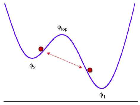
Figure 1: Coleman-De Luccia tunneling may go in both directions.

Let us consider two dS vacua, $\mathrm{dS}_{i}$, with vacuum energy density $V_{i}=V(\phi_{i})$, Fig. 1. Without taking gravity into account, the tunneling may go only from the upper minimum to the lower minimum, but in the presence of gravity tunneling may occur in both directions, which is emphasized in Fig. 1. According to Coleman and De Luccia [28], the tunneling probability from $\mathrm{dS}_{1}$ to $\mathrm{dS}_{2}$ is given by

$$\Gamma_{12}=e^{-B}=e^{-S(\phi)+S_{1}},$$ (1)

where $S(\phi)$ is the Euclidean action for the tunneling trajectory, and $S_{1}=S(\phi_{1})$ is the Euclidean action for the initial configuration $\phi=\phi_{1}$,

$$S_{1}=-{\frac{24\pi^{2}}{V_{1}}}<0\ .$$ (2)

This action has a simple sign-reversal relation to the entropy of de Sitter space, ${\bf S_{1}}$:

$${\bf S_{1}}=-S_{1}=+{24\pi^{2}\over V_{1}}\ .$$ (3)

Therefore the decay time of the metastable dS vacuum $t_{\rm decay}\sim\Gamma^{-1}_{12}$ can be represented in the following way:

$$t_{\rm decay}=e^{S(\phi)+\bf S_{1}}=t_{r}\ e^{S(\phi)}\ .$$ (4)

Here $t_{r}\sim e^{\bf S_{1}}$ is the so-called recurrence time for the vacuum $\mathrm{dS}_{1}$.

Whereas the theory of tunneling developed in [28] was quite general, all examples of tunneling studied there described the thin-wall approximation, where the tunneling occurs from one minimum of the potential and proceeds directly to another minimum. In the cases where the thin-wall approximation is not valid, the tunneling occurs not from the minimum but from the wall, which makes interpretation of this process in terms of the decay of the initial vacuum less trivial.

The situation becomes especially confusing when the potential is very flat on the way from one minimum to another, $V^{\prime\prime}<V$, in Planck units. In this case the Coleman-De Luccia (CDL) instantons describing decay of a dS space do not exist [31]; they become replaced by Hawking-Moss (HM) instantons. According to Hawking and Moss [31], the probability of tunneling from the minimum 1 to the minimum 2 is then given by

$$\Gamma_{12}=e^{-S_{\rm top}+S_{1}}=\exp\left(-{24\pi^{2}\over V(\phi_{1})}+{24\pi^{2}\over V(\phi_{\rm top})}\right)\ .$$ (5)

The HM instanton is described by the Euclidean version of dS space corresponding to the top of the potential barrier, $\phi=\phi_{\rm top}$.

Unlike the thin-wall CDL solution, the HM solution does not interpolate between the two different minima of $V(\phi)$, and therefore debates on the validity of the HM result continue even now [32]. One may wonder why we should consider such instantons instead of considering the instantons corresponding to the dS space in the next minimum; the resulting tunneling action would be much smaller. Moreover, one may consider a string theory landscape with many minima and maxima separated by a sequence of barriers. Then one could wonder whether the HM tunneling suppression applies only to the tunneling between the nearby vacua, or if it can describe direct tunneling to distant minima, ignoring all intermediate barrier except the last one [7, 32]. One of the best attempts to clarify this situation was made by Gen and Sasaki [33], who described the tunneling using Hamiltonian methods in quantum cosmology, which avoided many ambiguities of the Euclidean approach. But even their investigation does not allow us to answer the last of these questions.

A proper interpretation of the Hawking–Moss tunneling was achieved only after the development of the stochastic approach to inflation [8, 18, 29, 34]. One may consider quantum fluctuations of a light scalar field $\phi$ with $m^{2}=V^{\prime\prime}\ll H^{2}=V/3$. During each time interval $\delta t=H^{-1}$ this scalar field experiences quantum jumps with the wavelength $\sim H^{-1}$, and with a typical amplitude $\delta\phi=H/2\pi$. As a result, quantum fluctuations lead to a local change in amplitude of the field $\phi$, which looks homogeneous on the horizon scale $H^{-1}$. From the point of view of a local observer, this process looks like a Brownian motion of the homogeneous scalar field. If the potential has a dS minimum at $\phi_{1}\gg H^{2}/m$, then eventually the probability distribution to find the field with the value $\phi$ at a given point becomes (almost) time-independent,

$$P(\phi)\sim\exp\left(-{24\pi^{2}\over V(\phi_{1})}+{24\pi^{2}\over V(\phi)}\right)\ .$$ (6)

The distribution $P(\phi)$ gives the probability to find the field $\phi$ at a given point, and has a simple interpretation as the fraction of comoving volume of the universe in each of the dS vacua, or, equivalently, a fraction of time the field spends in a vicinity of its value $\phi$ along the Brownian trajectory. Up to a sub-exponential factor, this distribution shows the density of points with a given value of the field $\phi$ along its Brownian trajectory. This implies that, up to a sub-exponential factor, the typical time required for the field, at any given point in comoving coordinates, to move from its equilibrium value $\phi_{1}$ and climb to the top of the barrier is proportional to $P^{-1}(\phi_{\rm top})\sim\exp\left({24\pi^{2}\over V(\phi_{1})}-{24\pi^{2}\over V(\phi_{\rm top})}\right)$ [7]. Once the scalar field climbs to the top of the barrier, it can fall from it to the next minimum, which completes the process of “tunneling” in this regime. That is why the probability to gradually climb to the local maximum of the potential at $\phi=\phi_{\rm top}$ and then fall to another dS minimum is given by the Hawking-Moss expression (5) [18, 34, 7, 29]. It is also why tunneling to distant minima separated by many barriers is accomplished by a sequence of transitions from one minimum to another nearby minimum, rather than by one big jump. This last statement does not follow from the Hawking-Moss derivation of their result, but is apparent from the stochastic approach to inflation.

A necessary condition for the derivation of Eq. (6) using the stochastic approach to inflation in [8, 18, 29, 34] is the requirement that $m^{2}=V^{\prime\prime}\ll H^{2}=V/3$. This requirement is satisfied during slow-roll inflation, but it is violated for all known scalar fields at the present (post-inflationary) stage of the evolution of the universe. Thus the situation with the interpretation of the Coleman-De Luccia tunneling for $V^{\prime\prime}\geq V/3$ is somewhat unsatisfactory. However, since the validity of the Coleman-De Luccia approach was confirmed at least in some limiting cases (in the absence of gravity, and in the slow-roll regime discussed above), in this paper we will follow the standard lore, assume that this approach is correct, and study its consequences.

Following [35] (see also [11, 36, 38]), we will look for the probability distribution $P_{i}$ to find a given point in a state with vacuum energy $V_{i}$, and will try to generalize the results for the probability distribution obtained above by the stochastic approach to inflation. The main idea is to consider CDL tunneling between two dS vacua, with vacuum energies $V_{1}$ and $V_{2}$, such that $V_{1}<V_{2}$, and to study the possibility of tunneling in both directions, from $V_{1}$ to $V_{2}$, or vice versa.

The action on the tunneling trajectory, $S(\phi)$, does not depend on the direction in which the tunneling occurs, but the tunneling probability does depend on it. It is given by $e^{-S(\phi)+S_{1}}$ on the way up, and by $e^{-S(\phi)+{S_{2}}}$ on the way down [35] (for a recent discussion of related subjects see also [37]). Let us assume that the universe is in a stationary state, such that the comoving volume of the parts of the universe going upwards is balanced by the comoving volume of the parts going down. This can be expressed by the detailed balance equation

$$P_{1}\,e^{-S(\phi)+S_{1}}=P_{2}\,e^{-S(\phi)+S_{2}}\ ,$$ (7)

which yields (compare with Eq. (5))

$${P_{2}\over P_{1}}=e^{-S_{2}+S_{1}}=\exp\left(-{24\pi^{2}\over V_{1}}+{24\pi^{2}\over V_{2}}\right)\ ,$$ (8)

independently of the tunneling action $S(\phi)$.

This probability distribution also has a nice thermodynamic interpretation in terms of dS entropy ${\bf S}$ [39]:

$${P_{2}\over P_{1}}=e^{{\bf S_{2}}-{\bf S_{1}}}=e^{{\bf\Delta S}}\ .$$ (9)

Here, as before, ${\bf S_{i}}=-S_{i}$. This result and its thermodynamic interpretation have played a substantial role in the discussion of the string theory landscape [11].

Following [26, 27] we shall now show this notion of thermal equilibrium is a fragile one, and can be destroyed by a simple extension of our model to include sinks.

3 A Toy Landscape: 2 dS and 1 AdS

Stationarity of the probability distribution (9) was achieved because the lowest dS state did not have anywhere further to fall. Meanwhile, in string theory all dS states are metastable, so it is always possible for a dS vacuum to decay [6]. Further, it is important that if it decays by the production of bubbles of 10D Minkowski space, or by production of bubbles containing a collapsing open universe with a negative cosmological constant, then the standard mechanism of returning back to the original dS state no longer operates. Therefore Minkowski vacua, as well as AdS vacua, work like sinks for the flow of probability in the landscape. Because of the existence of these sinks (also known as terminal vacua), the fraction of the comoving volume in the dS vacua will decrease in time.

Although decays from one SUSY AdS vacua to another are forbidden, uplifting [6] breaks supersymmetry. Uplifted dS vacua can then decay to AdS by the formation of bubbles of collapsing universes. According to [26], the typical decay rate for this process can be estimated as $\Gamma\sim\exp\left({CM_{p}^{2}/m^{2}_{3/2}}\right)$. For a gravitino mass, $m_{3/2}$, in the 1 TeV range one finds suppression in the range of $\Gamma\sim 10^{-{10^{34}}}$ [26], which is much greater than the expected rate of decay to Minkowski vacua, or to higher dS vacua, which (in vacua like ours) is typically suppressed by factors of order $10^{-10^{120}}$. Other possible decay channels for the uplifted dS space were discussed in [40, 41, 42].

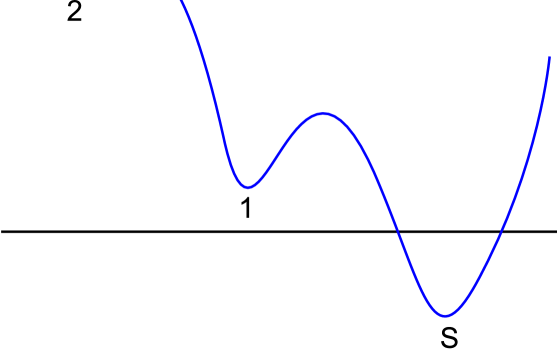
Figure 2: A potential with two dS minima and a sink.

Let us consider a simple model describing two dS minima and one AdS minimum (denoted by 1, 2, and S in Fig. 2). Here, as in the rest of this paper, we work in comoving co-ordinates. To get a visual understanding of the process of bubble formation in comoving coordinates, one may paint black all of the parts corresponding to one of the two dS states, and paint white the parts in the other dS state. Then, in the absence of sinks in the landscape, the multiverse will become populated by white and black bubbles of all possible sizes. Asymptotically, it will approach a stationary regime – on average becoming gray, with the level of gray becoming asymptotically constant. Suppose now that some parts of the universe may tunnel to a state with a negative cosmological constant. These parts will collapse, so they will not return to the initial dS vacua. If we paint such parts red, then the universe, instead of reaching a constant shade of gray, eventually will look completely red.

To describe this process, instead of the detailed balance equation (7) one should use the “vacuum dynamics” equations [20, 26]:

$$\dot{P}_{1}=-J_{1s}-J_{12}+J_{21}\ ,$$ (10)

$$\dot{P}_{2}=-J_{2s}-J_{21}+J_{12}\ .$$ (11)

Here $J_{ij}=P_{j}\,\Gamma_{ji}$, where $\Gamma_{ji}$ is the decay rate of the vacuum $j$ to bubbles of vacuum $i$. In particular, $J_{1s}=P_{1}\,e^{-C_{1}}$ is the probability current from the lower dS vacuum to the sink, i.e. to a collapsing universe, or to a Minkowski vacuum, $J_{2s}=P_{2}\,e^{-C_{2}}$ is the probability current from the upper dS vacuum to the sink, $J_{12}=P_{1}\,e^{-{\bf S_{1}}+|S(\phi)|}$ is the probability current from the lower dS vacuum to the upper dS vacuum, and $J_{21}=P_{2}\,e^{-{\bf S_{2}}+|S(\phi)|}$ is the probability current from the upper dS vacuum to the lower dS vacuum. Combining this all together, gives us the following set of equations for the probability distributions:

$$\dot{P}_{1}=-P_{1}\,(\Gamma_{1s}+\Gamma_{12})+P_{2}\,\Gamma_{21}\ ,$$ (12)

$$\dot{P}_{2}=-P_{2}\,(\Gamma_{2s}+\Gamma_{21})+P_{1}\,\Gamma_{12}\ .$$ (13)

We ignore here possible sub-exponential corrections, which appear, e.g., due to the difference in the initial size of the bubbles etc.

Because of the decay to the sink, $P_{1}$ and $P_{2}$ gradually become exponentially small. But this does not mean that the whole universe goes to the sink: The physical volume of white and black parts of the universe continues growing exponentially, in the regime of eternal inflation. One of the ways to account for this growth is to slice the universe by hypersurfaces of time $t$ measured in units of $H^{-1}$. In this case, volume of all parts of the universe during time $\Delta t=1$ grows $e^{3}$ times. One can describe this effect by adding the terms $3P_{i}$ to the r.h.s. of Eqs. (12), (13) [27]. As a result, the functions $P_{i}$ describing the total volume of the different dS vacua will grow exponentially even in the presence of the sink (if the rate of decay to the sink is not too large). In this case, the functions $P_{i}$ will correspond to the ’pseudo-comoving’ probability distribution [27]. In this paper we will be interested only in the ratios of the volumes of dS spaces, $P_{i}/P_{j}$. These ratios are not affected by the overall growth of all parts of the universe, and therefore the ratios $P_{i}/P_{j}$ are the same for the comoving and pseudo-comoving probability distributions. Therefore for simplicity we will not add the terms $3P_{i}$ to the r.h.s. of our equations, i.e. we will study comoving probabilities.

To analyze the solutions of equations (12) and (13), let us first understand the relations between their parameters. Since entropy of dS space is inversely proportional to energy density, the entropy of the lower level is highest, ${\bf S_{1}}>{\bf S_{2}}$. As the tunneling is exponentially suppressed, we have ${\bf S_{2}}>|S(\phi)|$, so we obtain a hierarchy ${\bf S_{1}}>{\bf S_{2}}>|S(\phi)|$, and therefore $\Gamma_{12}\ll\Gamma_{21}\ll 1$. We will often associate the lower vacuum with our present vacuum state, where $S_{1}\sim 10^{{120}}$.

For simplicity, we will study here the possibility that only the lower vacuum can tunnel to the sink, $\Gamma_{2s}=0$. The two equations (12) and (13) can then be solved exactly to give the general solution

$$P_{1}=C_{1}e^{-\frac{1}{2}(\Gamma_{12}+\Gamma_{1s}+\Gamma_{21})(t-t_{0})}\cosh\left[\frac{A}{2}(t-t_{0})\right],$$ (14)

where $C_{1}$ and $t_{0}$ are constants and $A^{2}\equiv(\Gamma_{12}+\Gamma_{1s}+\Gamma_{21})^{2}-4\Gamma_{1s}\Gamma_{21}.$ Substituting back into the $\dot{P}_{1}$ equation then gives the ratio

$$\frac{P_{2}}{P_{1}} = \frac{\Gamma_{12}-\Gamma_{21}+\Gamma_{1s}+A\tanh\left[\frac{A}{2}(t-t_{0})\right]}{2\Gamma_{21}}$$ (15)

$$\rightarrow \frac{\Gamma_{12}-\Gamma_{21}+\Gamma_{1s}+A}{2\Gamma_{21}}$$

as $t\rightarrow\infty$. These solutions show us that in a comoving coordinate system, in the presence of a sink, both of $P_{1}$ and $P_{2}$ are decaying, whilst their ratio approaches a constant value (i.e. their rates of decay become equal).

One may consider two interesting regimes, providing two very different types of solution. Suppose first that $\Gamma_{1s}\ll\Gamma_{21}$, i.e. the probability to fall to the sink from the lower vacuum is smaller than the probability of the decay of the upper vacuum. In this case one recovers the result obtained without the sink in the previous section:

$${P_{2}\over P_{1}}={\Gamma_{12}\over\Gamma_{21}}=e^{{\bf S_{2}}-{\bf S_{1}}}\ll 1.$$ (16)

It is interesting that this thermal equilibrium is maintained even in the presence of a sink if $\Gamma_{1s}\ll\Gamma_{21}$. Note that the required condition for thermal equilibrium is not $\Gamma_{1s}\ll\Gamma_{12}$, as one could naively expect, but rather $\Gamma_{1s}\ll\Gamma_{21}$. We will call such sinks narrow.

Now let us consider the opposite regime, and assume that the decay rate of the uplifted dS vacuum to the sink is relatively large, $\Gamma_{1s}\gg\Gamma_{21}$, which automatically means that $\Gamma_{1s}\gg\Gamma_{12}$. In this “wide sink” regime the solution of Eq. (15) is

$${P_{2}\over P_{1}}={\Gamma_{1s}\over\Gamma_{21}}=e^{{\bf S_{2}}-|S(\phi)|-C_{1}}\approx e^{{\bf S_{2}}-|S(\phi)|}\gg 1,$$ (17)

i.e. one has an inverted probability distribution. This result has a simple interpretation: if the “thermal exchange” between the two dS vacua occurs very slowly as compared to the rate of the decay of the lower dS vacuum, then the main fraction of the volume of the dS vacua will be in the state with the higher energy density, because everything that flows to the lower level rapidly falls to the sink.

4 Is the Landscape Transversable?

Before discussing the details of how AdS sinks can effect thermal structure in the landscape, we will make a note of another scenario that can arise in their presence: The separation of the landscape into disconnected regions, or islands.

Consider the simple potential shown in Fig. 3. One may naively expect that all energetically favorable transitions between vacua should occur; however, this may not be the case in the presence of sinks. In the absence of gravity we know that quantum mechanical tunneling can only occur from higher energy vacua to lower energy ones. In such a picture all vacua slowly tunnel to lower and lower energy, until they eventually end up in the lowest energy ground state. Including the effects of gravity changes this situation by allowing the possibility of tunneling upwards, to higher energy. Although going upwards is less probable than going down, between any two vacua, the system soon settles down into a situation where the fluxes going up and down are equal. This behavior occurs when the population in the lower energy state far exceeds the number in the high energy state, compensating the unlikeliness of jumping upwards by increasing the number of vacua that could potentially make this transition. This process is known as recycling, and, for a system of dS vacua only, allows the whole system to approach thermal equilibrium, where the ratios of occupation numbers of any two vacua are given by the equilibrium ratios (9).

AdS and Minkowski sinks, which can be tunneled to, but not back from, spoil this recycling mechanism and can disrupt the global thermal structure that would otherwise exist. One manifestation of this effect is the altered occupation fractions $P_{i}/P_{j}$, discussed in the previous section; another is the possibility of these sinks separating the landscape into isolated regions, which may be in thermal equilibrium internally, but not with each other. We call such regions ‘islands’.

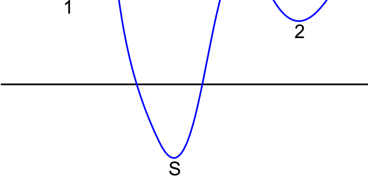
Figure 3: A potential with two dS minima seperated by a sink.

Fig. 3 shows a simple situation which may occur in the landscape; two dS vacua with an AdS sink between them. If tunneling is allowed between the two dS vacua, then thermal equilibrium between them can occur. Conversely, if tunneling is not allowed then these two vacua will be totally isolated from one another.

Consider first the possibility of a Coleman-De Luccia transition from vacuum 1 to vacuum 2. As was shown in [31], the CDL instantons exist only for $V^{\prime\prime}\gtrsim V$, where tunneling is usually assumed to occur from one side of a potential barrier to the other, as in Fig. 1. The scalar field then rolls down the potential to the minimum, where reheating may occur if conditions are right. For the situation shown in Fig. 3, however, such rolling will be down to an AdS minimum, which corresponds to a collapsing open universe. One may speculate about the possibility of a tunneling from a collapsing space, or about the re-emergence of the universe after the collapse, but we do not know how to study this regime in a controllable way. Alternatively, one may try to find the CDL instantons describing a direct tunneling from vacuum 1 to vacuum 2, jumping over the AdS minimum.

On the other hand, if we consider $V^{\prime\prime}\ll V$, then the CDL instantons do not exist. In this case we still have the Hawking-Moss instanton, and its interpretation in stochastic inflation. However, according to the stochastic interpretation of the HM tunneling, there can be no tunneling directly from 1 to 2. Recall that we view this scenario as representing the scalar field tunneling to the top of the barrier through a sequence of quantum jumps and subsequently rolling down to an adjacent vacuum. Clearly this is not a plausible transition between 1 and 2, since the only adjacent vacuum is the central AdS sink.

Thus, in general one may encounter situations where it is not possible to travel from one part of the landscape to another. However, it may happen that whereas the probability of the transitions discussed above may be extremely small, they cannot be strictly forbidden; our ‘no trespassing’ result may be just a consequence of the approximation used to study such processes. Moreover, considering a multi-dimensional potential with many moduli and fluxes will also add complexity, as tunneling between vacua 1 and 2 could occur in the other dimensions. With an increasing number of dimensions it becomes increasingly likely that tunneling will be able to occur either directly between 1 and 2, or via some intermediary vacuum. Despite these caveats, we find it interesting that the existence of sinks allows for the possibility of the landscape being separated into isolated islands.

In the following section we will consider the possibility of tunneling events directly between two islands, separated by a sink. Such events could be due to a direct tunneling via the Coleman-De Luccia instantons in the regime $V^{\prime\prime}>V$, or due to a sequence of the tunneling events though intermediate vacua. We will show that even if these events are allowed and the islands are not totally isolated, they may still be thermally isolated from one another as the sink can disrupt the equilibrium that would otherwise exist. However, our analysis leads us to believe that if the number of dimensions in the landscape is large enough then the existence of sinks will not be able to disrupt the tunneling in all of these dimensions, and thermal contact will therefore be maintained. Furthermore, the ‘tortoise and the hare’ behavior we find indicates that if a single high-energy vacuum is allowed to decay to vacua on each of the islands then this vacuum will act as a bridge, restoring thermal contact. For a landscape with very many vacua and dimensions, it therefore seems implausible that thermally isolated regions should occur. We discuss this in more detail below.

5 Non-Trivial Thermal Structure in the Landscape

In this section we will present our results and analysis of more general situations than the simple one shown in Fig. 2. We explore the situations in which thermal equilibrium (which is to say, detailed balance) between vacua is disturbed. We hope that this discussion will be of interest to a wider audience, and can be understood without having to follow lengthy calculations. The interested reader can then proceed to the appendix, where the mathematical minutiae are given.

5.1 The General Equation

For a system of $n$ vacua and a single sink we can describe the evolution of the probability measures, $P$, by:

$$\frac{dP_{i}}{dt}=-\sum_{j\neq i}\Gamma_{ij}P_{i}+\sum_{j\neq i}\Gamma_{ji}P_{j}-\Gamma_{is}P_{i}.$$ (18)

This equation is completely general: Single sinks to which many vacua can decay with differing amplitudes, and multiple sinks to which individual vacua can decay (again with differing amplitudes) amount to the same thing. The exact form of the general solution to this set of equations is found in Appendix A.1:

$$P_{i}=\sum_{j}c_{ij}e^{-m_{j}t}\ ,$$

where the $c_{ij}$ are constants of integration, and the $m_{j}$ are constants formed from the transition rates, $\Gamma$. All $P_{i}$ have the same functional form, and their coefficients $c_{ij}$ are related by factors which are functions of the $\Gamma$s only.

At late times the ratios between different vacua then asymptote to the constant values:

$$r_{ij}\equiv\lim_{t\rightarrow\infty}\frac{P_{i}}{P_{j}},$$ (19)

which can easily be found, using the solutions for $P_{i}$. Of course, finding solutions in a generic landscapes is not easy, so we will restrict ourselves to a number of simple examples.

In section 3 we found the solution for the potential illustrated in Fig. 2, and proceeded to find the asymptotic limit of the ratio $P_{2}/P_{1}$ as $t\rightarrow\infty$. We now find simple estimates for the asymptotic form of the ratios $P_{i}/P_{j}$ in more generic situations.

5.2 An Extended 1D Potential

Consider now the extended one-dimensional potential in Fig. 4. Here we allow transitions between neighboring de Sitter minima in both directions, and transitions from 1 to the AdS sink. The equations determining the vacuum dynamics, and their solutions, are given in Appendix A.2.1.

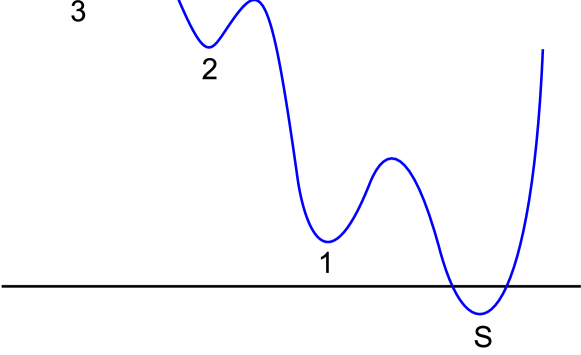
Figure 4: A one-dimensional potential with three positive and one negative minima

For definiteness, we will assume that $V_{3}>V_{2}>V_{1}$, and therefore $\Gamma_{32}>\Gamma_{23}$, and $\Gamma_{21}>\Gamma_{12}$.

Firstly, when $\Gamma_{1s}\ll\Gamma_{21}$, we find:

$$\frac{P_{1}}{P_{2}}\simeq\frac{\Gamma_{21}}{\Gamma_{12}}\gg 1\qquad\text{and}\qquad\frac{P_{3}}{P_{2}}\simeq\frac{\Gamma_{23}}{\Gamma_{32}}\ll 1.$$

In this limit the thermodynamic ratios (9) are maintained because $\Gamma_{21}\gg\Gamma_{12}$ and $\Gamma_{32}\gg\Gamma_{23}$. When $\Gamma_{1s}\gg\Gamma_{21}$ and $\Gamma_{21}\ll\Gamma_{32}$, we find:

$$\frac{P_{1}}{P_{2}}\simeq\frac{\Gamma_{21}}{\Gamma_{1s}}\ll 1\qquad\text{and}\qquad\frac{P_{3}}{P_{2}}\simeq\frac{\Gamma_{23}}{\Gamma_{32}}\ll 1.$$

Here the thermal ratio of $P_{1}$ to $P_{2}$ is broken, whilst that of $P_{2}$ to $P_{3}$ is maintained. Lastly, when $\Gamma_{1s}\gg\Gamma_{21}$ and $\Gamma_{21}\gg\Gamma_{32}$, we find:

$$\frac{P_{1}}{P_{2}}\simeq\frac{\Gamma_{21}}{\Gamma_{1s}}\ll 1\qquad\text{and}\qquad\frac{P_{3}}{P_{2}}\simeq\frac{\Gamma_{21}}{\Gamma_{32}}\gg 1.$$

Now the thermal ratio of $P_{1}$ to $P_{2}$, and the ratio of $P_{2}$ to $P_{3}$, is broken.

Whilst the equations with three dS vacua are more complicated than the case for two, it now appears that the interpretation can be straightforwardly extended. The ratio $P_{2}/P_{1}$ is not affected (to leading order) by the presence of the extra minimum, and again its form is prescribed by the magnitude of $\Gamma_{1s}$ relative to $\Gamma_{21}$. The new ratio $P_{3}/P_{2}$ is found to take its thermal value if $P_{2}/P_{1}$ has a thermal ratio. If $P_{2}/P_{1}$ has its thermal ratio broken then the rate $\Gamma_{12}$ becomes negligible, and the minimum 1 acts as a sink for the remaining two dS vacua. The ratio $P_{3}/P_{2}$ can then be calculated as if they were a system of two dS spaces with vacuum 2 being allowed to decay to a sink.

5.3 A Simple “Multidimensional” Landscape

We now wish to consider the case of a multi-dimensional potential, which we expect to be a slightly more realistic model of the landscape. Again, we work with an extension of the simple case of two dS minima and one sink that was given in section 3. Now we consider the potential shown in Fig. 5. Here transitions are allowed between the minima labeled 2 and 3 and the lower minima 1, which is allowed to decay directly to the sink. This setup models a simple potential with more than one dimension, i.e. with more than just pairwise connections between vacua. The equations for this potential are given, and solved, in Appendix A.2.2.

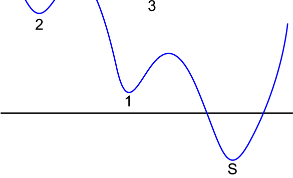
Figure 5: A multi-dimensional potential with three positive and one negative minima

Under the reasonable assumptions that $\Gamma_{21}\gg\Gamma_{12}$ and $\Gamma_{31}\gg\Gamma_{13}$, we find:

$$\frac{P_{2}}{P_{1}}\simeq\frac{\Gamma_{12}}{\Gamma_{21}}\ll 1\qquad\text{and}\qquad\frac{P_{3}}{P_{1}}\simeq\frac{\Gamma_{13}}{\Gamma_{31}}\ll 1$$

when $\Gamma_{21}$ and $\Gamma_{31}\gg\Gamma_{1s}$; whilst for $\Gamma_{1s}$ and $\Gamma_{31}\gg\Gamma_{21}$ we find:

$$\frac{P_{2}}{P_{1}}\simeq\frac{\Gamma_{1s}}{\Gamma_{21}}\gg 1\qquad\text{and}\qquad\frac{P_{3}}{P_{1}}\simeq\frac{\Gamma_{13}}{\Gamma_{31}}\ll 1.$$

The case $\Gamma_{1s}$ and $\Gamma_{21}\gg\Gamma_{31}$ can be found by symmetry from the above expressions, under the transcription 2$\leftrightarrow$3.

These results have a straightforward, but slightly counter-intuitive, interpretation. When the sink is narrow with respect to the transition rate $\Gamma_{21}$, as well as the rate $\Gamma_{31}$, the thermal ratios of both $P_{2}$ and $P_{3}$, with respect to $P_{1}$, are maintained, as expected. When the sink is wide with respect to one of the $\Gamma$s (and narrow with respect to the other), one of $P_{2}$ and $P_{3}$ will maintain its thermal ratio whilst the other does not, again, as expected. One could expect that when the sink is wide with respect to all other transition rates, all dS vacua will be out of equilibrium. Surprisingly, we have found that even in this case only one of the upper vacua is out of its thermal ratio with $P_{1}$, and the other is not. Furthermore, the vacuum that is taken out of thermal equilibrium with $P_{1}$ is the one with the slowest rate of decay.

We interpret this in the following way: If the sink is wide with respect to all other transition rates, then the magnitude of $P$ in the vacuum that decays the quickest will quickly become very small. The slowest decaying vacuum, despite the fact that the rate $\Gamma$ is smaller, will then be the source of the majority of the probability flux at late-times. The small flux that is required to keep the faster decaying vacuum in its thermal ratio with the lower vacuum is then maintained by the flux from the slower decaying vacuum, which is forced out of its thermal ratio by the sink.

The picture of the slowest decaying vacuum dominating the behavior of the universe may seem counter intuitive, but in fact it has a very simple interpretation: Those who want to survive in a desert (i.e. near wide sinks) should save water.

Numerical simulations show that this behavior extends to $i>2$ vacua decaying into a single lower vacuum, which decays to a sink. If the sink is narrow with respect to all of the other transition rates, then the asymptotic ratios $P_{i}/P_{1}$ approach the thermal ratios that they would have in the absence of the sink. If the sink is wide with respect to any or all of the transition rates to the higher vacua, then it is only the slowest decaying vacuum that is forced out of its thermal equilibrium with the lower vacuum. In this case, the out-of-equilibrium slowest decaying vacuum will feed all other vacua, which will be in a state of thermal equilibrium with each other.

5.4 Multiple Sinks

We now have some ideas on how to extend the simple model of two dS spaces and one AdS space to more general models with multiple dimensions and higher vacua. However, so far we have only studied potentials in which one vacuum is allowed to decay to AdS space. In a realistic model of the landscape it is likely that many vacua will be allowed to decay in this way, and it is the effects of this which we now study.

5.4.1 2 dS and 2 AdS

The potential with two dS minima, shown in Fig. 2, can be simply extended to allow both of the dS minima to decay to sinks. This situation is solved in Appendix A.2.3. Again, we assume $\Gamma_{12}\ll\Gamma_{21}$.

It can now be shown that if both the sinks are narrow ($\Gamma_{js}\ll\Gamma_{ij}$) then the ratio $P_{2}/P_{1}$ maintains its thermal value, to leading order. Similarly, if one sink is narrow, and the other is wide ($\Gamma_{js}\gg\Gamma_{ij}$), then the leading order terms are the same as in the absence of the narrow sink. Now, if both sinks are wide then the ratio $P_{2}/P_{1}$ is determined by the wider sink. For example, if we have the hierarchy $\Gamma_{1s}\gg\Gamma_{2s}\gg\Gamma_{21}$, then

$$\frac{P_{2}}{P_{1}}\simeq\frac{\Gamma_{1s}}{\Gamma_{21}}\ ,$$

whilst for $\Gamma_{2s}\gg\Gamma_{1s}\gg\Gamma_{21}$, we have

$$\frac{P_{2}}{P_{1}}\simeq\frac{\Gamma_{12}}{\Gamma_{2s}}\ .$$

5.4.2 3 dS and 2 AdS

We may also consider the case of a single higher vacuum that can decay to multiple lower vacua, which are, in turn, able to subsequently decay to sinks. We will model this situation by considering a potential such as that shown in Fig. 6, where the vacua labeled 1 and 3 are allowed to decay to sinks. The equations for this potential are investigated in Appendix A.2.4. We now have the heirarchy $\Gamma_{21}\gg\Gamma_{12}$ and $\Gamma_{23}\gg\Gamma_{32}$.

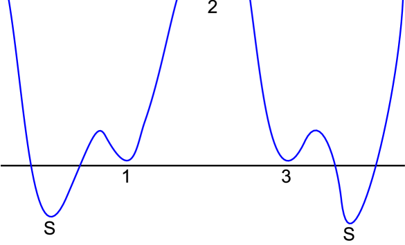
Figure 6: A potential with three positive minima, the lower two of which can decay to sinks.

When both sinks are narrow, $\Gamma_{1s}\ll\Gamma_{21}$ and $\Gamma_{3s}\ll\Gamma_{23}$, the thermal ratios

$$\frac{P_{1}}{P_{2}}=\frac{\Gamma_{21}}{\Gamma_{12}}\gg 1\qquad\text{and}\qquad\frac{P_{3}}{P_{2}}=\frac{\Gamma_{23}}{\Gamma_{32}}\gg 1\qquad$$

are maintained. For one narrow sink and one wide ($\Gamma_{is}\gg\Gamma_{2i}$) the narrow sink becomes irrelevant, and the problem reduces to the extended one-dimensional potential considered above.

For two wide sinks, if we take $\Gamma_{1s}\gg\Gamma_{3s}$, without loss of generality, then we always have the ratio

$$\frac{P_{1}}{P_{2}}=\frac{\Gamma_{21}}{\Gamma_{1s}}\ll 1.$$

The second ratio, $P_{3}/P_{2}$, is then determined by the relative magnitudes of $\Gamma_{3s}$ and $\Gamma_{21}$. If $\Gamma_{3s}\gg\Gamma_{21}$, then we have

$$\frac{P_{3}}{P_{2}}=\frac{\Gamma_{23}}{\Gamma_{3s}}\ll 1;$$

whilst for $\Gamma_{3s}\ll\Gamma_{21}$ we have

$$\frac{P_{3}}{P_{2}}=\frac{\Gamma_{21}}{\Gamma_{32}}\gg 1.$$

This can be understood in terms of the previous example of two dS spaces, both connected to sinks. If the probability charge in vacuum 1 is rapidly depleted by the fast decay rate to the sink, $\Gamma_{1s}$, then vacuum 1 will subsequently act as a sink for the remaining two vacua. If decays to this new effective sink, $\Gamma_{21}$, are faster than the decay rate $\Gamma_{3s}$, then this new sink will dominate. Otherwise, $\Gamma_{3s}$ will dominate.

5.4.3 Islands

Consider the potential shown in Fig. 7. Here there are two dS minima which are allowed to decay to a sink. (Each of the lower dS vacua could be considered to decay to different sinks, or to a common sink, the results are the same). We have also included two higher vacua connected to the lower ones, and transitions are allowed between the two lower minima. Here we hope to see the effects of having more than one vacuum decaying to a sink. We expect that the presence of the second sink will complicate matters and allow for the possibility of two ‘islands’ that are in thermal equilibrium internally, but not with each other.

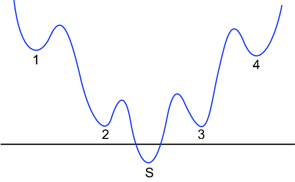
Figure 7: A potential with two positive minima that are allowed to decay to anti-de Sitter space.

With our knowledge of the general solution, we know that the asymptotic attractor solutions will be of the form:

$$P_{2} = c_{1}e^{-mt}\,,$$

$$P_{3} = nc_{1}e^{-mt}=nP_{2}\ .$$

As shown below, under the reasonable assumption that $\Gamma_{34}\ll\Gamma_{43}$ and $\Gamma_{21}\ll\Gamma_{12}$, we find three possible values of $n$ and $m$ in Appendix A.2.5. In order to choose which solution for $n=P_{3}/P_{2}$ is the relevant one, for a given set of $\Gamma$s, we must evaluate which $m$ is the smallest. This $m$ will correspond to the slowest decaying mode, which dominates in the limit $t\rightarrow\infty$; the corresponding $n$ will then give the appropriate asymptotic ratio of $P_{2}/P_{3}$. A flow chart is given in Appendix B, which can be used to quickly identify the relevant asymptotic form of $n$ for any given set of $\Gamma$s.

From the flow chart it can be seen that a necessary condition to maintain a thermal ratio between vacua 2 and 3 is that either $\Gamma_{32}\gg\Gamma_{3s}$ or $\Gamma_{23}\gg\Gamma_{2s}$. A sufficient condition for maintaining this ratio is either $\Gamma_{23}$ or $\Gamma_{32}\gg\Gamma_{2s}$ and $\Gamma_{3s}$. Conversely, a necessary condition for breaking the thermal ratio between 2 and 3 is either $\Gamma_{2s}$ or $\Gamma_{3s}\gg\Gamma_{23}$ and $\Gamma_{32}$; whilst a sufficient condition is given by $\Gamma_{2s}$ and $\Gamma_{3s}\gg\Gamma_{23}$ and $\Gamma_{32}$.

Two sets of solutions are relatively simple:

$$n_{1} = \frac{\Gamma_{23}}{\Gamma_{32}+\Gamma_{3s}}\ ,$$

$$n_{2} = \frac{\Gamma_{23}+\Gamma_{2s}}{\Gamma_{32}}\ ,$$

with the corresponding values of $m$ being given by

$$m_{1} = \Gamma_{12}\ ,$$

$$m_{2} = \Gamma_{43}\ .$$

The expressions for $m_{3}$ and $n_{3}$ are somewhat more complicated, but they can be simplified depending on the relative magnitudes of $\Gamma_{23}$, $\Gamma_{32}$, $\Gamma_{2s}$ and $\Gamma_{3s}$. If $\Gamma_{23}$ or $\Gamma_{32}$ are the fastest of these rates then the leading order contributions to $m_{3}$ and $n_{3}$ are

$$n_{3a}\simeq\frac{\Gamma_{23}}{\Gamma_{32}}\qquad\text{and}\qquad m_{3a}\simeq\frac{\Gamma_{2s}\Gamma_{32}+\Gamma_{3s}\Gamma_{23}}{\Gamma_{23}+\Gamma_{32}},$$

if $\Gamma_{2s}$ is the fastest then

$$n_{3b}\simeq\frac{\Gamma_{2s}}{\Gamma_{32}}\qquad\text{and}\qquad m_{3b}\simeq\Gamma_{32}+\Gamma_{3s}$$

and, similarly, if $\Gamma_{3s}$ is the fastest then

$$n_{3c}\simeq\frac{\Gamma_{23}}{\Gamma_{3s}}\qquad\text{and}\qquad m_{3c}\simeq\Gamma_{23}+\Gamma_{2s}\ .$$

We will now consider the significance of each of these three solutions. We take solutions $n_{1}$ and $m_{1}$ as corresponding to the situation in which the probability flux is sourced by the slowly decaying vacuum 1; solutions $n_{2}$ and $m_{2}$ correspond to the situation in which vacuum 4 is the slowest decaying, and therefore sources the probability flux; and solutions $n_{3}$ and $m_{3}$ correspond to the situation where the majority of the probability flux is from the lower vacua, 2 and 3. This interpretation is supported by the various values of $m$. For $m_{1}$ and $m_{2}$ it can be seen immediately that the asymptotic rate of decay of the $P_{i}$ is prescribed by the rate of decay from 1 to 2 or from 4 to 3, respectively. This strongly suggests that the vacuum dynamics of the systems corresponding to these solutions are dominated by the flux out of vacua 1 and 4.

The interpretation of the $m_{3}$/$n_{3}$ solution is a little less straightforward due to its more complicated form. When the rate of decay $\Gamma_{2s}$ is fast, $m_{3b}$ is the relevant solution. It can be seen that $m_{3b}$ is determined by the probability flux out of vacuum 3 (recall that $\Gamma_{34}$ has been neglected). By symmetry, when $\Gamma_{3s}$ is large $m_{3c}$ is the relevant solution, which is given by the rate of decay out of vacuum 2. When both rates of decay to the sink are small, $m_{3a}$ is the relevant solution, which can be seen to be some weighted flux out of both of the vacua 2 and 3 (analogous to the ‘reduced mass’ of two body dynamics). This justifies the above statement that the solutions $m_{3}$ and $n_{3}$ correspond to a system which is dominated by the flux out of vacua 2 and/or 3.

We again see that the asymptotic form of the ‘vacuum dynamics’ is not prescribed by the fastest decaying vacua, as may have been naively expected, but by the slowest. These vacua hold the majority of the comoving volume at late times, and so dominate the late time evolution of the universe.

The late-time evolution of $P_{2}$ and $P_{3}$ straightforwardly gives the behavior of $P_{1}$ and $P_{4}$. Using the notation $p\equiv P_{1}/P_{2}$ and $r\equiv P_{4}/P_{3}$, we obtain

$$p_{1}\neq\frac{\Gamma_{21}}{\Gamma_{12}},\qquad p_{2}=\frac{\Gamma_{21}}{\Gamma_{12}}\qquad\text{and}\qquad p_{3}=\frac{\Gamma_{21}}{\Gamma_{12}}$$

and

$$r_{1}=\frac{\Gamma_{34}}{\Gamma_{43}},\qquad r_{2}\neq\frac{\Gamma_{34}}{\Gamma_{43}}\qquad\text{and}\qquad r_{3}=\frac{\Gamma_{34}}{\Gamma_{43}},$$

where subscripts $i$ denote that the solution corresponds to $m_{i}$ and $n_{i}$. It can be seen that if the probability charge is being held in vacua 1 or 4, then that vacuum is out of its thermal ratio with the lower vacuum to which it can decay, and that the two vacua on the other side of the sink are in their thermal ratio. If the probability charge is being held in either or both of the lower vacua, then both of the higher vacua have thermal ratios with their respective lower vacua.

Since we have here a large variety of possibilities, let us single out some of the most interesting regimes. Suppose first that $\Gamma_{23}=\Gamma_{32}=0$, as discussed in Section 4. In this case, in the wide sink regime, vacua 1 and 2 will be out of thermal equilibrium with each other, vacua 3 and 4 will be out of thermal equilibrium with each other, and branches (1,2) and (3,4) will be totally disconnected.

Now let us establish some contact between these branches. If $\Gamma_{23}$ and $\Gamma_{32}$ are sufficiently small, we will have branches (1,2) and (3,4) out of thermal equilibrium with each other. If vacuum 1 has the slowest decay rate among all vacua, it will be out of equilibrium with vacuum 2. However, in this case vacuum 4 will be in thermal equilibrium with vacuum 3, even if $\Gamma_{23}$ and $\Gamma_{32}$ are extremely small. Note that the transition to vanishing $\Gamma_{23}$ and $\Gamma_{32}$ is discontinuous. This paradoxical situation is similar to the one encountered earlier: The slowest decaying vacuum dominates the evolution of other domains, but this vacuum becomes irrelevant if it totally decouples from other vacua. Other possibilities can be read from the flow chart in Appendix B.

The model discussed in this section shows explicitly that tunneling to sinks can break the detailed balance between vacua that would otherwise keep different regions of the landscape in thermal contact. This provides a mechanism by which the landscape can be separated into different thermally isolated parts, each with a different ‘temperature’. In a landscape with high enough dimensionality there may be more than one decay channel between 2 and 3. This will make it more likely that thermal contact will be maintained between various parts of the landscape.

6 Discussion

We have, in the course of this work, carried out a detailed exploration of some toy models of the landscape, and studied their thermal properties. Whilst these models are somewhat limited in their scope, they have revealed to us a rich, and sometimes counter-intuitive structure.

In general, it appears that a necessary condition for the disruption of thermal ratios between vacua is a rapid rate of decay to an AdS space – a wide sink. Intriguingly, however, once this condition is met, the late-time behavior of the system is controlled by the slowest of the tunneling processes. For example, when we considered a simplified version of a multi-dimensional landscape with a single sink (Section 5.3) we found that only the slowest decaying vacuum was shifted from its thermal ratio with the lower vacuum: All other ratios remained in thermal equilibrium. We interpret this as being due to the more rapidly decaying vacua quickly depleting their populations, leaving the slowest decaying vacuum to be the primary source of probability flux. The late-time thermal behavior of the multiverse is then determined by the weakest transitions – transitions that would otherwise be irrelevant in the absence of a sink, or if we took the limit of their rate going to zero.

We see a similarly interesting interplay in our “islands” example in Section 5.4.3. Here, once thermal equilibrium is disrupted by a wide sink, the late-time behavior of the system is again determined by the slowest decaying vacuum. In this example the sink can break the thermal contact between different regions, leaving several thermally disconnected ‘islands’.

In a more complex model there may exist intermediate vacua that can act as bridges, restoring thermal contact between islands. Such vacua would be required to be able to decay to both of the islands, with a non-negligible rate. As we have shown, quickly decaying vacua are likely to be in thermal equilibrium with the lower vacua to which they are allowed to decay. It may happen that for a realistic landscape with many dimensions and very many vacua, the thermally isolated regions will be relatively rare. However, in order to verify this conjecture one would need to study simultaneously a disruptive effect of a very large number of sinks and a restoring effect of a very large number of bridges.

We anticipate that further exploration along the lines of this paper may reveal still more interesting features, allowing us a more complete and better understood picture of the landscape.

Acknowledgments

We are grateful to T. Banks, R. Bousso, R. Easther, B. Freivogel, S. Shenker, L. Susskind and A. Vilenkin for valuable discussions. This work is supported by NSF grant PHY-0244728. TC is supported by a Lindemann fellowship.

Appendix A Solving the Equations

In this appendix we will elaborate on some mathematical details of the results given in the main body of the text.

A.1 General Solution

As discussed in section 5, the equations governing the evolution of some set of $P$s are:

$$\frac{dP_{i}}{dt}=-\sum_{j\neq i}\Gamma_{ij}P_{i}+\sum_{j\neq i}\Gamma_{ji}P_{j}-\Gamma_{is}P_{i}.$$

The first term on the right hand side gives the flux out of the state denoted by $P_{i}$ to all the other $P_{j}$, the second gives the flux into $P_{i}$ and the third gives the flux out of $P_{i}$ and into the sink. For $n$ different $P$s, we have a set of $n$ coupled first order ordinary differential equations. Such a set of equations can be manipulated into a single linear $n$th order equation, for any one particular $P_{i}$, of the form:

$$\sum_{j}^{n}a_{j}\frac{d^{j}P_{i}}{dt^{j}}=0\ .$$ (20)

The coefficients $a_{j}$ can be written in terms of the transition rates, $\Gamma$. This equation has the general solution

$$P_{i}=\sum_{j}^{n}c_{j}e^{-m_{j}t}\ ,$$ (21)

where the $c_{j}$ are constants of integration and the constants $m_{j}$ are the $n$ roots of the $n$th order polynomial $\sum_{j}^{n}a_{j}m^{j}=0$. All other $P_{i}$ can then be seen to have the same functional form, by substitution back into the original set of equations (18). The coefficients of the different modes of these other $P_{i}$ will be completely determined in terms of $c_{j}$ and the $\Gamma$s. This gives the general solution to (18), for all $P_{i}$, with $n$ arbitrary constants.

At late times the dominant mode in the solution (21) will be the one with the smallest exponent, $m$. As all the $P$s have the same functional forms, the same mode will dominate the evolution of each $P$ at late times, and so the ratios $P_{i}/P_{j}$ will asymptotically approach constant values. The form of the dominant mode can now be calculated in terms of the constant ratios $q_{ij}\equiv P_{i}/P_{j}$ by adding all the equations (18) to get

$$\Big{(}1+\sum_{i}q_{ij}\Big{)}\dot{P}_{j}=-\Big{(}\Gamma_{js}+\sum_{i}\Gamma_{is}q_{ij}\Big{)}P_{j}\ ,$$ (22)

which can be integrated to

$$\ln P_{j}=-\frac{(\Gamma_{js}+\sum_{i}\Gamma_{is}q_{ij})}{(1+\sum_{i}q_{ij})}(t-t_{0})\ ,$$ (23)

where $t_{0}$ is an arbitrary constant. We now see that the smallest value of $m$, which corresponds to the dominant term as $t\rightarrow\infty$, is given by

$$m=\frac{(\Gamma_{js}+\sum_{i}\Gamma_{is}q_{ij})}{(1+\sum_{i}q_{ij})}<0.$$ (24)

Therefore the real part of all of the roots $m_{i}$ are $>0$, and all the modes are decaying.

We now know that the late-time attractor solution for each of the $P$s is an exponentially decaying function, and that this rate of decay is the same for each $P$. This allows us to work out the constant ratios $q_{ij}$, that are asymptotically approached as $t\rightarrow\infty$. Taking the mode with the smallest $m$ and substituting it back into (18) gives us a set of $n-1$ algebraic equations which can be solved for the $n-1$ unknown ratios $q_{ij}$. The asymptotic form of the $P$s is now, up to a normalization, completely solved for.

A.2 Details of Particular Solutions

Here we will provide the equations that were used to find the results in the main body of the text, above. We will assume that all transition rates, $\Gamma$, are orders of magnitude different from each other.

A.2.1 An Extended 1D Potential

The equations governing the system shown in Fig. 4 are given by

$$\dot{P}_{1} = -(\Gamma_{12}+\Gamma_{1s})P_{1}+\Gamma_{21}P_{2}$$

$$\dot{P}_{2} = -(\Gamma_{21}+\Gamma_{23})P_{2}+\Gamma_{12}P_{1}+\Gamma_{32}P_{3}$$

$$\dot{P}_{3} = -\Gamma_{32}P_{3}+\Gamma_{23}P_{2}\ .$$

We know that the solutions will be of exponential form, so we substitute the ansatz

$$P_{2} =c_{1}e^{-mt}$$

$$P_{1} =pc_{1}e^{-mt} =pP_{2}$$

$$P_{3} =qc_{1}e^{-mt} =qP_{2}\ ,$$

and find the expressions

$$0 = \Gamma_{23}+q(\Gamma_{23}+\Gamma_{21}-\Gamma_{32}-p\Gamma_{12})-\Gamma_{32}q^{2}$$ (25)

$$0 = \Gamma_{21}+p(\Gamma_{21}-\Gamma_{12}-\Gamma_{1s}+\Gamma_{23}-q\Gamma_{32})-\Gamma_{12}p^{2}\ ,$$

or

$$0 = (\Gamma_{32}q-\Gamma_{23})(1+q+p)-\Gamma_{1s}pq$$ (26)

$$0 = (\Gamma_{12}p-\Gamma_{21})(1+q+p)+\Gamma_{1s}p(1+q)\ .$$

We find three sets of solutions. Firstly, when $\Gamma_{1s}\ll$ either $\Gamma_{12}$ or $\Gamma_{21}$, we see from equations (25) that:

$$p\simeq\frac{\Gamma_{21}}{\Gamma_{12}}\gg 1\qquad\text{and}\qquad q\simeq\frac{\Gamma_{23}}{\Gamma_{32}},$$

where we have taken $\Gamma_{21}\gg\Gamma_{12}$. In this limit the thermodynamic ratios (9) are maintained. For $p\ll 1$ and $q\ll 1$, $p$ and $q$ are given by (26) as:

$$p \simeq \frac{\Gamma_{21}}{\Gamma_{12}+\Gamma_{1s}}\simeq\frac{\Gamma_{21}}{\Gamma_{1s}}\ll 1$$

$$q \simeq \frac{(\Gamma_{12}+\Gamma_{1s})\Gamma_{23}}{\Gamma_{12}\Gamma_{32}+\Gamma_{1s}(\Gamma_{32}-\Gamma_{21})}\simeq\frac{\Gamma_{23}}{\Gamma_{32}-\Gamma_{21}}\simeq\frac{\Gamma_{23}}{\Gamma_{32}}\ll 1$$

where ($\Gamma_{1s}\gg\Gamma_{12}$ and $\Gamma_{21}$) and ($\Gamma_{32}\gg\Gamma_{21}$ and $\Gamma_{23}$). Here the thermal ratio of $P_{1}$ to $P_{2}$ is broken, whilst that of $P_{2}$ to $P_{3}$ is maintained. Lastly, for $p\ll 1$ and $q\gg 1$, the solutions to (26) are:

$$p \simeq \frac{\Gamma_{21}}{\Gamma_{12}+\Gamma_{1s}}\simeq\frac{\Gamma_{21}}{\Gamma_{1s}}\ll 1$$

$$q \simeq \frac{\Gamma_{12}\Gamma_{23}+\Gamma_{1s}(\Gamma_{21}+\Gamma_{23})}{(\Gamma_{12}+\Gamma_{1s})\Gamma_{32}}\simeq\frac{\Gamma_{21}+\Gamma_{23}}{\Gamma_{32}}\gg 1$$

where ($\Gamma_{1s}\gg\Gamma_{12}$ and $\Gamma_{21}$) and ($\Gamma_{32}\ll$ either $\Gamma_{21}$ or $\Gamma_{23}$). Again, the thermal ratio of $P_{1}$ to $P_{2}$ is broken and now the ratio of $P_{2}$ to $P_{3}$ is thermal if $\Gamma_{21}\ll\Gamma_{23}$ and not thermal if $\Gamma_{21}\gg\Gamma_{23}$. Note, that no solutions were found for $p$ and $q\gg 1$, when the sink is wide. These results have been verified numerically.

A.2.2 A Simple Multi-Dimensional Potential

For the setup show in Fig. 5 the system of equations governing the vacuum dynamics is

$$\dot{P}_{1} = -(\Gamma_{12}+\Gamma_{13}+\Gamma_{1s})P_{1}+\Gamma_{21}P_{2}+\Gamma_{31}P_{3}$$

$$\dot{P}_{2} = -\Gamma_{21}P_{2}+\Gamma_{12}P_{1}$$

$$\dot{P}_{3} = -\Gamma_{31}P_{3}+\Gamma_{13}P_{1}\ .$$

Substituting the ansatz

$$P_{1} =c_{1}e^{-mt}$$

$$P_{2} =pc_{1}e^{-mt} =pP_{1}$$

$$P_{3} =qc_{1}e^{-mt} =qP_{1}\ ,$$

gives the equations

$$p = \frac{(\Gamma_{31}q-\Gamma_{13})(1+q)-q\Gamma_{1s}}{\Gamma_{13}-\Gamma_{31}q}$$

$$q = \frac{(\Gamma_{21}p-\Gamma_{12})(1+p)-p\Gamma_{1s}}{\Gamma_{12}-\Gamma_{21}p}\ .$$

Under the reasonable assumptions that $\Gamma_{21}\gg\Gamma_{12}$ and $\Gamma_{31}\gg\Gamma_{13}$, for $p\ll 1$ and $q\ll 1$ we have

$$p\simeq\frac{\Gamma_{12}}{\Gamma_{21}-\Gamma_{1s}}\simeq\frac{\Gamma_{12}}{\Gamma_{21}}\ll 1\qquad\text{and}\qquad q\simeq\frac{\Gamma_{13}}{\Gamma_{31}-\Gamma_{1s}}\simeq\frac{\Gamma_{13}}{\Gamma_{31}}\ll 1$$

when $\Gamma_{21}$ and $\Gamma_{31}\gg\Gamma_{1s}$; whilst for $p\gg 1\gg q$ we find:

$$p \simeq \frac{\Gamma_{12}+\Gamma_{1s}}{\Gamma_{21}}\simeq\frac{\Gamma_{1s}}{\Gamma_{21}}\gg 1$$

$$q \simeq \frac{\Gamma_{13}(\Gamma_{12}+\Gamma_{1s})}{\Gamma_{12}\Gamma_{31}+\Gamma_{1s}\Gamma_{31}-\Gamma_{1s}\Gamma_{21}}\simeq\frac{\Gamma_{13}}{\Gamma_{31}}\ll 1$$

when $\Gamma_{1s}$ and $\Gamma_{31}\gg\Gamma_{21}$. The case $q\gg 1\gg p$ can be found by symmetry from the above expressions, under the transcription 2$\leftrightarrow$3 and $p\leftrightarrow q$. We find no consistent solution exists with $p\gg 1$ and $q\gg 1$. These solutions have been numerically verified in the limits indicated above.

A.2.3 Two de Sitter and Two Sinks

The dynamical equations for this situation are given by:

$$\dot{P}_{1} = -(\Gamma_{12}+\Gamma_{1s})P_{1}+\Gamma_{21}P_{2}$$

$$\dot{P}_{2} = -(\Gamma_{21}+\Gamma_{2s})P_{2}+\Gamma_{12}P_{1}\ ,$$

which have the general solution:

$$\frac{P_{2}}{P_{1}} = \frac{\Gamma_{12}-\Gamma_{21}+\Gamma_{1s}-\Gamma_{2s}+B\tanh\left[\frac{B}{2}(t-t_{0})\right]}{2\Gamma_{21}}$$

$$\rightarrow \frac{\Gamma_{12}-\Gamma_{21}+\Gamma_{1s}-\Gamma_{2s}+B}{2\Gamma_{21}}\$$

as $t\rightarrow\infty$. Here $B^{2}\equiv(\Gamma_{12}+\Gamma_{21}+\Gamma_{1s}+\Gamma_{2s})^{2}-4(\Gamma_{12}\Gamma_{2s}+\Gamma_{1s}\Gamma_{21}+\Gamma_{1s}\Gamma_{2s}))$ and the results in the text follow from this asymptotic form.

A.2.4 Three de Sitter and Two Sinks

The relevant evolution equations are now:

$$\dot{P}_{1} = -(\Gamma_{12}+\Gamma_{1s})P_{1}+\Gamma_{21}P_{2}$$

$$\dot{P}_{2} = -(\Gamma_{21}+\Gamma_{23})P_{2}+\Gamma_{12}P_{1}+\Gamma_{32}P_{3}$$

$$\dot{P}_{3} = -(\Gamma_{32}+\Gamma_{3s})P_{3}+\Gamma_{23}P_{2}\$$

which yield

$$0 = \Gamma_{23}+q(\Gamma_{23}+\Gamma_{21}-\Gamma_{3s}-\Gamma_{32}-p\Gamma_{12})-\Gamma_{32}q^{2}$$ (27)

$$0 = \Gamma_{21}+p(\Gamma_{21}-\Gamma_{12}-\Gamma_{1s}+\Gamma_{23}-q\Gamma_{32})-\Gamma_{12}p^{2}\ ,$$

or

$$(1+q)(p\Gamma_{1s}+q\Gamma_{3s}) = (1+p+q)(q\Gamma_{3s}-p\Gamma_{12}+\Gamma_{21})$$ (28)

$$(1+p)(p\Gamma_{1s}+q\Gamma_{3s}) = (1+p+q)(p\Gamma_{1s}-q\Gamma_{32}+\Gamma_{23})$$

where $p\equiv P_{1}/P_{2}$ and $q\equiv P_{3}/P_{2}$. When both sinks are narrow ($\Gamma_{1s}\ll\Gamma_{12}$ and $\Gamma_{3s}\ll\Gamma_{32}$) it can be seen from (27) that the thermal ratios

$$\frac{P_{1}}{P_{2}}=\frac{\Gamma_{21}}{\Gamma_{12}}\gg 1\qquad\text{and}\qquad\frac{P_{3}}{P_{2}}=\frac{\Gamma_{23}}{\Gamma_{32}}\gg 1\qquad$$

are maintained. For one narrow sink and one wide ($\Gamma_{is}\ll\Gamma_{i2}$) the narrow sink becomes irrelevant, and the problem reduces to the one considered above.

The case of two wide sinks now remains. From (28), for $p\ll 1$ and $q\ll 1$ we obtain:

$$p \simeq \frac{\Gamma_{21}}{\Gamma_{12}+\Gamma_{1s}}\simeq\frac{\Gamma_{21}}{\Gamma_{1s}}\ll 1$$

$$q \simeq \frac{\Gamma_{23}}{\Gamma_{32}+\Gamma_{3s}}\simeq\frac{\Gamma_{23}}{\Gamma_{3s}}\ll 1\$$

whilst $p\ll 1\ll q$ gives:

$$p \simeq \frac{\Gamma_{21}}{\Gamma_{12}+\Gamma_{1s}}\simeq\frac{\Gamma_{21}}{\Gamma_{1s}}\ll 1$$

$$q \simeq \frac{\Gamma_{23}+\Gamma_{21}-\Gamma_{3s}}{\Gamma_{32}}\simeq\frac{\Gamma_{21}}{\Gamma_{32}}\gg 1$$

where $\Gamma_{32}\ll\Gamma_{23}\ll\Gamma_{3s}\ll\Gamma_{21}\ll\Gamma_{1s}$. The remaining case $p\gg q\gg 1$ has no solutions (given two wide sinks).

A.2.5 Islands

The potential shown in Fig. 7 is governed by the set of equations:

$$\dot{P}_{1} = -\Gamma_{12}P_{1}+\Gamma_{21}P_{2}$$

$$\dot{P}_{2} = -(\Gamma_{21}+\Gamma_{23}+\Gamma_{2s})P_{2}+\Gamma_{12}P_{1}+\Gamma_{32}P_{3}$$

$$\dot{P}_{3} = -(\Gamma_{34}+\Gamma_{32}+\Gamma_{3s})P_{3}+\Gamma_{43}P_{4}+\Gamma_{23}P_{2}$$

$$\dot{P}_{4} = -\Gamma_{43}P_{4}+\Gamma_{34}P_{3}\ .$$

These four coupled first-order equations can be recast into a set of two coupled second-order ordinary differential equations, for the variables $P_{2}$ and $P_{3}$

$$\ddot{P}_{2}+(\Gamma_{12}+\Gamma_{21}+\Gamma_{23}+\Gamma_{2s})\dot{P}_{2}+\Gamma_{12}(\Gamma_{23}+\Gamma_{2s})P_{2} = \Gamma_{32}\dot{P}_{3}+\Gamma_{12}\Gamma_{32}P_{3}$$

$$\ddot{P}_{3}+(\Gamma_{43}+\Gamma_{34}+\Gamma_{32}+\Gamma_{3s})\dot{P}_{3}+\Gamma_{43}(\Gamma_{32}+\Gamma_{3s})P_{3} = \Gamma_{23}\dot{P}_{2}+\Gamma_{43}\Gamma_{23}P_{2}\ .$$

We know that the asymptotic attractor solutions have the form

$$P_{2} = c_{1}e^{-mt}$$

$$P_{3} = nc_{1}e^{-mt}=nP_{2}\ ,$$

which on substitution into the second-order equations above, give

$$\Gamma_{12}(\Gamma_{23}+\Gamma_{2s}-n\Gamma_{32}-m)-m(\Gamma_{21}+\Gamma_{23}+\Gamma_{2s}-n\Gamma_{32}-m) = 0$$

$$n((\Gamma_{32}+\Gamma_{3s})(\Gamma_{43}-m)-m(\Gamma_{34}+\Gamma_{43}-m))-\Gamma_{23}(\Gamma_{43}-m) = 0\ .$$

Under the reasonable assumption that $\Gamma_{34}\ll\Gamma_{43}$ and $\Gamma_{21}\ll\Gamma_{12}$ these two equations can be solved to give the three possible values of $n$ and $m$ discussed above:

$$n_{1} = \frac{\Gamma_{23}}{\Gamma_{32}+\Gamma_{3s}-\Gamma_{12}}$$

$$n_{2} = \frac{\Gamma_{23}+\Gamma_{2s}-\Gamma_{43}}{\Gamma_{32}}$$

$$n_{3} = \frac{\Gamma_{23}-\Gamma_{32}+\Gamma_{2s}-\Gamma_{3s}+\sqrt{(\Gamma_{23}-\Gamma_{32}+\Gamma_{2s}-\Gamma_{3s})^{2}+4\Gamma_{23}\Gamma_{32}}}{2\Gamma_{32}}\ ,$$

with the corresponding values of $m$ being given by

$$m_{1} = \Gamma_{12}$$

$$m_{2} = \Gamma_{43}$$

$$m_{3} = \frac{1}{2}\left(\Gamma_{23}+\Gamma_{32}+\Gamma_{2s}+\Gamma_{3s}-\sqrt{(\Gamma_{23}-\Gamma_{32}+\Gamma_{2s}-\Gamma_{3s})^{2}+4\Gamma_{23}\Gamma_{32}}\right)\ .$$

There is a fourth mathematically permissible value of $m$ and $n$, however it corresponds to $m<0$ for all $\Gamma_{ij}$ and so we do not consider it to be of any physical significance (a negative value of $P$ makes very little sense). These results have been confirmed numerically.

Appendix B Flow Chart

Fig. 8 shows the various possible asymptotic limits for the “thermal islands” discussed in section 5.4.3.

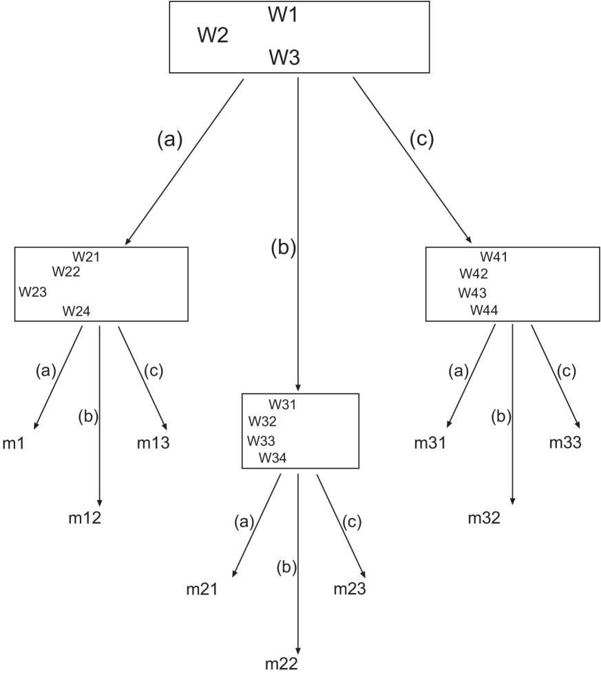
Figure 8: Flowchart showing different asymptotic limits for the “islands” example.

References

- [1] W. Lerche, D. Lüst and A. N. Schellekens, “Chiral Four-Dimensional Heterotic Strings From Selfdual Lattices,” Nucl. Phys. B 287, 477 (1987).
- [2] R. Bousso and J. Polchinski, “Quantization of four-form fluxes and dynamical neutralization of the cosmological constant,” JHEP 0006, 006 (2000) [arXiv:hep-th/0004134].
- [3] M. R. Douglas, “The statistics of string / M theory vacua,” JHEP 0305 046 (2003) [arXiv:hep-th/0303194]; F. Denef and M. R. Douglas, “Distributions of flux vacua,” JHEP 0405, 072 (2004) [arXiv:hep-th/0404116];
- [4] M. R. Douglas and S. Kachru, “Flux compactification,” arXiv:hep-th/0610102; F. Denef, M. R. Douglas and S. Kachru, “Physics of String Flux Compactifications,” arXiv:hep-th/0701050.
- [5] U. H. Danielsson, N. Johansson and M. Larfors, “The world next door: Results in landscape topography,” arXiv:hep-th/0612222.
- [6] S. Kachru, R. Kallosh, A. Linde and S. P. Trivedi, “De Sitter vacua in string theory,” Phys. Rev. D 68, 046005 (2003) [arXiv:hep-th/0301240].
- [7] A.D. Linde, Particle Physics and Inflationary Cosmology (Harwood, Chur, Switzerland, 1990) [arXiv:hep-th/0503203].
- [8] A. D. Linde, D. A. Linde and A. Mezhlumian, “From the Big Bang theory to the theory of a stationary universe,” Phys. Rev. D 49, 1783 (1994) [arXiv:gr-qc/9306035].
- [9] A. Vilenkin, “The Birth Of Inflationary Universes,” Phys. Rev. D 27, 2848 (1983).
- [10] A. D. Linde, Eternally Existing Self-reproducing Chaotic Inflationary Universe,” Phys. Lett. B 175, 395 (1986).
- [11] L. Susskind, “The anthropic landscape of string theory,” arXiv:hep-th/0302219.
- [12] J. Garcia-Bellido, A. D. Linde and D. A. Linde, “Fluctuations of the gravitational constant in the inflationary Brans-Dicke cosmology,” Phys. Rev. D 50, 730 (1994) [arXiv:astro-ph/9312039]; J. Garcia-Bellido and A. D. Linde, “Stationarity of inflation and predictions of quantum cosmology,” Phys. Rev. D 51, 429 (1995) [arXiv:hep-th/9408023]; J. Garcia-Bellido and A. D. Linde, “Stationary solutions in Brans-Dicke stochastic inflationary cosmology,” Phys. Rev. D 52, 6730 (1995) [arXiv:gr-qc/9504022].
- [13] A. Vilenkin, “Predictions from quantum cosmology,” Phys. Rev. Lett. 74, 846 (1995) [arXiv:gr-qc/9406010].
- [14] A. Vilenkin, “Making predictions in eternally inflating universe,” Phys. Rev. D 52, 3365 (1995) [arXiv:gr-qc/9505031]; S. Winitzki and A. Vilenkin, “Uncertainties of predictions in models of eternal inflation,” Phys. Rev. D 53, 4298 (1996) [arXiv:gr-qc/9510054]; J. Garriga and A. Vilenkin, “A prescription for probabilities in eternal inflation,” Phys. Rev. D 64, 023507 (2001) [arXiv:gr-qc/0102090]; J. Garriga, D. Schwartz-Perlov, A. Vilenkin and S. Winitzki, “Probabilities in the inflationary multiverse,” JCAP 0601, 017 (2006) [arXiv:hep-th/0509184]; R. Easther, E. A. Lim and M. R. Martin, “Counting pockets with world lines in eternal inflation,” JCAP 0603, 016 (2006) [arXiv:astro-ph/0511233]; A. Vilenkin, “Probabilities in the landscape,” arXiv:hep-th/0602264; A. Vilenkin, “Freak observers and the measure of the multiverse,” arXiv:hep-th/0611271; S. Winitzki, “Predictions in eternal inflation,” arXiv:gr-qc/0612164; V. Vanchurin, “Geodesic measures of the landscape,” arXiv:hep-th/0612215.
- [15] A. D. Linde and A. Mezhlumian, “On Regularization Scheme Dependence of Predictions in Inflationary Cosmology,” Phys. Rev. D 53, 4267 (1996) [arXiv:gr-qc/9511058].
- [16] M. Tegmark, “What does inflation really predict?,” JCAP 0504, 001 (2005) [arXiv:astro-ph/0410281].
- [17] A. Aguirre, S. Gratton and M. C. Johnson, “Hurdles for recent measures in eternal inflation,” arXiv:hep-th/0611221.
- [18] A. A. Starobinsky, “Stochastic De Sitter (Inflationary) Stage In The Early Universe,” in: Current Topics in Field Theory, Quantum Gravity and Strings, Lecture Notes in Physics, eds. H.J. de Vega and N. Sanchez (Springer, Heidelberg 1986) 206, p. 107.
- [19] A. S. Goncharov, A. D. Linde and V. F. Mukhanov, “The Global Structure Of The Inflationary Universe,” Int. J. Mod. Phys. A 2, 561 (1987).
- [20] J. Garriga, D. Schwartz-Perlov, A. Vilenkin and S. Winitzki, “Probabilities in the inflationary multiverse,” JCAP 0601, 017 (2006) [arXiv:hep-th/0509184].
- [21] R. Bousso, “Holographic probabilities in eternal inflation,” Phys. Rev. Lett. 97, 191302 (2006) [arXiv:hep-th/0605263].
- [22] V. Vachurin, “Geodesic Measures of the Landscape,” arXiv:hep-th/0612215
- [23] S. W. Hawking and T. Hertog, “Populating the landscape: A top down approach,” Phys. Rev. D 73, 123527 (2006) [arXiv:hep-th/0602091].
- [24] J. B. Hartle and S. W. Hawking, “Wave Function Of The Universe,” Phys. Rev. D 28, 2960 (1983).
- [25] A. D. Linde, “Quantum Creation Of The Inflationary Universe,” Lett. Nuovo Cim. 39, 401 (1984); A. Vilenkin, “Quantum Creation Of Universes,” Phys. Rev. D 30, 509 (1984).
- [26] A. Ceresole, G. Dall’Agata, A. Giryavets, R. Kallosh and A. Linde, “Domain walls, near BPS bubbles, and probabilities in the landscape,” Phys. Rev. D 74, 086010 (2006) [arXiv:hep-th/0605266]
- [27] A. Linde, “Sinks in the landscape, Boltzmann Brains, and the cosmological constant problem” arXiv:hep-th/0611043.
- [28] S. R. Coleman and F. De Luccia, “Gravitational Effects On And Of Vacuum Decay,” Phys. Rev. D 21, 3305 (1980).
- [29] A. D. Linde, “Hard art of the universe creation (stochastic approach to tunneling and baby universe formation),” Nucl. Phys. B 372, 421 (1992) [arXiv:hep-th/9110037].
- [30] A. H. Guth and E. J. Weinberg, “Could The Universe Have Recovered From A Slow First Order Phase Transition?,” Nucl. Phys. B 212, 321 (1983).
- [31] S. W. Hawking and I. G. Moss, “Supercooled Phase Transitions In The Very Early Universe,” Phys. Lett. B 110, 35 (1982).
- [32] E. J. Weinberg, “Does the Hawking-Moss bounce calculate a decay rate?,” arXiv:hep-th/0612146.
- [33] U. Gen and M. Sasaki, “False vacuum decay with gravity in non-thin-wall limit,” Phys. Rev. D 61, 103508 (2000) [arXiv:gr-qc/9912096].
- [34] A. S. Goncharov and A. D. Linde, “Tunneling in an Expanding Universe: Euclidean and Hamiltonian Approaches,” Fiz. Elem. Chast. Atom. Yadra 17, 837 (1986) (Sov. J. Part. Nucl. 17, 369 (1986)).
- [35] K. M. Lee and E. J. Weinberg, “Decay Of The True Vacuum In Curved Space-Time,” Phys. Rev. D 36, 1088 (1987).
- [36] J. Garriga and A. Vilenkin, “Recycling universe,” Phys. Rev. D 57, 2230 (1998) [arXiv:astro-ph/9707292].
- [37] A. Aguirre and M. C. Johnson, “Two tunnels to inflation,” Phys. Rev. D 73, 123529 (2006) [arXiv:gr-qc/0512034].
- [38] L. Dyson, M. Kleban and L. Susskind, “Disturbing implications of a cosmological constant,” JHEP 0210, 011 (2002) [arXiv:hep-th/0208013].
- [39] A. D. Linde, “Quantum creation of an open inflationary universe,” Phys. Rev. D 58, 083514 (1998) [arXiv:gr-qc/9802038].
- [40] A. R. Frey, M. Lippert and B. Williams, “The fall of stringy de Sitter,” Phys. Rev. D 68, 046008 (2003) [arXiv:hep-th/0305018].
- [41] D. Green, E. Silverstein and D. Starr, “Attractor explosions and catalyzed vacuum decay,” Phys. Rev. D 74, 024004 (2006) [arXiv:hep-th/0605047].
- [42] U. H. Danielsson, N. Johansson and M. Larfors, “Stability of flux vacua in the presence of charged black holes,” JHEP 0609, 069 (2006) [arXiv:hep-th/0605106].