hep-th/0701070

Entropy of Three-Charge Black Holes on a Circle

Troels Harmark$\,{}^{1}$, Kristjan R. Kristjansson$\,{}^{2}$, Niels A. Obers$\,{}^{1}$, Peter B. Rønne$\,{}^{1}$

¹ The Niels Bohr Institute
Blegdamsvej 17, 2100 Copenhagen Ø, Denmark

² Nordita
Blegdamsvej 17, 2100 Copenhagen Ø, Denmark

harmark@nbi.dk, kristk@nordita.dk, obers@nbi.dk, roenne@nbi.dk

We study phases of five-dimensional three-charge black holes with a circle in their transverse space. In particular, when the black hole is localized on the circle we compute the corrections to the metric and corresponding thermodynamics in the limit of small mass. When taking the near-extremal limit, this gives the corrections to the finite entropy of the extremal three-charge black hole as a function of the energy above extremality. For the partial extremal limit with two charges sent to infinity and one finite we show that the first correction to the entropy is in agreement with the microscopic entropy by taking into account that the number of branes shift as a consequence of the interactions across the transverse circle.

1 Introduction

Three-charge black holes in five dimensions play a prominent role in string theory. In particular, these black holes are the first examples where a microscopic description [1, 2] of the entropy was achieved in terms of degeneracies of D-brane states. These three-charge black holes, and the closely related two-charge systems, continue to provide a fertile ground for further exploration of the microscopic origin of entropy in string theory (see e.g. the review [3]) and, more generally, the AdS₃/CFT₂ correspondence [4].

In this talk, we review recent results [5] on these three-charge systems in the setting where one of the spatial dimensions is compactified on a circle, i.e. when the five-dimensional spacetime is asymptotically $\mathcal{M}^{4}\times S^{1}$. Of special interest here is the case when the black hole is localized on the circle. Considered on the covering space of the circle, this corresponds to an infinite array of black holes on a line, separated by a distance equal to the circumference of the circle. At extremality, it follows from the BPS property that electric repulsion cancels the gravitation attraction, so that the entropy is given by the finite result $S=2\pi\sqrt{N_{1}N_{4}N_{0}}$. However, when we move away from extremality the black holes will start to interact with each other and as a consequence the entropy will receive corrections. Here we summarize how, in the large radius limit, the first two leading corrections of this entropy can be computed by relating five-dimensional three-charge black holes on a circle to neutral Kaluza-Klein black holes (see the reviews [6, 7, 8]) in five dimensions. This map also enables us to numerically obtain the entire phase of three-charge black holes localized on a circle. A more general consequence of the map is the appearance of a rich phase structure for three-charge black holes on a circle, including a new phase where the black holes are non-uniformly smeared on the circle. We also review the non-trivial fact that, when two charges are extremal and one is kept finite, the first correction to the macroscopic entropy obtained for the localized case can be understood from a microstate counting picture.

2 Generating three-charge black holes on a circle

The method we employ to generate the three-charge black holes we are interested in, builds on the technique used in [9], where it was shown that any Kaluza-Klein black hole in $d+1$ dimensions ($4\leq d\leq 9$) can be mapped to a corresponding brane solution of Type IIA/IIB String Theory and M-theory, following the procedure originally conceived in [10]. These are thermal excitations of extremal 1/2-BPS branes in String/M-theory with transverse space $R^{d-1}\times S^{1}$. This gives a precise connection between the rich phase structure of Kaluza-Klein black holes and that of the corresponding brane. In particular, by considering the near-extremal limit of the latter, the thermodynamic behavior of the non-gravitational theories dual to near-extremal branes on a circle is obtained via the map.

By considering the particular case of Kaluza-Klein black holes in five dimensions $(d=4)$, the above map can be generalized to generate non-extremal three-charge brane configurations in Type IIA/IIB String Theory and M-theory from any neutral five-dimensional Kaluza-Klein black hole. We generally work in the duality frame where these charges are carried by the F1-D0-D4 system, and the solutions obtained are thermal excitations of the corresponding extremal 1/8-BPS brane system. When reduced on the spatial world-volume directions of these branes, we then obtain three-charge black holes in five-dimensional supergravity.

There is considerable knowledge on the phase structure of five-dimensional Kaluza-Klein black holes. While there are four known phases, we will confine ourselves to the following three: i) The uniform phase, i.e. the black string which is a four-dimensional Schwarzschild black hole times a circle, so the horizon topology is $S^{2}\times S^{1}$; ii) The non-uniform phase, which is a static solution emerging from the uniform phase at the Gregory-Laflamme point where the black string is marginally unstable. For five dimensions, the leading order behavior of this phase was first found numerically in [13] and recently extended into the non-linear regime in Ref. [14]. This phase also has horizon topology $S^{2}\times S^{1}$ but the horizon is non-uniform along the direction of the circle; iii) The localized phase, which approaches the five-dimensional Schwarzschild black hole in the limit of zero mass. The first correction to this metric in the small-mass limit is known analytically [15] (see also [16]) using the ansatz proposed in [17] and recently also the second correction [18, 19], while the most recent numerical data on the entire phase can be found in Ref. [20]. The horizon topology in this phase is $S^{3}$.

The three-charge solutions that we are interested in can then be generated by using these neutral five-dimensional Kaluza-Klein black holes as seeding solutions. Starting with any such five-dimensional solution we add five flat dimensions and then act on the solution with a series of three boosts and various U-dualities, where each boost adds one charge to the system. The new solution has metric [5]

$$ds_{10}^{2}=H_{1}^{-\frac{3}{4}}H_{4}^{-\frac{3}{8}}H_{0}^{-\frac{7}{8}}\left(-Udt^{2}+H_{4}H_{0}dx^{2}+H_{1}H_{0}\sum_{i=1}^{4}(du^{i})^{2}+H_{1}H_{4}H_{0}\frac{L^{2}}{(2\pi)^{2}}V_{\alpha\beta}dx^{\alpha}dx^{\beta}\right)\ ,$$ (1)

where $U$ and $(L/2\pi)^{2}V_{\alpha\beta}$ ($1\leq\alpha,\beta\leq 4$) are the metric components of the five-dimensional seeding solution. The dilaton and gauge potentials are given by

$$e^{2\phi}=H_{1}^{-1}H_{4}^{-\frac{1}{2}}H_{0}^{\frac{3}{2}},\quad A_{a}=\coth\alpha_{a}(H_{a}^{-1}-1)dt\wedge d\omega_{a},\textrm{ for }a=1,4,0\ ,$$ (2)

where $H_{a}$ are harmonic functions on the transverse space, given by

$$H_{a}=1+(1-U)\sinh^{2}\alpha_{a},\quad\textrm{for }a=1,4,0\ .$$ (3)

This three-charge solution describes a non-extremal configuration with F1-string, D4-brane and D0-brane charges, with the label $a=1,4,0$ referring to the type of object. To compare with the five-dimensional black hole, we can compactify again the five added dimensions.

Each of the three phases of Kaluza-Klein black holes described above thus directly maps onto a corresponding phase of non-extremal three-charge black holes and we can express the thermodynamic properties in terms of those of the seeding solution. For the non-extremal three-charge black holes described above, the physical quantities that we can measure asymptotically are the mass, $\bar{M}$, the three charges $Q_{a}$, and the tension ${\mathcal{T}}$ in the transverse direction. We define dimensionless mass $\bar{\mu}=g\bar{M}$ and charge $q_{a}=gQ_{a}$ using the dimensionfull parameter $g$, defined in Eq. (5), that involves the Newton’s constant, the size of the circle and the volume of the five new additional dimensions that we take to be compactified on a torus. The relative tension is defined as $\bar{n}=L{\mathcal{T}}/(\bar{M}-M^{\textrm{el}})$ [21] where in the denominator we subtract the electric part of the mass from the total mass.

By comparing the asymptotic behavior of the seeding solution to the three-charge solution, we can get a map from $\mu$ and $n$ of the original neutral black hole [22, 23] and the boost parameters $\alpha_{a}$, to the physical quantities of the new charged solution, $\bar{\mu}$, $q_{a}$ and $\bar{n}$. Given the value of the three charges we can write the mass and relative tension of the charged solutions as [5]

$$\bar{\mu}=\sum_{a}q_{a}+\frac{1}{2}\mu n+\frac{(2-n)\mu}{6}\sum_{a}\frac{b_{a}}{1+\sqrt{1+b_{a}^{2}}},\quad b_{a}\equiv\frac{2-n}{6}\frac{\mu}{q_{a}}\;\;\;,\qquad\bar{n}=n\ .$$ (4)

The neutral seeding solution always has $\mu\geq 0$ and $0\leq n\leq 2$ so the last two terms are positive, and therefore we see that for fixed $q_{a}$, the mass $\bar{\mu}$ is bounded from below by the sum of the charges, which is the extremal mass. The energy above extremality will thus be defined as the mass minus the sum of the charges.

3 Near-extremal limit and thermodynamics

The map above becomes especially simple (as was the case for the one-charge branes considered in Ref. [9]) when we take the near-extremal limit. This limit is also relevant for the dual CFT description of these brane systems and for our application to microstate counting. The near-extremal limit we take has the property that the energy above extremality has the same scale as the size of the circle, and is defined as

$$L\to 0,\quad\alpha_{a}\to\infty,\quad\ell_{a}\equiv L^{\gamma_{a}}\sqrt{q_{a}}\textrm{ fixed},\quad g\equiv\frac{16\pi G_{10}}{V_{1}V_{4}L^{2}}\textrm{ fixed}\ .$$ (5)

Here $\gamma_{a}$ are positive constants that sum to one. When one of them is taken to be zero the corresponding charge remains finite in the near-extremal limit. In order to get finite results, we must rescale all background fields with appropriate powers of $L$ and in order for this rescaling to be a symmetry of the action, the 10-dimensional Newton’s constant needs to be rescaled so that $g$ remains fixed.

Taking the limit (5) on the non-extremal three-charge solution (1), (2) produces a new solution of near-extremal three-charge black holes on a circle, in which essentially the constant “1” in the harmonic functions (3) has disappeared (see [5] for details). The asymptotic physical quantities for the near-extremal solution are the energy above extremality $\epsilon=gE$, which is the mass minus the charges, and the tension of the circle $\hat{\mathcal{T}}$. The relative tension is now defined as $r=2\pi\hat{\mathcal{T}}/E$. The map from $(\mu,n)$ of the neutral seeding solution to $(\epsilon,r)$ of the near-extremal three-charge solution turns out to be surprisingly simple [5]

$$\epsilon=\mu n/2,\quad r=2\ .$$ (6)

It is interesting to notice that the relative tension is independent of the parameters of the original black hole. This means that the three phases all collapse on top of each other in the $(\epsilon,r)$ diagram. This result is intimately related to the finite non-vanishing entropy in the extremal limit [5]. Furthermore, given the rescaled entropy ${\mathfrak{s}}$ and temperature ${\mathfrak{t}}$ of the seeding solution, we can find the rescaled entropy $\hat{\mathfrak{s}}$ and temperature $\hat{\mathfrak{t}}$ of the near-extremal solution via the map [5]

$$\hat{\mathfrak{t}}={\mathfrak{t}}({\mathfrak{t}}{\mathfrak{s}})^{3/2},\quad\hat{\mathfrak{s}}={\mathfrak{s}}({\mathfrak{t}}{\mathfrak{s}})^{-3/2}\ .$$ (7)

Reinstating the units for the rescaled entropy we obtain the relation $S=\hat{\mathfrak{s}}\ 2\pi\sqrt{N_{1}N_{4}N_{0}}$ where $N_{a}$, $a=1,4,0$ are the number of each type of extended object in the system.

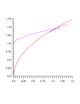
Figure 1: The entropy $\hat{\mathfrak{s}}=S/(2\pi\sqrt{N_{1}N_{4}N_{0}})$ as a function of the energy above extremality $\epsilon$ for the localized phase (magenta), the uniform phase (red) and the non-uniform phase (blue). The curves for the localized/non-uniform phase are based on the numerical data of [20] and [14] respectively. We see that the localized phase starts out at finite entropy. It has higher entropy than the uniform phase and is therefore thermodynamically stable. At some point the curves of the localized and the uniform phases meet and the non-uniform phase interpolates between them.

We can now apply the map to the known thermodynamics of each of the three phases for the neutral seeding solution, and obtain the thermodynamics of the corresponding three phases of three-charge black holes. As an example, Fig. 1 shows the entropy as a function of energy in the near-extremal case for each of these three different phases, using numerical data of Ref. [20, 14]. Moreover, from analytic results for small localized Kaluza-Klein black holes [15, 16, 18, 19] we get an expansion for the entropy of localized near-extremal three-charge black holes on a circle [5]

$$S=2\pi\sqrt{N_{1}N_{4}N_{0}}\left(1+\sqrt{\frac{\epsilon}{8}}+\frac{\epsilon}{16}+{\mathcal{O}}(\epsilon^{3/2})\right)\ .$$ (8)

This central result presents the first two corrections to the finite extremal entropy [1], in a small energy (or equivalently, large circle radius) expansion.

We can also consider other near-extremal limits, for example keeping one of the three charges finite while sending the other two to infinity, by taking one of the $\gamma_{a}$ in (5) to be zero. Choosing $\gamma_{0}=0$, corresponding to keeping finite D0-brane charge, we then find for the localized black hole the energy above extremality and entropy [5]

$$\epsilon =\rho_{0}^{2}\sinh^{2}\alpha_{0}+\frac{1}{2}\rho_{0}^{2}\left(1+\frac{1}{16}\rho_{0}^{2}\right)+{\cal{O}}(\rho_{0}^{6})\ ,$$ (9)

$$\hat{\mathfrak{s}} =\rho_{0}\cosh\alpha_{0}\left(1+\frac{1}{16}\rho_{0}^{2}+\frac{1}{512}\rho_{0}^{4}\right)+{\mathcal{O}}(\rho_{0}^{7})\ .$$ (10)

Here $\rho_{0}$ is a small parameter of the original seeding solution, related to the location of the event horizon and thus controlling the size of the neutral black hole relative to the circle radius. In the next section we will review how the expression for the entropy can be reproduced from a microstate counting point of view.

4 Microscopic counting of entropy

We now want to recalculate the entropy using microstate counting techniques. First, we recall how the microstate entropy formula is generalized to non-extremal black holes that are not on a circle. In the weak coupling limit, the extremal black hole can be described as a configuration with $N_{4}$ D4-branes, a number $N_{1}$ of fundamental strings stretching between the D4-branes and $N_{0}$ D0-branes that are threaded on the fundamental strings [1]. Non-extremal black holes can be generated by, for example, adding a number $N_{\bar{0}}$ of anti-D0-branes. Horowitz, Maldacena and Strominger [24] argued that in the dilute gas limit, the forces between the D0- and anti-D0-branes would be very small and interactions could be ignored. The entropy is thus given by the sum of the square-roots [24]

$$S=2\pi\sqrt{N_{1}N_{4}}\left(\sqrt{N_{0}}+\sqrt{N_{\bar{0}}}\right)\ .$$ (11)

This is the formula that we want to generalize to our three-charge black holes on a circle. In the non-extremal formula the D0- and anti-D0-branes were far apart and did not interact, but with the small transverse circle present, that is no longer a safe assumption to make. In our near-extremal limit (5), the size of the transverse circle is taken to be at the same scale as the energy above extremality and the interaction energy is therefore not negligible compared to the excitation energy. That means that interactions of the zero-branes across the circle must be taken into account. The effect of the interaction is to shift the number of D0-branes for a given total energy [25]. To find the entropy we must therefore find the effective number of branes $N_{0}^{\prime}$ and $N_{\bar{0}}^{\prime}$.

To this end we write the total mass of our three-charge system as

$$\bar{M}=Q_{1}+Q_{4}+\delta E+V_{\textrm{int}}\ ,$$ (12)

where $\delta E$ is the energy carried by the D0-branes and the anti-D0-branes, and $V_{\textrm{int}}$ is the interaction energy related to the presence of the transverse circle. As we start adding anti-D0-branes to the extremal system, they will interact with the D0-branes across the circle, reducing their energy by $V_{\textrm{int}}={\mathcal{T}}L/2$. We find the effective number of D0- and anti-D0-branes from requiring

$$\delta E\simeq N^{\prime}_{0}+N^{\prime}_{\bar{0}},\quad Q_{0}\simeq N^{\prime}_{0}-N^{\prime}_{\bar{0}}\ .$$ (13)

Applying this method to the localized phase of the three-charge black hole on a circle and inserting the effective numbers into Eq. (11) we obtain the entropy

$$S=\frac{2\pi\sqrt{N_{1}N_{4}N_{0}}}{\ell_{0}}\rho_{0}\cosh\alpha_{0}\left(1+\frac{\rho_{0}^{2}}{16}+\mathcal{O}(\rho_{0}^{4})\right).$$ (14)

We hence find that the leading order correction of this microscopic entropy is in agreement with the leading order correction of the macroscopic entropy in (9).

5 Conclusion

We have shown how to generate five-dimensional three-charge black hole solutions on a circle, from known phases of five-dimensional Kaluza-Klein black holes and considered the near-extremal limit of these. In particular, we have computed the first corrections to the finite entropy of (extremal) localized three-charge black holes and matched, in a partial near-extremal limit, the macroscopic entropy with a microscopic calculation. We believe this is a non-trivial check on the microscopic picture employed here, while at the same time illustrating the power of the map. We have also obtained an entirely new phase of non- and near-extremal three-charges black holes, which are non-uniformly distributed along the circle.

One open direction is to further examine the microscopic description of these black holes. In this connection, the entropy matching discussed here was recently extended to second order in Ref. [26]. Furthermore, in Ref. [26] a simple microscopic model was proposed that reproduces most of the features of the phase diagram, including the new non-uniform phase. The study of other new three-charge solutions, arising from bubble-black hole sequences will also be interesting and we intend to report on this in the future [12]. Finally, further examination of the non-uniform phase of three-charge black holes and the classical stability of the uniform phase along the lines of [27], and its relation to correlated stability conjecture would be interesting to pursue.

References

- [1] A. Strominger and C. Vafa, Phys. Lett. B379 (1996) 99–104, hep-th/9601029.
- [2] J. Curtis G. Callan and J. M. Maldacena, Nucl. Phys. B472 (1996) 591–610, hep-th/9602043.
- [3] S. D. Mathur, Class. Quant. Grav. 23 (2006) R115, hep-th/0510180.
- [4] J. Maldacena, Adv. Theor. Math. Phys. 2 (1998) 231–252, hep-th/9711200.
- [5] T. Harmark, K. R. Kristjansson, N. A. Obers, and P. B. Ronne, JHEP 01 (2007) 023, hep-th/0606246.
- [6] T. Harmark and N. A. Obers, hep-th/0503020.
- [7] B. Kol, Phys. Rept. 422 (2006) 119–165, hep-th/0411240.
- [8] T. Harmark, V. Niarchos, and N. A. Obers, hep-th/0701022. To appear in Class. Quant. Grav.
- [9] T. Harmark and N. A. Obers, JHEP 09 (2004) 022, hep-th/0407094.
- [10] S. F. Hassan and A. Sen, Nucl. Phys. B375 (1992) 103–118, hep-th/9109038.
- [11] H. Elvang, T. Harmark, and N. A. Obers, JHEP 01 (2005) 003, hep-th/0407050.
- [12] T. Harmark, K. R. Kristjansson, N. A. Obers, and P. B. Ronne, Work in progress.
- [13] S. S. Gubser, Class. Quant. Grav. 19 (2002) 4825–4844, hep-th/0110193.
- [14] B. Kleihaus, J. Kunz, and E. Radu, JHEP 06 (2006) 016, hep-th/0603119.
- [15] T. Harmark, Phys. Rev. D69 (2004) 104015, hep-th/0310259.
- [16] D. Gorbonos and B. Kol, Class. Quant. Grav. 22 (2005) 3935–3960, hep-th/0505009.
- [17] T. Harmark and N. A. Obers, JHEP 05 (2002) 032, hep-th/0204047.
- [18] D. Karasik, C. Sahabandu, P. Suranyi, and L. C. R. Wijewardhana, Phys. Rev. D71 (2005) 024024, hep-th/0410078.
- [19] Y.-Z. Chu, W. D. Goldberger, and I. Z. Rothstein, JHEP 03 (2006) 013, hep-th/0602016.
- [20] H. Kudoh and T. Wiseman, Phys. Rev. Lett. 94 (2005) 161102, hep-th/0409111.
- [21] T. Harmark and N. A. Obers, JHEP 05 (2004) 043, hep-th/0403103.
- [22] T. Harmark and N. A. Obers, Class. Quantum Grav. 21 (2004) 1709–1724, hep-th/0309116.
- [23] B. Kol, E. Sorkin, and T. Piran, Phys. Rev. D69 (2004) 064031, hep-th/0309190.
- [24] G. T. Horowitz, J. M. Maldacena, and A. Strominger, Phys. Lett. B383 (1996) 151–159, hep-th/9603109.
- [25] M. S. Costa and M. J. Perry, Nucl. Phys. B591 (2000) 469–487, hep-th/0008106.
- [26] B. D. Chowdhury, S. Giusto, and S. D. Mathur, hep-th/0610069.
- [27] T. Harmark, V. Niarchos, and N. A. Obers, JHEP 10 (2005) 045, hep-th/0509011.