Giant Gravitons - with Strings Attached (I)

Robert de Mello Koch1,2, Jelena Smolic1 and Milena Smolic1
  
1Department of Physics and Centre for Theoretical Physics,
University of the Witwatersrand,
Wits, 2050,
South Africa
  
2Stellenbosch Institute for Advanced Studies,
Stellenbosch,
South Africa
  
E-mail
robert@neo.phys.wits.ac.za, smolicj@science.pg.wits.ac.za, smolicm@science.pg.wits.ac.za
Abstract:

In this article, the free field theory limit of operators dual to giant gravitons with open strings attached, are studied. We introduce a graphical notation, which employs Young diagrams, for these operators. The computation of two point correlation functions is reduced to the application of three simple rules, written as graphical operations performed on the Young diagram labels of the operators. Using this technology, we have studied gravitational radiation by giant gravitons and bound states of giant gravitons, transitions between excited giant graviton states and joining of open strings attached to the giant.

Giant Gravitons, AdS/CFT correspondence, super Yang-Mills theory
preprint: WITS-CTP-031

1 Introduction

The gauge theory/gravity correspondence[1],[2],[3] has provided deep and unexpected links between string theory on negatively curved spacetime, large $N$ quantum field theories and spin chains. For example, according to the correspondence, the masses of states in the string theory coincide with anomalous dimensions of operators in the field theory. These anomalous dimensions are also given by the spectrum of a spin chain. In this article we will study the original example of the correspondence, which relates ${\cal N}=4$ super Yang-Mills theory to type IIB string theory on the AdS${}_{5}\times$S5 background.

The correspondence is a strong/weak coupling duality in the ’t Hooft coupling of the field theory. Therefore, computations that can be carried out on both sides of the correspondence necessarily compute quantities that are not corrected or receive small corrections, allowing weak coupling results to be extrapolated to strong coupling. As an example, an interesting set of observables to consider are dual to single graviton perturbations of AdS${}_{5}\times$S5. These perturbations are members of a BPS multiplet so that their energies are protected by supersymmetry. For these observables, one could also test that AdS/CFT reproduces the correct field theory correlation functions.

Part of the difficulty in understanding the AdS/CFT correspondence is related to the fact that we do not as yet have a good understanding of how to quantize the superstring in this background. There are however, interesting geometric limits where the string can be quantized exactly[4]. On the field theory side, one takes a different large $N$ limit - the energy and ${\cal R}$-charges of the observables are also scaled in the new limit[5]. The result is a systematic way to relax the supersymmetry enjoyed by a state. The operators which one obtains (BMN loops) are nearly supersymmetric, and consequently although they are corrected, the perturbation theory is suppressed by the large quantum numbers of the states in question. This allowed the use of perturbation theory to explore the strong coupling regime of the gauge theory and consequently, truly stringy aspects of the AdS/CFT correspondence could be probed.

The single graviton observables could be studied, on the gravity side of the correspondence, using a supergravity approximation. The states dual to BMN loops could be studied within the framework of perturbative string theory in the pp-wave limit. However, we should be able to do even more. The AdS/CFT correspondence is a non-perturbative equivalence, and hence should also allow one to understand non perturbative objects in string theory on the AdS geometry. Since we only have control over the weakly coupled limit of the field theory, we still want to study objects that are protected. Giant gravitons are good examples of protected non perturbative objects. Indeed, since they are half-BPS states, giant gravitons have proved to be the source of many valuable quantities that are accessible on both sides of the correspondence.

Giant graviton solutions describe branes extended in the sphere[6] or in the AdS space [7],[8],[9] of the AdS$\times$S background. The giant gravitons are (classically) stable due to the presence of the five form flux which produces a force that exactly balances their tension. The dual description of giant gravitons in the Yang-Mills theory has enjoyed some progress. Operators dual to giant gravitons (Schur polynomials in the Higgs fields) have been proposed in [10],[11]. However, despite compelling evidence (reviewed in section 2.1) for the identification of Schur polynomials as the operators dual to giant gravitons, a detailed understanding of this correspondence has not yet been achieved. For example, even a basic understanding of how the geometry of the giant graviton is coded in the dual operator, is not complete.

Excitations of giant gravitons can be obtained by attaching open strings to the giants. The gauge theory operators dual to excited sphere giants are known and their anomalous dimensions reproduce the expected open string spectrum[12]111See [13],[14],[15] for further studies of non-BPS excitations that have been interpreted as open strings attached to giant gravitons.. Recently, operators dual to an arbitrary system of excited giant gravitons have been proposed in the insightful paper[16]. The proposal has been tested by showing that the restrictions imposed on excitations of the system, by the Gauss law, are indeed satisfied. For the general case, it is an involved combinatoric task to compute the two point functions of these operators (even in the free field limit) and further to compute their anomalous dimensions. Our goal in this article is to start developing the required technology.

The study of excitations of giant gravitons is likely to shed light on the precise details of the Schur polynomial/giant graviton correspondence, which is one of the main motivations for our study. Concretely, we study two point functions in the free theory, of operators dual to excited giant graviton systems. With a specific choice for the open string excitations, we can factorize the problem of computing correlators into a factor involving only the open string words and a factor involving the Schur polynomial itself. The factor involving the open string words can be dealt with using the usual ${1\over N}$ expansion. The factor involving the Schur polynomial contains $O(N)$ fields, so that huge combinatoric factors over power the usual ${1\over N^{2}}$ suppression of non-planar diagrams and new techniques for evaluating these factors are needed. We develop the required technology. Our result is a set of simple geometrical operations performed on the Young diagram labeling the operator, allowing an efficient computation of the factor involving the Schur polynomials. In this article we deal with the free field theory. However, it is possible to extend our rules, providing efficient methods that allow the computation of the leading $g_{YM}^{2}$ correction coming from the $F$-terms. This is reported in a separate paper[17].

The world volume theory of giant gravitons at low energy is a Yang-Mills theory. Since the world volume of the giant gravitons does not coincide with the spacetime on which the original Yang-Mills theory is defined, this new Yang-Mills theory (which “emerges” from the original one) will be local in a new space[16], which arises from the matrix degrees of freedom of the original field theory. Our main application for the methods developed in this article, is to explore this emergent Yang-Mills theory. In particular, we have studied gravitational radiation by giant gravitons and bound states of giant gravitons, transitions between excited giant graviton states and the joining and splitting of open strings attached to the giant. The results of our study seem to be consistent with an emergent gauge theory.

Our article is organized as follows: In section 2 we start by reviewing the Schur polynomial/giant graviton correspondence. We then introduce the operators which are conjectured to be dual to excited giant gravitons. Section 2 concludes by summarizing three graphical rules which allow the computation of two point correlators. The technical details of the derivation of the rules are summarized in the appendices. These technical details are not needed to master the rules, which are presented (together with examples) in sections 2.5 and 2.6. A reader wishing only to use our results, need not read more than sections 2.2, 2.3, 2.4 and 2.5. Since the computations involved are rather technical, we have taken the quality assurance of our methods seriously. Towards this end, we have written a MATLAB code which numerically evaluates the correlation functions we study. In appendix J some of these numerical results are summarized. We have verified that our methods correctly reproduce all correlators corresponding to Young diagrams with 5 boxes or less and with two or fewer strings attached.

Section 3 summarizes applications of our methods. In section 3.1 we study gravitational radiation in a number of different settings. This allows us to probe locality in the bulk and also the non-Abelian symmetry of the emergent gauge theory. In section 3.2 we consider transitions between excited giant graviton states. In section 3.3 we study the splitting and joining of open strings attached to the giant graviton. The results of this section seem to be consistent with a $3+1$ dimensional emergent gauge theory. Section 4 is used to discuss our results.

2 The Dual of Excited Giant Gravitons

In this section the operators we study are defined. In the free field limit there is a simple factorization of the spacetime dependence and the factor arising from the color combinatorics[18]. The spacetime dependence is trivial and consequently, uninteresting. For this reason, we drop all spacetime dependence and focus on the color combinatorics. This amounts to working in zero dimensions. The reader interested in a summary of our main results should consult section 2.2 for the definition of the operators we study and section 2.5 for a summary of our technology.

We study the Lorentzian ${\cal N}=4$ super Yang-Mills theory on $R\times S^{3}$. The advantage of taking this approach is simply that $1/2$-BPS states (and systematically small deformations of these states) of the theory on $R\times S^{3}$ can be described in the s-wave reduction of the Yang-Mills theory, i.e. in a matrix quantum mechanics [19]. According to the state-operator correspondence of conformal field theory, the generator associated to dilations on $R^{4}$ becomes the Hamiltonian for the theory on $R\times S^{3}$. The action of ${\cal N}=4$ super Yang-Mills theory on $R\times S^{3}$ is

$$S={N\over 4\pi\lambda}\int dt\int_{S^{3}}{d\Omega_{3}\over 2\pi^{2}}\left({1\over 2}(D\phi^{i})(D\phi^{i})+{1\over 4}\big{(}\big{[}\phi^{i},\phi^{j}\big{]}\big{)}^{2}-{1\over 2}\phi^{i}\phi^{i}\right),$$

where $\lambda=g_{YM}^{2}N$ is the ’t Hooft coupling and $i,j=1,...,6$. We have not displayed the fermion or the gauge kinetic terms in the action; in this article we only consider the scalar fields. The mass term arises from conformal coupling to the metric of $S^{3}$. We group the six real scalars into three complex fields as follows

$$Z=\phi^{1}+i\phi^{2},\qquad Y=\phi^{3}+i\phi^{4},\qquad X=\phi^{5}+i\phi^{6}.$$

In what follows we will use these complex combinations. The free field theory propagators we use are

$$\langle Z^{\dagger}_{ij}(t)Z_{kl}(t)\rangle=\delta_{il}\delta_{jk}=\langle Y^{\dagger}_{ij}(t)Y_{kl}(t)\rangle.$$

We should have a factor of ${4\pi\lambda\over N}$ multiplying the propagator. We have dropped this factor, which clutters formulas and can easily be reinserted at the end of the computation; it contributes an overall factor of $\left({4\pi\lambda\over N}\right)^{m}$, where $m$ is the total number of contractions performed in computing the correlator.

2.1 Giants

There are a number of important clues that can be used to identify the operators dual to giant gravitons. We will study a class of half BPS giant gravitons. The half BPS chiral primary operators we focus on can be built from a single complex combination (we use $Z$ in what follows) of any two of the six Higgs fields appearing in the ${\cal N}=4$ super Yang-Mills theory. Using a total of $n$ $Z$s, there is a distinct operator for each partition of $n$. There is a one to one correspondence between these operators and half BPS representations of R charge $n$[10]. For $n=O(1)$ these half BPS operators are dual to point like gravitons[3], for $n=O(\sqrt{N})$ they are dual to strings[5] and for $n=O(N)$ they are dual to giant gravitons[6]. For the case that $n=O(1)$, operators composed of a product of a different number traces are orthogonal. This naturally allows one to identify the number of traces with particle number and consequently, the supergravity Fock space is clearly visible in the dual gauge theory. For $n=O(N)$, the usual suppression of non-planar diagrams is compensated by combinatoric factors, so that operators composed of a product of a different number of traces, are no longer orthogonal. Clearly then, giant gravitons are not simply dual to operators with a fixed number of traces. One needs a new basis in which the two point functions are again diagonal.

Corley, Jevicki and Ramgoolam have developed a powerful machinery for the exact computation of correlators of Schur polynomials in the zero coupling limit of ${\cal N}=4$ super Yang-Mills theory with gauge group $U(N)$[10]. Their results show that the two point function is diagonalized by the Schur polynomials. It is thus tempting to identify Schur polynomials as the operators dual to giant gravitons[10].

The Schur polynomial is defined by

$$\chi_{R}(Z)={1\over n!}\sum_{\sigma\in S_{n}}\chi_{R}(\sigma)\mbox{Tr\,}(\sigma Z^{\otimes n}),$$ (1)
$$\mbox{Tr\,}(\sigma Z^{\otimes n})=Z^{i_{1}}_{i_{\sigma(1)}}Z^{i_{2}}_{i_{\sigma(2)}}\cdots Z^{i_{n-1}}_{i_{\sigma(n-1)}}Z^{i_{n}}_{i_{\sigma(n)}}.$$

The Schur polynomial label $R$ can be thought of as a Young diagram which has $n$ boxes. $\chi_{R}(\sigma)$ is the character of $\sigma\in S_{n}$ in representation $R$. These operators have conformal dimension $\Delta=n$ and ${\cal R}$ charge $J=n$ and transform in the $(0,n,0)$ of the $SU(4)$ ${\cal R}$ symmetry group. Of course, $\Delta=J$ as expected for a half BPS operator. To state the known results for correlators of Schur polynomials, we need to recall the definition of the weight of a box in a Young diagram. For a box in the $i^{th}$ row and the $j^{th}$ column the weight is $N-i+j$. Let $f_{R}$ denote the product of weights in the Young diagram. For example, if

R1=                          R2=              ,formulae-sequencesubscript𝑅1                          subscript𝑅2              R_{1}=\hbox{}{\vbox{\offinterlineskip\vbox{\hrule height=0.3pt\hbox{\vrule height=6.14993pt,width=0.3pt,depth=2.73328pt\hbox to6.83331pt{\hfil}\vrule height=6.14993pt,width=0.3pt,depth=2.73328pt\hbox to6.83331pt{\hfil}\vrule height=6.14993pt,width=0.3pt,depth=2.73328pt} \hrule height=0.3pt}\vspace{-\y@linethick} \vbox{\hrule height=0.3pt\hbox{\vrule height=6.14993pt,width=0.3pt,depth=2.73328pt\hbox to6.83331pt{\hfil}\vrule height=6.14993pt,width=0.3pt,depth=2.73328pt\hbox to6.83331pt{\hfil}\vrule height=6.14993pt,width=0.3pt,depth=2.73328pt} \hrule height=0.3pt}\vspace{-\y@linethick} \vbox{\hrule height=0.3pt\hbox{\vrule height=6.14993pt,width=0.3pt,depth=2.73328pt\hbox to6.83331pt{\hfil}\vrule height=6.14993pt,width=0.3pt,depth=2.73328pt} \hrule height=0.3pt}\vspace{-\y@linethick} }}\qquad R_{2}=\hbox{}{\vbox{\offinterlineskip\vbox{\hrule height=0.3pt\hbox{\vrule height=6.14993pt,width=0.3pt,depth=2.73328pt\hbox to6.83331pt{\hfil}\vrule height=6.14993pt,width=0.3pt,depth=2.73328pt\hbox to6.83331pt{\hfil}\vrule height=6.14993pt,width=0.3pt,depth=2.73328pt\hbox to6.83331pt{\hfil}\vrule height=6.14993pt,width=0.3pt,depth=2.73328pt\hbox to6.83331pt{\hfil}\vrule height=6.14993pt,width=0.3pt,depth=2.73328pt} \hrule height=0.3pt}\vspace{-\y@linethick} }},

we have

$$f_{R_{1}}=N(N+1)(N-1)N(N-2),\qquad f_{R_{2}}=N(N+1)(N+2)(N+3).$$

The two and three point functions of Schur polynomials, which we use extensively in what follows, are[10]

$$\langle\chi_{R}(Z)\chi_{S}(Z^{\dagger})\rangle=\delta_{RS}f_{R},$$
$$\langle\chi_{R}(Z)\chi_{S}(Z)\chi_{T}(Z^{\dagger})\rangle=g(R,S;T)f_{T},$$

where $g(R,S;T)$ is the Littlewood-Richardson coefficient. For an impressive development of the technology for Schur Polynomials of the $U(N)$ theory, see[20]. For an extension to the $SU(N)$ theory see [20],[21].

Besides the fact that these operators are half BPS and diagonalize the two point function, they capture further features of giant graviton dynamics. To see this, recall that a giant graviton expands to a radius proportional to the square root of its angular momentum[6]. If the giant is expanding in the S5 of the AdS$\times$S background, there is a limit on how large it can be - its radius must be less than the radius of the S5[6]. This in turn implies a cut off on the angular momentum of the giant. Since angular momentum of the giant maps into ${\cal R}$ charge, there should be a cut off on the ${\cal R}$ charge of the dual operators. The Schur polynomials corresponding to totally antisymmetric representations do have a cut off on their ${\cal R}$ charge; this cut off exactly matches the cut off on the giants angular momentum[11]. Thus, it is natural to identify Schur polynomials for the completely antisymmetric representations as the operator dual to sphere giant gravitons. Another class of Schur polynomials which are naturally singled out, are those corresponding to totally symmetric representations. Since these representations are not cut off, they are naturally identified as operators dual to AdS giant gravitons[10], which, because they can expand in the AdS space, can expand to an arbitrarily large size and hence have no bound on their angular momentum. The Young diagram has at most $N$ rows, implying a cut off on the number of AdS giant gravitons; the need for this cut off is clearly visible in the dual gravitational theory: it ensures that the five form flux at the center of the AdS space does not become zero; a non-zero flux is needed to support an AdS giant. To obtain further support for these identifications, one can define a limit in which the dynamics of this half BPS sector decouples from the rest of the theory[19], leading to a description of the half-BPS states in terms of the eigenvalues of large $N$ gauged quantum mechanics for a single Hermitian matrix with quadratic potential. This quantum mechanics is the quantum mechanics of $N$ free non-relativistic fermions in an external potential[22]. The Schur polynomials map into energy eigenfunctions of the $N$ fermion system[10],[19]. Recently, for arbitrary configurations of D-branes which preserve half of the supersymmetries, the full back reaction of the geometry in the supergravity limit was obtained[23]. The phase space structure of non-interacting fermions plays a visible role in these solutions, providing further convincing support for the proposal of [10],[19].

A number of interesting studies exploiting these ideas have appeared recently. For an attempt to recover gravitational thermodynamics see [24]; for an attempt to understand spacetime as an emergent phenomenon see[25]. For a tantalizing suggestion of how to construct the metric of the ${1\over 2}$ BPS geometries directly in the ${\cal N}=4$ super Yang-Mills theory, see [26]. The recent work [27] suggests that many of the results that have been obtained for ${1\over 2}$-BPS giants may have an interesting extension to the ${1\over 4}$ and ${1\over 8}$-BPS cases. For giants in a less supersymmetric background, that may also have a simple field theory dual see[28].

2.2 Excited Giants

As reviewed above, there is significant evidence for the proposal of Corley, Jevicki and Ramgoolam that the dual of a giant graviton is a Schur polynomial. The precise relation between Schur polynomials and giant gravitons however remains obscure. The Schur polynomial corresponding to a Young diagram with one column, with of order $N$ boxes, is naturally interpreted as a sphere giant graviton. Presumably, a Schur polynomial corresponding to a Young diagram with $O(1)$ columns, each with $O(N)$ boxes, corresponds to a bound state of sphere giant gravitons. Similarly, a Schur polynomial corresponding to a Young diagram with $O(1)$ rows, each containing $O(N)$ boxes, is presumably dual to a bound state of AdS giant gravitons. The results of [24] support this interpretation. However, to firmly establish (and define) the precise relation between Schur polynomials and giant gravitons, more detailed computations are required. It is with this goal in mind, that we study excited giant gravitons. Excitations of giant gravitons can be described by attaching open strings to the giant graviton. The open string ends on the giant graviton and so it is natural to suspect that the open string knows something about the giant graviton’s geometry. In this subsection we will describe an attractive proposal for the operators dual to excited giant gravitons[16].

The proposal of [16] amounts, roughly, to inserting words $(W^{(a)})^{j}_{i}$ describing the open strings (one word for each open string) into the operator describing the system of giant gravitons

$$\chi_{R,R_{1}}^{(k)}(Z,W^{(1)},...,W^{(k)})={1\over(n-k)!}\sum_{\sigma\in S_{n}}\mbox{Tr\,}_{R_{1}}(\Gamma_{R}(\sigma))\mbox{Tr\,}(\sigma Z^{\otimes n-k}W^{(1)}\cdots W^{(k)}),$$ (2)
$$\mbox{Tr\,}(\sigma Z^{\otimes n-k}W^{(1)}\cdots W^{(k)})=Z^{i_{1}}_{i_{\sigma(1)}}Z^{i_{2}}_{i_{\sigma(2)}}\cdots Z^{i_{n-k}}_{i_{\sigma(n-k)}}(W^{(1)})^{i_{n-k+1}}_{i_{\sigma(n-k+1)}}\cdots(W^{(k)})^{i_{n}}_{i_{\sigma(n)}}.$$

The representation $R$ of the giant graviton system is a Young diagram with $n$ boxes, i.e. it is a representation of $S_{n}$. $\Gamma_{R}(\sigma)$ is the matrix representing $\sigma$ in irreducible representation $R$ of the symmetric group $S_{n}$. The representation $R_{1}$ is a Young Diagram with $n-k$ boxes, i.e. it is a representation of $S_{n-k}$. Imagine that the $k$ words above are all distinct, corresponding to the case that the open strings are distinguishable. Consider an $S_{n-k}\otimes(S_{1})^{k}$ subgroup of $S_{n}$. The representation $R$ of $S_{n}$ will subduce into a (generically) reducible representation of the $S_{n-k}\otimes(S_{1})^{k}$ subgroup. One of the irreducible representations appearing in this subduced representation is $R_{1}$. $\mbox{Tr\,}_{R_{1}}$ is an instruction to trace only over the indices belonging to this irreducible component. If the representation $R_{1}$ appears more than once, things are a little more subtle. The example discussed in [16] illustrates this point nicely. Suppose $R\to R_{1}\oplus R_{2}\oplus R_{2}$ under restricting $S_{n}$ to $S_{n-2}\times S_{1}\times S_{1}$. Choose a basis so that

$$\Gamma_{R}(\sigma)=\left[\matrix{\Gamma_{R_{1}}(\sigma)_{i_{1}j_{1}}&0&0\cr 0&\Gamma_{R_{2}}(\sigma)_{i_{2}j_{2}}&0\cr 0&0&\Gamma_{R_{2}}(\sigma)_{i_{3}j_{3}}}\right],\qquad\forall\sigma\in S_{n-2}\times S_{1}\times S_{1}.$$

A generic element of $S_{n}$ need not belong to the $S_{n-2}\times S_{1}\times S_{1}$ subgroup and hence need not be block diagonal

$$\Gamma_{R}(\sigma)=\left[\matrix{A^{(1,1)}_{i_{1}j_{1}}&A^{(1,2)}_{i_{1}j_{2}}&A^{(1,3)}_{i_{1}j_{3}}\cr A^{(2,1)}_{i_{2}j_{1}}&A^{(2,2)}_{i_{2}j_{2}}&A^{(2,3)}_{i_{2}j_{3}}\cr A^{(3,1)}_{i_{3}j_{1}}&A^{(3,2)}_{i_{3}j_{2}}&A^{(3,3)}_{i_{3}j_{3}}}\right],\qquad\sigma\notin S_{n-2}\times S_{1}\times S_{1}.$$

There are four suitable definitions for $\mbox{Tr\,}_{R_{2}}(\Gamma_{R}(\sigma))$: $\mbox{Tr\,}(A^{(2,2)})$, $\mbox{Tr\,}(A^{(2,3)})$, $\mbox{Tr\,}(A^{(3,2)})$ or $\mbox{Tr\,}(A^{(3,3)})$. It is natural to interpret the operator obtained using $\mbox{Tr\,}(A^{(2,3)})$ or $\mbox{Tr\,}(A^{(3,2)})$ as dual to the system with the open strings stretching between the giants and the operator obtained using $\mbox{Tr\,}(A^{(2,2)})$ or $\mbox{Tr\,}(A^{(3,3)})$ as dual to the system with one open string on each giant. In general, it is natural to identify the “on the diagonal” blocks with states in which the two open strings are on a specific giant and the “off the diagonal” blocks as states in which the open strings stretch between two giants. As a consequence of the fact that the representation $R_{2}$ appears with a multiplicity two, there is no unique way to extract two $R_{2}$ representations out of $R$. The specific representations obtained will depend on the details of the subgroups used in performing the restriction. There is an obvious generalization to the case that a representation $R_{1}$ appears $n$ times after restricting to the subgroup. See the end of the section for an example in which a subgroup appears three times.

This prescription builds operators that are invariant under the $S_{n-k}\otimes(S_{1})^{k}$ subgroup. This is natural from the point of view of the quantum field theory: when Wick contracting we sum over all permutations of the $Z$ fields. From a group theory point of view, this splitting seems a bit artificial. Indeed, notice that the sum in (2) runs over $S_{n}$ and not $S_{n-k}$. For elements $\sigma\in S_{n-k}$, $\mbox{Tr\,}_{R_{1}}(\Gamma_{R}(\sigma))$ produces the character of the group element. For elements $\sigma\notin S_{n-k}$, it seems that $\mbox{Tr\,}_{R_{1}}(\Gamma_{R}(\sigma))$ has no obvious group theoretic interpretation. In appendices B and C we give a more natural group theoretic realization of these traces, by employing projection operators.

If any of the strings are identical, one needs to decompose with respect to a larger subgroup and to pick a representation for the strings which are indistinguishable. For example, if two strings are identical, one would consider a $S_{n-k}\otimes S_{2}\otimes(S_{1})^{k-2}$ subgroup. The identical strings could be in the          or               representation. Concretely, this means that when tracing over the indices associated with the identical open strings, we would restrict the trace to the          or               subspaces.

As already discussed, the giant graviton system is dual to an operator containing a product of order $N$ Higgs fields; the open strings are dual to an operator containing a product of order $\sqrt{N}$ fields. We have in mind the case that $k$ is $O(1)$, $n$ is $O(N)$ and the words $(W^{(a)})^{j}_{i}$ are a product of $O(\sqrt{N})$ Higgs fields.

There is already convincing evidence for this proposal[16]. The world volume of a giant graviton is a compact space. The endpoints of open strings ending on the giant graviton act as point charges in the giant’s world volume theory. Now, the Gauss law on a compact space implies that the total charge must sum to zero. This is a severe restriction on the possible excitations of the giant graviton. In particular, it implies that the number of open strings ending on the giant must equal the number of open strings leaving the giant. In a beautiful argument, [16] have convincingly demonstrated that (2) respects these constraints, by counting the number of states consistent with the Gauss law constraint and showing that this matches with the number of possible operators of the form (2).

We call the operator (2) a restricted Schur polynomial of representation $R$ with representation $R_{1}$ for the restriction. If the dimension of $R$ is equal to the dimension of $R_{1}$, we call this a single restricted Schur polynomial. If the dimension of $R$ is not equal to the dimension of $R_{1}$, we call this a multiple restricted Schur polynomial. The single restricted Schur polynomials are particularly simple, because tracing over the representation of the restricted Schur polynomial is the same as tracing over the representation of the restriction. For this reason, some of our technology is most easily developed for the single restricted Schur polynomials, which is why we make this distinction.

We have developed a diagrammatic notation for the restricted Schur polynomials. The notation summarizes the strings that are attached to the giant graviton system, the subgroups involved in the restriction and specifies whether we are tracing over an “on the diagonal block” or over an “off the diagonal block”. As an example, consider

χ      1        2    .subscript𝜒      1        2    \chi_{\hbox{}{\vbox{\offinterlineskip \vbox{ \hrule height=0.3pt\hbox{\vrule height=4.30496pt,width=0.3pt,depth=1.9133pt\hbox to4.78333pt{\hfil$\,$\hfil}\vrule height=4.30496pt,width=0.3pt,depth=1.9133pt\hbox to4.78333pt{\hfil$\,$\hfil}\vrule height=4.30496pt,width=0.3pt,depth=1.9133pt\hbox to4.78333pt{\hfil$1$\hfil}\vrule height=4.30496pt,width=0.3pt,depth=1.9133pt}\hrule height=0.3pt}\vspace{-\y@linethick} \vbox{ \hrule height=0.3pt\hbox{\vrule height=4.30496pt,width=0.3pt,depth=1.9133pt\hbox to4.78333pt{\hfil$\,$\hfil}\vrule height=4.30496pt,width=0.3pt,depth=1.9133pt\hbox to4.78333pt{\hfil$2$\hfil}\vrule height=4.30496pt,width=0.3pt,depth=1.9133pt}\hrule height=0.3pt}\vspace{-\y@linethick} }}}.

To define this operator, we first restrict from $S_{5}$ to $S_{4}$, and then to $S_{3}$. The $S_{4}$ subgroup is defined as the elements of $S_{5}$ that leave the index of $W^{(1)}$ inert. The $S_{3}$ subgroup is defined as the elements of $S_{5}$ that leave the indices of $W^{(1)}$ and $W^{(2)}$ inert. The representations involved when we restrict from $S_{5}$ to $S_{4}$ and then to $S_{3}$ are obtained by dropping the numbered boxes in order

                                                      .                                                       \hbox{}{\vbox{\offinterlineskip\vbox{\hrule height=0.3pt\hbox{\vrule height=6.14993pt,width=0.3pt,depth=2.73328pt\hbox to6.83331pt{\hfil}\vrule height=6.14993pt,width=0.3pt,depth=2.73328pt\hbox to6.83331pt{\hfil}\vrule height=6.14993pt,width=0.3pt,depth=2.73328pt\hbox to6.83331pt{\hfil}\vrule height=6.14993pt,width=0.3pt,depth=2.73328pt} \hrule height=0.3pt}\vspace{-\y@linethick} \vbox{\hrule height=0.3pt\hbox{\vrule height=6.14993pt,width=0.3pt,depth=2.73328pt\hbox to6.83331pt{\hfil}\vrule height=6.14993pt,width=0.3pt,depth=2.73328pt\hbox to6.83331pt{\hfil}\vrule height=6.14993pt,width=0.3pt,depth=2.73328pt} \hrule height=0.3pt}\vspace{-\y@linethick} }}\to\hbox{}{\vbox{\offinterlineskip\vbox{\hrule height=0.3pt\hbox{\vrule height=6.14993pt,width=0.3pt,depth=2.73328pt\hbox to6.83331pt{\hfil}\vrule height=6.14993pt,width=0.3pt,depth=2.73328pt\hbox to6.83331pt{\hfil}\vrule height=6.14993pt,width=0.3pt,depth=2.73328pt} \hrule height=0.3pt}\vspace{-\y@linethick} \vbox{\hrule height=0.3pt\hbox{\vrule height=6.14993pt,width=0.3pt,depth=2.73328pt\hbox to6.83331pt{\hfil}\vrule height=6.14993pt,width=0.3pt,depth=2.73328pt\hbox to6.83331pt{\hfil}\vrule height=6.14993pt,width=0.3pt,depth=2.73328pt} \hrule height=0.3pt}\vspace{-\y@linethick} }}\to\hbox{}{\vbox{\offinterlineskip\vbox{\hrule height=0.3pt\hbox{\vrule height=6.14993pt,width=0.3pt,depth=2.73328pt\hbox to6.83331pt{\hfil}\vrule height=6.14993pt,width=0.3pt,depth=2.73328pt\hbox to6.83331pt{\hfil}\vrule height=6.14993pt,width=0.3pt,depth=2.73328pt} \hrule height=0.3pt}\vspace{-\y@linethick} \vbox{\hrule height=0.3pt\hbox{\vrule height=6.14993pt,width=0.3pt,depth=2.73328pt\hbox to6.83331pt{\hfil}\vrule height=6.14993pt,width=0.3pt,depth=2.73328pt} \hrule height=0.3pt}\vspace{-\y@linethick} }}.

In this example, we trace over an “on the diagonal block”. When we trace over an “off the diagonal block” the operator is denoted with two numbers in the two boxes which are involved. For example, the operator with label

χ      12        21    ,subscript𝜒      12        21    \chi_{\hbox{}{\vbox{\offinterlineskip \vbox{ \hrule height=0.3pt\hbox{\vrule height=4.30496pt,width=0.3pt,depth=1.9133pt\hbox to4.78333pt{\hfil$\,$\hfil}\vrule height=4.30496pt,width=0.3pt,depth=1.9133pt\hbox to4.78333pt{\hfil$\,$\hfil}\vrule height=4.30496pt,width=0.3pt,depth=1.9133pt\hbox to4.78333pt{\hfil${}^{1}_{2}$\hfil}\vrule height=4.30496pt,width=0.3pt,depth=1.9133pt}\hrule height=0.3pt}\vspace{-\y@linethick} \vbox{ \hrule height=0.3pt\hbox{\vrule height=4.30496pt,width=0.3pt,depth=1.9133pt\hbox to4.78333pt{\hfil$\,$\hfil}\vrule height=4.30496pt,width=0.3pt,depth=1.9133pt\hbox to4.78333pt{\hfil${}^{2}_{1}$\hfil}\vrule height=4.30496pt,width=0.3pt,depth=1.9133pt}\hrule height=0.3pt}\vspace{-\y@linethick} }}},

is constructed by tracing over the off diagonal block, with row index obtained from the representation produced with the following restriction

                                                      ,                                                       \hbox{}{\vbox{\offinterlineskip\vbox{\hrule height=0.3pt\hbox{\vrule height=6.14993pt,width=0.3pt,depth=2.73328pt\hbox to6.83331pt{\hfil}\vrule height=6.14993pt,width=0.3pt,depth=2.73328pt\hbox to6.83331pt{\hfil}\vrule height=6.14993pt,width=0.3pt,depth=2.73328pt\hbox to6.83331pt{\hfil}\vrule height=6.14993pt,width=0.3pt,depth=2.73328pt} \hrule height=0.3pt}\vspace{-\y@linethick} \vbox{\hrule height=0.3pt\hbox{\vrule height=6.14993pt,width=0.3pt,depth=2.73328pt\hbox to6.83331pt{\hfil}\vrule height=6.14993pt,width=0.3pt,depth=2.73328pt\hbox to6.83331pt{\hfil}\vrule height=6.14993pt,width=0.3pt,depth=2.73328pt} \hrule height=0.3pt}\vspace{-\y@linethick} }}\to\hbox{}{\vbox{\offinterlineskip\vbox{\hrule height=0.3pt\hbox{\vrule height=6.14993pt,width=0.3pt,depth=2.73328pt\hbox to6.83331pt{\hfil}\vrule height=6.14993pt,width=0.3pt,depth=2.73328pt\hbox to6.83331pt{\hfil}\vrule height=6.14993pt,width=0.3pt,depth=2.73328pt} \hrule height=0.3pt}\vspace{-\y@linethick} \vbox{\hrule height=0.3pt\hbox{\vrule height=6.14993pt,width=0.3pt,depth=2.73328pt\hbox to6.83331pt{\hfil}\vrule height=6.14993pt,width=0.3pt,depth=2.73328pt\hbox to6.83331pt{\hfil}\vrule height=6.14993pt,width=0.3pt,depth=2.73328pt} \hrule height=0.3pt}\vspace{-\y@linethick} }}\to\hbox{}{\vbox{\offinterlineskip\vbox{\hrule height=0.3pt\hbox{\vrule height=6.14993pt,width=0.3pt,depth=2.73328pt\hbox to6.83331pt{\hfil}\vrule height=6.14993pt,width=0.3pt,depth=2.73328pt\hbox to6.83331pt{\hfil}\vrule height=6.14993pt,width=0.3pt,depth=2.73328pt} \hrule height=0.3pt}\vspace{-\y@linethick} \vbox{\hrule height=0.3pt\hbox{\vrule height=6.14993pt,width=0.3pt,depth=2.73328pt\hbox to6.83331pt{\hfil}\vrule height=6.14993pt,width=0.3pt,depth=2.73328pt} \hrule height=0.3pt}\vspace{-\y@linethick} }},

and with column index obtained from the representation produced with the following restriction

                                                      .                                                       \hbox{}{\vbox{\offinterlineskip\vbox{\hrule height=0.3pt\hbox{\vrule height=6.14993pt,width=0.3pt,depth=2.73328pt\hbox to6.83331pt{\hfil}\vrule height=6.14993pt,width=0.3pt,depth=2.73328pt\hbox to6.83331pt{\hfil}\vrule height=6.14993pt,width=0.3pt,depth=2.73328pt\hbox to6.83331pt{\hfil}\vrule height=6.14993pt,width=0.3pt,depth=2.73328pt} \hrule height=0.3pt}\vspace{-\y@linethick} \vbox{\hrule height=0.3pt\hbox{\vrule height=6.14993pt,width=0.3pt,depth=2.73328pt\hbox to6.83331pt{\hfil}\vrule height=6.14993pt,width=0.3pt,depth=2.73328pt\hbox to6.83331pt{\hfil}\vrule height=6.14993pt,width=0.3pt,depth=2.73328pt} \hrule height=0.3pt}\vspace{-\y@linethick} }}\to\hbox{}{\vbox{\offinterlineskip\vbox{\hrule height=0.3pt\hbox{\vrule height=6.14993pt,width=0.3pt,depth=2.73328pt\hbox to6.83331pt{\hfil}\vrule height=6.14993pt,width=0.3pt,depth=2.73328pt\hbox to6.83331pt{\hfil}\vrule height=6.14993pt,width=0.3pt,depth=2.73328pt\hbox to6.83331pt{\hfil}\vrule height=6.14993pt,width=0.3pt,depth=2.73328pt} \hrule height=0.3pt}\vspace{-\y@linethick} \vbox{\hrule height=0.3pt\hbox{\vrule height=6.14993pt,width=0.3pt,depth=2.73328pt\hbox to6.83331pt{\hfil}\vrule height=6.14993pt,width=0.3pt,depth=2.73328pt} \hrule height=0.3pt}\vspace{-\y@linethick} }}\to\hbox{}{\vbox{\offinterlineskip\vbox{\hrule height=0.3pt\hbox{\vrule height=6.14993pt,width=0.3pt,depth=2.73328pt\hbox to6.83331pt{\hfil}\vrule height=6.14993pt,width=0.3pt,depth=2.73328pt\hbox to6.83331pt{\hfil}\vrule height=6.14993pt,width=0.3pt,depth=2.73328pt} \hrule height=0.3pt}\vspace{-\y@linethick} \vbox{\hrule height=0.3pt\hbox{\vrule height=6.14993pt,width=0.3pt,depth=2.73328pt\hbox to6.83331pt{\hfil}\vrule height=6.14993pt,width=0.3pt,depth=2.73328pt} \hrule height=0.3pt}\vspace{-\y@linethick} }}.

This labelling reflects the fact that the two strings have opposite orientations, as required by the Gauss law. The operator with label

χ      21        12    ,subscript𝜒      21        12    \chi_{\hbox{}{\vbox{\offinterlineskip \vbox{ \hrule height=0.3pt\hbox{\vrule height=4.30496pt,width=0.3pt,depth=1.9133pt\hbox to4.78333pt{\hfil$\,$\hfil}\vrule height=4.30496pt,width=0.3pt,depth=1.9133pt\hbox to4.78333pt{\hfil$\,$\hfil}\vrule height=4.30496pt,width=0.3pt,depth=1.9133pt\hbox to4.78333pt{\hfil${}^{2}_{1}$\hfil}\vrule height=4.30496pt,width=0.3pt,depth=1.9133pt}\hrule height=0.3pt}\vspace{-\y@linethick} \vbox{ \hrule height=0.3pt\hbox{\vrule height=4.30496pt,width=0.3pt,depth=1.9133pt\hbox to4.78333pt{\hfil$\,$\hfil}\vrule height=4.30496pt,width=0.3pt,depth=1.9133pt\hbox to4.78333pt{\hfil${}^{1}_{2}$\hfil}\vrule height=4.30496pt,width=0.3pt,depth=1.9133pt}\hrule height=0.3pt}\vspace{-\y@linethick} }}},

is obtained by tracing over the block with the opposite row and column indices. As a last example, the operator

χ      12        23       31     ,subscript𝜒      12        23       31     \chi_{\hbox{}{\vbox{\offinterlineskip \vbox{ \hrule height=0.3pt\hbox{\vrule height=4.30496pt,width=0.3pt,depth=1.9133pt\hbox to4.78333pt{\hfil$\,$\hfil}\vrule height=4.30496pt,width=0.3pt,depth=1.9133pt\hbox to4.78333pt{\hfil$\,$\hfil}\vrule height=4.30496pt,width=0.3pt,depth=1.9133pt\hbox to4.78333pt{\hfil${}^{1}_{2}$\hfil}\vrule height=4.30496pt,width=0.3pt,depth=1.9133pt}\hrule height=0.3pt}\vspace{-\y@linethick} \vbox{ \hrule height=0.3pt\hbox{\vrule height=4.30496pt,width=0.3pt,depth=1.9133pt\hbox to4.78333pt{\hfil$\,$\hfil}\vrule height=4.30496pt,width=0.3pt,depth=1.9133pt\hbox to4.78333pt{\hfil${}^{2}_{3}$\hfil}\vrule height=4.30496pt,width=0.3pt,depth=1.9133pt}\hrule height=0.3pt}\vspace{-\y@linethick} \vbox{ \hrule height=0.3pt\hbox{\vrule height=4.30496pt,width=0.3pt,depth=1.9133pt\hbox to4.78333pt{\hfil${}^{3}_{1}$\hfil}\vrule height=4.30496pt,width=0.3pt,depth=1.9133pt} \hrule height=0.3pt}\vspace{-\y@linethick} }}},

is obtained by tracing over the block with row label obtained from the representation produced with the restriction

                                                                                           ,                                                                                            \hbox{}{\vbox{\offinterlineskip\vbox{\hrule height=0.3pt\hbox{\vrule height=6.14993pt,width=0.3pt,depth=2.73328pt\hbox to6.83331pt{\hfil}\vrule height=6.14993pt,width=0.3pt,depth=2.73328pt\hbox to6.83331pt{\hfil}\vrule height=6.14993pt,width=0.3pt,depth=2.73328pt\hbox to6.83331pt{\hfil}\vrule height=6.14993pt,width=0.3pt,depth=2.73328pt} \hrule height=0.3pt}\vspace{-\y@linethick} \vbox{\hrule height=0.3pt\hbox{\vrule height=6.14993pt,width=0.3pt,depth=2.73328pt\hbox to6.83331pt{\hfil}\vrule height=6.14993pt,width=0.3pt,depth=2.73328pt\hbox to6.83331pt{\hfil}\vrule height=6.14993pt,width=0.3pt,depth=2.73328pt} \hrule height=0.3pt}\vspace{-\y@linethick} \vbox{\hrule height=0.3pt\hbox{\vrule height=6.14993pt,width=0.3pt,depth=2.73328pt\hbox to6.83331pt{\hfil}\vrule height=6.14993pt,width=0.3pt,depth=2.73328pt} \hrule height=0.3pt}\vspace{-\y@linethick} }}\to\hbox{}{\vbox{\offinterlineskip\vbox{\hrule height=0.3pt\hbox{\vrule height=6.14993pt,width=0.3pt,depth=2.73328pt\hbox to6.83331pt{\hfil}\vrule height=6.14993pt,width=0.3pt,depth=2.73328pt\hbox to6.83331pt{\hfil}\vrule height=6.14993pt,width=0.3pt,depth=2.73328pt} \hrule height=0.3pt}\vspace{-\y@linethick} \vbox{\hrule height=0.3pt\hbox{\vrule height=6.14993pt,width=0.3pt,depth=2.73328pt\hbox to6.83331pt{\hfil}\vrule height=6.14993pt,width=0.3pt,depth=2.73328pt\hbox to6.83331pt{\hfil}\vrule height=6.14993pt,width=0.3pt,depth=2.73328pt} \hrule height=0.3pt}\vspace{-\y@linethick} \vbox{\hrule height=0.3pt\hbox{\vrule height=6.14993pt,width=0.3pt,depth=2.73328pt\hbox to6.83331pt{\hfil}\vrule height=6.14993pt,width=0.3pt,depth=2.73328pt} \hrule height=0.3pt}\vspace{-\y@linethick} }}\to\hbox{}{\vbox{\offinterlineskip\vbox{\hrule height=0.3pt\hbox{\vrule height=6.14993pt,width=0.3pt,depth=2.73328pt\hbox to6.83331pt{\hfil}\vrule height=6.14993pt,width=0.3pt,depth=2.73328pt\hbox to6.83331pt{\hfil}\vrule height=6.14993pt,width=0.3pt,depth=2.73328pt} \hrule height=0.3pt}\vspace{-\y@linethick} \vbox{\hrule height=0.3pt\hbox{\vrule height=6.14993pt,width=0.3pt,depth=2.73328pt\hbox to6.83331pt{\hfil}\vrule height=6.14993pt,width=0.3pt,depth=2.73328pt} \hrule height=0.3pt}\vspace{-\y@linethick} \vbox{\hrule height=0.3pt\hbox{\vrule height=6.14993pt,width=0.3pt,depth=2.73328pt\hbox to6.83331pt{\hfil}\vrule height=6.14993pt,width=0.3pt,depth=2.73328pt} \hrule height=0.3pt}\vspace{-\y@linethick} }}\to\hbox{}{\vbox{\offinterlineskip\vbox{\hrule height=0.3pt\hbox{\vrule height=6.14993pt,width=0.3pt,depth=2.73328pt\hbox to6.83331pt{\hfil}\vrule height=6.14993pt,width=0.3pt,depth=2.73328pt\hbox to6.83331pt{\hfil}\vrule height=6.14993pt,width=0.3pt,depth=2.73328pt} \hrule height=0.3pt}\vspace{-\y@linethick} \vbox{\hrule height=0.3pt\hbox{\vrule height=6.14993pt,width=0.3pt,depth=2.73328pt\hbox to6.83331pt{\hfil}\vrule height=6.14993pt,width=0.3pt,depth=2.73328pt} \hrule height=0.3pt}\vspace{-\y@linethick} }},

and column label obtained from the representation produced with the restriction

                                                                                 .                                                                                  \hbox{}{\vbox{\offinterlineskip\vbox{\hrule height=0.3pt\hbox{\vrule height=6.14993pt,width=0.3pt,depth=2.73328pt\hbox to6.83331pt{\hfil}\vrule height=6.14993pt,width=0.3pt,depth=2.73328pt\hbox to6.83331pt{\hfil}\vrule height=6.14993pt,width=0.3pt,depth=2.73328pt\hbox to6.83331pt{\hfil}\vrule height=6.14993pt,width=0.3pt,depth=2.73328pt} \hrule height=0.3pt}\vspace{-\y@linethick} \vbox{\hrule height=0.3pt\hbox{\vrule height=6.14993pt,width=0.3pt,depth=2.73328pt\hbox to6.83331pt{\hfil}\vrule height=6.14993pt,width=0.3pt,depth=2.73328pt\hbox to6.83331pt{\hfil}\vrule height=6.14993pt,width=0.3pt,depth=2.73328pt} \hrule height=0.3pt}\vspace{-\y@linethick} \vbox{\hrule height=0.3pt\hbox{\vrule height=6.14993pt,width=0.3pt,depth=2.73328pt\hbox to6.83331pt{\hfil}\vrule height=6.14993pt,width=0.3pt,depth=2.73328pt} \hrule height=0.3pt}\vspace{-\y@linethick} }}\to\hbox{}{\vbox{\offinterlineskip\vbox{\hrule height=0.3pt\hbox{\vrule height=6.14993pt,width=0.3pt,depth=2.73328pt\hbox to6.83331pt{\hfil}\vrule height=6.14993pt,width=0.3pt,depth=2.73328pt\hbox to6.83331pt{\hfil}\vrule height=6.14993pt,width=0.3pt,depth=2.73328pt\hbox to6.83331pt{\hfil}\vrule height=6.14993pt,width=0.3pt,depth=2.73328pt} \hrule height=0.3pt}\vspace{-\y@linethick} \vbox{\hrule height=0.3pt\hbox{\vrule height=6.14993pt,width=0.3pt,depth=2.73328pt\hbox to6.83331pt{\hfil}\vrule height=6.14993pt,width=0.3pt,depth=2.73328pt\hbox to6.83331pt{\hfil}\vrule height=6.14993pt,width=0.3pt,depth=2.73328pt} \hrule height=0.3pt}\vspace{-\y@linethick} }}\to\hbox{}{\vbox{\offinterlineskip\vbox{\hrule height=0.3pt\hbox{\vrule height=6.14993pt,width=0.3pt,depth=2.73328pt\hbox to6.83331pt{\hfil}\vrule height=6.14993pt,width=0.3pt,depth=2.73328pt\hbox to6.83331pt{\hfil}\vrule height=6.14993pt,width=0.3pt,depth=2.73328pt} \hrule height=0.3pt}\vspace{-\y@linethick} \vbox{\hrule height=0.3pt\hbox{\vrule height=6.14993pt,width=0.3pt,depth=2.73328pt\hbox to6.83331pt{\hfil}\vrule height=6.14993pt,width=0.3pt,depth=2.73328pt\hbox to6.83331pt{\hfil}\vrule height=6.14993pt,width=0.3pt,depth=2.73328pt} \hrule height=0.3pt}\vspace{-\y@linethick} }}\to\hbox{}{\vbox{\offinterlineskip\vbox{\hrule height=0.3pt\hbox{\vrule height=6.14993pt,width=0.3pt,depth=2.73328pt\hbox to6.83331pt{\hfil}\vrule height=6.14993pt,width=0.3pt,depth=2.73328pt\hbox to6.83331pt{\hfil}\vrule height=6.14993pt,width=0.3pt,depth=2.73328pt} \hrule height=0.3pt}\vspace{-\y@linethick} \vbox{\hrule height=0.3pt\hbox{\vrule height=6.14993pt,width=0.3pt,depth=2.73328pt\hbox to6.83331pt{\hfil}\vrule height=6.14993pt,width=0.3pt,depth=2.73328pt} \hrule height=0.3pt}\vspace{-\y@linethick} }}.

An Example: We will consider the restricted Schur polynomials

$$\chi_{R,R_{1}}^{(2)}(Z,W^{(1)},W^{(2)})={1\over 3!}\sum_{\sigma\in S_{5}}\mbox{Tr\,}_{R_{1}}(\Gamma_{R}(\sigma))Z^{i_{1}}_{i_{\sigma(1)}}Z^{i_{2}}_{i_{\sigma(2)}}Z^{i_{3}}_{i_{\sigma(3)}}(W^{(2)})^{i_{4}}_{i_{\sigma(4)}}(W^{(1)})^{i_{5}}_{i_{\sigma(5)}},$$

where

R=                     .𝑅                     R=\hbox{}{\vbox{\offinterlineskip\vbox{\hrule height=0.3pt\hbox{\vrule height=6.14993pt,width=0.3pt,depth=2.73328pt\hbox to6.83331pt{\hfil}\vrule height=6.14993pt,width=0.3pt,depth=2.73328pt\hbox to6.83331pt{\hfil}\vrule height=6.14993pt,width=0.3pt,depth=2.73328pt\hbox to6.83331pt{\hfil}\vrule height=6.14993pt,width=0.3pt,depth=2.73328pt} \hrule height=0.3pt}\vspace{-\y@linethick} \vbox{\hrule height=0.3pt\hbox{\vrule height=6.14993pt,width=0.3pt,depth=2.73328pt\hbox to6.83331pt{\hfil}\vrule height=6.14993pt,width=0.3pt,depth=2.73328pt\hbox to6.83331pt{\hfil}\vrule height=6.14993pt,width=0.3pt,depth=2.73328pt} \hrule height=0.3pt}\vspace{-\y@linethick} }}.

After subducing with respect to the $S_{4}$ subgroup ${\cal G}$ that leaves the index of $W^{(1)}$ inert

$${\cal G}=\{\sigma\in S_{5}|\sigma(5)=5\},$$

the representation $R$ decomposes as

                                    .direct-sum                                     \hbox{}{\vbox{\offinterlineskip\vbox{\hrule height=0.3pt\hbox{\vrule height=6.14993pt,width=0.3pt,depth=2.73328pt\hbox to6.83331pt{\hfil}\vrule height=6.14993pt,width=0.3pt,depth=2.73328pt\hbox to6.83331pt{\hfil}\vrule height=6.14993pt,width=0.3pt,depth=2.73328pt} \hrule height=0.3pt}\vspace{-\y@linethick} \vbox{\hrule height=0.3pt\hbox{\vrule height=6.14993pt,width=0.3pt,depth=2.73328pt\hbox to6.83331pt{\hfil}\vrule height=6.14993pt,width=0.3pt,depth=2.73328pt\hbox to6.83331pt{\hfil}\vrule height=6.14993pt,width=0.3pt,depth=2.73328pt} \hrule height=0.3pt}\vspace{-\y@linethick} }}\oplus\hbox{}{\vbox{\offinterlineskip\vbox{\hrule height=0.3pt\hbox{\vrule height=6.14993pt,width=0.3pt,depth=2.73328pt\hbox to6.83331pt{\hfil}\vrule height=6.14993pt,width=0.3pt,depth=2.73328pt\hbox to6.83331pt{\hfil}\vrule height=6.14993pt,width=0.3pt,depth=2.73328pt\hbox to6.83331pt{\hfil}\vrule height=6.14993pt,width=0.3pt,depth=2.73328pt} \hrule height=0.3pt}\vspace{-\y@linethick} \vbox{\hrule height=0.3pt\hbox{\vrule height=6.14993pt,width=0.3pt,depth=2.73328pt\hbox to6.83331pt{\hfil}\vrule height=6.14993pt,width=0.3pt,depth=2.73328pt} \hrule height=0.3pt}\vspace{-\y@linethick} }}.

Subducing next with respect to the $S_{3}$ subgroup ${\cal S}$ that leaves the index of $W^{(2)}$ inert

$${\cal S}=\{\sigma\in{\cal G}|\sigma(4)=4\},$$

representation $R$ further decomposes as

                                           .direct-sum                                            \hbox{}{\vbox{\offinterlineskip\vbox{\hrule height=0.3pt\hbox{\vrule height=6.14993pt,width=0.3pt,depth=2.73328pt\hbox to6.83331pt{\hfil}\vrule height=6.14993pt,width=0.3pt,depth=2.73328pt\hbox to6.83331pt{\hfil}\vrule height=6.14993pt,width=0.3pt,depth=2.73328pt} \hrule height=0.3pt}\vspace{-\y@linethick} \vbox{\hrule height=0.3pt\hbox{\vrule height=6.14993pt,width=0.3pt,depth=2.73328pt\hbox to6.83331pt{\hfil}\vrule height=6.14993pt,width=0.3pt,depth=2.73328pt} \hrule height=0.3pt}\vspace{-\y@linethick} }}\oplus\hbox{}{\vbox{\offinterlineskip\vbox{\hrule height=0.3pt\hbox{\vrule height=6.14993pt,width=0.3pt,depth=2.73328pt\hbox to6.83331pt{\hfil}\vrule height=6.14993pt,width=0.3pt,depth=2.73328pt\hbox to6.83331pt{\hfil}\vrule height=6.14993pt,width=0.3pt,depth=2.73328pt} \hrule height=0.3pt}\vspace{-\y@linethick} \vbox{\hrule height=0.3pt\hbox{\vrule height=6.14993pt,width=0.3pt,depth=2.73328pt\hbox to6.83331pt{\hfil}\vrule height=6.14993pt,width=0.3pt,depth=2.73328pt} \hrule height=0.3pt}\vspace{-\y@linethick} }}\oplus\hbox{}{\vbox{\offinterlineskip\vbox{\hrule height=0.3pt\hbox{\vrule height=6.14993pt,width=0.3pt,depth=2.73328pt\hbox to6.83331pt{\hfil}\vrule height=6.14993pt,width=0.3pt,depth=2.73328pt\hbox to6.83331pt{\hfil}\vrule height=6.14993pt,width=0.3pt,depth=2.73328pt\hbox to6.83331pt{\hfil}\vrule height=6.14993pt,width=0.3pt,depth=2.73328pt} \hrule height=0.3pt}\vspace{-\y@linethick} }}.

Labelling the indices of representation $R$ by these $S_{3}$ and $S_{4}$ irreducible representations, in a suitable basis, we have

Γ                     (σ)=[A11A12A13A21A22A23A31A32A33]}         }     }         }         }         .\Gamma_{\hbox{}{\vbox{\offinterlineskip\vbox{\hrule height=0.3pt\hbox{\vrule height=4.30496pt,width=0.3pt,depth=1.9133pt\hbox to4.78333pt{\hfil}\vrule height=4.30496pt,width=0.3pt,depth=1.9133pt\hbox to4.78333pt{\hfil}\vrule height=4.30496pt,width=0.3pt,depth=1.9133pt\hbox to4.78333pt{\hfil}\vrule height=4.30496pt,width=0.3pt,depth=1.9133pt} \hrule height=0.3pt}\vspace{-\y@linethick} \vbox{\hrule height=0.3pt\hbox{\vrule height=4.30496pt,width=0.3pt,depth=1.9133pt\hbox to4.78333pt{\hfil}\vrule height=4.30496pt,width=0.3pt,depth=1.9133pt\hbox to4.78333pt{\hfil}\vrule height=4.30496pt,width=0.3pt,depth=1.9133pt} \hrule height=0.3pt}\vspace{-\y@linethick} }}}(\sigma)=\left[\matrix{A_{11}&A_{12}&A_{13}\cr&&\cr A_{21}&A_{22}&A_{23}\cr&&\cr A_{31}&A_{32}&A_{33}}\right]\matrix{\}\hbox{}{\vbox{\offinterlineskip\vbox{\hrule height=0.3pt\hbox{\vrule height=6.14993pt,width=0.3pt,depth=2.73328pt\hbox to6.83331pt{\hfil}\vrule height=6.14993pt,width=0.3pt,depth=2.73328pt\hbox to6.83331pt{\hfil}\vrule height=6.14993pt,width=0.3pt,depth=2.73328pt} \hrule height=0.3pt}\vspace{-\y@linethick} \vbox{\hrule height=0.3pt\hbox{\vrule height=6.14993pt,width=0.3pt,depth=2.73328pt\hbox to6.83331pt{\hfil}\vrule height=6.14993pt,width=0.3pt,depth=2.73328pt} \hrule height=0.3pt}\vspace{-\y@linethick} }}\cr\cr\}\hbox{}{\vbox{\offinterlineskip\vbox{\hrule height=0.3pt\hbox{\vrule height=6.14993pt,width=0.3pt,depth=2.73328pt\hbox to6.83331pt{\hfil}\vrule height=6.14993pt,width=0.3pt,depth=2.73328pt\hbox to6.83331pt{\hfil}\vrule height=6.14993pt,width=0.3pt,depth=2.73328pt\hbox to6.83331pt{\hfil}\vrule height=6.14993pt,width=0.3pt,depth=2.73328pt} \hrule height=0.3pt}\vspace{-\y@linethick} }}\cr\cr\}\hbox{}{\vbox{\offinterlineskip\vbox{\hrule height=0.3pt\hbox{\vrule height=6.14993pt,width=0.3pt,depth=2.73328pt\hbox to6.83331pt{\hfil}\vrule height=6.14993pt,width=0.3pt,depth=2.73328pt\hbox to6.83331pt{\hfil}\vrule height=6.14993pt,width=0.3pt,depth=2.73328pt} \hrule height=0.3pt}\vspace{-\y@linethick} \vbox{\hrule height=0.3pt\hbox{\vrule height=6.14993pt,width=0.3pt,depth=2.73328pt\hbox to6.83331pt{\hfil}\vrule height=6.14993pt,width=0.3pt,depth=2.73328pt} \hrule height=0.3pt}\vspace{-\y@linethick} }}}\matrix{\}\hbox{}{\vbox{\offinterlineskip\vbox{\hrule height=0.3pt\hbox{\vrule height=6.14993pt,width=0.3pt,depth=2.73328pt\hbox to6.83331pt{\hfil}\vrule height=6.14993pt,width=0.3pt,depth=2.73328pt\hbox to6.83331pt{\hfil}\vrule height=6.14993pt,width=0.3pt,depth=2.73328pt} \hrule height=0.3pt}\vspace{-\y@linethick} \vbox{\hrule height=0.3pt\hbox{\vrule height=6.14993pt,width=0.3pt,depth=2.73328pt\hbox to6.83331pt{\hfil}\vrule height=6.14993pt,width=0.3pt,depth=2.73328pt\hbox to6.83331pt{\hfil}\vrule height=6.14993pt,width=0.3pt,depth=2.73328pt} \hrule height=0.3pt}\vspace{-\y@linethick} }}\cr\cr\Big{\}}\hbox{}{\vbox{\offinterlineskip\vbox{\hrule height=0.3pt\hbox{\vrule height=6.14993pt,width=0.3pt,depth=2.73328pt\hbox to6.83331pt{\hfil}\vrule height=6.14993pt,width=0.3pt,depth=2.73328pt\hbox to6.83331pt{\hfil}\vrule height=6.14993pt,width=0.3pt,depth=2.73328pt\hbox to6.83331pt{\hfil}\vrule height=6.14993pt,width=0.3pt,depth=2.73328pt} \hrule height=0.3pt}\vspace{-\y@linethick} \vbox{\hrule height=0.3pt\hbox{\vrule height=6.14993pt,width=0.3pt,depth=2.73328pt\hbox to6.83331pt{\hfil}\vrule height=6.14993pt,width=0.3pt,depth=2.73328pt} \hrule height=0.3pt}\vspace{-\y@linethick} }}\cr\cr\cr}.

The restricted Schur polynomial obtained by tracing over the $A_{11}$ block is denoted by

χ      1        2    .subscript𝜒      1        2    \chi_{\hbox{}{\vbox{\offinterlineskip \vbox{ \hrule height=0.3pt\hbox{\vrule height=4.30496pt,width=0.3pt,depth=1.9133pt\hbox to4.78333pt{\hfil$\,$\hfil}\vrule height=4.30496pt,width=0.3pt,depth=1.9133pt\hbox to4.78333pt{\hfil$\,$\hfil}\vrule height=4.30496pt,width=0.3pt,depth=1.9133pt\hbox to4.78333pt{\hfil$1$\hfil}\vrule height=4.30496pt,width=0.3pt,depth=1.9133pt}\hrule height=0.3pt}\vspace{-\y@linethick} \vbox{ \hrule height=0.3pt\hbox{\vrule height=4.30496pt,width=0.3pt,depth=1.9133pt\hbox to4.78333pt{\hfil$\,$\hfil}\vrule height=4.30496pt,width=0.3pt,depth=1.9133pt\hbox to4.78333pt{\hfil$2$\hfil}\vrule height=4.30496pt,width=0.3pt,depth=1.9133pt}\hrule height=0.3pt}\vspace{-\y@linethick} }}}.

The restricted Schur polynomial obtained by tracing over the $A_{33}$ block is denoted by

χ      2        1    .subscript𝜒      2        1    \chi_{\hbox{}{\vbox{\offinterlineskip \vbox{ \hrule height=0.3pt\hbox{\vrule height=4.30496pt,width=0.3pt,depth=1.9133pt\hbox to4.78333pt{\hfil$\,$\hfil}\vrule height=4.30496pt,width=0.3pt,depth=1.9133pt\hbox to4.78333pt{\hfil$\,$\hfil}\vrule height=4.30496pt,width=0.3pt,depth=1.9133pt\hbox to4.78333pt{\hfil$2$\hfil}\vrule height=4.30496pt,width=0.3pt,depth=1.9133pt}\hrule height=0.3pt}\vspace{-\y@linethick} \vbox{ \hrule height=0.3pt\hbox{\vrule height=4.30496pt,width=0.3pt,depth=1.9133pt\hbox to4.78333pt{\hfil$\,$\hfil}\vrule height=4.30496pt,width=0.3pt,depth=1.9133pt\hbox to4.78333pt{\hfil$1$\hfil}\vrule height=4.30496pt,width=0.3pt,depth=1.9133pt}\hrule height=0.3pt}\vspace{-\y@linethick} }}}.

The restricted Schur polynomial obtained by tracing over the $A_{13}$ block is denoted by

χ      12        21    .subscript𝜒      12        21    \chi_{\hbox{}{\vbox{\offinterlineskip \vbox{ \hrule height=0.3pt\hbox{\vrule height=4.30496pt,width=0.3pt,depth=1.9133pt\hbox to4.78333pt{\hfil$\,$\hfil}\vrule height=4.30496pt,width=0.3pt,depth=1.9133pt\hbox to4.78333pt{\hfil$\,$\hfil}\vrule height=4.30496pt,width=0.3pt,depth=1.9133pt\hbox to4.78333pt{\hfil${}^{1}_{2}$\hfil}\vrule height=4.30496pt,width=0.3pt,depth=1.9133pt}\hrule height=0.3pt}\vspace{-\y@linethick} \vbox{ \hrule height=0.3pt\hbox{\vrule height=4.30496pt,width=0.3pt,depth=1.9133pt\hbox to4.78333pt{\hfil$\,$\hfil}\vrule height=4.30496pt,width=0.3pt,depth=1.9133pt\hbox to4.78333pt{\hfil${}^{2}_{1}$\hfil}\vrule height=4.30496pt,width=0.3pt,depth=1.9133pt}\hrule height=0.3pt}\vspace{-\y@linethick} }}}.

The restricted Schur polynomial obtained by tracing over the $A_{31}$ block is denoted by

χ      21        12    .subscript𝜒      21        12    \chi_{\hbox{}{\vbox{\offinterlineskip \vbox{ \hrule height=0.3pt\hbox{\vrule height=4.30496pt,width=0.3pt,depth=1.9133pt\hbox to4.78333pt{\hfil$\,$\hfil}\vrule height=4.30496pt,width=0.3pt,depth=1.9133pt\hbox to4.78333pt{\hfil$\,$\hfil}\vrule height=4.30496pt,width=0.3pt,depth=1.9133pt\hbox to4.78333pt{\hfil${}^{2}_{1}$\hfil}\vrule height=4.30496pt,width=0.3pt,depth=1.9133pt}\hrule height=0.3pt}\vspace{-\y@linethick} \vbox{ \hrule height=0.3pt\hbox{\vrule height=4.30496pt,width=0.3pt,depth=1.9133pt\hbox to4.78333pt{\hfil$\,$\hfil}\vrule height=4.30496pt,width=0.3pt,depth=1.9133pt\hbox to4.78333pt{\hfil${}^{1}_{2}$\hfil}\vrule height=4.30496pt,width=0.3pt,depth=1.9133pt}\hrule height=0.3pt}\vspace{-\y@linethick} }}}.

Finally, the restricted Schur polynomial obtained by tracing over the $A_{22}$ block is denoted by

χ           2   1    .subscript𝜒           2   1    \chi_{\hbox{}{\vbox{\offinterlineskip \vbox{ \hrule height=0.3pt\hbox{\vrule height=4.30496pt,width=0.3pt,depth=1.9133pt\hbox to4.78333pt{\hfil$\,$\hfil}\vrule height=4.30496pt,width=0.3pt,depth=1.9133pt\hbox to4.78333pt{\hfil$\,$\hfil}\vrule height=4.30496pt,width=0.3pt,depth=1.9133pt\hbox to4.78333pt{\hfil$\,$\hfil}\vrule height=4.30496pt,width=0.3pt,depth=1.9133pt}\hrule height=0.3pt}\vspace{-\y@linethick} \vbox{ \hrule height=0.3pt\hbox{\vrule height=4.30496pt,width=0.3pt,depth=1.9133pt\hbox to4.78333pt{\hfil$2$\hfil}\vrule height=4.30496pt,width=0.3pt,depth=1.9133pt\hbox to4.78333pt{\hfil$1$\hfil}\vrule height=4.30496pt,width=0.3pt,depth=1.9133pt}\hrule height=0.3pt}\vspace{-\y@linethick} }}}.

Clearly, the labels in the boxes tell you how to construct the restrictions needed to define the row and column indices of the block which was traced to produce the operator. For further technical details, which are not needed to understand our results, the reader is referred to appendices C and D.

2.3 Open Strings

As we have already mentioned, the open string is described by a word with $O(\sqrt{N})$ letters. These letters can in principle be fermions, Higgs fields or covariant derivatives of these fields. We will consider open strings moving with a large angular momentum on the $S^{5}$, in the direction corresponding to $Y$. The number of $Y$ fields tells us the spacetime angular momentum of the string state. To describe strings moving with a large angular momentum on the $S^{5}$, take words with $O(\sqrt{N})$ $Y$ letters in the word. We can insert different letters into this word. In this article we will consider only excitations corresponding to insertion of $X$ Higgs fields. In this second case, the total number of $X$ fields appearing is $O(1)$. Since we do not allow $Z$’s to appear in the open string word, we are restricting ourselves to open strings that have no angular momentum in the direction of the giant. The correlation functions in this case simplify dramatically, since there can be no contractions between Higgs fields in the open strings and the Higgs fields making up the giant. In fact, when computing two point functions in free field theory, as long as the number of boxes in the representation $R$ is less than $O(N^{2})$ and the numbers of $Z$’s in the open string is $O(1)$, the contractions between any $Z$s in the open string and the rest of the operator are suppressed in the large $N$ limit[29].

Our labeling for the open string words is the following $(l_{1}\leq l_{2}\leq l_{3}\cdots\leq l_{k})$

$$(W_{l_{1},l_{2},\cdots l_{k}})^{i}_{j}=(Y^{l_{1}}XY^{l_{2}-l_{1}}XY^{l_{3}-l_{1}-l_{2}}\cdots Y^{l_{k}-\sum_{b=1}^{k-1}l_{b}}X)^{i}_{j}.$$

Geometrically we think of the $Y$’s as forming a lattice that is populated with $X$’s. The numbers $l_{b}$ give the locations of the $X$’s in this lattice. The BMN loops are given by moving to momentum space on this lattice.

The most general form that the two point function of open string words can take is

$$\langle(W)^{i}_{j}(W^{\dagger})^{k}_{l}\rangle=F_{0}\delta^{i}_{l}\delta^{k}_{j}+F_{1}\delta^{i}_{j}\delta^{k}_{l}.$$

In appendix G we explicitly compute the two point function of the open string ground state of angular momentum $J$, that is, $(W)^{i}_{j}=(Y^{J})^{i}_{j}$. Expanding the exact result, we have

$$F_{0}=N^{J-1}+{(J-1)(J-2)(J^{2}+5J+12)\over 24}N^{J-3}+O(J^{8}N^{J-5}),$$
$$F_{1}=(J-1)N^{J-2}+{(J-1)(J-2)(J-3)(J^{2}+3J+4)\over 24}N^{J-4}+O(J^{9}N^{J-6}).$$

A few comments are in order: In the large $N$ limit the term with coefficient $F_{0}$ dominates the term with coefficient $F_{1}$. We are interested in the case that we have $J$ fields in each word, with $J\sim O(\sqrt{N})$ such that $g_{2}\equiv{J^{2}\over N}<<1$. With $J$ fields in each word we’d have $F_{0}=N^{J-1}(1+O(g_{2}))$ and $F_{1}=(J-1)N^{J-2}(1+O(g_{2}))$. Thus, we see that

$${F_{1}\over F_{0}}={(J-1)N^{J-2}\over N^{J-1}}(1+O(g_{2}))=O({\sqrt{g_{2}}\over\sqrt{N}}).$$

The index structure of the $F_{0}$ term mixes indices of the two words; the index structure of the $F_{1}$ term does not mix indices from different words.

2.4 A First Look at Two Point Functions

Our strategy is to exploit the fact that since there are no contractions mixing Higgs fields coming from the open strings ($X$s and $Y$s) and Higgs fields coming from the giant graviton ($Z$s), the two point function factorizes as

$\displaystyle\langle\chi_{R,R_{1}}^{(k)}{\chi}_{R^{\prime},R^{\prime}_{1}}^{(k^{\prime})\dagger}\rangle$ $\displaystyle=$ $\displaystyle{1\over(n-k)!(n^{\prime}-k^{\prime})!}\sum_{\sigma\in S_{n}}\sum_{\sigma^{\prime}\in S_{n^{\prime}}}\mbox{Tr\,}_{R_{1}}(\Gamma_{R}(\sigma))\mbox{Tr\,}_{R^{\prime}_{1}}(\Gamma_{R^{\prime}}(\sigma^{\prime}))$
$\displaystyle\times$ $\displaystyle\langle\mbox{Tr\,}(\sigma Z^{\otimes n-k}W^{(1)}\cdots W^{(k)})\mbox{Tr\,}(\sigma^{\prime}(Z^{\dagger})^{\otimes n^{\prime}-k^{\prime}}(W^{\dagger})^{(1)}\cdots(W^{\dagger})^{(k^{\prime})})\rangle$
$\displaystyle=$ $\displaystyle{1\over(n-k)!(n^{\prime}-k^{\prime})!}\sum_{\sigma\in S_{n}}\sum_{\sigma^{\prime}\in S_{n^{\prime}}}\mbox{Tr\,}_{R_{1}}(\Gamma_{R}(\sigma))\mbox{Tr\,}_{R^{\prime}_{1}}(\Gamma_{R^{\prime}}(\sigma^{\prime}))$
$\displaystyle\times$ $\displaystyle\langle Z^{i_{1}}_{i_{\sigma(1)}}\cdots Z^{i_{n-k}}_{i_{\sigma(n-k)}}(Z^{\dagger})^{i^{\prime}_{1}}_{i^{\prime}_{\sigma^{\prime}(1)}}\cdots(Z^{\dagger})^{i^{\prime}_{n^{\prime}-k^{\prime}}}_{i^{\prime}_{\sigma^{\prime}(n^{\prime}-k^{\prime})}}\rangle$
$\displaystyle\times$ $\displaystyle\langle(W^{(1)})^{i_{n-k+1}}_{i_{\sigma(n-k+1)}}\cdots(W^{(k)})^{i_{n}}_{i_{\sigma(n)}}((W^{\dagger})^{(1)})^{i^{\prime}_{n^{\prime}-k^{\prime}+1}}_{i^{\prime}_{\sigma^{\prime}(n^{\prime}-k^{\prime}+1)}}\cdots((W^{\dagger})^{(k^{\prime})})^{i^{\prime}_{n^{\prime}}}_{i^{\prime}_{\sigma^{\prime}(n^{\prime})}}\rangle,$

For simplicity, specialize to attaching a single word to each giant. In this case, using the results of the previous section, we have (we now set $n=n^{\prime}$; for $n\neq n^{\prime}$ the correlator vanishes)

$\displaystyle\langle\chi_{R,R_{1}}^{(1)}(\chi^{(1)}_{R^{\prime},R^{\prime}_{1}})^{\dagger}\rangle$ $\displaystyle=$ $\displaystyle{1\over((n-1)!)^{2}}\sum_{\sigma,\sigma^{\prime}\in S_{n}}\mbox{Tr\,}_{R_{1}}(\Gamma_{R}(\sigma))\mbox{Tr\,}_{R^{\prime}_{1}}(\Gamma_{R^{\prime}}(\sigma^{\prime}))$
$\displaystyle\times$ $\displaystyle\langle\mbox{Tr\,}(\sigma Z^{\otimes n-1}W^{(1)})\mbox{Tr\,}(\sigma^{\prime}(Z^{\dagger})^{\otimes n-1}(W^{(1)})^{\dagger})\rangle$
$\displaystyle=$ $\displaystyle{1\over((n-1)!)^{2}}\sum_{\sigma,\sigma^{\prime}\in S_{n}}\mbox{Tr\,}_{R_{1}}(\Gamma_{R}(\sigma))\mbox{Tr\,}_{R^{\prime}_{1}}(\Gamma_{R^{\prime}}(\sigma^{\prime}))$
$\displaystyle\langle Z^{i_{1}}_{i_{\sigma(1)}}\cdots Z^{i_{n-1}}_{i_{\sigma(n-1)}}(Z^{\dagger})^{i^{\prime}_{1}}_{i^{\prime}_{\sigma^{\prime}(1)}}\cdots(Z^{\dagger})^{i^{\prime}_{n-1}}_{i^{\prime}_{\sigma^{\prime}(n-1)}}\rangle(F_{0}\delta^{i^{\prime}_{n}}_{i_{\sigma(n)}}\delta^{i_{n}}_{i^{\prime}_{\sigma^{\prime}(n)}}+F_{1}\delta^{i_{n}}_{i_{\sigma(n)}}\delta^{i^{\prime}_{n}}_{i^{\prime}_{\sigma^{\prime}(n)}}),$

Split the computation into two terms, one with coefficient $F_{0}$ and one with coefficient $F_{1}$. The term with coefficient $F_{0}$ can be written as

$${1\over((n-1)!)^{2}}\sum_{\sigma,\sigma^{\prime}\in S_{n}}\mbox{Tr\,}_{R_{1}}(\Gamma_{R}(\sigma))\mbox{Tr\,}_{R^{\prime}_{1}}(\Gamma_{R^{\prime}}(\sigma^{\prime}))\langle Z^{i_{1}}_{i_{\sigma(1)}}\cdots Z^{i_{n-1}}_{i_{\sigma(n-1)}}Z^{i_{n}}_{i_{\sigma(n)}}\times$$
$$\times(Z^{\dagger})^{i^{\prime}_{1}}_{i^{\prime}_{\sigma^{\prime}(1)}}\cdots(Z^{\dagger})^{i^{\prime}_{n-1}}_{i^{\prime}_{\sigma^{\prime}(n-1)}}(Z^{\dagger})^{i^{\prime}_{n}}_{i^{\prime}_{\sigma^{\prime}(n)}}\rangle\Big{|}_{n}F_{0}$$
$$\equiv F_{0}\left({n!\over(n-1)!}\right)^{2}\langle\chi_{R,R_{1}}(Z)(\chi_{R^{\prime},R^{\prime}_{1}}(Z))^{\dagger}\rangle|_{n},$$

where the notation $\Big{|}_{n}$ is an instruction to only sum over the Wick contractions that contract $Z^{i_{n}}_{i_{\sigma(n)}}$ with $(Z^{\dagger})^{i^{\prime}_{n}}_{i^{\prime}_{\sigma^{\prime}(n)}}$. The factor of $\left({n!\over(n-1)!}\right)^{2}$ is needed because the Schur polynomial is defined with a coefficient of ${1\over n!}$ while the restricted Schur polynomial with $k$ strings attached has coefficient ${1\over(n-k)!}$. These restricted correlators will be denoted graphically with numbered arrows in the boxes corresponding to fields which are to be contracted. For example,

χ      1          χ      1          =(5!(51)!)2χR,R1(Z)(χR,R1(Z))|5,delimited-⟨⟩subscript𝜒      1          superscriptsubscript𝜒      1          evaluated-atsuperscript5512delimited-⟨⟩subscript𝜒𝑅subscript𝑅1𝑍superscriptsubscript𝜒𝑅subscript𝑅1𝑍5\langle\chi_{\hbox{}{\vbox{\offinterlineskip \vbox{ \hrule height=0.3pt\hbox{\vrule height=4.30496pt,width=0.3pt,depth=1.9133pt\hbox to4.78333pt{\hfil$\,$\hfil}\vrule height=4.30496pt,width=0.3pt,depth=1.9133pt\hbox to4.78333pt{\hfil$\,$\hfil}\vrule height=4.30496pt,width=0.3pt,depth=1.9133pt\hbox to4.78333pt{\hfil${}^{\to}_{1}$\hfil}\vrule height=4.30496pt,width=0.3pt,depth=1.9133pt}\hrule height=0.3pt}\vspace{-\y@linethick} \vbox{ \hrule height=0.3pt\hbox{\vrule height=4.30496pt,width=0.3pt,depth=1.9133pt\hbox to4.78333pt{\hfil$\,$\hfil}\vrule height=4.30496pt,width=0.3pt,depth=1.9133pt\hbox to4.78333pt{\hfil$\,$\hfil}\vrule height=4.30496pt,width=0.3pt,depth=1.9133pt}\hrule height=0.3pt}\vspace{-\y@linethick} }}}\chi_{\hbox{}{\vbox{\offinterlineskip \vbox{ \hrule height=0.3pt\hbox{\vrule height=4.30496pt,width=0.3pt,depth=1.9133pt\hbox to4.78333pt{\hfil$\,$\hfil}\vrule height=4.30496pt,width=0.3pt,depth=1.9133pt\hbox to4.78333pt{\hfil$\,$\hfil}\vrule height=4.30496pt,width=0.3pt,depth=1.9133pt\hbox to4.78333pt{\hfil${}^{\to}_{1}$\hfil}\vrule height=4.30496pt,width=0.3pt,depth=1.9133pt}\hrule height=0.3pt}\vspace{-\y@linethick} \vbox{ \hrule height=0.3pt\hbox{\vrule height=4.30496pt,width=0.3pt,depth=1.9133pt\hbox to4.78333pt{\hfil$\,$\hfil}\vrule height=4.30496pt,width=0.3pt,depth=1.9133pt\hbox to4.78333pt{\hfil$\,$\hfil}\vrule height=4.30496pt,width=0.3pt,depth=1.9133pt}\hrule height=0.3pt}\vspace{-\y@linethick} }}}^{\dagger}\rangle=\left({5!\over(5-1)!}\right)^{2}\langle\chi_{R,R_{1}}(Z)(\chi_{R,R_{1}}(Z))^{\dagger}\rangle|_{5},
χ      1        2    χ      1        2    =(5!(52)!)2χR,R2(Z)(χR,R2(Z))|5,4,delimited-⟨⟩subscript𝜒      1        2    superscriptsubscript𝜒      1        2    evaluated-atsuperscript5522delimited-⟨⟩subscript𝜒𝑅subscript𝑅2𝑍superscriptsubscript𝜒𝑅subscript𝑅2𝑍54\langle\chi_{\hbox{}{\vbox{\offinterlineskip \vbox{ \hrule height=0.3pt\hbox{\vrule height=4.30496pt,width=0.3pt,depth=1.9133pt\hbox to4.78333pt{\hfil$\,$\hfil}\vrule height=4.30496pt,width=0.3pt,depth=1.9133pt\hbox to4.78333pt{\hfil$\,$\hfil}\vrule height=4.30496pt,width=0.3pt,depth=1.9133pt\hbox to4.78333pt{\hfil${}^{\to}_{1}$\hfil}\vrule height=4.30496pt,width=0.3pt,depth=1.9133pt}\hrule height=0.3pt}\vspace{-\y@linethick} \vbox{ \hrule height=0.3pt\hbox{\vrule height=4.30496pt,width=0.3pt,depth=1.9133pt\hbox to4.78333pt{\hfil$\,$\hfil}\vrule height=4.30496pt,width=0.3pt,depth=1.9133pt\hbox to4.78333pt{\hfil${}^{\to}_{2}$\hfil}\vrule height=4.30496pt,width=0.3pt,depth=1.9133pt}\hrule height=0.3pt}\vspace{-\y@linethick} }}}\chi_{\hbox{}{\vbox{\offinterlineskip \vbox{ \hrule height=0.3pt\hbox{\vrule height=4.30496pt,width=0.3pt,depth=1.9133pt\hbox to4.78333pt{\hfil$\,$\hfil}\vrule height=4.30496pt,width=0.3pt,depth=1.9133pt\hbox to4.78333pt{\hfil$\,$\hfil}\vrule height=4.30496pt,width=0.3pt,depth=1.9133pt\hbox to4.78333pt{\hfil${}^{\to}_{1}$\hfil}\vrule height=4.30496pt,width=0.3pt,depth=1.9133pt}\hrule height=0.3pt}\vspace{-\y@linethick} \vbox{ \hrule height=0.3pt\hbox{\vrule height=4.30496pt,width=0.3pt,depth=1.9133pt\hbox to4.78333pt{\hfil$\,$\hfil}\vrule height=4.30496pt,width=0.3pt,depth=1.9133pt\hbox to4.78333pt{\hfil${}^{\to}_{2}$\hfil}\vrule height=4.30496pt,width=0.3pt,depth=1.9133pt}\hrule height=0.3pt}\vspace{-\y@linethick} }}}^{\dagger}\rangle=\left({5!\over(5-2)!}\right)^{2}\langle\chi_{R,R_{2}}(Z)(\chi_{R,R_{2}}(Z))^{\dagger}\rangle|_{5,4},

where

R=                     R1=                   ,R2=                 .formulae-sequence𝑅                     formulae-sequencesubscript𝑅1                   subscript𝑅2                 R=\hbox{}{\vbox{\offinterlineskip\vbox{\hrule height=0.3pt\hbox{\vrule height=6.14993pt,width=0.3pt,depth=2.73328pt\hbox to6.83331pt{\hfil}\vrule height=6.14993pt,width=0.3pt,depth=2.73328pt\hbox to6.83331pt{\hfil}\vrule height=6.14993pt,width=0.3pt,depth=2.73328pt\hbox to6.83331pt{\hfil}\vrule height=6.14993pt,width=0.3pt,depth=2.73328pt} \hrule height=0.3pt}\vspace{-\y@linethick} \vbox{\hrule height=0.3pt\hbox{\vrule height=6.14993pt,width=0.3pt,depth=2.73328pt\hbox to6.83331pt{\hfil}\vrule height=6.14993pt,width=0.3pt,depth=2.73328pt\hbox to6.83331pt{\hfil}\vrule height=6.14993pt,width=0.3pt,depth=2.73328pt} \hrule height=0.3pt}\vspace{-\y@linethick} }}\qquad R_{1}=\hbox{}{\vbox{\offinterlineskip\vbox{\hrule height=0.3pt\hbox{\vrule height=6.14993pt,width=0.3pt,depth=2.73328pt\hbox to6.83331pt{\hfil}\vrule height=6.14993pt,width=0.3pt,depth=2.73328pt\hbox to6.83331pt{\hfil}\vrule height=6.14993pt,width=0.3pt,depth=2.73328pt} \hrule height=0.3pt}\vspace{-\y@linethick} \vbox{\hrule height=0.3pt\hbox{\vrule height=6.14993pt,width=0.3pt,depth=2.73328pt\hbox to6.83331pt{\hfil}\vrule height=6.14993pt,width=0.3pt,depth=2.73328pt\hbox to6.83331pt{\hfil}\vrule height=6.14993pt,width=0.3pt,depth=2.73328pt} \hrule height=0.3pt}\vspace{-\y@linethick} }},\qquad R_{2}=\hbox{}{\vbox{\offinterlineskip\vbox{\hrule height=0.3pt\hbox{\vrule height=6.14993pt,width=0.3pt,depth=2.73328pt\hbox to6.83331pt{\hfil}\vrule height=6.14993pt,width=0.3pt,depth=2.73328pt\hbox to6.83331pt{\hfil}\vrule height=6.14993pt,width=0.3pt,depth=2.73328pt} \hrule height=0.3pt}\vspace{-\y@linethick} \vbox{\hrule height=0.3pt\hbox{\vrule height=6.14993pt,width=0.3pt,depth=2.73328pt\hbox to6.83331pt{\hfil}\vrule height=6.14993pt,width=0.3pt,depth=2.73328pt} \hrule height=0.3pt}\vspace{-\y@linethick} }}.

The term with coefficient $F_{1}$ can be manipulated to give

$$F_{1}{1\over((n-1)!)^{2}}\sum_{\sigma,\sigma^{\prime}\in S_{n}}\mbox{Tr\,}_{R_{1}}(\Gamma_{R}(\sigma))\mbox{Tr\,}_{R^{\prime}_{1}}(\Gamma_{R^{\prime}}(\sigma^{\prime}))\times$$
$$\langle Z^{i_{1}}_{i_{\sigma(1)}}\cdots Z^{i_{n-1}}_{i_{\sigma(n-1)}}(Z^{\dagger})^{i^{\prime}_{1}}_{i^{\prime}_{\sigma^{\prime}(1)}}\cdots(Z^{\dagger})^{i^{\prime}_{n-1}}_{i^{\prime}_{\sigma^{\prime}(n-1)}}\rangle\delta^{i_{n}}_{i_{\sigma(n)}}\delta^{i^{\prime}_{n}}_{i^{\prime}_{\sigma^{\prime}(n)}}$$
$$=F_{1}\langle D_{W^{(1)}}\chi_{R,R_{1}}^{(1)}(D_{W^{(1)}}\chi^{(1)}_{R^{\prime},R^{\prime}_{1}})^{\dagger}\rangle,$$

where

$$D_{W^{(1)}}\equiv{d\over d(W^{(1)})^{i}_{i}},$$

is the reduction operator introduced in [21]. One of the results of this article is to develop efficient methods to compute the reduction of restricted Schur polynomials. Using our graphical notation, an explicit example of (2.4) is

χ      1          χ      1          =F0χ      1          χ      1          +F1DW(1)χ      1          (DW(1)χ      1          ).delimited-⟨⟩subscript𝜒      1          superscriptsubscript𝜒      1          subscript𝐹0delimited-⟨⟩subscript𝜒      1          superscriptsubscript𝜒      1          subscript𝐹1delimited-⟨⟩subscript𝐷superscript𝑊1subscript𝜒      1          superscriptsubscript𝐷superscript𝑊1subscript𝜒      1          \langle\chi_{\hbox{}{\vbox{\offinterlineskip \vbox{ \hrule height=0.3pt\hbox{\vrule height=4.30496pt,width=0.3pt,depth=1.9133pt\hbox to4.78333pt{\hfil$\,$\hfil}\vrule height=4.30496pt,width=0.3pt,depth=1.9133pt\hbox to4.78333pt{\hfil$\,$\hfil}\vrule height=4.30496pt,width=0.3pt,depth=1.9133pt\hbox to4.78333pt{\hfil$1$\hfil}\vrule height=4.30496pt,width=0.3pt,depth=1.9133pt}\hrule height=0.3pt}\vspace{-\y@linethick} \vbox{ \hrule height=0.3pt\hbox{\vrule height=4.30496pt,width=0.3pt,depth=1.9133pt\hbox to4.78333pt{\hfil$\,$\hfil}\vrule height=4.30496pt,width=0.3pt,depth=1.9133pt\hbox to4.78333pt{\hfil$\,$\hfil}\vrule height=4.30496pt,width=0.3pt,depth=1.9133pt}\hrule height=0.3pt}\vspace{-\y@linethick} }}}\chi_{\hbox{}{\vbox{\offinterlineskip \vbox{ \hrule height=0.3pt\hbox{\vrule height=4.30496pt,width=0.3pt,depth=1.9133pt\hbox to4.78333pt{\hfil$\,$\hfil}\vrule height=4.30496pt,width=0.3pt,depth=1.9133pt\hbox to4.78333pt{\hfil$\,$\hfil}\vrule height=4.30496pt,width=0.3pt,depth=1.9133pt\hbox to4.78333pt{\hfil$1$\hfil}\vrule height=4.30496pt,width=0.3pt,depth=1.9133pt}\hrule height=0.3pt}\vspace{-\y@linethick} \vbox{ \hrule height=0.3pt\hbox{\vrule height=4.30496pt,width=0.3pt,depth=1.9133pt\hbox to4.78333pt{\hfil$\,$\hfil}\vrule height=4.30496pt,width=0.3pt,depth=1.9133pt\hbox to4.78333pt{\hfil$\,$\hfil}\vrule height=4.30496pt,width=0.3pt,depth=1.9133pt}\hrule height=0.3pt}\vspace{-\y@linethick} }}}^{\dagger}\rangle=F_{0}\langle\chi_{\hbox{}{\vbox{\offinterlineskip \vbox{ \hrule height=0.3pt\hbox{\vrule height=4.30496pt,width=0.3pt,depth=1.9133pt\hbox to4.78333pt{\hfil$\,$\hfil}\vrule height=4.30496pt,width=0.3pt,depth=1.9133pt\hbox to4.78333pt{\hfil$\,$\hfil}\vrule height=4.30496pt,width=0.3pt,depth=1.9133pt\hbox to4.78333pt{\hfil${}^{\to}_{1}$\hfil}\vrule height=4.30496pt,width=0.3pt,depth=1.9133pt}\hrule height=0.3pt}\vspace{-\y@linethick} \vbox{ \hrule height=0.3pt\hbox{\vrule height=4.30496pt,width=0.3pt,depth=1.9133pt\hbox to4.78333pt{\hfil$\,$\hfil}\vrule height=4.30496pt,width=0.3pt,depth=1.9133pt\hbox to4.78333pt{\hfil$\,$\hfil}\vrule height=4.30496pt,width=0.3pt,depth=1.9133pt}\hrule height=0.3pt}\vspace{-\y@linethick} }}}\chi_{\hbox{}{\vbox{\offinterlineskip \vbox{ \hrule height=0.3pt\hbox{\vrule height=4.30496pt,width=0.3pt,depth=1.9133pt\hbox to4.78333pt{\hfil$\,$\hfil}\vrule height=4.30496pt,width=0.3pt,depth=1.9133pt\hbox to4.78333pt{\hfil$\,$\hfil}\vrule height=4.30496pt,width=0.3pt,depth=1.9133pt\hbox to4.78333pt{\hfil${}^{\to}_{1}$\hfil}\vrule height=4.30496pt,width=0.3pt,depth=1.9133pt}\hrule height=0.3pt}\vspace{-\y@linethick} \vbox{ \hrule height=0.3pt\hbox{\vrule height=4.30496pt,width=0.3pt,depth=1.9133pt\hbox to4.78333pt{\hfil$\,$\hfil}\vrule height=4.30496pt,width=0.3pt,depth=1.9133pt\hbox to4.78333pt{\hfil$\,$\hfil}\vrule height=4.30496pt,width=0.3pt,depth=1.9133pt}\hrule height=0.3pt}\vspace{-\y@linethick} }}}^{\dagger}\rangle+F_{1}\langle D_{W^{(1)}}\chi_{\hbox{}{\vbox{\offinterlineskip \vbox{ \hrule height=0.3pt\hbox{\vrule height=4.30496pt,width=0.3pt,depth=1.9133pt\hbox to4.78333pt{\hfil$\,$\hfil}\vrule height=4.30496pt,width=0.3pt,depth=1.9133pt\hbox to4.78333pt{\hfil$\,$\hfil}\vrule height=4.30496pt,width=0.3pt,depth=1.9133pt\hbox to4.78333pt{\hfil$1$\hfil}\vrule height=4.30496pt,width=0.3pt,depth=1.9133pt}\hrule height=0.3pt}\vspace{-\y@linethick} \vbox{ \hrule height=0.3pt\hbox{\vrule height=4.30496pt,width=0.3pt,depth=1.9133pt\hbox to4.78333pt{\hfil$\,$\hfil}\vrule height=4.30496pt,width=0.3pt,depth=1.9133pt\hbox to4.78333pt{\hfil$\,$\hfil}\vrule height=4.30496pt,width=0.3pt,depth=1.9133pt}\hrule height=0.3pt}\vspace{-\y@linethick} }}}(D_{W^{(1)}}\chi_{\hbox{}{\vbox{\offinterlineskip \vbox{ \hrule height=0.3pt\hbox{\vrule height=4.30496pt,width=0.3pt,depth=1.9133pt\hbox to4.78333pt{\hfil$\,$\hfil}\vrule height=4.30496pt,width=0.3pt,depth=1.9133pt\hbox to4.78333pt{\hfil$\,$\hfil}\vrule height=4.30496pt,width=0.3pt,depth=1.9133pt\hbox to4.78333pt{\hfil$1$\hfil}\vrule height=4.30496pt,width=0.3pt,depth=1.9133pt}\hrule height=0.3pt}\vspace{-\y@linethick} \vbox{ \hrule height=0.3pt\hbox{\vrule height=4.30496pt,width=0.3pt,depth=1.9133pt\hbox to4.78333pt{\hfil$\,$\hfil}\vrule height=4.30496pt,width=0.3pt,depth=1.9133pt\hbox to4.78333pt{\hfil$\,$\hfil}\vrule height=4.30496pt,width=0.3pt,depth=1.9133pt}\hrule height=0.3pt}\vspace{-\y@linethick} }}})^{\dagger}\rangle.

For multi string excitations of giants we will consider mainly pair wise contractions of strings

$$\langle(W^{(1)})^{i_{n-k+1}}_{i_{\sigma(n-k+1)}}\cdots(W^{(k)})^{i_{n}}_{i_{\sigma(n)}}(W^{\dagger(1)})^{i^{\prime}_{n^{\prime}-k^{\prime}+1}}_{i^{\prime}_{\sigma^{\prime}(n^{\prime}-k^{\prime}+1)}}\cdots(W^{\dagger(k^{\prime})})^{i^{\prime}_{n^{\prime}}}_{i^{\prime}_{\sigma^{\prime}(n^{\prime})}}\rangle=$$
$$\langle(W^{(1)})^{i_{n-k+1}}_{i_{\sigma(n-k+1)}}(W^{\dagger(1)})^{i^{\prime}_{n^{\prime}-k^{\prime}+1}}_{i^{\prime}_{\sigma^{\prime}(n^{\prime}-k^{\prime}+1)}}\rangle\cdots\langle(W^{(k)})^{i_{n}}_{i_{\sigma(n)}}(W^{\dagger(k^{\prime})})^{i^{\prime}_{n^{\prime}}}_{i^{\prime}_{\sigma^{\prime}(n^{\prime})}}\rangle+{\rm all\,\,possible\,\,pairings}.$$

The terms which have been dropped correspond to contractions which mix four (or more) words and hence correspond to open string interactions. We therefore expect these terms to be sub leading in $N$. We will assume that

$$\langle(W^{(k)})^{i}_{j}(W^{\dagger(l)})^{i^{\prime}}_{j^{\prime}}\rangle\propto\delta^{kl},$$

so that only a single pairing contributes.

We will end this section by considering a concrete example for the case $k=k^{\prime}=2$ in detail. The extension to higher $k$ is straight forward. The example is

χ   1     2   χ   1     2   delimited-⟨⟩subscript𝜒   1     2   superscriptsubscript𝜒   1     2   \displaystyle\langle\chi_{\hbox{}{\vbox{\offinterlineskip \vbox{ \hrule height=0.3pt\hbox{\vrule height=4.30496pt,width=0.3pt,depth=1.9133pt\hbox to4.78333pt{\hfil$\,$\hfil}\vrule height=4.30496pt,width=0.3pt,depth=1.9133pt\hbox to4.78333pt{\hfil$\,$\hfil}\vrule height=4.30496pt,width=0.3pt,depth=1.9133pt\hbox to4.78333pt{\hfil$1$\hfil}\vrule height=4.30496pt,width=0.3pt,depth=1.9133pt}\hrule height=0.3pt}\vspace{-\y@linethick} \vbox{ \hrule height=0.3pt\hbox{\vrule height=4.30496pt,width=0.3pt,depth=1.9133pt\hbox to4.78333pt{\hfil$\,$\hfil}\vrule height=4.30496pt,width=0.3pt,depth=1.9133pt\hbox to4.78333pt{\hfil$2$\hfil}\vrule height=4.30496pt,width=0.3pt,depth=1.9133pt}\hrule height=0.3pt}\vspace{-\y@linethick} }}}\chi_{\hbox{}{\vbox{\offinterlineskip \vbox{ \hrule height=0.3pt\hbox{\vrule height=4.30496pt,width=0.3pt,depth=1.9133pt\hbox to4.78333pt{\hfil$\,$\hfil}\vrule height=4.30496pt,width=0.3pt,depth=1.9133pt\hbox to4.78333pt{\hfil$\,$\hfil}\vrule height=4.30496pt,width=0.3pt,depth=1.9133pt\hbox to4.78333pt{\hfil$1$\hfil}\vrule height=4.30496pt,width=0.3pt,depth=1.9133pt}\hrule height=0.3pt}\vspace{-\y@linethick} \vbox{ \hrule height=0.3pt\hbox{\vrule height=4.30496pt,width=0.3pt,depth=1.9133pt\hbox to4.78333pt{\hfil$\,$\hfil}\vrule height=4.30496pt,width=0.3pt,depth=1.9133pt\hbox to4.78333pt{\hfil$2$\hfil}\vrule height=4.30496pt,width=0.3pt,depth=1.9133pt}\hrule height=0.3pt}\vspace{-\y@linethick} }}}^{\dagger}\rangle =\displaystyle= F01χ   1     2   χ   1     2   +F11DW(1)χ   1     2   (DW(1)χ   1     2   )superscriptsubscript𝐹01delimited-⟨⟩subscript𝜒   1     2   superscriptsubscript𝜒   1     2   superscriptsubscript𝐹11delimited-⟨⟩subscript𝐷superscript𝑊1subscript𝜒   1     2   superscriptsubscript𝐷superscript𝑊1subscript𝜒   1     2   \displaystyle F_{0}^{1}\langle\chi_{\hbox{}{\vbox{\offinterlineskip \vbox{ \hrule height=0.3pt\hbox{\vrule height=4.30496pt,width=0.3pt,depth=1.9133pt\hbox to4.78333pt{\hfil$\,$\hfil}\vrule height=4.30496pt,width=0.3pt,depth=1.9133pt\hbox to4.78333pt{\hfil$\,$\hfil}\vrule height=4.30496pt,width=0.3pt,depth=1.9133pt\hbox to4.78333pt{\hfil${}^{\to}_{1}$\hfil}\vrule height=4.30496pt,width=0.3pt,depth=1.9133pt}\hrule height=0.3pt}\vspace{-\y@linethick} \vbox{ \hrule height=0.3pt\hbox{\vrule height=4.30496pt,width=0.3pt,depth=1.9133pt\hbox to4.78333pt{\hfil$\,$\hfil}\vrule height=4.30496pt,width=0.3pt,depth=1.9133pt\hbox to4.78333pt{\hfil$2$\hfil}\vrule height=4.30496pt,width=0.3pt,depth=1.9133pt}\hrule height=0.3pt}\vspace{-\y@linethick} }}}\chi_{\hbox{}{\vbox{\offinterlineskip \vbox{ \hrule height=0.3pt\hbox{\vrule height=4.30496pt,width=0.3pt,depth=1.9133pt\hbox to4.78333pt{\hfil$\,$\hfil}\vrule height=4.30496pt,width=0.3pt,depth=1.9133pt\hbox to4.78333pt{\hfil$\,$\hfil}\vrule height=4.30496pt,width=0.3pt,depth=1.9133pt\hbox to4.78333pt{\hfil${}^{\to}_{1}$\hfil}\vrule height=4.30496pt,width=0.3pt,depth=1.9133pt}\hrule height=0.3pt}\vspace{-\y@linethick} \vbox{ \hrule height=0.3pt\hbox{\vrule height=4.30496pt,width=0.3pt,depth=1.9133pt\hbox to4.78333pt{\hfil$\,$\hfil}\vrule height=4.30496pt,width=0.3pt,depth=1.9133pt\hbox to4.78333pt{\hfil$2$\hfil}\vrule height=4.30496pt,width=0.3pt,depth=1.9133pt}\hrule height=0.3pt}\vspace{-\y@linethick} }}}^{\dagger}\rangle+F_{1}^{1}\langle D_{W^{(1)}}\chi_{\hbox{}{\vbox{\offinterlineskip \vbox{ \hrule height=0.3pt\hbox{\vrule height=4.30496pt,width=0.3pt,depth=1.9133pt\hbox to4.78333pt{\hfil$\,$\hfil}\vrule height=4.30496pt,width=0.3pt,depth=1.9133pt\hbox to4.78333pt{\hfil$\,$\hfil}\vrule height=4.30496pt,width=0.3pt,depth=1.9133pt\hbox to4.78333pt{\hfil$1$\hfil}\vrule height=4.30496pt,width=0.3pt,depth=1.9133pt}\hrule height=0.3pt}\vspace{-\y@linethick} \vbox{ \hrule height=0.3pt\hbox{\vrule height=4.30496pt,width=0.3pt,depth=1.9133pt\hbox to4.78333pt{\hfil$\,$\hfil}\vrule height=4.30496pt,width=0.3pt,depth=1.9133pt\hbox to4.78333pt{\hfil$2$\hfil}\vrule height=4.30496pt,width=0.3pt,depth=1.9133pt}\hrule height=0.3pt}\vspace{-\y@linethick} }}}(D_{W^{(1)}}\chi_{\hbox{}{\vbox{\offinterlineskip \vbox{ \hrule height=0.3pt\hbox{\vrule height=4.30496pt,width=0.3pt,depth=1.9133pt\hbox to4.78333pt{\hfil$\,$\hfil}\vrule height=4.30496pt,width=0.3pt,depth=1.9133pt\hbox to4.78333pt{\hfil$\,$\hfil}\vrule height=4.30496pt,width=0.3pt,depth=1.9133pt\hbox to4.78333pt{\hfil$1$\hfil}\vrule height=4.30496pt,width=0.3pt,depth=1.9133pt}\hrule height=0.3pt}\vspace{-\y@linethick} \vbox{ \hrule height=0.3pt\hbox{\vrule height=4.30496pt,width=0.3pt,depth=1.9133pt\hbox to4.78333pt{\hfil$\,$\hfil}\vrule height=4.30496pt,width=0.3pt,depth=1.9133pt\hbox to4.78333pt{\hfil$2$\hfil}\vrule height=4.30496pt,width=0.3pt,depth=1.9133pt}\hrule height=0.3pt}\vspace{-\y@linethick} }}})^{\dagger}\rangle
=\displaystyle= F01F02χ   1     2   χ   1     2   +F01F12DW(2)χ   1     2   (DW(2)χ   1     2   )superscriptsubscript𝐹01superscriptsubscript𝐹02delimited-⟨⟩subscript𝜒   1     2   superscriptsubscript𝜒   1     2   superscriptsubscript𝐹01superscriptsubscript𝐹12delimited-⟨⟩subscript𝐷superscript𝑊2subscript𝜒   1     2   superscriptsubscript𝐷superscript𝑊2subscript𝜒   1     2   \displaystyle F_{0}^{1}F_{0}^{2}\langle\chi_{\hbox{}{\vbox{\offinterlineskip \vbox{ \hrule height=0.3pt\hbox{\vrule height=4.30496pt,width=0.3pt,depth=1.9133pt\hbox to4.78333pt{\hfil$\,$\hfil}\vrule height=4.30496pt,width=0.3pt,depth=1.9133pt\hbox to4.78333pt{\hfil$\,$\hfil}\vrule height=4.30496pt,width=0.3pt,depth=1.9133pt\hbox to4.78333pt{\hfil${}^{\to}_{1}$\hfil}\vrule height=4.30496pt,width=0.3pt,depth=1.9133pt}\hrule height=0.3pt}\vspace{-\y@linethick} \vbox{ \hrule height=0.3pt\hbox{\vrule height=4.30496pt,width=0.3pt,depth=1.9133pt\hbox to4.78333pt{\hfil$\,$\hfil}\vrule height=4.30496pt,width=0.3pt,depth=1.9133pt\hbox to4.78333pt{\hfil${}^{\to}_{2}$\hfil}\vrule height=4.30496pt,width=0.3pt,depth=1.9133pt}\hrule height=0.3pt}\vspace{-\y@linethick} }}}\chi_{\hbox{}{\vbox{\offinterlineskip \vbox{ \hrule height=0.3pt\hbox{\vrule height=4.30496pt,width=0.3pt,depth=1.9133pt\hbox to4.78333pt{\hfil$\,$\hfil}\vrule height=4.30496pt,width=0.3pt,depth=1.9133pt\hbox to4.78333pt{\hfil$\,$\hfil}\vrule height=4.30496pt,width=0.3pt,depth=1.9133pt\hbox to4.78333pt{\hfil${}^{\to}_{1}$\hfil}\vrule height=4.30496pt,width=0.3pt,depth=1.9133pt}\hrule height=0.3pt}\vspace{-\y@linethick} \vbox{ \hrule height=0.3pt\hbox{\vrule height=4.30496pt,width=0.3pt,depth=1.9133pt\hbox to4.78333pt{\hfil$\,$\hfil}\vrule height=4.30496pt,width=0.3pt,depth=1.9133pt\hbox to4.78333pt{\hfil${}^{\to}_{2}$\hfil}\vrule height=4.30496pt,width=0.3pt,depth=1.9133pt}\hrule height=0.3pt}\vspace{-\y@linethick} }}}^{\dagger}\rangle+F_{0}^{1}F_{1}^{2}\langle D_{W^{(2)}}\chi_{\hbox{}{\vbox{\offinterlineskip \vbox{ \hrule height=0.3pt\hbox{\vrule height=4.30496pt,width=0.3pt,depth=1.9133pt\hbox to4.78333pt{\hfil$\,$\hfil}\vrule height=4.30496pt,width=0.3pt,depth=1.9133pt\hbox to4.78333pt{\hfil$\,$\hfil}\vrule height=4.30496pt,width=0.3pt,depth=1.9133pt\hbox to4.78333pt{\hfil${}^{\to}_{1}$\hfil}\vrule height=4.30496pt,width=0.3pt,depth=1.9133pt}\hrule height=0.3pt}\vspace{-\y@linethick} \vbox{ \hrule height=0.3pt\hbox{\vrule height=4.30496pt,width=0.3pt,depth=1.9133pt\hbox to4.78333pt{\hfil$\,$\hfil}\vrule height=4.30496pt,width=0.3pt,depth=1.9133pt\hbox to4.78333pt{\hfil$2$\hfil}\vrule height=4.30496pt,width=0.3pt,depth=1.9133pt}\hrule height=0.3pt}\vspace{-\y@linethick} }}}(D_{W^{(2)}}\chi_{\hbox{}{\vbox{\offinterlineskip \vbox{ \hrule height=0.3pt\hbox{\vrule height=4.30496pt,width=0.3pt,depth=1.9133pt\hbox to4.78333pt{\hfil$\,$\hfil}\vrule height=4.30496pt,width=0.3pt,depth=1.9133pt\hbox to4.78333pt{\hfil$\,$\hfil}\vrule height=4.30496pt,width=0.3pt,depth=1.9133pt\hbox to4.78333pt{\hfil${}^{\to}_{1}$\hfil}\vrule height=4.30496pt,width=0.3pt,depth=1.9133pt}\hrule height=0.3pt}\vspace{-\y@linethick} \vbox{ \hrule height=0.3pt\hbox{\vrule height=4.30496pt,width=0.3pt,depth=1.9133pt\hbox to4.78333pt{\hfil$\,$\hfil}\vrule height=4.30496pt,width=0.3pt,depth=1.9133pt\hbox to4.78333pt{\hfil$2$\hfil}\vrule height=4.30496pt,width=0.3pt,depth=1.9133pt}\hrule height=0.3pt}\vspace{-\y@linethick} }}})^{\dagger}\rangle
+\displaystyle+ F11F02DW(1)χ   1     2   (DW(1)χ   1     2   )superscriptsubscript𝐹11superscriptsubscript𝐹02delimited-⟨⟩subscript𝐷superscript𝑊1subscript𝜒   1     2   superscriptsubscript𝐷superscript𝑊1subscript𝜒   1     2   \displaystyle F_{1}^{1}F_{0}^{2}\langle D_{W^{(1)}}\chi_{\hbox{}{\vbox{\offinterlineskip \vbox{ \hrule height=0.3pt\hbox{\vrule height=4.30496pt,width=0.3pt,depth=1.9133pt\hbox to4.78333pt{\hfil$\,$\hfil}\vrule height=4.30496pt,width=0.3pt,depth=1.9133pt\hbox to4.78333pt{\hfil$\,$\hfil}\vrule height=4.30496pt,width=0.3pt,depth=1.9133pt\hbox to4.78333pt{\hfil$1$\hfil}\vrule height=4.30496pt,width=0.3pt,depth=1.9133pt}\hrule height=0.3pt}\vspace{-\y@linethick} \vbox{ \hrule height=0.3pt\hbox{\vrule height=4.30496pt,width=0.3pt,depth=1.9133pt\hbox to4.78333pt{\hfil$\,$\hfil}\vrule height=4.30496pt,width=0.3pt,depth=1.9133pt\hbox to4.78333pt{\hfil${}^{\to}_{2}$\hfil}\vrule height=4.30496pt,width=0.3pt,depth=1.9133pt}\hrule height=0.3pt}\vspace{-\y@linethick} }}}(D_{W^{(1)}}\chi_{\hbox{}{\vbox{\offinterlineskip \vbox{ \hrule height=0.3pt\hbox{\vrule height=4.30496pt,width=0.3pt,depth=1.9133pt\hbox to4.78333pt{\hfil$\,$\hfil}\vrule height=4.30496pt,width=0.3pt,depth=1.9133pt\hbox to4.78333pt{\hfil$\,$\hfil}\vrule height=4.30496pt,width=0.3pt,depth=1.9133pt\hbox to4.78333pt{\hfil$1$\hfil}\vrule height=4.30496pt,width=0.3pt,depth=1.9133pt}\hrule height=0.3pt}\vspace{-\y@linethick} \vbox{ \hrule height=0.3pt\hbox{\vrule height=4.30496pt,width=0.3pt,depth=1.9133pt\hbox to4.78333pt{\hfil$\,$\hfil}\vrule height=4.30496pt,width=0.3pt,depth=1.9133pt\hbox to4.78333pt{\hfil${}^{\to}_{2}$\hfil}\vrule height=4.30496pt,width=0.3pt,depth=1.9133pt}\hrule height=0.3pt}\vspace{-\y@linethick} }}})^{\dagger}\rangle
+\displaystyle+ F11F12DW(2)DW(1)χ   1     2   (DW(2)DW(1)χ   1     2   )superscriptsubscript𝐹11superscriptsubscript𝐹12delimited-⟨⟩subscript𝐷superscript𝑊2subscript𝐷superscript𝑊1subscript𝜒   1     2   superscriptsubscript𝐷superscript𝑊2subscript𝐷superscript𝑊1subscript𝜒   1     2   \displaystyle F_{1}^{1}F_{1}^{2}\langle D_{W^{(2)}}D_{W^{(1)}}\chi_{\hbox{}{\vbox{\offinterlineskip \vbox{ \hrule height=0.3pt\hbox{\vrule height=4.30496pt,width=0.3pt,depth=1.9133pt\hbox to4.78333pt{\hfil$\,$\hfil}\vrule height=4.30496pt,width=0.3pt,depth=1.9133pt\hbox to4.78333pt{\hfil$\,$\hfil}\vrule height=4.30496pt,width=0.3pt,depth=1.9133pt\hbox to4.78333pt{\hfil$1$\hfil}\vrule height=4.30496pt,width=0.3pt,depth=1.9133pt}\hrule height=0.3pt}\vspace{-\y@linethick} \vbox{ \hrule height=0.3pt\hbox{\vrule height=4.30496pt,width=0.3pt,depth=1.9133pt\hbox to4.78333pt{\hfil$\,$\hfil}\vrule height=4.30496pt,width=0.3pt,depth=1.9133pt\hbox to4.78333pt{\hfil$2$\hfil}\vrule height=4.30496pt,width=0.3pt,depth=1.9133pt}\hrule height=0.3pt}\vspace{-\y@linethick} }}}(D_{W^{(2)}}D_{W^{(1)}}\chi_{\hbox{}{\vbox{\offinterlineskip \vbox{ \hrule height=0.3pt\hbox{\vrule height=4.30496pt,width=0.3pt,depth=1.9133pt\hbox to4.78333pt{\hfil$\,$\hfil}\vrule height=4.30496pt,width=0.3pt,depth=1.9133pt\hbox to4.78333pt{\hfil$\,$\hfil}\vrule height=4.30496pt,width=0.3pt,depth=1.9133pt\hbox to4.78333pt{\hfil$1$\hfil}\vrule height=4.30496pt,width=0.3pt,depth=1.9133pt}\hrule height=0.3pt}\vspace{-\y@linethick} \vbox{ \hrule height=0.3pt\hbox{\vrule height=4.30496pt,width=0.3pt,depth=1.9133pt\hbox to4.78333pt{\hfil$\,$\hfil}\vrule height=4.30496pt,width=0.3pt,depth=1.9133pt\hbox to4.78333pt{\hfil$2$\hfil}\vrule height=4.30496pt,width=0.3pt,depth=1.9133pt}\hrule height=0.3pt}\vspace{-\y@linethick} }}})^{\dagger}\rangle

The coefficient $F_{0}^{i}$ is the $F_{0}$ contraction of the $i$th word; the coefficient $F_{1}^{i}$ is the $F_{1}$ contraction of the $i$th word.

The operators used in our examples would of course, not represent physically realistic operators for the description of excited giant gravitons. To be physically realistic, we would need to consider representations with $O(N)$ blocks and $O(1)$ strings attached to the giant.

In this subsection, we have managed to reduce the computation of the two point function, to the computation of the two point function of restricted Schur polynomials where only a subset of contractions are summed and to the computation of reductions of the restricted Schur polynomial. Our reorganization of the computation is useful because we have been able to find efficient methods to compute these quantities. Our methods are summarized in the next subsection.

2.5 Summary of Results

In this section we will state a set of rules that allows a simple computation of reductions of restricted Schur polynomials as well as the computation of the two point function of restricted Schur polynomials where a subset of contractions are summed. These rules are proved in the appendices.

Rule 1: The reduction of a restricted Schur polynomial is simplest if one reduces with respect to the open string with the smallest label. The reduction is simply given by dropping the box associated with the open string and multiplying by the weight of the removed box. As an example we have

DW(2)DW(1)χ      1        2    =(N+2)DW(2)χ           2    =N(N+2)χ             .subscript𝐷superscript𝑊2subscript𝐷superscript𝑊1subscript𝜒      1        2    𝑁2subscript𝐷superscript𝑊2subscript𝜒           2    𝑁𝑁2subscript𝜒             D_{W^{(2)}}D_{W^{(1)}}\chi_{\hbox{}{\vbox{\offinterlineskip \vbox{ \hrule height=0.3pt\hbox{\vrule height=4.30496pt,width=0.3pt,depth=1.9133pt\hbox to4.78333pt{\hfil$\,$\hfil}\vrule height=4.30496pt,width=0.3pt,depth=1.9133pt\hbox to4.78333pt{\hfil$\,$\hfil}\vrule height=4.30496pt,width=0.3pt,depth=1.9133pt\hbox to4.78333pt{\hfil$1$\hfil}\vrule height=4.30496pt,width=0.3pt,depth=1.9133pt}\hrule height=0.3pt}\vspace{-\y@linethick} \vbox{ \hrule height=0.3pt\hbox{\vrule height=4.30496pt,width=0.3pt,depth=1.9133pt\hbox to4.78333pt{\hfil$\,$\hfil}\vrule height=4.30496pt,width=0.3pt,depth=1.9133pt\hbox to4.78333pt{\hfil$2$\hfil}\vrule height=4.30496pt,width=0.3pt,depth=1.9133pt}\hrule height=0.3pt}\vspace{-\y@linethick} }}}=(N+2)D_{W^{(2)}}\chi_{\hbox{}{\vbox{\offinterlineskip \vbox{ \hrule height=0.3pt\hbox{\vrule height=4.30496pt,width=0.3pt,depth=1.9133pt\hbox to4.78333pt{\hfil$\,$\hfil}\vrule height=4.30496pt,width=0.3pt,depth=1.9133pt\hbox to4.78333pt{\hfil$\,$\hfil}\vrule height=4.30496pt,width=0.3pt,depth=1.9133pt}\hrule height=0.3pt}\vspace{-\y@linethick} \vbox{ \hrule height=0.3pt\hbox{\vrule height=4.30496pt,width=0.3pt,depth=1.9133pt\hbox to4.78333pt{\hfil$\,$\hfil}\vrule height=4.30496pt,width=0.3pt,depth=1.9133pt\hbox to4.78333pt{\hfil$2$\hfil}\vrule height=4.30496pt,width=0.3pt,depth=1.9133pt}\hrule height=0.3pt}\vspace{-\y@linethick} }}}=N(N+2)\chi_{\hbox{}{\vbox{\offinterlineskip \vbox{ \hrule height=0.3pt\hbox{\vrule height=4.30496pt,width=0.3pt,depth=1.9133pt\hbox to4.78333pt{\hfil$\,$\hfil}\vrule height=4.30496pt,width=0.3pt,depth=1.9133pt\hbox to4.78333pt{\hfil$\,$\hfil}\vrule height=4.30496pt,width=0.3pt,depth=1.9133pt}\hrule height=0.3pt}\vspace{-\y@linethick} \vbox{ \hrule height=0.3pt\hbox{\vrule height=4.30496pt,width=0.3pt,depth=1.9133pt\hbox to4.78333pt{\hfil$\,$\hfil}\vrule height=4.30496pt,width=0.3pt,depth=1.9133pt} \hrule height=0.3pt}\vspace{-\y@linethick} }}}.

Recall that the specific subgroups used in the restriction play an important role in determining the operator. This is why the reduction with respect to the smallest string label is simplest. If we wanted to first compute the reduction with respect to $W^{(2)}$, we need to use a subgroup swap rule, which will tell us how polynomials constructed using different restrictions are related. The reduction with respect to a word with indices belonging to an “off the diagonal block” vanishes

DW(1)χ      12        21    =0.subscript𝐷superscript𝑊1subscript𝜒      12        21    0D_{W^{(1)}}\chi_{\hbox{}{\vbox{\offinterlineskip \vbox{ \hrule height=0.3pt\hbox{\vrule height=4.30496pt,width=0.3pt,depth=1.9133pt\hbox to4.78333pt{\hfil$\,$\hfil}\vrule height=4.30496pt,width=0.3pt,depth=1.9133pt\hbox to4.78333pt{\hfil$\,$\hfil}\vrule height=4.30496pt,width=0.3pt,depth=1.9133pt\hbox to4.78333pt{\hfil${}^{1}_{2}$\hfil}\vrule height=4.30496pt,width=0.3pt,depth=1.9133pt}\hrule height=0.3pt}\vspace{-\y@linethick} \vbox{ \hrule height=0.3pt\hbox{\vrule height=4.30496pt,width=0.3pt,depth=1.9133pt\hbox to4.78333pt{\hfil$\,$\hfil}\vrule height=4.30496pt,width=0.3pt,depth=1.9133pt\hbox to4.78333pt{\hfil${}^{2}_{1}$\hfil}\vrule height=4.30496pt,width=0.3pt,depth=1.9133pt}\hrule height=0.3pt}\vspace{-\y@linethick} }}}=0.

It is incorrect to conclude that

DW(2)χ      12        21    =0.subscript𝐷superscript𝑊2subscript𝜒      12        21    0D_{W^{(2)}}\chi_{\hbox{}{\vbox{\offinterlineskip \vbox{ \hrule height=0.3pt\hbox{\vrule height=4.30496pt,width=0.3pt,depth=1.9133pt\hbox to4.78333pt{\hfil$\,$\hfil}\vrule height=4.30496pt,width=0.3pt,depth=1.9133pt\hbox to4.78333pt{\hfil$\,$\hfil}\vrule height=4.30496pt,width=0.3pt,depth=1.9133pt\hbox to4.78333pt{\hfil${}^{1}_{2}$\hfil}\vrule height=4.30496pt,width=0.3pt,depth=1.9133pt}\hrule height=0.3pt}\vspace{-\y@linethick} \vbox{ \hrule height=0.3pt\hbox{\vrule height=4.30496pt,width=0.3pt,depth=1.9133pt\hbox to4.78333pt{\hfil$\,$\hfil}\vrule height=4.30496pt,width=0.3pt,depth=1.9133pt\hbox to4.78333pt{\hfil${}^{2}_{1}$\hfil}\vrule height=4.30496pt,width=0.3pt,depth=1.9133pt}\hrule height=0.3pt}\vspace{-\y@linethick} }}}=0.

After employing the subgroup swap rule, this reduction is non-zero.

Rule 2: The subgroup swap rule can be used if we need to reduce with respect to an open string which does not have the smallest label. Let us first discuss the case that only two strings or less are attached to the giant. In this case, to compute a two point function, one reduces the result of the subgroup swap implying that stretched string state contributions can be dropped. The restricted Schur polynomials defined above were reduced with respect to the subgroup that leaves the index of $W^{(1)}$ inert, and then further with respect to the subgroup that leaves the index of $W^{(2)}$ inert. For the sake of discussing rule 2, we will denote this as

χ      1        2    |1|2.evaluated-atevaluated-atsubscript𝜒      1        2    12\chi_{\hbox{}{\vbox{\offinterlineskip \vbox{ \hrule height=0.3pt\hbox{\vrule height=4.30496pt,width=0.3pt,depth=1.9133pt\hbox to4.78333pt{\hfil$\,$\hfil}\vrule height=4.30496pt,width=0.3pt,depth=1.9133pt\hbox to4.78333pt{\hfil$\,$\hfil}\vrule height=4.30496pt,width=0.3pt,depth=1.9133pt\hbox to4.78333pt{\hfil$1$\hfil}\vrule height=4.30496pt,width=0.3pt,depth=1.9133pt}\hrule height=0.3pt}\vspace{-\y@linethick} \vbox{ \hrule height=0.3pt\hbox{\vrule height=4.30496pt,width=0.3pt,depth=1.9133pt\hbox to4.78333pt{\hfil$\,$\hfil}\vrule height=4.30496pt,width=0.3pt,depth=1.9133pt\hbox to4.78333pt{\hfil$2$\hfil}\vrule height=4.30496pt,width=0.3pt,depth=1.9133pt}\hrule height=0.3pt}\vspace{-\y@linethick} }}}|_{1}|_{2}.

The restricted Schur polynomials defined by reducing with respect to the subgroup that leaves the index of $W^{(2)}$ inert, and then with respect to the subgroup that leaves the index of $W^{(1)}$ inert will be denoted by

χ      1        2    |2|1.evaluated-atevaluated-atsubscript𝜒      1        2    21\chi_{\hbox{}{\vbox{\offinterlineskip \vbox{ \hrule height=0.3pt\hbox{\vrule height=4.30496pt,width=0.3pt,depth=1.9133pt\hbox to4.78333pt{\hfil$\,$\hfil}\vrule height=4.30496pt,width=0.3pt,depth=1.9133pt\hbox to4.78333pt{\hfil$\,$\hfil}\vrule height=4.30496pt,width=0.3pt,depth=1.9133pt\hbox to4.78333pt{\hfil$1$\hfil}\vrule height=4.30496pt,width=0.3pt,depth=1.9133pt}\hrule height=0.3pt}\vspace{-\y@linethick} \vbox{ \hrule height=0.3pt\hbox{\vrule height=4.30496pt,width=0.3pt,depth=1.9133pt\hbox to4.78333pt{\hfil$\,$\hfil}\vrule height=4.30496pt,width=0.3pt,depth=1.9133pt\hbox to4.78333pt{\hfil$2$\hfil}\vrule height=4.30496pt,width=0.3pt,depth=1.9133pt}\hrule height=0.3pt}\vspace{-\y@linethick} }}}|_{2}|_{1}.

Consider the restricted Schur polynomial $\chi_{R,R_{1}}^{(2)}$. Let $c_{i}$ denote the weight associated with the box occupied by $W^{(i)}$. The subgroup swap rule says that, up to stretched string state contributions,

$$\chi_{R,R_{1}}^{(2)}|_{2}|_{1}=(1-a)\chi_{R,R_{1}}^{(2)}|_{1}|_{2}+a\chi_{R,R_{1}}^{(2)}|_{1}|_{2}(1\leftrightarrow 2)$$

with $\chi_{R,R_{1}}^{(2)}|_{1}|_{2}(1\leftrightarrow 2)$ the restricted Schur polynomial obtained by swapping the labels $1$ and $2$, and

$$a={1\over(c_{1}-c_{2})^{2}}.$$

Using the subgroup swap rule, we easily find

DW(2)χ      1        2    =3N4χ      1          +N+24χ           1    .subscript𝐷superscript𝑊2subscript𝜒      1        2    3𝑁4subscript𝜒      1          𝑁24subscript𝜒           1    D_{W^{(2)}}\chi_{\hbox{}{\vbox{\offinterlineskip \vbox{ \hrule height=0.3pt\hbox{\vrule height=4.30496pt,width=0.3pt,depth=1.9133pt\hbox to4.78333pt{\hfil$\,$\hfil}\vrule height=4.30496pt,width=0.3pt,depth=1.9133pt\hbox to4.78333pt{\hfil$\,$\hfil}\vrule height=4.30496pt,width=0.3pt,depth=1.9133pt\hbox to4.78333pt{\hfil$1$\hfil}\vrule height=4.30496pt,width=0.3pt,depth=1.9133pt}\hrule height=0.3pt}\vspace{-\y@linethick} \vbox{ \hrule height=0.3pt\hbox{\vrule height=4.30496pt,width=0.3pt,depth=1.9133pt\hbox to4.78333pt{\hfil$\,$\hfil}\vrule height=4.30496pt,width=0.3pt,depth=1.9133pt\hbox to4.78333pt{\hfil$2$\hfil}\vrule height=4.30496pt,width=0.3pt,depth=1.9133pt}\hrule height=0.3pt}\vspace{-\y@linethick} }}}={3N\over 4}\chi_{\hbox{}{\vbox{\offinterlineskip \vbox{ \hrule height=0.3pt\hbox{\vrule height=4.30496pt,width=0.3pt,depth=1.9133pt\hbox to4.78333pt{\hfil$\,$\hfil}\vrule height=4.30496pt,width=0.3pt,depth=1.9133pt\hbox to4.78333pt{\hfil$\,$\hfil}\vrule height=4.30496pt,width=0.3pt,depth=1.9133pt\hbox to4.78333pt{\hfil$1$\hfil}\vrule height=4.30496pt,width=0.3pt,depth=1.9133pt}\hrule height=0.3pt}\vspace{-\y@linethick} \vbox{ \hrule height=0.3pt\hbox{\vrule height=4.30496pt,width=0.3pt,depth=1.9133pt\hbox to4.78333pt{\hfil$\,$\hfil}\vrule height=4.30496pt,width=0.3pt,depth=1.9133pt} \hrule height=0.3pt}\vspace{-\y@linethick} }}}+{N+2\over 4}\chi_{\hbox{}{\vbox{\offinterlineskip \vbox{ \hrule height=0.3pt\hbox{\vrule height=4.30496pt,width=0.3pt,depth=1.9133pt\hbox to4.78333pt{\hfil$\,$\hfil}\vrule height=4.30496pt,width=0.3pt,depth=1.9133pt\hbox to4.78333pt{\hfil$\,$\hfil}\vrule height=4.30496pt,width=0.3pt,depth=1.9133pt}\hrule height=0.3pt}\vspace{-\y@linethick} \vbox{ \hrule height=0.3pt\hbox{\vrule height=4.30496pt,width=0.3pt,depth=1.9133pt\hbox to4.78333pt{\hfil$\,$\hfil}\vrule height=4.30496pt,width=0.3pt,depth=1.9133pt\hbox to4.78333pt{\hfil$1$\hfil}\vrule height=4.30496pt,width=0.3pt,depth=1.9133pt}\hrule height=0.3pt}\vspace{-\y@linethick} }}}.

The subgroup swap rule can be used to swap any two strings $n$ and $n+1$ for any $n$. To swap $n$ and $n+2$ say, we would first swap $n$ and $n+1$, and then $n$ and $n+2$. See appendix C for explicit examples.

If more than two strings are attached to the giant, extra contributions coming from twisted string states need to be included. To state the subgroup swap rule in its full generality, we will modify our notation slightly. Stretched strings are denoted by placing a pair of indices in the box of the stretched string. Up to now, if a string was attached to a single brane, a single number would appear in the box; we will repeat that number so that every box has both an upper and a lower label. Thus, for example,

χ      1        2    χ      11        22    .subscript𝜒      1        2    subscript𝜒      11        22    \chi_{\hbox{}{\vbox{\offinterlineskip \vbox{ \hrule height=0.3pt\hbox{\vrule height=4.30496pt,width=0.3pt,depth=1.9133pt\hbox to4.78333pt{\hfil$\,$\hfil}\vrule height=4.30496pt,width=0.3pt,depth=1.9133pt\hbox to4.78333pt{\hfil$\,$\hfil}\vrule height=4.30496pt,width=0.3pt,depth=1.9133pt\hbox to4.78333pt{\hfil$1$\hfil}\vrule height=4.30496pt,width=0.3pt,depth=1.9133pt}\hrule height=0.3pt}\vspace{-\y@linethick} \vbox{ \hrule height=0.3pt\hbox{\vrule height=4.30496pt,width=0.3pt,depth=1.9133pt\hbox to4.78333pt{\hfil$\,$\hfil}\vrule height=4.30496pt,width=0.3pt,depth=1.9133pt\hbox to4.78333pt{\hfil$2$\hfil}\vrule height=4.30496pt,width=0.3pt,depth=1.9133pt}\hrule height=0.3pt}\vspace{-\y@linethick} }}}\to\chi_{\hbox{}{\vbox{\offinterlineskip \vbox{ \hrule height=0.3pt\hbox{\vrule height=4.30496pt,width=0.3pt,depth=1.9133pt\hbox to4.78333pt{\hfil$\,$\hfil}\vrule height=4.30496pt,width=0.3pt,depth=1.9133pt\hbox to4.78333pt{\hfil$\,$\hfil}\vrule height=4.30496pt,width=0.3pt,depth=1.9133pt\hbox to4.78333pt{\hfil${}^{1}_{1}$\hfil}\vrule height=4.30496pt,width=0.3pt,depth=1.9133pt}\hrule height=0.3pt}\vspace{-\y@linethick} \vbox{ \hrule height=0.3pt\hbox{\vrule height=4.30496pt,width=0.3pt,depth=1.9133pt\hbox to4.78333pt{\hfil$\,$\hfil}\vrule height=4.30496pt,width=0.3pt,depth=1.9133pt\hbox to4.78333pt{\hfil${}^{2}_{2}$\hfil}\vrule height=4.30496pt,width=0.3pt,depth=1.9133pt}\hrule height=0.3pt}\vspace{-\y@linethick} }}}.

Denote the weight of the box that has the upper label equal to the index that is fixed first, before the swap, by $c^{U}_{1}$. Denote the weight of the box that has the lower label equal to the index that is fixed first, before the swap, by $c^{L}_{1}$. Denote the weight of the box that has the upper index equal to the index that is fixed next, before the swap, by $c^{U}_{2}$. Denote the weight of the box that has the lower index equal to the index that is fixed next, before the swap, by $c^{L}_{2}$. The upper and lower swap factors are given by

$$S^{U}={c^{U}_{1}-c^{U}_{2}\over(c^{U}_{1}-c^{U}_{2})^{2}},\qquad S^{L}={c^{L}_{1}-c^{L}_{2}\over(c^{L}_{1}-c^{L}_{2})^{2}}.$$

The upper and lower no-swap factors are given by

$$N^{U}=\sqrt{1-{1\over(c^{U}_{1}-c^{U}_{2})^{2}}},\qquad N^{L}=\sqrt{1-{1\over(c^{L}_{1}-c^{L}_{2})^{2}}}.$$

In full generality, the subgroup swap rule says that when two subgroups are swapped, all possible swaps of the upper indices of the two boxes and the lower indices of the two boxes are allowed. For each swap of indices (upper or lower) we include a factor $S^{U}$ or $S^{L}$; if the indices are not swapped, we include a factor $N^{U}$ or $N^{L}$. Thus, for example,

χ      1        23       32     |1|3|2=NUNLχ      1        23       32     |3|1|2+NUSLχ      13        21       32     |3|1|2+SUNLχ      31        23       12     |3|1|2+SUSLχ      3        21       12     |3|1|2evaluated-atevaluated-atevaluated-atsubscript𝜒      1        23       32     132evaluated-atevaluated-atevaluated-atsuperscript𝑁𝑈superscript𝑁𝐿subscript𝜒      1        23       32     312evaluated-atevaluated-atevaluated-atsuperscript𝑁𝑈superscript𝑆𝐿subscript𝜒      13        21       32     312evaluated-atevaluated-atevaluated-atsuperscript𝑆𝑈superscript𝑁𝐿subscript𝜒      31        23       12     312evaluated-atevaluated-atevaluated-atsuperscript𝑆𝑈superscript𝑆𝐿subscript𝜒      3        21       12     312\chi_{\hbox{}{\vbox{\offinterlineskip \vbox{ \hrule height=0.3pt\hbox{\vrule height=4.30496pt,width=0.3pt,depth=1.9133pt\hbox to4.78333pt{\hfil$\,$\hfil}\vrule height=4.30496pt,width=0.3pt,depth=1.9133pt\hbox to4.78333pt{\hfil$\,$\hfil}\vrule height=4.30496pt,width=0.3pt,depth=1.9133pt\hbox to4.78333pt{\hfil$1$\hfil}\vrule height=4.30496pt,width=0.3pt,depth=1.9133pt}\hrule height=0.3pt}\vspace{-\y@linethick} \vbox{ \hrule height=0.3pt\hbox{\vrule height=4.30496pt,width=0.3pt,depth=1.9133pt\hbox to4.78333pt{\hfil$\,$\hfil}\vrule height=4.30496pt,width=0.3pt,depth=1.9133pt\hbox to4.78333pt{\hfil${}^{2}_{3}$\hfil}\vrule height=4.30496pt,width=0.3pt,depth=1.9133pt}\hrule height=0.3pt}\vspace{-\y@linethick} \vbox{ \hrule height=0.3pt\hbox{\vrule height=4.30496pt,width=0.3pt,depth=1.9133pt\hbox to4.78333pt{\hfil${}^{3}_{2}$\hfil}\vrule height=4.30496pt,width=0.3pt,depth=1.9133pt} \hrule height=0.3pt}\vspace{-\y@linethick} }}}|_{1}|_{3}|_{2}=N^{U}N^{L}\chi_{\hbox{}{\vbox{\offinterlineskip \vbox{ \hrule height=0.3pt\hbox{\vrule height=4.30496pt,width=0.3pt,depth=1.9133pt\hbox to4.78333pt{\hfil$\,$\hfil}\vrule height=4.30496pt,width=0.3pt,depth=1.9133pt\hbox to4.78333pt{\hfil$\,$\hfil}\vrule height=4.30496pt,width=0.3pt,depth=1.9133pt\hbox to4.78333pt{\hfil$1$\hfil}\vrule height=4.30496pt,width=0.3pt,depth=1.9133pt}\hrule height=0.3pt}\vspace{-\y@linethick} \vbox{ \hrule height=0.3pt\hbox{\vrule height=4.30496pt,width=0.3pt,depth=1.9133pt\hbox to4.78333pt{\hfil$\,$\hfil}\vrule height=4.30496pt,width=0.3pt,depth=1.9133pt\hbox to4.78333pt{\hfil${}^{2}_{3}$\hfil}\vrule height=4.30496pt,width=0.3pt,depth=1.9133pt}\hrule height=0.3pt}\vspace{-\y@linethick} \vbox{ \hrule height=0.3pt\hbox{\vrule height=4.30496pt,width=0.3pt,depth=1.9133pt\hbox to4.78333pt{\hfil${}^{3}_{2}$\hfil}\vrule height=4.30496pt,width=0.3pt,depth=1.9133pt} \hrule height=0.3pt}\vspace{-\y@linethick} }}}|_{3}|_{1}|_{2}+N^{U}S^{L}\chi_{\hbox{}{\vbox{\offinterlineskip \vbox{ \hrule height=0.3pt\hbox{\vrule height=4.30496pt,width=0.3pt,depth=1.9133pt\hbox to4.78333pt{\hfil$\,$\hfil}\vrule height=4.30496pt,width=0.3pt,depth=1.9133pt\hbox to4.78333pt{\hfil$\,$\hfil}\vrule height=4.30496pt,width=0.3pt,depth=1.9133pt\hbox to4.78333pt{\hfil${}^{1}_{3}$\hfil}\vrule height=4.30496pt,width=0.3pt,depth=1.9133pt}\hrule height=0.3pt}\vspace{-\y@linethick} \vbox{ \hrule height=0.3pt\hbox{\vrule height=4.30496pt,width=0.3pt,depth=1.9133pt\hbox to4.78333pt{\hfil$\,$\hfil}\vrule height=4.30496pt,width=0.3pt,depth=1.9133pt\hbox to4.78333pt{\hfil${}^{2}_{1}$\hfil}\vrule height=4.30496pt,width=0.3pt,depth=1.9133pt}\hrule height=0.3pt}\vspace{-\y@linethick} \vbox{ \hrule height=0.3pt\hbox{\vrule height=4.30496pt,width=0.3pt,depth=1.9133pt\hbox to4.78333pt{\hfil${}^{3}_{2}$\hfil}\vrule height=4.30496pt,width=0.3pt,depth=1.9133pt} \hrule height=0.3pt}\vspace{-\y@linethick} }}}|_{3}|_{1}|_{2}+S^{U}N^{L}\chi_{\hbox{}{\vbox{\offinterlineskip \vbox{ \hrule height=0.3pt\hbox{\vrule height=4.30496pt,width=0.3pt,depth=1.9133pt\hbox to4.78333pt{\hfil$\,$\hfil}\vrule height=4.30496pt,width=0.3pt,depth=1.9133pt\hbox to4.78333pt{\hfil$\,$\hfil}\vrule height=4.30496pt,width=0.3pt,depth=1.9133pt\hbox to4.78333pt{\hfil${}^{3}_{1}$\hfil}\vrule height=4.30496pt,width=0.3pt,depth=1.9133pt}\hrule height=0.3pt}\vspace{-\y@linethick} \vbox{ \hrule height=0.3pt\hbox{\vrule height=4.30496pt,width=0.3pt,depth=1.9133pt\hbox to4.78333pt{\hfil$\,$\hfil}\vrule height=4.30496pt,width=0.3pt,depth=1.9133pt\hbox to4.78333pt{\hfil${}^{2}_{3}$\hfil}\vrule height=4.30496pt,width=0.3pt,depth=1.9133pt}\hrule height=0.3pt}\vspace{-\y@linethick} \vbox{ \hrule height=0.3pt\hbox{\vrule height=4.30496pt,width=0.3pt,depth=1.9133pt\hbox to4.78333pt{\hfil${}^{1}_{2}$\hfil}\vrule height=4.30496pt,width=0.3pt,depth=1.9133pt} \hrule height=0.3pt}\vspace{-\y@linethick} }}}|_{3}|_{1}|_{2}+S^{U}S^{L}\chi_{\hbox{}{\vbox{\offinterlineskip \vbox{ \hrule height=0.3pt\hbox{\vrule height=4.30496pt,width=0.3pt,depth=1.9133pt\hbox to4.78333pt{\hfil$\,$\hfil}\vrule height=4.30496pt,width=0.3pt,depth=1.9133pt\hbox to4.78333pt{\hfil$\,$\hfil}\vrule height=4.30496pt,width=0.3pt,depth=1.9133pt\hbox to4.78333pt{\hfil$3$\hfil}\vrule height=4.30496pt,width=0.3pt,depth=1.9133pt}\hrule height=0.3pt}\vspace{-\y@linethick} \vbox{ \hrule height=0.3pt\hbox{\vrule height=4.30496pt,width=0.3pt,depth=1.9133pt\hbox to4.78333pt{\hfil$\,$\hfil}\vrule height=4.30496pt,width=0.3pt,depth=1.9133pt\hbox to4.78333pt{\hfil${}^{2}_{1}$\hfil}\vrule height=4.30496pt,width=0.3pt,depth=1.9133pt}\hrule height=0.3pt}\vspace{-\y@linethick} \vbox{ \hrule height=0.3pt\hbox{\vrule height=4.30496pt,width=0.3pt,depth=1.9133pt\hbox to4.78333pt{\hfil${}^{1}_{2}$\hfil}\vrule height=4.30496pt,width=0.3pt,depth=1.9133pt} \hrule height=0.3pt}\vspace{-\y@linethick} }}}|_{3}|_{1}|_{2}
=358χ      1        23       32     |3|1|2+158χ      13        21       32     |3|1|2+38χ      31        23       12     |3|1|2+18χ      3        21       12     |3|1|2.absentevaluated-atevaluated-atevaluated-at358subscript𝜒      1        23       32     312evaluated-atevaluated-atevaluated-at158subscript𝜒      13        21       32     312evaluated-atevaluated-atevaluated-at38subscript𝜒      31        23       12     312evaluated-atevaluated-atevaluated-at18subscript𝜒      3        21       12     312={3\sqrt{5}\over 8}\chi_{\hbox{}{\vbox{\offinterlineskip \vbox{ \hrule height=0.3pt\hbox{\vrule height=4.30496pt,width=0.3pt,depth=1.9133pt\hbox to4.78333pt{\hfil$\,$\hfil}\vrule height=4.30496pt,width=0.3pt,depth=1.9133pt\hbox to4.78333pt{\hfil$\,$\hfil}\vrule height=4.30496pt,width=0.3pt,depth=1.9133pt\hbox to4.78333pt{\hfil$1$\hfil}\vrule height=4.30496pt,width=0.3pt,depth=1.9133pt}\hrule height=0.3pt}\vspace{-\y@linethick} \vbox{ \hrule height=0.3pt\hbox{\vrule height=4.30496pt,width=0.3pt,depth=1.9133pt\hbox to4.78333pt{\hfil$\,$\hfil}\vrule height=4.30496pt,width=0.3pt,depth=1.9133pt\hbox to4.78333pt{\hfil${}^{2}_{3}$\hfil}\vrule height=4.30496pt,width=0.3pt,depth=1.9133pt}\hrule height=0.3pt}\vspace{-\y@linethick} \vbox{ \hrule height=0.3pt\hbox{\vrule height=4.30496pt,width=0.3pt,depth=1.9133pt\hbox to4.78333pt{\hfil${}^{3}_{2}$\hfil}\vrule height=4.30496pt,width=0.3pt,depth=1.9133pt} \hrule height=0.3pt}\vspace{-\y@linethick} }}}|_{3}|_{1}|_{2}+{\sqrt{15}\over 8}\chi_{\hbox{}{\vbox{\offinterlineskip \vbox{ \hrule height=0.3pt\hbox{\vrule height=4.30496pt,width=0.3pt,depth=1.9133pt\hbox to4.78333pt{\hfil$\,$\hfil}\vrule height=4.30496pt,width=0.3pt,depth=1.9133pt\hbox to4.78333pt{\hfil$\,$\hfil}\vrule height=4.30496pt,width=0.3pt,depth=1.9133pt\hbox to4.78333pt{\hfil${}^{1}_{3}$\hfil}\vrule height=4.30496pt,width=0.3pt,depth=1.9133pt}\hrule height=0.3pt}\vspace{-\y@linethick} \vbox{ \hrule height=0.3pt\hbox{\vrule height=4.30496pt,width=0.3pt,depth=1.9133pt\hbox to4.78333pt{\hfil$\,$\hfil}\vrule height=4.30496pt,width=0.3pt,depth=1.9133pt\hbox to4.78333pt{\hfil${}^{2}_{1}$\hfil}\vrule height=4.30496pt,width=0.3pt,depth=1.9133pt}\hrule height=0.3pt}\vspace{-\y@linethick} \vbox{ \hrule height=0.3pt\hbox{\vrule height=4.30496pt,width=0.3pt,depth=1.9133pt\hbox to4.78333pt{\hfil${}^{3}_{2}$\hfil}\vrule height=4.30496pt,width=0.3pt,depth=1.9133pt} \hrule height=0.3pt}\vspace{-\y@linethick} }}}|_{3}|_{1}|_{2}+{\sqrt{3}\over 8}\chi_{\hbox{}{\vbox{\offinterlineskip \vbox{ \hrule height=0.3pt\hbox{\vrule height=4.30496pt,width=0.3pt,depth=1.9133pt\hbox to4.78333pt{\hfil$\,$\hfil}\vrule height=4.30496pt,width=0.3pt,depth=1.9133pt\hbox to4.78333pt{\hfil$\,$\hfil}\vrule height=4.30496pt,width=0.3pt,depth=1.9133pt\hbox to4.78333pt{\hfil${}^{3}_{1}$\hfil}\vrule height=4.30496pt,width=0.3pt,depth=1.9133pt}\hrule height=0.3pt}\vspace{-\y@linethick} \vbox{ \hrule height=0.3pt\hbox{\vrule height=4.30496pt,width=0.3pt,depth=1.9133pt\hbox to4.78333pt{\hfil$\,$\hfil}\vrule height=4.30496pt,width=0.3pt,depth=1.9133pt\hbox to4.78333pt{\hfil${}^{2}_{3}$\hfil}\vrule height=4.30496pt,width=0.3pt,depth=1.9133pt}\hrule height=0.3pt}\vspace{-\y@linethick} \vbox{ \hrule height=0.3pt\hbox{\vrule height=4.30496pt,width=0.3pt,depth=1.9133pt\hbox to4.78333pt{\hfil${}^{1}_{2}$\hfil}\vrule height=4.30496pt,width=0.3pt,depth=1.9133pt} \hrule height=0.3pt}\vspace{-\y@linethick} }}}|_{3}|_{1}|_{2}+{1\over 8}\chi_{\hbox{}{\vbox{\offinterlineskip \vbox{ \hrule height=0.3pt\hbox{\vrule height=4.30496pt,width=0.3pt,depth=1.9133pt\hbox to4.78333pt{\hfil$\,$\hfil}\vrule height=4.30496pt,width=0.3pt,depth=1.9133pt\hbox to4.78333pt{\hfil$\,$\hfil}\vrule height=4.30496pt,width=0.3pt,depth=1.9133pt\hbox to4.78333pt{\hfil$3$\hfil}\vrule height=4.30496pt,width=0.3pt,depth=1.9133pt}\hrule height=0.3pt}\vspace{-\y@linethick} \vbox{ \hrule height=0.3pt\hbox{\vrule height=4.30496pt,width=0.3pt,depth=1.9133pt\hbox to4.78333pt{\hfil$\,$\hfil}\vrule height=4.30496pt,width=0.3pt,depth=1.9133pt\hbox to4.78333pt{\hfil${}^{2}_{1}$\hfil}\vrule height=4.30496pt,width=0.3pt,depth=1.9133pt}\hrule height=0.3pt}\vspace{-\y@linethick} \vbox{ \hrule height=0.3pt\hbox{\vrule height=4.30496pt,width=0.3pt,depth=1.9133pt\hbox to4.78333pt{\hfil${}^{1}_{2}$\hfil}\vrule height=4.30496pt,width=0.3pt,depth=1.9133pt} \hrule height=0.3pt}\vspace{-\y@linethick} }}}|_{3}|_{1}|_{2}.

We can only swap “adjacent indices” - in the above example, for the operator on the left hand side we could swap $1\leftrightarrow 3$ or $2\leftrightarrow 3$, but not $1\leftrightarrow 2$222i.e. using a single application of the the subgroup swap rule we can relate $\chi_{R}|_{1}|_{3}|_{2}$ to $\chi_{R}|_{3}|_{1}|_{2}$ or $\chi_{R}|_{1}|_{2}|_{3}$ but not to $\chi_{R}|_{2}|_{3}|_{1}$.; for the operators on the right hand side we could swap $1\leftrightarrow 3$ or $2\leftrightarrow 1$, but not $3\leftrightarrow 2$. These pairs of labels in each box are naturally identified as Chan-Paton factors of the open strings. The subgroup swap rule shows that the specific labelling of the states can be changed by choosing a different chain of subgroups for the restriction. Perhaps this freedom in labelling is responsible for the expected emergent gauge symmetry. This general rule is derived in appendix D.2.

Rule 3: The restricted correlator rule states that

$$\langle\chi_{R,R^{\prime}}(Z)(\chi_{S,S^{\prime}}(Z))^{\dagger}\rangle\Big{|}_{n,n-1,...,n-k}={(n-k-1)!d_{R^{\prime}}f_{R}\over n!d_{R}}\delta_{R\to R^{\prime},S\to S^{\prime}}.$$

for a trace running over an “on the diagonal block” and

$$\langle\chi_{R,R^{\prime}T^{\prime}}(Z)(\chi_{S,U^{\prime}S^{\prime}}(Z))^{\dagger}\rangle\Big{|}_{n,n-1,...,n-k}={(n-k-1)!d_{R^{\prime}}f_{R}\over n!d_{R}}\delta_{R\to(R^{\prime}T^{\prime}),S\to(U^{\prime}S^{\prime})}\delta_{T^{\prime}U^{\prime}}\delta_{R^{\prime}S^{\prime}}.$$

for a trace running over an “off the diagonal block”. The indices of the “off the diagonal block” are explicitely displayed in this last formula. The delta function $\delta_{R\to R^{\prime},S\to S^{\prime}}$ indicates that the all representations appearing in intermediate steps of restricting $R$ to $R^{\prime}$ must match all representations appearing in intermediate steps of restricting $S$ to $S^{\prime}$. Similarly, the delta function $\delta_{R\to(R^{\prime}T^{\prime}),S\to(U^{\prime}S^{\prime})}$ indicates that the all representations appearing in intermediate steps of restricting $R$ to $(R^{\prime}T^{\prime})$ must match all representations appearing in intermediate steps of restricting $S$ to $(U^{\prime}S^{\prime})$. An example of an application of this rule, using our graphical notation, is

χ   1     2   χ   1     2   delimited-⟨⟩subscript𝜒   1     2   superscriptsubscript𝜒   1     2   \displaystyle\langle\chi_{\hbox{}{\vbox{\offinterlineskip \vbox{ \hrule height=0.3pt\hbox{\vrule height=4.30496pt,width=0.3pt,depth=1.9133pt\hbox to4.78333pt{\hfil$\,$\hfil}\vrule height=4.30496pt,width=0.3pt,depth=1.9133pt\hbox to4.78333pt{\hfil$\,$\hfil}\vrule height=4.30496pt,width=0.3pt,depth=1.9133pt\hbox to4.78333pt{\hfil${}^{\to}_{1}$\hfil}\vrule height=4.30496pt,width=0.3pt,depth=1.9133pt}\hrule height=0.3pt}\vspace{-\y@linethick} \vbox{ \hrule height=0.3pt\hbox{\vrule height=4.30496pt,width=0.3pt,depth=1.9133pt\hbox to4.78333pt{\hfil$\,$\hfil}\vrule height=4.30496pt,width=0.3pt,depth=1.9133pt\hbox to4.78333pt{\hfil${}^{\to}_{2}$\hfil}\vrule height=4.30496pt,width=0.3pt,depth=1.9133pt}\hrule height=0.3pt}\vspace{-\y@linethick} }}}\chi_{\hbox{}{\vbox{\offinterlineskip \vbox{ \hrule height=0.3pt\hbox{\vrule height=4.30496pt,width=0.3pt,depth=1.9133pt\hbox to4.78333pt{\hfil$\,$\hfil}\vrule height=4.30496pt,width=0.3pt,depth=1.9133pt\hbox to4.78333pt{\hfil$\,$\hfil}\vrule height=4.30496pt,width=0.3pt,depth=1.9133pt\hbox to4.78333pt{\hfil${}^{\to}_{1}$\hfil}\vrule height=4.30496pt,width=0.3pt,depth=1.9133pt}\hrule height=0.3pt}\vspace{-\y@linethick} \vbox{ \hrule height=0.3pt\hbox{\vrule height=4.30496pt,width=0.3pt,depth=1.9133pt\hbox to4.78333pt{\hfil$\,$\hfil}\vrule height=4.30496pt,width=0.3pt,depth=1.9133pt\hbox to4.78333pt{\hfil${}^{\to}_{2}$\hfil}\vrule height=4.30496pt,width=0.3pt,depth=1.9133pt}\hrule height=0.3pt}\vspace{-\y@linethick} }}}^{\dagger}\rangle =\displaystyle= n!(nk)!dRdRfRδRR,SS𝑛𝑛𝑘subscript𝑑𝑅subscript𝑑superscript𝑅subscript𝑓𝑅subscript𝛿formulae-sequence𝑅superscript𝑅𝑆superscript𝑆\displaystyle{n!\over(n-k)!}{d_{R}\over d_{R^{\prime}}}f_{R}\delta_{R\to R^{\prime},S\to S^{\prime}}
$\displaystyle=$ $\displaystyle{5!\over 3!}{2\over 5}N^{2}(N-1)(N+1)(N+2).$

We call this operation “gluing”. For the example just discussed, we say that both boxes 1 and 2 were glued.

The restricted correlator rule determines the leading order contribution to the two point function, if we are in the correct regime to interpret this operator as a string attached to a giant graviton. It is thus clear that, in this regime, the operators introduced in [16] are orthogonal at large $N$.

Computing correlators using the rules: Imagine we have an operator with $n$ strings attached. Starting from box 1, sum the term obtained by gluing and the term obtained by reducing. Then for each of these two terms generate two new terms by gluing box 2 or reducing it. Continue in this way till box $n$ itself is glued or reduced. This process generates a total of $2^{n}$ terms. Evaluate each term using rules 1 to 3.

Using these rules, we can now complete the computation of the two point function we considered in the previous section

χ   1     2   χ   1     2   delimited-⟨⟩subscript𝜒   1     2   superscriptsubscript𝜒   1     2   \displaystyle\langle\chi_{\hbox{}{\vbox{\offinterlineskip \vbox{ \hrule height=0.3pt\hbox{\vrule height=4.30496pt,width=0.3pt,depth=1.9133pt\hbox to4.78333pt{\hfil$\,$\hfil}\vrule height=4.30496pt,width=0.3pt,depth=1.9133pt\hbox to4.78333pt{\hfil$\,$\hfil}\vrule height=4.30496pt,width=0.3pt,depth=1.9133pt\hbox to4.78333pt{\hfil$1$\hfil}\vrule height=4.30496pt,width=0.3pt,depth=1.9133pt}\hrule height=0.3pt}\vspace{-\y@linethick} \vbox{ \hrule height=0.3pt\hbox{\vrule height=4.30496pt,width=0.3pt,depth=1.9133pt\hbox to4.78333pt{\hfil$\,$\hfil}\vrule height=4.30496pt,width=0.3pt,depth=1.9133pt\hbox to4.78333pt{\hfil$2$\hfil}\vrule height=4.30496pt,width=0.3pt,depth=1.9133pt}\hrule height=0.3pt}\vspace{-\y@linethick} }}}\chi_{\hbox{}{\vbox{\offinterlineskip \vbox{ \hrule height=0.3pt\hbox{\vrule height=4.30496pt,width=0.3pt,depth=1.9133pt\hbox to4.78333pt{\hfil$\,$\hfil}\vrule height=4.30496pt,width=0.3pt,depth=1.9133pt\hbox to4.78333pt{\hfil$\,$\hfil}\vrule height=4.30496pt,width=0.3pt,depth=1.9133pt\hbox to4.78333pt{\hfil$1$\hfil}\vrule height=4.30496pt,width=0.3pt,depth=1.9133pt}\hrule height=0.3pt}\vspace{-\y@linethick} \vbox{ \hrule height=0.3pt\hbox{\vrule height=4.30496pt,width=0.3pt,depth=1.9133pt\hbox to4.78333pt{\hfil$\,$\hfil}\vrule height=4.30496pt,width=0.3pt,depth=1.9133pt\hbox to4.78333pt{\hfil$2$\hfil}\vrule height=4.30496pt,width=0.3pt,depth=1.9133pt}\hrule height=0.3pt}\vspace{-\y@linethick} }}}^{\dagger}\rangle =\displaystyle= F01F02χ   1     2   χ   1     2   +F01F12DW(2)χ   1     2   (DW(2)χ   1     2   )superscriptsubscript𝐹01superscriptsubscript𝐹02delimited-⟨⟩subscript𝜒   1     2   superscriptsubscript𝜒   1     2   superscriptsubscript𝐹01superscriptsubscript𝐹12delimited-⟨⟩subscript𝐷superscript𝑊2subscript𝜒   1     2   superscriptsubscript𝐷superscript𝑊2subscript𝜒   1     2   \displaystyle F_{0}^{1}F_{0}^{2}\langle\chi_{\hbox{}{\vbox{\offinterlineskip \vbox{ \hrule height=0.3pt\hbox{\vrule height=4.30496pt,width=0.3pt,depth=1.9133pt\hbox to4.78333pt{\hfil$\,$\hfil}\vrule height=4.30496pt,width=0.3pt,depth=1.9133pt\hbox to4.78333pt{\hfil$\,$\hfil}\vrule height=4.30496pt,width=0.3pt,depth=1.9133pt\hbox to4.78333pt{\hfil${}^{\to}_{1}$\hfil}\vrule height=4.30496pt,width=0.3pt,depth=1.9133pt}\hrule height=0.3pt}\vspace{-\y@linethick} \vbox{ \hrule height=0.3pt\hbox{\vrule height=4.30496pt,width=0.3pt,depth=1.9133pt\hbox to4.78333pt{\hfil$\,$\hfil}\vrule height=4.30496pt,width=0.3pt,depth=1.9133pt\hbox to4.78333pt{\hfil${}^{\to}_{2}$\hfil}\vrule height=4.30496pt,width=0.3pt,depth=1.9133pt}\hrule height=0.3pt}\vspace{-\y@linethick} }}}\chi_{\hbox{}{\vbox{\offinterlineskip \vbox{ \hrule height=0.3pt\hbox{\vrule height=4.30496pt,width=0.3pt,depth=1.9133pt\hbox to4.78333pt{\hfil$\,$\hfil}\vrule height=4.30496pt,width=0.3pt,depth=1.9133pt\hbox to4.78333pt{\hfil$\,$\hfil}\vrule height=4.30496pt,width=0.3pt,depth=1.9133pt\hbox to4.78333pt{\hfil${}^{\to}_{1}$\hfil}\vrule height=4.30496pt,width=0.3pt,depth=1.9133pt}\hrule height=0.3pt}\vspace{-\y@linethick} \vbox{ \hrule height=0.3pt\hbox{\vrule height=4.30496pt,width=0.3pt,depth=1.9133pt\hbox to4.78333pt{\hfil$\,$\hfil}\vrule height=4.30496pt,width=0.3pt,depth=1.9133pt\hbox to4.78333pt{\hfil${}^{\to}_{2}$\hfil}\vrule height=4.30496pt,width=0.3pt,depth=1.9133pt}\hrule height=0.3pt}\vspace{-\y@linethick} }}}^{\dagger}\rangle+F_{0}^{1}F_{1}^{2}\langle D_{W^{(2)}}\chi_{\hbox{}{\vbox{\offinterlineskip \vbox{ \hrule height=0.3pt\hbox{\vrule height=4.30496pt,width=0.3pt,depth=1.9133pt\hbox to4.78333pt{\hfil$\,$\hfil}\vrule height=4.30496pt,width=0.3pt,depth=1.9133pt\hbox to4.78333pt{\hfil$\,$\hfil}\vrule height=4.30496pt,width=0.3pt,depth=1.9133pt\hbox to4.78333pt{\hfil${}^{\to}_{1}$\hfil}\vrule height=4.30496pt,width=0.3pt,depth=1.9133pt}\hrule height=0.3pt}\vspace{-\y@linethick} \vbox{ \hrule height=0.3pt\hbox{\vrule height=4.30496pt,width=0.3pt,depth=1.9133pt\hbox to4.78333pt{\hfil$\,$\hfil}\vrule height=4.30496pt,width=0.3pt,depth=1.9133pt\hbox to4.78333pt{\hfil$2$\hfil}\vrule height=4.30496pt,width=0.3pt,depth=1.9133pt}\hrule height=0.3pt}\vspace{-\y@linethick} }}}(D_{W^{(2)}}\chi_{\hbox{}{\vbox{\offinterlineskip \vbox{ \hrule height=0.3pt\hbox{\vrule height=4.30496pt,width=0.3pt,depth=1.9133pt\hbox to4.78333pt{\hfil$\,$\hfil}\vrule height=4.30496pt,width=0.3pt,depth=1.9133pt\hbox to4.78333pt{\hfil$\,$\hfil}\vrule height=4.30496pt,width=0.3pt,depth=1.9133pt\hbox to4.78333pt{\hfil${}^{\to}_{1}$\hfil}\vrule height=4.30496pt,width=0.3pt,depth=1.9133pt}\hrule height=0.3pt}\vspace{-\y@linethick} \vbox{ \hrule height=0.3pt\hbox{\vrule height=4.30496pt,width=0.3pt,depth=1.9133pt\hbox to4.78333pt{\hfil$\,$\hfil}\vrule height=4.30496pt,width=0.3pt,depth=1.9133pt\hbox to4.78333pt{\hfil$2$\hfil}\vrule height=4.30496pt,width=0.3pt,depth=1.9133pt}\hrule height=0.3pt}\vspace{-\y@linethick} }}})^{\dagger}\rangle (4)
+\displaystyle+ F11F02DW(1)χ   1     2   (DW(1)χ   1     2   )superscriptsubscript𝐹11superscriptsubscript𝐹02delimited-⟨⟩subscript𝐷superscript𝑊1subscript𝜒   1     2   superscriptsubscript𝐷superscript𝑊1subscript𝜒   1     2   \displaystyle F_{1}^{1}F_{0}^{2}\langle D_{W^{(1)}}\chi_{\hbox{}{\vbox{\offinterlineskip \vbox{ \hrule height=0.3pt\hbox{\vrule height=4.30496pt,width=0.3pt,depth=1.9133pt\hbox to4.78333pt{\hfil$\,$\hfil}\vrule height=4.30496pt,width=0.3pt,depth=1.9133pt\hbox to4.78333pt{\hfil$\,$\hfil}\vrule height=4.30496pt,width=0.3pt,depth=1.9133pt\hbox to4.78333pt{\hfil$1$\hfil}\vrule height=4.30496pt,width=0.3pt,depth=1.9133pt}\hrule height=0.3pt}\vspace{-\y@linethick} \vbox{ \hrule height=0.3pt\hbox{\vrule height=4.30496pt,width=0.3pt,depth=1.9133pt\hbox to4.78333pt{\hfil$\,$\hfil}\vrule height=4.30496pt,width=0.3pt,depth=1.9133pt\hbox to4.78333pt{\hfil${}^{\to}_{2}$\hfil}\vrule height=4.30496pt,width=0.3pt,depth=1.9133pt}\hrule height=0.3pt}\vspace{-\y@linethick} }}}(D_{W^{(1)}}\chi_{\hbox{}{\vbox{\offinterlineskip \vbox{ \hrule height=0.3pt\hbox{\vrule height=4.30496pt,width=0.3pt,depth=1.9133pt\hbox to4.78333pt{\hfil$\,$\hfil}\vrule height=4.30496pt,width=0.3pt,depth=1.9133pt\hbox to4.78333pt{\hfil$\,$\hfil}\vrule height=4.30496pt,width=0.3pt,depth=1.9133pt\hbox to4.78333pt{\hfil$1$\hfil}\vrule height=4.30496pt,width=0.3pt,depth=1.9133pt}\hrule height=0.3pt}\vspace{-\y@linethick} \vbox{ \hrule height=0.3pt\hbox{\vrule height=4.30496pt,width=0.3pt,depth=1.9133pt\hbox to4.78333pt{\hfil$\,$\hfil}\vrule height=4.30496pt,width=0.3pt,depth=1.9133pt\hbox to4.78333pt{\hfil${}^{\to}_{2}$\hfil}\vrule height=4.30496pt,width=0.3pt,depth=1.9133pt}\hrule height=0.3pt}\vspace{-\y@linethick} }}})^{\dagger}\rangle (5)
+\displaystyle+ F11F12DW(2)DW(1)χ   1     2   (DW(2)DW(1)χ   1     2   )superscriptsubscript𝐹11superscriptsubscript𝐹12delimited-⟨⟩subscript𝐷superscript𝑊2subscript𝐷superscript𝑊1subscript𝜒   1     2   superscriptsubscript𝐷superscript𝑊2subscript𝐷superscript𝑊1subscript𝜒   1     2   \displaystyle F_{1}^{1}F_{1}^{2}\langle D_{W^{(2)}}D_{W^{(1)}}\chi_{\hbox{}{\vbox{\offinterlineskip \vbox{ \hrule height=0.3pt\hbox{\vrule height=4.30496pt,width=0.3pt,depth=1.9133pt\hbox to4.78333pt{\hfil$\,$\hfil}\vrule height=4.30496pt,width=0.3pt,depth=1.9133pt\hbox to4.78333pt{\hfil$\,$\hfil}\vrule height=4.30496pt,width=0.3pt,depth=1.9133pt\hbox to4.78333pt{\hfil$1$\hfil}\vrule height=4.30496pt,width=0.3pt,depth=1.9133pt}\hrule height=0.3pt}\vspace{-\y@linethick} \vbox{ \hrule height=0.3pt\hbox{\vrule height=4.30496pt,width=0.3pt,depth=1.9133pt\hbox to4.78333pt{\hfil$\,$\hfil}\vrule height=4.30496pt,width=0.3pt,depth=1.9133pt\hbox to4.78333pt{\hfil$2$\hfil}\vrule height=4.30496pt,width=0.3pt,depth=1.9133pt}\hrule height=0.3pt}\vspace{-\y@linethick} }}}(D_{W^{(2)}}D_{W^{(1)}}\chi_{\hbox{}{\vbox{\offinterlineskip \vbox{ \hrule height=0.3pt\hbox{\vrule height=4.30496pt,width=0.3pt,depth=1.9133pt\hbox to4.78333pt{\hfil$\,$\hfil}\vrule height=4.30496pt,width=0.3pt,depth=1.9133pt\hbox to4.78333pt{\hfil$\,$\hfil}\vrule height=4.30496pt,width=0.3pt,depth=1.9133pt\hbox to4.78333pt{\hfil$1$\hfil}\vrule height=4.30496pt,width=0.3pt,depth=1.9133pt}\hrule height=0.3pt}\vspace{-\y@linethick} \vbox{ \hrule height=0.3pt\hbox{\vrule height=4.30496pt,width=0.3pt,depth=1.9133pt\hbox to4.78333pt{\hfil$\,$\hfil}\vrule height=4.30496pt,width=0.3pt,depth=1.9133pt\hbox to4.78333pt{\hfil$2$\hfil}\vrule height=4.30496pt,width=0.3pt,depth=1.9133pt}\hrule height=0.3pt}\vspace{-\y@linethick} }}})^{\dagger}\rangle (6)
$\displaystyle=$ $\displaystyle 8N^{2}(N^{2}-1)(N+2)F_{0}^{1}F_{0}^{2}+4N^{2}(N^{2}-1)(N+2)^{2}F_{1}^{1}F_{0}^{2}$
$\displaystyle+({7\over 4}N^{6}+4N^{5}-{3\over 4}N^{4}-4N^{3}-N^{2})F_{0}^{1}F_{1}^{2}$
$\displaystyle+N^{3}(N+2)^{2}(N^{2}-1)F_{1}^{1}F_{1}^{2}.$

2.6 Two Point Function of a Giant with 3 Strings Attached

We end this section with a final example, which illustrates the subgroup swap rule in its full complexity. Consider computing the correlator

χ      1        2       3     χ      1        2       3     .delimited-⟨⟩subscript𝜒      1        2       3     superscriptsubscript𝜒      1        2       3     \langle\chi_{\hbox{}{\vbox{\offinterlineskip \vbox{ \hrule height=0.3pt\hbox{\vrule height=4.30496pt,width=0.3pt,depth=1.9133pt\hbox to4.78333pt{\hfil$\,$\hfil}\vrule height=4.30496pt,width=0.3pt,depth=1.9133pt\hbox to4.78333pt{\hfil$\,$\hfil}\vrule height=4.30496pt,width=0.3pt,depth=1.9133pt\hbox to4.78333pt{\hfil$1$\hfil}\vrule height=4.30496pt,width=0.3pt,depth=1.9133pt}\hrule height=0.3pt}\vspace{-\y@linethick} \vbox{ \hrule height=0.3pt\hbox{\vrule height=4.30496pt,width=0.3pt,depth=1.9133pt\hbox to4.78333pt{\hfil$\,$\hfil}\vrule height=4.30496pt,width=0.3pt,depth=1.9133pt\hbox to4.78333pt{\hfil$2$\hfil}\vrule height=4.30496pt,width=0.3pt,depth=1.9133pt}\hrule height=0.3pt}\vspace{-\y@linethick} \vbox{ \hrule height=0.3pt\hbox{\vrule height=4.30496pt,width=0.3pt,depth=1.9133pt\hbox to4.78333pt{\hfil$3$\hfil}\vrule height=4.30496pt,width=0.3pt,depth=1.9133pt} \hrule height=0.3pt}\vspace{-\y@linethick} }}}\chi_{\hbox{}{\vbox{\offinterlineskip \vbox{ \hrule height=0.3pt\hbox{\vrule height=4.30496pt,width=0.3pt,depth=1.9133pt\hbox to4.78333pt{\hfil$\,$\hfil}\vrule height=4.30496pt,width=0.3pt,depth=1.9133pt\hbox to4.78333pt{\hfil$\,$\hfil}\vrule height=4.30496pt,width=0.3pt,depth=1.9133pt\hbox to4.78333pt{\hfil$1$\hfil}\vrule height=4.30496pt,width=0.3pt,depth=1.9133pt}\hrule height=0.3pt}\vspace{-\y@linethick} \vbox{ \hrule height=0.3pt\hbox{\vrule height=4.30496pt,width=0.3pt,depth=1.9133pt\hbox to4.78333pt{\hfil$\,$\hfil}\vrule height=4.30496pt,width=0.3pt,depth=1.9133pt\hbox to4.78333pt{\hfil$2$\hfil}\vrule height=4.30496pt,width=0.3pt,depth=1.9133pt}\hrule height=0.3pt}\vspace{-\y@linethick} \vbox{ \hrule height=0.3pt\hbox{\vrule height=4.30496pt,width=0.3pt,depth=1.9133pt\hbox to4.78333pt{\hfil$3$\hfil}\vrule height=4.30496pt,width=0.3pt,depth=1.9133pt} \hrule height=0.3pt}\vspace{-\y@linethick} }}}^{\dagger}\rangle.

We will only discuss how to evaluate the coefficient of the term $F_{0}^{1}F_{0}^{2}F_{1}^{3}$, which is

C1=DW(3)χ      1        2       3     (DW(3)χ      1        2       3     ).subscript𝐶1delimited-⟨⟩subscript𝐷superscript𝑊3subscript𝜒      1        2       3     superscriptsubscript𝐷superscript𝑊3subscript𝜒      1        2       3     C_{1}=\langle D_{W^{(3)}}\chi_{\hbox{}{\vbox{\offinterlineskip \vbox{ \hrule height=0.3pt\hbox{\vrule height=4.30496pt,width=0.3pt,depth=1.9133pt\hbox to4.78333pt{\hfil$\,$\hfil}\vrule height=4.30496pt,width=0.3pt,depth=1.9133pt\hbox to4.78333pt{\hfil$\,$\hfil}\vrule height=4.30496pt,width=0.3pt,depth=1.9133pt\hbox to4.78333pt{\hfil${}^{\to}_{1}$\hfil}\vrule height=4.30496pt,width=0.3pt,depth=1.9133pt}\hrule height=0.3pt}\vspace{-\y@linethick} \vbox{ \hrule height=0.3pt\hbox{\vrule height=4.30496pt,width=0.3pt,depth=1.9133pt\hbox to4.78333pt{\hfil$\,$\hfil}\vrule height=4.30496pt,width=0.3pt,depth=1.9133pt\hbox to4.78333pt{\hfil${}^{\to}_{2}$\hfil}\vrule height=4.30496pt,width=0.3pt,depth=1.9133pt}\hrule height=0.3pt}\vspace{-\y@linethick} \vbox{ \hrule height=0.3pt\hbox{\vrule height=4.30496pt,width=0.3pt,depth=1.9133pt\hbox to4.78333pt{\hfil$3$\hfil}\vrule height=4.30496pt,width=0.3pt,depth=1.9133pt} \hrule height=0.3pt}\vspace{-\y@linethick} }}}(D_{W^{(3)}}\chi_{\hbox{}{\vbox{\offinterlineskip \vbox{ \hrule height=0.3pt\hbox{\vrule height=4.30496pt,width=0.3pt,depth=1.9133pt\hbox to4.78333pt{\hfil$\,$\hfil}\vrule height=4.30496pt,width=0.3pt,depth=1.9133pt\hbox to4.78333pt{\hfil$\,$\hfil}\vrule height=4.30496pt,width=0.3pt,depth=1.9133pt\hbox to4.78333pt{\hfil${}^{\to}_{1}$\hfil}\vrule height=4.30496pt,width=0.3pt,depth=1.9133pt}\hrule height=0.3pt}\vspace{-\y@linethick} \vbox{ \hrule height=0.3pt\hbox{\vrule height=4.30496pt,width=0.3pt,depth=1.9133pt\hbox to4.78333pt{\hfil$\,$\hfil}\vrule height=4.30496pt,width=0.3pt,depth=1.9133pt\hbox to4.78333pt{\hfil${}^{\to}_{2}$\hfil}\vrule height=4.30496pt,width=0.3pt,depth=1.9133pt}\hrule height=0.3pt}\vspace{-\y@linethick} \vbox{ \hrule height=0.3pt\hbox{\vrule height=4.30496pt,width=0.3pt,depth=1.9133pt\hbox to4.78333pt{\hfil$3$\hfil}\vrule height=4.30496pt,width=0.3pt,depth=1.9133pt} \hrule height=0.3pt}\vspace{-\y@linethick} }}})^{\dagger}\rangle.

To evaluate this reduction, we first need to swap $3\leftrightarrow 2$ and then $3\leftrightarrow 1$ in each operator. Under the $3\leftrightarrow 2$ swap we have

C2=DW(3)χ      1        2       3     34DW(3)χ      1        2       3     +14DW(3)χ      1        3       2     +34DW(3)χ      1        23       32     +34DW(3)χ      1        32       23     .subscript𝐶2subscript𝐷superscript𝑊3subscript𝜒      1        2       3     34subscript𝐷superscript𝑊3subscript𝜒      1        2       3     14subscript𝐷superscript𝑊3subscript𝜒      1        3       2     34subscript𝐷superscript𝑊3subscript𝜒      1        23       32     34subscript𝐷superscript𝑊3subscript𝜒      1        32       23     C_{2}=D_{W^{(3)}}\chi_{\hbox{}{\vbox{\offinterlineskip \vbox{ \hrule height=0.3pt\hbox{\vrule height=4.30496pt,width=0.3pt,depth=1.9133pt\hbox to4.78333pt{\hfil$\,$\hfil}\vrule height=4.30496pt,width=0.3pt,depth=1.9133pt\hbox to4.78333pt{\hfil$\,$\hfil}\vrule height=4.30496pt,width=0.3pt,depth=1.9133pt\hbox to4.78333pt{\hfil$1$\hfil}\vrule height=4.30496pt,width=0.3pt,depth=1.9133pt}\hrule height=0.3pt}\vspace{-\y@linethick} \vbox{ \hrule height=0.3pt\hbox{\vrule height=4.30496pt,width=0.3pt,depth=1.9133pt\hbox to4.78333pt{\hfil$\,$\hfil}\vrule height=4.30496pt,width=0.3pt,depth=1.9133pt\hbox to4.78333pt{\hfil$2$\hfil}\vrule height=4.30496pt,width=0.3pt,depth=1.9133pt}\hrule height=0.3pt}\vspace{-\y@linethick} \vbox{ \hrule height=0.3pt\hbox{\vrule height=4.30496pt,width=0.3pt,depth=1.9133pt\hbox to4.78333pt{\hfil$3$\hfil}\vrule height=4.30496pt,width=0.3pt,depth=1.9133pt} \hrule height=0.3pt}\vspace{-\y@linethick} }}}\to{3\over 4}D_{W^{(3)}}\chi_{\hbox{}{\vbox{\offinterlineskip \vbox{ \hrule height=0.3pt\hbox{\vrule height=4.30496pt,width=0.3pt,depth=1.9133pt\hbox to4.78333pt{\hfil$\,$\hfil}\vrule height=4.30496pt,width=0.3pt,depth=1.9133pt\hbox to4.78333pt{\hfil$\,$\hfil}\vrule height=4.30496pt,width=0.3pt,depth=1.9133pt\hbox to4.78333pt{\hfil$1$\hfil}\vrule height=4.30496pt,width=0.3pt,depth=1.9133pt}\hrule height=0.3pt}\vspace{-\y@linethick} \vbox{ \hrule height=0.3pt\hbox{\vrule height=4.30496pt,width=0.3pt,depth=1.9133pt\hbox to4.78333pt{\hfil$\,$\hfil}\vrule height=4.30496pt,width=0.3pt,depth=1.9133pt\hbox to4.78333pt{\hfil$2$\hfil}\vrule height=4.30496pt,width=0.3pt,depth=1.9133pt}\hrule height=0.3pt}\vspace{-\y@linethick} \vbox{ \hrule height=0.3pt\hbox{\vrule height=4.30496pt,width=0.3pt,depth=1.9133pt\hbox to4.78333pt{\hfil$3$\hfil}\vrule height=4.30496pt,width=0.3pt,depth=1.9133pt} \hrule height=0.3pt}\vspace{-\y@linethick} }}}+{1\over 4}D_{W^{(3)}}\chi_{\hbox{}{\vbox{\offinterlineskip \vbox{ \hrule height=0.3pt\hbox{\vrule height=4.30496pt,width=0.3pt,depth=1.9133pt\hbox to4.78333pt{\hfil$\,$\hfil}\vrule height=4.30496pt,width=0.3pt,depth=1.9133pt\hbox to4.78333pt{\hfil$\,$\hfil}\vrule height=4.30496pt,width=0.3pt,depth=1.9133pt\hbox to4.78333pt{\hfil$1$\hfil}\vrule height=4.30496pt,width=0.3pt,depth=1.9133pt}\hrule height=0.3pt}\vspace{-\y@linethick} \vbox{ \hrule height=0.3pt\hbox{\vrule height=4.30496pt,width=0.3pt,depth=1.9133pt\hbox to4.78333pt{\hfil$\,$\hfil}\vrule height=4.30496pt,width=0.3pt,depth=1.9133pt\hbox to4.78333pt{\hfil$3$\hfil}\vrule height=4.30496pt,width=0.3pt,depth=1.9133pt}\hrule height=0.3pt}\vspace{-\y@linethick} \vbox{ \hrule height=0.3pt\hbox{\vrule height=4.30496pt,width=0.3pt,depth=1.9133pt\hbox to4.78333pt{\hfil$2$\hfil}\vrule height=4.30496pt,width=0.3pt,depth=1.9133pt} \hrule height=0.3pt}\vspace{-\y@linethick} }}}+{\sqrt{3}\over 4}D_{W^{(3)}}\chi_{\hbox{}{\vbox{\offinterlineskip \vbox{ \hrule height=0.3pt\hbox{\vrule height=4.30496pt,width=0.3pt,depth=1.9133pt\hbox to4.78333pt{\hfil$\,$\hfil}\vrule height=4.30496pt,width=0.3pt,depth=1.9133pt\hbox to4.78333pt{\hfil$\,$\hfil}\vrule height=4.30496pt,width=0.3pt,depth=1.9133pt\hbox to4.78333pt{\hfil$1$\hfil}\vrule height=4.30496pt,width=0.3pt,depth=1.9133pt}\hrule height=0.3pt}\vspace{-\y@linethick} \vbox{ \hrule height=0.3pt\hbox{\vrule height=4.30496pt,width=0.3pt,depth=1.9133pt\hbox to4.78333pt{\hfil$\,$\hfil}\vrule height=4.30496pt,width=0.3pt,depth=1.9133pt\hbox to4.78333pt{\hfil${}^{2}_{3}$\hfil}\vrule height=4.30496pt,width=0.3pt,depth=1.9133pt}\hrule height=0.3pt}\vspace{-\y@linethick} \vbox{ \hrule height=0.3pt\hbox{\vrule height=4.30496pt,width=0.3pt,depth=1.9133pt\hbox to4.78333pt{\hfil${}^{3}_{2}$\hfil}\vrule height=4.30496pt,width=0.3pt,depth=1.9133pt} \hrule height=0.3pt}\vspace{-\y@linethick} }}}+{\sqrt{3}\over 4}D_{W^{(3)}}\chi_{\hbox{}{\vbox{\offinterlineskip \vbox{ \hrule height=0.3pt\hbox{\vrule height=4.30496pt,width=0.3pt,depth=1.9133pt\hbox to4.78333pt{\hfil$\,$\hfil}\vrule height=4.30496pt,width=0.3pt,depth=1.9133pt\hbox to4.78333pt{\hfil$\,$\hfil}\vrule height=4.30496pt,width=0.3pt,depth=1.9133pt\hbox to4.78333pt{\hfil$1$\hfil}\vrule height=4.30496pt,width=0.3pt,depth=1.9133pt}\hrule height=0.3pt}\vspace{-\y@linethick} \vbox{ \hrule height=0.3pt\hbox{\vrule height=4.30496pt,width=0.3pt,depth=1.9133pt\hbox to4.78333pt{\hfil$\,$\hfil}\vrule height=4.30496pt,width=0.3pt,depth=1.9133pt\hbox to4.78333pt{\hfil${}^{3}_{2}$\hfil}\vrule height=4.30496pt,width=0.3pt,depth=1.9133pt}\hrule height=0.3pt}\vspace{-\y@linethick} \vbox{ \hrule height=0.3pt\hbox{\vrule height=4.30496pt,width=0.3pt,depth=1.9133pt\hbox to4.78333pt{\hfil${}^{2}_{3}$\hfil}\vrule height=4.30496pt,width=0.3pt,depth=1.9133pt} \hrule height=0.3pt}\vspace{-\y@linethick} }}}.

Finally, after the $3\leftrightarrow 1$ swap we have

C24564DW(3)χ      1        2       3     +316DW(3)χ      1        3       2     +364DW(3)χ      3        2       1     subscript𝐶24564subscript𝐷superscript𝑊3subscript𝜒      1        2       3     316subscript𝐷superscript𝑊3subscript𝜒      1        3       2     364subscript𝐷superscript𝑊3subscript𝜒      3        2       1     C_{2}\to{45\over 64}D_{W^{(3)}}\chi_{\hbox{}{\vbox{\offinterlineskip \vbox{ \hrule height=0.3pt\hbox{\vrule height=4.30496pt,width=0.3pt,depth=1.9133pt\hbox to4.78333pt{\hfil$\,$\hfil}\vrule height=4.30496pt,width=0.3pt,depth=1.9133pt\hbox to4.78333pt{\hfil$\,$\hfil}\vrule height=4.30496pt,width=0.3pt,depth=1.9133pt\hbox to4.78333pt{\hfil$1$\hfil}\vrule height=4.30496pt,width=0.3pt,depth=1.9133pt}\hrule height=0.3pt}\vspace{-\y@linethick} \vbox{ \hrule height=0.3pt\hbox{\vrule height=4.30496pt,width=0.3pt,depth=1.9133pt\hbox to4.78333pt{\hfil$\,$\hfil}\vrule height=4.30496pt,width=0.3pt,depth=1.9133pt\hbox to4.78333pt{\hfil$2$\hfil}\vrule height=4.30496pt,width=0.3pt,depth=1.9133pt}\hrule height=0.3pt}\vspace{-\y@linethick} \vbox{ \hrule height=0.3pt\hbox{\vrule height=4.30496pt,width=0.3pt,depth=1.9133pt\hbox to4.78333pt{\hfil$3$\hfil}\vrule height=4.30496pt,width=0.3pt,depth=1.9133pt} \hrule height=0.3pt}\vspace{-\y@linethick} }}}+{3\over 16}D_{W^{(3)}}\chi_{\hbox{}{\vbox{\offinterlineskip \vbox{ \hrule height=0.3pt\hbox{\vrule height=4.30496pt,width=0.3pt,depth=1.9133pt\hbox to4.78333pt{\hfil$\,$\hfil}\vrule height=4.30496pt,width=0.3pt,depth=1.9133pt\hbox to4.78333pt{\hfil$\,$\hfil}\vrule height=4.30496pt,width=0.3pt,depth=1.9133pt\hbox to4.78333pt{\hfil$1$\hfil}\vrule height=4.30496pt,width=0.3pt,depth=1.9133pt}\hrule height=0.3pt}\vspace{-\y@linethick} \vbox{ \hrule height=0.3pt\hbox{\vrule height=4.30496pt,width=0.3pt,depth=1.9133pt\hbox to4.78333pt{\hfil$\,$\hfil}\vrule height=4.30496pt,width=0.3pt,depth=1.9133pt\hbox to4.78333pt{\hfil$3$\hfil}\vrule height=4.30496pt,width=0.3pt,depth=1.9133pt}\hrule height=0.3pt}\vspace{-\y@linethick} \vbox{ \hrule height=0.3pt\hbox{\vrule height=4.30496pt,width=0.3pt,depth=1.9133pt\hbox to4.78333pt{\hfil$2$\hfil}\vrule height=4.30496pt,width=0.3pt,depth=1.9133pt} \hrule height=0.3pt}\vspace{-\y@linethick} }}}+{3\over 64}D_{W^{(3)}}\chi_{\hbox{}{\vbox{\offinterlineskip \vbox{ \hrule height=0.3pt\hbox{\vrule height=4.30496pt,width=0.3pt,depth=1.9133pt\hbox to4.78333pt{\hfil$\,$\hfil}\vrule height=4.30496pt,width=0.3pt,depth=1.9133pt\hbox to4.78333pt{\hfil$\,$\hfil}\vrule height=4.30496pt,width=0.3pt,depth=1.9133pt\hbox to4.78333pt{\hfil$3$\hfil}\vrule height=4.30496pt,width=0.3pt,depth=1.9133pt}\hrule height=0.3pt}\vspace{-\y@linethick} \vbox{ \hrule height=0.3pt\hbox{\vrule height=4.30496pt,width=0.3pt,depth=1.9133pt\hbox to4.78333pt{\hfil$\,$\hfil}\vrule height=4.30496pt,width=0.3pt,depth=1.9133pt\hbox to4.78333pt{\hfil$2$\hfil}\vrule height=4.30496pt,width=0.3pt,depth=1.9133pt}\hrule height=0.3pt}\vspace{-\y@linethick} \vbox{ \hrule height=0.3pt\hbox{\vrule height=4.30496pt,width=0.3pt,depth=1.9133pt\hbox to4.78333pt{\hfil$1$\hfil}\vrule height=4.30496pt,width=0.3pt,depth=1.9133pt} \hrule height=0.3pt}\vspace{-\y@linethick} }}}
+116DW(3)χ      3        1       2     +332DW(3)χ      3        21       12     +332DW(3)χ      3        12       21     .116subscript𝐷superscript𝑊3subscript𝜒      3        1       2     332subscript𝐷superscript𝑊3subscript𝜒      3        21       12     332subscript𝐷superscript𝑊3subscript𝜒      3        12       21     +{1\over 16}D_{W^{(3)}}\chi_{\hbox{}{\vbox{\offinterlineskip \vbox{ \hrule height=0.3pt\hbox{\vrule height=4.30496pt,width=0.3pt,depth=1.9133pt\hbox to4.78333pt{\hfil$\,$\hfil}\vrule height=4.30496pt,width=0.3pt,depth=1.9133pt\hbox to4.78333pt{\hfil$\,$\hfil}\vrule height=4.30496pt,width=0.3pt,depth=1.9133pt\hbox to4.78333pt{\hfil$3$\hfil}\vrule height=4.30496pt,width=0.3pt,depth=1.9133pt}\hrule height=0.3pt}\vspace{-\y@linethick} \vbox{ \hrule height=0.3pt\hbox{\vrule height=4.30496pt,width=0.3pt,depth=1.9133pt\hbox to4.78333pt{\hfil$\,$\hfil}\vrule height=4.30496pt,width=0.3pt,depth=1.9133pt\hbox to4.78333pt{\hfil$1$\hfil}\vrule height=4.30496pt,width=0.3pt,depth=1.9133pt}\hrule height=0.3pt}\vspace{-\y@linethick} \vbox{ \hrule height=0.3pt\hbox{\vrule height=4.30496pt,width=0.3pt,depth=1.9133pt\hbox to4.78333pt{\hfil$2$\hfil}\vrule height=4.30496pt,width=0.3pt,depth=1.9133pt} \hrule height=0.3pt}\vspace{-\y@linethick} }}}+{\sqrt{3}\over 32}D_{W^{(3)}}\chi_{\hbox{}{\vbox{\offinterlineskip \vbox{ \hrule height=0.3pt\hbox{\vrule height=4.30496pt,width=0.3pt,depth=1.9133pt\hbox to4.78333pt{\hfil$\,$\hfil}\vrule height=4.30496pt,width=0.3pt,depth=1.9133pt\hbox to4.78333pt{\hfil$\,$\hfil}\vrule height=4.30496pt,width=0.3pt,depth=1.9133pt\hbox to4.78333pt{\hfil$3$\hfil}\vrule height=4.30496pt,width=0.3pt,depth=1.9133pt}\hrule height=0.3pt}\vspace{-\y@linethick} \vbox{ \hrule height=0.3pt\hbox{\vrule height=4.30496pt,width=0.3pt,depth=1.9133pt\hbox to4.78333pt{\hfil$\,$\hfil}\vrule height=4.30496pt,width=0.3pt,depth=1.9133pt\hbox to4.78333pt{\hfil${}^{2}_{1}$\hfil}\vrule height=4.30496pt,width=0.3pt,depth=1.9133pt}\hrule height=0.3pt}\vspace{-\y@linethick} \vbox{ \hrule height=0.3pt\hbox{\vrule height=4.30496pt,width=0.3pt,depth=1.9133pt\hbox to4.78333pt{\hfil${}^{1}_{2}$\hfil}\vrule height=4.30496pt,width=0.3pt,depth=1.9133pt} \hrule height=0.3pt}\vspace{-\y@linethick} }}}+{\sqrt{3}\over 32}D_{W^{(3)}}\chi_{\hbox{}{\vbox{\offinterlineskip \vbox{ \hrule height=0.3pt\hbox{\vrule height=4.30496pt,width=0.3pt,depth=1.9133pt\hbox to4.78333pt{\hfil$\,$\hfil}\vrule height=4.30496pt,width=0.3pt,depth=1.9133pt\hbox to4.78333pt{\hfil$\,$\hfil}\vrule height=4.30496pt,width=0.3pt,depth=1.9133pt\hbox to4.78333pt{\hfil$3$\hfil}\vrule height=4.30496pt,width=0.3pt,depth=1.9133pt}\hrule height=0.3pt}\vspace{-\y@linethick} \vbox{ \hrule height=0.3pt\hbox{\vrule height=4.30496pt,width=0.3pt,depth=1.9133pt\hbox to4.78333pt{\hfil$\,$\hfil}\vrule height=4.30496pt,width=0.3pt,depth=1.9133pt\hbox to4.78333pt{\hfil${}^{1}_{2}$\hfil}\vrule height=4.30496pt,width=0.3pt,depth=1.9133pt}\hrule height=0.3pt}\vspace{-\y@linethick} \vbox{ \hrule height=0.3pt\hbox{\vrule height=4.30496pt,width=0.3pt,depth=1.9133pt\hbox to4.78333pt{\hfil${}^{2}_{1}$\hfil}\vrule height=4.30496pt,width=0.3pt,depth=1.9133pt} \hrule height=0.3pt}\vspace{-\y@linethick} }}}.

After these swaps, we can reduce to obtain

C2=45(N2)64χ      1        2    +3N16χ      1             2     +3(N+2)64χ           2       1     subscript𝐶245𝑁264subscript𝜒      1        2    3𝑁16subscript𝜒      1             2     3𝑁264subscript𝜒           2       1     C_{2}={45(N-2)\over 64}\chi_{\hbox{}{\vbox{\offinterlineskip \vbox{ \hrule height=0.3pt\hbox{\vrule height=4.30496pt,width=0.3pt,depth=1.9133pt\hbox to4.78333pt{\hfil$\,$\hfil}\vrule height=4.30496pt,width=0.3pt,depth=1.9133pt\hbox to4.78333pt{\hfil$\,$\hfil}\vrule height=4.30496pt,width=0.3pt,depth=1.9133pt\hbox to4.78333pt{\hfil$1$\hfil}\vrule height=4.30496pt,width=0.3pt,depth=1.9133pt}\hrule height=0.3pt}\vspace{-\y@linethick} \vbox{ \hrule height=0.3pt\hbox{\vrule height=4.30496pt,width=0.3pt,depth=1.9133pt\hbox to4.78333pt{\hfil$\,$\hfil}\vrule height=4.30496pt,width=0.3pt,depth=1.9133pt\hbox to4.78333pt{\hfil$2$\hfil}\vrule height=4.30496pt,width=0.3pt,depth=1.9133pt}\hrule height=0.3pt}\vspace{-\y@linethick} }}}+{3N\over 16}\chi_{\hbox{}{\vbox{\offinterlineskip \vbox{ \hrule height=0.3pt\hbox{\vrule height=4.30496pt,width=0.3pt,depth=1.9133pt\hbox to4.78333pt{\hfil$\,$\hfil}\vrule height=4.30496pt,width=0.3pt,depth=1.9133pt\hbox to4.78333pt{\hfil$\,$\hfil}\vrule height=4.30496pt,width=0.3pt,depth=1.9133pt\hbox to4.78333pt{\hfil$1$\hfil}\vrule height=4.30496pt,width=0.3pt,depth=1.9133pt}\hrule height=0.3pt}\vspace{-\y@linethick} \vbox{ \hrule height=0.3pt\hbox{\vrule height=4.30496pt,width=0.3pt,depth=1.9133pt\hbox to4.78333pt{\hfil$\,$\hfil}\vrule height=4.30496pt,width=0.3pt,depth=1.9133pt} \hrule height=0.3pt}\vspace{-\y@linethick} \vbox{ \hrule height=0.3pt\hbox{\vrule height=4.30496pt,width=0.3pt,depth=1.9133pt\hbox to4.78333pt{\hfil$2$\hfil}\vrule height=4.30496pt,width=0.3pt,depth=1.9133pt} \hrule height=0.3pt}\vspace{-\y@linethick} }}}+{3(N+2)\over 64}\chi_{\hbox{}{\vbox{\offinterlineskip \vbox{ \hrule height=0.3pt\hbox{\vrule height=4.30496pt,width=0.3pt,depth=1.9133pt\hbox to4.78333pt{\hfil$\,$\hfil}\vrule height=4.30496pt,width=0.3pt,depth=1.9133pt\hbox to4.78333pt{\hfil$\,$\hfil}\vrule height=4.30496pt,width=0.3pt,depth=1.9133pt}\hrule height=0.3pt}\vspace{-\y@linethick} \vbox{ \hrule height=0.3pt\hbox{\vrule height=4.30496pt,width=0.3pt,depth=1.9133pt\hbox to4.78333pt{\hfil$\,$\hfil}\vrule height=4.30496pt,width=0.3pt,depth=1.9133pt\hbox to4.78333pt{\hfil$2$\hfil}\vrule height=4.30496pt,width=0.3pt,depth=1.9133pt}\hrule height=0.3pt}\vspace{-\y@linethick} \vbox{ \hrule height=0.3pt\hbox{\vrule height=4.30496pt,width=0.3pt,depth=1.9133pt\hbox to4.78333pt{\hfil$1$\hfil}\vrule height=4.30496pt,width=0.3pt,depth=1.9133pt} \hrule height=0.3pt}\vspace{-\y@linethick} }}}
+N+216χ           1       2     +(N+2)332χ           21       12     +(N+2)332χ           12       21     .𝑁216subscript𝜒           1       2     𝑁2332subscript𝜒           21       12     𝑁2332subscript𝜒           12       21     +{N+2\over 16}\chi_{\hbox{}{\vbox{\offinterlineskip \vbox{ \hrule height=0.3pt\hbox{\vrule height=4.30496pt,width=0.3pt,depth=1.9133pt\hbox to4.78333pt{\hfil$\,$\hfil}\vrule height=4.30496pt,width=0.3pt,depth=1.9133pt\hbox to4.78333pt{\hfil$\,$\hfil}\vrule height=4.30496pt,width=0.3pt,depth=1.9133pt}\hrule height=0.3pt}\vspace{-\y@linethick} \vbox{ \hrule height=0.3pt\hbox{\vrule height=4.30496pt,width=0.3pt,depth=1.9133pt\hbox to4.78333pt{\hfil$\,$\hfil}\vrule height=4.30496pt,width=0.3pt,depth=1.9133pt\hbox to4.78333pt{\hfil$1$\hfil}\vrule height=4.30496pt,width=0.3pt,depth=1.9133pt}\hrule height=0.3pt}\vspace{-\y@linethick} \vbox{ \hrule height=0.3pt\hbox{\vrule height=4.30496pt,width=0.3pt,depth=1.9133pt\hbox to4.78333pt{\hfil$2$\hfil}\vrule height=4.30496pt,width=0.3pt,depth=1.9133pt} \hrule height=0.3pt}\vspace{-\y@linethick} }}}+{(N+2)\sqrt{3}\over 32}\chi_{\hbox{}{\vbox{\offinterlineskip \vbox{ \hrule height=0.3pt\hbox{\vrule height=4.30496pt,width=0.3pt,depth=1.9133pt\hbox to4.78333pt{\hfil$\,$\hfil}\vrule height=4.30496pt,width=0.3pt,depth=1.9133pt\hbox to4.78333pt{\hfil$\,$\hfil}\vrule height=4.30496pt,width=0.3pt,depth=1.9133pt}\hrule height=0.3pt}\vspace{-\y@linethick} \vbox{ \hrule height=0.3pt\hbox{\vrule height=4.30496pt,width=0.3pt,depth=1.9133pt\hbox to4.78333pt{\hfil$\,$\hfil}\vrule height=4.30496pt,width=0.3pt,depth=1.9133pt\hbox to4.78333pt{\hfil${}^{2}_{1}$\hfil}\vrule height=4.30496pt,width=0.3pt,depth=1.9133pt}\hrule height=0.3pt}\vspace{-\y@linethick} \vbox{ \hrule height=0.3pt\hbox{\vrule height=4.30496pt,width=0.3pt,depth=1.9133pt\hbox to4.78333pt{\hfil${}^{1}_{2}$\hfil}\vrule height=4.30496pt,width=0.3pt,depth=1.9133pt} \hrule height=0.3pt}\vspace{-\y@linethick} }}}+{(N+2)\sqrt{3}\over 32}\chi_{\hbox{}{\vbox{\offinterlineskip \vbox{ \hrule height=0.3pt\hbox{\vrule height=4.30496pt,width=0.3pt,depth=1.9133pt\hbox to4.78333pt{\hfil$\,$\hfil}\vrule height=4.30496pt,width=0.3pt,depth=1.9133pt\hbox to4.78333pt{\hfil$\,$\hfil}\vrule height=4.30496pt,width=0.3pt,depth=1.9133pt}\hrule height=0.3pt}\vspace{-\y@linethick} \vbox{ \hrule height=0.3pt\hbox{\vrule height=4.30496pt,width=0.3pt,depth=1.9133pt\hbox to4.78333pt{\hfil$\,$\hfil}\vrule height=4.30496pt,width=0.3pt,depth=1.9133pt\hbox to4.78333pt{\hfil${}^{1}_{2}$\hfil}\vrule height=4.30496pt,width=0.3pt,depth=1.9133pt}\hrule height=0.3pt}\vspace{-\y@linethick} \vbox{ \hrule height=0.3pt\hbox{\vrule height=4.30496pt,width=0.3pt,depth=1.9133pt\hbox to4.78333pt{\hfil${}^{2}_{1}$\hfil}\vrule height=4.30496pt,width=0.3pt,depth=1.9133pt} \hrule height=0.3pt}\vspace{-\y@linethick} }}}.

After the gluing

C1=(45(N2)64)2χ      1        2    χ      1        2    +(3N16)2χ      1             2     χ      1             2     +(3(N+2)64)2χ           2       1     χ           2       1     subscript𝐶1superscript45𝑁2642delimited-⟨⟩superscriptsubscript𝜒      1        2    subscript𝜒      1        2    superscript3𝑁162delimited-⟨⟩superscriptsubscript𝜒      1             2     subscript𝜒      1             2     superscript3𝑁2642delimited-⟨⟩superscriptsubscript𝜒           2       1     subscript𝜒           2       1     C_{1}=\left({45(N-2)\over 64}\right)^{2}\langle\chi_{\hbox{}{\vbox{\offinterlineskip \vbox{ \hrule height=0.3pt\hbox{\vrule height=4.30496pt,width=0.3pt,depth=1.9133pt\hbox to4.78333pt{\hfil$\,$\hfil}\vrule height=4.30496pt,width=0.3pt,depth=1.9133pt\hbox to4.78333pt{\hfil$\,$\hfil}\vrule height=4.30496pt,width=0.3pt,depth=1.9133pt\hbox to4.78333pt{\hfil${}^{\to}_{1}$\hfil}\vrule height=4.30496pt,width=0.3pt,depth=1.9133pt}\hrule height=0.3pt}\vspace{-\y@linethick} \vbox{ \hrule height=0.3pt\hbox{\vrule height=4.30496pt,width=0.3pt,depth=1.9133pt\hbox to4.78333pt{\hfil$\,$\hfil}\vrule height=4.30496pt,width=0.3pt,depth=1.9133pt\hbox to4.78333pt{\hfil${}^{\to}_{2}$\hfil}\vrule height=4.30496pt,width=0.3pt,depth=1.9133pt}\hrule height=0.3pt}\vspace{-\y@linethick} }}}^{\dagger}\chi_{\hbox{}{\vbox{\offinterlineskip \vbox{ \hrule height=0.3pt\hbox{\vrule height=4.30496pt,width=0.3pt,depth=1.9133pt\hbox to4.78333pt{\hfil$\,$\hfil}\vrule height=4.30496pt,width=0.3pt,depth=1.9133pt\hbox to4.78333pt{\hfil$\,$\hfil}\vrule height=4.30496pt,width=0.3pt,depth=1.9133pt\hbox to4.78333pt{\hfil${}^{\to}_{1}$\hfil}\vrule height=4.30496pt,width=0.3pt,depth=1.9133pt}\hrule height=0.3pt}\vspace{-\y@linethick} \vbox{ \hrule height=0.3pt\hbox{\vrule height=4.30496pt,width=0.3pt,depth=1.9133pt\hbox to4.78333pt{\hfil$\,$\hfil}\vrule height=4.30496pt,width=0.3pt,depth=1.9133pt\hbox to4.78333pt{\hfil${}^{\to}_{2}$\hfil}\vrule height=4.30496pt,width=0.3pt,depth=1.9133pt}\hrule height=0.3pt}\vspace{-\y@linethick} }}}\rangle+\left({3N\over 16}\right)^{2}\langle\chi_{\hbox{}{\vbox{\offinterlineskip \vbox{ \hrule height=0.3pt\hbox{\vrule height=4.30496pt,width=0.3pt,depth=1.9133pt\hbox to4.78333pt{\hfil$\,$\hfil}\vrule height=4.30496pt,width=0.3pt,depth=1.9133pt\hbox to4.78333pt{\hfil$\,$\hfil}\vrule height=4.30496pt,width=0.3pt,depth=1.9133pt\hbox to4.78333pt{\hfil${}^{\to}_{1}$\hfil}\vrule height=4.30496pt,width=0.3pt,depth=1.9133pt}\hrule height=0.3pt}\vspace{-\y@linethick} \vbox{ \hrule height=0.3pt\hbox{\vrule height=4.30496pt,width=0.3pt,depth=1.9133pt\hbox to4.78333pt{\hfil$\,$\hfil}\vrule height=4.30496pt,width=0.3pt,depth=1.9133pt} \hrule height=0.3pt}\vspace{-\y@linethick} \vbox{ \hrule height=0.3pt\hbox{\vrule height=4.30496pt,width=0.3pt,depth=1.9133pt\hbox to4.78333pt{\hfil${}^{\to}_{2}$\hfil}\vrule height=4.30496pt,width=0.3pt,depth=1.9133pt} \hrule height=0.3pt}\vspace{-\y@linethick} }}}^{\dagger}\chi_{\hbox{}{\vbox{\offinterlineskip \vbox{ \hrule height=0.3pt\hbox{\vrule height=4.30496pt,width=0.3pt,depth=1.9133pt\hbox to4.78333pt{\hfil$\,$\hfil}\vrule height=4.30496pt,width=0.3pt,depth=1.9133pt\hbox to4.78333pt{\hfil$\,$\hfil}\vrule height=4.30496pt,width=0.3pt,depth=1.9133pt\hbox to4.78333pt{\hfil${}^{\to}_{1}$\hfil}\vrule height=4.30496pt,width=0.3pt,depth=1.9133pt}\hrule height=0.3pt}\vspace{-\y@linethick} \vbox{ \hrule height=0.3pt\hbox{\vrule height=4.30496pt,width=0.3pt,depth=1.9133pt\hbox to4.78333pt{\hfil$\,$\hfil}\vrule height=4.30496pt,width=0.3pt,depth=1.9133pt} \hrule height=0.3pt}\vspace{-\y@linethick} \vbox{ \hrule height=0.3pt\hbox{\vrule height=4.30496pt,width=0.3pt,depth=1.9133pt\hbox to4.78333pt{\hfil${}^{\to}_{2}$\hfil}\vrule height=4.30496pt,width=0.3pt,depth=1.9133pt} \hrule height=0.3pt}\vspace{-\y@linethick} }}}\rangle+\left({3(N+2)\over 64}\right)^{2}\langle\chi_{\hbox{}{\vbox{\offinterlineskip \vbox{ \hrule height=0.3pt\hbox{\vrule height=4.30496pt,width=0.3pt,depth=1.9133pt\hbox to4.78333pt{\hfil$\,$\hfil}\vrule height=4.30496pt,width=0.3pt,depth=1.9133pt\hbox to4.78333pt{\hfil$\,$\hfil}\vrule height=4.30496pt,width=0.3pt,depth=1.9133pt}\hrule height=0.3pt}\vspace{-\y@linethick} \vbox{ \hrule height=0.3pt\hbox{\vrule height=4.30496pt,width=0.3pt,depth=1.9133pt\hbox to4.78333pt{\hfil$\,$\hfil}\vrule height=4.30496pt,width=0.3pt,depth=1.9133pt\hbox to4.78333pt{\hfil${}^{\to}_{2}$\hfil}\vrule height=4.30496pt,width=0.3pt,depth=1.9133pt}\hrule height=0.3pt}\vspace{-\y@linethick} \vbox{ \hrule height=0.3pt\hbox{\vrule height=4.30496pt,width=0.3pt,depth=1.9133pt\hbox to4.78333pt{\hfil${}^{\to}_{1}$\hfil}\vrule height=4.30496pt,width=0.3pt,depth=1.9133pt} \hrule height=0.3pt}\vspace{-\y@linethick} }}}^{\dagger}\chi_{\hbox{}{\vbox{\offinterlineskip \vbox{ \hrule height=0.3pt\hbox{\vrule height=4.30496pt,width=0.3pt,depth=1.9133pt\hbox to4.78333pt{\hfil$\,$\hfil}\vrule height=4.30496pt,width=0.3pt,depth=1.9133pt\hbox to4.78333pt{\hfil$\,$\hfil}\vrule height=4.30496pt,width=0.3pt,depth=1.9133pt}\hrule height=0.3pt}\vspace{-\y@linethick} \vbox{ \hrule height=0.3pt\hbox{\vrule height=4.30496pt,width=0.3pt,depth=1.9133pt\hbox to4.78333pt{\hfil$\,$\hfil}\vrule height=4.30496pt,width=0.3pt,depth=1.9133pt\hbox to4.78333pt{\hfil${}^{\to}_{2}$\hfil}\vrule height=4.30496pt,width=0.3pt,depth=1.9133pt}\hrule height=0.3pt}\vspace{-\y@linethick} \vbox{ \hrule height=0.3pt\hbox{\vrule height=4.30496pt,width=0.3pt,depth=1.9133pt\hbox to4.78333pt{\hfil${}^{\to}_{1}$\hfil}\vrule height=4.30496pt,width=0.3pt,depth=1.9133pt} \hrule height=0.3pt}\vspace{-\y@linethick} }}}\rangle
+(N+216)2χ           1       2     χ           1       2     +((N+2)332)2χ           12       21     χ           12       21     +((N+2)332)2χ           21       12     χ           21       12     ,+\left({N+2\over 16}\right)^{2}\langle\chi_{\hbox{}{\vbox{\offinterlineskip \vbox{ \hrule height=0.3pt\hbox{\vrule height=4.30496pt,width=0.3pt,depth=1.9133pt\hbox to4.78333pt{\hfil$\,$\hfil}\vrule height=4.30496pt,width=0.3pt,depth=1.9133pt\hbox to4.78333pt{\hfil$\,$\hfil}\vrule height=4.30496pt,width=0.3pt,depth=1.9133pt}\hrule height=0.3pt}\vspace{-\y@linethick} \vbox{ \hrule height=0.3pt\hbox{\vrule height=4.30496pt,width=0.3pt,depth=1.9133pt\hbox to4.78333pt{\hfil$\,$\hfil}\vrule height=4.30496pt,width=0.3pt,depth=1.9133pt\hbox to4.78333pt{\hfil${}^{\to}_{1}$\hfil}\vrule height=4.30496pt,width=0.3pt,depth=1.9133pt}\hrule height=0.3pt}\vspace{-\y@linethick} \vbox{ \hrule height=0.3pt\hbox{\vrule height=4.30496pt,width=0.3pt,depth=1.9133pt\hbox to4.78333pt{\hfil${}^{\to}_{2}$\hfil}\vrule height=4.30496pt,width=0.3pt,depth=1.9133pt} \hrule height=0.3pt}\vspace{-\y@linethick} }}}^{\dagger}\chi_{\hbox{}{\vbox{\offinterlineskip \vbox{ \hrule height=0.3pt\hbox{\vrule height=4.30496pt,width=0.3pt,depth=1.9133pt\hbox to4.78333pt{\hfil$\,$\hfil}\vrule height=4.30496pt,width=0.3pt,depth=1.9133pt\hbox to4.78333pt{\hfil$\,$\hfil}\vrule height=4.30496pt,width=0.3pt,depth=1.9133pt}\hrule height=0.3pt}\vspace{-\y@linethick} \vbox{ \hrule height=0.3pt\hbox{\vrule height=4.30496pt,width=0.3pt,depth=1.9133pt\hbox to4.78333pt{\hfil$\,$\hfil}\vrule height=4.30496pt,width=0.3pt,depth=1.9133pt\hbox to4.78333pt{\hfil${}^{\to}_{1}$\hfil}\vrule height=4.30496pt,width=0.3pt,depth=1.9133pt}\hrule height=0.3pt}\vspace{-\y@linethick} \vbox{ \hrule height=0.3pt\hbox{\vrule height=4.30496pt,width=0.3pt,depth=1.9133pt\hbox to4.78333pt{\hfil${}^{\to}_{2}$\hfil}\vrule height=4.30496pt,width=0.3pt,depth=1.9133pt} \hrule height=0.3pt}\vspace{-\y@linethick} }}}\rangle+\left({(N+2)\sqrt{3}\over 32}\right)^{2}\langle\chi_{\hbox{}{\vbox{\offinterlineskip \vbox{ \hrule height=0.3pt\hbox{\vrule height=4.30496pt,width=0.3pt,depth=1.9133pt\hbox to4.78333pt{\hfil$\,$\hfil}\vrule height=4.30496pt,width=0.3pt,depth=1.9133pt\hbox to4.78333pt{\hfil$\,$\hfil}\vrule height=4.30496pt,width=0.3pt,depth=1.9133pt}\hrule height=0.3pt}\vspace{-\y@linethick} \vbox{ \hrule height=0.3pt\hbox{\vrule height=4.30496pt,width=0.3pt,depth=1.9133pt\hbox to4.78333pt{\hfil$\,$\hfil}\vrule height=4.30496pt,width=0.3pt,depth=1.9133pt\hbox to4.78333pt{\hfil${}^{\to}_{{}^{2}_{1}}$\hfil}\vrule height=4.30496pt,width=0.3pt,depth=1.9133pt}\hrule height=0.3pt}\vspace{-\y@linethick} \vbox{ \hrule height=0.3pt\hbox{\vrule height=4.30496pt,width=0.3pt,depth=1.9133pt\hbox to4.78333pt{\hfil${}^{\to}_{{}^{1}_{2}}$\hfil}\vrule height=4.30496pt,width=0.3pt,depth=1.9133pt} \hrule height=0.3pt}\vspace{-\y@linethick} }}}^{\dagger}\chi_{\hbox{}{\vbox{\offinterlineskip \vbox{ \hrule height=0.3pt\hbox{\vrule height=4.30496pt,width=0.3pt,depth=1.9133pt\hbox to4.78333pt{\hfil$\,$\hfil}\vrule height=4.30496pt,width=0.3pt,depth=1.9133pt\hbox to4.78333pt{\hfil$\,$\hfil}\vrule height=4.30496pt,width=0.3pt,depth=1.9133pt}\hrule height=0.3pt}\vspace{-\y@linethick} \vbox{ \hrule height=0.3pt\hbox{\vrule height=4.30496pt,width=0.3pt,depth=1.9133pt\hbox to4.78333pt{\hfil$\,$\hfil}\vrule height=4.30496pt,width=0.3pt,depth=1.9133pt\hbox to4.78333pt{\hfil${}^{\to}_{{}^{2}_{1}}$\hfil}\vrule height=4.30496pt,width=0.3pt,depth=1.9133pt}\hrule height=0.3pt}\vspace{-\y@linethick} \vbox{ \hrule height=0.3pt\hbox{\vrule height=4.30496pt,width=0.3pt,depth=1.9133pt\hbox to4.78333pt{\hfil${}^{\to}_{{}^{1}_{2}}$\hfil}\vrule height=4.30496pt,width=0.3pt,depth=1.9133pt} \hrule height=0.3pt}\vspace{-\y@linethick} }}}\rangle+\left({(N+2)\sqrt{3}\over 32}\right)^{2}\rangle\chi_{\hbox{}{\vbox{\offinterlineskip \vbox{ \hrule height=0.3pt\hbox{\vrule height=4.30496pt,width=0.3pt,depth=1.9133pt\hbox to4.78333pt{\hfil$\,$\hfil}\vrule height=4.30496pt,width=0.3pt,depth=1.9133pt\hbox to4.78333pt{\hfil$\,$\hfil}\vrule height=4.30496pt,width=0.3pt,depth=1.9133pt}\hrule height=0.3pt}\vspace{-\y@linethick} \vbox{ \hrule height=0.3pt\hbox{\vrule height=4.30496pt,width=0.3pt,depth=1.9133pt\hbox to4.78333pt{\hfil$\,$\hfil}\vrule height=4.30496pt,width=0.3pt,depth=1.9133pt\hbox to4.78333pt{\hfil${}^{\to}_{{}^{1}_{2}}$\hfil}\vrule height=4.30496pt,width=0.3pt,depth=1.9133pt}\hrule height=0.3pt}\vspace{-\y@linethick} \vbox{ \hrule height=0.3pt\hbox{\vrule height=4.30496pt,width=0.3pt,depth=1.9133pt\hbox to4.78333pt{\hfil${}^{\to}_{{}^{2}_{1}}$\hfil}\vrule height=4.30496pt,width=0.3pt,depth=1.9133pt} \hrule height=0.3pt}\vspace{-\y@linethick} }}}^{\dagger}\chi_{\hbox{}{\vbox{\offinterlineskip \vbox{ \hrule height=0.3pt\hbox{\vrule height=4.30496pt,width=0.3pt,depth=1.9133pt\hbox to4.78333pt{\hfil$\,$\hfil}\vrule height=4.30496pt,width=0.3pt,depth=1.9133pt\hbox to4.78333pt{\hfil$\,$\hfil}\vrule height=4.30496pt,width=0.3pt,depth=1.9133pt}\hrule height=0.3pt}\vspace{-\y@linethick} \vbox{ \hrule height=0.3pt\hbox{\vrule height=4.30496pt,width=0.3pt,depth=1.9133pt\hbox to4.78333pt{\hfil$\,$\hfil}\vrule height=4.30496pt,width=0.3pt,depth=1.9133pt\hbox to4.78333pt{\hfil${}^{\to}_{{}^{1}_{2}}$\hfil}\vrule height=4.30496pt,width=0.3pt,depth=1.9133pt}\hrule height=0.3pt}\vspace{-\y@linethick} \vbox{ \hrule height=0.3pt\hbox{\vrule height=4.30496pt,width=0.3pt,depth=1.9133pt\hbox to4.78333pt{\hfil${}^{\to}_{{}^{2}_{1}}$\hfil}\vrule height=4.30496pt,width=0.3pt,depth=1.9133pt} \hrule height=0.3pt}\vspace{-\y@linethick} }}}\rangle,

which is easily evaluated to give

$$C_{1}={1097\over 256}N^{7}-{247\over 32}N^{6}-{5485\over 256}N^{5}+{1235\over 32}N^{4}+{1097\over 64}N^{3}-{247\over 8}N^{2}.$$

3 Applications

The operators we are studying in this article, are conjectured to be dual to giant gravitons with open strings attached. Since the giant gravitons have finite volume, these operators need to satisfy non-trivial constraints implied by the Gauss law. They do indeed satisfy these constraints[16], providing convincing evidence for the proposed duality. The low energy dynamics of the open strings attached to the giant gravitons will give rise to a Yang-Mills theory. This new emergent $3+1$ dimensional Yang-Mills theory is not described as a local field theory on the $S^{3}$ on which the original Yang-Mills theory is defined - it is local on the world volume of the giant gravitons[16]333See also [30] for an extremely interesting, related set of ideas. Motivated by results from black hole dynamics, this article is the first to suggest that in the presence of very heavy D-brane states the low energy dynamics of a Yang-Mills theory may enjoy a duality with an emergent gauge theory.. This world volume emerges from the matrix degrees of freedom participating in the Yang-Mills theory. Understanding how to reconstruct this emergent gauge theory may be simpler and provide important clues into the problem of reconstructing the full AdS${}_{5}\times$S5 quantum gravity. Using the technology developed in the previous section, we can explore a number of interesting physical questions which allow us to explore these issues.

In particular, by studying the amplitudes for closed string emission from an excited giant graviton we find convincing evidence that physics in the emergent spacetime is local. We also find indications that the emergent world volume theory of a bound state of giant gravitons is a non-Abelian theory with the expected gauge group and we provide some evidence that the quark-antiquark potential in the emergent gauge theory comes out correctly.

For a general framework which obtains the connection between CFT correlation functions and probability amplitudes in the dual quantum gravity see[31]. In the language of [31] we compute amplitudes using the overlap normalization.

Since we are working in the free Yang-Mills theory, we are strictly speaking, probing the limit of tensionless strings.

3.1 Gravitational Radiation

In this subsection we will study the amplitudes for closed string emission from an excited D-brane and from bound states of D-branes. This allows us to test locality in the bulk spacetime as well as to provide some evidence that the emergent gauge theory has the correct (non-Abelian) gauge group.

3.1.1 Closed String Radiation from Sphere Giants

Sphere giant gravitons (and bound states of them) are conjectured to be dual to operators that correspond to representations with $O(N)$ rows and $O(1)$ columns. The operator dual to a sphere giant of momentum $p$, with an open string attached is (we use the notation $(1^{p})$ for the antisymmetric representation with $p$ boxes)

$$\chi^{(1)}_{(1^{p+1}),(1^{p})}(Z,W),$$

where the open string word is given by

$$(W)^{i}_{j}=(Y^{J})^{i}_{j}$$

We take $p$ to be $O(N)$. The operator dual to the (unexcited) D-brane together with the emitted closed string is

$$\mbox{Tr\,}(Y^{J})\chi_{(1^{p})}(Z).$$

Thus, the normalized interaction amplitude is given by

$${\cal A}_{(1^{p+1}),(1^{p})}={\langle\mbox{Tr\,}(Y^{\dagger J})\chi_{(1^{p})}^{\dagger}\chi^{(1)}_{(1^{p+1}),(1^{p})}\rangle\over\sqrt{\langle\mbox{Tr\,}(Y^{\dagger J})\chi_{(1^{p})}^{\dagger}\mbox{Tr\,}(Y^{J})\chi_{(1^{p})}\rangle\langle(\chi^{(1)}_{(1^{p+1}),(1^{p})})^{\dagger}\chi^{(1)}_{(1^{p+1}),(1^{p})}\rangle}}.$$

It is straight forward to obtain

$$\langle(\chi^{(1)}_{(1^{p+1}),(1^{p})})^{\dagger}\chi^{(1)}_{(1^{p+1}),(1^{p})}\rangle=N^{J-1}p\prod_{i=1}^{p+1}(N-i+1)\left(1+O\left({J^{4}\over N^{2}}\right)\right).$$

In estimating the size of the correction, we have assumed that $N-p$ is $O(N)$; this correction is of the same size if $N-p$ is $O(1)$. Further,

$$\langle\mbox{Tr\,}(Y^{\dagger J})\chi_{(1^{p})}^{\dagger}\mbox{Tr\,}(Y^{J})\chi_{(1^{p})}\rangle=JN^{J}\prod_{i=1}^{p}(N-i+1)\left(1+O\left({J^{4}\over N^{2}}\right)\right),$$
$$\langle\mbox{Tr\,}(Y^{\dagger J})\chi_{(1^{p})}^{\dagger}\chi^{(1)}_{(1^{p+1}),(1^{p})}\rangle=JN^{J-1}\prod_{i=1}^{p+1}(N-i+1)\left(1+O\left({J^{4}\over N^{2}}\right)\right).$$

In all expressions we quote, the corrections are due to the fact that although we treat the contractions of the $Z$’s exactly, when contracting the open string words (i.e. the $Y$ fields), only the planar graphs are summed. Putting these results together, it is now straight forward to obtain

$${\cal A}_{(1^{p+1}),(1^{p})}=\sqrt{J(N-p)\over pN}\left(1+O\left({J^{4}\over N^{2}}\right)\right).$$ (9)

This is in agreement with the result obtained in [16]. To interpret this amplitude, we will review the D-brane instability discovered in [13]. Our sphere giant is moving in a non-zero Ramond-Ramond background flux. The giant, which will feel a Lorentz force, is accelerated with respect to geodesic free fall. The string which does not couple to the Ramond-Ramond background and hence if free would undergo geodesic free fall, is pulled by the giant along the accelerated path. Thus, a non-zero force is exerted on the end points of the string. This force will do two things; it will tend to stretch the string and it will tend to bring the end points of the string closer together. By bringing the end points of the open string closer together, the force will drive the gravitational radiation. What is the magnitude of this force exerted on the end points of the string? We can estimate this force using classical reasoning. Each element of the giant is moving along a circular path of radius

$$r=R\sqrt{N-p\over N},$$

(where $R$ is the radius of the S5) and with an angular velocity $\dot{\phi}=\omega={1\over R}$. The mass of the string is set by $J$, $M={J\over R}$. To drag a mass $M$ along a circular path of radius $r$, in flat space, we need to exert a force $\vec{F}=-F\hat{r}$ on it, with

$$F=M\omega^{2}r={J\over R^{2}}\sqrt{N-p\over N}.$$

Notice that when $N-p$ is $O(N)$, $F\sim{J\over R^{2}}$; when $N-p$ is $O(1)$, the force is supressed by a factor of $\sqrt{N}$ $F\sim{1\over\sqrt{N}}{J\over R^{2}}$. This is exactly how the amplitude ${\cal A}_{(1^{p+1}),(1^{p})}$ behaves: if $N-p$ is $O(N)$ ${\cal A}_{(1^{p+1}),(1^{p})}\sim\sqrt{J\over p}$; when $N-p$ is $O(1)$, the force is supressed by a factor of $\sqrt{N}$, ${\cal A}_{(1^{p+1}),(1^{p})}\sim{1\over\sqrt{N}}\sqrt{J\over p}$.

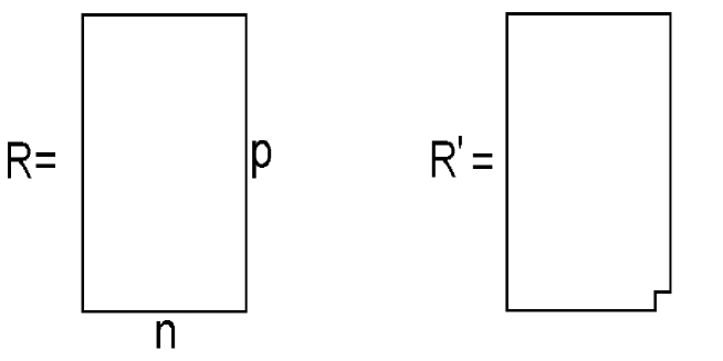
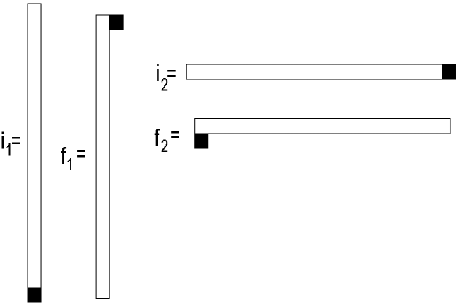
We can easily generalize the above result in two ways. First, to consider a boundstate of sphere giant gravitons, the relevant amplitude is given by

$${\cal A}_{R,R^{\prime}}={\langle\mbox{Tr\,}(Y^{\dagger J})\chi_{R^{\prime}}^{\dagger}\chi^{(1)}_{R,R^{\prime}}\rangle\over\sqrt{\langle\mbox{Tr\,}(Y^{\dagger J})\chi_{R^{\prime}}^{\dagger}\mbox{Tr\,}(Y^{J})\chi_{R^{\prime}}\rangle\langle(\chi^{(1)}_{R,R^{\prime}})^{\dagger}\chi^{(1)}_{R,R^{\prime}}\rangle}}.$$

where $R$ and $R^{\prime}$ are defined in figure 1. The computation proceeds exactly as for the single sphere giant; we will not show all of the details. The amplitude for gravitational radiation from a boundstate of $n$ sphere giants, each of angular momentum $p$ is

$${\cal A}_{R,R^{\prime}}={1\over\sqrt{n}}\sqrt{J(N-p)\over pN}.$$
Refer to caption
Figure 1: The representations used to compute the amplitude for gravitational radiation from a bound state of $n$ sphere giants. $R$ has $p$ rows and $n$ columns where $p$ is $O(N)$ and $n$ is $O(1)$. $R^{\prime}$ is obtained by removing a single box.

For a possible interpretation of this amplitude, note that there is good evidence (see for example [24]) that the giant gravitons behave as bosons. In this case, perhaps we should extract a factor of $\sqrt{n}$ from the amplitude; this factor is the usual enhancement expected as a consequence of the fact that we deal with $n$ bosons. Concretely, the interaction (the string plays no role in this argument and hence is supressed)

$$H_{int}=ga^{\dagger}_{p-1}a_{p}$$

that allows a state with $n$ identical giants of momentum $p$ to decay into a state with $n-1$ giants of momentum $p$ and one giant of momentum $p-1$, gives a matrix element proportional to $\sqrt{n}g$

$$\langle 0|{(a_{p})^{n-1}a_{p-1}\over\sqrt{(n-1)!}}H_{int}{(a_{p}^{\dagger})^{n}\over\sqrt{n!}}|0\rangle=\sqrt{n}g,$$

and not $g$ as one might naively have expected. This enhancement can be understood as a consequence of the fact that the second quantized boson creation operators automatically produces a correctly symmetrized state. Our excited giant operator is symmetric under swapping boxes in the same row and hence it too builds a correctly symmetrized state. The remaining piece of the amplitude is $O\left({1\over n}\right)$. It is naturally interpreted as a non-planar correction in the expected emergent $U(n)$ gauge theory, which should arise as the low energy world volume description of $n$ co-incident D-branes. Of course, the $U(n)$ theory does not implement this symmetrization (it is a “first quantized description” with fixed $n$) which is why the $\sqrt{n}$ factor must be included before comparing.

The amplitudes we have considered here, correspond to the situation where the endpoints of the open string join and the whole open string is emitted as a single closed string. A second generalization of the above amplitude that we can consider, is to allow a piece of the open string to pinch off, leaving a smaller open string attached to the giant. The relevant amplitude is

$${\cal A}_{(1^{p+1}),(1^{p})}(J_{1},J_{2})={\langle\mbox{Tr\,}(Y^{\dagger J_{1}})(\chi_{(1^{p+1}),(1^{p})}^{(1)}(Z,W^{(2)}))^{\dagger}\chi^{(1)}_{(1^{p+1}),(1^{p})}(Z,W^{(1)})\rangle\over\sqrt{{\cal N}_{1}{\cal N}_{2}}},$$

where

$${\cal N}_{1}=\langle\mbox{Tr\,}(Y^{\dagger J_{1}})(\chi_{(1^{p+1}),(1^{p})}^{(1)}(Z,W^{(2)}))^{\dagger}\mbox{Tr\,}(Y^{J_{1}})\chi_{(1^{p+1}),(1^{p})}^{(1)}(Z,W^{(2)})\rangle,$$
$${\cal N}_{2}=\langle(\chi^{(1)}_{(1^{p+1}),(1^{p})}(Z,W^{(1)}))^{\dagger}\chi^{(1)}_{(1^{p+1}),(1^{p})}(Z,W^{(1)})\rangle,$$

and the open strings $W^{(1)}$ and $W^{(2)}$ are

$$(W^{(1)})^{i}_{j}=(Y^{J_{1}+J_{2}})^{i}_{j}\qquad(W^{(2)})^{i}_{j}=(Y^{J_{2}})^{i}_{j}.$$

A straight forward computation gives

$${\cal A}_{(1^{p+1}),(1^{p})}(J_{1},J_{2})={\sqrt{J_{1}}(J_{2}+1)\over N}\left(1+O\left({J^{4}\over N^{2}}\right)\right).$$

This amplitude is maximized when $J_{2}$ is a maximum. Evidently it is easier for small bits of the string to break off. At this maximum value, $J_{1}=O(1)$, $J_{2}=O(J)$ with $J=J_{1}+J_{2}$ and the amplitude is of order $O\left({J\over N}\right)$. When $N-p$ is $O(N)$, the amplitude (9) is $O\left(\sqrt{J\over N}\right)$. Since ${J\over N}\ll 1$, the dominant decay process is the one in which the complete open string is emitted as a single closed string. When $N-p$ is $O(1)$, the amplitude (9) is $O\left({\sqrt{J}\over N}\right)$. In this case, the dominant decay process is the one in which small pieces of the open string pinch off.

3.1.2 Closed String Radiation from AdS Giants

The computations for AdS giants are a straight forward generalization of the computations of the previous subsection. For this reason, we do not provide all of the details. AdS giant gravitons (and bound states of them) are conjectured to be dual to operators that correspond to representations with $O(N)$ columns and $O(1)$ rows. The normalized interaction amplitude for the emission of a closed string by an excited AdS giant is given by (we use the notation $(p)$ for the symmetric representation with $p$ boxes)

$${\cal A}_{(p+1),(p)}={\langle\mbox{Tr\,}(Y^{\dagger J})\chi_{(p)}^{\dagger}\chi^{(1)}_{(p+1),(p)}\rangle\over\sqrt{\langle\mbox{Tr\,}(Y^{\dagger J})\chi_{(p)}^{\dagger}\mbox{Tr\,}(Y^{J})\chi_{(p)}\rangle\langle(\chi^{(1)}_{(p+1),(p)})^{\dagger}\chi^{(1)}_{(p+1),(p)}\rangle}}.$$

It is now a simple matter to compute

$${\cal A}_{(p+1),(p)}=\sqrt{J(N+p)\over pN}\left(1+O\left({J^{4}\over N^{2}}\right)\right).$$

For small $p$ we find that this agrees with the amplitude computed for the sphere giant. This is exactly as expected: for small values of $p$ we essentially have a point like graviton and the AdS and sphere giants are identical. However, as $p$ is increased the above amplitude decreases more slowly than the amplitude for the sphere giant. This is what we should expect. As $p$ increases it couples more strongly to the Ramond-Ramond field and the giant blows up, pushing further from the origin of AdS space. The open string attached to the giant will thus feel a greater force444Recall that the geodesic of a particle moving in AdS space is driven towards the origin.. This slower fall off of the AdS amplitude is again a manifestation of the D-brane instability discovered in [13].

We can again generalize this result to a boundstate of $n$ giants

$${\cal A}={1\over\sqrt{n}}\sqrt{J(N+p)\over pN}\left(1+O\left({J^{4}\over N^{2}}\right)\right).$$

Again, after factoring out the bosonic enhancement factor555The AdS giants do not behave as bosons. In particular, we have an upper limit of $N$ on the number of AdS giants that we can create. However, since $n<<N$, treating the AdS giants as bosons is an excellent approximation. of $\sqrt{n}$, we obtain an amplitude of $O\left({1\over n}\right)$ which is of the correct size to be identified with the first non-planar corrections of a non-Abelian gauge theory with gauge group $U(n)$. This is consistent with the expected emergent $U(n)$ gauge theory, which should arise as the low energy world volume description of $n$ co-incident AdS giant gravitons.

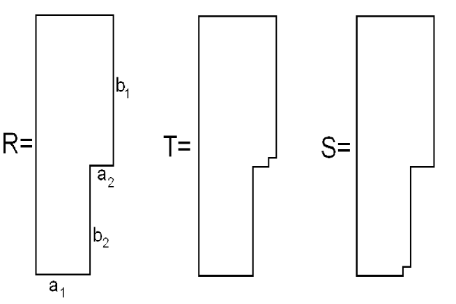
3.1.3 Probing Locality Using Closed String Radiation

Consider the representations $R$, $S$ and $T$ shown in figure 2. We are interested in the case that $b_{1}$ and $b_{2}$ are both $O(N)$ and $a_{1}$ and $a_{2}$ are both $O(1)$. The Schur polynomial $\chi_{R}(Z)$ should be dual to a bound state of $a_{1}$ giant gravitons of angular momentum $b_{1}+b_{2}$ and $a_{2}$ giant gravitons of angular momentum $b_{1}$. The radius of the giant graviton $R_{gg}$ is determined by its angular momentum $p$, in terms of the radius $R$ of the $S^{5}$ in the AdS${}_{5}\times$S5 background as

$$R_{gg}=R\sqrt{p\over N}.$$

The sphere giants wrap an S3 within the S5. Decompose the S5 as S${}^{3}\times$D2 where S3 is the sphere that the giant graviton wraps and D2 is a disk. The giant traces out a circular orbit on the disk, of radius $\sqrt{R^{2}-R_{gg}^{2}}$. Thus, the $a_{1}$ sphere giants are separated from the $a_{2}$ sphere giants by a radial distance of more than666This is the distance which separates them on the D2; the fact that their worldvolumes are S3s with different radii also contributes to the separation.

$$R\left[\sqrt{N-b_{1}\over N}-\sqrt{N-(b_{1}+b_{2})\over N}\right]=O(R).$$

Thus, for large $R$ (we work in units of the string length) we have two well separated bound states of sphere giants. The large $R$ limit corresponds to the large ’t Hooft coupling limit of the super Yang-Mills theory. Here we work in the opposite limit of zero ’t Hooft coupling. However, since we are working with operators that are nearly BPS, it is not unreasonable to hope that our results can safely be extrapolated to the strong coupling limit. For this reason, even though we work in the free field theory limit, we will still look for signals that the operator $\chi_{R}(Z)$ is dual to two well separated bound states of sphere giants. We interpret any such evidence as signals of locality in the bulk spacetime that emerges from the matrix degrees of freedom of the original Yang-Mills theory.

To start, we will compute the amplitude

$${\cal A}_{R,T}={\langle\mbox{Tr\,}(Y^{\dagger J})\chi_{T}^{\dagger}\chi^{(1)}_{R,T}\rangle\over\sqrt{\langle\mbox{Tr\,}(Y^{\dagger J})\chi_{T}^{\dagger}\mbox{Tr\,}(Y^{J})\chi_{T}\rangle\langle(\chi^{(1)}_{R,T})^{\dagger}\chi^{(1)}_{R,T}\rangle}}.$$

The natural interpretation of $\chi^{(1)}_{R,T}$ is as a bound state of $a_{1}$ sphere giants of angular momentum $b_{1}+b_{2}$ and an excited boundstate of $a_{2}$ sphere giants of angular momentum $b_{1}$. The above amplitude is easily evaluated to give

$${\cal A}_{R,T}={1\over\sqrt{a_{2}}}\sqrt{J(N-b_{1})\over Nb_{1}}\left(1+O\left({J^{4}\over N^{2}}\right)\right).$$

This is exactly what would have been obtained if the $a_{1}$ sphere giant bound state was not present. Thus, the $a_{1}$ sphere giants of momentum $b_{1}+b_{2}$ do not interact with the $a_{2}$ sphere giants of momentum $b_{1}$, which is exactly the behavior we expect from two well separated bound states.

Refer to caption
Figure 2: The representations used to test locality of sphere giants.

We can also consider the amplitude

$${\cal A}_{R,S}={\langle\mbox{Tr\,}(Y^{\dagger J})\chi_{S}^{\dagger}\chi^{(1)}_{R,S}\rangle\over\sqrt{\langle\mbox{Tr\,}(Y^{\dagger J})\chi_{S}^{\dagger}\mbox{Tr\,}(Y^{J})\chi_{S}\rangle\langle(\chi^{(1)}_{R,S})^{\dagger}\chi^{(1)}_{R,S}\rangle}}.$$

In this case, it is the bound state of $a_{1}$ sphere giants of angular momentum $b_{1}+b_{2}$ that is excited. Evaluating the above amplitude we obtain

$${\cal A}_{R,S}={1\over\sqrt{a_{1}}}\sqrt{J(N-b_{1}-b_{2})\over(b_{1}+b_{2})N}\left(1+O\left({J^{4}\over N^{2}}\right)\right).$$

Again, this is what would have been obtained if the $a_{2}$ sphere giant bound state was not present, which is again the behavior we expect from two well separated bound states.

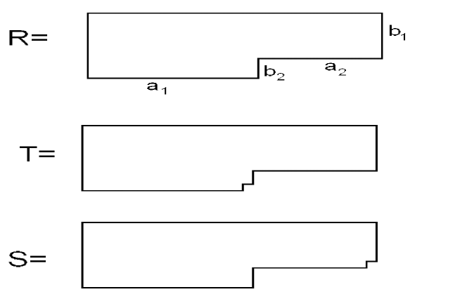
Using the sphere giants, we have been able to probe the question of locality in the S5 of the AdS${}_{5}\times$S5 background. We will now explore locality in the AdS5 part of the background using the AdS giants. As in the case of the sphere giants, the radius of the giant graviton $R_{gg}$ is determined by its angular momentum $p$, in terms of the radius $R$ of the AdS5 in the AdS${}_{5}\times$S5 background as

$$R_{gg}=R\sqrt{p\over N}.$$

Thus, the $b_{1}$ AdS giants are separated from the $b_{2}$ AdS giants by a radial distance

$$R\sqrt{a_{1}+a_{2}\over N}-R\sqrt{a_{1}\over N}=O(R).$$

The representations we will use are shown in figure 3. We assume that $a_{1}$ and $a_{2}$ are $O(N)$ and $b_{1}$ and $b_{2}$ are $O(1)$.

Refer to caption
Figure 3: The representations used to test locality of AdS giants.

Evaluating the relevant amplitudes, we obtain

$${\cal A}_{R,T}={1\over\sqrt{b_{2}}}\sqrt{J(N+a_{1})\over Na_{1}}\left(1+O\left({J^{4}\over N^{2}}\right)\right),$$
$${\cal A}_{R,S}={1\over\sqrt{b_{1}}}\sqrt{J(N+a_{1}+a_{2})\over(a_{1}+a_{2})N}\left(1+O\left({J^{4}\over N^{2}}\right)\right).$$

These amplitudes are manifestly consistent with locality in the AdS space.

3.1.4 Closed versus Open Strings

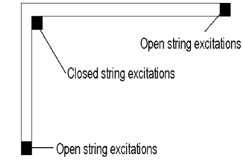
There are two types of string excitations that can be created: we can attach an open string to the membrane bound state, or we can excite a closed string. In the dual fermion language, the AdS space corresponds to a droplet. Single KK graviton excitations of this droplet corresponds to ripples on the edge of the drop. Sphere giants correspond to holes deep in the droplet, while AdS giants correspond to fermions excited well above the Fermi level. Using this dual fermion interpretation, in the Young diagram language, Berentsein has given a beautiful translation[19] of the shape of the Young diagram into membrane plus string excitations. This interpretation is summarized in figure 4.

Refer to caption
Figure 4: Translation of a Young diagram into membrane plus string excitations. The string excitations correspond to the darkened boxes.

In this section we will explore and provide further evidence for this interpretation.

Refer to caption
Figure 5: The representations used to test the interpretation of the $F_{0}$ and $F_{1}$ contributions to the two point functions. The darkened boxes represent the position of the string. There are $p$ white boxes in each diagram shown.

Consider the amplitude to make a transition from the operator corresponding to the initial state $i_{1}$ to the operator described by the final state $f_{1}$ (see figure 5)

$${\cal A}=\sqrt{J(N-p)\over Np}\left(1+O\left({J^{4}\over N^{2}}\right)\right).$$

This amplitude only recieves a contribution from the $F_{1}$ term. This is identical to the amplitude for the initial excited sphere giant state to decay into an unexcited sphere giant plus a closed string. Thus, the final state is behaving as if it is a closed string plus sphere membrane state. This is in perfect agreement with Berenstein’s picture. We can also consider the amplitude to make a transition from the operator corresponding to the initial state $i_{2}$ to the operator described by the final state $f_{2}$

$${\cal A}=\sqrt{J(N+p)\over Np}\left(1+O\left({J^{4}\over N^{2}}\right)\right).$$

Again, this amplitude only recieves a contribution from the $F_{1}$ term. This is identical to the amplitude for the initial excited AdS giant state to decay into an unexcited AdS giant plus a closed string. Thus, the final state is behaving as if it is a closed string plus AdS membrane state. Again this is in perfect agreement with Berenstein’s picture.

3.1.5 Spacetime Foam

In the subsection 3.1.3 we have managed to find some circumstantial evidence for locality in the bulk spacetime that emerges from the matrix degrees of freedom of the original Yang-Mills theory. It is interesting (and comforting) to see this locality emerge in a situation where it is expected. It is equally interesting to ask how locality breaks down, a question that should provide some insight into what happens at the Planck scale in a theory of quantum gravity. In the regime in which locality does break down, we expect that quantum gravity corrections become important. As a first step towards probing these issues, in this section we will study the correlation functions of operators which are described in the dual quantum gravity by a “spacetime foam”. The low energy effective description of a foam[24] with given global charges is in terms of the superstar geometry[32], which is singular. For very interesting and insightful related work see[33].

We have already mentioned that as the number of boxes in the Young diagram changes, the interpretation of the operator in the dual gravitational theory changes: for $\sim 1$ boxes the operator is dual to a supergravity state, for $\sim\sqrt{N}$ boxes the operator is dual to a string state and for $\sim N$ boxes the operator is dual to a giant graviton. In this section we consider operators with $\sim N^{2}$ boxes. In this case, the operator is dual to a new geometry.

The two point function of an excited giant with a single string attached receives two contributions, depending on how the associated open string words contract. We have denoted these two open string contributions as $F_{0}$ and $F_{1}$. In the preceding subsections, the term proportional to $F_{0}$ has been the dominant contribution to the normalization factor of the amplitudes we computed. Given the way the indices of the string contract, it is natural to interpret this term as an open string overlap. $F_{0}$ enters when we compute the normalization of an operator. By the same logic, the term proportional to $F_{1}$ is naturally interpreted as a closed string interaction. $F_{1}$ naturally enters when we compute the transition amplitude between two states: the open string “peels” off the boundstate to form a closed string and then “reattaches” as an open string in a new position. In this section, we will ask if there are operators $\chi_{R,R^{\prime}}^{(1)}$, such that the contributions from the $F_{1}$ and $F_{0}$ terms to the two point function are of the same order of magnitude. Presumably, the geometries dual to these operators have Planck scale features implying high curvatures, so that the corrections to the leading result are important.

Consider attaching a single string to our boundstate of giants. Using the rules from section 2.5, we know that the two point function takes the form

$$\langle(\chi_{R,R^{\prime}}^{(1)})^{\dagger}\chi_{R,R^{\prime}}^{(1)}\rangle=nF_{0}f_{R}{d_{R^{\prime}}\over d_{R}}+F_{1}c_{R,R^{\prime}}^{2}f_{R^{\prime}},$$

where $n$ is the number of boxes in the Young diagram, $c_{R,R^{\prime}}$ is the weight of the box that must be removed from $R$ to obtain $R^{\prime}$ and $d_{R},d_{R^{\prime}}$ are the dimensions of the $R,R^{\prime}$ representations of the symmetric groups $S_{n},S_{n-1}$. Now, we know that $f_{R}=c_{R,R^{\prime}}f_{R^{\prime}}.$ Thus, we are looking for representations $R$ such that

$$nF_{0}{d_{R^{\prime}}\over d_{R}}\sim F_{1}c_{R,R^{\prime}}.$$

In the limit that we consider ($J^{2}N\ll 1$) $F_{0}$ dominates $F_{1}$. Thus, we need to find representations $R$ for which

$${d_{R^{\prime}}\over d_{R}}\ll 1.$$

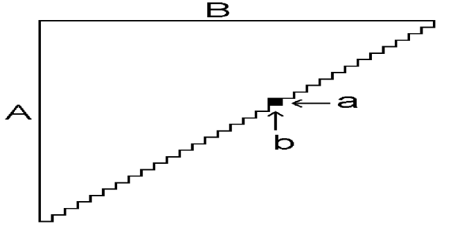
This will be the case if representation $R$ can subduce many different representations $R^{\prime}$. The set of all possible representations that can be subduced from a given Young diagram $R$ is given by the set of all Young diagrams that can be obtained by removing a single box from $R$. Since we can remove any box that is a corner, this naturally suggests that we should consider representations $R$ which correspond to Young diagrams that have a very large number of corners. An example of such a Young diagram is given in figure 6.

Refer to caption
Figure 6: The representation $R$ shown has the maximum number of “corners” possible. As a result, it subduces a large number of representations when a single box is removed. $R^{\prime}$ is obtained by removing the filled box. The filled box is in row $a$ and column $b$. We consider the case that $A$ and $B$ are both $O(N)$.

The quantities appearing in our two point function are

$\displaystyle n{d_{R^{\prime}}\over d_{R}}$ $\displaystyle=$ $\displaystyle{(A-a+b)!!\over(A-a+b-1)!!}{(B+a-b)!!\over(B+a-b-1)!!}$ (10)
$\displaystyle=$ $\displaystyle{\left[(A-a+b)!!\right]^{2}\over(A-a+b)!}{\big{[}(B+a-b)!!\big{]}^{2}\over(B+a-b)!},$ (11)
$\displaystyle c_{R,R^{\prime}}$ $\displaystyle=$ $\displaystyle N-a+b.$

We will consider the case that $b=O(N)$, $a=O(1)$ so that $A-a+b=O(N)$ and $B+a-b=O(1)$. Using Stirling’s approximation to evaluate the above factorials we find

$$n{d_{R^{\prime}}\over d_{R}}={e^{2}\sqrt{2}\over\sqrt{\pi}}\sqrt{A-a+b}.$$

Clearly, $c_{R,R^{\prime}}$ is $O(N)$. Taking the open string word

$$(W)^{i}_{j}=(Y^{J})^{i}_{j}$$

with $J^{2}N$ fixed, we easily find

$$nF_{0}{d_{R^{\prime}}\over d_{R}}\sim\sqrt{A-a+b}N^{J-1},\qquad F_{1}c_{R,R^{\prime}}\sim(J-1)N^{J-1}.$$

Thus, the corrections to the leading term are the same size as the leading term. It is interesting to note that triangular Young diagrams were studied in [24],[33] where they were argued to be relevant for a description of the geometry of the superstar[32] and further were used to show that they are described by an effective geometry that is singular. This singular geometry was interpreted as an effective description of microstates that differ from each other by Planck scale structures. See [34] for a connection to ${\cal R}$ charged black holes in AdS${}_{5}\times$S5.

Based on the results of this section, it is clear that the number of corners in the Young diagram provides important information about the dual effective geometry. The importance of the corners in Young tableaux is clear from the LLM solution: the number of corners is the number of edges of LLM geometries with circular symmetry. If the diagram has $O(1)$ corners and $O(N)$ boxes, it should be described by a smooth effective geometry. If the diagram has $O(N)$ corners, the corresponding microstates exhibit Planck scale structure and should be described by a singular effective geometry. The number of corners translates roughly into the number of distiguishable bunches of D-branes. More corners implies more distinguishable D-branes, and hence more possible open strings excitations. Thus, brane systems described by Young diagrams with many corners have many nearby states that can be explored, implying a large entropy, signaling that one is getting nearer to a black hole state777We thank David Berenstein for suggesting this explanation to us..

3.2 Interacting Giants

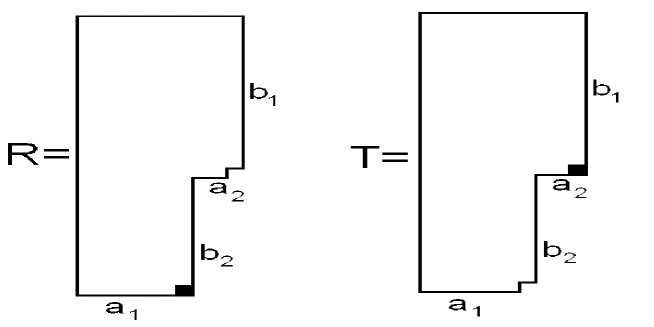
In this section we will consider the process in which an excited giant graviton makes a transition from one excited state to another excited state. The amplitude for this process is given by

$${\cal A}={{\langle(\chi_{R,R^{\prime}}^{(1)}})^{\dagger}\chi^{(1)}_{T,T^{\prime}}\rangle\over\sqrt{\langle(\chi_{R,R^{\prime}}^{(1)})^{\dagger}\chi_{R,R^{\prime}}^{(1)}\rangle\langle(\chi^{(1)}_{T,T^{\prime}})^{\dagger}\chi^{(1)}_{T,T^{\prime}}\rangle}}.$$

The representations $R,R^{\prime}$ and $T,T^{\prime}$ are defined in figure 7. When we consider the case that $b_{1}$ and $b_{2}$ are $O(N)$ and $a_{1}$ and $a_{2}$ are $O(1)$, this process looks like the open string attached to the bound state of $a_{1}$ sphere giants (of angular momentum $b_{1}+b_{2}$) is emitted and then absorbed by the bound state of $a_{2}$ sphere giants (of angular momentum $b_{1}$). The leading contribution to the amplitude for this process is given by

$${\cal A}={1\over\sqrt{a_{1}}}\sqrt{J(N-b_{1}-b_{2})\over N(b_{1}+b_{2})}\times{1\over\sqrt{a_{2}}}\sqrt{J(N-b_{1})\over Nb_{1}}\left(1+O\left({J^{4}\over N^{2}}\right)\right).$$

Notice that this amplitude is a product of the amplitude for the first bound state to emit a string times the amplitude for the second bound state to absorb the string. This is what one would guess for the amplitude if one assumes a local cubic interaction, and if in addition the amplitude for a closed string to propagate from the first bound state to the second bound state is 1. This second assumption is very natural, since in the free field theory limit that we consider, the background is small in units of the string length.

We could also consider the case that $a_{1}$ and $a_{2}$ are $O(N)$ and $b_{1}$ and $b_{2}$ are $O(1)$. In this case, the process we are studying looks like an open string attached to the bound state of $b_{1}$ AdS giants (of angular momentum $a_{1}+a_{2}$) is emitted and then absorbed by the bound state of $b_{2}$ AdS giants (of angular momentum $a_{1}$). The leading contribution to the amplitude for this process is given by

$${\cal A}={1\over\sqrt{b_{1}}}\sqrt{J(N+a_{1}+a_{2})\over N(a_{1}+a_{2})}\times{1\over\sqrt{b_{2}}}\sqrt{J(N+a_{1})\over Na_{1}}\left(1+O\left({J^{4}\over N^{2}}\right)\right).$$

Again, this amplitude is a product of the amplitude for the first bound state to emit a string times the amplitude for the second bound state to absorb the string. Both transition amplitudes received a contribution only from the $F_{1}$ term.

Refer to caption
Figure 7: The representations $R$ and $T$ used to compute the amplitude for a transition between two excited giant graviton states. $R^{\prime}$ and $T^{\prime}$ are obtained by removing the filled box from $R$ and $T$ respectively.

3.3 Splitting and Joining

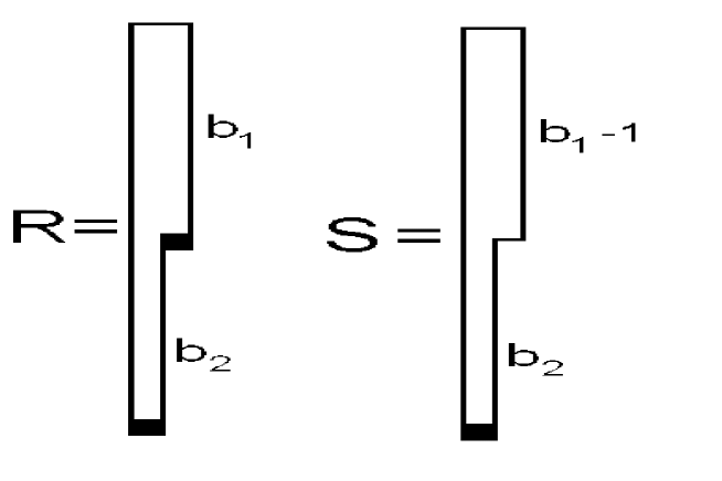
The open strings that live on the world volume of the giant gravitons interact by splitting and joining. In this subsection we consider the simplest possible process of two strings in their ground states joining into one. The operators with one and two string excitations are defined using the representations given in figure 8. The normalized amplitude for the string joining process is given by

$${\cal A}={\langle(\chi^{(1)}_{S,S^{\prime}})^{\dagger}\chi^{(2)}_{R,R^{\prime\prime}}\rangle\over\sqrt{\langle(\chi^{(1)}_{S,S^{\prime}})^{\dagger}\chi^{(1)}_{S,S^{\prime}}\rangle\langle(\chi^{(2)}_{R,R^{\prime\prime}})^{\dagger}\chi^{(2)}_{R,R^{\prime\prime}}\rangle}}.$$

The correlator in the numerator will be related to the open string field theory vertex for the open string field theory describing the strings attached to a giant graviton. A discussion of this point for the case of BMN operators can be found in[35]. The open strings attached to $\chi^{(2)}_{R,R^{\prime\prime}}$ are given by

$$W^{(1)}=Y^{J_{1}},\qquad W^{(2)}=Y^{J_{2}}.$$

The open string attached to $\chi^{(1)}_{S,S^{\prime}}$ is given by

$$W=Y^{J_{1}+J_{2}}.$$

The computation of the denominator is straight forward using the rules given in section 2.5. The computation of the correlator in the numerator factorizes into a contribution from the open string words and a contribution from contracting the $Z$s. The open string correlator is treated in appendix G. We keep only the leading contribution, that is, the terms labeled $e$ and $f$ in appendix G. The contribution coming from contracting the $Z$s is treated in appendix H. Using these results, we find that the leading contribution to the amplitude is given by

Refer to caption
Figure 8: The representations used in the computation of the string joining amplitude. The representation $R^{\prime}$ is obtained by dropping the filled box in the second column of $R$. The representation $R^{\prime\prime}$ is obtained by dropping both filled boxes from $R$. The representation $S^{\prime}$ is obtained by dropping the filled box from $S$. We consider the situation that $b_{1}$ is $O(N)$ and $b_{2}$ is $O(1)$ and $b_{2}\gg 1$.
$${\cal A}=2\sqrt{N-b_{1}\over Nb_{1}}{1\over b_{2}+1}\left(1+O\left({J^{4}\over N^{2}}\right)\right).$$

We take $b_{1}$ to be $O(N)$ and $b_{2}$ to be $O(1)$. Thus, the two strings which join are on branes that are nearby in spacetime. For this reason, we expect that we are probing the dynamics of the brane world volume theory. Notice that this amplitude is independent of the angular momentum of the open strings which join. To interpret this amplitude, note that arguing exactly as in section 3.1.3, the two open strings that are interacting are separated by a distance of ($R$ is the radius of the S5)

$$r=R\left[\sqrt{N-b_{1}\over N}-\sqrt{N-b_{1}-b_{2}\over N}\right]\approx{Rb_{2}\over 2\sqrt{N(N-b_{1})}}.$$

The distance $r$ between the two interacting strings is determined by $b_{2}$. $b_{2}$ itself is obtained by counting how many boxes on the Young diagram we pass through when moving on the right most edge of the Young diagram, between the two strings that are interacting888We find that this is generally the case for string splitting/joining amplitudes: for general choices of representations $R$ and $S$, the joining/splitting amplitude falls off as the inverse of the number of boxes on the Young diagram we pass through when moving on the right most edge of the Young diagram, between the two strings that are interacting.. This is another indication that the geometry is coded into the Young diagram labeling the operator. There is a connection between the coordinate that we have identified here and the coordinates employed by LLM[23]. Recall that the boundary conditions for the LLM solutions are specified by droplets on the $y=0$ plane. The radial coordinate on the $y=0$ plane is the distance $r$ we have just introduced. The fact that the string sigma model dynamics simplifies when expressed using these LLM coordinates was emphasized in [36]. In terms of this distance, we can write the amplitude for string joining as (we approximate $b_{2}+1\approx b_{2}$)

$${\cal A}={R\over N\sqrt{b_{1}}}{1\over r}.$$

To reproduce this amplitude in Born approximation we would need a ${1\over r}$ (quark-antiquark) potential in the brane world volume theory. Assume that the dominant contribution to this potential will arise from the exchange of massless particles. To reproduce the potential implied by our amplitude we see that the emergent Yang-Mills theory is a 3+1 dimensional theory.

Although the fact that we have obtained a ${1\over r}$ potential is encouraging, our argument is not as clean as we would like. Indeed, if it is possible, we would have liked to separate the two open strings in the directions belonging to the emergent world volume, and place them at an equal radial distance. The separation appearing in our calculation is, if our naive interpretation is correct, seems to be in the radial direction.

4 Discussion

In this paper we have initiated a systematic study of the operators dual to giant gravitons with open strings attached to them. We have introduced a graphical notation, which employs Young diagrams, for these operators. The computation of two point correlation functions has been reduced to the application of three simple rules, which were summarized in section 2.5. The rules themselves are written as graphical operations performed on the Young diagram labels of the operators and the final result for the correlation function is read directly off these labels. As a test of our results, we have written code to numerically compute the values of a number of correlators. Our graphical rules are in complete agreement with this “experimental data”. Using this technology, we have studied gravitational radiation by giant gravitons and bound states of giant gravitons, transitions between excited giant graviton states and joining of open strings attached to the giant. The results of our study suggest a number of interesting conclusions:

  • The Young diagram labeling of the operators dual to giant gravitons originally introduced to study the $c=1$ matrix model by Jevicki[37] and in the ${\cal N}=4$ super Yang-Mills context by Corley, Jevicki and Ramgoolam, continues to provide a useful labeling in the more general situation where the operators are dual to excited giant gravitons.

  • We have studied operators labeled by Young diagrams with $m=O(1)$ columns, each having $p=O(N)$ rows. These are expected to be dual to a bound state of $m$ coincident sphere giants. The expected world volume theory of these $m$ sphere giants is a 3+1 dimensional Yang-Mills theory with gauge group $U(m)$. This emergent theory should be local on a space built out of the matrix degrees of freedom of the original Yang-Mills theory. Thus this is a concrete toy model that can be used to study how extra dimensions arise from matrix models. We have found some evidence for this conjectured $U(m)$ emergent gauge theory. After extracting the usual bosonic enhancement factor of $\sqrt{m}$ from the amplitude for gravitational radiation from a bound state of $m$ giant gravitons, we find an amplitude of $O\left({1\over m}\right)$, which is the correct size to be interpreted as a non-planar correction in a Yang-Mills theory with gauge group $U(m)$. Further, by studying string joining and splitting we have found evidence for a quark-antiquark potential that drops as ${1\over r}$, with $r$ the distance between the quark and the antiquark. This may be a signal that the emergent gauge theory has three spatial dimensions. The distance $r$ is defined by counting how many boxes on the Young diagram we pass through when moving on the right most edge of the Young diagram, between the two strings that are interacting. This is just one of many examples where we have an indication that the geometry is coded into the Young diagram labeling the operator.

  • Operators labeled by Young diagrams with $m=O(1)$ rows, each having $p=O(N)$ columns are dual to a bound state of AdS giants. We have again found evidence that the world volume theory of these $m$ AdS giants is described by a 3+1 dimensional Yang-Mills theory with gauge group $U(m)$.

  • We have found signals of locality in the bulk spacetime. To probe this issue, the basic process we have considered is the emission of a closed string from a bound state of excited giant gravitons that are separated from a second (unexcited) bound state. We have some evidence that widely separated bound states of giant gravitons do not interact with each other.

  • We have studied transitions between excited giant graviton states. The operators we use for the study of transitions are naturally interpreted as dual to states of widely separated bound states of giant gravitons. The transitions we study correspond to the process where an open string attached to one of the bound states is emitted and reabsorbed by the second bound state. The amplitude can be written neatly as the product of the amplitude for the first bound state to emit a closed string with the amplitude for the second bound state to absorb a closed string. This suggests that a description of the dynamics employing the giant graviton and string degrees of freedom will be a local theory with a cubic interaction vertex. It is also interesting to ask if, using amplitude calculations of the type we have explored, such a dynamical description can be constructed. For relevant related work directed at (unexcited) giant gravitons see for example[38] and for work directed at strings see for example [39].

  • Our two point correlators for giants with a single string attached receive two contributions, distinguished by how the open string words are contracted. We have seen that these two contributions are naturally interpreted as a leading (open string overlap) term and a (closed string interaction) correction term. The leading term determines the normalizations of our amplitudes. The correction determines transition amplitudes. We have been able to describe the circumstances in which the correction is the same size as the leading term. In these situations we expect that quantum gravity corrections become important and classical notions, such as spacetime and locality, may not be applicable. Our results show that the number of corners in the Young diagram provides important information about the dual effective geometry. If the diagram has $O(1)$ corners and $O(N)$ boxes, it should be described by a smooth effective geometry. If the diagram has $O(N)$ corners, the corresponding microstates exhibit Planck scale structure and should be described by a singular effective geometry. This is natural in view of the LLM solutions: a Young diagram with many corners corresponds to having many concentric, thin black rings on the $y=0$ plane. Since thin rings will effectively be averaged in a low energy description, this leads to a gray disk on the $y=0$ plane which does lead to a singular geometry. These conclusions are consistent with the notion of the quantum foam described in [24].

  • We find a nice confirmation of the physical picture developed in [19]. This allows us to translate a given restricted Schur polynomial into giant graviton bound state plus a specific set of string excitations. String words added at the end of a long row or a long column correspond to open string excitations of the giant graviton bound state. String words added in row $i$ and column $j$ with both $i$ and $j$ $O(1)$ describe closed strings.

One deficiency of our work, is that our results apply only in the zero coupling limit of the theory. In a second article [17], we will show that the action of the $F$-terms can also be summarized by a simple graphical rule. This allows us to account for the first perturbative correction to the free field theory answer.

Acknowledgements: We would like to thank Michael Abbott, David Bekker, Sera Cremonini, Aristomenis Donos, Antal Jevicki, Jeff Murugan, Sanjaye Ramgoolam, Joao Rodrigues, Michael Stephanou, Alex Welte and especially David Berenstein, for pleasant discussions and/or helpful correspondence. This work is supported by NRF grant number Gun 2047219.

Appendix A Reduction Formula for Schur Polynomials

In this appendix we prove the reduction formula discovered in [21]. Our strategy is to exploit known recursion relations obeyed by Schur polynomials corresponding to the completely symmetric and antisymmetric representations to prove the reduction formula for these representations. We then recall the rewriting of an arbitrary Schur polynomial in terms of the determinant of a matrix whose elements are Schur polynomials of only the symmetric or antisymmetric representations. Using this relation and the already established result, we extend the proof of the reduction rule to an arbitrary Schur polynomial.

A.1 Statement of the Reduction Rule

Consider a Schur polynomial $\chi_{(\lambda_{1},\lambda_{2},\cdots,\lambda_{r})}$ with $r$ rows and $\lambda_{i}$ boxes in the $i^{th}$ row. The reduction rule we wish to prove says that the reduction of the Schur polynomial is given by summing all Schur polynomials that can be obtained by removing a single box to leave a valid Young diagram, and weighting each such term by the weight of the removed box999Recall that the box in the $i^{th}$ row (counting the top row as 1 and increasing by one for each row below it) and $j^{th}$ column (counting the leftmost column as 1 and increasing by one for each column to the right) has weight $N-i+j$.

$\displaystyle D\chi_{(\lambda_{1},\lambda_{2},\cdots,\lambda_{r})}$ $\displaystyle=$ $\displaystyle(N+\lambda_{1}-1)\chi_{(\lambda_{1}-1,\lambda_{2},\cdots,\lambda_{r})}+(N+\lambda_{2}-2)\chi_{(\lambda_{1},\lambda_{2}-1,\cdots,\lambda_{r})}+\cdots$
$\displaystyle\quad+(N+\lambda_{r}-r)\chi_{(\lambda_{1},\lambda_{2},\cdots,\lambda_{r}-1)}.$

A.2 Symmetric Representations

The Schur polynomials corresponding to the completely symmetric representations $\chi_{(k)}(Z)$ obey Brioschi’s formulae[40]

$$\chi_{(k)}(Z)={1\over k}\sum_{p=1}^{k}\mbox{Tr\,}(Z^{p})\chi_{(k-p)}(Z).$$

In the above relation, $\chi_{(0)}(Z)=1$ and $\chi_{(1)}(Z)=\mbox{Tr\,}Z$. Clearly,

$$D\chi_{(0)}(Z)=0,\qquad D\chi_{(1)}(Z)=N=N\chi_{(0)}(Z).$$

Make the inductive hypothesis

$$D\chi_{(l)}=(N+l-1)\chi_{(l-1)}(Z),\qquad k>l\geq 1,$$ (14)

which we have proved for $l=1$. Reducing Brioschi’s formulae we have

$$D\chi_{(k)}(Z)={1\over k}\sum_{p=1}^{k}\left(D\mbox{Tr\,}(Z^{p})\chi_{(k-p)}(Z)+\mbox{Tr\,}(Z^{p})D\chi_{(k-p)}(Z)\right).$$

Use the inductive hypothesis and $D\mbox{Tr\,}(Z^{p})=p\mbox{Tr\,}(Z^{p-1})$ to obtain ($\chi_{(-1)}(Z)\equiv 0$)

$\displaystyle D\chi_{(k)}(Z)$ $\displaystyle=$ $\displaystyle{1\over k}\sum_{p=1}^{k}\left(p\mbox{Tr\,}(Z^{p-1})\chi_{(k-p)}(Z)+\mbox{Tr\,}(Z^{p})(N+k-p-1)\chi_{(k-p-1)}(Z)\right)$ (15)
$\displaystyle=$ $\displaystyle{N+k\over k}\sum_{p=1}^{k-1}\mbox{Tr\,}(Z^{p})\chi_{(k-p-1)}(Z)+{N\over k}\chi_{(k-1)}(Z)$
$\displaystyle=$ $\displaystyle{N+k\over k}(k-1)\chi_{(k-1)}+{N\over k}\chi_{(k-1)}=(N+k-1)\chi_{(k-1)}(Z).$

To get the last line above, we again used Brioschi’s formulae. This furnishes a proof by induction of (14).

A.3 Antisymmetric Representations

The Schur polynomials corresponding to the completely antisymmetric representations $\chi_{(1^{k})}(Z)$ obey Newton’s formulae[40]

$$\chi_{(1^{k})}(Z)={1\over k}\sum_{p=1}^{k}(-1)^{p-1}\mbox{Tr\,}(Z^{p})\chi_{(1^{k-p})}(Z).$$

In the above relation, $\chi_{(1^{0})}(Z)=1$ and $\chi_{(1^{1})}(Z)=\mbox{Tr\,}Z$. Clearly,

$$D\chi_{(1^{0})}(Z)=0,\qquad D\chi_{(1^{1})}(Z)=N=N\chi_{(1^{0})}(Z).$$

Make the inductive hypothesis

$$D\chi_{(1^{l})}=(N-l+1)\chi_{(1^{l-1})}(Z),\qquad k>l\geq 1,$$ (17)

which we have proved for $l=1$. Reducing Newton’s formulae we have

$$D\chi_{(1^{k})}(Z)={1\over k}\sum_{p=1}^{k}(-1)^{p-1}\left(D\mbox{Tr\,}(Z^{p})\chi_{(1^{k-p})}(Z)+\mbox{Tr\,}(Z^{p})D\chi_{(1^{k-p})}(Z)\right).$$

Use the inductive hypothesis and $D\mbox{Tr\,}(Z^{p})=p\mbox{Tr\,}(Z^{p-1})$ to obtain ($\chi_{(1^{-1})}(Z)\equiv 0$)

$\displaystyle D\chi_{(1^{k})}(Z)$ $\displaystyle=$ $\displaystyle{1\over k}\sum_{p=1}^{k}(-1)^{p-1}\left(p\mbox{Tr\,}(Z^{p-1})\chi_{(1^{k-p})}(Z)\right.$ (19)
$\displaystyle\qquad\left.+\mbox{Tr\,}(Z^{p})(N-k+p+1)\chi_{(1^{k-p-1})}(Z)\right)$
$\displaystyle=$ $\displaystyle{N-k\over k}\sum_{p=1}^{k-1}(-1)^{p-1}\mbox{Tr\,}(Z^{p})\chi_{(1^{k-p-1})}(Z)+{N\over k}\chi_{(1^{k-1})}(Z)$
$\displaystyle=$ $\displaystyle{N-k\over k}(k-1)\chi_{(1^{k-1})}+{N\over k}\chi_{(1^{k-1})}=(N-k+1)\chi_{(1^{k-1})}(Z).$

To get the last line above, we again used Newton’s formulae. This furnishes a proof by induction of (17).

A.4 General Representations

An arbitrary Schur polynomial can be expressed as[40]

$$\chi_{(\lambda_{1},\lambda_{2},\cdots,\lambda_{r})}=\det(\chi_{(\lambda_{i}-i+j)}).$$ (21)

As an example of this formula, it is simple to verify that

χ                     =det[χ     χ     χ     χ     ].subscript𝜒                     delimited-[]matrixsubscript𝜒     subscript𝜒     subscript𝜒     subscript𝜒     \chi_{\hbox{}{\vbox{\offinterlineskip\vbox{\hrule height=0.3pt\hbox{\vrule height=4.30496pt,width=0.3pt,depth=1.9133pt\hbox to4.78333pt{\hfil}\vrule height=4.30496pt,width=0.3pt,depth=1.9133pt\hbox to4.78333pt{\hfil}\vrule height=4.30496pt,width=0.3pt,depth=1.9133pt\hbox to4.78333pt{\hfil}\vrule height=4.30496pt,width=0.3pt,depth=1.9133pt} \hrule height=0.3pt}\vspace{-\y@linethick} \vbox{\hrule height=0.3pt\hbox{\vrule height=4.30496pt,width=0.3pt,depth=1.9133pt\hbox to4.78333pt{\hfil}\vrule height=4.30496pt,width=0.3pt,depth=1.9133pt\hbox to4.78333pt{\hfil}\vrule height=4.30496pt,width=0.3pt,depth=1.9133pt} \hrule height=0.3pt}\vspace{-\y@linethick} }}}=\det\left[\matrix{\chi_{\hbox{}{\vbox{\offinterlineskip\vbox{\hrule height=0.3pt\hbox{\vrule height=4.30496pt,width=0.3pt,depth=1.9133pt\hbox to4.78333pt{\hfil}\vrule height=4.30496pt,width=0.3pt,depth=1.9133pt\hbox to4.78333pt{\hfil}\vrule height=4.30496pt,width=0.3pt,depth=1.9133pt\hbox to4.78333pt{\hfil}\vrule height=4.30496pt,width=0.3pt,depth=1.9133pt} \hrule height=0.3pt}\vspace{-\y@linethick} }}}&\chi_{\hbox{}{\vbox{\offinterlineskip\vbox{\hrule height=0.3pt\hbox{\vrule height=4.30496pt,width=0.3pt,depth=1.9133pt\hbox to4.78333pt{\hfil}\vrule height=4.30496pt,width=0.3pt,depth=1.9133pt\hbox to4.78333pt{\hfil}\vrule height=4.30496pt,width=0.3pt,depth=1.9133pt\hbox to4.78333pt{\hfil}\vrule height=4.30496pt,width=0.3pt,depth=1.9133pt\hbox to4.78333pt{\hfil}\vrule height=4.30496pt,width=0.3pt,depth=1.9133pt} \hrule height=0.3pt}\vspace{-\y@linethick} }}}\cr\chi_{\hbox{}{\vbox{\offinterlineskip\vbox{\hrule height=0.3pt\hbox{\vrule height=4.30496pt,width=0.3pt,depth=1.9133pt\hbox to4.78333pt{\hfil}\vrule height=4.30496pt,width=0.3pt,depth=1.9133pt} \hrule height=0.3pt}\vspace{-\y@linethick} }}}&\chi_{\hbox{}{\vbox{\offinterlineskip\vbox{\hrule height=0.3pt\hbox{\vrule height=4.30496pt,width=0.3pt,depth=1.9133pt\hbox to4.78333pt{\hfil}\vrule height=4.30496pt,width=0.3pt,depth=1.9133pt\hbox to4.78333pt{\hfil}\vrule height=4.30496pt,width=0.3pt,depth=1.9133pt} \hrule height=0.3pt}\vspace{-\y@linethick} }}}}\right].

Using the already established reduction formula for the Schur polynomials of the symmetric representations we obtain

$$D\chi_{(\lambda_{1},\lambda_{2},\cdots,\lambda_{r})}=\sum_{k=1}^{r}\det(\chi^{k,a}_{(\lambda_{i}-i+j)})+\sum_{k=1}^{r}\det(\chi^{k,b}_{(\lambda_{i}-i+j)}),$$

where

$\displaystyle\chi^{k,a}_{(\lambda_{i}-i+j)}$ $\displaystyle=$ $\displaystyle\chi_{(\lambda_{i}-i+j)},\qquad i\neq k$
$\displaystyle=$ $\displaystyle(N+\lambda_{i}-i)\chi_{(\lambda_{i}-i+j-1)}\qquad i=k,$
$\displaystyle\chi^{k,b}_{(\lambda_{i}-i+j)}$ $\displaystyle=$ $\displaystyle\chi_{(\lambda_{i}-i+j)},\qquad i\neq k$
$\displaystyle=$ $\displaystyle(j-1)\chi_{(\lambda_{i}-i+j-1)}\qquad i=k,$

The term $\sum_{k=1}^{r}\det(\chi^{k,b}_{(\lambda_{i}-i+j)})$ can be organized to give a sum of terms

$$\sum_{k=1}^{r}\det(\chi^{k,b}_{(\lambda_{i}-i+j)})=\sum_{i=2}^{r}\,T_{i},$$

with the following structure ($T_{i}$ is a sum of $r$ terms)

$$T_{i}=\det\left[\matrix{0&0&\cdots&0&A_{1,i-1}&A_{1,i}&\cdots&A_{1,r-1}\cr A_{2,1}&A_{2,2}&\cdots&A_{2,i-1}&A_{2,i}&A_{2,i+1}&\cdots&A_{2,r}\cr A_{3,1}&A_{3,2}&\cdots&A_{3,i-1}&A_{3,i}&A_{3,i+1}&\cdots&A_{3,r}\cr:&:&\cdots&:&:&:&\cdots&:\cr A_{r,1}&A_{r,2}&\cdots&A_{r,i-1}&A_{r,i}&A_{r,i+1}&\cdots&A_{r,r}}\right]$$
$$\,+\det\left[\matrix{A_{1,1}&A_{1,2}&\cdots&A_{1,i-1}&A_{1,i}&A_{1,i+1}&\cdots&A_{1,r}\cr 0&0&\cdots&0&A_{2,i-1}&A_{2,i}&\cdots&A_{2,r-1}\cr A_{3,1}&A_{3,2}&\cdots&A_{3,i-1}&A_{3,i}&A_{3,i+1}&\cdots&A_{3,r}\cr:&:&\cdots&:&:&:&\cdots&:\cr A_{r,1}&A_{r,2}&\cdots&A_{r,i-1}&A_{r,i}&A_{r,i+1}&\cdots&A_{r,r}}\right]+\cdots$$
$$+\,\det\left[\matrix{A_{1,1}&A_{1,2}&\cdots&A_{1,i-1}&A_{1,i}&A_{1,i+1}&\cdots&A_{1,r}\cr A_{2,1}&A_{2,2}&\cdots&A_{2,i-1}&A_{2,i}&A_{2,i+1}&\cdots&A_{2,r}\cr A_{3,1}&A_{3,2}&\cdots&A_{3,i-1}&A_{3,i}&A_{3,i+1}&\cdots&A_{3,r}\cr:&:&\cdots&:&:&:&\cdots&:\cr 0&0&\cdots&0&A_{r,i-1}&A_{r,i}&\cdots&A_{r,r-1}}\right].$$

Expanding the determinants for any given $T_{i}$ the coefficient of any given monomial vanishes. For example, consider the coefficient of the monomial $A_{11}A_{21}\prod_{m=3}^{n}A_{mm}$ coming from $T_{1}$. Only the first two terms contribute and they give

$$\epsilon^{2134\cdots n}+\epsilon^{1234\cdots n}=0.$$

Thus,

$$\sum_{k=1}^{r}\det(\chi^{k,b}_{(\lambda_{i}-i+j)})=0,$$

so that

$\displaystyle D\chi_{(\lambda_{1},\lambda_{2},\cdots,\lambda_{r})}$ $\displaystyle=$ $\displaystyle\sum_{k=1}^{r}\det(\chi^{k,a}_{(\lambda_{i}-i+j)})$ (24)
$\displaystyle=$ $\displaystyle(N+\lambda_{1}-1)\chi_{(\lambda_{1}-1,\lambda_{2},\cdots,\lambda_{r})}+(N+\lambda_{2}-2)\chi_{(\lambda_{1},\lambda_{2}-1,\cdots,\lambda_{r})}+\cdots$
$\displaystyle\quad+(N+\lambda_{r}-r)\chi_{(\lambda_{1},\lambda_{2},\cdots,\lambda_{r}-1)},$

which is the reduction rule for the general Schur polynomial. To obtain the last equality, we needed to use the result (21). In using (21), only terms which correspond to a valid Young diagram give a non-zero contribution, so that only these terms should be included in the final result above.

We can give an alternative proof of exactly the same result, by writing the arbitrary Schur polynomial in terms of the Schur polynomials corresponding to the totally antisymmetric representations. For the Schur polynomial $\chi_{(\lambda_{1},\lambda_{2},\cdots,\lambda_{r})}$, let $\mu_{i}$ denote the number of boxes in the $i^{th}$ column. The alternative proof uses the formula[40]

$$\chi_{(\lambda_{1},\lambda_{2},\cdots,\lambda_{r})}=\det(\chi_{(1^{\mu_{i}-i+j})}).$$

A.5 Examples

To illustrate the reduction rule, we end this appendix with two examples

Dχ                     =(N+2)χ                   +Nχ                   ,𝐷subscript𝜒                     𝑁2subscript𝜒                   𝑁subscript𝜒                   D\chi_{\hbox{}{\vbox{\offinterlineskip\vbox{\hrule height=0.3pt\hbox{\vrule height=4.30496pt,width=0.3pt,depth=1.9133pt\hbox to4.78333pt{\hfil}\vrule height=4.30496pt,width=0.3pt,depth=1.9133pt\hbox to4.78333pt{\hfil}\vrule height=4.30496pt,width=0.3pt,depth=1.9133pt\hbox to4.78333pt{\hfil}\vrule height=4.30496pt,width=0.3pt,depth=1.9133pt} \hrule height=0.3pt}\vspace{-\y@linethick} \vbox{\hrule height=0.3pt\hbox{\vrule height=4.30496pt,width=0.3pt,depth=1.9133pt\hbox to4.78333pt{\hfil}\vrule height=4.30496pt,width=0.3pt,depth=1.9133pt\hbox to4.78333pt{\hfil}\vrule height=4.30496pt,width=0.3pt,depth=1.9133pt} \hrule height=0.3pt}\vspace{-\y@linethick} }}}=(N+2)\chi_{\hbox{}{\vbox{\offinterlineskip\vbox{\hrule height=0.3pt\hbox{\vrule height=4.30496pt,width=0.3pt,depth=1.9133pt\hbox to4.78333pt{\hfil}\vrule height=4.30496pt,width=0.3pt,depth=1.9133pt\hbox to4.78333pt{\hfil}\vrule height=4.30496pt,width=0.3pt,depth=1.9133pt} \hrule height=0.3pt}\vspace{-\y@linethick} \vbox{\hrule height=0.3pt\hbox{\vrule height=4.30496pt,width=0.3pt,depth=1.9133pt\hbox to4.78333pt{\hfil}\vrule height=4.30496pt,width=0.3pt,depth=1.9133pt\hbox to4.78333pt{\hfil}\vrule height=4.30496pt,width=0.3pt,depth=1.9133pt} \hrule height=0.3pt}\vspace{-\y@linethick} }}}+N\chi_{\hbox{}{\vbox{\offinterlineskip\vbox{\hrule height=0.3pt\hbox{\vrule height=4.30496pt,width=0.3pt,depth=1.9133pt\hbox to4.78333pt{\hfil}\vrule height=4.30496pt,width=0.3pt,depth=1.9133pt\hbox to4.78333pt{\hfil}\vrule height=4.30496pt,width=0.3pt,depth=1.9133pt\hbox to4.78333pt{\hfil}\vrule height=4.30496pt,width=0.3pt,depth=1.9133pt} \hrule height=0.3pt}\vspace{-\y@linethick} \vbox{\hrule height=0.3pt\hbox{\vrule height=4.30496pt,width=0.3pt,depth=1.9133pt\hbox to4.78333pt{\hfil}\vrule height=4.30496pt,width=0.3pt,depth=1.9133pt} \hrule height=0.3pt}\vspace{-\y@linethick} }}},
Dχ                              =(N+1)χ                            +(N2)χ                       .𝐷subscript𝜒                              𝑁1subscript𝜒                            𝑁2subscript𝜒                       D\chi_{\hbox{}{\vbox{\offinterlineskip\vbox{\hrule height=0.3pt\hbox{\vrule height=4.30496pt,width=0.3pt,depth=1.9133pt\hbox to4.78333pt{\hfil}\vrule height=4.30496pt,width=0.3pt,depth=1.9133pt\hbox to4.78333pt{\hfil}\vrule height=4.30496pt,width=0.3pt,depth=1.9133pt\hbox to4.78333pt{\hfil}\vrule height=4.30496pt,width=0.3pt,depth=1.9133pt} \hrule height=0.3pt}\vspace{-\y@linethick} \vbox{\hrule height=0.3pt\hbox{\vrule height=4.30496pt,width=0.3pt,depth=1.9133pt\hbox to4.78333pt{\hfil}\vrule height=4.30496pt,width=0.3pt,depth=1.9133pt\hbox to4.78333pt{\hfil}\vrule height=4.30496pt,width=0.3pt,depth=1.9133pt\hbox to4.78333pt{\hfil}\vrule height=4.30496pt,width=0.3pt,depth=1.9133pt} \hrule height=0.3pt}\vspace{-\y@linethick} \vbox{\hrule height=0.3pt\hbox{\vrule height=4.30496pt,width=0.3pt,depth=1.9133pt\hbox to4.78333pt{\hfil}\vrule height=4.30496pt,width=0.3pt,depth=1.9133pt} \hrule height=0.3pt}\vspace{-\y@linethick} }}}=(N+1)\chi_{\hbox{}{\vbox{\offinterlineskip\vbox{\hrule height=0.3pt\hbox{\vrule height=4.30496pt,width=0.3pt,depth=1.9133pt\hbox to4.78333pt{\hfil}\vrule height=4.30496pt,width=0.3pt,depth=1.9133pt\hbox to4.78333pt{\hfil}\vrule height=4.30496pt,width=0.3pt,depth=1.9133pt\hbox to4.78333pt{\hfil}\vrule height=4.30496pt,width=0.3pt,depth=1.9133pt} \hrule height=0.3pt}\vspace{-\y@linethick} \vbox{\hrule height=0.3pt\hbox{\vrule height=4.30496pt,width=0.3pt,depth=1.9133pt\hbox to4.78333pt{\hfil}\vrule height=4.30496pt,width=0.3pt,depth=1.9133pt\hbox to4.78333pt{\hfil}\vrule height=4.30496pt,width=0.3pt,depth=1.9133pt} \hrule height=0.3pt}\vspace{-\y@linethick} \vbox{\hrule height=0.3pt\hbox{\vrule height=4.30496pt,width=0.3pt,depth=1.9133pt\hbox to4.78333pt{\hfil}\vrule height=4.30496pt,width=0.3pt,depth=1.9133pt} \hrule height=0.3pt}\vspace{-\y@linethick} }}}+(N-2)\chi_{\hbox{}{\vbox{\offinterlineskip\vbox{\hrule height=0.3pt\hbox{\vrule height=4.30496pt,width=0.3pt,depth=1.9133pt\hbox to4.78333pt{\hfil}\vrule height=4.30496pt,width=0.3pt,depth=1.9133pt\hbox to4.78333pt{\hfil}\vrule height=4.30496pt,width=0.3pt,depth=1.9133pt\hbox to4.78333pt{\hfil}\vrule height=4.30496pt,width=0.3pt,depth=1.9133pt} \hrule height=0.3pt}\vspace{-\y@linethick} \vbox{\hrule height=0.3pt\hbox{\vrule height=4.30496pt,width=0.3pt,depth=1.9133pt\hbox to4.78333pt{\hfil}\vrule height=4.30496pt,width=0.3pt,depth=1.9133pt\hbox to4.78333pt{\hfil}\vrule height=4.30496pt,width=0.3pt,depth=1.9133pt\hbox to4.78333pt{\hfil}\vrule height=4.30496pt,width=0.3pt,depth=1.9133pt} \hrule height=0.3pt}\vspace{-\y@linethick} }}}.

Appendix B Reduction Formula for Restricted Schur Polynomials with One String Attached

In this appendix we will prove the reduction formula for restricted Schur polynomials with a single string attached. The reduction formula we are interested in involves reduction with respect to the open string attached to the giant. For the single restricted Schur polynomials the reduction formula follows directly from the reduction formula for the Schur polynomials, which we proved in Appendix 1. Using very similar methods, a reduction formula for specific sums over multiple restricted Schur polynomials can also be obtained, with little effort, from the reduction formula for the Schur polynomials. We conclude this appendix with a proof of the reduction formula for the general restricted Schur polynomial, by employing projection operators to implement the restriction on the trace. In this appendix we will use $W$ to denote the word describing the open string attached to the giant.

B.1 General Comments

Recall that for the single restricted Schur polynomial, the dimension of the representation of the Schur polynomial is equal to the dimension of the representation of the restriction, so that the trace over $R_{1}$ is the same as the trace over $R$. In this case we have

$$\chi_{R,R_{1}}^{(1)}(Z,W)={1\over(n-1)!}\sum_{\sigma\in S_{n}}\chi_{R}(\sigma)Z^{i_{1}}_{i_{\sigma(1)}}Z^{i_{2}}_{i_{\sigma(2)}}\cdots Z^{i_{n-1}}_{i_{\sigma(n-1)}}W^{i_{n}}_{i_{\sigma(n)}}.$$

The reduction formula for the single restricted Schur polynomials is particularly easy to discuss because we can express the single restricted Schur polynomial in terms of the Schur polynomial as

$$\chi_{R,R_{1}}^{(1)}(Z,W)=W^{i}_{j}{d\over dZ^{i}_{j}}\chi_{R}(Z).$$ (26)

Consequently, we have

$$D_{W}\chi_{R,R_{1}}^{(1)}(Z,W)={d\over dW^{k}_{k}}\chi_{R,R_{1}}^{(1)}(Z,W)={d\over dW^{k}_{k}}W^{i}_{j}{d\over dZ^{i}_{j}}\chi_{R}(Z)={d\over dZ^{i}_{i}}\chi_{R}(Z).$$

Since we are considering a single restricted Schur polynomial, only one box can be removed from $R$. The box to be removed is the box that was associated with $W$. Thus, to compute the reduction $D_{W}\chi_{R,R_{1}}^{(1)}(Z,W)$ one simply removes the box associated with $W$ and multiplies by the weight of the removed box.

A similar approach to the reduction rule for multiple restricted Schur polynomials is frustrated by the fact that (26) no longer applies. The best one can do is to sum over all representations $R_{\alpha}$ that can be obtained from $R$ by removing a single box. Each term in this sum traces over a subspace $R_{\alpha}$; the direct sum of the subspaces is $R$, $\oplus_{\alpha}R_{\alpha}=R$ so that the sum of these terms corresponds to tracing over $R$. Thus, in this case, we have

$$\sum_{\alpha}\chi_{R,R_{\alpha}}^{(1)}(Z,W)=W^{i}_{j}{d\over dZ^{i}_{j}}\chi_{R}(Z).$$

It is again straightforward to see that

$$D_{W}\sum_{\alpha}\chi_{R,R_{\alpha}}^{(1)}(Z,W)={d\over dW^{k}_{k}}\sum_{\alpha}\chi_{R,R_{\alpha}}^{(1)}(Z,W)={d\over dW^{k}_{k}}W^{i}_{j}{d\over dZ^{i}_{j}}\chi_{R}(Z)={d\over dZ^{i}_{i}}\chi_{R}(Z).$$

This result is recovered by computing the reduction $D_{W}\chi_{R,R_{\alpha}}^{(1)}$ by removing the box associated with $W$ and multiplying by the weight of the removed box. In the remainder of this appendix we develop projection operator methods that will allow us to prove that this is indeed the correct rule.

B.2 Tracing over Subspaces

The definition of the restricted Schur polynomial dual to an excited giant graviton labeled by representation $R$, with a single open string attached, involves a trace over one of the subspaces that can be obtained by removing a single box from $R$ to leave a valid Young diagram. In this section our goal is to give a natural group theoretic description of tracing over this subspace.

If the representation $R$ corresponds to a Young diagram with $n$ boxes, the possible subspaces that are involved are associated to the irreducible representations of $S_{n-1}$ obtained by restricting representation $R$ (a representation of $S_{n}$) to an $S_{n-1}\times S_{1}$ subgroup. Our task is to distinguish between the different representations that can arise upon restriction. To do this, consider the operator obtained by summing all two cycles of the $S_{n-1}$ subgroup

$$O_{S_{n-1}}(2)=\sum_{i=1}^{n-2}\sum_{j=i+1}^{n-1}(ij).$$

Since this is a sum over all elements in the conjugacy class $(2,1^{n-3})$ of $S_{n-1}$, we know that

$$gO_{S_{n-1}}(2)g^{-1}=O_{S_{n-1}}(2)\qquad\forall g\in S_{n-1},$$
$${\rm i.e.}\qquad\left[g,O_{S_{n-1}}(2)\right]=0.$$

Thus, by Schur’s lemma, we know that $O_{S_{n-1}}(2)$ takes the form $\lambda{\bf 1}$ when acting on each irreducible representation of $S_{n-1}$. ${\bf 1}$ denotes the identity element of $S_{n-1}$. Consider the irreducible representations of $S_{n-1}$ labeled by Young diagram $R_{a}$ with $r^{a}_{i}$ boxes in the $i^{th}$ row of the Young diagram and $c_{j}^{a}$ boxes in the $j^{th}$ column of the Young diagram. Denote a complete orthonormal basis of states belonging to this irreducible representation by $|R_{a},i\rangle$; $i$ distinguishes the elements in this complete basis. We then have[41]

$$O_{S_{n-1}}(2)|i,R_{a}\rangle=\left[\sum_{i}{r_{i}^{a}(r_{i}^{a}-1)\over 2}-\sum_{j}{c_{j}^{a}(c_{j}^{a}-1)\over 2}\right]|i,R_{a}\rangle.$$

Clearly, the operator

$$O^{\perp}_{R_{a}}=O_{S_{n-1}}(2)-\sum_{i}{r_{i}^{a}(r_{i}^{a}-1)\over 2}+\sum_{j}{c_{j}^{a}(c_{j}^{a}-1)\over 2}$$

projects onto the orthogonal complement of the subspace space spanned by the $|R_{a},i\rangle$. By appropriate use of the projectors, we can easily construct a projector which projects onto any desired subspace.

As an example, consider the following irreducible representation of $S_{6}$

R=                            .𝑅                            R=\hbox{}{\vbox{\offinterlineskip\vbox{\hrule height=0.3pt\hbox{\vrule height=6.14993pt,width=0.3pt,depth=2.73328pt\hbox to6.83331pt{\hfil}\vrule height=6.14993pt,width=0.3pt,depth=2.73328pt\hbox to6.83331pt{\hfil}\vrule height=6.14993pt,width=0.3pt,depth=2.73328pt\hbox to6.83331pt{\hfil}\vrule height=6.14993pt,width=0.3pt,depth=2.73328pt} \hrule height=0.3pt}\vspace{-\y@linethick} \vbox{\hrule height=0.3pt\hbox{\vrule height=6.14993pt,width=0.3pt,depth=2.73328pt\hbox to6.83331pt{\hfil}\vrule height=6.14993pt,width=0.3pt,depth=2.73328pt\hbox to6.83331pt{\hfil}\vrule height=6.14993pt,width=0.3pt,depth=2.73328pt} \hrule height=0.3pt}\vspace{-\y@linethick} \vbox{\hrule height=0.3pt\hbox{\vrule height=6.14993pt,width=0.3pt,depth=2.73328pt\hbox to6.83331pt{\hfil}\vrule height=6.14993pt,width=0.3pt,depth=2.73328pt} \hrule height=0.3pt}\vspace{-\y@linethick} }}.

After restricting to $S_{5}\times S_{1}$ the following representations are subduced

R1=                          ,R2=                          R3=                     .formulae-sequencesubscript𝑅1                          formulae-sequencesubscript𝑅2                          subscript𝑅3                     R_{1}=\hbox{}{\vbox{\offinterlineskip\vbox{\hrule height=0.3pt\hbox{\vrule height=6.14993pt,width=0.3pt,depth=2.73328pt\hbox to6.83331pt{\hfil}\vrule height=6.14993pt,width=0.3pt,depth=2.73328pt\hbox to6.83331pt{\hfil}\vrule height=6.14993pt,width=0.3pt,depth=2.73328pt} \hrule height=0.3pt}\vspace{-\y@linethick} \vbox{\hrule height=0.3pt\hbox{\vrule height=6.14993pt,width=0.3pt,depth=2.73328pt\hbox to6.83331pt{\hfil}\vrule height=6.14993pt,width=0.3pt,depth=2.73328pt\hbox to6.83331pt{\hfil}\vrule height=6.14993pt,width=0.3pt,depth=2.73328pt} \hrule height=0.3pt}\vspace{-\y@linethick} \vbox{\hrule height=0.3pt\hbox{\vrule height=6.14993pt,width=0.3pt,depth=2.73328pt\hbox to6.83331pt{\hfil}\vrule height=6.14993pt,width=0.3pt,depth=2.73328pt} \hrule height=0.3pt}\vspace{-\y@linethick} }},\quad R_{2}=\hbox{}{\vbox{\offinterlineskip\vbox{\hrule height=0.3pt\hbox{\vrule height=6.14993pt,width=0.3pt,depth=2.73328pt\hbox to6.83331pt{\hfil}\vrule height=6.14993pt,width=0.3pt,depth=2.73328pt\hbox to6.83331pt{\hfil}\vrule height=6.14993pt,width=0.3pt,depth=2.73328pt\hbox to6.83331pt{\hfil}\vrule height=6.14993pt,width=0.3pt,depth=2.73328pt} \hrule height=0.3pt}\vspace{-\y@linethick} \vbox{\hrule height=0.3pt\hbox{\vrule height=6.14993pt,width=0.3pt,depth=2.73328pt\hbox to6.83331pt{\hfil}\vrule height=6.14993pt,width=0.3pt,depth=2.73328pt} \hrule height=0.3pt}\vspace{-\y@linethick} \vbox{\hrule height=0.3pt\hbox{\vrule height=6.14993pt,width=0.3pt,depth=2.73328pt\hbox to6.83331pt{\hfil}\vrule height=6.14993pt,width=0.3pt,depth=2.73328pt} \hrule height=0.3pt}\vspace{-\y@linethick} }}\quad R_{3}=\hbox{}{\vbox{\offinterlineskip\vbox{\hrule height=0.3pt\hbox{\vrule height=6.14993pt,width=0.3pt,depth=2.73328pt\hbox to6.83331pt{\hfil}\vrule height=6.14993pt,width=0.3pt,depth=2.73328pt\hbox to6.83331pt{\hfil}\vrule height=6.14993pt,width=0.3pt,depth=2.73328pt\hbox to6.83331pt{\hfil}\vrule height=6.14993pt,width=0.3pt,depth=2.73328pt} \hrule height=0.3pt}\vspace{-\y@linethick} \vbox{\hrule height=0.3pt\hbox{\vrule height=6.14993pt,width=0.3pt,depth=2.73328pt\hbox to6.83331pt{\hfil}\vrule height=6.14993pt,width=0.3pt,depth=2.73328pt\hbox to6.83331pt{\hfil}\vrule height=6.14993pt,width=0.3pt,depth=2.73328pt} \hrule height=0.3pt}\vspace{-\y@linethick} }}.

Denoting the $O_{S_{n-1}}(2)$ eigenvalue of these irreducible representations by $\lambda_{i}$, $i=1,2,3$ we find

$$\lambda_{1}=-2,\qquad\lambda_{2}=0,\qquad\lambda_{3}=2.$$

Thus,

$$O_{S_{n-1}}(2)=\sum_{i_{3}}2|R_{3},i_{3}\rangle\langle R_{3},i_{3}|-\sum_{i_{1}}2|R_{1},i_{1}\rangle\langle R_{1},i_{1}|.$$

Using the fact that the carrier space of $R$ is spanned by the bases of $R_{1}$, $R_{2}$ and $R_{3}$ we have

$$\Gamma_{R}({\bf 1})=\sum_{i_{1}}|R_{1},i_{1}\rangle\langle R_{1},i_{1}|+\sum_{i_{2}}|R_{2},i_{2}\rangle\langle R_{2},i_{2}|+\sum_{i_{3}}|R_{3},i_{3}\rangle\langle R_{3},i_{3}|,$$

where $\Gamma_{R}({\bf 1})$ denotes the identity element of $S_{6}$ in representation $R$. It is now easy to verify that the operator which projects onto $R_{1}$ is

$$P_{R_{1}}={1\over 8}O_{S_{n-1}}(2)\big{[}O_{S_{n-1}}(2)-2\Gamma_{R}({\bf 1})\big{]}=\sum_{i_{1}}|R_{1},i_{1}\rangle\langle R_{1},i_{1}|,$$

and consequently

$$\mbox{Tr\,}_{R_{1}}(\sigma)=\mbox{Tr\,}(P_{R_{1}}\sigma)={1\over 8}\mbox{Tr\,}\left(\sum_{i=1}^{4}\sum_{j=i+1}^{5}(ij)\left[\sum_{k=1}^{4}\sum_{l=k+1}^{5}(kl)-2\right]\sigma\right).$$

For Young diagrams with a large number of boxes it is often more convenient to consider

$$O_{S_{n}/S_{n-1}}(2)\equiv O_{S_{n}}(2)-O_{S_{n-1}}(2)=\sum_{j=1}^{n-1}(nj),$$

which also clearly takes a distinct eigenvalue on each irreducible representation subduced when the representation of $S_{n}$ is restricted to the $S_{n-1}\times S_{1}$ subgroup.

Although we have only discussed how to isolate representations subduced under the restriction $S_{n}\to S_{n-1}\times S_{1}$ our methods obviously apply to the general case of subgroup $G$, including the restriction $S_{n}\to S_{n-k}\times(S_{1})^{k}$; the discussion of the general case requires only a trivial extension of what we have described.

B.3 Reduction Formula in General

We will start in this section by considering the operator

$$\hat{\chi}_{R}(Z,W)={1\over(n-1)!}\sum_{\sigma\in S_{n}}Z^{i_{1}}_{i_{\sigma(1)}}\cdots Z^{i_{n-1}}_{i_{\sigma(n-1)}}W^{i_{n}}_{i_{\sigma(n)}}\Gamma_{R}(\sigma),$$

where $\Gamma_{R}(\sigma)$ is the matrix representing $\sigma$ in irreducible representation $R$. There is a simple relation between this operator and all the restricted Schur polynomials that can be obtained by restricting $R$ to $S_{n-1}\times S_{1}$. Denote the possible irreducible representations which arise upon restriction by $R_{\alpha}$. Then

$$\mbox{Tr\,}_{R_{\alpha}}\left(\hat{\chi}_{R}(Z,W)\right)={1\over(n-1)!}\sum_{\sigma\in S_{n}}Z^{i_{1}}_{i_{\sigma(1)}}\cdots Z^{i_{n-1}}_{i_{\sigma(n-1)}}W^{i_{n}}_{i_{\sigma(n)}}\mbox{Tr\,}_{R_{\alpha}}\Gamma_{R}(\sigma)=\chi_{R,R_{\alpha}}^{(1)}(Z,W).$$

The sum over $S_{n}$ can be reorganized into a sum over an $S_{n-1}$ subgroup and cosets of this subgroup as follows (in what follows we use the cycle notation for permutations)

$\displaystyle\hat{\chi}_{R}(Z,W)$ $\displaystyle=$ $\displaystyle{1\over(n-1)!}\sum_{\sigma\in S_{n-1}}\left[Z^{i_{1}}_{i_{\sigma(1)}}\cdots Z^{i_{n-1}}_{i_{\sigma(n-1)}}\mbox{Tr\,}(W)\Gamma_{R}(\sigma)\right.$ (27)
$\displaystyle+$ $\displaystyle(WZ)^{i_{1}}_{i_{\sigma(1)}}\cdots Z^{i_{n-1}}_{i_{\sigma(n-1)}}\Gamma_{R}((1,n)\sigma)+Z^{i_{1}}_{i_{\sigma(1)}}(WZ)^{i_{2}}_{i_{\sigma(2)}}\cdots Z^{i_{n-1}}_{i_{\sigma(n-1)}}\Gamma_{R}((2,n)\sigma)$
$\displaystyle+$ $\displaystyle\left....+Z^{i_{1}}_{i_{\sigma(1)}}\cdots(WZ)^{i_{n-1}}_{i_{\sigma(n-1)}}\Gamma_{R}((n-1,n)\sigma)\right].$

The $S_{n-1}$ subgroup is the subgroup of $S_{n}$ comprising of the permutations $\sigma$ that leave $n$ inert, i.e. $\sigma(n)=n$. It is now straight forward to compute the reduction

$\displaystyle D_{W}\hat{\chi}_{R}(Z,W)$ $\displaystyle=$ $\displaystyle{d\over dW^{i}_{i}}\hat{\chi}_{R}(Z,W)$ (29)
$\displaystyle=$ $\displaystyle{1\over(n-1)!}\sum_{\sigma\in S_{n-1}}\left[NZ^{i_{1}}_{i_{\sigma(1)}}\cdots Z^{i_{n-1}}_{i_{\sigma(n-1)}}\Gamma_{R}(\sigma)\right.$ (30)
$\displaystyle+$ $\displaystyle(Z)^{i_{1}}_{i_{\sigma(1)}}\cdots Z^{i_{n-1}}_{i_{\sigma(n-1)}}\Gamma_{R}((1,n)\sigma)+Z^{i_{1}}_{i_{\sigma(1)}}(Z)^{i_{2}}_{i_{\sigma(2)}}\cdots Z^{i_{n-1}}_{i_{\sigma(n-1)}}\Gamma_{R}((2,n)\sigma)$ (31)
$\displaystyle+$ $\displaystyle\left....+Z^{i_{1}}_{i_{\sigma(1)}}\cdots(Z)^{i_{n-1}}_{i_{\sigma(n-1)}}\Gamma_{R}((n-1,n)\sigma)\right]$ (32)
$\displaystyle=$ $\displaystyle{1\over(n-1)!}\sum_{\sigma\in S_{n-1}}Z^{i_{1}}_{i_{\sigma(1)}}\cdots Z^{i_{n-1}}_{i_{\sigma(n-1)}}\left[N+\sum_{i=1}^{n-1}\Gamma_{R}\left((i,n)\right)\right]\Gamma_{R}(\sigma)$
$\displaystyle=$ $\displaystyle{1\over(n-1)!}\sum_{\sigma\in S_{n-1}}Z^{i_{1}}_{i_{\sigma(1)}}\cdots Z^{i_{n-1}}_{i_{\sigma(n-1)}}\left[N+O_{S_{n}/S_{n-1}}(2)\right]\Gamma_{R}(\sigma).$

Tracing over the subspace of $R$ corresponding to representation $R_{\alpha}$ we find

$$D_{W}\chi_{R,R_{\alpha}}^{(1)}(Z,W)={1\over(n-1)!}\sum_{\sigma\in S_{n-1}}Z^{i_{1}}_{i_{\sigma(1)}}\cdots Z^{i_{n-1}}_{i_{\sigma(n-1)}}\mbox{Tr\,}_{R_{\alpha}}\left(\left[N+O_{S_{n}/S_{n-1}}(2)\right]\Gamma_{R}(\sigma)\right).$$

The Young diagram labeling $R_{\alpha}$ is obtained from $R$ by removing a single box. Assume that the removed box lies in th $a^{th}$ row and the $b^{th}$ column. If $R$ has $r^{R}_{i}$ boxes in the $i^{th}$ row and $c^{R}_{j}$ boxes in the $j^{th}$ column, then $R_{\alpha}$ will have

$$r^{R_{\alpha}}_{i}=r^{R}_{i}-\delta_{ia}$$

boxes in the $i^{th}$ row and

$$c^{R_{\alpha}}_{j}=c^{R}_{j}-\delta_{jb}$$

boxes in the $j^{th}$ column. Consequently, when acting on those states of irreducible representation $R$ that span the $R_{\alpha}$ subspace, we obtain

$$O_{S_{n}}(2)=\sum_{i}{r_{i}^{R}(r_{i}^{R}-1)\over 2}-\sum_{j}{c_{j}^{R}(c_{j}^{R}-1)\over 2},$$
$$O_{S_{n-1}}(2)=\sum_{i}{r_{i}^{R_{\alpha}}(r_{i}^{R_{\alpha}}-1)\over 2}-\sum_{j}{c_{j}^{R_{\alpha}}(c_{j}^{R_{\alpha}}-1)\over 2},$$
$$O_{S_{n}/S_{n-1}}(2)=O_{S_{n}}(2)-O_{S_{n-1}}(2)=r_{a}^{R}-c_{b}^{R}.$$

Thus,

$\displaystyle D_{W}\chi_{R,R_{\alpha}}^{(1)}(Z,W)$ $\displaystyle=$ $\displaystyle\left[N+r_{a}^{R}-c_{b}^{R}\right]{1\over(n-1)!}\sum_{\sigma\in S_{n-1}}Z^{i_{1}}_{i_{\sigma(1)}}\cdots Z^{i_{n-1}}_{i_{\sigma(n-1)}}\mbox{Tr\,}_{R_{\alpha}}\left(\Gamma_{R}(\sigma)\right)$
$\displaystyle=$ $\displaystyle\left[N+r_{a}^{R}-c_{b}^{R}\right]\chi_{R_{\alpha}}(Z).$

Note that $\left[N+r_{a}^{R}-c_{b}^{R}\right]$ is the weight of the box that must be removed from $R$ to obtain $R_{\alpha}$. This proves that the reduction $D_{W}\chi_{R,R_{\alpha}}^{(1)}(Z,W)$ is computed by removing the box associated with $W$ and multiplying by the weight of the removed box.

B.4 Examples

To illustrate the reduction rule for restricted Schur polynomials with a single string attached, we end this appendix with two examples. Setting

R=                     ,R1=                   ,R2=                   ,formulae-sequence𝑅                     formulae-sequencesubscript𝑅1                   subscript𝑅2                   R=\hbox{}{\vbox{\offinterlineskip\vbox{\hrule height=0.3pt\hbox{\vrule height=6.14993pt,width=0.3pt,depth=2.73328pt\hbox to6.83331pt{\hfil}\vrule height=6.14993pt,width=0.3pt,depth=2.73328pt\hbox to6.83331pt{\hfil}\vrule height=6.14993pt,width=0.3pt,depth=2.73328pt\hbox to6.83331pt{\hfil}\vrule height=6.14993pt,width=0.3pt,depth=2.73328pt} \hrule height=0.3pt}\vspace{-\y@linethick} \vbox{\hrule height=0.3pt\hbox{\vrule height=6.14993pt,width=0.3pt,depth=2.73328pt\hbox to6.83331pt{\hfil}\vrule height=6.14993pt,width=0.3pt,depth=2.73328pt\hbox to6.83331pt{\hfil}\vrule height=6.14993pt,width=0.3pt,depth=2.73328pt} \hrule height=0.3pt}\vspace{-\y@linethick} }},\qquad R_{1}=\hbox{}{\vbox{\offinterlineskip\vbox{\hrule height=0.3pt\hbox{\vrule height=6.14993pt,width=0.3pt,depth=2.73328pt\hbox to6.83331pt{\hfil}\vrule height=6.14993pt,width=0.3pt,depth=2.73328pt\hbox to6.83331pt{\hfil}\vrule height=6.14993pt,width=0.3pt,depth=2.73328pt} \hrule height=0.3pt}\vspace{-\y@linethick} \vbox{\hrule height=0.3pt\hbox{\vrule height=6.14993pt,width=0.3pt,depth=2.73328pt\hbox to6.83331pt{\hfil}\vrule height=6.14993pt,width=0.3pt,depth=2.73328pt\hbox to6.83331pt{\hfil}\vrule height=6.14993pt,width=0.3pt,depth=2.73328pt} \hrule height=0.3pt}\vspace{-\y@linethick} }},\qquad R_{2}=\hbox{}{\vbox{\offinterlineskip\vbox{\hrule height=0.3pt\hbox{\vrule height=6.14993pt,width=0.3pt,depth=2.73328pt\hbox to6.83331pt{\hfil}\vrule height=6.14993pt,width=0.3pt,depth=2.73328pt\hbox to6.83331pt{\hfil}\vrule height=6.14993pt,width=0.3pt,depth=2.73328pt\hbox to6.83331pt{\hfil}\vrule height=6.14993pt,width=0.3pt,depth=2.73328pt} \hrule height=0.3pt}\vspace{-\y@linethick} \vbox{\hrule height=0.3pt\hbox{\vrule height=6.14993pt,width=0.3pt,depth=2.73328pt\hbox to6.83331pt{\hfil}\vrule height=6.14993pt,width=0.3pt,depth=2.73328pt} \hrule height=0.3pt}\vspace{-\y@linethick} }},

we have

DVχR,R1(1)=DVχ      V          (1)=(N+2)χ                   =(N+2)χR1,subscript𝐷𝑉superscriptsubscript𝜒𝑅subscript𝑅11subscript𝐷𝑉subscriptsuperscript𝜒1      V          𝑁2subscript𝜒                   𝑁2subscript𝜒subscript𝑅1D_{V}\chi_{R,R_{1}}^{(1)}=D_{V}\chi^{(1)}_{\hbox{}{\vbox{\offinterlineskip \vbox{ \hrule height=0.3pt\hbox{\vrule height=4.30496pt,width=0.3pt,depth=1.9133pt\hbox to4.78333pt{\hfil$\,$\hfil}\vrule height=4.30496pt,width=0.3pt,depth=1.9133pt\hbox to4.78333pt{\hfil$\,$\hfil}\vrule height=4.30496pt,width=0.3pt,depth=1.9133pt\hbox to4.78333pt{\hfil$V$\hfil}\vrule height=4.30496pt,width=0.3pt,depth=1.9133pt}\hrule height=0.3pt}\vspace{-\y@linethick} \vbox{ \hrule height=0.3pt\hbox{\vrule height=4.30496pt,width=0.3pt,depth=1.9133pt\hbox to4.78333pt{\hfil$\,$\hfil}\vrule height=4.30496pt,width=0.3pt,depth=1.9133pt\hbox to4.78333pt{\hfil$\,$\hfil}\vrule height=4.30496pt,width=0.3pt,depth=1.9133pt}\hrule height=0.3pt}\vspace{-\y@linethick} }}}=(N+2)\chi_{\hbox{}{\vbox{\offinterlineskip\vbox{\hrule height=0.3pt\hbox{\vrule height=4.30496pt,width=0.3pt,depth=1.9133pt\hbox to4.78333pt{\hfil}\vrule height=4.30496pt,width=0.3pt,depth=1.9133pt\hbox to4.78333pt{\hfil}\vrule height=4.30496pt,width=0.3pt,depth=1.9133pt} \hrule height=0.3pt}\vspace{-\y@linethick} \vbox{\hrule height=0.3pt\hbox{\vrule height=4.30496pt,width=0.3pt,depth=1.9133pt\hbox to4.78333pt{\hfil}\vrule height=4.30496pt,width=0.3pt,depth=1.9133pt\hbox to4.78333pt{\hfil}\vrule height=4.30496pt,width=0.3pt,depth=1.9133pt} \hrule height=0.3pt}\vspace{-\y@linethick} }}}=(N+2)\chi_{R_{1}},
DVχR,R2(1)=DVχ            V    (1)=Nχ                   =NχR2.subscript𝐷𝑉superscriptsubscript𝜒𝑅subscript𝑅21subscript𝐷𝑉subscriptsuperscript𝜒1            V    𝑁subscript𝜒                   𝑁subscript𝜒subscript𝑅2D_{V}\chi_{R,R_{2}}^{(1)}=D_{V}\chi^{(1)}_{\hbox{}{\vbox{\offinterlineskip \vbox{ \hrule height=0.3pt\hbox{\vrule height=4.30496pt,width=0.3pt,depth=1.9133pt\hbox to4.78333pt{\hfil$\,$\hfil}\vrule height=4.30496pt,width=0.3pt,depth=1.9133pt\hbox to4.78333pt{\hfil$\,$\hfil}\vrule height=4.30496pt,width=0.3pt,depth=1.9133pt\hbox to4.78333pt{\hfil$\,$\hfil}\vrule height=4.30496pt,width=0.3pt,depth=1.9133pt}\hrule height=0.3pt}\vspace{-\y@linethick} \vbox{ \hrule height=0.3pt\hbox{\vrule height=4.30496pt,width=0.3pt,depth=1.9133pt\hbox to4.78333pt{\hfil$\,$\hfil}\vrule height=4.30496pt,width=0.3pt,depth=1.9133pt\hbox to4.78333pt{\hfil$V$\hfil}\vrule height=4.30496pt,width=0.3pt,depth=1.9133pt}\hrule height=0.3pt}\vspace{-\y@linethick} }}}=N\chi_{\hbox{}{\vbox{\offinterlineskip\vbox{\hrule height=0.3pt\hbox{\vrule height=4.30496pt,width=0.3pt,depth=1.9133pt\hbox to4.78333pt{\hfil}\vrule height=4.30496pt,width=0.3pt,depth=1.9133pt\hbox to4.78333pt{\hfil}\vrule height=4.30496pt,width=0.3pt,depth=1.9133pt\hbox to4.78333pt{\hfil}\vrule height=4.30496pt,width=0.3pt,depth=1.9133pt} \hrule height=0.3pt}\vspace{-\y@linethick} \vbox{\hrule height=0.3pt\hbox{\vrule height=4.30496pt,width=0.3pt,depth=1.9133pt\hbox to4.78333pt{\hfil}\vrule height=4.30496pt,width=0.3pt,depth=1.9133pt} \hrule height=0.3pt}\vspace{-\y@linethick} }}}=N\chi_{R_{2}}.

Appendix C Reduction Formula for Restricted Schur Polynomials with Multiple Strings Attached

In this appendix we will explain how to develop reduction formulae for giant gravitons with more than one string attached. Our strategy is to generalize the argument of appendix B.3. For concreteness, consider the case when two strings are attached to the system of giant gravitons. Start by introducing the operator

$$\hat{\chi}_{R}(Z,W^{(1)},W^{(2)})={1\over(n-2)!}\sum_{\sigma\in S_{n}}Z^{i_{1}}_{i_{\sigma(1)}}\cdots Z^{i_{n-2}}_{i_{\sigma(n-2)}}(W^{(1)})^{i_{n-1}}_{i_{\sigma(n-1)}}(W^{(2)})^{i_{n}}_{i_{\sigma(n)}}\Gamma_{R}(\sigma).$$ (35)

There is a simple relation between this operator and all the restricted Schur polynomials that can be obtained by restricting $R$ to $S_{n-2}\times S_{1}\times S_{1}$. Let $R^{\prime}_{\alpha}$ denote the possible irreducible representations which arise upon restricting $R$ to $S_{n-1}\times S_{1}$ and let $R^{\prime\prime}_{\alpha}$ denote the possible irreducible representations which arise upon restricting $R$ to $S_{n-2}\times S_{1}\times S_{1}$. Then

$\displaystyle\chi^{(2)}_{R,R^{\prime\prime}_{\alpha}}(Z,W^{(1)},W^{(2)})$ $\displaystyle=$ $\displaystyle\mbox{Tr\,}_{R^{\prime\prime}_{\alpha}}(\hat{\chi}_{R}(Z,W^{(1)},W^{(2)}))$
$\displaystyle=$ $\displaystyle{1\over(n-2)!}\sum_{\sigma\in S_{n}}Z^{i_{1}}_{i_{\sigma(1)}}\cdots Z^{i_{n-2}}_{i_{\sigma(n-2)}}(W^{(1)})^{i_{n-1}}_{i_{\sigma(n-1)}}(W^{(2)})^{i_{n}}_{i_{\sigma(n)}}\mbox{Tr\,}_{R_{\alpha}^{\prime\prime}}\left(\Gamma_{R}(\sigma)\right).$

Consider (35); we will now write the sum over $S_{n}$ as a sum over $S_{n-2}$ and its cosets. It is not hard to see that

$\displaystyle\hat{\chi}_{R}(Z,W^{(1)},W^{(2)})$ $\displaystyle=$ $\displaystyle{1\over(n-2)!}\sum_{\sigma\in S_{n-2}}\left[Z^{i_{1}}_{i_{\sigma(1)}}\cdots Z^{i_{n-2}}_{i_{\sigma(n-2)}}\mbox{Tr\,}(W^{(1)}W^{(2)})\Gamma_{R}((n,n-1)\sigma)\right.$ (37)
$\displaystyle+Z^{i_{1}}_{i_{\sigma(1)}}$ $\displaystyle\cdots$ $\displaystyle Z^{i_{n-2}}_{i_{\sigma(n-2)}}\mbox{Tr\,}(W^{(1)})\mbox{Tr\,}(W^{(2)})\Gamma_{R}(\sigma)$ (38)
$\displaystyle+\sum_{b=1}^{n-2}Z^{i_{1}}_{i_{\sigma(1)}}$ $\displaystyle\cdots$ $\displaystyle(W^{(2)}Z)^{i_{b}}_{i_{\sigma(b)}}\cdots Z^{i_{n-2}}_{i_{\sigma(n-2)}}\mbox{Tr\,}(W^{(1)})\Gamma_{R}((b,n)\sigma)$ (39)
$\displaystyle+\sum_{b=1}^{n-2}Z^{i_{1}}_{i_{\sigma(1)}}$ $\displaystyle\cdots$ $\displaystyle(W^{(1)}Z)^{i_{b}}_{i_{\sigma(b)}}\cdots Z^{i_{n-2}}_{i_{\sigma(n-2)}}\mbox{Tr\,}(W^{(2)})\Gamma_{R}((b,n-1)\sigma)$ (40)
$\displaystyle+\sum_{b=1}^{n-2}Z^{i_{1}}_{i_{\sigma(1)}}$ $\displaystyle\cdots$ $\displaystyle(W^{(1)}W^{(2)}Z)^{i_{b}}_{i_{\sigma(b)}}\cdots Z^{i_{n-2}}_{i_{\sigma(n-2)}}\Gamma_{R}((b,n-1)(n-1,n)\sigma)$ (41)
$\displaystyle+\sum_{b=1}^{n-2}Z^{i_{1}}_{i_{\sigma(1)}}$ $\displaystyle\cdots$ $\displaystyle(W^{(2)}W^{(1)}Z)^{i_{b}}_{i_{\sigma(b)}}\cdots Z^{i_{n-2}}_{i_{\sigma(n-2)}}\Gamma_{R}((b,n-1)(b,n)\sigma)$ (42)
$\displaystyle+\sum_{a,b=1\,a\neq b}^{n-2}Z^{i_{1}}_{i_{\sigma(1)}}$ $\displaystyle\cdots$ $\displaystyle\left.(W^{(1)}Z)^{i_{a}}_{i_{\sigma(a)}}\cdots(W^{(2)}Z)^{i_{b}}_{i_{\sigma(b)}}\cdots Z^{i_{n-2}}_{i_{\sigma(n-2)}}\Gamma_{R}((a,n-1)(b,n)\sigma)\right].$

The subgroup $S_{n-2}$ consists of those permutations $\sigma\in S_{n}$ that leave $n$ and $n-1$ inert: $\sigma(n-1)=n-1$ and $\sigma(n)=n$. The reduction of this expression, with respect to $W^{(1)}$ is

$\displaystyle D_{W^{(1)}}\hat{\chi}_{R}(Z,W^{(1)},W^{(2)})$ $\displaystyle=$ $\displaystyle{1\over(n-2)!}\sum_{\sigma\in S_{n-2}}\left[Z^{i_{1}}_{i_{\sigma(1)}}\cdots Z^{i_{n-2}}_{i_{\sigma(n-2)}}\mbox{Tr\,}(W^{(2)})\Gamma_{R}((n,n-1)\sigma)\right.$ (43)
$\displaystyle+NZ^{i_{1}}_{i_{\sigma(1)}}$ $\displaystyle\cdots$ $\displaystyle Z^{i_{n-2}}_{i_{\sigma(n-2)}}\mbox{Tr\,}(W^{(2)})\Gamma_{R}(\sigma)$ (44)
$\displaystyle+N\sum_{b=1}^{n-2}Z^{i_{1}}_{i_{\sigma(1)}}$ $\displaystyle\cdots$ $\displaystyle(W^{(2)}Z)^{i_{b}}_{i_{\sigma(b)}}\cdots Z^{i_{n-2}}_{i_{\sigma(n-2)}}\Gamma_{R}((b,n)\sigma)$ (45)
$\displaystyle+\sum_{b=1}^{n-2}Z^{i_{1}}_{i_{\sigma(1)}}$ $\displaystyle\cdots$ $\displaystyle Z^{i_{n-2}}_{i_{\sigma(n-2)}}\mbox{Tr\,}(W^{(2)})\Gamma_{R}((b,n-1)\sigma)$ (46)
$\displaystyle+\sum_{b=1}^{n-2}Z^{i_{1}}_{i_{\sigma(1)}}$ $\displaystyle\cdots$ $\displaystyle(W^{(2)}Z)^{i_{b}}_{i_{\sigma(b)}}\cdots Z^{i_{n-2}}_{i_{\sigma(n-2)}}\Gamma_{R}((b,n-1)(n-1,n)\sigma)$ (47)
$\displaystyle+\sum_{b=1}^{n-2}Z^{i_{1}}_{i_{\sigma(1)}}$ $\displaystyle\cdots$ $\displaystyle(W^{(2)}Z)^{i_{b}}_{i_{\sigma(b)}}\cdots Z^{i_{n-2}}_{i_{\sigma(n-2)}}\Gamma_{R}((b,n-1)(b,n)\sigma)$ (48)
$\displaystyle+\sum_{a,b=1\,a\neq b}^{n-2}Z^{i_{1}}_{i_{\sigma(1)}}$ $\displaystyle\cdots$ $\displaystyle\left.(W^{(2)}Z)^{i_{b}}_{i_{\sigma(b)}}\cdots Z^{i_{n-2}}_{i_{\sigma(n-2)}}\Gamma_{R}((a,n-1)(b,n)\sigma)\right].$

Collecting the second and third terms, we obtain

$${N\over(n-2)!}\sum_{\sigma\in S_{n-2}}\left[Z^{i_{1}}_{i_{\sigma(1)}}\cdots Z^{i_{n-2}}_{i_{\sigma(n-2)}}\mbox{Tr\,}(W^{(2)})\Gamma_{R}(\sigma)\right.$$
$$\left.+\sum_{b=1}^{n-2}Z^{i_{1}}_{i_{\sigma(1)}}\cdots(W^{(2)}Z)^{i_{b}}_{i_{\sigma(b)}}\cdots Z^{i_{n-2}}_{i_{\sigma(n-2)}}\Gamma_{R}((b,n)\sigma)\right]=N\oplus_{R^{\prime}_{\alpha}}\hat{\chi}_{R^{\prime}_{\alpha}}(Z,W^{(2)}).$$

Collect the fifth, sixth and seventh terms. After using $(b,n-1)(n-1,n)=(n-1,n)(b,n)$ in the fifth term we obtain

$${1\over(n-2)!}\sum_{\sigma\in S_{n-2}}\hat{O}_{S_{n}/S_{n-1}}(2)\sum_{b=1}^{n-2}Z^{i_{1}}_{i_{\sigma(1)}}\cdots(W^{(2)}Z)^{i_{b}}_{i_{\sigma(b)}}\cdots Z^{i_{n-2}}_{i_{\sigma(n-2)}}\Gamma_{R}((b,n)\sigma)$$
$$=\hat{O}_{S_{n}/S_{n-1}}(2)\big{[}\sum_{R^{\prime}_{\alpha}}\hat{\chi}_{R^{\prime}_{\alpha}}(Z,W^{(2)})-{1\over(n-2)!}\sum_{\sigma\in S_{n-2}}Z^{i_{1}}_{i_{\sigma(1)}}\cdots Z^{i_{n-2}}_{i_{\sigma(n-2)}}\mbox{Tr\,}(W^{(2)})\Gamma_{R}(\sigma)\big{]},$$

where (i.e. here $S_{n-1}$ is the subgroup that leaves the index of $W^{(1)}$ inert, $\sigma(n-1)=n-1$)

$$\hat{O}_{S_{n}/S_{n-1}}(2)=\sum_{a=1}^{n-2}\Gamma_{R}\left((a,n-1)\right)+\Gamma_{R}\left((n,n-1)\right).$$

Finally, collecting the first and fourth terms we have

$${1\over(n-2)!}\sum_{\sigma\in S_{n-2}}Z^{i_{1}}_{i_{\sigma(1)}}\cdots Z^{i_{n-2}}_{i_{\sigma(n-2)}}\mbox{Tr\,}(W^{(2)})\hat{O}_{S_{n}/S_{n-1}}(2)\Gamma_{R}(\sigma).$$

Thus, we have the remarkably simple result

$$D_{W^{(1)}}\hat{\chi}_{R}(Z,W^{(1)},W^{(2)})=\left(N+\hat{O}_{S_{n}/S_{n-1}}(2)\right)\oplus_{R^{\prime}_{\alpha}}\hat{\chi}_{R^{\prime}_{\alpha}}(Z,W^{(2)}).$$ (49)

When acting on the subspace $R_{\alpha}^{\prime}$, $\big{[}N+\hat{O}_{S_{n}/S_{n-1}}(2)\big{]}$ is equal to the weight of the box that must be removed to get $R_{\alpha}^{\prime}$ from $R$ - we argued this in the previous appendix. To obtain the reduction formula for the restricted Schur polynomial, we now simply need to trace both sides over the representation of the restriction. There are two cases to consider:

Each string starts and ends on a specific brane: In this case we are tracing over an “on the diagonal block”. The result is

$$D_{W^{(1)}}\chi^{(2)}_{R,R^{\prime\prime}}(Z,W^{(1)},W^{(2)})=c_{R,R^{\prime}}\chi^{(1)}_{R^{\prime},R^{\prime\prime}}(Z,W^{(2)}),$$

where $c_{R,R^{\prime}}$ is the weight of the box that must be removed from $R$ to obtain $R^{\prime}$.

The strings stretch between two branes: In this case we are tracing over an “off the diagonal block”. The off diagonal blocks have row and column indices from different $R_{\alpha}^{\prime}$ irreducible representations. Our operator (49) is diagonal in $R_{\alpha}^{\prime}$ indices so that the trace over the off diagonal blocks vanish. Thus, in this case

$$D_{W^{(1)}}\chi^{(2)}_{R,R^{\prime\prime}}(Z,W^{(1)},W^{(2)})=0.$$

This is not unexpected. Indeed, reducing a restricted Schur polynomial removes the open string with respect to which we are reducing. For the states with strings stretched between the two branes it is not possible to remove a single string and still have a state consistent with the Gauss law.

C.1 An Example

We will consider

R=                   .𝑅                   R=\hbox{}{\vbox{\offinterlineskip\vbox{\hrule height=0.3pt\hbox{\vrule height=6.14993pt,width=0.3pt,depth=2.73328pt\hbox to6.83331pt{\hfil}\vrule height=6.14993pt,width=0.3pt,depth=2.73328pt\hbox to6.83331pt{\hfil}\vrule height=6.14993pt,width=0.3pt,depth=2.73328pt\hbox to6.83331pt{\hfil}\vrule height=6.14993pt,width=0.3pt,depth=2.73328pt} \hrule height=0.3pt}\vspace{-\y@linethick} \vbox{\hrule height=0.3pt\hbox{\vrule height=6.14993pt,width=0.3pt,depth=2.73328pt\hbox to6.83331pt{\hfil}\vrule height=6.14993pt,width=0.3pt,depth=2.73328pt} \hrule height=0.3pt}\vspace{-\y@linethick} }}.

By removing one box from $R$, the following two irreducible representations are subduced

R1=                 R2=            .formulae-sequencesuperscriptsubscript𝑅1                 superscriptsubscript𝑅2            R_{1}^{\prime}=\hbox{}{\vbox{\offinterlineskip\vbox{\hrule height=0.3pt\hbox{\vrule height=6.14993pt,width=0.3pt,depth=2.73328pt\hbox to6.83331pt{\hfil}\vrule height=6.14993pt,width=0.3pt,depth=2.73328pt\hbox to6.83331pt{\hfil}\vrule height=6.14993pt,width=0.3pt,depth=2.73328pt} \hrule height=0.3pt}\vspace{-\y@linethick} \vbox{\hrule height=0.3pt\hbox{\vrule height=6.14993pt,width=0.3pt,depth=2.73328pt\hbox to6.83331pt{\hfil}\vrule height=6.14993pt,width=0.3pt,depth=2.73328pt} \hrule height=0.3pt}\vspace{-\y@linethick} }}\qquad R_{2}^{\prime}=\hbox{}{\vbox{\offinterlineskip\vbox{\hrule height=0.3pt\hbox{\vrule height=6.14993pt,width=0.3pt,depth=2.73328pt\hbox to6.83331pt{\hfil}\vrule height=6.14993pt,width=0.3pt,depth=2.73328pt\hbox to6.83331pt{\hfil}\vrule height=6.14993pt,width=0.3pt,depth=2.73328pt\hbox to6.83331pt{\hfil}\vrule height=6.14993pt,width=0.3pt,depth=2.73328pt} \hrule height=0.3pt}\vspace{-\y@linethick} }}.

By removing a box from $R_{1}^{\prime}$ we subduce

R1′′=               R2′′=          ,formulae-sequencesuperscriptsubscript𝑅1′′               superscriptsubscript𝑅2′′          R_{1}^{\prime\prime}=\hbox{}{\vbox{\offinterlineskip\vbox{\hrule height=0.3pt\hbox{\vrule height=6.14993pt,width=0.3pt,depth=2.73328pt\hbox to6.83331pt{\hfil}\vrule height=6.14993pt,width=0.3pt,depth=2.73328pt} \hrule height=0.3pt}\vspace{-\y@linethick} \vbox{\hrule height=0.3pt\hbox{\vrule height=6.14993pt,width=0.3pt,depth=2.73328pt\hbox to6.83331pt{\hfil}\vrule height=6.14993pt,width=0.3pt,depth=2.73328pt} \hrule height=0.3pt}\vspace{-\y@linethick} }}\qquad R_{2}^{\prime\prime}=\hbox{}{\vbox{\offinterlineskip\vbox{\hrule height=0.3pt\hbox{\vrule height=6.14993pt,width=0.3pt,depth=2.73328pt\hbox to6.83331pt{\hfil}\vrule height=6.14993pt,width=0.3pt,depth=2.73328pt\hbox to6.83331pt{\hfil}\vrule height=6.14993pt,width=0.3pt,depth=2.73328pt} \hrule height=0.3pt}\vspace{-\y@linethick} }},

and by removing a box from $R_{2}^{\prime}$ we subduce

R3′′=          .superscriptsubscript𝑅3′′          R_{3}^{\prime\prime}=\hbox{}{\vbox{\offinterlineskip\vbox{\hrule height=0.3pt\hbox{\vrule height=6.14993pt,width=0.3pt,depth=2.73328pt\hbox to6.83331pt{\hfil}\vrule height=6.14993pt,width=0.3pt,depth=2.73328pt\hbox to6.83331pt{\hfil}\vrule height=6.14993pt,width=0.3pt,depth=2.73328pt} \hrule height=0.3pt}\vspace{-\y@linethick} }}.

$R_{1}^{\prime\prime}$, $R_{2}^{\prime\prime}$ and $R_{3}^{\prime\prime}$ are all one dimensional irreducible representations. We need to make some choices when specifying the subgroups with respect to which we restrict. Once one has decided in what order the reductions of the restricted Schur polynomial will be computed, there is a natural choice for these subgroups. In this example, we will reduce first with respect to $W^{(1)}$ and then with respect to $W^{(2)}$. The choice of the order in which we restrict is arbitrary - it corresponds to choosing the order in which we will Wick contract the open string words attached to the giant. In view of our results from the previous subsection, it is simplest to take

$$S_{3}=\{1,(12),(14),(24),(124),(142)\},$$

and

$$S_{2}=\{1,(12)\}.$$

States belonging to the carrier spaces of $R_{1}^{\prime}$ and $R_{2}^{\prime}$ are eigenvectors of the operator

$$\hat{O}(2)=(12)+(14)+(24),$$

with eigenvalue

$$\lambda_{R_{1}^{\prime}}=0,\qquad\lambda_{R_{2}^{\prime}}=3.$$

Thus,

$$P_{R,R_{1}^{\prime}}=1-{1\over 3}\hat{O}(2),$$

projects from $R$ onto $R_{1}^{\prime}$ and

$$P_{R,R_{2}^{\prime}}={1\over 3}\hat{O}(2),$$

projects from $R$ onto $R_{2}^{\prime}$. In a similar way, we can argue that

$$P_{R_{1}^{\prime},R_{2}^{\prime\prime}}={1+(12)\over 2},$$

projects from $R_{1}^{\prime}$ onto $R_{2}^{\prime\prime}$ and

$$P_{R_{1}^{\prime},R_{1}^{\prime\prime}}={1-(12)\over 2},$$

projects from $R_{1}^{\prime}$ onto $R_{1}^{\prime\prime}$. Composing these projections we easily find that $P_{A,B}$ projects from $A$ onto $B$ where

$$P_{R,R_{1}^{\prime\prime}}={1-(12)\over 2}\left[1-{1\over 3}\hat{O}(2)\right],$$
$$P_{R,R_{2}^{\prime\prime}}={1+(12)\over 2}\left[1-{1\over 3}\hat{O}(2)\right],$$
$$P_{R,R_{3}^{\prime\prime}}={1\over 3}\hat{O}(2).$$

Computing

$$\chi_{R,R_{i}^{\prime\prime}}(Z,W^{(1)},W^{(2)})={1\over 2}\sum_{\sigma\in S_{4}}Z^{i_{1}}_{i_{\sigma(1)}}Z^{i_{2}}_{i_{\sigma(2)}}(W^{(1)})^{i_{3}}_{i_{\sigma(3)}}(W^{(2)})^{i_{4}}_{i_{\sigma(4)}}\mbox{Tr\,}(P_{R,R_{i}^{\prime\prime}}\Gamma_{R}(\sigma)),$$

we find

$\displaystyle\chi_{R,R_{1}^{\prime\prime}}(Z,W^{(1)},W^{(2)})={1\over 2}\times$ (50)
$\displaystyle\left[\mbox{Tr\,}(Z)^{2}\mbox{Tr\,}(W^{(1)})\mbox{Tr\,}(W^{(2)})-\mbox{Tr\,}(Z^{2})\mbox{Tr\,}(W^{(1)})\mbox{Tr\,}(W^{(2)})+\mbox{Tr\,}(ZW^{(1)})\mbox{Tr\,}(Z)\mbox{Tr\,}(W^{(2)})\right.$ (51)
$\displaystyle+\mbox{Tr\,}(ZW^{(2)})\mbox{Tr\,}(Z)\mbox{Tr\,}(W^{(1)})+\mbox{Tr\,}(Z)^{2}\mbox{Tr\,}(W^{(1)}W^{(2)})-\mbox{Tr\,}(Z^{2})\mbox{Tr\,}(W^{(1)}W^{(2)})$ (52)
$\displaystyle-\mbox{Tr\,}(Z^{2}W^{(1)})\mbox{Tr\,}(W^{(2)})-\mbox{Tr\,}(Z^{2}W^{(2)})\mbox{Tr\,}(W^{(1)})+\mbox{Tr\,}(ZW^{(1)}W^{(2)})\mbox{Tr\,}(Z)$ (53)
$\displaystyle+\left.\mbox{Tr\,}(ZW^{(2)}W^{(1)})\mbox{Tr\,}(Z)-\mbox{Tr\,}(Z^{2}W^{(1)}W^{(2)})-\mbox{Tr\,}(Z^{2}W^{(2)}W^{(1)})\right],$
$\displaystyle\chi_{R,R_{2}^{\prime\prime}}(Z,W^{(1)},W^{(2)})={1\over 2}\times$ (54)
$\displaystyle\left[\mbox{Tr\,}(Z)^{2}\mbox{Tr\,}(W^{(1)})\mbox{Tr\,}(W^{(2)})+\mbox{Tr\,}(Z^{2})\mbox{Tr\,}(W^{(1)})\mbox{Tr\,}(W^{(2)})+{5/3}\mbox{Tr\,}(ZW^{(1)})\mbox{Tr\,}(Z)\mbox{Tr\,}(W^{(2)})\right.$ (55)
$\displaystyle-\mbox{Tr\,}(Z)\mbox{Tr\,}(W^{(1)})\mbox{Tr\,}(ZW^{(2)})+{1\over 3}\mbox{Tr\,}(W^{(2)}W^{(1)})\mbox{Tr\,}(Z)^{2}+{1\over 3}\mbox{Tr\,}(Z^{2})\mbox{Tr\,}(W^{(1)}W^{(2)})$ (56)
$\displaystyle-{4\over 3}\mbox{Tr\,}(ZW^{(1)})\mbox{Tr\,}(ZW^{(2)})+{5\over 3}\mbox{Tr\,}(Z^{2}W^{(1)})\mbox{Tr\,}(W^{(2)})-\mbox{Tr\,}(W^{(1)})\mbox{Tr\,}(Z^{2}W^{(2)})$ (57)
$\displaystyle-{1\over 3}\mbox{Tr\,}(Z)\mbox{Tr\,}(ZW^{(1)}W^{(2)})-{1\over 3}\mbox{Tr\,}(Z)\mbox{Tr\,}(ZW^{(2)}W^{(1)})-{1\over 3}\mbox{Tr\,}(Z^{2}W^{(1)}W^{(2)})$ (58)
$\displaystyle\left.-{1\over 3}\mbox{Tr\,}(Z^{2}W^{(2)}W^{(1)})-{4\over 3}\mbox{Tr\,}(ZW^{(1)}ZW^{(2)})\right],$
$\displaystyle\chi_{R,R_{3}^{\prime\prime}}(Z,W^{(1)},W^{(2)})={1\over 2}\times$ (59)
$\displaystyle\left[\mbox{Tr\,}(Z)^{2}\mbox{Tr\,}(W^{(1)})\mbox{Tr\,}(W^{(2)})+\mbox{Tr\,}(Z^{2})\mbox{Tr\,}(W^{(1)})\mbox{Tr\,}(W^{(2)})-{2/3}\mbox{Tr\,}(ZW^{(1)})\mbox{Tr\,}(Z)\mbox{Tr\,}(W^{(2)})\right.$ (60)
$\displaystyle+2\mbox{Tr\,}(Z)\mbox{Tr\,}(W^{(1)})\mbox{Tr\,}(ZW^{(2)})-{1\over 3}\mbox{Tr\,}(W^{(2)}W^{(1)})\mbox{Tr\,}(Z)^{2}-{1\over 3}\mbox{Tr\,}(Z^{2})\mbox{Tr\,}(W^{(1)}W^{(2)})$ (61)
$\displaystyle-{2\over 3}\mbox{Tr\,}(ZW^{(1)})\mbox{Tr\,}(ZW^{(2)})-{2\over 3}\mbox{Tr\,}(Z^{2}W^{(1)})\mbox{Tr\,}(W^{(2)})+2\mbox{Tr\,}(W^{(1)})\mbox{Tr\,}(Z^{2}W^{(2)})$ (62)
$\displaystyle-{2\over 3}\mbox{Tr\,}(Z)\mbox{Tr\,}(ZW^{(1)}W^{(2)})-{2\over 3}\mbox{Tr\,}(Z)\mbox{Tr\,}(ZW^{(2)}W^{(1)})-{2\over 3}\mbox{Tr\,}(Z^{2}W^{(1)}W^{(2)})$ (63)
$\displaystyle\left.-{2\over 3}\mbox{Tr\,}(Z^{2}W^{(2)}W^{(1)})-{2\over 3}\mbox{Tr\,}(ZW^{(1)}ZW^{(2)})\right].$

It is now a simple task to verify that

$\displaystyle D_{W^{(1)}}\chi_{R,R_{1}^{\prime\prime}}(Z,W^{(1)},W^{(2)})=(N+2)\chi_{R_{1}^{\prime},R_{1}^{\prime\prime}}(Z,W^{(2)})$
$\displaystyle=$ $\displaystyle{N+2\over 2}\left[\mbox{Tr\,}(Z)^{2}\mbox{Tr\,}(W^{(2)})-\mbox{Tr\,}(Z^{2})\mbox{Tr\,}(W^{(2)})+\mbox{Tr\,}(ZW^{(2)})\mbox{Tr\,}(Z)-\mbox{Tr\,}(Z^{2}W^{(2)})\right],$
$\displaystyle D_{W^{(1)}}\chi_{R,R_{2}^{\prime\prime}}(Z,W^{(1)},W^{(2)})=(N+2)\chi_{R_{1}^{\prime},R_{2}^{\prime\prime}}(Z,W^{(2)})$
$\displaystyle=$ $\displaystyle{N+2\over 2}\left[\mbox{Tr\,}(Z)^{2}\mbox{Tr\,}(W^{(2)})+\mbox{Tr\,}(Z^{2})\mbox{Tr\,}(W^{(2)})-\mbox{Tr\,}(ZW^{(2)})\mbox{Tr\,}(Z)-\mbox{Tr\,}(Z^{2}W^{(2)})\right],$
$\displaystyle D_{W^{(1)}}\chi_{R,R_{3}^{\prime\prime}}(Z,W^{(1)},W^{(2)})=(N-1)\chi_{R_{2}^{\prime},R_{3}^{\prime\prime}}(Z,W^{(2)})$
$\displaystyle=$ $\displaystyle{N-1\over 2}\left[\mbox{Tr\,}(Z)^{2}\mbox{Tr\,}(W^{(2)})+\mbox{Tr\,}(Z^{2})\mbox{Tr\,}(W^{(2)})+2\mbox{Tr\,}(ZW^{(2)})\mbox{Tr\,}(Z)+2\mbox{Tr\,}(Z^{2}W^{(2)})\right],$

in perfect agreement with the previous subsection. To construct the restricted Schur polynomials dual to strings stretched between 2 branes, we need the intertwiners $A$ and $B$ which satisfy

$$P_{R,R_{2}^{\prime\prime}}A=AP_{R,R_{3}^{\prime\prime}},\qquad BP_{R,R_{2}^{\prime\prime}}=P_{R,R_{3}^{\prime\prime}}B.$$

In this case, it is a simple matter to verify that suitable intertwiners are

$$A={\cal M}P_{R,R_{3}^{\prime\prime}}(34)P_{R,R_{2}^{\prime\prime}},\qquad B={\cal M}P_{R,R_{2}^{\prime\prime}}(34)P_{R,R_{3}^{\prime\prime}},$$
$${\cal M}=\sqrt{d_{R_{3}^{\prime\prime}}\over\mbox{Tr\,}(P_{R,R_{3}^{\prime\prime}}(34)P_{R,R_{2}^{\prime\prime}}(34))}.$$

In terms of these two intertwiners, the remaining two restricted Schur polynomials we can build are

$$\chi_{R,A}(Z,W^{(1)},W^{(2)})={1\over 2}\sum_{\sigma\in S_{4}}Z^{i_{1}}_{i_{\sigma(1)}}Z^{i_{2}}_{i_{\sigma(2)}}(W^{(1)})^{i_{3}}_{i_{\sigma(3)}}(W^{(2)})^{i_{4}}_{i_{\sigma(4)}}\mbox{Tr\,}(A\Gamma_{R}(\sigma)),$$
$$\chi_{R,B}(Z,W^{(1)},W^{(2)})={1\over 2}\sum_{\sigma\in S_{4}}Z^{i_{1}}_{i_{\sigma(1)}}Z^{i_{2}}_{i_{\sigma(2)}}(W^{(1)})^{i_{3}}_{i_{\sigma(3)}}(W^{(2)})^{i_{4}}_{i_{\sigma(4)}}\mbox{Tr\,}(B\Gamma_{R}(\sigma)).$$

We find

$\displaystyle\chi_{R,A}(Z,W^{(1)},W^{(2)})={1\over 2}\times$ (67)
$\displaystyle\left[-\mbox{Tr\,}(ZW^{(1)})\mbox{Tr\,}(Z)\mbox{Tr\,}(W^{(2)})+\mbox{Tr\,}(W^{(2)}W^{(1)})\mbox{Tr\,}(Z)^{2}+\mbox{Tr\,}(Z^{2})\mbox{Tr\,}(W^{(1)}W^{(2)})\right.$ (68)
$\displaystyle-\mbox{Tr\,}(ZW^{(1)})\mbox{Tr\,}(ZW^{(2)})-\mbox{Tr\,}(Z^{2}W^{(1)})\mbox{Tr\,}(W^{(2)})+2\mbox{Tr\,}(Z)\mbox{Tr\,}(ZW^{(1)}W^{(2)})$ (69)
$\displaystyle-\mbox{Tr\,}(Z)\mbox{Tr\,}(ZW^{(2)}W^{(1)})+2\mbox{Tr\,}(Z^{2}W^{(1)}W^{(2)})-\mbox{Tr\,}(Z^{2}W^{(2)}W^{(1)})$ (70)
$\displaystyle-\left.\mbox{Tr\,}(ZW^{(1)}ZW^{(2)})\right],$
$\displaystyle\chi_{R,B}(Z,W^{(1)},W^{(2)})={1\over 2}\times$ (71)
$\displaystyle\left[-\mbox{Tr\,}(ZW^{(1)})\mbox{Tr\,}(Z)\mbox{Tr\,}(W^{(2)})+\mbox{Tr\,}(W^{(2)}W^{(1)})\mbox{Tr\,}(Z)^{2}+\mbox{Tr\,}(Z^{2})\mbox{Tr\,}(W^{(1)}W^{(2)})\right.$ (72)
$\displaystyle-\mbox{Tr\,}(ZW^{(1)})\mbox{Tr\,}(ZW^{(2)})-\mbox{Tr\,}(Z^{2}W^{(1)})\mbox{Tr\,}(W^{(2)})-\mbox{Tr\,}(Z)\mbox{Tr\,}(ZW^{(1)}W^{(2)})$ (73)
$\displaystyle+2\mbox{Tr\,}(Z)\mbox{Tr\,}(ZW^{(2)}W^{(1)})-\mbox{Tr\,}(Z^{2}W^{(1)}W^{(2)})+2\mbox{Tr\,}(Z^{2}W^{(2)}W^{(1)})$ (74)
$\displaystyle-\left.\mbox{Tr\,}(ZW^{(1)}ZW^{(2)})\right].$

It is now a simple task to verify that

$$D_{W^{(1)}}\chi_{R,A}(Z,W^{(1)},W^{(2)})=0=D_{W^{(1)}}\chi_{R,B}(Z,W^{(1)},W^{(2)}),$$

in perfect agreement with the previous subsection.

C.2 Many Strings

The reduction formula for operators with many strings attached can be derived following the same basic procedure used in the two string example. Imagine we are going to reduce a $k$ string word with respect to $W^{(k)}$. One breaks the summation over the group into a sum over a subgroup and its cosets

$\displaystyle\hat{\chi}_{R}^{(k)}$ $\displaystyle($ $\displaystyle Z,W^{(1)},...,W^{(k)})={1\over(n-k)!}\times$ (76)
$\displaystyle\sum_{\sigma\in S_{n-1}}\left[Z^{i_{1}}_{i_{\sigma(1)}}\cdots Z^{i_{n-k}}_{i_{\sigma(n-k)}}(W^{(1)})^{i_{n-k+1}}_{i_{\sigma(n-k+1)}}\cdots(W^{(k-1)})^{i_{n-1}}_{i_{\sigma(n-1)}}\mbox{Tr\,}(W^{(k)})\Gamma_{R}(\sigma)\right.$
$\displaystyle+$ $\displaystyle(W^{(k)}Z)^{i_{1}}_{i_{\sigma(1)}}\cdots Z^{i_{n-k}}_{i_{\sigma(n-k)}}(W^{(1)})^{i_{n-k+1}}_{i_{\sigma(n-k+1)}}\cdots(W^{(k-1)})^{i_{n-1}}_{i_{\sigma(n-1)}}\Gamma_{R}((1,n)\sigma)$ (77)
$\displaystyle+$ $\displaystyle Z^{i_{1}}_{i_{\sigma(1)}}(W^{(k)}Z)^{i_{2}}_{i_{\sigma(2)}}\cdots Z^{i_{n-k}}_{i_{\sigma(n-k)}}(W^{(1)})^{i_{n-k+1}}_{i_{\sigma(n-k+1)}}\cdots(W^{(k-1)})^{i_{n-1}}_{i_{\sigma(n-1)}}\Gamma_{R}((2,n)\sigma)$
$\displaystyle+$ $\displaystyle\left....+Z^{i_{1}}_{i_{\sigma(1)}}\cdots Z^{i_{n-k}}_{i_{\sigma(n-k)}}(W^{(1)})^{i_{n-k+1}}_{i_{\sigma(n-k+1)}}\cdots(W^{(k)}W^{(k-1)})^{i_{n-1}}_{i_{\sigma(n-1)}}\Gamma_{R}((n-1,n)\sigma)\right].$

The $S_{n-1}$ subgroup is the subgroup of $S_{n}$ comprising of the permutations $\sigma$ that leave $n$ inert, i.e. $\sigma(n)=n$. It is straight forward to compute the reduction

$$D_{W^{(k)}}\hat{\chi}_{R}^{(k)}(Z,W^{(1)},...,W^{(k)})={1\over(n-k)!}\times$$
$$\sum_{\sigma\in S_{n-1}}Z^{i_{1}}_{i_{\sigma(1)}}\cdots Z^{i_{n-k}}_{i_{\sigma(n-k)}}(W^{(1)})^{i_{n-k+1}}_{i_{\sigma(n-k+1)}}\cdots(W^{(k-1)})^{i_{n-1}}_{i_{\sigma(n-1)}}\left[N+O_{S_{n}/S_{n-1}}(2)\right]\Gamma_{R}(\sigma).$$

Taking traces of this result gives the reduction rule. The result of this straightforward analysis is that the reduction of an excited giant graviton is equal to the same operator with the open string and its box removed, multiplied by the weight of the removed box. To get this simple result, we need to choose a sequence of reductions and use this to define the subgroups used in the restrictions, exactly as in the two string example we discussed in the previous subsection. We will not provide the explicit details of this analysis; by closely following our two string example, the diligent reader should be able construct this proof herself.

C.3 Graphical Notation

We have seen that, in general, an operator dual to an excited giant graviton takes the form

$$\chi_{R,R_{1}}^{(k)}(Z,W^{(1)},...,W^{(k)})={1\over(n-k)!}\sum_{\sigma\in S_{n}}\mbox{Tr\,}(\Pi\Gamma_{R}(\sigma))\mbox{Tr\,}(\sigma Z^{\otimes n-k}W^{(1)}\cdots W^{(k)}),$$

where $\Pi$ is a product of projection operators and/or intertwiners. To define $\Pi$ we need to specify the sequence of irreducible representations used to subduce $R_{1}$ from $R$, as well as the chain of subgroups to which these representations belong. Further, since in general the row and column indices of the block that we trace over (denoted by $R_{1}$ in the above formula) need not coincide, we need to specify this data separately for both indices. In this subsection we will explain a graphical notation that summarizes this information.

For the case that we have $k$ strings, we label the words describing the open strings $1,2,...,k$. Denote the chain of subgroups involved in the reduction by ${\cal G}_{k}\subset{\cal G}_{k-1}\subset\cdots\subset{\cal G}_{2}\subset{\cal G}_{1}\subset S_{n}$. ${\cal G}_{m}$ is obtained by taking all elements $S_{n}$ that leave the indices of the strings $W^{(i)}$ with $i\leq m$ inert.

To specify the sequence of irreducible representations employed in subducing $R_{1}$, place a pair of labels into each box, a lower label and an upper label. The representations needed to subduce the row label of $R_{1}$ are obtained by starting with $R$. The second representation is obtained by dropping the box with upper label equal to 1; the third representation is obtained from the second by dropping the box with upper label equal to 2 and so on until the box with label $k$ is dropped. The representations needed to subduce the column label are obtained in exactly the same way except that instead of using the upper label, we now use the lower label.

See sections 2.2 and D.2 where this rule is illustrated graphically.

C.4 Examples

To illustrate our reduction rule we end this appendix by showing the sequence of reductions that can be performed in two examples:

DW(1)χ                      1       3   2    =Nχ                          2   3    ,subscript𝐷superscript𝑊1subscript𝜒                      1       3   2    𝑁subscript𝜒                          2   3    D_{W^{(1)}}\chi_{\hbox{}{\vbox{\offinterlineskip \vbox{ \hrule height=0.3pt\hbox{\vrule height=4.30496pt,width=0.3pt,depth=1.9133pt\hbox to4.78333pt{\hfil$\,$\hfil}\vrule height=4.30496pt,width=0.3pt,depth=1.9133pt\hbox to4.78333pt{\hfil$\,$\hfil}\vrule height=4.30496pt,width=0.3pt,depth=1.9133pt\hbox to4.78333pt{\hfil$\,$\hfil}\vrule height=4.30496pt,width=0.3pt,depth=1.9133pt\hbox to4.78333pt{\hfil$\,$\hfil}\vrule height=4.30496pt,width=0.3pt,depth=1.9133pt}\hrule height=0.3pt}\vspace{-\y@linethick} \vbox{ \hrule height=0.3pt\hbox{\vrule height=4.30496pt,width=0.3pt,depth=1.9133pt\hbox to4.78333pt{\hfil$\,$\hfil}\vrule height=4.30496pt,width=0.3pt,depth=1.9133pt\hbox to4.78333pt{\hfil$\,$\hfil}\vrule height=4.30496pt,width=0.3pt,depth=1.9133pt\hbox to4.78333pt{\hfil$\,$\hfil}\vrule height=4.30496pt,width=0.3pt,depth=1.9133pt\hbox to4.78333pt{\hfil$\,$\hfil}\vrule height=4.30496pt,width=0.3pt,depth=1.9133pt}\hrule height=0.3pt}\vspace{-\y@linethick} \vbox{ \hrule height=0.3pt\hbox{\vrule height=4.30496pt,width=0.3pt,depth=1.9133pt\hbox to4.78333pt{\hfil$\,$\hfil}\vrule height=4.30496pt,width=0.3pt,depth=1.9133pt\hbox to4.78333pt{\hfil$\,$\hfil}\vrule height=4.30496pt,width=0.3pt,depth=1.9133pt\hbox to4.78333pt{\hfil$1$\hfil}\vrule height=4.30496pt,width=0.3pt,depth=1.9133pt}\hrule height=0.3pt}\vspace{-\y@linethick} \vbox{ \hrule height=0.3pt\hbox{\vrule height=4.30496pt,width=0.3pt,depth=1.9133pt\hbox to4.78333pt{\hfil$3$\hfil}\vrule height=4.30496pt,width=0.3pt,depth=1.9133pt\hbox to4.78333pt{\hfil$2$\hfil}\vrule height=4.30496pt,width=0.3pt,depth=1.9133pt}\hrule height=0.3pt}\vspace{-\y@linethick} }}}=N\chi_{\hbox{}{\vbox{\offinterlineskip \vbox{ \hrule height=0.3pt\hbox{\vrule height=4.30496pt,width=0.3pt,depth=1.9133pt\hbox to4.78333pt{\hfil$\,$\hfil}\vrule height=4.30496pt,width=0.3pt,depth=1.9133pt\hbox to4.78333pt{\hfil$\,$\hfil}\vrule height=4.30496pt,width=0.3pt,depth=1.9133pt\hbox to4.78333pt{\hfil$\,$\hfil}\vrule height=4.30496pt,width=0.3pt,depth=1.9133pt\hbox to4.78333pt{\hfil$\,$\hfil}\vrule height=4.30496pt,width=0.3pt,depth=1.9133pt}\hrule height=0.3pt}\vspace{-\y@linethick} \vbox{ \hrule height=0.3pt\hbox{\vrule height=4.30496pt,width=0.3pt,depth=1.9133pt\hbox to4.78333pt{\hfil$\,$\hfil}\vrule height=4.30496pt,width=0.3pt,depth=1.9133pt\hbox to4.78333pt{\hfil$\,$\hfil}\vrule height=4.30496pt,width=0.3pt,depth=1.9133pt\hbox to4.78333pt{\hfil$\,$\hfil}\vrule height=4.30496pt,width=0.3pt,depth=1.9133pt\hbox to4.78333pt{\hfil$\,$\hfil}\vrule height=4.30496pt,width=0.3pt,depth=1.9133pt}\hrule height=0.3pt}\vspace{-\y@linethick} \vbox{ \hrule height=0.3pt\hbox{\vrule height=4.30496pt,width=0.3pt,depth=1.9133pt\hbox to4.78333pt{\hfil$\,$\hfil}\vrule height=4.30496pt,width=0.3pt,depth=1.9133pt\hbox to4.78333pt{\hfil$\,$\hfil}\vrule height=4.30496pt,width=0.3pt,depth=1.9133pt}\hrule height=0.3pt}\vspace{-\y@linethick} \vbox{ \hrule height=0.3pt\hbox{\vrule height=4.30496pt,width=0.3pt,depth=1.9133pt\hbox to4.78333pt{\hfil$2$\hfil}\vrule height=4.30496pt,width=0.3pt,depth=1.9133pt\hbox to4.78333pt{\hfil$3$\hfil}\vrule height=4.30496pt,width=0.3pt,depth=1.9133pt}\hrule height=0.3pt}\vspace{-\y@linethick} }}},
DW(2)χ                          3   2    =(N2)χ                          3     ,subscript𝐷superscript𝑊2subscript𝜒                          3   2    𝑁2subscript𝜒                          3     D_{W^{(2)}}\chi_{\hbox{}{\vbox{\offinterlineskip \vbox{ \hrule height=0.3pt\hbox{\vrule height=4.30496pt,width=0.3pt,depth=1.9133pt\hbox to4.78333pt{\hfil$\,$\hfil}\vrule height=4.30496pt,width=0.3pt,depth=1.9133pt\hbox to4.78333pt{\hfil$\,$\hfil}\vrule height=4.30496pt,width=0.3pt,depth=1.9133pt\hbox to4.78333pt{\hfil$\,$\hfil}\vrule height=4.30496pt,width=0.3pt,depth=1.9133pt\hbox to4.78333pt{\hfil$\,$\hfil}\vrule height=4.30496pt,width=0.3pt,depth=1.9133pt}\hrule height=0.3pt}\vspace{-\y@linethick} \vbox{ \hrule height=0.3pt\hbox{\vrule height=4.30496pt,width=0.3pt,depth=1.9133pt\hbox to4.78333pt{\hfil$\,$\hfil}\vrule height=4.30496pt,width=0.3pt,depth=1.9133pt\hbox to4.78333pt{\hfil$\,$\hfil}\vrule height=4.30496pt,width=0.3pt,depth=1.9133pt\hbox to4.78333pt{\hfil$\,$\hfil}\vrule height=4.30496pt,width=0.3pt,depth=1.9133pt\hbox to4.78333pt{\hfil$\,$\hfil}\vrule height=4.30496pt,width=0.3pt,depth=1.9133pt}\hrule height=0.3pt}\vspace{-\y@linethick} \vbox{ \hrule height=0.3pt\hbox{\vrule height=4.30496pt,width=0.3pt,depth=1.9133pt\hbox to4.78333pt{\hfil$\,$\hfil}\vrule height=4.30496pt,width=0.3pt,depth=1.9133pt\hbox to4.78333pt{\hfil$\,$\hfil}\vrule height=4.30496pt,width=0.3pt,depth=1.9133pt}\hrule height=0.3pt}\vspace{-\y@linethick} \vbox{ \hrule height=0.3pt\hbox{\vrule height=4.30496pt,width=0.3pt,depth=1.9133pt\hbox to4.78333pt{\hfil$3$\hfil}\vrule height=4.30496pt,width=0.3pt,depth=1.9133pt\hbox to4.78333pt{\hfil$2$\hfil}\vrule height=4.30496pt,width=0.3pt,depth=1.9133pt}\hrule height=0.3pt}\vspace{-\y@linethick} }}}=(N-2)\chi_{\hbox{}{\vbox{\offinterlineskip \vbox{ \hrule height=0.3pt\hbox{\vrule height=4.30496pt,width=0.3pt,depth=1.9133pt\hbox to4.78333pt{\hfil$\,$\hfil}\vrule height=4.30496pt,width=0.3pt,depth=1.9133pt\hbox to4.78333pt{\hfil$\,$\hfil}\vrule height=4.30496pt,width=0.3pt,depth=1.9133pt\hbox to4.78333pt{\hfil$\,$\hfil}\vrule height=4.30496pt,width=0.3pt,depth=1.9133pt\hbox to4.78333pt{\hfil$\,$\hfil}\vrule height=4.30496pt,width=0.3pt,depth=1.9133pt}\hrule height=0.3pt}\vspace{-\y@linethick} \vbox{ \hrule height=0.3pt\hbox{\vrule height=4.30496pt,width=0.3pt,depth=1.9133pt\hbox to4.78333pt{\hfil$\,$\hfil}\vrule height=4.30496pt,width=0.3pt,depth=1.9133pt\hbox to4.78333pt{\hfil$\,$\hfil}\vrule height=4.30496pt,width=0.3pt,depth=1.9133pt\hbox to4.78333pt{\hfil$\,$\hfil}\vrule height=4.30496pt,width=0.3pt,depth=1.9133pt\hbox to4.78333pt{\hfil$\,$\hfil}\vrule height=4.30496pt,width=0.3pt,depth=1.9133pt}\hrule height=0.3pt}\vspace{-\y@linethick} \vbox{ \hrule height=0.3pt\hbox{\vrule height=4.30496pt,width=0.3pt,depth=1.9133pt\hbox to4.78333pt{\hfil$\,$\hfil}\vrule height=4.30496pt,width=0.3pt,depth=1.9133pt\hbox to4.78333pt{\hfil$\,$\hfil}\vrule height=4.30496pt,width=0.3pt,depth=1.9133pt}\hrule height=0.3pt}\vspace{-\y@linethick} \vbox{ \hrule height=0.3pt\hbox{\vrule height=4.30496pt,width=0.3pt,depth=1.9133pt\hbox to4.78333pt{\hfil$3$\hfil}\vrule height=4.30496pt,width=0.3pt,depth=1.9133pt} \hrule height=0.3pt}\vspace{-\y@linethick} }}},
DW(3)χ                          3     =(N3)χ                       .subscript𝐷superscript𝑊3subscript𝜒                          3     𝑁3subscript𝜒                       D_{W^{(3)}}\chi_{\hbox{}{\vbox{\offinterlineskip \vbox{ \hrule height=0.3pt\hbox{\vrule height=4.30496pt,width=0.3pt,depth=1.9133pt\hbox to4.78333pt{\hfil$\,$\hfil}\vrule height=4.30496pt,width=0.3pt,depth=1.9133pt\hbox to4.78333pt{\hfil$\,$\hfil}\vrule height=4.30496pt,width=0.3pt,depth=1.9133pt\hbox to4.78333pt{\hfil$\,$\hfil}\vrule height=4.30496pt,width=0.3pt,depth=1.9133pt\hbox to4.78333pt{\hfil$\,$\hfil}\vrule height=4.30496pt,width=0.3pt,depth=1.9133pt}\hrule height=0.3pt}\vspace{-\y@linethick} \vbox{ \hrule height=0.3pt\hbox{\vrule height=4.30496pt,width=0.3pt,depth=1.9133pt\hbox to4.78333pt{\hfil$\,$\hfil}\vrule height=4.30496pt,width=0.3pt,depth=1.9133pt\hbox to4.78333pt{\hfil$\,$\hfil}\vrule height=4.30496pt,width=0.3pt,depth=1.9133pt\hbox to4.78333pt{\hfil$\,$\hfil}\vrule height=4.30496pt,width=0.3pt,depth=1.9133pt\hbox to4.78333pt{\hfil$\,$\hfil}\vrule height=4.30496pt,width=0.3pt,depth=1.9133pt}\hrule height=0.3pt}\vspace{-\y@linethick} \vbox{ \hrule height=0.3pt\hbox{\vrule height=4.30496pt,width=0.3pt,depth=1.9133pt\hbox to4.78333pt{\hfil$\,$\hfil}\vrule height=4.30496pt,width=0.3pt,depth=1.9133pt\hbox to4.78333pt{\hfil$\,$\hfil}\vrule height=4.30496pt,width=0.3pt,depth=1.9133pt}\hrule height=0.3pt}\vspace{-\y@linethick} \vbox{ \hrule height=0.3pt\hbox{\vrule height=4.30496pt,width=0.3pt,depth=1.9133pt\hbox to4.78333pt{\hfil$3$\hfil}\vrule height=4.30496pt,width=0.3pt,depth=1.9133pt} \hrule height=0.3pt}\vspace{-\y@linethick} }}}=(N-3)\chi_{\hbox{}{\vbox{\offinterlineskip \vbox{ \hrule height=0.3pt\hbox{\vrule height=4.30496pt,width=0.3pt,depth=1.9133pt\hbox to4.78333pt{\hfil$\,$\hfil}\vrule height=4.30496pt,width=0.3pt,depth=1.9133pt\hbox to4.78333pt{\hfil$\,$\hfil}\vrule height=4.30496pt,width=0.3pt,depth=1.9133pt\hbox to4.78333pt{\hfil$\,$\hfil}\vrule height=4.30496pt,width=0.3pt,depth=1.9133pt\hbox to4.78333pt{\hfil$\,$\hfil}\vrule height=4.30496pt,width=0.3pt,depth=1.9133pt}\hrule height=0.3pt}\vspace{-\y@linethick} \vbox{ \hrule height=0.3pt\hbox{\vrule height=4.30496pt,width=0.3pt,depth=1.9133pt\hbox to4.78333pt{\hfil$\,$\hfil}\vrule height=4.30496pt,width=0.3pt,depth=1.9133pt\hbox to4.78333pt{\hfil$\,$\hfil}\vrule height=4.30496pt,width=0.3pt,depth=1.9133pt\hbox to4.78333pt{\hfil$\,$\hfil}\vrule height=4.30496pt,width=0.3pt,depth=1.9133pt\hbox to4.78333pt{\hfil$\,$\hfil}\vrule height=4.30496pt,width=0.3pt,depth=1.9133pt}\hrule height=0.3pt}\vspace{-\y@linethick} \vbox{ \hrule height=0.3pt\hbox{\vrule height=4.30496pt,width=0.3pt,depth=1.9133pt\hbox to4.78333pt{\hfil$\,$\hfil}\vrule height=4.30496pt,width=0.3pt,depth=1.9133pt\hbox to4.78333pt{\hfil$\,$\hfil}\vrule height=4.30496pt,width=0.3pt,depth=1.9133pt}\hrule height=0.3pt}\vspace{-\y@linethick} }}}.
DW(1)χ                      1        32       23     =Nχ                           32       23     ,subscript𝐷superscript𝑊1subscript𝜒                      1        32       23     𝑁subscript𝜒                           32       23     D_{W^{(1)}}\chi_{\hbox{}{\vbox{\offinterlineskip \vbox{ \hrule height=0.3pt\hbox{\vrule height=4.30496pt,width=0.3pt,depth=1.9133pt\hbox to4.78333pt{\hfil$\,$\hfil}\vrule height=4.30496pt,width=0.3pt,depth=1.9133pt\hbox to4.78333pt{\hfil$\,$\hfil}\vrule height=4.30496pt,width=0.3pt,depth=1.9133pt\hbox to4.78333pt{\hfil$\,$\hfil}\vrule height=4.30496pt,width=0.3pt,depth=1.9133pt\hbox to4.78333pt{\hfil$\,$\hfil}\vrule height=4.30496pt,width=0.3pt,depth=1.9133pt}\hrule height=0.3pt}\vspace{-\y@linethick} \vbox{ \hrule height=0.3pt\hbox{\vrule height=4.30496pt,width=0.3pt,depth=1.9133pt\hbox to4.78333pt{\hfil$\,$\hfil}\vrule height=4.30496pt,width=0.3pt,depth=1.9133pt\hbox to4.78333pt{\hfil$\,$\hfil}\vrule height=4.30496pt,width=0.3pt,depth=1.9133pt\hbox to4.78333pt{\hfil$\,$\hfil}\vrule height=4.30496pt,width=0.3pt,depth=1.9133pt\hbox to4.78333pt{\hfil$\,$\hfil}\vrule height=4.30496pt,width=0.3pt,depth=1.9133pt}\hrule height=0.3pt}\vspace{-\y@linethick} \vbox{ \hrule height=0.3pt\hbox{\vrule height=4.30496pt,width=0.3pt,depth=1.9133pt\hbox to4.78333pt{\hfil$\,$\hfil}\vrule height=4.30496pt,width=0.3pt,depth=1.9133pt\hbox to4.78333pt{\hfil$\,$\hfil}\vrule height=4.30496pt,width=0.3pt,depth=1.9133pt\hbox to4.78333pt{\hfil$1$\hfil}\vrule height=4.30496pt,width=0.3pt,depth=1.9133pt}\hrule height=0.3pt}\vspace{-\y@linethick} \vbox{ \hrule height=0.3pt\hbox{\vrule height=4.30496pt,width=0.3pt,depth=1.9133pt\hbox to4.78333pt{\hfil$\,$\hfil}\vrule height=4.30496pt,width=0.3pt,depth=1.9133pt\hbox to4.78333pt{\hfil${}^{3}_{2}$\hfil}\vrule height=4.30496pt,width=0.3pt,depth=1.9133pt}\hrule height=0.3pt}\vspace{-\y@linethick} \vbox{ \hrule height=0.3pt\hbox{\vrule height=4.30496pt,width=0.3pt,depth=1.9133pt\hbox to4.78333pt{\hfil${}^{2}_{3}$\hfil}\vrule height=4.30496pt,width=0.3pt,depth=1.9133pt} \hrule height=0.3pt}\vspace{-\y@linethick} }}}=N\chi_{\hbox{}{\vbox{\offinterlineskip \vbox{ \hrule height=0.3pt\hbox{\vrule height=4.30496pt,width=0.3pt,depth=1.9133pt\hbox to4.78333pt{\hfil$\,$\hfil}\vrule height=4.30496pt,width=0.3pt,depth=1.9133pt\hbox to4.78333pt{\hfil$\,$\hfil}\vrule height=4.30496pt,width=0.3pt,depth=1.9133pt\hbox to4.78333pt{\hfil$\,$\hfil}\vrule height=4.30496pt,width=0.3pt,depth=1.9133pt\hbox to4.78333pt{\hfil$\,$\hfil}\vrule height=4.30496pt,width=0.3pt,depth=1.9133pt}\hrule height=0.3pt}\vspace{-\y@linethick} \vbox{ \hrule height=0.3pt\hbox{\vrule height=4.30496pt,width=0.3pt,depth=1.9133pt\hbox to4.78333pt{\hfil$\,$\hfil}\vrule height=4.30496pt,width=0.3pt,depth=1.9133pt\hbox to4.78333pt{\hfil$\,$\hfil}\vrule height=4.30496pt,width=0.3pt,depth=1.9133pt\hbox to4.78333pt{\hfil$\,$\hfil}\vrule height=4.30496pt,width=0.3pt,depth=1.9133pt\hbox to4.78333pt{\hfil$\,$\hfil}\vrule height=4.30496pt,width=0.3pt,depth=1.9133pt}\hrule height=0.3pt}\vspace{-\y@linethick} \vbox{ \hrule height=0.3pt\hbox{\vrule height=4.30496pt,width=0.3pt,depth=1.9133pt\hbox to4.78333pt{\hfil$\,$\hfil}\vrule height=4.30496pt,width=0.3pt,depth=1.9133pt\hbox to4.78333pt{\hfil$\,$\hfil}\vrule height=4.30496pt,width=0.3pt,depth=1.9133pt}\hrule height=0.3pt}\vspace{-\y@linethick} \vbox{ \hrule height=0.3pt\hbox{\vrule height=4.30496pt,width=0.3pt,depth=1.9133pt\hbox to4.78333pt{\hfil$\,$\hfil}\vrule height=4.30496pt,width=0.3pt,depth=1.9133pt\hbox to4.78333pt{\hfil${}^{3}_{2}$\hfil}\vrule height=4.30496pt,width=0.3pt,depth=1.9133pt}\hrule height=0.3pt}\vspace{-\y@linethick} \vbox{ \hrule height=0.3pt\hbox{\vrule height=4.30496pt,width=0.3pt,depth=1.9133pt\hbox to4.78333pt{\hfil${}^{2}_{3}$\hfil}\vrule height=4.30496pt,width=0.3pt,depth=1.9133pt} \hrule height=0.3pt}\vspace{-\y@linethick} }}},
DW(2)χ                           32       23     =0.subscript𝐷superscript𝑊2subscript𝜒                           32       23     0D_{W^{(2)}}\chi_{\hbox{}{\vbox{\offinterlineskip \vbox{ \hrule height=0.3pt\hbox{\vrule height=4.30496pt,width=0.3pt,depth=1.9133pt\hbox to4.78333pt{\hfil$\,$\hfil}\vrule height=4.30496pt,width=0.3pt,depth=1.9133pt\hbox to4.78333pt{\hfil$\,$\hfil}\vrule height=4.30496pt,width=0.3pt,depth=1.9133pt\hbox to4.78333pt{\hfil$\,$\hfil}\vrule height=4.30496pt,width=0.3pt,depth=1.9133pt\hbox to4.78333pt{\hfil$\,$\hfil}\vrule height=4.30496pt,width=0.3pt,depth=1.9133pt}\hrule height=0.3pt}\vspace{-\y@linethick} \vbox{ \hrule height=0.3pt\hbox{\vrule height=4.30496pt,width=0.3pt,depth=1.9133pt\hbox to4.78333pt{\hfil$\,$\hfil}\vrule height=4.30496pt,width=0.3pt,depth=1.9133pt\hbox to4.78333pt{\hfil$\,$\hfil}\vrule height=4.30496pt,width=0.3pt,depth=1.9133pt\hbox to4.78333pt{\hfil$\,$\hfil}\vrule height=4.30496pt,width=0.3pt,depth=1.9133pt\hbox to4.78333pt{\hfil$\,$\hfil}\vrule height=4.30496pt,width=0.3pt,depth=1.9133pt}\hrule height=0.3pt}\vspace{-\y@linethick} \vbox{ \hrule height=0.3pt\hbox{\vrule height=4.30496pt,width=0.3pt,depth=1.9133pt\hbox to4.78333pt{\hfil$\,$\hfil}\vrule height=4.30496pt,width=0.3pt,depth=1.9133pt\hbox to4.78333pt{\hfil$\,$\hfil}\vrule height=4.30496pt,width=0.3pt,depth=1.9133pt}\hrule height=0.3pt}\vspace{-\y@linethick} \vbox{ \hrule height=0.3pt\hbox{\vrule height=4.30496pt,width=0.3pt,depth=1.9133pt\hbox to4.78333pt{\hfil$\,$\hfil}\vrule height=4.30496pt,width=0.3pt,depth=1.9133pt\hbox to4.78333pt{\hfil${}^{3}_{2}$\hfil}\vrule height=4.30496pt,width=0.3pt,depth=1.9133pt}\hrule height=0.3pt}\vspace{-\y@linethick} \vbox{ \hrule height=0.3pt\hbox{\vrule height=4.30496pt,width=0.3pt,depth=1.9133pt\hbox to4.78333pt{\hfil${}^{2}_{3}$\hfil}\vrule height=4.30496pt,width=0.3pt,depth=1.9133pt} \hrule height=0.3pt}\vspace{-\y@linethick} }}}=0.

Appendix D Subgroup Swap Rule

To define the restricted Schur polynomials, we had to choose a sequence of subgroups that are used to perform the restrictions. Choosing different sequences of subgroups leads to different polynomials. Consider for example

$$\chi_{R,R_{1}}^{(k)}(Z,W^{(1)},...,W^{(k)})={1\over(n-k)!}\sum_{\sigma\in S_{n}}\mbox{Tr\,}_{R_{1}}(\Gamma_{R}(\sigma))\mbox{Tr\,}(\sigma Z^{\otimes n-k}W^{(1)}\cdots W^{(k)}),$$

If we first restrict with respect to the subgroup that leaves the index of $W^{(1)}$ inert and second with respect to the subgroup that leaves the index of $W^{(2)}$ inert, then in general, we’ll get a different polynomial to what we’d get if we first restrict with respect to the subgroup that leaves the index of $W^{(2)}$ inert and then with respect to the subgroup that leaves the index of $W^{(1)}$ inert. In this appendix we will derive a relation between these two sets of polynomials, which we call the “subgroup swap rule”. This rule is useful in the computation of two point functions.

D.1 When stretched strings states can be ignored

For the sake of clarity, we will develop our rule using a specific example. Consider

$$\chi_{R,R_{2}^{\prime\prime}}^{(2)}(Z,W^{(1)},W^{(2)})={1\over 2!}\sum_{\sigma\in S_{4}}\mbox{Tr\,}_{R_{2}^{\prime\prime}}(\Gamma_{R}(\sigma))\mbox{Tr\,}(\sigma Z^{\otimes 2}W^{(1)}W^{(2)})$$
$$={1\over 2!}\sum_{\sigma\in S_{4}}\mbox{Tr\,}_{R_{2}^{\prime\prime}}(\Gamma_{R}(\sigma))Z^{i_{1}}_{i_{\sigma(1)}}Z^{i_{2}}_{i_{\sigma(2)}}(W^{(1)})^{i_{3}}_{i_{\sigma(3)}}(W^{(2)})^{i_{4}}_{i_{\sigma(4)}},$$

with the representation

R=                   ,𝑅                   R=\hbox{}{\vbox{\offinterlineskip\vbox{\hrule height=0.3pt\hbox{\vrule height=6.14993pt,width=0.3pt,depth=2.73328pt\hbox to6.83331pt{\hfil}\vrule height=6.14993pt,width=0.3pt,depth=2.73328pt\hbox to6.83331pt{\hfil}\vrule height=6.14993pt,width=0.3pt,depth=2.73328pt\hbox to6.83331pt{\hfil}\vrule height=6.14993pt,width=0.3pt,depth=2.73328pt} \hrule height=0.3pt}\vspace{-\y@linethick} \vbox{\hrule height=0.3pt\hbox{\vrule height=6.14993pt,width=0.3pt,depth=2.73328pt\hbox to6.83331pt{\hfil}\vrule height=6.14993pt,width=0.3pt,depth=2.73328pt} \hrule height=0.3pt}\vspace{-\y@linethick} }},

of $S_{4}$. Restricting to an $S_{3}$ subgroup, we can obtain

R1=                 orR2=            .formulae-sequencesuperscriptsubscript𝑅1                 orsuperscriptsubscript𝑅2            R_{1}^{\prime}=\hbox{}{\vbox{\offinterlineskip\vbox{\hrule height=0.3pt\hbox{\vrule height=6.14993pt,width=0.3pt,depth=2.73328pt\hbox to6.83331pt{\hfil}\vrule height=6.14993pt,width=0.3pt,depth=2.73328pt\hbox to6.83331pt{\hfil}\vrule height=6.14993pt,width=0.3pt,depth=2.73328pt} \hrule height=0.3pt}\vspace{-\y@linethick} \vbox{\hrule height=0.3pt\hbox{\vrule height=6.14993pt,width=0.3pt,depth=2.73328pt\hbox to6.83331pt{\hfil}\vrule height=6.14993pt,width=0.3pt,depth=2.73328pt} \hrule height=0.3pt}\vspace{-\y@linethick} }}\quad{\rm or}\quad R_{2}^{\prime}=\hbox{}{\vbox{\offinterlineskip\vbox{\hrule height=0.3pt\hbox{\vrule height=6.14993pt,width=0.3pt,depth=2.73328pt\hbox to6.83331pt{\hfil}\vrule height=6.14993pt,width=0.3pt,depth=2.73328pt\hbox to6.83331pt{\hfil}\vrule height=6.14993pt,width=0.3pt,depth=2.73328pt\hbox to6.83331pt{\hfil}\vrule height=6.14993pt,width=0.3pt,depth=2.73328pt} \hrule height=0.3pt}\vspace{-\y@linethick} }}.

Restricting further to $S_{2}$, $R_{1}^{\prime}$ subduces

R1′′=               orR2′′=          ,formulae-sequencesuperscriptsubscript𝑅1′′               orsuperscriptsubscript𝑅2′′          R_{1}^{\prime\prime}=\hbox{}{\vbox{\offinterlineskip\vbox{\hrule height=0.3pt\hbox{\vrule height=6.14993pt,width=0.3pt,depth=2.73328pt\hbox to6.83331pt{\hfil}\vrule height=6.14993pt,width=0.3pt,depth=2.73328pt} \hrule height=0.3pt}\vspace{-\y@linethick} \vbox{\hrule height=0.3pt\hbox{\vrule height=6.14993pt,width=0.3pt,depth=2.73328pt\hbox to6.83331pt{\hfil}\vrule height=6.14993pt,width=0.3pt,depth=2.73328pt} \hrule height=0.3pt}\vspace{-\y@linethick} }}\quad{\rm or}\quad R_{2}^{\prime\prime}=\hbox{}{\vbox{\offinterlineskip\vbox{\hrule height=0.3pt\hbox{\vrule height=6.14993pt,width=0.3pt,depth=2.73328pt\hbox to6.83331pt{\hfil}\vrule height=6.14993pt,width=0.3pt,depth=2.73328pt\hbox to6.83331pt{\hfil}\vrule height=6.14993pt,width=0.3pt,depth=2.73328pt} \hrule height=0.3pt}\vspace{-\y@linethick} }},

while $R_{2}^{\prime}$ subduces

R3′′=          .superscriptsubscript𝑅3′′          R_{3}^{\prime\prime}=\hbox{}{\vbox{\offinterlineskip\vbox{\hrule height=0.3pt\hbox{\vrule height=6.14993pt,width=0.3pt,depth=2.73328pt\hbox to6.83331pt{\hfil}\vrule height=6.14993pt,width=0.3pt,depth=2.73328pt\hbox to6.83331pt{\hfil}\vrule height=6.14993pt,width=0.3pt,depth=2.73328pt} \hrule height=0.3pt}\vspace{-\y@linethick} }}.

The two possible $S_{3}$ subgroups we will consider are

$$S_{3}=\{1,(12),(13),(23),(123),(132)\},$$

which corresponds to leaving the index of $W^{(2)}$ inert, and

$$S_{3}=\{1,(12),(14),(24),(124),(142)\},$$

which corresponds to leaving the index of $W^{(1)}$ inert. We denote the restricted Schur polynomial obtained holding $W^{(1)}$ inert by $\chi_{R,R_{i}^{\prime\prime}}^{(2)}\Big{|}_{1}$ and the Schur polynomial obtained by holding $W^{(2)}$ inert by $\chi_{R,R_{i}^{\prime\prime}}^{(2)}\Big{|}_{2}$. Regardless of which $S_{3}$ subgroup we use, the $S_{2}$ subgroup we consider is

$$S_{2}=\{1,(12)\},$$

The representation               appears only once under the restriction of $S_{4}$ to $S_{2}$ so that we must have

$$\chi_{R,R_{1}^{\prime\prime}}^{(2)}\Big{|}_{1}=\chi_{R,R_{1}^{\prime\prime}}^{(2)}\Big{|}_{2}.$$

         appears with multiplicity 2 under the restriction of $S_{4}$ to $S_{2}$. In general, the subspaces corresponding to irreducible representations $R_{2}^{\prime\prime}$ and $R_{3}^{\prime\prime}$ will depend on the particular subgroups employed in the restrictions. Denote the projection operators which project from $R$ to $R_{2}^{\prime\prime}$ or $R_{3}^{\prime\prime}$ using the subgroup which keeps $W^{(1)}$ inert by $P_{R,R_{2}^{\prime\prime}}|_{1}$ and $P_{R,R_{3}^{\prime\prime}}|_{1}$, and denote the projection operators which keep $W^{(2)}$ inert by $P_{R,R_{2}^{\prime\prime}}|_{2}$ and $P_{R,R_{3}^{\prime\prime}}|_{2}$. We have

$$P_{R,R_{2}^{\prime\prime}}\big{|}_{1}\neq P_{R,R_{2}^{\prime\prime}}\big{|}_{2},\qquad P_{R,R_{3}^{\prime\prime}}\big{|}_{1}\neq P_{R,R_{3}^{\prime\prime}}\big{|}_{2},$$
$$P_{R,R_{2}^{\prime\prime}}\big{|}_{1}+P_{R,R_{3}^{\prime\prime}}\big{|}_{1}=P_{R,R_{2}^{\prime\prime}}\big{|}_{2}+P_{R,R_{3}^{\prime\prime}}\big{|}_{2}.$$

Further, since $P_{R,R_{a}^{\prime\prime}}|_{i}P_{R,R_{b}^{\prime\prime}}|_{j}$ commutes with every element of $S_{2}$, we know by Schur’s Lemma that, when acting on the $R_{a}^{\prime\prime}$ subspace, (unless specified otherwise, all traces in this section are over $R$; ${\bf 1}$ in the next equation is the identity operator acting on the $R_{a}^{\prime\prime}$ subspace)

$$P_{R,R_{a}^{\prime\prime}}|_{i}P_{R,R_{b}^{\prime\prime}}|_{j}=\lambda{\bf 1},\qquad\lambda={\mbox{Tr\,}(P_{R,R_{a}^{\prime\prime}}|_{i}P_{R,R_{b}^{\prime\prime}}|_{j})\over d_{R_{a}^{\prime\prime}}}.$$

It is now straight forward to obtain

$\displaystyle\chi_{R,R_{2}^{\prime\prime}}^{(2)}\Big{|}_{1}$ $\displaystyle=$ $\displaystyle{1\over 2!}\sum_{\sigma\in S_{4}}\mbox{Tr\,}(P_{R,R_{2}^{\prime\prime}}\Big{|}_{1}\Gamma_{R}(\sigma))\mbox{Tr\,}(\sigma Z^{\otimes 2}W^{(1)}W^{(2)})$ (79)
$\displaystyle=$ $\displaystyle{1\over 2!}\sum_{\sigma\in S_{4}}\mbox{Tr\,}(P_{R,R_{2}^{\prime\prime}}\Big{|}_{1}(P_{R,R_{2}^{\prime\prime}}\Big{|}_{1}+P_{R,R_{3}^{\prime\prime}}\Big{|}_{1})\Gamma_{R}(\sigma)(P_{R,R_{2}^{\prime\prime}}\Big{|}_{1}+P_{R,R_{3}^{\prime\prime}}\Big{|}_{1}))\mbox{Tr\,}(\sigma Z^{\otimes 2}W^{(1)}W^{(2)})$ (80)
$\displaystyle=$ $\displaystyle{1\over 2!}\sum_{\sigma\in S_{4}}\mbox{Tr\,}(P_{R,R_{2}^{\prime\prime}}\Big{|}_{1}(P_{R,R_{2}^{\prime\prime}}\Big{|}_{2}+P_{R,R_{3}^{\prime\prime}}\Big{|}_{2})\Gamma_{R}(\sigma)(P_{R,R_{2}^{\prime\prime}}\Big{|}_{2}+P_{R,R_{3}^{\prime\prime}}\Big{|}_{2}))\mbox{Tr\,}(\sigma Z^{\otimes 2}W^{(1)}W^{(2)})$ (81)
$\displaystyle=$ $\displaystyle{1\over 2!}\sum_{\sigma\in S_{4}}\mbox{Tr\,}(P_{R,R_{2}^{\prime\prime}}\Big{|}_{1}P_{R,R_{2}^{\prime\prime}}\Big{|}_{2}P_{R,R_{2}^{\prime\prime}}\Big{|}_{2}\Gamma_{R}(\sigma)P_{R,R_{2}^{\prime\prime}}\Big{|}_{2})\mbox{Tr\,}(\sigma Z^{\otimes 2}W^{(1)}W^{(2)})$ (84)
$\displaystyle+{1\over 2!}\sum_{\sigma\in S_{4}}\mbox{Tr\,}(P_{R,R_{2}^{\prime\prime}}\Big{|}_{1}P_{R,R_{3}^{\prime\prime}}\Big{|}_{2}P_{R,R_{3}^{\prime\prime}}\Big{|}_{2}\Gamma_{R}(\sigma)P_{R,R_{3}^{\prime\prime}}\Big{|}_{2})\mbox{Tr\,}(\sigma Z^{\otimes 2}W^{(1)}W^{(2)})$
$\displaystyle+{\rm\,\,\,stretched\,\,\,string\,\,\,states}$
$\displaystyle=$ $\displaystyle a{1\over 2!}\sum_{\sigma\in S_{4}}\mbox{Tr\,}(P_{R,R_{2}^{\prime\prime}}\Big{|}_{2}\Gamma_{R}(\sigma))\mbox{Tr\,}(\sigma Z^{\otimes 2}W^{(1)}W^{(2)})$
$\displaystyle+b{1\over 2!}\sum_{\sigma\in S_{4}}\mbox{Tr\,}(P_{R,R_{3}^{\prime\prime}}\Big{|}_{2}\Gamma_{R}(\sigma))\mbox{Tr\,}(\sigma Z^{\otimes 2}W^{(1)}W^{(2)})$
$\displaystyle+{\rm\,\,\,stretched\,\,\,string\,\,\,states}$
$\displaystyle=$ $\displaystyle a\chi_{R,R_{2}^{\prime\prime}}^{(2)}\Big{|}_{2}+b\chi_{R,R_{3}^{\prime\prime}}^{(2)}\Big{|}_{2}+{\rm\,\,\,stretched\,\,\,string\,\,\,states},$

where the “stretched string states” terms are obtained by tracing over off the diagonal blocks and

$$a={\mbox{Tr\,}(P_{R,R_{2}^{\prime\prime}}\Big{|}_{1}P_{R,R_{2}^{\prime\prime}}\Big{|}_{2})\over d_{R_{2}^{\prime\prime}}},\qquad b={\mbox{Tr\,}(P_{R,R_{2}^{\prime\prime}}\Big{|}_{1}P_{R,R_{3}^{\prime\prime}}\Big{|}_{2})\over d_{R_{2}^{\prime\prime}}}.$$

After inserting the explicit expressions for the projection operators, it is easy to see that the computation of $a$ and $b$ reduce to a sum of characters. Performing this simple computation we obtain

$$a={1\over 9},\qquad b={8\over 9}.$$

Using the subgroup swap rule we can compute the reduction of a restricted Schur polynomial, with one or two strings attached, with respect to any of the open strings attached to the giant. Of course, the “stretched string states” terms do not contribute and it is for this reason that we have not computed their explicit form. For the example we used in this appendix,

DW(1)χR,R2′′(2)|1(Z,W(1),W(2))=DW(1)χ      1       2     |1=(N+2)χ          2     =(N+2)χR1,R2′′(1)(Z,W(2)),evaluated-atsubscript𝐷superscript𝑊1superscriptsubscript𝜒𝑅superscriptsubscript𝑅2′′21𝑍superscript𝑊1superscript𝑊2evaluated-atsubscript𝐷superscript𝑊1subscript𝜒      1       2     1𝑁2subscript𝜒          2     𝑁2superscriptsubscript𝜒superscriptsubscript𝑅1superscriptsubscript𝑅2′′1𝑍superscript𝑊2D_{W^{(1)}}\chi_{R,R_{2}^{\prime\prime}}^{(2)}\Big{|}_{1}(Z,W^{(1)},W^{(2)})=D_{W^{(1)}}\chi_{\hbox{}{\vbox{\offinterlineskip \vbox{ \hrule height=0.3pt\hbox{\vrule height=4.30496pt,width=0.3pt,depth=1.9133pt\hbox to4.78333pt{\hfil$\,$\hfil}\vrule height=4.30496pt,width=0.3pt,depth=1.9133pt\hbox to4.78333pt{\hfil$\,$\hfil}\vrule height=4.30496pt,width=0.3pt,depth=1.9133pt\hbox to4.78333pt{\hfil$1$\hfil}\vrule height=4.30496pt,width=0.3pt,depth=1.9133pt}\hrule height=0.3pt}\vspace{-\y@linethick} \vbox{ \hrule height=0.3pt\hbox{\vrule height=4.30496pt,width=0.3pt,depth=1.9133pt\hbox to4.78333pt{\hfil$2$\hfil}\vrule height=4.30496pt,width=0.3pt,depth=1.9133pt} \hrule height=0.3pt}\vspace{-\y@linethick} }}}\Big{|}_{1}=(N+2)\chi_{\hbox{}{\vbox{\offinterlineskip \vbox{ \hrule height=0.3pt\hbox{\vrule height=4.30496pt,width=0.3pt,depth=1.9133pt\hbox to4.78333pt{\hfil$\,$\hfil}\vrule height=4.30496pt,width=0.3pt,depth=1.9133pt\hbox to4.78333pt{\hfil$\,$\hfil}\vrule height=4.30496pt,width=0.3pt,depth=1.9133pt}\hrule height=0.3pt}\vspace{-\y@linethick} \vbox{ \hrule height=0.3pt\hbox{\vrule height=4.30496pt,width=0.3pt,depth=1.9133pt\hbox to4.78333pt{\hfil$2$\hfil}\vrule height=4.30496pt,width=0.3pt,depth=1.9133pt} \hrule height=0.3pt}\vspace{-\y@linethick} }}}=(N+2)\chi_{R_{1}^{\prime},R_{2}^{\prime\prime}}^{(1)}(Z,W^{(2)}),
$\displaystyle D_{W^{(2)}}\chi_{R,R_{2}^{\prime\prime}}^{(2)}\Big{|}_{1}(Z,W^{(1)},W^{(2)})$ $\displaystyle=$ $\displaystyle D_{W^{(2)}}\left({1\over 9}\chi_{R,R_{2}^{\prime\prime}}^{(2)}\Big{|}_{2}+{8\over 9}\chi_{R,R_{3}^{\prime\prime}}^{(2)}\Big{|}_{2}\right)$ (88)
=\displaystyle= DW(2)(19χ   2     1   |2+89χ   1     2   |2)subscript𝐷superscript𝑊2evaluated-at19subscript𝜒   2     1   2evaluated-at89subscript𝜒   1     2   2\displaystyle D_{W^{(2)}}\left({1\over 9}\chi_{\hbox{}{\vbox{\offinterlineskip \vbox{ \hrule height=0.3pt\hbox{\vrule height=4.30496pt,width=0.3pt,depth=1.9133pt\hbox to4.78333pt{\hfil$\,$\hfil}\vrule height=4.30496pt,width=0.3pt,depth=1.9133pt\hbox to4.78333pt{\hfil$\,$\hfil}\vrule height=4.30496pt,width=0.3pt,depth=1.9133pt\hbox to4.78333pt{\hfil$2$\hfil}\vrule height=4.30496pt,width=0.3pt,depth=1.9133pt}\hrule height=0.3pt}\vspace{-\y@linethick} \vbox{ \hrule height=0.3pt\hbox{\vrule height=4.30496pt,width=0.3pt,depth=1.9133pt\hbox to4.78333pt{\hfil$1$\hfil}\vrule height=4.30496pt,width=0.3pt,depth=1.9133pt} \hrule height=0.3pt}\vspace{-\y@linethick} }}}\Big{|}_{2}+{8\over 9}\chi_{\hbox{}{\vbox{\offinterlineskip \vbox{ \hrule height=0.3pt\hbox{\vrule height=4.30496pt,width=0.3pt,depth=1.9133pt\hbox to4.78333pt{\hfil$\,$\hfil}\vrule height=4.30496pt,width=0.3pt,depth=1.9133pt\hbox to4.78333pt{\hfil$\,$\hfil}\vrule height=4.30496pt,width=0.3pt,depth=1.9133pt\hbox to4.78333pt{\hfil$1$\hfil}\vrule height=4.30496pt,width=0.3pt,depth=1.9133pt}\hrule height=0.3pt}\vspace{-\y@linethick} \vbox{ \hrule height=0.3pt\hbox{\vrule height=4.30496pt,width=0.3pt,depth=1.9133pt\hbox to4.78333pt{\hfil$2$\hfil}\vrule height=4.30496pt,width=0.3pt,depth=1.9133pt} \hrule height=0.3pt}\vspace{-\y@linethick} }}}\Big{|}_{2}\right) (89)
=\displaystyle= N+29χ      1   +8(N1)9χ   1   𝑁29subscript𝜒      1   8𝑁19subscript𝜒   1   \displaystyle{N+2\over 9}\chi_{\hbox{}{\vbox{\offinterlineskip \vbox{ \hrule height=0.3pt\hbox{\vrule height=4.30496pt,width=0.3pt,depth=1.9133pt\hbox to4.78333pt{\hfil$\,$\hfil}\vrule height=4.30496pt,width=0.3pt,depth=1.9133pt\hbox to4.78333pt{\hfil$\,$\hfil}\vrule height=4.30496pt,width=0.3pt,depth=1.9133pt}\hrule height=0.3pt}\vspace{-\y@linethick} \vbox{ \hrule height=0.3pt\hbox{\vrule height=4.30496pt,width=0.3pt,depth=1.9133pt\hbox to4.78333pt{\hfil$1$\hfil}\vrule height=4.30496pt,width=0.3pt,depth=1.9133pt} \hrule height=0.3pt}\vspace{-\y@linethick} }}}+{8(N-1)\over 9}\chi_{\hbox{}{\vbox{\offinterlineskip \vbox{ \hrule height=0.3pt\hbox{\vrule height=4.30496pt,width=0.3pt,depth=1.9133pt\hbox to4.78333pt{\hfil$\,$\hfil}\vrule height=4.30496pt,width=0.3pt,depth=1.9133pt\hbox to4.78333pt{\hfil$\,$\hfil}\vrule height=4.30496pt,width=0.3pt,depth=1.9133pt\hbox to4.78333pt{\hfil$1$\hfil}\vrule height=4.30496pt,width=0.3pt,depth=1.9133pt}\hrule height=0.3pt}\vspace{-\y@linethick} }}}
$\displaystyle=$ $\displaystyle{N+2\over 9}\chi_{R_{1}^{\prime},R_{2}^{\prime\prime}}^{(1)}(Z,W^{(1)})+{8(N-1)\over 9}\chi_{R_{2}^{\prime},R_{3}^{\prime\prime}}^{(1)}(Z,W^{(1)}).$

We conclude this appendix with an efficient method to compute $\mbox{Tr\,}(P_{R,R_{a}^{\prime\prime}}|_{n}P_{R,R_{a}^{\prime\prime}}|_{n-1})$ which appears in the application of the subgroup swap rule. We assume, in the following discussion, that the string label matches the index label, i.e. $P_{R,R_{a}^{\prime\prime}}|_{n}=$ the projector obtained using the subgroup which holds the index of string $W^{(n)}$ inert $=$ the projector obtained using the subgroup which holds the index $n$ inert. Start by noting that

$$P_{R,R_{a}^{\prime\prime}}|_{n}=\Gamma_{R}\left((n,n-1)\right)P_{R,R_{a}^{\prime\prime}}|_{n-1}\Gamma_{R}\left((n,n-1)\right),$$

so that

$$\mbox{Tr\,}(P_{R,R_{a}^{\prime\prime}}|_{n}P_{R,R_{a}^{\prime\prime}}|_{n-1})=\mbox{Tr\,}\left(P_{R,R_{a}^{\prime\prime}}|_{n}\Gamma_{R}\left((n,n-1)\right)P_{R,R_{a}^{\prime\prime}}|_{n}\Gamma_{R}\left((n,n-1)\right)\right)\equiv\mbox{Tr\,}(M^{2}),$$

where

$$M_{\alpha\beta}\equiv\langle R_{a}^{\prime\prime},\alpha|\Gamma_{R}\left((n,n-1)\right)|R_{a}^{\prime\prime},\beta\rangle,\qquad\alpha,\beta=1,...,d_{R_{a}^{\prime\prime}}.$$

Recall that $R_{a}^{\prime\prime}$ is a representation of the subgroup of $S_{n}$ which includes all elements which leave $n$ and $n-1$ inert. Clearly, $(n,n-1)$ commutes with every element of the subgroup and hence, by Schur’s lemma

$$M_{\alpha\beta}={\mbox{Tr\,}(M)\over d_{R_{a}^{\prime\prime}}}\delta_{\alpha\beta}.$$

It is now a simple matter to obtain

$$\mbox{Tr\,}(P_{R,R_{a}^{\prime\prime}}|_{n}P_{R,R_{a}^{\prime\prime}}|_{n-1})={(\mbox{Tr\,}(M))^{2}\over d_{R_{a}^{\prime\prime}}}={\left(\mbox{Tr\,}_{R_{a}^{\prime\prime}}\left(\Gamma_{R}\left((n,n-1)\right)\right)\right)^{2}\over d_{R_{a}^{\prime\prime}}}.$$

Thus, the computation of the trace of the projectors has been reduced to the computation of $\mbox{Tr\,}_{R_{a}^{\prime\prime}}\left(\Gamma_{R}\left((n,n-1)\right)\right)$. To derive a simple formula for $\mbox{Tr\,}_{R_{a}^{\prime\prime}}\left(\Gamma_{R}\left((n,n-1)\right)\right)$, note that

$\displaystyle\mbox{Tr\,}_{R_{a}^{\prime\prime}}\left(\Gamma_{R}\left((n,n-1)(n,i)\right)\right)$ $\displaystyle=$ $\displaystyle\mbox{Tr\,}\left(P_{R,R_{a}^{\prime\prime}}|_{n}\Gamma_{R}\left((n,n-1)\right)\Gamma_{R}\left((n,i)\right)\right)$ (91)
$\displaystyle=$ $\displaystyle\mbox{Tr\,}\left(P_{R,R_{a}^{\prime\prime}}|_{n-1}\Gamma_{R}\left((n-1,n)\right)\Gamma_{R}\left((n-1,i)\right)\right)$ (92)
$\displaystyle=$ $\displaystyle\mbox{Tr\,}\left(\Gamma_{R}\left((n-1,n)\right)P_{R,R_{a}^{\prime\prime}}|_{n}\Gamma_{R}\left((n-1,i)\right)\right)$ (93)
$\displaystyle=$ $\displaystyle\mbox{Tr\,}\left(P_{R,R_{a}^{\prime\prime}}|_{n}\Gamma_{R}\left((n-1,i)\right)\Gamma_{R}\left((n-1,n)\right)\right)$
$\displaystyle=$ $\displaystyle\mbox{Tr\,}_{R_{a}^{\prime\prime}}\left(\Gamma_{R}\left((n-1,i)(n,n-1)\right)\right).$

Now consider (${\bf 1}$ is the identity matrix)

$\displaystyle d_{R_{a}^{\prime\prime}}$ $\displaystyle=$ $\displaystyle\mbox{Tr\,}_{R_{a}^{\prime\prime}}({\bf 1})$ (95)
$\displaystyle=$ $\displaystyle\mbox{Tr\,}_{R_{a}^{\prime\prime}}\left(\Gamma_{R}\left((n,n-1)(n,n-1)\right)\right)$ (96)
$\displaystyle=$ $\displaystyle\mbox{Tr\,}_{R_{a}^{\prime\prime}}\left(\Gamma_{R}\left((n,n-1)(n,n-1)\right)\right)$ (98)
$\displaystyle\quad+\sum_{i=1}^{n-2}\left[\mbox{Tr\,}_{R_{a}^{\prime\prime}}\left(\Gamma_{R}\left((n,n-1)(n,i)\right)\right)-\mbox{Tr\,}_{R_{a}^{\prime\prime}}\left(\Gamma_{R}\left((n-1,i)(n,n-1)\right)\right)\right]$
$\displaystyle=$ $\displaystyle\sum_{i=1}^{n-1}\mbox{Tr\,}_{R_{a}^{\prime\prime}}\left(\Gamma_{R}\left((n,n-1)(n,i)\right)\right)-\sum_{j=1}^{n-2}\mbox{Tr\,}_{R_{a}^{\prime\prime}}\left(\Gamma_{R}\left((n-1,j)(n,n-1)\right)\right)$
$\displaystyle=$ $\displaystyle(c_{R,R^{\prime}}-c_{R^{\prime},R_{a}^{\prime\prime}})\mbox{Tr\,}_{R_{a}^{\prime\prime}}\left(\Gamma_{R}\left((n,n-1)\right)\right).$

Thus, we obtain

$$\mbox{Tr\,}_{R_{a}^{\prime\prime}}\left(\Gamma_{R}\left((n,n-1)\right)\right)={d_{R_{a}^{\prime\prime}}\over c_{R,R^{\prime}}-c_{R^{\prime},R_{a}^{\prime\prime}}},$$
$$\mbox{Tr\,}(P_{R,R_{a}^{\prime\prime}}|_{n}P_{R,R_{a}^{\prime\prime}}|_{n-1})={d_{R_{a}^{\prime\prime}}\over(c_{R,R^{\prime}}-c_{R^{\prime},R_{a}^{\prime\prime}})^{2}}.$$

D.2 Stretched String Contributions

In the previous subsection, we have written down the result of performing the subgroup swap, up to the stretched string contributions which we dropped. This is all that is needed to compute two point functions of operators that have one or two strings attached. This follows because one reduces the result of the swap, and the reduction of twisted strings vanishes. If however, one considers more than two strings, the stretched string states need to be accounted for. In this section we will obtain the explicit form of the stretched string states.

To make our discussion concrete, we will frame it in a specific example. Consider the restricted Schur polynomial

χ      1        2       3     |1|2|3.evaluated-atevaluated-atevaluated-atsubscript𝜒      1        2       3     123\chi_{\hbox{}{\vbox{\offinterlineskip \vbox{ \hrule height=0.3pt\hbox{\vrule height=4.30496pt,width=0.3pt,depth=1.9133pt\hbox to4.78333pt{\hfil$\,$\hfil}\vrule height=4.30496pt,width=0.3pt,depth=1.9133pt\hbox to4.78333pt{\hfil$\,$\hfil}\vrule height=4.30496pt,width=0.3pt,depth=1.9133pt\hbox to4.78333pt{\hfil$1$\hfil}\vrule height=4.30496pt,width=0.3pt,depth=1.9133pt}\hrule height=0.3pt}\vspace{-\y@linethick} \vbox{ \hrule height=0.3pt\hbox{\vrule height=4.30496pt,width=0.3pt,depth=1.9133pt\hbox to4.78333pt{\hfil$\,$\hfil}\vrule height=4.30496pt,width=0.3pt,depth=1.9133pt\hbox to4.78333pt{\hfil$2$\hfil}\vrule height=4.30496pt,width=0.3pt,depth=1.9133pt}\hrule height=0.3pt}\vspace{-\y@linethick} \vbox{ \hrule height=0.3pt\hbox{\vrule height=4.30496pt,width=0.3pt,depth=1.9133pt\hbox to4.78333pt{\hfil$3$\hfil}\vrule height=4.30496pt,width=0.3pt,depth=1.9133pt} \hrule height=0.3pt}\vspace{-\y@linethick} }}}|_{1}|_{2}|_{3}.

The chain of representations involved in the restrictions are

                                                                   .                                                                    \hbox{}{\vbox{\offinterlineskip \vbox{ \hrule height=0.3pt\hbox{\vrule height=6.14993pt,width=0.3pt,depth=2.73328pt\hbox to6.83331pt{\hfil$\,$\hfil}\vrule height=6.14993pt,width=0.3pt,depth=2.73328pt\hbox to6.83331pt{\hfil$\,$\hfil}\vrule height=6.14993pt,width=0.3pt,depth=2.73328pt\hbox to6.83331pt{\hfil$\,$\hfil}\vrule height=6.14993pt,width=0.3pt,depth=2.73328pt}\hrule height=0.3pt}\vspace{-\y@linethick} \vbox{ \hrule height=0.3pt\hbox{\vrule height=6.14993pt,width=0.3pt,depth=2.73328pt\hbox to6.83331pt{\hfil$\,$\hfil}\vrule height=6.14993pt,width=0.3pt,depth=2.73328pt\hbox to6.83331pt{\hfil$\,$\hfil}\vrule height=6.14993pt,width=0.3pt,depth=2.73328pt}\hrule height=0.3pt}\vspace{-\y@linethick} \vbox{ \hrule height=0.3pt\hbox{\vrule height=6.14993pt,width=0.3pt,depth=2.73328pt\hbox to6.83331pt{\hfil$\,$\hfil}\vrule height=6.14993pt,width=0.3pt,depth=2.73328pt} \hrule height=0.3pt}\vspace{-\y@linethick} }}\to\hbox{}{\vbox{\offinterlineskip \vbox{ \hrule height=0.3pt\hbox{\vrule height=6.14993pt,width=0.3pt,depth=2.73328pt\hbox to6.83331pt{\hfil$\,$\hfil}\vrule height=6.14993pt,width=0.3pt,depth=2.73328pt\hbox to6.83331pt{\hfil$\,$\hfil}\vrule height=6.14993pt,width=0.3pt,depth=2.73328pt}\hrule height=0.3pt}\vspace{-\y@linethick} \vbox{ \hrule height=0.3pt\hbox{\vrule height=6.14993pt,width=0.3pt,depth=2.73328pt\hbox to6.83331pt{\hfil$\,$\hfil}\vrule height=6.14993pt,width=0.3pt,depth=2.73328pt\hbox to6.83331pt{\hfil$\,$\hfil}\vrule height=6.14993pt,width=0.3pt,depth=2.73328pt}\hrule height=0.3pt}\vspace{-\y@linethick} \vbox{ \hrule height=0.3pt\hbox{\vrule height=6.14993pt,width=0.3pt,depth=2.73328pt\hbox to6.83331pt{\hfil$\,$\hfil}\vrule height=6.14993pt,width=0.3pt,depth=2.73328pt} \hrule height=0.3pt}\vspace{-\y@linethick} }}\to\hbox{}{\vbox{\offinterlineskip \vbox{ \hrule height=0.3pt\hbox{\vrule height=6.14993pt,width=0.3pt,depth=2.73328pt\hbox to6.83331pt{\hfil$\,$\hfil}\vrule height=6.14993pt,width=0.3pt,depth=2.73328pt\hbox to6.83331pt{\hfil$\,$\hfil}\vrule height=6.14993pt,width=0.3pt,depth=2.73328pt}\hrule height=0.3pt}\vspace{-\y@linethick} \vbox{ \hrule height=0.3pt\hbox{\vrule height=6.14993pt,width=0.3pt,depth=2.73328pt\hbox to6.83331pt{\hfil$\,$\hfil}\vrule height=6.14993pt,width=0.3pt,depth=2.73328pt} \hrule height=0.3pt}\vspace{-\y@linethick} \vbox{ \hrule height=0.3pt\hbox{\vrule height=6.14993pt,width=0.3pt,depth=2.73328pt\hbox to6.83331pt{\hfil$\,$\hfil}\vrule height=6.14993pt,width=0.3pt,depth=2.73328pt} \hrule height=0.3pt}\vspace{-\y@linethick} }}\to\hbox{}{\vbox{\offinterlineskip \vbox{ \hrule height=0.3pt\hbox{\vrule height=6.14993pt,width=0.3pt,depth=2.73328pt\hbox to6.83331pt{\hfil$\,$\hfil}\vrule height=6.14993pt,width=0.3pt,depth=2.73328pt\hbox to6.83331pt{\hfil$\,$\hfil}\vrule height=6.14993pt,width=0.3pt,depth=2.73328pt}\hrule height=0.3pt}\vspace{-\y@linethick} \vbox{ \hrule height=0.3pt\hbox{\vrule height=6.14993pt,width=0.3pt,depth=2.73328pt\hbox to6.83331pt{\hfil$\,$\hfil}\vrule height=6.14993pt,width=0.3pt,depth=2.73328pt} \hrule height=0.3pt}\vspace{-\y@linethick} }}.

The first subgroup is obtained as the set of all elements of $S_{6}$ that leave the index of string $1$ inert; the second subgroup is obtained as the set of all elements of $S_{6}$ that leave the indices of strings $1$ and $2$ inert and the third subgroup is obtained as the set of all elements of $S_{6}$ that leave the indices of strings $1$, $2$ and $3$ inert. We have indicated this in our operator with the symbol $|_{1}|_{2}|_{3}$. We will denote the states that span the carrier space of the representation             obtained by the above restriction by $|(1,2,3);i\rangle^{A}$. The $(1,2,3)$ labels specify the subgroups used in the restriction, $i=1,2$ labels the vectors in the basis and $A$ labels the space obtained. We can always arrange things so that we are working with a unitary representation. In this case, the operator projecting onto this subspace is given by

$$P_{A}(1,2,3)=\sum_{i}|(1,2,3);i\rangle^{A}{}^{A}\langle(1,2,3);i|.$$

We are interested in swapping the $2\leftrightarrow 3$ subgroups. The states spanning the carrier space of the representations             defined by the restrictions used to construct

χ      1        2       3     |1|3|2andχ      1        3       2     |1|3|2,evaluated-atevaluated-atevaluated-atsubscript𝜒      1        2       3     132andevaluated-atevaluated-atevaluated-atsubscript𝜒      1        3       2     132\chi_{\hbox{}{\vbox{\offinterlineskip \vbox{ \hrule height=0.3pt\hbox{\vrule height=4.30496pt,width=0.3pt,depth=1.9133pt\hbox to4.78333pt{\hfil$\,$\hfil}\vrule height=4.30496pt,width=0.3pt,depth=1.9133pt\hbox to4.78333pt{\hfil$\,$\hfil}\vrule height=4.30496pt,width=0.3pt,depth=1.9133pt\hbox to4.78333pt{\hfil$1$\hfil}\vrule height=4.30496pt,width=0.3pt,depth=1.9133pt}\hrule height=0.3pt}\vspace{-\y@linethick} \vbox{ \hrule height=0.3pt\hbox{\vrule height=4.30496pt,width=0.3pt,depth=1.9133pt\hbox to4.78333pt{\hfil$\,$\hfil}\vrule height=4.30496pt,width=0.3pt,depth=1.9133pt\hbox to4.78333pt{\hfil$2$\hfil}\vrule height=4.30496pt,width=0.3pt,depth=1.9133pt}\hrule height=0.3pt}\vspace{-\y@linethick} \vbox{ \hrule height=0.3pt\hbox{\vrule height=4.30496pt,width=0.3pt,depth=1.9133pt\hbox to4.78333pt{\hfil$3$\hfil}\vrule height=4.30496pt,width=0.3pt,depth=1.9133pt} \hrule height=0.3pt}\vspace{-\y@linethick} }}}|_{1}|_{3}|_{2}\qquad{\rm and}\qquad\chi_{\hbox{}{\vbox{\offinterlineskip \vbox{ \hrule height=0.3pt\hbox{\vrule height=4.30496pt,width=0.3pt,depth=1.9133pt\hbox to4.78333pt{\hfil$\,$\hfil}\vrule height=4.30496pt,width=0.3pt,depth=1.9133pt\hbox to4.78333pt{\hfil$\,$\hfil}\vrule height=4.30496pt,width=0.3pt,depth=1.9133pt\hbox to4.78333pt{\hfil$1$\hfil}\vrule height=4.30496pt,width=0.3pt,depth=1.9133pt}\hrule height=0.3pt}\vspace{-\y@linethick} \vbox{ \hrule height=0.3pt\hbox{\vrule height=4.30496pt,width=0.3pt,depth=1.9133pt\hbox to4.78333pt{\hfil$\,$\hfil}\vrule height=4.30496pt,width=0.3pt,depth=1.9133pt\hbox to4.78333pt{\hfil$3$\hfil}\vrule height=4.30496pt,width=0.3pt,depth=1.9133pt}\hrule height=0.3pt}\vspace{-\y@linethick} \vbox{ \hrule height=0.3pt\hbox{\vrule height=4.30496pt,width=0.3pt,depth=1.9133pt\hbox to4.78333pt{\hfil$2$\hfil}\vrule height=4.30496pt,width=0.3pt,depth=1.9133pt} \hrule height=0.3pt}\vspace{-\y@linethick} }}}|_{1}|_{3}|_{2},

are denoted by $|(1,3,2);i\rangle^{A}$ and $|(1,3,2);i\rangle^{B}$ respectively. The corresponding projection operators are

$$P_{A}(1,3,2)=\sum_{i}|(1,3,2);i\rangle^{A}{}^{A}\langle(1,3,2);i|,\qquad P_{B}(1,3,2)=\sum_{i}|(1,3,2);i\rangle^{B}{}^{B}\langle(1,3,2);i|.$$

From the previous subsection, it is clear that the direct sum of the subspaces with bases $\{|(1,3,2);i\rangle^{A}\}$ and $\{|(1,3,2);i\rangle^{B}\}$ is the same space as the direct sum of the subspaces with bases $\{|(1,2,3);i\rangle^{A}\}$ and $\{|(1,2,3);i\rangle^{B}\}$. Thus, we can write

$$|(1,2,3);i\rangle^{A}=\sum_{j}\alpha_{ij}|(1,3,2);j\rangle^{A}+\sum_{j}\beta_{ij}|(1,3,2);j\rangle^{B}.$$

Using this expression, it is clear that

$$P_{A}(1,2,3)_{il}=\sum_{j,k}\big{[}\alpha_{ij}^{*}|(1,3,2);j\rangle^{A}{}^{A}\langle(1,3,2);k|\alpha_{kl}+\alpha_{ij}^{*}|(1,3,2);j\rangle^{A}{}^{B}\langle(1,3,2);k|\beta_{kl}$$
$$+\beta_{ij}^{*}|(1,3,2);j\rangle^{B}{}^{A}\langle(1,3,2);k|\alpha_{kl}+\beta_{ij}^{*}|(1,3,2);j\rangle^{B}{}^{B}\langle(1,3,2);k|\beta_{kl}\big{]}.$$

The subgroup swap rule tells us that the piece of this operator that acts in the $|(1,3,2);j\rangle^{A}$ subspace (the first of the four terms) is proportional to $P_{A}(1,3,2)$ and hence is full rank. This implies that $\alpha_{ij}$ is full rank. Thus, we can now use $\alpha_{ij}$ to define an equivalent representation, with a new basis $\sim\sum_{j}(\alpha^{-1})_{ij}|(1,3,2);j\rangle^{A}$. This shows that we can always take $\alpha_{ij}$ proportional to the identity. In a similar way, we can always ensure that $\beta_{ij}$ is proportional to the identity, so that

$$|(1,2,3);i\rangle^{A}=\alpha|(1,3,2);i\rangle^{A}+\beta|(1,3,2);i\rangle^{B}.$$

Consistency with the subgroup swap rule of the previous section now implies that

$$\alpha^{2}={3\over 4},\qquad\beta^{2}={1\over 4}.$$

By a convenient choice of phases, we can now write

$$|(1,2,3);i\rangle^{A}={\sqrt{3}\over 2}|(1,3,2);i\rangle^{A}+e^{i\phi}{1\over 2}|(1,3,2);i\rangle^{B}.$$

The remaining phase $\phi$ is convention dependent. With the conventions we use here, if one is swapping indices $n$ and $m$ where the subgroups were defined by first holding $n$ fixed and then holding $m$ fixed, and if $c_{n}$ and $c_{m}$ are the weights of the associated boxes in the Young diagram, we have

$$e^{i\phi}={c_{n}-c_{m}\over|c_{n}-c_{m}|}.$$

It is now clear that

$${}^{A}\langle(1,2,3);i|\Gamma_{R}(\sigma)|(1,2,3);i\rangle^{A}={3\over 4}{}^{A}\langle(1,3,2);i|\Gamma_{R}(\sigma)|(1,3,2);i\rangle^{A}+{1\over 4}{}^{B}\langle(1,3,2);i|\Gamma_{R}(\sigma)|(1,3,2);i\rangle^{B}$$
$$+{\sqrt{3}\over 4}{}^{A}\langle(1,3,2);i|\Gamma_{R}(\sigma)|(1,3,2);i\rangle^{B}+{\sqrt{3}\over 4}{}^{B}\langle(1,3,2);i|\Gamma_{R}(\sigma)|(1,3,2);i\rangle^{A},$$

and hence

χ      1        2       3     |1|2|3=34χ      1        2       3     |1|3|2+14χ      1        3       2     |1|3|2+34χ      1        23       32     |1|3|2+34χ      1        32       23     |1|3|2.evaluated-atevaluated-atevaluated-atsubscript𝜒      1        2       3     123evaluated-atevaluated-atevaluated-at34subscript𝜒      1        2       3     132evaluated-atevaluated-atevaluated-at14subscript𝜒      1        3       2     132evaluated-atevaluated-atevaluated-at34subscript𝜒      1        23       32     132evaluated-atevaluated-atevaluated-at34subscript𝜒      1        32       23     132\chi_{\hbox{}{\vbox{\offinterlineskip \vbox{ \hrule height=0.3pt\hbox{\vrule height=4.30496pt,width=0.3pt,depth=1.9133pt\hbox to4.78333pt{\hfil$\,$\hfil}\vrule height=4.30496pt,width=0.3pt,depth=1.9133pt\hbox to4.78333pt{\hfil$\,$\hfil}\vrule height=4.30496pt,width=0.3pt,depth=1.9133pt\hbox to4.78333pt{\hfil$1$\hfil}\vrule height=4.30496pt,width=0.3pt,depth=1.9133pt}\hrule height=0.3pt}\vspace{-\y@linethick} \vbox{ \hrule height=0.3pt\hbox{\vrule height=4.30496pt,width=0.3pt,depth=1.9133pt\hbox to4.78333pt{\hfil$\,$\hfil}\vrule height=4.30496pt,width=0.3pt,depth=1.9133pt\hbox to4.78333pt{\hfil$2$\hfil}\vrule height=4.30496pt,width=0.3pt,depth=1.9133pt}\hrule height=0.3pt}\vspace{-\y@linethick} \vbox{ \hrule height=0.3pt\hbox{\vrule height=4.30496pt,width=0.3pt,depth=1.9133pt\hbox to4.78333pt{\hfil$3$\hfil}\vrule height=4.30496pt,width=0.3pt,depth=1.9133pt} \hrule height=0.3pt}\vspace{-\y@linethick} }}}|_{1}|_{2}|_{3}={3\over 4}\chi_{\hbox{}{\vbox{\offinterlineskip \vbox{ \hrule height=0.3pt\hbox{\vrule height=4.30496pt,width=0.3pt,depth=1.9133pt\hbox to4.78333pt{\hfil$\,$\hfil}\vrule height=4.30496pt,width=0.3pt,depth=1.9133pt\hbox to4.78333pt{\hfil$\,$\hfil}\vrule height=4.30496pt,width=0.3pt,depth=1.9133pt\hbox to4.78333pt{\hfil$1$\hfil}\vrule height=4.30496pt,width=0.3pt,depth=1.9133pt}\hrule height=0.3pt}\vspace{-\y@linethick} \vbox{ \hrule height=0.3pt\hbox{\vrule height=4.30496pt,width=0.3pt,depth=1.9133pt\hbox to4.78333pt{\hfil$\,$\hfil}\vrule height=4.30496pt,width=0.3pt,depth=1.9133pt\hbox to4.78333pt{\hfil$2$\hfil}\vrule height=4.30496pt,width=0.3pt,depth=1.9133pt}\hrule height=0.3pt}\vspace{-\y@linethick} \vbox{ \hrule height=0.3pt\hbox{\vrule height=4.30496pt,width=0.3pt,depth=1.9133pt\hbox to4.78333pt{\hfil$3$\hfil}\vrule height=4.30496pt,width=0.3pt,depth=1.9133pt} \hrule height=0.3pt}\vspace{-\y@linethick} }}}|_{1}|_{3}|_{2}+{1\over 4}\chi_{\hbox{}{\vbox{\offinterlineskip \vbox{ \hrule height=0.3pt\hbox{\vrule height=4.30496pt,width=0.3pt,depth=1.9133pt\hbox to4.78333pt{\hfil$\,$\hfil}\vrule height=4.30496pt,width=0.3pt,depth=1.9133pt\hbox to4.78333pt{\hfil$\,$\hfil}\vrule height=4.30496pt,width=0.3pt,depth=1.9133pt\hbox to4.78333pt{\hfil$1$\hfil}\vrule height=4.30496pt,width=0.3pt,depth=1.9133pt}\hrule height=0.3pt}\vspace{-\y@linethick} \vbox{ \hrule height=0.3pt\hbox{\vrule height=4.30496pt,width=0.3pt,depth=1.9133pt\hbox to4.78333pt{\hfil$\,$\hfil}\vrule height=4.30496pt,width=0.3pt,depth=1.9133pt\hbox to4.78333pt{\hfil$3$\hfil}\vrule height=4.30496pt,width=0.3pt,depth=1.9133pt}\hrule height=0.3pt}\vspace{-\y@linethick} \vbox{ \hrule height=0.3pt\hbox{\vrule height=4.30496pt,width=0.3pt,depth=1.9133pt\hbox to4.78333pt{\hfil$2$\hfil}\vrule height=4.30496pt,width=0.3pt,depth=1.9133pt} \hrule height=0.3pt}\vspace{-\y@linethick} }}}|_{1}|_{3}|_{2}+{\sqrt{3}\over 4}\chi_{\hbox{}{\vbox{\offinterlineskip \vbox{ \hrule height=0.3pt\hbox{\vrule height=4.30496pt,width=0.3pt,depth=1.9133pt\hbox to4.78333pt{\hfil$\,$\hfil}\vrule height=4.30496pt,width=0.3pt,depth=1.9133pt\hbox to4.78333pt{\hfil$\,$\hfil}\vrule height=4.30496pt,width=0.3pt,depth=1.9133pt\hbox to4.78333pt{\hfil$1$\hfil}\vrule height=4.30496pt,width=0.3pt,depth=1.9133pt}\hrule height=0.3pt}\vspace{-\y@linethick} \vbox{ \hrule height=0.3pt\hbox{\vrule height=4.30496pt,width=0.3pt,depth=1.9133pt\hbox to4.78333pt{\hfil$\,$\hfil}\vrule height=4.30496pt,width=0.3pt,depth=1.9133pt\hbox to4.78333pt{\hfil${}^{2}_{3}$\hfil}\vrule height=4.30496pt,width=0.3pt,depth=1.9133pt}\hrule height=0.3pt}\vspace{-\y@linethick} \vbox{ \hrule height=0.3pt\hbox{\vrule height=4.30496pt,width=0.3pt,depth=1.9133pt\hbox to4.78333pt{\hfil${}^{3}_{2}$\hfil}\vrule height=4.30496pt,width=0.3pt,depth=1.9133pt} \hrule height=0.3pt}\vspace{-\y@linethick} }}}|_{1}|_{3}|_{2}+{\sqrt{3}\over 4}\chi_{\hbox{}{\vbox{\offinterlineskip \vbox{ \hrule height=0.3pt\hbox{\vrule height=4.30496pt,width=0.3pt,depth=1.9133pt\hbox to4.78333pt{\hfil$\,$\hfil}\vrule height=4.30496pt,width=0.3pt,depth=1.9133pt\hbox to4.78333pt{\hfil$\,$\hfil}\vrule height=4.30496pt,width=0.3pt,depth=1.9133pt\hbox to4.78333pt{\hfil$1$\hfil}\vrule height=4.30496pt,width=0.3pt,depth=1.9133pt}\hrule height=0.3pt}\vspace{-\y@linethick} \vbox{ \hrule height=0.3pt\hbox{\vrule height=4.30496pt,width=0.3pt,depth=1.9133pt\hbox to4.78333pt{\hfil$\,$\hfil}\vrule height=4.30496pt,width=0.3pt,depth=1.9133pt\hbox to4.78333pt{\hfil${}^{3}_{2}$\hfil}\vrule height=4.30496pt,width=0.3pt,depth=1.9133pt}\hrule height=0.3pt}\vspace{-\y@linethick} \vbox{ \hrule height=0.3pt\hbox{\vrule height=4.30496pt,width=0.3pt,depth=1.9133pt\hbox to4.78333pt{\hfil${}^{2}_{3}$\hfil}\vrule height=4.30496pt,width=0.3pt,depth=1.9133pt} \hrule height=0.3pt}\vspace{-\y@linethick} }}}|_{1}|_{3}|_{2}.

Our conventions for the graphical notation is spelled out by indicating the “trace” being used to define the operator

χ      1        23       32     |1|3|2i(1,3,2);i|ΓR(σ)|(1,3,2);iBA=Tr (PABΓR(σ)),\chi_{\hbox{}{\vbox{\offinterlineskip \vbox{ \hrule height=0.3pt\hbox{\vrule height=4.30496pt,width=0.3pt,depth=1.9133pt\hbox to4.78333pt{\hfil$\,$\hfil}\vrule height=4.30496pt,width=0.3pt,depth=1.9133pt\hbox to4.78333pt{\hfil$\,$\hfil}\vrule height=4.30496pt,width=0.3pt,depth=1.9133pt\hbox to4.78333pt{\hfil$1$\hfil}\vrule height=4.30496pt,width=0.3pt,depth=1.9133pt}\hrule height=0.3pt}\vspace{-\y@linethick} \vbox{ \hrule height=0.3pt\hbox{\vrule height=4.30496pt,width=0.3pt,depth=1.9133pt\hbox to4.78333pt{\hfil$\,$\hfil}\vrule height=4.30496pt,width=0.3pt,depth=1.9133pt\hbox to4.78333pt{\hfil${}^{2}_{3}$\hfil}\vrule height=4.30496pt,width=0.3pt,depth=1.9133pt}\hrule height=0.3pt}\vspace{-\y@linethick} \vbox{ \hrule height=0.3pt\hbox{\vrule height=4.30496pt,width=0.3pt,depth=1.9133pt\hbox to4.78333pt{\hfil${}^{3}_{2}$\hfil}\vrule height=4.30496pt,width=0.3pt,depth=1.9133pt} \hrule height=0.3pt}\vspace{-\y@linethick} }}}|_{1}|_{3}|_{2}\leftrightarrow\sum_{i}{}^{A}\langle(1,3,2);i|\Gamma_{R}(\sigma)|(1,3,2);i\rangle^{B}=\mbox{Tr\,}(P_{AB}\Gamma_{R}(\sigma)),
$$P_{AB}=N\,P_{A}(1,3,2)\Gamma_{R}\left((23)\right)P_{B}(1,3,2),$$
N=d                 Tr (PA(1,3,2)ΓR((23))PB(1,3,2)ΓR((23))),𝑁subscript𝑑                 Tr subscript𝑃𝐴132subscriptΓ𝑅23subscript𝑃𝐵132subscriptΓ𝑅23N=\sqrt{d_{\hbox{}{\vbox{\offinterlineskip\vbox{\hrule height=0.3pt\hbox{\vrule height=4.30496pt,width=0.3pt,depth=1.9133pt\hbox to4.78333pt{\hfil}\vrule height=4.30496pt,width=0.3pt,depth=1.9133pt\hbox to4.78333pt{\hfil}\vrule height=4.30496pt,width=0.3pt,depth=1.9133pt} \hrule height=0.3pt}\vspace{-\y@linethick} \vbox{\hrule height=0.3pt\hbox{\vrule height=4.30496pt,width=0.3pt,depth=1.9133pt\hbox to4.78333pt{\hfil}\vrule height=4.30496pt,width=0.3pt,depth=1.9133pt} \hrule height=0.3pt}\vspace{-\y@linethick} }}}\over\mbox{Tr\,}(P_{A}(1,3,2)\Gamma_{R}\left((23)\right)P_{B}(1,3,2)\Gamma_{R}\left((23)\right))},

where d                 subscript𝑑                 d_{\hbox{}{\vbox{\offinterlineskip\vbox{\hrule height=0.3pt\hbox{\vrule height=4.30496pt,width=0.3pt,depth=1.9133pt\hbox to4.78333pt{\hfil}\vrule height=4.30496pt,width=0.3pt,depth=1.9133pt\hbox to4.78333pt{\hfil}\vrule height=4.30496pt,width=0.3pt,depth=1.9133pt} \hrule height=0.3pt}\vspace{-\y@linethick} \vbox{\hrule height=0.3pt\hbox{\vrule height=4.30496pt,width=0.3pt,depth=1.9133pt\hbox to4.78333pt{\hfil}\vrule height=4.30496pt,width=0.3pt,depth=1.9133pt} \hrule height=0.3pt}\vspace{-\y@linethick} }}} is the dimension of the                 rep of $S_{3}$, and

χ      1        32       23     |1|3|2i(1,3,2);i|ΓR(σ)|(1,3,2);iAB=Tr (PBAΓR(σ)),\chi_{\hbox{}{\vbox{\offinterlineskip \vbox{ \hrule height=0.3pt\hbox{\vrule height=4.30496pt,width=0.3pt,depth=1.9133pt\hbox to4.78333pt{\hfil$\,$\hfil}\vrule height=4.30496pt,width=0.3pt,depth=1.9133pt\hbox to4.78333pt{\hfil$\,$\hfil}\vrule height=4.30496pt,width=0.3pt,depth=1.9133pt\hbox to4.78333pt{\hfil$1$\hfil}\vrule height=4.30496pt,width=0.3pt,depth=1.9133pt}\hrule height=0.3pt}\vspace{-\y@linethick} \vbox{ \hrule height=0.3pt\hbox{\vrule height=4.30496pt,width=0.3pt,depth=1.9133pt\hbox to4.78333pt{\hfil$\,$\hfil}\vrule height=4.30496pt,width=0.3pt,depth=1.9133pt\hbox to4.78333pt{\hfil${}^{3}_{2}$\hfil}\vrule height=4.30496pt,width=0.3pt,depth=1.9133pt}\hrule height=0.3pt}\vspace{-\y@linethick} \vbox{ \hrule height=0.3pt\hbox{\vrule height=4.30496pt,width=0.3pt,depth=1.9133pt\hbox to4.78333pt{\hfil${}^{2}_{3}$\hfil}\vrule height=4.30496pt,width=0.3pt,depth=1.9133pt} \hrule height=0.3pt}\vspace{-\y@linethick} }}}|_{1}|_{3}|_{2}\leftrightarrow\sum_{i}{}^{B}\langle(1,3,2);i|\Gamma_{R}(\sigma)|(1,3,2);i\rangle^{A}=\mbox{Tr\,}(P_{BA}\Gamma_{R}(\sigma)),
$$P_{BA}=N\,P_{B}(1,3,2)\Gamma_{R}\left((23)\right)P_{A}(1,3,2).$$

Our graphical notation summarizes how the operator in constructed. In computing the trace for the operator above, the bra and kets that are summed are from different carrier spaces. Each carrier space is naturally associated with a restricted Schur polynomial with no stretched strings, in the sense that the restriction used to define the polynomial is the restriction used to define the carrier space. In labelling the boxes, if the label in a box of the restricted Schur polynomial associated with the bra is not the same as the label in the corresponding box in the ket, then the bra label is written above the ket label.

The same rules can be used to swap subgroups for twisted string states. To illustrate this, imagine that we swap $3\leftrightarrow 1$. Now, four carrier spaces participate. Their bases are denoted $\{|(3,2,1);i\rangle^{A}\}$, $\{|(3,2,1);i\rangle^{B}\}$, $\{|(3,2,1);i\rangle^{C}\}$ and $\{|(3,2,1);i\rangle^{D}\}$. The restrictions needed to define these bases are specified by the following four operators

χ      1        2       3     |3|1|2,χ      1        3       2     |3|1|2,χ      3        2       1     |3|1|2,χ      3        1       2     |3|1|2,evaluated-atevaluated-atevaluated-atsubscript𝜒      1        2       3     312evaluated-atevaluated-atevaluated-atsubscript𝜒      1        3       2     312evaluated-atevaluated-atevaluated-atsubscript𝜒      3        2       1     312evaluated-atevaluated-atevaluated-atsubscript𝜒      3        1       2     312\chi_{\hbox{}{\vbox{\offinterlineskip \vbox{ \hrule height=0.3pt\hbox{\vrule height=4.30496pt,width=0.3pt,depth=1.9133pt\hbox to4.78333pt{\hfil$\,$\hfil}\vrule height=4.30496pt,width=0.3pt,depth=1.9133pt\hbox to4.78333pt{\hfil$\,$\hfil}\vrule height=4.30496pt,width=0.3pt,depth=1.9133pt\hbox to4.78333pt{\hfil$1$\hfil}\vrule height=4.30496pt,width=0.3pt,depth=1.9133pt}\hrule height=0.3pt}\vspace{-\y@linethick} \vbox{ \hrule height=0.3pt\hbox{\vrule height=4.30496pt,width=0.3pt,depth=1.9133pt\hbox to4.78333pt{\hfil$\,$\hfil}\vrule height=4.30496pt,width=0.3pt,depth=1.9133pt\hbox to4.78333pt{\hfil$2$\hfil}\vrule height=4.30496pt,width=0.3pt,depth=1.9133pt}\hrule height=0.3pt}\vspace{-\y@linethick} \vbox{ \hrule height=0.3pt\hbox{\vrule height=4.30496pt,width=0.3pt,depth=1.9133pt\hbox to4.78333pt{\hfil$3$\hfil}\vrule height=4.30496pt,width=0.3pt,depth=1.9133pt} \hrule height=0.3pt}\vspace{-\y@linethick} }}}|_{3}|_{1}|_{2},\quad\chi_{\hbox{}{\vbox{\offinterlineskip \vbox{ \hrule height=0.3pt\hbox{\vrule height=4.30496pt,width=0.3pt,depth=1.9133pt\hbox to4.78333pt{\hfil$\,$\hfil}\vrule height=4.30496pt,width=0.3pt,depth=1.9133pt\hbox to4.78333pt{\hfil$\,$\hfil}\vrule height=4.30496pt,width=0.3pt,depth=1.9133pt\hbox to4.78333pt{\hfil$1$\hfil}\vrule height=4.30496pt,width=0.3pt,depth=1.9133pt}\hrule height=0.3pt}\vspace{-\y@linethick} \vbox{ \hrule height=0.3pt\hbox{\vrule height=4.30496pt,width=0.3pt,depth=1.9133pt\hbox to4.78333pt{\hfil$\,$\hfil}\vrule height=4.30496pt,width=0.3pt,depth=1.9133pt\hbox to4.78333pt{\hfil$3$\hfil}\vrule height=4.30496pt,width=0.3pt,depth=1.9133pt}\hrule height=0.3pt}\vspace{-\y@linethick} \vbox{ \hrule height=0.3pt\hbox{\vrule height=4.30496pt,width=0.3pt,depth=1.9133pt\hbox to4.78333pt{\hfil$2$\hfil}\vrule height=4.30496pt,width=0.3pt,depth=1.9133pt} \hrule height=0.3pt}\vspace{-\y@linethick} }}}|_{3}|_{1}|_{2},\quad\chi_{\hbox{}{\vbox{\offinterlineskip \vbox{ \hrule height=0.3pt\hbox{\vrule height=4.30496pt,width=0.3pt,depth=1.9133pt\hbox to4.78333pt{\hfil$\,$\hfil}\vrule height=4.30496pt,width=0.3pt,depth=1.9133pt\hbox to4.78333pt{\hfil$\,$\hfil}\vrule height=4.30496pt,width=0.3pt,depth=1.9133pt\hbox to4.78333pt{\hfil$3$\hfil}\vrule height=4.30496pt,width=0.3pt,depth=1.9133pt}\hrule height=0.3pt}\vspace{-\y@linethick} \vbox{ \hrule height=0.3pt\hbox{\vrule height=4.30496pt,width=0.3pt,depth=1.9133pt\hbox to4.78333pt{\hfil$\,$\hfil}\vrule height=4.30496pt,width=0.3pt,depth=1.9133pt\hbox to4.78333pt{\hfil$2$\hfil}\vrule height=4.30496pt,width=0.3pt,depth=1.9133pt}\hrule height=0.3pt}\vspace{-\y@linethick} \vbox{ \hrule height=0.3pt\hbox{\vrule height=4.30496pt,width=0.3pt,depth=1.9133pt\hbox to4.78333pt{\hfil$1$\hfil}\vrule height=4.30496pt,width=0.3pt,depth=1.9133pt} \hrule height=0.3pt}\vspace{-\y@linethick} }}}|_{3}|_{1}|_{2},\quad\chi_{\hbox{}{\vbox{\offinterlineskip \vbox{ \hrule height=0.3pt\hbox{\vrule height=4.30496pt,width=0.3pt,depth=1.9133pt\hbox to4.78333pt{\hfil$\,$\hfil}\vrule height=4.30496pt,width=0.3pt,depth=1.9133pt\hbox to4.78333pt{\hfil$\,$\hfil}\vrule height=4.30496pt,width=0.3pt,depth=1.9133pt\hbox to4.78333pt{\hfil$3$\hfil}\vrule height=4.30496pt,width=0.3pt,depth=1.9133pt}\hrule height=0.3pt}\vspace{-\y@linethick} \vbox{ \hrule height=0.3pt\hbox{\vrule height=4.30496pt,width=0.3pt,depth=1.9133pt\hbox to4.78333pt{\hfil$\,$\hfil}\vrule height=4.30496pt,width=0.3pt,depth=1.9133pt\hbox to4.78333pt{\hfil$1$\hfil}\vrule height=4.30496pt,width=0.3pt,depth=1.9133pt}\hrule height=0.3pt}\vspace{-\y@linethick} \vbox{ \hrule height=0.3pt\hbox{\vrule height=4.30496pt,width=0.3pt,depth=1.9133pt\hbox to4.78333pt{\hfil$2$\hfil}\vrule height=4.30496pt,width=0.3pt,depth=1.9133pt} \hrule height=0.3pt}\vspace{-\y@linethick} }}}|_{3}|_{1}|_{2},

respectively. Arguing exactly as above, we have

$$|(1,3,2);i\rangle^{A}={\sqrt{15}\over 4}|(3,1,2);i\rangle^{A}+{1\over 4}|(3,1,2);i\rangle^{C},$$
$$|(1,3,2);i\rangle^{B}={\sqrt{3}\over 2}|(3,1,2);i\rangle^{B}+{1\over 2}|(3,1,2);i\rangle^{D}.$$

Thus,

$$\sum_{i}{}^{A}\langle(1,3,2);i|\Gamma_{R}(\sigma)|(1,3,2);i\rangle^{B}=$$
$${3\sqrt{5}\over 8}\sum_{i}{}^{A}\langle(3,1,2);i|\Gamma_{R}(\sigma)|(3,1,2);i\rangle^{B}+{\sqrt{15}\over 8}\sum_{i}{}^{A}\langle(3,1,2);i|\Gamma_{R}(\sigma)|(3,1,2);i\rangle^{D}$$
$$+{\sqrt{3}\over 8}\sum_{i}{}^{C}\langle(3,1,2);i|\Gamma_{R}(\sigma)|(3,1,2);i\rangle^{B}+{1\over 8}\sum_{i}{}^{C}\langle(3,1,2);i|\Gamma_{R}(\sigma)|(3,1,2);i\rangle^{D}$$

and consequently

χ      1        23       32     |1|3|2=358χ      1        23       32     |3|1|2+158χ      13        21       32     |3|1|2+38χ      31        23       12     |3|1|2+18χ      3        21       12     |3|1|2.evaluated-atevaluated-atevaluated-atsubscript𝜒      1        23       32     132evaluated-atevaluated-atevaluated-at358subscript𝜒      1        23       32     312evaluated-atevaluated-atevaluated-at158subscript𝜒      13        21       32     312evaluated-atevaluated-atevaluated-at38subscript𝜒      31        23       12     312evaluated-atevaluated-atevaluated-at18subscript𝜒      3        21       12     312\chi_{\hbox{}{\vbox{\offinterlineskip \vbox{ \hrule height=0.3pt\hbox{\vrule height=4.30496pt,width=0.3pt,depth=1.9133pt\hbox to4.78333pt{\hfil$\,$\hfil}\vrule height=4.30496pt,width=0.3pt,depth=1.9133pt\hbox to4.78333pt{\hfil$\,$\hfil}\vrule height=4.30496pt,width=0.3pt,depth=1.9133pt\hbox to4.78333pt{\hfil$1$\hfil}\vrule height=4.30496pt,width=0.3pt,depth=1.9133pt}\hrule height=0.3pt}\vspace{-\y@linethick} \vbox{ \hrule height=0.3pt\hbox{\vrule height=4.30496pt,width=0.3pt,depth=1.9133pt\hbox to4.78333pt{\hfil$\,$\hfil}\vrule height=4.30496pt,width=0.3pt,depth=1.9133pt\hbox to4.78333pt{\hfil${}^{2}_{3}$\hfil}\vrule height=4.30496pt,width=0.3pt,depth=1.9133pt}\hrule height=0.3pt}\vspace{-\y@linethick} \vbox{ \hrule height=0.3pt\hbox{\vrule height=4.30496pt,width=0.3pt,depth=1.9133pt\hbox to4.78333pt{\hfil${}^{3}_{2}$\hfil}\vrule height=4.30496pt,width=0.3pt,depth=1.9133pt} \hrule height=0.3pt}\vspace{-\y@linethick} }}}|_{1}|_{3}|_{2}={3\sqrt{5}\over 8}\chi_{\hbox{}{\vbox{\offinterlineskip \vbox{ \hrule height=0.3pt\hbox{\vrule height=4.30496pt,width=0.3pt,depth=1.9133pt\hbox to4.78333pt{\hfil$\,$\hfil}\vrule height=4.30496pt,width=0.3pt,depth=1.9133pt\hbox to4.78333pt{\hfil$\,$\hfil}\vrule height=4.30496pt,width=0.3pt,depth=1.9133pt\hbox to4.78333pt{\hfil$1$\hfil}\vrule height=4.30496pt,width=0.3pt,depth=1.9133pt}\hrule height=0.3pt}\vspace{-\y@linethick} \vbox{ \hrule height=0.3pt\hbox{\vrule height=4.30496pt,width=0.3pt,depth=1.9133pt\hbox to4.78333pt{\hfil$\,$\hfil}\vrule height=4.30496pt,width=0.3pt,depth=1.9133pt\hbox to4.78333pt{\hfil${}^{2}_{3}$\hfil}\vrule height=4.30496pt,width=0.3pt,depth=1.9133pt}\hrule height=0.3pt}\vspace{-\y@linethick} \vbox{ \hrule height=0.3pt\hbox{\vrule height=4.30496pt,width=0.3pt,depth=1.9133pt\hbox to4.78333pt{\hfil${}^{3}_{2}$\hfil}\vrule height=4.30496pt,width=0.3pt,depth=1.9133pt} \hrule height=0.3pt}\vspace{-\y@linethick} }}}|_{3}|_{1}|_{2}+{\sqrt{15}\over 8}\chi_{\hbox{}{\vbox{\offinterlineskip \vbox{ \hrule height=0.3pt\hbox{\vrule height=4.30496pt,width=0.3pt,depth=1.9133pt\hbox to4.78333pt{\hfil$\,$\hfil}\vrule height=4.30496pt,width=0.3pt,depth=1.9133pt\hbox to4.78333pt{\hfil$\,$\hfil}\vrule height=4.30496pt,width=0.3pt,depth=1.9133pt\hbox to4.78333pt{\hfil${}^{1}_{3}$\hfil}\vrule height=4.30496pt,width=0.3pt,depth=1.9133pt}\hrule height=0.3pt}\vspace{-\y@linethick} \vbox{ \hrule height=0.3pt\hbox{\vrule height=4.30496pt,width=0.3pt,depth=1.9133pt\hbox to4.78333pt{\hfil$\,$\hfil}\vrule height=4.30496pt,width=0.3pt,depth=1.9133pt\hbox to4.78333pt{\hfil${}^{2}_{1}$\hfil}\vrule height=4.30496pt,width=0.3pt,depth=1.9133pt}\hrule height=0.3pt}\vspace{-\y@linethick} \vbox{ \hrule height=0.3pt\hbox{\vrule height=4.30496pt,width=0.3pt,depth=1.9133pt\hbox to4.78333pt{\hfil${}^{3}_{2}$\hfil}\vrule height=4.30496pt,width=0.3pt,depth=1.9133pt} \hrule height=0.3pt}\vspace{-\y@linethick} }}}|_{3}|_{1}|_{2}+{\sqrt{3}\over 8}\chi_{\hbox{}{\vbox{\offinterlineskip \vbox{ \hrule height=0.3pt\hbox{\vrule height=4.30496pt,width=0.3pt,depth=1.9133pt\hbox to4.78333pt{\hfil$\,$\hfil}\vrule height=4.30496pt,width=0.3pt,depth=1.9133pt\hbox to4.78333pt{\hfil$\,$\hfil}\vrule height=4.30496pt,width=0.3pt,depth=1.9133pt\hbox to4.78333pt{\hfil${}^{3}_{1}$\hfil}\vrule height=4.30496pt,width=0.3pt,depth=1.9133pt}\hrule height=0.3pt}\vspace{-\y@linethick} \vbox{ \hrule height=0.3pt\hbox{\vrule height=4.30496pt,width=0.3pt,depth=1.9133pt\hbox to4.78333pt{\hfil$\,$\hfil}\vrule height=4.30496pt,width=0.3pt,depth=1.9133pt\hbox to4.78333pt{\hfil${}^{2}_{3}$\hfil}\vrule height=4.30496pt,width=0.3pt,depth=1.9133pt}\hrule height=0.3pt}\vspace{-\y@linethick} \vbox{ \hrule height=0.3pt\hbox{\vrule height=4.30496pt,width=0.3pt,depth=1.9133pt\hbox to4.78333pt{\hfil${}^{1}_{2}$\hfil}\vrule height=4.30496pt,width=0.3pt,depth=1.9133pt} \hrule height=0.3pt}\vspace{-\y@linethick} }}}|_{3}|_{1}|_{2}+{1\over 8}\chi_{\hbox{}{\vbox{\offinterlineskip \vbox{ \hrule height=0.3pt\hbox{\vrule height=4.30496pt,width=0.3pt,depth=1.9133pt\hbox to4.78333pt{\hfil$\,$\hfil}\vrule height=4.30496pt,width=0.3pt,depth=1.9133pt\hbox to4.78333pt{\hfil$\,$\hfil}\vrule height=4.30496pt,width=0.3pt,depth=1.9133pt\hbox to4.78333pt{\hfil$3$\hfil}\vrule height=4.30496pt,width=0.3pt,depth=1.9133pt}\hrule height=0.3pt}\vspace{-\y@linethick} \vbox{ \hrule height=0.3pt\hbox{\vrule height=4.30496pt,width=0.3pt,depth=1.9133pt\hbox to4.78333pt{\hfil$\,$\hfil}\vrule height=4.30496pt,width=0.3pt,depth=1.9133pt\hbox to4.78333pt{\hfil${}^{2}_{1}$\hfil}\vrule height=4.30496pt,width=0.3pt,depth=1.9133pt}\hrule height=0.3pt}\vspace{-\y@linethick} \vbox{ \hrule height=0.3pt\hbox{\vrule height=4.30496pt,width=0.3pt,depth=1.9133pt\hbox to4.78333pt{\hfil${}^{1}_{2}$\hfil}\vrule height=4.30496pt,width=0.3pt,depth=1.9133pt} \hrule height=0.3pt}\vspace{-\y@linethick} }}}|_{3}|_{1}|_{2}.

Appendix E Constrained Two Point Functions

In the computation of two point functions of restricted Schur polynomials, we have seen that we need to evaluate two point functions of restricted Schur polynomials in which we do not sum over all possible contractions, but rather, we contract the $i^{th}$ field in the first Schur polynomial with the $i^{th}$ field in the second Schur polynomial, with $i=n,n-1,...,n-k$. Recall that we denote this correlator by

$$\langle\chi_{R,R^{\prime}}(Z)(\chi_{S,S^{\prime}}(Z))^{\dagger}\rangle\Big{|}_{n,n-1,...,n-k}.$$

$R$ is a representation of $S_{n}$; $R^{\prime}$ is a representation of $S_{n-k-1}$. Thus, $k+1$ boxes must be removed from $R$ to obtain $R^{\prime}$. In this appendix we will evaluate these constrained two point functions.

The computation is straightforward. We use the methods of [10]. See also [16] where the correlator

$$\langle\chi_{R,R^{\prime}}(Z)(\chi_{S,S^{\prime}}(Z))^{\dagger}\rangle\Big{|}_{n},$$

was already studied. We find (we assume that $R$ and $S$ are unitary representations with $n$ boxes, without a loss of generality)

$\displaystyle G_{2}$ $\displaystyle\equiv$ $\displaystyle(n!)^{2}\langle\chi_{R,R^{\prime}}(Z)(\chi_{S,S^{\prime}}(Z))^{\dagger}\rangle\Big{|}_{n,n-1,...,n-k}$ (100)
$\displaystyle=$ $\displaystyle\sum_{i,j}\sum_{\sigma,\tau\in S_{n}}\mbox{Tr\,}_{R^{\prime}}(\Gamma_{R}(\sigma))\mbox{Tr\,}_{S^{\prime}}(\Gamma_{S}(\tau))^{*}\langle\prod_{a=1}^{n-k-1}Z^{i_{a}}_{i_{\sigma(a)}}(Z^{\dagger})_{j_{a}}^{j_{\tau(a)}}\rangle\prod_{b=n-k}^{n}\langle Z^{i_{b}}_{i_{\sigma(b)}}(Z^{\dagger})_{j_{b}}^{j_{\tau(b)}}\rangle$
$\displaystyle=$ $\displaystyle\sum_{i,j}\sum_{\sigma,\tau\in S_{n}}\mbox{Tr\,}_{R^{\prime}}(\Gamma_{R}(\sigma))\mbox{Tr\,}_{S^{\prime}}(\Gamma_{S}(\tau))^{*}\sum_{\alpha\in S_{n-k-1}}\prod_{a=1}^{n-k-1}\langle Z^{i_{a}}_{i_{\sigma(a)}}(Z^{\dagger})_{j_{\alpha}(a)}^{j_{\tau(\alpha(a))}}\rangle\prod_{b=n-k}^{n}\langle Z^{i_{b}}_{i_{\sigma(b)}}(Z^{\dagger})_{j_{b}}^{j_{\tau(b)}}\rangle$

The sum $\sum_{\alpha\in S_{n-k-1}}$ is needed to include all possible contractions. Again ignoring spacetime dependence, the two point function we use is

$$\langle Z^{i}_{j}(Z^{\dagger})^{k}_{l}\rangle=\delta^{i}_{l}\delta^{k}_{j}.$$

Using this two point function, we obtain

$\displaystyle G_{2}$ $\displaystyle=$ $\displaystyle\sum_{i,j}\sum_{\sigma,\tau\in S_{n}}\mbox{Tr\,}_{R^{\prime}}(\Gamma_{R}(\sigma))\mbox{Tr\,}_{S^{\prime}}(\Gamma_{S}(\tau))^{*}\sum_{\alpha\in S_{n-k-1}}\left[\prod_{l=1}^{n-k-1}\delta^{i_{l}}_{j_{\alpha(l)}}\delta^{j_{\tau(\alpha(l))}}_{i_{\sigma(l)}}\right]\prod_{l=n-k}^{n}\delta^{i_{l}}_{j_{l}}\delta^{j_{\tau(l)}}_{i_{\sigma(l)}}$ (102)
$\displaystyle=$ $\displaystyle\sum_{i,j}\sum_{\sigma,\tau\in S_{n}}\mbox{Tr\,}_{R^{\prime}}(\Gamma_{R}(\sigma))\mbox{Tr\,}_{S^{\prime}}(\Gamma_{S}(\tau))^{*}\sum_{\alpha\in S_{n}|_{\alpha(n)=n,...,\alpha(n-k)=n-k}}\left[\prod_{l=1}^{n}\delta^{i_{l}}_{j_{\alpha(l)}}\delta^{j_{\tau(\alpha(l))}}_{i_{\sigma(l)}}\right]$ (103)
$\displaystyle=$ $\displaystyle\sum_{i,j}\sum_{\sigma,\tau\in S_{n}}\mbox{Tr\,}_{R^{\prime}}(\Gamma_{R}(\sigma))\mbox{Tr\,}_{S^{\prime}}(\Gamma_{S}(\tau))^{*}\sum_{\alpha\in S_{n}|_{\alpha(n)=n,...,\alpha(n-k)=n-k}}\left[\prod_{l=1}^{n}\delta^{i_{\sigma(l)}}_{j_{\alpha(\sigma(l))}}\delta^{j_{\tau(\alpha(l))}}_{i_{\sigma(l)}}\right]$ (104)
$\displaystyle=$ $\displaystyle\sum_{j}\sum_{\sigma,\tau\in S_{n}}\mbox{Tr\,}_{R^{\prime}}(\Gamma_{R}(\sigma))\mbox{Tr\,}_{S^{\prime}}(\Gamma_{S}(\tau))^{*}\sum_{\alpha\in S_{n}|_{\alpha(n)=n,...,\alpha(n-k)=n-k}}\left[\prod_{l=1}^{n}\delta^{j_{\tau(\alpha(l))}}_{j_{\alpha(\sigma(l))}}\right]$
$\displaystyle=$ $\displaystyle\sum_{\sigma,\tau\in S_{n}}\mbox{Tr\,}_{R^{\prime}}(\Gamma_{R}(\sigma))\mbox{Tr\,}_{S^{\prime}}(\Gamma_{S}(\tau))^{*}\sum_{\alpha\in S_{n}|_{\alpha(n)=n,...,\alpha(n-k)=n-k}}N^{C(\alpha^{-1}\cdot\tau^{-1}\cdot\alpha\cdot\sigma)}$

where $C(\alpha^{-1}\cdot\tau^{-1}\cdot\alpha\cdot\sigma)$ is the number of cycles in the permutation $\alpha^{-1}\cdot\tau^{-1}\cdot\alpha\cdot\sigma$ and $S_{n}|_{\alpha(n)=n,...,\alpha(n-k)=n-k}$ are those elements $\alpha$ of $S_{n}$ that have $\alpha(n)=n,...,\alpha(n-k)=n-k$. Inserting the delta-function we find

$\displaystyle G_{2}$ $\displaystyle=$ $\displaystyle\sum_{\sigma,\tau\in S_{n}}\mbox{Tr\,}_{R^{\prime}}(\Gamma_{R}(\sigma))\mbox{Tr\,}_{S^{\prime}}(\Gamma_{S}(\tau))^{*}\sum_{\alpha\in S_{n}|_{\alpha(n)=n,...,\alpha(n-k)=n-k}}\sum_{\beta\in S_{n}}N^{C(\beta)}\delta(\beta^{-1}\cdot\alpha^{-1}\cdot\tau^{-1}\cdot\alpha\cdot\sigma)$
$\displaystyle=$ $\displaystyle\sum_{\tau\in S_{n}}\sum_{\alpha\in S_{n}|_{\alpha(n)=n,...,\alpha(n-k)=n-k}}\sum_{\beta\in S_{n}}\mbox{Tr\,}_{R^{\prime}}(\Gamma_{R}(\alpha^{-1}\tau\alpha\beta))\mbox{Tr\,}_{S^{\prime}}(\Gamma_{S}(\tau))^{*}N^{C(\beta)}.$

We now compute

$$\sum_{\tau\in S_{n}}\mbox{Tr\,}_{R^{\prime}}(\Gamma_{R}(\alpha^{-1}\tau\alpha\beta))\mbox{Tr\,}_{S^{\prime}}(\Gamma_{S}(\tau))^{*}.$$

We need to consider two possibilities: (I) the strings of the original operator are attached to a specific giant so that the traces are over “on the diagonal blocks,” and (II) some strings of the original operator stretch between the giants so that the traces are over “off the diagonal blocks.” For case (I) we can write (unless specified otherwise, all traces are over $R$)

$\displaystyle\sum_{\tau\in S_{n}}\mbox{Tr\,}_{R^{\prime}}$ $\displaystyle(\Gamma_{R}(\alpha^{-1}\tau\alpha\beta))\mbox{Tr\,}_{S^{\prime}}(\Gamma_{S}(\tau))^{*}=\sum_{\tau\in S_{n}}\mbox{Tr\,}(P_{R,R^{\prime}}\Gamma_{R}(\alpha^{-1}\tau\alpha\beta))\mbox{Tr\,}(P_{S,S^{\prime}}\Gamma_{S}(\tau))^{*}$
$\displaystyle=$ $\displaystyle\sum_{\tau\in S_{n}}\sum_{i,j,k,l=1}^{d_{R}}\left(\Gamma_{R}(\alpha\beta)P_{R,R^{\prime}}\Gamma_{R}(\alpha^{-1})\right)_{ij}(P_{S,S^{\prime}}^{*})_{kl}\Gamma_{R}(\tau)_{ji}\Gamma_{S}(\tau)^{*}_{lk}.$

where $P_{R,R^{\prime}}$ and $P_{S,S^{\prime}}$ are projection operators and $d_{R}$ is the dimension of the irreducible representation $R$ of $S_{n}$. Using the orthogonality relation

$$\sum_{\sigma\in G}\left(\Gamma_{R}(\sigma)\right)_{il}\left(\Gamma_{S}(\sigma)^{*}\right)_{sm}={g\over d_{R}}\delta_{is}\delta_{lm}\delta_{RS}$$

with $g=|G|$, and the fact that the projection operators are hermittian ($(P_{S,S^{\prime}}^{*})_{kl}=(P_{S,S^{\prime}})_{lk}$)we obtain

$\displaystyle\sum_{\tau\in S_{n}}\mbox{Tr\,}_{R^{\prime}}(\Gamma_{R}(\alpha^{-1}\tau\alpha\beta))\mbox{Tr\,}_{S^{\prime}}(\Gamma_{S}(\tau))^{*}$ $\displaystyle=$ $\displaystyle\delta_{RS}\mbox{Tr\,}(\Gamma_{R}(\alpha\beta)P_{R,R^{\prime}}\Gamma_{R}(\alpha^{-1})P_{R,S^{\prime}}){n!\over d_{R}}$ (108)
$\displaystyle=$ $\displaystyle\delta_{RS}\delta_{R^{\prime}S^{\prime}}\mbox{Tr\,}(\Gamma_{R}(\alpha\beta)P_{R,R^{\prime}}\Gamma_{R}(\alpha^{-1})){n!\over d_{R}}$ (109)
$\displaystyle=$ $\displaystyle\delta_{RS}\delta_{R^{\prime}S^{\prime}}\mbox{Tr\,}(\Gamma_{R}(\beta)P_{R,R^{\prime}}){n!\over d_{R}}$
$\displaystyle=$ $\displaystyle\delta_{RS}\delta_{R^{\prime}S^{\prime}}\mbox{Tr\,}_{R^{\prime}}(\Gamma_{R}(\beta)){n!\over d_{R}}.$

To obtain this result, we used the fact that since $\alpha\in S_{n-k-1}$ we have

$$P_{R,R^{\prime}}\Gamma_{R}(\alpha^{-1})P_{R,S^{\prime}}=\delta_{R^{\prime}S^{\prime}}P_{R,R^{\prime}}\Gamma_{R}(\alpha^{-1})P_{R,R^{\prime}}=\delta_{R^{\prime}S^{\prime}}P_{R,R^{\prime}}\Gamma_{R}(\alpha^{-1}).$$

Thus,

$\displaystyle G_{2}$ $\displaystyle=$ $\displaystyle\sum_{\alpha\in S_{n}|_{\alpha(n)=n,...,\alpha(n-k)=n-k}}\sum_{\beta\in S_{n}}N^{C(\beta)}\mbox{Tr\,}_{R^{\prime}}(\Gamma_{R}(\beta)){n!\over d_{R}}\delta_{RS}\delta_{R^{\prime}S^{\prime}}$
$\displaystyle=$ $\displaystyle{n!(n-k-1)!\over d_{R}}\delta_{RS}\delta_{R^{\prime}S^{\prime}}\sum_{\beta\in S_{n}}N^{C(\beta)}\mbox{Tr\,}_{R^{\prime}}(\Gamma_{R}(\beta)).$

Our result for case (I) is therefore

$$\langle\chi_{R,R^{\prime}}(Z)\chi_{S,S^{\prime}}(Z)^{\dagger}\rangle\Big{|}_{n,n-1,...,n-k}={(n-k-1)!\over n!d_{R}}\delta_{R\to R^{\prime},S\to S^{\prime}}\sum_{\beta\in S_{n}}N^{C(\beta)}\mbox{Tr\,}_{R^{\prime}}(\Gamma_{R}(\beta)).$$

The delta function $\delta_{R\to R^{\prime},S\to S^{\prime}}$ is only non-zero if the complete chain of representations used to restrict $R$ to $R^{\prime}$ match with the representations used to restrict $S$ to $S^{\prime}$.

For case (II) we can write

$$\sum_{\tau\in S_{n}}\mbox{Tr\,}_{T^{\prime},R^{\prime}}(\Gamma_{R}(\alpha^{-1}\tau\alpha\beta))\mbox{Tr\,}_{U^{\prime},S^{\prime}}(\Gamma_{S}(\tau))^{*}$$
$$=\sum_{\tau\in S_{n}}\mbox{Tr\,}(A_{T^{\prime}R^{\prime}}P_{R,R^{\prime}}\Gamma_{R}(\alpha^{-1}\tau\alpha\beta))\mbox{Tr\,}(A_{U^{\prime}S^{\prime}}P_{S,S^{\prime}}\Gamma_{S}(\tau))^{*}$$
$$=\sum_{\tau\in S_{n}}\sum_{i,j,k,l=1}^{d_{R}}\left(\Gamma_{R}(\alpha\beta)A_{T^{\prime}R^{\prime}}P_{R,R^{\prime}}\Gamma_{R}(\alpha^{-1})\right)_{ij}(A_{U^{\prime}S^{\prime}}^{*}P_{S,S^{\prime}}^{*})_{kl}\Gamma_{R}(\tau)_{ji}\Gamma_{S}(\tau)^{*}_{lk}.$$

where $P_{R,R^{\prime}}$ and $P_{S,S^{\prime}}$ are projection operators and $A_{T^{\prime}R^{\prime}}$ and $A_{U^{\prime}S^{\prime}}$ are intertwiners defined by

$$A_{T^{\prime}R^{\prime}}P_{R,R^{\prime}}=P_{R,T^{\prime}}A_{T^{\prime}R^{\prime}},\qquad A_{U^{\prime}S^{\prime}}P_{S,S^{\prime}}=P_{S,U^{\prime}}A_{U^{\prime}S^{\prime}}.$$

Now, after using the orthogonality relation, the hermitticity of the projection operator, $A^{\dagger}_{S^{\prime}U^{\prime}}=A_{U^{\prime}S^{\prime}}$ and the fact that $\alpha^{-1}\in S_{n-k-1}$ we have

$\displaystyle\sum_{\tau\in S_{n}}\mbox{Tr\,}_{T^{\prime},R^{\prime}}(\Gamma_{R}(\alpha^{-1}\tau\alpha\beta))\mbox{Tr\,}_{U^{\prime},S^{\prime}}(\Gamma_{S}(\tau))^{*}$ $\displaystyle=$ $\displaystyle\delta_{RS}\mbox{Tr\,}(\Gamma_{R}(\alpha\beta)A_{T^{\prime}R^{\prime}}P_{R,R^{\prime}}\Gamma_{R}(\alpha^{-1})P_{R,S^{\prime}}A_{S^{\prime}U^{\prime}}){n!\over d_{R}}$ (112)
$\displaystyle=$ $\displaystyle\delta_{RS}\mbox{Tr\,}(\Gamma_{R}(\alpha\beta)A_{T^{\prime}R^{\prime}}\Gamma_{R}(\alpha^{-1})A_{S^{\prime}U^{\prime}}){n!\over d_{R}}$
$\displaystyle=$ $\displaystyle\delta_{RS}\delta_{T^{\prime}U^{\prime}}\delta_{R^{\prime}S^{\prime}}\mbox{Tr\,}(\Gamma_{R}(\alpha\beta)A_{T^{\prime}R^{\prime}}\Gamma_{R}(\alpha^{-1})A_{R^{\prime}T^{\prime}}){n!\over d_{R}}.$

Notice that the subgroup labels have contracted exactly as if they were Chan-Paton indices. In the last line above, we are multiplying group elements that come from different “on the diagonal blocks”. If we now assume that we have chosen our bases of these different on the diagonal blocks so that different blocks represent the same group element with the same matrix, we obtain

$$\sum_{\tau\in S_{n}}\mbox{Tr\,}_{T^{\prime},R^{\prime}}(\Gamma_{R}(\alpha^{-1}\tau\alpha\beta))\mbox{Tr\,}_{U^{\prime},S^{\prime}}(\Gamma_{S}(\tau))^{*}=\delta_{RS}\delta_{T^{\prime}U^{\prime}}\delta_{R^{\prime}S^{\prime}}\mbox{Tr\,}_{T^{\prime}}(\Gamma_{R}(\beta)){n!\over d_{R}}.$$

Following what we did for case (I), we obtain

$$\langle\chi_{R,R^{\prime}T^{\prime}}(Z)(\chi_{S,U^{\prime}S^{\prime}}(Z))^{\dagger}\rangle\Big{|}_{n,n-1,...,n-k}={(n-k-1)!\over n!d_{R}}\delta_{R\to R^{\prime}T^{\prime},S\to U^{\prime}S^{\prime}}\sum_{\beta\in S_{n}}N^{C(\beta)}\mbox{Tr\,}_{R^{\prime}}(\Gamma_{R}(\beta)).$$

for case (II). In this last formula we have explicitly displayed the indices that are twisted. The delta function $\delta_{R\to R^{\prime}T^{\prime},S\to U^{\prime}S^{\prime}}$ is only non-zero if the complete chain of representations used to restrict $R$ to $R^{\prime}T^{\prime}$ match with the representations used to restrict $S$ to $U^{\prime}S^{\prime}$.

Appendix F An Identity

In this appendix we will evaluate

$$I=\sum_{\beta\in S_{n}}N^{C(\beta)}\mbox{Tr\,}_{R^{\prime}}(\Gamma_{R}(\beta)).$$

The symmetric group $S_{n}$ can be given an action

$$\beta|i_{1},i_{2},...,i_{n}\rangle=|i_{\beta(1)},i_{\beta(2)},...,i_{\beta(n)}\rangle,\qquad\beta\in S_{n}$$

on the space $V^{\otimes n}$ with $V$ the fundamental representation of $U(N)$. Using the formula

$$\langle j_{1},j_{2},...,j_{n}|\sigma|i_{1},i_{2},...,i_{n}\rangle=\delta^{j_{1}}_{i_{\sigma(1)}}\delta^{j_{2}}_{i_{\sigma(2)}}...\delta^{j_{n}}_{i_{\sigma(n)}},$$

we easily obtain

$$N^{C(\beta)}=\delta^{i_{1}}_{i_{\beta(1)}}\delta^{i_{2}}_{i_{\beta(2)}}\cdots\delta^{i_{n}}_{i_{\beta(n)}}=\mbox{Tr\,}_{n}(\beta),$$

where $\mbox{Tr\,}_{n}$ is a trace over $V^{\otimes n}$. Thus, $I$ can be rewritten as

$$I=\sum_{\beta\in S_{n}}\mbox{Tr\,}_{R^{\prime}}(\Gamma_{R}(\beta))\mbox{Tr\,}_{n}(\beta).$$

In this appendix we will make use of the result, that the dimension of the irreducible representation $R$ of $SU(N)$ is given by

$$Dim_{N}(R)={1\over n!}\sum_{\sigma\in S_{n}}\chi_{R}(\sigma)N^{C(\sigma)}.$$

This follows as a consequence of the fact that the Schur polynomials compute characters of the unitary group. See [10],[42] for a nice discussion.

Consider first the case that $R^{\prime}$ is obtained from $R$ by removing a single box, i.e. $R^{\prime}$ is an irreducible representation of $S_{n-1}$. In this case, $I$ can be written as

$$I=\sum_{\beta\in S_{n}|_{\beta(n)=n}}\left(\mbox{Tr\,}_{R^{\prime}}(\Gamma_{R}(\beta))\mbox{Tr\,}_{n}(\beta)+\sum_{i=1}^{n-1}\mbox{Tr\,}_{R^{\prime}}(\Gamma_{R}((i,n)\beta))\mbox{Tr\,}_{n}((i,n)\beta)\right).$$

It is a simple matter to see that

$$\mbox{Tr\,}_{n}(\beta)=N\mbox{Tr\,}_{n}((i,n)\beta),$$

so that

$\displaystyle I$ $\displaystyle=$ $\displaystyle{1\over N}\sum_{\beta\in S_{n}|_{\beta(n)=n}}\mbox{Tr\,}_{R^{\prime}}\left(\left(N+\sum_{i=1}^{n-1}\Gamma_{R}((i,n))\right)\Gamma_{R}(\beta)\right)\mbox{Tr\,}_{n}(\beta)$ (114)
$\displaystyle=$ $\displaystyle{1\over N}\sum_{\beta\in S_{n}|_{\beta(n)=n}}c_{R,R^{\prime}}\mbox{Tr\,}_{R^{\prime}}\left(\Gamma_{R}(\beta)\right)\mbox{Tr\,}_{n}(\beta),$ (115)

where $c_{R,R^{\prime}}$ is the weight of the box that must be removed to obtain $R^{\prime}$ from $R$. Writing this in terms of the $S_{n-1}$ subgroup we have

$$I=c_{R,R^{\prime}}\sum_{\beta\in S_{n-1}}\chi_{R^{\prime}}(\beta)\mbox{Tr\,}_{n-1}(\beta)=(n-1)!c_{R,R^{\prime}}Dim_{N}(R^{\prime}).$$

Next consider the case that $R^{\prime}$ is obtained from $R$ by removing two boxes, i.e. $R^{\prime}$ is an irreducible representation of $S_{n-2}$. Removing one box $R\to\bar{R}$; removing a second box, $\bar{R}\to R^{\prime}$. Start by writing $I$ as

$\displaystyle I$ $\displaystyle=$ $\displaystyle\sum_{\beta\in S_{n}|_{\beta(n)=n}}\left(\mbox{Tr\,}_{R^{\prime}}(\Gamma_{R}(\beta))\mbox{Tr\,}_{n}(\beta)+\sum_{i=1}^{n-1}\mbox{Tr\,}_{R^{\prime}}(\Gamma_{R}((i,n)\beta))\mbox{Tr\,}_{n}((i,n)\beta)\right)$ (116)
$\displaystyle=$ $\displaystyle{1\over N}\sum_{\beta\in S_{n}|_{\beta(n)=n}}\mbox{Tr\,}_{R^{\prime}}\left(\left(N+\sum_{i=1}^{n-1}\Gamma_{R}((i,n))\right)\Gamma_{R}(\beta)\right)\mbox{Tr\,}_{n}(\beta)$ (117)
$\displaystyle=$ $\displaystyle{1\over N}\sum_{\beta\in S_{n}|_{\beta(n)=n}}c_{R,\bar{R}}\mbox{Tr\,}_{R^{\prime}}\left(\Gamma_{R}(\beta)\right)\mbox{Tr\,}_{n}(\beta),$ (118)

where $c_{R,\bar{R}}$ is the weight of the box that must be removed to obtain $\bar{R}$ from $R$. We can rewrite this again

$\displaystyle I$ $\displaystyle=$ $\displaystyle{1\over N}\sum_{\beta\in S_{n}|_{\beta(n)=n,\beta(n-1)=n-1}}c_{R,\bar{R}}\left(\mbox{Tr\,}_{R^{\prime}}(\Gamma_{R}(\beta))\mbox{Tr\,}_{n}(\beta)+\sum_{i=1}^{n-2}\mbox{Tr\,}_{R^{\prime}}(\Gamma_{R}((i,n-1)\beta))\mbox{Tr\,}_{n}((i,n-1)\beta)\right)$ (119)
$\displaystyle=$ $\displaystyle{1\over N^{2}}\sum_{\beta\in S_{n}|_{\beta(n)=n,\beta(n-1)=n-1}}c_{R,\bar{R}}\mbox{Tr\,}_{R^{\prime}}\left(\left(N+\sum_{i=1}^{n-2}\Gamma_{R}((i,n-1))\right)\Gamma_{R}(\beta)\right)\mbox{Tr\,}_{n}(\beta)$ (120)
$\displaystyle=$ $\displaystyle{1\over N^{2}}\sum_{\beta\in S_{n}|_{\beta(n)=n,\beta(n-1)=n-1}}c_{R,\bar{R}}c_{\bar{R},R^{\prime}}\mbox{Tr\,}_{R^{\prime}}\left(\Gamma_{R}(\beta)\right)\mbox{Tr\,}_{n}(\beta),$ (121)

where $c_{\bar{R},R^{\prime}}$ is the weight of the box that must be removed from $\bar{R}$ to obtain $R^{\prime}$. Writing this in terms of the $S_{n-2}$ subgroup we have

$$I=c_{R,R^{\prime}}c_{\bar{R},R^{\prime}}\sum_{\beta\in S_{n-2}}\chi_{R^{\prime}}(\beta)\mbox{Tr\,}_{n-2}(\beta)=(n-2)!c_{R,R^{\prime}}c_{\bar{R},R^{\prime}}Dim_{N}(R^{\prime}).$$

These arguments can be extended to the general case where $k$ boxes need to be removed from $R$ to obtain $R^{\prime}$. The result is

$$\sum_{\beta\in S_{n}}N^{C(\beta)}\mbox{Tr\,}_{R^{\prime}}(\Gamma_{R}(\beta))=(n-k)!\left(\prod_{i}c_{i}\right)Dim_{N}(R^{\prime}),$$

where $\left(\prod_{i}c_{i}\right)$ is the product of the weights associated to the boxes that must be removed from $R$ to obtain $R^{\prime}$. Some straightforward algebra gives

$${1\over d_{R^{\prime}}}\sum_{\beta\in S_{n}}N^{C(\beta)}\mbox{Tr\,}_{R^{\prime}}(\Gamma_{R}(\beta))=f_{R},$$

where $f_{R}$ is the quantity defined in section 2.1. Note that the traces run over an irreducible representation $R^{\prime}$. If the trace were to run over an “off the diagonal block” the result would be zero.

Appendix G Open String Correlators

In this appendix, we will start by computing the two point function of the open string word $W^{i}_{j}=(Y^{J})^{i}_{j}$. Recall that the super Yang-Mills theory we study has a $U(N)$ symmetry. The Higgs field $Y$ transforms in the adjoint representation of this $U(N)$. Consistency with the conservation of this $U(N)$ charge implies that

$$\langle(Y^{J})^{i}_{j}(Y^{\dagger J})^{l}_{k}\rangle=A\delta^{i}_{j}\delta^{l}_{k}+B\delta^{i}_{k}\delta^{l}_{j}.$$

Determining this two point function amounts to determining $A$ and $B$. This two point function may be contracted in two different ways to obtain

$$N^{2}A+NB=\langle\mbox{Tr\,}(Y^{J})\mbox{Tr\,}(Y^{\dagger J})\rangle,$$
$$NA+N^{2}B=\langle\mbox{Tr\,}(Y^{J}Y^{\dagger J})\rangle.$$

The free field theory Schwinger-Dyson equation

$$0=\int dYdY^{\dagger}{\partial\over\partial Y^{i}_{j}}\left[\mbox{Tr\,}(Y^{J+1})(Y^{J\dagger})^{i}_{j}e^{-S}\right],\qquad S=\mbox{Tr\,}(YY^{\dagger}),$$

implies that

$$\langle\mbox{Tr\,}(Y^{J+1})\mbox{Tr\,}((Y^{\dagger})^{J+1})\rangle=(J+1)\langle\mbox{Tr\,}(Y^{J}Y^{\dagger J})\rangle.$$

Thus, we need to solve

$$N^{2}A+NB=\langle\mbox{Tr\,}(Y^{J})\mbox{Tr\,}(Y^{\dagger J})\rangle,$$
$$NA+N^{2}B={1\over J+1}\langle\mbox{Tr\,}(Y^{J+1})\mbox{Tr\,}((Y^{\dagger})^{J+1})\rangle.$$

It is now simple to obtain

$$A={1\over N^{3}-N}\left[N\langle\mbox{Tr\,}(Y^{J})\mbox{Tr\,}(Y^{\dagger J})\rangle-{1\over J+1}\langle\mbox{Tr\,}(Y^{J+1})\mbox{Tr\,}(Y^{\dagger})^{J+1})\rangle\right],$$
$$B={1\over N^{3}-N}\left[{N\over J+1}\langle\mbox{Tr\,}(Y^{J+1})\mbox{Tr\,}(Y^{\dagger})^{J+1})\rangle-\langle\mbox{Tr\,}(Y^{J})\mbox{Tr\,}(Y^{\dagger J})\rangle\right].$$

$A$ and $B$ are now easily obtained upon using the exact result[20],[43]

$$\langle\mbox{Tr\,}(Y^{J})\mbox{Tr\,}(Y^{\dagger J})\rangle={N\over J+1}\left({(N+J)!\over N!}-{(N-1)!\over(N-J-1)!}\right).$$

Their large $N$ expansion is

$$A=(J-1)N^{J-2}+{(J-1)(J-2)(J-3)(J^{2}+3J+4)\over 24}N^{J-4}+O(J^{9}N^{J-6}),$$
$$B=N^{J-1}+{(J-1)(J-2)(J^{2}+5J+12)\over 24}N^{J-3}+O(J^{8}N^{J-5}).$$

For the amplitude for closed string emission from an excited D-brane state, we need to compute the leading contribution to the correlator $\langle\mbox{Tr\,}(Y^{J})(Y^{\dagger J})^{l}_{k}\rangle$. This is easily computed from the results we have so far, as

$$\langle\mbox{Tr\,}(Y^{J})(Y^{\dagger J})^{l}_{k}\rangle=\langle\delta_{i}^{j}(Y^{J})^{i}_{j}(Y^{\dagger J})^{l}_{k}\rangle=(AN+B)\delta^{l}_{k}.$$

To study the splitting and joining of open strings attached to giant gravitons, we will need to evaluate three point functions of open string words. Again, consistency with the global $U(N)$ symmetry allows us to write

$\displaystyle\langle(Y^{J_{1}})_{i}^{j}(Y^{J_{2}})_{k}^{l}((Y^{\dagger})^{J_{1}+J_{2}})_{p}^{q}\rangle$ $\displaystyle=$ $\displaystyle a\delta_{i}^{j}\delta_{k}^{l}\delta_{p}^{q}+b\delta_{i}^{l}\delta_{k}^{j}\delta_{p}^{q}+c\delta_{i}^{j}\delta_{k}^{q}\delta_{p}^{l}$
$\displaystyle+d\delta_{i}^{q}\delta_{k}^{l}\delta_{p}^{j}+e\delta_{i}^{l}\delta_{k}^{q}\delta_{p}^{j}+f\delta_{i}^{q}\delta_{k}^{j}\delta_{p}^{l}.$

Not all of the coefficients we have introduced are independent. Indeed, under $J_{1}\leftrightarrow J_{2}$ we have $c\leftrightarrow d$ and $e\leftrightarrow f$. This three point function may be contracted in six different ways to obtain

$$\langle\mbox{Tr\,}(Y^{J_{1}})\mbox{Tr\,}(Y^{J_{2}})\mbox{Tr\,}((Y^{\dagger})^{J_{1}+J_{2}})\rangle=N^{3}a+N^{2}(b+c+d)+N(e+f),$$
$$\langle\mbox{Tr\,}(Y^{J_{1}+J_{2}})\mbox{Tr\,}((Y^{\dagger})^{J_{1}+J_{2}})\rangle=N^{3}b+N^{2}(a+e+f)+N(c+d),$$
$$\langle\mbox{Tr\,}(Y^{J_{1}})\mbox{Tr\,}(Y^{J_{2}}(Y^{\dagger})^{J_{1}+J_{2}})\rangle=N^{3}c+N^{2}(a+e+f)+N(b+d),$$
$$\langle\mbox{Tr\,}(Y^{J_{2}})\mbox{Tr\,}(Y^{J_{1}}(Y^{\dagger})^{J_{1}+J_{2}})\rangle=N^{3}d+N^{2}(a+e+f)+N(b+c),$$
$$\langle\mbox{Tr\,}(Y^{J_{1}+J_{2}}(Y^{\dagger})^{J_{1}+J_{2}})\rangle=N^{3}e+N^{2}(b+c+d)+N(a+f),$$
$$\langle\mbox{Tr\,}(Y^{J_{1}+J_{2}}(Y^{\dagger})^{J_{1}+J_{2}})\rangle=N^{3}f+N^{2}(b+c+d)+N(e+a).$$

Solving these equations simultaneously, we find

$\displaystyle a$ $\displaystyle=$ $\displaystyle{1\over(N^{2}-1)(N^{2}-4)}\left[{N^{2}-2\over N}\langle\mbox{Tr\,}(Y^{J_{1}})\mbox{Tr\,}(Y^{J_{2}})\mbox{Tr\,}((Y^{\dagger})^{J_{1}+J_{2}})\rangle\right.$ (123)
$\displaystyle-$ $\displaystyle\langle\mbox{Tr\,}(Y^{J_{1}+J_{2}})\mbox{Tr\,}((Y^{\dagger})^{J_{1}+J_{2}})\rangle-\langle\mbox{Tr\,}(Y^{J_{1}})\mbox{Tr\,}(Y^{J_{2}}(Y^{\dagger})^{J_{1}+J_{2}})\rangle$
$\displaystyle-$ $\displaystyle\left.\langle\mbox{Tr\,}(Y^{J_{2}})\mbox{Tr\,}(Y^{J_{1}}(Y^{\dagger})^{J_{1}+J_{2}})\rangle+{4\over N}\langle\mbox{Tr\,}(Y^{J_{1}+J_{2}}(Y^{\dagger})^{J_{1}+J_{2}})\rangle\right],$
$\displaystyle b$ $\displaystyle=$ $\displaystyle{1\over(N^{2}-1)(N^{2}-4)}\left[-\langle\mbox{Tr\,}(Y^{J_{1}})\mbox{Tr\,}(Y^{J_{2}})\mbox{Tr\,}((Y^{\dagger})^{J_{1}+J_{2}})\rangle\right.$ (125)
$\displaystyle+$ $\displaystyle{N^{2}-2\over N}\langle\mbox{Tr\,}(Y^{J_{1}+J_{2}})\mbox{Tr\,}((Y^{\dagger})^{J_{1}+J_{2}})\rangle+{2\over N}\langle\mbox{Tr\,}(Y^{J_{1}})\mbox{Tr\,}(Y^{J_{2}}(Y^{\dagger})^{J_{1}+J_{2}})\rangle$
$\displaystyle+$ $\displaystyle\left.{2\over N}\langle\mbox{Tr\,}(Y^{J_{2}})\mbox{Tr\,}(Y^{J_{1}}(Y^{\dagger})^{J_{1}+J_{2}})\rangle-2\langle\mbox{Tr\,}(Y^{J_{1}+J_{2}}(Y^{\dagger})^{J_{1}+J_{2}})\rangle\right],$
$\displaystyle c$ $\displaystyle=$ $\displaystyle{1\over(N^{2}-1)(N^{2}-4)}\left[-\langle\mbox{Tr\,}(Y^{J_{1}})\mbox{Tr\,}(Y^{J_{2}})\mbox{Tr\,}((Y^{\dagger})^{J_{1}+J_{2}})\rangle\right.$ (127)
$\displaystyle+$ $\displaystyle{2\over N}\langle\mbox{Tr\,}(Y^{J_{1}+J_{2}})\mbox{Tr\,}((Y^{\dagger})^{J_{1}+J_{2}})\rangle+{N^{2}-2\over N}\langle\mbox{Tr\,}(Y^{J_{1}})\mbox{Tr\,}(Y^{J_{2}}(Y^{\dagger})^{J_{1}+J_{2}})\rangle$
$\displaystyle+$ $\displaystyle\left.{2\over N}\langle\mbox{Tr\,}(Y^{J_{2}})\mbox{Tr\,}(Y^{J_{1}}(Y^{\dagger})^{J_{1}+J_{2}})\rangle-2\langle\mbox{Tr\,}(Y^{J_{1}+J_{2}}(Y^{\dagger})^{J_{1}+J_{2}})\rangle\right],$
$\displaystyle d$ $\displaystyle=$ $\displaystyle{1\over(N^{2}-1)(N^{2}-4)}\left[-\langle\mbox{Tr\,}(Y^{J_{1}})\mbox{Tr\,}(Y^{J_{2}})\mbox{Tr\,}((Y^{\dagger})^{J_{1}+J_{2}})\rangle\right.$ (129)
$\displaystyle+$ $\displaystyle{2\over N}\langle\mbox{Tr\,}(Y^{J_{1}+J_{2}})\mbox{Tr\,}((Y^{\dagger})^{J_{1}+J_{2}})\rangle+{2\over N}\langle\mbox{Tr\,}(Y^{J_{1}})\mbox{Tr\,}(Y^{J_{2}}(Y^{\dagger})^{J_{1}+J_{2}})\rangle$
$\displaystyle+$ $\displaystyle\left.{N^{2}-2\over N}\langle\mbox{Tr\,}(Y^{J_{2}})\mbox{Tr\,}(Y^{J_{1}}(Y^{\dagger})^{J_{1}+J_{2}})\rangle-2\langle\mbox{Tr\,}(Y^{J_{1}+J_{2}}(Y^{\dagger})^{J_{1}+J_{2}})\rangle\right],$
$\displaystyle e=f$ $\displaystyle=$ $\displaystyle{1\over(N^{2}-1)(N^{2}-4)}\left[{2\over N}\langle\mbox{Tr\,}(Y^{J_{1}})\mbox{Tr\,}(Y^{J_{2}})\mbox{Tr\,}((Y^{\dagger})^{J_{1}+J_{2}})\rangle\right.$ (131)
$\displaystyle-$ $\displaystyle\langle\mbox{Tr\,}(Y^{J_{1}+J_{2}})\mbox{Tr\,}((Y^{\dagger})^{J_{1}+J_{2}})\rangle-\langle\mbox{Tr\,}(Y^{J_{1}})\mbox{Tr\,}(Y^{J_{2}}(Y^{\dagger})^{J_{1}+J_{2}})\rangle$
$\displaystyle-$ $\displaystyle\left.\langle\mbox{Tr\,}(Y^{J_{2}})\mbox{Tr\,}(Y^{J_{1}}(Y^{\dagger})^{J_{1}+J_{2}})\rangle+N\langle\mbox{Tr\,}(Y^{J_{1}+J_{2}}(Y^{\dagger})^{J_{1}+J_{2}})\rangle\right],$

The only new correlators appearing are of the type $\langle\mbox{Tr\,}(Y^{J_{2}})\mbox{Tr\,}(Y^{J_{1}}(Y^{\dagger})^{J_{1}+J_{2}})\rangle$ and $\langle\mbox{Tr\,}(Y^{J_{1}})\mbox{Tr\,}(Y^{J_{2}})\mbox{Tr\,}((Y^{\dagger})^{J_{1}+J_{2}})\rangle$. The free field theory Schwinger-Dyson equation

$$0=\int dYdY^{\dagger}{\partial\over\partial Y^{i}_{j}}\left[\mbox{Tr\,}(Y^{J_{1}})\mbox{Tr\,}(Y^{J_{2}})((Y^{J_{1}+J_{2}-1})^{\dagger})^{i}_{j}e^{-S}\right],\qquad S=\mbox{Tr\,}(YY^{\dagger}),$$

implies that

$$\langle\mbox{Tr\,}(Y^{J_{1}})\mbox{Tr\,}(Y^{J_{2}})\mbox{Tr\,}((Y^{\dagger})^{J_{1}+J_{2}})\rangle=J_{1}\langle\mbox{Tr\,}(Y^{J_{1}-1}Y^{\dagger J_{1}+J_{2}-1})\mbox{Tr\,}(Y^{J_{2}})\rangle$$
$$+J_{2}\langle\mbox{Tr\,}(Y^{J_{2}-1}Y^{\dagger J_{1}+J_{2}-1})\mbox{Tr\,}(Y^{J_{1}})\rangle.$$

The exact three point function is known

$\displaystyle\langle\mbox{Tr\,}(Y^{J_{1}})\mbox{Tr\,}(Y^{J_{2}})\mbox{Tr\,}((Y^{\dagger})^{J_{1}+J_{2}})\rangle$ $\displaystyle=$ $\displaystyle{1\over J_{1}+J_{2}+1}\left({(N+J_{1}+J_{2})!\over(N-1)!}-{(N+J_{2})!\over(N-J_{1}-1)!}\right.$
$\displaystyle\left.-{(N+J_{1})!\over(N-J_{2}-1)!}+{N!\over(N-J_{1}-J_{2}-1)!}\right).$

We will not need these exact expressions. Rather, assuming that ${J_{i}\over\sqrt{N}}\ll 1$ for $i=1,2$ we can easily estimate the leading order behavior

$$\langle\mbox{Tr\,}(Y^{J})\mbox{Tr\,}((Y^{\dagger})^{J})\rangle=JN^{J},$$
$$\langle\mbox{Tr\,}(Y^{J}(Y^{\dagger})^{J})\rangle=N^{J+1},$$
$$\langle\mbox{Tr\,}(Y^{J_{1}})\mbox{Tr\,}(Y^{J_{2}})\mbox{Tr\,}((Y^{\dagger})^{J_{1}+J_{2}})\rangle=N^{J_{1}+J_{2}-1}J_{1}J_{2}(J_{1}+J_{2}),$$
$$\langle\mbox{Tr\,}(Y^{J_{1}})\mbox{Tr\,}(Y^{J_{2}}(Y^{\dagger})^{J_{1}+J_{2}})\rangle=J_{1}(J_{2}+1)N^{J_{1}+J_{2}},$$

and thus,

$$a=\left(J_{1}J_{2}(J_{1}+J_{2})+2J_{1}J_{2}+4\right)N^{J_{1}+J_{2}-4},$$
$$b=(J_{1}+J_{2}-2)N^{J_{1}+J_{2}-3},$$
$$c=(J_{1}J_{2}+J_{1}-2)N^{J_{1}+J_{2}-3},$$
$$d=(J_{1}J_{2}+J_{2}-2)N^{J_{1}+J_{2}-3},$$
$$e=f=N^{J_{1}+J_{2}-2}.$$

The leading contribution comes from the terms $e$ and $f$, as expected from their index structure.

Finally, for the amplitude for closed string emission from an excited D-brane state to leave another excited D-brane state, we need to compute the leading contribution to the correlator $\langle\mbox{Tr\,}(Y^{J_{1}})(Y^{J_{2}})^{i}_{j}(Y^{\dagger(J_{1}+J_{2})})^{l}_{k}\rangle$. This is easily computed from the results we have so far, as

$$\langle\mbox{Tr\,}(Y^{J_{1}})(Y^{J_{2}})^{i}_{j}(Y^{\dagger(J_{1}+J_{2})})^{l}_{k}=J_{1}(J_{2}+1)N^{J_{1}+J_{2}-2}\delta^{i}_{k}\delta^{l}_{j}.$$

Appendix H String Splitting Correlator

To evaluate the amplitude for string splitting, we needed to evaluate the correlator

$$I={1\over\left((n-2)!\right)^{2}}\sum_{\sigma\in S_{n}}\sum_{\tau\in S_{n-1}}\mbox{Tr\,}_{R^{\prime\prime}}\left(\Gamma_{R}(\sigma)\right)\mbox{Tr\,}_{S^{\prime}}\left(\Gamma_{S}(\tau)\right)^{*}\langle\prod_{k=1}^{n-2}Z^{i_{k}}_{i_{\sigma(k)}}(Z^{\dagger})^{j_{\tau}(k)}_{j_{k}}\rangle\delta^{i_{n}}_{i_{\sigma(n-1)}}\delta^{i_{n-1}}_{j_{n-1}}\delta^{j_{\tau(n-1)}}_{i_{\sigma(n)}}.$$

$R^{\prime\prime}$ is obtained by removing two blocks from $R$; $S^{\prime}$ by removing one block from $S$. Denote the chain of subgroups used for the two block restriction by $R\to R^{\prime}\to R^{\prime\prime}$. The details of the computation of the above correlator are summarized in this appendix. In section 3.3, two terms contribute to the correlator. Although we only explicitly deal with one of the terms, for the piece of the correlator that we consider in this appendix (i.e. the piece which is independent of the open string words), the two contributions are equal.

Set $\sigma=\psi P$ where $P=(n,n-1)$. Clearly,

$$\matrix{&\sigma(k)=\psi P(k)&=\psi(k),&k\leq n-2\cr&&=\psi(n),&k=n-1\cr&&=\psi(n-1),&k=n}$$

Thus,

$$I={1\over\left((n-2)!\right)^{2}}\sum_{\sigma\in S_{n}}\sum_{\tau\in S_{n-1}}\mbox{Tr\,}_{R^{\prime\prime}}\left(\Gamma_{R}(\sigma P)\right)\mbox{Tr\,}_{S^{\prime}}\left(\Gamma_{S}(\tau)\right)^{*}\langle\prod_{k=1}^{n-2}Z^{i_{k}}_{i_{\sigma(k)}}(Z^{\dagger})^{j_{\tau}(k)}_{j_{k}}\rangle\delta^{i_{n}}_{i_{\sigma(n)}}\delta^{i_{n-1}}_{j_{n-1}}\delta^{j_{\tau(n-1)}}_{i_{\sigma(n-1)}}.$$

Introducing

$$\tilde{\chi}_{R,R^{\prime\prime}}^{(1)}(Z,W)={1\over(n-1)!}\sum_{\sigma\in S_{n}}\mbox{Tr\,}_{R^{\prime\prime}}\left(\Gamma_{R}(\sigma P)\right)Z^{i_{1}}_{i_{\sigma(1)}}\cdots Z^{i_{n-1}}_{i_{\sigma(n-1)}}W^{i_{n}}_{i_{\sigma(n)}},$$
$$\chi_{S,S^{\prime}}(Z)={1\over(n-1)!}\sum_{\sigma\in S_{n-1}}\mbox{Tr\,}_{S^{\prime}}\left(\Gamma_{S}(\sigma)\right)Z^{i_{1}}_{i_{\sigma(1)}}\cdots Z^{i_{n-1}}_{i_{\sigma(n-1)}},$$

the above correlator can be interpreted as $I=(n-1)^{2}\langle D_{W}\tilde{\chi}_{R,R^{\prime\prime}}^{(1)}\chi_{S,S^{\prime}}^{\dagger}\rangle\Big{|}_{n-1}$. The reduction formula for $\tilde{\chi}_{R,R^{\prime\prime}}^{(1)}$ can be derived in exactly the same way as for restricted Schur polynomials; the result is the same:

$$(n-1)^{2}\langle D_{W}\tilde{\chi}_{R,R^{\prime\prime}}^{(1)}\chi_{S,S^{\prime}}^{\dagger}\rangle\Big{|}_{n-1}=c_{RR^{\prime}}(n-1)^{2}\langle\tilde{\chi}_{R,R^{\prime\prime}}\chi_{S,S^{\prime}}^{\dagger}\rangle\Big{|}_{n-1},$$

where $c_{RR^{\prime}}$ is the weight of the box that must be removed from $R$ to obtain $R^{\prime}$ and

$$\tilde{\chi}_{R,R^{\prime\prime}}(Z)={1\over(n-1)!}\sum_{\sigma\in S_{n}|_{\alpha(n)=n}}\mbox{Tr\,}_{R^{\prime\prime}}\left(\Gamma_{R}(\sigma P)\right)Z^{i_{1}}_{i_{\sigma(1)}}\cdots Z^{i_{n-1}}_{i_{\sigma(n-1)}}=\tilde{\chi}_{R^{\prime},R^{\prime\prime}}(Z).$$

Using the techniques of appendix E, we find

$\displaystyle\langle\tilde{\chi}_{R^{\prime},R^{\prime\prime}}\chi_{S,S^{\prime}}^{\dagger}\rangle\Big{|}_{n-1}$ $\displaystyle=$ $\displaystyle{1\over\left((n-1)!\right)^{2}}\sum_{\tau,\beta\in S_{n-1}}\sum_{\alpha\in S_{n-1}|_{\alpha(n-1)=n-1}}\mbox{Tr\,}_{R^{\prime\prime}}\left(\Gamma_{R}(\alpha^{-1}\tau\alpha\beta P)\right)$
$\displaystyle\qquad\times\mbox{Tr\,}_{S^{\prime}}\left(\Gamma_{S}(\tau)\right)^{*}N^{C(\beta)}.$

Using the fundamental orthogonality relation exactly as in appendix E, it is not difficult to compute the sum

$$\sum_{\tau\in S_{n-1}}\mbox{Tr\,}_{R^{\prime\prime}}\left(\Gamma_{R}(\alpha^{-1}\tau\alpha\beta P)\right)\mbox{Tr\,}_{S^{\prime}}\left(\Gamma_{S}(\tau)\right)^{*}=\delta_{R^{\prime}S}\delta_{R^{\prime\prime}S^{\prime}}{(n-1)!\over d_{R^{\prime}}}\mbox{Tr\,}_{R^{\prime\prime}}\left(\Gamma_{R}(\beta P)\right),$$

and hence to obtain (we have summed over $\alpha$)

$$\langle\tilde{\chi}_{R^{\prime},R^{\prime\prime}}\chi_{S,S^{\prime}}^{\dagger}\rangle\Big{|}_{n-1}=\delta_{R^{\prime}S}\delta_{R^{\prime\prime}S^{\prime}}{1\over(n-1)d_{R^{\prime}}}\sum_{\beta\in S_{n-1}}\mbox{Tr\,}_{R^{\prime\prime}}\left(\Gamma_{R}(\beta P)\right)N^{C(\beta)}.$$ (135)

To compute this last sum, note that $P$ commutes with every element of $S_{n-2}$ and thus by Schur’s Lemma, when acting on the $R^{\prime\prime}$ subspace we can replace

$$\Gamma_{R}(P)|_{R^{\prime\prime}}=\Gamma_{R}\left((n,n-1)\right)|_{R^{\prime\prime}}\to{\mbox{Tr\,}_{R^{\prime\prime}}\left((n,n-1)\right)\over d_{R^{\prime\prime}}}{\bf 1}_{R^{\prime\prime}},$$

with ${\bf 1}_{R^{\prime\prime}}$ the identity on the $R^{\prime\prime}$ subspace. To use this replacement in (135), use the techniques of appendix F to write

$$\sum_{\beta\in S_{n-1}}\mbox{Tr\,}_{R^{\prime\prime}}\left(\Gamma_{R}(\beta P)\right)N^{C(\beta)}=c_{R^{\prime},R^{\prime\prime}}\sum_{\beta\in S_{n-2}}\mbox{Tr\,}_{R^{\prime\prime}}\left(\Gamma_{R}(\beta P)\right)N^{C(\beta)}.$$

Since $\beta\in S_{n-2}$, $\Gamma_{R}(\beta)$ is now diagonal in the $R^{\prime\prime}$ indices, that is, $P$ is acting only on the $R^{\prime\prime}$ subspace. It now follows that

$\displaystyle\langle\tilde{\chi}_{R^{\prime},R^{\prime\prime}}\chi_{S,S^{\prime}}^{\dagger}\rangle\Big{|}_{n-1}$ $\displaystyle=$ $\displaystyle\delta_{R^{\prime}S}\delta_{R^{\prime\prime}S^{\prime}}{\mbox{Tr\,}_{R^{\prime\prime}}\left((n,n-1)\right)\over d_{R^{\prime\prime}}}{c_{R^{\prime}R^{\prime\prime}}\over(n-1)d_{R^{\prime}}}\sum_{\beta\in S_{n-2}}\mbox{Tr\,}_{R^{\prime\prime}}\left(\Gamma_{R}(\beta)\right)N^{C(\beta)}$
$\displaystyle=$ $\displaystyle\delta_{R^{\prime}S}\delta_{R^{\prime\prime}S^{\prime}}\mbox{Tr\,}_{R^{\prime\prime}}\left((n,n-1)\right){f_{R^{\prime}}\over(n-1)d_{R^{\prime}}},$

Using the results of appendix D, we now obtain

$\displaystyle I$ $\displaystyle=$ $\displaystyle(n-1)\delta_{R^{\prime}S}\delta_{R^{\prime\prime}S^{\prime}}\mbox{Tr\,}_{R^{\prime\prime}}\left((n,n-1)\right){f_{R}\over d_{R^{\prime}}},$
$\displaystyle=$ $\displaystyle(n-1){f_{R}d_{R^{\prime\prime}}\over d_{R^{\prime}}(c_{R,R^{\prime}}-c_{R^{\prime},R^{\prime\prime}})}\delta_{R^{\prime}S}\delta_{R^{\prime\prime}S^{\prime}}.$

Appendix I Product Rule for Restricted Schur Polynomials

In this appendix we start by reviewing the known product rule for Schur polynomials. Our main interest in this product rule is due to the fact that it allows a very simple computation of a class of three point functions. We then explain how a similar rule can be obtained for the restricted Schur polynomials, allowing the computation of a class of restricted Schur polynomial three point correlators.

The product rule for Schur polynomials follows as a direct consequence of the duality between the symmetric groups and the unitary groups. To develop this duality, consider the space ${\rm Sym}(V^{\otimes n})$ where $V$ denotes the fundamental representation of $U(N)$. This space is a representation of $U(N)$ and also admits an action of $S_{n}$. The duality between the symmetric and unitary groups is a direct consequence of the fact that the actions of $U(N)$ and $S_{n}$ on ${\rm Sym}(V^{\otimes n})$ commute, allowing them to be simultaneously diagonalized. This also explains why Young diagrams label both representations of $U(N)$ and $S_{n}$. As a consequence of this duality, the Schur polynomials are the characters of the unitary group in their irreducible representations. The decomposition of a product of characters into a sum over characters is exactly the same as the decomposition of a product of two irreducible representations of $U(N)$ (which is in general reducible) into its irreducible components. For irreducible representations $R,S$ of the unitary group, it is well known that

$$R\otimes S=\oplus_{T}f(R,S;T)T,$$

where $f(R,S;T)$ are the Littlewood-Richardson coefficients. From the interpretation of the Schur polynomials as characters, we immediately obtain

$$\chi_{R}(Z)\chi_{S}(Z)=\sum_{T}f(R,S;T)\chi_{T}(Z).$$

Using the two point correlator

$$\langle\chi_{T}(Z)\chi_{U}(Z^{\dagger})\rangle=\delta_{TU}f_{T},$$

we find

$$\langle\chi_{R}(Z)\chi_{S}(Z)\chi_{T}(Z^{\dagger})\rangle=f(R,S;T)f_{T},$$

in agreement with [10].

Clearly, a product rule for the restricted Schur polynomials would allow an efficient evaluation of (a class of) three point functions of restricted Schur polynomials. It is not obvious that such a rule even exists; indeed, the fact that the product of two Schur polynomials is again a Schur polynomial is related to the fact that the Schur polynomials furnish a basis for the symmetric functions. To explore this issue, consider the simplest case, when an ordinary Schur polynomial is multiplied by a restricted Schur polynomial with a single string attached, $\chi_{R}(Z)\chi^{(1)}_{S,S^{\prime}}(Z,W)$. Denote the number of boxes in $R$ by $n_{R}$, the number of boxes in $S$ by $n_{S}$ and the number of boxes in $S^{\prime}$ by $n_{S^{\prime}}$. It is obvious that $n_{S}=n_{S^{\prime}}+1$. The product $\chi_{R}(Z)\chi^{(1)}_{S,S^{\prime}}(Z,W)$ will be a sum of terms of the form

$$\mbox{Tr\,}(Z^{n_{1}-1}W)\prod_{i=2}^{k}\mbox{Tr\,}(Z^{n_{i}}),\qquad{\rm where}\qquad\sum_{i=1}^{k}n_{i}=n_{R}+n_{S},$$ (138)

and $W$ is the open string word. It is clear that the number of such monomials is equal to the number of partitions of $n_{R}+n_{S}$ times the number of choices of which trace will contain $W$. The number of restricted Schur polynomials is given by the number of representation $T$ of $S_{n_{R}+n_{S}}$ - which is equal to the number of partitions of $n_{R}+n_{S}$ times the number of ways we can restrict $T$ to $T^{\prime}$ by removing a box. It is now obvious that the number of restricted Schur polynomials with one string attached is equal to the number of monomials of the form (138). This suggests that it should indeed be possible to express $\chi_{R}(Z)\chi^{(1)}_{S,S^{\prime}}(Z,W)$ as a sum over restricted Schur polynomials. To perform the required inversion, introduce the matrix

$$(M^{-1})_{\sigma\tau}=\sum_{(T,T^{\prime})}\chi_{T,T^{\prime}}(\sigma)\chi_{T,T^{\prime}}(\tau),$$ (139)

where the sum on the right hand side runs over all possible labels $(T,T^{\prime})$ allowed for a restricted Schur polynomial. Using this matrix, define the “dual character” (which we denote by a superscript)

$$\chi^{T,T^{\prime}}(\sigma)=\sum_{\tau}M_{\sigma\tau}\chi_{T,T^{\prime}}(\tau).$$

Let $\sigma$ denote the permutation for which

$$\mbox{Tr\,}(\sigma WZ^{\otimes n_{R}+n_{S^{\prime}}})=\mbox{Tr\,}(Z^{n_{1}}W)\prod_{i=2}^{k}\mbox{Tr\,}(Z^{n_{i}}),\qquad\sum_{i=1}^{k}n_{i}=n_{R}+n_{S^{\prime}}.$$

If two permutations $\sigma,\tau$ satisfy

$$\mbox{Tr\,}(\sigma WZ^{\otimes n_{R}+n_{S^{\prime}}})=\mbox{Tr\,}(\tau WZ^{\otimes n_{R}+n_{S^{\prime}}}),$$

we say they are restricted conjugate. Restricted conjugate is an equivalence relation. Denote the number of restricted conjugate classes by $N_{T,T^{\prime}}$ and let $n^{\sigma}_{T,T^{\prime}}$ denote the number of elements in restricted conjugate class with representative $\sigma$. $N_{T,T^{\prime}}$ is also equal to the number of restricted Schur polynomials. The “indices” $\sigma$ and $\tau$ that appear in (139) run over the restricted conjugacy classes. Then, using the definition of $M$, we easily find

$$\sum_{(T,T^{\prime})}\chi^{T,T^{\prime}}(\sigma)\chi^{(1)}_{T,T^{\prime}}(Z,W)={n^{\sigma}_{T,T^{\prime}}\over(n_{T}-1)!}\mbox{Tr\,}(\sigma WZ^{\otimes n_{R}+n_{S^{\prime}}}).$$

This proves that, as long as the matrix $(M^{-1})_{\sigma\tau}$ is invertible, the product $\chi_{R}\chi_{S,S^{\prime}}$ can be expressed as a sum of restricted Schur polynomials.

We have checked that $\det(M)$ is non-zero for $n_{T}=2,3,4$ and $5$. It is not difficult to check, for example, that

χ        χ     1    =23χ      1    +χ     1          +13χ          1     ,subscript𝜒        subscript𝜒     1    23subscript𝜒      1    subscript𝜒     1          13subscript𝜒          1     \chi_{\hbox{}{\vbox{\offinterlineskip\vbox{\hrule height=0.3pt\hbox{\vrule height=4.30496pt,width=0.3pt,depth=1.9133pt\hbox to4.78333pt{\hfil}\vrule height=4.30496pt,width=0.3pt,depth=1.9133pt} \hrule height=0.3pt}\vspace{-\y@linethick} }}}\chi_{\hbox{}{\vbox{\offinterlineskip \vbox{ \hrule height=0.3pt\hbox{\vrule height=4.30496pt,width=0.3pt,depth=1.9133pt\hbox to4.78333pt{\hfil$\,$\hfil}\vrule height=4.30496pt,width=0.3pt,depth=1.9133pt\hbox to4.78333pt{\hfil$1$\hfil}\vrule height=4.30496pt,width=0.3pt,depth=1.9133pt}\hrule height=0.3pt}\vspace{-\y@linethick} }}}={2\over 3}\chi_{\hbox{}{\vbox{\offinterlineskip \vbox{ \hrule height=0.3pt\hbox{\vrule height=4.30496pt,width=0.3pt,depth=1.9133pt\hbox to4.78333pt{\hfil$\,$\hfil}\vrule height=4.30496pt,width=0.3pt,depth=1.9133pt\hbox to4.78333pt{\hfil$\,$\hfil}\vrule height=4.30496pt,width=0.3pt,depth=1.9133pt\hbox to4.78333pt{\hfil$1$\hfil}\vrule height=4.30496pt,width=0.3pt,depth=1.9133pt}\hrule height=0.3pt}\vspace{-\y@linethick} }}}+\chi_{\hbox{}{\vbox{\offinterlineskip \vbox{ \hrule height=0.3pt\hbox{\vrule height=4.30496pt,width=0.3pt,depth=1.9133pt\hbox to4.78333pt{\hfil$\,$\hfil}\vrule height=4.30496pt,width=0.3pt,depth=1.9133pt\hbox to4.78333pt{\hfil$1$\hfil}\vrule height=4.30496pt,width=0.3pt,depth=1.9133pt}\hrule height=0.3pt}\vspace{-\y@linethick} \vbox{ \hrule height=0.3pt\hbox{\vrule height=4.30496pt,width=0.3pt,depth=1.9133pt\hbox to4.78333pt{\hfil$\,$\hfil}\vrule height=4.30496pt,width=0.3pt,depth=1.9133pt} \hrule height=0.3pt}\vspace{-\y@linethick} }}}+{1\over 3}\chi_{\hbox{}{\vbox{\offinterlineskip \vbox{ \hrule height=0.3pt\hbox{\vrule height=4.30496pt,width=0.3pt,depth=1.9133pt\hbox to4.78333pt{\hfil$\,$\hfil}\vrule height=4.30496pt,width=0.3pt,depth=1.9133pt\hbox to4.78333pt{\hfil$\,$\hfil}\vrule height=4.30496pt,width=0.3pt,depth=1.9133pt}\hrule height=0.3pt}\vspace{-\y@linethick} \vbox{ \hrule height=0.3pt\hbox{\vrule height=4.30496pt,width=0.3pt,depth=1.9133pt\hbox to4.78333pt{\hfil$1$\hfil}\vrule height=4.30496pt,width=0.3pt,depth=1.9133pt} \hrule height=0.3pt}\vspace{-\y@linethick} }}},
χ        χ          1     =13χ     1          +χ          1     +23χ                1     .subscript𝜒        subscript𝜒          1     13subscript𝜒     1          subscript𝜒          1     23subscript𝜒                1     \chi_{\hbox{}{\vbox{\offinterlineskip\vbox{\hrule height=0.3pt\hbox{\vrule height=4.30496pt,width=0.3pt,depth=1.9133pt\hbox to4.78333pt{\hfil}\vrule height=4.30496pt,width=0.3pt,depth=1.9133pt} \hrule height=0.3pt}\vspace{-\y@linethick} }}}\chi_{\hbox{}{\vbox{\offinterlineskip \vbox{ \hrule height=0.3pt\hbox{\vrule height=4.30496pt,width=0.3pt,depth=1.9133pt\hbox to4.78333pt{\hfil$\,$\hfil}\vrule height=4.30496pt,width=0.3pt,depth=1.9133pt} \hrule height=0.3pt}\vspace{-\y@linethick} \vbox{ \hrule height=0.3pt\hbox{\vrule height=4.30496pt,width=0.3pt,depth=1.9133pt\hbox to4.78333pt{\hfil$1$\hfil}\vrule height=4.30496pt,width=0.3pt,depth=1.9133pt} \hrule height=0.3pt}\vspace{-\y@linethick} }}}={1\over 3}\chi_{\hbox{}{\vbox{\offinterlineskip \vbox{ \hrule height=0.3pt\hbox{\vrule height=4.30496pt,width=0.3pt,depth=1.9133pt\hbox to4.78333pt{\hfil$\,$\hfil}\vrule height=4.30496pt,width=0.3pt,depth=1.9133pt\hbox to4.78333pt{\hfil$1$\hfil}\vrule height=4.30496pt,width=0.3pt,depth=1.9133pt}\hrule height=0.3pt}\vspace{-\y@linethick} \vbox{ \hrule height=0.3pt\hbox{\vrule height=4.30496pt,width=0.3pt,depth=1.9133pt\hbox to4.78333pt{\hfil$\,$\hfil}\vrule height=4.30496pt,width=0.3pt,depth=1.9133pt} \hrule height=0.3pt}\vspace{-\y@linethick} }}}+\chi_{\hbox{}{\vbox{\offinterlineskip \vbox{ \hrule height=0.3pt\hbox{\vrule height=4.30496pt,width=0.3pt,depth=1.9133pt\hbox to4.78333pt{\hfil$\,$\hfil}\vrule height=4.30496pt,width=0.3pt,depth=1.9133pt\hbox to4.78333pt{\hfil$\,$\hfil}\vrule height=4.30496pt,width=0.3pt,depth=1.9133pt}\hrule height=0.3pt}\vspace{-\y@linethick} \vbox{ \hrule height=0.3pt\hbox{\vrule height=4.30496pt,width=0.3pt,depth=1.9133pt\hbox to4.78333pt{\hfil$1$\hfil}\vrule height=4.30496pt,width=0.3pt,depth=1.9133pt} \hrule height=0.3pt}\vspace{-\y@linethick} }}}+{2\over 3}\chi_{\hbox{}{\vbox{\offinterlineskip \vbox{ \hrule height=0.3pt\hbox{\vrule height=4.30496pt,width=0.3pt,depth=1.9133pt\hbox to4.78333pt{\hfil$\,$\hfil}\vrule height=4.30496pt,width=0.3pt,depth=1.9133pt} \hrule height=0.3pt}\vspace{-\y@linethick} \vbox{ \hrule height=0.3pt\hbox{\vrule height=4.30496pt,width=0.3pt,depth=1.9133pt\hbox to4.78333pt{\hfil$\,$\hfil}\vrule height=4.30496pt,width=0.3pt,depth=1.9133pt} \hrule height=0.3pt}\vspace{-\y@linethick} \vbox{ \hrule height=0.3pt\hbox{\vrule height=4.30496pt,width=0.3pt,depth=1.9133pt\hbox to4.78333pt{\hfil$1$\hfil}\vrule height=4.30496pt,width=0.3pt,depth=1.9133pt} \hrule height=0.3pt}\vspace{-\y@linethick} }}}.

It is now a simple matter to compute the three point correlators

χ        χ     1    χ     1          =32N(N21)F0+(N+1)2N(N1)F1,delimited-⟨⟩subscript𝜒        subscript𝜒     1    subscriptsuperscript𝜒     1          32𝑁superscript𝑁21subscript𝐹0superscript𝑁12𝑁𝑁1subscript𝐹1\langle\chi_{\hbox{}{\vbox{\offinterlineskip\vbox{\hrule height=0.3pt\hbox{\vrule height=4.30496pt,width=0.3pt,depth=1.9133pt\hbox to4.78333pt{\hfil}\vrule height=4.30496pt,width=0.3pt,depth=1.9133pt} \hrule height=0.3pt}\vspace{-\y@linethick} }}}\chi_{\hbox{}{\vbox{\offinterlineskip \vbox{ \hrule height=0.3pt\hbox{\vrule height=4.30496pt,width=0.3pt,depth=1.9133pt\hbox to4.78333pt{\hfil$\,$\hfil}\vrule height=4.30496pt,width=0.3pt,depth=1.9133pt\hbox to4.78333pt{\hfil$1$\hfil}\vrule height=4.30496pt,width=0.3pt,depth=1.9133pt}\hrule height=0.3pt}\vspace{-\y@linethick} }}}\chi^{\dagger}_{\hbox{}{\vbox{\offinterlineskip \vbox{ \hrule height=0.3pt\hbox{\vrule height=4.30496pt,width=0.3pt,depth=1.9133pt\hbox to4.78333pt{\hfil$\,$\hfil}\vrule height=4.30496pt,width=0.3pt,depth=1.9133pt\hbox to4.78333pt{\hfil$1$\hfil}\vrule height=4.30496pt,width=0.3pt,depth=1.9133pt}\hrule height=0.3pt}\vspace{-\y@linethick} \vbox{ \hrule height=0.3pt\hbox{\vrule height=4.30496pt,width=0.3pt,depth=1.9133pt\hbox to4.78333pt{\hfil$\,$\hfil}\vrule height=4.30496pt,width=0.3pt,depth=1.9133pt} \hrule height=0.3pt}\vspace{-\y@linethick} }}}\rangle={3\over 2}N(N^{2}-1)F_{0}+(N+1)^{2}N(N-1)F_{1},
χ        χ          1     χ     1          =12N(N21)F0+(N1)2N(N+1)F1.delimited-⟨⟩subscript𝜒        subscript𝜒          1     subscriptsuperscript𝜒     1          12𝑁superscript𝑁21subscript𝐹0superscript𝑁12𝑁𝑁1subscript𝐹1\langle\chi_{\hbox{}{\vbox{\offinterlineskip\vbox{\hrule height=0.3pt\hbox{\vrule height=4.30496pt,width=0.3pt,depth=1.9133pt\hbox to4.78333pt{\hfil}\vrule height=4.30496pt,width=0.3pt,depth=1.9133pt} \hrule height=0.3pt}\vspace{-\y@linethick} }}}\chi_{\hbox{}{\vbox{\offinterlineskip \vbox{ \hrule height=0.3pt\hbox{\vrule height=4.30496pt,width=0.3pt,depth=1.9133pt\hbox to4.78333pt{\hfil$\,$\hfil}\vrule height=4.30496pt,width=0.3pt,depth=1.9133pt} \hrule height=0.3pt}\vspace{-\y@linethick} \vbox{ \hrule height=0.3pt\hbox{\vrule height=4.30496pt,width=0.3pt,depth=1.9133pt\hbox to4.78333pt{\hfil$1$\hfil}\vrule height=4.30496pt,width=0.3pt,depth=1.9133pt} \hrule height=0.3pt}\vspace{-\y@linethick} }}}\chi^{\dagger}_{\hbox{}{\vbox{\offinterlineskip \vbox{ \hrule height=0.3pt\hbox{\vrule height=4.30496pt,width=0.3pt,depth=1.9133pt\hbox to4.78333pt{\hfil$\,$\hfil}\vrule height=4.30496pt,width=0.3pt,depth=1.9133pt\hbox to4.78333pt{\hfil$1$\hfil}\vrule height=4.30496pt,width=0.3pt,depth=1.9133pt}\hrule height=0.3pt}\vspace{-\y@linethick} \vbox{ \hrule height=0.3pt\hbox{\vrule height=4.30496pt,width=0.3pt,depth=1.9133pt\hbox to4.78333pt{\hfil$\,$\hfil}\vrule height=4.30496pt,width=0.3pt,depth=1.9133pt} \hrule height=0.3pt}\vspace{-\y@linethick} }}}\rangle={1\over 2}N(N^{2}-1)F_{0}+(N-1)^{2}N(N+1)F_{1}.

In this appendix we have provided strong evidence for the existence of a product rule which would resolve the product of a restricted Schur polynomial (with a single string attached) with a Schur polynomial, in terms of restricted Schur polynomials with a single string attached. We have given two simple examples of these products and have used the products to compute two three point functions. We hope to report on an explicit rule and to extend this analysis in a future article[44].

Appendix J Numerical Results

To provide a test of the technology developed in this article, we have developed a code to numerically evaluate the two point functions of restricted Schur polynomials. In this appendix we will quote some of the results obtained using this code. Our goal in quoting these results was both to give the reader confidence in our results and to provide some answers for specific computations that can be used by the reader who wishes to test her understanding. We have numerically computed all restricted Schur polynomials (and their correlators) that can be obtained from representations with 5 boxes or less, by attaching one or two strings. We will not give an exhaustive list of these results.

Our notation for the representations of $S_{4}$, $S_{3}$ and $S_{2}$ is

R1=              ,R2=                   ,R3=                   ,R4=                        ,R5=                             ,formulae-sequencesubscript𝑅1              formulae-sequencesubscript𝑅2                   formulae-sequencesubscript𝑅3                   formulae-sequencesubscript𝑅4                        subscript𝑅5                             R_{1}=\hbox{}{\vbox{\offinterlineskip\vbox{\hrule height=0.3pt\hbox{\vrule height=6.14993pt,width=0.3pt,depth=2.73328pt\hbox to6.83331pt{\hfil}\vrule height=6.14993pt,width=0.3pt,depth=2.73328pt\hbox to6.83331pt{\hfil}\vrule height=6.14993pt,width=0.3pt,depth=2.73328pt\hbox to6.83331pt{\hfil}\vrule height=6.14993pt,width=0.3pt,depth=2.73328pt\hbox to6.83331pt{\hfil}\vrule height=6.14993pt,width=0.3pt,depth=2.73328pt} \hrule height=0.3pt}\vspace{-\y@linethick} }},\quad R_{2}=\hbox{}{\vbox{\offinterlineskip\vbox{\hrule height=0.3pt\hbox{\vrule height=6.14993pt,width=0.3pt,depth=2.73328pt\hbox to6.83331pt{\hfil}\vrule height=6.14993pt,width=0.3pt,depth=2.73328pt\hbox to6.83331pt{\hfil}\vrule height=6.14993pt,width=0.3pt,depth=2.73328pt\hbox to6.83331pt{\hfil}\vrule height=6.14993pt,width=0.3pt,depth=2.73328pt} \hrule height=0.3pt}\vspace{-\y@linethick} \vbox{\hrule height=0.3pt\hbox{\vrule height=6.14993pt,width=0.3pt,depth=2.73328pt\hbox to6.83331pt{\hfil}\vrule height=6.14993pt,width=0.3pt,depth=2.73328pt} \hrule height=0.3pt}\vspace{-\y@linethick} }},\quad R_{3}=\hbox{}{\vbox{\offinterlineskip\vbox{\hrule height=0.3pt\hbox{\vrule height=6.14993pt,width=0.3pt,depth=2.73328pt\hbox to6.83331pt{\hfil}\vrule height=6.14993pt,width=0.3pt,depth=2.73328pt\hbox to6.83331pt{\hfil}\vrule height=6.14993pt,width=0.3pt,depth=2.73328pt} \hrule height=0.3pt}\vspace{-\y@linethick} \vbox{\hrule height=0.3pt\hbox{\vrule height=6.14993pt,width=0.3pt,depth=2.73328pt\hbox to6.83331pt{\hfil}\vrule height=6.14993pt,width=0.3pt,depth=2.73328pt\hbox to6.83331pt{\hfil}\vrule height=6.14993pt,width=0.3pt,depth=2.73328pt} \hrule height=0.3pt}\vspace{-\y@linethick} }},\quad R_{4}=\hbox{}{\vbox{\offinterlineskip\vbox{\hrule height=0.3pt\hbox{\vrule height=6.14993pt,width=0.3pt,depth=2.73328pt\hbox to6.83331pt{\hfil}\vrule height=6.14993pt,width=0.3pt,depth=2.73328pt\hbox to6.83331pt{\hfil}\vrule height=6.14993pt,width=0.3pt,depth=2.73328pt} \hrule height=0.3pt}\vspace{-\y@linethick} \vbox{\hrule height=0.3pt\hbox{\vrule height=6.14993pt,width=0.3pt,depth=2.73328pt\hbox to6.83331pt{\hfil}\vrule height=6.14993pt,width=0.3pt,depth=2.73328pt} \hrule height=0.3pt}\vspace{-\y@linethick} \vbox{\hrule height=0.3pt\hbox{\vrule height=6.14993pt,width=0.3pt,depth=2.73328pt\hbox to6.83331pt{\hfil}\vrule height=6.14993pt,width=0.3pt,depth=2.73328pt} \hrule height=0.3pt}\vspace{-\y@linethick} }},\quad R_{5}=\hbox{}{\vbox{\offinterlineskip\vbox{\hrule height=0.3pt\hbox{\vrule height=6.14993pt,width=0.3pt,depth=2.73328pt\hbox to6.83331pt{\hfil}\vrule height=6.14993pt,width=0.3pt,depth=2.73328pt} \hrule height=0.3pt}\vspace{-\y@linethick} \vbox{\hrule height=0.3pt\hbox{\vrule height=6.14993pt,width=0.3pt,depth=2.73328pt\hbox to6.83331pt{\hfil}\vrule height=6.14993pt,width=0.3pt,depth=2.73328pt} \hrule height=0.3pt}\vspace{-\y@linethick} \vbox{\hrule height=0.3pt\hbox{\vrule height=6.14993pt,width=0.3pt,depth=2.73328pt\hbox to6.83331pt{\hfil}\vrule height=6.14993pt,width=0.3pt,depth=2.73328pt} \hrule height=0.3pt}\vspace{-\y@linethick} \vbox{\hrule height=0.3pt\hbox{\vrule height=6.14993pt,width=0.3pt,depth=2.73328pt\hbox to6.83331pt{\hfil}\vrule height=6.14993pt,width=0.3pt,depth=2.73328pt} \hrule height=0.3pt}\vspace{-\y@linethick} }},
S1=            ,S2=                 ,S3=                      ,formulae-sequencesubscript𝑆1            formulae-sequencesubscript𝑆2                 subscript𝑆3                      S_{1}=\hbox{}{\vbox{\offinterlineskip\vbox{\hrule height=0.3pt\hbox{\vrule height=6.14993pt,width=0.3pt,depth=2.73328pt\hbox to6.83331pt{\hfil}\vrule height=6.14993pt,width=0.3pt,depth=2.73328pt\hbox to6.83331pt{\hfil}\vrule height=6.14993pt,width=0.3pt,depth=2.73328pt\hbox to6.83331pt{\hfil}\vrule height=6.14993pt,width=0.3pt,depth=2.73328pt} \hrule height=0.3pt}\vspace{-\y@linethick} }},\quad S_{2}=\hbox{}{\vbox{\offinterlineskip\vbox{\hrule height=0.3pt\hbox{\vrule height=6.14993pt,width=0.3pt,depth=2.73328pt\hbox to6.83331pt{\hfil}\vrule height=6.14993pt,width=0.3pt,depth=2.73328pt\hbox to6.83331pt{\hfil}\vrule height=6.14993pt,width=0.3pt,depth=2.73328pt} \hrule height=0.3pt}\vspace{-\y@linethick} \vbox{\hrule height=0.3pt\hbox{\vrule height=6.14993pt,width=0.3pt,depth=2.73328pt\hbox to6.83331pt{\hfil}\vrule height=6.14993pt,width=0.3pt,depth=2.73328pt} \hrule height=0.3pt}\vspace{-\y@linethick} }},\quad S_{3}=\hbox{}{\vbox{\offinterlineskip\vbox{\hrule height=0.3pt\hbox{\vrule height=6.14993pt,width=0.3pt,depth=2.73328pt\hbox to6.83331pt{\hfil}\vrule height=6.14993pt,width=0.3pt,depth=2.73328pt} \hrule height=0.3pt}\vspace{-\y@linethick} \vbox{\hrule height=0.3pt\hbox{\vrule height=6.14993pt,width=0.3pt,depth=2.73328pt\hbox to6.83331pt{\hfil}\vrule height=6.14993pt,width=0.3pt,depth=2.73328pt} \hrule height=0.3pt}\vspace{-\y@linethick} \vbox{\hrule height=0.3pt\hbox{\vrule height=6.14993pt,width=0.3pt,depth=2.73328pt\hbox to6.83331pt{\hfil}\vrule height=6.14993pt,width=0.3pt,depth=2.73328pt} \hrule height=0.3pt}\vspace{-\y@linethick} }},
T1=          ,T2=               .formulae-sequencesubscript𝑇1          subscript𝑇2               T_{1}=\hbox{}{\vbox{\offinterlineskip\vbox{\hrule height=0.3pt\hbox{\vrule height=6.14993pt,width=0.3pt,depth=2.73328pt\hbox to6.83331pt{\hfil}\vrule height=6.14993pt,width=0.3pt,depth=2.73328pt\hbox to6.83331pt{\hfil}\vrule height=6.14993pt,width=0.3pt,depth=2.73328pt} \hrule height=0.3pt}\vspace{-\y@linethick} }},\quad T_{2}=\hbox{}{\vbox{\offinterlineskip\vbox{\hrule height=0.3pt\hbox{\vrule height=6.14993pt,width=0.3pt,depth=2.73328pt\hbox to6.83331pt{\hfil}\vrule height=6.14993pt,width=0.3pt,depth=2.73328pt} \hrule height=0.3pt}\vspace{-\y@linethick} \vbox{\hrule height=0.3pt\hbox{\vrule height=6.14993pt,width=0.3pt,depth=2.73328pt\hbox to6.83331pt{\hfil}\vrule height=6.14993pt,width=0.3pt,depth=2.73328pt} \hrule height=0.3pt}\vspace{-\y@linethick} }}.

J.1 One String Attached

$$\langle\chi^{(1)}_{A,B}(\chi^{(1)}_{C,D})^{\dagger}\rangle=\alpha_{AB,CD}F_{0}+\beta_{AB,CD}F_{1}$$
$A=C$ $B=D$ $\alpha_{AB,CD}$ $\beta_{AB,CD}$
$R_{1}$ $S_{1}$ $4N^{4}+24N^{3}+44N^{2}+24N$ $N^{5}+9N^{4}+29N^{3}+39N^{2}+18N$
$R_{2}$ $S_{1}$ ${4\over 3}N^{4}+{8\over 3}N^{3}-{4\over 3}N^{2}-{8\over 3}N$ $N^{5}+N^{4}-3N^{3}-N^{2}+2N$
$R_{2}$ $S_{2}$ ${8\over 3}N^{4}+{16\over 3}N^{3}-{8\over 3}N^{2}-{16\over 3}N$ $N^{5}+4N^{4}+3N^{3}-4N^{2}-4N$
$R_{3}$ $S_{2}$ $4N^{4}-4N^{2}$ $N^{5}-N^{3}$
$R_{4}$ $S_{2}$ ${8\over 3}N^{4}-{16\over 3}N^{3}-{8\over 3}N^{2}+{16\over 3}N$ $N^{5}-4N^{4}+3N^{3}+4N^{2}-4N$
$R_{4}$ $S_{3}$ ${4\over 3}N^{4}-{8\over 3}N^{3}-{4\over 3}N^{2}+{8\over 3}N$ $N^{5}-N^{4}-3N^{3}+N^{2}+2N$
$R_{5}$ $S_{3}$ $4N^{4}-24N^{3}+44N^{2}-24N$ $N^{5}-9N^{4}+29N^{3}-39N^{2}+18N$
$A$ $B$ $C$ $D$ $\alpha_{AB,CD}$ $\beta_{AB,CD}$
$R_{2}$ $S_{1}$ $R_{1}$ $S_{1}$ 00 $N^{5}+5N^{4}+5N^{3}-5N^{2}-6N$
$R_{2}$ $S_{2}$ $R_{3}$ $S_{2}$ 00 $N^{5}+2N^{4}-N^{3}-2N^{2}$
$R_{3}$ $S_{2}$ $R_{4}$ $S_{2}$ 00 $N^{5}-2N^{4}-N^{3}+2N^{2}$
$R_{2}$ $S_{2}$ $R_{2}$ $S_{1}$ 00 00

J.2 Two Strings Attached

$$\langle\chi^{(1)}_{A,B}(\chi^{(1)}_{C,D})^{\dagger}\rangle=\alpha_{AB,CD}F_{0}^{1}F_{0}^{2}+\beta_{AB,CD}F_{0}^{1}F_{1}^{2}+\gamma_{AB,CD}F_{1}^{1}F_{0}^{2}+\delta_{AB,CD}F_{1}^{1}F_{1}^{2}.$$

For the two string examples, we describe the chain of subgroups participating in the restriction. We always assume that

$$\langle(W^{(i)})^{a}_{b}(W^{(i^{\prime})\dagger})^{a^{\prime}}_{b^{\prime}}\rangle\propto\delta^{ii^{\prime}}.$$
Restriction of $\chi^{(1)}_{A,B}$ Restriction of $(\chi^{(1)}_{C,D})^{\dagger}$ $\alpha_{AB,CD}$
$R_{2}\to S_{2}\to T_{2}$ $R_{2}\to S_{2}\to T_{2}$ $4N^{4}+8N^{3}-4N^{2}-8N$
$R_{2}\to S_{2}\to T_{1}$ $R_{2}\to S_{2}\to T_{1}$ $4N^{4}+8N^{3}-4N^{2}-8N$
$R_{2}\to S_{2}\to T_{2}$ $R_{2}\to S_{2}\to T_{1}$ 00
Restriction of $\chi^{(1)}_{A,B}$ Restriction of $(\chi^{(1)}_{C,D})^{\dagger}$ $\gamma_{AB,CD}$
$R_{2}\to S_{2}\to T_{2}$ $R_{2}\to S_{2}\to T_{2}$ ${3\over 2}N^{5}+6N^{4}+{9\over 2}N^{3}-6N^{2}-6N$
$R_{2}\to S_{2}\to T_{1}$ $R_{2}\to S_{2}\to T_{1}$ ${3\over 2}N^{5}+6N^{4}+{9\over 2}N^{3}-6N^{2}-6N$
$R_{2}\to S_{2}\to T_{2}$ $R_{2}\to S_{2}\to T_{1}$ 00
Restriction of $\chi^{(1)}_{A,B}$ Restriction of $(\chi^{(1)}_{C,D})^{\dagger}$ $\beta_{AB,CD}$
$R_{2}\to S_{2}\to T_{2}$ $R_{2}\to S_{2}\to T_{2}$ ${3\over 2}N^{5}+6N^{4}+{9\over 2}N^{3}-6N^{2}-6N$
$R_{2}\to S_{2}\to T_{1}$ $R_{2}\to S_{2}\to T_{1}$ ${43\over 18}N^{5}+{22\over 9}N^{4}-{127\over 18}N^{3}-{22\over 9}N^{2}+{14\over 3}N$
$R_{2}\to S_{2}\to T_{2}$ $R_{2}\to S_{2}\to T_{1}$ 00
Restriction of $\chi^{(1)}_{A,B}$ Restriction of $(\chi^{(1)}_{C,D})^{\dagger}$ $\delta_{AB,CD}$
$R_{2}\to S_{2}\to T_{2}$ $R_{2}\to S_{2}\to T_{2}$ $N^{6}+5N^{5}+7N^{4}-N^{3}-8N^{2}-4N$
$R_{2}\to S_{2}\to T_{1}$ $R_{2}\to S_{2}\to T_{1}$ $N^{6}+3N^{5}-N^{4}-7N^{3}+4N$
$R_{2}\to S_{2}\to T_{2}$ $R_{2}\to S_{2}\to T_{1}$ 00

In our last two string example, we will consider the correlator

χ      12       21     χ      12       21     =F01F02(4N4+8N34N28N)+F01F12(49N5+89N449N389N2).delimited-⟨⟩subscript𝜒      12       21     superscriptsubscript𝜒      12       21     superscriptsubscript𝐹01superscriptsubscript𝐹024superscript𝑁48superscript𝑁34superscript𝑁28𝑁superscriptsubscript𝐹01superscriptsubscript𝐹1249superscript𝑁589superscript𝑁449superscript𝑁389superscript𝑁2\langle\chi_{\hbox{}{\vbox{\offinterlineskip \vbox{ \hrule height=0.3pt\hbox{\vrule height=4.30496pt,width=0.3pt,depth=1.9133pt\hbox to4.78333pt{\hfil$\,$\hfil}\vrule height=4.30496pt,width=0.3pt,depth=1.9133pt\hbox to4.78333pt{\hfil$\,$\hfil}\vrule height=4.30496pt,width=0.3pt,depth=1.9133pt\hbox to4.78333pt{\hfil${}^{1}_{2}$\hfil}\vrule height=4.30496pt,width=0.3pt,depth=1.9133pt}\hrule height=0.3pt}\vspace{-\y@linethick} \vbox{ \hrule height=0.3pt\hbox{\vrule height=4.30496pt,width=0.3pt,depth=1.9133pt\hbox to4.78333pt{\hfil${}^{2}_{1}$\hfil}\vrule height=4.30496pt,width=0.3pt,depth=1.9133pt} \hrule height=0.3pt}\vspace{-\y@linethick} }}}\chi_{\hbox{}{\vbox{\offinterlineskip \vbox{ \hrule height=0.3pt\hbox{\vrule height=4.30496pt,width=0.3pt,depth=1.9133pt\hbox to4.78333pt{\hfil$\,$\hfil}\vrule height=4.30496pt,width=0.3pt,depth=1.9133pt\hbox to4.78333pt{\hfil$\,$\hfil}\vrule height=4.30496pt,width=0.3pt,depth=1.9133pt\hbox to4.78333pt{\hfil${}^{1}_{2}$\hfil}\vrule height=4.30496pt,width=0.3pt,depth=1.9133pt}\hrule height=0.3pt}\vspace{-\y@linethick} \vbox{ \hrule height=0.3pt\hbox{\vrule height=4.30496pt,width=0.3pt,depth=1.9133pt\hbox to4.78333pt{\hfil${}^{2}_{1}$\hfil}\vrule height=4.30496pt,width=0.3pt,depth=1.9133pt} \hrule height=0.3pt}\vspace{-\y@linethick} }}}^{\dagger}\rangle=F_{0}^{1}F_{0}^{2}(4N^{4}+8N^{3}-4N^{2}-8N)+F_{0}^{1}F_{1}^{2}({4\over 9}N^{5}+{8\over 9}N^{4}-{4\over 9}N^{3}-{8\over 9}N^{2}).

J.3 String Splitting Correlators

We use the following notation for representations of $S_{5}$

Q1=                ,Q2=                     ,Q3=                     ,Q4=                          ,formulae-sequencesubscript𝑄1                formulae-sequencesubscript𝑄2                     formulae-sequencesubscript𝑄3                     subscript𝑄4                          Q_{1}=\hbox{}{\vbox{\offinterlineskip\vbox{\hrule height=0.3pt\hbox{\vrule height=6.14993pt,width=0.3pt,depth=2.73328pt\hbox to6.83331pt{\hfil}\vrule height=6.14993pt,width=0.3pt,depth=2.73328pt\hbox to6.83331pt{\hfil}\vrule height=6.14993pt,width=0.3pt,depth=2.73328pt\hbox to6.83331pt{\hfil}\vrule height=6.14993pt,width=0.3pt,depth=2.73328pt\hbox to6.83331pt{\hfil}\vrule height=6.14993pt,width=0.3pt,depth=2.73328pt\hbox to6.83331pt{\hfil}\vrule height=6.14993pt,width=0.3pt,depth=2.73328pt} \hrule height=0.3pt}\vspace{-\y@linethick} }},\quad Q_{2}=\hbox{}{\vbox{\offinterlineskip\vbox{\hrule height=0.3pt\hbox{\vrule height=6.14993pt,width=0.3pt,depth=2.73328pt\hbox to6.83331pt{\hfil}\vrule height=6.14993pt,width=0.3pt,depth=2.73328pt\hbox to6.83331pt{\hfil}\vrule height=6.14993pt,width=0.3pt,depth=2.73328pt\hbox to6.83331pt{\hfil}\vrule height=6.14993pt,width=0.3pt,depth=2.73328pt\hbox to6.83331pt{\hfil}\vrule height=6.14993pt,width=0.3pt,depth=2.73328pt} \hrule height=0.3pt}\vspace{-\y@linethick} \vbox{\hrule height=0.3pt\hbox{\vrule height=6.14993pt,width=0.3pt,depth=2.73328pt\hbox to6.83331pt{\hfil}\vrule height=6.14993pt,width=0.3pt,depth=2.73328pt} \hrule height=0.3pt}\vspace{-\y@linethick} }},\quad Q_{3}=\hbox{}{\vbox{\offinterlineskip\vbox{\hrule height=0.3pt\hbox{\vrule height=6.14993pt,width=0.3pt,depth=2.73328pt\hbox to6.83331pt{\hfil}\vrule height=6.14993pt,width=0.3pt,depth=2.73328pt\hbox to6.83331pt{\hfil}\vrule height=6.14993pt,width=0.3pt,depth=2.73328pt\hbox to6.83331pt{\hfil}\vrule height=6.14993pt,width=0.3pt,depth=2.73328pt} \hrule height=0.3pt}\vspace{-\y@linethick} \vbox{\hrule height=0.3pt\hbox{\vrule height=6.14993pt,width=0.3pt,depth=2.73328pt\hbox to6.83331pt{\hfil}\vrule height=6.14993pt,width=0.3pt,depth=2.73328pt\hbox to6.83331pt{\hfil}\vrule height=6.14993pt,width=0.3pt,depth=2.73328pt} \hrule height=0.3pt}\vspace{-\y@linethick} }},\quad Q_{4}=\hbox{}{\vbox{\offinterlineskip\vbox{\hrule height=0.3pt\hbox{\vrule height=6.14993pt,width=0.3pt,depth=2.73328pt\hbox to6.83331pt{\hfil}\vrule height=6.14993pt,width=0.3pt,depth=2.73328pt\hbox to6.83331pt{\hfil}\vrule height=6.14993pt,width=0.3pt,depth=2.73328pt\hbox to6.83331pt{\hfil}\vrule height=6.14993pt,width=0.3pt,depth=2.73328pt} \hrule height=0.3pt}\vspace{-\y@linethick} \vbox{\hrule height=0.3pt\hbox{\vrule height=6.14993pt,width=0.3pt,depth=2.73328pt\hbox to6.83331pt{\hfil}\vrule height=6.14993pt,width=0.3pt,depth=2.73328pt} \hrule height=0.3pt}\vspace{-\y@linethick} \vbox{\hrule height=0.3pt\hbox{\vrule height=6.14993pt,width=0.3pt,depth=2.73328pt\hbox to6.83331pt{\hfil}\vrule height=6.14993pt,width=0.3pt,depth=2.73328pt} \hrule height=0.3pt}\vspace{-\y@linethick} }},
Q5=                          ,Q6=                               ,Q7=                                    .formulae-sequencesubscript𝑄5                          formulae-sequencesubscript𝑄6                               subscript𝑄7                                    Q_{5}=\hbox{}{\vbox{\offinterlineskip\vbox{\hrule height=0.3pt\hbox{\vrule height=6.14993pt,width=0.3pt,depth=2.73328pt\hbox to6.83331pt{\hfil}\vrule height=6.14993pt,width=0.3pt,depth=2.73328pt\hbox to6.83331pt{\hfil}\vrule height=6.14993pt,width=0.3pt,depth=2.73328pt} \hrule height=0.3pt}\vspace{-\y@linethick} \vbox{\hrule height=0.3pt\hbox{\vrule height=6.14993pt,width=0.3pt,depth=2.73328pt\hbox to6.83331pt{\hfil}\vrule height=6.14993pt,width=0.3pt,depth=2.73328pt\hbox to6.83331pt{\hfil}\vrule height=6.14993pt,width=0.3pt,depth=2.73328pt} \hrule height=0.3pt}\vspace{-\y@linethick} \vbox{\hrule height=0.3pt\hbox{\vrule height=6.14993pt,width=0.3pt,depth=2.73328pt\hbox to6.83331pt{\hfil}\vrule height=6.14993pt,width=0.3pt,depth=2.73328pt} \hrule height=0.3pt}\vspace{-\y@linethick} }},\quad Q_{6}=\hbox{}{\vbox{\offinterlineskip\vbox{\hrule height=0.3pt\hbox{\vrule height=6.14993pt,width=0.3pt,depth=2.73328pt\hbox to6.83331pt{\hfil}\vrule height=6.14993pt,width=0.3pt,depth=2.73328pt\hbox to6.83331pt{\hfil}\vrule height=6.14993pt,width=0.3pt,depth=2.73328pt} \hrule height=0.3pt}\vspace{-\y@linethick} \vbox{\hrule height=0.3pt\hbox{\vrule height=6.14993pt,width=0.3pt,depth=2.73328pt\hbox to6.83331pt{\hfil}\vrule height=6.14993pt,width=0.3pt,depth=2.73328pt} \hrule height=0.3pt}\vspace{-\y@linethick} \vbox{\hrule height=0.3pt\hbox{\vrule height=6.14993pt,width=0.3pt,depth=2.73328pt\hbox to6.83331pt{\hfil}\vrule height=6.14993pt,width=0.3pt,depth=2.73328pt} \hrule height=0.3pt}\vspace{-\y@linethick} \vbox{\hrule height=0.3pt\hbox{\vrule height=6.14993pt,width=0.3pt,depth=2.73328pt\hbox to6.83331pt{\hfil}\vrule height=6.14993pt,width=0.3pt,depth=2.73328pt} \hrule height=0.3pt}\vspace{-\y@linethick} }},\quad Q_{7}=\hbox{}{\vbox{\offinterlineskip\vbox{\hrule height=0.3pt\hbox{\vrule height=6.14993pt,width=0.3pt,depth=2.73328pt\hbox to6.83331pt{\hfil}\vrule height=6.14993pt,width=0.3pt,depth=2.73328pt} \hrule height=0.3pt}\vspace{-\y@linethick} \vbox{\hrule height=0.3pt\hbox{\vrule height=6.14993pt,width=0.3pt,depth=2.73328pt\hbox to6.83331pt{\hfil}\vrule height=6.14993pt,width=0.3pt,depth=2.73328pt} \hrule height=0.3pt}\vspace{-\y@linethick} \vbox{\hrule height=0.3pt\hbox{\vrule height=6.14993pt,width=0.3pt,depth=2.73328pt\hbox to6.83331pt{\hfil}\vrule height=6.14993pt,width=0.3pt,depth=2.73328pt} \hrule height=0.3pt}\vspace{-\y@linethick} \vbox{\hrule height=0.3pt\hbox{\vrule height=6.14993pt,width=0.3pt,depth=2.73328pt\hbox to6.83331pt{\hfil}\vrule height=6.14993pt,width=0.3pt,depth=2.73328pt} \hrule height=0.3pt}\vspace{-\y@linethick} \vbox{\hrule height=0.3pt\hbox{\vrule height=6.14993pt,width=0.3pt,depth=2.73328pt\hbox to6.83331pt{\hfil}\vrule height=6.14993pt,width=0.3pt,depth=2.73328pt} \hrule height=0.3pt}\vspace{-\y@linethick} }}.

The correlator is

$$\langle\chi^{(2)}_{R,R^{\prime\prime}}(\chi^{(1)}_{S,S^{\prime}})^{\dagger}\rangle=\alpha_{RR^{\prime\prime},SS^{\prime}}F.$$

We have assumed that the open string factor in each of the two terms which contribute to the leading result, coming from contracting the words describing the open strings, (the terms denoted $e$ and $f$ in appendix $G$) are equal. In the tables below, we describe the chain of subgroups participating in the restriction.

Restriction of $\chi^{(1)}_{R,R^{\prime\prime}}$ Restriction of $(\chi^{(1)}_{S,S^{\prime}})^{\dagger}$ $\alpha_{RR^{\prime\prime},SS^{\prime}}$
$Q_{1}\to R_{1}\to S_{1}$ $R_{1}\to S_{1}$ $8N^{5}+80N^{4}+280N^{3}+400N^{2}+192N$
$Q_{2}\to R_{1}\to S_{1}$ $R_{1}\to S_{1}$ $-2N^{5}-10N^{4}-10N^{3}+10N^{2}+12N$
$Q_{2}\to R_{2}\to S_{1}$ $R_{1}\to S_{1}$ 00
$Q_{2}\to R_{2}\to S_{2}$ $R_{2}\to S_{2}$ ${16\over 3}(N^{5}+5N^{4}+5N^{3}-5N^{2}-6N)$
$Q_{3}\to R_{2}\to S_{2}$ $R_{2}\to S_{2}$ $-{8\over 3}(N^{5}+2N^{4}-N^{3}-2N^{2})$
$Q_{4}\to R_{4}\to S_{2}$ $R_{4}\to S_{2}$ ${4\over 3}\left(N^{5}-5N^{3}+4N\right)$

J.4 Three Point Correlators

χ        χT,        (1)χR,R(1)=αT,RRF0+βT,RRF1.\langle\chi_{\hbox{}{\vbox{\offinterlineskip\vbox{\hrule height=0.3pt\hbox{\vrule height=4.30496pt,width=0.3pt,depth=1.9133pt\hbox to4.78333pt{\hfil}\vrule height=4.30496pt,width=0.3pt,depth=1.9133pt} \hrule height=0.3pt}\vspace{-\y@linethick} }}}\chi^{(1)}_{T,{}_{\hbox{}{\vbox{\offinterlineskip\vbox{\hrule height=0.3pt\hbox{\vrule height=3.07497pt,width=0.3pt,depth=1.36664pt\hbox to3.41666pt{\hfil}\vrule height=3.07497pt,width=0.3pt,depth=1.36664pt} \hrule height=0.3pt}\vspace{-\y@linethick} }}}}\chi^{(1)\dagger}_{R,R^{\prime}}\rangle=\alpha_{T,RR^{\prime}}F_{0}+\beta_{T,RR^{\prime}}F_{1}.
$T$ Restriction of $(\chi^{(1)}_{R,R^{\prime}})^{\dagger}$ $\alpha_{T,RR^{\prime}}$ $\beta_{T,RR^{\prime}}$
$T_{1}$ $S_{1}\to T_{1}$ $2N^{3}+6N^{2}+4N$ $N^{4}+4N^{3}+5N^{2}+2N$
$T_{1}$ $S_{2}\to T_{1}$ ${1\over 2}N^{3}-{1\over 2}N$ $N^{4}+N^{3}-N^{2}-N$
$T_{1}$ $S_{2}\to T_{2}$ ${3\over 2}N^{3}-{3\over 2}N$ $N^{4}+N^{3}-N^{2}-N$
$T_{1}$ $S_{3}\to T_{2}$ 00 $N^{4}-2N^{3}-N^{2}+2N$
$T_{2}$ $S_{1}\to T_{1}$ 00 $N^{4}+2N^{3}-N^{2}-2N$
$T_{2}$ $S_{2}\to T_{1}$ ${3\over 2}N^{3}-{3\over 2}N$ $N^{4}-N^{3}-N^{2}+N$
$T_{2}$ $S_{2}\to T_{2}$ ${1\over 2}N^{3}-{1\over 2}N$ $N^{4}-N^{3}-N^{2}+N$
$T_{2}$ $S_{3}\to T_{2}$ $2N^{3}-6N^{2}+4N$ $N^{4}-4N^{3}+5N^{2}-2N$

J.5 Three String Correlators

χ      1        2       3     χ      1        2       3     =F01F02F03(15N675N4+60N2)delimited-⟨⟩superscriptsubscript𝜒      1        2       3     subscript𝜒      1        2       3     superscriptsubscript𝐹01superscriptsubscript𝐹02superscriptsubscript𝐹0315superscript𝑁675superscript𝑁460superscript𝑁2\langle\chi_{\hbox{}{\vbox{\offinterlineskip \vbox{ \hrule height=0.3pt\hbox{\vrule height=4.30496pt,width=0.3pt,depth=1.9133pt\hbox to4.78333pt{\hfil$\,$\hfil}\vrule height=4.30496pt,width=0.3pt,depth=1.9133pt\hbox to4.78333pt{\hfil$\,$\hfil}\vrule height=4.30496pt,width=0.3pt,depth=1.9133pt\hbox to4.78333pt{\hfil$1$\hfil}\vrule height=4.30496pt,width=0.3pt,depth=1.9133pt}\hrule height=0.3pt}\vspace{-\y@linethick} \vbox{ \hrule height=0.3pt\hbox{\vrule height=4.30496pt,width=0.3pt,depth=1.9133pt\hbox to4.78333pt{\hfil$\,$\hfil}\vrule height=4.30496pt,width=0.3pt,depth=1.9133pt\hbox to4.78333pt{\hfil$2$\hfil}\vrule height=4.30496pt,width=0.3pt,depth=1.9133pt}\hrule height=0.3pt}\vspace{-\y@linethick} \vbox{ \hrule height=0.3pt\hbox{\vrule height=4.30496pt,width=0.3pt,depth=1.9133pt\hbox to4.78333pt{\hfil$3$\hfil}\vrule height=4.30496pt,width=0.3pt,depth=1.9133pt} \hrule height=0.3pt}\vspace{-\y@linethick} }}}^{\dagger}\chi_{\hbox{}{\vbox{\offinterlineskip \vbox{ \hrule height=0.3pt\hbox{\vrule height=4.30496pt,width=0.3pt,depth=1.9133pt\hbox to4.78333pt{\hfil$\,$\hfil}\vrule height=4.30496pt,width=0.3pt,depth=1.9133pt\hbox to4.78333pt{\hfil$\,$\hfil}\vrule height=4.30496pt,width=0.3pt,depth=1.9133pt\hbox to4.78333pt{\hfil$1$\hfil}\vrule height=4.30496pt,width=0.3pt,depth=1.9133pt}\hrule height=0.3pt}\vspace{-\y@linethick} \vbox{ \hrule height=0.3pt\hbox{\vrule height=4.30496pt,width=0.3pt,depth=1.9133pt\hbox to4.78333pt{\hfil$\,$\hfil}\vrule height=4.30496pt,width=0.3pt,depth=1.9133pt\hbox to4.78333pt{\hfil$2$\hfil}\vrule height=4.30496pt,width=0.3pt,depth=1.9133pt}\hrule height=0.3pt}\vspace{-\y@linethick} \vbox{ \hrule height=0.3pt\hbox{\vrule height=4.30496pt,width=0.3pt,depth=1.9133pt\hbox to4.78333pt{\hfil$3$\hfil}\vrule height=4.30496pt,width=0.3pt,depth=1.9133pt} \hrule height=0.3pt}\vspace{-\y@linethick} }}}\rangle=F_{0}^{1}F_{0}^{2}F_{0}^{3}(15N^{6}-75N^{4}+60N^{2})
$$+F_{1}^{1}F_{0}^{2}F_{0}^{3}(8N^{7}+16N^{6}-40N^{5}-80N^{4}+32N^{3}+64N^{2})$$
$$+F_{0}^{1}F_{1}^{2}F_{0}^{3}({17\over 4}N^{7}+N^{6}-{85\over 4}N^{5}-5N^{4}+17N^{3}+4N^{2})$$
$$+F_{1}^{1}F_{1}^{2}F_{0}^{3}({8\over 3}N^{8}+{16\over 3}N^{7}-{40\over 3}N^{6}-{80\over 3}N^{5}+{32\over 3}N^{4}+{64\over 3}N^{3})$$
$$+F_{0}^{1}F_{0}^{2}F_{1}^{3}({1097\over 256}N^{7}-{247\over 32}N^{6}-{5485\over 256}N^{5}+{1235\over 32}N^{4}+{1097\over 64}N^{3}-{247\over 8}N^{2})$$
$$+F_{1}^{1}F_{0}^{2}F_{1}^{3}({29\over 12}N^{8}+{1\over 3}N^{7}-{253\over 12}N^{6}-{5\over 3}N^{5}+{164\over 3}N^{4}+{4\over 3}N^{3}-36N^{2})$$
$$+F_{0}^{1}F_{1}^{2}F_{1}^{3}({1145\over 768}N^{8}-{247\over 96}N^{7}-{6157\over 768}N^{6}+{1235\over 96}N^{5}+{1685\over 192}N^{4}-{247\over 24}N^{3}-{9\over 4}N^{2})$$
$$+F_{1}^{1}F_{1}^{2}F_{1}^{2}(N^{9}-9N^{7}+24N^{5}-16N^{3}).$$
χ      2        1       3     χ      2        1       3     =F01F02F03(15N675N4+60N2)delimited-⟨⟩superscriptsubscript𝜒      2        1       3     subscript𝜒      2        1       3     superscriptsubscript𝐹01superscriptsubscript𝐹02superscriptsubscript𝐹0315superscript𝑁675superscript𝑁460superscript𝑁2\langle\chi_{\hbox{}{\vbox{\offinterlineskip \vbox{ \hrule height=0.3pt\hbox{\vrule height=4.30496pt,width=0.3pt,depth=1.9133pt\hbox to4.78333pt{\hfil$\,$\hfil}\vrule height=4.30496pt,width=0.3pt,depth=1.9133pt\hbox to4.78333pt{\hfil$\,$\hfil}\vrule height=4.30496pt,width=0.3pt,depth=1.9133pt\hbox to4.78333pt{\hfil$2$\hfil}\vrule height=4.30496pt,width=0.3pt,depth=1.9133pt}\hrule height=0.3pt}\vspace{-\y@linethick} \vbox{ \hrule height=0.3pt\hbox{\vrule height=4.30496pt,width=0.3pt,depth=1.9133pt\hbox to4.78333pt{\hfil$\,$\hfil}\vrule height=4.30496pt,width=0.3pt,depth=1.9133pt\hbox to4.78333pt{\hfil$1$\hfil}\vrule height=4.30496pt,width=0.3pt,depth=1.9133pt}\hrule height=0.3pt}\vspace{-\y@linethick} \vbox{ \hrule height=0.3pt\hbox{\vrule height=4.30496pt,width=0.3pt,depth=1.9133pt\hbox to4.78333pt{\hfil$3$\hfil}\vrule height=4.30496pt,width=0.3pt,depth=1.9133pt} \hrule height=0.3pt}\vspace{-\y@linethick} }}}^{\dagger}\chi_{\hbox{}{\vbox{\offinterlineskip \vbox{ \hrule height=0.3pt\hbox{\vrule height=4.30496pt,width=0.3pt,depth=1.9133pt\hbox to4.78333pt{\hfil$\,$\hfil}\vrule height=4.30496pt,width=0.3pt,depth=1.9133pt\hbox to4.78333pt{\hfil$\,$\hfil}\vrule height=4.30496pt,width=0.3pt,depth=1.9133pt\hbox to4.78333pt{\hfil$2$\hfil}\vrule height=4.30496pt,width=0.3pt,depth=1.9133pt}\hrule height=0.3pt}\vspace{-\y@linethick} \vbox{ \hrule height=0.3pt\hbox{\vrule height=4.30496pt,width=0.3pt,depth=1.9133pt\hbox to4.78333pt{\hfil$\,$\hfil}\vrule height=4.30496pt,width=0.3pt,depth=1.9133pt\hbox to4.78333pt{\hfil$1$\hfil}\vrule height=4.30496pt,width=0.3pt,depth=1.9133pt}\hrule height=0.3pt}\vspace{-\y@linethick} \vbox{ \hrule height=0.3pt\hbox{\vrule height=4.30496pt,width=0.3pt,depth=1.9133pt\hbox to4.78333pt{\hfil$3$\hfil}\vrule height=4.30496pt,width=0.3pt,depth=1.9133pt} \hrule height=0.3pt}\vspace{-\y@linethick} }}}\rangle=F_{0}^{1}F_{0}^{2}F_{0}^{3}(15N^{6}-75N^{4}+60N^{2})
$$+F_{1}^{1}F_{0}^{2}F_{0}^{3}({20\over 3}N^{7}-{100\over 3}N^{5}+{80\over 3}N^{3})$$
$$+F_{0}^{1}F_{1}^{2}F_{0}^{3}({59\over 12}N^{7}+9N^{6}-{295\over 12}N^{5}-45N^{4}+{59\over 3}N^{3}+36N^{2})$$
$$+F_{1}^{1}F_{1}^{2}F_{0}^{3}({8\over 3}N^{8}+{16\over 3}N^{7}-{40\over 3}N^{6}-{80\over 3}N^{5}+{32\over 3}N^{4}+{64\over 3}N^{3})$$
$$+F_{0}^{1}F_{0}^{2}F_{1}^{3}({3371\over 768}N^{7}-{63\over 8}N^{6}-{16855\over 768}N^{5}+{315\over 8}N^{4}+{3371\over 192}N^{3}-{63\over 2}N^{2})$$
$$+F_{1}^{1}F_{0}^{2}F_{1}^{3}({113\over 48}N^{8}-{14\over 3}N^{7}-{565\over 48}N^{6}+{70\over 3}N^{5}+{113\over 12}N^{4}-{56\over 3}N^{3})$$
$$+F_{0}^{1}F_{1}^{2}F_{1}^{3}({1169\over 768}N^{8}-{7\over 96}N^{7}-{9733\over 768}N^{6}+{35\over 96}N^{5}+{6029\over 192}N^{4}-{7\over 24}N^{3}-{81\over 4}N^{2})$$
$$+F_{1}^{1}F_{1}^{2}F_{1}^{2}(N^{9}-9N^{7}+24N^{5}-16N^{3}).$$

References

  • [1] J. M. Maldacena, “The large N limit of superconformal field theories and supergravity,” Adv. Theor. Math. Phys.  2, 231 (1998) [Int. J. Theor. Phys.  38, 1113 (1999)] [arXiv:hep-th/9711200].
  • [2] S. S. Gubser, I. R. Klebanov and A. M. Polyakov, “Gauge theory correlators from non-critical string theory,” Phys. Lett. B 428, 105 (1998) [arXiv:hep-th/9802109].
  • [3] E. Witten, “Anti-de Sitter space and holography,” Adv. Theor. Math. Phys.  2, 253 (1998) [arXiv:hep-th/9802150].
  • [4] M. Blau, J. Figueroa-O’Farrill, C. Hull and G. Papadopoulos, “A new maximally supersymmetric background of IIB superstring theory,” JHEP 0201, 047 (2002) [arXiv:hep-th/0110242],
    R. R. Metsaev, “Type IIB Green-Schwarz superstring in plane wave Ramond-Ramond background,” Nucl. Phys. B 625, 70 (2002) [arXiv:hep-th/0112044],
    M. Blau, J. Figueroa-O’Farrill, C. Hull and G. Papadopoulos, Class. Quant. Grav.  19, L87 (2002) [arXiv:hep-th/0201081].
  • [5] D. Berenstein, J. M. Maldacena and H. Nastase, “Strings in flat space and pp waves from N = 4 super Yang Mills,” JHEP 0204, 013 (2002) [arXiv:hep-th/0202021].
  • [6] J. McGreevy, L. Susskind and N. Toumbas, “Invasion of the giant gravitons from anti-de Sitter space,” JHEP 0006, 008 (2000) [arXiv:hep-th/0003075].
  • [7] M. T. Grisaru, R. C. Myers and O. Tafjord, “SUSY and Goliath,” JHEP 0008, 040 (2000) [arXiv:hep-th/0008015].
  • [8] A. Hashimoto, S. Hirano and N. Itzhaki, “Large branes in AdS and their field theory dual,” JHEP 0008, 051 (2000) [arXiv:hep-th/0008016].
  • [9] S. R. Das, A. Jevicki and S. D. Mathur, “Giant gravitons, BPS bounds and noncommutativity,” Phys. Rev. D 63, 044001 (2001) [arXiv:hep-th/0008088],
    S. R. Das, A. Jevicki and S. D. Mathur, “Vibration Modes of Giant Gravitons,” Phys. Rev. D 63 024013 (2001) [arXiv:hep-th/0009019].
  • [10] S. Corley, A. Jevicki and S. Ramgoolam, “Exact correlators of giant gravitons from dual N = 4 SYM theory,” Adv. Theor. Math. Phys.  5, 809 (2002) [arXiv:hep-th/0111222].
  • [11] V. Balasubramanian, M. Berkooz, A. Naqvi and M. J. Strassler, “Giant gravitons in conformal field theory,” JHEP 0204, 034 (2002) [arXiv:hep-th/0107119].
  • [12] V. Balasubramanian, M. x. Huang, T. S. Levi and A. Naqvi, “Open strings from N = 4 super Yang-Mills,” JHEP 0208, 037 (2002) [arXiv:hep-th/0204196], O. Aharony, Y.E. Antebi, M. Berkooz and R. Fishman, “Holey sheets: Pfaffians and subdeterminants as D-brane operators in large $N$ gauge theories,” JHEP 0212, 096 (2002) [arXiv:hep-th/0211152],
    D. Berenstein, “ Shape and Holography: Studies of dual operators to giant gravitons,” Nucl. Phys. B675 179, (2003) [arXiv:hep-th/0306090].
  • [13] D. Berenstein, D. H. Correa and S. E. Vazquez, “A study of open strings ending on giant gravitons, spin chains and integrability,” [arXiv:hep-th/0604123].
  • [14] D. Berenstein and S. E. Vazquez, “Integrable open spin chains from giant gravitons,” JHEP 0506, 059 (2005) [arXiv:hep-th/0501078],
    D. Berenstein, D. H. Correa and S. E. Vazquez, “Quantizing open spin chains with variable length: An example from giant gravitons,” Phys. Rev. Lett.  95, 191601 (2005) [arXiv:hep-th/0502172],
    R. de Mello Koch, N. Ives, J. Smolic and M. Smolic, “Unstable giants,” Phys. Rev. D 73, 064007 (2006) [arXiv:hep-th/0509007],
    A. Agarwal, “Open spin chains in super Yang-Mills at higher loops: Some potential problems with integrability,” [arXiv:hep-th/0603067],
    K. Okamura and K. Yoshida, “Higher loop Bethe ansatz for open spin-chains in AdS/CFT,” [arXiv:hep-th/0604100],
    D. H. Correa and G. A. Silva, “Dilatation operator and the Super Yang-Mills duals of open strings on AdS Giant Gravitons,” [arXiv:hep-th/0608128],
    N. Mann and S. E. Vazquez, “Classical Open String Integrability,” [arXiv:hep-th/0612038].
  • [15] M. Ali-Akbari, M. M. Sheikh-Jabbari and M. Torabian, “Tiny graviton matrix theory / SYM correspondence: Analysis of BPS states,” Phys. Rev.  D 74, 066005 (2006) [arXiv:hep-th/0606117]. M. M. Sheikh-Jabbari and M. Torabian, “Classification of all 1/2 BPS solutions of the tiny graviton matrix theory,” JHEP 0504, 001 (2005) [arXiv:hep-th/0501001]. M. M. Sheikh-Jabbari, “Tiny graviton matrix theory: DLCQ of IIB plane-wave string theory, a conjecture,” JHEP 0409, 017 (2004) [arXiv:hep-th/0406214]. D. Sadri and M. M. Sheikh-Jabbari, “Giant hedge-hogs: Spikes on giant gravitons,” Nucl. Phys.  B 687, 161 (2004) [arXiv:hep-th/0312155].
  • [16] V. Balasubramanian, D. Berenstein, B. Feng and M. x. Huang, “D-branes in Yang-Mills theory and emergent gauge symmetry,” JHEP 0503, 006 (2005) [arXiv:hep-th/0411205].
  • [17] R. de Mello Koch, J. Smolic and M. Smolic, “Giant gravitons - with strings attached. II,” arXiv:hep-th/0701067.
  • [18] J. A. Minahan and K. Zarembo, “The Bethe-ansatz for N = 4 super Yang-Mills,” JHEP 0303, 013 (2003) [arXiv:hep-th/0212208].
  • [19] D. Berenstein, “A toy model for the AdS/CFT correspondence,” JHEP 0407, 018 (2004) [arXiv:hep-th/0403110].
  • [20] S. Corley and S. Ramgoolam, “Finite factorization equations and sum rules for BPS correlators in N = 4 SYM theory,” Nucl. Phys. B 641, 131 (2002) [arXiv:hep-th/0205221].
  • [21] R. de Mello Koch and R. Gwyn, “Giant graviton correlators from dual SU(N) super Yang-Mills theory,” JHEP 0411, 081 (2004) [arXiv:hep-th/0410236].
  • [22] E. Brezin, C. Itzykson, G. Parisi and J. B. Zuber, “Planar Diagrams,” Commun. Math. Phys.  59, 35 (1978).
  • [23] H. Lin, O. Lunin and J. M. Maldacena, “Bubbling AdS space and 1/2 BPS geometries,” JHEP 0410, 025 (2004) [arXiv:hep-th/0409174].
  • [24] V. Balasubramanian, V. Jejjala and J. Simon, “The library of Babel,” Int. J. Mod. Phys. D 14, 2181 (2005) [arXiv:hep-th/0505123],
    V. Balasubramanian, J. de Boer, V. Jejjala and J. Simon, “The library of Babel: On the origin of gravitational thermodynamics,” JHEP 0512, 006 (2005) [arXiv:hep-th/0508023].
  • [25] D. Berenstein and R. Cotta, “Aspects of emergent geometry in the AdS/CFT context,” [arXiv:hep-th/0605220],
    D. Berenstein and D. H. Correa, “Emergent geometry from q-deformations of N = 4 super Yang-Mills,” [arXiv:hep-th/0511104],
    D. Berenstein, “Large N BPS states and emergent quantum gravity,” JHEP 0601, 125 (2006) [arXiv:hep-th/0507203].
  • [26] S. E. Vazquez, “Reconstructing 1/2 BPS Space-Time Metrics from Matrix Models and Spin Chains,” [arXiv:hep-th/0612014].
  • [27] A. Mikhailov, “Giant gravitons from holomorphic surfaces,” JHEP 0011, 027 (2000) [arXiv:hep-th/0010206],
    C. E. Beasley, “BPS branes from baryons,” JHEP 0211, 015 (2002) [arXiv:hep-th/0207125],
    E. Gava, G. Milanesi, K.S. Narain and M. O’Loughlin, “1/8 BPS States in AdS/CFT,” [arXiv:hep-th/0611065],
    J.T. Liu, D. Vaman and W.Y. Wen, “Bubbling 1/4 BPS Solutions in type IIB and supergravity reductions on $S^{n}\times S^{n}$,” [arXiv:hep-th/0412053],
    Z.W. Chong, H. Lu and C.N. Pope, “BPS Geometries and AdS bubbles,” [arXiv:hep-th/0412221],
    A. Donos, “A description of 1/4 BPS configurations in minimal type IIB SUGRA,” [arXiv:hep-th/0606199],
    A. Donos, “BPS States in type IIB SUGRA with $SO(4)\times SO(2)$ symmetry,” [arXiv:hep-th/0610259],
    I. Biswas, D. Gaiotto, S. Lahiri and S. Minwalla, “Supersymmetric States Of N = 4 Yang-Mills From Giant Gravitons,” [arXiv:hep-th/0606087],
    G. Mandal and N. V. Suryanarayana, “Counting 1/8-BPS dual-giants,” [arXiv:hep-th/0606088].
  • [28] A. Hamilton and J. Murugan, “Giant gravitons on deformed PP-waves,” [arXiv:hep-th/0609135],
    M. Pirrone, “Giants on deformed backgrounds,” [arXiv:hep-th/0609173],
    E. Imeroni and A. Naqvi, “Giants and loops in $\beta$-deformed theories,” [arXiv:hep-th/0612032].
  • [29] R. de Mello Koch, work in progress.
  • [30] V. Balasubramanian and A. Naqvi, “Giant gravitons and a correspondence principle,” Phys. Lett. B 528, 111 (2002) [arXiv:hep-th/0111163].
  • [31] T. Brown, R. de Mello Koch, N. Toumbas and S. Ramgoolam, “Correlators, Probabilities and Topologies in N=4 SYM,” [arXiv:hep-th/0611290].
  • [32] R. C. Myers and O. Tafjord, “Superstars and giant gravitons,” JHEP 0111, 009 (2001) [arXiv:hep-th/0109127].
  • [33] M. M. Caldarelli and P. J. Silva, “Giant gravitons in AdS/CFT. I: Matrix model and back reaction,” JHEP 0408, 029 (2004) [arXiv:hep-th/0406096];
    M. M. Caldarelli, D. Klemm and P. J. Silva, “Chronology protection in anti-de Sitter,” Class. Quant. Grav.  22, 3461 (2005) [arXiv:hep-th/0411203];
    P. J. Silva, “Rational foundation of GR in terms of statistical mechanic in the AdS/CFT framework,” JHEP 0511, 012 (2005) [arXiv:hep-th/0508081].
  • [34] S. S. Gubser and J. J. Heckman, “Thermodynamics of R-charged Black Holes in AdS5 from Effective Strings,” [arXiv:hep-th/0411001],
    A. Buchel, “Coarse-graining 1/2 BPS geometries of type IIB supergravity,” Int. J. Mod. Phys.  A 21, 3495 (2006) [arXiv:hep-th/0409271],
    N. V. Suryanarayana, “Half-BPS giants, free fermions and microstates of superstars,” JHEP 0601, 082 (2006) [arXiv:hep-th/0411145].
  • [35] M. x. Huang, “Three point functions of N = 4 super Yang Mills from light cone string field theory in pp-wave,” Phys. Lett. B 542, 255 (2002) [arXiv:hep-th/0205311],
    M. x. Huang, Phys. Rev. D 66, 105002 (2002) [arXiv:hep-th/0206248],
    J. Gomis, S. Moriyama and J. w. Park, Nucl. Phys. B 678, 101 (2004) [arXiv:hep-th/0305264].
  • [36] V. Filev and C. V. Johnson, “Operators with large quantum numbers, spinning strings, and giant Phys. Rev. D 71, 106007 (2005) [arXiv:hep-th/0411023],
    M. Alishahiha, H. Ebrahim, B. Safarzadeh and M. M. Sheikh-Jabbari, JHEP 0511, 005 (2005) [arXiv:hep-th/0509160].
  • [37] A. Jevicki, “Non-perturbative Collective Field Theory,” Nucl. Phys.B376 (1992) 75.
  • [38] A. Dhar and G. Mandal, “Bosonization of non-relativistic fermions on a circle: Tomonaga’s problem revisited,” [arXiv:hep-th/0603154],
    A. Dhar, G. Mandal and M. Smedback, “From gravitons to giants,” JHEP 0603, 031 (2006) [arXiv:hep-th/0512312],
    A. Dhar, G. Mandal and N. V. Suryanarayana, “Exact operator bosonization of finite number of fermions in one space dimension,” JHEP 0601, 118 (2006) [arXiv:hep-th/0509164],
    G. Mandal, “Fermions from half-BPS supergravity,” JHEP 0508, 052 (2005) [arXiv:hep-th/0502104].
  • [39] J. P. Rodrigues, “Large N spectrum of two matrices in a harmonic potential and BMN energies,” JHEP 0512, 043 (2005) [arXiv:hep-th/0510244],
    A. Donos, A. Jevicki and J. P. Rodrigues, “Matrix model maps in AdS/CFT,” Phys. Rev. D 72, 125009 (2005) [arXiv:hep-th/0507124],
    R. de Mello Koch, A. Jevicki and J. P. Rodrigues, “Instantons in c = 0 CSFT,” JHEP 0504, 011 (2005) [arXiv:hep-th/0412319],
    R. de Mello Koch, A. Donos, A. Jevicki and J. P. Rodrigues, “Derivation of string field theory from the large N BMN limit,” Phys. Rev. D 68, 065012 (2003) [arXiv:hep-th/0305042],
    R. de Mello Koch, A. Jevicki and J. P. Rodrigues, “Collective string field theory of matrix models in the BMN limit,” Int. J. Mod. Phys. A 19, 1747 (2004) [arXiv:hep-th/0209155].
  • [40] W. Lederman, “Introduction to Group Characters,” Cambridge University Press, 1977.
  • [41] Jin-Quan Chen, “Group Representation Theory for Physicists,” Singapore: World Scientific, 1989.
  • [42] W. Fulton and J. Harris, “Theory of Group Representations and Applications,” Springer Verlag, 1991.
  • [43] N. R. Constable, D. Z. Freedman, M. Headrick, S. Minwalla, L. Motl, A. Postnikov and W. Skiba, “PP-wave string interactions from perturbative Yang-Mills theory,” JHEP 0207, 017 (2002) [arXiv:hep-th/0205089],
    C. Kristjansen, J. Plefka, G. W. Semenoff and M. Staudacher, “A new double-scaling limit of N = 4 super Yang-Mills theory and PP-wave strings,” Nucl. Phys. B 643, 3 (2002) [arXiv:hep-th/0205033].
  • [44] Work in progress.