hep-th/0701025

Perturbative Anti-Brane Potentials in Heterotic M-theory

James Gray¹, André Lukas² and Burt Ovrut³

¹Institut d’Astrophysique de Paris and APC, Université de Paris 7,

98 bis, Bd. Arago 75014, Paris, France

²Rudolf Peierls Centre for Theoretical Physics, University of Oxford,

1 Keble Road, Oxford OX1 3NP, UK

³Department of Physics, University of Pennsylvania,

Philadelphia, PA 19104–6395, USA

We derive the perturbative four-dimensional effective theory describing heterotic M-theory with branes and anti-branes in the bulk space. The back-reaction of both the branes and anti-branes is explicitly included. To first order in the heterotic $\epsilon_{S}$ expansion, we find that the forces on branes and anti-branes vanish and that the KKLT procedure of simply adding to the supersymmetric theory the probe approximation to the energy density of the anti-brane reproduces the correct potential. However, there are additional non-supersymmetric corrections to the gauge-kinetic functions and matter terms. The new correction to the gauge kinetic functions is important in a discussion of moduli stabilization. At second order in the $\epsilon_{S}$ expansion, we find that the forces on the branes and anti-branes become non-vanishing. These forces are not precisely in the naive form that one may have anticipated and, being second order in the small parameter $\epsilon_{S}$, they are relatively weak. This suggests that moduli stabilization in heterotic models with anti-branes is achievable.

                                           

¹email: gray@iap.fr
²email: lukas@physics.ox.ac.uk
³email: ovrut@elcapitan.hep.upenn.edu

1 Introduction

Recent years have seen considerable progress in various aspects of string phenomenology, including a better understanding of moduli stabilization. By combining a series of different effects, phenomenologically interesting type II string models with all moduli stabilized have been found. The KKLT procedure [1] first shows that the four- dimensional effective theory associated with D-branes admits a completely stable supersymmetric AdS vacuum. Then, an anti D-brane is added to the compactification. This both breaks supersymmetry and raises the AdS vacuum to a dS one with a small cosmological constant. Many of the details of this procedure are still being worked out in the literature; see, for example  [2, 3, 4, 5, 6, 7]. However, it seems likely that this is a valid way of obtaining stable de Sitter non-supersymmetric vacua within the context of IIB string theory.

Heterotic models, on the other hand, offer a number of advantages in terms of particle physics model building. For example, models with an underlying ${\rm SO}(10)$ GUT symmetry can be constructed where one right handed neutrino per family occurs naturally in the $\bf 16\rm$ multiplet and gauge unification is generic due to the universal gauge kinetic functions in heterotic theories. Recent progress in the understanding of non-standard embedding models [8, 9, 10, 11] and the associated mathematics of vector bundles on Calabi-Yau spaces [12, 13, 14, 15] has led to the construction of effective theories close to the Minimal Supersymmetric Standard Model (MSSM), see [16, 17, 18, 19, 20, 21]. This has opened up new avenues for heterotic phenomenology. For example, one can proceed to look at more detailed properties of these models such as $\mu$ terms [22], Yukawa couplings [23], the number of moduli [24] and so forth. Many other groups are also making great strides in model building in heterotic, see for example [25, 26, 27, 28].

The main motivation of this paper is to combine some of the advantages of both approaches, type II and heterotic, by realizing key features of type IIB moduli stabilization within heterotic theories. Related work on moduli stabilization in heterotic can be found in, for example, [29, 30, 31, 32, 33, 34, 35]. Specifically, we would like to study heterotic M-theory in the presence of M five-branes and anti M five-branes. The starting point of our analysis is the five-dimensional supersymmetric effective action of heterotic M-theory [36, 37, 38], where the M five-branes appear as three-branes. We will first generalize this five-dimensional theory to include anti three-branes. Our main goal is the derivation of the associated perturbative four-dimensional effective action, including the effects from back-reaction of both the branes and the anti-branes. As a first step, we find the five-dimensional non-supersymmetric domain wall in the presence of anti-branes, a generalization of the BPS domain wall vacuum of the supersymmetric theory [36, 37, 38]. The four-dimensional effective theory is then obtained as a dimensional reduction on this domain wall.

Detailed knowledge of this four-dimensional theory is crucial in order to address a number of important problems in heterotic model building. Most notably these are moduli stabilization and, in particular, the stabilization of anti-branes, obtaining a small positive cosmological constant consistent with observation at the stable minimum and the nature of supersymmetry breaking due to the anti-branes. There are also important applications to cosmology analogous to those which have been seen in the case of moving M5 branes, see for example [39, 40, 41, 42, 43, 44, 45, 46, 47]. These problems are the main motivation for our work and they will be explicitly addressed in forthcoming publications [48]. In the present paper, we will concentrate on the more formal aspect of deriving the relevant four-dimensional effective theory at the perturbative level. The relative simplicity of our five-dimensional approach allows us to explicitly include the effects of the anti-brane back-reaction, something that is much more difficult to achieve for the complicated geometries in IIB models with anti-branes. Our results are relevant for generic string- and M-theory model building with anti-branes.

Let us summarize the main results of this paper. Starting from five-dimensional heterotic M-theory with three-branes and anti three-branes, we calculate the associated bosonic four-dimensional effective theory, including the effects of the back-reaction of the branes and anti-branes. This is done by dimensional reduction on a five-dimensional non-supersymmetric domain wall solution which we explicitly determine. The calculation is performed as a systematic expansion in powers of $\kappa_{11}^{\frac{2}{3}}$, where $\kappa_{11}$ is the 11-dimensional Planck constant. To zeroth and first order we find the effective action is given by the usual supersymmetric result plus an “uplifting potential” from the anti-branes. This potential is first order in the strong coupling parameter $\epsilon_{S}\propto\kappa_{11}^{\frac{2}{3}}$ of heterotic M-theory and, hence, suppressed. Furthermore, it depends on the dilaton and the Kähler moduli but is, at this order, independent of the brane position moduli. Hence, to order $\epsilon_{S}$, the perturbative force on branes and anti-branes vanishes. This corroborates and justifies the results of [35], where the possibility of a meta-stable vacuum with a small positive cosmological constant was demonstrated within the context of a slope-stable heterotic standard model. We have also been able to reliably calculate some contributions to the four-dimensional effective action at order ${\epsilon_{S}}^{2}\propto\kappa_{11}^{4/3}$. In particular, we have calculated the complete correction to the brane potential at this order. This second order potential describes the expected “Coulomb-type” forces between the branes and the anti-branes, but also contains an additional unexpected interaction between these objects. This new term can be attributed to the back-reaction of the anti-branes. It is remarkable that these inter-brane forces are all of ${\cal O}(\epsilon_{S}^{2})$ and are, therefore, strongly suppressed. We have also calculated the ${\cal O}(\epsilon_{S})$ threshold corrections to the gauge kinetic functions in the presence of anti-branes and find that they are non-holomorphic due to the supersymmetry breaking by the anti-branes. Furthermore, they depend explicitly on the brane and anti-brane moduli.

Our results have significant implications for heterotic compactifications with anti-branes, in particular for the problem of moduli stabilization in such models. The relative weakness of the perturbative forces between the branes means that it is possible that branes and anti-branes can be stabilized by balancing the anti-brane potential against non-perturbative effects. Indeed, given that an anti-brane is typically repelled from the boundaries by membrane instanton effects while being attracted to positively charged boundaries by Coulomb forces, it seems likely that stabilization can be achieved. In addition, the non-holomorphic nature of the gauge-kinetic function and its dependence on all brane moduli means that non-perturbative potentials due to gaugino condensation will be different from what one might have naively expected. Non-perturbative potentials and moduli stabilization in the presence of anti-branes will be explicitly studied in separate publications [48].

The plan of the paper is as follows. In the next section, we describe our theory in five dimensions and present the associated five-dimensional action of heterotic M-theory, including anti-branes. Section 3 discusses the various warping effects in this five-dimensional theory within the context of a toy model and explicitly presents the five-dimensional non-supersymmetric domain wall solution. In Section 4, we calculate the four-dimensional bosonic effective theory to first order, that is, to order $\kappa_{11}^{\frac{2}{3}}$, and discuss our results. Some results at order $\kappa_{11}^{\frac{4}{3}}$, specifically the complete corrections to the anti-brane potential and the gauge kinetic functions at this order, are presented in Section 5. A simple example of our results is provided in Section 6. We conclude in Section 7. A number of technical Appendices explain the origin of the five-dimensional theory in terms of the underlying 11-dimensional one. In addition, they contain detailed technical results for the five-dimensional gravitational warping which is needed in the reduction to four dimensions.

2 The Action

The theory we consider is the following. Start with a five-dimensional description of heterotic M-theory [36, 37, 38], where six of the dimensions of the underlying Hořava-Witten theory [49] have been compactified on any smooth Calabi-Yau manifold $X$. We include an arbitrary number of M five-branes which are parallel to the orbifold fixed planes and wrap holomorphic curves in the Calabi-Yau space. In addition, we add a single anti M five-brane which is associated with an anti-holomorphic curve and is also taken to be parallel to the orbifold fixed planes. The theory is easily generalized to an arbitrary number of anti-branes, but we restrict ourselves to one such object for simplicity. Most of the results which we derive are, in fact, valid for arbitrary numbers of anti-branes, as will be discussed in more detail in the text. M five-branes are chosen parallel to the orbifold planes so as to preserve ${\cal{N}}=1$ supersymmetry in the effective theory. We have chosen this configuration for the anti-brane as well because after all effects, both perturbative and non-perturbative, have been included in the four-dimensional effective theory, we want the vacua obtained to be maximally symmetric. Choosing the reduction ansatz to include a slowly varying position modulus for the anti-brane, which describes its displacement from some locus parallel to the fixed planes, ensures that the regime of physical interest is within the regime of validity of the effective theory. We choose the anti-brane to wrap a holomorphic curve for two reasons. First, such a two-cycle is volume minimizing in its homology class and so constitutes a natural choice for a vacuum state. Second, such a choice leads, upon integrating out the Calabi-Yau space, to a supersymmetric theory in five dimensions. The existence of such structure will afford us certain technical advantages in this and future work [48]. Of course, from the perspective of five-dimensional heterotic M-theory, the (anti) M five-branes appear as (anti) three-branes and we will refer to them as such in the following.

The general brane configuration is depicted in Fig. 1. The space-time of five-dimensional heterotic M-theory consists of $S^{1}/{\mathbb{Z}}_{2}$ ( or, equivalently, an interval) times a four-dimensional space-time with Minkowski signature. Five-dimensional coordinates are denoted by $(x^{\alpha})=(x^{\mu},y)$ where $y\in[-\pi\rho,\pi\rho]$ is the coordinate along the $S^{1}$ orbi-circle. The two four-dimensional orbifold boundaries are then located at $y=0$ and $y=\pm\pi\rho$. Between those boundaries we have a total of $N$ branes of which $N-1$ are three-branes and the remaining one is the anti three-brane. We will use indices $p,q,\dots=0,\dots,N+1$ to label all these four-dimensional extended objects, where $p=0$ and $p=N+1$ correspond to the orbifold boundaries, $p=\bar{p}$ corresponds to the anti three-brane and all other values of $p$ refer to three-branes. Also note from Fig. 1 that the region between brane $p$ and brane $p+1$ is denoted by $(p)$, a notation that will allow us to easily specify a field configuration in a specific part of the interval. Since the sources on the branes and boundaries lead to fields which are generally not smooth along the interval, this notation for the various segments of the interval will be useful. The world-volume coordinates of the $p$-th brane are denoted by $\sigma^{\mu}_{(p)}$ and its embedding into five-dimensional space-time is given by

$$x^{\mu}=\sigma^{\mu}\;,\qquad y=y_{(p)}(\sigma^{\mu}_{(p)})\;.$$ (1)

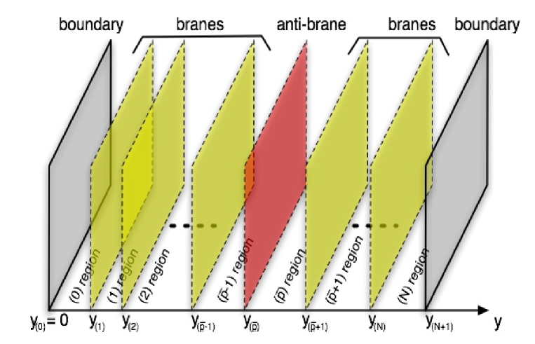
Figure 1: The brane configuration in five-dimensional heterotic M-theory

That is, the position of the $p$-th brane in the orbifold direction is determined by $y_{(p)}$, where $p=1,\dots,N$. Even though the orbifold boundaries are non-dynamical, it is convenient to introduce trivial embedding coordinates $y=y_{(0)}=0$ and $y=y_{(N+1)}=\pi\rho$ for them. For ease of notation, we also denote the embedding coordinate of the anti three-brane as $\bar{y}=y_{({\bar{p}})}$ . We will also frequently use normalized orbifold coordinates $z=y/\pi\rho\in[0,1]$ and $z_{(p)}=y_{(p)}/\pi\rho\in[0,1]$, where $p=0,\dots,N+1$, to simplify our notation.

Finally, we should briefly discuss the charges and tensions of the orbifold boundaries and branes. For this purpose, it is useful to introduce an integral basis $C^{k}$, where $k,l,\dots=1,\dots,h^{1,1}(X)$, of the second homology of the internal Calabi-Yau space $X$. Suppose that the $p$-th M five-brane, where $p=1,\dots,N$, wraps the cycle $C^{(p)}$ given by

$$C^{(p)}=\beta^{(p)}_{k}C^{k}\;.$$ (2)

Then the integer coefficients $(\beta^{(p)}_{k})$ represent the charge vector of the brane $p$. The charges on the orbifold boundaries are determined by the second Chern classes $c_{2}(X)$, $c_{2}(V_{(0)})$ and $c_{2}(V_{(N+1)})$ of the Calabi-Yau space $X$ and the two internal vector bundles $V_{(0)}$ and $V_{(N+1)}$ on the boundaries, respectively. More explicitly, we can define the charge vectors $(\beta^{(0)}_{k})$ and $(\beta^{(N+1)}_{k})$ of the two boundaries by

$$c_{2}(V_{(0)})-\frac{1}{2}c_{2}(X)=\beta^{(0)}_{k}C^{k}\;,\qquad c_{2}(V_{(N+1)})-\frac{1}{2}c_{2}(X)=\beta^{(N+1)}_{k}C^{k}\;.$$ (3)

Heterotic anomaly cancellation dictates that

$$\sum_{p=0}^{N+1}\beta^{(p)}_{k}=0$$ (4)

for each $k=1,\dots,h^{1,1}(X)$. For the orbifold boundaries and the three-branes the tensions $\tau^{(p)}_{k}$ are equal to the charges, so we have $\tau^{(p)}_{k}=\beta^{(p)}_{k}\mbox{ for }p\neq\bar{p}$. For the anti three-brane, on the other hand, tensions and charges have opposite signs, so $\tau^{({\bar{p}})}_{k}=-\beta^{({\bar{p}})}_{k}$. It should be noted that the tension of the anti three-brane is positive. In subsequent equations it will often be instructive to single out terms related to the anti three-brane and, when doing so, we will simply write the tension and charge of the anti three-brane as $\bar{\tau}_{k}\equiv\tau_{k}^{({\bar{p}})}$ and ${\bar{\beta}}_{k}\equiv\beta_{k}^{({\bar{p}})}$. It is also useful to introduce the step-functions

$$\hat{\beta}_{k}(y)=\sum_{p,y_{(p)}<y}\beta_{k}^{(p)}$$ (5)

which represent the sum of the charges to the left of a given point $y$ in the interval.

2.1 The Five-Dimensional Theory

Our starting point is the action of five-dimensional heterotic M-theory [36, 37, 38], obtained from 11-dimensional Hořava-Witten theory [49] by compactifying on a Calabi-Yau manifold $X$ in the presence of both M5 and anti-M5 branes. In this subsection, we will describe the field content of this theory and then present the action itself. Many of the detailed definitions of quantities which appear here can be found in the Appendix.

We start by describing the bulk field content, focusing on the bosonic degrees of freedom. In addition to the five-dimensional metric $g_{\alpha\beta}$, the bulk fields consist of a Kähler sector, labeled by indices $k,l,\dots=1,\dots,h^{1,1}(X)$ and a complex structure sector, labeled by indices $a,b,\dots=1,\dots,h^{2,1}(X)$ or $A,B,\dots=0,\dots,h^{2,1}(X)$. In the Kähler sector, we have $h^{1,1}(X)$ Abelian vector fields ${\cal A}_{\alpha}^{k}$ with field strengths ${\cal F}_{\alpha\beta}^{k}$ which descend from the M-theory three-form, a real scalar field $V$ which measures the Calabi-Yau volume and $h^{1,1}(X)$ metric Kähler moduli $b^{k}$ which obey the condition $d_{ijk}b^{i}b^{j}b^{k}=6$ and measure the relative size of the Calabi-Yau two-cycles. In the complex structure sector, we have $h^{2,1}(X)$ metric complex structure moduli ${\mathfrak{z}}^{a}$ and $2(h_{2,1}+1)$ scalar fields $\xi^{A}$ and $\tilde{\xi}_{B}$ which descend from the M-theory three-form. This three-form also gives rise to a five-dimensional three-form $C_{\alpha\beta\gamma}$ and its field strength $G_{\alpha\beta\gamma\delta}$. Of these bulk fields, $V$, ${\mathfrak{z}^{a}}$, $g_{\mu\nu}$, $g_{yy}$, $b^{k}$, $C_{\mu\nu y}$ and ${\cal A}^{k}_{y}$ are even under the ${\mathbb{Z}}_{2}$ action of the $S^{1}/{\mathbb{Z}}_{2}$ orbifold, while $g_{\mu y}$, $\xi^{A}$, $\tilde{\xi}_{B}$, ${\cal A}^{k}_{\mu}$, $C_{\mu\nu\gamma}$ are odd. The 11-dimensional origin of these fields is explained in Appendix A.

The bulk theory is a $d=5$, ${\cal N}=1$ supergravity and, hence, the various fields above should form the bosonic parts of five-dimensional supermultiplets. The bosonic field content of the five-dimensional supergravity multiplet consists of the five-dimensional metric $g_{\alpha\beta}$ and an Abelian gauge field, which can be identified as the linear combination $b_{k}{\cal A}_{\alpha}^{k}$. The remaining $h^{1,1}(X)-1$ vectors, together with the $h^{1,1}(X)-1$ Kähler moduli $b^{k}$, form the bosonic parts of $h^{1,1}(X)-1$ vector multiplets. The remaining scalar fields, that is, the Calabi-Yau volume modulus $V$, the dual of the three-form $C_{\alpha\beta\gamma}$, the complex structure moduli ${\mathfrak{z}}^{a}$ and the axions $\xi^{A}$, $\tilde{\xi}_{B}$ account for the bosonic parts of $h^{2,1}+1$ hypermultiplets, each of which contains four real scalars.

As usual, we have additional degrees of freedom which live on the orbifold boundaries and branes. On the four-dimensional orbifold boundaries, labeled by $p=0,N+1$, we have ${\cal N}=1$ gauge theories with gauge fields $A_{(p)\mu}$ transforming in the adjoint of the gauge groups ${\cal H}_{(p)}\subseteq E_{8}$ and gauge matter fields in ${\cal N}=1$ chiral multiplets with scalar components $C^{Ix}_{(p)}$. They transform in representations of ${\cal H}_{(p)}$ which we shall denote by $R_{(p)I}$, with $I,J,\dots$ labeling the different representations and $x,y\dots$ the states within each representation. More details on the origin and structure of the matter sector can be found in Appendix B.

The world-volume fields associated with the three-branes which descend from wrapping an M5 brane on a holomorphic (or anti-holomorphic) curve in the Calabi-Yau space are the following. The embedding coordinate (brane position) $y_{(p)}$ together with the world volume scalar $s_{(p)}$ which descends from the two-form on the M five-brane world-volume, pair together to form the bosonic content of an ${\cal N}=1$ chiral multiplet, $(y_{(p)},s_{(p)})$. In addition, we have ${\cal N}=1$ gauge multiplets with the associated field strengths denoted by $E^{u}_{(p)}$. Here $u,v\dots=1,...,g_{(p)}$, where $g_{(p)}$ is the genus of the curve $C^{(p)}$ wrapped by the $p$-th M5 brane. In general, there will be additional chiral multiplets describing the moduli space of the five brane curves and non-Abelian generalizations of the gauge field degrees of freedom when M5 branes are stacked. These are not vital to our discussion and we will not explicitly take them into account. A similar selection of four-dimensional fields appears on the anti-brane world volume.

Given this field content, the following is the bosonic part of the five-dimensional action describing Hořava-Witten theory [49] compactified on an arbitrary Calabi-Yau manifold [50, 51, 36, 37, 38] in the presence of M5 and anti-M5 branes.

$$S=-\frac{1}{2\kappa_{5}^{2}}\int d^{5}x\sqrt{-g}\left[\frac{1}{2}R+\frac{1}{4}G_{kl}(b)\partial b^{k}\partial b^{l}+\frac{1}{2}G_{kl}(b){\cal F}^{k}_{\alpha\beta}{\cal F}^{l\alpha\beta}+\frac{1}{4}V^{-2}(\partial V)^{2}+\lambda(d_{ijk}b^{i}b^{j}b^{k}-6)\right.$$

$$\left.+\frac{1}{4}{\cal K}_{a\bar{b}}({\mathfrak{z}})\partial{\mathfrak{z}}^{a}\partial\bar{{\mathfrak{z}}}^{\bar{b}}-V^{-1}(\tilde{\cal X}_{A\alpha}-\bar{M}_{AB}({\mathfrak{z}}){\cal X}_{\alpha}^{B})([\textnormal{Im}{(M({\mathfrak{z}}))}]^{-1})^{AC}(\tilde{\cal X}_{C}^{\alpha}-M_{CD}({\mathfrak{z}}){\cal X}^{D\alpha})\right.$$

$$\left.+\frac{1}{4!}V^{2}G_{\alpha\beta\gamma\delta}G^{\alpha\beta\gamma\delta}+m^{2}V^{-2}G^{kl}(b)\hat{\beta}_{k}\hat{\beta}_{l}\right]$$

$$-\frac{1}{2\kappa_{5}^{2}}\int\left(\frac{2}{3}d_{klm}{\cal A}^{k}\wedge{\cal F}^{l}\wedge{\cal F}^{m}+2G\wedge((\xi^{A}\tilde{\cal X}_{A}-\tilde{\xi}_{A}{\cal X}^{A})-2m\hat{\beta}_{k}{\cal A}^{k})\right)$$

$$-\int d^{5}x\;\delta(y)\sqrt{-h_{(0)}}\,\left[\frac{m}{\kappa_{5}^{2}}V^{-1}b^{k}\tau^{(0)}_{k}+\frac{1}{16\pi\alpha_{\textnormal{GUT}}}V\rm{tr}(F_{(0)}^{2})+G_{(0)IJ}D_{\mu}C^{Ix}_{(0)}D^{\mu}\bar{C}^{J}_{(0)x}\right.$$ (6)

$$\left.+V^{-1}G^{IJ}_{(0)}\frac{\partial W_{(0)}}{\partial C^{Ix}_{(0)}}\frac{\partial\bar{W}_{(0)}}{\partial\bar{C}^{J}_{(0)x}}+{\rm tr}(D_{(0)}^{2})\right]$$

$$-\int d^{5}x\;\delta(y-\pi\rho)\sqrt{-h_{(N+1)}}\,\left[\frac{m}{\kappa_{5}^{2}}V^{-1}b^{k}\tau^{(N+1)}_{k}+\frac{1}{16\pi\alpha_{\textnormal{GUT}}}V{\rm tr}(F_{(N+1)}^{2})\right.$$

$$\left.+G_{(N+1)IJ}D_{\mu}C^{Ix}_{(N+1)}D^{\mu}\bar{C}^{J}_{(N+1)x}+V^{-1}G^{IJ}_{(N+1)}\frac{\partial W_{(N+1)}}{\partial C^{Ix}_{(N+1)}}\frac{\partial\bar{W}_{(N+1)}}{\partial\bar{C}^{J}_{(N+1)x}}+{\rm tr}(D_{(N+1)}^{2})\right]$$

$$-\frac{1}{2\kappa_{5}^{2}}\int d^{5}x\;\left\{\sum_{p=1}^{N}(\delta(y-y_{(p)})+\delta(y+y_{(p)}))\sqrt{-h_{(p)}}\,\left[mV^{-1}\tau^{(p)}_{k}b^{k}+\frac{2m(n_{(p)}^{k}\tau^{(p)}_{k})^{2}}{V(\tau^{(p)}_{l}b^{l})}j_{{(p)}\mu}j^{\mu}_{(p)}\right.\right.$$

$$\left.\left.+[\textnormal{Im}{\Pi}]_{{(p)}uw}E^{u}_{{(p)}\mu\nu}E^{w\mu\nu}_{(p)}\right]-4m\hat{C}_{(p)}\wedge\tau^{(p)}_{k}d(n^{k}_{(p)}s_{(p)})-2[\textnormal{Re}{\Pi}]_{(p)uw}E^{u}_{(p)}\wedge E^{w}_{(p)}\right\}$$

Let us briefly discuss the various quantities in this action. In the previous section, we defined the charges $\beta^{(p)}_{k}$, the tensions $\tau^{(p)}_{k}$ and the charge step-functions $\hat{\beta}_{k}$. To introduce the remaining objects, we start with the bulk theory, the first part of the above action. Of course, $\kappa_{5}$ is the five-dimensional Planck constant, related to its 11-dimensional counterpart $\kappa_{11}$ by $\kappa_{5}^{2}=\kappa_{11}^{2}/v$ where $v$ is the Calabi-Yau reference volume. The constant $m$ is given by

$$m=\frac{2\pi}{v^{\frac{2}{3}}}\left(\frac{\kappa_{11}}{4\pi}\right)^{\frac{2}{3}}$$ (7)

and represents a reference mass scale of the Calabi-Yau space. The quantity $\lambda$ is a Lagrange multiplier enforcing the constraint on the $b^{k}$ moduli. The Kähler and complex structure moduli metrics $G_{kl}$ and ${\cal K}_{a\bar{b}}$ are defined in Appendix A. A definition of the Calabi-Yau intersection numbers $d_{ijk}$ and the special geometry quantity $M_{AB}$ can also be found in this Appendix. The various bulk form field strengths are defined in the usual way as $G=dC$, ${\cal F}^{k}=d{\cal A}^{k}$ and ${\cal X_{A}}=d\xi_{A}$, $\tilde{\cal X}_{A}=d\tilde{\xi}_{A}$ away from the boundaries, but are subject to boundary source terms specified by the relations

$$(dG)_{y\mu\nu\gamma\rho} = -4\kappa_{5}^{2}(J^{(0)}_{4\mu\nu\gamma\rho}\delta(y)+J^{(N+1)}_{4\mu\nu\gamma\rho}\delta(y-\pi\rho))$$ (8)

$$(d{\cal F}^{k})_{y\mu\nu} = -4\kappa^{2}_{5}(J^{(0)k}_{2\mu\nu}\delta(y)+J^{(N+1)k}_{2\mu\nu}\delta(y-\pi\rho))$$ (9)

$$(d{\cal X}^{A}{\cal G}_{A}-d\tilde{{\cal X}}_{B}{\cal Z}^{B})_{y\mu} = -4\kappa^{2}_{5}(J^{(0)}_{1\mu}\delta(y)+J^{(N+1)}_{1\mu}\delta(y-\pi\rho))$$ (10)

where

$$J^{(p)}_{4\mu\nu\gamma\rho} = \frac{1}{16\pi\alpha_{\textnormal{ GUT}}}\textnormal{tr}(F_{(p)}\wedge F_{(p)})_{\mu\nu\gamma\rho}$$ (11)

$$J^{(p)k}_{2\mu\nu} = -i\sum_{I,J}\Gamma^{k}_{(p)IJ}(D_{\mu}C_{(p)}^{Ix}D_{\nu}\bar{C}_{(p)x}^{J}-D_{\mu}\bar{C}_{(p)x}^{I}D_{\nu}C_{(p)}^{Jx})$$ (12)

$$J^{(p)}_{1\mu} = \frac{e^{-{\cal K}}}{2V}\sum_{I,J,K}\lambda_{IJK}f_{xyz}^{(IJK)}C_{(p)}^{Ix}C_{(p)}^{Jy}D_{\mu}C_{(p)}^{Kz}$$ (13)

for $p=0,N+1$. The various matter field objects in these sources are defined in Appendix B. One important observation from these Bianchi identities is that the three-branes and anti three-branes do not contribute any source terms. This fact will be crucial in our later analysis. The second and third parts of the above action are the theories on the two orbifold boundaries respectively. They are written in terms of the matter field Kähler metrics $G_{(p)MN}$, the matter field superpotentials $W_{(p)}$ and the D-terms $D_{(p)}$. Definitions for these quantities can also be found in Appendix B. The (reference) gauge coupling constant $\alpha_{\textnormal{GUT}}$ is given by $\alpha_{\textnormal{GUT}}=(4\pi\kappa_{11}^{2})^{2/3}/v$.

We move on to discuss the three-brane world volume theories, the last part of the above action. The quantities $n_{(p)}^{k}=\beta^{(p)}_{k}/\sum_{l=1}^{N}{\beta^{(p)2}_{l}}$ are a normalized version of the three-brane charges and the axionic currents $j_{(p)\mu}$ are defined by

$$j_{(p)\mu}=\frac{\beta^{(p)}_{k}}{n_{(p)}^{l}\beta^{(p)}_{l}}(d(n^{k}_{(p)}s_{(p)})-{\hat{\cal A}}^{k}_{(p)})_{\mu}\;,$$ (14)

where $\hat{C}_{(p)}$ and ${\hat{\cal A}}^{k}_{(p)}$ denote the pull-backs of the bulk forms $C$ and ${\cal A}^{k}$ to the $p$-th brane. The gauge kinetic functions $\Pi_{(p)uv}$ of the three-brane gauge fields are defined in Appendix C.

Finally, we need to mention that the induced metrics $h_{(p)\mu\nu}$ on the orbifold boundaries and branes are explicitly given by

$$h_{(p)\mu\nu}=g_{\mu\nu}+g_{\mu y}\partial_{\nu}y_{(p)}+g_{y\nu}\partial_{\mu}y_{(p)}+g_{yy}\partial_{\mu}y_{(p)}\partial_{\nu}y_{(p)}\;,$$ (15)

where the embedding (1) has been used. Recall that the boundaries are non-dynamical with associated static embeddings $y_{(0)}=0$ and $y_{(N+1)}=\pi\rho$. Hence, the induced boundary metrics $h_{(0)}$ and $h_{(N+1)}$ are simply equal to $g_{\mu\nu}$, the four-dimensional part of the bulk space-time metric. The action described in this section must be supplemented by the usual Gibbons-Hawking boundary terms. A careful analysis reveals that form-field boundary terms are not required in this case.

Having described the five-dimensional theory, our starting point, we proceed in the next section to discuss the appropriate reduction ansatz in the presence of anti-branes. The dimensional reduction to four-dimensions will be performed in section 4.

3 The Five-Dimensional Domain Wall with Anti-Branes

In this section, we illustrate the main features of the five-dimensional reduction ansatz in the context of a simple scalar field toy model. We will then explicitly work out the essential part of this reduction ansatz, the five-dimensional non-supersymmetric domain wall. This is a generalization of the BPS domain wall solution of Ref. [36, 37] and includes the back-reaction effects of the anti three-brane.

The key new point for us will be to discover how the back-reaction on the bulk fields due to the presence of the branes and, in particular, the anti-brane is taken into account in the reduction ansatz. While this is technically complicated for five-dimensional heterotic M-theory, the basic ideas can be explained in a simple setting. Before dealing with the full problem, we will, therefore, discuss a scalar field toy model [52] to illustrate the key features involved. The structure of space-time and branes for this model is precisely as described above and illustrated in Fig. 1. The action is given by

$$S\sim\int d^{5}x\,\left[\partial_{\alpha}\Phi\partial^{\alpha}\Phi-\delta(y)\,S_{(0)}\Phi-\delta(y-\pi\rho)\,S_{(N+1)}\Phi-\sum_{p=1}^{N}(\delta(y-y_{(p)})+\delta(y+y_{(p)}))\,S_{(p)}\Phi\right]\;,$$ (16)

where $S_{(p)}$ are sources on the boundaries and branes (which can depend on other fields) and $\Phi$ is a ${\mathbb{Z}}_{2}$ even scalar field. What we want to discuss in this model is the warped background solution which arises due to the presence of the source terms and the four-dimensional effective theory associated with it. To this end, it is useful to split the scalar field as $\Phi=\phi+\phi_{0}$, where $\phi_{0}$ is a function of the four-dimensional coordinates only and is the quantity that will become the modulus associated with this degree of freedom in the four-dimensional effective theory. On the other hand, $\phi$ represents a function of all five coordinates and contains the warping of the background due to the presence of sources terms. To uniquely define this splitting of $\Phi$, we require that the orbifold average $<\phi>$ of $\phi$ vanishes. This condition implies a specific choice of coordinates on field space in the resulting four-dimensional effective theory. This choice is particularly useful in finding a clean form for the resulting action, as we will see explicitly throughout this paper.

The field equation for $\Phi$, valid in each bulk region indicated in Fig. 1, then reads

$$\Box_{4}\phi_{0}+\Box_{4}\phi+D_{y}^{2}\phi=0\;.$$ (17)

In addition, $\Phi$ is subject to boundary conditions at the edge of each region due to the presence of the sources. For the two orbifold boundaries, these take the form

$$D_{y}\phi|_{y=0}=-S_{(0)}\;,\qquad D_{y}\phi|_{y=\pi\rho}=+S_{(N+1)}$$ (18)

while, for the branes, we have

$$-D_{y}\phi|_{y=y_{(p)}+}+D_{y}\phi|_{y=y_{(p)}-}=S_{(p)}\;,$$ (19)

where $p=1,\dots,N$. The subscript “$y=y_{(p)}+$” (“$y=y_{(p)}-$”) indicates that the relevant quantity should be evaluated approaching the $p$-th brane from the right (left).

We can now take an average of the equation of motion (17) over the orbifold. Using $<\phi>=0$ and the “boundary conditions” (18) and (19), we obtain

$$\Box_{4}\phi_{0}+\sum_{p}S_{(p)}=0\;.$$ (20)

This relation may then be used to eliminate $\phi_{0}$ in (17) to obtain an equation purely for the warping

$$\Box_{4}\phi+D^{2}_{y}\phi=\sum_{p}S_{(p)}.$$ (21)

To pursue the analysis further, we need to know something about the various approximations, and associated expansions, which are made in deriving four-dimensional heterotic M-theory, some of which have already been implicit in our analysis. Two expansions in particular are of central importance at this point. The first of these is simply the usual expansion in four-dimensional derivatives which is always made in defining such an effective theory; in other words, the four-dimensional fields are assumed to be slowly varying relative to the structure in the internal dimensions. The second expansion which we need is in terms of a small parameter $\epsilon_{S}$, which controls the size of the source terms. We will meet this quantity explicitly soon, so let us just state this to be true for now. The zero mode $\phi_{0}$ is a quantity independent of the warping and is, therefore, zeroth order in the $\epsilon_{S}$ expansion. By contrast, $\phi$ is precisely the quantity which presents the warping and so is first order $\epsilon_{S}$. Looking at (21) which determines the warping, we see that the first term is both first order in $\epsilon_{S}$ and second order in four-dimensional derivatives whereas the remaining terms are simply first order in $\epsilon_{S}$. We may therefore, in a controlled approximation, ignore the first term in (21). This results in the following equation for the warping

$$D_{y}^{2}\phi=\sum_{p}S_{(p)}.$$ (22)

Thus, in the end, we need to solve the system of bulk equations and boundary conditions given by (18), (19) and (22). Before moving on to the full calculation, we qualitatively describe such an analysis in various cases by transferring the insight from the above toy example to heterotic M-theory. We start with heterotic M-theory in the absence of anti-branes and proceed to a discussion of the back-reaction of such objects when they are included in the vacuum.

a) Zeroth order in sources

When all of the sources are set to zero, the warping equation (22) becomes simply $D^{2}_{y}\phi=0$. Since $\phi$ must be continuous around the orbifold this, in combination with the condition $<\phi>=0$, results in $\phi=0$. For five-dimensional heterotic M-theory, this implies that the zeroth order vacuum is simply five-dimensional Minkowski space.

b) The standard heterotic vacuum

In the case of a heterotic vacuum involving only orbifold fixed planes and three-branes (but no anti three-branes), the sources $S_{(p)}$ are represented by the tension terms of the branes and boundaries and they obey a particularly useful relation. Since the objects involved are all BPS, their tensions are equal to their charges. The charges, on the other hand, have to sum to zero as a result of the heterotic anomaly cancellation condition (4). Thus, we have for such compactifications that $\sum_{p}S_{(p)}=0$ and, as in the previous case, the equation for the warping (22) reduces to $D^{2}_{y}\phi=0$. The boundary conditions (18), (19) are no longer trivial however. Thus, the only solution for $\phi$ is a function linear in each region of Fig. 1, with kinks at the boundary and brane positions. The slope in each region is chosen such that equations (18), (19) are obeyed. The fact that the source terms sum to zero ensures that we indeed have a globally well-defined solution. This situation corresponds to the “Universe as a Domain Wall” vacuum of heterotic M-theory [36, 37].

c) Matter fluctuation induced warping in the case without anti-branes

We have just seen that the vacuum of heterotic M-theory is linearly warped if only tension sources of BPS objects are considered. However, even in the absence of anti-branes this is not the full story [51, 52]. For example, fluctuations of matter fields on the orbifold fixed planes lead to additional source terms. Since fields on the various orbifold boundaries and branes fluctuate independently, these sources do not, in general, obey the sum rule $\sum_{p}S_{(p)}=0$. As a result, we obtain warping quadratic in the orbifold coordinate $y$. This is typical of heterotic M-theory: any change to the source terms away from the case of “pure tension” results in quadratic contributions to the warping.

d) The back-reaction of anti-branes in heterotic M-theory

We are now in a position to understand how the presence of an anti-brane in the bulk of heterotic M-theory changes the warping. In other words, we can now see how to calculate the back-reaction due to the presence of the anti-brane. The relevant source terms - the tensions of the orbifold boundaries, the three-branes and the anti three-branes - are very similar to those for the usual BPS situation described in b). While the charges of these objects still add up to zero, the same can no longer be said for the tensions since the anti three-brane tension is minus its charge. Hence, the bulk equation (22) contains a non-vanishing source term $\sum_{p}S_{(p)}\neq 0$ due to the tension terms. It is clear from the discussion in c) that this implies a quadratic term in the warping. More precisely, using the usual linear warping we can ensure that all boundary conditions, except the one at the right boundary $y=\pi\rho$, are satisfied. Since the sum of the sources no longer vanishes, the linear warping does not match the final boundary condition at $y=\pi\rho$. We therefore add a quadratic piece to the warping. This does not change the kink structure of the solution across the branes, but does allow one to satisfy the boundary condition at $y=\pi\rho$. In addition, when we examine the bulk equation (22), we find that this additional quadratic warping is precisely what is required to balance the source term now present on the right-hand side.

With the insight from this toy model, we now proceed to analyze full five-dimensional heterotic M-theory. In the remainder of this section, we focus on the warping caused by the tension terms. This will lead us to a generalization of the heterotic domain wall vacuum, valid in the presence of an anti-brane. The additional warping due to fluctuations of localized fields is presented in Appendix D.

The only bulk fields involved in the generalized domain wall solution are the ones which couple to the tension terms in the action (2.1). They are the metric $g_{\alpha\beta}$, the volume modulus $V$ and the Kähler moduli $b^{k}$. We start with the usual metric ansatz involving the four dimensional metric $g_{4\mu\nu}$.

$$ds^{2}_{5} = a^{2}(y,x^{\mu})g_{4\mu\nu}dx^{\mu}dx^{\nu}+b^{2}(y,x^{\mu})dy^{2}$$ (23)

$$V = V(y,x^{\mu})$$ (24)

$$b^{k} = b^{k}(y,x^{\mu})\;.$$ (25)

In writing our result, it is useful to introduce the following function which encodes the standard linear warping of heterotic M-theory and averages to zero over the orbifold

$$h_{(p)k}(z)=\sum^{p}_{q=0}\tau^{(q)}_{k}(z-z_{(q)})-\frac{1}{2}\sum_{q=0}^{N+1}\tau^{(q)}_{k}z_{(q)}(z_{(q)}-2)-\delta_{k}\;,$$ (26)

where we have defined the difference of anti three-brane tension and charge as

$$\delta_{k}=\frac{1}{2}(\bar{\tau}_{k}-\bar{\beta}_{k})=-\bar{\beta}_{k}\;.$$ (27)

In the following, whenever we want to consider the supersymmetric limit of our results, we can “switch off” the effect of the anti three-brane by formally setting $\delta^{k}\rightarrow 0$. Recall that the sub-script “$(p)$” indicates that the domain of the function $h_{(p)k}$ is $z\in[z_{(p)},z_{(p+1)}]$, that is, the region to the right of the $p$-th brane. Using the Einstein equation and the equations of motion for $V$ and $b^{k}$ derived from the action (6), together with the above ansatz, gives the following solution for the warping

$$\frac{a_{(p)}}{a_{0}} = 1-\epsilon_{0}\frac{b_{0}}{3V_{0}}b_{0}^{k}\left[h_{(p)k}-\delta_{k}\left(z^{2}-\frac{1}{3}\right)\right]$$ (28)

$$\frac{V_{(p)}}{V_{0}} = 1-2\epsilon_{0}\frac{b_{0}}{V_{0}}b_{0}^{k}\left[h_{(p)k}-\delta_{k}\left(z^{2}-\frac{1}{3}\right)\right]$$ (29)

$$b_{(p)}^{k} = b_{0}^{k}+2\epsilon_{0}\frac{b_{0}}{V_{0}}\left[\left(h_{(p)}^{k}-\frac{1}{3}h_{(p)l}b_{0}^{k}b_{0}^{l}\right)-\left(\delta^{k}-\frac{1}{3}\delta_{l}b_{0}^{k}b_{0}^{l}\right)\left(z^{2}-\frac{1}{3}\right)\right].$$ (30)

We remind the reader of the relationship $z=y/{\pi\rho}$. In these expressions, $a_{0}$, $b_{0}$, $V_{0}$ and $b_{0}^{k}$ are four-dimensional moduli fields. Note that due to our convention of zero average warping, these moduli are precisely the orbifold average of the corresponding five-dimensional fields. For example $V_{0}=<V>$ is the orbifold average of the Calabi-Yau volume and $b_{0}=<b>$ is the average orbifold radius. We observe that the warping in the above solution is indeed proportional to the strong-coupling expansion parameter $\epsilon_{S}$, defined by

$$\epsilon_{S}=\epsilon_{0}\frac{b_{0}}{V_{0}}\;,\qquad\epsilon_{0}=\pi\rho m$$ (31)

as promised. Note using (7) that $\epsilon_{S}\propto\kappa_{11}^{2/3}$. Our result is valid as long as $\epsilon_{S}\ll 1$, since we have neglected warping terms of order $\epsilon_{S}^{2}$ and higher. The structure of the ${\cal O}(\epsilon_{S})$ warping terms is as qualitatively described earlier. In the supersymmetric limit, $\delta^{k}\rightarrow 0$, we recover the linear warping of the BPS domain wall encoded in the functions $h_{(p)k}$. On the other hand, the terms proportional to $\delta^{k}$, which are caused by the presence of the anti three-brane, represent quadratic warping. The observant reader will note that we have not given an expression for the warping of the metric coefficient $b$. This is because this $y$ dependence amounts to a coordinate choice and, as such, is not needed in the calculation of the four dimensional effective action.

A specific example of the warping of the Calabi-Yau volume modulus $V$ is plotted in Fig. 2. This example shows that the presence of an anti-brane can change the warping substantially. As is clear from the action (2.1), the volume $V$ at the boundaries $z=0,1$ determines the value of the boundary gauge couplings. In particular, the BPS configuration in Fig. 2 (dashed, red curve) corresponds to weak coupling at $z=0$ and strong coupling at $z=1$. As is evident from the Figure, this behavior can be reversed in the presence of the anti-brane (solid, green curve).

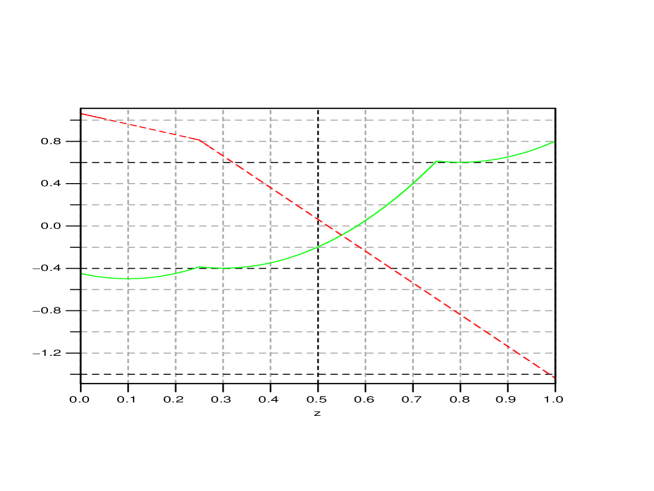
Figure 2: Warping of the Calabi-Yau volume modulus V (bracket on the RHS of (29)), assuming $h^{1,1}(X)=1$. The dashed, red curve corresponds to a BPS configuration with one brane at $z=1/4$ and charge vector $(\beta^{(p)})=(1,2,-3)$. The solid, green curve describes a situation with one brane at $z=1/4$, one anti-brane at $z=3/4$ and charge vector $(\beta^{(p)})=(1,2,-5,2)$. It can be obtained from the previous BPS configuration by “pulling” an anti-brane with charge $-5$ off the boundary at $z=1$.

4 Heterotic M-Theory with Anti-Branes in Four Dimensions

In this section, we construct the four-dimensional effective theory describing heterotic M-theory when anti-branes are present in the vacuum, focusing on terms that are zeroth and first order in $\kappa_{11}^{\frac{2}{3}}$. In the next section, we will present some terms of order $\kappa_{11}^{\frac{4}{3}}$ which can be reliably calculated, concentrating on those which will be important in applications to moduli stabilization.

4.1 The Reduction Ansatz and Zero Modes

We start by discussing the zero modes and the reduction ansatz used in the rest of the paper. The essential part of the ansatz is the non-supersymmetric domain wall, introduced in the previous section. Let us focus on this part of the ansatz for now. We will discuss additional terms due to fluctuations of localized fields later. For the five-dimensional metric, recall (23),

$$ds_{5}^{2}=a^{2}(y)g_{4\mu\nu}dx^{\mu}dx^{\nu}+b^{2}(y)dy^{2}\;,$$ (32)

where the warping $a(y)$ is given in (28). The domain wall also involves non-trivial warping for the volume modulus $V$ and the Kähler moduli $b^{k}$, as given in (29) and (30). In addition to the four-dimensional metric, the complete solution contains the moduli $V_{0}$, $a_{0}$, $b_{0}$ and $b_{0}^{k}$, which are four-dimensional fields. Recall that $V_{0}$ is the orbifold average of the Calabi-Yau volume and $b_{0}$ is the average radius of the orbifold and we will frequently write

$$b_{0}=e^{\beta}\;,\qquad V_{0}=e^{\phi}\;.$$ (33)

The modulus $a_{0}$ is really the four-dimensional scale factor and is redundant given that we have already introduced a full four-dimensional metric into our ansatz. However, it can be conveniently used to bring the four-dimensional Einstein-Hilbert term into canonical form, which is achieved by fixing $a_{0}^{2}=1/b_{0}$. Further zero modes arise from the ${\mathbb{Z}}_{2}$ even components of the other bulk fields. Specifically, these are the zero modes of the complex structure moduli ${\mathfrak{z}}^{a}$, the axions $\chi^{k}={\cal A}^{k}_{y}$ and the two-form $B_{\mu\nu}=C_{y\mu\nu}$ with field strength $H_{\mu\nu\rho}=G_{y\mu\nu\rho}$, which we dualize to a scalar $\sigma$, as usual. Note, in particular, that the fields $\xi^{A}$ and $\tilde{\xi}_{A}$ are ${\mathbb{Z}}_{2}$ odd and do not give rise to zero modes. However, the $y$-components ${\cal X}_{y}$ and $\tilde{\cal X}_{y}$ of their field strengths are ${\mathbb{Z}}_{2}$ even and having these components non-zero corresponds to switching on $H$-flux from a 10-dimensional heterotic view point. Flux in the context of heterotic models with anti-branes will be considered in Ref. [48] but, for the purposes of this paper, we simply set ${\cal X}_{y}$ and $\tilde{\cal X}_{y}$ to zero. In the following, we will drop the “$0$”sub-script from the four-dimensional fields for ease of notation, for example, writing $b^{k}_{0}$ as $b^{k}$.

Fields localized on the orbifold boundaries and the branes are, of course, already four-dimensional and are simply retained in the four-dimensional effective theory. In particular, for the four-dimensional position moduli of the branes we will use the normalized fields $z_{(p)}\in[0,1]$ and, in particular, $\bar{z}$ for the anti three-brane. It is useful to normalize the associated brane axion fields $s_{(p)}$ accordingly by defining $\nu_{(p)}=s_{(p)}/\pi\rho$. We also have the pull-backs of bulk fields appearing on the boundaries and branes. These have to be computed by applying the embedding (1) to the reduction ansatz for the bulk fields. For example, for the induced metrics on the branes we have

$$\sqrt{-h_{(p)}}=a^{4}\sqrt{-g_{4}}\left(1+\frac{b^{2}}{2a^{2}}\partial_{\mu}y_{(p)}\partial^{\mu}y_{(p)}\right)\;.$$ (34)

As discussed earlier, fluctuations of localized fields give rise to additional warping contributions of the bulk fields. These must be integrated out to arrive at the correct effective action [51, 52]. It turns out that, to order $\kappa_{11}^{\frac{2}{3}}$, these effects are only relevant for the bulk anti-symmetric tensor fields whose warping is induced by the Bianchi identities (8)–(10). The solutions to these Bianchi identities (and the associated equations of motion) in the presence of fluctuating boundary fields are discussed in Appendix D.

We shall present our results, specified order by order in the $\kappa_{11}^{\frac{2}{3}}$ expansion parameter of Hořava-Witten theory. This parameter determines the computational complexity involved in obtaining the relevant parts of the action. Thus the discussion of how to obtain the second order pieces below is more involved than that describing the first order results. It is useful, therefore, to separate them. However, when applying these results the reader should keep in mind that the correct expansion parameter to consider in four dimensions is $\epsilon_{S}$. Thus all terms up to a given order in this parameter should be kept. In particular, when working to first order in $\epsilon_{S}$ the threshold corrections to the gauge kinetic functions and matter field terms, which are second order in $\kappa_{11}^{\frac{2}{3}}$, must be included.

There is a simple way in which the order in $\epsilon_{S}$ or $\kappa_{11}^{\frac{2}{3}}$ of any term appearing in the following can be ascertained.

• The order in $\epsilon_{S}$ of any term can be found by counting the number of powers of $\epsilon_{0}$ which are present.

• The order in $\kappa_{11}^{\frac{2}{3}}$ of any term can be determined by counting the number of powers of $\epsilon_{0}$ which are present and then adding one power if the term contains boundary gauge or matter fields. This rule is a consequence of a rescaling which must be performed to obtain standard kinetic terms for these fields.

Having forewarned the reader of this subtlety, we now present our results.

4.2 Zeroth and First Order Result for the Four-Dimensional Effective Theory

Collecting various terms, we find the following bosonic four-dimensional effective action of heterotic M-theory in the presence of an arbitrary number of M five-branes and a single anti M five-brane. This result is valid up to first order in $\kappa_{11}^{\frac{2}{3}}$ and second order in four-dimensional derivatives. We find that

$$S=S_{\delta^{0}}^{(0,1)}+S_{\delta^{1}}^{(1)},$$ (35)

where the subscript indicates that $S_{\delta^{0}}^{(0,1)}$ and $S_{\delta^{1}}^{(1)}$ contain terms independent of the parameters $\delta_{k}$ and linear in $\delta_{k}$ respectively. Similarly, the superscript implies that $S_{\delta^{0}}^{(0,1)}$ has both zeroth and first order terms in $\kappa_{11}^{\frac{2}{3}}$ whereas all terms in $S_{\delta^{1}}^{(1)}$ are of order $\kappa_{11}^{\frac{2}{3}}$. The first action in (35) is given by

$$S_{\delta^{0}}^{(0,1)}=S_{4}^{\textnormal{moduli}}+S_{4}^{\textnormal{gauge}}+S_{4}^{\textnormal{matter}},$$ (36)

with

$$S_{4}^{\textnormal{moduli}} = -\frac{1}{2\kappa^{2}_{4}}\int d^{4}x\sqrt{-g_{4}}\,\left[\frac{1}{2}R_{4}+\frac{3}{4}(\partial\beta)^{2}+\frac{1}{4}(\partial\phi)^{2}+\frac{1}{4}e^{-2\phi}(\partial\sigma)^{2}+\frac{1}{4}G_{kl}\partial b^{k}\partial b^{l}+e^{-2\beta}G_{kl}\partial\chi^{k}\partial\chi^{l}\right.$$

$$\left.+\frac{1}{4}{\cal K}_{a\bar{b}}({\mathfrak{z}})\partial{\mathfrak{z}}^{a}\partial\bar{{\mathfrak{z}}}^{\bar{b}}+2\epsilon_{0}\sum_{p=1}^{N}\tau^{(p)}_{k}z_{(p)}e^{-2\phi}\partial\sigma\partial(n_{(p)}^{k}\nu_{(p)})+\frac{\epsilon_{0}}{2}\sum_{p=1}^{N}b^{k}\tau^{(p)}_{k}e^{\beta-\phi}(\partial z_{(p)})^{2}\right.$$

$$\left.+2\epsilon_{0}\sum_{p=1}^{N}\frac{\tau^{(p)}_{l}\tau^{(p)}_{k}}{\tau^{(p)}_{m}b^{m}}e^{-\phi-\beta}\left(\chi^{l}\chi^{k}(\partial z_{(p)})^{2}-2\chi^{k}\partial(n_{(p)}^{l}\nu_{(p)})\partial z_{(p)}+\partial(n_{(p)}^{k}\nu_{(p)})\partial(n^{l}_{(p)}\nu_{(p)})\right)\right.$$

$$\qquad\qquad\qquad\qquad\left.+\lambda(d_{ijk}b^{i}b^{j}b^{k}-6)\right]$$

$$S_{4}^{\textnormal{gauge}} = -\frac{1}{16\pi\alpha_{\textnormal{GUT}}}\int d^{4}x\sqrt{-g_{4}}\,\left[e^{\phi}\left(\textrm{tr}F_{(0)}^{2}+\textrm{tr}F_{(N+1)}^{2}\right)-\frac{1}{2}\sigma\epsilon_{\mu\nu\rho\gamma}\left(F^{\mu\nu}_{(0)}F^{\rho\gamma}_{(0)}+F^{\mu\nu}_{(N+1)}F^{\rho\gamma}_{(N+1)}\right)\right.$$

$$\left.\qquad\qquad\qquad\qquad\qquad+\sum_{p=1}^{N}\left([\textnormal{Im}{\Pi}]_{(p)uw}E^{u}_{(p)}E^{w}_{(p)}-\frac{1}{2}[\textnormal{Re}{\Pi}]_{(p)uw}\epsilon_{\mu\nu\rho\gamma}E^{u\mu\nu}_{(p)}E^{w\rho\gamma}_{(p)}\right)\right]$$

$$S_{4}^{\textnormal{matter}} = -\int d^{4}x\sqrt{-g_{4}}\,\sum_{p=0,N+1}\left[\frac{1}{2}\left(e^{-\beta}G_{(p)MN}DC_{(p)}^{Mx}D\bar{C}_{(p)x}^{N}-2e^{-2\beta}G_{kl}\omega^{(p)k}_{1\mu}\partial^{\mu}\chi^{l}\right.\right.$$

$$\left.\left.\qquad\qquad\qquad\qquad\qquad+e^{-\phi-2\beta}G_{(p)}^{MN}\frac{\partial W_{(p)}}{\partial C^{Mx}_{(p)}}\frac{\partial\bar{W}_{(p)}}{\partial\bar{C}^{M}_{(p)x}}+e^{-2\beta}{\rm tr}(D^{2}_{(p)})\right)\right]$$

Here, $\kappa_{4}$ is the four-dimensional Planck constant which is related to its 11-dimensional and 5-dimensional counterparts by $\kappa_{4}^{2}=\kappa_{11}^{2}/\pi\rho v=\kappa_{5}^{2}/\pi\rho$, where $v$ is the Calabi-Yau reference volume and $\pi\rho$ is the interval length. We remind the reader that, in terms of quantities appearing elsewhere in this paper, $z_{(p)}=y_{(p)}/\pi\rho$, $\nu_{(p)}=s_{(p)}/\pi\rho$, $\phi=\ln V_{0}$, $\beta=\ln b_{0}$ and $\sigma$ is the dual of $H_{\mu\nu\rho}$. The one-forms $\omega^{(p)k}_{1\mu}$ in the matter field part of the above action are the Chern-Simons forms associated to the currents (12), that is, $d\omega^{(p)k}_{1}=J^{(p)k}_{2}$. Finally, the functions $W_{(p)}$ are given by (102) in Appendix B. The second action in (35) is much simpler and found to be

$$S_{\delta^{1}}^{(1)}=-\frac{1}{2\kappa^{2}_{4}}\int d^{4}x\sqrt{-g_{4}}\,\left[\frac{2\epsilon_{0}}{(\pi\rho)^{2}}e^{-\phi-2\beta}b^{k}\delta_{k}\right]$$ (40)

Recall that the quantities $\delta_{k}$, defined in (27), represent the differences of the tensions and charges of the anti three-brane. The complete action (35), in fact, remains valid if one replaces an arbitrary number of branes with anti-branes. Then $\delta_{k}$ should be interpreted as the sum of all anti-brane tensions minus the sum of all anti-brane charges all divided by two.

Significant results can be gleaned merely by inspecting this action.

• First notice how close the action is, at this order, to the ${\cal N}=1$ supersymmetric result. Recall that formally switching off the supersymmetry-breaking effect of the anti-brane is achieved by setting $\delta_{k}\rightarrow 0$. It follows that the $S_{\delta^{0}}^{(0,1)}$ portion of the action is identical to the bosonic part of the usual ${\cal N}=1$ supersymmetric theory [51, 53, 54, 38]. In particular, the kinetic term of the anti-brane’s position modulus, which appears in $S_{\delta^{0}}^{(0,1)}$, is identical to that of a brane of the same tension. Indeed, if we define the scalar components of superfields in the standard way [38] by

  $$S = e^{\phi}+\epsilon_{0}e^{\beta}\sum_{p=1}^{N}\,(\tau^{(p)}_{k}b^{k})z_{(p)}^{2}+i\left(\sigma+2\epsilon_{0}\sum_{p=1}^{N}\tau_{k}^{(p)}\chi^{k}z_{(p)}^{2}\right)$$ (41)

  $$= e^{\phi}+i\sigma+\epsilon_{0}\sum_{p=1}^{N}\tau_{k}^{(p)}z_{(p)}^{2}T^{k}$$ (42)

  $$T^{k} = e^{\beta}b^{k}+2i\chi^{k}$$ (43)

  $$Z_{(p)} = \tau_{k}^{(p)}b^{k}e^{\beta}z_{(p)}+2i\tau_{k}^{(p)}(-n^{k}_{(p)}\nu_{(p)}+\chi^{k}z_{(p)})$$ (44)

  $$= z_{(p)}\tau^{(p)}_{k}T^{k}-2i\tau_{k}^{(p)}n^{k}_{(p)}\nu_{(p)},\,$$ (45)

  then $S_{\delta^{0}}^{(0,1)}$ is reproduced as the bosonic part of the ${\cal N}=1$ supersymmetric theory with Kähler potential

  $$\kappa_{4}^{2}\,K_{\rm scalar}=K_{D}+K_{T}+{\cal K}+K_{\rm matter}\;,$$ (46)

  where

  $$K_{D} = -{\rm ln}\left[S+\bar{S}-\epsilon_{0}\sum_{p=1}^{N}\frac{(Z_{(p)}+\bar{Z}_{(p)})^{2}}{\tau_{k}^{(p)}(T^{k}+\bar{T}^{k})}\right]\,,$$ (47)

  $$K_{T} = -{\rm ln}\left[\frac{1}{48}d_{klm}(T^{k}+\bar{T}^{k})(T^{l}+\bar{T}^{l})(T^{m}+\bar{T}^{m})\right]$$ (48)

  $${\cal K}({\mathfrak{z}}) = -\mbox{ln}\left[2i({\mathcal{G}}-\bar{{\mathcal{G}}})-i(\mathfrak{z}^{p}-\bar{\mathfrak{z}}^{p})\left(\frac{\partial\mathcal{G}}{\partial\mathfrak{z}^{p}}+\frac{\partial\bar{\mathcal{G}}}{\partial\bar{\mathfrak{z}}^{p}}\right)\right]$$ (49)

  $$K_{\rm matter} = e^{K_{T}/3}\sum_{p=0,N+1}G_{(p)MN}C^{Mx}_{(p)}\bar{C}_{(p)x}^{N}\;,$$ (50)

  with superpotential for the matter chiral multiplets given by

  $$W_{(p)}=\sqrt{4\pi\alpha_{\rm GUT}}\sum_{I,J,K}\lambda_{IJK}f_{xyz}^{(IJK)}C_{(p)}^{Ix}C_{(p)}^{Jy}C_{(p)}^{Kz}$$ (51)

  and with gauge kinetic functions

  $$f_{(p)} = S\;,\quad p=0,N+1$$ (52)

  $$f_{(p)uv} = \Pi_{(p)uv}\;,\quad p=1,\dots,N\;.$$ (53)

  This is exactly the standard result for heterotic M-theory without anti-branes [38]. Note that the superpotential $W_{(p)}$ leads to a non-vanishing potential energy term for the matter scalars $C_{(p)}^{Ix}$. However, the matter independent potential energy of the dilaton and moduli fields vanishes in the formal limit $\delta_{k}\rightarrow 0$, as it must.

• Since $S_{\delta^{1}}^{(1)}$ in (40) is proportional to $\delta_{k}$, we expect that this part of the action breaks the ${\cal N}=1$ supersymmetry. To this order, $\kappa_{11}^{\frac{2}{3}}$, the supersymmetry breaking part of the four-dimensional bosonic effective action is very simple, merely adding the single term

  $${\cal V}_{1}=\kappa_{4}^{-2}\frac{\epsilon_{0}}{(\pi\rho)^{2}}e^{-\phi-2\beta}b^{k}\delta_{k}\;$$ (54)

  to the potential energy. Note that this breaking term is a direct consequence of the presence of the anti-brane. Even though ${\cal{V}}_{1}$ is not supersymmetric, it can still be expressed in terms if the scalar fields $S$ and $T^{k}$ defined in (41) and (43) respectively. We find that

  $${\cal{V}}_{1}=\kappa_{4}^{-2}\frac{\epsilon_{0}}{(\pi\rho)^{2}}(T^{k}+\bar{T}^{k})\delta_{k}e^{K_{T}+K_{D}}\;.$$ (55)

  This potential term corresponds to twice the tension of the anti-brane, precisely what one would add as a “raising term” in a naive probe brane analysis. Hence, our result lends additional weight to the probe brane approach which, for example, is frequently used within the context of IIB models. However, we will see in the next section that the probe brane approach breaks down completely at order $\kappa_{11}^{\frac{4}{3}}$, where new contributions to the potential appear. In the case where $h^{1,1}(X)=1$, expression (55) simplifies to

  $${\cal{V}}_{1}=8\kappa_{4}^{-2}\frac{\epsilon_{0}}{(\pi\rho)^{2}}\delta\frac{1}{(S+\bar{S})(T+\bar{T})^{2}}+O(\epsilon_{0}^{2})\;.$$ (56)

  Note that this is exactly the anti-brane induced potential computed in [35] and used to demonstrate the possibility of a meta-stable dS vacuum with a small cosmological constant within the context of an MSSM heterotic standard model.
  

  To summarize, including the full back reaction of the anti-brane to first order in $\kappa_{11}^{\frac{2}{3}}$, the bosonic effective theory (4.2)–(40) is simply the bosonic part of the supersymmetric theory as specified by (41)-(53) above plus the single potential contribution (54). We should also stress that, while the bosonic part of the effective action can be interpreted as a supersymmetric theory plus a raising term, things are not quite so simple for the fermionic terms. For example, the fermionic partner of the anti-brane modulus $\bar{z}$ has the opposite chirality from the fermions which originate from the boundaries and branes. The above supersymmetric theory would, therefore, not correctly reproduce terms in the effective action which involve anti-brane fermions.

• The “raising potential” (54) is proportional to $e^{\frac{\phi}{3}}b^{k}\delta_{k}$ which, up to a constant, is the volume of the two-cycle within the Calabi-Yau space wrapped by the anti five-brane. For a Calabi-Yau space with sufficiently many Kähler moduli (two may be sufficient) we can shrink this cycle to zero size while keeping the overall Calabi-Yau volume $e^{\phi}$ (as well as the orbifold size $e^{\beta}$) large. In this limit, the anti-brane potential and the supersymmetry breaking it induces become small. As we will see, this is no longer true once order $\kappa_{11}^{\frac{4}{3}}$ corrections to the anti-brane potential are included.

• The next thing to note about the action (4.2)–(40) is that it contains no potential terms involving the anti three-brane or three-brane position moduli. This may be surprising as our vacuum is no longer a BPS state and one would not expect the gravitational and form charge interactions of our extended objects to cancel each other out. Indeed, we will see that for terms of order $\kappa_{11}^{\frac{4}{3}}$ there is a non-zero force between these branes. It is easy to see why these terms do not arise at order $\kappa_{11}^{\frac{2}{3}}$. Physically, we expect a “Coulomb-type” force between, say, the anti three-brane and a three-brane. This force would be proportional to the charge of both branes, as usual. Such terms, which are second order in the brane charges, are always higher order in the $\kappa_{11}^{\frac{2}{3}}$ expansion as well and, so, do not appear here. Another way of saying this is to point out that one contribution to such a force would be obtained by substituting the warping in the bulk fields caused by one brane into the world-volume action of the other. The warping is first order in $\kappa_{11}^{\frac{2}{3}}$ as are the brane world volume theories and, hence, this gives rise to a second order result.

  This point has important implications for heterotic moduli stabilization in the presence of anti five-branes as will be discussed in the next section.

4.3 A Duality Amongst the Effective Theories

In the action presented in the previous subsection, different four dimensional theories are obtained by making different choices for the set of integers ${\tau^{(p)}_{k}}$. One particularly useful duality amongst these theories, from the point of view of later sections of this paper, is that which is the lower dimensional manifestation of the symmetry between the orbifold fixed planes. In other words if, in five dimensions, we were to view Fig. 1 from the other side of the page then the two orbifold fixed planes and the left to right ordering of the branes would be swapped. Such a trivial change of viewpoint can clearly not change the physics of the situation and so should be represented as symmetries or dualities swapping around these objects in the various descriptions of the system in different dimensionalities.

In terms of the component fields in our four dimensional action the relevant transformations are as follows.

$$z_{(p)} \rightarrow 1-z_{(p)}$$ (57)

$$\nu_{(p)} \rightarrow -\nu_{(p)}$$ (58)

$$\sigma \rightarrow \sigma+2\epsilon_{0}\sum_{p=1}^{N}2\tau_{k}^{(p)}n^{k}_{(p)}\nu_{(p)}$$ (59)

$$(p) \rightarrow (N+1-p)$$ (60)

All other quantities are invariant. The transformations (57) and (60) are transparent in their physical content - they correspond in a simple manner to inverting the diagram found in Fig. 1. The transformations of the axions, (58) and (59), are then the changes that are required in the definitions of the remaining four dimensional fields in order to make the duality manifest.

In terms of the ‘superfields’ defined in (41)-(45) the transformations (57)-(60) become,

$$Z_{(p)} \rightarrow \tau_{k}^{(p)}T^{k}-Z_{(p)}\;,$$ (61)

$$S \rightarrow S+\epsilon_{0}\sum_{p=1}^{N}\tau_{k}^{(p)}T^{k}-2\epsilon_{0}\sum_{p=1}^{N}Z_{(p)}\;,$$ (62)

$$(p) \rightarrow (N+1-p)\;,$$ (63)

with all other quantities being invariant.

The results presented in the previous subsection, and indeed in the rest of this paper, are invariant under these transformations. This provides one of the checks which we apply to our results.

In general, the above transformations constitute a set of dualities among the possible four dimensional theories rather than a symmetry of a given theory. This is due to the non-trivial action implied by (60) on the parameters $\tau^{(p)}_{k}$.

5 Some Results at Second Order

Calculating terms at second order in the $\kappa_{11}^{\frac{2}{3}}$ expansion in heterotic M-theory is, a priori, a difficult thing to do. The reason for this is that the full 11-dimensional theory is not known at order $\kappa^{4/3}$ and so, in general, one cannot calculate such terms in the effective theory.

However, it has been shown [51] that this argument is too naive and that there are some quantities which can be reliably calculated at second order. Examples are the second order corrections to the matter Lagrangian and the threshold corrections to the gauge kinetic functions [51]. These terms are calculated by showing that none of the unknown quantities in the 11-dimensional theory can possibly contribute to the relevant pieces of the four-dimensional effective theory. In this section, we show that similar arguments can be employed in our case to calculate the second-order terms in the anti-brane potential and the gauge kinetic functions.

5.1 Second Order Potential Terms

In subsection 4.2, we showed that the contributions to the potential energy describing the perturbative forces between the branes and anti-branes are at least second order in $\kappa_{11}^{\frac{2}{3}}$. Furthermore, we argued that these forces are necessarily non-vanishing at this order. This could be very problematic since an understanding of these forces is necessary for a full discussion of moduli stabilization. Fortunately, it turns out that the relevant potential terms are exactly of the form which can be reliably calculated at second order, although for somewhat different reasons than more conventional examples.

Let us describe in detail how the calculation of the second order terms in the potential can be accomplished. The crucial point is that the brane positions $z_{(p)}$ are embedding coordinates. Hence, there are no terms at any order in the five-dimensional action which explicitly involve $z_{(p)}$. Rather, the $z_{(p)}$ dependence in the four-dimensional brane actions comes from only two sources. These are 1) the $z_{(p)}$ dependence of the induced metric (15) and, in general, any pulled back quantity, and 2) the background warping, which depends on the position of the branes and anti-branes. The first of these, the induced metric and pull-backs, all involve four-dimensional derivatives. Hence, such $z_{(p)}$ dependence cannot lead to potential energy terms in the four-dimensional effective theory. Therefore, the only possible source of potential energy terms involving $z_{(p)}$ are those obtained by substituting a $z_{(p)}$ dependent piece of the background into a term in the five-dimensional action which does not contain four-dimensional derivatives. Now, $z_{(p)}$ only appears in the warping, that is, it appears at first order in $\kappa_{11}^{\frac{2}{3}}$ in the background solution. Substituting this into the brane actions, which are already of order $\kappa_{11}^{\frac{2}{3}}$, leads to second order terms. Hence, unknown correction terms to the brane action at order $\kappa_{11}^{4/3}$ or higher would lead to terms in the potential energy of order three or higher, which we do not consider here. Similar comments can be made about unknown terms in the bulk action. Thus, we cannot obtain a second order contribution to the $z_{(p)}$ dependent potential by substituting the background warping into the unknown second order five-dimensional action terms. In fact, simple dimensional analysis in the 11-dimensional theory shows that no bosonic order $\kappa^{4/3}$ terms on the branes and boundaries can be written down at all, while the relevant bulk terms are known. Therefore, even the $z_{(p)}$ independent parts of the second order potential energy can be reliably computed. In principle, one expects $z_{(p)}$ dependence in the (unknown) second order warping as well. However, an examination of the five-dimensional bulk action reveals only two types of terms which do not contain four-dimensional derivatives. The first of these are terms which do not involve derivatives at all. However, these are all at least first order and, as such, would give rise to third and higher order terms if a second order background were to be substituted into them. The second type of term is quadratic in single $y$ derivatives acting on the background. If we act on the second order background with one of these $y$ derivatives then, to obtain a second order term, we would require that the other $y$ derivative acted upon the zeroth order background. But the zeroth order background is $y$ independent and, hence, such terms also do not contribute to the four-dimensional effective theory.

Thus, we find that the only possible sources of second order potential energy terms in the four-dimensional effective action are the following.

• The first order background substituted twice into the zeroth order bulk action.

• The first order background substituted into the first order world volume action of extended sources.

• The $\hat{\beta}^{2}/V^{2}$ term in the five-dimensional bulk action.

The crucial point is that we know all of the relevant quantities required to calculate these contributions. We may proceed, then, to calculate the ${\cal O}(\kappa_{11}^{\frac{4}{3}})$ contribution to the potential energy. The calculation does not involve any further subtleties than those already mentioned. Therefore, we simply state the result. Terms of this order contribute $S_{\delta^{1,2}}^{(2)}$ to the total action. The subscript and superscript indicate that this contains terms of both first and second power in $\delta_{k}$ and second order in $\kappa_{11}^{\frac{2}{3}}$ respectively. Part of the Lagrangian density of $S_{\delta^{1,2}}^{(2)}$ is a potential energy ${\cal{V}}_{2}$, which we find to be

$${\cal V}_{2} = \kappa^{-2}_{4}\frac{\epsilon_{0}^{2}}{(\pi\rho)^{2}}e^{-\beta-2\phi}\,G^{kl}\delta_{l}\left[\sum_{p=0}^{\bar{p}-1}\tau^{(p)}_{k}\bar{z}-\sum_{p=\bar{p}+1}^{N+1}\tau^{(p)}_{k}\bar{z}-\sum_{p=0}^{\bar{p}-1}\tau^{(p)}_{k}z_{(p)}\right.$$ (64)

$$\qquad\qquad\qquad\qquad\qquad\left.+\sum_{p=\bar{p}+1}^{N+1}\tau^{(p)}_{k}z_{(p)}+\sum_{p=0}^{N+1}\tau^{(p)}_{k}(1-z_{(p)})z_{(p)}-\frac{2}{3}\delta_{k}\right].$$

Recall that $p=\bar{p}$ labels the anti three-brane and $\bar{z}$ is the normalized anti-brane position modulus. Equivalently, in terms of the fields defined in (41)-(45), this second order term can be written as follows.

$${\cal{V}}_{2}=\kappa_{4}^{-2}\frac{\epsilon_{0}^{2}}{(\pi\rho)^{2}}e^{K_{T}+2K_{D}}K_{T}^{\bar{k}l}\delta_{l}\left[\sum_{p=0}^{\bar{p}-1}\tau^{(p)}_{k}\frac{Z_{(\bar{p})}+\bar{Z}_{(\bar{p})}}{\bar{\tau}_{m}(T^{m}+\bar{T}^{m})}-\sum_{p=\bar{p}+1}^{N+1}\tau^{(p)}_{k}\frac{Z_{(\bar{p})}+\bar{Z}_{(\bar{p})}}{\bar{\tau}_{m}(T^{m}+\bar{T}^{m})}\right.$$ (65)

$$\left.-\sum_{p=0}^{\bar{p}-1}\tau^{(p)}_{k}\frac{Z_{(p)}+\bar{Z}_{(p)}}{\tau_{m}^{(p)}(T^{m}+\bar{T}^{m})}+\sum_{p=\bar{p}+1}^{N+1}\tau^{(p)}_{k}\frac{Z_{(p)}+\bar{Z}_{(p)}}{\tau_{m}^{(p)}(T^{m}+\bar{T}^{m})}\right.$$

$$\left.+\sum_{p=0}^{N+1}\tau^{(p)}_{k}\left(1-\frac{Z_{(p)}+\bar{Z}_{(p)}}{\tau^{(p)}_{m}(T^{m}+\bar{T}^{m})}\right)\frac{Z_{(p)}+\bar{Z}_{(p)}}{\tau^{(p)}_{n}(T^{n}+\bar{T}^{n})}-\frac{2}{3}\delta_{k}\right].$$

In the above expression, $K_{T}^{\bar{k}l}$ is the inverse of $K_{T\bar{k}l}=\partial_{\bar{T}^{k}}\partial_{T^{l}}K_{T}$. The total potential of the theory, ${\cal V}$, is then given by

$${\cal V}={\cal V}_{1}+{\cal V}_{2},$$ (66)

where ${\cal V}_{1}$ and ${\cal V}_{2}$ are first and second order in $\kappa_{11}^{\frac{2}{3}}$, respectively. The first order result, ${\cal V}_{1}$, has been presented in (54) or, equivalently, in (55). Similarly, the second order result, ${\cal V}_{2}$, is given in component fields and superfields by (64) and (65) respectively.

As before, one can extract interesting physics simply by inspecting these expressions.

• The physical interpretation of the first four terms in (64) is clear. These two terms represent a force on the anti-brane. This force is proportional to the anti-brane’s charge and receives two contributions; first, a contribution proportional to the sum of the charges to the left of the anti-brane and second, a force in the opposite direction proportional to the sum of the charges to the right of the anti-brane. This simply represents the Coulomb attraction of the anti-brane to the brane-like charges, a force which is no longer zero in this non-BPS configuration. Similarly, the third and fourth terms are the forces the branes experience pulling them towards the anti-brane. Each of these terms is proportional to the charge of the brane of interest multiplied by the charge of the anti-brane. Note that in the first four terms in ${\cal V}_{2}$ the three-branes do not attract one another, that is, there are no terms quadratic in the brane (as opposed to anti-brane) charges.

• The last two terms are more surprising since they are not of Coulomb type but have the same magnitude as the preceding ones. As far as the authors are aware, the existence of such effects has not been previously discussed in the literature. These terms are a result of performing a full calculation involving back-reaction and would be difficult to guess from a probe calculation. They arise from the background warping. This appears in both the tensions of the branes and bulk terms, changing their energies. In particular, recall that we have defined our zero mode quantities so that the orbifold average of the warping is zero. Since the warping depends upon the brane positions, this means we have to add to it a function of the $z_{(p)}$ such that the overall average is zero for any value of the brane coordinates. This “normalization” of the warping appears in the tensions terms equally for each extended object. Normally this does not result in a potential energy, since the tensions of the extended objects sum to zero. However, in the case where anti-branes are present the tension terms do not sum to zero. The brane positions will then try to adjust so as to minimize the warping normalization contribution to the potential energy. This is the source of the new potential term presented above. We emphasize at this point that this is not ambiguous in any way. Nor is it an artifact of our choices of normalization for the warpings. If we wished to change the normalization to remove this term, we would at the same time change terms in the first order action presented in the previous subsection, including the kinetic terms. This would, in fact, simply correspond to a field redefinition of the four-dimensional theory presented here. A field redefinition can not change the physical properties of a system. Our intuition as to the physics of these compactifications is built around our standard choices of bases in field space. We will maintain these choices in examining our results. Clearly, including this potential energy term is vital when considering the stabilization of moduli in heterotic M-theory.

• Another interesting point to make about the above potential is that it does not necessarily vanish as the size of the cycle on which the anti-brane is wrapped is taken to zero. Indeed, (64) is not proportional to the volume $b^{k}\delta_{k}$ wrapped by the anti three-brane. It is easy to understand from the structure of the Kähler moduli indices why ${\cal V}_{1}$ had to be proportional to the anti-brane cycle, and why this is not necessarily the case for ${\cal V}_{2}$. Clearly, the full potential ${\cal V}$ must be proportional to the anti-brane charge $\delta_{k}$. The first order potential must be linear in the brane charges and, hence, linear in $\delta_{k}$. However, the Kähler index $k$ on $\delta_{k}$ must be contracted and the only objects available for this are the Kähler moduli $b^{k}$ . The second order potential, on the other hand, is bilinear in charges which allows for more complicated expressions. For example, bilinears can be contracted with the Kähler metric. How can shrinking the cycle which the anti-brane wraps to a very small size not make the force between it and and the branes small? After all, the total charge of the object is controlled by the size of its world volume. The answer comes from an understanding of how the Kähler moduli $b^{k}$ are defined. They have been scaled so that, as we vary them, the overall volume of the manifold remains constant (this volume being controlled by $e^{\phi}$). In particular, this means that as we shrink a cycle down to a small size another must expand so as to keep the volume constant. If an M five-brane is wrapped on that cycle, then its total charge will increase. Since the force between the two objects is equal to the product of the charges, it is not entirely clear which effect will win in general. The above potential has to be analyzed for each case in order to answer this question. The fact that the brane moduli dependent part of the potential is second order in $\epsilon_{S}$ means that, in any regime of moduli space where four-dimensional heterotic M-theory is a good description of the physical situation, this contribution to the potential is suppressed. As mentioned earlier, this is a good thing from the point of view of moduli stabilization. It means that it should be easier to balance this force on the brane and anti-brane positions against non-perturbative effects.

• Note that the double derivative of this potential with respect to any of the brane position moduli is negative. That is to say that, depending on the configuration of charges under consideration, there may be a stationary point of the potential in the direction of the brane moduli. However, this stationary point is at best a saddle point. This property is illustrated in Fig. 3 for the case of a single anti-brane with no branes present. Given the anomaly condition (4), plus the fact that the anti-brane charge is negative, we have two qualitatively different situations: both boundary charges are positive, or one boundary charge is positive and the other negative. The potentials for both situations are plotted in Fig. 3.

  We should stress that this perturbative instability by no means implies that heterotic models with anti-branes are necessarily unstable. Given the relative weakness of the perturbative force, non-perturbative effects must be taken into account in a stability analysis. Since membrane instanton effects typically repel a brane from the boundaries [48], it is, in fact, likely that the anti-brane can be stabilized by a combination of perturbative and non-perturbative effects. This perturbative runaway to undesirable field values is no different from that of the dilaton in heterotic theory or the Kähler moduli in type IIB strings, and should be treated in the same manner.

• Given the unexpected extra terms in the above result, it is important to do some non-trivial checks of the calculation. Indeed, many robust checks of this result are possible and have been performed. First of all, the standard results of heterotic M-theory should be reproduced if we set $\delta_{k}$ to zero. This is indeed the case (the potential vanishes). There are many symmetries which the potential must respect. For example the transformations (57)–(60) should leave the result invariant. This simply corresponds to the fact that what we call the left and right hand orbifold fixed points is a matter of convention. The above potential indeed exhibits this property. Furthermore, the result can also be explicitly re-calculated in different ways. For example, one can switch to a dual description of this system [38] where the $\hat{\beta}$ terms in the bulk five-dimensional action are exchanged for a bulk five-form field strength. We have performed the calculation in this dual description and again reproduce the above potential. In short, there are robust checks one can perform, despite the fact that the system is not supersymmetric. The above result for ${\cal V}$ passes all of these tests.

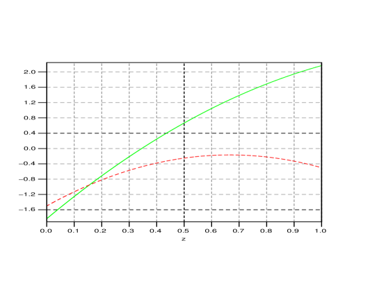
Figure 3: Anti-brane potential in the absence of other branes (from the bracket on the RHS of (64)), assuming $h^{1,1}(X)=1$. The solid, green curve corresponds to charges $(\beta^{(p)})=(3,-2,-1)$. In this case the anti-brane is attracted to the positively charged boundary at $z=0$. The red, dashed curve corresponds to charges $(\beta^{(p)})=(2,-3,1)$. The anti-brane is attracted to either one of the boundaries, depending on its position $z$.

5.2 Threshold Corrections to the Gauge Kinetic Functions

Another set of quantities relevant for moduli stabilization which arise at second order in $\kappa_{11}^{\frac{2}{3}}$ are the threshold corrections to the gauge kinetic functions. Again, we are fortunate. Standard arguments [51] tell us that these are among the few terms which can be reliably calculated at this order. The arguments are slightly altered in the current situation, but are essentially unchanged.

Consider the possible sources of second order contributions to the gauge kinetic functions. One possible source is higher order terms involving the gauge field strengths in the higher dimensional action. Clearly, such terms can only occur on the boundaries where the gauge fields are located. Dimensional analysis shows that such contributions are either all higher order or, possibly, come with a non-integer power of $\kappa_{11}^{2/3}$. This latter possibility is probably forbidden by the supersymmetry of the five-dimensional theory and, in any case, cannot mix with the terms we wish to calculate. Therefore, we will assume that such terms do not occur.

Another possible source of second order terms in the gauge kinetic functions are $\kappa_{11}^{\frac{4}{3}}$ terms in the warping. Clearly, substituting such a piece of the background into the boundary actions will give contributions that are higher order than we are interested in. Substituted into the bulk theory, such second order contributions to the warping will not contribute to the four-dimensional effective action if there is a zero mode associated with them. This is because the zero mode is defined to be the orbifold average and, hence, the linear perturbation of order $\kappa_{11}^{\frac{4}{3}}$ drops out upon performing the integration over the orbifold direction. This is not quite true for some of the background pieces in $G$ and ${\cal A}$. These could, in principle, contribute to the kind of terms we are interested in. However, in the supersymmetric case the results obtained were consistent with these contributions being zero. In other words, the complex structure determined from the moduli kinetic terms, and the requirement that the gauge kinetic functions be holomorphic, are consistent with there being no additional terms of this type. This is a highly non-trivial statement and is unlikely to have occurred by chance. We will assume that these terms are also absent in the non-supersymmetric case. This assumption leads us to a result which is consistent with all of the symmetries present in this situation, including being invariant under the transformations (57)–(60). This constitutes a highly non-trivial check of its veracity.

The crucial point, once one has concluded that the above contributions do not occur, is that all other ways of generating second order terms in the gauge kinetic functions are explicitly calculable using pieces of the action and the background solution that we know. One obvious contribution arises by inserting the domain wall solution into the boundary Yang-Mills actions. Other, more subtle, contributions arise from the additional warping of bulk fields caused by fluctuations on the boundary. For example, the four-dimensional metric receives a warping that is bilinear in the boundary gauge field strengths. This warping will lead to order an $\kappa_{11}^{\frac{4}{3}}$ correction to the gauge kinetic function via cross terms with the domain wall warping. The full expressions for the warpings of the bulk fields that are needed in the calculation are given in Appendix D. However, we find that all contributions due to warping induced by field fluctuations drop out, just as they did in the supersymmetric case [51]. This means that, in the end, the threshold corrections to the gauge kinetic functions are simply determined by the warping of the domain wall solution. Explicitly, to order $\kappa_{11}^{\frac{4}{3}}$, we find that the Yang-Mills part of the four-dimensional effective theory is given by

$$S_{4}^{\textnormal{GKF}} = \frac{-1}{32\pi\alpha_{\textnormal{GUT}}}\int d^{4}x\sqrt{-g_{4}}\left[\left(e^{\phi}+\epsilon_{0}e^{\beta}b^{k}\left(\sum_{p=0}^{N+1}\tau_{k}^{(p)}\left(z_{(p)}^{2}-2z_{(p)}\right)+\frac{4}{3}\delta_{k}\right)\right)\textnormal{tr}(F^{2}_{(0)})\right.$$ (67)

$$\left.\qquad\qquad\qquad\qquad\qquad+\left(e^{\phi}+\epsilon_{0}e^{\beta}b^{k}\left(\sum_{p=0}^{N+1}\tau^{(p)}_{k}z_{(p)}^{2}-\frac{2}{3}\delta_{k}\right)\right)\textnormal{tr}(F^{2}_{(N+1)})\right.$$

$$\left.-\frac{1}{2}\left(\sigma+2\epsilon_{0}\left(\sum_{p=1}^{N}\beta^{(p)}_{k}\chi^{k}\left(z_{(p)}^{2}-2z_{(p)}\right)-\beta^{(N+1)}_{k}\chi^{k}+2\sum_{p=1}^{N}\tau^{(p)}_{k}(n^{k}_{(p)}\nu_{(p)})\right)\right)\epsilon_{\mu\nu\rho\sigma}F_{(0)}^{\mu\nu}F_{(0)}^{\rho\sigma}\right.$$

$$\left.-\frac{1}{2}\left(\sigma+2\epsilon_{0}\left(\sum_{p=1}^{N}\beta^{(p)}_{k}\chi^{k}z_{(p)}^{2}+\beta_{k}^{(N+1)}\chi^{k}\right)\right)\epsilon_{\mu\nu\rho\sigma}F_{(N+1)}^{\mu\nu}F_{(N+1)}^{\rho\sigma}\right].$$

Despite the fact that our theory is not supersymmetric, we can express this result in terms of two ‘gauge kinetic functions’. One simply defines the real and imaginary parts of these objects to be given by the coefficients of the $\textnormal{tr}F^{2}$ and $\epsilon FF$ terms as usual. We find that

$$f_{(0)} = \left(e^{\phi}+\epsilon_{0}e^{\beta}b^{k}\left(\sum_{p=0}^{N+1}\tau_{k}^{(p)}\left(z_{(p)}^{2}-2z_{(p)}\right)+\frac{4}{3}\delta_{k}\right)\right)$$

$$+i\left(\sigma+2\epsilon_{0}\left(\sum_{p=1}^{N}\beta^{(p)}_{k}\chi^{k}\left(z_{(p)}^{2}-2z_{(p)}\right)-\beta^{(N+1)}_{k}\chi^{k}+2\sum_{p=1}^{N}\tau^{(p)}_{k}(n^{k}_{(p)}\nu_{(p)})\right)\right)$$

$$f_{(N+1)} = \left(e^{\phi}+\epsilon_{0}e^{\beta}b^{k}\left(\sum_{p=0}^{N+1}\tau^{(p)}_{k}z_{(p)}^{2}-\frac{2}{3}\delta_{k}\right)\right)+i\left(\sigma+2\epsilon_{0}\left(\sum_{p=1}^{N}\beta^{(p)}_{k}\chi^{k}z_{(p)}^{2}+\beta_{k}^{(N+1)}\chi^{k}\right)\right)$$ (69)

The explicit supersymmetry breaking in our theory means that these functions will no longer be holomorphic when expressed in terms of the superfields defined in (41)–(45). We will see this explicitly below.

Some comments about this result are in order.

• As was the case for the first order results, this expression is valid when we change an arbitrary number of our branes into anti-branes. In this case, the quantities $\delta_{k}$ should be taken to be the sum of the anti-brane tensions.

• The above result agrees with that of standard heterotic M-theory upon taking $\delta_{k}\rightarrow 0$. Despite the fact that these terms are second order in our expansion, they only contain a single power of the brane charges. This is necessarily the case, given that the gauge fields themselves only appear at order $\kappa_{11}^{\frac{2}{3}}$. This means that all of the threshold corrections to the gauge kinetic functions can be made small by tuning the $b^{k}$, $\chi^{k}$ and $\nu_{(p)}$ moduli appropriately. In fact, an inspection of (67) reveals that it suffices to set the volume $\delta_{k}b^{k}$ of the anti-brane cycle and the associated linear combination $\delta_{k}\chi^{k}$ of the $\chi^{k}$ axions to zero.

• We can write the result as a supersymmetric piece plus explicit supersymmetry breaking terms, using the definition of superfields in (41)–(45). This leads to a gauge kinetic function which is no longer holomorphic at second order in our expansions.

  $$f_{(0)} = S-\epsilon_{0}\left[\tau^{(N+1)}_{k}T^{k}+2\sum_{p=1}^{N}Z_{(p)}-\frac{2}{3}\delta_{k}(T^{k}+\bar{T}^{k})\right.$$

  $$\;\;\;\;\quad\quad\quad\quad\quad\left.+\delta_{k}(T^{k}-\bar{T}^{k})\left(\left(\frac{Z_{(\bar{p})}+\bar{Z}_{(\bar{p})}}{\bar{\tau}_{k}(T^{k}+\bar{T}^{k})}\right)^{2}-2\frac{Z_{(\bar{p})}+\bar{Z}_{(\bar{p})}}{\bar{\tau}_{k}(T^{k}+\bar{T}^{k})}\right)\right]$$

  $$f_{(N+1)} = S+\epsilon_{0}\left[\tau_{k}^{(N+1)}T^{k}-\frac{1}{3}\delta_{k}(T^{k}+\bar{T}^{k})-\delta_{k}(T^{k}-\bar{T}^{k})\left(\frac{Z_{(\bar{p})}+\bar{Z}_{(\bar{p})}}{\bar{\tau}_{k}(T^{k}+\bar{T}^{k})}\right)^{2}\right]$$ (71)

  The above result looks complicated, despite the fact that the component forms of the gauge kinetic functions, given in (5.2,69), are quite close to the usual result for heterotic M-theory. This is because, in many of the terms in the imaginary parts of these functions, it is the charge, and not the tension, of the extended objects which appears. The complex structure derived in subsection 4.2 contained the tensions rather than the charges. Therefore, we have to add contributions proportional to $\delta_{k}$ to the standard holomorphic quantity in order to correct this difference.

• At first glance there appears to be a strange asymmetry in the results (• ‣ 5.2) and (71) between the $(0)$ and $(N+1)$ fixed planes. For example, there is a linear term in $Z_{(p)}$ in (• ‣ 5.2) but not in (71). This asymmetry is an artifact of the fact that we measure the position of the branes as a distance from the $(0)$ plane and the complicated way in which the component scalar fields are combined in the ${\cal N}=1$ structure (41)-(45). In fact if we apply the transformations (61)-(63), corresponding to inverting the $y$ direction in Fig. 1, we find that the above gauge kinetic functions turn into one another as they should. This is a highly non-trivial test of our results.

  One could of course simply relabel the branes, swapping $(0)$ and $(N+1)$ if one so desired. Such a change of notation is useful in relating these results to some of the previous literature. We note in addition that either of the fixed planes can be the hidden sector. Which plays this role is determined by such factors as the choices of the tensions $\tau^{(p)}_{k}$.

• Note that these corrections to the gauge kinetic functions arise at order $\epsilon_{S}$, while the brane forces appear at order $\epsilon_{S}^{2}$. Hence, if we wish to include the effects of gaugino condensation, this modification of the gauge kinetic functions is likely to be relevant in regions of moduli space where the exponential suppression is not too strong. This appears to have been missed in the literature so far. This is not surprising, given the need for a full calculation of the back-reaction of the anti-brane before such corrections become evident.

  The importance of these terms has already been demonstrated in Fig. 2, where we have plotted the warping of the Calabi-Yau volume across the orbifold. The values of this warping at the boundaries, $z=0,1$, correspond precisely to the real parts of the two gauge kinetic functions above. What we have seen is that the introduction of an anti-brane can turn the weakly coupled boundary into the strongly coupled one and vice versa.

6 A Simple Example

The reader interested in analyzing the physics of anti-branes in four-dimensional heterotic M-theory may not wish to wade through the details of the dimensional reduction presented in the proceeding sections. With this in mind, we now provide a simple example extracted from our general analysis.

Let us consider the case where there is only a single Kähler modulus for the Calabi-Yau manifold, a single anti-brane and no branes in the bulk. Then action (35) and the second order action $S_{\delta^{1,2}}^{(2)}$ with potential (64) become

$$S=S_{\delta^{0}}^{(0,1)}+S_{\delta^{1}}^{(1)}+S_{\delta^{1,2}}^{(2)},$$ (72)

where

$$S_{\delta^{0}}^{(0,1)} = -\frac{1}{2\kappa_{4}^{2}}\int d^{4}x\sqrt{-g_{4}}\left[\frac{1}{2}R_{4}+\frac{3}{4}(\partial\beta)^{2}+\frac{1}{4}(\partial\phi)^{2}+\frac{1}{4}e^{-2\phi}(\partial\sigma)^{2}+3e^{-2\beta}(\partial\chi)^{2}\right.$$

$$+ \left.2\epsilon_{0}\bar{z}e^{-2\phi}\partial\sigma\partial\bar{\nu}+\frac{1}{2}\epsilon_{0}\bar{\tau}e^{\beta-\phi}(\partial\bar{z})^{2}+2\epsilon_{0}\bar{\tau}e^{-\phi-\beta}\left(\chi^{2}(\partial\bar{z})^{2}-2\frac{\chi}{\bar{\tau}}\partial\bar{\nu}\partial\bar{z}+\frac{1}{\bar{\tau}^{2}}(\partial\bar{\nu})^{2}\right)\right]$$

$$S_{\delta^{1}}^{(1)} = -\frac{1}{2\kappa_{4}^{2}}\int d^{4}x\sqrt{-g_{4}}\left[\frac{2\epsilon_{0}}{(\pi\rho)^{2}}\delta e^{-2\beta-\phi}\right]$$ (74)

and

$$S_{\delta^{1,2}}^{(2)}=-\frac{1}{2\kappa_{4}^{2}}\int d^{4}x\sqrt{-g_{4}}\left[\frac{2\epsilon_{0}^{2}}{3(\pi\rho)^{2}}e^{-\beta-2\phi}\delta\left((\tau_{(0)}-\tau_{(2)})\bar{z}+\bar{\tau}(1-\bar{z})\bar{z}+\tau_{(2)}-\frac{2}{3}\delta\right)\right].$$ (75)

Here we have only included the potential terms in $S^{(2)}_{\delta^{1,2}}$, as described earlier in the paper. This action is valid when $\epsilon_{0}e^{\beta-\phi}<1$, where $\epsilon_{0}=(\pi\rho)^{\frac{4}{3}}2\pi v^{-\frac{1}{3}}\left(\frac{\kappa_{4}}{4\pi}\right)^{\frac{2}{3}}$ for the conventions chosen here. The system consists of four-dimensional gravity and six scalar fields, $\phi$, $\beta$, and $\bar{z}$ as well as $\sigma$, $\chi$ and $\bar{\nu}$. The volume of the Calabi-Yau space in fundamental units is given by $ve^{\phi}$, the separation of the orbifold fixed planes in five dimensions by $\pi\rho e^{\beta}$ and, finally, $\bar{z}$ is the position modulus of the anti-brane. In these expressions $v$ and $\pi\rho$ are reference constants, which can be chosen arbitrarily. They define the physical meaning of the moduli $\phi$ and $\beta$. The remaining three scalars are the axions corresponding to these fields. The fields $\sigma$ and $\chi$ descend from bulk form fields in higher dimensions and $\bar{\nu}$ from a field living on the worldvolume of the anti-brane. A collision of the anti-brane with one of the two fixed planes occurs when the anti-brane modulus takes the value $\bar{z}=0$ or $\bar{z}=1$. The only quantities appearing in the action which remain to be explained are then $\bar{\tau}$, $\tau_{0}$ and $\tau_{2}$. These are integers which determine the tensions of the anti-brane and the orbifold fixed planes which the anti-brane collides with at $\bar{z}=0$ and $\bar{z}=1$ respectively. There are two restrictions on the choices which can be made for these parameters. First, $\bar{\tau}$ must be positive. Second, the three tensions must obey the condition $\tau_{0}-\bar{\tau}+\tau_{2}=0$.

Action (72) can also be expressed in terms of the ‘superfields’ defined in (41)-(45). For this simple example, these become

$$S = e^{\phi}+\epsilon_{0}\bar{\tau}e^{\beta}\bar{z}^{2}+i\left(\sigma+2\epsilon_{0}\bar{\tau}\chi\bar{z}^{2}\right)$$ (76)

$$T = e^{\beta}+2i\chi$$ (77)

$$Z = \bar{\tau}e^{\beta}\bar{z}+2i(\bar{\nu}+\chi\bar{\tau}\bar{z}).$$ (78)

First consider $S_{\delta^{0}}^{(0,1)}$ in (6). This part of the action is independent of the parameter $\delta$. Hence, it is supersymmetric and can be expressed in terms of a Kähler potential and a superpotential. Since this simplified theory only contains the dilaton and moduli, the superpotential vanishes. We find the Kähler potential to be

$$\kappa_{4}^{2}K=-3\log\left[T+\bar{T}\right]-\log\left[S+\bar{S}-\epsilon_{0}\frac{(Z+\bar{Z})^{2}}{\bar{\tau}(T+\bar{T})}\right]+\log 8.$$ (79)

In calculating the kinetic terms, the results obtained from this expression are valid to first order in $\epsilon_{0}e^{\beta-\phi}$.

Now consider $S_{\delta^{1}}^{(1)}$ and $S_{\delta^{1,2}}^{(2)}$. These terms are proportional to at least one power of $\delta$. Hence, they are explicitly associated with the non-supersymmetric part of the theory and we do not write them in terms of a Kähler potential and a superpotential. Be that as it may, they can be expressed in terms of the scalar fields in (76-78). Recognizing that (74) and (75) contribute potential energy terms ${\cal{V}}_{1}$ and ${\cal{V}}_{2}$ respectively, we find that the total potential induced by the anti five-brane is

$${\cal V}={\cal V}_{1}+{\cal V}_{2},$$ (80)

where

$${\cal V}_{1} = \kappa_{4}^{-2}\frac{\epsilon_{0}}{(\pi\rho)^{2}}\delta(T+\bar{T})e^{\kappa_{4}^{2}K}$$ (81)

$${\cal V}_{2} = \frac{1}{24}\kappa_{4}^{-2}\frac{\epsilon_{0}^{2}}{(\pi\rho)^{2}}\delta e^{2\kappa_{4}^{2}K}(T+\bar{T})^{5}\left[2\frac{\tau_{(0)}}{\bar{\tau}}\frac{Z+\bar{Z}}{T+\bar{T}}-\frac{1}{\bar{\tau}}\left(\frac{Z+\bar{Z}}{T+\bar{T}}\right)^{2}+\tau_{(2)}-\frac{2}{3}\delta\right].$$ (82)

This simple example includes the essentials of the features of the potential outlined in the main text. In particular, while the first term of (75) represents the Coulomb forces acting on the anti-brane, the second, third and fourth terms are the new contributions to the potential that we have discussed.

The gauge kinetic functions in this simple example are the following.

$$f_{(0)} = e^{\phi}+\epsilon_{0}e^{\beta}\left(\bar{\tau}(\bar{z}^{2}-2\bar{z})+\frac{4}{3}\delta\right)+i\left(\sigma+2\epsilon_{0}(-\bar{\tau}\chi(\bar{z}^{2}-2\bar{z})-\tau_{(2)}\chi+2\bar{\nu})\right)\;$$ (83)

$$f_{(2)} = e^{\phi}+\epsilon_{0}e^{\beta}\left(\bar{\tau}\bar{z}^{2}-\frac{2}{3}\delta\right)+i\left(\sigma+2\epsilon_{0}\left(-\bar{\tau}\chi\bar{z}^{2}+\tau_{(2)}\chi\right)\right).\;$$ (84)

These expressions correspond to the orbifold fixed planes at $\bar{z}=0$ and $\bar{z}=1$ respectively. The real parts of these functions reproduce the inverse square of the gauge couplings of the gauge fields living upon the fixed planes, while the imaginary parts reproduce the theta terms. Again, one can rewrite these results in terms of the field definitions (76)-(78). The result is

$$f_{(0)} = S-\epsilon_{0}\left[\tau_{(2)}T+2Z-\frac{2}{3}\delta(T+\bar{T})+\delta(T-\bar{T})\left(\left(\frac{Z+\bar{Z}}{\bar{\tau}(T+\bar{T})}\right)^{2}-2\frac{Z+\bar{Z}}{\bar{\tau}(T+\bar{T})}\right)\right]$$ (85)

$$f_{(2)} = S+\epsilon_{0}\left[\tau_{(2)}T-\frac{1}{3}\delta(T+\bar{T})-\delta(T-\bar{T})\left(\frac{Z+\bar{Z}}{\bar{\tau}(T+\bar{T})}\right)^{2}\right].$$ (86)

Note that the gauge kinetic functions are holomorphic in these complex fields in the formal limit that $\delta\rightarrow 0$. This is as it should be, since this corresponds to turning off the supersymmetry breaking induced by the anti-branes. The terms proportional to $\delta$ break supersymmetry and, accordingly, are not holomorphic in the fields (76)-(78). The fact that no single choice of complex fields is possible which simultaneously allows the kinetic terms in (6) to be reproduced from a Kähler potential and makes the functions (85) and (86) holomorphic demonstrates that the presence of the anti-brane breaks supersymmetry explicitly. The modifications to the gauge kinetic functions due to the presence of the anti-brane are crucial in any discussion of gaugino condensation. These corrections can even exchange the weakly and strongly coupled fixed planes, interchanging what would be naively thought of as the visible and hidden sectors. Note that, for suitable choices of the parameters described above, either fixed plane can be the hidden sector.

Action (72), together with the gauge kinetic functions (85) and (86), can be used as the starting point for analyzing the physics of anti-branes in perturbative heterotic M-theory.

7 Conclusions

In this paper, we derived the bosonic four-dimensional effective theory for heterotic M-theory in the presence of M five-branes and anti M five-branes. The starting point of our analysis is the five-dimensional action of heterotic M-theory, where the M five-branes appear as three-branes. We have explicitly computed the case with an arbitrary number of three-branes but only one anti three-brane. However, it is straightforward to generalize our results to an arbitrary number of anti three-branes.

We first found a suitable background solution to five-dimensional heterotic M-theory on which to reduce to four-dimensions. This solution is a non-supersymmetric domain wall, presented in Section 3, which is a generalization of the BPS domain wall background in the supersymmetric case, that is, in the absence of anti-branes. We found that this domain wall solution can be computed as an expansion in the strong coupling parameter $\epsilon_{S}$, and we presented the result up to first order in this parameter. A new feature induced by the anti-brane is warping quadratic in the orbifold coordinate. This occurs in addition to the linear warping which is characteristic of the BPS domain wall in the supersymmetric theory.

We then computed the four-dimensional bosonic effective action on this domain wall background as an expansion in $\kappa_{11}^{\frac{2}{3}}$. We stress that this calculation includes the back-reaction effects of the branes as well as the anti-branes. In particular, there is no assumption of a small anti-brane charge underlying our calculation. To zeroth and first order in this expansion, we found that the bosonic theory is given by the supersymmetric result plus the addition of a single potential term. This “uplifting potential” is generated by the anti-brane and has a number of interesting properties. First of all, at this order, it is independent of the brane position moduli and only depends on the dilaton and the Calabi-Yau Kähler moduli. More precisely, it is proportional to the volume of the cycle wrapped by the anti brane, as well as to the strong coupling parameter $\epsilon_{S}$. Since, necessarily, $\epsilon_{S}\ll 1$ (for four dimensional heterotic M-theory to be a good description of the system) the uplifting potential is suppressed.

We have also calculated a number of terms in the four-dimensional effective action at second order, that is, at order $\kappa_{11}^{\frac{4}{3}}$. We have specifically focused on terms where new qualitative features, not seen at lower order, occur. In particular, we explicitly calculated the second order contributions to the anti-brane potential. This gives interactions between branes and anti-branes. This potential is of order $\epsilon_{S}^{2}$ and, hence, even further suppressed relative to the leading uplifting potential. The $\epsilon_{S}$ suppression of the perturbative potential has important implications for moduli stabilization, since the stabilization mechanism involves an interplay between perturbative and non-perturbative effects. For stabilization to occur, both types of effects should be roughly comparable in size. This is greatly facilitated by the suppression of the perturbative potential. While the second order brane potential includes the expected “Coulomb-like” forces between the branes and the anti-brane, we find, in addition, an unexpected force between these objects which also arises from their back-reaction.

The other terms we have computed at second order are the corrections to the Yang-Mills gauge couplings and theta angles. We find that these threshold corrections depend on the brane as well as the anti-brane moduli and lead to a non-holomorphic “gauge kinetic function”. This dependence on the anti-brane modulus and the non-holomorphicity has important consequences for gaugino condensation. This will be the subject of a forthcoming paper [48].

We believe that some of the features found in this paper, for example the non-Coulomb type brane-brane forces due to anti-brane back-reaction and the non-holomorphic corrections to the gauge kinetic function, may arise in other models with anti-branes, for example, in the context of IIB string theory. To our knowledge, this has not yet been studied. Our results have important applications to moduli stabilization in heterotic models with anti-branes, supersymmetry breaking due to anti-branes and the cosmology of such models. In particular, given that the anti-brane can be attracted to the boundary by the perturbative forces while it is repelled due to membrane instanton effects, we have argued that stabilization of the anti-brane due to a combination of perturbative and non-perturbative effects can be achieved. These issues are currently under investigation [48].

Acknowledgments
A. L. is supported by the EC 6th Framework Programme MRTN-CT-2004-503369. J. G. is supported by CNRS and in part for this research by the National Science Foundation under Grant No. PHY99-07949. The work of B. A. O is supported in part by the DOE under contract No. DE-AC02-76-ER-03071 and by the NSF Focused Research Grant DMS0139799. J. G. and A. L. would like to thank the Department of Physics of the University of Pennsylvania, where part of this work was carried out, for generous hospitality.

Appendix: Origins of Quantities in the Five-Dimensional Theory.

In this appendix we explain the origin of the fields and quantities which appear in the action (2.1) of five-dimensional heterotic M-theory in terms of the underlying 11-dimensional theory [49], compactified on a Calabi-Yau manifold $X$. All of these results are standard and can be found in the literature [55, 36, 37], but are here included for completeness. The last part of the appendix presents a number of technical results for the five-dimensional warping which are needed for the calculation in the main part of the paper.

Appendix A Origin of the Five-Dimensional Bulk Theory

The bulk fields in the five-dimensional action (2.1) originate from zero modes of the 11-dimensional metric and three-form on the Calabi-Yau manifold $X$. Let us start by discussing the metric moduli.

In addition to the five-dimensional metric, the 11-dimensional metric gives rise to a number of scalar fields which parametrize the Calabi-Yau moduli space. As is well known, this space is (locally) a direct product of the Kähler moduli space, parametrized by the periods of the Kähler form $\omega$, and the complex structure moduli space, parametrized by periods of the holomorphic three-form $\Omega$. Let us first discuss the Kähler moduli space. We introduce an integral basis $C^{k}$, where $k,l,\dots=1,\dots,h^{1,1}(X)$, of the second homology of the Calabi-Yau manifold and a dual basis $v^{-1/3}\omega_{k}$ of harmonic $(1,1)$ forms satisfying

$$\frac{1}{v^{1/3}}\int_{C^{k}}\omega_{l}=\delta_{l}^{k}\;.$$ (87)

The $h^{1,1}(X)$ Kähler moduli $a^{k}$ can then be defined by expanding $\omega=a^{k}\omega_{k}$. The Kähler moduli space metric $G_{kl}(a)$ is then given by

$$G_{kl}(a)\equiv\frac{1}{vV}\int_{X}\omega_{k}\wedge\star\omega_{l}=\frac{\partial}{\partial a^{k}}\frac{\partial}{\partial a^{l}}K(a)$$ (88)

where the Kähler potential $K(a)$ is given by $K(a)=-\ln(d_{klm}a^{k}a^{l}a^{m})$ with the triple intersection numbers

$$d_{klm}=\frac{1}{v}\int_{X}\omega_{k}\wedge\omega_{l}\wedge\omega_{m}\;.$$ (89)

It is easy to show that the total Calabi-Yau volume V can be written as

$$V=\frac{1}{v}\int_{X}\sqrt{g}=\frac{1}{6}d_{ijk}a^{i}a^{j}a^{k}\;.$$ (90)

In the context of the five-dimensional theory it is more appropriate to work with the rescaled Kähler moduli $b^{k}=V^{-1/3}a^{k}$ which satisfy the constraint $e^{-K(b)}=d_{klm}b^{k}b^{l}b^{m}=6$. They constitute $h^{1,1}(X)-1$ independent fields which will be used in the five-dimensional action alongside $V$ as the remaining independent degree of freedom. Accordingly, the five-dimensional theory is formulated in terms of the metric $G_{kl}(b)=V^{2/3}G_{kl}(a)$ which we frequently denote by simply $G_{kl}$ in the text. It is useful to define lowered index fields $b_{k}=G_{kl}(b)b^{l}$. It follows directly from the explicit form of the metric that $b_{k}b^{k}=3$, which, upon treating the $b^{k}$ as five-dimensional fields, leads to the identities

$$b_{k}\partial_{\alpha}b^{k}=0\;,$$ (91)

$$b_{k}\left(\nabla_{\alpha}\nabla^{\alpha}b^{k}+\Gamma^{k}_{lm}(b)\partial_{\alpha}b^{l}\partial^{\alpha}b^{m}\right)=0\;.$$ (92)

Here, $\Gamma^{k}_{lm}(b)$ is the connection associated to the moduli space metric $G_{kl}(b)$ and and $\nabla_{\alpha}$ is the five-dimensional covariant derivative. These relations are useful in deriving the result for the domain wall warping of $b^{k}$, (30).

We now move on to the complex structure moduli space of the Calabi-Yau. To this end, we introduce a symplectic basis $(a^{A},b_{B})$, where $A,B,\dots=0,\dots,h^{2,1}(X)$ of the third homology and a dual basis $(\alpha_{A},\beta^{B})$ of harmonic three-forms satisfying the standard relations

$$\int_{X}\alpha_{B}\wedge\beta^{A}=\int_{a^{A}}\alpha_{B}=\delta_{B}^{A}\;,\quad\int_{X}\beta^{A}\wedge\alpha_{B}=\int_{b_{B}}\beta^{A}=-\delta_{B}^{A}$$ (93)

with all other integrals zero. The complex structure moduli space can be parametrized by the periods $({\cal Z}^{A},{\cal G}_{B})$ defined by

$${\cal Z}^{A}=\int_{a^{A}}\Omega\;,\quad{\cal G}_{B}=\int_{b_{B}}\Omega\,.$$ (94)

It turns out, that the periods ${\cal G}_{B}$ are, in fact, functions of the ${\cal Z}^{A}$ and can be obtained as derivatives ${\cal G}_{B}=\frac{\partial}{{\cal Z}^{B}}{\cal G}$ of a holomorphic pre-potential ${\cal G}$. The complex structure moduli Kähler potential is then given by

$${\cal K}({\cal Z})=-\mbox{ln}\left(i\int_{X}\Omega\wedge\bar{\Omega}\right)=-\mbox{ln}\left({\cal G}_{B}\bar{{\cal Z}}^{B}-\bar{{\cal G}}_{B}{\cal Z}^{B}\right)\;.$$ (95)

The ${\cal Z}^{A}$ are homogeneous coordinates and the physical degrees of freedom are identified with the affine coordinates ${\mathfrak{z}}^{a}={\cal Z}^{a}/{\cal Z}^{0}$, where $a,b,\dots=1,\dots,h^{2,1}(X)$. In terms of these physical fields the Kähler potential can be written as

$${\cal K}({\mathfrak{z}})=-\mbox{ln}\left[2i({\cal G}-\bar{{\cal G}})-i({\mathfrak{z}}^{a}-\bar{{\mathfrak{z}}}^{a})\left(\frac{\partial{\cal G}}{\partial{\mathfrak{z}}^{a}}+\frac{\partial\bar{{\cal G}}}{\partial\bar{{\mathfrak{z}}}^{a}}\right)\right]\;,$$ (96)

and the associated metric is obtained in the usual way as ${\cal K}_{p\bar{q}}({\mathfrak{z}})=\frac{\partial}{\partial p}\frac{\partial}{\partial\bar{q}}{\cal K}({\mathfrak{z}})$. The final quantity we need to know about is the matrix $M$ which appears in some of the five dimensional kinetic terms. It is defined as follows.

$$M_{AB}=\bar{{\cal G}}_{AB}+T_{AB}\,,\qquad T_{AB}=2i\frac{\mbox{Im}{\cal G}_{AC}{\cal Z}^{C}\;\mbox{Im}{\cal G}_{BD}{\cal Z}^{D}}{{\cal Z}^{E}\mbox{Im}{\cal G}_{EF}{\cal Z}^{F}}\;,$$ (97)

where ${\cal G}_{AB}$ is the second derivative of the pre-potential ${\cal G}$.

Finally, we need to discuss the five-dimensional bulk fields which originate from the 11-dimensional three-form. The purely external part of this three-form gives rise to a three-form $C_{\alpha\beta\gamma}$ in the five-dimensional theory (which can be dualized to a scalar). The internal part, on the other hand, can be expanded in terms of our symplectic basis $(a^{A},b_{B})$ and, hence, gives rise to $2(h^{2,1}(X)+1)$ real scalar fields $\xi^{B}$ and $\tilde{\xi}_{A}$. This completes our discussion of the 11-dimensional origin of the bulk theory in five dimensions. It is explained in Section 2.1 how these fields are arranged into five-dimensional super-multiplets.

Appendix B Origin of the Five-Dimensional Boundary Theories

The matter field structure seen in the five dimensional theory comes from an appropriate dimensional reduction of the ten dimensional $E_{8}$ super-Yang-Mills theories residing on each of the two orbifold fixed planes. Given that we will introduce an arbitrary number, $N$, of M five-branes in our compactifications, we will label the two boundaries by $p=0,N+1$. On both orbifold planes we have stable holomorphic gauge bundles $V_{p}$ with structure groups $G_{(p)}$ residing on the Calabi-Yau manifold $X$. The commutants $H_{(p)}$ of $G_{(p)}$ within $E_{8}$ are the low-energy gauge groups which appear on the four-dimensional boundaries of five-dimensional heterotic M-theory. In order to discuss matter fields we need to decompose the adjoint representation of $E_{8}$, ${\bf 248}_{E_{8}}$, under $G_{(p)}\times H_{(p)}$. We write

$${\bf 248}_{E_{8}}=\sum(S_{(p)},R_{(p)})\;,$$ (98)

where $S_{(p)}$ and $R_{(p)}$ denote representations of $G_{(p)}$ and $H_{(p)}$, respectively. On the four-dimensional boundaries we have, in addition to gauge fields with gauge group $H_{(p)}$, matter fields transforming in the representations $R_{(p)}$ which appear in the decomposition (98). Their number is given by $h^{1}(X,V_{R_{(p)}})$, where $V_{R_{(p)}}$ is the associated bundle in the representation $R_{(p)}$. We will denote these matter fields by $C_{(p)}^{Ix}$ where indices $I,J,\dots$ run over all irreducible $R_{(p)}$ representations and indices $x,y,\dots$ label states within each representation. Further, we denote by $u_{I}^{x}$ a basis of one-forms for the cohomology groups $H^{1}(X,V_{R_{(p)}})$. The matter field Kähler metric on the four-dimensional boundaries can then be formally defined as

$$G_{(p)IJ}=\frac{1}{vV^{2/3}}\int_{X}u_{I}^{x}\wedge\star\bar{u}_{Jx}\;.$$ (99)

The connection $\Gamma_{(p)IJ}^{k}$ which appears in the five-dimensional Bianchi identities can then be written as

$$\Gamma^{k}_{(p)IJ}=G^{kl}(b)\frac{\partial}{\partial b^{l}}G_{(p)IJ}\;.$$ (100)

For the Yukawa couplings we can write

$$\lambda_{IJK}=\frac{1}{\|\Omega\|^{2}}\int_{X}\Omega\wedge u_{I}^{x}\wedge u_{J}^{y}\wedge u_{K}^{z}f_{xyz}^{(IJK)}\;,$$ (101)

where $f_{xyz}^{(IJK)}$ projects onto the singlet of the internal gauge group $G_{(p)}$. The superpotentials $W_{(p)}$ are then given by

$$W_{(p)}=\sqrt{4\pi\alpha_{\rm GUT}}\sum_{I,J,K}\lambda_{IJK}f_{xyz}^{(IJK)}C_{(p)}^{Ix}C_{(p)}^{Jy}C_{(p)}^{Kz}\;.$$ (102)

Appendix C Origin of Three-Brane World-Volume Theories

As explained in the main part of the paper, we are interested in vacua with $N$ M five-branes, of which $N-1$ are ordinary five-branes and the remaining one is an anti five-brane. We label these branes by indices $p,q,\dots=1,\dots,N$ with $p=\bar{p}$ corresponding to the anti five-brane, as indicated in Fig. 1. The five-branes, $p\neq\bar{p}$, are wrapped on holomorphic curves with effective homology classes $C^{(p)}=\beta_{k}^{(p)}C^{k}$ within the Calabi-Yau manifold $X$, where $(C^{k})$ is the integral basis of the second homology of $X$ introduced earlier. The anti five-brane can be viewed as a five-brane wrapping a holomorphic curve with the “wrong” orientation and, hence, its class $C^{(\bar{p})}=\beta_{k}^{(\bar{p})}C^{k}$ corresponds to an anti-effective class (that is, $-C^{(\bar{p})}$ is effective).

In five-dimensional heterotic M-theory these five-branes appear as three-branes and we should discuss the fields on their world-volumes. From the 11-dimensional embedding coordinates of the five-branes we first have the position moduli $y_{(p)}$ in the orbifold direction and, possibly, additional scalar fields which describe the moduli space of the curves $C^{(p)}\subset X$. In this paper, we will not consider the latter fields explicitly. The purely internal part of the two-form on the five-brane world-volume (both indices in the direction of the curves) give rise to axions $s_{(p)}$ on the three-branes. Further let us introduce a standard basis $(a_{(p)u},b_{(p)w})$ of A and B cycles, where $u,w,\dots=1,\dots,g_{(p)}$ and $g_{(p)}$ is the genus of the $p^{\rm th}$ curve. In addition, we introduce a basis of holomorphic one-forms $(\alpha_{(p)u})$ on each curve, satisfying

$$\int_{a_{(p)u}}\alpha_{(p)w}=\delta_{uw}\;.$$ (103)

We can then expand the five-brane two form in this basis of one-forms which gives rise to $2g_{(p)}$ Abelian vector fields on the three-brane world-volumes. However, due to the self-duality of the five-brane two-form only half of these vector fields are independent and we will denote their field strengths by $E^{u}_{(p)\mu\nu}$. The period matrices

$$\Pi_{(p)uw}\equiv\int_{b_{(p)u}}\alpha_{(p)w}$$ (104)

then determine the gauge kinetic functions of these vector fields.

Appendix D Solution of the Bianchi Identities

In this appendix we collect the results for the warping of the five-dimensional bulk fields due to field fluctuations on the boundaries. These equations, which correspond to the 11-dimensional warping results obtained in Ref. [51], are needed for the reduction from five to four dimensions in the main part of the paper.

We start by solving the Bianchi identities (8)–(10). The Bianchi identity for the ${\cal F}^{k}$’s, (9), can be solved yielding the following result.

$${\cal F}^{k}_{\mu\nu} = (-2\kappa^{2}_{5})J^{(0)k}_{2\mu\nu}+2\kappa^{2}_{5}z(J^{(0)k}_{2\mu\nu}+J^{(N+1)k}_{2\mu\nu})$$ (105)

$${\cal F}^{k}_{\mu y} = \frac{-2\kappa^{2}_{5}}{\pi\rho}(\omega^{(0)k}_{1\nu}+\omega^{(N+1)k}_{1\nu})+\tilde{{\cal F}}^{k}_{\mu y}$$ (106)

The tilded quantity, $\tilde{{\cal F}}$, is an unspecified piece with trivial Bianchi identity, $d\tilde{{\cal F}}=0$, which can be fixed upon an examination of the equations of motion. We have also introduced the Chern-Simons one forms $\omega^{(p)k}$ which are defined by the relation $d\omega^{(p)k}_{1}=J^{(p)k}_{2}$, where $J^{(p)k}_{2}$ was defined in (12). Part of $\tilde{{\cal F}}$ is that due to the zero mode $\chi^{k}={\cal A}^{k}_{y}$. We also note that ${\cal A}_{\mu}$, being odd under the ${\mathbb{Z}}_{2}$ orbifold action, does not lead to zero modes. It turns out that the rest of the warping of ${\cal F}$ is not necessary for our present purposes. It drops out from the calculation of the four dimensional effective action.

The next set of terms from the five dimensional action that we need to dimensionally reduce are those involving the four-form field strength $G$. The solution to its Bianchi identity (8) is given by

$$G_{\mu\nu\rho\gamma} = -2\kappa^{2}_{5}J^{(0)}_{4\mu\nu\rho\gamma}+2\kappa^{2}_{5}z(J^{(0)}_{4\mu\nu\rho\gamma}+J^{(N+1)}_{4\mu\nu\rho\gamma})+\tilde{G}_{\mu\nu\rho\gamma}$$ (107)

$$G_{\nu\rho\gamma y} = \frac{-2\kappa^{2}_{5}}{\pi\rho}\frac{1}{16\pi\alpha_{\textnormal{ GUT}}}(\omega^{(0)}_{3\nu\rho\gamma}+\omega^{(N+2)}_{3\nu\rho\gamma})+\tilde{G}_{\nu\rho\gamma y}$$ (108)

Here $\tilde{G}$ is an unspecified contribution to the four form field strength which must be fixed upon an examination of the equations of motion. It obeys the trivial Bianchi Identity: $d\tilde{G}=0$. The quantities $\omega_{3}^{(p)}$ in (107) are Chern-Simons three-forms defined by the relations $d\omega^{(p)}_{3}=F_{(p)}\wedge F_{(p)}$. As a check of the integrability of this result we can find the associated three form potential contributions.

$$C_{\mu\nu\rho}=\frac{-2\kappa^{2}_{5}}{16\pi\alpha_{\textnormal{GUT}}}(\omega^{(0)}_{3\mu\nu\rho}-z(\omega^{(0)}_{3\mu\nu\rho}+\omega^{(N+1)}_{3\mu\nu\rho}))$$ (109)

The zero mode $B_{\mu\nu}=C_{y\mu\nu}$ with field strength $H_{\mu\nu\rho}$ is contained in the $\tilde{G}$ part of the above solution, along with other contributions to the warping which are irrelevant for our calculation.

Finally, we need to consider the Bianchi identity (10) for ${\cal X}^{A}$ and $\tilde{\cal X}_{B}$. In the absence of flux the solution to these Bianchi identities only give rise to higher order terms in the four-dimensional effective theory and are not explicitly needed.

For our calculation of the gauge kinetic functions to second order in subsection (5.2) we need explicit expressions for the warping of the metric and the Calabi-Yau volume modulus $V$ caused by field fluctuations on the boundaries. These warpings from fluctuations have to be added to the domain wall solution in section 3 to obtain the full expressions needed in the calculation.

$$\delta g_{\mu\nu} = \frac{\rho\kappa_{5}^{2}}{2\alpha_{\rm GUT}}\frac{b_{0}V_{0}}{a_{0}^{2}}\left[\left(\frac{1}{2}z^{2}-z+\frac{1}{3}\right){\rm tr}(F_{(0)\mu\gamma}{F_{(0)\nu}}^{\gamma})+\frac{1}{2}\left(z^{2}-\frac{1}{3}\right){\rm tr}(F_{(N+1)\mu\gamma}{F_{(N+1)\nu}}^{\gamma})\right]$$ (110)

$$\delta a = -\frac{\rho\kappa_{5}^{2}}{16\alpha_{\rm GUT}}\frac{b_{0}V_{0}}{a_{0}^{3}}\left[\left(\frac{1}{2}z^{2}-z+\frac{1}{3}\right){\rm tr}(F_{(0)}^{2})+\frac{1}{2}\left(z^{2}-\frac{1}{3}\right){\rm tr}(F_{(N+1)}^{2})\right]$$ (111)

$$\delta V = \frac{2V_{0}}{a_{0}}\delta a$$ (112)

References

- [1] S. Kachru, R. Kallosh, A. Linde and S. P. Trivedi, “De Sitter vacua in string theory,” Phys. Rev. D 68 (2003) 046005 [arXiv:hep-th/0301240].
- [2] M. Grana, “Flux compactifications in string theory: A comprehensive review,” Phys. Rept. 423 (2006) 91 [arXiv:hep-th/0509003].
- [3] J. P. Conlon, F. Quevedo and K. Suruliz, “Large-volume flux compactifications: Moduli spectrum and D3/D7 soft supersymmetry breaking,” JHEP 0508 (2005) 007 [arXiv:hep-th/0505076].
- [4] K. Choi, A. Falkowski, H. P. Nilles and M. Olechowski, “Soft supersymmetry breaking in KKLT flux compactification,” Nucl. Phys. B 718 (2005) 113 [arXiv:hep-th/0503216].
- [5] F. Denef, M. R. Douglas, B. Florea, A. Grassi and S. Kachru, “Fixing all moduli in a simple F-theory compactification,” arXiv:hep-th/0503124.
- [6] V. Balasubramanian, P. Berglund, J. P. Conlon and F. Quevedo, “Systematics of moduli stabilisation in Calabi-Yau flux compactifications,” JHEP 0503 (2005) 007 [arXiv:hep-th/0502058].
- [7] C. P. Burgess, P. G. Camara, S. P. de Alwis, S. B. Giddings, A. Maharana, F. Quevedo and K. Suruliz, “Warped supersymmetry breaking,” arXiv:hep-th/0610255.
- [8] A. Lukas, B. A. Ovrut and D. Waldram, “Non-standard embedding and five-branes in heterotic M-theory”, Phys.Rev. D59 (1999) 106005 [arXiv:hep-th/9808101]
- [9] R, Donagi, A. Lukas, B. A. Ovrut and D. Waldram, “Non-Perturbative Vacua and Particle Physics in M-Theory”, JHEP 9905 (1999) 018 [arXiv:hep-th/9811168]
- [10] R, Donagi, A. Lukas, B. A. Ovrut and D. Waldram, “Holomorphic vector bundles and non-perturbative vacua in M-theory ”, JHEP 9906 (1999) 034 [arXiv:hep-th/9901009]
- [11] R. Donagi, B. A. Ovrut, T. Pantev, D. Waldram, “Standard Model Bundles on Simply Connected Calabi-Yau Threefolds” JHEP 0108 (2001) 053 [arXiv:hep-th/0008008]
- [12] R. Friedman, J. W. Morgan and E. Witten, “Vector bundles and F-theory”, Comm. Math. Phys. 187(1997) 679 [arXiv:hep-th/9701162]
- [13] R, Donagi, “Principal bundles on elliptic fibrations”, Asian J. Math. 1(1997) 214 [arXiv:alg-geom/9702002]
- [14] R, Donagi, B. A. Ovrut, T. Pantev, D. Waldram, “Standard Model Bundles”, Adv.Theor.Math.Phys.5 (2002) 563-615 [arXiv:math-ag/0008010]
- [15] R, Donagi, B. A. Ovrut, T. Pantev, D. Waldram, “Spectral Involutions on Rational Elliptic Surfaces”, Adv.Theor.Math.Phys.5 (2002) 499-561 [arXiv:math-ag/0008011]
- [16] R. Donagi, Y. H. He, B. A. Ovrut and R. Reinbacher, “The spectra of heterotic standard model vacua,” JHEP 0506 (2005) 070 [arXiv:hep-th/0411156].
- [17] V. Braun, Y. H. He, B. A. Ovrut and T. Pantev, “A heterotic standard model,” Phys. Lett. B 618 (2005) 252 [arXiv:hep-th/0501070].
- [18] V. Braun, Y. H. He, B. A. Ovrut and T. Pantev, “A standard model from the E(8) x E(8) heterotic superstring,” JHEP 0506 (2005) 039 [arXiv:hep-th/0502155].
- [19] V. Braun, Y. H. He, B. A. Ovrut and T. Pantev, “Vector bundle extensions, sheaf cohomology, and the heterotic standard model,” arXiv:hep-th/0505041.
- [20] V. Braun, Y. H. He, B. A. Ovrut, and T. Pantev, “The exact MSSM spectrum from string theory,” JHEP 0605 (2006) 019 [arXiv:hep-th/0512177].
- [21] V. Braun, Y. H. He and B. A. Ovrut, “Stability of the minimal heterotic standard model bundle,” JHEP 0606 (2006) 032 [arXiv:hep-th/0602073].
- [22] V. Braun, Y. H. He, B. A. Ovrut, and T. Pantev, “Moduli dependent mu-terms in a heterotic standard model,” JHEP 0603 (2006) 006 [arXiv:hep-th/0510142].
- [23] V. Braun, Y. H. He, B. A. Ovrut, and T. Pantev, “Yukawa couplings in heterotic standard models,” JHEP 0604 (2006) 019 [arXiv:hep-th/0601204].
- [24] V. Braun, Y. H. He, B. A. Ovrut, and T. Pantev, “Heterotic standard model moduli,” JHEP 0601 (2006) 025 [arXiv:hep-th/0509051].
- [25] B. Andreas and G. Curio, “Standard models from heterotic string theory,” arXiv:hep-th/0602247.
- [26] A. E. Faraggi, E. Manno and C. Timirgaziu, “Minimal standard heterotic string models,” arXiv:hep-th/0610118.
- [27] O. Lebedev, H. P. Nilles, S. Raby, S. Ramos-Sanchez, M. Ratz, P. K. S. Vaudrevange and A. Wingerter, “A mini-landscape of exact MSSM spectra in heterotic orbifolds,” arXiv:hep-th/0611095. HEP-TH 0611095;
- [28] R. Blumenhagen, S. Moster, R. Reinbacher and T. Weigand, “Massless spectra of three generation U(N) heterotic string vacua,” arXiv:hep-th/0612039.
- [29] G. Lopes Cardoso, G. Curio, G. Dall’Agata, D. Lust, P. Manousselis and G. Zoupanos, “Non-Kaehler string backgrounds and their five torsion classes,” Nucl. Phys. B 652 (2003) 5 [arXiv:hep-th/0211118].
- [30] E. I. Buchbinder and B. A. Ovrut, “Vacuum stability in heterotic M-theory,” Phys. Rev. D 69 (2004) 086010 [arXiv:hep-th/0310112].
- [31] M. Becker, G. Curio and A. Krause, “De Sitter vacua from heterotic M-theory,” Nucl. Phys. B 693 (2004) 223 [arXiv:hep-th/0403027].
- [32] S. Gurrieri, A. Lukas and A. Micu, “Heterotic on half-flat,” Phys. Rev. D 70 (2004) 126009 [arXiv:hep-th/0408121].
- [33] G. Curio, A. Krause and D. Lust, “Moduli stabilization in the heterotic / IIB discretuum,” Fortsch. Phys. 54 (2006) 225 [arXiv:hep-th/0502168].
- [34] B. de Carlos, S. Gurrieri, A. Lukas and A. Micu, “Moduli stabilisation in heterotic string compactifications,” JHEP 0603 (2006) 005 [arXiv:hep-th/0507173].
- [35] V. Braun and B. A. Ovrut, “Stabilizing moduli with a positive cosmological constant in heterotic M-theory,” JHEP 0607 (2006) 035 [arXiv:hep-th/0603088].
- [36] A. Lukas, B. A. Ovrut, K. S. Stelle and D. Waldram, “The universe as a domain wall,” Phys. Rev. D 59 (1999) 086001 [arXiv:hep-th/9803235].
- [37] A. Lukas, B. A. Ovrut, K. S. Stelle and D. Waldram, “Heterotic M-theory in five dimensions,” Nucl. Phys. B 552 (1999) 246 [arXiv:hep-th/9806051].
- [38] M. Brandle and A. Lukas, “Five-branes in heterotic brane-world theories,” Phys. Rev. D 65, 064024 (2002) [arXiv:hep-th/0109173].
- [39] J. Khoury, B. A. Ovrut, P. J. Steinhardt and N. Turok, “The ekpyrotic universe: Colliding branes and the origin of the hot big bang,” Phys. Rev. D 64, 123522 (2001) [arXiv:hep-th/0103239].
- [40] E. J. Copeland, J. Gray and A. Lukas, “Moving five-branes in low-energy heterotic M-theory,” Phys. Rev. D 64 (2001) 126003 [arXiv:hep-th/0106285].
- [41] M. Bastero-Gil, E. J. Copeland, J. Gray, A. Lukas and M. Plumacher, “Baryogenesis by brane-collision,” Phys. Rev. D 66 (2002) 066005 [arXiv:hep-th/0201040].
- [42] E. J. Copeland, J. Gray, A. Lukas and D. Skinner, “Five-dimensional moving brane solutions with four-dimensional limiting behaviour,” Phys. Rev. D 66 (2002) 124007 [arXiv:hep-th/0207281].
- [43] B. de Carlos, J. Roberts and Y. Schmohe, “Moving five-branes and membrane instantons in low energy heterotic M-theory,” Phys. Rev. D 71 (2005) 026004 [arXiv:hep-th/0406171].
- [44] K. Becker, M. Becker and A. Krause, “M-theory inflation from multi M5-brane dynamics,” Nucl. Phys. B 715 (2005) 349 [arXiv:hep-th/0501130].
- [45] E. J. Copeland, J. Ellison, J. Roberts and A. Lukas, “Cosmological solutions of low-energy heterotic M-theory,” Phys. Rev. D 73 (2006) 086009 [arXiv:hep-th/0601173].
- [46] J. L. Lehners, P. McFadden and N. Turok, “Colliding branes in heterotic M-theory,” arXiv:hep-th/0611259.
- [47] J. L. Lehners, P. McFadden and N. Turok, “Effective actions for heterotic M-theory,” arXiv:hep-th/0612026.
- [48] J. Gray, A. Lukas and B. A. Ovrut, in preparation.
- [49] P. Horava and E. Witten, “Eleven-Dimensional Supergravity on a Manifold with Boundary,” Nucl. Phys. B 475 (1996) 94 [arXiv:hep-th/9603142].
- [50] E. Witten, “Strong Coupling Expansion Of Calabi-Yau Compactification,” Nucl. Phys. B 471, 135 (1996) [arXiv:hep-th/9602070].
- [51] A. Lukas, B. A. Ovrut and D. Waldram, “On the four-dimensional effective action of strongly coupled heterotic string theory,” Nucl. Phys. B 532, 43 (1998) [arXiv:hep-th/9710208].
- [52] A. Lukas, B. A. Ovrut and D. Waldram, “The ten-dimensional effective action of strongly coupled heterotic string theory,” Nucl. Phys. B 540, 230 (1999) [arXiv:hep-th/9801087].
- [53] A. Lukas, B. A. Ovrut and D. Waldram, “Non-standard embedding and five-branes in heterotic M-theory,” Phys. Rev. D 59, 106005 (1999) [arXiv:hep-th/9808101].
- [54] J. P. Derendinger and R. Sauser, “A five-brane modulus in the effective N = 1 supergravity of M-theory,” Nucl. Phys. B 598 (2001) 87 [arXiv:hep-th/0009054].
- [55] P. Candelas and X. de la Ossa, “Moduli space of Calabi-Yau manifolds,” Nucl. Phys. B 355, 455 (1991).