hep-th/0701022

CPHT-RR114.1206

Instabilities of Black Strings and Branes

Troels Harmark^a, Vasilis Niarchos^b and Niels A. Obers^a

^aThe Niels Bohr Institute

Blegdamsvej 17, 2100 Copenhagen Ø, Denmark

^b Centre de Physique Théorique

Ecole Polytechnique

91128 Palaiseau, France

harmark@nbi.dk, niarchos@cpht.polytechnique.fr, obers@nbi.dk

Abstract

We review recent progress on the instabilities of black strings and branes both for pure Einstein gravity as well as supergravity theories which are relevant for string theory. We focus mainly on Gregory-Laflamme instabilities. In the first part of the review we provide a detailed discussion of the classical gravitational instability of the neutral uniform black string in higher dimensional gravity. The uniform black string is part of a larger phase diagram of Kaluza-Klein black holes which will be discussed thoroughly. This phase diagram exhibits many interesting features including new phases, non-uniqueness and horizon-topology changing transitions. In the second part, we turn to charged black branes in supergravity and show how the Gregory-Laflamme instability of the neutral black string implies via a boost/U-duality map similar instabilities for non- and near-extremal smeared branes in string theory. We also comment on instabilities of D-brane bound states. The connection between classical and thermodynamic stability, known as the correlated stability conjecture, is also reviewed and illustrated with examples. Finally, we examine the holographic implications of the Gregory-Laflamme instability for a number of non-gravitational theories including Yang-Mills theories and Little String Theory.

Invited review for Classical and Quantum Gravity

1 Introduction

Gravitational instabilities were already considered around a hundred years ago by Sir James Jeans [1] in the context of Newtonian gravity, where it was shown that a static homogeneous non-relativistic fluid is unstable against long wavelength gravitational perturbations. Subsequently, with the advent of Einstein’s theory of general relativity, the perturbative stability of gravitational backgrounds such as black holes became an important issue. More recently, string theory has provided a plethora of higher dimensional black brane solutions which are captured at low energies by higher-dimensional (super)gravity theories. The question of perturbative stability in these backgrounds was examined by Gregory and Laflamme in 1993 in the seminal work [2, 3], where it was shown that neutral black strings in more than four dimensions suffer from a long wavelength instability, in close analogy to the Jeans instability. The main focus of this review will be the important progress that has been achieved over the last few years in understanding various aspects of the Gregory-Laflamme (GL) instability.

The classical stability of black holes is related closely to the central question of uniqueness in gravity. Black holes in four dimensions are known to be classically stable [4, 5]. This fits nicely with the fact that in four-dimensional vacuum gravity, a black hole in an asymptotically flat space-time is uniquely specified by the ADM mass and angular momentum measured at infinity [6, 7, 8, 9]. Uniqueness theorems [10, 11] for $D$-dimensional ($D>4$) asymptotically flat space-times state that the Schwarzschild-Tangherlini black hole solution [12] is the only static black hole in pure gravity. However, in pure gravity there are no uniqueness theorems for non-static black holes with $D>4$, or for black holes in space-times with non-flat asymptotics. On the contrary, there are known cases of non-uniqueness. An explicit example occurs in five dimensions for stationary solutions in asymptotically flat space-time: for a certain range of mass and angular momentum there exist both a rotating black hole with $S^{3}$ horizon [14] and rotating black rings with $S^{2}\times S^{1}$ horizons [15].

One may speculate [16] that a universally valid version of black hole uniqueness concerns only those solutions that are perturbatively stable. If this is true, then taking into account classical instability could restore the lost black hole uniqueness in higher dimensions. At present, there is no more than circumstantial evidence for this conjecture.

Beyond the question of uniqueness, instabilities in gravity are important because they are related to time-dependent phenomena and provide a glimpse into the full dynamics of the theory. Understanding the full time evolution of a condensing instability of a static or stationary solution and its end-point is an interesting and important problem that provides information about the full non-perturbative structure of the classical equations of motion. In this respect, information about the full structure of the static or stationary phases of the theory can provide important clues about the time-dependent trajectories that interpolate between different phases. In this review, we will see that black holes in spaces with compact directions exhibit a rich phase structure and give strong clues about time-dependent processes that involve exciting new dynamics like horizon topology changing transitions. In particular, for the Gregory-Laflamme instability of the neutral black string, a lot of the current research is inspired by the question [17, 18] of whether the Cosmic Censorship Hypothesis is violated [2, 3] in the condensation process of the Gregory-Laflamme instability, a process in which the topology of the horizon is conjectured to change.

While the stability properties of black holes in (super)gravity are interesting in their own right, their study is also highly relevant for the stability of black holes and branes in string theory. At low-energies closed string dynamics is captured by appropriate supergravity theories admitting a large variety of interesting solutions with event horizons that have received a lot of attention in the past decades. A particularly interesting class of solutions in string theory are the D-brane backgrounds. It has been conjectured [19, 20, 21, 22] that the near-horizon limit of these backgrounds is holographically dual to a non-gravitational theory living on the brane (or configuration of branes). This gauge/gravity (or AdS/CFT) correspondence implies a deep connection between the thermodynamics of the near-horizon brane backgrounds and the thermodynamics of the dual non-gravitational theories. For example, it suggests that the gauge theory dual of a classically unstable brane background must have a corresponding phase transition. This hints at an interesting connection between the classical stability of brane backgrounds and the thermodynamic stability of the dual non-gravitational theories.

In this review, we will discuss instabilities of black holes and branes in pure gravity and string theory. We will focus mainly on Gregory-Laflamme-type instabilities of black strings and branes that wrap or are smeared on a compact or non-compact direction, but along the way we will also comment on a variety of other related cases. The first part of this review (Sections 2-4) is a discussion that involves exclusively pure Einstein gravity in higher dimensions, and can be seen as separate from the second part which is more related to string theory. In this connection, we also refer the reader to the excellent review by Kol [27], which contains discussions on several important topics that we only briefly mention. In the second part (Sections 5-7), we turn to manifestations of the Gregory-Laflamme instability in supergravity solutions that are relevant for string theory and examine the implications for the holographically dual gauge theories and little string theory.

In the pure gravity case, we begin the discussion with an introduction to the Gregory-Laflamme instability of the neutral black string and its various manifestations. The black string metric is a solution of Einstein gravity in five or more dimensions that has a factorized form consisting of a Schwarzschild-Tangherlini black hole and an extra flat direction. It has been shown [2, 3] that this background suffers from a long wavelength instability, known as the Gregory-Laflamme instability, that involves perturbations with an oscillating profile along the direction of the string. We review the precise form of this perturbation including the (time-independent) threshold mode where the instability sets in. New features appear when the string direction is compactified. In this case, we find that the neutral black string has a critical mass, the Gregory-Laflamme mass, below which the solution is unstable.

The existence of the threshold mode at the critical mass strongly suggests that a new static non-uniform black string emerges at that point [28, 29]. In recent years, non-trivial information about the non-uniform black string solution [29, 30, 31, 32, 33] has been obtained with advanced numerical methods. One remarkable phenomenon of the non-uniform string is that it exhibits a critical dimension [31] (see also [34]) at which the phase transition of the uniform black string into the non-uniform black string changes from first order into second order. See also Refs. [31, 35, 36] for the large dimension behavior of the threshold mode and [34, 37] for the connection between the Gregory-Laflamme instability and the Landau-Ginzburg theory of phase transitions.

The unstable neutral black string is, in fact, part of a larger phase diagram that consists of different phases of Kaluza-Klein black holes, which are defined to be solutions with an event horizon that asymptote to Minkowski space times a circle. This diagram includes for instance the phase of black holes localized in the compact direction for which much analytical [38, 39, 40, 41, 42, 43] and numerical [44, 45, 46] progress has been made in recent years. All the static, uncharged phases can be depicted in a two-dimensional phase diagram [47, 48, 49] parameterized by the mass and tension. Despite the fact that we have only one compact direction in this case the phase diagram exhibits a very rich structure. For example, contrary to a neutral black hole in Minkowski space, where black hole uniqueness restricts to just one solution for a given mass, in the case of Kaluza-Klein black holes one finds a continuous family of solutions [50]. An especially fascinating aspect of the phase structure of Kaluza-Klein black holes is the occurrence of a phase transition, $i.e.$ the occurrence of a point in a continuous line of phases where the topology of the event horizon changes [34, 51, 52, 33]. More specifically, in this point, called the merger point, the localized black hole phase meets the non-uniform black string phase.

Many of the insights obtained in this simplest case are expected to carry over as we go to Kaluza-Klein spaces with higher-dimensional compact spaces [35, 37], although the degree of complexity in these cases will increase substantially. If there are large extra dimensions in Nature [53, 54] the Kaluza-Klein black hole solutions, or generalizations thereof, will become relevant for experiments involving microscopic black holes and observations of macroscopic black holes.

A similar structure occurs for black strings and branes in supergravity and string theory. We analyze this aspect of the story in the second part of this review focusing mostly on the case of non- and near-extremal D-branes smeared on a transverse circle. In fact, we will see that this case is directly related to the neutral Kaluza-Klein black holes, discussed in the first part of this review, via a boost/U-duality map [38, 55, 56, 57]. This powerful connection enables us to obtain many interesting results for smeared D-branes in supergravity. The results are interesting in their own right as statements about various phases of string theory, but are also relevant via the gauge/gravity correspondence for the phase structure of the dual non-gravitational theories at finite temperature. For instance, it is possible to obtain in this way non-trivial predictions [56, 57, 58] about the strong coupling dynamics of supersymmetric Yang-Mills theories on compact spaces and little string theory. Interesting generalizations involving D-brane bound states [59, 60, 61] will also be discussed briefly in various places in the main text.

Objects with an event horizon also exhibit thermodynamic properties, in particular one can obtain from the horizon area an expression for the entropy using the Bekenstein-Hawking formula. It is then possible to study the thermodynamic stability of the black holes and branes under consideration. This raises a question: is there any connection between thermodynamic stability and classical gravitational stability? Holography suggests that such a relation is likely to exist. For a certain class of branes, this connection has been formulated more precisely and is known as the Correlated Stability Conjecture (CSC) [62, 63, 64, 65]. The conjecture has proven to be a rather robust statement whose validity has been verified in a large set of examples [59, 60, 61, 66] which we will review. Recently, [67] presented a set of counterexamples, which suggest that the conjecture cannot survive in full generality in its current form. We will review the key elements of the existing arguments in favor of the CSC, what may go wrong in these arguments and suggested ways to refine the conjecture.

There are many topics related to this review which will not be covered fully in the main text. For instance, besides the Gregory-Laflamme instability, solutions in (super)gravity can exhibit a variety of other classical instabilities. We give a list of known instabilities in the concluding section.

Although there are many exciting developments based on the material presented here, we would like to emphasize and summarize now some of the most prominent ones. The study of the Gregory-Laflamme instability of neutral black strings has revealed a rich phase structure of black objects in Kaluza-Klein spaces, and is a concrete manifestation of the large degree of non-uniqueness in higher dimensional gravity, that would be very interesting to understand better. Also, the phase diagram of Kaluza-Klein black holes has revealed a concrete example of horizon topology changing phase transitions in gravity. Further understanding of the properties of the merger point, where two distinct phases meet, would provide us with valuable new insights into the above issues. An interesting development in this respect is the connection [68, 69, 70, 71] between the merger point transition and Choptuik scaling [72] in black hole formation.

Another important issue concerns the violation of the Cosmic Censorship Hypothesis in the decay of the unstable uniform black string, where a naked singularity may be formed when the horizon of the black string pinches [2, 3]. The results [30, 46, 32, 33] on the non-uniform black string phase suggest that for certain dimensions, the localized black hole is the only solution with higher entropy than that of the uniform black string (for masses where the black string is unstable). On the other hand, it was argued in Ref. [17] that the horizon cannot pinch off in finite affine parameter, thus suggesting that it is impossible for the black string horizon to pinch off. A way to reconcile these two results is if the horizon pinches off in infinite affine parameter (see also [73]). Recently, the numerical analysis of [74, 75, 76] indicates that this indeed is the case. If this is correct it would be interesting to examine the implications for the Cosmic Censorship Hypothesis.

A central question regarding the material presented here concerns the microscopic understanding of the entropy [77, 78] of the various phases of black holes and branes on transverse circles. In particular, it would be very interesting to pursue further a microscopic explanation [78] of the new phases.

Another interesting direction concerns the holographic relation between the phase structure on the gravity side and the strongly coupled dynamics of the dual gauge theory. By now there are many non-trivial examples where purely gravitational phase transitions imply via holography phase transitions in strongly coupled gauge theories, which in some cases seem to be continuously connected to phase transitions that appear at weak coupling (see $e.g.$ Refs. [79, 80, 81, 82, 83]). A case relevant to this review is that of Ref. [56] that considered two-dimensional supersymmetric Yang-Mills on a circle, which is dual to near-extremal smeared D0-branes on a circle. It is remarkable to see how the phase structure of black branes in supergravity can be matched qualitatively to the phase structure of weakly coupled gauge theories, $c.f.$ Ref. [56] where a new phase was found in the weakly coupled gauge theory that is also present in the holographic dual of the strongly coupled gauge theory.

For a more detailed guide to the topics we discuss in this review, we recommend the reader to examine the table of contents and/or read the introductory paragraphs of each section.

2 Classical stability analysis: black strings in pure gravity

In this section we take a first look at the Gregory-Laflamme (GL) instability of neutral black strings in Einstein gravity. We start with a brief reminder of the Jeans instability, which is a long wavelength instability already present in Newtonian gravity, and then discuss the GL instability of the neutral black string. We will see that there is a nice parallel between the two instabilities. Then we go on to consider the GL instability for the neutral black string with the string direction compactified along a circle. An important feature of the GL instability is a critical wavelength where the GL unstable mode becomes a marginal (threshold) mode. This mode signals the existence of a neutral non-uniform black string. The GL mode shows up in many different settings of black hole physics, all connected to the question of stability. Finally, we summarize the most prominent manifestations of the GL instability and conclude with a brief discussion of the instability of the Kaluza-Klein bubble. Further developments concerning the GL instability of neutral black strings will be discussed in Section 4.

2.1 Long wavelength instabilities in gravity

Gravitational instability due to long wavelength modes was first discovered around a hundred years ago by Sir James Jeans [1] in the context of Newtonian gravity. The salient features of this instability are as follows. Consider a gravitational perturbation of a sample of static matter with constant mass density $\rho=\rho_{0}$, constant pressure $p=p_{0}$ and zero velocity field $\vec{v}=0$. The equations of motion for non-relativistic isotropic hydrodynamics with gravity that govern this system are the equation of continuity

$$\partial_{t}\rho+\vec{\nabla}\cdot(\rho\vec{v})=0~{},$$ (2.1)

the Euler equation

$$\partial_{t}\vec{v}+(\vec{v}\cdot\vec{\nabla})\vec{v}=-\frac{1}{\rho}\vec{\nabla}p+\vec{g}$$ (2.2)

and the equations for the gravitational field

$$\vec{\nabla}\times\vec{g}=0\ ,\ \ \vec{\nabla}\cdot\vec{g}=-4\pi G\rho~{},$$ (2.3)

where $\rho$ is the mass density, $p$ the pressure, $\vec{v}$ the velocity field and $\vec{g}$ the external gravitational field with $G$ being the Newton constant.

Plugging the perturbation

$$\rho_{0}+\delta\rho\ ,\ \ p_{0}+\delta p\ ,\ \ \delta\vec{v}\ ,\ \ \vec{g}+\delta\vec{g}$$ (2.4)

into the equations of motion we get

$$\partial_{t}\delta\rho+\rho_{0}\vec{\nabla}\cdot\delta\vec{v}=0\ ,\ \ \partial_{t}\delta\vec{v}=-\frac{1}{\rho_{0}}\vec{\nabla}\delta p+\delta\vec{g}\ ,\ \ \vec{\nabla}\times\delta\vec{g}=0\ ,\ \ \vec{\nabla}\cdot\delta\vec{g}=-4\pi G\delta\rho$$ (2.5)

From these equations we deduce that

$$\partial_{t}^{2}\delta\rho=\vec{\nabla}^{2}\delta p+4\pi G\rho_{0}\delta\rho~{}.$$ (2.6)

Then, demanding that the perturbation should obey the equation of state $\delta p=v_{s}^{2}\delta\rho$, we obtain for a particular Fourier component $\delta\rho=Ae^{i\omega t-i\vec{k}\cdot\vec{x}}$ the dispersion relation

$$\omega^{2}=v_{s}^{2}k^{2}-4\pi G\rho_{0}~{}.$$ (2.7)

It is now evident that for sufficiently long wavelengths

$$\lambda>\lambda_{J}\equiv\sqrt{\frac{\pi v_{s}}{G\rho_{0}}}$$ (2.8)

there is an unstable mode with $\omega^{2}<0$. This is the unstable mode of the Jeans instability. Qualitatively we find that an object becomes unstable to gravitational perturbations if its size becomes equal to or larger than its critical Jeans wavelength $\lambda_{J}$. Although originally derived in Newtonian gravity, this phenomenon appears in a variety of contexts, among these cosmological perturbations in the early Universe. As another example, one can view black hole formation as a process that occurs in accordance with the Jeans instability. Indeed, in this case we have $v_{s}\sim c=1$ and by writing the mass as $M\sim\rho r^{3}$ and the Schwarzschild radius as $2MG$ we find that a black hole will form provided $r>1/\sqrt{G\rho}$, which is precisely the critical Jeans instability wavelength.

Here we will be interested in the fact that the Jeans instability has another pendant for black hole physics, namely the Gregory-Laflamme instability. We will see below that the Gregory-Laflamme instability occurs precisely when the size of the system is larger than its critical Jeans wavelength. Another classical analogue in which some features of the Gregory-Laflamme instability have been successfully observed [36] is the Rayleigh-Plateau instability of long fluid cylinders. This is briefly reviewed in Section 4.4.

2.2 Gregory-Laflamme instability

Black holes in four dimensions are known to be classically stable [4, 5]. When the relevance of General Relativity in more than four dimensions emerged, it was natural to ask whether there exist any higher-dimensional pure gravity solutions with an event horizon exhibiting a classical instability.

Gregory and Laflamme found in 1993 a long wavelength instability for black strings in five or more dimensions [2, 3]. The mode responsible for the instability propagates along the direction of the string, and develops an exponentially growing time-dependent part when its wavelength becomes sufficiently long.

The metric for a neutral black string in $D=d+1$ space-time dimensions is

$$ds^{2}=-fdt^{2}+f^{-1}dr^{2}+r^{2}d\Omega_{d-2}^{2}+dz^{2}\ ,\ \ f=1-\frac{r^{d-3}}{r_{0}^{d-3}}$$ (2.9)

where $d\Omega_{d-2}^{2}$ is the metric element of a $(d-2)$-dimensional unit sphere. The metric (2.9) is found by taking the $D-1$ dimensional Schwarzschild-Tangherlini static black hole solution [12] and adding a flat $z$ direction, which is the direction parallel to the string. The event horizon is located at $r=r_{0}$ and has topology $S^{d-2}\times\mathbb{R}$.

2.2.1 The Gregory-Laflamme mode

The Gregory-Laflamme mode is a linear perturbation of the metric (2.9), which we will denote as

$$g_{\mu\nu}+\epsilon h_{\mu\nu}~{}.$$ (2.10)

$g_{\mu\nu}$ stands for the components of the unperturbed black string metric (2.9), $\epsilon$ is a small parameter and $h_{\mu\nu}$ is the metric perturbation

$$h_{\mu\nu}=\Re\left\{\exp\left(\frac{\Omega t}{r_{0}}+i\frac{kz}{r_{0}}\right)P_{\mu\nu}\right\}$$ (2.11)

$$P_{tt}=-f\psi,\ P_{tr}=\eta,\ P_{rr}=f^{-1}\chi,\ P_{\rm sphere}=r^{2}\kappa$$ (2.12)

where $\psi$, $\eta$, $\chi$ and $\kappa$ are functions of $x=rk/r_{0}$ such that the perturbed metric (2.10) solves the Einstein equations of motion. The symbol $\Re$ denotes the real part. The resulting Einstein equations for the perturbation are analyzed in Appendix A and reduce to the four independent equations (A.7)-(A.15). The gauge conditions on $h_{\mu\nu}$ are the tracelessness condition (A.3) and the transversality conditions (A.4). Combining the gauge conditions with the linearized Einstein equations one can derive a single second order differential equation for $\psi$

$$\psi^{\prime\prime}(x)+{\cal Q}_{d}(x)\psi^{\prime}(x)+{\cal P}_{d}(x)\psi(x)=0~{}.$$ (2.13)

The explicit form of the $d$-dependent rational functions ${\cal Q}_{d}(x)$ and ${\cal P}_{d}(x)$ appears in Appendix A. This equation depends only on $k$, $\Omega$ and the variable $x$. A thorough analysis produces the curve of possible ($\Omega,k$) values for which (2.13) has a well-behaved solution. We plot a sketch of this curve found numerically in [2, 3] in Figure 1.

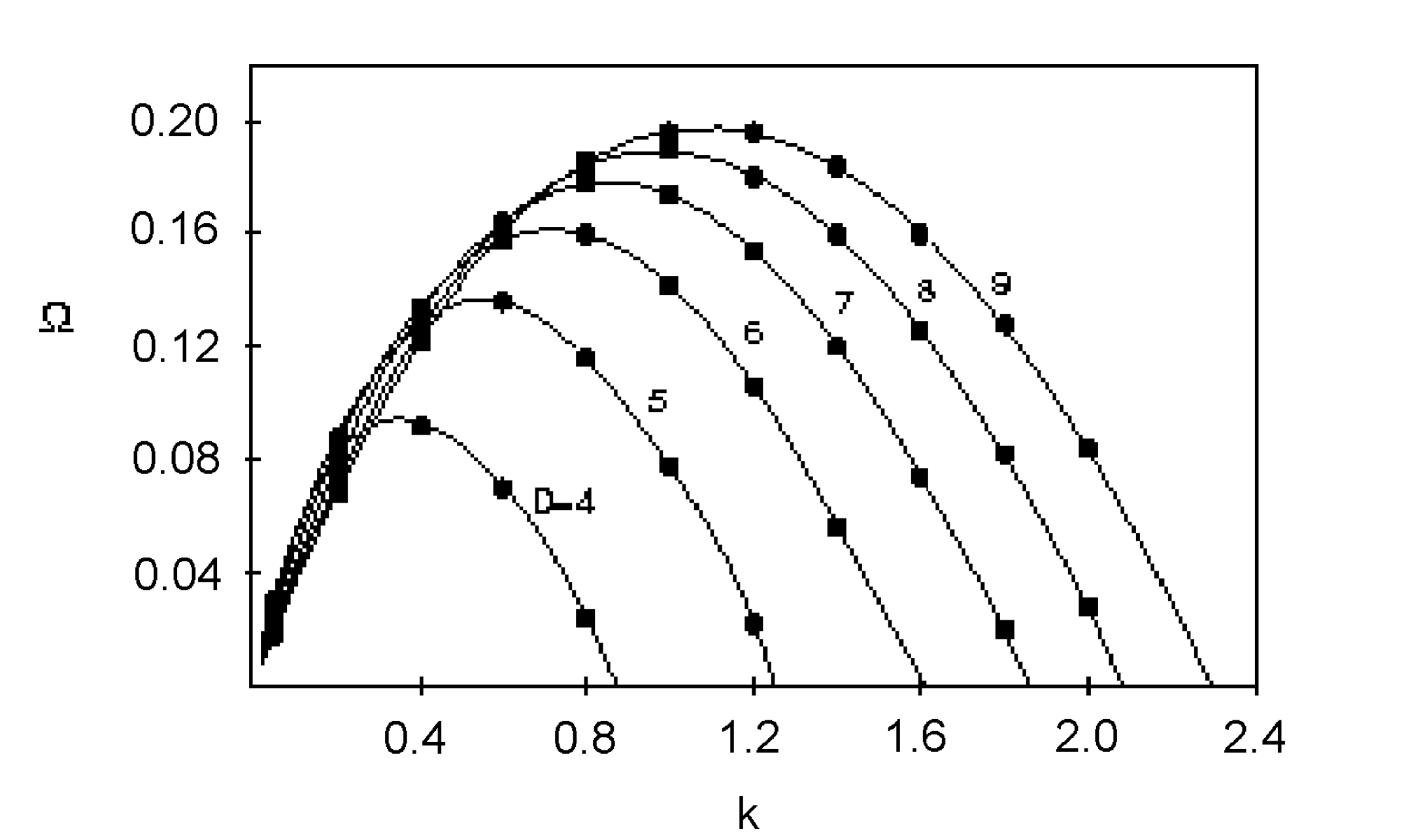
Figure 1: The Gregory-Laflamme $\Omega(k)$ curve in $d$ dimensions reprinted from Ref. [2], where $D|_{\rm figure}=d$ used in this review.

Figure 1 reveals that the curve of possible values of $\Omega$ and $k$ intersects the $k$-axis in two places: $k=0$ and $k=k_{c}$, where $k_{c}$ is a critical non-zero wave-number. The fact that the curve does not intersect the $k$-axis at $k<0$ follows from the stability of the Schwarzschild-Tangherlini black hole (otherwise we would have an unstable mode with $\Omega>0$ and $k=0$). On the other hand, the presence of an intersection at $k=k_{c}$ is a signature of a long wavelength instability: it means that there is an unstable mode for any wavelength larger than the critical wavelength

$$\lambda_{\rm GL}=\frac{2\pi r_{0}}{k_{c}}~{}.$$ (2.14)

The critical wave-number $k_{c}$ marks the lower bound of the possible wavelengths for which there is an unstable mode. Therefore, we call the mode with $k=k_{c}$ and $\Omega=0$ the threshold mode. It is a time-independent mode of the form

$$h_{c,\mu\nu}=\Re\left\{\exp\left(i\frac{k_{c}z}{r_{0}}\right)P_{c,\mu\nu}\right\}$$ (2.15)

As we shall see in the following, the threshold mode is important for several reasons:

• It signals the instability of the black string itself.

• It can be mapped to unstable modes for other gravity solutions.

• It suggests the existence of a static non-uniform black string.

Below, we go through each of these different aspects of the threshold mode. The values of $k_{c}$ for $d=4,...,14$, as obtained in [2, 29, 31], are listed in Table 1.

$d$	$4$	$5$	$6$	$7$	$8$	$9$	$10$	$11$	$12$	$13$	$14$
$k_{c}$	$0.88$	$1.24$	$1.60$	$1.86$	$2.08$	$2.30$	$2.50$	$2.69$	$2.87$	$3.03$	$3.18$

Table 1: The critical wave numbers $k_{c}$ for the Gregory-Laflamme instability.

2.2.2 The Lichnerowitz operator and the threshold mode

The fact that the mode (2.11)-(2.12) solves the Einstein equations as a perturbation can be formulated in the following way. Define the Lichnerowitz operator for a background metric $g_{\mu\nu}$ as

$$(\Delta_{L})_{\mu\nu\rho\sigma}=-g_{\mu\rho}g_{\nu\sigma}D_{\kappa}D^{\kappa}-2R_{\mu\nu\rho\sigma}$$ (2.16)

Here $L$ refers to Lorentzian signature. In the ensuing it will be convenient to use the short-hand notation

$$\Delta_{L}h_{\mu\nu}\equiv{(\Delta_{L})_{\mu\nu}}^{\rho\sigma}h_{\rho\sigma}~{}.$$ (2.17)

Then, the statement that the perturbation $h_{\mu\nu}$ of $g_{\mu\nu}$ satisfies the Einstein equations of motion can be stated as the differential operator equation

$$\Delta_{L}h_{\mu\nu}=0$$ (2.18)

Hence what appears in Appendix A is a check that the perturbation (2.11)-(2.12) satisfies the Lichnerowitz equation (2.18), with (2.9) as the background metric. We can write the relevant equations more explicitly as

$${(\Delta_{L})_{\mu\nu}}^{\rho\sigma}\left(P_{\rho\sigma}e^{\Omega t/r_{0}}e^{ikz/r_{0}}\right)=0$$ (2.19)

In this expression, $P_{\mu\nu}$ has no explicit dependence on $t$ and $z$ and $P_{z\mu}=0$ for all $\mu$. Since the background metric (2.9) has $g_{zz}=1$, we deduce that we can rewrite (2.19) as

$${(\hat{\Delta}_{L})_{\mu\nu}}^{\rho\sigma}\left(P_{\rho\sigma}e^{\Omega t/r_{0}}\right)=-\frac{k^{2}}{r_{0}^{2}}P_{\mu\nu}e^{\Omega t/r_{0}}$$ (2.20)

where $\hat{\Delta}_{L}$ is the dimensionally reduced Lichnerowitz operator arising from the metric in one dimension less, $i.e.$ with the $z$-direction excluded. In particular, for the threshold mode with $\Omega=0$ and $k=k_{c}$

$$\hat{\Delta}_{L}P_{c,\mu\nu}=-\frac{k_{c}^{2}}{r_{0}^{2}}P_{c,\mu\nu}~{}.$$ (2.21)

This expression has taken the form of an eigenvalue equation for the dimensionally reduced Lichnerowitz operator $\hat{\Delta}_{L}$. In general, one could look for all possible solutions to the eigenvalue equation

$$\hat{\Delta}_{L}U_{\mu\nu}=\alpha U_{\mu\nu}$$ (2.22)

thus obtaining the full spectrum of eigenvalues $\alpha$ of the Lichnerowitz operator. It is now clear from (2.21) that the existence of the threshold mode is equivalent to the existence of a negative eigenvalue for the dimensionally reduced Lichnerowitz operator ${\hat{\Delta}}_{L}$. Taking the existence of the threshold mode as a signal for the existence of the unstable Gregory-Laflamme mode, we deduce that a negative eigenvalue of the dimensionally reduced Lichnerowitz operator is a signal of a long wavelength instability for the solution. This statement will be important in Section 6.1.

2.2.3 Comparison with Jeans instability

Is there any relation or analogy between the Gregory-Laflamme instability of neutral black strings and the Jeans instability of a massive object with similar physical properties such as dimension and mass? For example, does such an object have a Jeans Instability that sets in at approximately the same point as the Gregory-Laflamme instability? To see such an analogy, we note that the black string in a $d+1$ dimensional flat space-time has mass per unit length $M/L\sim r_{0}^{d-3}/G$. From this we deduce that the mass density is $\rho_{0}\sim M/(Lr_{0}^{d-1})\sim 1/(Gr_{0}^{2})$. Thus, for a system with these physical parameters (2.8) implies that the Jeans instability should set in at wavelengths larger than the critical wavelength

$$\lambda_{J}\sim\frac{1}{\sqrt{G\rho_{0}}}\sim r_{0}$$ (2.23)

where we take the velocity of sound to be the speed of light. So, indeed there is a Jeans instability that sets in when $\lambda/r_{0}$ is larger than some number of order one. This is in good qualitative agreement with the Gregory-Laflamme instability, which sets in at wavelengths larger than the critical wavelength $\lambda_{\rm GL}=2\pi r_{0}/k_{c}$ where $k_{c}$ is a number of order one given in Table 1.

It is interesting to push this correspondence between the Gregory-Laflamme instability and the Jeans Instability even further to the large dimension limit $d\rightarrow\infty$, especially since the gravitational field behaves in a Newtonian fashion in this limit. Keeping track of the $d$-dimensional factors in the derivation above, one finds for $d\gg 1$ that $\lambda_{J}\sim d^{-3/4}r_{0}$. As we will see in Section 4.1, this critical wavelength does not have the right asymptotic behavior compared to the one found for the GL mode. Interestingly, however, the (classical) Rayleigh-Plateau instability reviewed in Section 4.4 does predict the correct asymptotic behavior [36].

2.2.4 Gregory-Laflamme instability for the compactified neutral black string

We have discussed the neutral black string solution in $D$ dimensional Minkowski space. However, for many reasons it is more meaningful to consider instead the neutral black string in a space-time with a compact direction parallel to the string. For one thing, the question of the end point of the black string instability becomes in this setting a more well-defined problem. Moreover, the fact that the string is wrapped on a circle allows us to stabilize it by making the circle smaller than the critical Gregory-Laflamme wavelength, so that the Gregory-Laflamme mode cannot fit into the geometry. In what follows, we briefly analyze the neutral black string in a Kaluza-Klein space-time. Later in Section 3 we will put this into the more general context of Kaluza-Klein black holes.

To this end, consider the neutral black string solution (2.9) with a periodic $z$ coordinate whose period we will denote by $L$. This solution describes a neutral black string in a $D=d+1$ dimensional Kaluza-Klein space-time $\mathcal{M}^{d}\times S^{1}$. Indeed, the black string solution (2.9) asymptotes to $\mathcal{M}^{d}\times S^{1}$ as $r\rightarrow\infty$. Henceforth we shall denote this solution as the (compactified) neutral uniform black string solution, in order to distinguish it from another branch of black string solutions that will be discussed later. The mass of the compactified neutral uniform black string is

$$M=\frac{\Omega_{d-2}L}{16\pi G}(d-2)r_{0}^{d-3}~{}.$$ (2.24)

It is useful to define a rescaled mass which is dimensionless, using the circumference $L$:

$$\mu\equiv\frac{16\pi G}{L^{d-2}}M~{}.$$ (2.25)

Then for the compactified neutral uniform black string we have

$$\mu=(d-2)\Omega_{d-2}\left(\frac{r_{0}}{L}\right)^{d-3}~{}.$$ (2.26)

We see that the Gregory-Laflamme mode (2.11)-(2.12) cannot obey the correct periodic boundary condition on $z$ if $L<\lambda_{\rm GL}$, with $\lambda_{\rm GL}$ given by (2.14). On the other hand, for $L>\lambda_{\rm GL}$, we can fit the Gregory-Laflamme mode into the compact direction with the frequency and wave number $\Omega$ and $k$ in (2.11)-(2.12) determined by the ratio $r_{0}/L$. Translating this in terms of the mass of the neutral black string (2.26), we deduce that we have a critical Gregory-Laflamme mass given by

$$\mu_{\rm GL}=(d-2)\Omega_{d-2}\left(\frac{k_{c}}{2\pi}\right)^{d-3}~{}.$$ (2.27)

For $\mu<\mu_{\rm GL}$ the Gregory-Laflamme mode can be fitted into the circle, and the compactified neutral uniform black string is unstable. For $\mu>\mu_{\rm GL}$, on the other hand, the Gregory-Laflamme mode is absent, and the neutral uniform black string is stable. For $\mu=\mu_{\rm GL}$ there is a marginal mode which, as we discuss below, signals the emergence of a new branch of black string solutions which are non-uniformly distributed along the circle. In Table 2 we record the critical Gregory-Laflamme mass $\mu_{\rm GL}$ that follows from the numerical data of Table 1 (obtained in [2, 29, 31]) using (2.27).

$d$	$4$	$5$	$6$	$7$	$8$	$9$	$10$	$11$	$12$	$13$	$14$
$\mu_{\rm GL}$	$3.52$	$2.31$	$1.74$	$1.19$	$0.79$	$0.55$	$0.37$	$0.26$	$0.18$	$0.12$	$0.08$

Table 2: The critical masses $\mu_{\rm GL}$ for the Gregory-Laflamme instability.

As we mentioned above, for the compactified neutral uniform black string we can meaningfully ask about the end-point of the instability of the string for $\mu<\mu_{\rm GL}$. We will discuss this question further in Section 3.2. One of the problematic issues regarding the question about the end-point of the Gregory-Laflamme instability in the uncompactified uniform black string case is the infinite mass of the black string. If the instability ended, for example, with a breaking up of the horizon into disconnected pieces, there would have to be an infinite process of localized instabilities happening one after another without end. This process is regularized in the compactified case and therefore it seems more sensible to consider the instability of the neutral black string in the compactified setting.

2.2.5 Neutral non-uniform black strings

Let us re-consider now the threshold mode, $i.e.$ the critical Gregory-Laflamme mode with $\Omega=0$ and $k=k_{c}$. This mode obeys the equation (2.21), or equivalently the equation

$${(\Delta_{L})_{\mu\nu}}^{\rho\sigma}\left(P_{c,\rho\sigma}e^{ik_{c}z/r_{0}}\right)=0~{}.$$ (2.28)

$P_{c,\mu\nu}e^{ik_{c}z/r_{0}}$ is a marginal mode that depends explicitly on the compact direction $z$. Therefore, as noticed in [28, 29, 30], the mode corresponds to a new static classical solution that can be seen as a neutral black string with a horizon that is non-uniform in the $z$ direction. In other words, the mode signals the emergence of a new branch of black string solutions which are non-uniformly distributed along the circle. We will call this branch of solutions non-uniform black strings, as opposed to the uniform black string solutions (2.9). In section 3 we review the properties of the finitely deformed non-uniform black string solution that has been found numerically, and the connection with other branches in the full phase diagram of solutions. Note that the topology of the horizon is $S^{d-2}\times S^{1}$ for both the uniform as well as the non-uniform black string (in the compactified case).

2.2.6 Manifestations of the Gregory-Laflamme mode

The Gregory-Laflamme mode discussed above shows up in many different set ups in black hole physics, all connected to the question of stability. In the following, we describe briefly various implications and manifestations of the Gregory-Laflamme mode and the context in which they appear:

• Neutral non-uniform black string branch. This is described above in this section. Here the threshold mode corresponds to a static black string solution which is non-uniform along the direction of the string.

• Instability of static Kaluza-Klein bubble. This will be discussed below in Section 2.3. In this context the threshold mode is double-Wick-rotated into an unstable mode for the static Kaluza-Klein bubble.

• Semi-classical black hole instability in the canonical ensemble. Consider the 5D threshold mode (2.21), involving the dimensionally reduced 4D Lichnerowicz operator ${\hat{\Delta}}_{L}$. By Wick rotating the mode, we obtain an eigenmode $u_{\mu\nu}$ for the Lichnerowitz operator $\Delta_{\rm E}$ of the Euclidean section of the 4D Schwarzschild black hole with eigenvalue $-k_{c}^{2}r_{0}^{-2}$. Using the relation $r_{0}=2G_{4}M$, where $G_{4}$ is four-dimensional Newton’s constant and $M$ the four-dimensional mass, we deduce that $u_{\mu\nu}$ obeys the equation

  $$\Delta_{\rm E}u_{\mu\nu}=-0.19(G_{4}M)^{-2}u_{\mu\nu}$$ (2.29)

  where we used the value $k_{c}=0.88$ from Table 1. This is precisely the eigenmode for the Euclidean section of the 4D Schwarzschild black hole found by Gross, Perry, and Yaffe in [89]. In [89] it was argued as a consequence of the mode (2.29) that the Euclidean flat space $\mathbb{R}^{3}\times S^{1}$ (hot flat space) is semi-classically unstable to nucleation of Schwarzschild black holes. In other words, for any non-zero temperature it is thermodynamically preferred for a gas of gravitons in Minkowski space to form a black hole. It is easily seen using the higher-dimensional threshold modes that this can be extended to higher dimensions, $i.e.$ that hot flat space $\mathbb{R}^{d}\times S^{1}$ is unstable to nucleation of $(d+1)$-dimensional Schwarzschild-Tangherlini black holes.

• Local thermodynamic instability. In [64] it was shown, following the conjectures of [62, 63], that a Euclidean negative mode implies a local thermodynamic instability, and vice versa. For the Schwarzschild black hole this is clearly the case since the heat capacity is negative. If there is in addition a flat non-compact direction one can Wick rotate the Euclidean mode to a threshold Gregory-Laflamme mode, implying that classical instability for black branes with non-compact directions is in correspondence with local thermodynamic instability. We explain and review this topic in Section 6.

• Gregory-Laflamme modes for charged branes. Finally, one can also map the neutral Gregory-Laflamme mode to Gregory-Laflamme modes for charged branes [56, 66]. Moreover, in [66] it is shown that the Gregory-Laflamme modes in the limit $(k,\Omega)\rightarrow(0,0)$ become marginal modes for extremal branes uniformly smeared along a transverse direction. We review and discuss these issues in Section 5.

2.3 Instability of the static Kaluza-Klein bubble

Kaluza-Klein bubbles were discovered in [90] by Witten. In [90] it was explained that the Kaluza-Klein vacuum $\mathcal{M}^{4}\times S^{1}$ is unstable semi-classically, at least in the absence of fundamental fermions. The semi-classical instability of $\mathcal{M}^{4}\times S^{1}$ proceeds through the spontaneous creation of expanding Kaluza-Klein bubbles, which are Wick rotated 5D Schwarzschild-Tangherlini black hole solutions. The Kaluza-Klein bubble is essentially a minimal $S^{2}$ somewhere in the space-time, $i.e.$ a “bubble of nothing”. In the expanding Kaluza-Klein bubble solution the $S^{2}$ bubble expands until all of the space-time is gone. However, apart from these time-dependent bubble solutions there are also solutions with static bubbles, as we now review.

To construct the static Kaluza-Klein bubble in $d+1$ dimensions we take the metric (2.9) of the neutral uniform black string and make a double Wick-rotation in the $t$ and $z$ directions. After a convenient relabeling, we obtain the metric

$$ds^{2}=-dt^{2}+\left(1-\frac{R^{d-3}}{r^{d-3}}\right)dz^{2}+\frac{1}{1-\frac{R^{d-3}}{r^{d-3}}}dr^{2}+r^{2}d\Omega_{d-2}^{2}\ .$$ (2.30)

We see that there is a minimal $(d-2)$-sphere of radius $R$ located at $r=R$. To avoid a conical singularity we need to make $z$ a periodic coordinate with period

$$L=\frac{4\pi R}{d-3}\ .$$ (2.31)

Clearly, the solution asymptotes to $\mathcal{M}^{d}\times S^{1}$ for $r\rightarrow\infty$. Notice that the only free parameter in the solution is the circumference of the $S^{1}$.

The static Kaluza-Klein bubble is classically unstable. This can be seen using the threshold Gregory-Laflamme mode (2.21). After a double Wick-rotation $t\rightarrow iz$, $z\rightarrow it$ of the threshold mode, we obtain a mode $U_{\mu\nu}$ obeying $\Delta U_{\mu\nu}=-k_{c}^{2}R^{-2}U_{\mu\nu}$, where $\Delta$ is the Lichnerowitz operator for the static Kaluza-Klein bubble (2.30). Using that $g_{tt}=-1$ in (2.30) we deduce that

$${\Delta_{\mu\nu}}^{\rho\sigma}\left(U_{\rho\sigma}e^{\pm k_{c}R^{-1}t}\right)=0$$ (2.32)

Hence, $U_{\rho\sigma}e^{\pm k_{c}R^{-1}t}$ corresponds to an unstable mode for the static Kaluza-Klein bubble (2.30), implying that the static Kaluza-Klein bubble is classically unstable to small s-wave perturbations.

The classical instability of the static Kaluza-Klein bubble causes the bubble to either expand or collapse exponentially fast. For five-dimensional Kaluza-Klein space-times, there exist initial data [92] for massive bubbles that are initially expanding or collapsing [93], and numerical studies [94] show that there exist massive expanding bubbles and furthermore indicate that contracting massive bubbles collapse to a black hole with an event horizon. In the latter case, it is noteworthy that the value of $\mu$ in (3.20) is smaller than $\mu_{\rm GL}$, the Gregory-Laflamme mass, for $4\leq d\leq 9$ (as can be seen by comparing $\mu_{\rm b}$ in (3.20) to $\mu_{\rm GL}$ in Table 3). This implies that the static Kaluza-Klein bubble does not decay to the uniform black string. It is therefore likely that the Kaluza-Klein bubble in that case decays to whatever is the endstate of the uniform black string (see end of Section 3.2).

Finally, we note that in Ref. [95] charged bubble solutions were constructed that are perturbatively stable, though it was argued that these are non-perturbatively unstable. These bubble solutions play a role in the end state of tachyon condensation of charged black strings.

3 Phases of Kaluza-Klein black holes

In the previous section we focused primarily on the uniform black string and its GL instability. In this section we turn to a more general description of the phases of Kaluza-Klein black holes. A $(d+1)$-dimensional Kaluza-Klein black hole will be defined here as a pure gravity solution with at least one event horizon that asymptotes to $d$-dimensional Minkowski space times a circle ($\mathcal{M}^{d}\times S^{1}$) at infinity. We will discuss only static and neutral solutions, $i.e.$ solutions without charges and angular momenta. Obviously, the uniform black string is an example of a Kaluza-Klein black hole, but many more phases are known to exist. In this section, we present their properties as well as the possible relation of these phases to the GL instability (see also the shorter review [96]).

3.1 Physical parameters and definition of the phase diagram

In this subsection we present a general method of computing the mass $\mu$ and relative tension $n$ of a Kaluza-Klein black hole, which will be later used to plot each phase in a $(\mu,n)$ phase diagram. We review the main features of the split-up of this phase diagram into two regions. Finally, we discuss some general results on the thermodynamics of Kaluza-Klein black holes.

3.1.1 Computing the mass and tension

For any space-time which asymptotes to $\mathcal{M}^{d}\times S^{1}$ we can define the mass $M$ and the tension $\mathcal{T}$. These quantities can be used to parameterize the various phases of Kaluza-Klein black holes, as we review below.

Let us define the Cartesian coordinates for $d$-dimensional Minkowski space $\mathcal{M}^{d}$ as $t,x^{1},...,x^{d-1}$ and the radius $r=\sqrt{\sum_{i}(x^{i})^{2}}$. In addition we use a coordinate $z$ of period $L$ to label the $S^{1}$. Hence, the total space-time dimension is $D=d+1$. In this notation, we have for any localized static object the asymptotics [47]

$$g_{tt}\simeq-1+\frac{c_{t}}{r^{d-3}}\ ,\ \ g_{zz}\simeq 1+\frac{c_{z}}{r^{d-3}}\ ,$$ (3.1)

as $r\rightarrow\infty$. The mass $M$ and tension $\mathcal{T}$ are then given by [47, 48]

$$M=\frac{\Omega_{d-2}L}{16\pi G_{\rm N}}\left[(d-2)c_{t}-c_{z}\right]\ ,\ \ \mathcal{T}=\frac{\Omega_{d-2}}{16\pi G_{\rm N}}\left[c_{t}-(d-2)c_{z}\right]\ .$$ (3.2)

The tension in (3.2) can also be obtained from the general formula for tension in terms of the extrinsic curvature [97] analogous to the Hawking-Horowitz mass formula [98]. The mass and tension formulas have been generalized to non-extremal and near-extremal branes in [57]. Gravitational tension for black branes has also been considered in [99, 100, 101].

In what follows, it will be convenient to define the relative tension (also called the relative binding energy) as [47]

$$n=\frac{\mathcal{T}L}{M}=\frac{c_{t}-(d-2)c_{z}}{(d-2)c_{t}-c_{z}}\ .$$ (3.3)

This ratio provides a measure of how large the tension (or binding energy) is relative to the mass. It is a useful quantity because it is dimensionless and bounded as [47]

$$0\leq n\leq d-2\ .$$ (3.4)

The upper bound is due to the Strong Energy Condition whereas the lower bound was found in [102, 103]. The upper bound can also be understood physically in a more direct way from the fact that we expect gravity to be an attractive force. For a test particle at infinity it is easy to see that the gravitational force on the particle is attractive when $n<d-2$ but repulsive when $n>d-2$.

It is also useful to define a rescaled dimensionless quantity from the mass as

$$\mu=\frac{16\pi G_{\rm N}}{L^{d-2}}M\ .$$ (3.5)

The program set forth in [47, 49] is to plot all phases of Kaluza-Klein black holes in a $(\mu,n)$ diagram. We shall turn to this in the following.

3.1.2 The split-up of the phase diagram

According to the present knowledge of the phases of static and neutral Kaluza-Klein black holes, the $(\mu,n)$ phase diagram appears to be divided into two separate regions [50]:

• The region $0\leq n\leq 1/(d-2)$ contains solutions without Kaluza-Klein bubbles, and the solutions have a local $SO(d-1)$ symmetry. We review what is known about solutions in this part of the phase diagram in Section 3.2. Because of the $SO(d-1)$ symmetry there are only two types of event horizon topologies: $S^{d-1}$ for the black hole on a cylinder branch and $S^{d-2}\times S^{1}$ for the black string.

• The region $1/(d-2)<n\leq d-2$ contains solutions with Kaluza-Klein bubbles. We review this class of solutions in Section 3.3. This part of the phase diagram, which is much more densely populated with solutions compared to the lower part, is the subject of [50].

3.1.3 Thermodynamics, first law and the Smarr formula

For a neutral Kaluza-Klein black hole with a single connected horizon, we can find the temperature $T$ and entropy $S$ directly from the metric. Together with the mass $M$ and tension ${\cal{T}}$, these quantities obey the Smarr formula [47, 48]

$$(d-1)TS=(d-2)M-L{\cal{T}}$$ (3.6)

and the first law of thermodynamics [101, 48, 49]

$$\delta M=T\delta S+{\cal{T}}\delta L~{}.$$ (3.7)

This equation includes a “work” term (analogous to $p\delta V$) for variations with respect to the size of the circle at infinity. See $e.g.$ Ref. [49] for a proof of the first law based on the Smarr formula (3.6) using an ansatz (see (3.11) below) for black holes/strings on cylinders and a class of static Ricci-flat perturbations. See also Ref. [104] for a more general proof based on Hamiltonian methods.

It is useful to define the rescaled temperature $\mathfrak{t}$ and entropy $\mathfrak{s}$ as

$$\mathfrak{t}=LT\ ,\ \ \mathfrak{s}=\frac{16\pi G_{\rm N}}{L^{d-1}}S\ .$$ (3.8)

In terms of these quantities, the Smarr formula for Kaluza-Klein black holes and the first law of thermodynamics take the form

$$(d-1)\mathfrak{t}\mathfrak{s}=(d-2-n)\mu\ ,\ \ \delta\mu=\mathfrak{t}\,\delta\mathfrak{s}\ .$$ (3.9)

Combining the Smarr formula and the first law, we get the relation

$$\frac{\delta\log\mathfrak{s}}{\delta\log\mu}=\frac{d-1}{d-2-n}\ ,$$ (3.10)

so that, given a curve $n(\mu)$ in the phase diagram, the entire thermodynamics can be obtained.

From (3.10) it is also possible to derive the Intersection Rule of [47]: for two branches that intersect at the same solution, the branch with the lower relative tension has the highest entropy for masses below the intersection point, whereas the branch with the higher relative tension has the highest entropy for masses above the intersection point. An illustration of the Intersection Rule appears in Figure 2.

Figure 2: Illustration of the Intersection Rule.

It is important to note that there are also examples of Kaluza-Klein black hole solutions with more than one connected event horizon [49, 50, 105]. The Smarr formula and first law of thermodynamics generalize also to these cases.

3.2 Black holes and strings on cylinders

In this subsection we review the properties of neutral and static black objects without Kaluza-Klein bubbles. These turn out to have local $SO(d-1)$ symmetry, which implies that the solutions fall into two categories, black holes with event horizon topology $S^{d-1}$ and black strings with event horizon topology $S^{d-2}\times S^{1}$. First we discuss the ansatz that follows from the local $SO(d-1)$ symmetry. Then we review the uniform black string, non-uniform black string and localized black hole phases. These phases are drawn in the $(\mu,n)$ phase diagram for the five- and six-dimensional cases. Finally we consider various related topics, including the existence of copies of solutions, the endpoint of the decay of the uniform black string and an observation related to the large $d$ behavior.

3.2.1 The ansatz

As we mentioned above, all solutions with $0\leq n\leq 1/(d-2)$ have, to our present knowledge, a local $SO(d-1)$ symmetry. Using this symmetry it has been shown [51, 49] that the metric of these solutions can be written in the form

$$ds^{2}=-fdt^{2}+\frac{L^{2}}{(2\pi)^{2}}\left[\frac{A}{f}dR^{2}+\frac{A}{K^{d-2}}dv^{2}+KR^{2}d\Omega_{d-2}^{2}\right]\ ,\ \ f=1-\frac{R_{0}^{d-3}}{R^{d-3}}\ ,$$ (3.11)

where $R_{0}$ is a dimensionless parameter, $R$ and $v$ are dimensionless coordinates and the metric is determined by the two functions $A=A(R,v)$ and $K=K(R,v)$. The form (3.11) was originally proposed in Refs. [38, 106] as an ansatz for the metric of black holes on cylinders.

The properties of the ansatz (3.11) were extensively considered in [38]. It was found that the function $A=A(R,v)$ can be written explicitly in terms of the function $K(R,v)$ thus reducing the number of free unknown functions to one. The functions $A(R,v)$ and $K(R,v)$ are periodic in $v$ with the period $2\pi$. Note that $R=R_{0}$ is the location of the horizon in (3.11).

As already stated, all phases without Kaluza-Klein bubbles have, to our present knowledge, $0\leq n\leq 1/(d-2)$ and can be described by the ansatz (3.11). In what follows we review the three known phases in this class and describe their properties.

3.2.2 Uniform string branch

The uniform string branch consists of neutral black strings which are translationally invariant along the circle direction. The metric of a uniform string in $d+1$ dimensions is [12]

$$ds^{2}=-\left(1-\frac{r_{0}^{d-3}}{r^{d-3}}\right)dt^{2}+\left(1-\frac{r_{0}^{d-3}}{r^{d-3}}\right)^{-1}dr^{2}+r^{2}d\Omega_{d-2}^{2}+dz^{2}\ .$$ (3.12)

As we can see easily from the metric (3.12) using (3.1) and (3.3), the relative binding energy is $n=1/(d-2)$ for the whole uniform string branch. Hence, the uniform string branch is a horizontal line in the $(\mu,n)$ diagram. The rescaled entropy is given by the expression

$$\mathfrak{s}_{\rm u}(\mu)=C_{1}^{(d-1)}\mu^{\frac{d-2}{d-3}}\ ,$$ (3.13)

where the constant $C_{1}^{(q)}$ is defined as

$$C_{1}^{(q)}\equiv 4\pi(\Omega_{q-1})^{-\frac{1}{q-2}}(q-1)^{-\frac{q-1}{q-2}}\ .$$ (3.14)

The horizon topology of the uniform black string is clearly $S^{1}\times S^{d-2}$, where the $S^{1}$ is along the circle-direction.

The most important physical feature of the neutral uniform black string solution is the GL instability reviewed in Section 2.2. As stated there, a compactified neutral uniform black string is classically unstable for $\mu<\mu_{\rm GL}$, $i.e.$ it is unstable for sufficiently small masses. See Table 2 for the numerical values of the critical mass $\mu_{\rm GL}$ when $d\leq 14$. For $\mu>\mu_{\rm GL}$ the string is believed to be classically stable. We comment on the endpoint of the classical instability of the uniform black string below.

3.2.3 Non-uniform string branch

It was realized in [29] that the classical instability of the uniform black string for $\mu<\mu_{\rm GL}$ implies the existence of a marginal mode at $\mu=\mu_{\rm GL}$, which again suggests the existence of a new branch of solutions. Since the new branch of solutions is continuously connected to the uniform black string it is expected to have the same horizon topology, at least when the deformation away from the uniform black string is sufficiently small. Moreover, the solution is expected to be non-uniformly distributed in the circle-direction $z$ since there is an explicit dependence in the marginal mode on this direction.

The new branch, which we call here the non-uniform string branch, has been found numerically in [29, 30, 31]. Its most prominent features are:

• The horizon topology is $S^{1}\times S^{d-2}$ with the $S^{1}$ being the circle of the Kaluza-Klein space-time $\mathcal{M}^{d}\times S^{1}$.

• The solutions are non-uniformly distributed along $z$.

• The non-uniform black strings have a local $SO(d-1)$ symmetry and therefore can be written in terms of the ansatz (3.11) [51, 49].

• The non-uniform string branch meets the uniform string branch at $\mu=\mu_{\rm GL}$ on the line with $n=1/(d-2)$.

• The branch has relative tension $n<1/(d-2)$.

More concretely, considering the non-uniform black string branch for $|\mu-\mu_{\rm GL}|\ll 1$ one obtains

$$n(\mu)=\frac{1}{d-2}-\gamma(\mu-\mu_{\rm GL})+\mathcal{O}((\mu-\mu_{\rm GL})^{2})\ .$$ (3.15)

Here $\gamma$ is a number representing the slope of the curve that describes the non-uniform string branch near $\mu=\mu_{\rm GL}$. The numerical data for $\mu_{\rm GL}$ when $4\leq d\leq 14$ are given in Table 2 and the corresponding results for $\gamma$ in Table 3. These data were computed in [2, 3, 29, 30, 31].

$d$	$4$	$5$	$6$	$7$	$8$	$9$	$10$	$11$	$12$	$13$	$14$
$\gamma$	$0.14$	$0.17$	$0.21$	$0.31$	$0.47$	$0.74$	$1.4$	$2.8$	$7.9$	$-40$	$-9.2$

Table 3: The constant $\gamma$ which, together with $\mu_{\rm GL}$ of Table 2, determines the behavior of the non-uniform branch for $|\mu-\mu_{\rm GL}|\ll 1$ .

The large $d$ behavior of $\mu_{\rm GL}$ was examined numerically in [31] and analytically in [35]. The latter will be discussed in Section 4.1.

The qualitative behavior of the non-uniform string branch depends on the sign of $\gamma$. If $\gamma$ is positive, then the branch emerges at the mass $\mu=\mu_{\rm GL}$ with increasing $\mu$ and decreasing $n$. If instead $\gamma$ is negative the branch emerges at $\mu=\mu_{\rm GL}$ with decreasing $\mu$ and decreasing $n$. One can use the Intersection Rule of [47] (see Section 3.1) to see that if $\gamma$ is positive (negative) then the entropy of the uniform string branch for a given mass is higher (lower) than the entropy of the non-uniform string branch for that mass. This result can also be derived directly from (3.15) using (3.10). We find

$$\frac{\mathfrak{s}_{\rm nu}(\mu)}{\mathfrak{s}_{\rm u}(\mu)}=1-\frac{(d-2)^{2}}{2(d-1)(d-3)^{2}}\frac{\gamma}{\mu_{\rm GL}}(\mu-\mu_{\rm GL})^{2}+\mathcal{O}((\mu-\mu_{\rm GL})^{3})\ ,$$ (3.16)

from which we clearly see the significance of the sign of the parameter $\gamma$. In this expression $\mathfrak{s}_{\rm u}(\mu)$ ($\mathfrak{s}_{\rm nu}(\mu)$) refers to the rescaled entropy of the uniform (non-uniform) black string branch. From the data of Table 3 we see that $\gamma$ is positive for $d\leq 12$ and negative for $d\geq 13$ [31]. Therefore, as discovered in [31], the non-uniform black string branch has a qualitatively different behavior for small $d$ and large $d$, $i.e.$ the system exhibits a critical dimension $D=14$.

Numerical results

In six dimensions, $i.e.$ for $d=5$, Wiseman found in [30] a large body of numerical data for the non-uniform string branch. These data are displayed in the $(\mu,n)$ phase diagram on the right side of Figure 3 [47]. The branch starts at $\mu=\mu_{\rm GL}$ and the data end around $\mu\simeq 2.3\,\mu_{\rm GL}\simeq 5.3$. In [46] numerical evidence has been found that suggests that the non-uniform string branch more or less ends where the data of [30] end, $i.e.$ around $\mu\simeq 5.3$ for $d=5$, supporting the considerations of [52]. Recently, numerical results extending the non-uniform branch into the strongly non-linear regime were also obtained for the case of five dimensions, $i.e.$ for $d=4$, in Ref. [32], and for the entire range $d\leq 5\leq 10$ in Ref. [33]. All these non-uniform black string solutions have masses above the GL mass and less entropy than the corresponding uniform black string.

Another interesting feature of the non-uniform solutions is the local geometry around the “waist” of the most non-uniform solutions. This is cone-like to a fairly good approximation [52, 33], lending support to the ideas proposed in [34, 68] (see also Section 4.4). As we further discuss below, all these data provide important evidence that the non-uniform branch has a topology changing transition into the localized black hole branch.

3.2.4 Localized black hole branch

On physical grounds, it is natural to expect a branch of neutral black holes in the space-time $\mathcal{M}^{d}\times S^{1}$. One defining feature of these solutions is an event horizon of topology $S^{d-1}$. We will call this branch the localized black hole branch in the following, because the $S^{d-1}$ horizon is localized on the $S^{1}$ of the Kaluza-Klein space.

Neutral black hole solutions in the space-time $\mathcal{M}^{3}\times S^{1}$ were found and studied in [107, 108, 109, 110]. However, the study of black holes in the space-time $\mathcal{M}^{d}\times S^{1}$ for $d\geq 4$ has begun only recently. The complexity of the problem stems from the fact that such black holes are not algebraically special [111] and moreover from the fact that the solution cannot be found using a Weyl ansatz since the number of Killing vectors is too small.

Analytical results

Progress towards finding an analytical solution for the localized black hole was made in [38] where, as reviewed above, the ansatz (3.11) was proposed. Subsequently it was proven in [51, 49] that the localized black hole can be put in this ansatz.

In [39] the metric of small black holes, $i.e.$ black holes with mass $\mu\ll 1$, was found analytically using the ansatz (3.11) of [38] to first order in $\mu$. Subsequently, an equivalent expression for the first order metric was found in Refs. [40, 41] using a different method. An important feature of the localized black hole solution is the fact that $n\rightarrow 0$ as $\mu\rightarrow 0$. This means that the black hole solution becomes more and more like a $(d+1)$-dimensional Schwarzschild black hole as the mass goes to zero. For $d=4$, the second order correction to the metric and thermodynamics have recently been studied in [42]. More generally, the second order correction to the thermodynamics was obtained in Ref. [43] for all $d$ using an effective field theory formalism in which the structure of the black hole is encoded in the coefficients of operators in an effective worldline Lagrangian.

The first order result of [39] and second order result of [43] can be summarized by giving the first and second order corrections to the relative tension $n$ of the localized black hole branch as a function of $\mu$

$$n=\frac{(d-2)\zeta(d-2)}{2(d-1)\Omega_{d-1}}\mu-\left(\frac{(d-2)\zeta(d-2)}{2(d-1)\Omega_{d-1}}\mu\right)^{2}+\mathcal{O}(\mu^{3})\ .$$ (3.17)

Plugging this expression into (3.10) one can find the leading correction to the thermodynamics as

$$\mathfrak{s}_{\rm bh}(\mu)=C_{1}^{(d)}\mu^{\frac{d-1}{d-2}}\left(1+\frac{\zeta(d-2)}{2(d-2)\Omega_{d-1}}\,\mu-\frac{(d^{2}-6d+7)}{2(d-1)}\left(\frac{\zeta(d-2)}{2(d-2)\Omega_{d-1}}\,\mu\right)^{2}+\mathcal{O}(\mu^{3})\right)\ ,$$ (3.18)

where $C_{1}^{(d)}$ is defined in (3.14). This constant of integration is fixed by the physical requirement that in the limit of vanishing mass we should recover the thermodynamics of a Schwarzschild black hole in $(d+1)$-dimensional Minkowski space.

Numerical results

The black hole branch has been studied numerically for $d=4$ in [44, 46] and for $d=5$ in [45, 46]. For small $\mu$, the impressively accurate data of [46] are consistent with the analytical results of [39, 40, 42]. We have displayed the results of [46] for $d=4,5$ in a $(\mu,n)$ phase diagram in Figure 3.

Amazingly, the work of [46] seems to give an answer to the question: “Where does the localized black hole branch end?”. Several scenarios have been suggested, see [49] for a list. The scenario favored by [46] is the scenario suggested by Kol [34] in which the localized black hole branch meets with the non-uniform black string branch in a topology changing transition point. This is strongly implied by the $(\mu,n)$ phase diagram for $d=5$ in Figure 3. Further evidence arises by examining the geometry of the two branches near the transition point, and also by examining the thermodynamics [46].

Hence, it seems reasonable to expect that the localized black hole branch is connected with the non-uniform string branch in any dimension. This means that we can go from the uniform black string branch to the localized black hole branch through a connected series of static classical geometries. The point in which the two branches are conjectured to meet is called the merger point. See Section 4.4.3 for more on the critical behavior of the two branches near this point.

3.2.5 Phase diagrams for $d=4$ and $d=5$

In Figure 3 we display the $(\mu,n)$ diagram for $d=4$ and $d=5$, which are the cases where the most information about the various branches of black holes and strings on cylinders has been accumulated. For $d=4$ we have shown the complete non-uniform branch as obtained numerically by [32], which emanates at $\mu_{\rm GL}=3.52$ from the uniform branch given by the horizontal line $n=1/2$. For $d=5$, we have shown the complete non-uniform branch, as obtained numerically by Wiseman [30], which emanates at $\mu_{\rm GL}=2.31$ from the uniform branch that has $n=1/3$. These data were first incorporated into the $(\mu,n)$ diagram in Ref. [47]. For the black hole branch we have plotted the recently obtained numerical data of Kudoh and Wiseman [46], both for $d=4$ and $d=5$. It is evident from the figure that this branch has an approximate linear behavior for a fairly large range of $\mu$ close to the origin and the numerically obtained slope agrees very well with the analytic result (3.17).

These data strongly suggest that the localized and non-uniform phases meet in a topology changing transition point. Another interesting feature to note is the upwards bending, both for $d=4$ and $d=5$ at the end of the non-uniform branch.

     

Figure 3: Black hole and string phases for $d=4$ (left) and $d=5$ (right), drawn in the $(\mu,n)$ phase diagram. The horizontal (red) line at $n=1/2$ and 1/3 respectively is the uniform string branch. The (blue) branch emanating from this at the Gregory-Laflamme mass is the non-uniform string branch. For $d=4$ and $d=5$ this branch was obtained numerically in [32] and [30]. The (purple) branch starting at the point $(\mu,n)=(0,0)$ is the black hole branch which was obtained numerically by Kudoh and Wiseman [46]. For both dimensions the results strongly suggest that the black hole and non-uniform black string branches meet.

3.2.6 Copies of solutions

In [49] it has been argued that one can generate new solutions by copying solutions on the circle several times, following an idea of Horowitz [18]. This works for solutions which vary along the circle direction ($i.e.$ in the $z$ direction), so it works both for the black hole branch and the non-uniform string branch. Let $k$ be a positive integer. Then if we copy a solution $k$ times along the circle we get a new solution with the following parameters:

$$\tilde{\mu}=\frac{\mu}{k^{d-3}}\ ,\ \ \tilde{n}=n\ ,\ \ \tilde{\mathfrak{t}}=k\mathfrak{t}\ ,\ \ \tilde{\mathfrak{s}}=\frac{\mathfrak{s}}{k^{d-2}}\ .$$ (3.19)

See Ref. [49] for the corresponding expression of the metric of the copies in the ansatz (3.11). Using the transformation (3.19), one easily sees that the non-uniform and localized black hole branches depicted in Figure 3 are copied infinitely many times in the $(\mu,n)$ phase diagrams.

Beyond these copies of solutions, more general multi black-hole configurations with localized black hole solutions can be shown to exist as well [105]. These solutions correspond to having several localized black holes of different sizes on the transverse circle.

3.2.7 The endpoint of decay of the uniform black string

As we mentioned above, the uniform black string is classically unstable for $\mu<\mu_{\rm GL}$. It is natural to ask: “What is the endpoint of this classical instability?”.

The entropy of a small localized black hole is much larger than that of a black string with the same mass, $i.e.$ $\mathfrak{s}_{\rm bh}(\mu)\gg\mathfrak{s}_{\rm u}(\mu)$ for $\mu\ll 1$, as can be easily seen by comparing eqs. (3.13) and (3.18). This suggests that a light uniform string will decay to a localized black hole. This is the global thermodynamic argument that appeared already in the original work [2, 3]. However, one can imagine other possibilities, for example the uniform black string could decay to another static geometry, or it could even keep decaying without reaching an endpoint.

For $d=4,5$ we can be more precise about this issue. Since both cases show similar behavior, we focus on $d=5$ and have displayed in Figure 4 the entropy $\mathfrak{s}$ versus the mass $\mu$ diagram for the localized black hole, uniform string and non-uniform string branches. We see from this figure that in six dimensions the localized black hole has always greater entropy than the uniform strings in the mass range where the uniform string is classically unstable. This fact together with the absence of the non-uniform string branch in this mass range suggest that the unstable uniform black string decays classically to the localized black hole branch in six dimensions ($d=5$). The same conclusion holds for five dimensions ($d=4$), and is expected to hold in any dimension less than fourteen (see below).

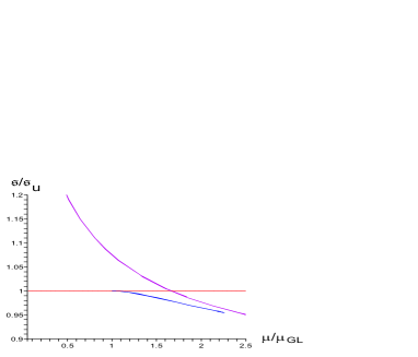
Figure 4: Entropy $\mathfrak{s}/\mathfrak{s}_{\rm u}$ versus the mass $\mu/\mu_{GL}$ diagram for the uniform string (red), non-uniform string (blue) and localized black hole (purple) branches.

The viewpoint that an unstable uniform string decays to a localized black hole has been challenged in [17]. In this work it is shown that in a classical evolution an event horizon cannot change topology, $i.e.$ it cannot pinch off in finite affine parameter (on the event horizon).

However, this does not exclude the possibility that a classically unstable horizon pinches off in infinite affine parameter [73]. Indeed, in [75, 76] the numerical study [74] of the classical decay of a uniform black string in five dimensions was reexamined, suggesting that the horizon of the string pinches off in infinite affine parameter.

Interestingly, the classical decay of the uniform string is quite different for $d\geq 13$. As we reviewed above, the results of [31] show that for $d\geq 13$ the non-uniform string has decreasing mass $\mu$ for decreasing $n$, as it emanates from the uniform string at the Gregory-Laflamme point at $\mu=\mu_{\rm GL}$. This means that the entropy of a non-uniform black string is higher than the entropy of a uniform string with same mass. Hence, for $d\geq 13$ we have a certain range of masses where the uniform black string is unstable, and where a non-uniform black string exists with higher entropy. This suggests that a uniform black string in that mass range will decay classically to a non-uniform black string. This type of decay can occur in a finite affine parameter, according to [17], since the horizon topology remains fixed during the decay.

Note that the range of masses for which we have a non-uniform string branch with higher entropy is extended by the fact that we have copies of the non-uniform string branch. The copies, which have the thermodynamic quantities given by the transformation rule (3.19), can easily be seen from the Intersection Rule of [47] (see Section 3.1) to have higher entropy than that of a uniform string of the same mass, since they also have decreasing $\mu$ for decreasing $n$. Thus, for $d\geq 13$, it is even possible that there exists a non-uniform black string for any given $\mu<\mu_{\rm GL}$ with higher entropy than that of the uniform black string with mass $\mu$. This will occur if the non-uniform string branch extends to masses lower than $2^{3-d}\mu_{\rm GL}$. Otherwise, the question of the endpoint of the decay of the uniform black string will involve a quite complicated pattern of ranges.

We will return to the $d$-dependence of the phase diagram in Section 4.1 where we consider the large $d$ behavior of a number of relevant quantities.

3.3 Phases with Kaluza-Klein bubbles

Until now all the solutions we have been discussing lie within the range $0\leq n\leq 1/(d-2)$. But, there are no direct physical restrictions on $n$ preventing it from being in the range $1/(d-2)<n\leq d-2$. Hence, the question arises about the existence of solutions in this range. This question was answered in [50] where it was shown that pure gravity solutions with Kaluza-Klein bubbles can realize all values of $n$ in the range $1/(d-2)<n\leq d-2$.

In this subsection we start by reviewing the place of the static Kaluza-Klein bubble (see Section 2.3) in the $(\mu,n)$ phase diagram. We then discuss the main properties of bubble-black hole sequences, which are phases of Kaluza-Klein black holes involving Kaluza-Klein bubbles. In particular, we comment on the thermodynamics of these solutions. Subsequently, we present the five- and six-dimensional phase diagrams as obtained by including the simplest bubble-black hole sequences. Finally, we comment on non-uniqueness in the phase diagram.

3.3.1 Static Kaluza-Klein bubble

In Section 2.3 we reviewed the static Kaluza-Klein bubble. Since it is a static solution of pure gravity that asymptotes to $\mathcal{M}^{d}\times S^{1}$ the static Kaluza-Klein bubble belongs to the class of solutions we are interested in. Thus, it is part of our phase diagram, and using (3.1), (3.2), (3.3), (3.5) and (2.31) we can read off $\mu$ and $n$ as

$$\mu=\mu_{\rm b}=\Omega_{d-2}\left(\frac{d-3}{4\pi}\right)^{d-3}\ ,\ \ n=d-2\ .$$ (3.20)

These expressions give the static Kaluza-Klein bubble as a specific point in the $(\mu,n)$ phase diagram. This is consistent with the fact that this solution does not have any free dimensionless parameters. Notice that $n=d-2$ precisely saturates the upper bound on $n$ in (3.4). In fact, a test particle at infinity will not experience any force from the bubble (in the Newtonian limit).

3.3.2 Bubble-black hole sequences

We now have a solution at $n=d-2$ with no event horizon, and hence no entropy or temperature. But so far in this review we have not mentioned any solutions lying in the range $1/(d-2)<n<d-2$. It was argued in [50] that such solutions exist and contain both Kaluza-Klein bubbles and black hole event horizons with various topologies.

For $d=4,5$ Emparan and Reall constructed in [112] exact solutions describing a black hole attached to a Kaluza-Klein bubble using a generalized Weyl ansatz, describing axisymmetric static space-times in higher-dimensional gravity. For $d=4$ this was generalized in [114] to two black holes plus one bubble or two bubbles plus one black string. There, it was also argued that the bubble balances the gravitational attraction between the two black holes, thus keeping the configuration in static equilibrium.

In [50] these solutions were generalized to a family of exact metrics for configurations with $p$ bubbles and $q=p,p\pm 1$ black holes in $D=5,6$ dimensions. These are regular and static solutions of the vacuum Einstein equations, describing alternating sequences of Kaluza-Klein bubbles and black holes, $e.g.$ for $(p,q)=(2,3)$ there is a sequence of the form:

$$\mathrm{black~{}hole}~{}-~{}\mathrm{bubble}~{}-~{}\mathrm{black~{}hole}~{}-~{}\mathrm{bubble}~{}-~{}\mathrm{black~{}hole}\,.$$

These solutions will be called bubble-black hole sequences and we will refer to particular elements in this class as $(p,q)$ solutions. This large class of solutions, which was anticipated in Ref. [112], includes the $(1,1)$, $(1,2)$ and $(2,1)$ solutions obtained and analyzed in [112, 114] as special cases.

We refer the reader to [50] for the explicit construction of these bubble-black hole sequences and a comprehensive analysis of their properties. Here we list a number of essential features:

• All values of $n$ in the range $1/(d-2)<n<d-2$ are realized.

• The mass $\mu$ can become arbitrarily large, and for $\mu\rightarrow\infty$ we have $n\rightarrow 1/(d-2)$.

• The solutions contain bubbles and black holes of various topologies. In the five-dimensional case we find black holes with spherical $S^{3}$ and ring $S^{2}\times S^{1}$ topology, depending on whether the black hole is at the end of the sequence or not. Similarly, in the six-dimensional case we find black holes with ring topology $S^{3}\times S^{1}$ and tuboid topology $S^{2}\times S^{1}\times S^{1}$, depending on whether the black hole is at the end of the sequence or not. The bubbles support the $S^{1}$’s of the horizons against gravitational collapse.

• The $(p,q)$ solutions are subject to constraints enforcing regularity, but this leaves $q$ independent dimensionless parameters allowing for instance the relative sizes of the black holes to vary. The existence of $q$ independent parameters in each $(p,q)$ solution is the reason for the large degree of non-uniqueness in the $(\mu,n)$ phase diagram, when considering bubble-black hole sequences.

Another interesting feature of the bubble-black hole sequences is that there exists a map between five- and six-dimensional solutions [50]. As a consequence there is a corresponding map between the physical parameters which reads

$$\mu^{(6D)}=\frac{2\pi}{3L^{(5D)}}\mu^{(5D)}\left(5-n^{(5D)}\right)\ ,\ \ n^{(6D)}=\frac{5n^{(5D)}-1}{5-n^{(5D)}}\ ,$$ (3.21)

$$\mathfrak{t}^{(6D)}_{k}=\mathfrak{t}^{(5D)}_{k}\ ,\ \ \mathfrak{s}^{(6D)}_{k}=\frac{4\pi}{L^{(5D)}}\mathfrak{s}^{(5D)}_{k}\ ,$$ (3.22)

where the superscripts $5D$ and $6D$ label the five- and six-dimensional quantities respectively. This form of the map assumes a certain normalization of the parameters of the solution, or equivalently, a choice of units, as further explained in Ref. [50].

3.3.3 Thermodynamics

For static space-times with more than one black hole horizon we can associate a temperature to each black hole by analytically continuing the solution to Euclidean space and performing the proper identifications needed to make the Euclidean solution regular near the locations of the Wick rotated event horizons. The temperatures of the black holes need not be equal, and one can derive a generalized Smarr formula that involves the temperature of each black hole. The Euclidean solution is regular everywhere only when all the temperatures are equal. It is always possible to choose the $q$ free parameters of the $(p,q)$ solution to give a one-parameter family of regular equal temperature solutions, which we denote $(p,q)_{\mathfrak{t}}$.

The equal temperature $(p,q)_{\mathfrak{t}}$ solutions are of special interest for two reasons. First, the two solutions, $(p,q)_{\mathfrak{t}}$ and $(q,p)_{\mathfrak{t}}$, are directly related by a double Wick rotation which effectively interchanges the time coordinate and the coordinate parameterizing the Kaluza-Klein circle. This provides a duality map under which bubbles and black holes are interchanged, giving rise to the following explicit map between the physical quantities of the solutions

$$\mu^{\prime}=n\mathfrak{t}^{d-3}\mu\ ,\ \ n^{\prime}=\frac{1}{n}\ ,\ \ \mathfrak{t}^{\prime}=\frac{1}{\mathfrak{t}}\ ,\ \ \mathfrak{s}^{\prime}=\frac{(d-2)n-1}{d-2-n}\mathfrak{t}^{d-1}\mathfrak{s}\ .$$ (3.23)

Secondly, for a given family of $(p,q)$ solutions, the equal temperature solution extremizes the entropy for fixed mass $\mu$ and fixed size of the Kaluza-Klein circle at infinity. For all explicit cases considered we find that the entropy is minimized for equal temperatures.

Furthermore, the entropy of the $(1,1)$ solution is always lower than the entropy of the uniform black string of the same mass $\mu$. We expect that all other bubble-black hole sequences $(p,q)$ have entropy lower than the $(1,1)$ solution, and this is confirmed for all explicitly studied examples. The physical reason behind the expectation that all bubble-black hole sequences have lower entropy than a uniform string of the same mass, is that some of the mass has gone into the bubble rather than the black holes, giving a smaller horizon area.

3.3.4 Phase diagrams for $d=4$ and $d=5$

The general $(\mu,n)$ phase diagrams for $d=4,5$ can in principle be drawn with all possible values $(p,q)$, though the explicit solution of the constraints becomes increasingly complicated for high $p,q$. However, the richness of the phase structure and the non-uniqueness in the $(\mu,n)$ phase diagram, is already illustrated by considering some particular examples of the general class of solutions, as was done in [50]. As an illustration, we give here the exact form of the curve for the (1,1) solution, corresponding to a bubble on a black hole,

$$d=4:\quad n_{(1,1)}(\mu)=\frac{1}{4}\left[-1+3\sqrt{1+\frac{8}{\mu^{2}}}\right]\qquad;\qquad d=5:\quad n_{(1,1)}(\mu)=\frac{1}{3}+\frac{4}{3\mu}\,.$$ (3.24)

in five and six dimensions respectively. These two solutions are related by the map in (3.21) and one may also check that these curves are correctly self-dual under the duality map (3.23).

In Figure 5 we have drawn for $d=4$ and $d=5$ the curves in the $(\mu,n)$ phase diagram for the $(p,q)=(1,1)$, $(1,2){}_{\mathfrak{t}}$ and $(2,1)$ solutions. These correspond to the configurations

$$\begin{array}[]{lccc}(1,1):&\mathrm{black~{}hole}&-&\mathrm{bubble}\\ D=5&S^{3}&&D\\ D=6&S^{3}\times S^{1}&&D\times S^{1}\end{array}$$ (3.25)

$$\begin{array}[]{lccccc}(1,2):&\mathrm{black~{}hole}&-&\mathrm{bubble}&-&\mathrm{black~{}hole}\\ D=5&S^{3}&&S^{1}\times I&&S^{3}\\ D=6&S^{3}\times S^{1}&&T^{2}\times I&&S^{3}\times S^{1}\end{array}$$ (3.26)

$$\begin{array}[]{lccccc}(2,1):&\mathrm{bubble}&-&\mathrm{black~{}ring}&-&\mathrm{bubble}\\ D=5&D&&S^{2}\times S^{1}&&D\\ D=6&D\times S^{1}&&S^{2}\times T^{2}&&D\times S^{1}\end{array}$$ (3.30)

where the first/second line in each configuration corresponds to the topology in five/six dimensions. Here $D$ denotes the disc and $I$ the line interval.

     

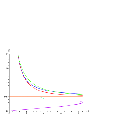
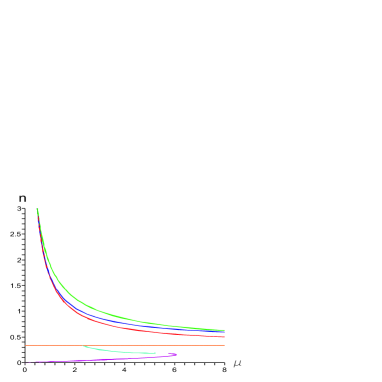
Figure 5: $(\mu,n)$ phase diagrams for five (left figure) and six (right figure) dimensions. We have drawn the $(p,q)=(1,1)$, $(1,2){}_{\mathfrak{t}}$ and $(2,1)$ solutions. These curves lie in the region $1/2<n\leq 2$ for the five-dimensional case and $1/3<n\leq 3$ for the six-dimensional case. The lowest (red) curve corresponds to the $(1,1)$ solution. The (blue) curve that has highest $n$ for high values of $\mu$ is the equal temperature $(1,2){}_{\mathfrak{t}}$ solution. The (green) curve that has highest $n$ for small values of $\mu$ is the $(2,1)$ solution. The entire phase space of the $(1,2)$ configuration is the wedge bounded by the equal temperature $(1,2){}_{\mathfrak{t}}$ curve and the $(1,1)$ curve. For completeness we have also included the uniform (orange) and non-uniform (cyan) black string branch, and the small black hole branch (magenta) displayed in Figure 3.

3.3.5 Non-uniqueness in the phase diagram

Finally we remark on the non-uniqueness of Kaluza-Klein black holes in the $(\mu,n)$ phase diagram. Clearly for a given mass there is a high degree of non-uniqueness. The non-uniqueness is not lifted by taking into account the relative tension $n$, as there are explicitly known cases of physically distinct solutions with the same mass and tension. For example the $(1,2){}_{\mathfrak{t}}$ solution and the $(2,1)$ solution intersect each other in the phase diagram. This means that we have two physically different solutions in the same point of the $(\mu,n)$ phase diagram. Moreover, there is in fact a continuously infinite non-uniqueness for certain points in the $(\mu,n)$ phase diagram. This is due to the fact that the $(p,q)$ solution has $q$ free parameters [50]. Hence, for given $p\geq 2$ and $q\geq 3$, we have $q-2$ free continuous parameters labeling physically different $(p,q)$ solutions, for certain points in the $(\mu,n)$ phase diagram.

4 More on the Gregory-Laflamme instability

In this section we present further results on the Gregory-Laflamme instability. First we discuss the large dimension limit of the GL critical mass and the phase diagram that emerges. The case of the GL instability for boosted neutral black strings, which has various interesting applications, will be discussed next. We also summarize some of the main results connecting the GL analysis to an LG (Landau-Ginzburg) analysis of the thermodynamics and what is known about the GL instability for neutral black branes with higher-dimensional compact spaces. Finally, we comment on an interesting connection between the GL instability and a classical membrane instability, known as the Rayleigh-Plateau instability.

4.1 Large $d$ limit

In Section 2.2 we reviewed the GL instability of the neutral black string in $d+1$ dimensions, and in particular presented the differential equations satisfied by the threshold mode. Unfortunately, no analytic solution to these equations is known and one has to solve them numerically for a given value of $d$ on a case by case basis. This was done for $d$ up to 50 in Ref. [31]. It is interesting to regard $d$ as a parameter in this system and study the behavior of the GL mode as $d$ becomes very large.

In Ref. [31] it was observed from the data that the critical mass exhibits the exponential behavior

$$\mu_{\rm GL}\simeq 16.21\cdot(0.686)^{d}$$ (4.1)

at large $d$. One can verify this result by solving analytically for the threshold mode in the large $d$ limit, as was done in Ref. [35]. Combined with the behavior of small localized black holes for large dimensions, this result enables us to conjecture the way the localized and non-uniform phases appear in the $(\mu,n)$ phase diagram when the dimension is large.

To derive the large $d$ behavior of the GL mode, it is convenient to start with the linear second order ODE that appears when considering the negative modes of a static and spherically symmetric perturbation of the Schwarzschild black hole in $d$ dimensions (see (2.29)). By taking the large $d$ limit, this ODE simplifies considerably and by dropping the exponentially growing solution, one finds

$$\chi(r)\sim{\cal K}_{\frac{d-1}{2}}(r)r^{-\frac{d-1}{2}}$$ (4.2)

where ${\cal K}_{s}$ is the modified Bessel function of the second kind (we remind the reader that the function $\chi(r)$ is related to the $h_{rr}$ component of the perturbation, $c.f.$ eqs. (2.11), (2.12)). The GL wave number $k_{\rm GL}\simeq\sqrt{d}$ can be determined by imposing the appropriate boundary conditions and the resulting GL mass takes the form [35]

$$\log\mu_{\rm GL}\simeq d\log\sqrt{\frac{e}{2\pi}}\ ,\ \ d\gg 1$$ (4.3)

This analytical result meshes very nicely with the earlier numerically obtained result (4.1).

Moreover, it is interesting to consider at large $d$ the slope of the localized black hole branch (3.17), measured in units normalized with respect to the Gregory-Laflamme point $(\mu_{\rm GL},n_{\rm GL}=1/(d-2))$, with $\mu_{\rm GL}$ given by the large $d$ formula (4.3). One finds

$$\frac{n}{n_{\rm GL}}\simeq d^{d/2}\frac{\mu}{\mu_{\rm GL}}\ ,\ \ d\gg 1~{}.$$ (4.4)

From this expression we see that the slope becomes infinitely steep as $d\rightarrow\infty$. This suggests that the curve describing the localized black hole and non-uniform black string branches should behave as sketched in Figure 6. In particular, the large $d$ behavior of the phase structure is expected to be such that the non-uniform string gets closer and closer to having $n=n_{\rm GL}=1/(d-2)$.

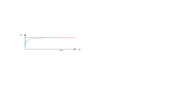
Figure 6: Sketch of the $(\mu,n)$ phase diagram for large $d$.

Further evidence for the above picture stems from the realization that the behavior (4.3) is equivalent to the critical Schwarzschild radius being equal to $r_{0}\simeq L/(2\pi)\sqrt{d}$. This shows that the large $d$ critical string is “fat”, and that most probably it cannot decay into a black hole since the black hole cannot fit into the compact dimension at the GL point [35]. Hence, the uniform black string should decay towards a different end-state, which presumably is the non-uniform black string.

Finally, from the comparison of the GL instability with the Jeans instability in Section 2.2 we recall that the Jeans instability predicts that the large $d$ behavior of the critical wave number is $k_{J}\sim d^{3/4}$. Now we see that this is different from the result $k_{c}\sim\sqrt{d}$ above. The classical Rayleigh-Plateau instability, on the other hand, does predict the correct large $d$ behavior as we will review in Section 4.4.

4.2 Boosted black strings

Another interesting direction that has been pursued in [116] is the study of the GL instability for boosted black strings. As we briefly review below it was found in [116] that the critical dimension (see Section 3.2) depends on the internal velocity and disappears for sufficiently large boosts. Moreover, the five-dimensional black ring [15] reduces in the large radius limit to a boosted neutral black string (in five dimensions), so these instabilities are also relevant to the stability analysis of black rings (we will briefly return to those issues in Section 8.1).

Boosted black strings can be obtained by boosting the static black string (2.9) along the $z$-direction. The resulting solution is

$$ds^{2} = -\left(1-\cosh^{2}\alpha\frac{r_{0}^{d-3}}{r^{d-3}}\right)dt^{2}+2\frac{r_{0}^{d-3}}{r^{d-3}}\cosh\alpha\sinh\alpha dtdz+\left(1+\sinh^{2}\alpha\frac{r_{0}^{d-3}}{r^{d-3}}\right)dz^{2}$$ (4.5)

$$+\left(1-\frac{r_{0}^{d-3}}{r^{d-3}}\right)^{-1}dr^{2}+r^{2}(d\theta^{2}+\sin^{2}\theta d\Omega_{d-3}^{2})~{}.$$

The mass and tension of the boosted black string can be computed from the general expressions (3.2), (3.3), (3.5), giving

$$\mu=\Omega_{d-2}\left(\frac{r_{0}}{L}\right)^{d-3}[(d-3)\cosh^{2}\alpha+1]\ ,\ \ n=\frac{(d-3)\sinh^{2}\alpha-1}{(d-3)\cosh^{2}\alpha+1}~{}.$$ (4.6)

In this case the string also carries the dimensionless momentum

$$p=\Omega_{d-2}(d-3)\cosh\alpha\sinh\alpha~{}.$$ (4.7)

One can now extend the original global thermodynamic argument of Gregory and Laflamme to this case, by comparing the entropy of the boosted black string (with horizon $r_{0}$ and boost $\alpha$) to the entropy of a boosted spherical black hole (with horizon $r_{0}^{\prime}$ and boost $\alpha^{\prime}$) with the same energy and momentum. Because we compare the solutions at the same energy and momentum, one can express $(r_{0}^{\prime},\alpha^{\prime})$ in terms of $(r_{0},\alpha)$ of the boosted black string. Then, equating the two entropies determines a minimal circumference [116]

$$L_{\rm min}=\frac{r_{0}}{\cosh\alpha}\frac{(d-1)^{d-1}}{[(d-3)(d-1)+\cosh^{-2}\alpha]^{(d-1)/2}}\frac{\Omega_{d-1}}{\Omega_{d-2}}$$ (4.8)

and hence from (4.6) one can define a maximum mass $\mu_{\rm max}\equiv\mu_{L=L_{\rm min}}$. This mass can be seen as a rough estimate of the point where the boosted black string becomes unstable. The instability appears for $\mu<\mu_{\rm max}$ (or $L>L_{\rm min}$). Note that $L_{\rm min}$ scales like $1/\cosh\alpha$, so this naive analysis suggests that the instability will persist for large boosts.

One can further analyze the instability of the boosted black string by appropriately boosting the time-dependent GL mode [116]. In this way, one finds that the instabilities of the boosted string can be related to instabilities of the static black string with complex frequencies. The relation is even more direct for the static threshold mode (2.15), on which one can simply apply the same boost that gave (4.5). As a result one finds the mode $\exp(i\omega t+ik_{c,{\rm boost}}z)$ with

$$k_{c,{\rm boost}}=\cosh\alpha k_{c}\ ,\ \ \omega=\sinh\alpha k_{c}$$ (4.9)

where $k_{c}$ is the threshold wave number for the static black string (see Table 1). So the threshold modes are waves that travel in the $z$-direction with the same speed as the boosted string. Note that the boost of the GL mode in a transverse direction, including the time-dependent one, was considered in Refs. [56, 66] and will be reviewed in Section 5.2.

Given the above results one can show that the critical dimension (see Section 3.2) depends on the boost parameter, and in fact disappears (for any given $d$) for large enough boost [116]. To see this observe from (4.9) that

$$L_{\rm GL,boost}=\frac{r_{0}}{\cosh\alpha}\left[\frac{(d-2)\Omega_{d-2}}{\mu_{GL}}\right]^{1/(d-3)}$$ (4.10)

and hence from (4.6),

$$\mu_{\rm GL,boost}=\frac{\cosh^{d-3}\alpha}{d-2}[(d-3)\cosh^{2}\alpha+1]\mu_{GL}$$ (4.11)

where $\mu_{GL}$ is the neutral GL mass. Comparing this to the $\mu_{\rm max}$ obtained above (see below (4.8)) one finds that for small boosts $\mu_{\rm max}>\mu_{\rm GL,boost}$ so that there is a regime where the boosted black string is stable, but the localized black hole has higher entropy, suggesting the existence of an unstable non-uniform black string in between. For zero boost this occurs for dimensions $D\leq 13$. On the other hand, for sufficiently large boosts one has $\mu_{\rm max}<\mu_{\rm GL,boost}$. So in this case, there is a regime, $\mu_{\rm max}<\mu<\mu_{\rm GL,boost}$, where the boosted black string is unstable but the localized black hole does not have a higher entropy, suggesting that the end-state is a stable non-uniform (boosted) black string in this range. In other words, for sufficiently large boosts the critical dimension disappears and we have a phase diagram that is analogous to that found for large $d$ in the neutral case in Fig. 6.

We will return to some other aspects of boosted black strings in Section 8.1

4.3 Higher-dimensional compact spaces

Most of the work on the stability and phases of black objects in spaces with compact transverse directions has been performed so far for the simplest case of one compact direction. Already for this case one observes a very rich phase structure. This phase structure is expected to become even richer as we go to higher dimensional compact spaces, such as $T^{n}$, $S^{n}$, $K3$ and $CY_{3}$ manifolds. As the number of moduli increases, the structure of the moduli space and hence the phase structure is clearly going to become more involved.

4.3.1 Instability of neutral black $p$-branes

The one higher-dimensional case that has been studied [35, 37] in more detail is that of the torus $\mathbb{T}^{p}$, which is the simplest generalization of the circle $S^{1}$. We summarize some of the main results here.

Consider neutral solutions of Einstein gravity with an event horizon, that asymptote to $\mathcal{M}^{d-1,1}\times\mathbb{T}^{p}$. Here we have the uniform black $p$-brane phase which is the obvious generalization of the black string, and is just a Schwarzschild-Tangherlini black hole in $d$ dimensions, with $p$ flat directions added $ds^{2}=\sum_{i=1}^{p}dz^{i}dz^{i}$ for the $p$-dimensional torus. The torus is defined by $p$ period vectors $\vec{e}_{i}$ such that any function $Y(\vec{z}+\vec{e})=Y(\vec{z})$ with $\vec{e}$ belonging to the integer lattice spanned by the period vectors. Performing a similar stability analysis as in Section 2.2, one finds that the threshold mode $P_{c,\mu\nu}(r)Y(\vec{z})$ satisfies [35]

$$\lambda_{\rm Sch}+\lambda_{\mathbb{T}^{p}}=0$$ (4.12)

where $\lambda_{\rm Sch}$ and $\lambda_{\mathbb{T}^{p}}$ are the eigenvalues in

$$\hat{\Delta}_{L}P_{c,\mu\nu}(r)=\lambda_{\rm Sch}P_{c,\mu\nu}(r)\ ,\ \ -\Delta Y(\vec{z})=\lambda_{\mathbb{T}^{p}}Y(\vec{z})$$ (4.13)

The only way to satisfy (4.12) is to take the GPY mode for the Schwarzschild black hole, and then it suffices to consider modes which are tensor on the Schwarzschild geometry and scalar on the torus. Consequently, we find that the instability of the black brane sets in when

$$r_{0}^{2}=\frac{k_{c}^{2}}{\lambda_{\rm min}}$$ (4.14)

where $k_{c}$ is the eigenvalue in (2.21) and $\lambda_{\rm min}$ is the mininimal (non-zero) eigenvalue of the Laplacian on the torus $\mathbb{T}^{p}$. In fact, this argument is general and applies to any stable compact manifold. For the case of $\mathbb{T}^{p}$ this eigenvalue is given explicitly by

$$\lambda_{{\rm min},\mathbb{T}^{p}}=|\vec{k}_{\rm min}|^{2}$$ (4.15)

where $\vec{k}_{\rm min}$ is the shortest vector in the reciprocal lattice of $\mathbb{T}^{p}$ ($i.e.$ the lattice spanned by the vectors $\vec{k}$ with $\vec{k}\cdot\vec{e}=2\pi n$, $n\in\mathbb{Z}$).

It is also physically clear that for a highly asymmetric torus, with $e.g.$ one large direction and the other ones small, the instability will set in for the mode along the large direction. In this sense the stability properties of black branes on such asymmetric tori are closely related to those of the black string. Hence, it seems more plausible that new effects will show up in the study of the other extreme, namely a square torus, with all directions of equal length. Moreover, understanding these two extremes may lead to a qualitative understanding of the intermediate region.

Recently, the Landau-Ginzburg method (see Section 4.4), was applied to the case of black $p$-branes on a square torus $\mathbb{T}^{p}$. In this case it is easy to see that $p$ modes (corresponding to each of the directions) become marginally tachyonic at the same GL point. Ref. [37] then studied the order of the phase transition, $i.e.$ the critical dimension, for such tori. It was shown that for the phase transition to be first order, it is enough to find a single direction in tachyon space for which this is the case. It was furthermore shown that in order to study the $\mathbb{T}^{p}$ case one needs to combine the known results for the $S^{1}$ case together with results for the $\mathbb{T}^{2}$. As a result it was concluded that the transition order for square tori depends only on the number of extended dimensions $d$, and not on $p$. In other words, the critical dimension discussed in Section 3.2 for $p=1$ is unchanged when considering higher-dimensional square tori. Note that in an earlier work [35] (see also [117]) a more naive analysis based on the comparison of the entropy of black holes localized in the compact directions and the entropy of black branes seemed to indicate that the critical dimension could become lower as the number of compact directions increases. As explained in [37], this conclusion is misleading because the corrections to the entropy of localized black holes can be shown to have an important effect in this case, and these were ignored in the analysis of [35]. More generally, this shows that one should be cautious when using the Schwarzschild black hole entropy as an approximation to make qualitative statements, $i.e.$ one should carefully study the effects of corrections due to the presence of the compact manifold.

4.3.2 Phase structure for higher tori

So far we have just considered the aspect of instability of uniform black branes with compact transverse directions, but if we think about possible phases it is not difficult to see that this will be very rich. Consider, for example, the case of the two-torus. First of all, for any phase of Kaluza-Klein black holes on $\mathcal{M}^{1,d-1}\times S^{1}$ we trivially get a phase for the case of $\mathcal{M}^{1,d-1}\times\mathbb{T}^{2}$ by adding a flat compact direction. This includes the uniform black two-brane phase discussed above, but also $e.g.$ semi-localized black holes of horizon topology $S^{d-1}\times S^{1}$ (these are of black string type) as well as bubble-black hole sequences with an extra circle direction. There are also going to be entirely new phases each time we add a compact direction. For example, in the case discussed above, there is also a phase of black holes that are localized in two of the $\mathbb{T}^{2}$-directions, $i.e.$ a phase with horizon topology $S^{d}$. These solutions reduce to the $(d+2)$-dimensional Schwarzschild black hole in the limit of zero mass, and it would be interesting to obtain the first order correction away from the zero mass limit using the methods of [38, 39] or [40]. There are also new bubble-black hole sequences for the case of $d=5,6$ (see for example the Conclusion of [50]) that are in principle not difficult to construct explicitly. All these will be part of some complicated higher dimensional phase structure with a complicated pattern of (in)stabilities.

4.3.3 Comments on general compact Ricci flat manifolds

More generally we may consider KK black hole solutions in $(d+p)$-dimensional pure gravity asymptoting to $\mathbb{R}^{d-1,1}\times{\cal N}_{p}$, with ${\cal N}_{p}$ being a generic $p$-dimensional compact Ricci flat manifold, for example a compact Calabi-Yau manifold. In this case, the phase diagram of neutral, static black hole solutions will be parameterized by the mass ${\cal M}$, the components of a generalized tension tensor ${\cal T}$ and the moduli that characterize the manifold ${\cal N}_{p}$ at infinity (minus one for the overall volume of ${\cal N}_{p}$ that can be scaled away). The components of the tension tensor ${\cal T}$ are straightforward generalizations of the single tension $n$ appearing above and can be thought of as the chemical potentials corresponding to the moduli of ${\cal N}_{p}$. See Ref. [104] for a treatment of the two-torus case, including a derivation of the first law of thermodynamics.

To obtain the uniform black membrane solution we simply tensor the $d$-dimensional Schwarzschild solution with the Ricci flat metric of ${\cal N}_{p}$

$$ds^{2}=-\left(1-\frac{r_{0}^{d-3}}{r^{d-3}}\right)dt^{2}+\left(1-\frac{r_{0}^{d-3}}{r^{d-3}}\right)^{-1}dr^{2}+r^{2}d\Omega^{2}_{d-2}+ds^{2}_{{\cal N}_{p}}~{}.$$ (4.16)

An obvious generalization of the argument appearing around eq. (4.12) suggests again the presence of a Gregory-Laflamme instability. The discussion of the higher tori case above indicates the presence of many more stable or unstable phases in the phase diagram with a complicated pattern of (in)stabilities. Beyond the phases of localized black holes, non-uniform black membranes and bubble-black hole sequences one can imagine new “uniform” phases, where the ${\cal N}_{p}$ moduli are radially varying, the tension tensor ${\cal T}^{ab}$ has values other than those of the uniform black brane solution (4.16) and the metric components have no dependence on the coordinates of ${\cal N}_{p}$. Black hole solutions of a similar spirit are abundant in extended supergravity, for example in $d=4$, ${\cal N}=2$ supergravity [118, 119] (see [120] for a recent review).

In general, many features of the phase diagram are expected to be strongly correlated with the topology of the compact manifold ${\cal N}_{p}$. It would be interesting to explore this connection further.

4.4 Other developments

We conclude this section by briefly discussing several other developments related to the GL instability and the Kaluza-Klein black hole phase diagram. These include an application of the Landau-Ginzburg theory of phase transitions, the use of Morse theory and the study of the merger point, where the black string and black hole branches meet. While these developments are important and very interesting, we choose to be brief here since many of these are very nicely explained in the review [27] by Kol. We also comment on a recent connection observed in Ref. [36] between the (classical) Rayleigh-Plateau instability of membranes and the GL instability.

4.4.1 LG in GL

Some of the features of the black hole-black string transition, in particular the order of the phase transition, can be nicely studied using the Landau-Ginzburg (LG) theory for the thermodynamics, as was done in Refs. [34, 27, 37] (see also [29, 30, 31]). We briefly summarize some of the main results here, referring the reader to the review [27] for a useful exposé of the general idea and further details, as well as the recent article [37] where a new method for determining the order of the phase transition was developed based on the LG perspective.

In statistical physics the Landau-Ginzburg theory [121] determines the order of a phase transition from the local behavior of the free energy $F$ near a critical point. For a simple system parameterized by a single variable $\lambda$ and a control parameter $\mu$ the free energy is a function $F=F(\lambda;\mu)$. We are interested in systems where a certain parity symmetry forces the free energy to be an even function of $\lambda$, $i.e.$ $F=F(\lambda^{2};\mu)$. For such systems the existence of a marginally tachyonic mode at some critical value $\mu_{c}$ of the control parameter implies that we can expand $F$ near $\lambda=0$, $\mu=\mu_{c}$ in a power series in $\lambda$

$$F=F_{1}(\mu-\mu_{c})\lambda^{2}+F_{2}\lambda^{4}+{\cal O}(\lambda^{6})~{},$$ (4.17)

where without loss of generality we can take the constant $F_{1}$ to be positive. The two possible behaviors of $F$ are summarized in Figures 7, 8 and are distinguished by the sign of the quartic coefficient $F_{2}$.

For negative $F_{2}$ (see Fig. 7) the system undergoes a first order transition. As $\mu$ is varied the system passes from a symmetric stable phase ($\lambda=0$ and $\mu>\mu_{c}$) to an unstable symmetric phase. Since $F$ is bounded from below there is a new stable asymmetric vacuum at finite $\lambda$ and the system discontinuously jumps to this new stable vacuum when $\mu<\mu_{c}$.

For positive $F_{2}$ (see Fig. 8) the system undergoes a second (or higher) order phase transition. As we vary $\mu$ from $\mu>\mu_{c}$ to $\mu<\mu_{c}$ the system passes continuously from the stable symmetric vacuum at $\lambda=0$ to a new asymmetric vacuum at $\lambda\neq 0$.

The non-uniform black string exhibits similar behavior with details that depend crucially on the space-time dimension. In the language of the above one-dimensional example, we can think of $\lambda$ as a parameter that measures how far the black string is from the uniform solution. This role can be played by the amplitude of the marginally tachyonic GL mode (2.21), $i.e.$ $\lambda$ can be taken as the coefficient of the threshold mode metric perturbation

$$h\sim\lambda~{}e^{ik_{c}z}~{}P_{c}~{}.$$ (4.18)

The control parameter $\mu$ can be taken as the mass of the black brane solution, or better yet in the canonical ensemble as the dimensionless ratio $\beta/L$ of the inverse temperature over the $z$ radius.

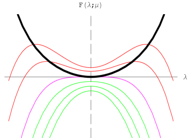
Figure 7: The typical behavior of the free energy during a first order phase transition. The red lines are at constant values of $\mu>\mu_{c}$ and the green lines at constant $\mu<\mu_{c}$. The thick black line represents a set of unstable asymmetric ($\lambda\neq 0$) vacua at $\mu>\mu_{c}$. The dashed horizontal line represents the symmetric $(\lambda=0)$ phase of the system, which is stable at $\mu>\mu_{c}$ and unstable at $\mu\leq\mu_{c}$.

When dealing with gravity one has to consider the free energy

$$-\beta F[g_{\mu\nu}]=I_{GH}[g_{\mu\nu}]=\frac{1}{16\pi G_{N}}\left(\int_{{\cal M}}R+2\int_{{\partial}{\cal M}}(K-K^{0})\right)~{},$$ (4.19)

as a function on the infinite dimensional configuration space of all metrics with given boundary conditions. For black branes smeared on a transverse $\mathbb{T}^{p}$ space the corresponding Landau-Ginzburg analysis around the uniform solution has been performed in [37]. In this system one finds a generalized multi-dimensional version of (4.17), which arises by analyzing the geometry of the non-uniform black brane up to second order in perturbation theory (for more details we refer the reader to [37]). The order of the transition is determined by the sign of an appropriate set of quartic coefficients in the free energy expansion. One finds that the result depends crucially on the dimension $d=D-p$ of the non-compact part of the space time (see also comments in Section 4.3). For $D\leq 12$ the transition is first order and the phase diagram looks like Fig. 3, whereas for $D\geq 13$ the transition is second order and the phase diagram becomes as in Fig. 6. Hence, there is an interesting critical dimension “$D^{*}=12.5$” where the behavior of the system changes dramatically.

The order of the phase transition for a black string on $\mathbb{R}^{3,1}\times S^{1}$ was first determined with a different method by Gubser in [29] and was improved upon by Wiseman in [30]. This computation was generalized to a more general background $\mathcal{M}^{d}\times S^{1}$ in [31] where the critical dimension $D^{*}$ was first observed. In addition, [122] pointed out that the critical dimension depends also on the ensemble; in the micro-canonical ensemble the critical dimension is one unit higher than that in the canonical ensemble.

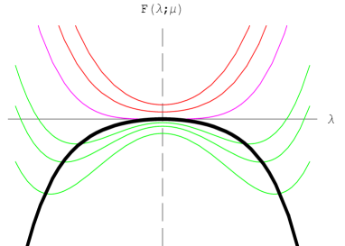
Figure 8: The typical behavior of the free energy during a second (or higher) order phase transition. Again, the red lines are at constant values of $\mu>\mu_{c}$ and the green lines at constant $\mu<\mu_{c}$. The thick black line represents a set of stable asymmetric ($\lambda\neq 0$) vacua at $\mu<\mu_{c}$. The dashed horizontal line represents the symmetric $(\lambda=0)$ phase of the system, which is stable at $\mu>\mu_{c}$ and unstable at $\mu\leq\mu_{c}$.

4.4.2 Morse theory

Another useful method that has been applied to address the issue of the endpoint of the decay of the unstable black string is Morse theory [123], as originally proposed in [34] and reviewed in [27]. While Landau-Ginzburg theory can be employed to study the local properties of the phase diagram, Morse theory can be used to obtain information about the global (topological) structure of the phase diagram.

In general, when we try to determine the pattern of static solutions in the phase diagram of Kaluza-Klein black holes on $\mathcal{M}^{d}\times S^{1}$, we are in essence studying the extrema of the gravitational action in the space of metrics with given boundary conditions. Morse theory can be useful in this study, since it is, by definition, the topological theory of the extrema of functions on a given manifold. For instance, it can be used to put constraints on how the extrema of a function behave under continuous deformations. The latter aspect of Morse theory was employed in [34] to argue that a natural completion of the black string phase diagram involves a point, called the ”merger point”, where the non-uniform black string branch meets the localized black hole branch.

The intuitive argument behind this analysis is based on the fact that we know that there is a localized black hole phase as well as a non-uniform black string phase, but a priori not where these phases end in the phase diagram. Since it is unphysical for a phase to end in nothing, it follows by “phase conservation” that the simplest possibility is that these two phases meet in a topology changing phase transition, the merger point.

4.4.3 Merger point

The prediction of a merger point in the phase diagram of black strings implies an intriguing topology changing transition where the black string horizon with topology $S^{d-2}\times S^{1}$ pinches off and becomes a black hole horizon with topology $S^{d-1}$. This transition reminds of the Gross-Witten transition [124] in two dimensional large $N$ gauge theories. Also certain features of the topology change near the merger point resemble the conifold transition in the moduli space of Calabi-Yau threefolds [125].

To this effect, it was argued in Ref [34] that not only does the horizon topology change, but also the local topology in the Euclidean section. This topology change can be modelled in analogy to the conifold transition as a pyramid, with the singular topology being the cone over $S^{d-2}\times S^{2}$,

$$ds^{2}=d\rho^{2}+\frac{\rho^{2}}{d-1}[d\Omega_{2}^{2}+(d-3)d\Omega_{d-2}^{2}]$$ (4.20)

which was termed the “double-cone”. Here, $\rho$ measures the distance from the tip of the cone and the constant prefactors ensure Ricci-flatness. Refs. [52, 33] show that the local geometry around the “waist” of the most nonuniform solutions is indeed cone-like to a good approximation.

Evidence for the merger point transition has been found with a numerical study in [52, 33]. Interesting parallels between the merger point transition and the Choptuik scaling in black hole formation [72] have been observed in [68, 69, 70, 71]. More details about the merger point can be found in the original work [34] and the review [27].

4.4.4 Rayleigh-Plateau instability

The first law of thermodynamics

$$dM={\cal{T}}dA~{},$$ (4.21)

$A$ being the horizon area, suggests a natural parallel between the mechanics of black holes and hydrodynamics. Indeed, by viewing (4.21) as a law for fluids where ${\cal{T}}$ is interpreted as an effective surface tension one is led to a simple picture of black holes, where the event horizon is treated as a kind of membrane with well-defined mechanical, electrical and magnetic properties [126]. It has been noticed that the membrane approach works surprisingly well in reproducing various aspects of black hole physics in different contexts (see for instance [127, 128] for an application in the context of AdS/CFT).

The membrane analogy was applied to black branes in [36, 129], where it was observed that there is an impressive correspondence between the Rayleigh-Plateau instability of long fluid cylinders and the Gregory-Laflamme instability of black strings [36]. Both instabilities are long-wavelength instabilities involving only the axisymmetric $s$-modes (for the black string this statement has been verified in [130]). The critical wave numbers $k_{RP}$ and $k_{c}$ agree exactly at large dimension $d$ - in particular they both scale as $\sqrt{d}$ for $d\gg 1$ - and there is qualitative agreement between the behavior of the instability time scales. Hence, this classical system appears to provide a better description of the Gregory-Laflamme instability as compared to the Jeans instability (see Section 2.2).

5 Instabilities in supergravity

Our discussion of the GL instability has so far been entirely within the context of Einstein gravity. A natural question is whether GL-like instabilities can also arise in the presence of matter fields, such as scalar fields and gauge potentials. This question is especially relevant in supergravity theories which appear in the low-energy limit of string theory. In this context one encounters a variety of black brane solutions whose stability properties are not only important in their own right, but can also have non-trivial consequences for their dual non-gravitational theories via the gauge/gravity correspondence (see Section 7).

Gregory and Laflamme already considered instabilities of charged branes in [3, 131]. Further work in this direction appeared in [132, 62, 63, 64, 65, 133, 134, 135, 136, 137, 138, 139, 55, 56, 57, 59, 60, 61, 140, 122, 67, 66, 141].

The investigation into the classical stability of charged branes began with the study of non-extremal singly-charged black $p$-branes [3, 131, 64, 135, 136, 138, 141]. In this case, there is a GL instability when the charge is sufficiently small compared to the total mass of the brane, whereas the brane is stable for large charge, $i.e.$ close to extremality. This has been shown using numerical methods. In Section 6 we comment on how this is related to the thermodynamics of these branes. In this review we consider instead the case of smeared non-extremal singly-charged black $p$-branes. The reason is that in this case we can be more precise, since we can explicitly find the GL instability by mapping it from the GL instability of the neutral black string [56, 66].

Before turning to the GL instability of non- and near-extremal smeared branes, we review the boost/U-duality map between phases of neutral Kaluza-Klein black holes and this class of branes [57] (see also [55, 56, 122]). This map suggests the presence of a GL instability in the case of non- and near-extremal smeared branes, which we then proceed to verify more explicitly. We also review recent work on GL instabilities of D-brane bound states that appeared in Refs. [59, 60, 61].

5.1 New phases of non- and near-extremal branes

The starting point of our discussion is the set of $1/2$ BPS branes in type IIA/B string theory and M-theory with a circle in the transverse space. We would like to consider the class of solutions that arise as thermal excitations of these branes. We will refer to the branes in this class as non-extremal branes on a circle. The near-extremal limit of these solutions will be defined in a way that keeps the non-trivial physics related to the presence of the circle. We will refer to this particular class of near-extremal branes as near-extremal branes on a circle. The dual non-gravitational theories living on these branes will be reviewed briefly in Section 7.

In analogy with the neutral Kaluza-Klein black holes of Section 3, one can define phase diagrams for the non- and near-extremal branes on a circle. See Ref. [57] for details and conventions. For non-extremal branes on a circle the dimensionless asymptotic quantities are the mass $\bar{\mu}$, the relative tension in the circle direction $\bar{n}$ and the charge $q$. For near-extremal branes on a circle there are two quantities, the energy above extremality $\epsilon$, rescaled to be dimensionless, and the relative tension $r$ which is the ratio between the tension of the brane along the transverse circle and the energy. The tension is measured using the general tension formula found in [97] that holds for non-asymptotically flat spaces. Hence, the resulting phases can be plotted in a two-dimensional $(\epsilon,r)$ phase diagram.

In this section we review the following:

• One can transform any static and neutral Kaluza-Klein black hole to a non-extremal brane on a circle with a combined boost and U-duality transformation. For a given charge $q$, this gives a map from points in the $(\mu,n)$ phase diagram to points in the non-extremal $(\bar{\mu},\bar{n})$ phase diagram.

• By taking a particular near-extremal limit of the map to non-extremal branes, one can transform any static and neutral Kaluza-Klein black hole to a near-extremal brane on a circle. In particular, this provides a map relating points in the $(\mu,n)$ phase diagram to points in the $(\epsilon,r)$ phase diagram.

• The above maps can be applied to the known phases of neutral Kaluza-Klein black holes, from which we generate (new) phases of non- and near-extremal branes on a circle.

5.1.1 Extremal $p$-branes

We consider here a class of branes that are thermal excitations of the $1/2$ BPS branes of type IIA and IIB string theory and M-theory. The singly-charged dilatonic $p$-branes in a $D$-dimensional space-time are solutions to the equations of motion of the action

$$I_{D}=\frac{1}{16\pi G_{D}}\int d^{D}x\sqrt{-g}\left(R-\frac{1}{2}\partial_{\mu}\phi\partial^{\mu}\phi-\frac{1}{2(p+2)!}e^{a\phi}(F_{(p+2)})^{2}\right)\ ,$$ (5.1)

where $\phi$ is the dilaton field and $F_{(p+2)}$ is a $(p+2)$-form field strength with $F_{(p+2)}=dA_{(p+1)}$ and $A_{(p+1)}$ the corresponding $(p+1)$-form gauge field. For $D=10$ the action (5.1) is the bosonic part of the low energy action of type IIA and IIB string theory (in the Einstein-frame) when only one of the gauge-fields is present. For $D=11$ it is the low energy action of M-theory for suitable choices of $a$ and $p$.

The extremal $1/2$ BPS $p$-brane solutions in string and M-theory take the well-known form

$$ds^{2}=H^{-\frac{d-2}{D-2}}\left[-dt^{2}+\sum_{i=1}^{p}(du^{i})^{2}+Hds_{d}^{2}\right]\ ,$$ (5.2)

$$e^{2\phi}=H^{a}\ ,\ \ A_{(p+1)}=(H^{-1}-1)dt\wedge du^{1}\wedge\cdots\wedge du^{p}\ ,$$ (5.3)

with $\nabla^{2}H=0$ (away from the sources). $ds_{d}^{2}$ denotes the metric and $\nabla^{2}$ the Laplacian of the $d$-dimensional transverse space. The solutions (5.2), (5.3) represent the $1/2$ BPS extremal $p$-branes of String/M-theory when $D=10,11$ and

$$a^{2}=4-2\frac{(p+1)(d-2)}{D-2}\ .$$ (5.4)

With (5.4) obeyed we get for $D=10$ the D-branes ($a=(3-p)/2$), NS5-brane ($a=1$) and the F-string ($a=-1$) of type IIA and IIB string theory, and for $D=11$ the M2-brane and M5-brane of M-theory ($a=0$). Note that the string theory solutions are written here in the Einstein frame.

In the following we place the extremal solutions (5.2)-(5.3) on a transverse space of the form $\mathbb{R}^{d-1}\times S^{1}$. The thermal excitations of these solutions corresponds to the non-extremal solutions that we find below.

5.1.2 Charging up solutions via U-duality

Consider a static and neutral Kaluza-Klein black hole solution (see Section 3), $i.e.$ a static vacuum solution of $(d+1)$-dimensional General Relativity with at least one event horizon that asymptotes to $\mathcal{M}^{d}\times S^{1}$. We can always write the metric of such a solution in the form

$$ds^{2}_{d+1}=-Udt^{2}+\frac{L^{2}}{(2\pi)^{2}}V_{ab}dx^{a}dx^{b}\ ,$$ (5.5)

where $a,b=1,...,d$ and $V_{ab}$ is a symmetric tensor. $U$ and $V_{ab}$ are functions of $x^{1},..,x^{d}$. In the asymptotic region $U\rightarrow 1$ and $L^{2}(2\pi)^{-2}V_{ab}dx^{a}dx^{b}$ describes the cylinder $\mathbb{R}^{d-1}\times S^{1}$. The factor $L^{2}/(2\pi)^{2}$, where $L$ is the circumference of the circle in $\mathcal{M}^{d}\times S^{1}$, has been included in (5.5) for later convenience.

By adding $p+1$ (where $p=9-d$) flat directions, this solution is trivially uplifted to a solution of eleven-dimensional (super)gravity. Denoting these directions by $z_{i}$ ($i=1\ldots p$) and $y$, we perform a Lorentz boost in the $y$ direction

$$\left(\begin{array}[]{c}\displaystyle t_{\rm new}\\ \displaystyle y_{\rm new}\end{array}\right)=\left(\begin{array}[]{cc}\cosh\alpha&\sinh\alpha\\ \sinh\alpha&\cosh\alpha\end{array}\right)\left(\begin{array}[]{c}\displaystyle t_{\rm old}\\ \displaystyle y_{\rm old}\end{array}\right)\ .$$ (5.6)

The resulting boosted metric has an isometry in the $y$-direction so we can make an S-duality to obtain a non-extremal D0-brane solution of type IIA string theory. For $d<9$ the D0-brane is uniformly smeared along an $\mathbb{R}^{9-d}$ space and has transverse space $\mathbb{R}^{d-1}\times S^{1}$. One can use further U-dualities to transform the solution into a D$p$-brane solution, an F-string solution or an NS5-brane solution of type IIA/B String theory, or to an M2-brane or M5-brane solution of M-theory, depending on what dimension $d$ we start with. In this way we obtain non-extremal singly-charged $p$-branes on a transverse circle in $D$ dimensions with $D=d+p+1$ (for String/M-theory we have $D=10$/$D=11$). The resulting non-extremal solution takes the form

$$ds^{2}=H^{-\frac{d-2}{D-2}}\left(-Udt^{2}+\sum_{i=1}^{p}(du^{i})^{2}+\frac{L^{2}}{(2\pi)^{2}}H\,V_{ab}dx^{a}dx^{b}\right)\ ,$$ (5.7)

$$H=1+\sinh^{2}\alpha\,(1-U)\ ,$$ (5.8)

$$e^{2\phi}=H^{a}\ ,\ \ A_{(p+1)}=\coth\alpha\,(H^{-1}-1)dt\wedge du^{1}\wedge\cdots\wedge du^{p}\ .$$ (5.9)

Notice that $U\rightarrow 0$ near a event horizon in the metric (5.5) for the neutral solution. This translates after the map into an event horizon in the non-extremal solution (5.7)-(5.9). Since the harmonic function (5.8) stays finite and non-zero for $U\rightarrow 0$, we deduce that the source of the electric potential $A_{(p+1)}$ in (5.9) is hidden behind the event horizon. Note also that if there is a number of event horizons defined by $U=0$, the chemical potential $\nu=-A_{tu^{1}\cdots u^{p}}|_{U=0}=\tanh\alpha$ is the same for each disconnected component of the event horizon. In the following we assume that we have at least one event horizon present.

Using the map from (5.5) to (5.7)-(5.9) a Kaluza-Klein black hole solution in $d+1$ dimensions can be mapped to a corresponding solution of supergravity describing non- or near-extremal $p$-branes on a circle. The dimensions $d$ and $p$ are related by the equation $D=d+p+1$ with $D=10$ for string theory and $D=11$ for M-theory.

The map from (5.5) to (5.7)-(5.9) is a development of an earlier result in [38]. In [38] it was pointed out that one can map any neutral solution into a corresponding non- and near-extremal solution in supergravity for the class of Kaluza-Klein black holes that fall into the $SO(d-1)$-symmetric ansatz (3.11) of Ref. [38]. While this observation was made at the level of the equations of motion, the combined boost and U-duality transformation reviewed above reveals the physical reason behind the existence of this map and moreover shows that it works for any static and neutral Kaluza-Klein black hole.

Here we present a summary of the map between physical quantities of the non-extremal branes and physical quantities of the neutral Kaluza-Klein black holes (we refer the reader to [57] for more details on the boost/U-duality map). In terms of the definitions of Ref. [57]

$$\bar{\mu}=q+\frac{(d+n)}{2(d-1)}\mu+\frac{b^{2}q}{1+\sqrt{1+b^{2}}}\ ,\ \ \bar{n}=n\ ,\ \ b\equiv\frac{d-2-n}{2(d-1)}\frac{\mu}{q}$$ (5.10)

where $(\mu,n)$ (see (3.5), (3.3)) are the dimensionless mass and relative tension of the neutral Kaluza-Klein black hole and $(\bar{\mu},\bar{n},q)$ the dimensionless mass, relative tension and dimensionless charge of the non-extremal brane. For the temperature and entropy one finds

$$\bar{\mathfrak{t}}=\frac{\mathfrak{t}}{\cosh\alpha}\ ,\ \ \bar{\mathfrak{s}}=\cosh\alpha\mathfrak{s}\ ,\ \ \ ,\ \ \cosh\alpha(\mu,n,q)\equiv\frac{1+b+\sqrt{1+b^{2}}}{2\sqrt{b(1+\sqrt{1+b^{2}})}}$$ (5.11)

where $(\mathfrak{t},\mathfrak{s})$ and ($\bar{\mathfrak{t}},\bar{\mathfrak{s}}$) are the temperature and entropy of the neutral Kaluza-Klein black hole and non-extremal brane respectively.

5.1.3 Phases of non-extremal branes

We can now apply the above boost/U-duality map to the known phases of Kaluza-Klein black holes reviewed in Section 3. We restrict ourselves here to the lower part of the phase diagram $n\leq 1/(d-2)$, $i.e.$ the uniform black string, the non-uniform black string and localized black holes. Recall at this point that all these phases have $SO(d-1)$ symmetry and have a metric that can be taken to be of the form of the ansatz (3.11). Hence the corresponding non-extremal solutions are of the form (5.7)-(5.9) with the ansatz (3.11) substituted. The phases obtained from the bubble-black hole sequences [50] will be considered elsewhere [143].

Applying the map to the uniform string branch we recover the known phase of non- and near-extremal branes smeared on a circle, which we call the uniform phase. For the sake of clarity we write the solution explicitly here

$$ds^{2}=H^{-\frac{d-2}{D-2}}\left(-fdt^{2}+\sum_{i=1}^{p}(du^{i})^{2}+H\frac{L^{2}}{(2\pi)^{2}}\left[\frac{1}{f}dR^{2}+dv^{2}+R^{2}d\Omega_{d-2}^{2}\right]\right)\ ,$$ (5.12)

$$e^{2\phi}=H^{a}\ ,\ \ A_{(p+1)}=\coth\alpha\,(H^{-1}-1)dt\wedge du^{1}\wedge\cdots\wedge du^{p}\ ,$$ (5.13)

$$f=1-\frac{R_{0}^{d-3}}{R^{d-3}}\ ,\ \ H=1+\sinh^{2}\alpha\frac{R_{0}^{d-3}}{R^{d-3}}\ .$$ (5.14)

In Section 5.2 we demonstrate that this solution suffers from a GL instability which we relate to the GL instability of the uniform black string. The thermodynamic quantities of the solution will be given in Section 6.2 when we discuss thermodynamic stability and the correlated stability conjecture.

A strong indication of a possible instability can be deduced already by applying the map to the non-uniform black string branch from which we generate a new phase of non-extremal $p$-branes on a circle with a connected but not translationally invariant horizon around the circle, $i.e.$ a horizon which is non-uniformly distributed along the circle. We denote this phase as the non-uniform phase.

Using the map (5.10) from the neutral case to the non-extremal case we see that this new branch emerges out of the uniform phase (with $\bar{n}=1/(d-2)$) at the critical mass

$$\bar{\mu}_{\rm c}=q+\frac{(d-1)}{2(d-2)}\mu_{\rm GL}+\frac{b_{c}^{2}}{1+\sqrt{1+b_{c}^{2}}}q\ ,\ \ b_{c}\equiv\frac{(d-3)\mu_{\rm GL}}{2(d-2)q}\ .$$ (5.15)

We can furthermore use the map (5.10) on Eq. (3.15). This gives

$$\bar{n}(\bar{\mu};q)=\frac{1}{d-2}-\bar{\gamma}(q)(\bar{\mu}-\bar{\mu}_{c})\ ,\ \ 0\leq\bar{\mu}-\bar{\mu}_{c}\ll 1\ ,$$ (5.16)

$$\bar{\gamma}(q)=\gamma\left[\frac{d-1}{2(d-2)}-\frac{\gamma\mu_{\rm GL}}{2(d-1)}+\frac{b_{c}}{\sqrt{1+b_{c}^{2}}}\frac{(d-1)(d-3)+(d-2)\gamma\mu_{\rm GL}}{2(d-1)(d-2)}\right]^{-1}\ .$$ (5.17)

with $\gamma$ given in Table 3. Eq. (5.16) captures the behavior of the non-uniform phase of non-extremal branes on a circle for masses slightly higher than $\bar{\mu}=\bar{\mu}_{c}$. Note that $\bar{\gamma}(q)\rightarrow\gamma$ for $q\rightarrow 0$, as expected. We see from (5.16) that the non-uniform phase starts at $(\bar{\mu},\bar{n})=(\bar{\mu}_{c},1/(d-2))$ and continues with increasing $\bar{\mu}$ and decreasing $\bar{n}$ with a slope given by $\bar{\gamma}(q)$. It is not difficult to show [57] from the above results that the uniform phase has higher entropy than the non-uniform phase for the same mass $\bar{\mu}$, just as in the neutral case.

For those dimensions $d$ where further numerical data are available on the neutral non-uniform branch, one can use the map to derive the corresponding data for the non-uniform phase of non-extremal branes. In this way one can obtain, for a given charge $q$, diagrams for any thermodynamic quantity one may wish to consider.

In Section 5.2 we show explicitly that $\bar{\mu}_{c}$ is a critical GL mass for the uniform phase of non-extremal branes on a circle. This is natural in view of the fact that the non-uniform phase implies the presence of a marginal mode at that mass.

Finally, the map can be applied to localized black holes on a circle to generate a phase of non-extremal $p$-branes that are localized on a circle. This phase will be called the localized phase. Ref. [57] gives the background to first order in $(\bar{\mu}-q)$, obtained from (5.7)-(5.9) and the neutral solution of Ref. [39]. For the relative tension we have in this case

$$\bar{n}(\bar{\mu};q)=\frac{2(d-1)}{d}\lambda_{d}(\bar{\mu}-q)+{\cal{O}}\Big{(}(\bar{\mu}-q)^{2}\Big{)}\ ,\ \ \lambda_{d}\equiv\frac{(d-2)\zeta(d-2)}{2(d-1)\Omega_{d-1}}$$ (5.18)

In the $(\bar{\mu},\bar{n})$ phase diagram, the localized phase starts at the extremal point $(q,0)$ and goes upwards with a slope that can be read off from (5.18). The corresponding entropy and temperature of the branch can also be computed from the neutral thermodynamics. Again, for those dimensions $d$ where numerical data are available for the neutral phase, one can use the map to obtain corresponding diagrams for any thermodynamic quantity of the non-extremal localized phase.

5.1.4 Phases of near-extremal branes

Given the boost/U-duality map from neutral and static Kaluza-Klein black holes to non-extremal branes on a circle, we can go one step further and take the near-extremal limit. In this way, we obtain a map that takes a Kaluza-Klein black hole solution to a near-extremal brane solution on a circle.

The definition of the near-extremal limit of a non-extremal $p$-brane on a circle is

$$q\rightarrow\infty\ ,\ \ L\rightarrow 0\ ,\ \ g\equiv\frac{16\pi G_{D}}{V_{p}L^{d-2}}\ \,\mbox{fixed }\ ,\ \ l\equiv L\sqrt{q}\ \,\mbox{fixed }\ ,\ \ x^{a}\ \,\mbox{fixed }\$$ (5.19)

where $V_{p}$ is the (spatial) volume of the $p$-brane, $L$ the circumference of the circle, $q$ the rescaled charge and $x^{a}$ the transverse directions parameterizing $\mathbb{R}^{d-1}\times S^{1}$ in the asymptotic region. This definition ensures that the energy above extremality $\bar{\mu}-q$ is finite and sensitive to the non-trivial physics associated to the compact direction.

The near-extremal branes defined in this way can be characterized by two dimensionless quantities $(\epsilon,r)$ which are respectively rescaled versions of the energy above extremality and the tension in the circle direction (see [57] for the precise definitions). Applying the limit (5.19) to the general solution (5.12)-(5.14) we obtain the following result for near-extremal branes on a circle

$$ds^{2}=\hat{H}^{-\frac{d-2}{D-2}}\left(-Udt^{2}+\sum_{i=1}^{p}(du^{i})^{2}+\hat{H}V_{ab}dx^{a}dx^{b}\right)\ ,$$ (5.20)

$$e^{2\phi}=\hat{H}^{a}\ ,\ \ A_{(p+1)}=\hat{H}^{-1}dt\wedge du^{1}\wedge\cdots\wedge du^{p}\ ,$$ (5.21)

where

$$\hat{H}=\hat{h}_{d}\frac{1-U}{\hat{c}_{t}}\ ,\ \ \hat{h}_{d}\equiv\frac{l^{2}(2\pi)^{d-5}}{(d-3)\Omega_{d-2}}\ .$$ (5.22)

The fields in (5.20)-(5.21) have been written in units of $L/(2\pi)$, $i.e.$ we have rescaled the fields with the appropriate powers of $L/(2\pi)$ to get a finite solution. As a trivial check, one can show that the near-extremal $p$-brane solutions generated in this way correctly asymptote to the near-horizon limit of the extremal $p$-brane on a transverse circle (5.2), (5.3), which is taken as the reference space when calculating energy and tensions.

To summarize, we have seen that there is a direct map from any Kaluza-Klein black hole in $d+1$ dimensions to a near-extremal $p$-brane on a circle ($D=d+p+1$). The corresponding map between thermodynamic quantities gives the near-extremal quantities [57]

$$\epsilon=\frac{d+n}{2(d-1)}\mu\ ,\ \ r=2\frac{(d-1)n}{d+n}\ ,\ \ \hat{\mathfrak{t}}=\mathfrak{t}\sqrt{\mathfrak{t}\mathfrak{s}}\ ,\ \ \hat{\mathfrak{s}}=\frac{\mathfrak{s}}{\sqrt{\mathfrak{t}\mathfrak{s}}}\ ,$$ (5.23)

where $(\mu,n,\mathfrak{t},\mathfrak{s})$ and $(\epsilon,r,\hat{\mathfrak{t}},\hat{\mathfrak{s}})$ are the (rescaled) mass/energy, relative tension, temperature, entropy of the neutral Kaluza-Klein black hole and near-extremal brane respectively. The latter quantities are defined as

$$\epsilon=gE\ ,\ \ r=\frac{2\pi\hat{\mathcal{T}}}{E}\ ,\ \ \hat{\mathfrak{t}}=l\,\hat{T}\ ,\ \ \hat{\mathfrak{s}}=\frac{g}{l}\hat{S}$$ (5.24)

where $E$, ${\hat{\mathcal{T}}}$, $\hat{T}$, $\hat{S}$ are the energy, transverse tension, temperature, entropy of the near-extremal brane, and $l$ and $g$ appear in (5.19). With the use of (5.23) we can obtain the near-extremal $(\epsilon,r)$ phase diagram from the $(\mu,n)$ phase diagram of neutral Kaluza-Klein black holes.

In the above language the near-extremal Smarr formula and first law of thermodynamics take the form

$$\hat{\mathfrak{t}}\hat{\mathfrak{s}}=2\frac{d-2-r}{d}\epsilon\ ,\ \ \delta\epsilon=\hat{\mathfrak{t}}\,\delta\hat{\mathfrak{s}}$$ (5.25)

As a consequence, knowing a curve $r(\epsilon)$ in the near-extremal phase diagram determines the entire thermodynamics.

We can apply the above map to all the known phases of Kaluza-Klein black holes as we did with the non-extremal branes on a circle . Here we restrict ourselves again to the uniform, non-uniform and localized phase. Note that since these solutions fall within the ansatz (5.5), we know that the corresponding near-extremal branes will be of the form (5.20)-(5.22) with the ansatz substituted. Hence we get the following three phases of near-extremal branes on a circle:

• The uniform phase. In this phase a near-extremal brane is uniformly smeared on a transverse circle. The solution can be obtained with the map from the uniform black string and takes the well-known form

  $$ds^{2}=\hat{H}^{-\frac{d-2}{D-2}}\left(-fdt^{2}+\sum_{i=1}^{p}(du^{i})^{2}+\hat{H}\left[\frac{1}{f}dR^{2}+dv^{2}+R^{2}d\Omega_{d-2}^{2}\right]\right)\ ,$$ (5.26)

  $$e^{2\phi}=\hat{H}^{a}\ ,\ \ A_{(p+1)}=\hat{H}^{-1}dt\wedge du^{1}\wedge\cdots\wedge du^{p}\ ,$$ (5.27)

  $$f=1-\frac{R_{0}^{d-3}}{R^{d-3}}\ ,\ \ \hat{H}=\frac{\hat{h}_{d}}{R^{d-3}}\ ,\ \ \hat{h}_{d}\equiv\frac{l^{2}(2\pi)^{d-5}}{(d-3)\Omega_{d-2}}\ .$$ (5.28)

  Setting $n=1/(d-2)$ in (5.23) we find the relative tension $r=2/(d-1)$. The thermodynamics of the uniform phase is

  $$\hat{\mathfrak{s}}_{u}(\epsilon)=\frac{4\pi}{\sqrt{d-3}}(\Omega_{d-2})^{-\frac{1}{d-3}}\left(\frac{2\,\epsilon}{d-1}\right)^{\frac{d-1}{2(d-3)}}\ ,$$ (5.29)

  $$\hat{\mathfrak{f}}_{u}(\hat{\mathfrak{t}})=-\frac{d-5}{2}(\Omega_{d-2})^{-\frac{2}{d-5}}\left(\frac{4\pi\,\hat{\mathfrak{t}}}{(d-3)^{3/2}}\right)^{\frac{2(d-3)}{d-5}}\ .$$ (5.30)

  In Section 5.2 we demonstrate that the uniformly smeared near-extremal $p$-brane solution has a GL-instability.

• The non-uniform phase. This is a phase with a configuration of near-extremal branes that are non-uniformly distributed around a circle. This phase is obtained by applying the above near-extremal map to the non-uniform black string branch reviewed in Section 3. It emerges from the uniform phase given above at the critical energy

  $$\epsilon_{c}=\frac{d-1}{2(d-2)}\mu_{\rm GL}$$ (5.31)

  which follows from the map (5.23). The thermodynamics of this phase near the critical point is

  $$\frac{\hat{\mathfrak{s}}(\epsilon)}{\hat{\mathfrak{s}}_{u}(\epsilon)}=1-\frac{(d-1)^{2}}{4d(d-3)^{2}}\frac{\hat{\gamma}}{\epsilon_{c}}(\epsilon-\epsilon_{c})^{2}+\mathcal{O}((\epsilon-\epsilon_{c})^{3})\ .$$ (5.32)

  $$\hat{\mathfrak{f}}(\hat{\mathfrak{t}})=-\frac{d-5}{d-1}\epsilon_{c}-\hat{\mathfrak{s}}_{c}(\hat{\mathfrak{t}}-\hat{\mathfrak{t}}_{c})-\frac{c}{2\hat{\mathfrak{t}}_{c}}(\hat{\mathfrak{t}}-\hat{\mathfrak{t}}_{c})^{2}+\mathcal{O}((\hat{\mathfrak{t}}-\hat{\mathfrak{t}}_{c})^{3})\ ,$$ (5.33)

  with $\epsilon_{c}$ the critical energy (5.31), $\hat{\mathfrak{t}}_{c}$ and $\hat{\mathfrak{s}}_{c}$ the corresponding critical temperature and entropy, and $c$ the (rescaled) specific heat

  $$c=\frac{d(d-1)\hat{\mathfrak{s}}_{c}}{d(d-5)+2(d-1)\hat{\gamma}\epsilon_{c}}\ ,$$ (5.34)

  The numerical values $\epsilon_{c}$, $\hat{\gamma}$, $\hat{\mathfrak{t}}_{c}$, $\hat{\mathfrak{s}}_{c}$ and $c$, of the energy, slope, temperature, entropy and specific heat at the critical point are listed in Table 4 [57].

  $d$	$4$	$5$	$6$	$7$	$8$	$9$
  $\epsilon_{c}$	$2.64$	$1.54$	$1.09$	$0.71$	$0.46$	$0.31$
  $\hat{\gamma}$	$0.25$	$0.39$	$0.55$	$0.88$	$1.42$	$2.33$
  $\hat{\mathfrak{t}}_{c}$	$0.75$	$1$	$1.07$	$1.05$	$0.97$	$0.89$
  $\hat{\mathfrak{s}}_{c}$	$2.33$	$1.54$	$1.22$	$0.91$	$0.68$	$0.53$
  $c$	$-433$	$6.46$	$3.06$	$1.77$	$1.14$	$0.79$

  Table 4: In this table we list the critical energy $\epsilon_{c}$ and the constant $\hat{\gamma}$ determining the non-uniform phase of near-extremal branes on a circle for $0\leq\epsilon-\epsilon_{c}\ll 1$. In addition we list the critical temperature $\hat{\mathfrak{t}}_{c}$ and the critical entropy $\hat{\mathfrak{s}}_{c}$, as well as the heat capacity $c$ of the non-uniform phase at the critical point. These numbers are obtained in Ref. [57].

• The localized phase. This is a phase of a near-extremal brane localized on a transverse circle. It is obtained by applying the map to the black hole on cylinder branch. Since the black hole on cylinder branch starts at $(\mu,n)=(0,0)$, we deduce from the map (5.23) that the localized phase starts at $(\epsilon,r)=(0,0)$. The vanishing of the tension along the transverse circle is expected since the brane becomes completely localized on the circle in the limit $\epsilon\rightarrow 0$. Furthermore we can use the analytical results of Ref. [39] to explicitly compute the first correction to the solution and thermodynamics of the non- and near-extremal branes localized on a circle (see [57] for more details). The corresponding small black hole thermodynamics is

  $$\hat{\mathfrak{s}}(\epsilon)=\hat{C}_{1}^{(d)}\epsilon^{\frac{d}{2(d-2)}}\left(1+\frac{(d-1)\zeta(d-2)}{d(d-2)\Omega_{d-1}}\epsilon+{\cal{O}}(\epsilon^{2})\right)\ ,$$ (5.35)

  $$\hat{C}_{1}^{(d)}\equiv\frac{4\pi(\Omega_{d-1})^{-\frac{1}{d-2}}}{\sqrt{d-2}}\left(\frac{2}{d}\right)^{\frac{d}{2(d-2)}}$$ (5.36)

  and

  $$\hat{\mathfrak{f}}(\hat{\mathfrak{t}})=-\hat{K}_{1}^{(d)}\hat{\mathfrak{t}}^{\frac{2(d-2)}{d-4}}\left(1+\frac{2(d-1)\zeta(d-2)\hat{K}_{1}^{(d)}}{(d-4)^{2}\Omega_{d-1}}\hat{\mathfrak{t}}^{\frac{2(d-2)}{d-4}}+{\cal{O}}\Big{(}(\hat{\mathfrak{t}}^{\frac{2(d-2)}{d-4}})^{2}\Big{)}\right)\ ,$$ (5.37)

  $$\hat{K}_{1}^{(d)}\equiv\frac{d-4}{2}(\Omega_{d-1})^{-\frac{2}{d-4}}\left(\frac{4\pi}{(d-2)^{3/2}}\right)^{\frac{2(d-2)}{d-4}}\ .$$ (5.38)

  One may also compute the second order corrections to these expressions using the second order correction in (3.17). We leave this as an exercise for the reader.

From the analysis of the non-uniform phase we observe that, in parallel with the non-extremal case, we also have a map of the Gregory-Laflamme mass $\mu_{\rm GL}$ of the uniform black string branch to a critical energy $\epsilon_{c}$. This is the energy where the non-uniform phase connects to the uniform phase of near-extremal branes on a circle. The existence of the non-uniform phase suggests that near-extremal branes smeared on a circle have a critical energy below which they are classically unstable. This is indeed the case, as we show in Section 5.2.2.

5.2 GL-instability of smeared non- and near-extremal branes

In the previous subsection we reviewed the boost/U-duality transformation that takes a neutral black string to a D$p$-brane smeared on a transverse direction. Following Ref. [66] we describe in this subsection how to use this transformation to map the unstable GL mode of the neutral black string to the unstable mode of the non-extremal and near-extremal smeared D$p$-branes. As we take the extremal limit the unstable GL mode connects smoothly to the marginal modes of the extremal smeared brane.

5.2.1 Non-extremal smeared D$p$-branes

The boost/U-duality transformation of the previous subsection converts the uniform neutral black string solution (2.9) to the smeared D$p$-brane solution

$$ds^{2}=H^{-1/2}\left[-fdt^{2}+\sum_{i=1}^{p}dx_{i}^{2}\right]+H^{1/2}\left[f^{-1}dr^{2}+dz^{2}+r^{2}d\Omega^{2}_{7-p}\right]~{},$$ (5.39)

$$e^{2\phi} = H^{(3-p)/2}~{},~{}A_{01\cdots p}=\coth\alpha(H^{-1}-1)~{},~{}~{}f=1-\frac{r_{0}^{6-p}}{r^{6-p}}~{},~{}~{}H=1+\sinh^{2}\alpha(1-f)~{}.$$

This is the same solution as (5.12)-(5.14) now written in the string frame without the $\frac{L}{2\pi}$ rescaling $i.e.$ with dimensionful radial coordinate $r$ and $S^{1}$ coordinate $z\sim z+L$. Applying the transformation to the neutral GL mode (2.11), (2.12) will give (before the type II reduction) an eleven dimensional background with a non-normalizable exponential dependence on the M-theory circle direction $y$ (the critical case $k=k_{c}$ is an exception). It was pointed out in [56] that this problem can be avoided by considering a complex metric perturbation and finding a complex transformation that $i)$ gets rid of the exponential $y$ dependence and $ii)$ still has the same effect on the zeroth order part of the metric, $i.e.$ on the neutral black string metric. In the end one is instructed to take the real part of the transformed perturbation. This last step is allowed because the perturbed Einstein equations of motion are linear.

The precise form of the transformation is as follows. First define the coordinates $y^{\prime}$ and $\tilde{z}$ by making a complex rotation of the $y$ and $z$ coordinates

$$\left(\begin{array}[]{c}\displaystyle y^{\prime}\\ \displaystyle\tilde{z}\end{array}\right)=M\left(\begin{array}[]{c}\displaystyle y\\ \displaystyle z\end{array}\right)\ ,\ \ M=\left(\begin{array}[]{cc}\cosh w&-i\sinh w\\ i\sinh w&\cosh w\end{array}\right)\ .$$ (5.40)

Recall that the $y$ and $z$ directions correspond to the M-theory circle and transverse circle respectively. Notice that the neutral black string metric (2.9) embedded in eleven dimensional gravity is invariant under (5.40) since $(dy^{\prime})^{2}+(d\tilde{z})^{2}=dy^{2}+dz^{2}$. At the next step we supplement the transformation (5.40) with a boost that takes the $(t,y^{\prime})$ coordinates to the $(\tilde{t},\tilde{y})$ coordinates given by

$$\left(\begin{array}[]{c}\displaystyle\tilde{t}\\ \displaystyle\tilde{y}\end{array}\right)=\Lambda\left(\begin{array}[]{c}\displaystyle t\\ \displaystyle y^{\prime}\end{array}\right)\ ,\ \ \Lambda=\left(\begin{array}[]{cc}\cosh\alpha&\sinh\alpha\\ \sinh\alpha&\cosh\alpha\end{array}\right)~{}.$$ (5.41)

We choose the rotation parameters so that

$$\sinh w=\frac{\Omega}{k}\tanh\alpha\ ,\ \ \tilde{k}=k\cosh w\ ,\ \ \tilde{\Omega}=\frac{\Omega}{\cosh\alpha}~{}.$$ (5.42)

Then we can write the real part of the boosted perturbation of the eleven dimensional metric (obtained as described around (5.6)) as

$$\tilde{h}_{\mu\nu}=\mbox{Re}\left\{\exp\left(\frac{\tilde{\Omega}t}{r_{0}}+i\frac{\tilde{k}z}{r_{0}}\right)\tilde{P}_{\mu\nu}\right\}~{}.$$ (5.43)

Using the relation $\tilde{P}=\Lambda^{-1}M^{-1}P(M^{-1})^{T}(\Lambda^{-1})^{T}$ with $P$ given in (2.12) we find

$$\begin{array}[]{c}\displaystyle\tilde{P}_{tt}=-f\psi\cosh^{2}\alpha\ ,\ \ \tilde{P}_{yy}=-f\psi\sinh^{2}\alpha\ ,\ \ \tilde{P}_{ty}=f\psi\sinh\alpha\cosh\alpha\ ,\\[8.53581pt] \displaystyle\tilde{P}_{tr}=\eta\cosh\alpha\ ,\ \ \tilde{P}_{yr}=-\eta\sinh\alpha\ ,\ \ \tilde{P}_{rr}=f^{-1}\chi\ ,\ \ \tilde{P}_{\rm sphere}=r^{2}\kappa~{},\end{array}$$ (5.44)

where we made the relabelings $\tilde{t}\rightarrow t$ and $\tilde{y}\rightarrow y$. Notice that the complex rotation (5.40) precisely ensures that the exponential factor does not have a $y$-dependence. We can therefore apply the same U-duality transformations on (5.43)-(5.44) as on the boosted neutral black string. After these U-duality transformations, consisting of one S-duality and $p$ T-dualities, we conclude that the perturbed non-extremal D$p$-brane smeared on a transverse direction can be written as [66]

$$\begin{array}[]{c}\displaystyle\begin{array}[]{rcl}ds^{2}&=&\displaystyle H_{\rm c}^{-1/2}\left[-f_{\rm c}dt^{2}+\sum_{i=1}^{p}dx_{i}^{2}+2\eta\cosh\alpha{\cal E}dtdr\right]\\[14.22636pt] &&\displaystyle+H_{\rm c}^{1/2}\Big{[}f^{-1}(1+\chi{\cal E})dr^{2}+dz^{2}+r^{2}(1+\kappa{\cal E})d\Omega_{7-p}^{2}\Big{]}\ ,\end{array}\\[34.1433pt] \displaystyle e^{2\phi}=H_{\rm c}^{(3-p)/2}\ ,\ \ A_{01\cdots p}=\coth\alpha(H_{\rm c}^{-1}-1)\ ,\ \ A_{r1\cdots p}=-H^{-1}\eta\sinh\alpha{\cal E}\ ,\\[8.53581pt] \displaystyle f=1-\frac{r_{0}^{6-p}}{r^{6-p}}\ ,\ \ H=1+\sinh^{2}\alpha(1-f)\ ,\ \ f_{\rm c}\equiv f(1+\psi{\cal E})\ ,\ \ H_{\rm c}\equiv 1+\sinh^{2}\alpha(1-f_{\rm c})\ ,\\[8.53581pt] \displaystyle{\cal E}=\cos\left(\tilde{k}r_{0}^{-1}z\right)\exp\left(\tilde{\Omega}r_{0}^{-1}t\right)\ .\end{array}$$ (5.45)

The perturbed D$p$-brane background appears here in one compact expression. From this one can easily deduce the explicit form of the perturbation by expanding to first order. The unstable mode appearing in [56] is equivalent to (5.45) for $p=0$, though written in a different gauge.

Note that the functions $\psi$, $\eta$, $\chi$ and $\kappa$ are still solutions to Eqs. (A.7)-(A.15) with $f$ given by (A.2). In particular $\psi$ is a solution of Eq. (2.13). All these functions depend on the variable $x=rk/r_{0}$ just as in the case of the neutral black string perturbation.

Furthermore, we see from (5.42) that $\tilde{k}^{2}=k^{2}+\Omega^{2}\tanh^{2}\alpha$ and $\tilde{\Omega}=\Omega/\cosh\alpha$. Hence, we can obtain $\tilde{\Omega}$ as a function of $\tilde{k}$ by using the functional dependence $\Omega(k)$ for the neutral black string (as sketched for $p=0,...,5$ in Figure 1, where $p=9-d$). We note that the critical point $(k,\Omega)=(k_{c},0)$ is mapped to the critical point $(\tilde{k},\tilde{\Omega})=(k_{c},0)$, which corresponds to the marginal mode of the D$p$-brane with a transverse direction. This marginal mode appears at the origin of the non-uniform phase of non-extremal D$p$-branes with a transverse direction [57]. From Figure 1 we also deduce that $\tilde{k}<k_{c}$ for any $k<k_{c}$ and the function $\tilde{\Omega}(\tilde{k})$ never exhibits time-dependent modes with wavelength smaller than the critical one.

5.2.2 Near-extremal smeared D$p$-branes

It is straightforward to take the near-extremal limit (5.19) of the perturbed non-extremal solution (5.45). In order to make the connection with gauge theory quantities more transparent later on we find it convenient to define here the ’t Hooft and Yang-Mills couplings as

$$\lambda=g^{2}_{\rm YM}N~{},~{}~{}g^{2}_{\rm YM}=(2\pi)^{p-1}\hat{g}_{s}l_{s}^{p-2}~{},$$ (5.46)

where $\hat{g}_{s}$ is the T-dual string coupling. It can be expressed in terms of the circumference $\hat{L}$ of the T-dual circle (on which the D$(p+1)$-brane is wrapped) with the use of the T-duality relations

$$L\hat{L}=(2\pi l_{s})^{2}~{},~{}~{}g_{s}=\hat{g}_{s}\frac{2\pi l_{s}}{\hat{L}}~{}.$$ (5.47)

In these parameters it is convenient to re-express the near-extremal limit (5.19) as

$$l_{s}\rightarrow 0\ ,\ \ u=\frac{r}{l_{s}^{2}}\ ,\ \ \hat{z}=\frac{z}{l_{s}^{2}}\ ,\ \ g_{\rm YM}\ ,\ \ \hat{L}~{}~{}\mbox{fixed}\ .$$ (5.48)

Respectively, the uniform near-extremal smeared D$p$-brane solutions take the form

$$\begin{array}[]{c}\displaystyle l_{s}^{-2}ds^{2}=\hat{H}^{-1/2}(-fdt^{2}+\sum_{i=1}^{p}dx_{i}^{2})+\hat{H}^{1/2}(f^{-1}du^{2}+d\hat{z}^{2}+u^{2}d\Omega_{7-p}^{2})\ ,\\[8.53581pt] \displaystyle e^{2\phi}=\hat{H}^{\frac{3-p}{2}}\ ,\ \ A_{01\ldots p}=\hat{H}^{-1}\ ,\ \ \hat{H}=\frac{K}{u^{6-p}}\ ,\ \ f=1-\frac{u_{0}^{6-p}}{u^{6-p}}\ ,\end{array}$$ (5.49)

where $K$ is defined as

$$r_{0}^{6-p}\cosh\alpha\sinh\alpha=Kl_{s}^{2(4-p)}\ ,\ \ K\equiv\frac{\lambda(2\pi)^{7-2p}}{(6-p)\Omega_{7-p}}\ .$$ (5.50)

$K$ is related to the near-extremal parameters $l$ and $\hat{h}_{d}$ in (5.28) via the relation

$$K=\left(\frac{L}{l_{s}^{2}}\right)^{4-p}\frac{l^{2}}{(6-p)\Omega_{7-p}}~{}.$$ (5.51)

Applying the limit (5.48) to the background (5.45) we obtain the following perturbation of the near-extremal D$p$-brane (5.49) [66]

$$\begin{array}[]{c}\begin{array}[]{rcl}l_{s}^{-2}ds^{2}&=&\displaystyle\hat{H}_{\rm c}^{-1/2}\left[-f_{\rm c}dt^{2}+\sum_{i=1}^{p}dx_{i}^{2}+2\eta\sqrt{K}u_{0}^{p/2-3}{\cal E}dtdu\right]\\[14.22636pt] &&\displaystyle+\hat{H}_{\rm c}^{1/2}\Big{[}f^{-1}(1+\chi{\cal E})du^{2}+d\hat{z}^{2}+u^{2}(1+\kappa{\cal E})d\Omega_{7-p}^{2}\Big{]}\ ,\end{array}\\[34.1433pt] \displaystyle e^{2\phi}=\hat{H}_{\rm c}^{(3-p)/2}\ ,\ \ A_{01\cdots p}=\hat{H}_{\rm c}^{-1}\ ,\ \ A_{r1\cdots p}=-u^{6-p}K^{-1/2}u_{0}^{p/2-3}\eta{\cal E}\ ,\\[8.53581pt] \displaystyle f=1-\frac{u_{0}^{6-p}}{u^{6-p}}\ ,\ \ f_{\rm c}=f(1+\psi{\cal E})\ ,\ \ \hat{H}_{\rm c}=\frac{K}{u^{6-p}}\left[1-\left(\frac{u^{6-p}}{u_{0}^{6-p}}-1\right)\psi{\cal E}\right]\ ,\\[11.38109pt] \displaystyle{\cal E}=\cos\left(\sqrt{k^{2}+\Omega^{2}}\frac{\hat{z}}{u_{0}}\right)\exp\left(u_{0}^{2-\frac{1}{2}p}K^{-1/2}\Omega t\right)\ .\end{array}$$ (5.52)

We note that the near-extremal limit (5.48) keeps $k$ and $\Omega$ fixed, and moreover keeps $\psi$, $\eta$, $\chi$ and $\kappa$ fixed as functions of the variable $x$ which is now given as

$$x=\frac{uk}{u_{0}}\ .$$ (5.53)

Therefore, the functions $\psi$, $\eta$, $\chi$ and $\kappa$ are still solutions of the Eqs. (A.7)-(A.15) with $f$ given by (A.2). In particular $\psi$ is still a solution of Eq. (2.13).

The above map shows that the near-extremal limit of the time-dependent mode of smeared branes is well-defined and hence that near-extremal smeared D$p$-branes are also classically unstable.

5.2.3 Relation to the marginal modes of extremal smeared branes

In general, the solution of extremal D$p$-branes distributed along a single flat direction $z$ is given as

$$\begin{array}[]{c}\displaystyle ds^{2}=H^{-1/2}\left(-dt^{2}+\sum_{i=1}^{p}dx_{i}^{2}\right)+H^{1/2}\left(dr^{2}+dz^{2}+r^{2}d\Omega_{7-p}^{2}\right)\ ,\\[14.22636pt] \displaystyle e^{2\phi}=H^{(3-p)/2}\ ,\ \ A_{01\cdots p}=H^{-1}-1\ ,\end{array}$$ (5.54)

where the harmonic function $H(r,z)$ obeys the differential equation

$$\left(\partial_{r}^{2}+\frac{7-p}{r}\partial_{r}+\partial_{z}^{2}\right)H(r,z)=0\$$ (5.55)

away from the source distribution. With appropriate boundary conditions the general solution is

$$H(r,z)=1+\int_{-\infty}^{\infty}dz^{\prime}\frac{\rho(z^{\prime})}{(r^{2}+(z-z^{\prime})^{2})^{(7-p)/2}}\ ,$$ (5.56)

where the charge distribution function $\rho(z)$ is arbitrary. The extremal uniformly smeared D$p$-brane case corresponds to a constant density $\rho$. However, it is clearly possible to add to the constant charge distribution a single mode of any wave-number $q$, in which case the harmonic function takes the form

$$H=1+\frac{Kl_{s}^{8-2p}}{r^{6-p}}+m(qr)\cos(qz)\ .$$ (5.57)

$K$ is the parameter we defined in (5.50) and the function $m(qr)$ solves the differential equation

$$m^{\prime\prime}(y)+\frac{7-p}{y}m^{\prime}(y)-m(y)=0\ .$$ (5.58)

The solutions of Eq. (5.58) are of the form $m(y)\propto y^{-(6-p)/2)}{\cal{K}}_{(6-p)/2}(y)$, ${\cal{K}}_{s}(y)$ being the modified Bessel function of the second kind. The modes given by (5.57) are marginal, time-independent modes. Hence, we recover the well-known statement that the extremal smeared branes exhibit marginal modes of any wavelength.

It is interesting to consider what happens to such marginal modes if one perturbs the extremal brane to a non-zero temperature. From the above study of non-extremal D$p$-branes distributed on transverse directions one does not expect the existence of static solutions for arbitrary charge distribution $\rho(z)$. In particular, it is worth exploring whether there is any relation between the extremal brane modes (5.57) and the GL modes of the near-extremal branes. For that purpose, we need to consider briefly the near-horizon limit (5.48) of the extremal D$p$-brane background given by (5.54) and (5.57). One easily finds

$$\begin{array}[]{c}\displaystyle l_{s}^{-2}ds^{2}=\hat{H}^{-1/2}\left(-dt^{2}+\sum_{i=1}^{p}dx_{i}^{2}\right)+\hat{H}^{1/2}\left(du^{2}+d\hat{z}^{2}+u^{2}d\Omega_{7-p}^{2}\right)\ ,\\[5.69054pt] \displaystyle e^{2\phi}=\hat{H}^{(3-p)/2}\ ,\ \ A_{01\cdots p}=\hat{H}^{-1}\ ,\ \ \hat{H}=\frac{K}{u^{6-p}}+m(qu)\cos(q\hat{z})\ .\end{array}$$ (5.59)

Note that the function $m(qu)$ has been rescaled appropriately, and that $m(y)$ still obeys Eq. (5.58).

Consider now the extremal limit of the perturbed near-extremal solution given by (5.52). The extremal limit corresponds to $u_{0}\rightarrow 0$ with $u$ and $K$ kept fixed. Finiteness of the argument of the cosine factor implies that we also need to keep $\sqrt{k^{2}+\Omega^{2}}/u_{0}$ finite in the limit. In terms of the dispersion diagram of Figure 1 we move closer and closer to the point $(k,\Omega)=(0,0)$ on the left part of the curve. In the process, the time-dependent exponential factor in the function ${\cal E}$ in (5.52) disappears. A closer look at the solution and the equations of motion of appendix A reveals the scaling [66]

$$u_{0}\rightarrow 0\ \mbox{ with }\ u\ ,\ K\ ,\ \frac{k}{u_{0}}\ ,\ \frac{\Omega}{u_{0}}\ ,\ \frac{\psi(x)}{u_{0}^{6-p}}\ ,\ \frac{\eta(x)}{u_{0}^{6-p}}\ ,\ \frac{\chi(x)}{u_{0}^{6-p}}\ ,\ \frac{\kappa(x)}{u_{0}^{6-p}}\ \mbox{ kept fixed}\ .$$ (5.60)

Applying this limit to the perturbed near-extremal solution (5.52), we get the following background

$$\begin{array}[]{c}\begin{array}[]{rcl}l_{s}^{-2}ds^{2}&=&\displaystyle\hat{H}_{\rm c}^{-1/2}\left[dt^{2}+\sum_{i=1}^{p}dx_{i}^{2}\right]+\hat{H}_{\rm c}^{1/2}\Big{[}du^{2}+d\hat{z}^{2}+u^{2}d\Omega_{7-p}^{2}\Big{]}\ ,\end{array}\\[11.38109pt] \displaystyle e^{2\phi}=\hat{H}_{\rm c}^{(3-p)/2}\ ,\ \ A_{01\cdots p}=\hat{H}_{\rm c}^{-1}\ ,\ \ \hat{H}_{\rm c}=\frac{K}{u^{6-p}}-\frac{\psi}{u_{0}^{6-p}}{\cal E}\ ,\\[11.38109pt] \displaystyle{\cal E}=\cos\left(\frac{\sqrt{k^{2}+\Omega^{2}}}{u_{0}}\hat{z}\right)\ .\end{array}$$ (5.61)

We see that out of the four functions $\psi$, $\eta$, $\chi$ and $\kappa$ that make up the near-extremal GL mode only $\psi$ survives. Moreover, the equation (2.13) for $\psi(x)$ becomes

$$\psi^{\prime\prime}(x)+\frac{7-p}{x}\psi^{\prime}(x)-\bigg{(}1+\frac{\Omega^{2}}{k^{2}}\bigg{)}\psi(x)=0~{}.$$ (5.62)

We deduce that the background (5.61) corresponds precisely to the background (5.59) describing an extremal smeared D$p$-brane perturbed by a marginal mode with the wave-number

$$q=\frac{\sqrt{k^{2}+\Omega^{2}}}{u_{0}}\ .$$ (5.63)

In particular, one can check explicitly that the $\psi$ equation (5.62) turns into Eq. (5.58) by identifying $m(qu)=\psi(ku/u_{0})$. This means that the extremal limit of the GL mode becomes stable as also observed for unsmeared black branes in Ref. [131].

One can get marginal modes of any wave-number in this way. For small $k$ we have $\Omega=\gamma k$, where $\gamma$ is an appropriate number. Hence, $q=\sqrt{1+\gamma^{2}}k/u_{0}$, and by tuning $k/u_{0}$ we can get any value of $q$ we want. To summarize the picture, we see that the GL modes of near-extremal smeared branes become marginal modes of extremal smeared branes in the extremal limit. To put it differently, when we deform an extremal smeared brane to make it non-BPS, the marginal modes of the supersymmetric configuration turn into near-extremal GL modes (5.52). In general, one can imagine extremal branes with a charge distribution of the form

$$\rho=\rho_{0}+\sum_{n\neq 0}\rho_{n}\cos(q_{n}\hat{z})\ ,$$ (5.64)

where $\rho_{n}$ are small compared to $\rho_{0}$. In the presence of a non-BPS perturbation the solution turns into a sum over GL modes of the form

$$h_{\mu\nu}=\sum_{n\neq 0}h^{(n)}_{\mu\nu}(u)\cos(q_{n}\hat{z})\exp\left(\frac{\gamma u_{0}^{3-\frac{p}{2}}}{\sqrt{K}\sqrt{1+\gamma^{2}}}q_{n}t\right)\ ,$$ (5.65)

with $u_{0}$ small. In this way we can find the non-BPS continuation of any extremal perturbation of the extremal smeared branes, since we can Fourier decompose the perturbation and put it into the form (5.64).

5.3 GL-instability of D-brane bound states

So far we have considered only the case of singly-charged D-brane configurations that arise as thermal excitations of half BPS branes in type IIA/B string theory and M-theory. Another interesting class of examples in type II string theory and M-theory are non-extremal D-brane bound states. In this subsection we review known facts about the stability properties of a class of D-brane bound states in type II theory and mention some interesting possible generalizations.

General spinning D-brane bound state solutions of type II supergravity appear in [145], [146], [147]. For completeness, we summarize here the general solution and then proceed to discuss some special cases in more detail. The general solution represents a spinning bound state of D$(p-2k)$-branes with $k=0,...,m$ and non-zero $B$-field. The background depends on the non-extremality parameter $r_{0}$, the charge parameter $\alpha$, the angular momenta $\ell_{i}$ $(i=1,2,...,n=\frac{9-p}{2})$ and the angles $\theta_{k}$, $k=1,2,...,m$. The metric in the string frame is

$$ds^{2} = H^{-1/2}\left(-fdt^{2}+\sum_{k=1}^{m}D_{k}\left[(dy^{2k-1})^{2}+(dy^{2k})^{2}\right]+\sum_{i=2m+1}^{p}(dy^{i})^{2}\right)$$ (5.66)

$$+H^{1/2}\left(\bar{f}^{-1}K_{9-p}dr^{2}+\Lambda_{\alpha\beta}d\eta^{\alpha}d\eta^{\beta}\right)$$

$$+H^{-1/2}\frac{1}{W_{p}}\frac{r_{0}^{7-p}}{r^{7-p}}\left(\sum_{i,j=1}^{n}\ell_{i}\ell_{j}\mu_{i}^{2}\mu_{j}^{2}d\phi_{i}d\phi_{j}-2\cosh\alpha\sum_{i=1}^{n}\ell_{i}\mu_{i}^{2}dtd\phi_{i}\right)$$

with a dilaton of the form

$$e^{2\phi}=H^{(3-p)/2}\prod_{k=1}^{m}D_{k}~{}.$$ (5.67)

The NSNS $B$-field has rank $2m\leq p$ and is given by the relation

$$B_{2k-1,2k}=\tan\theta_{k}\left(H^{-1}D_{k}-1\right)~{},~{}~{}k=1,...,m~{}.$$ (5.68)

The non-zero RR gauge potentials, whose explicit form can be found in Appendix B of [146], are $A_{p-2k+1}$ with $k=0,...,m$.

The functions entering in this background are

$$H=1+\frac{1}{W_{p}}\frac{r_{0}^{7-p}\sinh^{2}\alpha}{r^{7-p}}~{},~{}~{}D_{k}=\left(\sin^{2}\theta_{k}H^{-1}+\cos^{2}\theta_{k}\right)^{-1}~{},$$ (5.69)

$$f=1-\frac{1}{W_{p}}\frac{r_{0}^{7-p}}{r^{7-p}}~{},~{}~{}\bar{f}=1-\frac{1}{L_{9-p}}\frac{r_{0}^{7-p}}{r^{7-p}}~{},~{}~{}L_{9-p}=\prod_{i=1}^{n}\left(1+\frac{\ell_{i}^{2}}{r^{2}}\right)$$ (5.70)

with

$$W_{p}=K_{9-p}L_{9-p}~{}.$$ (5.71)

$K_{9-p}$ and $\Lambda_{\alpha\beta}$ are functions appearing in the flat transverse space metric

$$\sum_{a=1}^{9-p}(dx^{a})^{2}=K_{9-p}dr^{2}+\Lambda_{\alpha\beta}d\eta^{\alpha}d\eta^{\beta}~{}.$$ (5.72)

Explicit expressions for $K_{9-p}$, $\Lambda_{\alpha\beta}$ and $\mu_{i}$ can be found in Appendix B of Ref. [145]. It should be pointed out that the following condition holds as a consequence of charge quantization of the D$p$-brane

$$r_{0}^{7-p}\cosh\alpha\sinh\alpha=\frac{(2\pi)^{7-p}Ng_{s}l_{s}^{7-p}}{(7-p)\Omega_{8-p}}\prod_{k=1}^{m}(\cos\theta_{k})^{-1}~{}.$$ (5.73)

5.3.1 The D$(p-2)$-D$p$ system

A direct analysis of the classical stability properties of the non-rotating D0-D2 bound state has been performed by Gubser in [59]. The non-extremal D0-D2 solution is a special case of the above general background, whose explicit form is

$$ds^{2} = H^{-1/2}(-fdt^{2}+D((dx^{1})^{2}+(dx^{2})^{2}))+H^{1/2}\left(\frac{1}{f}dr^{2}+r^{2}d\Omega_{6}^{2}\right)~{},$$

$$A_{1} = \coth\alpha~{}\sin\theta\left(1-\frac{1}{H}\right)dt~{},$$

$$A_{3} = \coth\alpha~{}\sec\theta\left(1-\frac{D}{H}\right)dt\wedge dx^{1}\wedge dx^{2}~{},$$ (5.74)

$$e^{2\phi} = H^{1/2}D~{},~{}~{}B_{2}=\tan\theta\left(1-\frac{D}{H}\right)dx^{1}\wedge dx^{2}~{},$$

$$H = 1+\frac{r_{0}^{5}\sinh^{2}\alpha}{r^{5}}~{},~{}~{}D=\frac{1}{H^{-1}\sin^{2}\theta+\cos^{2}\theta}~{},~{}~{}f=1-\frac{r_{0}^{5}}{r^{5}}~{}.$$

The thermodynamic quantities of the solution will be given in Section 6.2 when we discuss thermodynamic stability and the correlated stability conjecture.

The above static solution describes a configuration of uniformly smeared D0 charge inside the worldvolume of a D2-brane. As in the case of non-extremal D-branes smeared uniformly on a transverse circle one might expect that this configuration exhibits a GL instability towards a non-uniform redistribution of the D0 charge. Gubser analyzed an important aspect of the perturbative stability of (5.3.1) by looking for an $s$-wave marginal threshold mode that depends only on $x^{1}$ and $r$. Reducing the full ten-dimensional action on the $S^{6}$, $t$ and $x^{2}$ directions he obtained a complicated two dimensional system whose dynamics he was able to analyze with a combination of analytical and numerical techniques. The results exhibit the presence of a boundary of stability in the phase diagram of $(Q_{0}/M,Q_{2}/M)$ charges, which separates an unstable from a stable phase. Moreover, it was shown that the presence of a GL instability is in very good agreement with expectations based on a local thermodynamic stability and the correlated stability conjecture. The precise form of the boundary of stability and its connection with thermodynamics will be discussed in more detail in Section 6.

Once a marginal threshold mode is obtained for the D0-D2 system a corresponding threshold mode can be deduced for the more general non-rotating D$(p-2)$-D$p$ bound state with T-duality. It would be interesting to proceed further analyzing the full phase diagram of the D$(p-2)$-D$p$ bound state in analogy with what has been achieved for the singly-charged non-extremal D$p$-branes on a transverse circle.

5.3.2 Other bound states and further generalizations

One can generalize the above discussion to other non-extremal bound states of D-branes. The classical stability of D$(p-4)$-D$p$ and F1-D$p$ bound states has been considered with general arguments based on boost/U-duality transformations in [60] and from the point of view of thermodynamics and the correlated stability conjecture in [60, 61] (see Section 6 for further details on this aspect).

We have seen the presence of a GL instability in a variety of black systems. In general, the task of determining the existence of an instability and the full phase structure of the system requires a very complicated analysis in classical gravity coupled with a set of matter fields. The number of charges and parameters of the system has a non-trivial effect on the properties of the GL instability, which one would like to explore in as many different cases as possible. Some interesting generalizations include the above-mentioned bound states with rotation, black objects with multiple (more than two) charges, non-extremal intersecting branes [148] etc.

6 Thermodynamics and the correlated stability conjecture

In this section we review the connection between classical stability and thermodynamic stability of black branes in supergravity. This connection is known as the correlated stability conjecture, which we first present in some detail. As an illustration, we consider the conjecture in two examples, namely that of smeared D$p$-branes and D-brane bound states, which were the subject of the previous section. Subsequently we discuss the support of the conjecture based on a general semiclassical argument. We end by commenting on known counter examples to the conjecture and how the conjecture may be refined or restricted to avoid violation.

6.1 Connecting thermodynamic and classical stability

We have seen that the Gregory-Laflamme instability is a classical instability of black brane solutions in gravity where the mass tends to clump together non-uniformly. It is natural to ask if there is a simple intuitive understanding for the existence of such instabilities. Using the entropy to say something about the dynamical properties of classical gravity is natural from the point of view of the second law of thermodynamics. Already in [2], a global thermodynamic argument was presented for the instability, namely that for small masses the entropy of an array of black holes is higher than that of the black brane with the same mass. This argument suggests that the black branes might be unstable. Nevertheless, a global thermodynamic argument like the one above can sometimes be misleading. Given the existence of a higher entropy configuration the second law permits a classical instability, but does not require it. For a black string, in particular, this means that we cannot deduce the endpoint of the Gregory-Laflamme instability solely on the basis of global thermodynamic arguments like the above entropy argument. It is clear that one should look for a principle that relates two local properties on the configuration space of gravity.

As a refinement of the entropy argument Gubser and Mitra proposed in [62, 63] a natural conjecture that relates classical and local thermodynamic stability. The conjecture, which from now on will be referred to as the Correlated Stability Conjecture (CSC), postulates that:

Gravitational systems with translational symmetry and infinite extent exhibit a Gregory-Laflamme instability if and only if they have a local thermodynamic instability.

Local thermodynamic stability is defined here as positive-definiteness of the Hessian matrix of second derivatives of the mass with respect to the entropy and any other charges that can be redistributed over the direction in which a Gregory-Laflamme instability can in principle occur. The additional assumption of translational symmetry and infinite extent has been added to insure that finite size effects do not spoil the thermodynamic nature of the argument and to exclude well-known cases like the Schwarzschild black hole which is classically stable yet has negative specific heat and is therefore locally thermodynamically unstable.

The CSC provides an exciting link between perturbative classical stability and local thermodynamic stability bypassing the obvious problems with using global entropic arguments. The importance of such a connection on a practical level is obvious given the usual complexity of the classical stability analysis. In what follows, we outline the main aspects of the CSC, review its validity in a series of examples and discuss its limitations, known counterexamples and previous attempts to prove it.

For a system with $n$ conserved charges $Q_{i}$ the criterion of local thermodynamic stability translates (after making the appropriate choice of ensemble) into a positivity criterion for the $(n+1)\times(n+1)$ Hessian matrix $H_{M}=\big{(}\frac{{\partial}^{2}M}{{\partial}q_{\alpha}{\partial}q_{\beta}}\big{)}$, which involves the second derivatives of the mass $M$ with respect to the entropy $S$ and the charges $Q_{i}$. The charges $Q_{i}$ entering this definition are determined by the choice of thermodynamic ensemble, which is crucial, because it affects the discussion of local thermodynamic stability and ultimately the validity of the conjecture as such. The usual practice is to consider gravity in the canonical ensemble, where the temperature $T$ is kept fixed and the partition function of the system is expressed as a function of $T$. With more degrees of freedom the choice of ensemble for a general system can become less obvious. To illuminate this point it is instructive to consider the class of smeared or unsmeared, magnetically or electrically charged black brane solutions of the previous sections.

Consider then a general (non-extremal) black D$p$-brane background of type II string theory. Let $\{z_{i}\}$ denote the set of non-compact directions along which the brane background exhibits translational symmetry. The brane may be charged electrically or magnetically under a $(p+1)$-form gauge field, with a corresponding charge $Q_{p}$. We say that an electrically charged brane is smeared along a direction $z_{i}$ when it is not charged along this direction. For magnetically charged branes, we follow the opposite convention and say that the brane is smeared along $z_{i}$, whenever it is charged along $z_{i}$.

We can now formulate for the CSC in a precise manner which thermodynamical ensemble we should work in. If a brane is not smeared in any of the non-compact directions with respect to a charge $Q_{p}$ then we should work in the canonical ensemble with respect to that charge, $i.e.$ we should keep $Q_{p}$ fixed. On the other hand, if a brane is smeared in a particular direction $z_{i}$ with respect to the charge $Q_{p}$ we should work in the grand canonical ensemble with respect to that charge, $i.e.$ we should instead keep the chemical potential $\nu_{p}$ corresponding to $Q_{p}$ fixed. This rule for the ensemble used for CSC applies equally well to electrically or magnetically charged branes as expected by any sensible formulation of the CSC that is invariant under the electric-magnetic duality.

As a simple illustration, consider a non-extremal D0-brane solution smeared on a transverse direction $z$ in type IIA theory. The corresponding supergravity solution in the string frame takes the form

$$\begin{array}[]{c}\displaystyle ds^{2}=-H^{-1/2}fdt^{2}+H^{1/2}\left(f^{-1}dr^{2}+r^{2}d\Omega_{7}^{2}+dz^{2}\right)\ ,\ \ e^{2\phi}=H^{3/2}\ ,\\[5.69054pt] \displaystyle A_{0}=\coth\alpha(H^{-1}-1)~{},f(r)=1-\frac{r_{0}^{6}}{r^{6}}~{},~{}H(r)=1+\sinh^{2}\alpha(1-f)\ .\end{array}$$ (6.1)

In this example the D0-brane charge $Q$ is smeared along the $z$-direction and can be redistributed there freely. Hence, in the context of the CSC it is appropriate to consider local thermodynamic stability in the grand canonical ensemble, where $Q$ is allowed to vary.

With a T-duality transformation along $z$ the background (6.1) turns into the D1-brane solution

$$ds^{2} = H^{-1/2}\left(-fdt^{2}+dz^{2}\right)+H^{1/2}\left(f^{-1}dr^{2}+r^{2}d\Omega_{7}^{2}\right)~{},$$ (6.2)

$$e^{2\phi} = H~{},~{}~{}A_{0z}=\coth\alpha(H^{-1}-1)~{}.$$

The D1-brane is now charged along the $z$-direction and the corresponding charge is a fixed quantity. Accordingly, we should now consider local thermodynamic stability in the canonical ensemble. The application of the CSC with this choice of thermodynamics yields a picture of stability that fits very nicely with the classical stability properties of these solutions as we see explicitly below.

As a final comment, it is well-known in thermodynamics that one can move back and forth between the canonical and grand canonical ensembles with a simple Legendre transform. The above example suggests that within the context of the CSC it is natural to associate a Legendre transform with a T-duality transformation in supergravity. It should be noted, however, that the appearance of the Legendre transform is an essential feature of supergravity that treats momentum and winding modes asymmetrically. In the full string theory, where momentum and winding are exchanged by T-duality the Legendre transform would be unnecessary. For instance, a momentum instability for a smeared brane transforms under T-duality into a winding instability for a wrapping brane which is invisible in supergravity.

6.2 Examples

The first evidence for the validity of the CSC was given in the original papers [62, 63] from the perspective of the AdS/CFT correspondence. These papers studied a set of $AdS_{4}$-Reissner-Nordstrom black hole solutions in ${\cal N}=8$ supergravity in the large mass limit where the black holes are expected to exhibit similar behavior to black branes. Up to a small discrepancy arising from a numerical error they found that a classical instability appears precisely when a local thermodynamic instability sets in.

Further progress was made in the paper by Reall [64] where a semiclassical proof was found of the CSC (see Section 6.3) in the case of singly-charged black branes. In this case the local thermodynamics in the canonical ensemble is stable for large charges and unstable for small charges. This fits precisely with the results of the numerical study of the classical stability for these branes [3, 131, 135, 136, 138, 141].

Below we consider instead another class of brane backgrounds, in which the charges can be smeared in one or more directions.

6.2.1 Non-extremal smeared black branes

In Section 5 we saw that the non-extremal smeared D$p$-branes exhibit a Gregory-Laflamme instability below a critical mass. According to the CSC a corresponding instability should be present in thermodynamics in the grand canonical ensemble [66]. In verifying this statement it is instructive to consider both the canonical and grand canonical ensembles.

In the canonical ensemble, the temperature and charge are kept fixed and the appropriate thermodynamic potential is the Helmholtz free energy

$$F(T,Q)=M-TS\ ,\ \ dF=-SdT+\nu dQ\ .$$ (6.3)

The condition for thermodynamic stability requires that the specific heat $C_{Q}$ is positive, $i.e.$

$$C_{Q}\equiv\left(\frac{\partial M}{\partial T}\right)_{Q}=T\left(\frac{\partial S}{\partial T}\right)_{Q}>0\ .$$ (6.4)

On the other hand, in the grand canonical ensemble the temperature and chemical potential are kept fixed so the appropriate thermodynamic potential is the Gibbs free energy

$$G(T,\nu)=M-TS-\nu Q\ ,\ \ dG=-SdT-Qd\nu\ .$$ (6.5)

The condition for thermodynamic stability is in this case

$$C_{Q}\equiv\left(\frac{\partial M}{\partial T}\right)_{Q}>0\ ,\ \ c\equiv\left(\frac{\partial\nu}{\partial Q}\right)_{T}>0\ ,$$ (6.6)

where $C_{Q}$ is again the specific heat and $c$ is the inverse isothermal electric permittivity. The condition (6.6) follows from demanding that the Hessian $H_{G}$ of the Gibbs free energy is negative definite. Because of the matrix relation $H_{G}=-H_{M}^{-1}$, where $H_{M}$ is the Hessian of the mass $M(S,Q)$, this is equivalent to demanding that $H_{M}$ is positive definite, as required by local thermodynamic equilibrium.

The thermodynamics of the non-extremal D$p$-branes (5.12)-(5.14) smeared on a transverse circle of circumference $L$ is given by

$$\begin{array}[]{c}\displaystyle\frac{M}{L}=\frac{\Omega_{7-p}V_{p}}{16\pi G}\frac{L^{6-p}}{(2\pi)^{6-p}}R_{0}^{6-p}[7-p+(6-p)\sinh^{2}\alpha]\ ,\ \ \frac{S}{L}=\frac{\Omega_{7-p}V_{p}}{4G}\frac{L^{7-p}}{(2\pi)^{7-p}}R_{0}^{7-p}\cosh\alpha\ ,\\[11.38109pt] \displaystyle\frac{Q}{L}=\frac{\Omega_{7-p}V_{p}}{16\pi G}\frac{L^{6-p}}{(2\pi)^{6-p}}R_{0}^{6-p}(6-p)\sinh\alpha\cosh\alpha\ ,\ \ T=\frac{6-p}{2LR_{0}\cosh\alpha}\ ,\ \ \nu=\tanh\alpha\ ,\end{array}$$ (6.7)

where $V_{p}$ is the world-volume of the brane and the extensive quantities, $M/L$, $Q/L$ and $S/L$ correspond respectively to the mass density, charge density and entropy density along the transverse $z$ direction. $T$ is the temperature and $\nu$ the chemical potential. These quantities satisfy the usual first law of thermodynamics $dM=TdS+\nu dQ$.

With the use of the definitions (6.6) and the explicit thermodynamic quantities above, we find for the non-extremal smeared branes

$$C_{Q}=\left[\frac{7-p+(8-p)\sinh^{2}\alpha}{-1+(4-p)\sinh^{2}\alpha}\right]S\ ,\ \ c=\frac{1}{\cosh^{2}\alpha[1-(4-p)\sinh^{2}\alpha]}\frac{1}{TS}\ .$$ (6.8)

We see for $p\leq 3$ that the requirement of positive specific heat translates to

$$C_{Q}>0\qquad\Leftrightarrow\qquad\alpha>{\rm arcsinh}(1/\sqrt{4-p})\ ,$$ (6.9)

showing that there is a lower bound on the charge of the branes in order to be thermodynamically stable in the canonical ensemble. On the other hand, we have

$$c>0\qquad\Leftrightarrow\qquad 0<\alpha<{\rm arcsinh}(1/\sqrt{4-p})\ ,$$ (6.10)

which is incommensurate with the condition in (6.9). For $p=4,5$ we have $C_{Q}<0$ and $c>0$. Hence for any $p=0,1,...,5$ it is impossible to satisfy the requirement (6.6) of thermodynamic stability in the grand canonical ensemble. The presence of a local thermodynamic instability in the grand canonical ensemble verifies the validity of the CSC in this case and fits nicely with the general criteria for the choice of thermodynamic ensemble presented in the previous subsection. Note, however, that it is not possible to use the CSC to determine the exact value of the Gregory-Laflamme threshold unstable mode.

It is also worth pointing out that the above thermodynamic quantities are invariant under T-duality. For example, the thermodynamics of a D$p$-brane smeared on a transverse circle is identical to that of a D$(p+1)$-brane wrapped around the T-dual circle. The wrapped non-extremal D$(p+1)$-brane solution (for $1\leq p+1\leq 4$) is known to be stable in supergravity, which is reflected nicely in the thermodynamics if we choose to consider the CSC in the canonical ensemble.

6.2.2 The near extremal limit

The near-extremal limit of smeared D$p$-branes presents an interesting subtlety. Since we send the charge to infinity, it seems that in the near-extremal limit there is only one relevant ensemble, namely the canonical ensemble. The corresponding Helmholtz potential is given by

$$F(T)=E-TS\ ,\ \ dF=-SdT\ ,$$ (6.11)

and thermodynamic stability requires positivity of the specific heat $C\equiv\partial E(T)/\partial T$.

The thermodynamic quantities of near-extremal D$p$-branes (5.49) smeared on a transverse circle are given by

$$E=\frac{1}{{\cal{G}}}u_{0}^{6-p}\frac{8-p}{2}\ ,\ \ S=\frac{4\pi}{{\cal{G}}}u_{0}(u_{0}^{6-p}K)^{1/2}\ ,\ \ T=\frac{6-p}{4\pi u_{0}}\left(\frac{u_{0}^{6-p}}{K}\right)^{1/2}\ .$$ (6.12)

Here, $E$ is the energy above extremality defined by $E=\lim(M-Q)$ in the near-extremal limit (5.48), whereas $K$ (defined in (5.50)) and ${\cal{G}}$ given by

$$\frac{LV_{p}\Omega_{7-p}}{16\pi G}=\frac{1}{{\cal{G}}}l_{s}^{-2(6-p)}\ ,\ \ \frac{1}{{\cal{G}}}\equiv(2\pi)^{2p-9}\hat{L}V_{p}\Omega_{7-p}\frac{N^{2}}{\lambda^{2}}\ ,$$ (6.13)

are both finite in the limit. The quantities in (6.12) satisfy the usual first law of thermodynamics $dE=TdS$.

From (6.12) one obtains for the specific heat the simple relation

$$C=\frac{8-p}{4-p}S\ .$$ (6.14)

Hence, for any non-zero temperature, the specific heat is positive for near-extremal smeared D$p$-branes when $p\leq 3$, which is a well-known result. Since the charge goes to infinity in the near-extremal limit and the chemical potential goes to one, it seems that these quantities cannot be varied anymore. This suggests that it does not make sense to consider the grand canonical ensemble for near-extremal branes.

To put it differently, one could consider what happens to the quantity $c$ in (6.8) when we take the near-extremal limit. As a consequence of the limit $\alpha\rightarrow\infty$ we deduce that $c\rightarrow 0$. This would seem to imply that, infinitesimally close to the near-extremal limit, non-extremal branes are marginally thermodynamically stable in the grand canonical ensemble in clear contradiction with the classical stability analysis of Section 5.2, where we saw explicitly the presence of a Gregory-Laflamme instability in the near-extremal limit. It would appear that the near-extremal limit is an example where the CSC is manifestly violated.

Fortunately, there is a simple resolution to this discrepancy [66]. It turns out that in the near-extremal limit the right way to compute the quantity $c$ in the grand canonical ensemble is not by using the non-extremal chemical potential $\nu$, but by using a new chemical potential $\hat{\nu}$, which can be understood as the “chemical potential above extremality”. This is in analogy to the fact that we do not compute $C_{Q}$ using the mass $M$ (which goes to infinity in the near-extremal limit), but using the energy $E$ above extremality, which is finite.

To derive an expression for $\hat{\nu}$, we note that the first law of thermodynamics for non-extremal branes takes the form

$$dE=TdS+(\nu-1)dQ\ ,$$ (6.15)

when written in terms of $E=M-Q$. Moreover, one can easily see from (6.7), that the chemical potential $\nu$ approaches 1 in the near-extremal limit $\alpha\rightarrow\infty$, and is not a free parameter anymore. It is therefore natural to define the rescaled chemical potential $\hat{\nu}$ and the corresponding rescaled charge ${\hat{Q}}$ as

$$\hat{\nu}\equiv\frac{1}{g^{2}_{\rm YM}}\lim_{l_{s}\rightarrow 0}\frac{1}{l_{s}^{4}}(\nu-1)\ ,\ \ \hat{Q}\equiv g^{2}_{\rm YM}\lim_{l_{s}\rightarrow 0}l_{s}^{4}Q\ ,$$ (6.16)

where the factor of $l_{s}$ has been chosen such that $\hat{\nu}$ is finite in the near-extremal limit. The finite factor $g_{YM}^{2}$ has been inserted for later convenience. With the definitions (6.16), we then find that (6.15) can be written as

$$dE=TdS+\hat{\nu}d\hat{Q}\ ,$$ (6.17)

which is a well-defined differential relation in the near-extremal limit. We have thus obtained a modified version of the first law of thermodynamics for near-extremal branes involving an extra term containing the rescaled chemical potential $\hat{\nu}$ and rescaled charge $\hat{Q}$.

Consequently, by using the non-extremal quantities (6.7) and the near-extremal limit (5.48) in the definitions (6.16) we find for near-extremal smeared D$p$-branes the expressions

$$\hat{Q}=(6-p)\frac{K}{{\cal{G}}}\ ,\ \ \hat{\nu}=-\frac{u_{0}^{6-p}}{2K}\ ,$$ (6.18)

where $K$, ${\cal{G}}$ are defined in (5.50), (6.13) respectively. The near-extremal Gibbs free energy is then naturally defined by $G(T,\hat{\nu})=E-TS-\hat{\nu}\hat{Q}$, and the condition for thermodynamic stability of near-extremal smeared branes in the grand canonical ensemble follows immediately by analogy with (6.6), namely

$$C_{\hat{Q}}=\left(\frac{\partial E}{\partial T}\right)_{\hat{Q}}>0\ ,\ \ \hat{c}=\left(\frac{\partial\hat{\nu}}{\partial\hat{Q}}\right)_{T}>0\ .$$ (6.19)

Computing these quantities for near-extremal smeared D$p$-branes, we find that the quantity $C_{\hat{Q}}$ is identical to the one computed in (6.14). On the other hand, for $\hat{c}$ we find using (6.18) and (5.29) that

$$\hat{c}=-\frac{{\cal{G}}}{g_{\rm YM}^{4}K^{2}}\frac{u_{0}^{6-p}}{(4-p)(6-p)}\ ,$$ (6.20)

which is finite and negative for $p\leq 3$. Hence we conclude that near-extremal smeared D$p$-branes with $p\leq 3$ are thermodynamically unstable in the near-extremal grand canonical ensemble defined above, in full agreement with the classical stability analysis and the CSC.

6.2.3 The D$(p-2)$-D$p$ system

Another interesting class of examples in type II string theory involves systems of D-branes, for example D-brane bound states, which preserve various amounts of supersymmetry in the extremal case. For instance, consider the bound state of a D$(p-2)$- and a D$p$-brane, where the D$(p-2)$-brane is embedded in the D$p$-brane and smeared along its two transverse directions. In the extremal case, this system is a half BPS state. The corresponding supergravity solution appears in Section 5.3. The classical stability properties for the D0-D2 bound state were discussed in [59, 60], where it was found that the system exhibits a Gregory-Laflamme instability in accordance with the local thermodynamic stability analysis and the CSC. Here we review the stability pattern that emerges from thermodynamics.

The thermodynamic quantities of the D$(p-2)$-D$p$ bound state can be found for instance in [146]. For zero angular momentum we have

$$\begin{array}[]{c}M=\frac{V_{p}\Omega_{8-p}}{16\pi G}r_{0}^{7-p}(8-p+(7-p)\sinh^{2}\alpha)~{},~{}~{}T=\frac{7-p}{4\pi r_{0}\cosh\alpha}~{},\\[11.38109pt] S=\frac{V_{p}\Omega_{8-p}}{4G}r_{0}^{8-p}\cosh\alpha~{},~{}~{}Q=\frac{(7-p)V_{p}\Omega_{8-p}}{16\pi G}r_{0}^{7-p}\sinh\alpha\cosh\alpha~{},~{}~{}\nu=\tanh\alpha~{},\\[11.38109pt] \nu_{p}=\nu\cos\theta~{},~{}~{}\nu_{p-2}=\nu\sin\theta~{},~{}~{}Q_{p}=Q\cos\theta~{},~{}~{}Q_{p-2}=Q\sin\theta~{}.\end{array}$$ (6.21)

To determine the local thermodynamic stability of this system, we analyze the thermodynamics in a mixed canonical/grand canonical ensemble, where we allow $Q_{p-2}$ to vary while keeping $Q_{p}$ fixed. In other words, we consider the smeared D$(p-2)$-brane in the grand canonical ensemble and the D$p$-brane in the canonical ensemble adhering to the general criteria of the previous subsection.

Much like in the previous example of the non-extremal smeared branes one can show that the determinant of the Hessian matrix $H_{M}=\left(\frac{{\partial}^{2}M}{{\partial}q_{\alpha}{\partial}q_{\beta}}\right)$ (with $q_{\alpha}\in\{S,Q_{p-2}\})$ is

$$\det H_{M}=\frac{{\partial}(T,\nu_{p-2})}{{\partial}(S,Q_{p-2})}=\frac{16~{}G~{}{\rm sech}^{4}\alpha}{V_{p}^{2}\Omega^{2}_{8-p}r_{0}^{16-2p}\left((9-p)\cosh^{2}\alpha-1\right)}\left((5-p)\sinh^{2}\alpha\cos^{2}\theta-1\right)~{}.$$ (6.22)

Hence, the condition of thermodynamic stability translates to

$$\det H_{M}>0~{}~{}\Leftrightarrow~{}~{}{\rm csch}^{2}\alpha\leq(5-p)\cos^{2}\theta~{},$$ (6.23)

which can be satisfied only if $p\leq 4$. The boundary of stability, where $\det H_{M}=0$, can be written more compactly as

$$\nu_{p-2}^{2}+(6-p)\nu_{p}^{2}=1~{}.$$ (6.24)

The stability pattern is summarized in Fig. 9.

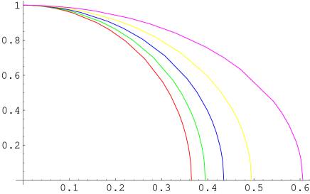
Figure 9: Sketch of the $(Q_{p-2}/M,Q_{p}/M)$ boundary of stability for $p=0$ (red), $p=1$ (green), $p=2$ (blue), $p=3$ (yellow), $p=4$ (pink). The bound state is unstable in the region below the boundary of stability.

6.2.4 The D$(p-4)$-D$p$ system

Similar statements apply to the D$p$-D$(p-4)$ bound states, which are quarter BPS in the extremal case. The supergravity solution for these states appears already in Section 5.3. Again, one can apply the CSC to find the stability pattern for these states with a simple calculation in thermodynamics. As above, we are instructed to work in a mixed canonical/grand canonical ensemble, where we allow $Q_{p-4}$ to vary holding $Q_{p}$ fixed.

In a suitable parametrization (see [61]) the thermodynamic variables of the D$(p-4)$-D$p$ system take the form

$$\begin{array}[]{c}M=\frac{V_{p}\Omega_{8-p}}{16\pi G}\frac{r_{0}^{7-p}}{2}(2+(7-p)(\cosh 2\alpha_{p}+\cosh 2\alpha_{p-4}))~{},~{}~{}T=\frac{7-p}{4\pi r_{0}\cosh\alpha_{p}\cosh\alpha_{p-4}}~{},\\[11.38109pt] S=\frac{V_{p}\Omega_{8-p}}{4G}r_{0}^{8-p}\cosh\alpha_{p}\cosh\alpha_{p-4}~{},~{}~{}\nu_{p}=\tanh\alpha_{p}~{},~{}~{}\nu_{p-4}=\tanh\alpha_{p-4}~{},{}{}\\[11.38109pt] Q_{p}=\frac{(7-p)V_{p}\Omega_{8-p}}{32\pi G}r_{0}^{7-p}\sinh 2\alpha_{p}~{},~{}~{}Q_{p-4}=\frac{(7-p)V_{p}\Omega_{8-p}}{32\pi G}r_{0}^{7-p}\sinh 2\alpha_{p-4}~{}.\end{array}$$ (6.25)

Consequently, the determinant of the Hessian matrix becomes

$$\det H_{M}=\frac{{\partial}(T,\nu_{p-4})}{{\partial}(S,Q_{p-4})}=$$ (6.26)

$$=-\frac{8G^{2}}{V_{p}^{2}\Omega^{2}_{8-p}}\frac{r_{0}^{2(p-8)}{\rm sech}^{2}\alpha_{p}{\rm sech}^{4}\alpha_{p-4}}{\cosh 2\alpha_{p-4}(7-p+2\cosh 2\alpha_{p})+(7-p)\cosh 2\alpha_{p}}(7-p-(5-p)\cosh 2\alpha_{p})~{}.$$

In this expression all the factors have a positive definite sign except for the last.

There are three values of interest for $p$. $p=4$ represents the D0-D4 bound state, for which we find an instability when

$$\cosh 2\alpha_{4}<3~{}.$$ (6.27)

The existence of a corresponding threshold unstable mode in the classical stability analysis of this bound state was argued in [60]. For $p=5$ and $p=6$ there is no stability boundary and the bound state is unstable all the way up to extremality.

6.2.5 Other examples

Other examples of bound states can be obtained from the above in the following manner. For instance, by S-dualizing the D1-D3 bound state we can obtain the F1-D3 bound state. This state exhibits the same thermodynamics as the D1-D3 system and therefore also the same stability pattern. We can also lift the D2-D4 bound state to the M2-M5 system. By further reducing the latter on a different circle we obtain the F1-D4 bound state. All three of these bound states have the same thermodynamics and the same stability pattern. Unfortunately, we cannot use T-duality to extend this list even further. As already pointed out, T-duality acts non-trivially on the CSC. On the level of the classical stability analysis the translation invariance is broken explicitly by the threshold unstable mode along the direction of the Gregory-Laflamme instability thus making it impossible to perform a T-duality transformation along these directions. On the level of thermodynamics, the same effect reappears in some cases as a change of the ensemble.

One can also consider independently the general F1-D$p$ bound state or three-charge bound states like the D0-D4-F1 system. The former was considered in [61] and the latter in [60].

Beyond these cases it would be interesting to consider the CSC in a wider class of examples, for instance in cases that exhibit rotation, such as spinning bound states.

6.3 Towards a proof of the conjecture and known counterexamples

The correlated stability conjecture has proven to be a rather robust statement whose validity has been verified in a large class of examples. A semi-classical proof of the conjecture for magnetically charged black brane solutions was given in [64] by Reall (see also [65]). Elements of this proof for more complicated systems, like that of electrically charged smeared black branes, were discussed in [61] and [66] (see also [149] for another approach to a proof based on holography). Recently [67] presented a set of counterexamples in solutions with scalar hair, which suggest that the conjecture cannot survive in its current form as a statement that applies to the most general case. To see what may go wrong, it is instructive to review the key elements of the existing arguments in favor of the CSC, the weak points of these arguments and the known counterexamples.

To expedite the discussion let us denote again by $\{z^{i}\}$ the infinite extent directions along which a Gregory-Laflamme instability can occur and by $x^{\mu}$ all the other space-time directions. For compactness, it is also convenient to denote the field content of the theory collectively by the fields $\Psi^{I}$. $I$ is a multi-index label that summarizes all the metric components and any other fields including scalar fields ($e.g.$ the dilaton) and gauge fields. The central object in the semi-classical argument of Reall [64] is the Euclidean path integral dimensionally reduced along $z^{i}$. The Euclidean path integral can be written compactly as

$$Z=\int d[\Psi^{J}]e^{-I[\Psi^{J}]}~{},$$ (6.28)

where $I[\Psi^{J}]$ is the Euclidean action and the path integral is taken over the fields $\Psi^{I}$ in the appropriate thermodynamic ensemble specified (for a class of examples) in Section 6.1. For gravity this is always the canonical ensemble and the path integral is taken over all the smooth Riemannian geometries that are asymptotically $S^{1}\times{\cal M}$. $S^{1}$ is the Euclidean time circle with circumference $\beta=\frac{1}{T}$ and ${\cal M}$ the asymptotic spatial manifold.

The Euclidean path integral is well-defined in the semi-classical approximation, where one looks for saddle points of the Euclidean action. We can expand the fields $\Psi^{I}$ around the saddle points

$$\Psi^{I}=\Psi^{I}_{0}+\delta\Psi^{I}$$ (6.29)

and write the perturbed action as

$$I[\Psi^{I}]=I_{0}[\Psi^{I}]+\delta_{2}I[\Psi^{I}]~{}.$$ (6.30)

The first order perturbation vanishes by the equations of motion and the second order perturbation can be written in terms of the Euclidean Lichnerowicz operator $\Delta_{L}$ as

$$\begin{array}[]{c}\delta_{2}I[\Psi^{I}]=\frac{1}{2}\int d^{d}xd^{d}x^{\prime}\sqrt{g_{0}}\delta\Psi^{I}(x)\frac{\delta^{2}I}{\delta\Psi^{I}(x)\delta\Psi^{J}(x^{\prime})}\delta\Psi^{J}(x^{\prime})=\\[11.38109pt] =\int d^{d}x\sqrt{g_{0}}\delta\Psi^{I}(x)(\Delta_{L})_{IJ}\delta\Psi^{J}(x^{\prime})~{}.\end{array}$$ (6.31)

The Euclidean path integral $Z$ receives two contributions: one from the saddle point configuration and another from the determinant of the Lichnerowicz operator, so

$$Z\propto(\det\Delta_{L})^{-1/2}e^{-I_{0}[\Psi^{I}_{0}]}~{}.$$ (6.32)

When the Lichnerowicz operator has a negative eigenvalue, in other words when the system of differential equations

$$(\Delta_{L})_{IJ}\delta\Psi^{J}=\lambda{\cal G}_{IJ}\delta\Psi^{J}$$ (6.33)

has a solution with $\lambda<0$, the Euclidean path integral $Z$ receives an imaginary contribution, which can be seen as a signal of thermodynamic instability. ${\cal G}_{IJ}$ is a natural metric on the space of perturbations defined implicitly by (6.33).

The existence of a negative eigenvalue for the dimensionally reduced Euclidean Lichnerowicz operator provides a natural bridge between classical and local thermodynamic instability. The connection to a classical instability of the Lorentzian theory arises in the following way. As we found in previous sections, a clear signal of a dynamical instability is the existence of a threshold unstable mode. Let us denote this threshold mode as $\delta\psi^{I}$. We can separate the $z^{i}$ dependence of this mode by setting

$$\delta\psi^{I}={\rm Re}\left(e^{ik_{j}z^{j}}\delta\Psi^{I}\right)~{}.$$ (6.34)

Plugging this ansatz into the second order perturbation of the equations of motion of the theory leads to a system of differential equations of the form

$$(\hat{\Delta}_{L})_{IJ}\delta\Psi^{J}=-k^{2}{\cal G}_{IJ}\delta\Psi^{J}~{},$$ (6.35)

where $(\hat{\Delta}_{L})_{IJ}$ is the dimensionally reduced Lorentzian Lichnerowicz operator (see (2.21)). After a trivial Wick rotation equation (6.35) becomes (6.33) with $\lambda=-k^{2}$. Hence, we see that there is a close relation between the negative modes appearing in the dimensionally reduced Euclidean path integral and the momentum of the threshold unstable modes of the classical stability analysis.

On the other hand, one can argue for a natural relation between the semi-classical path integral and local thermodynamic stability. To make this relation more precise Reall suggested an argument, based on an earlier construction given in [150, 151]. The goal of the argument is to relate the Hessian $\frac{\delta^{2}I}{\delta\Psi^{I}\delta\Psi^{J}}$ of the action $I$ with the Hessian $H_{M}$ of the local thermodynamic stability analysis. For that purpose, consider a system with temperature $T$, entropy $S$ and $n$ additional charges $Q_{i}$. The $n$ corresponding chemical potentials will be denoted as $\nu_{i}$. In terms of these variables the first law of thermodynamics takes the form

$$dM=TdS+\sum_{i}\nu_{i}dQ_{i}~{}.$$ (6.36)

In the grand canonical ensemble, the idea is to construct an $n+1$-parameter family of configurations with Euclidean action

$$I(x_{0},...,x_{n};\beta,\nu_{1},....,\nu_{n})=\beta M(x_{0},...,x_{n})-S(x_{0},...,x_{n})-\beta\sum_{j=1}^{n}\nu_{j}Q_{j}(x_{0},...,x_{n})~{}.$$ (6.37)

The generic point in this family is an off-shell background, which does not satisfy the Einstein equations of motion, but satisfies the appropriate Hamiltonian constraints. For a particular value of the $n+1$ parameters $(x_{0},....,x_{n})=(x_{0}(\beta,\nu_{1},...,\nu_{n}),...,x_{n}(\beta,\nu_{1},....,\nu_{n}))$ the background becomes an exact solution of the equations of motion. At this point the functions $M,S$ and $Q_{i}$ are precisely the energy, entropy and charges of the corresponding gravitational system. For other values of the parameters $(x_{0},...,x_{n})$ the interpretation of the functions $M,S$ and $Q_{i}$ is not important.

Given the existence of such a family of configurations, we can immediately draw a number of interesting conclusions. First of all, since the configurations become an exact solution of the equations of motion at the special point

$$P=(x_{0},....,x_{n})=(x_{0}(\beta,\nu_{1},...,\nu_{n}),...,x_{n}(\beta,\nu_{1},....,\nu_{n}))$$

the action $I$ is extremized there yielding

$$\left(\frac{{\partial}I}{{\partial}x_{j}}\right)_{\beta,\nu_{1},...,\nu_{n}}=0~{},~{}~{}j=0,...,n~{}$$ (6.38)

or equivalently the standard thermodynamic relations

$$\frac{1}{\beta}=\left(\frac{{\partial}M}{{\partial}S}\right)\bigg{|}_{(x_{0},...,x_{n})=P}~{},~{}~{}\nu_{i}=\left(\frac{{\partial}M}{{\partial}Q_{i}}\right)\bigg{|}_{(x_{0},...,x_{n})=P}~{},~{}~{}i=1,...,n~{}.$$ (6.39)

The quadratic perturbation of the action $I$ around the special point $P$ involves the Hessian matrix $I_{(2)}=\frac{{\partial}^{2}I}{{\partial}x_{j}{\partial}x_{k}}$, which can be recast in terms of the Hessian matrix $H_{M}$ as

$$\left(I_{(2)}\right)_{ab}=M_{a}^{~{}\alpha}\left(H_{M}^{-1}\right)_{\alpha\beta}M^{\beta}_{~{}b}~{}.$$ (6.40)

In this relation, which can be deduced easily with the use of the first order equations (6.38), $M_{a}^{~{}\alpha}$ is the Jacobian matrix of the transformation from the variables $(x_{0},...,x_{n})$ to the thermodynamic variables $(\beta,\nu_{1},...,\nu_{n})$. Therefore, assuming $M$ to be an invertible matrix, we can use equation (6.40) to achieve the desired relation between the Hessian matrix $I_{(2)}$ of classical stability and the Hessian matrix $H_{M}$ of local thermodynamic stability.

The construction of the $n+1$ parameter family of configurations is a non-trivial exercise that has not been performed for the most general system. So far the construction has been performed explicitly for magnetically charged black brane solutions in [64] and for electrically charged smeared black branes in [66].

To complete the proof one has to verify an additional set of properties. For instance, one should verify that the norm of the on-shell perturbations on the space of theories is positive definite. This ensures that the analysis is restricted to normalizable on-shell perturbations excluding for example any non-physical negative-norm conformal perturbations. The positivity of the norm

$$||\delta\Psi||^{2}=\int d^{d}x~{}\delta\Psi^{I}{\cal G}_{IJ}\delta\Psi^{J}$$

also ensures that the action $I$ decreases, and therefore an instability exists, precisely when the Hessian $\frac{\delta^{2}I}{\delta\Psi^{I}\delta\Psi^{J}}$ fails to be positive definite (see equations (6.31), (6.33)).

Finally, one should demonstrate that there is sufficient overlap between the off-shell deformations $(x_{0},...,x_{n})$ with the actual on-shell perturbations $\delta\psi^{I}$. In [64] it was pointed out that a path in the family of off-shell configurations is not related directly to an eigenfunction of the Lichnerowicz operator, but rather some linear combination of eigenfunctions. This suggests that when the action decreases along this path, at least one of the eigenvalues of the Lichnerowicz operator must be negative and therefore an actual on-shell instability should exist. It is not immediately obvious, however, that the converse is also true. To complete the proof one should demonstrate that the off-shell deformations and the actual on-shell perturbations cover the same linear space. This is a rather subtle point that has not been demonstrated fully in any known example. It is natural to expect in general that there will be sufficient overlap between the eigenfunctions of the Lichnerowicz operator and the family of off-shell deformations for systems that are specified uniquely by a complete set of conserved charges. Systems with hair do not fall into this category and are therefore the prime candidates as systems that violate the CSC in its current formulation. In such situations the full set of conserved charges is not enough to determine uniquely the classical solution. As we saw the conserved quantities are the only input of the local thermodynamic stability; a dynamical instability, however, is a property of the entire solution.

This crucial point was put forward in [67], which presented a set of theories where the exact black brane solutions are specified by a set of conserved charges and the asymptotic values of a set of scalar fields. It was found that these systems can develop a classical instability associated with the dynamics of the scalar fields despite the presence of local thermodynamic stability.

The violation of the CSC observed in [67] is reminiscent of an earlier counterexample proposal in [152]. The central objects in that paper are three-charge D1-D5-P spinning black brane solutions in type IIB supergravity compactified on $T^{4}$. This class of solutions contains gyrating black strings [153] carrying the same charges as ordinary spinning black strings, but a different value of an extra parameter, which measures the angular momentum carried by gyrations of the string (as opposed to spin). [152] argued that a small perturbation of a non-gyrating black string could grow to become large for sufficiently large angular momentum. This new instability was proposed as a possible counterexample to the CSC.

Given the explicit violation of the CSC in the above examples, is it still possible to find a suitable refinement or restriction of the conjecture that can survive as a correct statement? The above counterexamples suggest two natural possibilities. If we choose to leave the definition of local thermodynamic stability unchanged in the formulation of the conjecture, then it is natural to add a further assumption and conjecture that the CSC works provided that there is a unique solution with a spatially uniform horizon and specified conserved charges [67]. No counterexamples of this restricted version of the CSC are known. An alternative, more ambitious, refinement of the conjecture has been suggested by B. Kol (see [67]). We can redefine the meaning of local thermodynamic stability by enlarging the Hessian matrix to include derivatives with respect to those quantities that characterize the asymptotics of the scalar fields or any other quantity that determines uniquely a solution. In that case, local thermodynamic stability translates into a positivity criterion for the new enlarged Hessian matrix. It seems quite likely that with this refinement the CSC survives all tests known up to date.

7 Holographic implications

Holography provides a non-trivial relation between a gravitational theory in the bulk and a non-gravitational theory ($e.g.$ a Yang-Mills theory) on the boundary. A well-known example of this relation is the AdS/CFT correspondence between the $\mathcal{N}=4$ Super-Yang-Mills theory and type IIB string theory on $AdS_{5}\times S^{5}$ [19, 20, 21, 80]. In general, holography relates gravity in the near-horizon background of a brane configuration in string/M-theory and the non-gravitational world-volume theory living on the branes in a low-energy decoupling limit [22].

In this section we discuss gauge/gravity duals in which the gravity side exhibits a Gregory-Laflamme instability. The presence of this classical gravitational instability in the bulk has important consequences for the gauge theory on the boundary, which we review following [56, 57, 155, 66, 58]. Focusing on a set of examples that are closely connected to the material of this review we will consider first D-branes on a circle, where the relevant gauge theory is super-Yang-Mills theory on a circle. This example can be generalized with D-branes on higher-dimensional torii, which we discuss briefly at the end of the first subsection. Other interesting examples include the M2- and M5-brane on a circle, where the relevant non-gravitional theory is (2+1)-dimensional super-Yang-Mills and Little String theory. We review the basic features of both cases giving more emphasis to the second example, which exhibits new properties not present in the other cases. We conclude with a brief discussion of the implications of Gregory-Laflamme instabilities for non-commutative Yang-Mills and non-commutative open string theories, which arise as part of the worldvolume dynamics of D-brane bound states.

7.1 D-branes on a circle

Consider the supergravity solution of a large number of coincident D$(p-1)$-branes on a transverse circle. In Section 5.1 we found that there is a map between the phases of neutral Kaluza-Klein black holes (see Section 3) and the phases of non- and near-extremal D-branes on a transverse circle. Furthermore, we saw in Section 5.2 that we can map the Gregory-Laflamme mode of the neutral black string to a Gregory-Laflamme mode of non- and near-extremal D-branes smeared on a transverse circle. In this section we will discuss the consequences of this unstable mode for the holographically dual theories living on the D-branes.

The low-energy theory on $N$ coincident D$p$-branes in type II string theory in flat space is given by the $(p+1)$-dimensional $U(N)$ super-Yang-Mills theory with sixteen supercharges (on $\mathbb{R}^{p,1}$). According to holography [19, 22], the large $N$, finite temperature, $SU(N)$ version of this theory is equivalent to the near-extremal limit of the supergravity solution of $N$ coincident D$p$-branes. The perturbative Yang-Mills description is valid at small ’t Hooft coupling and the supergravity description at large ’t Hooft coupling.

Similarly, since a near-extremal D$(p-1)$-brane on a transverse circle is T-dual to a D$p$-brane wrapped on a circle we conclude that the gauge theory dual of $N$ coincident near-extremal D$(p-1)$-branes on a transverse circle is $(p+1)$-dimensional SYM on $\mathbb{R}^{p-1,1}\times S^{1}$ with gauge group $SU(N)$ and sixteen supercharges [156, 157, 158, 159, 160, 161].

For example, this implies a correspondence between the phases of near-extremal D2-branes on a transverse circle and the phases of ${\cal{N}}=4$ SYM theory on $\mathbb{R}^{2,1}\times S^{1}$ . By Wick rotating to Euclidean space, where the non-zero temperature translates to a compact direction, we get ${\cal N}=4$ SYM on $\mathbb{R}^{2}\times\mathbb{T}^{2}$, the two-torus being $\mathbb{T}^{2}\equiv S_{\beta}^{1}\times S^{1}$. Two other interesting examples are near-extremal D0- and D1-branes on a transverse circle. These are respectively dual to $(1+1)$-dimensional SYM theory on $\mathbb{T}^{2}=S_{\beta}^{1}\times S^{1}$ and to $(2+1)$-dimensional SYM on $\mathbb{R}\times\mathbb{T}^{2}$ (in Euclidean space). In what follows we will restrict the discussion to the cases of D0-, D1-, D2- and D3-branes on a circle, but one should keep in mind that the results of this section can be easily extended to include the F-strings and the remaining D-branes.

The main point of the discussion here is that we can use the gravity results of Sections 5.1 and 5.2 to obtain predictions for the thermodynamics of the dual strongly coupled gauge theories described in the previous paragraphs [56, 57, 66, 58]. We will see, for example, that the localized phase of the supergravity phase diagram corresponds to the low temperature/low energy regime of gauge theory, while the non-uniform phase corresponds to a new phase that emerges from the uniform phase. The latter describes the high temperature/high energy regime of gauge theory. The Gregory-Laflamme instability in supergravity has a natural counterpart in gauge theory as an instability of the high energy/temperature phase when the energy/temperature becomes sufficiently low.

The dictionary between the supergravity parameters of the near-extremal D$p$-branes on a (transverse) circle and the parameters of SYM theory has been established in Section 5. We summarize it here for the convenience of the reader. On the gravity side, $L$ and $\hat{L}$ denote respectively the circumference of the transverse circle and its T-dual. $g_{s}$ and $\hat{g}_{s}$ denote the string coupling in the theory before and after T-duality. These quantities are related to each other via the relations (5.47). On the gauge theory side, $N$ is the rank of the $SU(N)$ gauge group and $\lambda=g_{\rm YM}^{2}N=(2\pi)^{p-2}\hat{g}_{s}l_{s}^{p-3}$ the ’t Hooft coupling. The energy and temperature of the field theory will be denoted by $E$ and $\hat{T}$ respectively. The definition of the near-extremal limit (5.19) on the gravity side involves two parameters $g$ and $l$, which are kept fixed. These parameters can be re-expressed in terms of the SYM variables in the following way

$$g=\frac{1}{(2\pi)^{3}N^{2}}\frac{\hat{L}^{p}}{V_{p-1}}\left(\lambda\hat{L}^{3-p}\right)^{2}\ ,\ \ l=\frac{\hat{L}}{\sqrt{2\pi}}\sqrt{\lambda\hat{L}^{3-p}}\ .$$ (7.1)

From $g$, $l$ and $\hat{T}$ we can form two independent dimensionless parameters, $l/g$ and $l\hat{T}$, which will play an important role below. These parameters are functions of the dimensionless temperature and coupling $t^{\prime}=\hat{L}\hat{T}$, $\lambda^{\prime}=\lambda\hat{L}^{3-p}$.

It should be noted that stringy corrections to the supergravity description of coincident D$p$-branes wrapping a circle

$$l_{s}^{-2}ds^{2}=\frac{R^{\frac{7-p}{2}}}{\sqrt{\hat{h}_{d}}}\left[-\left(1-\frac{R_{0}^{7-p}}{R^{7-p}}\right)dt^{2}+\frac{d\hat{z}^{2}}{(2\pi)^{2}}\right]+\frac{\sqrt{\hat{h}_{d}}}{R^{\frac{7-p}{2}}\left(1-\frac{R_{0}^{7-p}}{R^{7-p}}\right)}dR^{2}+\sqrt{\hat{h}_{d}}R^{\frac{p-3}{2}}d\Omega^{2}_{8-p}$$

are negligible when the string scale is small compared to the length scale generated at the horizon $\ell_{H}\sim\sqrt{\alpha^{\prime}}\hat{h}^{1/4}R_{0}^{\frac{p-3}{4}}L^{-\frac{1}{2}}$, $i.e.$ when $\ell_{H}\gg\sqrt{\alpha^{\prime}}$. This is equivalent (up to a constant factor with powers of $\pi$ that we drop) to the condition $\hat{L}\hat{T}\ll(\lambda\hat{L}^{3-p})^{\frac{1}{3-p}}$. On the other hand, the typical mass of the winding modes is $M_{w}\sim\frac{R_{0}^{(7-p)/2}L^{1/2}}{\sqrt{\alpha^{\prime}}\hat{h}^{1/4}}$, so the effects of the winding modes can be neglected when $\ell_{H}M_{w}\gg 1$, $i.e$ when $R_{0}\gg 1$. This is equivalent to $\hat{L}\hat{T}\gg(\lambda\hat{L}^{3-p})^{-\frac{1}{2}}$. Hence, when $p=1,2$ and $\lambda^{\prime}=\lambda\hat{L}^{3-p}\gg 1$ the supergravity solution 7.1 is valid for a large range of temperatures $t^{\prime}$. For $p=3$ the supergravity solution is valid when ${\lambda^{\prime}}^{-\frac{1}{2}}\ll t^{\prime}\ll 1$ and for $p=4$ when ${\lambda^{\prime}}^{-\frac{1}{2}}\ll t^{\prime}\ll{\lambda^{\prime}}^{-1}$. The latter condition implies $\lambda^{\prime}\ll 1$.

In a similar fashion, the T-dual background of smeared D$(p-1)$ branes (see Eqs. (5.26)-(5.28)) is valid ($i.e.$ stringy and winding mode corrections can be ignored) when $t^{\prime}\ll{\lambda^{\prime}}^{\frac{1}{3-p}}$, $t^{\prime}\ll 1$.

Having said this, we are now ready to use the supergravity results of Section 5 to make definite predictions for the phase diagram of the dual gauge theory at strong coupling. For that purpose we recast the thermodynamics of Section 5 in terms of gauge theory variables. In (5.24) we defined and computed the rescaled energy, temperature, entropy and free energy quantities $\epsilon$, $\hat{\mathfrak{t}}$, $\hat{\mathfrak{s}}$ and $\hat{\mathfrak{f}}\equiv\epsilon-\hat{\mathfrak{t}}\hat{\mathfrak{s}}$. In terms of these variables we obtain the dual gauge theory entropy and free energy $\hat{S}$ and $\hat{F}$ by reinstating the dimensions

$$\hat{S}(E)=\frac{l}{g}\hat{\mathfrak{s}}(gE)\ ,\ \ \hat{F}(\hat{T})=\frac{1}{g}\hat{\mathfrak{f}}(l\hat{T})~{}.$$ (7.3)

In the ensuing we concentrate mostly on the canonical ensemble and summarize the phases of ($p+1$)-dimensional SYM theory on $\mathbb{R}^{p-1,1}\times S^{1}$ that follow from the uniform, localized and non-uniform phases of near-extremal D$(p-1)$-branes in supergravity.

7.1.1 Uniform phase: High temperature phase of SYM on a circle

The uniform phase of near-extremal D$(p-1)$-branes on a circle corresponds to the high temperature phase of ($p+1$)-dimensional SYM theory on $\mathbb{R}^{p-1,1}\times S^{1}$. This is physically sensible because high temperatures correspond to short distances. In this regime the details of the compact direction in $\mathbb{R}^{p-1,1}\times S^{1}$ are invisible and the circumference $\hat{L}$ appears only as a trivial proportionality factor in the free energy. This is precisely what we find in the uniform phase that corresponds to a uniformly smeared near-extremal D$(p-1)$-brane (recall that this solution has the same thermodynamics as a near-extremal D$p$-brane wrapping the T-dual circle). We can check this statement explicitly using the thermodynamics (5.30) and the dictionary (7.3). The resulting free energy is

$$\hat{F}^{\rm u}_{{\rm SYM}(p+1)}(\hat{T})=\hat{F}^{\rm u}_{{\rm D}(p-1)}(\hat{T})=-k_{p}V_{p-1}\hat{L}N^{2}\lambda^{-\frac{3-p}{5-p}}\hat{T}^{2\frac{7-p}{5-p}}\ ,$$ (7.4)

where the coefficients $k_{p}$ are given in Table 5. The expression (7.4) is indeed the familiar result for the free energy of the D$p$-brane theory, with $V_{p}=V_{p-1}\hat{L}$.

7.1.2 Localized phase: Low temperature phase of SYM on a circle

The localized phase corresponds to the low temperature phase of ($p+1$)-dimensional SYM theory on $\mathbb{R}^{p-1,1}\times S^{1}$. Low temperatures correspond to large distances in the SYM theory, so in this regime the presence of the circle enters in a non-trivial manner and the whole tower of Kaluza-Klein states can contribute. We will see that as we send the temperature to zero, the leading order thermodynamics is captured by the thermodynamics of the near-extremal D$(p-1)$-brane, which is dual to the strongly coupled $p$-dimensional SYM theory on $\mathbb{R}^{p-1,1}$. The next-to-leading order corrections to the thermodynamics of the localized phase (see Section 5.1) will lead to gauge theory corrections that capture the contribution of the Kaluza-Klein modes on the circle.

Using the expressions for the corrected free energy in (5.37) together with the dictionary (7.1), (7.3) we deduce that the free energy of the localized phase of thermal ($p+1$)-dimensional SYM theory on $\mathbb{R}^{p-1,1}\times S^{1}$ is

$$\hat{F}^{\rm loc}_{{\rm SYM}(p+1)}(\hat{T})=\hat{F}^{\rm loc}_{{\rm D}(p-1)}(\hat{T})$$ (7.5)

$$\simeq-k_{p-1}V_{p-1}N^{2}\left(\frac{\lambda}{\hat{L}}\right)^{-\frac{4-p}{6-p}}\hat{T}^{2\frac{8-p}{6-p}}\left\{1+\frac{2(9-p)\zeta(8-p)k_{p-1}}{(6-p)^{2}(2\pi)^{3}\Omega_{9-p}}\left[\hat{L}\hat{T}\sqrt{\lambda\hat{L}^{3-p}}\right]^{2\frac{8-p}{6-p}}\right\}\ .$$

The coefficients $k_{p}$ are the same as above and are listed in Table 5.

$p$	0	1	2	3	4
$k_{p}$	$(2^{21}3^{2}5^{7}7^{-19}\pi^{14})^{1/5}$	$2^{4}3^{-4}\pi^{5/2}$	$(2^{13}3^{5}5^{-13}\pi^{8})^{1/3}$	$2^{-3}\pi^{2}$	$2^{5}3^{-7}\pi^{2}$

Table 5: Coefficients for the free energy of D$p$-branes.

Notice that the leading term in (7.5) is in perfect agreement with the expected result for the strong coupling limit of the $p$-dimensional SYM theory. In particular, the ’t Hooft coupling appears through the combination $\lambda/\hat{L}$, which is precisely what we expect to find by compactifying the $(p+1)$-dimensional theory with ’t Hooft coupling $\lambda$. The second term in (7.5) gives a quantitative prediction for the first correction in terms of the dimensionless parameter

$$\delta=\hat{L}\hat{T}\sqrt{\lambda\hat{L}^{3-p}}\ .$$ (7.6)

The next corrections will be of order $(\delta^{2\frac{8-p}{6-p}})^{2}$. It would be very interesting to reproduce these corrections from the field theory side. We refer the reader to [57] for the explicit expressions of (7.5) in the cases $p=1,2,3$ and 4.

Similar results in the microcanonical ensemble can be easily obtained using the corrected entropy (5.35) of the localized near-extremal branes and (7.1), (7.3).

7.1.3 Non-uniform phase: New phase in SYM on a circle

The non-uniform phase of near-extremal $D(p-1)$-branes on a circle (see Section 5.1) predicts the existence of a new phase of ($p+1$)-dimensional SYM theory on $\mathbb{R}^{p-1,1}\times S^{1}$ at intermediate temperatures. With the use of (5.33) and the dictionary (7.1), (7.3) we can also deduce the first correction to the thermodynamics around the point where the non-uniform phase connects to the uniform phase. One finds the free energy

$$F^{\rm nu}_{{\rm SYM}(p+1)}(\hat{T})=F^{\rm nu}_{{\rm D}(p-1)}(\hat{T})$$ (7.7)

$$\simeq-(2\pi)^{3}V_{p-1}N^{2}\lambda\hat{L}^{3-2p}\left[\frac{5-p}{9-p}\epsilon_{c}+\hat{\mathfrak{t}}_{c}\hat{\mathfrak{s}}_{c}\left(\frac{\hat{T}}{\hat{T}_{c}}-1\right)+\frac{\hat{\mathfrak{t}}_{c}c}{2}\left(\frac{\hat{T}}{\hat{T}_{c}}-1\right)^{2}\right]\ .$$

The critical temperature in this expression is given by

$$\hat{T}_{c}=\frac{\hat{\mathfrak{t}}_{c}}{\hat{L}}\sqrt{\frac{2\pi}{\lambda\hat{L}^{3-p}}}\ .$$ (7.8)

and the values for $\hat{\mathfrak{t}}_{c}$, $\epsilon_{c}$, $\hat{\mathfrak{s}}_{c}$ and $c$ can be read off from Table 4 by using $d=10-p$. Notice that the first term in the expression (7.7) corresponds to $\hat{F}^{\rm u}_{{\rm SYM}(p+1)}(\hat{T}_{c})$, $i.e.$ the free energy (7.4) of the uniform phase evaluated at the critical temperature. The second term is $-\hat{S}^{\rm u}_{{\rm SYM}(p+1)}(\hat{T}_{c})(\hat{T}-\hat{T}_{c})$ and therefore involves the entropy of the uniform phase evaluated at the critical temperature. The third term contains the departure of the free energy from the uniform phase into the non-uniform phase. It would be very interesting to understand the results (7.5) and (7.7) for thermal $(p+1)$-dimensional SYM theory on $\mathbb{R}\times\mathbb{R}^{p-1}\times S^{1}$ from the gauge theory side.

Again, similar results for the non-uniform phase in the microcanonical ensemble can be obtained using the corrected entropy (5.32) of the localized near-extremal branes and (7.3), (7.1).

Finally, since both the localized and non-uniform phase of near-extremal branes have copies, we also have copies of the thermal $(p+1)$-dimensional SYM phases obtained above. See Ref. [57] for further details.

7.1.4 The expected T(E) diagram for D-branes on a circle

As we discussed above, the thermodynamics of near-extremal D$p$-branes on a transverse circle, is related to the thermodynamics of phases of Kaluza-Klein black holes in $10-p$ dimensions. In particular, for the cases of interest in this section, namely D0, D1, D2 and D3-branes, we need the phases of Kaluza-Klein black holes in 10, 9, 8 and 7 dimensions. However, at present we do not have complete analytical or numerical data (see, however [33]) for the localized and non-uniform phases in those dimensions. For this reason, our results so far ($c.f.$ the free energies (7.5) and (7.7) for the localized and non-uniform phase respectively) have been leading order results around some specific point in the phase diagram. For the localized phase this point is the origin (large radius limit) and for the non-uniform phase it is the GL point. For the uniform phase we have of course the exact result (7.4).

Nevertheless, based on the expectation that the $(\mu,n)$ phase diagram for neutral Kaluza-Klein black holes in those dimensions has a similar form as those in 5 and 6 dimensions (see Fig. 3) we can use the map (5.23) to make some general observations [58]. For example, the map implies that the $(E,r)$ phase diagram for the near-extremal D$p$-branes has the same qualitative form as that in Fig. 3. From this we get a prediction for the qualitative form of the $T(E)$ diagram, because given the curves in the $(E,r)$ phase diagram the entire thermodynamics is determined.

For instance, consider the case of $N$ near-extremal D2-branes on a transverse circle, which is dual to finite temperature ${\cal N}=4$ supersymmetric $SU(N)$ Yang-Mills on $\mathbb{R}^{2}\times\mathbb{T}^{2}$. A similar qualitative picture is expected also for the other D$p$-brane cases. In the uniform phase, which consists of near-extremal D2-branes uniformly smeared on a transverse circle, the relation between temperature and energy is

$$T(E)\propto E^{\frac{1}{4}}\ ,$$ (7.9)

We argued that the uniform phase dominates at high energies. In the localized branch which dominates at low energies we know [57] that the temperature/energy relation is

$$T(E)\propto E^{\frac{3}{10}}(1+\alpha E)\ ,\ \ E\ll 1\ ,$$ (7.10)

with $\alpha<0$ a known constant. Finally, there is a non-uniform phase which emanates from the uniform phase at the critical energy $E_{\rm c}=0.71\cdot(2\pi)^{3}V_{2}N^{2}/(\lambda\hat{L}^{3})$. At the critical point, the ratio of the specific heat of the non-uniform phase to the specific heat of the uniform phase is [57]

$$\frac{c_{\rm nu}}{c_{\rm u}}=\frac{1}{1+\frac{6}{7}\hat{\gamma}\epsilon_{c}}=0.41\ .$$ (7.11)

The ratio is less than one, a feature that holds for any of the D$p$-brane cases mentioned above.

The salient features of the emerging picture in the $T(E)$ diagram are the following

• Both the uniform and localized phases begin at the origin (with infinite slope) and at very low energies the uniform phase has higher temperature than the localized phase (at a given energy). As the energy is increased the localized phase is expected to cross the uniform phase at relatively low energies below the critical energy where the non-uniform phase emerges.

• The slope in the $T(E)$ diagram is the inverse of the specific heat. Therefore we deduce from (7.11) that the slope of the non-uniform phase at the critical point $(E,T)=(E_{\rm c},T_{\rm c})$ is larger than that of the uniform phase.

• It is natural to assume that the localized and non-uniform branches meet at a merger point in a qualitatively similar way to the one observed explicitly in the NS5-brane case in [58] (see Fig. 12).

The emerging picture is summarized in Fig. 10.

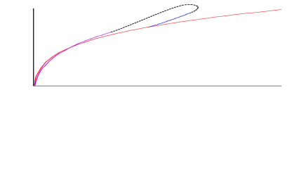
Figure 10: The qualitative picture of energy versus temperature for the phases of near-extremal D$p$-branes on a transverse circle. One can see the uniform (red), non-uniform (blue) and localized (magenta) phases. The dashed curve connects the localized and non-uniform phase.

We notice that as we increase the energy above extremality in the localized phase we first reach a point where the specific heat becomes infinite. This is the point where the localized phase attains its maximal temperature. Increasing the energy further we reach a point where the specific heat vanishes. This is the point where the localized phase attains its maximal energy. Despite the presence of a maximal temperature in the localized phase, the uniform phase exists for any temperature and therefore no limiting temperature exists for the system of near-extremal branes on a circle. Hence, for sufficiently high temperatures the system will necessarily find itself in the uniform phase. At low temperatures the localized phase will be favored.

The above behavior is the same in both the canonical and microcanonical ensembles. In Section 7.2.2 we will see that the case of NS5-branes is very different in this respect. In that case the uniform phase has a constant Hagedorn temperature and there is a striking difference between the canonical and microcanonical ensembles.

7.1.5 From strong to weak gauge coupling

So far we have obtained a set of predictions for strongly coupled $(p+1)$-dimensional SYM theory on a circle by analyzing the supergravity phases of near-extremal black hole solutions on a transverse circle. It is interesting to ask what happens to all these phases in gauge theory when we continue the theory from strong to weak ’t Hooft coupling $\lambda$. If there is a line of phase transitions at strong coupling, this line is not expected to end abruptly in the $(\lambda,T)$ parameter space as we change the coupling $\lambda$. It may either go to zero or infinite temperature at a finite value of the coupling, or it may continue smoothly to weak coupling, where one can analyze it with standard perturbative methods directly in gauge theory. An example of the latter possibility is the Hawking-Page transition [79, 80] in $AdS_{5}$, which is dual to a thermal deconfinement transition in $(3+1)$-dimensional ${\cal N}=4$ SYM theory on $S^{3}$. This transition can indeed be continued to weak coupling where it can be analyzed explicitly [81, 82, 83]. A similar continuation to weak coupling also occurs for the case of interest in this section, namely the Gregory-Laflamme instability and the associated transition in the dual SYM theories on a circle. This has been shown for the $(1+1)$-dimensional maximally supersymmetric YM theory in [56]. We review the main features of this example in the ensuing.

The Euclidean $(1+1)$-dimensional $SU(N)$ SYM theory on the torus $S^{1}_{\beta}\times S^{1}$ has two non-contractible Wilson loops, the loops running around the time $\tau$ and circle $z$. The spatial Wilson loop

$${\cal P}_{z}=Pe^{i\oint dzA_{z}}$$ (7.12)

is of special interest here, because it serves as an order parameter for the weak coupling manifestation of the Gregory-Laflamme transition. Indeed, the eigenvalues of ${\cal P}_{z}$ represent the positions of T-dual D0-branes on a circle and their distribution can distinguish between the three different phases. The uniform phase corresponds to a uniform eigenvalue distribution, the non-uniform phase corresponds to a non-uniform eigenvalue distribution that breaks the translational invariance on the transverse circle and the localized phase maps to an eigenvalue distribution, which is localized on the transverse circle. [56] showed that the eigenvalue distribution of the Wilson loop ${\cal P}_{z}$ is sharply localized at small temperatures and weak coupling. As we continue the theory to higher temperatures the eigenvalues spread out and fill out the whole circle. There is a critical temperature $T_{c}\simeq 1.4/(\lambda\hat{L}^{3})$ where the theory undergoes a Gross-Witten like phase transition [124] from the localized distribution to the uniform distribution. For more details we refer the reader to the original discussion of the Refs. [56, 163].

7.1.6 Implications of the GL instability for higher tori

Above we considered the implications for Yang-Mills theory on a circle due to the Gregory-Laflamme instability of D-branes smeared on a transverse circle. Similar results can be obtained for Yang-Mills theory on a torus $\mathbb{T}^{k}$ by analyzing the Gregory-Laflamme instability of D-branes smeared on a transverse torus $\mathbb{T}^{k}$.

As a special case, consider the $\mathcal{N}=4$ SYM theory on $\mathbb{R}\times\mathbb{T}^{3}$. The holographic dual of this theory arises from D0-branes smeared on the three-torus $\mathbb{T}^{3}$. This brane configuration has Gregory-Laflamme instabilities in the periodic directions when the radii are sufficiently large. This implies an interesting phase structure which generalizes the phase structure of non-extremal D-branes on a circle presented in Section 5.1. First, for $\mathbb{T}^{3}=S^{1}\times\mathbb{T}^{2}$ we can obtain several phases for the D0-branes on $\mathbb{T}^{3}$ from the phases of D2-branes on a circle with T-duality, imposing that there is no dependence on the $\mathbb{T}^{2}$ directions. Thus, we inherit all the phases of the D2-brane on a circle. Moreover, it is conceivable that there are new localized phases, for example, phases in which the D0-brane horizon is topologically $S^{3}\times S^{5}$ corresponding to having the D0-branes localized in all three torus directions, or one could have that the D0-brane is localized in two directions giving an $S^{1}\times S^{2}\times S^{5}$ horizon. In addition, one can well imagine new non-uniform phases, for example in which the D0-branes are not localized in any of the three directions but nevertheless are non-uniform in all three directions. This would correspond to a $\mathbb{T}^{3}\times S^{5}$ topology of the horizon. Therefore, we see that the phase structure of D0-branes on $\mathbb{T}^{3}$ is even richer than that of D-branes on a circle. This is in accordance with the phase structure of neutral $p$-branes on tori as discussed in Section 4.3. In particular, via the boost/U-duality map discussed in Section 5.1 one can directly relate the phases of neutral Kaluza-Klein black holes on $\mathcal{M}^{1,6}\times\mathbb{T}^{3}$ to those of non- and near-extremal D0-branes smeared on $\mathbb{T}^{3}$. Through holography, the richness of the phase structure for D0-branes on $\mathbb{T}^{3}$ implies an equally rich phase structure for $\mathcal{N}=4$ SYM theory on $\mathbb{R}\times\mathbb{T}^{3}$. We refer to [163] for more considerations on the phase structure of gauge theories on tori.

7.2 M2- and M5-branes on a circle

In this section we consider separately the cases of near-extremal M2- and M5-branes on a transverse circle. By IIA/M S-duality, the former is dual to the near-extremal D2-brane and the latter is dual to the near-extremal NS5-brane. Hence, it is conjectured that $N\gg 1$ coincident near-extremal M2-branes on a circle are dual to (2+1)-dimensional SYM theory with sixteen supercharges and gauge group $SU(N)$ [19, 22]. Similarly, the system of $N\gg 1$ concident near-extremal M5-branes on a transverse circle is dual to the six-dimensional $(2,0)$ LST. In both cases, the transverse circle is the M-theory circle and the dual non-gravitational theory lives on the non-compact space $\mathbb{R}^{p,1}$. $p=2$ for the case of the M2-brane and $p=5$ for the case of the M5-brane.

7.2.1 $(2+1)$-dimensional SYM theory

In this case we place $N$ near-extremal M2-branes transverse to the M-theory circle, which we take to have circumference $L=2\pi g_{s}l_{s}$. Using the quantization condition that comes from the M2-branes together with (5.19) and (5.22) we find that we can recast the supergravity parameters $g$, $l$ as

$$g=\frac{(2\pi)^{2}}{V_{2}}\frac{N^{3}}{\lambda^{3}}\ ,\ \ l=2\pi\frac{N^{3/2}}{\lambda}\ ,$$ (7.13)

where $\lambda={g_{\rm YM}}^{2}N=g_{s}l_{s}^{-1}N$. As in the cases of the previous subsection, these relations provide a dictionary between the supergravity results of the near-extremal M2-branes on a circle and the dual $(2+1)$-dimensional SYM theory. Since there are many similarities between this case and the case of D$p$-branes on a transverse circle of the previous subsection, we will provide here only a brief summary of the main results and refer the reader to [57] for a more detailed discussion. Qualitatively similar results can be obtained in both the microcanonical and canonical ensembles.

The uniform phase of near-extremal M2-branes on a circle corresponds to the high temperature/high energy phase of thermal $(2+1)$-dimensional SYM. The localized phase corresponds to the low temperature/low energy phase. At leading order this phase is captured by the near-extremal M2-brane solution and is dual to the infrared fixed point of $(2+1)$-dimensional SYM which is a superconformal field theory with $SO(8)$ R-symmetry. Using the results of Section 5 and the dictionary of eqs. (7.3) and (7.13) we can compute the free energy for both of these phases. In the uniform phase the result reproduces the free energy of the near-extremal D2-brane theory. In the localized phase the leading order result reproduces the free energy of $N$ near-extremal M2-branes. The small black hole corrections capture the non-trivial effects of the theory as we move away from the infrared fixed point.

The phase diagram of the near-extremal M2-brane on a circle also predicts the existence of a new non-uniform phase of uncompactified ($2+1$)-dimensional SYM theory on $\mathbb{R}^{2,1}$ at intermediate temperatures. This phase emerges from the uniform phase at a critical temperature and presumably connects to the localized phase at a merger point. The first correction to the thermodynamics around the critical point of the uniform phase can be computed from the available supergravity data as above. It would be interesting to understand these results from the gauge theory side. Finally, since both the localized and the non-uniform phase of near-extremal branes have copies, there are similar copies of the thermal uncompactified ($2+1$)-dimensional SYM phases discussed above.

7.2.2 Little String Theory

In the decoupling limit of $N$ coincident NS5-branes in type IIA string theory the string length $l_{s}$ is kept fixed and the string coupling $g_{s}$ is sent to zero [164, 165]. In this limit the dynamics of the theory is believed to reduce to a string theory without gravity called Little String Theory (LST), or more precisely $(2,0)$ LST of type $A_{N-1}$ [166, 167, 168, 169, 170]. In this subsection (see also [155, 58]) we will consider the thermodynamics of the near-extremal NS5-brane in type IIA string theory using as a starting point the S-dual description as a near-extremal M5-brane on a transverse circle and the input of the phases obtained from six-dimensional neutral Kaluza-Klein black holes in Section 3. Other interesting work on the thermodynamics of LST can be found in [171, 164, 172, 173, 174, 175, 176, 177, 178, 179, 180].

The thermodynamics of the NS5-brane exhibit a variety of new features compared to the other cases analyzed earlier in this section. The usual near-extremal NS5-background (dual to M5-branes uniformly smeared on a transverse circle) has entropy as function of energy $S(E)=T_{\rm hg}^{-1}E$, where $T_{\rm hg}$ is a fixed Hagedorn temperature. In [172, 173] the idea was put forward that the singular thermodynamics of the NS5-brane background could be resolved by computing a string one-loop correction to the background. This was done in [174], where it was shown that the corrected background has $T>T_{\rm hg}$ and negative specific heat. In a subsequent analysis the results of [174] were interpreted to indicate that one does not have a Hagedorn phase transition and that the Hagedorn temperature is a limiting temperature [179].

Here we will see, following [58], that in the canonical ensemble the usual near-extremal M5-brane background is thermodynamically subdominant at tree-level to a background of near-extremal M5-branes localized on the transverse circle. The new localized phase exhibits a maximal temperature and it remains unclear what happens if one tries to heat up the type IIA NS5-brane to a temperature higher than this maximal temperature. A related additional new feature of the NS5-brane is the fact that the canonical and microcanonical ensembles seem to be inequivalent at large energies. In what follows we will review separately the basic features of each ensemble.

Canonical ensemble

We begin with the canonical ensemble, since this is the ensemble that exhibits the most interesting results. The free energy versus temperature is displayed in Fig. 11.

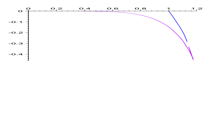
Figure 11: Free energy versus temperature for the near-extremal NS5-branes. Displayed are the non-uniform (blue) and localized (magenta) phases. The uniform phase is located at the point $(T,F)=(T_{\rm hg},0)$.

Before considering the new data for the localized phase, we list the main properties of the three different phases (already stated in [57]) that arise from the corresponding phases of neutral Kaluza-Klein black holes:

• Uniform phase. This phase has zero free energy and a fixed temperature $T=T_{\rm hg}$ and captures the well-known Hagedorn-like behavior of LST. It corresponds to a single point in the free energy versus temperature diagram in Figure 11.

• Non-uniform phase. This phase emerges out of the point $(T,F)=(T_{\rm hg},0)$ and exhibits increasing temperature and decreasing free energy. It has positive specific heat. For temperatures near the Hagedorn temperature $0\leq T-T_{\rm hg}\ll T_{\rm hg}$, one finds

  $$F_{\rm nu}(T)\simeq-2\pi V_{5}N^{3}T_{\rm hg}^{6}\left[1.54\cdot\left(\frac{T}{T_{\rm hg}}-1\right)+3.23\cdot\left(\frac{T}{T_{\rm hg}}-1\right)^{2}\right]\ .$$ (7.14)

  This expression has been computed in [57] using results of [31].

• Localized phase. The localized phase begins at the point $(T,F)=(0,0)$, which corresponds to the $(2,0)$ SCFT, the infrared fixed point of the type IIA near-extremal NS5-brane. The first correction to the thermodynamics as we raise the temperature and move away from the infrared fixed point is [57]

  $$F_{\rm loc}(T)=-\frac{2^{6}\pi^{3}}{3^{7}}V_{5}N^{3}T^{6}\left[1+\frac{2^{5}\zeta(3)}{3^{6}}\frac{T^{6}}{T_{\rm hg}^{6}}+{\cal{O}}\left(\frac{T^{12}}{T_{\rm hg}^{12}}\right)\right]\ .$$ (7.15)

  This has been computed using the results of [39].

One can say more about the localized phase by using the numerical data of [46]. The localized phase begins at the point $(T,F)=(0,0)$ and has decreasing free energy until the maximum temperature $T_{\rm\star}=1.177\cdot T_{\rm hg}$. At this point the curve reverses direction and has decreasing temperature and increasing free energy.

The most intriguing part of the localized phase is evidently the behavior near the maximal temperature $T_{\rm\star}$. One way to understand the behavior around this point is to consider the temperature versus energy diagram in Fig. 12. In this diagram the localized phase is apparently a smooth curve. Hence, the entropy is continuous at $T\simeq T_{\rm\star}$. However, since the temperature is maximal at $T=T_{\rm\star}$ the $(E,T)$ curve has a horizontal tangent at that point. This implies that the localized phase has positive specific heat as $T$ increases from zero to $T_{\rm\star}$ which becomes infinite at the maximal temperature $T_{\rm\star}$. Continuing along the same curve in the $(E,T)$ diagram we begin with minus infinite specific heat and continue with negative specific heat until the curve develops a vertical tangent. At that point the specific heat becomes zero. For the remaining part of the curve the specific heat is positive.

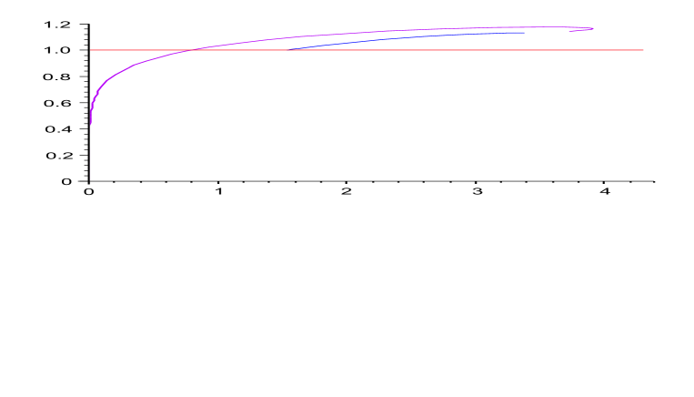
Figure 12: Temperature versus energy for the near-extremal NS5-branes. Displayed are the uniform (red), non-uniform (blue) and localized (magenta) phases.

Let us consider more closely the thermodynamics around the critical temperature $T_{\star}$. From the available data we get

$$T\simeq T_{\star}-c(E-E_{\star})^{2}\ ,\ \ c=0.038\ ,\ \ \frac{E_{\star}}{V_{5}}=3.60\cdot(2\pi)^{-5}l_{s}^{-6}\ .$$ (7.16)

From this expression we can obtain the free energy as a function of temperature near the singularity

$$\begin{array}[]{c}\displaystyle F(T)\simeq F_{\star}-S_{\star}(T-T_{\star})\pm\frac{2}{3\sqrt{c}T_{\star}}(T-T_{\star})^{3/2}\ ,\\[8.53581pt] \displaystyle\frac{S_{\star}}{V_{5}}=3.5\cdot(2\pi)^{-4}\sqrt{N}\ ,\ \ \frac{F_{\star}}{V_{5}}\equiv\frac{1}{V_{5}}(E_{\star}-S_{\star}T_{\star})=-0.53\cdot(2\pi)^{-5}l_{s}^{-6}\ .\end{array}$$ (7.17)

In the first equation the $\pm$ sign corresponds to the two branches on either side of the maximum temperature point. The minus branch is the one that has positive specific heat (for this branch $E\lesssim E_{\star}$) and the plus branch is the one that has negative specific heat (for this branch $E\gtrsim E_{\star}$). It is immediately clear from (7.17) that the entropy is indeed finite and continuous at the critical point, whereas the heat capacity diverges and changes sign.

Also it is clear from Fig. 11 that there are temperatures where more than one phases are available. The dominant phase will be the one with the lowest free energy. It corresponds to the localized phase, which lies within the energy range $0\leq E\leq E_{\star}$. Hence, in the canonical ensemble we conclude that the system is (globally) thermodynamically unstable in the uniform phase (at zero free energy and temperature $T=T_{\rm hg}$) and will decay to the localized solution at the same temperature. In the dominant, localized phase the heat capacity will increase as we increase the temperature and eventually will become infinite at the maximal temparature $T=T_{\rm\star}$. This implies that $T_{\star}$ is a limiting temperature. Note that this limiting temperature exceeds the temperature $T_{\rm hg}$ associated with the uniform phase.

Microcanonical ensemble

We now turn to the microcanonical ensemble. The entropy of the three different phases as a function of energy is displayed in Fig. 13. The main properties of these phases are

• Uniform phase. This phase corresponds to the horizontal line in Fig. 13 and exhibits Hagedorn behavior. The entropy as a function of energy (see (5.29)) is

  $$S_{\rm u}(E)=\frac{E}{T_{\rm hg}}\ .$$ (7.18)

• Non-uniform phase. This phase emerges at the point $(E,S)=(E_{\rm c},S_{\rm c})$, and for energies close to the critical energy $E_{\rm c}$ we have [57]

  $$\frac{S(E)}{S_{u}(E)}\simeq 1-0.05\cdot\left[\frac{(2\pi)^{5}l_{s}^{6}}{V_{5}}(E-E_{\rm c})\right]^{2}\ ,\ \ \frac{E_{\rm c}}{V_{5}}=1.54\cdot(2\pi)^{-5}l_{s}^{-6}\ ,\ \ 0\leq\frac{l_{s}^{6}(E-E_{c})}{V_{5}}\ll 1\ .$$ (7.19)

  This expression has been computed using the results of [31]. The entropy function for the entire non-uniform phase, as displayed in Fig. 13, was computed in [57] using the data of [30].

• Localized phase. The localized phase begins at the origin $(E,S)=(0,0)$. At very low energies we obtain, using the results of [39], the analytical result [57]

  $$S_{\rm loc}(E)\simeq\frac{2\pi^{1/3}}{3}(\frac{6}{5})^{5/6}\frac{\sqrt{N}}{(2\pi)^{4}}\frac{V_{5}}{l_{s}^{5}}\left((2\pi)^{5}\frac{l_{s}^{6}E}{V_{5}}\right)^{5/6}\left(1+\frac{\zeta(3)}{10\pi^{2}}(2\pi)^{5}\frac{l_{s}^{6}E}{V_{5}}\right)\ ,\ \ \frac{l_{s}^{6}E}{V_{5}}\ll 1\ .$$ (7.20)

  The entropy function for the entire localized phase, as displayed in Fig. 13, has been computed using the data of [46] and the map of [57].

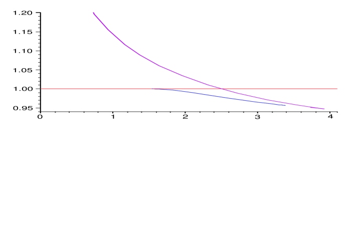
Figure 13: Entropy versus energy for the near-extremal NS5-branes. On the vertical axis we plot the ratio $S(E)/S_{\rm u}(E)$ and on the horizontal axis $E/E_{\rm c}$. $S_{\rm u}(E)$ denotes the entropy function of the uniform phase of near-extremal NS5-branes. Displayed are the uniform (red), non-uniform (blue) and localized (magenta) phases.

In the microcanonical ensemble, the phase with the highest entropy dominates. Hence, from Fig. 13 we conclude that for energies below $E_{\#}/V_{5}=2.51\cdot(2\pi)^{-5}l_{s}^{-6}$, the localized phase is preferred in the canonical ensemble, whereas for energies above that value the system is in the uniform phase. In the range $E_{\#}<E\leq E_{\rm max}$, with $E_{\rm max}/V_{5}=3.92\cdot(2\pi)^{-5}l_{s}^{-6}$, the entropy of the uniform phase is greater than that of the localized phase. For $E>E_{\rm max}$ only the uniform phase is available. Note that $E_{\#}<E_{\star}<E_{\rm max}$. The non-uniform phase has always lower entropy than the other two phases.

The point of the localized phase where $E=E_{\rm max}$ is special. The heat capacity is zero there, which corresponds to a singular behavior in the microcanonical ensemble and prompts the interpretation of the energy $E_{\rm max}$ as a limiting energy for the localized phase. It is also interesting to consider what happens to the system with energy $E<E_{\#}$ when we throw in a finite amount of energy $\Delta E$. There are three possibilities. If $E+\Delta E<E_{\#}$ or $E_{\#}<E+\Delta E<E_{\rm max}$ the system will remain in the localized phase. In the second case, however, the entropy of the uniform phase at the new energy $E+\Delta E$ will be greater so the system will probably go through a phase transition to end up in the uniform phase. Finally, if $E+\Delta E>E_{\rm max}$ the only available phase is the uniform phase and the system presumably has to end up in that phase.

Comparing the ensembles

Comparing the canonical and microcanonical ensembles, we see significant differences in the qualitative behavior of the near-extremal NS5-brane thermodynamics. In the canonical ensemble, the localized phase is always the dominant phase in the interval $E\leq E_{\star}$, and has a positive specific heat and a limiting temperature $T_{\star}$. In the microcanonical ensemble, the localized phase is again the dominant phase for energies $E\leq E_{\#}$. However, the qualitative behavior is very different for energies $E_{\#}<E<E_{\rm max}$. In this energy range the uniform phase is dominant. Hence, we find different preferred phases in the two ensembles. For energies $E>E_{\rm max}$ there is an even more dramatic difference between the two ensembles since the only available phase is the uniform phase in the canonical ensemble. Consequently, it seems that the two ensembles are completely inequivalent at large energies.

Since we discuss a system without gravity one would expect that it is always possible to bring it in contact with a heat bath of a certain temperature. Therefore, the inequivalence of ensembles could suggest a subtlety in the definition of the canonical ensemble. Alternatively, it could point towards the existence of a new hitherto unknown phase of near-extremal NS5-branes. This could potentially resolve the issue arising from the absence of any stable phases with temperatures greater than $T_{\star}$. See the conclusions of Ref. [58] for further discussion on these issues.

7.3 D-brane bound states

In the above discussion we considered the implications of the Gregory-Laflamme instability when there is a singly-charged brane with a compact direction. It is also interesting to consider brane bound state backgrounds without compact directions. In this case the CSC conjecture still applies, as reviewed in Section 6, thus giving a connection between the Gregory-Laflamme instability, the local thermodynamical stability and the stability of the dual non-gravitational theories living on the brane bound states.

In [59] the implications of the Gregory-Laflamme instability for the phase-structure of the non-commutative Yang-Mills (NCYM) theories were described. The dynamics of open strings ending on a D$p$-brane are described at low energies by super-Yang-Mills theory in $p+1$ dimensions. For a D-brane in the presence of an NS-NS B-field the same dynamics is captured by a non-commutative gauge theory [181, 182, 183, 184]. One can then obtain the holographic dual of the NCYM theory by taking the near-horizon limit of $N$ parallel D-branes in the presence of an NS-NS B-field. This implies, in particular, that the near-extremal limit of the thermal D1-D3 brane bound state is holographically dual to a four-dimensional NCYM theory with a non-zero temperature [185, 186, 146, 187, 188]. In [59] it was argued that the D$(p-2)$-D$p$ brane bound state is unstable in the near-extremal limit for all temperatures above zero. This can be seen using the condition (6.23) for thermodynamic stability of the D$(p-2)$-D$p$ brane bound state derived in Section 6.2.

Ref. [61] discussed similar implications for the non-commutative open string (NCOS) theories living on the brane bound states. The effective low energy dynamics of open strings ending on an F1-D$p$ brane bound state are described by a Non-Commutative Open String (NCOS) theory, which is a theory of open strings on a target space in which space and time does not commute [189, 190]. Taking the near-extremal limit of the non-extremal F1-D$p$ bound state we obtain a gravity dual for the $(p+1)$-dimensional NCOS theory [147]. In [61] it was argued that the near-extremal F1-D$p$ bound state is unstable above a certain critical temperature.

Similar considerations also hold for other non-gravitational theories on brane bound states, such as the OM theory on the M2-M5 brane bound state [191, 192] and the ODp-theories on the D$p$-NS5 brane bound state [191, 193].

8 Discussion and outlook

In this review we summarized the current state of knowledge on the classical stability of black branes in pure gravity and supergravity. We focused mainly on the case of static black hole solutions that asymptote to a Kaluza-Klein space of the form ${\cal M}^{d}\times S^{1}$. Although this is the simplest possible case in a large class of solutions that asymptote to Kaluza-Klein spaces of the form ${\cal M}^{d}\times{\cal N}$, where ${\cal N}$ is any compact Ricci flat manifold, we have seen that it exhibits a profoundly rich structure with many features that are expected to be part of the more general story. We would like to conclude with a summary of other known classical instabilities in gravity and a list of important questions that deserve further study.

8.1 Other classical instabilities

Ultra-spin instability

Rotating black holes in higher dimensions with arbitrary angular momentum were discovered twenty years ago by Myers and Perry [14]. The absence of an upper bound on the angular momentum (in six and higher dimensions) should be contrasted with the situation in four dimensions, where the Kerr black hole obeys the famous Kerr bound $J<GM^{2}$, and with the similar bound $J^{2}<32GM^{3}/(27\pi)$ for the five dimensional Myers-Perry black hole. Nevertheless, it was argued in [194] that in six or higher dimensions the Myers-Perry black hole becomes unstable above some critical angular momentum thus recovering a dynamical Kerr bound. The instability was identified as a Gregory-Laflamme instability by showing that in a large angular momentum limit the black hole geometry becomes that of an unstable black membrane. This result is also an indication of the existence of new rotating black holes with spherical topology, where the horizon is distorted by ripples along the polar direction. Furthermore it suggests that a possible endpoint of the decay process in ultra-spinning black holes is the fragmentation of the original black hole into multiple black holes. Ref. [194] verified that this possibility is consistent with a global thermodynamic argument. An alternative conjecture for the evolution of the ultra-spin instability is that the decay proceeds via emission of gravitational radiation. In the process, the black hole sheds a fraction of both its spin and mass and settles down in a range of parameters within the stable regime. Comments on this alternative possibility can also be found in [194].

It should be emphasized that up to date the complete analytic theory of perturbations around the higher-dimensional rotating black holes has not been developed. Progress in this direction has been achieved in special cases (odd number of space-time dimensions, equal angular momenta) in [195].

Although the arguments presented in [194] apply only to six or higher dimensions an instability in five dimensions is also expected [15]. Entropy arguments suggest that in this case the endpoint of the instability is the five dimensional black ring.

Gyration instability

In the context of D1-D5-P spinning black brane solutions in type IIB supergravity compactified on $\mathbb{T}^{4}$ it has been argued in [152] that a small perturbation of a spinning black string could grow to become large for sufficiently large angular momentum. The endpoint of this instability is expected to be a gyrating string where part of the original angular momentum is carried by gyrations of the string (as opposed to spin). This type of instability has been proposed as a possible counterexample to the CSC (see also Section 6.3).

Superradiance instability

Superradiance is a phenomenon that occurs in a scattering process when the incident wave is reflected back amplified. The first classic example of superradiant scattering, which later led to the notion of superradiant scattering in black hole space-times, was given by Zel’dovich in [196, 197]. By examining what happens when scalar waves of the form $e^{-i\omega t+im\phi}$ scatter off a rotating absorbing cylinder, Zel’dovich concluded that the scattered wave is amplified provided that the frequency $\omega$ of the incident wave satisfies the inequality

$$\omega<m\Omega~{}.$$ (8.1)

In this relation $\Omega$ is the angular velocity of the rotating cylinder. Similar superradiant scattering occurs in the background of Kerr black holes [196, 197, 198, 199, 200] for frequencies $\omega$ still satisfying (8.1) with $\Omega$ the angular velocity of the black hole.

An instability can occur if the black hole is surrounded by a reflecting wall that scatters the returning wave back towards the horizon. In that case the wave will bounce back and forth from the horizon extracting an exponentially growing amount of energy from the black hole until the pressure destroys the mirror. The combined system of the black hole and the mirror is known as Press and Teukolsky’s black hole bomb [201, 202]. A natural reflecting wall occurs in a variety of situations: a massive scalar field propagating in a Kerr background [203, 204, 205], a wave propagating around spinning black strings [152, 206, 207], Kerr-anti-deSitter black holes [208], large radius doubly spinning black rings [209]. In general, the unstable modes can be scalar, electromagnetic or gravitational.

Ergoregion instability

Space-times with ergospheres and no horizon are unstable under perturbations of scalar and electromagnetic fields or gravitational waves [210]. The instability also occurs in the case of rotating stars with an ergoregion [211, 212] and in smooth non-supersymmetric D1-D5-P geometries [213]. In the latter case the endpoint of the instability has been argued to be a smooth supersymmetric configuration.

A detour on the stability of black rings

The recent discovery of the black ring solution in five dimensions [15] demonstrates clearly that in higher dimensions new qualitative features can appear which are not present in four dimensions. Most notably, one finds that there are black holes with non-spherical horizon topologies and that conventional notions of black hole uniqueness do not apply. This realization has made the five dimensional black ring a protagonist in the arena of higher dimensional black hole physics. Some important partial results on the classical stability of the five-dimensional black ring have been obtained. Here we review the emerging picture beginning with a quick reminder of the major features of black rings. We will see that black rings can exhibit a combination of the above-mentioned instabilities and more. We will focus mostly on neutral black rings.

The neutral black ring metric has been discussed in a series of papers [15, 216, 115] (for a recent review of the subject with a complete list of references see [217]). The resulting one-parameter family of solutions is conveniently parameterized by a single variable $\nu$ in the range $0<\nu\leq 1$. In terms of $\nu$ the dimensionless angular momentum and horizon area are given by the expressions

$$j^{2}=\frac{27\pi}{32G}\frac{J^{2}}{M^{3}}=\frac{(1+\nu)^{3}}{8\nu}~{},~{}~{}a_{H}=\frac{3}{16}\sqrt{\frac{3}{\pi}}\frac{{\cal A}_{H}}{(GM)^{3/2}}=2\sqrt{\nu(1-\nu)}~{}.$$ (8.2)

Compare these with the corresponding expressions for the five dimensional Myers-Perry black hole

$$j^{2}=\frac{2\nu}{1+\nu}~{},~{}~{}a_{H}=2\sqrt{2\frac{1-\nu}{1+\nu}}~{}.$$ (8.3)

The situation is summarized for fixed mass in Fig. 14 along with the corresponding curve for the Myers-Perry black hole. This diagram has two striking features. First, there is a range of $j$ where three objects with the same mass and spin coexist (one Myers-Perry black hole and two black rings). Secondly, the black ring curve exhibits a cusp at $\nu=\frac{1}{2}$ which is the meeting point of two branches of black rings. One branch has $0<\nu<1/2$ and has been called the branch of thin black rings, because it includes the regime $\nu\sim 0$ of very thin (highly spinning) rings. The other branch with $1/2<\nu<1$ has been called the branch of fat black rings and terminates at the singular solution with $\nu=1$.

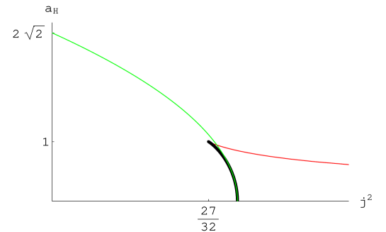
Figure 14: Rescaled horizon area $a_{H}$ versus angular momentum squared $j^{2}$ for five-dimensional Myers-Perry black holes and black rings. The green curve represents the Myers-Perry black hole, the red curve (for $\nu>\frac{1}{2}$) the branch of fat black rings and the solid black curve (for $0<\nu<\frac{1}{2}$) the branch of thin black rings.

The classical stability of these solutions has been studied with a combination of methods (qualitative and semi-quantitative) in [15, 218, 219, 220, 221, 116, 222, 223] and has led to the following picture (this picture has been recently summarized and further elaborated upon in [223] to which we refer the interested reader for more details):

• At large angular momentum the thin black ring becomes identical to a highly boosted black string (see Section 4.2) which is known to exhibit a Gregory-Laflamme instability. This suggests [15, 116] that the thin black ring branch suffers from a Gregory-Laflamme instability quite possibly driving the system towards a configuration of two or more spinning black holes. There are some similarities here with the case of ultra-spinning Myers-Perry black holes in six or higher dimensions.

• Black rings can become unstable under radial perturbations. The analysis of [116] indicates that fat black rings are radially unstable while thin black rings are radially stable. The black ring with minimal spin is also argued to be unstable. This type of instability appears to mesh nicely with the topological arguments of [218, 219] which are based on the Poincaré method.

• The angular momentum of black rings is bounded from below. By absorbing a counter-spinning null-particle the black ring can decrease its angular momentum $j$. For the lowest-spinning black ring this process indicates an instability. On the other hand, it is impossible for a Myers-Perry black hole or a fat black ring to overspin by absorbing a co-rotating null particle or to spontaneously decay by emitting null particles without violating the area law [223].

• Doubly spinning large radius ($i.e.$ $\nu\rightarrow 0$) thin black rings have been argued to suffer from superradiance instabilities [209].

The addition of charges can improve the stability of black rings. For instance, supersymmetric black rings [224] are expected to be stable. Black rings with dipole charges [115] are expected to suffer from similar instabilities as the neutral ones [223].

8.2 Future directions and open problems

We conclude with a number of important issues and questions for future research.

Pure gravity: static solutions asymptoting to ${\cal M}^{d}\times S^{1}$

• At present the complete non-uniform branch is known numerically for $d=4$ and $d=5$ [30, 32] and recently also higher dimensions $6\leq d\leq 10$ have been studied [33]. It would be interesting to compute it above the critical dimension, $i.e.$ $d\geq 13$. For the black hole branch, the present status is that we know numerically the entire branch only for $d=4$ and $d=5$ [44, 45, 46]. Having the numerical data for other dimensions would be interesting as well.

• If possible, it would be interesting to find the analytic form of the non-uniform and black hole branches, for example using the ansatz (3.11). A first step in this direction would be to extend the known first order analytical results to second order. For the $d=4$ black hole this has been done in Ref. [42], while [43] gives the corrected thermodynamics for all $d$, but not the metric.

• For the neutral black string the study of the classical stability revealed the presence of the GL instability. It would be highly interesting if one could study the classical stability of other branches of solutions, such as the non-uniform black string, the localized black hole, or a black hole attached to a Kaluza-Klein bubble.

• The bubble-black hole sequences are only known in five and six dimensions. It is interesting to ask if solutions for bubble-black hole sequences exist for $D\geq 7$, and if so, whether they can be related to the solutions of [50] by a map similar to the one mapping five- to six-dimensional solutions. For spaces with more than one Kaluza-Klein circle, $i.e.$ asymptotics ${\cal M}^{d}\times\mathbb{T}^{k\geq 2}$, it is easy to construct solutions describing regular bubble-black hole sequences [50]. On the other hand, finding bubble-black hole sequences in ${\cal M}^{d}\times S^{1}$ may be difficult since one cannot use the generalized Weyl ansatz for such solutions, but we do not see any physical obstructions to their existence. Should these higher dimensional bubble-black hole sequences exist, it would be interesting to see what type of horizon topologies they exhibit.

• In connection with the above points, also the general question of the $d$-dependence of the phase diagram is an important one. For example, the non-uniform branch is known to have a critical dimension beyond which the slope changes sign. Likewise one could imagine new phases appearing (or other phases disappearing) as the number of dimensions increases.

• The instability of the uniform black string implies that a naked singularity may be formed when the horizon of the black string pinches off. As originally pointed out by Gregory and Laflamme [2, 3], this would entail a violation of the Cosmic Censorship Hypothesis. The results of [30, 46, 32, 33] suggest that, for certain dimensions, the localized black hole is the only solution with higher entropy than that of the uniform black string (for masses where the black string is unstable). Thus, the endpoint of the instability seems to be the localized black hole which means that the horizon should pinch off in the classical evolution. On the other hand, in [17] it was argued that the horizon cannot pinch off in finite affine parameter, thus suggesting that it is impossible for the black string horizon to pinch off. A way to reconcile these two results is if the horizon pinches off in infinite affine parameter (see also [73]). Recently, the numerical analysis of [74, 75, 76] indicates that this indeed is the case. If this is correct it would be interesting to examine the implications for the Cosmic Censorship Hypothesis.

• A similar formation of a naked singularity (now for static configurations) has been predicted at the merger point of the non-uniform and localized black hole branch in the phase diagram of black strings. Direct evidence for the existence of the merger point has been found with a numerical study in [52] (see also [34, 27]). It would be very interesting to explore the physics of the merger point transition further.

Pure gravity: static solutions asymptoting to ${\cal M}^{d}\times{\cal N}$

Static solutions in pure gravity asymptoting to ${\cal M}^{d}\times S^{1}$ exhibit a rich structure. An even richer structure is expected for static solutions asymptoting to the more general manifold ${\cal M}^{d}\times{\cal N}$ where ${\cal N}$ is any compact Ricci-flat manifold. It would be interesting to explore the ${\cal N}$ dependence of the phase structure of solutions in certain examples, $e.g.$ with ${\cal N}$ being an $n$-torus $\mathbb{T}^{n}$ or ${\cal N}$ being a Calabi-Yau manifold. Uniformly smeared solutions are still expected on general grounds to exhibit Gregory-Laflamme instabilities, but it would be further interesting to see if the phase diagram of the general case exhibits new qualitative features which are not present in the simplest ${\cal N}=S^{1}$ case. A recent discussion of the Gregory-Laflamme instability for ${\cal N}=\mathbb{T}^{n}$ appeared in [37]. For some preliminary comments on the case of a general compact Ricci flat manifold ${\cal N}$ see Section 4.3.

Static black brane solutions in supergravity

Many of the above pure gravity neutral static solutions can be easily lifted to corresponding solutions in type IIA or type IIB ten-dimensional supergravity where one can also make contact with D-brane configurations and gauge theories. It would be interesting to explore the full phase diagram of static solutions in ten-dimensional supergravity independently and see whether it admits new phases which cannot be obtained through a map from the neutral pure gravity ones. In this connection, we note that in Ref. [141] a new stable phase of non-uniform black strings was found.

Black hole microscopics

Another interesting direction is to make contact with microscopic calculations of the entropy of black holes. While this is difficult for neutral Kaluza-Klein black holes, charging up the solutions by the boost/U-duality map and taking the near-extremal limit opens up the possibility of applying microscopic conjectures. This was successfully applied in Ref. [77] where five-dimensional three-charge black holes on a a circle were obtained by extending the map of Ref. [57] to include three charges. As a result a rich phase structure of three-charge black holes, including a new phase of three-charge black holes that are non-uniformly distributed on the circle, was found via a map that relates them to the phases of five-dimensional neutral Kaluza-Klein black holes. Moreover, for three-charge black holes localized on the transverse circle, it was shown that in a partial extremal limit with two charges sent to infinity and one finite, the first correction to the finite entropy is in agreement with the microscopic entropy. This was achieved by taking into account that the number of branes shift as a consequence of the interactions across the transverse circle. This matching was extended in Ref. [78] to second order. Furthermore, in Ref. [78] a simple microscopic model was proposed that reproduces most of the features of the phase diagram, including the new non-uniform phase. It would be interesting to pursue this microscopic description further (in this connection see e.g. the reviews [225, 226]).

Connection to thermodynamics

A natural and intuitive connection between classical and thermodynamic instabilities of black brane solutions is expected to hold in general. The conjecture underlying this relation (Correlated Stability Conjecture) has passed a large number of tests, but is known to fail in certain cases as we saw in section 6. It would be interesting to formulate a refinement of the conjecture that survives all known tests. Then one could hope to find a general proof for its validity.

Other compactified solutions

It would also be interesting to examine the existence of other classes of solutions with a compactified direction. For example in Ref. [227] a supersymmetric rotating black hole in a compactified space-time was found and charged black holes in compactified space-times are considered in Ref. [228]. In another direction, new solutions with Kaluza-Klein boundary conditions for anti-de-Sitter space times have recently been constructed in Refs. [229, 230].

Black rings

For black rings in five dimensions (and for that matter also for other higher dimensional black holes like the rotating Myers-Perry solutions) it is important to develop further the explicit linear stability analysis. The main obstacle in this enterprize is of course the complexity of the equations in higher dimensions. The ultimate goal in that respect is a better understanding of the full phase diagram. Beyond that it would be very exciting to see if there are black ring solutions in $D>5$ dimensions or other solutions with the more complex horizon topology allowed by topological arguments in higher dimensions [214, 215].

Braneworld black holes

The higher dimensional black holes and branes described in this review appear naturally in the discussion of the braneworld model of large extra dimensions [53, 54]. In other braneworld models such as the one proposed by Randall and Sundrum [231, 232] the geometry is warped in the extra direction and the discovery of black hole solutions in this context has proven more difficult. A black string solution is also allowed in this model and is expected to have a Gregory-Laflamme instability as in the case of uniform black strings in KK space-times. Localized black hole solutions are anticipated as end-products of the Gregory-Laflamme instability of black strings, but have not been constructed explicitly so far. A partial list of references includes [233, 234, 235, 236] (see also the recent work in [237, 238] and references therein). It should be noted that exact black hole solutions localized on the four-dimensional braneworld have been constructed by the authors of [239, 240].

Appendix A The Gregory-Laflamme mode

In this appendix we consider in more detail the Gregory-Laflamme mode [2, 3] for the metric (2.9) that describes a uniform black string in $D=d+1$ dimensions. The instability mode is given by a metric perturbation $h_{\mu\nu}$ that solves the perturbed Einstein equations of motion around the black string metric (2.9). The precise form of the perturbation $h_{\mu\nu}$ appears in the main text in eqs. (2.11) and (2.12). In (2.12) $\psi$, $\eta$, $\chi$ and $\kappa$ are all functions of the variable

$$x=\frac{rk}{r_{0}}\ ,$$ (A.1)

and this will be the variable with respect to which we take derivatives. The function $f$ is given in terms of $x$ as

$$f=1-\frac{k^{d-3}}{x^{d-3}}\ .$$ (A.2)

Following [89, 151, 35] we work here in a transverse $(\nabla^{\mu}h_{\mu\nu}=0)$, traceless $(g^{\mu\nu}h_{\mu\nu}=0)$ gauge. The tracelessness condition is

$$(d-2)\kappa+\chi+\psi=0\ .$$ (A.3)

The transversality conditions are

$$\begin{array}[]{c}\displaystyle\frac{\Omega}{k}x\psi+(d-3)(1-f)\eta+f\left((d-2)\eta+x\eta^{\prime}\right)=0\ ,\\[8.53581pt] \displaystyle-2\frac{\Omega}{k}x\eta+(d-3)(1-f)(\chi-\psi)+2f\left((d-1)\chi+\psi+x\chi^{\prime}\right)=0\ .\end{array}$$ (A.4)

The four independent Einstein equations take the form

$$\displaystyle\begin{array}[]{l}\displaystyle x\frac{\Omega}{k}\psi+(d-3)(1-f)\eta+\frac{k}{\Omega}f^{2}\big{(}(d-2)\psi^{\prime}+x\psi^{\prime\prime}\big{)}\\[5.69054pt] \displaystyle+f\left[2(d-2)\eta-x\frac{k}{\Omega}\psi+2x\eta^{\prime}+\frac{k}{\Omega}(d-3)(1-f)(-\chi^{\prime}+\psi^{\prime})\right]=0~{},\end{array}$$ (A.7)

$$\displaystyle-(d-3)(1-f)x\frac{\Omega}{k}(\chi+\psi)+2f\left[x\frac{\Omega}{k}((d-1)\chi+\psi+x(\chi^{\prime}+\psi^{\prime}))+\eta x^{2}\right]=0~{},~{}~{}$$ (A.8)

$$\displaystyle\begin{array}[]{l}\displaystyle x^{2}\bigg{(}\frac{\Omega^{2}}{k^{2}}+f\bigg{)}\chi-(d-3)(1-f)\frac{\Omega}{k}x\eta\\[11.38109pt] \displaystyle+f\left[-2x^{2}\frac{\Omega}{k}\eta^{\prime}+(d-3)(1-f)x(\chi^{\prime}-\psi^{\prime})+xf\big{(}d\chi^{\prime}+2\psi^{\prime}+x\chi^{\prime\prime}\big{)}\right]=0~{},\end{array}$$ (A.11)

$$\displaystyle\begin{array}[]{l}f\bigg{[}\psi\big{(}-x^{2}+2(d-3)(1-f)\big{)}+\chi\big{(}-x^{2}+2(d-1)(d-3)(1-f)\big{)}\\ \displaystyle-2(d-2)x\frac{\Omega}{k}\eta+(d-3)(1-f)x(\chi^{\prime}+\psi^{\prime})\bigg{]}+f^{2}\bigg{[}2(d-1)(d-3)\chi\\ \displaystyle+2(d-3)\psi+x\big{(}3(d-2)\chi^{\prime}+(d-2)\psi^{\prime}+x(\chi^{\prime\prime}+\psi^{\prime\prime})\big{)}\bigg{]}-x^{2}\frac{\Omega^{2}}{k^{2}}(\chi+\psi)=0~{}.\end{array}$$ (A.15)

Combining the gauge conditions (A.3)-(A.4) with the Einstein equations (A.7)-(A.15) one can derive Eq. (2.13) which is a second order differential equation for $\psi$ of the form

$$\psi^{\prime\prime}(x)+{\cal Q}_{d}(x)\psi^{\prime}(x)+{\cal P}_{d}(x)\psi(x)=0~{}.$$ (A.16)

${\cal Q}_{d}$ and ${\cal P}_{d}$ are $d$-dependent rational functions of $x$, which we summarize here for completeness

$${\cal Q}_{d}(x) = f^{-1}x^{-1}\Big{[}f^{3}k^{4}(39+10d+3d^{2})+\Omega^{2}\big{(}k^{2}(3-d)^{2}-4\Omega^{2}\big{)}$$ (A.17)

$$+k^{2}f^{2}\big{(}-2k^{2}(41-16d+d^{2})-3(d+5)(5-3d)\Omega^{2}\big{)}$$

$$-k^{2}f\big{(}k^{2}(3-d)^{2}+2(-5-12d+5d^{2})\Omega^{2}\big{)}\Big{]}^{-1}$$

$$\times\Big{[}k^{4}f^{4}(36+11d+6d^{2}-d^{3})-3(3-d)\Omega^{2}\big{(}k^{2}(3-d)^{2}-4\Omega^{2}\big{)}$$

$$+k^{2}f^{2}\big{(}k^{2}(3-d)(64-23d+d^{2})+\Omega^{2}(-431+405d-181d^{2}+31d^{3})\big{)}$$

$$+k^{2}f^{3}\big{(}k^{2}(-178+28d-2d^{2}+4d^{3})+\Omega^{2}(135-94d+51d^{2}-8d^{3})\big{)}$$

$$f\big{(}2k^{4}(3-d)^{3}+k^{2}\Omega^{2}(3-d)(163-127d+26d^{2})+4(-7+2d)\Omega^{4}\big{)}\Big{]}~{},$$

$${\cal P}_{d}(x) = k^{-2}f^{-2}x^{-2}\Big{[}f^{3}k^{4}(39+10d+3d^{2})+\Omega^{2}\big{(}k^{2}(3-d)^{2}-4\Omega^{2}\big{)}$$ (A.18)

$$+k^{2}f^{2}\big{(}-2k^{2}(41-16d+d^{2})-3(5+d)(5-3d)\Omega^{2}\big{)}$$

$$-k^{2}f\big{(}k^{2}(3-d)^{2}+2(-5-12d+5d^{2})\Omega^{2}\big{)}\Big{]}^{-1}\times\Big{[}-2k^{6}f^{5}(1-d)^{2}(3-d)^{2}$$

$$+k^{4}f^{4}\big{(}2k^{2}(-3+d)(-16+21d-11d^{2}+2d^{3})+(-39-10d-3d^{2})x^{2})$$

$$-(3-d)^{2}(1-d)(37-7d)\Omega^{2}\big{)}$$

$$-2k^{4}f^{3}\big{(}k^{2}((-3+d)(-25+21d-7d^{2}+d^{3})+(-41+16d-d^{2})x^{2})$$

$$+((3-d)(-239+273d-91d^{2}+9d^{3})+(-21+18d+7d^{2})x^{2})\Omega^{2}\big{)}$$

$$+2fk^{2}\Omega^{2}\big{(}k^{2}(3-d)^{2}(35-14d+d^{2}+x^{2})$$

$$+(2(3-d)(d-2)+(57-56d+13d^{2})x^{2})\Omega^{2}\big{)}$$

$$+\Omega^{2}\big{(}k^{4}(3-d)^{4}-k^{2}(3-d)^{2}(-2+7x^{2})\Omega^{2}+4x^{2}\Omega^{4}\big{)}$$

$$+k^{2}f^{2}\big{(}k^{4}(3-d)^{2}(8-2d+x^{2})-2k^{2}((-3+d)(-302+279d-80d^{2}+7d^{3})$$

$$-6(d-2)^{2}x^{2})\Omega^{2}+(2(d-3)(d-1)+(9+22d-19d^{2})x^{2})\Omega^{4}\big{)}\Big{]}~{}.$$

The threshold unstable mode obeys the differential equation (A.16) with $\Omega=0$, which is equivalent to the second order equation for the scalar $\chi$ that appears in (2.10) of [35]

$$-f\chi^{\prime\prime} + \left[\frac{2x^{2}(ff^{\prime\prime}-f^{\prime 2})-x(d-2)ff^{\prime}+2df^{2}}{x(xf^{\prime}-2f)}\right]\chi^{\prime}$$ (A.19)

$$+ \left[\frac{x^{2}f^{\prime}f^{\prime\prime}+x\left[2(d-1)ff^{\prime\prime}-(d+2){f^{\prime}}^{2}\right]+4ff^{\prime}}{x(xf^{\prime}-2f)}\right]\chi=-r_{0}^{2}\chi~{}.$$

The differential equations governing the threshold unstable mode have appeared in the literature in various forms depending on the choice of gauge. A complete list of the gauge choices that have been employed so far in the literature can be found in appendix A of [87]. Differential equations for the general time-dependent Gregory-Laflamme mode have appeared also in [2] (see eq. 10, which is a second order differential equation for $h^{tr}$) and in [56] (see eq. 12).

References

- [1] J. H. Jeans, “The stability of a spherical nebula,” Phil. Trans. Roy. Soc. 199A (1902) 1–53.
- [2] R. Gregory and R. Laflamme, “Black strings and -branes are unstable,” Phys. Rev. Lett. 70 (1993) 2837–2840, hep-th/9301052.
- [3] R. Gregory and R. Laflamme, “The instability of charged black strings and -branes,” Nucl. Phys. B428 (1994) 399–434, hep-th/9404071.
- [4] T. Regge, “Stability of a Schwarzschild singularity,” Phys. Rev. 108 (1957) 1063–1069.
- [5] F. J. Zerilli, “Gravitational field of a particle falling in a Schwarzschild geometry analyzed in tensor harmonics,” Phys. Rev. D2 (1970) 2141–2160.
- [6] W. Israel, “Event horizons in static vacuum space-times,” Phys. Rev. 164 (1967) 1776–1779.
- [7] B. Carter, “Axisymmetric black hole has only two degrees of freedom,” Phys. Rev. Lett. 26 (1971) 331–333.
- [8] S. W. Hawking, “Black holes in General Relativity,” Commun. Math. Phys. 25 (1972) 152–166.
- [9] D. C. Robinson, “Uniqueness of the Kerr black hole,” Phys. Rev. Lett. 34 (1975) 905–906.
- [10] G. W. Gibbons, D. Ida, and T. Shiromizu, “Uniqueness and non-uniqueness of static vacuum black holes in higher dimensions,” Prog. Theor. Phys. Suppl. 148 (2003) 284–290, gr-qc/0203004.
- [11] G. W. Gibbons, D. Ida, and T. Shiromizu, “Uniqueness and non-uniqueness of static black holes in higher dimensions,” Phys. Rev. Lett. 89 (2002) 041101, hep-th/0206049.
- [12] F. R. Tangherlini, “Schwarzschild field in n dimensions and the dimensionality of space problem,” Nuovo Cimento 27 (1963) 636.
- [13] S. Hollands, A. Ishibashi, and R. M. Wald, “A higher dimensional stationary rotating black hole must be axisymmetric,” Commun. Math. Phys. 271 (2007) 699–722, gr-qc/0605106.
- [14] R. C. Myers and M. J. Perry, “Black holes in higher dimensional space-times,” Ann. Phys. 172 (1986) 304.
- [15] R. Emparan and H. S. Reall, “A rotating black ring in five dimensions,” Phys. Rev. Lett. 88 (2002) 101101, hep-th/0110260.
- [16] B. Kol, “Speculative generalization of black hole uniqueness to higher dimensions,” hep-th/0208056.
- [17] G. T. Horowitz and K. Maeda, “Fate of the black string instability,” Phys. Rev. Lett. 87 (2001) 131301, hep-th/0105111.
- [18] G. T. Horowitz, “Playing with black strings,” hep-th/0205069.
- [19] J. M. Maldacena, “The large limit of superconformal field theories and supergravity,” Adv. Theor. Math. Phys. 2 (1998) 231–252, hep-th/9711200.
- [20] S. S. Gubser, I. R. Klebanov, and A. M. Polyakov, “Gauge theory correlators from noncritical string theory,” Phys. Lett. B428 (1998) 105, hep-th/9802109.
- [21] E. Witten, “Anti-de Sitter space and holography,” Adv. Theor. Math. Phys. 2 (1998) 253, hep-th/9802150.
- [22] N. Itzhaki, J. M. Maldacena, J. Sonnenschein, and S. Yankielowicz, “Supergravity and the large limit of theories with sixteen supercharges,” Phys. Rev. D58 (1998) 046004, hep-th/9802042.
- [23] A. Sen, “Tachyon dynamics in open string theory,” Int. J. Mod. Phys. A20 (2005) 5513–5656, hep-th/0410103.
- [24] M. Headrick, S. Minwalla, and T. Takayanagi, “Closed string tachyon condensation: An overview,” Class. Quant. Grav. 21 (2004) S1539–S1565, hep-th/0405064.
- [25] D. Kutasov and N. Seiberg, “Number of degrees of freedom, density of states and tachyons in string theory and CFT,” Nucl. Phys. B358 (1991) 600–618.
- [26] V. Niarchos, “Density of states and tachyons in open and closed string theory,” JHEP 06 (2001) 048, hep-th/0010154.
- [27] B. Kol, “The phase transition between caged black holes and black strings: A review,” Phys. Rept. 422 (2006) 119–165, hep-th/0411240.
- [28] R. Gregory and R. Laflamme, “Hypercylindrical black holes,” Phys. Rev. D37 (1988) 305.
- [29] S. S. Gubser, “On non-uniform black branes,” Class. Quant. Grav. 19 (2002) 4825–4844, hep-th/0110193.
- [30] T. Wiseman, “Static axisymmetric vacuum solutions and non-uniform black strings,” Class. Quant. Grav. 20 (2003) 1137–1176, hep-th/0209051.
- [31] E. Sorkin, “A critical dimension in the black-string phase transition,” Phys. Rev. Lett. 93 (2004) 031601, hep-th/0402216.
- [32] B. Kleihaus, J. Kunz, and E. Radu, “New nonuniform black string solutions,” JHEP 06 (2006) 016, hep-th/0603119.
- [33] E. Sorkin, “Non-uniform black strings in various dimensions,” Phys. Rev. D74 (2006) 104027, gr-qc/0608115.
- [34] B. Kol, “Topology change in general relativity and the black-hole black-string transition,” hep-th/0206220.
- [35] B. Kol and E. Sorkin, “On black-brane instability in an arbitrary dimension,” Class. Quant. Grav. 21 (2004) 4793–4804, gr-qc/0407058.
- [36] V. Cardoso and O. J. C. Dias, “Rayleigh-Plateau and Gregory-Laflamme instabilities of black strings,” Phys. Rev. Lett. 96 (2006) 181601, hep-th/0602017.
- [37] B. Kol and E. Sorkin, “LG (Landau-Ginzburg) in GL (Gregory-Laflamme),” Class. Quant. Grav. 23 (2006) 4563–4592, hep-th/0604015.
- [38] T. Harmark and N. A. Obers, “Black holes on cylinders,” JHEP 05 (2002) 032, hep-th/0204047.
- [39] T. Harmark, “Small black holes on cylinders,” Phys. Rev. D69 (2004) 104015, hep-th/0310259.
- [40] D. Gorbonos and B. Kol, “A dialogue of multipoles: Matched asymptotic expansion for caged black holes,” JHEP 06 (2004) 053, hep-th/0406002.
- [41] D. Gorbonos and B. Kol, “Matched asymptotic expansion for caged black holes: Regularization of the post-Newtonian order,” Class. Quant. Grav. 22 (2005) 3935–3960, hep-th/0505009.
- [42] D. Karasik, C. Sahabandu, P. Suranyi, and L. C. R. Wijewardhana, “Analytic approximation to 5 dimensional black holes with one compact dimension,” Phys. Rev. D71 (2005) 024024, hep-th/0410078.
- [43] Y.-Z. Chu, W. D. Goldberger, and I. Z. Rothstein, “Asymptotics of -dimensional Kaluza-Klein black holes: Beyond the Newtonian approximation,” JHEP 03 (2006) 013, hep-th/0602016.
- [44] E. Sorkin, B. Kol, and T. Piran, “Caged black holes: Black holes in compactified spacetimes. II: 5d numerical implementation,” Phys. Rev. D69 (2004) 064032, hep-th/0310096.
- [45] H. Kudoh and T. Wiseman, “Properties of Kaluza-Klein black holes,” Prog. Theor. Phys. 111 (2004) 475–507, hep-th/0310104.
- [46] H. Kudoh and T. Wiseman, “Connecting black holes and black strings,” Phys. Rev. Lett. 94 (2005) 161102, hep-th/0409111.
- [47] T. Harmark and N. A. Obers, “New phase diagram for black holes and strings on cylinders,” Class. Quantum Grav. 21 (2004) 1709–1724, hep-th/0309116.
- [48] B. Kol, E. Sorkin, and T. Piran, “Caged black holes: Black holes in compactified spacetimes. I: Theory,” Phys. Rev. D69 (2004) 064031, hep-th/0309190.
- [49] T. Harmark and N. A. Obers, “Phase structure of black holes and strings on cylinders,” Nucl. Phys. B684 (2004) 183–208, hep-th/0309230.
- [50] H. Elvang, T. Harmark, and N. A. Obers, “Sequences of bubbles and holes: New phases of Kaluza-Klein black holes,” JHEP 01 (2005) 003, hep-th/0407050.
- [51] T. Wiseman, “From black strings to black holes,” Class. Quant. Grav. 20 (2003) 1177–1186, hep-th/0211028.
- [52] B. Kol and T. Wiseman, “Evidence that highly non-uniform black strings have a conical waist,” Class. Quant. Grav. 20 (2003) 3493–3504, hep-th/0304070.
- [53] N. Arkani-Hamed, S. Dimopoulos, and G. R. Dvali, “The hierarchy problem and new dimensions at a millimeter,” Phys. Lett. B429 (1998) 263–272, hep-ph/9803315.
- [54] I. Antoniadis, N. Arkani-Hamed, S. Dimopoulos, and G. R. Dvali, “New dimensions at a millimeter to a Fermi and superstrings at a TeV,” Phys. Lett. B436 (1998) 257–263, hep-ph/9804398.
- [55] P. Bostock and S. F. Ross, “Smeared branes and the Gubser-Mitra conjecture,” Phys. Rev. D70 (2004) 064014, hep-th/0405026.
- [56] O. Aharony, J. Marsano, S. Minwalla, and T. Wiseman, “Black hole - black string phase transitions in thermal 1+1 dimensional supersymmetric Yang-Mills theory on a circle,” Class. Quant. Grav. 21 (2004) 5169–5192, hep-th/0406210.
- [57] T. Harmark and N. A. Obers, “New phases of near-extremal branes on a circle,” JHEP 09 (2004) 022, hep-th/0407094.
- [58] T. Harmark and N. A. Obers, “Thermodynamics of the near-extremal NS5-brane,” Nucl. Phys. B742 (2006) 41–58, hep-th/0510098.
- [59] S. S. Gubser, “The Gregory-Laflamme instability for the D2-D0 bound state,” JHEP 02 (2005) 040, hep-th/0411257.
- [60] S. F. Ross and T. Wiseman, “Smeared D0 charge and the Gubser-Mitra conjecture,” Class. Quant. Grav. 22 (2005) 2933–2946, hep-th/0503152.
- [61] J. J. Friess and S. S. Gubser, “Instabilities of D-brane bound states and their related theories,” JHEP 11 (2005) 040, hep-th/0503193.
- [62] S. S. Gubser and I. Mitra, “Instability of charged black holes in anti-de Sitter space,” hep-th/0009126.
- [63] S. S. Gubser and I. Mitra, “The evolution of unstable black holes in anti-de Sitter space,” JHEP 08 (2001) 018, hep-th/0011127.
- [64] H. S. Reall, “Classical and thermodynamic stability of black branes,” Phys. Rev. D64 (2001) 044005, hep-th/0104071.
- [65] J. P. Gregory and S. F. Ross, “Stability and the negative mode for Schwarzschild in a finite cavity,” Phys. Rev. D64 (2001) 124006, hep-th/0106220.
- [66] T. Harmark, V. Niarchos, and N. A. Obers, “Instabilities of near-extremal smeared branes and the correlated stability conjecture,” JHEP 10 (2005) 045, hep-th/0509011.
- [67] J. J. Friess, S. S. Gubser, and I. Mitra, “Counter-examples to the correlated stability conjecture,” Phys. Rev. D72 (2005) 104019, hep-th/0508220.
- [68] B. Kol, “Choptuik scaling and the merger transition,” JHEP 10 (2006) 017, hep-th/0502033.
- [69] E. Sorkin and Y. Oren, “On Choptuik’s scaling in higher dimensions,” Phys. Rev. D71 (2005) 124005, hep-th/0502034.
- [70] V. P. Frolov, “Merger transitions in brane-black-hole systems: Criticality, scaling, and self-similarity,” Phys. Rev. D74 (2006) 044006, gr-qc/0604114.
- [71] V. Asnin, B. Kol, and M. Smolkin, “Analytic evidence for continuous self similarity of the critical merger solution,” Class. Quant. Grav. 23 (2006) 6805–6827, hep-th/0607129.
- [72] M. W. Choptuik, “Universality and scaling in gravitational collapse of a massless scalar field,” Phys. Rev. Lett. 70 (1993) 9–12.
- [73] D. Marolf, “On the fate of black string instabilities: An observation,” Phys. Rev. D71 (2005) 127504, hep-th/0504045.
- [74] M. W. Choptuik et al., “Towards the final fate of an unstable black string,” Phys. Rev. D68 (2003) 044001, gr-qc/0304085.
- [75] D. Garfinkle, L. Lehner, and F. Pretorius, “A numerical examination of an evolving black string horizon,” Phys. Rev. D71 (2005) 064009, gr-qc/0412014.
- [76] M. Anderson, L. Lehner, and J. Pullin, “Arbitrary black-string deformations in the black string - black hole transitions,” Phys. Rev. D73 (2006) 064011, hep-th/0510051.
- [77] T. Harmark, K. R. Kristjansson, N. A. Obers, and P. B. Ronne, “Three-charge black holes on a circle,” hep-th/0606246. To appear in JHEP.
- [78] B. D. Chowdhury, S. Giusto, and S. D. Mathur, “A microscopic model for the black hole - black string phase transition,” Nucl. Phys. B762 (2007) 301–343, hep-th/0610069.
- [79] S. W. Hawking and D. N. Page, “Thermodynamics of black holes in Anti-de Sitter space,” Commun. Math. Phys. 87 (1983) 577.
- [80] E. Witten, “Anti-de Sitter space, thermal phase transition, and confinement in gauge theories,” Adv. Theor. Math. Phys. 2 (1998) 505, hep-th/9803131.
- [81] B. Sundborg, “The Hagedorn transition, deconfinement and SYM theory,” Nucl. Phys. B573 (2000) 349–363, hep-th/9908001.
- [82] O. Aharony, J. Marsano, S. Minwalla, K. Papadodimas, and M. Van Raamsdonk, “The Hagedorn/deconfinement phase transition in weakly coupled large gauge theories,” Adv. Theor. Math. Phys. 8 (2004) 603–696, hep-th/0310285.
- [83] O. Aharony, J. Marsano, S. Minwalla, K. Papadodimas, and M. Van Raamsdonk, “A first order deconfinement transition in large Yang- Mills theory on a small ,” Phys. Rev. D71 (2005) 125018, hep-th/0502149.
- [84] H. Kodama and A. Ishibashi, “A master equation for gravitational perturbations of maximally symmetric black holes in higher dimensions,” Prog. Theor. Phys. 110 (2003) 701–722, hep-th/0305147.
- [85] A. Ishibashi and H. Kodama, “Stability of higher-dimensional Schwarzschild black holes,” Prog. Theor. Phys. 110 (2003) 901–919, hep-th/0305185.
- [86] H. Kodama and A. Ishibashi, “Master equations for perturbations of generalized static black holes with charge in higher dimensions,” Prog. Theor. Phys. 111 (2004) 29–73, hep-th/0308128.
- [87] B. Kol, “The power of action: ’The’ derivation of the black hole negative mode,” hep-th/0608001.
- [88] B. Kol, “Perturbations around backgrounds with one non-homogeneous dimension,” hep-th/0609001.
- [89] D. J. Gross, M. J. Perry, and L. G. Yaffe, “Instability of flat space at finite temperature,” Phys. Rev. D25 (1982) 330–355.
- [90] E. Witten, “Instability of the Kaluza-Klein vacuum,” Nucl. Phys. B195 (1982) 481.
- [91] O. Sarbach and L. Lehner, “Critical bubbles and implications for critical black strings,” Phys. Rev. D71 (2005) 026002, hep-th/0407265.
- [92] D. Brill and G. T. Horowitz, “Negative energy in string theory,” Phys. Lett. B262 (1991) 437–443.
- [93] S. Corley and T. Jacobson, “Collapse of Kaluza-Klein bubbles,” Phys. Rev. D49 (1994) 6261–6263, gr-qc/9403017.
- [94] O. Sarbach and L. Lehner, “No naked singularities in homogeneous, spherically symmetric bubble spacetimes,” Phys. Rev. D69 (2004) 021901, hep-th/0308116.
- [95] G. T. Horowitz, “Tachyon condensation and black strings,” JHEP 08 (2005) 091, hep-th/0506166.
- [96] T. Harmark and N. A. Obers, “Phases of Kaluza-Klein black holes: A brief review,” hep-th/0503020.
- [97] T. Harmark and N. A. Obers, “General definition of gravitational tension,” JHEP 05 (2004) 043, hep-th/0403103.
- [98] S. W. Hawking and G. T. Horowitz, “The gravitational Hamiltonian, action, entropy and surface terms,” Class. Quant. Grav. 13 (1996) 1487–1498, gr-qc/9501014.
- [99] R. C. Myers, “Stress tensors and Casimir energies in the AdS/CFT correspondence,” Phys. Rev. D60 (1999) 046002, hep-th/9903203.
- [100] J. H. Traschen and D. Fox, “Tension perturbations of black brane spacetimes,” Class. Quant. Grav. 21 (2004) 289–306, gr-qc/0103106.
- [101] P. K. Townsend and M. Zamaklar, “The first law of black brane mechanics,” Class. Quant. Grav. 18 (2001) 5269–5286, hep-th/0107228.
- [102] J. H. Traschen, “A positivity theorem for gravitational tension in brane spacetimes,” Class. Quant. Grav. 21 (2004) 1343–1350, hep-th/0308173.
- [103] T. Shiromizu, D. Ida, and S. Tomizawa, “Kinematical bound in asymptotically translationally invariant spacetimes,” Phys. Rev. D69 (2004) 027503, gr-qc/0309061.
- [104] D. Kastor and J. Traschen, “Stresses and strains in the first law for Kaluza-Klein black holes,” JHEP 09 (2006) 022, hep-th/0607051.
- [105] O. J. C. Dias, T. Harmark, R. C. Myers, and N. A. Obers, “Multi-black hole configurations on the cylinder,” arXiv:0706.3645 [hep-th].
- [106] T. Harmark and N. A. Obers, “Black holes and black strings on cylinders,” Fortsch. Phys. 51 (2003) 793–798, hep-th/0301020.
- [107] R. C. Myers, “Higher dimensional black holes in compactified space- times,” Phys. Rev. D35 (1987) 455.
- [108] A. R. Bogojevic and L. Perivolaropoulos, “Black holes in a periodic universe,” Mod. Phys. Lett. A6 (1991) 369–376.
- [109] D. Korotkin and H. Nicolai, “A periodic analog of the Schwarzschild solution,” gr-qc/9403029.
- [110] A. V. Frolov and V. P. Frolov, “Black holes in a compactified spacetime,” Phys. Rev. D67 (2003) 124025, hep-th/0302085.
- [111] P.-J. De Smet, “Black holes on cylinders are not algebraically special,” Class. Quant. Grav. 19 (2002) 4877–4896, hep-th/0206106.
- [112] R. Emparan and H. S. Reall, “Generalized Weyl solutions,” Phys. Rev. D65 (2002) 084025, hep-th/0110258.
- [113] T. Harmark, “Stationary and axisymmetric solutions of higher-dimensional general relativity,” Phys. Rev. D70 (2004) 124002, hep-th/0408141.
- [114] H. Elvang and G. T. Horowitz, “When black holes meet Kaluza-Klein bubbles,” Phys. Rev. D67 (2003) 044015, hep-th/0210303.
- [115] R. Emparan, “Rotating circular strings, and infinite non-uniqueness of black rings,” JHEP 03 (2004) 064, hep-th/0402149.
- [116] J. L. Hovdebo and R. C. Myers, “Black rings, boosted strings and Gregory-Laflamme,” Phys. Rev. D73 (2006) 084013, hep-th/0601079.
- [117] M.-I. Park, “The final state of black strings and -branes, and the Gregory-Laflamme instability,” Class. Quant. Grav. 22 (2005) 2607–2614, hep-th/0405045.
- [118] S. Ferrara, R. Kallosh, and A. Strominger, “N=2 extremal black holes,” Phys. Rev. D52 (1995) 5412–5416, hep-th/9508072.
- [119] D. Kastor and K. Z. Win, “Non-extreme Calabi-Yau black holes,” Phys. Lett. B411 (1997) 33–38, hep-th/9705090.
- [120] B. Pioline, “Lectures on on black holes, topological strings and quantum attractors,” Class. Quant. Grav. 23 (2006) S981, hep-th/0607227.
- [121] L. Landau and E. M. Lifshitz, “Statistical physics,” Course of theoretical Physics Vol. 9 (1980).
- [122] H. Kudoh and U. Miyamoto, “On non-uniform smeared black branes,” Class. Quant. Grav. 22 (2005) 3853–3874, hep-th/0506019.
- [123] J. Milnor, “Morse theory,” Annals of Mathematics Studies No. 51 (Princeton University Press, 1963).
- [124] D. J. Gross and E. Witten, “Possible third order phase transition in the large lattice gauge theory,” Phys. Rev. D21 (1980) 446–453.
- [125] B. R. Greene, “String theory on Calabi-Yau manifolds,” hep-th/9702155.
- [126] E. Thorne, K. S., E. Price, R. H., and E. Macdonald, D. A., “Black holes: The membrane paradigm,”. New Haven, USA: Yale Univ. pr. (1986) 367p.
- [127] P. Kovtun, D. T. Son, and A. O. Starinets, “Holography and hydrodynamics: Diffusion on stretched horizons,” JHEP 10 (2003) 064, hep-th/0309213.
- [128] P. Kovtun, D. T. Son, and A. O. Starinets, “Viscosity in strongly interacting quantum field theories from black hole physics,” Phys. Rev. Lett. 94 (2005) 111601, hep-th/0405231.
- [129] V. Cardoso and L. Gualtieri, “Equilibrium configurations of fluids and their stability in higher dimensions,” Class. Quant. Grav. 23 (2006) 7151–7198, hep-th/0610004.
- [130] H. Kudoh, “Origin of black string instability,” Phys. Rev. D73 (2006) 104034, hep-th/0602001.
- [131] R. Gregory and R. Laflamme, “Evidence for stability of extremal black -branes,” Phys. Rev. D51 (1995) 305–309, hep-th/9410050.
- [132] R. Gregory, “Black string instabilities in anti-de Sitter space,” Class. Quant. Grav. 17 (2000) L125–L132, hep-th/0004101.
- [133] T. Hirayama and G. Kang, “Stable black strings in anti-de Sitter space,” Phys. Rev. D64 (2001) 064010, hep-th/0104213.
- [134] V. E. Hubeny and M. Rangamani, “Unstable horizons,” JHEP 05 (2002) 027, hep-th/0202189.
- [135] T. Hirayama, G.-w. Kang, and Y.-o. Lee, “Classical stability of charged black branes and the Gubser-Mitra conjecture,” Phys. Rev. D67 (2003) 024007, hep-th/0209181.
- [136] S. S. Gubser and A. Ozakin, “Universality classes for horizon instabilities,” JHEP 05 (2003) 010, hep-th/0301002.
- [137] S. A. Hartnoll, “Instability of generalised AdS black holes and thermal field theory,” JHEP 08 (2003) 019, hep-th/0305001.
- [138] G. Kang and J. Lee, “Classical stability of black D3-branes,” JHEP 03 (2004) 039, hep-th/0401225.
- [139] G. Kang, “Classical stability of black branes,” J. Korean Phys. Soc. 45 (2004) S86–S89, hep-th/0403015.
- [140] G. Kang and Y. Lee, “Stability of smeared black branes and the Gubser-Mitra conjecture,” hep-th/0504031.
- [141] U. Miyamoto and H. Kudoh, “New stable phase of non-uniform charged black strings,” JHEP 12 (2006) 048, gr-qc/0609046.
- [142] N. A. Obers and B. Pioline, “U-duality and M-theory,” Phys. Rept. 318 (1999) 113–225, hep-th/9809039.
- [143] T. Harmark, K. R. Kristjansson, N. A. Obers, and P. B. Ronne, Work in progress.
- [144] G. T. Horowitz and K. Maeda, “Inhomogeneous near-extremal black branes,” Phys. Rev. D65 (2002) 104028, hep-th/0201241.
- [145] T. Harmark and N. A. Obers, “Thermodynamics of spinning branes and their dual field theories,” JHEP 01 (2000) 008, hep-th/9910036.
- [146] T. Harmark and N. A. Obers, “Phase structure of non-commutative field theories and spinning brane bound states,” JHEP 03 (2000) 024, hep-th/9911169.
- [147] T. Harmark, “Supergravity and space-time non-commutative open string theory,” JHEP 07 (2000) 043, hep-th/0006023.
- [148] I. Y. Aref’eva, M. G. Ivanov, and I. V. Volovich, “Non-extremal intersecting -branes in various dimensions,” Phys. Lett. B406 (1997) 44–48, hep-th/9702079.
- [149] A. Buchel, “A holographic perspective on Gubser-Mitra conjecture,” Nucl. Phys. B731 (2005) 109–124, hep-th/0507275.
- [150] B. F. Whiting and J. York, James W., “Action principle and partition function for the gravitational field in black hole topologies,” Phys. Rev. Lett. 61 (1988) 1336.
- [151] T. Prestidge, “Dynamic and thermodynamic stability and negative modes in Schwarzschild-anti-de Sitter,” Phys. Rev. D61 (2000) 084002, hep-th/9907163.
- [152] D. Marolf and B. C. Palmer, “Gyrating strings: A new instability of black strings?,” Phys. Rev. D70 (2004) 084045, hep-th/0404139.
- [153] G. T. Horowitz and D. Marolf, “Counting states of black strings with traveling waves. II,” Phys. Rev. D55 (1997) 846–852, hep-th/9606113.
- [154] O. Aharony, S. S. Gubser, J. Maldacena, H. Ooguri, and Y. Oz, “Large field theories, string theory and gravity,” Phys. Rept. 323 (2000) 183, hep-th/9905111.
- [155] T. Harmark and N. A. Obers, “New phases of thermal SYM and LST from Kaluza-Klein black holes,” Fortsch. Phys. 53 (2005) 536–541, hep-th/0503021.
- [156] L. Susskind, “Matrix theory black holes and the Gross-Witten transition,” hep-th/9805115.
- [157] J. L. F. Barbon, I. I. Kogan, and E. Rabinovici, “On stringy thresholds in SYM/AdS thermodynamics,” Nucl. Phys. B544 (1999) 104, hep-th/9809033.
- [158] M. Li, E. J. Martinec, and V. Sahakian, “Black holes and the SYM phase diagram,” Phys. Rev. D59 (1999) 044035, hep-th/9809061.
- [159] E. J. Martinec and V. Sahakian, “Black holes and the SYM phase diagram. II,” Phys. Rev. D59 (1999) 124005, hep-th/9810224.
- [160] E. J. Martinec, “Black holes and the phases of brane thermodynamics,” hep-th/9909049.
- [161] L. Fidkowski and S. Shenker, “D-brane instability as a large phase transition,” hep-th/0406086.
- [162] T. Hollowood, S. P. Kumar, and A. Naqvi, “Instabilities of the small black hole: A view from ,” JHEP 01 (2007) 001, hep-th/0607111.
- [163] O. Aharony et al., “The phase structure of low dimensional large gauge theories on tori,” JHEP 01 (2006) 140, hep-th/0508077.
- [164] J. M. Maldacena and A. Strominger, “Semiclassical decay of near-extremal fivebranes,” JHEP 12 (1997) 008, hep-th/9710014.
- [165] O. Aharony, M. Berkooz, D. Kutasov, and N. Seiberg, “Linear dilatons, NS5-branes and holography,” JHEP 10 (1998) 004, hep-th/9808149.
- [166] M. Berkooz, M. Rozali, and N. Seiberg, “Matrix description of M theory on and ,” Phys. Lett. B408 (1997) 105–110, hep-th/9704089.
- [167] N. Seiberg, “New theories in six-dimensions and matrix description of M theory on and ,” Phys. Lett. B408 (1997) 98–104, hep-th/9705221.
- [168] R. Dijkgraaf, E. Verlinde, and H. Verlinde, “Notes on matrix and micro strings,” Nucl. Phys. Proc. Suppl. 62 (1998) 348, hep-th/9709107.
- [169] O. Aharony, “A brief review of ’little string theories’,” Class. Quant. Grav. 17 (2000) 929, hep-th/9911147.
- [170] D. Kutasov, “Introduction to little string theory,”. Prepared for ICTP Spring School on Superstrings and Related Matters, Trieste, Italy, 2-10 Apr 2001.
- [171] J. M. Maldacena, “Statistical entropy of near extremal five-branes,” Nucl. Phys. B477 (1996) 168–174, hep-th/9605016.
- [172] T. Harmark and N. A. Obers, “Hagedorn behaviour of little string theory from string corrections to NS5-branes,” Phys. Lett. B485 (2000) 285, hep-th/0005021.
- [173] M. Berkooz and M. Rozali, “Near Hagedorn dynamics of NS fivebranes, or a new universality class of coiled strings,” JHEP 05 (2000) 040, hep-th/0005047.
- [174] D. Kutasov and D. A. Sahakyan, “Comments on the thermodynamics of little string theory,” JHEP 02 (2001) 021, hep-th/0012258.
- [175] M. Rangamani, “Little string thermodynamics,” JHEP 06 (2001) 042, hep-th/0104125.
- [176] A. Buchel, “On the thermodynamic instability of LST,” hep-th/0107102.
- [177] K. Narayan and M. Rangamani, “Hot little string correlators: A view from supergravity,” JHEP 08 (2001) 054, hep-th/0107111.
- [178] P. A. DeBoer and M. Rozali, “Thermal correlators in little string theory,” Phys. Rev. D67 (2003) 086009, hep-th/0301059.
- [179] O. Aharony, A. Giveon, and D. Kutasov, “LSZ in LST,” Nucl. Phys. B691 (2004) 3–78, hep-th/0404016.
- [180] A. Parnachev and A. Starinets, “The silence of the little strings,” JHEP 10 (2005) 027, hep-th/0506144.
- [181] A. Connes, M. R. Douglas, and A. S. Schwarz, “Noncommutative geometry and matrix theory: Compactification on tori,” JHEP 02 (1998) 003, hep-th/9711162.
- [182] M. R. Douglas and C. M. Hull, “D-branes and the noncommutative torus,” JHEP 02 (1998) 008, hep-th/9711165.
- [183] Y.-K. E. Cheung and M. Krogh, “Noncommutative geometry from 0-branes in a background B- field,” Nucl. Phys. B528 (1998) 185, hep-th/9803031.
- [184] N. Seiberg and E. Witten, “String theory and noncommutative geometry,” JHEP 09 (1999) 032, hep-th/9908142.
- [185] J. M. Maldacena and J. G. Russo, “Large limit of non-commutative gauge theories,” JHEP 09 (1999) 025, hep-th/9908134.
- [186] M. Alishahiha, Y. Oz, and M. M. Sheikh-Jabbari, “Supergravity and large noncommutative field theories,” JHEP 11 (1999) 007, hep-th/9909215.
- [187] R.-G. Cai and N. Ohta, “On the thermodynamics of large non-commutative super Yang-Mills theory,” Phys. Rev. D61 (2000) 124012, hep-th/9910092.
- [188] R.-G. Cai and N. Ohta, “Noncommutative and ordinary super Yang–Mills on (D, D) bound states,” JHEP 03 (2000) 009, hep-th/0001213.
- [189] N. Seiberg, L. Susskind, and N. Toumbas, “Strings in background electric field, space/time noncommutativity and a new noncritical string theory,” JHEP 06 (2000) 021, hep-th/0005040.
- [190] R. Gopakumar, J. Maldacena, S. Minwalla, and A. Strominger, “S-duality and noncommutative gauge theory,” JHEP 06 (2000) 036, hep-th/0005048.
- [191] R. Gopakumar, S. Minwalla, N. Seiberg, and A. Strominger, “OM theory in diverse dimensions,” JHEP 08 (2000) 008, hep-th/0006062.
- [192] E. Bergshoeff, D. S. Berman, J. P. van der Schaar, and P. Sundell, “Critical fields on the M5-brane and noncommutative open strings,” Phys. Lett. B492 (2000) 193–200, hep-th/0006112.
- [193] T. Harmark, “Open branes in space-time non-commutative little string theory,” Nucl. Phys. B593 (2001) 76–98, hep-th/0007147.
- [194] R. Emparan and R. C. Myers, “Instability of ultra-spinning black holes,” JHEP 09 (2003) 025, hep-th/0308056.
- [195] H. K. Kunduri, J. Lucietti, and H. S. Reall, “Gravitational perturbations of higher dimensional rotating black holes: Tensor perturbations,” Phys. Rev. D74 (2006) 084021, hep-th/0606076.
- [196] Y. B. Zel’dovich JETP Lett 14 (1971) 180.
- [197] Y. B. Zel’dovich Sov. Phys. JETP 35 (1972) 1085.
- [198] J. M. Bardeen, W. H. Press, and S. A. Teukolsky, “Rotating black holes: Locally nonrotating frames, energy extraction, and scalar synchrotron radiation,” Astrophys. J. 178 (1972) 347.
- [199] A. A. Starobinsky Sov. Phys. JETP 37 (1973) 28.
- [200] A. A. Starobinsky and S. M. Churilov Sov. Phys. JETP 38 (1973) 1.
- [201] W. H. Press and S. A. Teukolsky, “Floating orbits, super-radiant scattering and the black hole bomb,” Nature 238 (1972) 211.
- [202] V. Cardoso, O. J. C. Dias, J. P. S. Lemos, and S. Yoshida, “The black hole bomb and superradiant instabilities,” Phys. Rev. D70 (2004) 044039, hep-th/0404096.
- [203] T. Damour, N. Deruelle, and R. Ruffini, “On quantum resonances in stationary geometries,” Lett. Nuovo Cim. 15 (1976) 257–262.
- [204] S. Detweiler, “Klein-Gordon equation and rotating black holes,” Phys. Rev. D22 (1980) 2323–2326.
- [205] H. Furuhashi and Y. Nambu, “Instability of massive scalar fields in Kerr-Newman spacetime,” Prog. Theor. Phys. 112 (2004) 983–995, gr-qc/0402037.
- [206] V. Cardoso and J. P. S. Lemos, “New instability for rotating black branes and strings,” Phys. Lett. B621 (2005) 219–223, hep-th/0412078.
- [207] V. Cardoso and S. Yoshida, “Superradiant instabilities of rotating black branes and strings,” JHEP 07 (2005) 009, hep-th/0502206.
- [208] V. Cardoso and O. J. C. Dias, “Small Kerr-anti-de Sitter black holes are unstable,” Phys. Rev. D70 (2004) 084011, hep-th/0405006.
- [209] O. J. C. Dias, “Superradiant instability of large radius doubly spinning black rings,” Phys. Rev. D73 (2006) 124035, hep-th/0602064.
- [210] J. L. Friedman, “Ergosphere instability,” Commun. Math. Phys. 63 (1978) 243.
- [211] N. Comins and B. Schutz, “On the ergoregion instability,” Proc. R. Soc. Lond. A 364 (1978) 211.
- [212] S. Yoshida and E. Eriguchi, “Ergoregion instability revisited - a new and general method for numerical analysis of stability,” MNRAS 282 (1996) 580.
- [213] V. Cardoso, O. J. C. Dias, J. L. Hovdebo, and R. C. Myers, “Instability of non-supersymmetric smooth geometries,” Phys. Rev. D73 (2006) 064031, hep-th/0512277.
- [214] C. Helfgott, Y. Oz, and Y. Yanay, “On the topology of black hole event horizons in higher dimensions,” JHEP 02 (2006) 025, hep-th/0509013.
- [215] G. J. Galloway and R. Schoen, “A generalization of Hawking’s black hole topology theorem to higher dimensions,” Commun. Math. Phys. 266 (2006) 571–576, gr-qc/0509107.
- [216] H. Elvang and R. Emparan, “Black rings, supertubes, and a stringy resolution of black hole non-uniqueness,” JHEP 11 (2003) 035, hep-th/0310008.
- [217] R. Emparan and H. S. Reall, “Black rings,” Class. Quant. Grav. 23 (2006) R169, hep-th/0608012.
- [218] G. Arcioni and E. Lozano-Tellechea, “Stability and critical phenomena of black holes and black rings,” Phys. Rev. D72 (2005) 104021, hep-th/0412118.
- [219] G. Arcioni and E. Lozano-Tellechea, “Stability and thermodynamics of black rings,” hep-th/0502121.
- [220] M. Nozawa and K.-i. Maeda, “Energy extraction from higher dimensional black holes and black rings,” Phys. Rev. D71 (2005) 084028, hep-th/0502166.
- [221] V. Cardoso, O. J. C. Dias, and S. Yoshida, “Perturbations and absorption cross-section of infinite- radius black rings,” Phys. Rev. D72 (2005) 024025, hep-th/0505209.
- [222] D. Astefanesei and E. Radu, “Quasilocal formalism and black ring thermodynamics,” Phys. Rev. D73 (2006) 044014, hep-th/0509144.
- [223] H. Elvang, R. Emparan, and A. Virmani, “Dynamics and stability of black rings,” JHEP 12 (2006) 074, hep-th/0608076.
- [224] H. Elvang, R. Emparan, D. Mateos, and H. S. Reall, “A supersymmetric black ring,” Phys. Rev. Lett. 93 (2004) 211302, hep-th/0407065.
- [225] S. D. Mathur, “The fuzzball proposal for black holes: An elementary review,” Fortsch. Phys. 53 (2005) 793–827, hep-th/0502050.
- [226] S. D. Mathur, “The quantum structure of black holes,” Class. Quant. Grav. 23 (2006) R115, hep-th/0510180.
- [227] K.-i. Maeda, N. Ohta, and M. Tanabe, “A supersymmetric rotating black hole in a compactified spacetime,” Phys. Rev. D74 (2006) 104002, hep-th/0607084.
- [228] M. Karlovini and R. von Unge, “Charged black holes in compactified spacetimes,” Phys. Rev. D72 (2005) 104013, gr-qc/0506073.
- [229] K. Copsey and G. T. Horowitz, “Gravity dual of gauge theory on ,” JHEP 06 (2006) 021, hep-th/0602003.
- [230] R. B. Mann, E. Radu, and C. Stelea, “Black string solutions with negative cosmological constant,” JHEP 09 (2006) 073, hep-th/0604205.
- [231] L. Randall and R. Sundrum, “A large mass hierarchy from a small extra dimension,” Phys. Rev. Lett. 83 (1999) 3370–3373, hep-ph/9905221.
- [232] L. Randall and R. Sundrum, “An alternative to compactification,” Phys. Rev. Lett. 83 (1999) 4690–4693, hep-th/9906064.
- [233] T. Wiseman, “Relativistic stars in Randall-Sundrum gravity,” Phys. Rev. D65 (2002) 124007, hep-th/0111057.
- [234] D. Karasik, C. Sahabandu, P. Suranyi, and L. C. R. Wijewardhana, “Small (1-TeV) black holes in Randall-Sundrum I scenario,” Phys. Rev. D69 (2004) 064022, gr-qc/0309076.
- [235] H. Kudoh, T. Tanaka, and T. Nakamura, “Small localized black holes in braneworld: Formulation and numerical method,” Phys. Rev. D68 (2003) 024035, gr-qc/0301089.
- [236] H. Kudoh, “Thermodynamical properties of small localized black hole,” Prog. Theor. Phys. 110 (2004) 1059–1069, hep-th/0306067.
- [237] S. Creek, R. Gregory, P. Kanti, and B. Mistry, “Braneworld stars and black holes,” Class. Quant. Grav. 23 (2006) 6633–6658, hep-th/0606006.
- [238] A. L. Fitzpatrick, L. Randall, and T. Wiseman, “On the existence and dynamics of braneworld black holes,” JHEP 11 (2006) 033, hep-th/0608208.
- [239] R. Emparan, G. T. Horowitz, and R. C. Myers, “Exact description of black holes on branes,” JHEP 01 (2000) 007, hep-th/9911043.
- [240] R. Emparan, G. T. Horowitz, and R. C. Myers, “Exact description of black holes on branes. II: Comparison with BTZ black holes and black strings,” JHEP 01 (2000) 021, hep-th/9912135.