A String-Inspired Quintom Model Of Dark Energy

Abstract

We propose in this paper a quintom model of dark energy with a single scalar field $\phi$ given by the lagrangian ${\cal L}=-V(\phi)\sqrt{1-\alpha^{\prime}\nabla_{\mu}\phi\nabla^{\mu}\phi+\beta^{\prime}\phi\Box\phi}$. In the limit of $\beta^{\prime}\rightarrow$0 our model reduces to the effective low energy lagrangian of tachyon considered in the literature. We study the cosmological evolution of this model, and show explicitly the behaviors of the equation of state crossing the cosmological constant boundary.

I Introduction

The current data from type Ia supernovae, cosmic microwave background (CMB) radiation, and other cosmological observations[1, 3, 2, 4] have provided strong evidences for a spatially flat and accelerated expanding universe at the present time. Within the framework of the standard cosmology, this acceleration can be understood by introducing a mysterious component, dubbed dark energy (DE). The simplest candidate for DE is a minor positive cosmological constant, but it suffers from the fine-tuning and coincidence problems. As a possible solution to these problems various dynamical models of DE have been proposed, such as quintessence. In the recent years with the accumulated astronomical observational data it becomes possible to probe the current and even early behavior of DE. Although the current fits to the data in combination of the 3-year WMAP[5], the recently released 182 SNIa Gold sample[6] and also other cosmological observational data show the consistence of the cosmological constant, it is worth noting that the dynamical DE models are not excluded and a class of dynamical models with equation of state across $-1$, dubbed quintom, is mildly favored (for recent references see e.g. [7, 8]).

Theoretically it is a big challenge to the model building of the quintom dark energy. The Ref.[9] is the first paper pointing out this challenge and showing explicitly the difficulty of realizing $w$ crossing over $-1$ in the quintessence and phantom like models. In general with a single fluid or a single scalar field with a lagrangian of form ${\cal L}={\cal L}(\phi,\partial_{\mu}\phi\partial^{\mu}\phi)$ it has been proved [10] (see also [9] and [11]) that the dark energy perturbation would be divergent as the equation of state (EOS) $w$ approaches to $-1$. This “no-go” theorem forbids the dynamical models widely studied in the literature with a single scalar field such as quintessence, phantom and k-essence to make the EOS cross over the cosmological constant boundary. The quintom scenario of dark energy is designed to understand the nature of dark energy with $w$ across $-1$. The quintom models of dark energy differ from the quintessence, phantom and k-essence and so on in the determination of the cosmological evolution and the fate of the universe.

To realize a viable quintom scenario of dark energy it needs to introduce extra degree of freedom to the conventional theory with a single fluid or a single scalar field. The first model of quintom scenario of dark energy is given in Ref.[9] with two scalar fields. This model has been studied in detail later on. In the recent years there have been active studies on models of quintom like dark energy such as models with high derivative term[12], vector field[13], or even extended theory of gravity[14] and so on, see e.g. [15].

In this paper, we propose a new type of quintom model inspired by the string theory. We will demonstrate in this paper our model can realize the equation of state crossing $-1$ naturally. This paper is organized as follows. In section 2 we present our model and study its properties especially on the conditions required for the model parameters when $w$ crosses over $-1$. By solving numerically the model we will study the evolution of the equation of state. Moreover, we study the stability property of this model by investigating the quadratic perturbations. The section 3 is the summary of our paper.

II Our Model

Our model is given by the following action

$$S=\int d^{4}x\sqrt{-g}\left[-V(\phi)\sqrt{1-{\alpha}^{\prime}\nabla_{\mu}\phi\nabla^{\mu}\phi+{\beta}^{\prime}\phi\Box\phi}\right].$$ (1)

This model generalizes the usual“Born-Infeld-type” action for the effective description of tachyon dynamics by adding a term $\phi\Box\phi$ to the usual $\nabla_{\mu}\phi\nabla^{\mu}\phi$ in the square root. It is known that the 4D effective action of tachyon dynamics to the lowest order in $\nabla_{\mu}\phi\nabla^{\mu}\phi$ around the top of the tachyon potential can be obtained by the stringy computations for either a D3 brane in bosonic theory [16, 17] or a non-BPS D3 brane in supersymmetric theory [18]. To this order, we have no need to include the operator $\phi\Box\phi$ in the action since it is equivalent to the usual $\nabla_{\mu}\phi\nabla^{\mu}\phi$ term. However, we cannot exclude its existence in an action such as the “Born-Infeld-type” one when incorporating an infinite number of higher derivative terms since now the two terms are in general different dynamically. For example, we cannot simply replace the $\phi\Box\phi$ term in the action (1) by the $\nabla_{\mu}\phi\nabla^{\mu}\phi$. Further this term in the above generalized action has new cosmological consequence as will be shown in this paper. Including an infinite number of higher derivative terms that has a significant cosmological consequence has also been discussed in the context of p-adic string recently in [19]. The two parameters $\alpha^{\prime}$ and $\beta^{\prime}$ in (1) can also be made arbitrary when the background flux is turned on [20]. Without further reasoning, we will take the action (1) as our starting point of phenomenological study.

As will be demonstrated, the $\beta^{\prime}$ term in (1) is crucial to realize the $w$ across $-1$. There we have defined $\alpha^{\prime}=\alpha/M^{4}$ and $\beta^{\prime}=\beta/M^{4}$ with $\alpha$ and $\beta$ being the dimensionless parameters respectively, and $M$ an energy scale used to make the “kinetic energy terms” dimensionless. $V(\phi)$ is the potential of scalar field $\phi$ (e.g., a tachyon) with dimension of ${\rm[mass]}^{4}$ with an expected tachyon potential behavior in general, i.e., bounded and reaching its minimum asymptotically, unless specifically stated. Note that, $\Box=\frac{1}{\sqrt{-g}}\partial_{\mu}\sqrt{-g}g^{\mu\nu}\partial_{\nu}$, therefore, in (1) the terms $\nabla_{\mu}\phi\nabla^{\mu}\phi$ and $\phi\Box\phi$ both involve two fields and two derivatives.

The model with operator $\phi\Box\phi$ for the realization of $w$ crossing $-1$ has been proposed in [12]. However in general for a model with lagrangian as a sum of operators with a polynomial function of the scalar field $\phi$ and its derivatives, the operator $\phi\Box\phi$ can be rewritten as a total derivative term which makes no contribution after integration and a term which renormalizes the canonical kinetic term as discussed above. So if one considers a renormalizable lagrangian, the operator $\phi\Box\phi$ will not be included. Ref.[12] considered a dimension-6 operator as $(\Box\phi)^{2}$. However in the present model, the operator $\phi\Box\phi$ appears at the same order as the operator $\nabla_{\mu}\phi\nabla^{\mu}\phi$ does in the “Born-Infeld-type” action. As discussed above, this model appears more natural than the one used in [12].

With (1) we obtain the equation of motion of the scalar field $\phi$,

$$\frac{\beta}{2}\Box(\frac{V\phi}{f})+\alpha\nabla_{\mu}(\frac{V\nabla^{\mu}\phi}{f})+M^{4}V_{\phi}f+\frac{\beta V}{2f}\Box\phi=0~{},$$ (2)

where $f=\sqrt{1-{\alpha}^{\prime}\nabla_{\mu}\phi\nabla^{\mu}\phi+{\beta}^{\prime}\phi\Box\phi}$ and $V_{\phi}=dV/d\phi$. Following the convention in Ref.[12], the energy-momentum tensor $T^{\mu\nu}$ is given by the standard definition: $\delta_{g_{\mu\nu}}S\equiv-\int d^{4}x\frac{\sqrt{-g}}{2}T^{\mu\nu}\delta g_{\mu\nu}$,

$$T^{\mu\nu} = g^{\mu\nu}[V(\phi)f+\nabla_{\rho}(\psi\nabla^{\rho}\phi)]+\frac{\alpha}{M^{4}}\frac{V(\phi)}{f}\nabla^{\mu}\phi\nabla^{\nu}\phi-\nabla^{\mu}\psi\nabla^{\nu}\phi-\nabla^{\nu}\psi\nabla^{\mu}\phi~{},$$ (3)

where $\psi\equiv\frac{\partial{\cal L}}{\partial\Box\phi}=-\frac{V\beta\phi}{2M^{4}f}$.

For a flat Friedmann-Robertson-Walker (FRW) universe and a homogenous scalar field $\phi$, the equation of motion in (2) can be solved equivalently by the following two equations

$$\ddot{\phi}+3H\dot{\phi} = \frac{\beta V^{2}\phi}{4M^{4}\psi^{2}}-\frac{M^{4}}{\beta\phi}+\frac{\alpha}{\beta\phi}\dot{\phi}^{2}~{},$$ (4)

$$\ddot{\psi}+3H\dot{\psi} = (2\alpha+\beta)(\frac{M^{4}\psi}{\beta^{2}\phi^{2}}-\frac{V^{2}}{4M^{4}\psi})-(2\alpha-\beta)\frac{\alpha\psi}{\beta^{2}\phi^{2}}\dot{\phi}^{2}-\frac{2\alpha}{\beta\phi}\dot{\psi}\dot{\phi}-\frac{\beta V\phi}{2M^{4}\psi}V_{\phi}~{},$$ (5)

where we have made use of the $\psi$ as defined before and the first equation above is just the defining equation for $\psi$ in terms of $\phi$ and its derivatives. $H=\dot{a}/a$ is the Hubble parameter.

One can see from equations above the $\beta$ term plays a role in determining the evolution of the scalar field $\phi$. We can read the energy density from (3) as

$$\rho=Vf+\frac{d}{a^{3}dt}(a^{3}\psi\dot{\phi})+\frac{\alpha}{M^{4}}\frac{V(\phi)}{f}\dot{\phi}^{2}-2\dot{\psi}\dot{\phi}~{},$$ (6)

and similarly the pressure

$$p=-Vf-\frac{d}{a^{3}dt}(a^{3}\psi\dot{\phi})~{}.$$ (7)

With the Friedman equations $H^{2}=\frac{8\pi G}{3}\rho$ and $\dot{H}=-4\pi G(\rho+p)$, we now study the cosmological evolution of equation of state for the present model. Given $w=p/\rho$, we have $\rho+p=(1+w)\rho$. To explore the possibility of the $w$ across $-1$, we need to check if $\frac{d}{dt}(\rho+p)\neq 0$ can be held when $w\rightarrow-1$.

Using (6) and (7) as well as making use of the defining equation for $\psi$, we have

$$\rho+p=\frac{\alpha V(\phi)\dot{\phi}^{2}}{M^{4}f}+\beta\dot{\phi}\frac{d}{dt}[\frac{\phi V(\phi)}{M^{4}f}]~{},$$ (8)

and from which,

$$\frac{d}{dt}(\rho+p) = \frac{\alpha}{M^{4}f^{2}}\{f\frac{d}{dt}[V(\phi)\dot{\phi}^{2}]-\frac{df}{dt}[\dot{\phi}^{2}{V}(\phi)]\}+\beta\ddot{\phi}\frac{d}{dt}[\frac{\phi V(\phi)}{M^{4}f}]+\beta\dot{\phi}\frac{d^{2}}{dt^{2}}[\frac{\phi V(\phi)}{M^{4}f}]~{}.$$ (9)

Eq. (8) implies that we have either (i)$\dot{\phi}=0$ or (ii)$-\frac{\alpha V(\phi)}{f}\dot{\phi}=\beta\frac{d}{dt}[\frac{\phi V(\phi)}{f}]$ when $w\rightarrow-1$.

Let us assume $\dot{\phi}=0$ first when $w\to-1$. With this and Eq. (9), we have $\frac{d}{dt}(\rho+p)=\beta\ddot{\phi}\frac{d}{dt}[\frac{\phi V(\phi)}{M^{4}f}]=-\frac{V(\phi)}{2M^{8}f^{3}}\beta^{2}\phi^{2}\ddot{\phi}\frac{d}{dt}\Box\phi$. Therefore the conditions for having the $w$ across over $-1$ are (i-1)$\phi\neq 0$; (i-2)$\ddot{\phi}\neq 0$; (i-3)$\frac{d}{dt}\Box\phi\neq 0$ in addition to the $\dot{\phi}=0$. Since the characteristic behavior of $V(\phi)$ is to have a finite maximum value at a finite $\phi$ and to reach its (exponentially) vanishing minimum asymptotically where one expects $\ddot{\phi}=0$ and $\frac{d}{dt}\Box\phi=0$ but a non-zero $\dot{\phi}$, so realizing the above crossing over conditions must happen before reaching the potential minimum asymptotically. This implies once the crossing over conditions are met, the field $\phi$ must continue to run away as it should be since we have $\ddot{\phi}\neq 0$.

Let us turn to the second case (ii) when $w\to-1$. We now have $-\frac{\alpha V\dot{\phi}}{f}=\beta\frac{d}{dt}(\frac{\phi V}{f})=\beta\dot{\phi}(\frac{V}{f})+\beta\phi\frac{d}{dt}(\frac{V}{f})$ which is equivalent to saying $Y\equiv(\alpha+\beta)\frac{V}{f}\dot{\phi}+\beta\phi\frac{d}{dt}(\frac{V}{f})=0$. For now, we have $\dot{\phi}\neq 0$. Then the above can be further expressed as $\frac{d}{dt}[(\alpha+\beta)\ln\phi+\beta\ln(\frac{V}{f})]=0$ if $\phi\neq 0$. Then from (9), the further condition for crossing over is $\frac{d}{dt}(\rho+p)\neq 0$ which implies $\dot{Y}\neq 0$ or $\frac{d^{2}}{dt^{2}}[(\alpha+\beta)\ln\phi+\beta\ln(\frac{V}{f})]\neq 0$. In summary, the following conditions are required for the crossing over: ii-1)$Y=0$ and ii-2) $\dot{Y}\neq 0$ in addition to the $\dot{\phi}\neq 0$ and $\phi\neq 0$. Given the definition of the above $Y$ and the characteristic behavior of $V(\phi)$ discussed previously, one expects that both $Y$ and $\dot{Y}$ vanish asymptotically while $\dot{\phi}$ can reach a non-vanishing value. This implies that the crossing over if occurring at all must occur before the $V(\phi)$ reaches its minimum asymptotically as anticipated.

Before we demonstrate numerically that the crossing over of the present model can indeed be realized using specific examples, let us remark one salient feature of the present model that the $\beta$ term in the present model (1) is the key for realizing the crossing over. One can check from (8) that if $\beta=0$ the $\omega\to-1$ is possible only for $\dot{\phi}=0$. Then from (9), we will have $\frac{d}{dt}(\rho+p)=0$, the impossibility of crossing over.

The analysis above shows various possibilities of our model in realizing the EOS $w$ crossing $-1$. Now we consider some specific examples for numerical calculations of the evolution of the EOS. In Figure 1 we take $V(\phi)=V_{0}e^{-\lambda\phi^{2}}$ motivated by string theory and plot the behavior of EOS. In the numerical calculations we have normalized the values of the scalar field and $V_{0}$, respectively, by the energy scale $M$. In Figure 1 our model predicts the EOS crossing $-1$ during the evolution and a big-rip singularity for the fate of the universe. Numerically we have checked that $\dot{\phi}=0$ when $w$ crosses over the cosmological constant boundary.

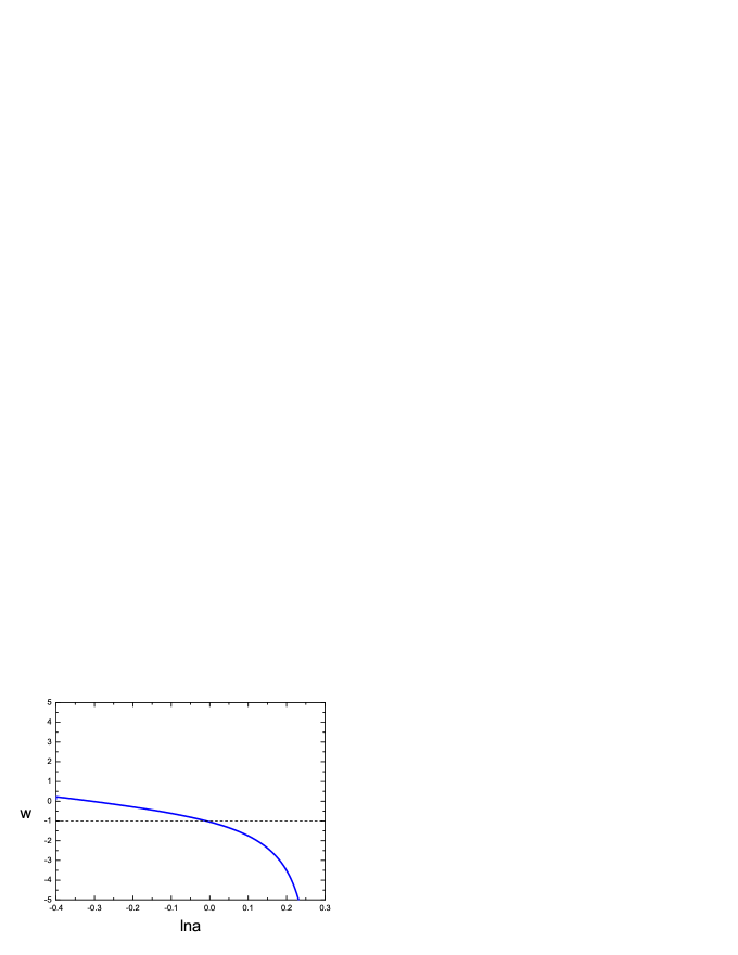
Figure 1: Plot of the evolution of the EOS as a function of $\ln a$. In the numerical calculation, we have taken $V(\phi)=V_{0}e^{-\lambda\phi^{2}}$ with $V_{0}=0.8$, $\lambda=1$, $\alpha=1$, and $\beta=-0.8$. For the initial conditions we choose $\phi_{i}=0.9$, $\dot{\phi}_{i}=0.6$, $(\Box\phi)_{i}=\frac{d}{dt}(\Box\phi)_{i}=0$.

In Figure 2 we take a different potential for numerical calculations. One can see that the EOS crosses over $-1$ during the evolution. When we take $\beta$ positive Figure 3 shows the EOS starts with $w<-1$, crosses over $-1$ into the region of $w>-1$, then transits again to $w<-1$.

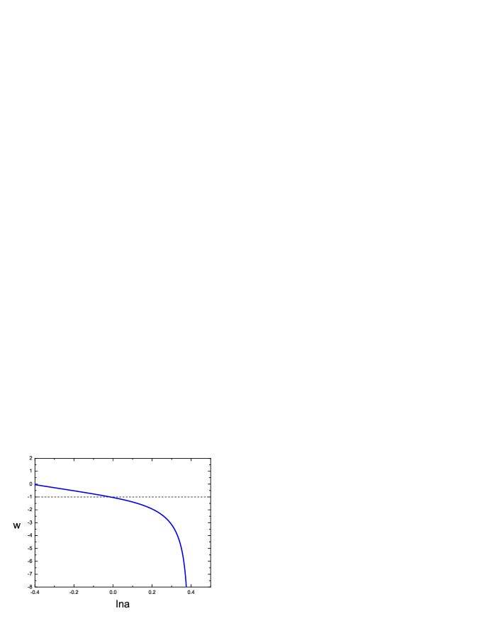
Figure 2: Plot of the evolution of the EOS as a function of $\ln a$. In the numerical calculation we take $V(\phi)=\frac{V_{0}}{e^{\lambda\phi}+e^{-\lambda\phi}}$, and $V_{0}=0.5$. For the model parameters we choose $\lambda=1$, $\alpha=1$, and $\beta=-0.8$. For the initial conditions we take $\phi_{i}=0.9$, $\dot{\phi}_{i}=0.6$, $(\Box\phi)_{i}=\frac{d}{dt}(\Box\phi)_{i}=0$.

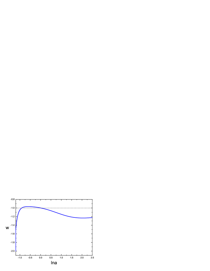
Figure 3: Plot of the evolution of the EOS as a function of $\ln a$. In the numerical calculation we take $V(\phi)=\frac{V_{0}}{e^{\lambda\phi}+e^{-\lambda\phi}}$, and $V_{0}=0.5$. For the model parameters we choose $\lambda=1$, $\alpha=1$, and $\beta=0.8$. For the initial conditions we take $\phi_{i}=0.9$, $\dot{\phi}_{i}=0.6$, $(\Box\phi)_{i}=\frac{d}{dt}(\Box\phi)_{i}=0$.

Now we study the stability property of this model by considering the quadratic perturbations. Consider a small perturbation $\pi$ around the background $\phi$,

$$\phi\rightarrow\phi(t)+\pi(t,{\bf x})~{},$$ (10)

where the background field $\phi$ in the FRW cosmology is spatially homogenous. Working with the action in (1) after a shift of the field in (10) and a tedious calculation we obtain the terms for the quadratic perturbations

$${}^{(2)}S \sim \int d^{4}x\sqrt{-g}~{}[(\frac{\alpha^{\prime}}{2}Vf^{-1}+\frac{\alpha^{\prime 2}}{2}Vf^{-3}\dot{\phi}^{2}+\frac{\beta^{\prime}}{2}Vf^{-1}+\frac{\beta^{\prime}}{2}\phi V_{\phi}f^{-1}-\frac{\beta^{\prime 2}}{4}\phi\Box\phi Vf^{-3})\dot{\pi}^{2}$$ (11)

$$-(\frac{\alpha^{\prime}}{2}Vf^{-1}+\frac{\beta^{\prime}}{2}Vf^{-1}+\frac{\beta^{\prime}}{2}\phi V_{\phi}f^{-1}-\frac{\beta^{\prime 2}}{4}\phi\Box\phi Vf^{-3})(\nabla\pi)^{2}$$

$$+...~{}].$$

Interestingly we notice that due to the positivity of the term $\frac{\alpha^{\prime 2}}{2}Vf^{-3}\dot{\phi}^{2}$ in this model if the coefficient of $(\nabla\pi)^{2}$ is positive, the term in front of $\dot{\pi}^{2}$ guarantee to be positively valued. The sound speed characterizing the stability property of the perturbations is given by

$$c_{s}^{2}=\frac{\frac{\alpha^{\prime}}{2}Vf^{-1}+\frac{\beta^{\prime}}{2}Vf^{-1}+\frac{\beta^{\prime}}{2}\phi V_{\phi}f^{-1}-\frac{\beta^{\prime 2}}{4}\phi\Box\phi Vf^{-3}}{\frac{\alpha^{\prime}}{2}Vf^{-1}+\frac{\alpha^{\prime 2}}{2}Vf^{-3}\dot{\phi}^{2}+\frac{\beta^{\prime}}{2}Vf^{-1}+\frac{\beta^{\prime}}{2}\phi V_{\phi}f^{-1}-\frac{\beta^{\prime 2}}{4}\phi\Box\phi Vf^{-3}}~{}.$$ (12)

If the $c_{s}^{2}$ lies in the range between $0$ and $1$ and the coefficient of $\dot{\pi}^{2}$ keeps positive, our model will be stable. In Figure 4 and Figure 5 we plot the $c_{s}^{2}$ and the coefficients of $\dot{\pi}^{2}$ respectively for the models above in the figures 1-3. From these figures one can see for these models $c_{s}^{2}$ are in the range of 0-1 and the coefficients of $\dot{\pi}^{2}$ are positive, so our models are stable.

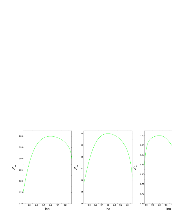
Figure 4: Plots of the sound speeds (from left to right) for the three models considered in this paper for the numerical calculations shown in Figure 1-3.

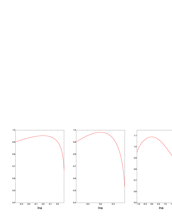
Figure 5: Plots of the coefficient of $\dot{\pi}^{2}$ (from left to right) for the three models considered in this paper for the numerical calculations shown in Figure 1-3.

III Conclusion and Discussion

The current cosmological observations indicate the possibility that the acceleration of the universe is driven by dark energy with EOS across $-1$, which if confirmed further in the future will challenge the theoretical model building of the dark energy. In this paper we have proposed a string-inspired model of dark energy through modifying the usual effective “Born-Infeld-type” description of tachyon dynamics. As shown in the present work, this modification by including a $\beta$ term in the action (1) is the key for the EOS crossing $-1$ during the evolution. Compared to other models with $w$ across $-1$ in the literature so far the present one is also economical in the sense that it involves a single scalar field such as a tachyon and has a motivation inspired from string theory consideration since the new features of this model for the dark energy could also be present in the realistic string theory if the whole tower of the higher derivative terms is fully included in the effective action.

- [1] S. Perlmutter et al., Astrophys. J. 483, 565 (1997); A. G. Riess et al., Astrophys. J. 116, 1009 (1998).
- [2] D. N. Spergel et al., Astrophys. J. Suppl. 148, 175 (2003).
- [3] A. G. Riess et al., Astrophys. J. 607, 665 (2004).
- [4] U. Seljak et al., Phys. Rev. D71, 103515 (2005).
- [5] D. N. Spergel et al., astro-ph/0603449.
- [6] A. G. Riess et al., astro-ph/0611572.
- [7] H. Li, M. Su, Z. Fan, Z. Dai, and X. Zhang, astro-ph/0612060.
- [8] G.-B. Zhao et al, astro-ph/0612728; H. Wei, N. Tang, and S. N. Zhang, astro-ph/0612746; J. Zhang, X. Zhang, and H. Liu, astro-ph/0612642; U. Alam, V. Sahni, and A. A. Starobinsky, astro-ph/0612381; Y.-G. Gong, and A. Wang, astro-ph/0612196; V. Barger, Y. Gao, D. Marfatia, astro-ph/0611775.
- [9] B. Feng, X. Wang and X. Zhang, Phys. Lett. B607, 35 (2005).
- [10] G.-B. Zhao, J.-Q. Xia, M. Li, B. Feng, and X. Zhang, Phys. Rev. D72, 123515 (2005).
- [11] R. R. Caldwell, M. Doran, Phys. Rev. D72, 043527 (2005); A. Vikman, Phys. Rev. D71, 023515 (2005); W. Hu, Phys. Rev. D71, 047301 (2005).
- [12] M. Li, B. Feng, and X. Zhang, JCAP 0512, 002 (2005); X.-F. Zhang, and T.-T. Qiu, Phys. Lett. B642, 187 (2006).
- [13] H. Wei, and R.-G. Cai, Phys. Rev. D73, 083002 (2006).
- [14] R.-G. Cai, H.-S. Zhang, and A. Wang, Commun. Theor. Phys. 44, 948 (2005); P. S. Apostolopoulos, and N. Tetradis, Phys. Rev. D74, 064021 (2006); H.-S. Zhang, and Z.-H. Zhu, Phys. Rev. D75, 023510 (2007).
- [15] B. Feng, M. Li, Y. Piao, and X. Zhang, Phys. Lett. B634, 101 (2006); X.-F. Zhang, H. Li, Y.-S. Piao, and X. M. Zhang, Mod. Phys. Lett. A21, 231 (2006); Z. Guo, Y. Piao, X. Zhang, and Y.-Z. Zhang, Phys. Lett. B608, 177 (2005); H. Li, B. Feng, J.-Q. Xia, and X. Zhang, Phys. Rev. D73, 103503 (2006); I. Y. Aref’eva, A. S. Koshelev, and S. Yu. Vernov, Phys. Rev. D72, 064017 (2005); Z.-K. Guo, Y.-S. Piao, X. Zhang, and Y.-Z. Zhang, astro-ph/0608165; Y.-F. Cai, H. Li, Y.-S. Piao, and X.-M. Zhang, Phys. Lett. B646, 141 (2007), arXiv:gr-qc/0609039; W. Zhao, and Y. Zhang, Phys. Rev. D73, 123509 (2006); M. R. Setare, Phys. Lett. B641, 130 (2006); E. O. Kahya, and V. K. Onemli, gr-qc/0612026; X. Zhang, and F.-Q. Wu, Phys. Rev. D72, 043524 (2005).
- [16] A. A. Gerasimov and S. L. Shatashvili, JHEP 0010, 034 (2000).
- [17] D. Kutasov, M. Marino and G. W. Moore, JHEP 0010, 045 (2000).
- [18] D. Kutasov, M. Marino and G. W. Moore, arXiv:hep-th/0010108.
- [19] N. Barnaby, T. Biswas and J. M. Cline, arXiv:hep-th/0612230.
- [20] P. Mukhopadhyay and A. Sen, JHEP 0211, 047 (2002).
- [21] A. Sen, JHEP 0204, 048 (2002); A. Sen, JHEP 0207, 065 (2002); A. Sen, Mod. Phys. Lett. A17, 1797 (2002); A. Sen, Int. J. Mod. Phys. A18, 4869 (2003).
- [22] G. Gibbons, Phys. Lett. B537, 1 (2002); S. Mukohyama, Phys. Rev. D66, 024009 (2002); D. Choudhury, D. Ghoshal, D. P. Jatkar, and S. Panda, Phys. Lett. B544, 231 (2002); T. Padmanabhan, Phys. Rev. D66, 021301 (2002); J. Hao, and X. Li, Phys. Rev. D66, 087301 (2002); J. S. Bagla, H. K. Jassal, and T. Padmanabhan, Phys. Rev. D67, 063504 (2003); E. J. Copeland, M. R. Garousi, M. Sami, and S. Tsujikawa, Phys. Rev. D71, 043003 (2005); M. C. Bento, O. Bertolami, and A. A. Sen, Phys. Rev. D67, 063511 (2003); K.-F. Zhang, W. Fang, and H.-Q. Lu, Int. J. Theor. Phys. 45, 1296, 2006.