Two Polyakov Loop Correlators
from D5-branes at Finite Temperature

Abstract

We study two Polyakov loop correlators in large $N$ limit of ${\cal{N}}=4$ super Yang-Mills theory at finite temperature using the AdS-Schwarzschild black hole. In the case that one of the two loops is of the anti-symmetric representation, we use D5-branes to evaluate them. The phase structure of these correlators is also examined. A previous result, derived in hep-th/9803135 and hep-th/9803137, is realized as a limiting case.

1 Introduction and summary

According to the pioneering works in Refs. 1) and 2), in the large ’t Hooft coupling regime, two Wilson loop correlators or two Polyakov loop correlators have been computed with the Nambu-Goto action of a classical open string in the dual geometry.${}^{3)-5),~{}18)}$ Gross and Ooguri pointed out in Ref. 5) that there exists a phase transition in this kind of correlator, which is best understood within the classical supergravity picture. This is because the topology of the open string worldsheet is an annulus, and the supergravity approximation breaks down when the circle of the annulus is of stringy size, $\simeq l_{s}$. Beyond that point, the supergraviton exchange between two loops becomes a more suitable description in the bulk. In other words, this change of topology gives rise to a phase transition.

Recently, due to the great progress made in our understanding of the holographical correspondence between Wilson loops of higher representations and D-branes,^7)-15) to realize the correlator using a D-brane/F-string system is thus natural. For example, at zero temperature, by making use of D-branes, the anti-symmetric-anti-symmetric and fundamental-anti-symmetric Wilson loop correlators are studied in Refs. 16) and 17), respectively, following the early works.^18)-22)

In this paper, we study the finite temperature fundamental-anti-symmetric Polyakov loop correlators, where the loops wind around the temporal circle. By constructing the D5-brane solution in the dual AdS-Schwarzschild black hole, we are able to compute the large $N$ limit of the correlator, realized as the NG action of a macroscopic string stretching between the very D5-brane and the AdS boundary. Since this D5-brane wraps an $S^{4}$ of the internal $S^{5}$, we find that the angular dependence in $S^{5}$ plays a role in the Coulomb-like behavior of the correlator, for small separation between two loops.

We also find that the string worldsheet remains in the annulus phase even if a maximal separation is reached; that is, the Gross-Ooguri transition does not take place. In addition, the known result presented in Ref. 3) and 4) is obtained by examining the limiting behavior of our solution.

The outline of this paper is as follows. In $\S 2$, the AdS-Schwarzschild black hole is reviewed. In $\S 3$, we construct the D5-brane solution embedded in the dual black hole geometry. In $\S 4$, we evaluate two Polyakov loop correlators using D5-brane solutions. In $\S 5$, comments on the Gross-Ooguri transition and limiting cases are given.

2 AdS-Schwarzschild black hole

We first describe the geometry of the five-dimensional AdS-Schwarzschild black hole, which is used to study the large $N$ boundary field theory, i.e. ${\cal{N}}=0$ four-dimensional SU($N$) Yang-Mills on $S^{1}\times R^{3}$. At high temperature, it effectively becomes $\text{QCD}_{3}$, because of the thermal circle $S^{1}$ (see Refs. 5) and 6)). In order to obtain the dual geometry, one can apply a Wick rotation to the Type IIB classical solution of $N$ coincident non-extremal D3-branes. What is of interest is its near horizon geometry, which is just the AdS-Schwarzschild black hole times an $S^{5}$. The metric is

$$\begin{aligned} \frac{ds^{2}}{\alpha^{\prime}}&=\frac{r^{2}}{R^{2}}(f(r)dt^{2}+\sum^{3}_{i=1}dx_{i}^{2})+R^{2}f(r)^{-1}\frac{dr^{2}}{r^{2}}+R^{2}(d\theta^{2}+\sin^{2}\theta d\Omega_{4}^{2}),\\ f(r)&=1-\frac{r_{0}^{4}}{r^{4}},~{}~{}~{}~{}R^{2}=\sqrt{4\pi g_{s}N}=\sqrt{\lambda},~{}~{}~{}~{}r_{0}=\pi\sqrt{4\pi g_{s}NT_{H}^{2}}.\end{aligned}$$ (1)

Despite the presence of $S^{5}$, the black hole has the topology of $D_{2}\times R^{3}$. To keep the near horizon manifold smooth, without any conical singularity, the Euclidean time direction is periodically identified as $t\sim t+\frac{1}{T}$, where $T_{H}=T/\pi$ is the Hawking temperature. In Refs. 3) and 4), by use of the dual AdS black hole, the quark-anti-quark potential $V_{q\bar{q}}$ in large $N$ limit is derived via the correlator of two temporal Wilson (Polyakov) loops, defined as

$$\begin{aligned} \langle P(0)P(d)\rangle\simeq e^{-V_{q\bar{q}}(d,T)/T}=e^{-S_{min}},\\ P=\frac{1}{N}\operatorname*{{\rm Tr}}U,~{}~{}~{}~{}~{}~{}~{}U:=P~{}e^{i\int_{0}^{1/T}dtA_{0}},\end{aligned}$$ (2)

where $d=|\triangle\vec{x}|$ is the separation between two loops in $R^{3}$. As found in Refs. 3) and 4), at low temperature (i.e. for $d\ll 1/T$), there exists a minimal surface bounded by two Polyakov loops, which dominates the connected correlator. Contrastingly, at high temperature (i.e. for $d\gg 1/T$), the inter-potential vanishes, due to the thermal screening.

In this paper, we consider another type of connected correlation function,

$$F(\theta_{k},d,\Theta)=\frac{\langle P_{k}(0,\theta_{k}){P_{\square}}(d,\Theta)\rangle-\langle P_{k}(0,\theta_{k})\rangle\langle{P_{\square}}(d,\Theta)\rangle}{\langle P_{k}(0,\theta_{k})\rangle},$$ (3)

where the subscript $k$ $({\square})$ denotes the $k$-th anti-symmetric (fundamental) representation. The quantity (3) is realized in the dual geometry as a string minimal surface stretching between the AdS boundary and a D5-brane. This is because the vev $\langle P_{k}(0,\theta_{k})\rangle$ is now related to a D5-brane carrying $k$ F-string charge, which probes the black hole geometry (1) and is wrapped on an $S^{4}$ at $\theta=\theta_{k}$. In addition, the angular dependence $\Theta$ in (3) arises from the fact that generally two loops are separated in $S^{5}$, e.g. $P(d,\Theta)$ is located at a point $n^{I}=(\cos\Theta,\sin\Theta,0,0,0,0)$ in $S^{5}$, where $n^{I}$ denotes the six-dimensional unit vector.

In large $N$ limit, $\langle P_{\square}(d,\Theta)\rangle=e^{-S_{min}}$ has been derived by using a fundamental string, which extends over $(t,r)$ with constant $(x_{i},\Omega_{5})$ coordinates. From the Nambu-Goto action (in the static gauge $\tau=t$),

$$\begin{aligned} S_{min}=\frac{1}{2\pi\alpha^{\prime}}\int d\tau d\sigma\sqrt{det~{}G},\end{aligned}$$ (4)

where $G$ is the induced metric, it is found that

$$S_{min}=\frac{1}{{2\pi}T}(r_{\infty}-r_{0}).$$ (5)

The above string configuration is referred to as the $disk$ phase, which is compared with the $annulus$ phase below (see Fig. 1).

3 D5-brane embedding

We now construct the D5-brane solution which is expected to be dual to the Polyakov loop of the $k$-th anti-symmetric representation on the boundary.

By rescaling as $(t,x_{i})\rightarrow{R^{2}}(t,x_{i})$, the metric (1) can be rewritten as

$${ds^{2}}=L^{2}\big{(}r^{2}f(r)dt^{2}+\frac{dr^{2}}{r^{2}f(r)}+r^{2}dx_{i}^{2}+d\theta^{2}+\sin^{2}\theta d\Omega_{4}^{2}\big{)},~{}~{}~{}L^{2}=\alpha^{\prime}\sqrt{\lambda}.$$ (6)

Then, using the Euclidean DBI action and the RR four-form

$$\begin{aligned} S_{bulk}&=T_{5}\int d^{6}\xi~{}e^{-\phi}\sqrt{det(G+{\cal F})}-iT_{5}\int{\cal F}\wedge C_{4},\\ C_{4}&=L^{4}(\frac{3}{2}\theta_{k}-\sin 2\theta_{k}+\frac{1}{8}\sin 4\theta_{k})~{}\text{vol}S^{4},\end{aligned}$$ (7)

as well as the ansatz (in the static gauge) for the D5-brane

$$(t,r,x_{i},\theta)=\big{(}\xi^{0},r(\xi^{1}),0,\theta_{k}\big{)},~{}~{}~{}~{}$$ (8)

we arrive at

$$\begin{aligned} S_{bulk}&=\int d\xi^{0}d\xi^{1}{\cal L},\\ {\cal L}&=T_{5}\frac{8\pi^{2}}{3}L^{4}\Big{(}\sin^{4}\theta_{k}\sqrt{L^{4}r^{\prime 2}+{\cal F}^{2}}-i{\cal F}(\frac{3}{2}\theta_{k}-\sin 2\theta_{k}+\frac{1}{8}\sin 4\theta_{k})\Big{)},\end{aligned}$$ (9)

where the prime denotes differentiation w.r.t. $\xi^{1}$, and we have integrated out the unit $S^{4}$ volume $(=\frac{8\pi^{2}}{3})$. The e.o.m. of ${\cal F}={\cal F}_{01}$ is

$$\frac{\delta{\cal L}}{\delta{\cal F}}=-\frac{i}{2\pi\alpha^{\prime}}k=T_{5}\frac{8\pi^{2}}{3}L^{4}\Big{(}\sin^{4}\theta_{k}~{}{\cal F}(L^{4}r^{\prime 2}+{\cal F}^{2})^{{-1}/{2}}-i(\frac{3}{2}\theta_{k}-\sin 2\theta_{k}+\frac{1}{8}\sin 4\theta_{k})\Big{)}.$$ (10)

Choosing the gauge in which $r=\xi^{1}$, we note that ${\cal F}=2\pi\alpha^{\prime}dA=-iL^{2}\cos\theta_{k}$. The F-string charge $k$ satisfies

$$k=\frac{2N}{\pi}(\frac{1}{2}\theta_{k}-\frac{1}{4}\sin 2\theta_{k}),$$ (11)

where, for small $\theta_{k}$, we have

$$k\simeq\frac{2N}{3\pi}\theta_{k}^{3}.$$ (12)

In summary, this D5-brane carries $k$ F-string charge and wraps spatially an $S^{4}$ as well as the $r$ direction from $r_{0}$ to $r_{\infty}$.

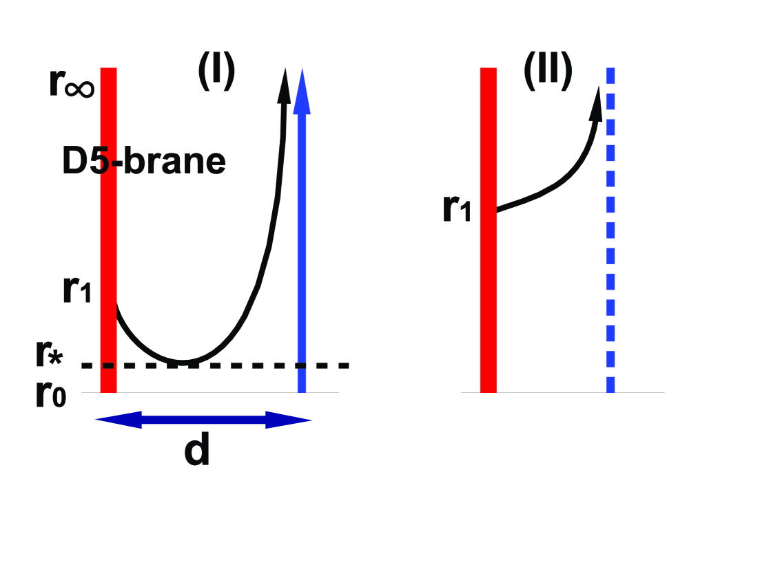
Figure 1: (I) A schematic picture of the annulus phase (the J-shaped string) with its tip at $r_{\ast}$ in the case $0\leq\theta_{k}\leq\frac{\pi}{2}$. Because the D5-brane is much heavier than the fundamental string, it is not pulled. $d$ denotes the separation between two Polyakov loops. The disk phase (blue arrow) is also depicted on the RHS. (II) The annulus phase depicted in the case $\frac{\pi}{2}<\theta_{k}\leq{\pi}$. Note that the slope at $r_{1}$ is determined by $\cos\theta_{k}$ as in (21).

4 Annulus phase

We now evaluate the annulus contribution. It is presented as a minimal surface bounded by the D5-brane constructed above and a fundamental Polyakov loop. Fig. 1 presents a schematic picture of this configuration. We use techniques similar to those utilized in Refs. 3), 4) and 17) to obtain the solution and its corresponding on-shell action.

4.1 Ansatz and equations of motion

Inserting the ansatz for the string worldsheet

$$\begin{aligned} t=\tau,\qquad r=r(\sigma),\qquad x_{1}\equiv x=x(\sigma),\qquad\theta=\theta(\sigma),\end{aligned}$$ (13)

we obtain the bulk Nambu-Goto action as

$$S_{bulk}=\frac{\sqrt{\lambda}}{2\pi T}\int_{\sigma_{1}}^{\sigma_{2}}d\sigma\sqrt{r^{\prime 2}+r^{4}f(r)x^{\prime 2}+r^{2}f(r)\theta^{\prime 2}},$$ (14)

where the prime denotes differentiation w.r.t. $\sigma$, and we have integrated out $\tau$.

At $\sigma=\sigma_{1}$, the worldsheet boundary is constrained to the rigid D5-brane and satisfies at least the following conditions:

$$x=0,\qquad\theta=\theta_{k}.$$ (15)

These are not all the conditions, however. Due to the D5-brane worldvolume gauge field excitation, we need to include another boundary term,

$$\begin{aligned} S_{bdy,1}=i\oint_{\sigma=\sigma_{1}}dt~{}A_{t}~{}+(\text{constant})=-i\frac{r(\sigma_{1})-r_{0}}{2\pi\alpha^{\prime}T}{\cal F},~{}&&A_{t}=-\frac{r}{2\pi\alpha^{\prime}}{\cal F}=\frac{irL^{2}\cos\theta_{k}}{2\pi\alpha^{\prime}}.\end{aligned}$$ (16)

The term “(constant)” ensures that $S_{bdy,1}=0$ when $r_{1}=r(\sigma_{1})$ reaches the horizon $r=r_{0}$, where the temporal circle of $t$ shrinks to a point, due to $g_{tt}(r_{0})=0$.

Now we derive boundary conditions obeyed by the worldsheet using a variational principle. The variation of the bulk action at $\sigma_{1}$ gives boundary terms as

$$\delta S_{bulk}|_{bdy,1}= -p_{r}\delta r-p_{x}\delta x-p_{\theta}\delta\theta,$$ (17)

where the momenta are

$$\begin{aligned} p_{r}=\frac{\sqrt{\lambda}}{2\pi T}\frac{r^{\prime}}{\sqrt{r^{\prime 2}+r^{4}f(r)x^{\prime 2}+r^{2}f(r)\theta^{\prime 2}}},\\ p_{x}=\frac{\sqrt{\lambda}}{2\pi T}\frac{r^{4}f(r)x^{\prime}}{\sqrt{r^{\prime 2}+r^{4}f(r)x^{\prime 2}+r^{2}f(r)\theta^{\prime 2}}},\\ p_{\theta}=\frac{\sqrt{\lambda}}{2\pi T}\frac{r^{2}f(r)\theta^{\prime}}{\sqrt{r^{\prime 2}+r^{4}f(r)x^{\prime 2}+r^{2}f(r)\theta^{\prime 2}}}.\end{aligned}$$ (18)

Further, the variation of $S_{bdy,1}$ is

$$\delta S_{bdy,1}=-\frac{L^{2}\cos\theta_{k}}{2\pi\alpha^{\prime}T}\delta r.$$ (19)

Thus, we obtain totally

$$\delta S_{bulk}|_{bdy,1}+\delta S_{bdy,1}=(-\frac{\sqrt{\lambda}\cos\theta_{k}}{2\pi T}-p_{r})\delta r-p_{x}\delta x-p_{\theta}\delta\theta=0.$$ (20)

The second and third terms vanish because of (15). The first term implies an additional boundary condition at $\sigma_{1}$, i.e.

$$-\cos\theta_{k}=\frac{r^{\prime}}{\sqrt{r^{\prime 2}+r^{4}f(r)x^{\prime 2}+r^{2}f(r)\theta^{\prime 2}}}.$$ (21)

Now we solve the equations of motion subject to the above boundary conditions. From (14), the equations of motion for $x$ and $\theta$ read

$$\begin{aligned} \frac{r^{4}f(r)}{\sqrt{r^{\prime 2}+r^{4}f(r)+r^{2}f(r)\theta^{\prime 2}}}=\alpha,\\ \frac{r^{2}f(r)\theta^{\prime}}{\sqrt{r^{\prime 2}+r^{4}f(r)+r^{2}f(r)\theta^{\prime 2}}}=\beta,\end{aligned}$$ (22)

where we have fixed the reparameterization of $\sigma$ as $x=\sigma$. Here, $\alpha$ and $\beta$ are integration constants. We can choose $\alpha\geq 0$ without loss of generality. Further, from (22), we have

$$\begin{aligned} \theta^{\prime}&=\gamma r^{2},~{}~{}~{}~{}~{}~{}~{}~{}~{}~{}\gamma=\frac{\beta}{\alpha},\\ r^{\prime}&=\pm\sqrt{\frac{r^{8}f(r)^{2}}{\alpha^{2}}-(1+\gamma^{2})r^{4}f(r)}.\end{aligned}$$ (23)

Therefore, the boundary condition (21) can be rewritten as

$$\frac{r_{1}^{\prime}}{\sqrt{r_{1}^{4}-r_{0}^{4}}}=\pm\sqrt{\frac{1+\gamma^{2}}{\tan\theta^{2}_{k}}}.$$ (24)

Note that the sign of $r^{\prime}_{1}$ depends on $\cos\theta_{k}$ in accordance with (21), and thus the $``+"$ branch in (24) corresponds to $\frac{\pi}{2}<\theta_{k}\leq\pi$, whereas the $``-"$ branch corresponds to $0\leq\theta_{k}\leq\frac{\pi}{2}$. On the basis of (23) and (24), we can explicitly express $r_{1}$ as

$$r^{4}_{1}-r^{4}_{0}=(\alpha^{2}+\beta^{2})\csc^{2}\theta_{k}.$$ (25)

This implies that when $\theta_{k}\ll 1$, $r_{1}$ is near $r_{\infty}$.

4.2 $0\leq\theta_{k}\leq\frac{\pi}{2}$ case

For $0\leq\theta_{k}\leq\frac{\pi}{2}$, (22) suggests that

$$\begin{aligned} \big{[}\frac{r^{\prime}}{r^{4}f(r)}\big{]}^{2}+\frac{1+\gamma^{2}}{r^{4}f(r)}=\frac{1+\gamma^{2}}{r_{\ast}^{4}f(r_{\ast})}=\text{constant}.\end{aligned}$$ (26)

In other words, $r_{\ast}$ is located where $\frac{dr}{d\sigma}=0$ (see Fig. 1) and is determined through (23) as $r^{4}_{\ast}=r_{0}^{4}+(\alpha^{2}+\beta^{2})$. Then, from (26), we obtain

$$\begin{aligned} dx&=\pm\frac{\sqrt{b^{4}-1}~{}dy}{r_{0}\sqrt{(y^{4}-1)(y^{4}-a^{4})}},\\ r_{0}\int^{d}_{0}dx&=\big{(}\int_{a}^{y_{1}}+\int_{a}^{\infty}\big{)}\frac{\sqrt{b^{4}-1}~{}dy}{\sqrt{(y^{4}-1)(y^{4}-a^{4})}},\end{aligned}$$ (27)

where we have chosen the proper branches in the second line and set

$$\begin{aligned} y=\frac{r}{r_{0}},~{}~{}~{}~{}~{}~{}a=\frac{r_{\ast}}{r_{0}},~{}~{}~{}~{}~{}~{}\frac{b^{4}-1}{a^{4}-1}=\frac{1}{1+\gamma^{2}}.\end{aligned}$$ (28)

As in Ref. 3), expressing (27) as an elliptical integral through a change of variable to $2w(y)=(y^{2}/a+a/y^{2})$, we arrive at

$$\begin{aligned} d=\frac{1}{4r_{0}~{}\sqrt{2}}\sqrt{\frac{b^{4}-1}{a^{3}}}\Big{[}(\int_{w(a)}^{\infty}+\int_{w(a)}^{w_{1}})\frac{dw}{\sqrt{(w-1)(w^{2}-w(a)^{2})}}\\ -(\int_{w(a)}^{\infty}+\int_{w(a)}^{w_{1}})\frac{dw}{\sqrt{(w+1)(w^{2}-w(a)^{2})}}\Big{]},\\ \rightarrow~{}~{}~{}d=\frac{1}{4r_{0}~{}\sqrt{w(a)}}\sqrt{\frac{b^{4}-1}{a^{3}}}\Big{[}K(\sqrt{\frac{w(a)+1}{2w(a)}})-K(\sqrt{\frac{w(a)-1}{2w(a)}})\\ +F(\chi_{-},\sqrt{\frac{w(a)+1}{2w(a)}})-F(\chi_{+},\sqrt{\frac{w(a)-1}{2w(a)}})\Big{]},\end{aligned}$$ (29)

where

$$\chi_{\pm}=\sin^{-1}\sqrt{\frac{w_{1}-w(a)}{w_{1}\pm 1}},~{}~{}~{}~{}w_{1}=w(y_{1}),~{}~{}~{}~{}y_{1}=\frac{r_{1}}{r_{0}}.$$ (30)

Note that $F$ is the elliptical integral of the first kind, while $K$ is its complete counterpart. From (23), we can also integrate out the $\theta$ part, obtaining

$$d\theta=\pm\gamma r_{0}\sqrt{b^{4}-1}\frac{y^{2}dy}{\sqrt{(y^{4}-1)(y^{4}-a^{4})}}.$$ (31)

Hence, we find

$$\begin{aligned} \Theta-\theta_{k}=\gamma r_{0}\sqrt{b^{4}-1}\frac{\sqrt{2a}}{8a}\Big{[}(\int_{w(a)}^{\infty}+\int_{w(a)}^{w_{1}})\frac{dw}{\sqrt{(w-1)(w^{2}-w(a)^{2})}}\\ +(\int_{w(a)}^{\infty}+\int_{w(a)}^{w_{1}})\frac{dw}{\sqrt{(w+1)(w^{2}-w(a)^{2})}}\Big{]},\\ =\gamma r_{0}\sqrt{\frac{b^{4}-1}{8(a^{2}+1)}}\Big{[}K(\sqrt{\frac{w(a)+1}{2w(a)}})+K(\sqrt{\frac{w(a)-1}{2w(a)}})\\ +F(\chi_{-},\sqrt{\frac{w(a)+1}{2w(a)}})+F(\chi_{+},\sqrt{\frac{w(a)-1}{2w(a)}})\Big{]},\end{aligned}$$ (32)

where the branches are chosen as in the case of (29). Note that (32) is invariant under $\Theta\to 2\theta_{k}-\Theta$, $\beta\to-\beta$. In summary, as seen from (29) and (32), $(d,\Theta)$ can be determined in terms of the three parameters $\theta_{k},\alpha$ and $\beta$, if they exist.

Finally, the total energy $E$ is proportional to the on-shell action, $S_{tot}=(S_{bulk}+S_{bdy,1})$:

$$E=\frac{\sqrt{\lambda}}{2\pi}r_{0}\Big{[}\big{(}\int_{a}^{\Lambda}+\int_{a}^{y_{1}}\big{)}dy\sqrt{\frac{y^{4}-1}{y^{4}-a^{4}}}-\cos\theta_{k}(y_{1}-1)-(\Lambda-1)\Big{]},~{}~{}~{}~{}~{}\Lambda=\frac{r_{\infty}}{r_{0}}.$$ (33)

Here, we have regularized $E$ by subtracting the term $(\Lambda-1)$. Note that $\frac{\sqrt{\lambda}}{2\pi}r_{0}(\Lambda-1)$ is precisely the disk phase energy mentioned in (5). The condition for the Gross-Ooguri transition to occur can be phrased as $E=0$, which means that the annulus phase has the same amount of energy as the disk phase.

4.3 $\frac{\pi}{2}<\theta_{k}\leq\pi$ case

For $\frac{\pi}{2}<\theta_{k}\leq\pi$, (25) suggests that $r^{\prime}$ in (23) never becomes zero, unlike in the previous case, in which there exists a tip at $r_{\ast}$. In the present case, $r$ increases monotonically from $r_{1}$ to infinity [see (II) of Fig. 1]. According to the above computations, $d$, $\Theta$ and $E$ here can be expressed as follows:

$$\begin{aligned} d=\frac{1}{4r_{0}~{}\sqrt{w(a)}}\sqrt{\frac{b^{4}-1}{a^{3}}}\Big{[}K(\sqrt{\frac{w(a)+1}{2w(a)}})-K(\sqrt{\frac{w(a)-1}{2w(a)}})\\ -F(\chi_{-},\sqrt{\frac{w(a)+1}{2w(a)}})+F(\chi_{+},\sqrt{\frac{w(a)-1}{2w(a)}})\Big{]},\\ \Theta-\theta_{k}=\gamma r_{0}\sqrt{\frac{b^{4}-1}{8(a^{2}+1)}}\Big{[}K(\sqrt{\frac{w(a)+1}{2w(a)}})+K(\sqrt{\frac{w(a)-1}{2w(a)}})\\ -F(\chi_{-},\sqrt{\frac{w(a)+1}{2w(a)}})-F(\chi_{+},\sqrt{\frac{w(a)-1}{2w(a)}})\Big{]},\\ E=\frac{\sqrt{\lambda}}{2\pi}r_{0}\Big{[}\int_{y_{1}}^{\Lambda}dy\sqrt{\frac{y^{4}-1}{y^{4}-y_{1}^{4}}}-\cos\theta_{k}(y_{1}-1)-(\Lambda-1)\Big{]}.\end{aligned}$$ (34)

5 Comments

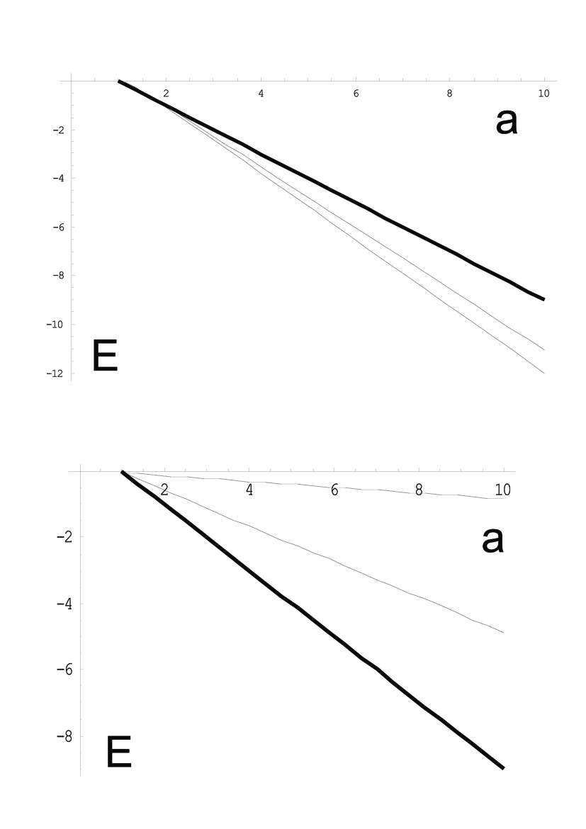
Figure 2: (Upper panel) The $E$-$a$ relation in the case $0\leq\theta_{k}\leq\pi/2$ obtained from (33). Here, $\theta_{k}=\pi/2,~{}\pi/3$, and $\pi/4$ are plotted from top to bottom. (Lower panel) The case $\pi/2<\theta_{k}\leq\pi$ obtained from (34). Here, $\theta_{k}=9\pi/10,~{}2\pi/3$, and $\pi/2$ are plotted from top to bottom. Note that the profiles of $\theta_{k}=\pi/2$ in the two cases coincide.

We now attempt to obtain an intuitive understanding of the above solutions by studying their asymptotic behavior. In (29) and (34), when $r_{1},a\to\infty$ (i.e. $\alpha\to\infty$ with $\beta$ fixed), due to the relation $K(\sqrt{\frac{1}{2}})\simeq 2.086$ (finite) and the condition $\chi_{\pm}\to 0$ (which allows us to ignore the elliptic integrals $F$), it is seen that $\Theta$ goes to $\theta_{k}$ for all given $\theta_{k}$, while the separation $d$ approaches zero in powers of $1/a$ as $\sim{1}/{a}+$ $\cal{O}$$({1}/{a^{5}})$.

In other words, at sufficiently low temperature (i.e. for $d\ll 1/T$), the leading string energy $E(d)$ is proportional to $\cos^{2}(\frac{\theta_{k}}{2})\sqrt{\lambda}/d$ with $0\leq\theta_{k}\leq{\pi}$, which differs from the fundamental-fundamental case treated in Refs. 3) and 4) by the factor $\cos^{2}(\frac{\theta_{k}}{2})$.

In addition to the case $a=\infty$ taken care of above, $d$ also approaches zero asymptotically like $\lim_{\epsilon\to 0}\big{(}\sqrt{\epsilon}\log\epsilon\big{)}\sim 0$ near the lower extreme, $a=1$. By noting that $d(a)$ is always positive for $1\leq a\leq\infty$, it is then straightforward to show that starting from zero separation (where $a=\infty$), we can reach an $a_{M}$ such that $d(a_{M})=d_{max}$ is the maximum.

Referring to Fig. 2, we see that for generic $\theta_{k}$, the phase transition occurs only at $a=1$, where $r_{1}=r_{\ast}=r_{0}$. This observation leads to the conclusion that by enlarging $d$ from zero, even when $d$ realizes its maximum at some $a=a_{M}>1$, the annulus phase still remains energetically favorable. This property differs from that in the fundamental-fundamental case, where the worldsheet splits at some $a_{M}\neq 1$.

It is also illuminating to check some limiting aspects of these solutions. We consider two situations: $\theta_{k}=0$ and $\frac{\pi}{2}$. As $k\rightarrow 1,$ it is seen that $\lim_{k\rightarrow 1}\theta_{k}\cong\left(\frac{3\pi}{2N}\right)^{1/3}\ll 1$ from (11). Then, from the relation $\theta_{k}\ll 1$, we find that $r_{1}\rightarrow\infty$ by virture of (25). Therefore, when $k=1$, we have

$$E =\frac{\sqrt{\lambda}}{2\pi T}r_{0}\Big{[}2\int_{a}^{\Lambda}dy\sqrt{\frac{y^{4}-1}{y^{4}-a^{4}}}-2(\Lambda-1)\Big{]},$$ (35)

$$d =\frac{1}{2r_{0}~{}\sqrt{w(a)}}\sqrt{\frac{b^{4}-1}{a^{3}}}\Big{[}K(\sqrt{\frac{w(a)+1}{2w(a)}})-K(\sqrt{\frac{w(a)-1}{2w(a)}})\Big{]},$$ (36)

$$\Theta =2\gamma r_{0}\sqrt{\frac{b^{4}-1}{8(a^{2}+1)}}\Big{[}K(\sqrt{\frac{w(a)+1}{2w(a)}})+K(\sqrt{\frac{w(a)-1}{2w(a)}})\Big{]}.$$ (37)

We thus see that the boundary term (16) provides exactly the subtraction term $(\Lambda-1)$, which can also be understood as a contribution from the denominator, $\lim_{k\to 1}\langle P_{k}(0,\theta_{k})\rangle$, of the correlator in (3). Note that (35) is simply the standard result derived in Refs. 3) and 4).

Next, in the case $\theta_{k}=\frac{\pi}{2}$, we see that $r_{1}=r_{\ast}$ from (25); i.e. the configuration is nothing but one-half of a full U-shaped string in the above $\theta_{k}=0$ case. In other words, its end on the D5-brane is now located at the tip where $\frac{dr}{d\sigma}=0$.

Acknowledgements

We are grateful to Satoshi Yamaguchi for many valuable comments on this manuscript.

References

- [1] S.-J. Rey and J.-T. Yee, “Macroscopic strings as heavy quarks in large N gauge theory and anti-de Sitter supergravity,” Eur. Phys. J. C22 (2001) 379–394, [arXiv:hep-th/9803001].
- [2] J. M. Maldacena, “Wilson loops in large N field theories,” Phys. Rev. Lett. 80 (1998) 4859–4862, [arXiv:hep-th/9803002].
- [3] S.-J. Rey, S. Theisen and J.-T. Yee, “ Wilson-Polyakov loop at finite temperature in large N gauge theory and anti-de Sitter supergravity,” Nucl. Phys. B527 (1998) 171–186, [arXiv:hep-th/9803135].
- [4] A. Brandhuber, N. Itzhaki, J. Sonnenschein and S. Yankielowicz, “Wilson loops in the large N limit at finite temperature,” Phys. Lett. B434 (1998) 36, [arXiv:hep-th/9803137].
- [5] D. J. Gross and H. Ooguri, “Aspects of large N gauge theory dynamics as seen by string theory,” Phys. Rev. D58 (1998) 106002, [arXiv:hep-th/9805129].
- [6] E. Witten, “Anti-de Sitter space, thermal phase transition, and confinement in gauge theories,” Adv. Theor. Math. Phys. 2 (1998) 505-532, [arXive:hep-th/9803131].
- [7] N. Drukker and B. Fiol, “All-genus calculation of Wilson loops using D-branes,” JHEP 02 (2005) 010, [arXiv:hep-th/0501109].
- [8] S. Yamaguchi, “Bubbling geometries for half BPS Wilson lines,” [arXiv:hep-th/0601089].
- [9] S. A. Hartnoll and S. Prem Kumar, “Multiply wound Polyakov loops at strong coupling,” Phys. Rev. D74 (2006) 026001, [arXiv:hep-th/0603190].
- [10] S. Yamaguchi, “Wilson loops of anti-symmetric representation and D5-branes,” JHEP 05 (2006) 037, [arXiv:hep-th/0603208].
- [11] J. Gomis and F. Passerini, “Holographic Wilson loops,” JHEP 08 (2006) 074, [arXiv:hep-th/0604007].
- [12] O. Lunin, “On gravitational description of Wilson lines,” JHEP 06 (2006) 026, [arXiv:hep-th/0604133].
- [13] J. Gomis and F. Passerini, “Wilson Loops as D3-Branes,” [arXiv:hep-th/0612022].
- [14] N. Drukker, S Giombi, R Ricci and D Trancanelli, “On the D3-brane description of some 1/4 BPS Wilson loops,” [arXive:hep-th/0612168].
- [15] J. Gomis and T. Okuda, “Wilson Loops, Geometric Transitions and Bubbling Calabi-Yau’s,” [arXiv:hep-th/0612190].
- [16] C. Ahn, “Two circular Wilson loops and marginal deformations,” [arXiv:hep-th/0606073].
- [17] T. -S. Tai and S. Yamaguchi, “Correlator of Fundamental and Anti-symmetric Wilson loops in AdS/CFT Correspondence,” [arXiv:hep-th/0610275].
- [18] K. Zarembo, “Wilson loop correlator in the AdS/CFT correspondence,” Phys. Lett. B459 (1999) 527–534, [arXiv:hep-th/9904149].
- [19] P. Olesen and K. Zarembo, “Phase transition in Wilson loop correlator from AdS/CFT correspondence,” [arXiv:hep-th/0009210].
- [20] H. Kim, D. K. Park, S. Tamarian and H. J. W. Muller-Kirsten, “Gross-Ooguri phase transition at zero and finite temperature: Two circular Wilson loop case,” JHEP 03 (2001) 003, [arXiv:hep-th/0101235].
- [21] G. Arutyunov, J. Plefka and M. Staudacher, “Limiting geometries of two circular Maldacena-Wilson loop operators,” JHEP 12 (2001) 014, [arXiv:hep-th/0111290].
- [22] N. Drukker and B. Fiol, “On the integrability of Wilson loops in : Some periodic ansatze,” JHEP 01 (2006) 056, [arXiv:hep-th/0506058].