Abstract

We study D- and DF-strings in a D3${\bar{\rm D}}3$ system by using Dirac-Born-Infeld type action. In the presence of an electric flux from the transverse direction, we discuss gravitating thick D-string solutions of a spatial manifold, ${\rm S}^{2}\times{\rm R}^{1}$, in which straight D-strings stretched along the R¹ direction are attached to the south and north poles of the two-sphere. There is a horizon along its equator, which means the structure of black strings is formed. We also discuss the BPS limit for thin parallel D- and DF-strings in both flat and curved spacetime. We obtain the BPS sum rule for an arbitrarily-separated multi-string configuration with a Gaussian type tachyon potential. At the site of each thin BPS D(F)-string, the pressure takes a finite value. We find that there exists a maximum deficit angle $\pi$ in the conical geometry induced by thin BPS D- and DF-strings.

1 Introduction

Cosmic strings have been extensively studied in the context of classical field theory, and Nielen-Olesen vortex-strings in the Abelian-Higgs model have been regarded as the representative example [1]. By solving the nonlinear field equations in the Abelian-Higgs model, one obtains point-like vortex solutions in 2-dimensional flat space. When such solitons gravitate in three dimensional spacetime, their 1-dimensional stringy objects could be interpreted as straight cosmic strings. The resulting conical geometry with deficit angle [2] has cosmological implications associated with possible lensing signatures, which are significantly different from those of standard gravitational lenses [3], or cosmological perturbations induced by the motion of cosmic strings.

A characteristic property of some topological solitons, including kinks, vortices, and monopoles, is saturation of the BPS bound [4]. In the case of the BPS vortices in the Abelian-Higgs model, an analysis of moduli space dynamics based on their $2n$ zero modes predicts 90 degree scattering in the head-on collision of two slowly-moving vortices [5]. This property has been confirmed by numerical analysis even for the fast-moving vortices [5], and it suggests an inter-commuting process of two colliding strings, which plays an important role in the evolution of a stringy network.

Another candidate for cosmic string is the superstring [6]. It shares almost all of the characteristic with vortex-strings in gauge theories with spontaneous symmetry breaking mechanism. As the topics of D-branes and the warped geometry have been developed, the idea of the cosmic superstring has recently been revived and, as an appropriate candidate, the D- and DF-strings have attracted much attention [7, 8, 9]. Concerning string cosmology [10], an intriguing setting is D- and DF-strings generated from the system of D3${\bar{\rm D}}3$, particularly those in the KKLMMT model [11].

For the generation of macroscopic D- and DF-strings from the system of D3${\bar{\rm D}}3$, a useful description can be made by employing the tachyon effective action [12, 13] as shown in the case of tachyon kinks [14]. When D3 and ${\bar{\rm D}}3$ are separated by a short distance, they start to approach each other due to mutual attraction and finally collide. Cosmologically, this period corresponds to an inflationary era in the early universe [15]. Instability of D${\bar{\rm D}}$ implies the presence of a complex tachyon field, and zero modes on D and ${\bar{\rm D}}$ correspond to two gauge fields of the U(1)$\times$U(1) symmetry. For description of this system, two kinds of effective actions have been proposed: One is that derived from boundary string field theory, which is very complicated [16, 17], and the other is that of a Dirac-Born-Infeld (DBI) type [12, 18]. As a U(1) symmetry is spontaneously broken, codimension-two D- or DF-branes are given as static vortex-string solutions in flat spacetime. These are nothing but straight D- or DF-strings (($p,q$)-strings) from the D3${\bar{\rm D}}3$ [19, 20]. In order to detect fossils of the cosmic superstrings, some remnants of macroscopic cosmic superstrings should survive in the present universe as far as their result is consistent with the data from the cosmic microwave background experiments. In this sense, D(F)-strings from D3${\bar{\rm D}}3$ is deemed more viable since they are produced after D-brane inflation [21].

Once cosmic superstrings are produced, various dynamical issues need to be understood, e.g., collisions between D-strings, F-strings, and DF-strings [22], formations of Y-junctions [8, 22, 23], probability of the reconnection of cosmic superstrings [24], and evolution of a cosmic DF-string network [25]. When the D${\bar{\rm D}}$ is dissociated, it decays into either perturbative closed string degrees [26] or nonperturbative open string degrees like cosmic D(F)-strings. In this sense, graviton production from D- or DF-strings is intriguing [27]. Concerning string cosmology based on flux compactification [28], D- and DF-strings in a warped geometry need also to be studied [29].

In section 2, we introduce the DBI type action of D3${\bar{\rm D}}3$ and investigate gravitating thick global D-strings with radial electric flux. On the spatial manifold ${\rm S}^{2}\times{\rm R}^{1}$, the straight strings, stretched along the ${\rm R}^{1}$, are attached to both the south and north poles of the ${\rm S}^{2}$. A horizon is formed along the equator of the ${\rm S}^{2}$. Thus, the solution found is a black string solution [30, 31]. In section 3, through a systematic study, we demonstrate the saturation of the BPS sum rule in the thin-limit D- and DF-strings in both flat and curved spacetime. We derive a condition for the tachyon potential saturating the BPS sum rule of multi-D(F)-strings and show that Gaussian type tachyon potential saturates this BPS sum rule, consistent with the descent relation for codimension-two BPS branes. The resulting deficit angle for thin BPS D- and DF-strings has the maximum value of $\pi$. We conclude in section 4 with a summary of the obtained results and brief discussions for further study.

2 Gravitating D-strings with Electric Flux

A D3${\bar{\rm D}}$3 system coupled to gravity in their coincidence limit can be described by the DBI type action with U(1)$\times$U(1) gauge symmetry [12, 18]

$$S = S_{{\rm EH}}+S_{{\rm M}}$$ (2.1)

$$= \int d^{4}x\left\{\frac{\sqrt{-g}}{2\kappa^{2}}(R-2\Lambda)-2{\cal T}_{3}V(\tau)\left[\,\sqrt{-\det(X^{+}_{\mu\nu})}+\sqrt{-\det(X^{-}_{\mu\nu})}\,\,\right]\right\}\,,$$ (2.2)

where

$$X^{\pm}_{\mu\nu}=g_{\mu\nu}+F_{\mu\nu}\pm C_{\mu\nu}+({\overline{D_{\mu}T}}D_{\nu}T+{\overline{D_{\nu}T}}D_{\mu}T)/2.$$ (2.3)

In the action (2.2), we have a complex tachyon field $T=\tau e^{i\chi}$, two U(1) gauge fields $A_{\mu}$ and $C_{\mu}$ with their field strength tensor $F_{\mu\nu}=\partial_{\mu}A_{\nu}-\partial_{\nu}A_{\mu}$ and $C_{\mu\nu}=\partial_{\mu}C_{\nu}-\partial_{\nu}C_{\mu}$, and the covariant derivative of the tachyon field $D_{\mu}T=(\partial_{\mu}-2iC_{\mu})T$.

Before beginning the detailed study, we briefly explain the terminology of the various strings of our interest. The D- and DF-strings stretched along the $z$-axis are distinguished by the nonvanishing fundamental (F) string charge density along the $z$-axis, $\Pi_{z}$. Since $\Pi_{z}$ is defined by the electric flux density conjugate to the $z$-component of gauge field $A_{z}$, $\Pi^{z}\equiv\frac{1}{2\sqrt{-g}}\frac{\delta S}{\delta\partial_{t}A_{z}}=\frac{1}{\sqrt{-g}}\frac{\delta S}{\delta E_{z}}$, the vortex-strings with the vanishing $E_{z}$ correspond to D-strings and those with the nonvanishing $E_{z}$ to DF-strings (or (p,q)-strings). Similarly to the vortex-strings in the Abelian-Higgs model, the global (local) D- and DF-string solutions are provided from the trivial (nontrivial) gauge field $C_{\mu}$ of vanishing (nonvanishing) field strength tensor $C_{\mu\nu}=0\,\,(C_{\mu\nu}\neq 0)$.

For the analysis of D- and DF-string solutions with the cylindrical symmetry, the monotonic connection of $V(\tau=0)=1$ and $V(\tau=\infty)=0$ is enough [32]. For numerical analysis, we use a specific form of the potential satisfying all of the above conditions

$$V(\tau)=\frac{1}{{\rm cosh}\left(\frac{\tau}{R}\right)}.$$ (2.4)

Since we are interested in straight black D-strings, it is convenient to use cylindrical coordinates $(t,r,\theta,z)$ in curved spacetime. To be specific we take into account the simplest form with translational symmetry along the $z$-direction:

$$ds^{2}=-N(r)^{2}dt^{2}+dz^{2}+b(r)(dr^{2}+r^{2}d\theta^{2}).$$ (2.5)

Under the metric (2.5), the complex tachyon field $T$ with $n$ vortices superimposed at the origin has

$$T=\tau(r)e^{in\theta}.$$ (2.6)

We assume the fundamental strings stretched along a transverse direction at $r=0$. In the next section, we consider additionally those superposed along the straight cosmic D-strings. Their string charge densities couple to the following components of electric fields, respectively:

$$F_{tr}(r)=E_{r}(r),\quad F_{tz}(r)=E_{z}(r).$$ (2.7)

To change global strings of our interest to local strings, we can turn on the angular component of the other U(1) gauge field $C_{\mu}$ and the corresponding field strength tensor $C_{\mu\nu}$ as

$$C_{\mu}=\delta_{\mu\theta}C_{\theta}(r),\qquad C_{r\theta}=C_{\theta}^{\prime}.$$ (2.8)

Substitution of the metric and ansätze, (2.5)–(2.8), leads to the equations of motion. The equation of motion for the tachyon amplitude $\tau$ is

$$\frac{d}{dr}\left\{\frac{\sqrt{-g}V}{\sqrt{X}}\left[1+\frac{\tau^{2}}{br^{2}}(n-2C_{\theta})^{2}\right]\frac{\tau^{\prime}}{b}\left(1-\frac{E_{z}^{2}}{N^{2}}\right)\right\}$$ (2.9)

$$-\frac{\sqrt{-g}V}{\sqrt{X}}\left[\left(1-\frac{E_{z}^{2}}{N^{2}}\right)\left(1+\frac{\tau^{{}^{\prime}2}}{b}\right)-\frac{E_{r}^{2}}{N^{2}b}\right]\frac{\tau(n-2C_{\theta})^{2}}{br^{2}}=\sqrt{-g}\sqrt{X}~{}\frac{dV}{d\tau},$$

and that for the gauge field $C_{\theta}$ is

$$\frac{d}{dr}\left[\frac{\sqrt{-g}V}{\sqrt{X}}\left(1-\frac{E_{z}^{2}}{N^{2}}\right)\frac{{C_{\theta}^{\prime}}^{2}}{b^{2}r^{2}}\right]+2\frac{\sqrt{-g}V}{\sqrt{X}}\left[\left(1-\frac{E_{z}^{2}}{N^{2}}\right)\left(1+\frac{\tau^{{}^{\prime}2}}{b}\right)-\frac{E_{r}^{2}}{N^{2}b}\right]\frac{\tau^{2}(n-2C_{\theta})}{br^{2}}=0,$$ (2.10)

where $-g=N^{2}b^{2}r^{2}$ and the determinant $X$ is

$$X = \frac{-\det(X^{\pm}_{\mu\nu})}{-g}$$ (2.11)

$$= \left[1+\frac{\tau^{2}}{br^{2}}(n-2C_{\theta})^{2}\right]\left[\left(1-\frac{E_{z}^{2}}{N^{2}}\right)\left(1+\frac{{\tau^{\prime}}^{2}}{b}\right)-\frac{E_{r}^{2}}{N^{2}b}\right]+\left(1-\frac{E_{z}^{2}}{N^{2}}\right)\frac{{C_{\theta}^{\prime}}^{2}}{b^{2}r^{2}}.$$

The Bianchi identity, $\partial_{\mu}F_{\nu\rho}+\partial_{\nu}F_{\rho\mu}+\partial_{\rho}F_{\mu\nu}=0$, dictates that $E_{z}$ in (2.7) should be constant, and the conjugate momentum $\Pi^{z}$ of $A_{z}$ is given by

$$\Pi^{z}\equiv\frac{1}{\sqrt{-g}}\frac{\delta S}{\delta E_{z}}=\frac{2{\cal T}_{3}V}{\sqrt{X}}\left\{\left[1+\frac{\tau^{2}}{br^{2}}(n-2C_{\theta})^{2}\right]\left(1+\frac{\tau^{{}^{\prime}2}}{b}\right)+\frac{C_{\theta}^{{}^{\prime}2}}{b^{2}r^{2}}\right\}\frac{E_{z}}{N^{2}}.$$ (2.12)

The equation for the gauge field $A_{\mu}$ reduces to $(Nbr\Pi^{r})^{\prime}=0$ which results in the expression of conjugate momentum $\Pi^{r}$ of $A_{r}$,

$$\Pi^{r}\equiv\frac{1}{\sqrt{-g}}\frac{\delta S}{\delta E_{r}}=\frac{Q}{Nbr},$$ (2.13)

where $Q$ is the fundamental string charge per unit length along the transverse direction. Therefore, $E_{r}(r)$ is given by an algebraic equation

$$\frac{E_{r}^{2}}{N^{2}b}=\frac{\left(1-\frac{E_{z}^{2}}{N^{2}}\right)\left\{\frac{C_{\theta}^{{}^{\prime}2}}{b^{2}r^{2}}+\left(1+\frac{\tau^{\prime 2}}{b}\right)\left[1+\frac{\tau^{2}}{br^{2}}\left(n-2C_{\theta}\right)^{2}\right]\right\}}{\left[1+\frac{\tau^{2}}{br^{2}}\left(n-2C_{\theta}\right)^{2}\right]\left\{1+b\left(\frac{2{\cal{T}}_{3}V}{Nb\Pi^{r}}\right)^{2}\left[1+\frac{\tau^{2}}{br^{2}}\left(n-2C_{\theta}\right)^{2}\right]\right\}}.$$ (2.14)

Since the fundamental strings of the charge $Q$ are not localized along the vortex-strings but stretched to the transverse direction, the D-string carrying the fundamental string charge $Q$ cannot be a DF-string but just be a D-string with electric flux. Among four nonvanishing $(t,r,\theta,z)$-components of the Einstein equations, we choose two independent equations for the metric functions, $N$ and $b$,

$$\frac{b^{{}^{\prime\prime}}}{b}+\frac{1}{r}\frac{b^{{}^{\prime}}}{b}-\left(\frac{b^{{}^{\prime}}}{b}\right)^{2}=-2b\left\{\Lambda+\frac{2\kappa^{2}{\cal T}_{3}V}{\sqrt{X}}\left[\left(1+\frac{\tau^{2}}{br^{2}}\left(n-2C_{\theta}\right)^{2}\right)\left(1+\frac{\tau^{{}^{\prime}2}}{b}\right)+\frac{C_{\theta}^{{}^{\prime}2}}{b^{2}r^{2}}\right]\right\},$$ (2.15)

$$\frac{N^{{}^{\prime\prime}}}{N}+\frac{1}{r}\frac{N^{{}^{\prime}}}{N}=-b\left\{2\Lambda+\frac{2\kappa^{2}{\cal T}_{3}V}{\sqrt{X}}\left[\left(1-\frac{E_{z}^{2}}{N^{2}}\right)\left(2+\frac{\tau^{{}^{\prime}2}}{b}+\frac{\tau^{2}}{br^{2}}\left(n-2C_{\theta}\right)^{2}\right)-\frac{E_{r}^{2}}{N^{2}b}\right]\right\}.$$ (2.16)

Since the analytic structure of the system is complicated as shown in (2.9)–(2.16), we begin with a simple but nontrivial case. Specifically, the global D-strings with electric flux are achieved by turning off the gauge field $C_{\theta}$ and the electric field $E_{z}$. A choice for the cosmological constant is $\Lambda=0$ since the minimum of the tachyon potential is naturally set to be $V(\tau=\infty)=0$. Then the equations of motion for our consideration are the tachyon equation (2.9) and the Einstein equations (2.15)–(2.16).

At the origin $(r=0)$, the boundary conditions are

$$\tau(0)=0\quad(n\neq 0),\qquad N(0)=N_{0},\qquad b(0)=b_{0},$$ (2.17)

where $N_{0}$ and $b_{0}$ can be set to be unity by a rescaling. Expansion of the fields near the origin gives

$$\frac{\tau(r)}{\tau_{0}} \approx r+\frac{Q^{2}}{12}\left[b_{0}\left(\kappa^{4}+(n^{2}-1)\frac{8{\cal T}_{3}^{2}}{Q^{4}}\right)+2\tau_{0}^{2}\left(\kappa^{4}+(n^{2}-1)\frac{4{\cal T}_{3}^{2}}{Q^{4}}\right)\right]r^{3}+\cdot\cdot\cdot,$$ (2.18)

$$\frac{N(r)}{N_{0}} \approx 1-\frac{|Q|\kappa^{2}b_{0}}{\sqrt{b_{0}+\tau_{0}^{2}}}\;r+\frac{1}{2}Q^{2}\kappa^{4}b_{0}\;r^{2}+\cdot\cdot\cdot,$$ (2.19)

$$\frac{b(r)}{b_{0}} \approx 1-2|Q|\kappa^{2}\sqrt{b_{0}+\tau_{0}^{2}}\;r+\frac{1}{2}Q^{2}\kappa^{4}\left(5b_{0}+4\tau_{0}^{2}\right)r^{2}+\cdot\cdot\cdot,$$ (2.20)

where $\tau_{0}$ is the only undetermined parameter. The tachyon field (2.18) is increasing from zero. The lapse function $N^{2}$ (2.19) and the conformal factor $b$ in front of the spatial part (2.20) are decreasing from constant values.

If we examine the tachyon equation (2.9) at a region of sufficiently large $r$, we easily conclude that the infinite tachyon amplitude at $r=\infty$ is impossible. It implies nonexistence of the D-string solution monotonically connecting the false symmetric vacuum, $\tau(0)=0$, and the true broken vacuum of the tachyon potential (2.4), $\tau(\infty)=\infty$, in curved spacetime. It is different from the case of flat spacetime. In this case, the tachyon amplitudes of D- and DF-strings reach an infinite value at the spatial infinity [19, 20]. Therefor e, a natural assumption is that its maximum value exists at a finite radial coordinate $r_{{\rm m}}$ such that $\tau(r_{{\rm m}})=\tau_{{\rm m}}$. A power series expansion supports this assumption as

$$\tau(r) \approx \tau_{{\rm m}}-\frac{b_{\rm m}\frac{4{\cal T}_{3}^{2}}{Q^{2}}e^{\frac{2\tau_{\rm m}}{R}}\left[\left(e^{\frac{2\tau_{\rm m}}{R}}-1\right)\left(b_{\rm m}r_{\rm m}^{2}+n^{2}\tau_{\rm m}^{2}\right)\right]-n^{2}R\tau_{\rm m}}{R\left(1+e^{\frac{2\tau_{\rm m}}{R}}\right)\alpha}(r-r_{\rm m})^{2}+\cdot\cdot\cdot,$$ (2.21)

$$\frac{N(r)}{N_{{\rm m}}} \approx \left(r-r_{\rm m}\right)-\frac{1}{2}\frac{N_{{\rm m}}^{2}}{r_{\rm m}}\left(r-r_{\rm m}\right)^{2}+\cdot\cdot\cdot,$$ (2.22)

$$\frac{b(r)}{b_{{\rm m}}} \approx 1+b_{{\rm m}1}\left(r-r_{\rm m}\right)+\left[\frac{b_{{\rm m}1}^{2}}{2}-\frac{b_{{\rm m}1}}{2r_{\rm m}}-\frac{|Q|\kappa^{2}\sqrt{b_{{\rm m}}\alpha}}{r_{\rm m}\left(1+e^{\frac{2\tau_{{\rm m}}}{R}}\right)}\right]\left(r-r_{\rm m}\right)^{2}+\cdots.$$ (2.23)

where

$$\alpha=1+e^{\frac{4\tau_{{\rm m}}}{R}}+e^{\frac{2\tau_{{\rm m}}}{R}}\left(2+\frac{16b_{{\rm m}}{\cal T}_{3}^{2}r_{\rm m}^{2}}{Q^{2}}+\frac{16{\cal T}_{3}^{2}}{Q^{2}}n^{2}\tau_{\rm m}^{2}\right).$$ (2.24)

The lapse function $N^{2}$ (2.22) hits zero at $r_{\rm m}$ and the time interval of a static observer to reach $r_{\rm m}$ is diverging, $\int dt\sim\int d\tau\ 1/N_{{\rm m}}(r-r_{\rm m})\stackrel{{\scriptstyle r\rightarrow r_{\rm m}}}{{\longrightarrow}}\infty$. This means that an event horizon is formed on the cylinder of radius $r_{\rm m}$ parallel to the $z$-axis and the obtained global ($C_{\theta}=0$) D-string ($E_{z}=0$) with electric flux ($E_{r}\neq 0$) is a black cosmic string [31]. Numerical analysis shows that it is indeed the case (See the solid line in Fig. 1).

Figure 1: Graphs of the lapse function $N(r)^{2}$ (solid line) and the conformal factor $b(r)$ (dashed line). Both of them are monotonically decreasing in the range of $0\leq r<r_{\rm m}$.

Since the conformal factor $b$ is decreasing near $r=r_{\rm m}$, the signature of $b_{{\rm m}1}$ in (2.23) is negative, which is supported by numerical analysis. Although it is decreasing to a nonzero value at $r_{{\rm m}}$, the radial distance from the origin, ${\cal R}(r)=\int_{0}^{r}dr^{{}^{\prime}}\,\sqrt{b(r^{{}^{\prime}})}\,$, is finite even at the horizon $r_{{\rm m}}$. Correspondingly the circumference along the angular coordinate $\theta$, $\ell(r)=r\sqrt{b(r)}$  , is also finite. Therefore, the geometry between $r=0$ and $r=r_{{\rm m}}$ is a hemisphere (See the left graph of Fig. 2), and, on this, the tachyon amplitude $\tau(r)$ grows from zero to the maximum value $\tau_{{\rm m}}$ as given in  (2.21) (See also the right graph of Fig. 2).

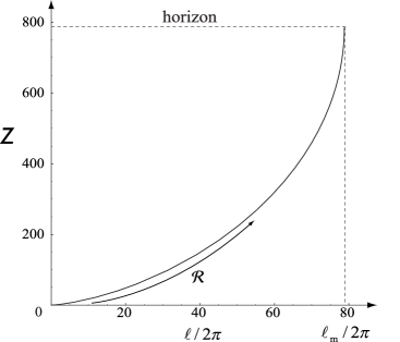
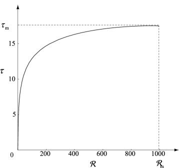
Figure 2: The left graph shows that the geometry embedded in three dimensions is a hemisphere and the right graph shows the tachyon amplitude $\tau(r)$. The vertical axis ${\sf Z}$ in the left graph is given by the relation, $d{\sf Z}^{2}=d{\cal R}^{2}-d(\ell/2\pi)^{2}$ with ${\sf Z}(r=0)=0$, $\ell(r_{\rm m})=\ell_{\rm m}$, and ${\cal R}(r_{\rm m})={\cal R}_{\rm m}$.

To understand local physical properties of the straight global D-strings with electric flux, we look into, in addition to the radial component of electric field $E_{r}$ (2.14), nonvanishing components of the energy-momentum tensor

$$-T^{t}_{\;t} = \frac{2{\cal T}_{3}V}{\sqrt{X}}\left[\left(1+\frac{\tau^{2}}{br^{2}}\left(n-2C_{\theta}\right)^{2}\right)\left(1+\frac{\tau^{{}^{\prime}2}}{b}\right)+\frac{C_{\theta}^{{}^{\prime}2}}{b^{2}r^{2}}\right],$$ (2.25)

$$-T^{z}_{\;z} = \frac{2{\cal T}_{3}V}{\sqrt{X}}\left[\left(1+\frac{\tau^{2}}{br^{2}}\left(n-2C_{\theta}\right)^{2}\right)\left(1+\frac{\tau^{{}^{\prime}2}}{b}-\frac{E_{r}^{2}}{N^{2}b}\right)+\frac{C_{\theta}^{{}^{\prime}2}}{b^{2}r^{2}}\right],$$ (2.26)

$$-T^{r}_{\;r} = \frac{2{\cal T}_{3}V}{\sqrt{X}}\left[1+\frac{\tau^{2}}{br^{2}}\left(n-2C_{\theta}\right)^{2}\right]\left(1-\frac{E_{z}^{2}}{N^{2}}\right),$$ (2.27)

$$-T^{\theta}_{\;\theta} = \frac{2{\cal T}_{3}V}{\sqrt{X}}\left[\left(1+\frac{\tau^{{}^{\prime}2}}{b}\right)\left(1-\frac{E_{z}^{2}}{N^{2}}\right)-\frac{E_{r}^{2}}{N^{2}b}\right],$$ (2.28)

and U(1) current $j^{\theta}$ for the gauge field $C_{\theta}$,

$$j^{\theta}=\frac{2{\cal T}_{3}V}{\sqrt{X}}\left[\left(1-\frac{E_{z}^{2}}{N^{2}}\right)\left(1+\frac{\tau^{{}^{\prime}2}}{b}\right)-\frac{E_{r}^{2}}{N^{2}b}\right]\frac{\tau^{2}(n-2C_{\theta})}{br^{2}}.$$ (2.29)

Insertion of the expansion of the fields near the origin (2.18)–(2.20) into (2.14) and (2.25)–(2.29) leads to

$$\frac{E_{r}}{N\sqrt{b}} \approx \sqrt{1+\frac{\tau_{0}^{2}}{b_{0}}}+\kappa^{2}|Q|\frac{\tau_{0}^{2}}{\sqrt{b_{0}}}\;r+{\cal O}(r^{2}),$$ (2.30)

$$T^{t}_{\;t} \approx -\frac{|Q|\sqrt{b_{0}+\tau_{0}^{2}}}{b_{0}}\;\frac{1}{r}-\frac{Q^{2}\kappa^{2}(b_{0}+2\tau_{0}^{2})}{b_{0}}$$ (2.31)

$$-\frac{|Q|^{3}\sqrt{b_{0}+\tau_{0}^{2}}}{16b_{0}}\left[\frac{32{\cal T}_{3}^{2}}{Q^{4}}(b_{0}+(2n^{2}-1)\tau_{0}^{2})+4\kappa^{4}\left(b_{0}+10\tau_{0}^{2}\right)\right]r+{\cal O}(r^{2}),$$

$$T^{z}_{\;z} \approx -\frac{4{\cal T}_{3}^{2}}{|Q|}\left(1+\frac{n^{2}\tau_{0}^{2}}{b_{0}}\right)\sqrt{b_{0}+\tau_{0}^{2}}\;r+{\cal O}(r^{2}),$$ (2.32)

$$T^{r}_{\;r} \approx -\frac{|Q|}{\sqrt{b_{0}+\tau_{0}^{2}}}\;\frac{1}{r}-\frac{\kappa^{2}Q^{2}b_{0}}{b_{0}+\tau_{0}^{2}}-\frac{|Q|^{3}}{16\left(b_{0}+\tau_{0}^{2}\right)^{3/2}}$$ (2.33)

$$\times\left[\frac{32{\cal T}_{3}^{2}}{Q^{4}}(b_{0}+\tau_{0}^{2})^{2}+4\kappa^{4}\left(b_{0}^{2}-5b_{0}\tau_{0}^{2}-2\tau_{0}^{4}\right)\right]r+{\cal O}(r^{2}),$$

$$T^{\theta}_{\;\theta} \approx -\frac{4{\cal T}_{3}^{2}}{|Q|}\sqrt{b_{0}+\tau_{0}^{2}}\;r+{\cal O}(r^{2}),$$ (2.34)

$$j^{\theta} \approx \frac{4n{\cal T}_{3}^{2}\tau_{0}^{2}\sqrt{b_{0}+\tau_{0}^{2}}}{|Q|b_{0}}\;r+{\cal O}(r^{2}).$$ (2.35)

Insertion of the power series expansion near the horizon at $r_{{\rm m}}$ (2.21)–(2.23) into (2.14) and (2.25)–(2.29) provides

$$\frac{E_{r}}{N\sqrt{b}} \approx \sqrt{\frac{1}{1+\frac{4{\cal T}_{3}^{2}}{Q^{2}}\beta{\rm sech}\frac{\tau_{\rm m}}{R}}}\left[1-\frac{\frac{r_{\rm m}}{b_{\rm m}}\left(2+b_{\rm m1}r_{\rm m}\right)}{\left(\frac{Q^{2}}{2{\cal T}_{3}^{2}}\cosh\frac{\tau_{\rm m}}{R}+2\beta\right)\cosh\frac{\tau_{\rm m}}{R}}\left(r-r_{\rm m}\right)+\cdots\right],$$ (2.36)

$$T^{t}_{\;t} \approx T^{r}_{\;r}$$ (2.37)

$$\approx -\frac{|Q|\rm sech\frac{\tau_{\rm m}}{R}}{\sqrt{2b_{\rm m}}\;r_{\rm m}}\sqrt{\gamma}\left[1-\frac{\left(2+b_{{\rm m}1}r_{\rm m}\right)\delta}{2r_{\rm m}\gamma}\left(r-r_{\rm m}\right)+\cdots\right],$$

$$T^{z}_{\;z} \approx -\frac{4\sqrt{2}{\cal T}_{3}^{2}\beta}{|Q|\sqrt{b_{\rm m}r_{\rm m}^{2}}\gamma}\Bigg{\{}1+\frac{(2b_{\rm m}+b_{{\rm m}1}r_{\rm m})}{(b_{\rm m}r_{\rm m}^{2}+n^{2}\tau_{\rm m}^{2})}$$ (2.38)

$$\times\frac{\left[b_{\rm m}r_{\rm m}^{2}\left(1-n^{2}\frac{8{\cal T}_{3}^{2}}{Q^{2}}+\cosh\frac{2\tau_{\rm m}}{R}\right)-n^{2}\tau_{\rm m}^{2}\delta\right]}{b_{\rm m}r_{\rm m}\gamma}\left(r-r_{\rm m}\right)+\cdots\Bigg{\}},$$

$$T^{\theta}_{\;\theta} \approx -\frac{4\sqrt{2}{\cal T}_{3}^{2}\sqrt{b_{\rm m}}r_{\rm m}{\rm sech}\frac{\tau_{\rm m}}{R}}{|Q|\sqrt{\gamma}}\left[1+\frac{(2+b_{{\rm m}1}r_{\rm m})\delta}{2r_{\rm m}\gamma}\left(r-r_{\rm m}\right)+\cdots\right],$$ (2.39)

$$j^{\theta} \approx \frac{4\sqrt{2}n{\cal T}_{3}^{2}\beta}{|Q|\sqrt{b_{\rm m}r_{\rm m}^{2}}\gamma}\left[1-\frac{(2+b_{{\rm m}1}r_{\rm m})\left(\frac{8{\cal T}_{3}^{2}}{Q^{2}}b_{\rm m}r_{\rm m}^{2}+\gamma\right)}{2r_{\rm m}\gamma}\left(r-r_{\rm m}\right)+\cdots\right].$$ (2.40)

where the parameters are

$$\beta = \left(b_{\rm m}r_{\rm m}^{2}+n^{2}\tau_{\rm m}^{2}\right){\rm sech}\frac{\tau_{\rm m}}{R},$$ (2.41)

$$\gamma = 1+\frac{8{\cal T}_{3}^{2}}{Q^{2}}(b_{\rm m}r_{\rm m}^{2}+n^{2}\tau_{\rm m}^{2})+\cosh\frac{2\tau_{\rm m}}{R},$$ (2.42)

$$\delta = 1+\frac{8{\cal T}_{3}^{2}}{Q^{2}}n^{2}\tau_{\rm m}^{2}\cosh\frac{2\tau_{\rm m}}{R}.$$ (2.43)

The radial component of electric field $\frac{E_{r}}{N\sqrt{b}}$ in (2.36) is rapidly decreasing from a constant at the origin (2.30) to the other constant value at the horizon $r_{\rm m}$ (See the left graph in Fig. 3). The fundamental string charge density $\Pi^{r}(r)$ in (2.13) starts from an infinite value at the origin, decreases to a finite value, and then diverges to infinity at the horizon $r_{\rm m}$ (See the right graph in Fig. 3). Therefore, the fundamental strings come from a transverse direction at the origin, flow along the latitude lines, and go out to the transverse direction on the equator of the hemisphere.

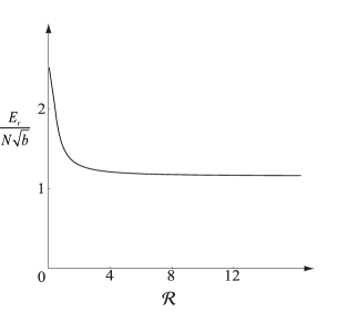
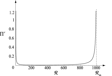
Figure 3: Graphs of the electric field $\frac{E_{r}}{N\sqrt{b}}$ (left) and the radial component of the conjugate momentum $\Pi^{r}$ (right) .

The energy density $-T^{t}_{\;t}$ and the radial component of pressure $T^{r}_{\;r}$ are divergent at the origin as given in (2.31) and (2.33) due to a contribution proportional to $|Q|$ from the fundamental strings. They also approach nonvanishing constants at the horizon as given in (2.37) (See Fig. 4).

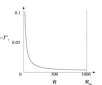
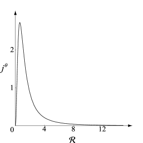
Figure 4: Graphs of the energy density $-T^{t}_{\;t}$(left) and $U(1)$ current $j^{\theta}$(right)

For the pressure along the string direction $T^{z}_{\;z}$, the angular components of pressure $T^{\theta}_{\;\theta}$, and the $U(1)$ current $j^{\theta}$, they start from zero at the origin as given in (2.32) and (2.34)–(2.35), vary monotonically, and then reach constant values at the horizon as given in (2.38)–(2.40). These nonvanishing constants at the horizon imply the existence of a short hair. This seems to be natural since the radial distance ${\cal R}$ from the location of the global D-strings to the horizon is finite.

Let us discuss possible physical configurations outside the horizon in what follows. At $r=\infty$, the following expressions can provide a consistent set of solutions:

$$\frac{\tau(r)}{\tau_{\infty}}\approx\frac{1}{r^{\frac{d}{2}-1}}\left[1+{\cal O}\left(1/r^{\frac{3d}{2}-1}\right)\right],$$ (2.44)

$$\frac{N(r)}{N_{\infty}}\approx 1-\frac{8b_{\infty}\kappa^{2}|Q|}{(d-2)^{2}\sqrt{4b_{\infty}+(d-2)^{2}\tau_{\infty}^{2}}}~{}\frac{1}{r^{\frac{d}{2}-1}}+{\cal O}\left(1/r^{\frac{3d}{2}-1}\right),$$ (2.45)

$$\frac{b(r)}{b_{\infty}}\approx\frac{1}{r^{d}}\left[1-\frac{4\kappa^{2}|Q|\sqrt{4b_{\infty}+(d-2)^{2}\tau_{\infty}^{2}}}{(d-2)^{2}}~{}\frac{1}{r^{\frac{d}{2}-1}}+{\cal O}\left(1/r^{\frac{3d}{2}-1}\right)\right].$$ (2.46)

A (in fact unique) natural boundary condition at $r=\infty$ is the vanishing tachyon amplitude and thus, (2.44) requires $d>2$. Subsequently, as $r\rightarrow\infty$, the circumference $\ell(r)$ along the angular coordinate $\theta$ goes to zero and the radial distance from the origin ${\cal R}(r)$ is finite. Since the asymptotic cylinder with finite $\ell(r=\infty)$ is excluded, a candidate of such a two-dimensional spatial compact manifold can uniquely be a two-sphere with $d=4$. Since this two-sphere is produced by the vortices at the origin (we call $r=0$ as the south pole), the topology of the two-sphere requires the vortices at infinity (we call $r=\infty$ as the north pole). In addition, a reflection symmetry between the south pole at $r=0$ and the north pole at $r=\infty$ should be assigned [33]. Through a coordinate redefinition near the north pole as $k/r\rightarrow r$, we fix the undetermined constants at infinity as $N_{\infty}=N_{0}$, $\tau_{\infty}=k\tau_{0}$, and $b_{\infty}=k^{2}b_{0}$. Therefore, the equator on the two-sphere should be located at the horizon $(r=r_{\rm m})$, where the lapse function $N^{2}$ vanishes. If the location of the horizon coincides with that of the equator [34], the circumference $\ell(r)$ reaches the maximum value along the equator, i.e., the condition $d\ell/dr|_{r=r_{{\rm m}}}=0$ fixes a coefficient as $b_{{\rm m}1}=-b_{{\rm m}}/r_{{\rm m}}$ in the conformal factor (2.23). Then, the number of undetermined parameters $(\tau_{{\rm m}},N_{{\rm m}},b_{{\rm m}})$ in (2.18)–(2.20), near the horizon, is three which is the same as that near the origin $(\tau_{0},N_{0},b_{0})$ in (2.21)–(2.23).

Substituting the asymptotic functional behavior (2.44)–(2.46) into the local physical quantities in (2.14) and (2.25)–(2.29), we have

$$\frac{E_{r}}{N\sqrt{b}} \approx \frac{\epsilon}{2\sqrt{b_{\infty}}}+\frac{\kappa^{2}|Q|\tau_{\infty}^{2}}{\sqrt{b_{\infty}}}\;r^{1-d/2}+{\cal O}(1/r^{\frac{3d}{2}-1}),$$ (2.47)

$$T^{t}_{\;t} \approx -\frac{|Q|\epsilon}{4b_{\infty}}\;r^{-1+d/2}-\frac{Q^{2}\kappa^{2}}{(d-2)^{2}b_{\infty}}\,\epsilon^{2}+{\cal O}(1/r^{\frac{d}{2}-1}),$$ (2.48)

$$T^{z}_{\;z} \approx -\frac{2{\cal T}_{3}^{2}}{|Q|}\left(1+\frac{n^{2}\tau_{\infty}^{2}}{b_{\infty}}\right)\,\epsilon\,r^{1-d/2}+{\cal O}(1/r^{\frac{3d}{2}-1}),$$ (2.49)

$$T^{r}_{\;r} \approx -\frac{2|Q|}{\epsilon}r^{-1+d/2}-\frac{16\kappa^{2}Q^{2}b_{\infty}}{(d-2)^{2}\epsilon^{2}}+{\cal O}(1/r^{\frac{d}{2}-1}),$$ (2.50)

$$T^{\theta}_{\;\theta} \approx -\frac{2{\cal T}_{3}^{2}}{|Q|}\,\epsilon\,r^{1-d/2}+{\cal O}(1/r^{\frac{3d}{2}-1}),$$ (2.51)

$$j^{\theta} \approx \frac{2n{\cal T}_{3}^{2}}{|Q|}\frac{\tau_{\infty}^{2}}{b_{\infty}}\,\epsilon\,r^{1-d/2}+{\cal O}(1/r^{\frac{3d}{2}-1}),$$ (2.52)

where $\epsilon=\sqrt{4b_{\infty}+(d-2)^{2}\tau_{\infty}^{2}}\,$. According to flipping $k/r\rightarrow r$ with $\tau_{0}=\tau_{\infty}/k$, $N_{0}=N_{\infty}$, and $b_{0}=b_{\infty}/k^{2}$, the coefficients of the leading terms near the north pole (2.47)–(2.52) coincide exactly with those near the south pole in (2.30)–(2.35). Therefore, the physical quantities and two-sphere itself preserve a symmetry under the exchange of the southern and northern hemispheres.

The various aforementioned investigations suggest the following (See also Fig. 5). The spatial manifold of coordinates $(r,\theta,z)$ is ${\rm S}^{2}\times{\rm R}^{1}$. There is a horizon along the equator of the two-sphere. Global D-strings with vorticity $n$, stretched along the $z$-axis $({\rm R}^{1})$, live at both the south and north poles. Fundamental strings come from a transverse direction to the south and north poles, flow to the equator along the latitudes, and go out to the transverse direction on the equator. Since the obtained horizon has a cylinder geometry, ${\rm S}^{1}\times{\rm R}^{1}$, surrounding each straight global D-string at the south or north pole, the obtained D-string at one hemisphere is identified as a straight black string to a static observer at the other hemisphere. The resultant picture is summarized in Fig. 5.

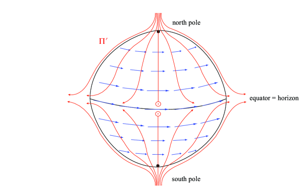
Figure 5: A schematic figure of global D-strings with fundamental strings on ${\rm S}^{2}\times{\rm R}^{1}$. The D-strings are on the south and north poles with the same vorticity. Fundamental strings from a transverse direction come in at the south and north poles and go out along the equator.

Since the spatial geometry is ${\rm S}^{2}\times{\rm R}^{1}$ and the field configuration keeps a translation symmetry along the string direction of ${\rm R}^{1}$, the dimensionally-reduced configuration is automatically constructed. To be specific, the system of our interest is D2${\bar{\rm D}}2$, and we obtain D-vortices (or D0-branes) with a radial electric field, which are located at both the north and south poles of ${\rm S}^{2}$. Since the horizon on the equator (${\rm S}^{1}$) divides two D-vortices, they are identified as two (1+2)-dimensional black holes.

3 BPS Limit of D- and DF-strings

In this section, we discuss the systematic derivation of the BPS limit for D- ($E_{z}=0$) and DF-strings ($E_{z}\neq 0$) stretched parallel to the $z$-direction. When we study the BPS limit of a solitonic object, rotational symmetry is not a necessary condition so that we do not assume it in the case of flat spacetime. We show that as expected, the BPS bound is saturated in the limit of zero thickness for global ($C_{\mu}=0$) D- and DF-strings without the radial component of electric field ($E_{r}=0$). In this section, we discuss first the case of flat spacetime and then that of the curved spacetime.

Once a BPS limit is saturated, a necessary condition is vanishing stress components, $T^{i}_{\;j}$. A softer condition would be the vanishing pressure ($P^{i}=T^{i}_{\;i}$) difference,

$$0=T^{i}_{\;i}-T^{|\epsilon_{ij}|j}_{\;|\epsilon_{ik}|k} = \frac{2{\cal T}_{3}V\sqrt{1-E_{z}^{2}}}{\sqrt{X|_{F=0}}}(\partial_{i}{\bar{T}}\partial_{i}T-\partial_{|\epsilon_{ij}|j}{\bar{T}}\partial_{|\epsilon_{ik}|k}T)$$ (3.2)

$$= \frac{{\cal T}_{3}V\sqrt{1-E_{z}^{2}}}{\sqrt{X|_{F=0}}}\left[(\overline{\partial_{i}T+i\epsilon_{ij}\partial_{j}T})(\partial_{i}T-i\epsilon_{ik}\partial_{k}T)\right.$$

$$\hskip 85.35826pt+\left.(\overline{\partial_{i}T-i\epsilon_{ij}\partial_{j}T})(\partial_{i}T+i\epsilon_{ik}\partial_{k}T)\right],$$

where $i,j=1,2$ (or $x,y$), $ii$ in $T^{i}_{\;i}$ denotes the $i$-th pressure component, and $X|_{F=0}=1+S_{ii}-\frac{1}{2}A_{ij}^{2}$ with $S(A)_{ij}\equiv\frac{1}{2}\left(\partial_{i}{\overline{T}}\partial_{j}T\pm\partial_{j}{\overline{T}}\partial_{i}T\right)$. The right-hand side of (3.2) should vanish. Then, we possibly identify the Cauchy-Riemann equation as the first-order Bogomolnyi equation for the BPS bound of arbitrary parallel D(F)-strings with upper signature (or anti-D(F)-strings with lower signature);

$$(\partial_{i}\pm i\epsilon_{ij}\partial_{j})T=0,\qquad(\,\partial_{i}\ln\tau=\pm\epsilon_{ij}\partial_{j}\chi\,).$$ (3.3)

We can easily confirm that substitution of the Bogomolnyi equation (3.3) leads to vanishing of the off-diagonal stress component $T^{i}_{\;j}\;(i\neq j)$ for both the strings and anti-strings;

$$T^{i}_{\;j} = \frac{{\cal T}_{3}V\sqrt{1-E_{z}^{2}}}{\sqrt{X|_{F=0}}}(\partial_{i}{\bar{T}}\partial_{j}T+\partial_{j}{\bar{T}}\partial_{i}T)$$ (3.5)

$$= \frac{{\cal T}_{3}V\sqrt{1-E_{z}^{2}}}{2\sqrt{X|_{F=0}}}\left[(\overline{\partial_{i}T\pm i\epsilon_{ik}\partial_{k}T})(\partial_{j}T\mp i\epsilon_{jl}\partial_{l}T)\right.$$

$$\hskip 82.51299pt\left.+(\overline{\partial_{j}T\pm i\epsilon_{jk}\partial_{k}T})(\partial_{i}T\mp i\epsilon_{il}\partial_{l}T)\right]$$

$$\stackrel{{\scriptstyle(\ref{Be1})}}{{=}} 0.$$ (3.6)

Here, in the second line (3.5), we used $\epsilon_{ik}\partial_{k}=\pm\partial_{j}$ and $\epsilon_{jk}\partial_{k}=\mp\partial_{i}$ for $i\neq j$.

For the $n$ straight strings spread arbitrarily on the $(x,y)$-plane, which are parallel along the $z$-direction, the phase of the tachyon field becomes

$$\chi=\pm\sum_{p=1}^{n}\tan^{-1}\frac{y-y_{p}}{x-x_{p}}.$$ (3.7)

Then, the tachyon amplitude $\tau$ is obtained as an exact solution of the Bogomolnyi equation (3.3),

$$\tau=\prod_{p=1}^{n}\tau_{{\rm BPS}}|{\bf x}-{\bf x}_{p}|,$$ (3.8)

where $\tau_{{\rm BPS}}$ is an integration constant and ${\bf x}-{\bf x}_{p}=(x-x_{p},y-y_{p})$. Due to the Bogomolnyi equation (3.8), we have

$$S_{xx} = S_{yy}=\mp iA_{xy}$$ (3.9)

$$= \tau_{{\rm BPS}}^{2}\prod_{p=1}^{n}(\tau_{{\rm BPS}}|{\bf x}-{\bf x}_{p}|)^{2}\sum_{q,r=1}^{n}\frac{\cos\theta_{qr}}{(\tau_{{\rm BPS}}|{\bf x}-{\bf x}_{q}|)\;(\tau_{{\rm BPS}}|{\bf x}-{\bf x}_{r}|)},$$

where $\theta_{qr}$ is the angle between the two vectors, $({\bf x}-{\bf x}_{q})$ and $({\bf x}-{\bf x}_{r})$. Plugging (3.7)–(3.9) into the pressure components provides $-T^{x}_{\;x}=-T^{y}_{\;y}=2{\cal T}_{3}V\sqrt{1-E_{z}^{2}}\,$. Only in the limit of zero thickness with $\tau_{{\rm BPS}}\rightarrow\infty$, the pressure components vanish everywhere except the string positions ${\bf x}_{p}=(x_{p},y_{p})$, i.e., $S_{xx}|_{{\bf x}={\bf x}_{q}}=0$ at ${\bf x}_{p}={\bf x}_{q}\;(p\neq q)$ and $-T^{x}_{\;x}|_{{\bf x}={\bf x}_{p}}=-T^{y}_{\;y}|_{{\bf x}={\bf x}_{p}}=2{\cal T}_{3}\sqrt{1-E_{z}^{2}}\,$. Since (3.3) gives $X=X|_{F=0}\left(1-E_{z}^{2}\right)=(1-E_{z}^{2})(1+S_{xx})^{2}$ and $\partial_{i}T-A_{ij}\partial_{j}T=\partial_{i}T(1+S_{xx})$, the left-hand side of the tachyon equation, $\partial_{i}\left[\frac{V}{2\sqrt{X}}(1-E_{z}^{2})(\partial_{i}T-A_{ij}\partial_{j}T)\right]=\sqrt{X}\partial V/\partial\bar{T}$, becomes $\sqrt{1-E_{z}^{2}}\;S_{xx}\partial V/\partial\bar{T}$. Moreover, $\partial V/\partial\bar{T}$ vanishes everywhere in the limit of $\tau_{{\rm BPS}}\rightarrow\infty$. Thus the first-order Bogomolnyi equation (3.3) is consistent with the second-order tachyon equation (2.9) for static BPS D- and DF-strings, equivalent to conservation of energy-momentum, $\partial_{j}T^{ji}=0$, for nontrivial solutions. Therefore, the tachyon configurations given by the solutions (3.7)–(3.8) of the Bogomolnyi equation (3.3) can be a BPS configuration only in the limit of infinite $\tau_{{\rm BPS}}$.

To see the BPS relation, let us look into the Hamiltonian density:

$${\cal H}=\sqrt{\Pi_{z}^{2}+4\Pi_{\bar{T}}\Pi_{T}+\left(\Pi_{\bar{T}}\partial_{i}{\bar{T}}+\Pi_{T}\partial_{i}T\right)^{2}+4{\cal T}_{3}^{2}V^{2}X|_{F=0}}\,\,,$$ (3.10)

where the corresponding conjugate momenta are

$$\Pi_{\bar{T}} = \frac{{\cal T}_{3}V}{\sqrt{X}}\left(\partial_{0}T-A_{0i}\partial_{i}T\right),$$ (3.11)

$$\Pi_{T} = \frac{{\cal T}_{3}V}{\sqrt{X}}\left(\partial_{0}\bar{T}+A_{0i}\partial_{i}\bar{T}\right),$$ (3.12)

$$\Pi_{z} = \frac{2{\cal T}_{3}V}{\sqrt{X}}E_{z}\left(X|_{F=0}\right).$$ (3.13)

For the static tachyon configurations, $\Pi_{{\bar{T}}}=\Pi_{T}=0$ from (3.11)–(3.12). Then, the Hamiltonian density (3.10) reproduces the BPS relation for thin DF-strings (($p,q$)-strings):

$${\cal H}=\sqrt{\Pi_{z}^{2}+\left(2{\cal T}_{3}V\sqrt{X|_{F=0}}\right)^{2}}\,\,,$$ (3.14)

where the BPS formula for D-strings, ${\cal H}=|2{\cal T}_{3}V\sqrt{X|_{F=0}}\,|$, is trivially obtained in the absence of the fundamental string charge density $\Pi_{z}=0$. Noticing that the energy density (2.25) is proportional to the electric flux density $\Pi^{z}$ (2.12) as

$${\cal H}=-\frac{\Pi^{z}}{E_{z}},$$ (3.15)

we easily read for the DF-strings (($p,q$)-strings) that the charge distribution of the fundamental string part coincides exactly with that of the D-string part, which is confined at each string site in the $(x,y)$-plane;

$$\Pi^{z}=-\frac{E_{z}}{\sqrt{1-E_{z}^{2}}}\;2{\cal T}_{3}V\sqrt{X|_{F=0}}\,.$$ (3.16)

Inserting the BPS configuration (3.7)–(3.8) into the energy density (3.25), we arrive at

$$\int d^{2}x\;{\cal H}=\frac{2{\cal T}_{3}}{\sqrt{1-E_{z}^{2}}}\int d^{2}x\;\lim_{\tau_{{\rm BPS}}\rightarrow\infty}V\left(\tau\right)\left(1+S_{xx}\right).$$ (3.17)

In the limit of infinite $\tau_{{\rm BPS}}$ with a rescaling to a dimensionless variable $|{\tilde{\bf x}}-{\tilde{\bf x}}_{p}|=\tau_{{\rm BPS}}|{\bf x}-{\bf x}_{p}|$, $S_{xx}$ is proportional to $\tau_{{\rm BPS}}^{2}$ as given in (3.9) and is dominating in (3.17) in comparison to unity. To obtain the BPS sum rule and the corresponding descent relation for the codimension-two D(F)-brane, ${\cal T}_{1}=\pi^{2}R^{2}{\cal T}_{3}/\sqrt{1-E_{z}^{2}}\,$, the required condition for $n$ D(F)-strings is

$$2{\cal T}_{1}|n| = \frac{2{\cal T}_{3}}{\sqrt{1-E_{z}^{2}}}\int d^{2}x\;\lim_{\tau_{{\rm BPS}}\rightarrow\infty}V\left(\tau\right)S_{xx}$$ (3.18)

$$= 2\frac{\pi^{2}R^{2}{\cal T}_{3}}{\sqrt{1-E_{z}^{2}}}|n|.$$ (3.19)

Let us find a class of tachyon potentials saturating the BPS sum rule from here on. As $\tau_{{\rm BPS}}$ approaches infinity for the arbitrarily-distributed $n$ thin BPS D(F)-strings, $V(\tau)|_{{\bf x}={\bf x}_{p}}=1$ and then $V(\tau)S_{xx}\propto(\tau_{{\rm BPS}})^{2n}$ diverges at each site of the strings ${\bf x}={\bf x}_{p}$. On the other hand, away from the string sites which have ${\bf x}\neq{\bf x}_{p}$ for all $p$, $V(\tau)=0$ and then $V(\tau)S_{xx}$ vanishes. Therefore, the constraint to the shape of the tachyon potential $V$ is

$$\lim_{\tau_{{\rm BPS}}\rightarrow\infty}V(\tau=\prod_{p=1}^{n}\tau_{{\rm BPS}}|{\bf x}-{\bf x}_{p}|)S_{xx}=\sum_{p=1}^{n}\delta^{(2)}({\bf x}-{\bf x}_{p}).$$ (3.20)

Suppose that we consider first the 1/cosh type tachyon potential (2.4) as a candidate. If we perform the integration for a single D(F)-string with $S_{xx}=\tau_{{\rm BPS}}^{2}$ before taking $\tau_{{\rm BPS}}\rightarrow\infty$, the integration produces

$$\int d^{2}(\tau_{{\rm BPS}}x)\;\frac{1}{\cosh(\frac{\tau_{{\rm BPS}}|{\bf x}-{\bf x}_{1}|}{R})}=2\pi K^{2}R^{2},\qquad\mbox{($K$ is the Catalan's constant)},$$ (3.21)

which is different from the descent relation (3.19). This result implies difficulty in employing this 1/cosh type tachyon potential as a BPS potential for BPS D(F)-strings, which is different from the case of tachyon kinks  [14]. Let us take into account the Gaussian type tachyon potential obtained in boundary string field theory [35]

$$V(\tau)=\exp\left(-\frac{\tau^{2}}{\pi R^{2}}\right).$$ (3.22)

Computation of the integration (3.18) after substituting the tachyon potential (3.22) reproduces correctly the descent relation (or the BPS sum rule) (3.19) for $n$ superimposed D(F)-strings with cylindrical symmetry, where we do not need to take to the limit of infinite $\tau_{{\rm BPS}}$. Let us consider the $n$ separated D(F)-strings where the distance between any pair of two strings is much larger than $1/\tau_{{\rm BPS}}$. In order to perform the integration (3.18), we look into a part of the integrand $S_{xx}$ (3.9) composed of a sum of the $n^{2}$ terms. For $n(n-1)$ terms with $q\neq r$, we show that the integration of such terms becomes zero in the limit of infinite $\tau_{{\rm BPS}}$. When ${\bf x}\neq{\bf x}_{s}~{}(s=1,2,...,n)$, the integrand of every term vanishes by taking the limit due to $\lim_{\tau_{{\rm BPS}\rightarrow\infty}}\exp(-{A}\tau_{{\rm BPS}}^{\;\;2n})B\tau_{{\rm BPS}}^{\;\;2n}\rightarrow 0$ for any nonvanishing finite $B$ and positive $A$. When ${\bf x}={\bf x}_{s}$, $\tau$ in (3.8) vanishes and $V(\tau)=1$ from (3.22). In addition, $S_{xx}\propto\left.|{\bf x}-{\bf x}_{s}|\right|_{{\bf x}={\bf x}_{s}}\rightarrow 0$ when $s$ is either $q$ or $r$ $(q\neq r)$, or $S_{xx}\propto\left.|{\bf x}-{\bf x}_{s}|^{2}\right|_{{\bf x}={\bf x}_{s}}\rightarrow 0$ when $s$ is neither $q$ nor $r$. Therefore, every $q\neq r$ term in (3.9) does not contribute to the integrated BPS sum rule (3.19) as far as every pair of two D(F)-strings is separated with a distance much larger than $1/\tau_{{\rm BPS}}$. If we finally take $\tau_{{\rm BPS}}\rightarrow\infty$, the integration values of all of the $q\neq r$ terms become zero irrespective of the nonvanishing values of their separation distances. For the $n$ terms with $q=r$ in $S_{xx}$ (3.9), the same argument as the case of $q\neq r$ is applied to the integrand in (3.18) at every ${\bf x}$ away from each string site, ${\bf x}\neq{\bf x}_{s}~{}(s=1,2,...,n)$. Now the source of the nonvanishing integration value for (3.18) comes from the $n$ terms of $q=r$ in $S_{xx}$ (3.18) and the contribution near each string site with $|{\bf x}-{\bf x}_{s}|\ll|{\bf x}_{q}-{\bf x}_{s}|,\;\;(q=r\neq s)$. Near ${\bf x}={\bf x}_{s}$, $\tau\rightarrow 0$ in (3.8), $V(\tau)\rightarrow 1$ from (3.22), and

$$S_{xx}\propto\left\{\begin{array}[]{ll}\left.\cdots|{\bf x}-{\bf x}_{s}|^{2}\cdots\right|_{{\bf x}={\bf x}_{s}}\rightarrow 0&\mbox{for~{}}q=r\neq s\\ \displaystyle{\lim_{\tau_{{\rm BPS}}\rightarrow\infty}\prod_{{p=1}\;(p\neq s)}^{n}(\tau_{{\rm BPS}}|{\bf x}_{q}-{\bf x}_{p}|)^{2}\rightarrow\infty}&\mbox{for~{}}q=r=s\end{array}\right..$$ (3.23)

We can perform this integration with sufficient accuracy since we first take the limit of infinite $\tau_{{\rm BPS}}$ for the BPS D(F)-strings. By using (3.23), in the limit of $\tau_{{\rm BPS}}\rightarrow\infty$, the integration in (3.18) is rewritten as

$$(\ref{sxc}) = \frac{2{\cal T}_{3}}{\sqrt{1-E_{z}^{2}}}\int d^{2}x\;\lim_{\tau_{{\rm BPS}}\rightarrow\infty}\sum_{s=1}^{n}\exp\left\{-\frac{1}{\pi R^{2}}\left[\prod_{p=1\;(p\neq s)}^{n}(\tau_{{\rm BPS}}|{\bf x}_{s}-{\bf x}_{p}|)^{2}\right](\tau_{{\rm BPS}}|{\bf x}-{\bf x}_{s}|)^{2}\right\}$$ (3.24)

$$\hskip 136.57323pt\times\tau_{{\rm BPS}}^{\;\;\;\;\;\;2}\left[\prod_{q=1\;(q\neq s)}^{n}(\tau_{{\rm BPS}}|{\bf x}_{s}-{\bf x}_{q}|)^{2}\right].$$

Since the integrand is a Gaussian type, this integration (3.24) is easily performed in a closed form and results in the BPS sum rule of our interest (3.19). Moreover, we consider the case that a part of the D(F)-strings are superimposed among the total $n$ D(F)-strings. Then, the above argument can be applied in the same manner since the Gaussian type potential reproduces correctly the BPS sum rule (3.19) for an arbitrary number of superimposed D(F)-strings as mentioned previously. In synthesis, the aforementioned analysis means that the Gaussian type tachyon potential (3.22) passes all of the requirements for the BPS sum rule (3.18)–(3.19) so that (3.22) is a BPS potential for parallel D(F)-strings.

For these D- and DF-strings, the boost symmetry along the string direction is sustained:

$$-T^{t}_{\;t}=-T^{z}_{\;z}=\frac{2{\cal T}_{3}V}{\sqrt{1-E_{z}^{2}}}\left(1+S_{xx}\right).$$ (3.25)

Though the above BPS limit was attained in the scheme of field theory, the BPS limit for thin D(F)-strings is consistent with the nature of a BPS D1-brane with zero thickness in string theory.

From now on, let us move to a discussion of the BPS bound in curved spacetime. With the metric (2.5) for curved spacetime, the pressure difference, $T^{r}_{\;r}-T^{\theta}_{\;\theta}$, becomes

$$0=T^{r}_{\;r}-T^{\theta}_{\;\theta}=\frac{2{\cal T}_{3}V}{\sqrt{\left(1+\frac{\tau^{{}^{\prime}2}}{b}\right)\left(1+n^{2}\frac{\tau^{2}}{r^{2}b}\right)}}\left(\tau^{{}^{\prime}}-n\frac{\tau}{r}\right)\left(\tau^{{}^{\prime}}+n\frac{\tau}{r}\right)$$ (3.26)

which leads to the same BPS equation in flat spacetime (3.3) with cylindrical symmetry and the linear ($|n|=1$) singular ($\tau_{{\rm BPS}}\rightarrow\infty$) tachyon profile (3.7)–(3.8). We check that the first-order equation and its would-be BPS configuration satisfies the second-order Euler-Lagrange equations. Since the time- and angular components of the energy-momentum conservation law is satisfied trivially $\nabla_{\mu}T^{\mu}_{\;t}=\nabla_{\mu}T^{\mu}_{\;\theta}=0$, the remaining radial component, $\nabla_{\mu}T^{\mu}_{\;r}=0$, becomes equivalent to the tachyon equation,

$$\frac{d}{dr}\left[\frac{2{\cal T}_{3}V}{\sqrt{X}}\left(1+\frac{\tau^{2}n^{2}}{br^{2}}\right)\right]+\frac{2{\cal T}_{3}V}{\sqrt{X}}\frac{N^{\prime}}{N}\left(1+\frac{\tau^{2}n^{2}}{br^{2}}\right)\frac{\tau^{{}^{\prime}2}}{b^{2}}-\left(\frac{1}{r}+\frac{b^{\prime}}{2b}\right)(T^{r}_{\;r}-T^{\theta}_{\;\theta})=0,$$ (3.27)

where $X=(1+\frac{\tau^{2}n^{2}}{br^{2}})(1+\frac{\tau^{{}^{\prime}2}}{b})$. Note that the Bogomolnyi equation $\tau^{\prime}=\tau n/r$ from (3.26) makes the equation (3.27) much simpler with $(1+\frac{\tau^{2}n^{2}}{br^{2}})/\sqrt{X}=1$. Its third term vanishes by (3.26) and the linear singular solution making $V=0$ for $r\neq 0$ still could be a consistent solution to (3.27) only if the boundary condition,

$$N^{\prime}|_{r=0}=0,$$ (3.28)

is satisfied. In fact, $N(r)$ and $b(r)$ should be determined by considering the Einstein equations (2.15)–(2.16). Substitution of (3.8) with $|n|=1$ and $\tau_{{\rm BPS}}=\infty$ results in

$$\frac{(rN^{\prime})^{\prime}}{rN}=b\kappa^{2}\left(T^{r}_{r}+T^{\theta}_{\theta}\right)=-2b\kappa^{2}{\cal T}_{3}V\left(\sqrt{\frac{1+\frac{\tau^{2}n^{2}}{br^{2}}}{1+\frac{\tau^{{}^{\prime}2}}{b}}}+\sqrt{\frac{1+\frac{\tau^{{}^{\prime}2}}{b}}{1+\frac{\tau^{2}n^{2}}{br^{2}}}}\,\right)=-4b\kappa^{2}{\cal T}_{3}V,$$ (3.29)

$$\frac{1}{2rb}\left(\frac{rb^{\prime}}{b}\right)^{\prime}=\kappa^{2}T^{t}_{t}=-2\kappa^{2}{\cal T}_{3}V\sqrt{\left(1+\frac{\tau^{2}n^{2}}{br^{2}}\right)\left(1+\frac{\tau^{{}^{\prime}2}}{b}\right)}=-\frac{\delta(r)}{br}\pi\kappa^{2}R^{2}{\cal T}_{3},$$ (3.30)

where the function $\delta(r)$ is defined as $\int_{0}^{\infty}dr\delta(r)=1$. For $r\neq 0$, the right-hand sides of (3.29)–(3.30) vanish due to the runaway property of the tachyon potential. Hence, the solutions for $r\neq 0$ are $N=N_{0}+N_{l}{\rm ln}r$ and $b=b_{0}r^{q}$, where $N_{0}$, $N_{l}$, $b_{0}$, and $q$ are integral constants. The nontrivial solution consistent with the required boundary condition in (3.28) is $N_{l}=0$. Then (3.29) requires a boundary condition

$$br|_{r=0}=0,$$ (3.31)

since $V(r=0)$ is unity while $N^{\prime}$ is zero in the entire region. Hence, $q$ in $b=b_{0}r^{q}$ should be greater than $-1$.

In (3.30), a constraint form of the tachyon potential for the desired descent relation is assumed as discussed in (3.17), $\int_{0}^{2\pi}d\theta\int_{0}^{\infty}dr\sqrt{g_{2}}(-T^{t}_{\;t})=2\pi^{2}R^{2}{\cal T}_{3}$, where $\sqrt{g_{2}}=br$ in this case. The left-hand side of (3.30) is $\frac{1}{2\sqrt{g_{2}}}\partial_{r}(\sqrt{g_{2}}\partial^{r}{\rm ln}b)=\frac{q}{2}\nabla^{2}{\rm ln}r=\frac{q}{2br}\delta(r)$. Comparison with the right-hand side of (3.30) yields $q=-2\pi\kappa^{2}R^{2}{\cal T}_{3}$, which provides a familiar conic spatial structure of the deficit angle, $\Delta=2\pi(1-|1+q/2|)=-q\pi$. Since $q>-1$, the deficit angle has, amazingly, the maximum value, $\pi$. Therefore, for the D- and DF-strings, the same BPS limit is saturated in curved spacetime, where the left-hand side of (3.30) leads to a topological quantity from the geometry side, an Euler number, and the right-hand side to a topological charge of a soliton, vorticity.

In curved spacetime, comparing with the D-strings, the only difference for the DF-string is a constant, $\sqrt{1-E_{z}^{2}/N^{2}}\,$. Since BPS bound is attained for the constant lapse function $N^{2}=N_{0}^{2}$, the previous BPS bound of the D-strings in curved spacetime is automatically applied to the case of DF-strings.

When the electric flux $E_{r}$ along the radial direction is turned on, any BPS bound is not saturated for these thick D-strings with electric flux. In addition, $-T^{t}_{\;t}\neq-T^{z}_{\;z}$ and thus the boost symmetry along the string direction breaks down to a translation symmetry along the $z$-axis.

For the Abelian Higgs model, the gauge field is indispensable. It converts the global vortices of the logarithmically divergent energy into the local vortices of finite energy. In addition, these local vortices can saturate the BPS bound under a specific form of scalar potential [4]. In the case of D- and DF-strings, their energy cannot be tamed by the gauge field $C_{\mu}$ and the BPS limit is achieved in the limit of thin vortices without the gauge field $C_{\mu}=0$. If we add the U(1) gauge field $C_{\mu}$ to make the global strings be local ones and introduce the electric field $E_{r}$ transverse to the strings, from Eqs. (2.25)–(2.28) we could expect such additions to hinder saturation of the BPS limit.

4 Conclusion and Discussion

We studied gravitating global D- and DF-strings in a D3${\bar{\rm D}}3$ system in the context of DBI type action of a complex tachyon and a DBI electromagnetic field. Einstein gravity with a vanishing cosmological constant has been assumed and only static straight strings have been considered.

When the electric flux in the transverse direction is turned on, the gravitated straight D-strings stretched along $z$-direction form a black string. The resultant space is the product of a two-sphere and a straight line, ${\rm S}^{2}\times{\rm R}^{1}$. The D-strings with the same vorticity lie on both the north and south poles of the two-sphere. The black string horizon is located on the equator so that the geometry of the horizon is S${}^{1}\times$R¹. From a transverse direction, fundamental strings also come into both the north and south poles, flow along the latitudes, and go out through the equator to the transverse direction. Although we constructed a static black string solution, their stability [36] needs to be addressed for the obtained structure of the black strings (or branes) [30, 31, 37].

We demonstrated explicitly and systematically the BPS limit for thin D- and DF-strings in both flat and curved spacetime. Almost all of the BPS properties are shared with Nielsen-Olesen vortices in the Abelian-Higgs model and their cosmic analogues, but the pressure components on the $(x,y)$-plane have a nonvanishing value, $2{\cal T}_{1}$, only at each D(F)-string site. We showed that a Gaussian type tachyon potential satisfied the BPS sum rule consistent with the descent relation for codimension-two BPS D(F)-strings. Our language describing cosmic D- and DF-strings was DBI-type action [12, 18]. It would be more intriguing to describe the strings in the context of boundary conformal field theory [38] or boundary string field theory [17] as has been done for tachyon kinks [39]. In the scheme of the DBI-type field theory of D3${\bar{\rm D}}3$ of our consideration, higher-derivative terms have been neglected. Thus, their effect may be tested to check whether or not the obtained BPS property is a genuine property of BPS D1- or D1F1-branes in the string theory.

Once the BPS limit is systematically obtained, dynamics of moduli space for the thin BPS D- and DF-strings [23] should be tackled, which has been expected to be different from that of the BPS Nielsen-Olesen vortices [5]. Then, their cosmological implication is expected to lead to interesting astrophysical phenomena in the early universe filled with cosmic superstrings. In addition to the study of the static objects and moduli space dynamics, full time evolution of D- and DF-strings by solving numerically the classical equations of motion needs further study [40].

References

- [1] For a review, see A. Vilenkin and E. P. S. Shellard, Cosmic strings and other topological defects, (Cambridge University Press, 1984) or T. W. B. Kibble, “Cosmic strings reborn?,” arXiv:astro-ph/0410073.
- [2] A. Vilenkin, “Gravitational field of vacuum domain walls and strings,” Phys. Rev. D 23, 852 (1981).
- [3] M. Sazhin et al., “CSL-1: a chance projection effect or serendipitous discovery of a gravitational lens induced by a cosmic string?,” Mon. Not. Roy. Astron. Soc. 343, 353 (2003) [arXiv:astro-ph/0302547]; M. V. Sazhin et al., “Gravitational lensing by cosmic strings: what we learn from the CSL-1 case,” Mon. Not. Roy. Astron. Soc. 376, 1731 (2007) [arXiv:astro-ph/0611744].
- [4] For a review, see N. Manton and P. Sutcliffe, Topological solitons, (Cambridge University Press, 2004).
- [5] E. P. S. Shellard and P. J. Ruback, “Vortex scattering in two-dimensions,” Phys. Lett. B 209, 262 (1988); P. J. Ruback, “Vortex string motion in the Abelian Higgs model,” Nucl. Phys. B 296, 669 (1988); T. M. Samols, “Hermiticity of the metric on vortex moduli space,” Phys. Lett. B 244, 285 (1990); “Vortex scattering,” Commun. Math. Phys. 145, 149 (1992); E. Myers, C. Rebbi and R. Strilka, “A study of the interaction and scattering of vortices in the Abelian Higgs (or Ginzburg-Landau) model,” Phys. Rev. D 45, 1355 (1992).
- [6] E. Witten, “Cosmic superstrings,” Phys. Lett. B 153, 243 (1985).
- [7] G. Dvali and A. Vilenkin, “Formation and evolution of cosmic D-strings,” JCAP 0403, 010 (2004) [arXiv:hep-th/0312007].
- [8] E. J. Copeland, R. C. Myers and J. Polchinski, “Cosmic F- and D-strings,” JHEP 0406, 013 (2004) [arXiv:hep-th/0312067].
- [9] For a review, see J. Polchinski, “Introduction to cosmic F- and D-strings,” Cargese 2004, String theory: From gauge interactions to cosmology, 229-253, arXiv:hep-th/0412244.
- [10] For a review, see J. M. Cline, “String cosmology,” arXiv:hep-th/0612129 or R. Kallosh, “Towards string cosmology,” Prog. Theor. Phys. Suppl. 163, 323 (2006), or S. H. Henry Tye, “Brane inflation: String theory viewed from the cosmos,” arXiv:hep-th/0610221.
- [11] S. Kachru, R. Kallosh, A. Linde, J. M. Maldacena, L. McAllister and S. P. Trivedi, “Towards inflation in string theory,” JCAP 0310, 013 (2003) [arXiv:hep-th/0308055].
- [12] A. Sen, “Dirac-Born-Infeld action on the tachyon kink and vortex,” Phys. Rev. D 68, 066008 (2003) [arXiv:hep-th/0303057].
- [13] A. Sen, “Tachyon dynamics in open string theory,” Int. J. Mod. Phys. A 20, 5513 (2005) [arXiv:hep-th/0410103].
- [14] C. Kim, Y. Kim and C. O. Lee, “Tachyon kinks,” JHEP 0305, 020 (2003) [arXiv:hep-th/0304180]; P. Brax, J. Mourad and D. A. Steer, “Tachyon kinks on non BPS D-branes,” Phys. Lett. B 575, 115 (2003) [arXiv:hep-th/0304197]; C. Kim, Y. Kim, O. K. Kwon and C. O. Lee, “Tachyon kinks on unstable Dp-branes,” JHEP 0311, 034 (2003) [arXiv:hep-th/0305092].
- [15] G. R. Dvali and S. H. H. Tye, “Brane inflation,” Phys. Lett. B 450, 72 (1999) [arXiv:hep-ph/9812483]; G. R. Dvali, Q. Shafi and S. Solganik, “D-brane inflation,” arXiv:hep-th/0105203. C. P. Burgess, M. Majumdar, D. Nolte, F. Quevedo, G. Rajesh and R. J. Zhang, “The inflationary brane-antibrane universe,” JHEP 0107, 047 (2001) [arXiv:hep-th/0105204]; J. Garcia-Bellido, R. Rabadan and F. Zamora, “Inflationary scenarios from branes at angles,” JHEP 0201, 036 (2002) [arXiv:hep-th/0112147]; S. H. S. Alexander, “Inflation from D - anti-D brane annihilation,” Phys. Rev. D 65, 023507 (2002) [arXiv:hep-th/0105032]; E. Halyo, “Inflation from rotation,” arXiv:hep-ph/0105341. G. Shiu and S. H. H. Tye, “Some aspects of brane inflation,” Phys. Lett. B 516, 421 (2001) [arXiv:hep-th/0106274]; C. Herdeiro, S. Hirano and R. Kallosh, “String theory and hybrid inflation / acceleration,” JHEP 0112, 027 (2001) [arXiv:hep-th/0110271]; B. Kyae and Q. Shafi, “Branes and inflationary cosmology,” Phys. Lett. B 526, 379 (2002) [arXiv:hep-ph/0111101].
- [16] P. Kraus and F. Larsen, “Boundary string field theory of the DD-bar system,” Phys. Rev. D 63, 106004 (2001) [arXiv:hep-th/0012198]; T. Takayanagi, S. Terashima and T. Uesugi, “Brane-antibrane action from boundary string field theory,” JHEP 0103, 019 (2001) [arXiv:hep-th/0012210].
- [17] N. T. Jones and S. H. H. Tye, “An improved brane anti-brane action from boundary superstring field theory and multi-vortex solutions,” JHEP 0301, 012 (2003) [arXiv:hep-th/0211180].
- [18] M. R. Garousi, “D-brane anti-D-brane effective action and brane interaction in open string channel,” JHEP 0501, 029 (2005) [arXiv:hep-th/0411222].
- [19] Y. Kim, B. Kyae and J. Lee, “Global and local D-vortices,” JHEP 0510, 002 (2005) [arXiv:hep-th/0508027].
- [20] I. Cho, Y. Kim and B. Kyae, “DF-strings from D3 D3-bar as cosmic strings,” JHEP 0604, 012 (2006) [arXiv:hep-th/0510218].
- [21] S. Sarangi and S. H. H. Tye, “Cosmic string production towards the end of brane inflation,” Phys. Lett. B 536, 185 (2002) [arXiv:hep-th/0204074]; T. Matsuda, “String production after angled brane inflation,” Phys. Rev. D 70, 023502 (2004) [arXiv:hep-ph/0403092]; N. Barnaby, A. Berndsen, J. M. Cline and H. Stoica, “Overproduction of cosmic superstrings,” JHEP 0506, 075 (2005) [arXiv:hep-th/0412095]; H. Firouzjahi and S. H. Tye, “Brane inflation and cosmic string tension in superstring theory,” JCAP 0503, 009 (2005) [arXiv:hep-th/0501099].
- [22] M. G. Jackson, N. T. Jones and J. Polchinski, “Collisions of cosmic F- and D-strings,” JHEP 0510, 013 (2005) [arXiv:hep-th/0405229].
- [23] E. J. Copeland, T. W. B. Kibble and D. A. Steer, “Collisions of strings with Y junctions,” Phys. Rev. Lett. 97, 021602 (2006) [arXiv:hep-th/0601153]; “Constraints on string networks with junctions,” Phys. Rev. D 75, 065024 (2007) [arXiv:hep-th/0611243].
- [24] A. Hanany and K. Hashimoto, “Reconnection of colliding cosmic strings,” JHEP 0506, 021 (2005) [arXiv:hep-th/0501031]; K. Hashimoto and D. Tong, “Reconnection of non-abelian cosmic strings,” JCAP 0509, 004 (2005) [arXiv:hep-th/0506022].
- [25] S. H. Tye, I. Wasserman and M. Wyman, “Scaling of multi-tension cosmic superstring networks,” Phys. Rev. D 71, 103508 (2005) [Erratum-ibid. D 71, 129906 (2005)] [arXiv:astro-ph/0503506]; E. J. Copeland and P. M. Saffin, “On the evolution of cosmic-superstring networks,” JHEP 0511, 023 (2005) [arXiv:hep-th/0505110]; M. Hindmarsh and P. M. Saffin, “Scaling in a SU(2)/Z(3) model of cosmic superstring networks,” JHEP 0608, 066 (2006) [arXiv:hep-th/0605014].
- [26] N. Lambert, H. Liu and J. M. Maldacena, “Closed strings from decaying D-branes,” JHEP 0703, 014 (2007) [arXiv:hep-th/0303139].
- [27] J. L. Cornou, E. Pajer and R. Sturani, “Graviton production from D-string recombination and annihilation,” Nucl. Phys. B 756, 16 (2006) [arXiv:hep-th/0606275].
- [28] S. Kachru, R. Kallosh, A. Linde and S. P. Trivedi, “De Sitter vacua in string theory,” Phys. Rev. D 68, 046005 (2003) [arXiv:hep-th/0301240].
- [29] H. Firouzjahi, L. Leblond and S. H. Henry Tye, “The (p,q) string tension in a warped deformed conifold,” JHEP 0605, 047 (2006) [arXiv:hep-th/0603161]; S. Thomas and J. Ward, “Non-Abelian (p,q) strings in the warped deformed conifold,” JHEP 0612, 057 (2006) [arXiv:hep-th/0605099]. H. Firouzjahi, “Dielectric (p,q) strings in a throat,” JHEP 0612, 031 (2006) [arXiv:hep-th/0610130].
- [30] G. T. Horowitz and A. Strominger, “Black strings and p-branes,” Nucl. Phys. B 360, 197 (1991).
- [31] N. Kim, Y. Kim and K. Kimm, “Global vortex and black cosmic string,” Phys. Rev. D 56, 8029 (1997) [arXiv:gr-qc/9707056]; “Charged black cosmic string,” Class. Quant. Grav. 15, 1513 (1998) [arXiv:gr-qc/9707011]; Y. Kim and S. H. Moon, “Gravitating sigma model solitons,” Phys. Rev. D 58, 105013 (1998) [arXiv:gr-qc/9803003].
- [32] A. Sen, “Universality of the tachyon potential,” JHEP 9912, 027 (1999) [arXiv:hep-th/9911116].
- [33] J. R. I. Gott, “Gravitational lensing effects of vacuum strings: Exact solutions,” Astrophys. J. 288 (1985) 422; B. Linet, “On the supermassive U(1) gauge cosmic strings,” Class. Quant. Grav. 7, L75 (1990); C. Kim and Y. Kim, “Vortices in Bogomolny limit of Einstein Maxwell Higgs theory with or without external sources,” Phys. Rev. D 50, 1040 (1994) [arXiv:hep-th/9401113].
- [34] C. Kim, Y. Kim and O. K. Kwon, “Tubular D-branes in Salam-Sezgin model,” JHEP 0405, 020 (2004) [arXiv:hep-th/0404163].
- [35] A. A. Gerasimov and S. L. Shatashvili, “On exact tachyon potential in open string field theory,” JHEP 0010, 034 (2000) [arXiv:hep-th/0009103]; D. Kutasov, M. Marino and G. W. Moore, “Some exact results on tachyon condensation in string field theory,” JHEP 0010, 045 (2000) [arXiv:hep-th/0009148].
- [36] R. Gregory and R. Laflamme, “Black strings and p-branes are unstable,” Phys. Rev. Lett. 70, 2837 (1993) [arXiv:hep-th/9301052]; “The instability of charged black strings and p-branes,” Nucl. Phys. B 428, 399 (1994) [arXiv:hep-th/9404071]; G. Kang and J. Lee, “Classical stability of black D3-branes,” JHEP 0403, 039 (2004) [arXiv:hep-th/0401225].
- [37] C. H. Lee, “Black string solutions with arbitrary tension,” Phys. Rev. D 74, 104016 (2006) [arXiv:hep-th/0608167].
- [38] J. Majumder and A. Sen, “Vortex pair creation on brane-antibrane pair via marginal deformation,” JHEP 0006, 010 (2000) [arXiv:hep-th/0003124].
- [39] C. Kim, Y. Kim, O. K. Kwon and H. U. Yee, “Tachyon kinks in boundary string field theory,” JHEP 0603, 086 (2006) [arXiv:hep-th/0601206].
- [40] G. N. Felder, L. Kofman and A. Starobinsky, “Caustics in tachyon matter and other Born-Infeld scalars,” JHEP 0209, 026 (2002) [arXiv:hep-th/0208019]; J. M. Cline and H. Firouzjahi, “Real-time D-brane condensation,” Phys. Lett. B 564, 255 (2003) [arXiv:hep-th/0301101]; N. Barnaby, “Caustic formation in tachyon effective field theories,” JHEP 0407, 025 (2004) [arXiv:hep-th/0406120]; O. K. Kwon and C. O. Lee, “Late time behaviors of an inhomogeneous rolling tachyon,” Phys. Rev. D 73, 126001 (2006) [arXiv:hep-th/0601236]; I. Cho, O. K. Kwon and C. O. Lee, “Evolution of Tachyon Kink with Electric Field,” JHEP 0704, 059 (2007) [arXiv:hep-th/0611053].