UFSCARF-TH-12-17

Exact solution and finite size properties
of the $U_{q}[osp(2|2m)]$ vertex models
W. Galleas and M.J. Martins

Universidade Federal de São Carlos
Departamento de Física
C.P. 676, 13565-905  São Carlos-SP, Brasil

We have diagonalized the transfer matrix of the $U_{q}[osp(2|2m)]$ vertex model by means of the algebraic Bethe ansatz method for a variety of grading possibilities. This allowed us to investigate the thermodynamic limit as well as the finite size properties of the corresponding spin chain in the massless regime. The leading behaviour of the finite size corrections to the spectrum is conjectured for arbitrary $m$. For $m=1$ we find a critical line with central charge $c=-1$ whose exponents vary continuously with the $q$-deformation parameter. For $m\geq 2$ the finite size term related to the conformal anomaly depends on the anisotropy which indicates a multicritical behaviour typical of loop models.

PACS numbers: 05.50+q, 02.30.IK

Keywords: Algebraic Bethe Ansatz, Lattice Models, Finite Size

December 2006

1 Introduction

Two-dimensional vertex models of statistical mechanics are nowadays considered classical paradigms of the theory of exactly solvable models [1]. Their statistical weights can be directly related to the elements of a $R$-matrix satisfying the Yang-Baxter equation invariant relative to the fundamental representations of $U_{q}[\mathcal{G}]$ quantum symmetries [2].

The thermodynamic limit properties of most vertex models derived from ordinary Lie algebras, such as the free-energy and the nature of the excitations, have been well examined over the past decades in the literature, see for instance [3, 4, 5, 6] and references therein. It is believed, for instance, that the massless regimes of these vertex models are described by the critical properties of Wess-Zumino-Witten field theories on the group $\mathcal{G}$ [7]. We remark, however, that at least one counter example to such common belief appears to occur in the $U_{q}[sp(2m)]$ vertex models [8].

By way of contrast, similar physical properties of the $U_{q}[\mathcal{G}]$ vertex models when $\mathcal{G}$ is a superalgebra have not yet been examined in details. The majority of the results concerning the possible universality classes of critical behaviour governing the massless phases in these systems have been concentrated on the $sl(n|m)$ symmetry [9, 10, 11]. Similar information for other superalgebras such as $osp(r|2m)$ has so far been restricted to the rational limit $q\rightarrow 1$ [12, 13, 14]. It is not yet clear, however, if the determined classes of universality are robust against $q$-deformations such as the cases of ungraded algebras.

In this paper we hope to start to bridge this gap by investigating the leading finite size corrections governing the eigenspectrum of the $U_{q}[osp(2|2m)]$ vertex models. These finite size properties have a direct relationship with the critical operator content of massless phases [15]. In order to do that we have diagonalized the respective row-to-row transfer matrix by means of the algebraic Bethe ansatz approach. We have considered explicitly all grading choices that are compatible with the underlying $U(1)$ symmetries of the $R$-matrix. This step will complement our previous efforts concerning the Bethe ansatz solution of the $U_{q}[osp(n|2m)]$ vertex models [16]. We recall that the exact solution for $n=2$ was not presented before [16] due to technical problems with the special grading considered in that work. Here we are able to circumvent such technicalities.

This paper is organized as follows. We start next section by describing the statistical weights of the $U_{q}[osp(2|2m)]$ vertex models. In section 3 we discuss the diagonalization of the corresponding row-to-row transfer matrix, within the algebraic Bethe ansatz method, for a variety of grading possibilities. In section 4 we use such grading freedom to choose the appropriate one in order to deal with the thermodynamic limit in the simplest possible manner. In section $5$ we study the finite size properties of the $U_{q}[osp(2|2m)]$ vertex models by both analytical and numerical approaches. This provides us the basis to conjecture, in the massless regime, the behaviour of the leading finite size corrections to the spectrum for general $m$. For $m=1$ these results indicate that the central charge of the underlying conformal field theory is $c=-1$. For $m\geq 2$, however, we find that the finite size term associated to the conformal central charge depends on the anisotropy coupling $q$. In Appendices A and B we describe the technical details entering the Bethe ansatz solution of a particular grading.

2 The $U_{q}[osp(2|2m)]$ vertex model

The $R$-matrix of the $U_{q}[osp(2|2m)]$ vertex model is defined on the tensor product of $Z_{2}$ graded spaces having two species of bosons and $2m$ species of fermions. The Grassmann parity $p_{\alpha}$ is used to distinguish the bosonic $p_{\alpha}=0$ and the fermionic $p_{\alpha}=1$ degrees of freedom.

To establish the statistical interpretation of this system it is important to know the structure of the $R$-matrix $R_{12}(\lambda)$ in appropriate coordinates such as the Weyl basis. This task is in general rather involved for superalgebras but recently some progresses towards this direction have been made [17, 18]. The Boltzmann weights of such systems can be conveniently written in terms of the standard relation [19],

$$R_{12}(\lambda)=P_{12}\check{R}_{12}(\lambda),$$ (1)

where $P_{12}$ is the graded permutator given by $P=\displaystyle\sum_{\alpha,\beta=1}^{N}(-1)^{p_{\alpha}p_{\beta}}\hat{e}_{\alpha\beta}\otimes\hat{e}_{\beta\alpha}$ and $\hat{e}_{\alpha\beta}$ denotes $N\times N$ matrices having only one non-null element with value 1 at row $\alpha$ and column $\beta$. The operator $\check{R}_{12}(\lambda)$ satisfies the following form of the Yang-Baxter equation,

$${\check{R}}_{12}(\lambda-\mu){\check{R}}_{23}(\lambda){\check{R}}_{12}(\mu)={\check{R}}_{23}(\mu){\check{R}}_{12}(\lambda){\check{R}}_{23}(\lambda-\mu).$$ (2)

which is insensitive to grading.

It turns out that the corresponding $\check{R}$-matrix of the $U_{q}[osp(2|2m)]$ vertex model, in terms of the Weyl basis, can be written as,

$${\check{R}}^{(0)}(\lambda) = \sum_{\stackrel{{\scriptstyle\alpha=1}}{{\alpha\neq\alpha^{\prime}}}}^{N_{0}}a_{\alpha}^{(0)}(\lambda)\hat{e}_{\alpha\alpha}\otimes\hat{e}_{\alpha\alpha}+b^{(0)}(\lambda)\sum_{\stackrel{{\scriptstyle\alpha,\beta=1}}{{\alpha\neq\beta,\alpha\neq\beta^{\prime}}}}^{N_{0}}(-1)^{p_{\alpha}^{(0)}p_{\beta}^{(0)}}\hat{e}_{\beta\alpha}\otimes\hat{e}_{\alpha\beta}$$ (3)

$$+{\bar{c}}^{(0)}(\lambda)\sum_{\stackrel{{\scriptstyle\alpha,\beta=1}}{{\alpha<\beta,\alpha\neq\beta^{\prime}}}}^{N_{0}}\hat{e}_{\alpha\alpha}\otimes\hat{e}_{\beta\beta}+c^{(0)}(\lambda)\sum_{\stackrel{{\scriptstyle\alpha,\beta=1}}{{\alpha>\beta,\alpha\neq\beta^{\prime}}}}^{N_{0}}\hat{e}_{\alpha\alpha}\otimes\hat{e}_{\beta\beta}$$

$$+\sum_{\alpha,\beta=1}^{N_{0}}d_{\alpha,\beta}^{(0)}(\lambda)\hat{e}_{\alpha^{\prime}\beta}\otimes\hat{e}_{\alpha\beta^{\prime}}\;\;.$$

For later convenience we have introduced the label $(0)\equiv(2|2m)$. It emphasizes that we are considering a $Z_{2}$ graded space with two bosonic and $2m$ fermionic degrees of freedom and $N_{0}=2+2m$ denotes the dimension of such space. Each index $\alpha$ has its conjugated $\alpha^{\prime}=N_{0}+1-\alpha$ and the Boltzmann weights $a_{\alpha}^{(0)}(\lambda)$, $b^{(0)}(\lambda)$, $c^{(0)}(\lambda)$ and ${\bar{c}}^{(0)}(\lambda)$ are given by

$$a_{\alpha}^{(0)}(\lambda) = (e^{2\lambda}-\zeta^{(0)})(e^{2\lambda(1-p_{\alpha}^{(0)})}-q^{2}e^{2\lambda p_{\alpha}^{(0)}})\;\;\;\;\;\;\;\;\;b^{(0)}(\lambda)=q(e^{2\lambda}-1)(e^{2\lambda}-\zeta^{(0)})$$

$$c^{(0)}(\lambda) = (1-q^{2})(e^{2\lambda}-\zeta^{(0)})\;\;\;\;\;\;\;\;\;\;\;\;\;\;\;\;\;\;\;\;\;\;\;\;\;\;\;\;\;\;{\bar{c}}^{(0)}(\lambda)=e^{2\lambda}c^{(0)}(\lambda),$$ (4)

while $d_{\alpha\beta}^{(0)}(\lambda)$ has the form

$$d_{\alpha,\beta}^{(0)}(\lambda)=\cases{\displaystyle q(e^{2\lambda}-1)(e^{2\lambda}-\zeta^{(0)})+e^{2\lambda}(q^{2}-1)(\zeta^{(0)}-1)\;\;\;\;\;\;\;\;\;\;\;\;\;\;\;\;\alpha=\beta=\beta^{\prime}\;\;\cr\displaystyle(e^{2\lambda}-1)\left[(e^{2\lambda}-\zeta^{(0)})(-1)^{p_{\alpha}^{(0)}}q^{2p_{\alpha}^{(0)}}+e^{2\lambda}(q^{2}-1)\right]\;\;\;\;\;\;\;\;\alpha=\beta\neq\beta^{\prime}\;\;\cr\displaystyle(q^{2}-1)\left[\zeta^{(0)}(e^{2\lambda}-1)\frac{\epsilon_{\alpha}}{\epsilon_{\beta}}q^{t_{\alpha}-t_{\beta}}-\delta_{\alpha,\beta^{\prime}}(e^{2\lambda}-\zeta^{(0)})\right]\;\;\;\;\;\;\;\;\alpha<\beta\;\;\cr\displaystyle(q^{2}-1)e^{2\lambda}\left[(e^{2\lambda}-1)\frac{\epsilon_{\alpha}}{\epsilon_{\beta}}q^{t_{\alpha}-t_{\beta}}-\delta_{\alpha,\beta^{\prime}}(e^{2\lambda}-\zeta^{(0)})\right]\;\;\;\;\;\;\;\;\;\alpha>\beta\;\;\cr}.$$ (5)

We stress that the formulas (3-5) are valid only for grading choices whose respective parities $p_{\alpha}^{(0)}$ satisfy the reflexion condition $p_{\alpha}^{(0)}=p_{\alpha^{\prime}}^{(0)}$. These grading possibilities are consonant with the underlying $U(1)$ symmetries of the system that usually play an essential role in Bethe ansatz solutions. Furthermore, the parameter $\zeta^{(0)}=q^{-2m}$ and the variables $\epsilon_{\alpha}$ and $t_{\alpha}$ are related to the parities by

$$\epsilon_{\alpha} = \cases{\displaystyle(-1)^{-\frac{p_{\alpha}^{(0)}}{2}}\;\;\;\;\;\;\;\;\;\;\;\;\;\;\;\;\;\;\;\;\;\;\;\;\;\;\;\;\;\;\;\;\;\;\;\;\;\;\;\;\;\;\;\;1\leq\alpha\leq\frac{N_{0}}{2}\;\;\cr\displaystyle(-1)^{\frac{p_{\alpha}^{(0)}}{2}}\;\;\;\;\;\;\;\;\;\;\;\;\;\;\;\;\;\;\;\;\;\;\;\;\;\;\;\;\;\;\;\;\;\;\;\;\;\;\;\;\;\;\;\;\;\;\frac{N_{0}}{2}+1\leq\alpha\leq N_{0}\;\;\cr},$$ (6)

$$t_{\alpha} = \cases{\alpha+\left[\frac{1}{2}-p_{\alpha}^{(0)}+2\displaystyle{\sum_{\alpha\leq\beta\leq\frac{N_{0}}{2}}p_{\beta}^{(0)}}\right]\;\;\;\;\;\;\;\;\;\;\;\;\;1\leq\alpha\leq\frac{N_{0}}{2}\;\;\cr\alpha-\left[\frac{1}{2}-p_{\alpha}^{(0)}+2\displaystyle{\sum_{\frac{N_{0}}{2}+1\leq\beta\leq\alpha}p_{\beta}^{(0)}}\right]\;\;\;\;\;\;\;\;\;\;\frac{N_{0}}{2}+1\leq\alpha\leq N_{0}\;\;\cr}.$$ (7)

We would like to close this section with the following remark. The above explicit expression for the $U_{q}[osp(2|2m)]$ $\check{R}$-matrix was first presented by us for a particular grading choice [16] and later on generalized to include other grading possibilities satisfying the condition $p_{\alpha}^{(0)}=p_{\alpha^{\prime}}^{(0)}$ [17]. In the former reference we claimed also to have exhibited the explicit expression of the $\check{R}$-matrix associated to the twisted $U_{q}[osp^{(2)}(2n|2m)]$ quantum superalgebra. Recently, however, we realized that such identification is not correct and the $\check{R}$-matrix denoted by $U_{q}[osp^{(2)}(2n|2m)]$ in [16] is in fact the one invariant relative to the $U_{q}[spo(2n|2m)]$ quantum symmetry [20]. This means that the results to be obtained in next sections are therefore also valid for the vertex model based on the $U_{q}[spo(2m|2)]$ symmetry. We believe that the correct $U_{q}[osp^{(2)}(2n|2m)]$ $R$-matrix were indeed obtained by us in [17] as those associated with the generalizations of Jimbo’s $D^{(2)}_{n+1}$ $R$-matrix. We hope that this later identification could be confirmed in near future by means a detailed analysis of the set of algebraic relations coming from the respective Yang-Baxter algebra [21]. We also note that the $R$-matrices associated to $q$-deformations of the $osp(2|2)$ symmetry have been previously investigated in [22, 23].

3 The algebraic Bethe ansatz

The quantum inverse scattering method provides us a systematic framework to construct and solve integrable vertex models by the algebraic Bethe ansatz [24]. It also can be extended to systems whose $R$-matrices are invariant relative to Lie superalgebras [19]. In this approach we start by considering a collection of $R$-matrices, $R_{\mathcal{A}j}(\lambda)$ with $j=1,\dots,L$, acting non-trivially on the auxiliary space $\mathcal{A}^{(0)}\equiv\mathrm{C}^{N_{0}}$ and on the $j$-th node of the quantum space $\displaystyle\bigotimes_{j=1}^{L}\mathrm{C}^{N_{0}}$. An important ingredient is the monodromy matrix defined by the following ordered product of $R$-matrices,

$${\cal{T}}^{(0)}(\lambda)=R_{{\cal{A}}L}^{(0)}(\lambda)R_{{\cal{A}}L-1}^{(0)}(\lambda)\dots R_{{\cal{A}}1}^{(0)}(\lambda).\;\;$$ (8)

The row-to-row transfer matrix of the respective vertex model can then be written as the supertrace of the monodromy matrix with respect to the auxiliary space [19], namely

$$T^{(0)}(\lambda)=\mathrm{Str}_{{\cal A}^{(0)}}[{\cal{T}}^{(0)}(\lambda)]=\sum_{\alpha=1}^{N_{0}}(-1)^{p_{\alpha}^{(0)}}{\cal{T}}_{\alpha\alpha}^{(0)}(\lambda).$$ (9)

The next step is to present the solution of the eigenvalue problem,

$$T^{(0)}(\lambda)\left|\Phi\right\rangle=\Lambda^{(0)}(\lambda)\left|\Phi\right\rangle,$$ (10)

within an algebraic formulation of the Bethe ansatz.

In this section we tackle the problem (10) in the case of the $R$-matrices (3-7) of previous section for any of the grading $p_{\alpha}^{(0)}=p_{\alpha^{\prime}}^{(0)}$ choices. We remark that such solution for a variety of such gradings is in general rather intricate even for the $U_{q}[sl(n|m)]$ vertex model [25, 26]. Here follow the nested Bethe ansatz formalism developed in [27] for isotropic vertex models and recently extended to accommodate trigonometric $R$-matrices based on $q$-deformed Lie superalgebras [16]. We recall, however, that in the later reference the Bethe ansatz solution for the specific case of the $U_{q}[osp(2|2m)]$ vertex model was not presented and here we will be filling this gap. Considering that the main procedure has already been well explained before [27, 16] there is no need to repeat it again in details. In what follows we shall restrict ourselves only to the essential points concerning the solution of such eigenvalue problem. Fortunately, we find that the presence of the many grading possibilities $p_{\alpha}^{(0)}=p_{\alpha^{\prime}}^{(0)}$ can still be accommodate in terms of certain recurrence relations envisaged by us in [16] for a specific grading choice. This relation for the eigenvalues of $T^{(0)}(\lambda)$ turns out to be,

$$\Lambda^{(\alpha)}(\lambda,\{\lambda_{1}^{(\alpha)},\dots,\lambda_{n_{\alpha}}^{(\alpha)}\})=(-1)^{p^{(\alpha)}_{1}}\prod_{i=1}^{n_{\alpha}}(-1)^{p^{(\alpha)}_{1}}a_{1}^{(\alpha)}(\lambda-\lambda_{i}^{(\alpha)})\prod_{i=1}^{n_{\alpha+1}}(-1)^{p^{(\alpha)}_{1}}\frac{a_{1}^{(\alpha)}(\lambda_{i}^{(\alpha+1)}-\lambda)}{b^{(\alpha)}(\lambda_{i}^{(\alpha+1)}-\lambda)}$$

$$+(-1)^{p^{(\alpha)}_{N_{\alpha}}}\prod_{i=1}^{n_{\alpha}}(-1)^{p^{(\alpha)}_{N_{\alpha}}}d_{N_{\alpha},N_{\alpha}}^{(\alpha)}(\lambda-\lambda_{i}^{(\alpha)})\prod_{i=1}^{n_{\alpha+1}}(-1)^{p^{(\alpha)}_{N_{\alpha}}}\frac{b^{(\alpha)}(\lambda-\lambda_{i}^{(\alpha+1)})}{d_{N_{\alpha},N_{\alpha}}^{(\alpha)}(\lambda-\lambda_{i}^{(\alpha+1)})}$$

$$+\prod_{i=1}^{n_{\alpha}}b^{(\alpha)}(\lambda-\lambda_{i}^{(\alpha)})\prod_{i=1}^{n_{\alpha+1}}\frac{q^{(\alpha)}}{d_{N_{\alpha},N_{\alpha}}^{(\alpha)}(\lambda-\lambda_{i}^{(\alpha+1)})}\Lambda^{(\alpha+1)}(\lambda,\{\lambda_{1}^{(\alpha+1)},\dots,\lambda_{n_{\alpha+1}}^{(\alpha+1)}\}),$$

while the corresponding Bethe ansatz equations for the rapidities $\{\lambda_{j}^{(\alpha)}\}$ are given by,

$$\prod_{i=1}^{n_{\alpha-1}}(-1)^{p^{(\alpha)}_{1}}\frac{a_{1}^{(\alpha)}(\lambda_{j}^{(\alpha)}-\lambda_{i}^{(\alpha-1)})}{b^{(\alpha)}(\lambda_{j}^{(\alpha)}-\lambda_{i}^{(\alpha-1)})}= \prod_{i\neq j}^{n_{\alpha}}q^{(\alpha)}(-1)^{p^{(\alpha)}_{1}+p^{(\alpha)}_{2}}\frac{a_{1}^{(\alpha+1)}(\lambda_{j}^{(\alpha)}-\lambda_{i}^{(\alpha)})}{d_{N_{\alpha},N_{\alpha}}^{(\alpha)}(\lambda_{j}^{(\alpha)}-\lambda_{i}^{(\alpha)})}\frac{b^{(\alpha)}(\lambda_{i}^{(\alpha)}-\lambda_{j}^{(\alpha)})}{a_{1}^{(\alpha)}(\lambda_{i}^{(\alpha)}-\lambda_{j}^{(\alpha)})}$$ (12)

$$\times\prod_{i=1}^{n_{\alpha+1}}(-1)^{p^{(\alpha+1)}_{1}}\frac{a_{1}^{(\alpha+1)}(\lambda_{i}^{(\alpha+1)}-\lambda_{j}^{(\alpha+1)})}{b^{(\alpha+1)}(\lambda_{i}^{(\alpha+1)}-\lambda_{j}^{(\alpha+1)})}\;\;.$$

We now describe the way the recurrence relations (3,12) should be interpreted. The label $(\alpha)$ in the eigenvalues and Bethe ansatz equations was introduced to characterize the respective graded space these results are concerned with. The dimension of such space is twice less than the one we started with, $N_{\alpha}=N_{0}-2\alpha$, and the respective number of bosonic and fermionic degrees of freedom are determined by the following rule,

$$(\alpha)\equiv\displaystyle(N_{\alpha}-\sum_{\beta=1}^{N_{\alpha}}p_{\beta}^{(\alpha)}|\sum_{\beta=1}^{N_{\alpha}}p_{\beta}^{(\alpha)}).$$ (13)

The Grassmann parities $p_{\beta}^{(\alpha)}$ associated with the graded space $(\alpha)$ are obtained through the relation $p_{\beta}^{(\alpha+1)}=p_{\beta+1}^{(\alpha)}$ for $\beta=1,\dots,N_{\alpha}-2$. The Boltzmann weights $a_{1}^{(\alpha)}(\lambda)$, $b^{(\alpha)}(\lambda)$ and $d_{N_{\alpha},N_{\alpha}}^{(\alpha)}(\lambda)$ are derived from (3-7), considering the graded space characterized by $(\alpha)$ instead of the original one labeled $(0)$. Finally $q^{(\alpha)}=(-1)^{p_{1}^{(\alpha)}}q^{1-2p_{1}^{(\alpha)}}$ and the consistency with the original eigenvalue problem requires us to set $\lambda_{j}^{(0)}=0$ for $j=1,\dots,n_{0}$ and to make the identification $n_{0}\equiv L$.

In order to obtain the eigenvalues and respective Bethe ansatz equations for a given choice of parities $p_{\alpha}^{(0)}=p_{\alpha^{\prime}}^{(0)}$ we need to iterate the relations (3,12) starting from $\alpha=0$. We then carry on such nested procedure until we reach a final step labeled by $(f)$ and therefore up to $\alpha=f-1$. In this last step we have to deal with the diagonalization of an inhomogeneous transfer matrix of the following type,

$$T^{(f)}(\lambda,\{\lambda_{1}^{(f)},\dots,\lambda_{n_{f}}^{(f)}\})$$

$$=Str_{{\mathcal{A}}^{(f)}}\left[R^{(f)}_{{\mathcal{A}}^{(f)}n_{f}}(\lambda-\lambda^{(f)}_{n_{f}})R^{(f)}_{{\mathcal{A}}^{(f)}n_{f}-1}(\lambda-\lambda^{(f)}_{n_{f}-1})\dots R^{(f)}_{{\mathcal{A}}^{(f)}1}(\lambda-\lambda^{(f)}_{1})\right].$$ (14)

The solution of the eigenvalue problem for such last step depends much on the choice of the parities we started with. We find that for all gradings choices satisfying $p_{\alpha}^{(0)}=p_{\alpha^{\prime}}^{(0)}$, except the special case $p_{\alpha}^{(0)}=1~{}~{}\mathrm{for}~{}~{}\alpha=1,\dots,m,m+3,\dots,2m+2$ and $p_{m+1}^{(0)}=p_{m+2}^{(0)}=0$, the last step consists in the diagonalization of a common six-vertex model. In our notation it is identified as $(f)\equiv(0|2)$ and the $R$-matrix governing such final step is,

$$R^{(f)}(\lambda)=\pmatrix{a_{1}^{(f)}(\lambda)&0&0&0\cr 0&d_{1,1}^{(f)}(\lambda)&d_{1,2}^{(f)}(\lambda)&0\cr 0&d_{2,1}^{(f)}(\lambda)&d_{1,1}^{(f)}(\lambda)&0\cr 0&0&0&a_{1}^{(f)}(\lambda)\cr},$$ (15)

with the following Boltzmann weights

$$a_{1}^{(f)}(\lambda) = (e^{2\lambda}-q^{-4})(e^{2\lambda}q^{2}-1)\;\;\;\;\;\;\;d_{1,1}^{(f)}(\lambda)=\frac{1}{q^{2}}(e^{2\lambda}-1)(e^{2\lambda}q^{2}-1)$$

$$d_{1,2}^{(f)}(\lambda) = \frac{1}{q^{4}}(q^{4}-1)(e^{2\lambda}q^{2}-1)\;\;\;\;\;\;\;\;d_{2,1}^{(f)}(\lambda)=\frac{1}{q^{4}}e^{2\lambda}(q^{4}-1)(e^{2\lambda}q^{2}-1).$$ (16)

Considering that the Bethe ansatz solution of the six vertex model has been already well examined in the literature, we shall not extend over this problem. In order to present our results in a more suitable form we define $\displaystyle Q_{\alpha}(\lambda)=\prod_{i=1}^{n_{\alpha}}\sinh{(\lambda-\lambda_{i}^{(\alpha)})}$ and set $q=e^{i\gamma}$. In this way we have the following expression for the eigenvalues

$$\Lambda^{(0)}(\lambda) = (-1)^{p^{(0)}_{1}}\left[(-1)^{p^{(0)}_{1}}a_{1}^{(0)}(\lambda)\right]^{L}\frac{Q_{1}\left(\lambda+(-1)^{p^{(0)}_{1}}i\frac{\gamma}{2}\right)}{Q_{1}\left(\lambda-(-1)^{p^{(0)}_{1}}i\frac{\gamma}{2}\right)}$$

$$+ (-1)^{p^{(0)}_{N_{0}}}\left[(-1)^{p^{(0)}_{N_{0}}}d_{N_{0},N_{0}}^{(0)}(\lambda)\right]^{L}\frac{Q_{1}\left(\lambda+(2m-(-1)^{p^{(0)}_{1}})i\frac{\gamma}{2}\right)}{Q_{1}\left(\lambda+(2m+(-1)^{p^{(0)}_{1}})i\frac{\gamma}{2}\right)}$$

$$+ \left[b^{(0)}(\lambda)\right]^{L}\sum_{\alpha=1}^{2m}G_{\alpha}(\lambda|\{\lambda_{j}^{(\beta)}\})$$

where the auxiliary functions $G_{\alpha}(\lambda|\{\lambda_{j}^{(\beta)}\})$ are given by,

$$G_{\alpha}(\lambda|\{\lambda_{j}^{(\beta)}\})$$

$$=\cases{(-1)^{p_{\alpha+1}^{(0)}}\frac{Q_{\alpha}(\lambda-\delta_{\alpha}-(-1)^{p_{\alpha+1}^{(0)}}i\gamma)}{Q_{\alpha}\left(\lambda-\delta_{\alpha}\right)}\frac{Q_{\alpha+1}(\lambda-\delta_{\alpha+1}+(-1)^{p_{\alpha+1}^{(0)}}i\gamma)}{Q_{\alpha+1}\left(\lambda-\delta_{\alpha+1}\right)}\;\;\;\;\;\;\;\;\;\;\;\;\;\;\;\;\;\;\;\;\;\;\;\;\alpha=1,\dots,m-1\cr-\frac{Q_{m}\left(\lambda-\delta_{m}+i\gamma\right)}{Q_{m}\left(\lambda-\delta_{m}\right)}\frac{Q_{m+1}\left(\lambda-\delta_{m+1}-2i\gamma\right)}{Q_{m+1}\left(\lambda-\delta_{m+1}\right)}\;\;\;\;\;\;\;\;\;\;\;\;\;\;\;\;\;\;\;\;\;\;\;\;\;\;\;\;\;\;\;\;\;\;\;\;\;\;\;\;\;\;\;\;\;\;\;\;\;\;\;\;\;\alpha=m\cr G_{\alpha-m}(-im\gamma-\lambda|-\{\lambda_{j}^{(\beta)}\})\;\;\;\;\;\;\;\;\;\;\;\;\;\;\;\;\;\;\;\;\;\;\;\;\;\;\;\;\;\;\;\;\;\;\;\;\;\;\;\;\;\;\;\;\;\;\;\;\;\;\;\;\;\;\;\;\;\alpha=m+1,\dots,2m\cr}$$

The rapidities $\left\{\lambda_{j}^{(\alpha)}\right\}$ are constrained to satisfy the following set of Bethe ansatz equations,

$$\prod_{i=1}^{n_{\alpha-1}}\frac{\sinh{\left(\lambda_{j}^{(\alpha)}-\lambda_{i}^{(\alpha-1)}-(-1)^{p_{\alpha}^{(0)}}i\frac{\gamma}{2}\right)}}{\sinh{\left(\lambda_{j}^{(\alpha)}-\lambda_{i}^{(\alpha-1)}+(-1)^{p_{\alpha}^{(0)}}i\frac{\gamma}{2}\right)}} = \prod_{i\neq j}^{n_{\alpha}}\frac{\sinh{\left(\lambda_{j}^{(\alpha)}-\lambda_{i}^{(\alpha)}+ik_{\alpha}\gamma\right)}}{\sinh{\left(\lambda_{j}^{(\alpha)}-\lambda_{i}^{(\alpha)}-ik_{\alpha}\gamma\right)}}$$

$$\times \prod_{i=1}^{n_{\alpha+1}}\frac{\sinh{\left(\lambda_{i}^{(\alpha+1)}-\lambda_{j}^{(\alpha)}-(-1)^{p_{\alpha+1}^{(0)}}ig_{\alpha}\frac{\gamma}{2}\right)}}{\sinh{\left(\lambda_{i}^{(\alpha+1)}-\lambda_{j}^{(\alpha)}+(-1)^{p_{\alpha+1}^{(0)}}ig_{\alpha}\frac{\gamma}{2}\right)}}$$

$$\;\;\;\;\;\;\;\;\;\;\;\;\;\;\;\;\;\;\;\;\;\;\;\;\;\;\;\;\;\;\;\;\;\;\;\;\;\;\;\;\;\;\;\;\;\;\;\;\;\;\;\;\;\alpha=1,\dots,m$$

$$\prod_{i=1}^{n_{m}}\frac{\sinh{\left(\lambda_{j}^{(m+1)}-\lambda_{i}^{(m)}+i\gamma\right)}}{\sinh{\left(\lambda_{j}^{(m+1)}-\lambda_{i}^{(m)}-i\gamma\right)}} = \prod_{i\neq j}^{n_{m+1}}\frac{\sinh{\left(\lambda_{j}^{(m+1)}-\lambda_{i}^{(m+1)}+2i\gamma\right)}}{\sinh{\left(\lambda_{j}^{(m+1)}-\lambda_{i}^{(m+1)}-2i\gamma\right)}}$$ (18)

where $k_{\alpha}=-\frac{1}{2}\left[(-1)^{p_{\alpha}^{(0)}}+(-1)^{p_{\alpha+1}^{(0)}}\right]$ and $g_{\alpha}=\cases{2\;\;\;\;\;\;\;\alpha=m\cr 1\;\;\;\;\;\;\;\mbox{otherwise}\cr}$.

We remark that in order to obtain the Bethe ansatz equation in the above symmetric form we have performed the shifts $\{\lambda_{j}^{(\alpha)}\}\rightarrow\{\lambda_{j}^{(\alpha)}\}+\delta_{\alpha}$. The variables $\delta_{\alpha}$ have a strong dependence on the parities and are given by,

$$\delta_{\alpha}=\cases{\displaystyle i\frac{\gamma}{2}\sum_{\beta=1}^{\alpha}(-1)^{p_{\beta}^{(0)}}\;\;\;\;\;\;\;\;\;\;\;\;\;\;\;\;\;\;\;\;\;\;\alpha=1,\dots,m\cr\displaystyle i\frac{\gamma}{2}\left[\sum_{\beta=1}^{m}(-1)^{p_{\beta}^{(0)}}-2\right]\;\;\;\;\;\;\;\;\;\;\;\;\alpha=m+1\cr}.$$ (19)

As usual we see that the Bethe ansatz equations as well as the eigenvalues depend strongly on choice of the parities $p_{\alpha}^{(0)}$. This feature has been captured here in a unified way by the index $k_{\alpha}$. The possible different forms of Bethe ansatz equations concerning the distinct grading choices can be better appreciated in terms of Dynkin diagrams. In this representation the scattering factors between the rapidities $\lambda_{i}^{(\alpha)}$ and $\lambda_{j}^{(\beta)}$ are recasted in terms of the elements $\hat{e}_{\alpha\beta}$ of the respective Cartan matrix. In order to be more specific we exhibit in Figure 1 the diagram related to the grading

$$p_{\alpha}^{(0)}=\cases{0\;\;\;\;\;\;\;\;\alpha=1,\;N_{0}\cr 1\;\;\;\;\;\;\;\;\mbox{otherwise}\cr}$$ (20)

Figure 1: Representation of the Bethe ansatz equations (3) in the grading $BF\dots FF\dots B$.

The other grading possibilities in the family considered so far, namely

$$p_{\alpha}^{(0)}=\cases{0\;\;\;\;\;\;\;\;\alpha=\beta,\beta^{\prime}\;\;\;\;\;\;\beta>1\cr 1\;\;\;\;\;\;\;\;\mbox{otherwise}\cr},$$ (21)

are represented in Figure 2.

Figure 2: Representation of Bethe ansatz equations (3) in the grading $F\dots FBF\dots FF\dots FBF\dots F$.

We now turn our attention to the Bethe ansatz solution for the remaining grading,

$$p_{\alpha}^{(0)}=\cases{0\;\;\;\;\;\;\;\;\alpha=m+1,m+2\cr 1\;\;\;\;\;\;\;\;\mbox{otherwise}\cr}.$$ (22)

For the grading choice (22) the last step is no longer governed by the six-vertex model. In this last stage one has to deal with a $16\times 16$ $R$-matrix $R^{(f)}(\lambda)$ whose graded space is $(f)\equiv(2|2)$. This problem is in fact a special case of the one associated with the general $U_{q}[osp(2|2)]$ $R$-matrix built from the admissible one-parameter four-dimensional representation [23]. The Bethe ansatz solution of such vertex model in the grading (22) involves extra technicalities such as the presence of auxiliary transfer matrices that cannot be written as trace of monodromy operators. Here we avoid overcrowding this section with more technical details and we summarized them in Appendices A and B. In order to solve the nested problem for the $U_{q}[osp(2|2m)]$ vertex model one needs to use the final results given in Eqs.(Appendix A: Two-parameter $U_{q}[osp(2|2)]$ vertex model,Appendix A: Two-parameter $U_{q}[osp(2|2)]$ vertex model) together with the recurrence relations (3,12). By performing these steps we find that the corresponding eigenvalues in the grading (22) are,

$$\Lambda^{(0)}(\lambda) = \Lambda_{0}(\lambda)-\left[b^{(0)}(\lambda)\right]^{L}\sum_{\alpha=1}^{2m}G_{\alpha}(\lambda|\{\lambda_{j}^{(\beta)}\})$$

$$\Lambda_{0}(\lambda)=\cases{-\left[-a_{1}^{(0)}(\lambda)\right]^{L}\frac{Q_{1}\left(\lambda-i\frac{\gamma}{2}\right)}{Q_{1}\left(\lambda+i\frac{\gamma}{2}\right)}-\left[-d_{N_{0},N_{0}}^{(0)}(\lambda)\right]^{L}\frac{Q_{1}\left(\lambda+(2m+1)i\frac{\gamma}{2}\right)}{Q_{1}\left(\lambda+(2m-1)i\frac{\gamma}{2}\right)}\;\;\;\;\;\;\;\;\;\;\;\;\;\;\;\;\;\;\;\;\;\;\;\;\;\;\;m>1\cr-\left[-a_{1}^{(0)}(\lambda)\right]^{L}\frac{Q_{+}\left(\lambda-i\frac{\gamma}{2}\right)}{Q_{+}\left(\lambda+i\frac{\gamma}{2}\right)}\frac{Q_{-}\left(\lambda-i\frac{\gamma}{2}\right)}{Q_{-}\left(\lambda+i\frac{\gamma}{2}\right)}-\left[-d_{N_{0},N_{0}}^{(0)}(\lambda)\right]^{L}\frac{Q_{+}\left(\lambda+i\frac{3}{2}\gamma\right)}{Q_{+}\left(\lambda+i\frac{\gamma}{2}\right)}\frac{Q_{-}\left(\lambda+i\frac{3}{2}\gamma\right)}{Q_{-}\left(\lambda+i\frac{\gamma}{2}\right)}\;\;\;\;\;m=1\cr}$$

$$G_{\alpha}(\lambda|\{\lambda_{j}^{(\beta)}\})$$

$$=\cases{\frac{Q_{\alpha}\left(\lambda+(\alpha+2)i\frac{\gamma}{2}\right)}{Q_{\alpha}\left(\lambda+\alpha i\frac{\gamma}{2}\right)}\frac{Q_{\alpha+1}\left(\lambda+(\alpha-1)i\frac{\gamma}{2}\right)}{Q_{\alpha+1}\left(\lambda+(\alpha+1)i\frac{\gamma}{2}\right)}\;\;\;\;\;\;\;\;\;\;\;\;\;\;\;\;\;\;\;\;\;\;\;\;\;\;\;\;\;\;\;\;\;\;\;\;\;\;\;\;\;\;\;\;\;\;\;\;\;\;\;\alpha=1,\dots,m-2\cr\frac{Q_{m-1}\left(\lambda+(m+1)i\frac{\gamma}{2}\right)}{Q_{m-1}\left(\lambda+(m-1)i\frac{\gamma}{2}\right)}\frac{Q_{+}\left(\lambda+(m-2)i\frac{\gamma}{2}\right)}{Q_{+}\left(\lambda+mi\frac{\gamma}{2}\right)}\frac{Q_{-}\left(\lambda+(m-2)i\frac{\gamma}{2}\right)}{Q_{-}\left(\lambda+mi\frac{\gamma}{2}\right)}\;\;\;\;\;\;\;\;\;\;\;\;\;\;\;\;\;\;\;\;\;\;\;\;\;\;\;\;\alpha=m-1\cr-\frac{Q_{+}\left(\lambda+(m-2)i\frac{\gamma}{2}\right)}{Q_{+}\left(\lambda+mi\frac{\gamma}{2}\right)}\frac{Q_{-}\left(\lambda+(m+2)i\frac{\gamma}{2}\right)}{Q_{-}\left(\lambda+mi\frac{\gamma}{2}\right)}\;\;\;\;\;\;\;\;\;\;\;\;\;\;\;\;\;\;\;\;\;\;\;\;\;\;\;\;\;\;\;\;\;\;\;\;\;\;\;\;\;\;\;\;\;\;\;\;\;\alpha=m\cr G_{\alpha-m}(-im\gamma-\lambda|-\{\lambda_{j}^{(\beta)}\})\;\;\;\;\;\;\;\;\;\;\;\;\;\;\;\;\;\;\;\;\;\;\;\;\;\;\;\;\;\;\;\;\;\;\;\;\;\;\;\;\;\;\;\;\;\;\;\;\;\;\;\;\alpha=m+1,\dots,2m\cr},$$

provided the rapidities $\{\lambda_{j}^{(\alpha)}\}$ satisfy the following Bethe ansatz equations,

$$\prod_{i=1}^{n_{\alpha-1}}\frac{\sinh{\left(\lambda_{j}^{(\alpha)}-\lambda_{i}^{(\alpha-1)}+i\frac{\gamma}{2}\right)}}{\sinh{\left(\lambda_{j}^{(\alpha)}-\lambda_{i}^{(\alpha-1)}-i\frac{\gamma}{2}\right)}} = \prod_{i\neq j}^{n_{\alpha}}\frac{\sinh{\left(\lambda_{j}^{(\alpha)}-\lambda_{i}^{(\alpha)}+i\gamma\right)}}{\sinh{\left(\lambda_{j}^{(\alpha)}-\lambda_{i}^{(\alpha)}-i\gamma\right)}}$$

$$\times \prod_{i=1}^{n_{\alpha+1}}\frac{\sinh{\left(\lambda_{i}^{(\alpha+1)}-\lambda_{j}^{(\alpha)}+i\frac{\gamma}{2}\right)}}{\sinh{\left(\lambda_{i}^{(\alpha+1)}-\lambda_{j}^{(\alpha)}-i\frac{\gamma}{2}\right)}}\;\;\;\;\;\;\;\;\;\;\;\;\;\;\alpha=1,\dots,m-2$$

$$\prod_{i=1}^{n_{m-2}}\frac{\sinh{\left(\lambda_{j}^{(m-2)}-\lambda_{i}^{(m-1)}+i\frac{\gamma}{2}\right)}}{\sinh{\left(\lambda_{j}^{(m-2)}-\lambda_{i}^{(m-1)}-i\frac{\gamma}{2}\right)}} = \prod_{i\neq j}^{n_{m-1}}\frac{\sinh{\left(\lambda_{j}^{(m-1)}-\lambda_{i}^{(m-1)}+i\gamma\right)}}{\sinh{\left(\lambda_{j}^{(m-1)}-\lambda_{i}^{(m-1)}-i\gamma\right)}}$$

$$\times \prod_{i=1}^{n_{+}}\frac{\sinh{\left(\lambda_{i}^{(+)}-\lambda_{j}^{(m-1)}+i\frac{\gamma}{2}\right)}}{\sinh{\left(\lambda_{i}^{(+)}-\lambda_{j}^{(m-1)}-i\frac{\gamma}{2}\right)}}\prod_{i=1}^{n_{-}}\frac{\sinh{\left(\lambda_{i}^{(-)}-\lambda_{j}^{(m-1)}+i\frac{\gamma}{2}\right)}}{\sinh{\left(\lambda_{i}^{(-)}-\lambda_{j}^{(m-1)}-i\frac{\gamma}{2}\right)}}$$

$$\prod_{i=1}^{n_{m-1}}\frac{\sinh{\left(\lambda_{j}^{(\pm)}-\lambda_{i}^{(m-1)}+i\frac{\gamma}{2}\right)}}{\sinh{\left(\lambda_{j}^{(\pm)}-\lambda_{i}^{(m-1)}-i\frac{\gamma}{2}\right)}} = \prod_{i=1}^{n_{\mp}}\frac{\sinh{\left(\lambda_{i}^{(\mp)}-\lambda_{j}^{(\pm)}-i\gamma\right)}}{\sinh{\left(\lambda_{i}^{(\mp)}-\lambda_{j}^{(\pm)}+i\gamma\right)}}$$ (24)

We recall that the symmetrical form (3) is obtained after performing the shifts $\{\lambda_{j}^{(\alpha)}\}\rightarrow\{\lambda_{j}^{(\alpha)}\}-i\alpha\frac{\gamma}{2}$ for $\alpha=1,\dots,m-1$, and $\{\lambda_{j}^{(\pm)}\}\rightarrow\{\lambda_{j}^{(\pm)}\}-im\frac{\gamma}{2}$. We close this section by presenting in Figure 3 the diagrammatic representation of the Bethe ansatz equations (3).

Figure 3: Representation of Bethe ansatz equations (3) in the grading $F\dots FBBF\dots F$.

4 Thermodynamic Limit

In this section we will study the thermodynamic limit properties of the spin chain associated to the $U_{q}[osp(2|2m)]$ vertex model. The corresponding Hamiltonian is formally obtained as the logarithmic derivative of the transfer matrix (9) at the regular point $\lambda=0$,

$$\mathcal{H}=-J[T^{(0)}]^{-1}\frac{d}{d\lambda}T^{(0)}(\lambda)\mid_{\lambda=0},$$ (25)

where from now on we have fixed the normalization $J=\sin(\gamma)$.

We start our analysis by studying the spectrum of the operator (25) for small chains, in the anti-ferromagnetic regime $0\leq\gamma\leq\frac{\pi}{2}$, by means of exact diagonalization methods for $m=1,2$. The next step is to reproduce the lowest energies within the Bethe ansatz solutions of previous section in order to find the pattern of the corresponding roots $\{\lambda_{j}^{(\alpha)}\}$. This helps us to select, among the possible forms of the Bethe ansatz equations, the one that has the less complicated root structure as possible. This study leads us to select the set of Bethe ansatz solution associated to the grading $F\dots FBBF\dots F$, since the low-lying spectrum of $(\ref{ham})$ is reproduced by using mainly real roots for all nested levels. In this case, the eigenvalues $E^{(m)}(L,\gamma)$ of the Hamiltonian (25), up to an additive constant, are given in terms of the variables $\{\lambda_{j}^{(\alpha)}\}$ by,

$$E^{(m)}(L,\gamma)=\cases{\displaystyle\sum_{i=1}^{n_{1}}\epsilon(\lambda_{i}^{(1)},\gamma)\;\;\;\;\;\;\;\;\;\;\;\;\;\;\;\;\;\;\;\;\;\;\;\;\;\;\;\;\;\;\;\;m>1\cr\displaystyle\sum_{i=1}^{n_{+}}\epsilon(\lambda_{i}^{(+)},\gamma)+\sum_{i=1}^{n_{-}}\epsilon(\lambda_{i}^{(-)},\gamma)\;\;\;\;\;\;\;\;m=1\cr}$$ (26)

where $\epsilon(\lambda,\gamma)=\frac{-2J\sin{\left(\gamma\right)}}{\cosh{\left(2\lambda\right)}-\cos{\left(\gamma\right)}}$.

We now explore the Bethe ansatz equations on the grading $F\dots FBBF\dots F$ in order to determine analytically the ground state energy and the nature of the low-energy excitations. Considering that the low-lying spectrum is described mostly in terms of real roots we take directly the logarithmic of the original Bethe ansatz equations (3) and as result we find,

$$\delta_{l,1}L\Phi(\lambda_{j}^{(l)},\frac{\gamma}{2})=2\pi Q_{j}^{(l)}+\sum_{k=1}^{n_{l}}\Phi(\lambda_{j}^{(l)}-\lambda_{k}^{(l)},\gamma)-\sum_{\alpha=l\pm 1}\sum_{k=1}^{n_{\alpha}}\Phi(\lambda_{j}^{(l)}-\lambda_{k}^{(\alpha)},\frac{\gamma}{2})$$

$$\;\;\;\;\;\;\;\;\;\;\;\;\;\;\;\;\;\;\;\;\;\;\;\;\;\;\;\;\;\;\;\;\;\;\;\;\;\;\;\;\;\;\;\;l=1,\dots,m-2$$ (27)

$$\delta_{l,1}L\Phi(\lambda_{j}^{(l)},\frac{\gamma}{2})=2\pi Q_{j}^{(l)}+\sum_{k=1}^{n_{l}}\Phi(\lambda_{j}^{(l)}-\lambda_{k}^{(l)},\gamma)-\sum_{\alpha=m-2,\pm}\sum_{k=1}^{n_{\alpha}}\Phi(\lambda_{j}^{(l)}-\lambda_{k}^{(\alpha)},\frac{\gamma}{2})$$

$$\;\;\;\;\;\;\;\;\;\;\;\;\;\;\;\;\;\;\;\;\;\;\;\;\;\;\;\;\;\;\;\;\;\;\;\;\;\;\;\;\;\;\;\;l=m-1$$ (28)

$$\delta_{m,1}L\Phi(\lambda_{j}^{(l)},\frac{\gamma}{2})=2\pi Q_{j}^{(\pm)}+\sum_{k=1}^{n_{\mp}}\Phi(\lambda_{j}^{(l)}-\lambda_{k}^{(\mp)},\gamma)-\sum_{k=1}^{n_{m-1}}\Phi(\lambda_{j}^{(l)}-\lambda_{k}^{(m-1)},\frac{\gamma}{2})$$

$$\;\;\;\;\;\;\;\;\;\;\;\;\;\;\;\;\;\;\;\;\;\;\;\;\;\;l=\pm$$ (29)

where $\Phi(\lambda,\gamma)=2\arctan{\left[\cot{\left(\gamma\right)}\tanh{\left(\lambda\right)}\right]}$. The numbers $Q_{j}^{(l)}$ define the different branches of the logarithm and in general are integers or half-integers. For example, part of the low-lying spectrum can be parameterized in terms of an integer sector index $r_{l}$ and the corresponding sequence of $Q_{j}^{(l)}$ numbers are,

$$Q_{j}^{(l)} = -\frac{1}{2}\left[L-r_{l}-1\right]+j-1\;\;\;\;\;\;\;\;j=1,\dots,L-r_{l}\;\;\mbox{and}\;\;l=1,\dots,m-1$$ (30)

$$Q_{j}^{(\pm)} = -\frac{1}{2}\left[\frac{L}{2}-r_{\pm}-1\right]+j-1\;\;\;\;\;\;\;\;\;\;\;\;\;\;\;\;\;\;\;\;\;\;\;\;\;\;\;\;\;\;\;\;\;\;\;\;\;\;\;\;j=1,\dots,\frac{L}{2}-r_{\pm}$$ (31)

For large $L$, the number of roots $n_{l}$ tends toward a continuous distribution in the real axis and the following density of roots can be defined

$$\rho^{(l)}(\lambda^{(l)})=\lim_{L\rightarrow\infty}\frac{1}{L\left(\lambda_{j+1}^{(l)}-\lambda_{j}^{(l)}\right)}.$$ (32)

In the limit $L\rightarrow\infty$, the Bethe ansatz equations (27-29) turn into coupled linear integral equations for the densities $\rho^{(l)}(\lambda^{(l)})$. These integral equations can be solved by standard Fourier transform method, $\rho^{(l)}(\omega)=\frac{1}{2\pi}\displaystyle\int_{-\infty}^{+\infty}e^{i\omega\lambda}\rho^{(l)}(\lambda)d\lambda$, and the final results are

$$\rho^{(l)}(\omega)=\cases{\frac{1}{2\pi}\frac{\cosh{\left[(m-l)\frac{\gamma\omega}{2}\right]}}{\cosh{\left[\frac{m\gamma\omega}{2}\right]}}\;\;\;\;\;\;\;\;\;\;\;\;\;l=1,\dots,m-1\cr\frac{1}{4\pi}\frac{1}{\cosh{\left[\frac{m\gamma\omega}{2}\right]}}\;\;\;\;\;\;\;\;\;\;\;\;\;\;\;\;\;\;l=\pm}$$ (33)

From Eqs. (26,33) we can compute the ground state energy per site $e_{\infty}^{(m)}(\gamma)$ in the infinite volume limit. By writing Eq. (26), in terms of its Fourier transform, we find the expression

$$e_{\infty}^{(m)}(\gamma)=\displaystyle-2J\int_{0}^{\infty}\frac{\sinh{\left[(\pi-\gamma)\frac{\omega}{2}\right]}\cosh{\left[(m-1)\frac{\gamma\omega}{2}\right]}}{\sinh{\left[\frac{\pi\omega}{2}\right]}\cosh{\left[m\frac{\gamma\omega}{2}\right]}}d\omega\;\;\;\;\;\;\;\;\;$$ (34)

Let us now turn our attention to the behaviour of the low-lying excitations in the thermodynamic limit. As usual to many integrable models, the energy $\varepsilon^{(l)}(x)$ and the momenta $p^{(l)}(x)$ of the $l$-th excitation measured from the ground state are related by

$$\varepsilon^{(l)}(x)=2\pi\rho^{(l)}(x)\;\;\;\;\;\;\;\;\;\;p^{(l)}(x)=\int_{x}^{\infty}\varepsilon^{(l)}(y)dy$$ (35)

By using Eq. (33) we conclude that the low-momenta dispersion relation is linear for all the excitations, $\varepsilon^{(l)}(p)=v_{m}(\gamma)p^{(l)}$. The respective sound velocity $v_{m}(\gamma)$ is found to be

$$v_{m}(\gamma)=\frac{J\pi}{m\gamma}.$$ (36)

We have now the basic ingredients to investigate the finite size effects in the spectrum of the $U_{q}[(2|2m)]$ spin chain for $0\leq\gamma\leq\frac{\pi}{2}$.

5 Finite size properties

The basic behaviour of the leading finite size corrections to the spectrum of gapless systems are expected to follow that of conformally invariant theories in a strip of width $L$ [15]. For periodic boundary conditions, the ground state energy $E_{0}(L)$ behaves, for large L, as

$$\frac{E_{0}(L)}{L}=e_{\infty}-\frac{\pi vc}{6L^{2}}+O(L^{-2}),$$ (37)

where $c$ is the central charge and $v$ is the sound velocity.

The structure of the higher energy states $E_{\alpha}(L)$ are also determined by the conformal dimensions $X_{\alpha}$ of the respective primary operators, namely

$$\frac{E_{\alpha}(L)}{L}-\frac{E_{0}(L)}{L}=\frac{2\pi vX_{\alpha}}{L^{2}}+O(L^{-2}).$$ (38)

In what follows we begin our study of the finite size effects by considering first the simplest case $m=1$.

5.1 The $U_{q}[osp(2|2)]$ model

The finite size corrections for the $U_{q}[osp(2|2)]$ spin chain can be studied with rather little effort at the particular point $\gamma=\frac{\pi}{2}$. In this case the Bethe ansatz equations for the roots $\{\lambda_{j}^{(\pm)}\}$ become similar to that of lattice free-fermion models,

$$\left[\frac{\sinh{\left(\lambda_{j}^{(\pm)}+i\frac{\pi}{4}\right)}}{\sinh{\left(\lambda_{j}^{(\pm)}-i\frac{\pi}{4}\right)}}\right]^{L}=e^{iLk_{j}^{(\pm)}}=(-1)^{n_{\mp}}$$ (39)

while the spectrum are parameterized by

$$E^{(1)}(L,\frac{\pi}{2})=-2J\sum_{j=1}^{n_{+}}\cos{\left(k_{j}^{(+)}\right)}-2J\sum_{j=1}^{n_{-}}\cos{\left(k_{j}^{(-)}\right)}.$$ (40)

Therefore, for the value $\gamma=\frac{\pi}{2}$, one can exhibit exact expressions for the low-lying energies, in a given sector $r_{\pm}$, by summing over selected free-momenta of type $k_{j}^{(\pm)}=\frac{\pi}{L}\bar{n}_{j}^{\pm}$ where $\bar{n}_{j}^{\pm}$ are integers. The computation depends, however, whether the fermionic index $r_{+}+r_{-}$ is an odd or an even number. When $r_{+}+r_{-}$ is an odd number we find that

$$E^{(1)}(L,\frac{\pi}{2})=-2J\frac{\left[\cos{\left(\frac{\pi r_{+}}{L}\right)}+\cos{\left(\frac{\pi r_{-}}{L}\right)}\right]}{\sin{\left(\frac{\pi}{L}\right)}},$$ (41)

whose asymptotic expansion for large $L$ becomes

$$\frac{E^{(1)}(L,\frac{\pi}{2})}{L}=e_{\infty}^{(1)}(\frac{\pi}{2})+\frac{2\pi}{L^{2}}v_{1}(\frac{\pi}{2})\left[-\frac{1}{6}+\frac{r_{+}^{2}+r_{-}^{2}}{4}\right]+O\left(L^{-2}\right).$$ (42)

Similar analysis can be performed when $r_{+}+r_{-}$ is an even number. The difference is that now the free-momenta are shifted by a fixed amount $\frac{\pi}{L}$. For instance, the expression for the lowest energy in the sector $r_{+}=r_{-}=0$ is given by

$$\frac{E^{(1)}(L,\frac{\pi}{2})}{L} = -4J\tan{(\frac{\pi}{L})}$$ (43)

$$= e_{\infty}^{(1)}(\frac{\pi}{2})+\frac{2\pi}{L^{2}}v_{1}(\frac{\pi}{2})\left[-\frac{1}{6}+\frac{1}{2}\right]+O\left(L^{-2}\right).$$

Direct comparison between Eqs. (42,43) reveals us that the form of the finite size effects has a clear dependence on the fermionic index $r_{+}+r_{-}$. We also note that the ground state for finite $L$ lies in the odd sectors $r_{+}=\pm 1$ and $r_{-}=0$ or $r_{+}=0$ and $r_{-}=\pm 1$ and therefore it is four-fold degenerated. This preliminary analysis will be of utility to help us to make a prediction for the finite size corrections in the whole regime $0\leq\gamma\leq\frac{\pi}{2}$.

To make further progress for arbitrary values of the coupling $\gamma$ we use the so-called density root method [28, 29]. This approach is able to give us the main expected behaviour of the leading finite size corrections when both the ground state and the low-lying excitations are described in terms of real roots or those carrying a fixed imaginary part such as $i\frac{\pi}{2}$. This is exactly the situation we found for the $U_{q}[osp(2|2)]$ model. This conclusion is achieved by comparing the spectrum generated by numerical solutions of the Bethe ansatz equations (3) with that from direct diagonalization of the Hamiltonian (25) up to $L=16$. By applying the root density approach to the $U_{q}[osp(2|2)]$ model one finds that its prediction for the finite size behaviour of the eigenenergies is

$$\frac{E^{(1)}(L,\gamma)}{L}=e_{\infty}^{(1)}(\gamma)+\frac{2\pi}{L^{2}}v_{1}(\gamma)\left[-\frac{1}{6}+X_{r_{+},r_{-}}^{s_{+},s_{-}}(\gamma)\right]+O\left(L^{-2}\right),$$ (44)

where the scaling dimensions $\displaystyle X_{r_{+},r_{-}}^{s_{+},s_{-}}(\gamma)$ can be written as

$$X_{r_{+},r_{-}}^{s_{+},s_{-}}(\gamma)=(1-\frac{\gamma}{\pi})\frac{(r_{+}+r_{-})^{2}}{4}+\frac{\gamma}{\pi}\frac{(r_{+}-r_{-})^{2}}{4}+\frac{1}{(1-\frac{\gamma}{\pi})}\frac{(s_{+}+s_{-})^{2}}{4}+\frac{\pi}{\gamma}\frac{(s_{+}-s_{-})^{2}}{4}.$$ (45)

The integers $r_{\pm}$ are related to the number of roots $m_{\pm}=\frac{L}{2}-r_{\pm}$ while the numbers $s_{\pm}$ are directly related to the presence of holes in the $Q_{j}^{(\pm)}$ distribution. The latter indices are rather sensitive to boundary conditions and therefore they need extra care. In fact, by comparing Eqs. (44,45) at the point $\gamma=\frac{\pi}{2}$ with Eqs. (42,43) one sees that for $r_{+}+r_{-}$ odd the number $s_{\pm}$ are expected to start from zero. By way of contrast for $r_{+}=r_{-}=0$ the lowest values for $s_{\pm}$ is in fact half-integer $\frac{1}{2}$. From our numerical analysis we also conclude that the standard root density assumptions concerning the values for $s_{\pm}$ are valid only for anti-periodic boundary conditions in the case $r_{+}+r_{-}$ is an even number. This means that in such sectors, integers values for $s_{\pm}$ are expected only when a twist $\mathrm{e}^{\pm i\pi}$ multiplies the Bethe ansatz equations (3) for both $\{\lambda_{j}^{(\pm)}\}$ variables. It turns out that the effect of a twist $\mathrm{e}^{i\varphi}$ in the root density method is to shift the numbers $s_{\pm}$ by a factor $\frac{\varphi}{2\pi}$. Considering these observations one concludes that, for periodic boundary conditions, the numbers $s_{\pm}$ should indeed begin at values $\pm\frac{1}{2}$ when $r_{+}+r_{-}$ is even. These arguments strongly suggest that the possible values of the vortex numbers $s_{\pm}$ should depend on the spin-wave numbers $r_{\pm}$ by the following rule,

$$\bullet\;\;\;\mathrm{for}\;\;r_{+}+r_{-}\;\;\mathrm{odd}\;\;\; \rightarrow\;\;\;\;\;s_{\pm}=0,\pm 1,\pm 2,\dots$$

$$\bullet\;\;\;\mathrm{for}\;\;r_{+}+r_{-}\;\;\mathrm{even}\;\; \rightarrow\;\;\;\;\;s_{\pm}=\pm\frac{1}{2},\pm\frac{3}{2},\pm\frac{5}{2},\dots$$ (46)

In order to investigate the validity of the proposal (45,5.1) beyond the decoupling point, we have solved numerically the original Bethe ansatz equations (3) for $L\sim 24$. This numerical work enables us to compute the sequence,

$$X(L)=\left(\frac{E^{(1)}(L)}{L}-e_{\infty}^{(1)}(\gamma)\right)\frac{L^{2}}{2\pi v_{1}(\gamma)}+\frac{1}{6},$$ (47)

that are the expected to extrapolate to the dimensions $\displaystyle X_{r_{+},r_{-}}^{s_{+},s_{-}}(\gamma)$.

In table 1 we show the finite size sequences (47) for some of the lowest dimensions with $r_{+}+r_{-}=1$ for $\gamma=\frac{\pi}{5},\frac{\pi}{4}$. The data for $X_{0,1}^{1,1}(\gamma)$ is restricted to $L=16$ due to numerical instabilities with the respective Bethe roots.

$L$	$X_{0,1}^{0,0}(\frac{\pi}{5})$	$X_{0,1}^{0,1}(\frac{\pi}{5})$	$X_{0,1}^{1,1}(\frac{\pi}{5})$	$X_{0,1}^{0,0}(\frac{\pi}{4})$	$X_{0,1}^{0,1}(\frac{\pi}{4})$	$X_{0,1}^{1,1}(\frac{\pi}{4})$
8	0.272854	1.449160	1.494484$(*)$	0.267351	1.393699	1.548692$(*)$
10	0.269116	1.504508	1.510610$(*)$	0.263877	1.434436	1.568194$(*)$
12	0.266716	1.542057	1.518366$(*)$	0.261697	1.460574	1.578323$(*)$
14	0.265022	1.569286	1.522338$(*)$	0.260192	1.478663	1.584066$(*)$
16	0.263751	1.590025	1.524411$(*)$	0.259085	1.491841	1.588751$(*)$
18	0.262754	1.606393	—–	0.258233	1.501900	—–
20	0.261945	1.619746	—–	0.257555	1.509764	—–
22	0.261272	1.630840	—–	0.256999	1.5161128	—–
24	0.260702	1.640206	—–	0.256535	1.521357	—–
Extrap.	0.250(1)	1.811(2)	1.52(1)	0.250 0(1)	1.581(1)	1.59(1)
Exact	0.25	1.812 5	1.5	0.25	1.583 3…	1.583 3…

Table 1: Finite size sequences for the extrapolation of anomalous dimensions of the $U_{q}[Osp(2|2)]$ model for $\gamma=\pi/5,\pi/4$. The exact expected conformal dimensions are $X_{1,0}^{0,0}(\gamma)=1/4$, $X_{0,1}^{0,1}(\gamma)=1/4+1/[4(\gamma/\pi)(1-\gamma/\pi)]$ and $X_{0,1}^{1,1}(\gamma)=1/4+1/(1-\gamma/\pi)$. The symbol $(*)$ refers to Lanczos numerical data.

In Figures $4(a,b)$ we exhibit the pattern of the roots associated to the $X_{0,1}^{0,0}(\gamma)$ and $X_{0,1}^{0,1}(\gamma)$ respectively.

In table 2 we show similar results for dimensions where $r_{+}+r_{-}$ is even and the corresponding roots structure are exhibited in Figures $5(a,b,c)$.

$L$	$X_{0,0}^{\frac{1}{2},\frac{1}{2}}(\frac{\pi}{5})$	$X_{1,1}^{\frac{1}{2},\frac{1}{2}}(\frac{\pi}{5})$	$X_{1,1}^{\frac{1}{2},-\frac{1}{2}}(\frac{\pi}{5})$	$X_{0,0}^{\frac{1}{2},\frac{1}{2}}(\frac{\pi}{4})$	$X_{1,1}^{\frac{1}{2},\frac{1}{2}}(\frac{\pi}{4})$	$X_{1,1}^{\frac{1}{2},-\frac{1}{2}}(\frac{\pi}{4})$
8	0.320662	1.083548	1.459096	0.339496	1.060728	1.394641
10	0.318225	1.092890	1.530066	0.337373	1.068928	1.452543
12	0.316831	1.098146	1.580667	0.336207	1.073385	1.492308
14	0.315946	1.101419	1.618909	0.335494	1.076069	1.521388
16	0.315341	1.103607	1.649054	0.335025	1.077806	1.543652
18	0.314906	1.105151	1.673578	0.334699	1.078993	1.561296
20	0.314580	1.106286	1.694025	0.334462	1.079839	1.575661
22	0.314327	1.107148	1.711407	0.334284	1.080463	1.587612
24	0.314126	1.107821	1.726419	0.334147	1.080936	1.597730
Extrap.	0.312 53(1)	1.112 3(2)	2.054(1)	0.333 34(2)	1.833 2(2)	1.752(1)
Exact	0.312 5	1.112 5	2.05	0.333 3…	1.083 3…	1.75

Table 2: Finite size sequences for the extrapolation of the anomalous dimensions of the $U_{q}[Osp(2|2)]$ model for $\gamma=\pi/5,\pi/4$. The exact expected conformal dimensions are $X_{0,0}^{\frac{1}{2},\frac{1}{2}}(\gamma)=1/[4(1-\gamma/\pi)]$, $X_{1,1}^{\frac{1}{2},\frac{1}{2}}(\gamma)=(1-\gamma/\pi)+1/[4(1-\gamma/\pi)]$ and $X_{1,1}^{\frac{1}{2},-\frac{1}{2}}(\gamma)=(1-\gamma/\pi)+1/(4\gamma/\pi)$.

All these numerical results confirm the conjecture (45,5.1) for the finite size properties of the $U_{q}[osp(2|2)]$ quantum spin chain. We now proceed with a discussion of our results. For periodic boundary conditions the ground state $E_{0}^{(1)}(L,\gamma)$ sits in the sectors $r_{+}=\pm 1$ and $r_{-}=0$ or $r_{+}=0$ and $r_{-}=\pm$ and according to the rule (5.1) the respective vortex numbers have the lowest possible value $s_{\pm}=0$. From Eqs. (44,45) we derive that its finite size behaviour is,

$$\frac{E_{0}^{(1)}(L,\gamma)}{L}=e_{\infty}^{(1)}(\gamma)+\frac{\pi}{6L^{2}}v_{1}(\gamma)+O(L^{-2}).$$ (48)

By comparing Eqs. (37,48) we conclude that, in the continuum, the $U_{q}[osp(2|2)]$ vertex model should be described in terms of a conformal field theory with central charge $c=-1$. The respective dimensions of the primary operators depends on the anisotropy and measuring them from the ground state we find that they are $X_{r_{+},r_{-}}^{s_{+},s_{-}}(\gamma)-\frac{1}{4}$ where $r_{\pm}$ and $s_{\pm}$ satisfy the condition (5.1). This is probably the first example in the literature of a theory with $c<0$ exhibiting a line of continuously varying exponents. In particular, we see the lowest conformal dimension occurs in the sector $r_{+}=r_{-}=0$ with value $X_{1}=\frac{\gamma}{4\pi}\frac{1}{(1-\frac{\gamma}{\pi})}$ which degenerates to that of the ground state for $\gamma=0$. The isotropic point $\gamma=0$ possesses indeed special features. From Eq. (45) we see that for $s_{+}\neq s_{-}$ the scaling dimensions diverge as $\gamma\rightarrow 0$. In this limit one expects therefore that only the sectors $s_{+}=s_{-}$ will contribute to the low-energy operator content. In order to describe the expected scaling dimensions at the isotropic point lets us, by considering the rule (5.1), define $s_{+}+s_{-}=2\bar{s}~{}(2\bar{s}+1)$ for $r_{+}+r_{-}=2\bar{r}+1~{}(2\bar{r})$. We see then that the finite part of the dimensions (45) becomes,

$$X_{\bar{r}}^{\bar{s}}(0) = \cases{\displaystyle\frac{(2\bar{r}+1)^{2}}{4}+{\bar{s}}^{2}\;~{}~{}~{}~{}~{}r_{+}+r_{-}=2\bar{r}+1\cr\displaystyle{\bar{r}}^{2}+\frac{(2\bar{s}+1)^{2}}{4}~{}~{}~{}~{}~{}~{}r_{+}+r_{-}=2\bar{r}\cr}$$ (49)

where $\bar{r},\bar{s}=0,\pm 1,\pm 2,\dots$.

The above conclusions for $\gamma=0$ agree with only part of the recent predictions made in [14] for the possible values of the conformal dimensions of the isotropic $osp(2|2)$ spin chain. Although the dimensions (49) are the same for both sectors and coincide with that of a free boson with radius of compactification $R=1$ or $R=2$ , the respective values for the spin-wave or vortex numbers are restricted solely to odd integers. This subtlety may be of relevance in the description of the continuum limit of the $osp(2|2)$ spin chain [31].

5.2 The $U_{q}[osp(2|2m)]$ model

For arbitrary $m\geq 2$ the special point $\gamma=\frac{\pi}{2}$ is not of great help because the Bethe ansatz equations (3) are not fully decoupled. We shall therefore start our study by considering the analytical predictions that can be made within the density root method. Considering that such an approach has already been well described before [28, 29], we will present here only the final results for general $m$. This framework can be adapted to handle the nested form of the Bethe equations (3) and the finite size corrections for $E^{(m)}(L,\gamma)$ turns out to be,

$$\frac{E^{(m)}(L,\gamma)}{L}=e_{\infty}^{(m)}(\gamma)+\frac{2\pi}{L^{2}}v_{m}(\gamma)\left[-\frac{(m+1)}{12}+X_{r_{1},\dots,r_{m-1},r_{+},r_{-}}^{s_{1},\dots,s_{m-1},s_{+},s_{-}}(\gamma)\right]+O\left(L^{-2}\right),$$ (50)

where the corresponding scaling dimensions are given by

$$X_{r_{1},\dots,r_{m-1},r_{+},r_{-}}^{s_{1},\dots,s_{m-1},s_{+},s_{-}}(\gamma)=\frac{1}{4}\sum_{\alpha,\beta=1}^{m-1,\pm}r_{\alpha}C_{\alpha,\beta}^{(m)}(\gamma)r_{\beta}+\sum_{\alpha,\beta=1}^{m-1,\pm}s_{\alpha}\left[C^{(m)}(\gamma)\right]^{-1}_{\alpha,\beta}s_{\beta},$$ (51)

and the non-null matrix elements $C_{\alpha,\beta}^{(m)}(\gamma)$ are

$$C_{\alpha,\beta}^{(m)}(\gamma) = \cases{\displaystyle 2(1-\frac{\gamma}{\pi})\delta_{\alpha,\beta}-(1-\frac{\gamma}{\pi})\left[\delta_{\alpha,\beta+1}+\delta_{\alpha,\beta-1}\right]\;\;\;\;\;\;\;\;\;\;\;\;\alpha,\beta=1,\dots,m-1\cr\displaystyle-(1-\frac{\gamma}{\pi})\;\;\;\;\;\;\;\;\;\;\;\;\;\;\;\;\;\;\;\;\;\;\alpha=m-1,\;\beta=\pm\;\;\;\mathrm{or}\;\;\alpha=\pm,\;\beta=m-1\cr\displaystyle 1\;\;\;\;\;\;\;\;\;\;\;\;\;\;\;\;\;\;\;\;\;\;\;\;\;\;\;\;\;\;\;\;\;\;\;\alpha=\beta=\pm\;\;\;\cr\displaystyle(1-2\frac{\gamma}{\pi})\;\;\;\;\;\;\;\;\;\;\;\;\;\;\;\;\;\;\;\;\;\;\;\alpha=\pm,\;\beta=\mp\cr}$$ (52)

Taking into account previous experience with the $m=1$ case, one would expect the existence of some rule relating the possible values of the sets $\{s_{1},\dots,s_{m-1},s_{+},s_{-}\}$ and $\{r_{1},\dots,r_{m-1},r_{+},r_{-}\}$. For $m\geq 2$ we encounter some difficulties to unveil possible constraints between these numbers solely on basis of numerical solutions of the Bethe ansatz equations (3) and exact diagonalization of the respective Hamiltonian (25). In order to make some progress we assume that the origin of such rule should go back to the issue of treating strictly periodic boundary conditions for the fermionic degrees of freedom in all sectors. We can first consider the situation in which all the $2(m+1)$ degrees of freedom behave as bosons as far as boundary conditions are concerned. Next we look at the sectors whose eigenenergies do change as compared with the original system containing two bosonic and $2m$ fermionic degrees of freedom. The sectors whose spectrum remain the same should be described by integers while the remaining ones by half-integers as far as the values of $s_{\alpha}$ are concerned. Having in mind the above considerations, we are able to derive the following conjecture for the constraints

$$\bullet\;\;\;\;\;\;\mathrm{for}\;\;r_{i+1}+r_{i-1}\;\;\mathrm{odd}\;\;\;\;\;\;\;\; \rightarrow\;\;\;\;\;s_{i}=\pm\frac{1}{2},\pm\frac{3}{2},\pm\frac{5}{2},\;\dots\;\;\;\;\;i=1,\dots,m-2$$

$$\bullet\;\;\;\;\;\;\mathrm{for}\;\;r_{i+1}+r_{i-1}\;\;\mathrm{even}\;\;\;\;\;\;\; \rightarrow\;\;\;\;\;s_{i}=0,\pm 1,\pm 2,\;\dots\;\;\;\;\;\;\;\;\;\;i=1,\dots,m-2$$

$$\bullet\;\;\;\;\;\;\mathrm{for}\;\;r_{m-2}+r_{+}+r_{-}\;\;\mathrm{odd}\; \rightarrow\;\;\;\;\;s_{m-1}=\pm\frac{1}{2},\pm\frac{3}{2},\pm\frac{5}{2},\;\dots$$

$$\bullet\;\;\;\;\;\;\mathrm{for}\;\;r_{m-2}+r_{+}+r_{-}\;\;\mathrm{even} \rightarrow\;\;\;\;\;s_{m-1}=0,\pm 1,\pm 2,\;\dots\;\;$$

$$\bullet\;\;\;\;\;\;\mathrm{for}\;\;r_{m-1}+r_{+}+r_{-}\;\;\mathrm{odd}\; \rightarrow\;\;\;\;\;s_{\pm}=0,\pm 1,\pm 2,\;\dots\;\;$$

$$\bullet\;\;\;\;\;\;\mathrm{for}\;\;r_{m-1}+r_{+}+r_{-}\;\;\mathrm{even} \rightarrow\;\;\;\;\;s_{\pm}=\pm\frac{1}{2},\pm\frac{3}{2},\pm\frac{5}{2},\;\dots$$ (53)

Before proceeding we would like to note that the above constraints reflect the structure of the Bethe ansatz equations (3). In fact, the vortex numbers $s_{\alpha}$ depend on the values of the neighboring spin-wave numbers according to the Dynkin diagram of Figure 3. Furthermore, such relationship for the Bethe roots with ($\bigcirc$) or without ($\bigotimes$) self-scattering are just the opposite. In order to give some support to this conjecture we solve numerically the Bethe ansatz equations (3) in the cases $m=2,3$ for some of the low-lying energies. In table 3 we have presented the results of the extrapolation for three possible dimensions for $m=2$. In table 4 similar data is shown for $m=3$.

$L$	$X_{1,0,0}^{0,0,0}(\frac{\pi}{5})$	$X_{0,0,0}^{0,\frac{1}{2},\frac{1}{2}}(\frac{\pi}{5})$	$X_{1,0,1}^{-\frac{1}{2},\frac{1}{2},\frac{1}{2}}(\frac{\pi}{5})$	$X_{1,0,0}^{0,0,0}(\frac{\pi}{4})$	$X_{0,0,0}^{0,\frac{1}{2},\frac{1}{2}}(\frac{\pi}{4})$	$X_{1,0,1}^{-\frac{1}{2},\frac{1}{2},\frac{1}{2}}(\frac{\pi}{4})$
8	0.400274	0.587137	0.646331	0.375903	0.642602	0.650216
10	0.400271	0.594580	0.635760	0.375660	0.648899	0.640274
12	0.400230	0.599575	0.628254	0.375490	0.652331	0.633314
14	0.400192	0.603158	0.622594	0.375376	0.655429	0.628133
16	0.400160	0.605863	0.618139	0.375296	0.657300	0.624103
18	0.400136	0.607968	0.614520	0.375239	0.658686	0.620865
20	0.400116	0.609660	0.6115071	0.375196	0.659768	0.618197
22	0.400100	0.611046	0.608950	0.375165	0.660590	0.615954
24	0.400088	0.612220	0.606745	0.375140	0.661270	0.614038
Extrap.	0.400 04(1)	0.623(3)	0.562 2(3)	0.375 1(2)	0.664(3)	0.583 1(3)
Exact	0.4	0.625	0.562 5	0.375	0.666 6…	0.583 3…

Table 3: Finite size sequences for the extrapolation of anomalous dimensions of the $U_{q}[Osp(2|4)]$ model for $\gamma=\pi/5,\pi/4$. The exact expected conformal dimensions are $X_{1,0,0}^{0,0,0}(\gamma)=(1-\gamma/\pi)/2$, $X_{0,0,0}^{0,\frac{1}{2},\frac{1}{2}}(\gamma)=1/[2(1-\gamma/\pi)]$ and $X_{1,0,1}^{-\frac{1}{2},\frac{1}{2},\frac{1}{2}}(\gamma)=1/4+1/[4(1-\gamma/\pi)]$.

$L$	$X_{1,2,1,2}^{0,0,0,0}(\frac{\pi}{5})$	$X_{1,2,1,1}^{0,\frac{1}{2},-\frac{1}{2},-\frac{1}{2}}(\frac{\pi}{5})$	$X_{1,2,0,3}^{0,0,0,0}(\frac{\pi}{5})$	$X_{1,2,1,2}^{0,0,0,0}(\frac{\pi}{4})$	$X_{1,2,1,1}^{0,\frac{1}{2},-\frac{1}{2},-\frac{1}{2}}(\frac{\pi}{4})$	$X_{1,2,0,3}^{0,0,0,0}(\frac{\pi}{4})$
8	0.637377	0.682230	1.069574	0.609176	0.689721	1.109450
10	0.643170	0.700616	1.067823	0.615581	0.697068	1.115921
12	0.645843	0.704425	1.065523	0.618706	0.700729	1.119000
14	0.647272	0.706610	1.063470	0.620474	0.702871	1.120713
16	0.648119	0.708095	1.061765	0.621580	0.704113	1.121774
18	0.648658	0.708884	1.060367	0.622321	0.705086	1.122481
20	0.649018	0.709568	1.059214	0.622843	0.705583	1.122975
22	0.649269	0.710195	1.058257	0.623225	0.706178	1.123337
24	0.649448	0.710345	1.057453	0.623513	0.706353	1.123608
Extrap.	0.650 05(1)	0.711 8(3)	1.052 (1)	0.624 9(2)	0.708 0(2)	1.125 2(1)
Exact	0.65	0.712 5	1.05	0.625	0.708 3…	1.125

Table 4: Finite size sequences for the extrapolation of anomalous dimensions of the $U_{q}[Osp(2|6)]$ model for $\gamma=\pi/5,\pi/4$. The exact expected conformal dimensions are $X_{1,2,1,2}^{0,0,0,0}(\gamma)=(3-2\gamma/\pi)/4$, $X_{1,2,1,1}^{0,\frac{1}{2},-\frac{1}{2},-\frac{1}{2}}(\gamma)=(1-\gamma/\pi)/2+1/[4(1-\gamma/\pi)]$ and $X_{1,2,0,3}^{0,0,0,0}=(3+6\gamma/\pi)/4$.

All of them are in accordance with that predicted by Eqs. (51,52) provided the rule (5.2) is taking into account.

As before, we do not expect that the ground state $E_{0}^{(m)}(L,\gamma)$ for general $m$ will lie in the sector with all null spin-wave numbers due to the constraints (5.2). For $m=2$, combination between Bethe ansatz and exact diagonalization results leads us to conclude that the ground state sits indeed in the sectors $r_{1}=\pm 1$ and $r_{\pm}=0$ or $r_{1}=r_{+}=r_{-}=\pm 1$. We have verified, for instance, that the lowest energy in sectors $\{1,0,0\}$ and $\{1,1,1\}$ are exact the same for finite $L$. Consequently, from Eqs. (50,51) we derive that $E_{0}^{(2)}(L,\gamma)$ behaves as,

$$\frac{E^{(2)}(L,\gamma)}{L}=e_{\infty}^{(m)}(\gamma)-\frac{\pi}{6L^{2}}v_{2}(\gamma)\left[3-6(1-\frac{\gamma}{\pi})\right].$$ (54)

We see that the term in Eq. (54), usually related to the central charge, now varies continuously with the anisotropy $\gamma$. This is the typical expected behaviour for the critical properties of loop models [32] derived from vertex models with appropriate boundary conditions such as the $q$-state Potts and six-vertex systems [33]. The criticality of the loop model depends on its fugacity per every loop which turns out to be a function of the anisotropy $\gamma$ of the corresponding vertex model, see for examples [34]. In our case, strict periodic boundary conditions for both bosonic and fermionic degrees of freedom should probably work as the bridge between the loop and the vertex model formulations. This is at least the situation of the isotropic $osp(2|2m)$ vertex model which was shown to provide a realization of an intersecting loop model with fugacity $Q=2(1-m)$ [12]. Lets us admit that this analogy could be in some manner be extended for arbitrary $\gamma$. Considering that the $U_{q}[osp(2|2m)]$ vertex models share a common underlying braid-monoid algebra [17] it is natural expect that respective loop fugacity will be a function of the weight $\bar{Q}$ of the monoid operator. From our previous work [17] it follows that such weight is $\bar{Q}=-2\sin\left[\gamma(m-1)\right]\frac{\cos(m\gamma)}{\sin(\gamma)}$. Therefore, it is only at the special case $m=1$ that $\bar{Q}$ does not depend on the anisotropy, explaining why in this case the central charge was indeed independent of $\gamma$. A more precise description of these loop models such as the relation between vertex and loop Boltzmann weights has eluded us so far.

We have carried out the above analysis up to $m=3$. This leads us to conjecture that for general $m$ the finite size correction for the ground state will be,

$$\frac{E^{(m)}(L,\gamma)}{L}=e_{\infty}^{(m)}(\gamma)-\frac{\pi}{6L^{2}}v_{m}(\gamma)\left[m+1-3(m-2[\frac{m}{2}]\frac{\gamma}{\pi})\right].$$ (55)

where $[\frac{m}{2}]$ denotes the largest integer less than $\frac{m}{2}$.

We note that the result (55) when $\gamma\rightarrow 0$ agrees with the central charge behaviour predicted in [12] for the isotropic $osp(n|2m)$ spin chains. In this limit, we also see from Eqs. (51,52) that the scaling dimensions for $s_{+}\neq s_{-}$ diverge as $\gamma$ approaches zero and as before only the sectors $s_{+}=s_{-}$ contributes to the low-lying operator content. The generality of this scenario for arbitrary $m$ strongly suggests that the continuum limit of the $osp(2|2m)$ spin chains should be described by some peculiar field theory. In fact, we remark that a proposal towards this direction have recently been put forward in the work [31].

6 Conclusions

In this paper we have studied an integrable vertex model invariant relative to the $U_{q}[osp(2|2m)]$ quantum superalgebra. The corresponding transfer matrix eigenvalue problem has been solved by the algebraic Bethe ansatz for a variety of grading choices. We thus have complemented previous efforts concerning the exact solution of solvable vertex models based on superalgebras.

We have explored the results for the transfer matrix eigenvalues and Bethe ansatz equations to investigate the thermodynamic limit properties as well as the finite size corrections to the spectrum in the massless regime. We have argued that the root density method needs a subtle adaptation to predict the correct finite size effects. It was observed that the constraints between spin-wave and vortex numbers are reflected in the Dynkin representation of the Bethe ansatz equations. We believe that this will be the general scenario for integrable models based on superalgebras. This analysis has been helpful to point out possible classes of universality governing the criticality of the massless phase. The continuum limit of the $U_{q}[osp(2|2)]$ vertex model appears to be described by a $c=-1$ conformal theory with critical exponents varying with the anisotropy. On the other hand, the gapless regime of the $U_{q}[osp(2|2m)]$ models for $m\geq 2$ was found to have a multicritical behaviour typical of loop models of statistical mechanics.

We hope that our results will open further possibilities of investigations. For instance, one could use the Bethe ansatz equations (3) to study the free-energy thermodynamics of the $U_{q}[osp(2|2m)]$ vertex models. This representation is in fact rather suitable for the application of the so-called quantum transfer matrix method for finite temperatures [35, 36]. This would provide us information on relevant physical properties of the $U_{q}[osp(2|2m)]$ spin chains such as specific heat and magnetic susceptibility in the entire temperature range. In particular, this could be used to check the $S$-matrix of a $osp(2|2)$ field theory proposed to described certain disordered systems [37].

7 Acknoledgements

W. Galleas thanks J.R. Links for useful discussions on orthosympletic algebras and Fapesp for financial support. M.J Martins thanks Fapesp and CNPq for partial financial support.

Appendix A: Two-parameter $U_{q}[osp(2|2)]$ vertex model

In this appendix we present the algebraic Bethe ansatz solution of a two-parameter $osp(2|2)$ vertex model. These parameters are directly related to the $q$-deformation and to the continuous $U(1)$ parameter of the four-dimensional representation. The respective $\check{R}$-matrix in the $FBBF$ grading can be written as follows,

$$\check{R}^{(f)}_{12}(\lambda) = \sum_{\alpha=1}^{4}a_{\alpha}(\lambda)\hat{e}_{\alpha\alpha}\otimes\hat{e}_{\alpha\alpha}+\sum_{\alpha,\beta=1}^{4}d_{\alpha,\beta}(\lambda)\hat{e}_{5-\alpha,\;\beta}\otimes\hat{e}_{\alpha,\;5-\beta}$$ (A.1)

$$+ b_{1}(\lambda)\left(\hat{e}_{12}\otimes\hat{e}_{21}+\hat{e}_{21}\otimes\hat{e}_{12}+\hat{e}_{24}\otimes\hat{e}_{42}+\hat{e}_{42}\otimes\hat{e}_{24}\right)$$

$$+ b_{2}(\lambda)\left(\hat{e}_{13}\otimes\hat{e}_{31}+\hat{e}_{31}\otimes\hat{e}_{13}+\hat{e}_{34}\otimes\hat{e}_{43}+\hat{e}_{43}\otimes\hat{e}_{34}\right)$$

$$+ c_{1}(\lambda)\left(\hat{e}_{22}\otimes\hat{e}_{11}+\hat{e}_{44}\otimes\hat{e}_{22}\right)+c_{2}(\lambda)\left(\hat{e}_{33}\otimes\hat{e}_{11}+\hat{e}_{44}\otimes\hat{e}_{33}\right)$$

$$+ \bar{c}_{1}(\lambda)\left(\hat{e}_{11}\otimes\hat{e}_{22}+\hat{e}_{22}\otimes\hat{e}_{44}\right)+\bar{c}_{2}(\lambda)\left(\hat{e}_{11}\otimes\hat{e}_{33}+\hat{e}_{33}\otimes\hat{e}_{44}\right)$$

The main Boltzmann weights are given by

$$a_{1}(\lambda)=-\frac{1}{q_{1}^{2}}\left(e^{2\lambda}q_{1}^{2}-1\right)\left(e^{2\lambda}q_{2}^{2}-1\right)\;\;\;\;\;\;\;a_{2}(\lambda)=\frac{1}{q_{1}^{2}}\left(e^{2\lambda}q_{1}^{2}-1\right)\left(e^{2\lambda}-q_{2}^{2}\right)$$

$$a_{3}(\lambda)=\frac{1}{q_{1}^{2}}\left(e^{2\lambda}q_{2}^{2}-1\right)\left(e^{2\lambda}-q_{1}^{2}\right)\;\;\;\;\;\;\;\;\;\;\;\;a_{4}(\lambda)=-\frac{1}{q_{1}^{2}}\left(e^{2\lambda}q_{1}^{2}-1\right)\left(e^{2\lambda}q_{2}^{2}-1\right)$$

$$b_{1}(\lambda)=\frac{q_{2}}{q_{1}^{2}}\left(e^{2\lambda}-1\right)\left(e^{2\lambda}q_{1}^{2}-1\right)\;\;\;\;\;\;\;\;\;\;\;\;\;\;b_{2}(\lambda)=\frac{1}{q_{1}}\left(e^{2\lambda}-1\right)\left(e^{2\lambda}q_{2}^{2}-1\right)$$

$$c_{1}(\lambda)=-\frac{1}{q_{1}^{2}}\left(e^{2\lambda}q_{1}^{2}-1\right)\left(q_{2}^{2}-1\right)\;\;\;\;\;\;\;\;\;\;\;\;\;c_{2}(\lambda)=-\frac{1}{q_{1}^{2}}\left(e^{2\lambda}q_{2}^{2}-1\right)\left(q_{1}^{2}-1\right)$$

$$\bar{c}_{1}(\lambda)=e^{2\lambda}c_{1}(\lambda)\;\;\;\;\;\;\;\;\;\;\;\;\;\;\;\;\;\;\;\;\;\;\;\;\;\;\;\;\;\;\;\;\;\;\;\;\;\;\;\bar{c}_{2}(\lambda)=e^{2\lambda}c_{2}(\lambda)$$ (A.2)

while the remaining elements can be written as

$$d_{\alpha,\beta}(\lambda)=\cases{-\frac{q_{2}}{q_{1}}\left(e^{2\lambda}-1\right)^{2}\;\;\;\;\;\;\;\;\;\;\;\;\;\;\;\;\;\;\;\;\;\;\;\;\;\;\;\;\;\;\;\;\;\;\;\;\;\;\;\;\;\;\;\;\;\;\;\;\;\;\alpha=\beta=1,4\cr\frac{1}{q_{1}^{2}}\left(e^{2\lambda}-1\right)\left(e^{2\lambda}q_{1}^{2}q_{2}^{2}-1\right)\;\;\;\;\;\;\;\;\;\;\;\;\;\;\;\;\;\;\;\;\;\;\;\;\;\;\;\;\;\;\;\;\;\alpha=\beta=2,3\cr-\frac{1}{q_{1}}\left(e^{2\lambda}-1\right)\left(1-q_{1}^{-2}\right)^{\frac{1}{2}}\left(1-q_{2}^{2}\right)^{\frac{1}{2}}\;\;\;\;\;\;\;\;\;\;\;\;\;\;\;\;\;\;\;\;\alpha<\beta,\;\;\beta-\alpha=1,2\cr q_{2}e^{2\lambda}\left(e^{2\lambda}-1\right)\left(1-q_{1}^{-2}\right)^{\frac{1}{2}}\left(1-q_{2}^{2}\right)^{\frac{1}{2}}\;\;\;\;\;\;\;\;\;\;\;\;\;\;\;\;\;\;\alpha>\beta,\;\;\;\alpha-\beta=1,2\cr-\frac{1}{q_{1}^{2}}e^{2\lambda}\left(q_{1}^{2}-1\right)\left(q_{2}^{2}-1\right)\;\;\;\;\;\;\;\;\;\;\;\;\;\;\;\;\;\;\;\;\;\;\;\;\;\;\;\;\;\;\;\;\;\;\;\;\;\alpha=5-\beta=2,3\cr\frac{1}{q_{1}^{2}}\left[e^{2\lambda}\left(1-q_{1}^{2}q_{2}^{2}\right)+q_{1}^{2}+q_{2}^{2}-2\right]\;\;\;\;\;\;\;\;\;\;\;\;\;\;\;\;\;\;\;\;\;\;\;\;\;\alpha=5-\beta=1\cr\frac{e^{2\lambda}}{q_{1}^{2}}\left[e^{2\lambda}\left(q_{1}^{2}+q_{2}^{2}-2q_{1}^{2}q_{2}^{2}\right)+q_{1}^{2}q_{2}^{2}-1\right]\;\;\;\;\;\;\;\;\;\;\;\;\;\;\;\;\;\;\alpha=5-\beta=4\cr}$$ (A.3)

It is not difficult to see that for $q_{1}=q_{2}=q$ one recovers the $U_{q}[osp(2|2)]$ $R$-matrix defined in Eqs. (3-7) when the grading $FBBF$ is adopted. We start by recalling the definition of the monodromy operator entering the algebraic Bethe ansatz solution of this vertex model in the presence of inhomogeneities,

$${\cal T}^{(f)}(\lambda,\{\mu_{j}\})=R^{(f)}_{{\mathcal{A}}L}(\lambda-\mu_{L})R^{(f)}_{{\mathcal{A}}L-1}(\lambda-\mu_{L-1})\dots R^{(f)}_{{\mathcal{A}}1}(\lambda-\mu_{1}),$$ (A.4)

as well as the associate row-to-row transfer matrix

$$T^{(f)}(\lambda,\{\mu_{j}\})=\mbox{Str}\left[{\cal T}^{(f)}(\lambda,\{\mu_{j}\})\right].$$ (A.5)

The monodromy operator (A.4) plays an important role in the formulation of the algebraic Bethe ansatz method, and with the help of the Yang-Baxter equation one can show that it satisfies the following quadratic algebra

$$\check{R}^{(f)}_{12}(\lambda-\mu){\cal T}^{(f)}(\lambda,\{\mu_{j}\})\stackrel{{\scriptstyle s}}{{\otimes}}{\cal T}^{(f)}(\mu,\{\mu_{j}\})={\cal T}^{(f)}(\mu,\{\mu_{j}\})\stackrel{{\scriptstyle s}}{{\otimes}}{\cal T}^{(f)}(\lambda,\{\mu_{j}\})\check{R}^{(f)}_{12}(\lambda-\mu).$$ (A.6)

We remark that the super tensor products in (A.6) takes into account the parities in the grading $FBBF$ [19]. Besides that, another important ingredient for an algebraic Bethe ansatz solution, is the existence of a pseudovacuum state $\left|\Phi_{0}\right\rangle$ in which the monodromy matrix acts triangularly. For the considered vertex model (A.1-A.3) we can choose

$$\left|\Phi_{0}\right\rangle=\bigotimes_{j=1}^{L}\left|0\right\rangle_{j},~{}~{}\left|0\right\rangle_{j}=\pmatrix{1\cr 0\cr 0\cr 0\cr},$$ (A.7)

in which the action of the operator $R^{(f)}_{{\cal{A}}j}(\lambda)$ gives

$$R^{(f)}_{{\cal A}j}(\lambda)\left|0\right\rangle_{j}=\pmatrix{\omega_{1}(\lambda)\left|0\right\rangle_{j}&\dagger&\dagger&\dagger\cr 0&\omega_{2}(\lambda)\left|0\right\rangle_{j}&0&\dagger\cr 0&0&\omega_{3}(\lambda)\left|0\right\rangle_{j}&\dagger\cr 0&0&0&\omega_{4}(\lambda)\left|0\right\rangle_{j}\cr}$$ (A.8)

The symbol $\dagger$ stands for non-null values while the functions $\omega_{\alpha}(\lambda)$ are given by

$$\omega_{1}(\lambda) = -a_{1}(\lambda)\;\;\;\;\;\;\;\;\;\;\;\omega_{2}(\lambda)=b_{1}(\lambda)$$

$$\omega_{3}(\lambda) = b_{2}(\lambda)\;\;\;\;\;\;\;\;\;\;\;\;\;\;\omega_{4}(\lambda)=-d_{4,4}(\lambda)$$ (A.9)

Previous experience with similar vertex models [16] leads us to adopt the following representation for the monodromy matrix (A.4)

$${\cal T}^{(f)}(\lambda,\{\mu_{j}\})=\pmatrix{B(\lambda,\{\mu_{j}\})&B_{1}(\lambda,\{\mu_{j}\})&B_{2}(\lambda,\{\mu_{j}\})&F(\lambda,\{\mu_{j}\})\cr C_{1}(\lambda,\{\mu_{j}\})&A_{11}(\lambda,\{\mu_{j}\})&A_{12}(\lambda,\{\mu_{j}\})&B^{*}_{1}(\lambda,\{\mu_{j}\})\cr C_{2}(\lambda,\{\mu_{j}\})&A_{21}(\lambda,\{\mu_{j}\})&A_{22}(\lambda,\{\mu_{j}\})&B^{*}_{2}(\lambda,\{\mu_{j}\})\cr C(\lambda,\{\mu_{j}\})&C^{*}_{1}(\lambda,\{\mu_{j}\})&C^{*}_{2}(\lambda,\{\mu_{j}\})&D(\lambda,\{\mu_{j}\})\cr},$$ (A.10)

and the diagonalization problem for the transfer matrix becomes equivalent to the problem,

$$\left[-B(\lambda,\{\mu_{j}\})+\sum_{i=1}^{2}\hat{A}_{ii}(\lambda,\{\mu_{j}\})-D(\lambda,\{\mu_{j}\})\right]\left|\phi\right\rangle=\Lambda^{(f)}(\lambda,\{\mu_{j}\})\left|\phi\right\rangle.$$ (A.11)

The triangular form exhibited by (A.8) together with (A.4) allow us to compute the action of elements of the monodromy matrix ${\cal T}^{(f)}(\lambda,\{\mu_{j}\})$ on the pseudovaccum state $\left|\Phi_{0}\right\rangle$. In this way we can regard $B_{1}(\lambda,\{\mu_{j}\})$, $B_{2}(\lambda,\{\mu_{j}\})$ and $F(\lambda,\{\mu_{j}\})$ as creation fields while the diagonal ones satisfy the relations

$$B(\lambda,\{\mu_{j}\})\left|\Phi_{0}\right\rangle = \prod_{i=1}^{L}\omega_{1}(\lambda-\mu_{i})\left|\Phi_{0}\right\rangle\;\;\;\;\;\;\;\;D(\lambda,\{\mu_{j}\})\left|\Phi_{0}\right\rangle=\prod_{i=1}^{L}\omega_{4}(\lambda-\mu_{i})\left|\Phi_{0}\right\rangle$$

$$A_{11}(\lambda,\{\mu_{j}\})\left|\Phi_{0}\right\rangle = \prod_{i=1}^{L}\omega_{2}(\lambda-\mu_{i})\left|\Phi_{0}\right\rangle\;\;\;\;\;\;A_{22}(\lambda,\{\mu_{j}\})\left|\Phi_{0}\right\rangle=\prod_{i=1}^{L}\omega_{3}(\lambda-\mu_{i})\left|\Phi_{0}\right\rangle,$$

as well as annihilation properties for the remaining elements

$$C(\lambda,\{\mu_{j}\})\left|\Phi_{0}\right\rangle = 0\;\;\;\;\;\;\;\;\;\;\;A_{ij}(\lambda,\{\mu_{j}\})\left|\Phi_{0}\right\rangle=0\;\;\;\;\;\;i\neq j$$

$$C_{i}(\lambda,\{\mu_{j}\})\left|\Phi_{0}\right\rangle = 0\;\;\;\;\;\;\;\;\;\;\;\;C_{i}^{*}(\lambda,\{\mu_{j}\})\left|\Phi_{0}\right\rangle=0$$ (A.13)

The above relations imply that $\left|\Phi_{0}\right\rangle$ is an eigenstate of the transfer matrix whose respective eigenvalue is

$$\Lambda_{0}^{(f)}(\lambda)=-\prod_{i=1}^{L}\omega_{1}(\lambda-\mu_{i})+\prod_{i=1}^{L}\omega_{2}(\lambda-\mu_{i})+\prod_{i=1}^{L}\omega_{3}(\lambda-\mu_{i})-\prod_{i=1}^{L}\omega_{4}(\lambda-\mu_{i}).$$ (A.14)

Within the algebraic Bethe ansatz method we now look for the remaining transfer matrix eigenvectors as linear combinations of products of creation fields acting on $\left|\Phi_{0}\right\rangle$. The general form of these eigenvectors has been already presented in [16]. In order to accomplish that we need to disentangle from Yang-Baxter algebra (A.6) appropriate commutation rules between the diagonal and creation fields. Until this stage, this approach is quite similar to the one used in [16] unless by the fact that the presence of two deformation parameters modifies the set of commutation rules required. In order to avoid an overcrowded section, these commutation rules have been collected in appendix B.

A careful analysis of the commutation rules given in appendix B, together with the relations (Appendix A: Two-parameter $U_{q}[osp(2|2)]$ vertex model,Appendix A: Two-parameter $U_{q}[osp(2|2)]$ vertex model,A.14), leave us with

$$\Lambda^{(f)}(\lambda,\{\mu_{j}\}) = -\prod_{i=1}^{L}\omega_{1}(\lambda-\mu_{i})\prod_{i=1}^{n}-a_{1}(\lambda_{i}-\lambda)\;\Lambda_{B}(\lambda,\{\lambda_{i}\})+\Lambda_{A}(\lambda,\{\lambda_{i}\})$$ (A.15)

$$-\prod_{i=1}^{L}\omega_{4}(\lambda-\mu_{i})\prod_{i=1}^{n}-\frac{1}{d_{4,4}(\lambda-\lambda_{i})}\;\Lambda_{D}(\lambda,\{\lambda_{i}\})$$

where $\Lambda_{B}(\lambda,\{\lambda_{i}\})$, $\Lambda_{D}(\lambda,\{\lambda_{i}\})$ and $\Lambda_{A}(\lambda,\{\lambda_{i}\})$ are eigenvalues of the auxiliary matrices $T_{B}(\lambda,\{\lambda_{i}\})$, $T_{D}(\lambda,\{\lambda_{i}\})$ and $T_{A}(\lambda,\{\lambda_{i}\})$ respectively. The set of rapidities $\{\lambda_{j}\}$ follows from the vanishing condition of the so called unwanted terms which will be discussed later.

Initially we shall consider the auxiliary transfer matrix $T_{A}(\lambda,\{\lambda_{i}\})$ defined as

$$T_{A}(\lambda,\{\lambda_{i}\})=\mbox{Tr}\left[G(\lambda,\{\lambda_{i}\})r_{a1}(\lambda-\lambda_{1})r_{a2}(\lambda-\lambda_{2})\dots r_{an}(\lambda-\lambda_{n})\right]$$ (A.16)

with the following structure for the auxiliary $r$-matrix

$$r(\lambda)=\pmatrix{a_{1}^{*}(\lambda)&0&0&0\cr 0&b^{*}(\lambda)&0&0\cr 0&0&b^{*}(\lambda)&0\cr 0&0&0&a_{2}^{*}(\lambda)\cr}.$$ (A.17)

The corresponding Boltzmann weights are

$$a_{1}^{*}(\lambda) = \frac{1}{q_{1}^{2}}\left(e^{2\lambda}q_{1}^{2}-1\right)\left(e^{2\lambda}-q_{2}^{2}\right)$$

$$a_{2}^{*}(\lambda) = \frac{1}{q_{1}^{2}}\left(e^{2\lambda}q_{2}^{2}-1\right)\left(e^{2\lambda}-q_{1}^{2}\right)$$

$$b^{*}(\lambda) = \frac{1}{q_{1}^{2}}\left(e^{2\lambda}q_{1}^{2}-1\right)\left(e^{2\lambda}q_{2}^{2}-1\right)$$ (A.18)

and the diagonal twist is given by

$$G(\lambda,\{\lambda_{i}\})=\pmatrix{\displaystyle\frac{\prod_{i=1}^{L}\omega_{2}(\lambda-\mu_{i})}{\prod_{i=1}^{n}b_{1}(\lambda-\lambda_{i})}&0\cr 0&\displaystyle\frac{\prod_{i=1}^{L}\omega_{3}(\lambda-\mu_{i})}{\prod_{i=1}^{n}b_{2}(\lambda-\lambda_{i})}\cr}.$$ (A.19)

We are interested in the solution of the eigenvalue problem

$$T_{A}(\lambda,\{\lambda_{i}\})\vec{\mathcal{F}}=\Lambda_{A}(\lambda,\{\lambda_{i}\})\vec{\mathcal{F}}$$ (A.20)

which is trivial due to the diagonal form of (A.17).

Defining the spin up state $\left|\uparrow\right\rangle=\pmatrix{1\cr 0\cr}$ and the spin down state $\left|\downarrow\right\rangle=\pmatrix{0\cr 1\cr}$, we can write

$$\vec{\mathcal{F}}=\left|\uparrow\right\rangle\otimes\left|\uparrow\right\rangle\otimes\dots\left|\downarrow\right\rangle\otimes\dots\otimes\left|\uparrow\right\rangle$$ (A.21)

possessing $n_{+}$ spin up states and $n_{-}$ spin down states such that $n=n_{+}+n_{-}$. In this basis it is convenient to separate the set of rapidities $\{\lambda_{j}\}$ into two subsets $\{\lambda_{j}^{+}\}$ and $\{\lambda_{j}^{-}\}$, each one associated with the spin up and spin down components of $\vec{\mathcal{F}}$ respectively. With the above considerations we have

$$\Lambda_{A}(\lambda,\{\lambda_{i}\}) = \prod_{i=1}^{L}\omega_{2}(\lambda-\mu_{i})\prod_{i=1}^{n_{+}}\frac{a_{1}^{*}(\lambda-\lambda_{i}^{+})}{b_{1}(\lambda-\lambda_{i}^{+})}\prod_{i=1}^{n_{-}}\frac{b^{*}(\lambda-\lambda_{i}^{-})}{b_{1}(\lambda-\lambda_{i}^{-})}$$ (A.22)

$$+ \prod_{i=1}^{L}\omega_{3}(\lambda-\mu_{i})\prod_{i=1}^{n_{+}}\frac{b^{*}(\lambda-\lambda_{i}^{+})}{b_{2}(\lambda-\lambda_{i}^{+})}\prod_{i=1}^{n_{-}}\frac{a_{2}^{*}(\lambda-\lambda_{i}^{-})}{b_{2}(\lambda-\lambda_{i}^{-})}$$

Next we turn to the auxiliary matrices $T_{B}(\lambda,\{\lambda_{i}\})$ and $T_{D}(\lambda,\{\lambda_{i}\})$, and their respective eigenvalues. By way of contrast, these matrices are not defined as a trace of a monodromy matrix, but they are diagonal matrices whose elements are given by

$$T_{B}(\lambda,\{\lambda_{i}\})^{\alpha_{1}\alpha_{2}\dots\alpha_{n}}_{\beta_{1}\beta_{2}\dots\beta_{n}} = \prod_{i=1}^{n}\frac{1}{b_{\alpha_{i}}(\lambda_{i}-\lambda)}\delta_{\alpha_{1}\beta_{1}}\delta_{\alpha_{2}\beta_{2}}\dots\delta_{\alpha_{n}\beta_{n}}$$

$$T_{D}(\lambda,\{\lambda_{i}\})^{\alpha_{1}\alpha_{2}\dots\alpha_{n}}_{\beta_{1}\beta_{2}\dots\beta_{n}} = \prod_{i=1}^{n}b_{\alpha_{i}}(\lambda-\lambda_{i})\delta_{\alpha_{1}\beta_{1}}\delta_{\alpha_{2}\beta_{2}}\dots\delta_{\alpha_{n}\beta_{n}}$$ (A.23)

Considering the trivial eigenvectors $\vec{\mathcal{F}}$ (A.21) we are left with

$$\Lambda_{B}(\lambda,\{\lambda_{i}\}) = \prod_{i=1}^{n_{+}}\frac{1}{b_{1}(\lambda_{i}^{+}-\lambda)}\prod_{i=1}^{n_{-}}\frac{1}{b_{2}(\lambda_{i}^{-}-\lambda)}$$

$$\Lambda_{D}(\lambda,\{\lambda_{i}\}) = \prod_{i=1}^{n_{+}}b_{1}(\lambda-\lambda_{i}^{+})\prod_{i=1}^{n_{-}}b_{2}(\lambda-\lambda_{i}^{-})$$ (A.24)

In this algebraic Bethe ansatz construction the unwanted terms are canceled out by making use of explicit form for $\vec{\mathcal{F}}$ (A.21) and provided that the set of rapidities $\{\lambda_{i}^{+}\}$ and $\{\lambda_{i}^{-}\}$ satisfy suitable Bethe ansatz equations. Putting our results together, the eigenvalues $\Lambda^{(f)}(\lambda,\{\mu_{i}\})$ are

$$\Lambda^{(f)}(\lambda,\{\mu_{i}\})= - \prod_{i=1}^{L}\omega_{1}(\lambda-\mu_{i})\frac{Q_{+}\left(\lambda-i\frac{\gamma_{2}}{2}\right)}{Q_{+}\left(\lambda+i\frac{\gamma_{2}}{2}\right)}\frac{Q_{-}\left(\lambda-i\frac{\gamma_{1}}{2}\right)}{Q_{-}\left(\lambda+i\frac{\gamma_{1}}{2}\right)}$$

$$+ \prod_{i=1}^{L}\omega_{2}(\lambda-\mu_{i})\frac{Q_{+}\left(\lambda-i\frac{\gamma_{2}}{2}\right)}{Q_{+}\left(\lambda+i\frac{\gamma_{2}}{2}\right)}\frac{Q_{-}\left(\lambda+i\gamma_{2}+i\frac{\gamma_{1}}{2}\right)}{Q_{-}\left(\lambda+i\frac{\gamma_{1}}{2}\right)}$$

$$+ \prod_{i=1}^{L}\omega_{3}(\lambda-\mu_{i})\frac{Q_{+}\left(\lambda+i\gamma_{1}+i\frac{\gamma_{2}}{2}\right)}{Q_{+}\left(\lambda+i\frac{\gamma_{2}}{2}\right)}\frac{Q_{-}\left(\lambda-i\frac{\gamma_{1}}{2}\right)}{Q_{-}\left(\lambda+i\frac{\gamma_{1}}{2}\right)}$$

$$- \prod_{i=1}^{L}\omega_{4}(\lambda-\mu_{i})\frac{Q_{+}\left(\lambda+i\gamma_{1}+i\frac{\gamma_{2}}{2}\right)}{Q_{+}\left(\lambda+i\frac{\gamma_{2}}{2}\right)}\frac{Q_{-}\left(\lambda+i\gamma_{2}+i\frac{\gamma_{1}}{2}\right)}{Q_{-}\left(\lambda+i\frac{\gamma_{1}}{2}\right)},$$

where as in the main text $Q_{\pm}(\lambda)=\displaystyle\prod_{i=1}^{n_{\pm}}\sinh{\left(\lambda-\lambda_{i}^{(\pm)}\right)}$.

The corresponding Bethe ansatz equations for the variable $\{\lambda_{j}^{(\pm)}\}$ are given by,

$$\prod_{i=1}^{L}\frac{\sinh{\left(\lambda_{j}^{+}-\mu_{i}+i\frac{\gamma_{2}}{2}\right)}}{\sinh{\left(\lambda_{j}^{+}-\mu_{i}-i\frac{\gamma_{2}}{2}\right)}} = \prod_{i=1}^{n_{-}}\frac{\sinh{\left(\lambda_{j}^{+}-\lambda_{i}^{-}+i\frac{(\gamma_{1}+\gamma_{2})}{2}\right)}}{\sinh{\left(\lambda_{j}^{+}-\lambda_{i}^{-}-i\frac{(\gamma_{1}+\gamma_{2})}{2}\right)}}$$

$$\prod_{i=1}^{L}\frac{\sinh{\left(\lambda_{j}^{-}-\mu_{i}+i\frac{\gamma_{1}}{2}\right)}}{\sinh{\left(\lambda_{j}^{-}-\mu_{i}-i\frac{\gamma_{1}}{2}\right)}} = \prod_{i=1}^{n_{+}}\frac{\sinh{\left(\lambda_{j}^{-}-\lambda_{i}^{+}+i\frac{(\gamma_{1}+\gamma_{2})}{2}\right)}}{\sinh{\left(\lambda_{j}^{-}-\lambda_{i}^{+}-i\frac{(\gamma_{1}+\gamma_{2})}{2}\right)}}.$$ (A.26)

We finally remark that in the above relations we have set $q_{1,2}=e^{i\gamma_{1,2}}$ and considered the shifts $\{\lambda_{j}^{+}\}\rightarrow\{\lambda_{j}^{+}\}-i\frac{\gamma_{2}}{2}$ and $\{\lambda_{j}^{-}\}\rightarrow\{\lambda_{j}^{-}\}-i\frac{\gamma_{1}}{2}$. In order to obtain the nested Bethe ansatz solution of the $U_{q}[osp(2|2m)]$ vertex models one has to use Eqs.(Appendix A: Two-parameter $U_{q}[osp(2|2)]$ vertex model,Appendix A: Two-parameter $U_{q}[osp(2|2)]$ vertex model) in the final step of the recurrence relations (3,12) at the particular point $\gamma_{1}=\gamma_{2}=\gamma$.

Appendix B

In this appendix we have collected the set of commutation rules required to perform the algebraic Bethe ansatz for the two parameters $U_{q}[osp(2|2)]$ presented in appendix A.

$$B(\lambda)B_{i}(\mu) = -\frac{a_{1}(\mu-\lambda)}{b_{i}(\mu-\lambda)}B_{i}(\mu)B(\lambda)+\frac{c_{i}(\mu-\lambda)}{b_{i}(\mu-\lambda)}B_{i}(\lambda)B(\mu)$$ (B.1)

$$D(\lambda)B_{i}(\mu) = -\frac{b_{i}(\lambda-\mu)}{d_{4,4}(\lambda-\mu)}B_{i}(\mu)D(\lambda)-\frac{d_{4,1}(\lambda-\mu)}{d_{4,4}(\lambda-\mu)}F(\lambda)C_{i}^{*}(\mu)$$ (B.2)

$$+ \frac{c_{i}(\lambda-\mu)}{d_{4,4}(\lambda-\mu)}F(\mu)C_{i}^{*}(\lambda)-\frac{d_{4,j+1}(\lambda-\mu)}{d_{4,4}(\lambda-\mu)}\delta_{j,3-k}B_{j}^{*}(\lambda)A_{ki}(\mu)$$

$$A_{ij}(\lambda)B_{k}(\mu) = \frac{1}{b_{i}(\lambda-\mu)}B_{l}(\mu)A_{im}(\lambda)r_{lm}^{jk}(\lambda-\mu)-\frac{\bar{c_{i}}(\lambda-\mu)}{b_{i}(\lambda-\mu)}B_{j}(\lambda)A_{ik}(\mu)$$

$$- \frac{d_{4,j+1}(\lambda-\mu)}{d_{4,4}(\lambda-\mu)}\delta_{j,3-k}B_{i}^{*}(\lambda)B(\mu)+\frac{d_{4,j+1}(\lambda-\mu)}{d_{4,4}(\lambda-\mu)}\frac{\bar{c_{i}}(\lambda-\mu)}{b_{i}(\lambda-\mu)}\delta_{j,3-k}F(\lambda)C_{i}(\mu)$$

$$+ \frac{1}{b_{i}(\lambda-\mu)}\left[d_{1,j+1}(\lambda-\mu)-\frac{d_{4,j+1}(\lambda-\mu)d_{1,4}(\lambda-\mu)}{d_{4,4}(\lambda-\mu)}\right]\delta_{j,3-k}F(\mu)C_{i}(\lambda)$$

$$B(\mu)F(\lambda) = \frac{a_{1}(\lambda-\mu)}{d_{4,4}(\lambda-\mu)}F(\lambda)B(\mu)-\frac{d_{1,4}(\lambda-\mu)}{d_{4,4}(\lambda-\mu)}F(\mu)B(\lambda)$$ (B.4)

$$+ \frac{d_{j+1,4}(\lambda-\mu)}{d_{4,4}(\lambda-\mu)}\delta_{3-i,j}B_{i}(\mu)B_{j}(\lambda)$$

$$D(\lambda)F(\mu) = \frac{a_{4}(\lambda-\mu)}{d_{4,4}(\lambda-\mu)}F(\mu)D(\lambda)-\frac{d_{4,1}(\lambda-\mu)}{d_{4,4}(\lambda-\mu)}F(\lambda)D(\mu)$$ (B.5)

$$- \frac{d_{4,i+1}(\lambda-\mu)}{d_{4,4}(\lambda-\mu)}\delta_{i,3-j}B_{i}^{*}(\lambda)B_{j}^{*}(\mu)$$

$$A_{ij}(\lambda)F(\mu) = \left[\frac{b_{j}(\lambda-\mu)}{b_{i}(\lambda-\mu)}-\frac{c_{j}(\lambda-\mu)}{b_{i}(\lambda-\mu)}\frac{\bar{c_{j}}(\lambda-\mu)}{b_{j}(\lambda-\mu)}\right]F(\mu)A_{ij}(\lambda)+\frac{\bar{c_{i}}(\lambda-\mu)}{b_{i}(\lambda-\mu)}\frac{\bar{c_{j}}(\lambda-\mu)}{b_{j}(\lambda-\mu)}F(\lambda)A_{ij}(\mu)$$ (B.6)

$$- \frac{\bar{c_{i}}(\lambda-\mu)}{b_{i}(\lambda-\mu)}B_{j}(\lambda)B_{i}^{*}(\mu)-\frac{\bar{c_{j}}(\lambda-\mu)}{b_{j}(\lambda-\mu)}B_{i}^{*}(\lambda)B_{j}(\mu)$$

$$B_{i}(\lambda)B_{j}(\mu) = \frac{1}{a_{1}(\lambda-\mu)}B_{k}(\mu)B_{l}(\lambda)r_{kl}^{ij}(\lambda-\mu)-\frac{d_{4,i+1}(\lambda-\mu)}{d_{4,4}(\lambda-\mu)}\delta_{i,3-j}F(\lambda)B(\mu)$$

$$- \frac{1}{a_{1}(\lambda-\mu)}\left[d_{1,i+1}(\lambda-\mu)-\frac{d_{4,i+1}(\lambda-\mu)d_{1,4}(\lambda-\mu)}{d_{4,4}(\lambda-\mu)}\right]\delta_{i,3-j}F(\mu)B(\lambda)$$

$$\left[F(\lambda),F(\mu)\right]=0$$ (B.8)

$$F(\mu)B_{i}(\lambda)=-\frac{a_{1}(\lambda-\mu)}{b_{i}(\lambda-\mu)}B_{i}(\lambda)F(\mu)+\frac{\bar{c_{i}}(\lambda-\mu)}{b_{i}(\lambda-\mu)}B_{i}(\mu)F(\lambda)$$ (B.9)

$$B_{i}(\mu)F(\lambda)=-\frac{a_{1}(\lambda-\mu)}{b_{i}(\lambda-\mu)}F(\lambda)B_{i}(\mu)+\frac{c_{i}(\lambda-\mu)}{b_{i}(\lambda-\mu)}F(\mu)B_{i}(\lambda)$$ (B.10)

$$B(\mu)B_{i}^{*}(\lambda) = -\frac{b_{i}(\lambda-\mu)}{d_{4,4}(\lambda-\mu)}B_{i}^{*}(\lambda)B(\mu)-\frac{d_{1,4}(\lambda-\mu)}{d_{4,4}(\lambda-\mu)}F(\mu)C_{i}(\lambda)$$ (B.11)

$$+ \frac{\bar{c_{i}}(\lambda-\mu)}{d_{4,4}(\lambda-\mu)}F(\lambda)C_{i}(\mu)-\frac{d_{k+1,4}(\lambda-\mu)}{d_{4,4}(\lambda-\mu)}\delta_{3-i,k}B_{i}(\mu)A_{jk}(\lambda)$$

$$B_{i}(\mu)B_{j}^{*}(\lambda) = -\frac{b_{j}(\lambda-\mu)}{b_{i}(\lambda-\mu)}B_{j}^{*}(\lambda)B_{i}(\mu)+\frac{\bar{c_{j}}(\lambda-\mu)}{b_{i}(\lambda-\mu)}F(\lambda)A_{ji}(\mu)$$ (B.12)

$$- \frac{c_{i}(\lambda-\mu)}{b_{i}(\lambda-\mu)}F(\mu)A_{ji}(\lambda)$$

$$C_{i}(\lambda)B_{j}(\mu) = -\frac{b_{j}(\lambda-\mu)}{b_{i}(\lambda-\mu)}B_{j}(\mu)C_{i}(\lambda)-\frac{\bar{c}_{j}(\lambda-\mu)}{b_{i}(\lambda-\mu)}B(\mu)A_{ij}(\lambda)$$ (B.13)

$$+ \frac{\bar{c}_{i}(\lambda-\mu)}{b_{i}(\lambda-\mu)}B(\lambda)A_{ij}(\mu)$$

$$C_{i}^{*}(\lambda)B_{j}(\mu) = \frac{1}{d_{4,4}(\lambda-\mu)}B_{k}(\mu)C_{l}^{*}(\lambda)\mathcal{R}_{kl}^{ij}(\lambda-\mu)-\frac{d_{4,1}(\lambda-\mu)}{d_{4,4}(\lambda-\mu)}B_{j}(\lambda)C_{i}^{*}(\mu)$$ (B.14)

$$+ \frac{d_{4,k+1}(\lambda-\mu)}{d_{4,4}(\lambda-\mu)}\delta_{k,3-l}A_{ki}(\lambda)A_{lj}(\mu)-\frac{d_{1,i+1}(\lambda-\mu)}{d_{4,4}(\lambda-\mu)}\delta_{i,3-j}F(\mu)C(\lambda)$$

$$- \frac{d_{4,i+1}(\lambda-\mu)}{d_{4,4}(\lambda-\mu)}\delta_{i,3-j}B(\mu)D(\lambda)$$

In order to clarify our notation, the elements $r_{kl}^{ij}$ are obtained from (A.17) through the definition

$$r(\lambda)=\displaystyle\sum_{i,j,k,l}^{2}r_{ki}^{jl}(\lambda)\hat{e}_{ij}\otimes\hat{e}_{kl}.$$ (B.15)

Finally, we have also used the relation $\mathcal{R}_{k,l}^{i,j}(\lambda)=\check{R}_{k+1,l+1}^{i+1,j+1}(\lambda)$ where the elements $\check{R}_{k,l}^{i,j}$ follows from the convention

$$\check{R}(\lambda)=\sum_{i,j,k,l}^{4}\check{R}_{j,l}^{i,k}(\lambda)\hat{e}_{ij}\otimes\hat{e}_{kl}.$$ (B.16)

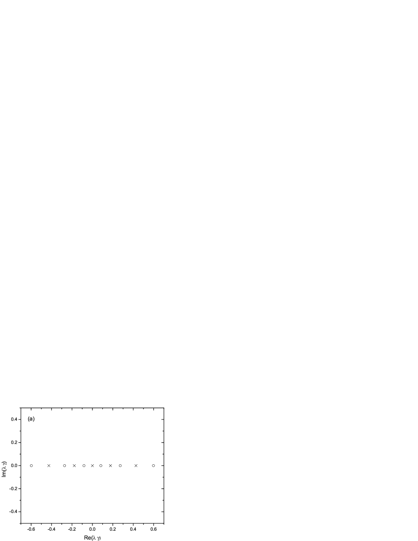
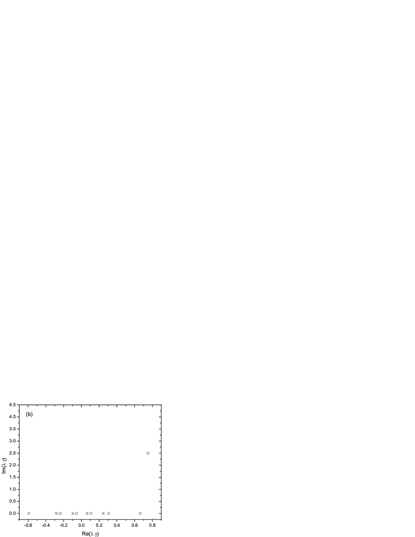
Figure 4: The Bethe ansatz roots $\lambda_{j}^{(+)}$ ($\circ$) and $\lambda_{j}^{(-)}$ ($\times$) for $\gamma=\frac{\pi}{5}$ and $L=12$. The roots refer to the dimensions (a) $X_{0,1}^{0,0}(\gamma)$ and (b) $X_{0,1}^{0,1}(\gamma)$.

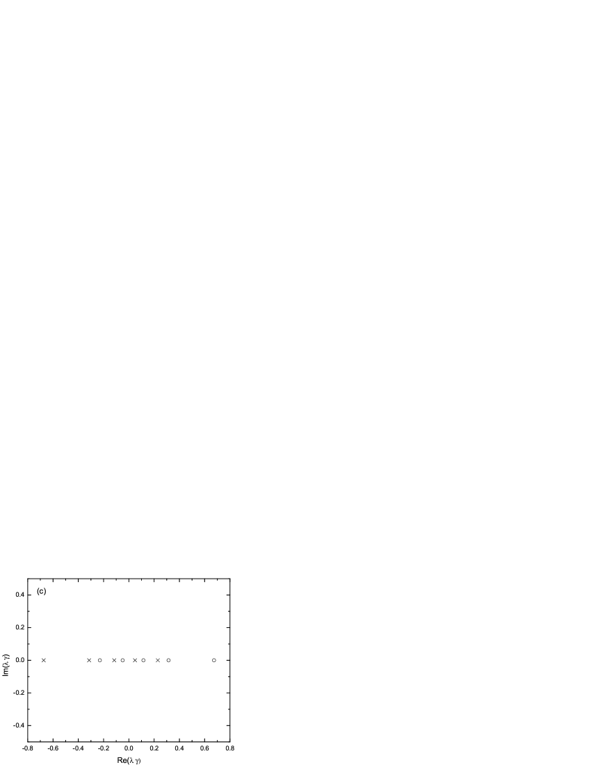
Figure 5: The Bethe ansatz roots $\lambda_{j}^{(+)}$ ($\circ$) and $\lambda_{j}^{(-)}$ ($\times$) for $\gamma=\frac{\pi}{5}$ and $L=12$. The roots refer to the dimensions (a) $X_{0,0}^{\frac{1}{2},\frac{1}{2}}(\gamma)$ , (b) $X_{1,1}^{\frac{1}{2},\frac{1}{2}}(\gamma)$ and $X_{1,1}^{\frac{1}{2},-\frac{1}{2}}$.

References

[1] R.J. Baxter, “Exactly Solved Models in Statistical Mechanics”, Academic Press, New York, 1982.
[4] H.J. de Vega, J.Phys.A:Math. Gen. 21 (1988) L1089;
H.J. de Vega and E. Lopes, Nucl.Phys.B 362 (1991) 261.
[5] J. Suzuki, J.Phys.A:Math. Gen. 21 (1988) L1175.
[6] A. Kuniba, Nucl.Phys.B 389 (1993) 209.
[7] V. Knizhnik and A.B. Zamolodchikov, Nucl.Phys.B 247 (1984) 83.
[8] M.J. Martins, Nucl.Phys.B 636 (2002) 583.
[9] H.J. de Vega and E. Lopes, Phys.Rev.Lett. 67 (1991) 489.
[10] J. Suzuki, J.Phys.A: Math.Gen. 25 (1992) 1769.
[11] H. Saleur, Nucl.Phys.B 578 (2000) 552;
F.H.L. Essler, H. Frahm and H. Saleur, Nucl.Phys.B 712 (2005) 513.
[12] M.J. Martins, B. Nienhuis and R. Rietman, Phys.Rev.Lett. 81 (1998) 504.
[13] H. Frahm, Nucl.Phys.B 559 (1999) 613.
[14] J.L. Jacobsen and H. Saleur, Nucl.Phys.B 716 (2005) 439.
[15] J.L. Cardy, “Phase transitions and critical phenomena, vol 11,
Ed. C. Domb and J.L. Lebowitz, New York Academic, 1987.
[16] W. Galleas and M.J. Martins, Nucl.Phys.B 699 (2004) 455.
[17] W. Galleas and M.J. Martins, Nucl.Phys.B 732 (2006) 444.
[18] K.A. Dancer, M.D. Gould and J. Links, J.Stat.Mech.Theor.Exp. P06011 (2006).
[19] P.P. Kulish, J.Sov.Math. 35 (1986) 2648.
[20] M. Scheunert, QA/0004032.
[21] L.D. Faddeev, N. Yu Reshetkhin e L.A. Takhtajan,
Leningrad Math.J. 1 (1990) 193.
[22] T. Deguchi, A. Fujii and K. Ito, Phys,.Lett.B 238 (1990) 242; M.D. Gould,
J.R. Links, Y.Z. Zhang and I. Tsohantjis, J.Phys.A:Math.Gen. 30 (1997) 4313.
[23] A.J. Bracken, G.W. Delius, M.D. Gould and Y.-Z. Zhang, J.Phys.A:Math.Gen. 27 (1994) 6551;
Z. Maassarani, J.Phys.A:Math.Gen. 28 (1995) 1305.
[24] V.E. Korepin, G. Izergin and N.M. Bogoliubov, Quantum Inverse Scattering Method, Correlation
Functions and Algebraic Bethe Ansatz, Cambridge University Press, Cambridge, 1992.
[25] F.H.L. Essler and V.E. Korepin, Phys.Rev.B 46 (1992) 9147; A. Foerster and M. Karowski,
Nucl.Phys.B 396 (1993) 611; F.H.L. Essler, V.E.Korepin and K. Schoutens, Int.J.Mod.Phys.B 8 (1994) 3205.
[26]
F. Gohmann and A. Seel, J.Phys.A:Math.Gen. 37 (2004) 2843; G.A.P. Ribeiro and M.J. Martins, Nucl.Phys.B
738 (2006) 391.
[27] M.J. Martins and P.B. Ramos, Nucl. Phys. B 500 (1997) 579.
[28] H.J. de Vega and F. Woynarovich, Nucl. Phys. B 251 (1985) 434;
F. Woynarovich and H.-P. Eckle, J. Phys. A: Math. Gen. 20 (1987) L443.
[29] C.J. Hamer, G.R.W. Quispel and M.T. Batchelor, J. Phys. A 20
(1987) 5677; H. Frahm and V. Korepin, Phys. Rev. B 42 (1990) 10533.
[30] P. Ginsparg, Applied Conformal Field Theory, Les Houches, session XLIX, 1988,
Elsevier Science Publishers.
[31] H. Saleur and B.W. Kaufmann, Nucl.Phys.B 628 (2002) 407;
J.L. Jacobsen, N. Read and H. Saleur, Phys.Rev.Lett. 90 (2003) 090601.
[34] S.O. Warnaar and B. Nienhuis, J.Phys.A:Math.Gen. 26 (1993) 2301.
[35] T. Koma, Prog.Theor.Phys. 78 (1987) 1213; J. Suzuki, Y. Akutsu and M. Wadati, J.Phys.Soc. Japan
59 (1990) 2667; A. Klümper, Ann.Physik 1 (1992) 540; G. Juttner, A. Klümper and J. Suzuki, Nucl.Phys.B 512
(1998) 581.
[36] A. Klümper, M.T. Batchelor and P.A. Pearce, J.Phys.A 24 (1991) 3111;
C. Destri and H.J. de Vega, Nucl.Phys.B 438 (1995) 413.
[37] Z. Bassi and A. Leclair, Nucl.Phys.B 578 (2000) 577.