$p$-adic Inflation

Abstract:

We construct approximate inflationary solutions rolling away from the unstable maximum of $p$-adic string theory, a nonlocal theory with derivatives of all orders. Novel features include the existence of slow-roll solutions even when the slow-roll parameters, as usually defined, are much greater than unity, as well as the need for the Hubble parameter to exceed the string mass scale $m_{s}$. We show that the theory can be compatible with CMB observations if $g_{s}/\sqrt{p}\sim 10^{-7}$, where $g_{s}$ is the string coupling, and if $m_{s}<10^{-6}M_{p}$. A red-tilted spectrum is predicted, and the scalar-to-tensor ratio is bounded from above as $r<0.006$. The $p$-adic theory is shown to have identical inflationary predictions to a local theory with superPlanckian parameter values, but with the advantage that the $p$-adic theory is ultraviolet complete.

1 Introduction

Many string theorists and cosmologists have turned their attention to building and testing stringy models of inflation in recent years. The goals have been to find natural realizations of inflation within string theory, and novel features which would help to distinguish the string-based models from their more conventional field theory counterparts. The more popular categories include brane-antibrane [1], D3/D7 [2], modular [3], DBI [4] and tachyon-driven [5] inflation (see [6] for a review).

In most examples to date, string theory has been used to derive an effective 4D field theory operating at energies below the string scale. Since string theory provides a complete description of dynamics also at higher energies, it may be interesting to consider a model which takes advantage of this distinctive feature. This is usually daunting since the field theory description should be supplemented by an infinite number of higher dimensional operators at energies above the string scale, whose detailed form is not known. In the present work, we propose to take a small step in the direction of overcoming this barrier, by considering a simplified model of string theory invented in 1987 [7], in which the world-sheet coordinates of the string are restricted to the field of $p$-adic numbers. Scattering amplitudes of open string theory can be related to those of the $p$-adic strings. A great advantage in $p$-adic string theory is that it is possible to compute all amplitudes of its lowest state and to determine a simple field-theoretic Lagrangian which exactly reproduces them. The result is a nonlocal field theory which is nevertheless sensible in the far ultraviolet.

The $p$-adic string resembles the bosonic string in that its ground state is a tachyon, whose unstable maximum presumably indicates the presence of a decaying brane, analogous to the unstable D25-brane of the open bosonic string theory [8]. Similarly to the bosonic string, the potential is asymmetric around the maximum, with one direction leading to a zero-energy vacuum, while in the other direction the potential is unbounded from below. We will consider whether it is possible to get successful inflation from rolling toward the bounded direction. This has been tried before in the context of the open string tachyon, and is difficult [9] because the tachyon potential is not flat enough to give a significant period of inflation, and there are no parameters within the theory which can tune the potential to be more flat. In contrast, we will show that the $p$-adic string tachyon can roll slowly enough to give many e-foldings of inflation. There are two distinct regions of parameter space which allow for successful inflation. There is a region with $p=\mathcal{O}(1)$ for which the $p$-adic field potential is flat and slow roll inflation proceeds in the usual manner. However, there is also a region of parameter space with $p\gg 1$ for which the potential is extremely steep ($|\eta|=M_{p}^{2}|V^{\prime\prime}/V|$ may be as large as $10^{11}$) but the $p$-adic scalar field nevertheless rolls slowly. This remarkable behaviour relies on the nonlocal nature of the theory: the effect of the higher derivative terms in the action is to slow down the field sufficiently, despite its steep potential. This new effect manifests itself only in the regime where the higher derivative interactions cannot be ignored. It is also interesting that in our model the kinetic energy is responsible for driving inflation for a significant number of e-foldings, unlike in conventional models of inflation.

One may worry about the presence of these higher derivative terms, because they are usually known to introduce ghosts into the theory. In fact, it is easy to check that for a scalar field theory if one introduces only a finite number of higher derivatives, then the model invariably contains ghost degrees of freedom. The reason why the $p$-adic string action can evade this problem is because it is intrinsically nonperturbative in nature, the propagator being modified in such a way as to not contain any poles. In other words there are no physical states, ghosts or otherwise, around the true vacuum. This novel way of curing the problem of ghosts in higher derivative theories, while retaining some nice properties such as improved UV behaviour, was already pointed out in [12] in the context of gravity. It was also pointed out in [12] that such theories can exibit interesting new cosmological features. For instance, one can obtain nonsingular bouncing solutions by making gravity weak at short distances. More recently, such models have also been shown to possess inflationary solutions [13]. However, the models of [12, 13] are phenomenological, while the $p$-adic action that we consider is an actual (albeit exotic) string theory and reproduces many nontrivial features of conventional string theories.

We start by reviewing the salient features of $p$-adic string theory in section 2. In section 3 we show that this theory does not give inflation if the higher-derivative terms in the action are ignored. However, near the top of the potential, the energy can be large enough to justify keeping all higher derivative terms. In section 4 we show how to resum their contributions and we construct approximate inflationary solutions valid near the top of the potential, by solving the coupled equations for the tachyon and scale factor of the universe. We give two different approximate methods in this section. In section 5 we solve for the fluctuations around this background to determine the power spectrum of scalar and tensor perturbations which can be probed by the cosmic microwave background (CMB). There we show that it is possible to choose parameters which are compatible with the measured amplitude and spectral index, and that the scalar-to-tensor ratio is bounded from above as $r<0.006$ in this model. We also argue that it can be natural to have initial conditions compatible with inflation in the $p$-adic theory. We give conclusions in section 6. Appendix A gives details about the $p$-adic stress tensor and the approximate inflationary solution of the Friedmann equation. Appendix B gives mathematical details about the incomplete cylindrical functions of the Sonine-Schaefli form. Appendix C explains a formal equivalence between the dynamics of the $p$-adic tachyon and those of a local field theory with a super-Planckian vacuum expectation value (VEV).

2 Review of $p$-adic string theory

The action of $p$-adic string theory is given by [7]

$$S = {m_{s}^{4}\over g_{p}^{2}}\int d^{\,4}x\ \left(-\frac{1}{2}\phi\,p^{-{\Box\over 2m_{s}^{2}}}\phi+{1\over p+1}\phi^{p+1}\right)$$ (1)

$$\equiv {m_{s}^{4}\over g_{p}^{2}}\int d^{\,4}x\ \left(-\frac{1}{2}\phi\,e^{-{\Box\over m_{p}^{2}}}\phi+{1\over p+1}\phi^{p+1}\right)$$

where $\Box=-\partial_{t}^{2}+\nabla^{2}$ in flat space and we have defined

$${1\over g_{p}^{2}}\equiv{1\over g_{s}^{2}}{p^{2}\over p-1}\mbox{ and }m_{p}^{2}\equiv{2m_{s}^{2}\over\ln p}$$ (2)

The dimensionless scalar field $\phi(x)$ describes the open string tachyon, $m_{s}$ is the string mass scale and $g_{s}$ is the open string coupling constant. Though the action (1) was originally derived for $p$ a prime number, it appears that it can be continued to any postive integer and even makes sense in the limit $p\rightarrow 1$ [14]. Setting $\Box=0$ in the action, the resulting potential takes the form $V=(m_{s}^{4}/g_{p}^{2})(\frac{1}{2}\phi^{2}-\frac{1}{p+1}\phi^{p+1})$. Its shape is shown in figure 1.

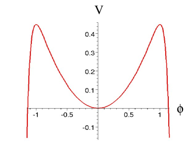
Figure 1: The potential of the $p$-adic tachyon for $p=19$.

The action (1) is a simplified model of the bosonic string which only qualitatively reproduces some aspects of a more realistic theory. That being said, there are several nontrivial similarities between $p$-adic string theory and the full string theory. For example, near the true vacuum of the theory $\phi=0$ the field naively has no particle-like excitations since its mass squared goes to infinity.  This is the $p$-adic version of the statement that there are no open string excitations at the tachyon vacuum. A second similarity is the existence of lump-like soliton solutions representing $p$-adic D-branes [15]. The theory of small fluctuations about these lump solutions has a spectrum of equally spaced masses squared for the modes [15],[16], as in the case of normal bosonic string theory.

It should also be noted that the connection between (1) and the DBI-type tachyon actions, which have been widely studied in the literature in the context of tachyon matter [17], is not entirely clear (see [18] for a discussion of the relation between $p$-adic and ordinary strings). In the case of tachyon matter, solutions which roll towards the vacuum $T\rightarrow\infty$ have late time asymptotics $T\sim t$ and hence the tachyon never reaches this point [19], whereas in the case of the $p$-adic string the vacuum is at a finite point in the field configuration space and homogeneous solutions rolling towards the vacuum typically pass this point without difficulty [11] (at least in flat space). In fact, the numerical studies of [11] found no homogeneous solutions which appeared to correspond to tachyon matter (vanishing pressure at late times). This issue has been considered in the case of cubic string field theory in [20]. Related rolling tachyon solutions in cubic string field theory have been discussed in [21].

It is worth pointing out that one obtains very similar actions to (1) with exponential kinetic operators (and usually assumed to have a cubic or quartic potential) when quantizing strings on random lattice [22]. These field theories are also known to reproduce several features, such as the Regge behaviour [23], of their stringy duals. Although our analysis focuses on the specific $p$-adic action, it can easily be applied to such theories as well. The connection between $p$-adic string theory and ordinary string theory on a discrete lattice was explored in [18].

The field equation that results from (1) is

$$e^{-{\Box/m_{p}^{2}}}\,\phi=\phi^{p}$$ (3)

We are interested in perturbing around the solution $\phi=1$, which is a critical point of the potential, representing the unstable tachyonic maximum. For odd $p$ one also has another unstable point at $\phi=-1$, but we will restrict our attention to solutions that start to evolve from the omnipresent $\phi=1$ maximum. In passing we also note that there is also the stable vacuum of the tachyon, at $\phi=0$. For both even and odd $p$ the potential is unbounded from below.

It is also worth commenting on the physical interpretation of the fact that the potential is unbounded from below. The instability associated with the decay of the “closed string vacuum” $\phi=0$ to the “true vacuum” $\phi=\infty$ is thought to be associated with the closed string tachyon instability [8].

Notice that in the limit $p\rightarrow 1$ the equation of motion (3) becomes a local equation

$$\Box\phi=2\phi\ln\phi$$

Therefore $p\rightarrow 1$ is the limit of local field theory. In the present work we will also consider a very different limit, $p\gg 1$, in which the nonlocal structure of (1) is playing an important role in the dynamics.

3 Absence of Naive Slow Roll Dynamics

One may wonder whether the field theory (1) naively allows for slow roll inflation in the conventional sense. Naively one might expect that for a slowly rolling field the higher powers of $\Box$ in the kinetic term are irrelevant and one may approximate (1) by a local field theory. The action (1) can be rewritten as

$$S=\int d^{4}x\left[\frac{1}{2}\chi\Box\chi-V(\chi)+\cdots\right]$$ (4)

where we have defined the field $\chi$ as

$$\chi = \chi_{0}\,\phi$$ (5)

$$\chi_{0} = \frac{p}{g_{s}}\sqrt{\frac{\ln p}{2(p-1)}}\,m_{s}$$ (6)

and the potential is

$$V(\chi)=\frac{m_{s}^{2}}{\ln p}\chi^{2}-\frac{m_{s}^{4}}{g_{s}^{2}}\frac{p^{2}}{p^{2}-1}\left(\frac{\chi}{\chi_{0}}\right)^{p+1}$$ (7)

In (4) the $\cdots$ denotes terms with higher powers of $\Box$. The truncation (4) is quite analogous to what is usually performed in the literature when one studies inflation from the string theory tachyon [5]. In the case of the usual string theory tachyon corrections involving $\Box^{2}$ and higher are expected, but the full infinite series of higher derivative terms is not known explicitly (see, however, [25] for a calculation of the string theory tachyon action up to order $\partial^{6}$). Thus, the standard approach is to simply neglect such terms. We will show, however, that under certain circumstances the higher derivative corrections may play an extremely important role in the inflationary dynamics.

Working in the context of the action (4) let us consider the slow roll parameters describing the flatness of the potential (7) about the unstable maximum $\chi=\chi_{0}$. It is straightforward to show that

$$\left.\frac{M_{p}^{2}}{2}\frac{1}{V(\chi_{0})^{2}}\left(\frac{\partial V(\chi)}{\partial\chi}\right)^{2}\right|_{\chi=\chi_{0}} = 0$$ (8)

$$\left.M_{p}^{2}\frac{1}{V(\chi_{0})}\frac{\partial^{2}V(\chi)}{\partial\chi^{2}}\right|_{\chi=\chi_{0}} = -\frac{4g_{s}^{2}}{\ln p}\frac{p^{2}-1}{p^{2}}\left(\frac{M_{p}}{m_{s}}\right)^{2}$$ (9)

Thus one would naively expect that inflation is only possible in the theory (1) for $g_{s}M_{p}/(\sqrt{\ln p}\,m_{s})$ $\ll 1$. For $p=\mathcal{O}(1)$ we will see that this expectation is correct, however, for $p\gg 1$ this intuition is incorrect and that successful inflation can occur even with $M_{p}^{2}V^{-1}\partial^{2}V/\partial\chi^{2}\sim-10^{16}\,$! The reason for this surprising result is that the dynamics of the $p$-adic tachyon field is set by the mass scale which appears in the kinetic term, $m_{s}$, rather than the mass scale which is naively implied by the potential

$$m_{\chi}^{2}(\chi_{0})\equiv\left.\frac{\partial^{2}V}{\partial\chi^{2}}\right|_{\chi=\chi_{0}}=-\frac{2(p-1)}{\ln p}m_{s}^{2}$$ (10)

Clearly for $p\gg 1$ we have $|m_{\chi}^{2}|\gg m_{s}^{2}$.

4 Approximate Solutions: Analytical techniques

In this section we construct the approximate solutions for the scalar field and the quasi-de Sitter expansion of the universe, in which $\phi$ starts near the unstable maximum ($\phi=1$) of its potential and rolls slowly toward the minimum ($\phi=0$). Cosmological solutions of similar nonlocal theories have also been considered in [24].

We use two different formalisms to construct inflationary solutions. We first devise a perturbative expansion in $e^{\lambda t}$ similar to what was carried out in [11] to study rolling solutions in flat spacetime. Our second formalism is the analogue of the usual slow roll approximation: we assume that the friction term in the $\Box$ operator dominates over the acceleration term and also neglect the time variation of $H$.

We first discuss the perturbative expansion in powers of $e^{\lambda t}$. Our starting point is the ansatz

$$\phi(t)=1-\sum_{r=1}^{\infty}\phi_{r}e^{r\lambda t}$$ (11)

and

$$H(t)=H_{0}-\sum_{r=1}^{\infty}H_{r}e^{r\lambda t}$$ (12)

We have chosen the parameterisation such that at $t\rightarrow-\infty$, $\phi$ starts from the top of the hill where the universe is undergoing de Sitter expansion with Hubble constant $H_{0}$. As $t\rightarrow-\infty$, $e^{\lambda t}\rightarrow 0$ and all the correction terms, which quantify the departure from the pure de Sitter phase, vanish. As $t$ increases, the field rolls toward the true vacuum $\phi=0$, in fact reaching it at a finite time. Classically, the model admits infinitely many e-foldings of inflation, although only the last 60 e-foldings before the end of inflation are relevant for observation. This idealized behaviour is an artifact of neglecting quantum fluctuations; quantum mechanically the field cannot sit at $\phi=1$ for an infinite amount of time. We will return to this issue later and show that the inclusion of quantum fluctuations does not spoil inflation, which it would in ordinary local field theory if the $\eta$ parameter is large.

Given the ansatz (11,12), we can expand the field equation for the $p$-adic scalar (3) and the Friedmann equation as a series in $e^{\lambda t}$ and then determine the coefficients $\{\phi_{r},H_{r}\}$ systematically, order by order. We will show that this can be done consistently. The zeroth order Klein-Gordon equation is trivially satisfied, by virtue of the fact that we start from a maximum of the potential.

4.1 $p$-adic Scalar Field Evolution

Let us first find an approximate solution for the scalar field equation of motion (3). We note that to compute quantities such as $\Box^{n}e^{\lambda t}$ to the order of interest, it is sufficient to use a truncation of (11) and (12):

$$\phi=1-u-\phi_{2}u^{2},\qquad H=H_{0}-H_{1}u-H_{2}u^{2}$$ (13)

where we have used the freedom to choose the origin of time to set $\phi_{1}\equiv 1$, and for convenience we have defined the new variable

$$u\equiv e^{\lambda t}$$ (14)

in terms of which the $\Box$ operator takes the form

$$\Box=-\lambda^{2}\left[u^{2}{\partial^{2}\over\partial u^{2}}+\left(1+{3H\over\lambda}\right)u\,{\partial\over\partial u}\right]$$ (15)

We wish to compute quantities such a $\Box^{n}e^{\lambda t}$ up to ${\cal O}(u^{2})$. This can be done recursively. Writing $\Box^{n}\phi$ (where $n\geq 1$) as

$$(-\Box)^{n}\phi=A_{n}u+B_{n}u^{2}+\dots$$ (16)

and applying another $\Box$ operator one finds the following recursion relations for the coefficients $A_{n}$ and $B_{n}$:

$$A_{n+1}=A_{n}(\lambda^{2}+3H_{0}\lambda)$$ (17)

and

$$B_{n+1}=B_{n}(4\lambda^{2}+6H_{0}\lambda)-3H_{1}\lambda A_{n}$$ (18)

Equation (17) has the solution

$$A_{n}=a_{1}\left(\lambda^{2}+3H_{0}\lambda\right)^{n}$$ (19)

with $a_{1}=-1$ (from examination of $\Box\phi$) while a suitable ansatz for $B_{n}$ is given by

$$B_{n}=b_{1}(\lambda^{2}+3H_{0}\lambda)^{n}+b_{2}(4\lambda^{2}+6H_{0}\lambda)^{n}$$ (20)

The coefficients $b_{1},b_{2}$ can be deduced from (18) using the initial values

$$b_{1}=-{H_{1}\over H_{0}+\lambda}\mbox{ and }\ b_{2}={H_{1}\over H_{0}+\lambda}-\phi_{2}$$ (21)

which follow from explicitly computing $\Box\phi$ and $\Box^{2}\phi$. Putting everything together we now have

$$(-\Box)^{n}\phi = \delta_{n,0}-(\lambda^{2}+3H_{0}\lambda)^{n}u+\left[\left({H_{1}\over H_{0}+\lambda}-\phi_{2}\right)(4\lambda^{2}+6H_{0}\lambda)^{n}\right.$$ (22)

$$\left.-{H_{1}\over H_{0}+\lambda}(\lambda^{2}+3H_{0}\lambda)^{n}\right]u^{2}+\mathcal{O}(u^{3})$$

which works also for the case $n=0$. Using (22) one can resum the contributions coming from all the powers of $\Box$ in the exponential operator $e^{-\Box/m_{p}^{2}}$ to give

$$e^{-{\Box/m^{2}_{p}}}\,\phi=1-e^{\mu_{1}}u+\left[\left(\sigma-\phi_{2}\right)e^{\mu_{2}}-\sigma e^{\mu_{1}}\right]u^{2}+\cdots$$ (23)

where we have introduced

$$\mu_{1}\equiv{\lambda^{2}+3H_{0}\lambda\over m_{p}^{2}}\ \mbox{ , }\ \mu_{2}\equiv{4\lambda^{2}+6H_{0}\lambda\over m_{p}^{2}}\ \mbox{ and }\ \sigma\equiv{H_{1}\over H_{0}+\lambda}$$ (24)

We conjecture that such resummations are possible for higher order terms as well. Notice that (23) reduces to $\phi$ in the limit $m_{p}\to\infty$, as it should.

To solve the equation of motion for the scalar field, we must equate (23) to the right-hand-side of (3):

$$\phi^{p}=[1-u-\phi_{2}u^{2}]^{p}=1-pu-p\left(\phi_{2}-{p-1\over 2}\right)u^{2}+\cdots$$ (25)

matching coefficients for each order in $u$. The zeroth order equation is identically satisfied, as promised earlier, while matching at first order gives

$$e^{\mu_{1}}=e^{(\lambda^{2}+3H_{0})/m^{2}_{p}}=p$$ (26)

which, using (2) can be rewritten in the form

$$\lambda^{2}+3H_{0}\lambda=2m_{s}^{2}$$ (27)

which is independent of $p$. Later we will see that $H_{0}\gg m_{s}$ is necessary for getting inflation, so the solution of (27) is approximately

$$\lambda\cong{2m_{s}^{2}\over 3H_{0}}$$ (28)

Finally, matching coefficients at second order gives

$$\sigma e^{\mu_{1}}+\left(\phi_{2}-\sigma\right)e^{\mu_{2}}=p\left(\phi_{2}-{p-1\over 2}\right)$$ (29)

In summary, by solving the scalar field equation of motion (3) to second order in the expansion in powers of $u=e^{\lambda t}$, we have obtained two relations, (27) and (29). The former determines the parameter $\lambda$ while the latter determines $\phi_{2}$.

4.2 The Stress Energy Tensor and the Friedmann Equation

To complete our approximate solution for the classical background, we must solve the Friedmann equation

$$H^{2}={1\over 3M_{p}^{2}}\,\rho_{\phi}$$ (30)

to second order in $u$. To find the energy density $\rho_{\phi}$, we turn to the stress energy tensor for the $p$-adic scalar field. A convenient expression for $T_{\mu\nu}$ was derived in [26] (see also [27])

$$T_{\mu\nu}={m_{s}^{4}\over 2g_{p}^{2}}g_{\mu\nu}\left[\phi e^{-{\Box\over m_{p}^{2}}}\phi-{2\over p+1}\phi^{p+1}+{1\over m_{p}^{2}}\int_{0}^{1}d\tau\ \left(\Box e^{-{\tau\Box\over m_{p}^{2}}}\phi\right)\left(e^{-{(1-\tau)\Box\over m_{p}^{2}}}\phi\right)\right.$$ (31)

$$\left.+{1\over m_{p}^{2}}\int_{0}^{1}d\tau\ \left(\partial_{\alpha}e^{-{\tau\Box\over m_{p}^{2}}}\phi\right)\left(\partial^{\alpha}e^{-{(1-\tau)\Box\over m_{p}^{2}}}\phi\right)\right]-{m_{s}^{4}\over m_{p}^{2}g_{p}^{2}}\int_{0}^{1}d\tau\ \left(\partial_{\mu}e^{-{\tau\Box\over m_{p}^{2}}}\phi\right)\left(\partial_{\nu}e^{-{(1-\tau)\Box\over m_{p}^{2}}}\phi\right)$$

One may verify that the $T_{\mu\nu}$ is symmetric by changing the dummy integration variable $\tau\rightarrow 1-\tau$ in the last term. For homogeneous $\phi(t)$ the above expression simplifies, and for $T_{00}$ we find

$$\rho_{\phi}=-T_{00}={m_{s}^{4}\over 2g_{p}^{2}}\left[\phi e^{-{\Box\over m_{p}^{2}}}\phi-{2\over p+1}\phi^{p+1}+{1\over m_{p}^{2}}\int_{0}^{1}d\tau\ \left(\Box e^{-{\tau\Box\over m_{p}^{2}}}\phi\right)\left(e^{-{(1-\tau)\Box\over m_{p}^{2}}}\phi\right)\right.$$

$$\left.+{1\over m_{p}^{2}}\int_{0}^{1}d\tau\ \partial_{t}\left(e^{-{\tau\Box\over m_{p}^{2}}}\phi\right)\partial_{t}\left(e^{-{(1-\tau)\Box\over m_{p}^{2}}}\phi\right)\right]$$ (32)

One can evaluate the above expression term by term, keeping up to ${\cal O}(e^{2\lambda t})\sim u^{2}$. The final result reads

$$T_{00} = {m_{s}^{4}\over 2g_{p}^{2}}\left[1-u(1+e^{\mu_{1}})-{2[1-(p+1)u]\over p+1}+u(e^{\mu_{1}}-1)\right]+{\cal O}(u^{2})$$ (33)

$$= {m_{s}^{4}(p-1)\over 2g_{p}^{2}(p+1)}+{\cal O}(u^{2})$$

The ${\cal O}(u)$ terms cancel out and matching the coefficients in the Friedmann equation gives us the simple results

$$H_{0}^{2}={m_{s}^{4}\over 6M_{p}^{2}}{p-1\over g_{p}^{2}(p+1)}$$ (34)

and

$$H_{1}=0$$ (35)

for zeroth and first order respectively.

The ${\cal O}(u^{2})$ contribution to $T_{00}$ is quite complicated (see appendix A) but once we use (35) it simplifies greatly. Matching coefficient at order ${\cal O}(u^{2})$ in the Friedmann equation gives

$$H_{2}={\lambda m_{s}^{4}\over 4g_{p}^{2}m_{p}^{2}\,M_{p}^{2}}\,e^{\mu_{1}}=\frac{1}{8g_{s}^{2}}\frac{p^{3}\ln p}{p-1}\left(\frac{m_{s}}{M_{p}}\right)^{2}\lambda$$ (36)

Because of our sign convention for $H_{r}$, the fact that $H_{2}>0$ means that the expansion is slowing as $\phi$ rolls from the unstable maximum, as one would expect in a conventional inflationary model.

Using (28), (34) and (36) to compute $H_{2}/H_{0}\sim p\ln p$ it is clear that the perturbative expansion in $u$ breaks down once $u\sim(p\ln p)^{-1/2}$ (recall that $H\cong H_{0}-H_{2}u^{2}$). Thus one expects that once $u\sim p^{-1/2}$ then inflation ends. We verify this claim using an alternative formalism in the next subsection.

To summarize, we have determined the five parameters $\lambda,\phi_{2},H_{0},H_{1}$ and $H_{2}$ which appear in the solutions for $\phi(t)$ and $H(t)$ up to ${\cal O}(u^{2})$ through the equations (27-29), (34-36). As a check of our result, we can take $H_{0}\ll m_{s}$ and compare it to the the Minkowski background solution that was found in [11]. For $H_{0}\ll m_{s}$ we see from (27) that

$$\lambda\cong\sqrt{2}m_{s}\left(1-{3H_{0}\over 2\sqrt{2}m_{s}}\right)$$ (37)

the first term corresponding to the known Minkowski result. We can also compute the coefficient $\phi_{2}$ in this limit from (29),

$$\phi_{2}\cong-{1\over 2(p^{2}+p+1)}$$ (38)

This too coincides with the coefficient that was determined in [11] for $p=2$.

4.3 The Friction-Dominated Approximation

In the previous subsections we have constructed an approximate solution for the $p$-adic scalar rolling down its potential by performing an expansion of $\phi$, $H$ in a power series in $u$. Furthermore, we have shown that once $u\sim p^{-1/2}$ then this solution breaks down (because the $\mathcal{O}(u^{2})$ term in $H(t)$ become larger than the zeroth order term, $H_{0}$). At this point inflation has ended. Because the equations of motion are complicated, we now verify this behaviour using an alternative formalism which does not rely on small $u$.

The method is the same as the slow-roll approximation in ordinary inflation, which assumes that $\dot{\phi}\ll H\phi$. To justify it within the $p$-adic theory, we will provisionally assume that

$$\lambda^{2}\ll 3H_{0}\lambda$$

so that the evolution is friction-dominated in the usual sense. The consistency of this approximation will be established when we match the theory to the observables from the inflationary power spectrum later, in eqs. (70), (71). It follows that it is a good approximation to take

$$-\Box\cong 3H_{0}\partial_{t}$$

Then the $p$-adic scalar field equation becomes

$$e^{\alpha\partial_{t}}\phi=\phi^{p}$$ (39)

where we have defined

$$\alpha\equiv\frac{3H_{0}}{m_{p}^{2}}$$ (40)

Our procedure is to treat $H_{0}$ as exactly constant, solve for $\phi(t)$ and compute the energy density $\rho_{\phi}$. If $\rho_{\phi}$ is approximately constant then this series of approximations is self-consistent and the solution is reliable. Once $\rho_{\phi}$ begins to deviate significantly from a constant value then the solution breaks down and we conclude that inflation has ended.

We now proceed to solve (39) for constant $H_{0}$. To this end we expand $\phi(t)$ in Fourier modes as

$$\phi(t)=\frac{1}{\sqrt{2\pi}}\int_{-\infty}^{+\infty}dke^{-ikt}\phi_{k}$$ (41)

so that

$$e^{\alpha\partial_{t}}\phi(t) = \frac{e^{\alpha\partial_{t}}}{\sqrt{2\pi}}\int_{-\infty}^{+\infty}dke^{-ikt}\phi_{k}$$ (42)

$$= \frac{1}{\sqrt{2\pi}}\int_{-\infty}^{+\infty}dke^{-ik(t+\alpha)}\phi_{k}$$ (43)

$$= \phi(t+\alpha)$$ (44)

The $p$-adic scalar equation of motion (39) then takes the simple form

$$\phi(t+\alpha)=\phi(t)^{p}$$ (45)

It is quite remarkable that this equation admits dynamical solutions. It is straightforward to check that (45) has the solution

$$\phi(t)=e^{-u(t)}$$ (46)

where $u(t)=e^{\lambda t}$ and $\lambda=\alpha^{-1}\ln p=2m_{s}^{2}/(3H_{0})$, as before. One can easily check by acting on (46) with the full operator $-\Box=\partial_{t}^{2}+3H_{0}\partial_{t}$ that indeed the friction term dominates as long as $u\mbox{\raisebox{-2.58334pt}{~{}$\stackrel{{\scriptstyle<}}{{\sim}}$~{}}}1$.

Performing a Taylor expansion of (46) about $u=0$ gives

$$\phi\cong 1-u+\frac{1}{2}u^{2}+\cdots$$

which reproduces our solution in the small-$u$ expansion in the limit that $m_{s}\ll H_{0}$ (see equations 13 and 72). We also have

$$e^{-\Box/m_{p}^{2}}\phi=e^{-up}\cong 1-pu+\frac{1}{2}p^{2}u^{2}$$

which again reproduces our previous results (which can be verified by inserting the solutions for $\mu_{1}$, $\mu_{2}$, $\sigma$ and $\phi_{2}$ into equation 23).

We now proceed to construct the energy density for $\phi(t)$ in this approximation. It is straightforward to show that

$$e^{-\tau\Box/m_{p}^{2}}\phi = \exp\left(-up^{\tau}\right)$$

$$e^{-(1-\tau)\Box/m_{p}^{2}}\phi = \exp\left(-up^{1-\tau}\right)$$ (47)

We write $\rho_{\phi}$ (32) as

$$\rho_{\phi}\equiv\frac{m_{s}^{4}}{2g_{p}^{2}}\left[T_{1}+T_{2}+T_{3}+T_{4}\right]$$ (48)

where

$$T_{1} \equiv \phi e^{-\Box/m_{p}^{2}}\phi$$ (49)

$$T_{2} \equiv -\frac{2}{p+1}\phi^{p+1}$$ (50)

$$T_{3} \equiv \frac{1}{m_{p}^{2}}\int_{0}^{1}d\tau\left(\Box e^{-\frac{\tau\Box}{m_{p}^{2}}}\phi\right)\left(e^{-\frac{(1-\tau)\Box}{m_{p}^{2}}}\phi\right)$$ (51)

$$T_{4} \equiv \frac{1}{m_{p}^{2}}\int_{0}^{1}d\tau\partial_{t}\left(e^{-\frac{\tau\Box}{m_{p}^{2}}}\phi\right)\partial_{t}\left(e^{-\frac{(1-\tau)\Box}{m_{p}^{2}}}\phi\right)$$ (52)

Using the scalar field equation (3) and (46) the first two terms, (49) and (50), are trivial

$$T_{1}+T_{2}=\frac{p-1}{p+1}e^{-up-u}$$ (53)

Since this term is proportional to $\phi^{p+1}$ we identify it with the potential energy of the $p$-adic scalar.

The next simplest term to evaluate is $T_{4}$ (52) which gives

$$T_{4}=\frac{\lambda^{2}u^{2}}{2m_{s}^{2}}p\ln p\int_{0}^{1}d\tau\exp\left[-u\left(p^{\tau}+p^{1-\tau}\right)\right]$$

It is useful to change the variable of integration to $\omega=up^{\tau}$ and cast this result in the form

$$T_{4}=\frac{\lambda^{2}}{2m_{s}^{2}}(pu^{2})\int_{u}^{up}\frac{d\omega}{\omega}\exp\left[-\omega-\frac{pu^{2}}{\omega}\right]$$ (54)

The $d\omega$ integral can be performed exactly (though not in closed form) in terms of special functions. Since $T_{4}$ is subdominant to a contribution coming from $T_{3}$ we will not investigate the behaviour of (54) any further.

We now study $T_{3}$ (51). This can be written in the form

$$T_{3} = -\frac{\lambda^{2}}{2m_{s}^{2}}\int_{u}^{up}d\omega\omega\exp\left[-\omega-\frac{pu^{2}}{\omega}\right]$$ (55)

$$+ \frac{\lambda^{2}}{2m_{s}^{2}}\left(1+\frac{3H_{0}}{\lambda}\right)\int_{u}^{up}d\omega\exp\left[-\omega-\frac{pu^{2}}{\omega}\right]$$

The dominant contribution to $T_{3}$ is the one proportional to $H_{0}$ since the evolution is friction-dominated. This term is also larger than $T_{4}$. The leading contribution to $T_{3}+T_{4}$ is then

$$T_{3}+T_{4}\cong\int_{u}^{up}d\omega\exp\left[-\omega-\frac{pu^{2}}{\omega}\right]$$ (56)

where we have used the fact that $3H_{0}\lambda/(2m_{s}^{2})\cong 1$ which follows from (27) when $\lambda^{2}\ll 3H_{0}\lambda$. Since $T_{3}$ and $T_{4}$ contain time derivatives acting on $\phi$ it is natural to identify (56) with the kinetic energy of the $p$-adic scalar.

Let us study the behaviour of the kinetic energy, equation (56), as a function of $u$. The integral in (56) can be performed in terms of the incomplete cylindrical functions of the Sonine-Schlaefli form [32] (see appendix B for a review).

$$\int_{u}^{up}d\omega\exp\left[-\omega-\frac{pu^{2}}{\omega}\right]=2\pi up^{1/2}S_{-1}(-u,-up;2iup^{1/2})$$

We now study the behaviour of this integral in various limits. We assume that $p\gg 1$ throughout since the previous method of expanding in $u$ is valid in the case where $p\sim 1$. At very early times, $u<1/p$, this integral goes to zero as

$$\int_{u}^{up}d\omega\exp\left[-\omega-\frac{pu^{2}}{\omega}\right]\cong up\hskip 14.22636pt\mathrm{for}\hskip 14.22636ptu<1/p$$

For intermediate times, $1/p\ll u\mbox{\raisebox{-2.58334pt}{~{}$\stackrel{{\scriptstyle<}}{{\sim}}$~{}}}1/p^{1/2}$, it is a good approximation to treat the upper and lower limits of integration as $0$ and $+\infty$ respectively. In this approximation we can write the incomplete cylinder function in terms of a Hankel function of order $\nu=-1$ (see appendix B for details). The small argument asymptotics of $H_{-1}^{(1)}$ gives

$$\int_{u}^{up}d\omega\exp\left[-\omega-\frac{pu^{2}}{\omega}\right]\cong 1+2u^{2}p\ln(2up^{1/2})\hskip 14.22636pt\mathrm{for}\hskip 14.22636pt1/p\ll u<1/p^{1/2}$$

Finally we consider late times, $u>1/p^{1/2}$. It is still reasonable to extend the integral as $\int_{u}^{up}d\omega\cong\int_{0}^{\infty}d\omega$ and hence the integral can still be written in terms of $H_{-1}^{(1)}$. This time the large-argument asymptotics of the Hankel function are appropriate and one has

$$\int_{u}^{up}d\omega\exp\left[-\omega-\frac{pu^{2}}{\omega}\right]\cong\sqrt{\pi up^{1/2}}e^{-2up^{1/2}}\hskip 14.22636pt\mathrm{for}\hskip 14.22636ptu>1/p^{1/2}$$

We have verified these asymptotic expressions numerically.

We can now write the dominant contribution to $\rho_{\phi}$ in the friction-dominated approximation,

$$\rho_{\phi}=\frac{m_{s}^{4}}{2g_{s}^{2}}\frac{p^{2}}{p-1}\left(\frac{p-1}{p+1}e^{-up-u}+\int_{u}^{up}d\omega\exp\left[-\omega-\frac{pu^{2}}{\omega}\right]\right)$$ (57)

The first term, proportional to $e^{-up}$, represents the potential energy and the second term represents the kinetic energy. Using our previous analysis of the kinetic energy the behaviour of $\rho_{\phi}$ as a function of $u$ (assuming $p\gg 1$) is clear. At early times $u<1/p$ the potential energy dominates and we have $\rho_{\phi}\cong m_{s}^{4}/(2g_{p}^{2})$. At intermediate times $1/p\ll u\mbox{\raisebox{-2.58334pt}{~{}$\stackrel{{\scriptstyle<}}{{\sim}}$~{}}}1/p^{1/2}$ the potential energy goes to zero and the kinetic energy dominates and we have $\rho\cong m_{s}^{4}/(2g_{p}^{2})$. At late times $u>1/p^{1/2}$ and $\rho_{\phi}$ damps to zero as $e^{-2up^{1/2}}$. We have verified this behaviour numerically. Figure 2 shows the behaviour of $\rho_{\phi}$ as a function of $t$, verifying that $\rho_{\phi}$ is approximately constant for $u<p^{-1/2}$. The time evolution of both the potential energy and the kinetic energy contributions to $\rho_{\phi}$ are shown, demonstrating that the latter dominates in the interval $p^{-1}<u<p^{-1/2}$. In this figure we have taken $p=10^{5}$ for illustrative purposes.

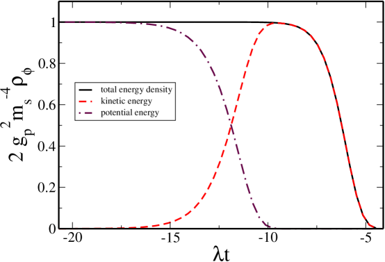
Figure 2: Plot of the energy density of the $p$-adic scalar as a function of $t$, for $p=10^{5}$. This figure shows that $\rho_{\phi}$ is approximately constant for $u<p^{-1/2}$. The individual contributions from the potential and kinetic energy are also shown.

We conclude that for $u\mbox{\raisebox{-2.58334pt}{~{}$\stackrel{{\scriptstyle<}}{{\sim}}$~{}}}1/p^{1/2}$ the scalar field energy density $\rho_{\phi}$ is approximately constant and inflation proceeds. At $u=1/p^{1/2}$ the energy density of the $p$-adic scalar begins to decrease quickly and the analysis of this subsection is no longer applicable. We conclude that inflation ends, roughly, when $u=1/p^{1/2}$.

It is quite interesting that during the intermediate phase $p^{-1}<u<p^{-1/2}$ it is in fact the kinetic energy which is driving inflation, rather than the potential energy. This is quite different from what occurs in a local field theory.

5 Fluctuations and Inflationary Predictions

In this section we consider the spectrum of cosmological fluctuations produced during $p$-adic inflation. The full cosmological perturbation theory for the $p$-adic string model (1), which should include metric perturbations and also take into account the departure of the background expansion from pure de Sitter, is complicated and beyond the scope of the present paper. We leave a detailed study of these matters to future investigation [37]. To simplify the analysis we will neglect scalar metric perturbations as well as deviations of the background metric from pure de Sitter space during horizon crossing. In standard cosmological perturbation theory these approximations reproduce the more exact results to reasonable accuracy and we therefore assume that the situation is similar for the action (1).

5.1 $p$-adic Tachyon Fluctuations

We are approximating the background dynamics as de Sitter which amounts to working in the limit $u\rightarrow 0$ so that

$$H^{2} \equiv H_{0}^{2}=\frac{m_{s}^{4}}{6M_{p}^{2}}\frac{p-1}{g_{p}^{2}(p+1)}$$ (58)

$$\phi \equiv \phi_{0}\equiv 1$$ (59)

We expand the $p$-adic tachyon field in perturbation theory as

$$\phi(t,\vec{x}) = \phi^{(0)}(t)+\delta\phi(t,\vec{x})$$

$$= 1+\delta\phi(t,\vec{x})$$

The perturbed Klein-Gordon equation (3) takes the form

$$e^{-\Box/m_{p}^{2}}\,\delta\phi=p\,\delta\phi$$ (60)

(Inhomogeneous solutions in $p$-adic string theory have also been considered in [28].) One can construct solutions by taking $\delta\phi$ to be an eigenfunction of the $\Box$ operator. If we choose $\delta\phi$ to satisfy

$$-\Box\delta\phi=+B\,\delta\phi$$ (61)

then this is also a solution to (60) if

$$B=m_{p}^{2}\ln p=2m_{s}^{2}$$ (62)

where in the second equality we have used (2).

The solutions of (61) are well known. However, in order to make contact with the usual treatment of cosmological perturbations we need to define a field in terms of which the action appears canonical. This presents a serious difficulty because, in general, there is no local field redefinition which will bring the kinetic term $\phi\left(1-e^{-\Box/m_{p}^{2}}\right)\phi$ into the canonical form $\phi\Box\phi$. (One might imagine simply truncating the expansion in powers of $\Box$ as we have described in section 3, however, the higher order terms are not negligible in general.) Fortunately, for fields which are on-shell (that is, when (61) is solved) the field obeys

$$\left(1-e^{-\Box/m_{p}^{2}}\right)\delta\phi = \left(1-e^{B/m_{p}^{2}}\right)\delta\phi$$

$$= \left(1-e^{B/m_{p}^{2}}\right)\frac{1}{(-B)}\,(-B)\delta\phi$$

$$= \left(1-e^{B/m_{p}^{2}}\right)\frac{1}{(-B)}\,\Box\delta\phi$$

$$= \frac{p-1}{2m_{s}^{2}}\,\Box\delta\phi$$

Thus, for on-shell fields the kinetic term in the Lagragian can be written as

$$\mathcal{L}_{\mathrm{on-shell}} = \frac{m_{s}^{4}}{g_{p}^{2}}\frac{1}{2}\phi(1-e^{-\Box/m_{p}^{2}})\phi+\cdots$$ (63)

$$= \frac{m_{s}^{4}}{g_{p}^{2}}\frac{p-1}{2m_{s}^{2}}\frac{1}{2}\phi\Box\phi+\cdots$$

$$= \frac{1}{2}\varphi\Box\varphi+\cdots$$

In (63) we have defined the “canonical” field

$$\varphi\equiv A\phi$$ (64)

where

$$A\equiv\frac{m_{s}p}{\sqrt{2}\,g_{s}}$$ (65)

The field $\varphi$ has a canonical kinetic term in the action, at least while (61) is satisfied. Notice that $\varphi$ is distinct from the field $\chi$ (see (5)) which we introduced in section 3. The field $\chi$ corresponds to the canonical field which one would naively define when neglecting terms $\mathcal{O}(\Box^{2})$ and higher in the action (as is typical in studies of tachyonic inflation) while $\varphi$ is the appropriate definition of the canonically normalized field when taking into account the infinite series of higher derivative corrections.

Now, let us return to the task of solving (61), bearing in mind that $\delta\varphi=A\delta\phi$ is the appropriate canonically normalized field. We write the quantum mechanical solution in term of annihilation/creation operators as

$$\delta\varphi(t,\vec{x})=\int\frac{d^{\,3}k}{(2\pi)^{3/2}}\left[a_{k}\varphi_{k}(t)e^{ikx}+\mathrm{h.c.}\right]$$

and the mode functions $\varphi_{k}(t)$ are given by

$$\varphi_{k}(t)=\frac{1}{2}\sqrt{\frac{\pi}{a^{3}H_{0}}}\,e^{\frac{i\pi}{2}\left(\nu+1/2\right)}\,H_{\nu}^{(1)}\!\left(\frac{k}{aH_{0}}\right)$$ (66)

where the order of the Hankel functions is

$$\nu=\sqrt{\frac{9}{4}+\frac{B}{H_{0}^{2}}}=\sqrt{\frac{9}{4}+\frac{2m_{s}^{2}}{H_{0}^{2}}}$$ (67)

and of course $a=e^{H_{0}t}$. In the second equality in (67) we have used (62) and (2). In writing (66) we have used the usual Bunch-Davies vacuum normalization so that on small scales, $k\gg aH_{0}$, one has

$$|\varphi_{k}|\cong\frac{a^{-1}}{\sqrt{2k}}$$

which reproduces the standard Minkowski space fluctuations. This is the usual procedure in cosmological perturbation theory. However, we note that the quantization of the theory (1) is not transparent and it might turn out that the usual prescription is incorrect in the present context. We defer this and other subtleties to future investigation. On large scales, $k\ll aH_{0}$, the solutions (66) behave as

$$|\varphi_{k}|\cong\frac{H}{\sqrt{2k^{3}}}\left(\frac{k}{aH_{0}}\right)^{3/2-\nu}$$

which gives a large-scale power spectrum for the fluctuations

$$P_{\delta\varphi}=\left(\frac{H_{0}}{2\pi}\right)^{2}\left(\frac{k}{aH_{0}}\right)^{n_{s}-1}$$

with spectral index

$$n_{s}-1=3-2\nu$$

From (67) it is clear that to get an almost scale-invariant spectrum we require $m_{s}\ll H_{0}$. In this limit we have

$$n_{s}-1\cong-\frac{4}{3}\left(\frac{m_{s}}{H_{0}}\right)^{2}$$ (68)

which gives a red tilt to the spectrum, in agreement with the latest WMAP data [29]. For $n_{s}\cong 0.95$ one has $m_{s}\cong 0.2H_{0}$. Comparing (66) to the corresponding solution in a local field theory we see that the $p$-adic tachyon field fluctuations evolve as though the mass-squared of the field was $-2m_{s}^{2}$ which may be quite different from the mass scale which one would infer by truncating the infinite series of derivatives: $\partial^{2}V/\partial\chi^{2}(\chi=\chi_{0})$ (see eq. (10)). The fact that $H_{0}>m_{s}$ is an unusual feature; we will comment on it below.

It is worth pointing out that we have constructed solutions of a partial differential equation with infinitely many derivatives, for which we are free to specify two initial data; to obtain eq. 66 we fixed these using the Bunch-Davies prescription. Precisely the same result was obtained when inhomogeneous solutions were studied in [28]. Partial differential equations with infinitely many derivatives constitute a new class of equations in mathematical physics about which little is presently known. In particular, it is not clear how to pose the intial value problem for such equations. We conjecture that the most general solutions of (3) are specified by two initial data (for example $\phi(0,\vec{x})$ and $\dot{\phi}(0,\vec{x})$), just like equations containing only one power of $\Box$. See [30] for mathematical work on constructing solutions of equations with infinitely many derivatives.

5.2 Determining Parameters

We now want to fix the parameters of the model by comparing to the observed features of the CMB perturbation spectrum. There are three dimensionless parameters, $g_{s},\ p$ and the ratio $m_{s}/M_{p}$. The important question is whether there is a sensible parameter range which can account for CMB observations, i.e., the spectral tilt and the amplitude of fluctuations. Using (34) in (68), we can relate the tilt to the model parameters via

$$|n_{s}-1|=\frac{8(p+1)}{p^{2}}\left(\frac{M_{p}}{m_{s}}\right)^{2}g_{s}^{2}\quad\Longleftrightarrow\quad\left(\frac{m_{s}}{M_{p}}\right)^{2}=\frac{8(p+1)}{p^{2}}\frac{g_{s}^{2}}{|n_{s}-1|}$$ (69)

Thus one can have a small tilt while ensuring that the string scale is smaller than the Planck scale, provided that $g_{s}^{2}/p\ll 1$. Henceforth we will use (69) to determine $m_{s}/M_{p}$ in terms of $p$, $g_{s}$, and $|n_{s}-1|\cong 0.05$. All the dimensionless parameters in our solution, $m_{s}/H_{0}$, $\lambda/m_{s}$, $\phi_{2}$ and $H_{2}/m_{s}$, are likewise functions of $n_{s}-1,p$ and $g_{s}$. From (34) and (69) we see that for $p\gg 1$,

$${m_{s}\over H_{0}}\ \cong\ \sqrt{6}\,g_{p}{M_{p}\over m_{s}}\ \cong\ g_{s}\sqrt{{6\over p}}\,{M_{p}\over m_{s}}\ \cong\ \frac{1}{2}\sqrt{3|n_{s}-1|}$$ (70)

It may seem strange to have $H$ exceeding $m_{s}$ since that means the energy density exceeds the fundamental scale, but this is an inevitable property of the $p$-adic tachyon at its maximum, as shown in eq. (33). This is similar to other attempts to get tachyonic or brane-antibrane inflation from string theory, since the false vacuum energy is just the brane tension which goes like $m_{s}^{4}/g_{s}$.

Next we determine $\lambda/m_{s}$, where $\lambda$ is the mass scale appearing in the power series in $e^{\lambda t}$ which provides the ansatz for the background solutions. Consider eq.  (26) for $\lambda$ in the $H_{0}\gg m_{s}$ limit. The positive root for $\lambda$ gives

$$\frac{\lambda}{m_{s}}\cong\sqrt{\frac{|n_{s}-1|}{3}}$$ (71)

From (70) and (71) we find that $3H_{0}\lambda\gg\lambda^{2}$ which means that the evolution is friction-dominated in the usual sense. As for $\phi_{2}$, from eq. (29) it follows that

$$\phi_{2}\cong-\frac{1}{2}\frac{p-1}{p^{1+\beta}-1}$$ (72)

with

$$\beta\cong|n_{s}-1|/3+\mathcal{O}(|n_{s}-1|^{2})$$

so that $\beta\ll 1$. Notice that for $p\gg 1$, we have $\phi_{2}\cong-0.5p^{-\beta}$. Finally we have $H_{2}$ which from eq. (36) is given by

$$\frac{H_{2}}{m_{s}}=\frac{p}{\sqrt{3}}\frac{p-1}{p+1}\frac{\ln p}{|n_{s}-1|^{1/2}}$$ (73)

To go further, we must impose the COBE normalization on the amplitude of the density perturbations, to show that it is possible to satisfy all the experimental constraints while keeping $m_{s}/M_{p}<1$. The latter requirement is usually needed for the validity of any 4D effective description of string theory. In a compactification of the $d$ extra dimensions whose volume is of order $V_{d}\sim m_{s}^{-d}$, we would have $M_{p}\sim m_{s}$ whereas more generally $M_{p}^{2}=m_{s}^{2+d}V_{d}$. The 4D effective theory would normally need to be supplemented by higher dimension operators if $V_{d}$ was small compared to $m_{s}^{-d}$.

5.3 Curvature Perturbation and COBE normalization

In order to fix the amplitude of the density perturbations we consider the curvature perturbation $\zeta$. We assume that

$$\zeta\sim-\frac{H}{\dot{\varphi}}\delta\varphi$$

as in conventional inflation models. To evaluate the prefactor $H/\dot{\varphi}$ we must work beyond zeroth order in the small $u$ expansion. We take $\phi=1-u$ to evaluate the prefactor, even though the perturbation $\delta\chi$ is computed in the limit that $\phi=1$. This should reproduce the full answer up to $\mathcal{O}(u)$ corrections. The prefactor is

$$-\frac{H}{\dot{\varphi}} \cong \frac{H_{0}}{A\lambda u}$$

$$\cong \frac{2^{3/2}g_{s}}{p}\,\frac{1}{|n_{s}-1|}\,\frac{1}{u}\,m_{s}^{-1}$$

We should evaluate $u$ at the time of horizon crossing, $t_{\star}$, defined to be approximately 60 e-foldings before the end of inflation $t_{\mathrm{end}}$, assuming that the energy scale of inflation is high (near the GUT scale). We must therefore estimate $t_{\mathrm{end}}$. We have shown in the last subsection that inflation ends when $u\sim 1/p^{1/2}$. From eqs. (70-71) we see that $H_{0}/\lambda=2/|n_{s}-1|$; therefore we can write the scale factor $a(t)\cong e^{H_{0}t}$ in the form

$$a(t)\cong u(t)^{2/|n_{s}-1|}$$ (74)

so that $a_{\star}=e^{-60}a_{\mathrm{end}}$ corresponds to

$$u_{\star}=e^{-30|n_{s}-1|}u_{\mathrm{end}}\equiv e^{-30|n_{s}-1|}\frac{1}{p^{1/2}}$$ (75)

The power spectrum of the curvature perturbation is given by

$$P_{\zeta}=\left|\frac{H}{\dot{\varphi}}\right|^{2}P_{\delta\varphi}\equiv A_{\zeta}^{2}\left(\frac{k}{aH_{0}}\right)^{n_{s}-1}$$ (76)

where the amplitude of fluctuations $A_{\zeta}$ can now be read off as

$$A_{\zeta}^{2}=\frac{8}{3\pi^{2}}\frac{g_{s}^{2}}{p}\frac{e^{60|n_{s}-1|}}{|n_{s}-1|^{3}}$$ (77)

As an example, taking $n_{s}\cong 0.95$ one can fix the amplitude of the density perturbations $A_{\zeta}^{2}\cong 10^{-10}$ by choosing

$$\frac{g_{s}}{\sqrt{p}}\cong 0.48\times 10^{-7}$$ (78)

To get a more general idea of how the inflationary observables constrain the parameters of the model, we will allow $n_{s}$ to vary away from the value $0.95$, which is a fit to the WMAP data under the assumption that the tensor contribution to the spectrum is negligible. Setting $A_{\zeta}^{2}=10^{-10}$ and using (77) gives and expression for $g_{s}$ in terms of $p$ and $|n_{s}-1|$

$$g_{s}=\sqrt{\frac{3\pi^{2}}{8}}\,\sqrt{p}\,e^{-30|n_{s}-1|}|n_{s}-1|^{3/2}\times 10^{-5}$$ (79)

Combining (79) with (69), we also obtain

$${m_{s}\over M_{p}}=\sqrt{3\pi^{2}}\,\sqrt{\frac{p+1}{p}}\,e^{-30|n_{s}-1|}|n_{s}-1|\times 10^{-5}$$ (80)

We graph the dependence of $g_{s}$ and $m_{s}/M_{p}$ on $p$ for several values of the spectral index in figures 4 and 4. We see that the string scale is bounded from above as $m_{s}/M_{p}\mbox{\raisebox{-2.58334pt}{~{}$\stackrel{{\scriptstyle<}}{{\sim}}$~{}}}0.94\times 10^{-6}$ and that for typical values of $p,n_{s}$ it is close to $m_{s}/M_{p}\cong 0.61\times 10^{-6}$. We also see from (79) that $g_{s}$ is unconstrained and that $g_{s}$, $p$ are not independent parameters. If we wish to take $g_{s}\sim\mathcal{O}(1)$ then we must choose extremely large values $p\sim 10^{14}$. If we restrict ourselves to the perturbative regime $g_{s}<1$ then this places an upper bound on $p$:

$$p<4.3\times 10^{14}$$

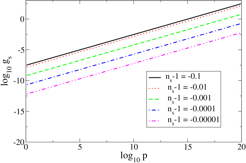
Figure 3: Log of the string coupling $g_{s}$ as a function of $\log_{10}p$ for several values of $n_{s}$.

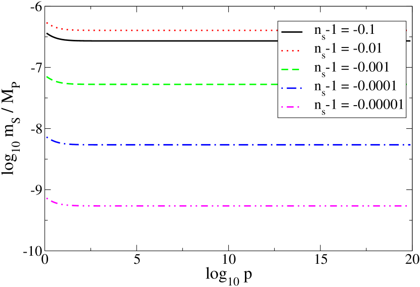
Figure 4: Log of the ratio of the string mass scale to the Planck mass as a function of $\log_{10}p$ for several values of $n_{s}$.

5.4 Comments on Slow Roll and the Relation to Local Field Theory

It is quite remarkable that our predictions for inflationary observables and also the solutions for $\chi$, $H$ are essentially identical to the results from local field theory with potential $V(\psi)=g_{s}(\psi^{2}-v^{2})^{2}/4$ where $g_{s}v^{2}\equiv 2m_{s}^{2}$ (see appendix C for a detailed comparison). Indeed, the dynamics of the $p$-adic tachyon are fixed by the mass scale in the kinetic term, $m_{s}$, rather than by the naive mass scale $\sqrt{-\partial^{2}V/\partial\chi^{2}}$ (see section 3), which may be much larger than $m_{s}$.

It is an interesting feature of this theory that the canonical $p$-adic tachyon, $\phi$, can roll slowly despite the fact that, working in a derivative truncatation (as in section 3), one would conclude that the tachyon has an extremely steep potential. To see this we first define the Hubble slow roll parameters $\epsilon_{\scriptscriptstyle H}$, $\eta_{\scriptscriptstyle H}$ by

$$\epsilon_{\scriptscriptstyle H} \equiv \frac{1}{2M_{p}^{2}}\frac{\dot{\varphi}^{2}}{H^{2}}$$ (81)

$$\epsilon_{\scriptscriptstyle H}-\eta_{\scriptscriptstyle H} \equiv \frac{\ddot{\varphi}}{H\dot{\varphi}}$$ (82)

These are the appropriate parameters to describe the rate of time variation of the inflaton as compared to the Hubble scale. Using the solution $\phi\cong 1-u$ (recall that $\varphi=A\phi$, $A=m_{s}p/(\sqrt{2}\,g_{s})$) we find that

$$\epsilon_{\scriptscriptstyle H} \cong \frac{1}{2}\frac{p+1}{p}e^{-60|n-1|}|n_{s}-1|$$ (83)

$$\eta_{\scriptscriptstyle H} \cong -\frac{|n_{s}-1|}{2}$$ (84)

We see that the Hubble slow-roll parameters, as defined above, are small. This means that the $p$-adic tachyon field rolls slowly in the conventional sense. One reaches the same conclusion if one defines the potential slow roll parameters using the correct canonical field, which is $\varphi$ (64):

$$\frac{M_{p}^{2}}{2}\left.\left(\frac{1}{V}\frac{\partial V}{\partial\varphi}\right)^{2}\right|_{\varphi=A} = 0$$ (85)

$$M_{p}^{2}\left.\frac{1}{V}\frac{\partial^{2}V}{\partial\varphi^{2}}\right|_{\varphi=A} = -\frac{1}{2}|n_{s}-1|$$ (86)

On the other hand, consider the potential slow roll parameter which one would naively define using the the derivative truncated action (4):

$$\frac{M_{p}^{2}}{2}\left.\left(\frac{1}{V}\frac{\partial V}{\partial\chi}\right)^{2}\right|_{\chi=\chi_{0}} = 0$$ (87)

$$M_{p}^{2}\left.\frac{1}{V}\frac{\partial^{2}V}{\partial\chi^{2}}\right|_{\chi=\chi_{0}} = -\left(\frac{p-1}{\ln p}\right)\,\frac{1}{2}|n_{s}-1|$$ (88)

where in (88) we have used equations (9) and (69). We see that (88) can be enormous, though the tachyon field rolls slowly. Taking the largest allowed value of $p$, $p\sim 10^{14}$, and $n_{s}\cong 0.95$ we have $M_{p}^{2}V^{-1}|\partial^{2}V/\partial\chi^{2}|\sim 10^{11}$!

Since large values of $p$ are required if one wants to obtain $g_{s}\sim 1$, it follows that it is somewhat natural for $p$-adic inflation to operate in the regime where the higher derivative corrections play an important role in the dyanimcs. However, in the regime where $p\sim 1$ (corresponding to very small coupling $g_{s}$) this novel features is not present. For example, with $p=3$, $n_{s}=0.95$ one has $g_{s}\sim 10^{-7}$ and $M_{p}^{2}V^{-1}|\partial^{2}V/\partial\chi^{2}|\sim 0.05$ and so the slow-roll dynamics are not surprising.

5.5 Tensor Modes

Since the $p$-adic stress tensor (4.2) does not contribute any anisotropic stresses up to first order in perturbation theory it follows that the first order tensor perturbations of the metric do not couple to the first order tachyon perturbation (see, for example, [31]). In fact, the action for the tensor perturbations is given by

$$S_{\mathrm{grav}}=\frac{M_{p}^{2}}{2}\int dt\,d^{\,3}x\,a(t)^{3}\,\frac{1}{2}\partial_{\mu}h_{ij}\,\partial^{\mu}h^{ij}$$

The standard procedure gives a power spectrum for the gravity waves

$$P_{T}=A_{T}^{2}\left(\frac{k}{aH_{0}}\right)^{n_{T}}$$

with amplitude

$$A_{T}^{2}=\frac{8}{M_{p}^{2}}\left(\frac{H_{0}}{2\pi}\right)^{2}$$ (89)

We would like to compare this to the power in scalar modes (77). Defining the tensor-to-scalar ratio in the usual way

$$r\equiv\frac{\frac{1}{100}A_{T}^{2}}{\frac{4}{25}A_{\zeta}^{2}}$$

we find that

$$r=\frac{1}{2M_{p}^{2}}\frac{\dot{\varphi}^{2}}{H_{0}^{2}}=\epsilon_{\scriptscriptstyle H}$$ (90)

which reproduces the usual result from local field theory. Using (83), we can evaluate $r$ as a function of $p$ and $n_{s}-1$

$$r=\frac{1}{2}\frac{p+1}{p}e^{-60|n_{s}-1|}|n_{s}-1|$$ (91)

It is easy to see that $r$ is maximal when $p=2$, $n_{s}=1-1/60$ and hence it follows that the scalar-tensor ratio is bounded from above as $r<0.006$, which is very small.

5.6 Comments on Initial Conditions

As we have previously noted, our classical solution $\phi(t)$ sits at the unstable maximum of the potential for an infinite amount of time, thus this model would seem to admit infinitely many e-foldings of inflation. Of course, this cannot be the case quantum mechanically and one expects quantum fluctuations to displace $\phi$ from the false vacuum and cause it to roll down the potential (we have assumed that this rolling takes place towards $\phi=0$, rather than down the unbounded side of the potential). As a consistency check we note that

$$\frac{\langle(\delta\phi)^{2}\rangle^{1/2}}{\phi_{0}}=\langle(\delta\phi)^{2}\rangle^{1/2}\sim\frac{H_{0}}{A}$$ (92)

We should compare this to $u_{\star}$ (see equation 75), the distance the field has rolled classically at horizon crossing. It is straightforward to show that

$$\frac{\langle(\delta\phi)^{2}\rangle^{1/2}}{u_{\star}}\sim 10^{-5}\,|n_{s}-1|$$

where we have used (78). Since $\langle(\delta\phi)^{2}\rangle^{1/2}\ll u_{\star}$ for all parameter values it follows that the de Sitter space fluctuations (which are present as $u\rightarrow 0$) will not displace the field far enough from the maximum of the potential to have any significant effect on the number of observable e-foldings of inflation, although they prevent inflation from being past-eternal. We note, however, that if one incorporates thermal fluctuations (and initial momentum) then this model may suffer from problems related to fine tuning the intial conditions as in small field inflationary models [33]. However, it is not clear if these objections apply to our model for several reasons. The first reason is that the dynamics of this theory is peculiar and it is not clear how (or if) the phase space arguments of [33] apply. The second reason is that it is not clear what initial conditions for the field $\phi$ are most natural from a string theory perspective. Finally we note that since the field $\varphi$ rolls a distance $A>M_{p}$ in field space, our model is not a “small field” model in the conventional sense.

If $p$-adic superstrings exist, it might also be possible to justify the initial conditions for inflation by having topological inflation [34], if the tachyon potential is symmetric about the unstable maximum. This distinction exists between the tachyon of the open bosonic string [8] (describing the instability of D25 branes), and the tachyon of unstable branes in superstring theory [35]. Any realistic extension of the model should have a potential which is bounded from below, and if it is supersymmetric, the minima should be at zero, hence the additional minima will be degenerate with the one at $\phi=0$. The existence of domains of the universe in the different minima ensures that there will be regions in between where inflation from the maximum of the potential is taking place, so long as the minima are discrete and not connected to each other by a continuous symmetry.

As we have noted previously the fact that the potential $V(\phi)$ is unbounded from below is thought to be a reflection of the closed string tachyonic instability of bosonic string theory. If this conjecture is correct then the addition of supersymmetry should indeed lead to a symmetric potential for the $p$-adic tachyon which is bounded from below, as we have suggested above.

6 Conclusions

In this paper we have constructed for the first time approximate solutions of the fully nonlocal $p$-adic string theory coupled to gravity, in which the $p$-adic tachyon drives a sufficiently long period of inflation while rolling away from the maximum of its potential. In our solution, the nonlocal nature of the theory played an essential role in obtaining slow-roll, since with a conventional kinetic term the potential would have been too steep to give inflation. One of the novel features of this construction is that the Hubble parameter is larger than the string scale during inflation, a condition which would usually invalidate an effective field theory description, but which is consistent in the present context because of the ultraviolet-complete nature of the theory.

We found that the experimental constraints on the amplitude of the spectrum of scalar perturbations produced by inflation require a small value of the string coupling $g_{s}$, and can be consistent with a large range of values of the parameter $p$, $1\mbox{\raisebox{-2.58334pt}{~{}$\stackrel{{\scriptstyle<}}{{\sim}}$~{}}}p\mbox{\raisebox{-2.58334pt}{~{}$\stackrel{{\scriptstyle<}}{{\sim}}$~{}}}10^{14}$. The regime $p\gg 1$ is interesting because it exhibits qualitatively different behavior relative to conventional inflationary models: slow roll despite the potential being steep, and inflation being driven by the kinetic as well as potential energy of the field. This regime is also interesting because it corresponds to $g_{s}=\mathcal{O}(1)$ and hence appears more natural from a string theory perspective. Since the $p$-adic string is not construed to be a realistic model by itself, it may not be very meaningful to question how natural such values might be. However, it may not be unreasonable to think of real strings as being composed of constituent $p$-adic strings because the Veneziano amplitude of the $p$-adic theory is related to that of the full bosonic string by ${\cal A}^{-1}=\prod_{p}{\cal A}_{p}$ where the product is over all prime numbers $p$. Thus it may not be unreasonable to expect similar behavior to the large-$p$ results from a more realistic model.

The model predicts a red spectrum, in agreement with the latest WMAP data, whose tilt is related to the ratio of the string scale to the Hubble rate during inflation via $H/m_{s}=2/\sqrt{3|n_{s}-1|}$. For $n_{s}=0.95$ this gives $H/m_{s}\cong 5$. This is in contrast to most stringy models of inflation which require $H<m_{s}$ in order for the effective field theory to be valid. We find the bound $r<0.006$ on the tensor modes. It has been estimated that future experiments could eventually have a sensitivity of $r\sim 6\times 10^{-5}$ [36] and hence the tensor components may in fact be observable.

We noted that the $p$-adic model succeeds with inflation where the real string theory tachyon fails. But our analysis makes it clear that this could be due to the failure to keep terms with arbitrary numbers of derivatives in the action. The effective tachyon action of Sen [17] is a truncation which keeps arbitrary powers of first derivatives but ignores higher order derivatives, which were essential for obtaining our solution. Thus the new features for inflation which we find in $p$-adic string theory could also be present in realistic string theories, if we knew how to include the whole tower of higher dimensional kinetic terms.

Note Added

Upon completing this paper a related work appeared [38] in which an alternative normalization for the fluctuations of the $p$-adic scalar was proposed. Motivated by this work, we reconsidered our choice of normalization and concluded that (64,65) is the most appropriate definition of a “canonical” field. Notice, however, that our field $\varphi$ differs from the definition of a canonical field which was proposed in [38]. In [38] a field redefinition is advocated which puts the stress tensor $T_{\mu\nu}$ into canonical form, though this definition does not have canonical kinetic term in the action. Though we believe that our definition is more natural, we stress that in the case of current interest, $p$-adic inflation, the distinction does not generate any significant quantitative difference because our definition differs from that of [38] by a factor proportional to $\sqrt{\ln p}$ (which is less than an order of magnitude for the values of $p$ which we consider). We are grateful to J. Lidsey for sending us a draft of his manuscript prior to publication and also for interesting and enlightening discussions.

Appendix A The Stress Energy Tensor and the Friedmann Equation

Here we compute the $O(u^{2})$ term of the approximate solutions

$$\phi = 1-u-\phi_{2}u^{2}$$

$$H = H_{0}-H_{2}u^{2}$$

We write the different terms appearing in the energy density as

$$\rho_{\phi}=-T_{00}={m_{s}^{4}\over 2g_{p}^{2}}\left[\phi e^{-{\Box\over m_{p}^{2}}}\phi-{2\over p+1}\phi^{p+1}+{1\over m_{p}^{2}}\int_{0}^{1}d\tau\ \left(\Box e^{-{\tau\Box\over m_{p}^{2}}}\phi\right)\left(e^{-{(1-\tau)\Box\over m_{p}^{2}}}\phi\right)\right.$$

$$\left.+{1\over m_{p}^{2}}\int_{0}^{1}d\tau\ \partial_{t}\left(e^{-{\tau\Box\over m_{p}^{2}}}\phi\right)\partial_{t}\left(e^{-{(1-\tau)\Box\over m_{p}^{2}}}\phi\right)\right]\equiv{m_{s}^{4}\over 2g_{p}^{2}}(T_{1}+T_{2}+T_{3}+T_{4})$$ (A-1)

where $T_{1}$, $T_{2}$, $T_{3}$ and $T_{4}$ are defined as in (49-52). We now evaluate this expression term-by-term.

We first consider $T_{1}+T_{2}$, which can be written as

$$T_{1}+T_{2}=\frac{p-1}{p+1}\phi^{p+1}$$

using (3). Using (A) we have

$$T_{1}+T_{2}=\frac{p-1}{p+1}+(-p+1)u+(p-1)\left[-\phi_{2}+\frac{p}{2}\right]u^{2}+\mathcal{O}(u^{3})$$ (A-2)

To evaluate $T_{3}$, $T_{4}$ we note that

$$e^{-\tau\Box/m_{p}^{2}}\phi = 1-e^{\tau\mu_{1}}u-\phi_{2}e^{\tau\mu_{2}}u^{2}+\cdots$$

$$e^{-(1-\tau)\Box/m_{p}^{2}}\phi = 1-e^{(1-\tau)\mu_{1}}u-\phi_{2}e^{(1-\tau)\tau\mu_{2}}u^{2}+\cdots$$ (A-3)

(see equation 23 with $\sigma=0$). It is straightforward to show that

$$\Box e^{-\tau\Box/m_{p}^{2}}\phi=e^{\tau\mu_{1}}(\lambda^{2}+3H_{0}\lambda)u+\phi_{2}e^{\tau\mu_{2}}(4\lambda^{2}+3H_{0}\lambda)u^{2}+\cdots$$ (A-4)

We are now in a position to compute $T_{3}$. Using (A-3) and (A-4) we have

$$T_{3} = \frac{1}{m_{p}^{2}}\int_{0}^{1}d\tau\left[(\lambda^{2}+3H_{0}\lambda)e^{\tau\mu_{1}}u\right.$$

$$+ \left.\left[-(\lambda^{2}+3H_{0}\lambda)e^{\mu_{1}}+\phi_{2}(4\lambda^{2}+6H_{0}\lambda)e^{\tau\mu_{2}}\right]u^{2}+\cdots\right]$$

The $d\tau$ integrals are trivial to perform using the identity

$$\int_{0}^{1}d\tau e^{\alpha\tau}=\frac{e^{\alpha}-1}{\alpha}$$ (A-5)

We find that

$$T_{3}=(p-1)u+\left[-p\mu_{1}+(e^{\mu_{2}}-1)\phi_{2}\right]u^{2}+\mathcal{O}(u^{3})$$ (A-6)

We now consider the integrand of $T_{4}$:

$$\partial_{t}\left(e^{-{\tau\Box\over m_{p}^{2}}}\phi\right)\partial_{t}\left(e^{-{(1-\tau)\Box\over m_{p}^{2}}}\phi\right)\cong\lambda^{2}u^{2}\partial_{u}\left(1-e^{\tau\mu_{1}}u\right)\partial_{u}\left(1-e^{(1-\tau)\mu_{1}}u\right)=\lambda^{2}u^{2}e^{\mu_{1}}$$ (A-7)

The $d\tau$ integral is trivial and gives

$$T_{4}=u^{2}{\lambda^{2}\over m_{p}^{2}}e^{\mu_{1}}$$ (A-8)

It is straightforward to sum up the various contributions to $T_{00}$. We find that

$$\rho_{\phi} = \frac{m_{s}^{4}}{2g_{p}^{2}}\left[\frac{p-1}{p+1}\right.$$ (A-9)

$$+ \left.\left[(-p+e^{\mu_{2}})\phi_{2}+\frac{p}{2}(p-1)-p\ln p+p\frac{\lambda^{2}}{m_{p}^{2}}\right]u^{2}+\cdots\right]$$

The fact that the coefficient of the $\mathcal{O}(u)$ term is zero verifies that $H_{1}=0$. We now solve the Friedmann equation

$$3H^{2}=\frac{1}{M_{p}^{2}}\rho_{\phi}$$

noting that

$$H^{2}=H_{0}^{2}-2H_{0}H_{2}u^{2}+\mathcal{O}(u^{3})$$

Matching the coefficients at order $u^{0}$ gives

$$H_{0}^{2}=\frac{1}{6g_{p}^{2}}\frac{m_{s}^{4}}{M_{p}^{2}}\frac{p-1}{p+1}$$

as before. Matching the coefficients at order $u^{2}$ gives

$$-6H_{0}H_{2} = \frac{m_{s}^{4}}{2g_{p}^{2}M_{p}^{2}}\left[(e^{\mu_{2}}-p)\phi_{2}+\frac{p}{2}(p-1)-p\ln p+p\frac{\lambda^{2}}{m_{p}^{2}}\right]$$

$$= \frac{m_{s}^{4}}{M_{p}^{2}}\frac{p}{2g_{p}^{2}}\left[\frac{\lambda^{2}}{m_{p}^{2}}-\ln p\right]$$

$$= \frac{m_{s}^{4}}{M_{p}^{2}}\frac{p}{2g_{p}^{2}}\left[\frac{-3H_{0}\lambda}{m_{p}^{2}}\right]$$

In the first equality we have used that fact that

$$\phi_{2}e^{\mu_{2}}=p\phi_{2}-\frac{p}{2}(p-1)$$

which follows from the second order Klein-Gordon equation and in the second equality we have used

$$\frac{\lambda^{2}}{m_{p}^{2}}+3\frac{H_{0}\lambda}{m_{p}^{2}}=\mu_{1}=\ln p$$

which follows from the first order Klein-Gordon equation. Finally we arive at the result for $H_{2}$:

$$H_{2}=\frac{m_{s}^{4}}{4g_{p}^{2}M_{p}^{2}}\frac{p\lambda}{m_{p}^{2}}=\frac{1}{8g_{s}^{2}}\frac{p^{3}\ln p}{p-1}\left(\frac{m_{s}}{M_{p}}\right)^{2}\lambda$$ (A-10)

Appendix B Incomplete Cylindrical Functions of the Sonine-Schaefli Form

The Bessel function can be represented by a contour integral of the Sonine-Schaefli form

$$J_{\nu}(z)=\frac{1}{2\pi i}\left(\frac{z}{2}\right)^{\nu}\int_{c-i\infty}^{c+i\infty}\omega^{-\nu-1}\exp\left[\omega-\frac{z^{2}}{4\omega}\right]d\omega$$ (B-1)

as long as $\mathrm{Re}(\nu)>-1$. In (B-1) $c$ is an arbitrary positive constant. The incomplete cylindrical function, $S_{\nu}(r,s;z)$ generalizes (B-1) to arbitrary limits of integration

$$S_{\nu}(r,s;z)=\frac{1}{2\pi i}\left(\frac{z}{2}\right)^{\nu}\int_{r}^{s}\omega^{-\nu-1}\exp\left[\omega-\frac{z^{2}}{4\omega}\right]d\omega$$ (B-2)

It follows that

$$\int_{r}^{s}\omega^{-\nu-1}\exp\left[-\omega-\frac{z^{2}}{4\omega}\right]d\omega=2\pi ie^{i\nu\pi/2}\left(\frac{z}{2}\right)^{-\nu}S(-r,-s;iz)$$ (B-3)

Taking the limits $r\rightarrow 0$ and $s\rightarrow+\infty$ this integral can be written in terms of Hankel functions of imaginary argument, $K_{\nu}(z)$, as

$$\int_{0}^{\infty}\omega^{-\nu-1}\exp\left[-\omega-\frac{z^{2}}{4\omega}\right]d\omega=2\left(\frac{z}{2}\right)^{-\nu}K_{\nu}(z)$$ (B-4)

The function $K_{\nu}(z)$ is real-valued for real $z$ and is related to the usual Hankel function as $K_{\nu}(z)=(i\pi/2)e^{i\pi\nu/2}H_{\nu}^{(1)}(iz)$. Using the well known large-argument asymptotics of the Hankel functions one may show that

$$\int_{0}^{\infty}\omega^{-\nu-1}\exp\left[-\omega-\frac{z^{2}}{4\omega}\right]d\omega\cong\sqrt{\frac{2\pi}{z}}\left(\frac{z}{2}\right)^{-\nu}e^{-z}$$ (B-5)

for $z\gg 1$.

Appendix C Comparison to Local Field Theory

In this appendix we perform a detailed comparison of our results for the action (1) to the theory

$$S=-\int d^{4}x\left[\frac{1}{2}\partial_{\mu}\psi\partial^{\mu}\psi+V(\psi)\right]$$ (C-1)

with potential

$$V(\psi) = \frac{g_{s}}{4}\left(\psi^{2}-v^{2}\right)^{2}$$ (C-2)

$$\equiv \frac{gv^{4}}{4}-m_{s}^{2}\psi^{2}+\frac{g}{4}\psi^{4}$$

where we have defined $m_{s}^{2}\equiv 2g_{s}v^{2}$. We are interested in obtaining inflation near the unstable maximum $\psi=0$. The flatness of the potential is parameterized by the dimensionless slow roll parameters

$$\epsilon = \frac{M_{p}^{2}}{2}\left(\frac{V^{\prime\prime}(\psi)}{V(\psi)}\right)^{2}=\frac{8\psi^{2}M_{p}^{2}}{(\psi^{2}-v^{2})^{2}}$$ (C-3)

$$\eta = M_{p}^{2}\frac{V^{\prime\prime}(\psi)}{V(\psi)}=\frac{4M_{p}^{2}}{(\psi^{2}-v^{2})^{2}}\left[3\psi^{2}-v^{2}\right]$$ (C-4)

Unlike in the $p$-adic theory we do not need to distinguish between $\epsilon_{\scriptscriptstyle H},\eta_{\scriptscriptstyle H}$ and $\epsilon_{V},\eta_{V}$ (see equations 81-88) and hence we drop the subscripts on the slow roll parameters. For $\psi\ll v$ the $\epsilon$ parameter (C-3) is automatically small while

$$|\eta|\cong 8\left(\frac{M_{p}}{v}\right)^{2}$$

which is small compared to unity for $v\gg M_{p}$. The fact that the symmetry breaking scale is large compared to the Planck scale may be reason to doubt the validity of the field theory (C-1). However, for our purposes this is irrelevant.

It is instructive to consider solving the equations of motion for this theory using the formalism of section 4. We begin by speculating solutions of the form

$$\psi = ve^{\lambda t}+\psi_{2}ve^{2\lambda t}+\psi_{3}ve^{3\lambda t}+\mathcal{O}(e^{3\lambda t})$$ (C-5)

$$H = H_{0}-H_{1}e^{\lambda t}-H_{2}e^{2\lambda t}+\mathcal{O}(e^{3\lambda t})$$ (C-6)

and solving order by order in $e^{\lambda t}$. The ansatz (C-5,C-6) is analogous to (11,12) since in both cases the (classical) field spends an infinite amount of time at the unstable maximum, driving a past-eternal de Sitter phase, before rolling towards the true minimum of the potential. We suppose that $e^{\lambda t}\ll 1$ so that $\psi\ll v$ initially.

The Klein-Gordon equation is

$$\frac{\ddot{\psi}}{v}+3H\frac{\dot{\psi}}{v}=2m_{s}^{2}\frac{\psi}{v}+2m_{s}^{2}\left(\frac{\psi}{v}\right)^{3}$$

Plugging in the ansatz (C-5) we obtain

$$\lambda^{2}+3H_{0}\lambda=2m_{s}^{2}$$ (C-7)

at first order in $e^{\lambda t}$. This result is identical to (27). At second and third order respectively we find

$$\psi_{2} = 0$$

$$\psi_{3} = \frac{2m_{s}^{2}+3H_{2}\lambda}{9\lambda^{2}-2m_{s}^{2}}$$

The Friedmann equation is

$$3H^{2}=\frac{1}{M_{p}^{2}}\left[\frac{gv^{4}}{4}-m_{s}^{2}v^{2}\left(\frac{\psi}{v}\right)^{2}+\frac{gv^{4}}{4}\left(\frac{\psi}{v}\right)^{4}+\frac{v^{2}}{2}\left(\frac{\dot{\psi}}{v}\right)^{2}\right]$$

At zeroth order in $e^{\lambda t}$ we obtain the familiar result

$$H_{0}=\frac{g^{1/2}}{2\sqrt{3}}\frac{v^{2}}{M_{p}}$$ (C-8)

At first and second order we find that

$$H_{1} = 0$$ (C-9)

$$H_{2} = \frac{2}{\sqrt{3g}}\frac{2m_{s}^{2}-\lambda^{2}}{M_{p}}=\frac{1}{4}\left(\frac{v}{M_{p}}\right)^{2}\lambda$$ (C-10)

In writing the second equality in (C-10) we have used $\lambda^{2}+3H_{0}\lambda=2m_{s}^{2}$.

Though a complete treatment of inhomogeneities including metric perturbations and nonzero slow roll parameters is straightforward in this context we choose to analyze this theory using the same approximations as we used in section 5 in order to make more explicit the comparison between the two theories. The perturbed Klein-Gordon equation (neglecting metric fluctuations and in the limit $e^{\lambda t}\rightarrow 0$) is

$$\left(\partial_{t}^{2}+3H_{0}\partial_{t}-\frac{\partial_{i}\partial^{i}}{a^{2}}-2m_{s}^{2}\right)\delta\psi=0$$

where $a=e^{H_{0}t}$. The large scale solution is

$$|\delta\psi_{k}|\cong\frac{H}{\sqrt{2k^{3}}}\left(\frac{k}{aH_{0}}\right)^{3/2-\nu}$$

where

$$\nu=\sqrt{\frac{9}{4}+\frac{2m_{s}^{2}}{H_{0}^{2}}}$$

Near scale-invariance of the spectrum requires $m_{s}\ll H_{0}$. In this limit we have

$$n_{s}-1\cong-\frac{4}{3}\frac{m_{s}^{2}}{H_{0}^{2}}=-8\left(\frac{M_{p}}{v}\right)^{2}$$ (C-11)

which is identical to (68). This result also reproduces the full calculation incorporating metric perturbations: $n_{s}-1\cong 2\eta-6\epsilon\cong-8M_{p}^{2}/v^{2}$.

We can use (C-11) to write the dimensionless quantities $H_{0}/m_{s}$, $H_{2}/m_{s}$ and $\lambda/m_{s}$ in terms of $|n_{s}-1|$. The solution of (C-7) can be written as

$$\frac{\lambda}{m_{s}}\cong\sqrt{\frac{|n_{s}-1|}{3}}$$

which is identical to (71). For this solution we of course have $3\lambda H_{0}\gg\lambda^{2}$ so that the evolution is friction dominated. It is also straightforward to show that

$$\frac{H_{0}}{m_{s}} = \frac{2}{\sqrt{3|n_{s}-1|}}$$

$$H_{2} = H_{0}$$

We see that the solutions $H$, $\chi$ for the theory (C-1) are identical to those of the theory (1) up to order $e^{\lambda t}$. At order $e^{2\lambda t}$ and higher, however, the dynamics of the two theories differs.

From (C-3) one can check that $\epsilon\cong 1$ at $\psi\mbox{\raisebox{-2.58334pt}{~{}$\stackrel{{\scriptstyle<}}{{\sim}}$~{}}}v$ so that it is a good approximation to suppose that inflation ends at $e^{\lambda t}\cong 1$. It is straightforward to impose the COBE normalization $V/(\epsilon M_{p}^{4})=6\times 10^{-7}$ for this model (which will impose $g_{s}\ll|n_{s}-1|^{2}$), however, this is unnecessary for our purposes. It is clear that the inflationary dynamics and predictions predictions of the theory (C-1) are identical to those of the theory (1).

References

- [1] G. R. Dvali and S. H. H. Tye, “Brane inflation,” Phys. Lett. B 450, 72 (1999) [arXiv:hep-ph/9812483]. C. P. Burgess, M. Majumdar, D. Nolte, F. Quevedo, G. Rajesh and R. J. Zhang, “The inflationary brane-antibrane universe,” JHEP 0107, 047 (2001) [arXiv:hep-th/0105204]. J. Garcia-Bellido, R. Rabadan and F. Zamora, “Inflationary scenarios from branes at angles,” JHEP 0201, 036 (2002) [arXiv:hep-th/0112147]. N. T. Jones, H. Stoica and S. H. H. Tye, “Brane interaction as the origin of inflation,” JHEP 0207, 051 (2002) [arXiv:hep-th/0203163]. D. Choudhury, D. Ghoshal, D. P. Jatkar and S. Panda, “Hybrid inflation and brane-antibrane system,” JCAP 0307, 009 (2003) [arXiv:hep-th/0305104]. S. Kachru, R. Kallosh, A. Linde, J. M. Maldacena, L. McAllister and S. P. Trivedi, “Towards inflation in string theory,” JCAP 0310, 013 (2003) [arXiv:hep-th/0308055]. C. P. Burgess, J. M. Cline, H. Stoica and F. Quevedo, “Inflation in realistic D-brane models,” JHEP 0409, 033 (2004) [arXiv:hep-th/0403119]. J. M. Cline and H. Stoica, “Multibrane inflation and dynamical flattening of the inflaton potential,” Phys. Rev. D 72, 126004 (2005) [arXiv:hep-th/0508029]. D. Baumann, A. Dymarsky, I. R. Klebanov, J. Maldacena, L. McAllister and A. Murugan, “On D3-brane potentials in compactifications with fluxes and wrapped D-branes,” JHEP 0611, 031 (2006) [arXiv:hep-th/0607050]. C. P. Burgess, J. M. Cline, K. Dasgupta and H. Firouzjahi, “Uplifting and inflation with D3 branes,” arXiv:hep-th/0610320.
- [2] K. Dasgupta, C. Herdeiro, S. Hirano and R. Kallosh, “D3/D7 inflationary model and M-theory,” Phys. Rev. D 65, 126002 (2002) [arXiv:hep-th/0203019]. K. Dasgupta, J. P. Hsu, R. Kallosh, A. Linde and M. Zagermann, “D3/D7 brane inflation and semilocal strings,” JHEP 0408, 030 (2004) [arXiv:hep-th/0405247]. P. Chen, K. Dasgupta, K. Narayan, M. Shmakova and M. Zagermann, “Brane inflation, solitons and cosmological solutions: I,” JHEP 0509, 009 (2005) [arXiv:hep-th/0501185].
- [3] J. J. Blanco-Pillado et al., “Racetrack inflation,” JHEP 0411, 063 (2004) [arXiv:hep-th/0406230]. J. P. Conlon and F. Quevedo, “Kaehler moduli inflation,” JHEP 0601, 146 (2006) [arXiv:hep-th/0509012]. J. J. Blanco-Pillado et al., “Inflating in a better racetrack,” JHEP 0609, 002 (2006) [arXiv:hep-th/0603129]. J. R. Bond, L. Kofman, S. Prokushkin and P. M. Vaudrevange, “Roulette Inflation with Kahler Moduli and their Axions,” arXiv:hep-th/0612197.
- [4] E. Silverstein and D. Tong, “Scalar speed limits and cosmology: Acceleration from D-cceleration,” Phys. Rev. D 70, 103505 (2004) [arXiv:hep-th/0310221]. M. Alishahiha, E. Silverstein and D. Tong, “DBI in the sky,” Phys. Rev. D 70, 123505 (2004) [arXiv:hep-th/0404084]. X. Chen, “Multi-throat brane inflation,” Phys. Rev. D 71, 063506 (2005) [arXiv:hep-th/0408084]. X. Chen, “Inflation from warped space,” JHEP 0508, 045 (2005) [arXiv:hep-th/0501184]. S. E. Shandera and S. H. Tye, “Observing brane inflation,” JCAP 0605, 007 (2006) [arXiv:hep-th/0601099]. S. Kecskemeti, J. Maiden, G. Shiu and B. Underwood, “DBI inflation in the tip region of a warped throat,” JHEP 0609, 076 (2006) [arXiv:hep-th/0605189]. S. H. Tye, “Brane inflation: String theory viewed from the cosmos,” arXiv:hep-th/0610221.
- [5] M. Fairbairn and M. H. G. Tytgat, “Inflation from a tachyon fluid?,” Phys. Lett. B 546, 1 (2002) [arXiv:hep-th/0204070]. D. Choudhury, D. Ghoshal, D. P. Jatkar and S. Panda, “On the cosmological relevance of the tachyon,” Phys. Lett. B 544, 231 (2002) [arXiv:hep-th/0204204]. A. Feinstein, “Power-law inflation from the rolling tachyon,” Phys. Rev. D 66, 063511 (2002) [arXiv:hep-th/0204140]. M. Sami, “Implementing power law inflation with rolling tachyon on the brane,” Mod. Phys. Lett. A 18, 691 (2003) [arXiv:hep-th/0205146]. Y. S. Piao, R. G. Cai, X. m. Zhang and Y. Z. Zhang, “Assisted tachyonic inflation,” Phys. Rev. D 66, 121301 (2002) [arXiv:hep-ph/0207143]. M. Majumdar and A. C. Davis, “Inflation from tachyon condensation, large N effects,” Phys. Rev. D 69, 103504 (2004) [arXiv:hep-th/0304226]. D. A. Steer and F. Vernizzi, “Tachyon inflation: Tests and comparison with single scalar field inflation,” Phys. Rev. D 70, 043527 (2004) [arXiv:hep-th/0310139]. J. Raeymaekers, “Tachyonic inflation in a warped string background,” JHEP 0410, 057 (2004) [arXiv:hep-th/0406195]. D. Cremades, F. Quevedo and A. Sinha, “Warped tachyonic inflation in type IIB flux compactifications and the open-string completeness conjecture,” JHEP 0510, 106 (2005) [arXiv:hep-th/0505252]. D. Cremades, “Electric tachyon inflation,” Fortsch. Phys. 54, 357 (2006) [arXiv:hep-th/0512294]. L. Leblond and S. Shandera, “Cosmology of the tachyon in brane inflation,” arXiv:hep-th/0610321.
- [6] J. M. Cline, “String cosmology,” arXiv:hep-th/0612129.
- [7] P. G. O. Freund and M. Olson, “Nonarchimedean strings,” Phys. Lett. B 199, 186 (1987); P. G. O. Freund and E. Witten, “Adelic string amplitudes,” Phys. Lett. B 199, 191 (1987). L. Brekke, P.G. Freud, M. Olson and E. Witten, “Nonarchimedean String Dynamics,” Nucl. Phys. B 302, 365 (1998).
- [8] D. Kutasov, M. Marino and G. W. Moore, “Some exact results on tachyon condensation in string field theory,” JHEP 0010, 045 (2000) [arXiv:hep-th/0009148].
- [9] L. Kofman and A. Linde, “Problems with tachyon inflation,” JHEP 0207, 004 (2002) [arXiv:hep-th/0205121].
- [10] R. P. Woodard, “Avoiding dark energy with 1/R modifications of gravity,” arXiv:astro-ph/0601672.
- [11] N. Moeller and B. Zwiebach, “Dynamics with infinitely many time derivatives and rolling tachyons,” JHEP 0210, 034 (2002) [arXiv:hep-th/0207107].
- [12] T. Biswas, A. Mazumdar and W. Siegel, “Bouncing universes in string-inspired gravity,” JCAP 0603, 009 (2006) [arXiv:hep-th/0508194]; T. Biswas, R. Brandenberger, A. Mazumdar and W. Siegel, “Non-perturbative gravity, Hagedorn bounce and CMB,” arXiv:hep-th/0610274.
- [13] J. Khoury, “Fading Gravity and Self-Inflation,” arXiv:hep-th/0612052.
- [14] A. A. Gerasimov and S. L. Shatashvili, “On exact tachyon potential in open string field theory,” JHEP 0010, 034 (2000) [arXiv:hep-th/0009103].
- [15] D. Ghoshal and A. Sen, “Tachyon condensation and brane descent relations in -adic string theory,” Nucl. Phys. B 584, 300 (2000) [arXiv:hep-th/0003278].
- [16] P. H. Frampton and H. Nishino, “STABILITY ANALYSIS OF P-ADIC STRING SOLITONS,” Phys. Lett. B 242, 354 (1990). J. A. Minahan, “Mode interactions of the tachyon condensate in -adic string theory,” JHEP 0103, 028 (2001) [arXiv:hep-th/0102071]. N. Moeller and M. Schnabl, “Tachyon condensation in open-closed -adic string theory,” JHEP 0401, 011 (2004) [arXiv:hep-th/0304213].
- [17] M. R. Garousi, “Tachyon couplings on nonBPS D-branes and Dirac-Born-Infeld action,” Nucl. Phys. B 584, 284 (2000) [arXiv:hep-th/0003122]. E. A. Bergshoeff, M. de Roo, T. C. de Wit, E. Eyras and S. Panda, “T-duality and actions for nonBPS D-branes,” JHEP 0005, 009 (2000) [arXiv:hep-th/0003221]. J. Kluson, “Proposal for non-BPS D-brane action,” Phys. Rev. D 62, 126003 (2000) [arXiv:hep-th/0004106]. A. Sen, “Tachyon matter,” JHEP 0207, 065 (2002) [arXiv:hep-th/0203265]. A. Sen, “Field theory of tachyon matter,” Mod. Phys. Lett. A 17, 1797 (2002) [arXiv:hep-th/0204143]. A. Sen, “Dirac-Born-Infeld action on the tachyon kink and vortex,” Phys. Rev. D 68, 066008 (2003) [arXiv:hep-th/0303057].
- [18] D. Ghoshal, “p-adic string theories provide lattice discretization to the ordinary string worldsheet,” Phys. Rev. Lett. 97, 151601 (2006).
- [19] G. W. Gibbons, K. Hori and P. Yi, “String fluid from unstable D-branes,” Nucl. Phys. B 596, 136 (2001) [arXiv:hep-th/0009061]. A. Sen, “Rolling tachyon,” JHEP 0204, 048 (2002) [arXiv:hep-th/0203211]. G. N. Felder, L. Kofman and A. Starobinsky, “Caustics in tachyon matter and other Born-Infeld scalars,” JHEP 0209, 026 (2002) [arXiv:hep-th/0208019]. G. Gibbons, K. Hashimoto and P. Yi, “Tachyon condensates, Carrollian contraction of Lorentz group, and fundamental strings,” JHEP 0209, 061 (2002) [arXiv:hep-th/0209034]. F. Larsen, A. Naqvi and S. Terashima, “Rolling tachyons and decaying branes,” JHEP 0302, 039 (2003) [arXiv:hep-th/0212248]. O. K. Kwon and P. Yi, “String fluid, tachyon matter, and domain walls,” JHEP 0309, 003 (2003) [arXiv:hep-th/0305229]. G. N. Felder and L. Kofman, “Inhomogeneous fragmentation of the rolling tachyon,” Phys. Rev. D 70, 046004 (2004) [arXiv:hep-th/0403073].
- [20] E. Coletti, I. Sigalov and W. Taylor, “Taming the tachyon in cubic string field theory,” JHEP 0508, 104 (2005) [arXiv:hep-th/0505031].
- [21] I. Y. Aref’eva, L. V. Joukovskaya and A. S. Koshelev, “Time evolution in superstring field theory on non-BPS brane. I: Rolling tachyon and energy-momentum conservation,” JHEP 0309, 012 (2003) [arXiv:hep-th/0301137]. M. Fujita and H. Hata, “Rolling tachyon solution in vacuum string field theory,” Phys. Rev. D 70, 086010 (2004) [arXiv:hep-th/0403031]. T. G. Erler, “Level truncation and rolling the tachyon in the lightcone basis for open string field theory,” arXiv:hep-th/0409179. V. Forini, G. Grignani and G. Nardelli, “A new rolling tachyon solution of cubic string field theory,” arXiv:hep-th/0502151. V. Forini, G. Grignani and G. Nardelli, “A solution to the 4-tachyon off-shell amplitude in cubic string field theory,” JHEP 0604, 053 (2006) [arXiv:hep-th/0603206].
- [22] M. R. Douglas and S. H. Shenker, “Strings In Less Than One-Dimension,” Nucl. Phys. B 335, 635 (1990); D. J. Gross and A. A. Migdal, “Nonperturbative Two-Dimensional Quantum Gravity,” Phys. Rev. Lett. 64, 127 (1990); E. Brezin and V. A. Kazakov, “EXACTLY SOLVABLE FIELD THEORIES OF CLOSED STRINGS,” Phys. Lett. B 236, 144 (1990).
- [23] T. Biswas, M. Grisaru and W. Siegel, “Linear Regge trajectories from worldsheet lattice parton field theory,” Nucl. Phys. B 708, 317 (2005) [arXiv:hep-th/0409089].
- [24] I. Y. Aref’eva, “Nonlocal string tachyon as a model for cosmological dark energy,” AIP Conf. Proc. 826, 301 (2006) [arXiv:astro-ph/0410443]. I. Y. Aref’eva and L. V. Joukovskaya, “Time lumps in nonlocal stringy models and cosmological applications,” JHEP 0510, 087 (2005) [arXiv:hep-th/0504200]. I. Y. Aref’eva, A. S. Koshelev and S. Y. Vernov, “Crossing of the w = -1 barrier by D3-brane dark energy model,” Phys. Rev. D 72, 064017 (2005) [arXiv:astro-ph/0507067]. G. Calcagni, “Cosmological tachyon from cubic string field theory,” JHEP 0605, 012 (2006) [arXiv:hep-th/0512259]. I. Y. Aref’eva and A. S. Koshelev, “Cosmic acceleration and crossing of w = -1 barrier from cubic superstring field theory,” arXiv:hep-th/0605085. I. Y. Aref’eva and I. V. Volovich, “On the null energy condition and cosmology,” arXiv:hep-th/0612098.
- [25] M. Laidlaw and M. Nishimura, “Comments on higher derivative terms for the tachyon action,” arXiv:hep-th/0403269.
- [26] H. t. Yang, “Stress tensors in -adic string theory and truncated OSFT,” JHEP 0211, 007 (2002) [arXiv:hep-th/0209197].
- [27] A. Sen, “Energy momentum tensor and marginal deformations in open string field theory,” JHEP 0408, 034 (2004) [arXiv:hep-th/0403200].
- [28] N. Barnaby, “Caustic formation in tachyon effective field theories,” JHEP 0407, 025 (2004) [arXiv:hep-th/0406120].
- [29] D. N. Spergel et al., “Wilkinson Microwave Anisotropy Probe (WMAP) three year results: Implications for cosmology,” arXiv:astro-ph/0603449.
- [30] Y. Volovich, “Numerical study of nonlinear equations with infinite number of derivatives,” J. Phys. A 36, 8685 (2003) [arXiv:math-ph/0301028]. V. S. Vladimirov and Y. I. Volovich, “On the nonlinear dynamical equation in the -adic string theory,” Theor. Math. Phys. 138, 297 (2004) [Teor. Mat. Fiz. 138, 355 (2004)] [arXiv:math-ph/0306018]. V. S. Vladimirov, “On the equation of the -adic open string for the scalar tachyon field,” arXiv:math-ph/0507018. D. V. Prokhorenko, “On Some Nonlinear Integral Equation in the (Super)String Theory,” arXiv:math-ph/0611068.
- [31] V. F. Mukhanov, H. A. Feldman and R. H. Brandenberger, “Theory of cosmological perturbations. Part 1. Classical perturbations. Part 2. Quantum theory of perturbations. Part 3. Extensions,” Phys. Rept. 215, 203 (1992). A. Riotto, “Inflation and the theory of cosmological perturbations,” arXiv:hep-ph/0210162. D. Langlois, “Inflation, quantum fluctuations and cosmological perturbations,” arXiv:hep-th/0405053.
- [32] M. M. Agrest, M. S. Maksimov, “Theory on Incomplete Cylindrical Functions and their Applications,” Springer-Verlag Berlin Heidelberg New York, 1971.
- [33] D. S. Goldwirth, “Initial Conditions For New Inflation,” Phys. Lett. B 243, 41 (1990). D. S. Goldwirth and T. Piran, “Initial conditions for inflation,” Phys. Rept. 214, 223 (1992). R. Brandenberger, G. Geshnizjani and S. Watson, “On the initial conditions for brane inflation,” Phys. Rev. D 67, 123510 (2003) [arXiv:hep-th/0302222].
- [34] A. D. Linde, “Monopoles as big as a universe,” Phys. Lett. B 327, 208 (1994) [arXiv:astro-ph/9402031]; A. D. Linde and D. A. Linde, “Topological defects as seeds for eternal inflation,” Phys. Rev. D 50, 2456 (1994) [arXiv:hep-th/9402115]. A. Vilenkin, “Topological inflation,” Phys. Rev. Lett. 72, 3137 (1994) [arXiv:hep-th/9402085].
- [35] D. Kutasov, M. Marino and G. W. Moore, “Remarks on tachyon condensation in superstring field theory,” arXiv:hep-th/0010108.
- [36] A. R. Cooray, “Polarized CMB: Reionization and primordial tensor modes,” arXiv:astro-ph/0311059.
- [37] N. Barnaby, T. Biswas, J. Cline, work in progress.
- [38] J. E. Lidsey, “Stretching the inflaton potential with kinetic energy,” arXiv:hep-th/0703007.